The Fisher-KPP problem

with doubly nonlinear diffusion

Alessandro Audrito∗ and Juan Luis VazquezDepartamento de Matematicas

Universidad Autonoma de Madrid

Abstract

The famous Fisher-KPP reaction-diffusion model combines linear diffusion with the typical KPPreaction term, and appears in a number of relevant applications in biology and chemistry. It isremarkable as a mathematical model since it possesses a family of travelling waves that describe theasymptotic behaviour of a large class solutions 0 ≤ u(x, t) ≤ 1 of the problem posed in the real line.The existence of propagation waves with finite speed has been confirmed in some related modelsand disproved in others. We investigate here the corresponding theory when the linear diffusionis replaced by the “slow” doubly nonlinear diffusion and we find travelling waves that representthe wave propagation of more general solutions even when we extend the study to several spacedimensions. A similar study is performed in the critical case that we call “pseudo-linear”, i.e., whenthe operator is still nonlinear but has homogeneity one. With respect to the classical model and the“pseudo-linear” case, the “slow” travelling waves exhibit free boundaries.

1 Introduction

In this paper we study the doubly nonlinear reaction-diffusion problem posed in the whole Euclideanspace

∂tu = ∆pum + f(u) in RN × (0,∞)

u(x, 0) = u0(x) in RN .(1.1)

We first discuss the problem of the existence of travelling wave solutions and, later, we use thatinformation to establish the asymptotic behaviour for large times of the solution u = u(x, t) withgeneral initial data and for different ranges of the parameters m > 0 and p > 1. We recall that thep-Laplacian is a nonlinear operator defined for all 1 ≤ p <∞ by the formula

∆pv := ∇ · (|∇v|p−2∇v)

and we consider the more general diffusion term ∆pum := ∆p(u

m) = ∇ · (|∇(um)|p−2∇(um)), that wecall “doubly nonlinear”operator since it presents a double power-like nonlinearity. Here, ∇ is the spatialgradient while ∇· is the spatial divergence. The doubly nonlinear operator (which can be thought asthe composition of the m-th power and the p-Laplacian) is much used in the elliptic and parabolic

∗Also affiliated with Universita degli Studi di Torino, Italy.

1

arX

iv:1

601.

0571

8v2

[m

ath.

AP]

18

Feb

2016

literature (see for example [11, 19, 23, 32, 39, 41, 51, 52] and their references) and allows to recoverthe Porous Medium operator choosing p = 2 or the p-Laplacian operator choosing m = 1. Of course,choosing m = 1 and p = 2 we obtain the classical Laplacian.

In order to fix the notations and avoid cumbersome expressions in the rest of the paper, we define theconstants

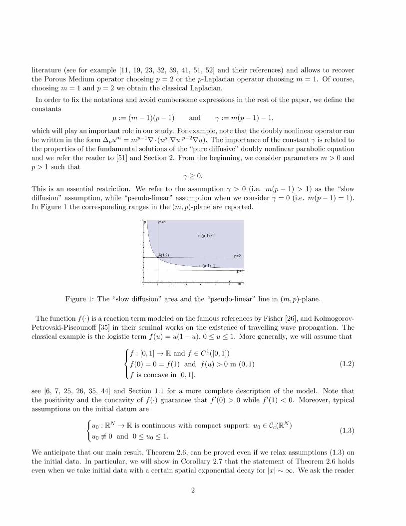
µ := (m− 1)(p− 1) and γ := m(p− 1)− 1,

which will play an important role in our study. For example, note that the doubly nonlinear operator canbe written in the form ∆pu

m = mp−1∇·(uµ|∇u|p−2∇u). The importance of the constant γ is related tothe properties of the fundamental solutions of the “pure diffusive” doubly nonlinear parabolic equationand we refer the reader to [51] and Section 2. From the beginning, we consider parameters m > 0 andp > 1 such that

γ ≥ 0.

This is an essential restriction. We refer to the assumption γ > 0 (i.e. m(p − 1) > 1) as the “slowdiffusion” assumption, while “pseudo-linear” assumption when we consider γ = 0 (i.e. m(p− 1) = 1).In Figure 1 the corresponding ranges in the (m, p)-plane are reported.

m

p

m(p-1)=1

p=2

p=1

m=1

m(p-1)>1

A(1,2)

Figure 1: The “slow diffusion” area and the “pseudo-linear” line in (m, p)-plane.

The function f(·) is a reaction term modeled on the famous references by Fisher [26], and Kolmogorov-Petrovski-Piscounoff [35] in their seminal works on the existence of travelling wave propagation. Theclassical example is the logistic term f(u) = u(1− u), 0 ≤ u ≤ 1. More generally, we will assume that

f : [0, 1]→ R and f ∈ C1([0, 1])

f(0) = 0 = f(1) and f(u) > 0 in (0, 1)

f is concave in [0, 1].

(1.2)

see [6, 7, 25, 26, 35, 44] and Section 1.1 for a more complete description of the model. Note thatthe positivity and the concavity of f(·) guarantee that f ′(0) > 0 while f ′(1) < 0. Moreover, typicalassumptions on the initial datum are

u0 : RN → R is continuous with compact support: u0 ∈ Cc(RN )

u0 6≡ 0 and 0 ≤ u0 ≤ 1.(1.3)

We anticipate that our main result, Theorem 2.6, can be proved even if we relax assumptions (1.3) onthe initial data. In particular, we will show in Corollary 2.7 that the statement of Theorem 2.6 holdseven when we take initial data with a certain spatial exponential decay for |x| ∼ ∞. We ask the reader

2

to keep in mind that the assumptions on f(·) and u0(·) combined with the Maximum Principle allowus to deduce that all solutions of problem (1.1) are trapped between the steady states u = 0 and u = 1,i.e., 0 ≤ u(x, t) ≤ 1 in RN × [0,∞).

We point out that the proof the asymptotic result follows a very detailed analysis of the existence ofadmissible travelling waves which is done in Section 3 and Section 4. Actually, we are going to extendthe well-known results on the Cauchy problem (1.1) with m = 1 and p = 2 (see Subsection 1.3) to thecase m > 0 and p > 1 (such that γ > 0), trying to stress the main differences between the linear andthe nonlinear case. In particular, it will turn out that the nonlinearity of our diffusion operator causesthe appearance of nonnegative solutions with free boundaries which are not admitted in the case m = 1and p = 2. Moreover, in Section 4, we generalize the linear theory to the ranges of parameters m > 0and p > 1 such that γ = 0, which can be seen as a limit case of the choice γ > 0. Finally, we point outthat the methods used in the PDEs part (to study the asymptotic behaviour of the solution of problem(1.1)) are original and do not rely on the proofs given for the linear case, as [6, 7, 35].

1.1 The Fisher-KPP model

The reaction term f(u) = u(1 − u) was introduced in the same year, by Fisher ([26]) in the contextof the dynamics of populations, and by Kolmogorov, Petrovsky and Piscounoff ([35]) who studied asimilar model with a more general function f(·). It was followed by a wide literature, using bothprobabilistic and analytic methods (see [6, 7, 25, 43, 44, 50]).

Let us recall the model presented in [26]. Fisher considered a density of population distributeduniformly on the real line and supposed that it was divided in two sub-densities or sub-groups ofindividuals ρ1 = ρ1(x, t) and ρ2 = ρ2(x, t) such that ρ1 + ρ2 = 1 (i.e., no other sub-groups wereadmitted). The idea was to modeling the evolution in time of the entire population when geneticmutations occurred in some individuals. So, in order to fix the ideas, it is possible to suppose that ρ1represents the part of the population with mutated genes, while ρ2 be the old generation. According tothe evolution theories, it was supposed that mutations improved the capacity of survival of individualsand generated a consequent competition between the new and the old generation. Then, a “rate”of gene-modification was introduced, i.e., a coefficient κ > 0 describing the “intensity of selection infavour of the mutant gene” ([26], p.355). In other words, κ represents the probability that the couplingof two individuals from different groups generated a mutant. Then, the author of [26] supposed thatthe individuals ρ1 sprawled on the real line with law −D∂xρ1, where D > 0. This formula representsthe typical flow of diffusive type caused by the movement of the individuals. Hence, according to theprevious observations Fisher obtained the equation

∂tρ1 = D∂xxρ1 + κρ1ρ2 in R× (0,∞).

Recalling that ρ1 + ρ2 = 1 and renaming ρ1 = u, he deduced the evolution equation of the mutatedindividuals

∂tu = D∂xxu+ κu(1− u) in R× (0,∞), (1.4)

which is the one-dimensional version of (1.1) with m = 1 and p = 2 and it explains the choice of thereaction term f(u) = u(1−u). Note that we can suppose D = κ = 1, after performing a simple variablescaling.

Equation (1.4) and its generalizations have been largely studied in the last century. The first resultswere showed in [26] and [35], where the authors understood that the group of mutants prevailed on

3

the other individuals, tending to occupy all the available space, and causing the extinction of the restof the population. A crucial mathematical result was discovered: the speed of proliferation of themutants is approximately constant for large times and the general solutions of (1.4) could be describedby introducing particular solutions called Travelling Waves (TWs).

1.2 Travelling waves

They are special solutions with remarkable applications, and there is a huge mathematical literaturedevoted to them. Let us review the main concepts and definitions.

Fix m > 0 and p ≥ 1 and assume that we are in space dimension 1 (note that when N = 1, the doublynonlinear operator has the simpler expression ∆pu

m = ∂x(|∂xum|p−2∂xum)). A TW solution of theequation

∂tu = ∆pum + f(u) in R× (0,∞) (1.5)

is a solution of the form u(x, t) = ϕ(ξ), where ξ = x+ ct, c > 0 and the profile ϕ(·) is a real function.In our application to the Fisher-KPP problem, we will need the profile to satisfy

0 ≤ ϕ ≤ 1, ϕ(−∞) = 0, ϕ(∞) = 1 and ϕ′ ≥ 0. (1.6)

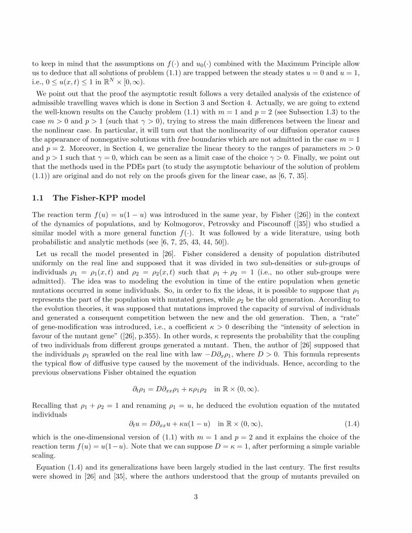
In that case say that u(x, t) = ϕ(ξ) is an admissible TW solution. Similarly, one can consider admissibleTWs of the form u(x, t) = ϕ(ξ) with ξ = x− ct, ϕ decreasing and such that ϕ(−∞) = 1 and ϕ(∞) = 0.But it is easy to see that these two options are equivalent, since the the shape of the profile of thesecond one can be obtained by reflection of the first one, ϕ−c(ξ) = ϕc(−ξ), and it moves in theopposite direction of propagation. In the rest of the paper, we will use both types of TWs, but if it isnot specified, the reader is supposed to consider TW solutions defined as in (1.6). We recall that, sinceadmissible TWs join the levels u = 0 and u = 1, they are called “change of phase type” and are reallyimportant in many physical applications.

0

1

Positive TWFinite TW

0

1

Reflected Pos. TW

Reflected Fin. TW

Figure 2: Examples of admissible TWs and their “reflections”: Finite and Positive types

Finally, an admissible TW is said finite if ϕ(ξ) = 0 for ξ ≤ ξ0 and/or ϕ(ξ) = 1 for ξ ≥ ξ1, or positive ifϕ(ξ) > 0, for all ξ ∈ R. The line x = ξ0 − ct that separates the regions of positivity and vanishing ofu(x, t) is then called the free boundary. Same name would be given to the line x = ξ1− ct and ϕ(ξ) = 1for ξ ≥ ξ1 with x1 finite, but this last situation will not happen.

4

Though the TWs are essentially one-dimensional objects, there is a natural extension to several dimen-sions. Indeed, we can consider equation (1.5) in dimension N ≥ 1 and look for solution in the formu(x, t) = ϕ(x ·n+ ct) where x ∈ RN and n is a unit vector of RN . Note that the direction of the vectorn coincides with the direction of propagation of the wave and we are taken back to the study of (1.5)in spatial dimension 1.

1.3 Results for linear diffusion

As we have said, the case of linear diffusion has been extensively studied. In [6, 7, 35] it has beenproved that the existence of admissible TWs strongly depends on the speed of propagation c > 0 of thewave and in particular, on the local behaviour of the solution near the steady states u = 0 and u = 1.In particular, they showed the following theorem, assuming the parameters D = κ = 1.

Theorem 1.1 There exists a critical speed of propagation c∗ = 2 such that for all 0 < c < c∗, thereare not admissible TW solutions for equation (1.4), while for all c ≥ c∗, there exists a unique positiveTW solution (up to its horizontal reflection or horizontal displacement).

In this case there are no free boundaries. Theorem 1.1 and suitable comparison principles allowed theauthors of [6] and [7] to understand the asymptotic behaviour of the general solution of (1.4) stated inthe following theorem.

Theorem 1.2 The solution u = u(x, t) of equation (1.4) with initial datum of type (1.3) satisfies

limt→∞

u(ξ − ct, t) =

1 if |c| < c∗

0 if |c| > c∗,

for all ξ ∈ R. Equivalently, we can reformulate the previous limit saying that

u(x, t)→ 1 uniformly in |x| ≤ ct as t→∞, for all 0 < c < c∗,

u(x, t)→ 0 uniformly in |x| ≥ ct as t→∞, for all c > c∗.

We recall that in [6] and [7], the authors worked with a more general reaction term f(·) with propertiessimilar to (1.2). It then turns out that the critical speed of propagation depends on the reaction:c∗ = 2

√f ′(0) (which evidently generalizes the case f(u) = u(1− u)). Finally, in [7], they extended the

previous theorem when the spatial dimension is greater than one.

The assertions of Theorem 1.2 mean that the steady state u = 1 is asymptotically stable while thenull solution u = 0 is unstable and, furthermore, the asymptotic stability/instability can be measuredin terms of speed of convergence of the solution which, in this case, is asymptotically linear in distanceof the front location as function of time. From the point of view of the applications, it is possible tostate that the density u(x, t) tends to saturate the space and its resources, while the rate of propagationin space is linear with constant c∗. However, it is not clear what are the properties of the solutionu = u(x, t) on the moving coordinate x = ξ − c∗t when we consider the critical speed and still it seemsto represent a very challenging problem. We will give some information in the last section for thereader’s convenience.

5

1.4 Nonlinear diffusion

Alongside the just described studies, researchers have paid attention to nonlinear variants of the Fisher-KPP model which are interesting for the applications. The mathematical issue is whether the TWparadigm to explain the long-time propagation of the solution is valid or not.

Finite propagation. The Porous Medium case. As we have just mentioned, an interesting classof such new models concerns equations with nonlinear diffusion. For instance, in [4] and [5], Aronsonconsidered a modified version of equation (1.4), introducing a nonlinear Porous Medium diffusion:

∂tu = ∂xx(um) + f(u) in R× (0,∞), (1.7)

with f(·) satisfying (1.2) and m > 1. In [5], he proved a nonlinear version of Theorem 1.1 whichasserts: for all m > 1, there exists a critical speed of propagation c∗ = c∗(m) > 0 such that there arenot admissible TW solutions for equation (1.7) for all 0 < c < c∗(m), whilst for all c ≥ c∗(m) thereexists exactly one admissible TW solution. Moreover, the TW corresponding to the speed c∗(m) isfinite, while for c > c∗(m) the TWs are positive.

Hence, it is clear that the nonlinear diffusion presents an interesting peculiarity: the TW correspondingto the value c∗(m) is finite, which means that free boundaries appear exactly as in the simpler PorousMedium equation (see for instance [51] and [52]). This observation suggests that the general solution ofequation (1.7) with initial datum (1.3) has a free boundary too and this is evidently a really interestingdifference respect to the linear case. Similar results were showed in a series of papers ([16, 17, 18])for equation (1.7) with a non-smooth reaction term f(u) = aun(1 − u) where a > 0 and n ∈ R. Theauthors’ concern was to study the the combination of a slow diffusion term given by ∂xxu

m (m > 1)and strong reaction term given by the singularity in the origin of the function un when n < 1. Theyproved the following theorem (see Theorem 7.1 of [17]).

Theorem 1.3 Let m > 1, n ∈ R and q := m + n − 2 and a = 1/m. Then there exist admissible TWsolutions for equation (1.7) with f(u) = aun(1− n) if and only if q ≥ 0.

Moreover, for all q ≥ 0, there exists a critical speed c∗ = c∗(q) > 0 such that equation (1.7) withf(u) = aun(1 − n) possesses a unique admissible TW for all c ≥ c∗(q) and does not have admissibleTWs for 0 < c < c∗(q).

Finally, the TW corresponding to the speed c∗(q) is finite while the TWs with c > c∗(q) are finite ifand only if 0 < n < 1.

Theorem 1.3 is really interesting since it gives the quantitative “combination” between slow diffusionand strong reaction in order to have only finite TWs. We will sketch the proof of a generalization ofthis result at the end of the paper (see Section 10).

The p -Laplacian case. Recently, the authors of [22] and [27] studied the existence of admissibleTW solution for the p-Laplacian reaction-diffusion equation

∂tu = ∂x(|∂xu|p−2∂xu) + f(u) in R× (0,∞), (1.8)

for p > 1. They considered a quite general reaction term f(·) satisfyingf(0) = 0 = f(1) and f(u) > 0 in (0, 1)

supu∈(0,1) u1−p′f(u) = Mp < +∞

6

where p′ is the conjugated of p, i.e., 1/p+1/p′ = 1. They proved (see Proposition 2 of [22]) the existenceof a critical speed of propagation c∗ > 0 depending only on p and f(·) such that equation (1.8) possessesadmissible TW solutions if and only if c ≥ c∗ and, furthermore, they obtained the interesting boundc∗ ≤ p1/p(p′Mp)

1/p′ . Moreover, with the additional assumption

limu→0+

u1−p′f(u) = sup

u∈(0,1)u1−p

′f(u) = Mp < +∞

they proved that c∗ = p1/p(p′Mp)1/p′ . Finally, they focused on the study of TWs for equation (1.8) for

different kinds of reaction terms (see [22] and [27] for a complete treatise).

The scene is set for us to investigate what happens in the presence of a doubly nonlinear diffusion.However, we have to underline we are not only interested in studying the existence of admissible speedsof propagation, but also in understanding the properties of the admissible TWs, i.e., if they are finitewith free boundary or everywhere positive. Finally, our main goal is to apply the ODEs results to thestudy of the long-time behaviour of the PDEs problem (1.1).

2 Doubly nonlinear diffusion. Preliminaries and main results

Now we present some basic results concerning the Barenblatt solutions of the “pure diffusive” doublynonlinear parabolic equation which are essential to develop our study in the next sections (the referencefor this issue is [51]). Moreover, we recall some basic facts on existence, uniqueness, regularity andMaximum Principles for the solutions of problem (1.1).

Barenblatt solutions. Fix m > 0 and p > 1 such that γ ≥ 0 and consider the “pure diffusive”doubly nonlinear problem:

∂tu = ∆pum in RN × (0,∞)

u(t)→Mδ0 in RN as t→ 0,(2.1)

where Mδ0(·) is the Dirac’s function with mass M > 0 in the origin of RN and the convergence has tobe intended in the sense of measures.

Case γ > 0. It has been proved (see [51]) that problem (2.1) admits continuous weak solutions inself-similar form BM (x, t) = t−αFM (xt−α/N ), called Barenblatt solutions, where the profile FM (·) isdefined by the formula:

FM (ξ) =(CM − k|ξ|

pp−1

) p−1γ

+

where

α =1

γ + p/N, k =

γ

p

( αN

) 1p−1

and CM > 0 is determined in terms of the mass choosing M =∫RN BM (x, t)dx (see [51] for a complete

treatise). It will be useful to keep in mind that we have the formula

BM (x, t) = MB1(x,Mγt) (2.2)

which describes the relationship between the Barenblatt solution of mass M > 0 and mass M = 1. Weremind the reader that the solution has a free boundary which separates the set in which the solutionis positive from the set in which it is identically zero (“slow” diffusion case).

7

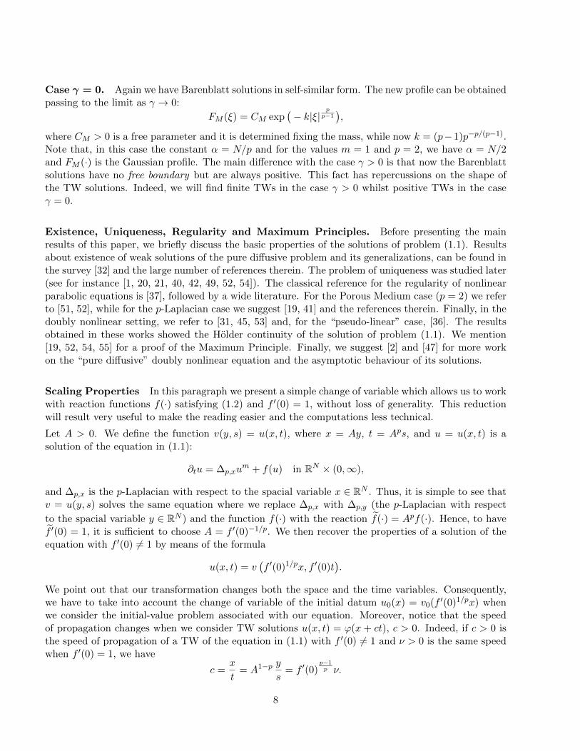
Case γ = 0. Again we have Barenblatt solutions in self-similar form. The new profile can be obtainedpassing to the limit as γ → 0:

FM (ξ) = CM exp(− k|ξ|

pp−1),

where CM > 0 is a free parameter and it is determined fixing the mass, while now k = (p−1)p−p/(p−1).Note that, in this case the constant α = N/p and for the values m = 1 and p = 2, we have α = N/2and FM (·) is the Gaussian profile. The main difference with the case γ > 0 is that now the Barenblattsolutions have no free boundary but are always positive. This fact has repercussions on the shape ofthe TW solutions. Indeed, we will find finite TWs in the case γ > 0 whilst positive TWs in the caseγ = 0.

Existence, Uniqueness, Regularity and Maximum Principles. Before presenting the mainresults of this paper, we briefly discuss the basic properties of the solutions of problem (1.1). Resultsabout existence of weak solutions of the pure diffusive problem and its generalizations, can be found inthe survey [32] and the large number of references therein. The problem of uniqueness was studied later(see for instance [1, 20, 21, 40, 42, 49, 52, 54]). The classical reference for the regularity of nonlinearparabolic equations is [37], followed by a wide literature. For the Porous Medium case (p = 2) we referto [51, 52], while for the p-Laplacian case we suggest [19, 41] and the references therein. Finally, in thedoubly nonlinear setting, we refer to [31, 45, 53] and, for the “pseudo-linear” case, [36]. The resultsobtained in these works showed the Holder continuity of the solution of problem (1.1). We mention[19, 52, 54, 55] for a proof of the Maximum Principle. Finally, we suggest [2] and [47] for more workon the “pure diffusive” doubly nonlinear equation and the asymptotic behaviour of its solutions.

Scaling Properties In this paragraph we present a simple change of variable which allows us to workwith reaction functions f(·) satisfying (1.2) and f ′(0) = 1, without loss of generality. This reductionwill result very useful to make the reading easier and the computations less technical.

Let A > 0. We define the function v(y, s) = u(x, t), where x = Ay, t = Aps, and u = u(x, t) is asolution of the equation in (1.1):

∂tu = ∆p,xum + f(u) in RN × (0,∞),

and ∆p,x is the p-Laplacian with respect to the spacial variable x ∈ RN . Thus, it is simple to see thatv = u(y, s) solves the same equation where we replace ∆p,x with ∆p,y (the p-Laplacian with respect

to the spacial variable y ∈ RN ) and the function f(·) with the reaction f(·) = Apf(·). Hence, to havef ′(0) = 1, it is sufficient to choose A = f ′(0)−1/p. We then recover the properties of a solution of theequation with f ′(0) 6= 1 by means of the formula

u(x, t) = v(f ′(0)1/px, f ′(0)t

).

We point out that our transformation changes both the space and the time variables. Consequently,we have to take into account the change of variable of the initial datum u0(x) = v0(f

′(0)1/px) whenwe consider the initial-value problem associated with our equation. Moreover, notice that the speedof propagation changes when we consider TW solutions u(x, t) = ϕ(x + ct), c > 0. Indeed, if c > 0 isthe speed of propagation of a TW of the equation in (1.1) with f ′(0) 6= 1 and ν > 0 is the same speedwhen f ′(0) = 1, we have

c =x

t= A1−p y

s= f ′(0)

p−1p ν.

8

This last formula will be useful since it clearly shows how the propagation speed changes when wechange the derivative f ′(0). Thus, from now on, we will try to make explicit the dependence of thepropagation speeds on the quantity f ′(0) by using the previous formula. This fact allows us to stateour results in general terms and, at the same time, in a standard and clear way.

2.1 Main results and organization of the paper

The paper is divided in two main parts: the first one, is the ODE analysis of the existence of TWsolutions joining the critical levels u = 0 and u = 1. These special solutions are then used in the secondpart to describe the asymptotic behaviour of general solutions of the PDE problem. Each of these twoparts is divided into sections as follows:

In Section 3 we prove an extension of Theorem 1.1, for the reaction-diffusion problem (1.1) in the casem > 0 and p > 1 such that γ > 0. We study the equation

∂tu = ∂x(|∂xum|p−2∂xum) + f(u) in R× (0,∞). (2.3)

and show the following result. Let’s recall that γ = m(p− 1)− 1.

Theorem 2.1 Let m > 0 and p > 1 such that γ > 0. Then there exists a unique c∗ = c∗(m, p) > 0such that equation (2.3) possesses a unique admissible TW for all c ≥ c∗(m, p) and does not haveadmissible TWs for 0 < c < c∗(m, p). Uniqueness is understood as before, up to reflection or horizontaldisplacement.

Moreover, the TW corresponding to the value c = c∗(m, p) is finite (i.e., it vanishes in an infinitehalf-line), while the TWs corresponding to the values c > c∗(m, p) are positive everywhere.

When we say unique we are in fact referring to the TWs with increasing profile, a second equivalentsolution is obtained by reflection. Furthermore, even though there are no admissible TWs for valuesc < c∗, we construct solutions which are “partially admissible” and they will be used as sub-solutionsin the PDE analysis of the last sections.

The study of TW solutions for equation (2.3) leads us to a second order ODEs problem (see equation(3.2)). The main difference respect to the linear case is that we use a nonstandard change of variablesto pass from the second order ODE to a system of two first order ODEs (see formulas (3.4)). Moreover,we deduce the existence of the critical speed of propagation c∗(m, p) via qualitative methods while, inthe linear case (see [5] and [35]), the critical value of the parameter c > 0 was found by linearizing theODE system around its critical points.

In Section 4 we study the limit case γ = 0, that we call “pseudo-linear” (since the homogeneity of thedoubly nonlinear operator is one) and we prove the following theorem.

Theorem 2.2 Let m > 0 and p > 1 such that γ = 0. Then there exists a unique critical speed

c0∗(m, p) = p(m2f ′(0))1mp (2.4)

such that equation (2.3) possesses a unique admissible TW for all c ≥ c0∗(m, p) while it does not possessadmissible TWs for 0 < c < c0∗(m, p). All the admissible TWs are positive everywhere. Uniqueness isunderstood as in the previous theorem.

9

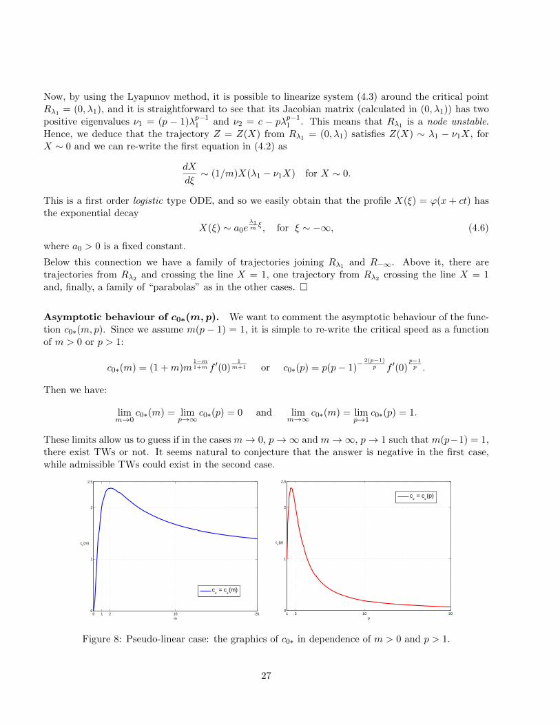
This case presents both differences and similarities respect to the case γ > 0 but we will follow theprocedure used to show Theorem 2.1 (with corresponding modifications). We ask the reader to notethat the case γ = 0 covers and generalizes the linear case m = 1 and p = 2 and to observe that themost important difference between the case γ > 0 is that there are not finite TWs, i.e., when γ = 0there are not admissible TWs with free boundary. This turns out to be a really interesting fact, sinceit means that the positivity of the admissible TWs is not due to the linearity of the diffusion operatorbut depends on the homogeneity of the operator, i.e., the relations between the diffusive parameters.To conclude the differences between the cases γ > 0 and γ = 0, we will see that the the decay to zeroof the TW with speed c ≥ c∗(m, p) (when γ = 0) differs from the decay of the positive TWs in the caseγ > 0. On the other hand, note that formula (2.4) for c0∗(m, p) agrees with the scaling for the criticalspeed in the case γ > 0:

c∗(m, p) = f ′(0)p−1p ν∗(m, p),

where ν∗(m, p) is the critical speed when γ > 0 and f ′(0) = 1. This uses the fact that the critical speedwhen γ = 0 and f ′(0) = 1 is ν0∗ = pm2/(mp), and (p− 1)→ 1/m as γ → 0.

Finally, we prove that the critical speed c∗(m, p) (when γ > 0), found in Theorem 2.1, converges tothe critical speed c0∗(m, p) (when γ = 0), found in Theorem 2.2, as γ → 0. In particular, we prove thefollowing theorem.

Theorem 2.3 Consider the region H = (m, p) : γ = m(p− 1)− 1 > 0. Then the function

(m, p) →

c∗(m, p) if γ > 0

c0∗(m, p) if γ = 0(2.5)

where c∗(m, p) is the critical speed for the values γ > 0 (found in Theorem 2.1) while c0∗(m, p) is thecritical speed for the values γ = 0 (found in Theorem 2.2), is continuous on the closure of H, i.e.,H = (m, p) : γ = m(p− 1)− 1 ≥ 0.

The previous theorem is proved in two steps. We show the continuity of the function (2.5) in the regionH in Lemma 3.1 and Corollary 3.2. Then we extend the continuity to the closure H in Lemma 4.1.

We conclude this paragraph pointing out that we will use the separate notations c∗(m, p) and c0∗(m, p)for the cases γ > 0 and γ = 0 in Section 3, Section 4, and in the statement and the proof of Corollary2.7 while, later, we will unify them writing simply c∗ or c∗(m, p) for all (m, p) ∈ H, thanks to the resultstated in Theorem 2.3.

In Section 5 we begin with the PDE analysis which is the main goal of this paper. As a first step, westudy the Cauchy problem (1.1) with a particular choice of the initial datum

u0(x) :=

ε if |x| ≤ %00 if |x| > %0.

(2.6)

where ε and %0 are positive real numbers. The solutions of problem (1.1), (2.6) are really useful sincecan be used as sub-solutions for the general problem (1.1), (1.3) (see Lemma 7.1).

We first prove a technical lemma (see Lemma 5.2) which turns out to be essential in the study of theasymptotic behaviour of the solution of problem (1.1). The main consequence of Lemma 5.2 is thefollowing proposition.

10

Proposition 2.4 Let m > 0 and p > 1 such that γ > 0 and let N ≥ 1. Then, for all %0 > 0 and forall %1 ≥ %0, there exists ε > 0 and t0 > 0, such that the solution u(x, t) of problem (1.1) with initialdatum (2.6) satisfies

u(x, t) ≥ ε in |x| ≤ %1/2 for all t ≥ t0.

This proposition asserts that for all initial datum small enough, the solution of problem (1.1) is strictlygreater than a fixed positive constant on every compact set of RN for large times. This property willresult essential for the asymptotic study of general solutions in Section 7 (see Lemma 7.1).

In Section 6 we proceed with the PDE study done in the previous section taking γ = 0 (“pseudo-linearcase”). In this case, we choose the initial datum

u0(x) :=

ε if |x| ≤ %0

a0e−b0|x|

pp−1

if |x| > %0,a0 := εeb0%

pp−10 (2.7)

where again ε, %0 and b0 are positive numbers. The different choice of the datum is due to the differentshape of the profile of the Barenblatt solutions in the case γ = 0 (see Section 2). In particular, the newdatum has not compact support, but “exponential” tails.

Basically, we repeat the procedure followed in Section 5, but, as we will see in the proof of Lemma 6.2,the are several technical differences respect to the case γ > 0. We prove the following proposition.

Proposition 2.5 Let m > 0 and p > 1 such that γ = 0 and let N ≥ 1. Then, for all %0 > 0 and forall %1 ≥ %0, there exists ε > 0 and t0 > 0, such that the solution u(x, t) of problem (1.1) with initialdatum (2.7) satisfies

u(x, t) ≥ ε in |x| ≤ %1 for all t ≥ t0.

Even though Proposition 2.5 is a version of Proposition 2.4 when γ = 0, we decided to separatetheir proofs since there are significant deviances in the techniques followed to show them. The mostimportant one respect to the case γ > 0 is that we work with positive Barenblatt solutions and the freeboundaries, which constitute the most technical “trouble”, are not present.

In Section 7, 8, and 9 we address to the problem of the asymptotic behaviour of the solution ofproblem (1.1) for large times and we prove the following theorem.

Theorem 2.6 Let m > 0 and p > 1 such that γ ≥ 0, and let N ≥ 1.

(i) For all 0 < c < c∗(m, p), the solution u(x, t) of the initial-value problem (1.1) with initial datum(1.3) satisfies

u(x, t)→ 1 uniformly in |x| ≤ ct as t→∞.

(ii) Moreover, for all c > c∗(m, p) it satisfies,

u(x, t)→ 0 uniformly in |x| ≥ ct as t→∞.

This result extends Theorem 1.2 to the all range of parameters m > 0 and p > 1 such that γ ≥ 0and it states that the part of the population with mutant gene invades all the available space withspeed of propagation c∗(m, p), driving to extinction the rest of the individuals. In the case γ > 0,

11

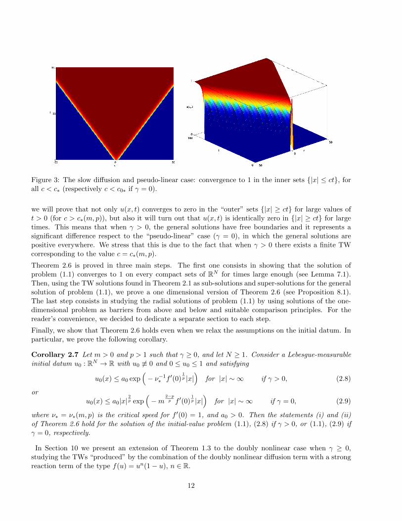
Figure 3: The slow diffusion and pseudo-linear case: convergence to 1 in the inner sets |x| ≤ ct, forall c < c∗ (respectively c < c0∗ if γ = 0).

we will prove that not only u(x, t) converges to zero in the “outer” sets |x| ≥ ct for large values oft > 0 (for c > c∗(m, p)), but also it will turn out that u(x, t) is identically zero in |x| ≥ ct for largetimes. This means that when γ > 0, the general solutions have free boundaries and it represents asignificant difference respect to the “pseudo-linear” case (γ = 0), in which the general solutions arepositive everywhere. We stress that this is due to the fact that when γ > 0 there exists a finite TWcorresponding to the value c = c∗(m, p).

Theorem 2.6 is proved in three main steps. The first one consists in showing that the solution ofproblem (1.1) converges to 1 on every compact sets of RN for times large enough (see Lemma 7.1).Then, using the TW solutions found in Theorem 2.1 as sub-solutions and super-solutions for the generalsolution of problem (1.1), we prove a one dimensional version of Theorem 2.6 (see Proposition 8.1).The last step consists in studying the radial solutions of problem (1.1) by using solutions of the one-dimensional problem as barriers from above and below and suitable comparison principles. For thereader’s convenience, we decided to dedicate a separate section to each step.

Finally, we show that Theorem 2.6 holds even when we relax the assumptions on the initial datum. Inparticular, we prove the following corollary.

Corollary 2.7 Let m > 0 and p > 1 such that γ ≥ 0, and let N ≥ 1. Consider a Lebesgue-measurableinitial datum u0 : RN → R with u0 6≡ 0 and 0 ≤ u0 ≤ 1 and satisfying

u0(x) ≤ a0 exp(− ν−1∗ f ′(0)

1p |x|

)for |x| ∼ ∞ if γ > 0, (2.8)

oru0(x) ≤ a0|x|

2p exp

(−m

2−pp f ′(0)

1p |x|

)for |x| ∼ ∞ if γ = 0, (2.9)

where ν∗ = ν∗(m, p) is the critical speed for f ′(0) = 1, and a0 > 0. Then the statements (i) and (ii)of Theorem 2.6 hold for the solution of the initial-value problem (1.1), (2.8) if γ > 0, or (1.1), (2.9) ifγ = 0, respectively.

In Section 10 we present an extension of Theorem 1.3 to the doubly nonlinear case when γ ≥ 0,studying the TWs “produced” by the combination of the doubly nonlinear diffusion term with a strongreaction term of the type f(u) = un(1− u), n ∈ R.

12

In Section 11 we give a detailed proof of formula (4.5) which describes the asymptotic behaviour ofthe TW solution with critical speed of propagation when γ = 0, and is linked to the choice of the initialdatum (2.9).

In Section 12 we conclude the paper by discussing some issues related to our study. Firstly, as wehave anticipated earlier, we briefly report the results obtained in [8, 9] and [29] on the behaviour of thegeneral solutions of problem (1.4) on the moving coordinate ξ = x− c∗t. Then we present some resultsand open problems concerning the F-KPP theory when we deal with a “fast diffusion” term. Finally,we comment briefly what our results tell about the limit cases m = 0, p =∞ and m =∞, p = 1 withthe condition m(p− 1) = 1 (γ = 0).

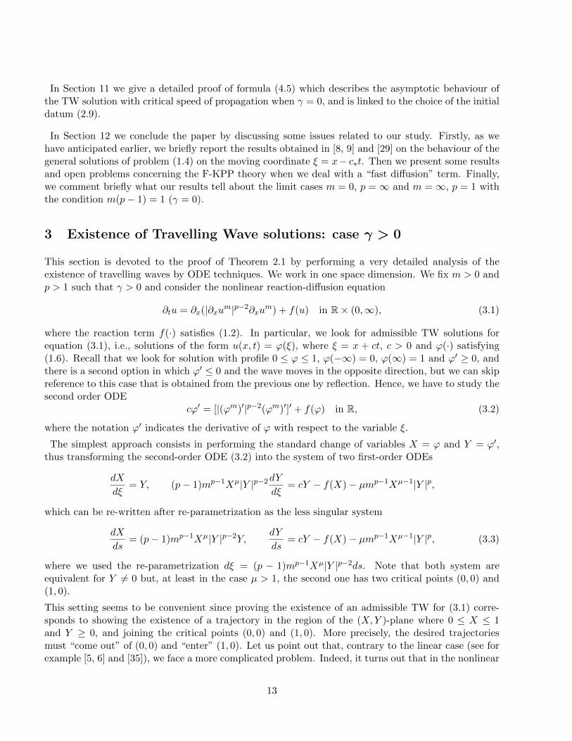
3 Existence of Travelling Wave solutions: case γ > 0

This section is devoted to the proof of Theorem 2.1 by performing a very detailed analysis of theexistence of travelling waves by ODE techniques. We work in one space dimension. We fix m > 0 andp > 1 such that γ > 0 and consider the nonlinear reaction-diffusion equation

∂tu = ∂x(|∂xum|p−2∂xum) + f(u) in R× (0,∞), (3.1)

where the reaction term f(·) satisfies (1.2). In particular, we look for admissible TW solutions forequation (3.1), i.e., solutions of the form u(x, t) = ϕ(ξ), where ξ = x + ct, c > 0 and ϕ(·) satisfying(1.6). Recall that we look for solution with profile 0 ≤ ϕ ≤ 1, ϕ(−∞) = 0, ϕ(∞) = 1 and ϕ′ ≥ 0, andthere is a second option in which ϕ′ ≤ 0 and the wave moves in the opposite direction, but we can skipreference to this case that is obtained from the previous one by reflection. Hence, we have to study thesecond order ODE

cϕ′ = [|(ϕm)′|p−2(ϕm)′]′ + f(ϕ) in R, (3.2)

where the notation ϕ′ indicates the derivative of ϕ with respect to the variable ξ.

The simplest approach consists in performing the standard change of variables X = ϕ and Y = ϕ′,thus transforming the second-order ODE (3.2) into the system of two first-order ODEs

dX

dξ= Y, (p− 1)mp−1Xµ|Y |p−2dY

dξ= cY − f(X)− µmp−1Xµ−1|Y |p,

which can be re-written after re-parametrization as the less singular system

dX

ds= (p− 1)mp−1Xµ|Y |p−2Y, dY

ds= cY − f(X)− µmp−1Xµ−1|Y |p, (3.3)

where we used the re-parametrization dξ = (p − 1)mp−1Xµ|Y |p−2ds. Note that both system areequivalent for Y 6= 0 but, at least in the case µ > 1, the second one has two critical points (0, 0) and(1, 0).

This setting seems to be convenient since proving the existence of an admissible TW for (3.1) corre-sponds to showing the existence of a trajectory in the region of the (X,Y )-plane where 0 ≤ X ≤ 1and Y ≥ 0, and joining the critical points (0, 0) and (1, 0). More precisely, the desired trajectoriesmust “come out” of (0, 0) and “enter” (1, 0). Let us point out that, contrary to the linear case (see forexample [5, 6] and [35]), we face a more complicated problem. Indeed, it turns out that in the nonlinear

13

diffusion case, the Lyapunov linearization method ([15], Chapter 8) used to analyze the local behaviourof the trajectories near the critical points cannot be applied since system (3.3) is heavily nonlinear.

System (3.3) admits a large collection of trajectories and corresponding TWs. Hence, the very problemis to understand how to discern between different types of trajectories “coming out” of the steady state(0, 0). The flow around this point has a complicated structure, so, following the methods inspired inthe study of the Porous Medium case (see [17]), we introduce the new variables

X = ϕ and Z =

(m(p− 1)

γϕ

γp−1

)′= mX

µ−1p−1X ′, (3.4)

using the fact that γ = µ+ p− 2. These variables correspond to the density and the derivative of thepressure profile (see [23]). Assuming only X ≥ 0, we obtain the first-order ODE system

dX

dξ= (1/m)X

1−µp−1Z, m(p− 1)X

γp−1 |Z|p−2 dZ

dξ= cZ − |Z|p −mX

µ−1p−1 f(X), (3.5)

that again can be re-written as the non-singular system

dX

dτ= (p− 1)X|Z|p−2Z, dZ

dτ= cZ − |Z|p −mX

µ−1p−1 f(X) (3.6)

where we use the new re-parametrization dξ = m(p−1)Xγp−1 |Z|p−2dτ . Note that, since 0 < γ = µ+p−2,

the functionfm,p(X) = mX

µ−1p−1 f(X) = mX

γp−1−1f(X)

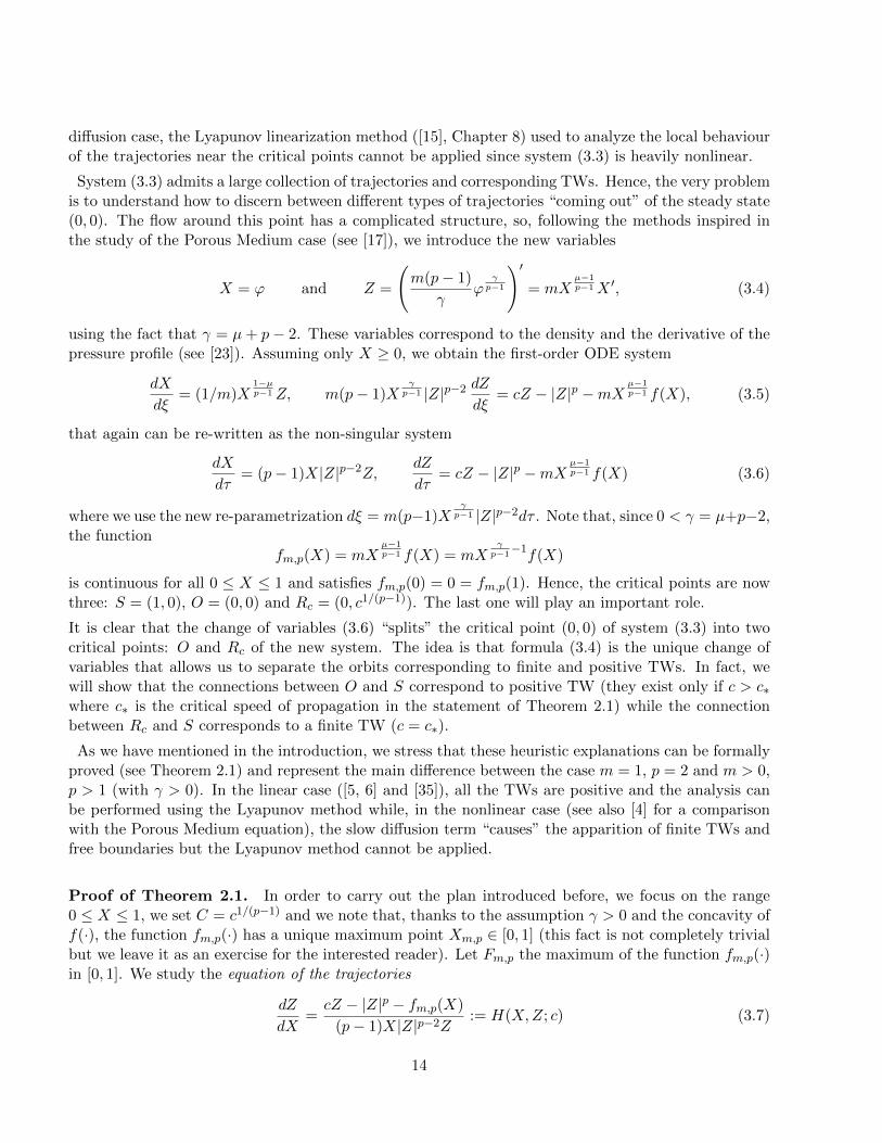
is continuous for all 0 ≤ X ≤ 1 and satisfies fm,p(0) = 0 = fm,p(1). Hence, the critical points are nowthree: S = (1, 0), O = (0, 0) and Rc = (0, c1/(p−1)). The last one will play an important role.

It is clear that the change of variables (3.6) “splits” the critical point (0, 0) of system (3.3) into twocritical points: O and Rc of the new system. The idea is that formula (3.4) is the unique change ofvariables that allows us to separate the orbits corresponding to finite and positive TWs. In fact, wewill show that the connections between O and S correspond to positive TW (they exist only if c > c∗where c∗ is the critical speed of propagation in the statement of Theorem 2.1) while the connectionbetween Rc and S corresponds to a finite TW (c = c∗).

As we have mentioned in the introduction, we stress that these heuristic explanations can be formallyproved (see Theorem 2.1) and represent the main difference between the case m = 1, p = 2 and m > 0,p > 1 (with γ > 0). In the linear case ([5, 6] and [35]), all the TWs are positive and the analysis canbe performed using the Lyapunov method while, in the nonlinear case (see also [4] for a comparisonwith the Porous Medium equation), the slow diffusion term “causes” the apparition of finite TWs andfree boundaries but the Lyapunov method cannot be applied.

Proof of Theorem 2.1. In order to carry out the plan introduced before, we focus on the range0 ≤ X ≤ 1, we set C = c1/(p−1) and we note that, thanks to the assumption γ > 0 and the concavity off(·), the function fm,p(·) has a unique maximum point Xm,p ∈ [0, 1] (this fact is not completely trivialbut we leave it as an exercise for the interested reader). Let Fm,p the maximum of the function fm,p(·)in [0, 1]. We study the equation of the trajectories

dZ

dX=cZ − |Z|p − fm,p(X)

(p− 1)X|Z|p−2Z:= H(X,Z; c) (3.7)

14

after eliminating the parameter τ , and look for solutions defined for 0 ≤ X ≤ 1 and linking the criticalpoints Rc and S for some c > 0. The main difference with respect to the Porous Medium and the linearcase (see [6] and [17]) is that the critical points are all degenerate and it is impossible to describe thelocal behaviour of the trajectories by linearizing the system (3.6) around S. In what follows, we studysome local and global properties of the equation (3.7) with other qualitative ODE methods in order toobtain a clear view of the graph of the trajectories.

Step1. Firstly, we study the null isoclines of system (3.6), i.e., the set of the points (X,Z) with0 ≤ X ≤ 1 and Z ≥ 0 such that H(X,Z; c) = 0. Hence, we have to solve the equation

cZ − Zp = fm,p(X) in [0, 1]× [0,∞). (3.8)

Defining

c0 = c0(m, p) := p

(Fm,pp− 1

)(p−1)/p

,

it is simple to see that for c < c0 the graph of the isoclines is composed by two branches joining thepoint O with Rc and the point (1, 0) with (1, C), while for c > c0 the branches link the point O with Sand the point Rc with (1, C). As c approaches the value c0 the branches move nearer and they touchin the point (Xm,p, (c0/p)

1/(p−1)) for c = c0. Note that the value c0(m, p) is critical in the study of theisoclines and it is found by imposing

maxZ∈[0,C]

cZ − Zp = Fm,p. (3.9)

0 10

0.5

1

X

Z

0 10

0.5

1

X

Z

Figure 4: Null isoclines of system (3.6): Case c < c0 and c > c0.

For c < c0, the trajectories in the region between the two branches have negative slopes, while thosein the region between the Z-axis and the left branch and between the right branch and the line X = 1have positive slopes. Conversely, for c > c0 the trajectories in the region between the two branches havepositive slopes while, those in the region between the bottom-branch and the X-axis and between theline Z = C and the top-branch have negative slopes. Finally, for c = c0, it is simple to see that in theregions between the bottom-branch and the X-axis and between the line Z = C and the top-branch thetrajectories have negative slopes and they have positive slopes in the rest of the rectangle [0, 1]× [0, C].We conclude this paragraph noting that for all c > 0 the trajectories have negative slopes for Z > Cand positive slopes for Z < 0.

Step2. We prove the existence and the uniqueness of solutions of (3.7) “entering” in the point S.

15

Case p = 2. If p = 2, it is not difficult to linearize system (3.6) through Lyapunov method and showingthat the point S is a saddle. Moreover, it follows that there exists exactly one locally linear trajectoryin the region [0, 1]× [0,∞) “entering” in S with slope λS = (c−

√c2 − 4mf ′(1))/2.

Case p > 2. Substituting the expression Z = λ(1−X), λ > 0 in the equation of trajectories (3.7) andtaking X ∼ 1 we get

−λ = H(X,λ(1−X)) ∼ cλ(1−X) +mf ′(1)(1−X)

(p− 1)λ(p−1)(1−X)p−1, for X ∼ 1

which can be rewritten as

−(p− 1)λp(1−X)p−2 ∼ cλ+mf ′(1), for X ∼ 1.

Since the left side goes to zero as X → 1, the previous relation is satisfied only if λ = −mc−1f ′(1) :=λ+S > 0 (note that this coefficient coincides with the slope of the null isocline near X = 1). Hence, forp > 2, there exists at least one trajectory Tc which “enters” into the point S and it is linear near thiscritical point. Note that the approximation Z(X) ∼ λ+S (1 −X) as X ∼ 1 can be improved with highorder terms. However, we are basically interested in proving the existence of a trajectory “entering” inS and we avoid to present technical computations which can be performed by the interested reader.

To prove the uniqueness of the “entering orbit”, we begin by showing that the trajectory Tc (whichsatisfies Z(X) ∼ λ+S (1−X) as X ∼ 1) is “repulsive” near X = 1. It is sufficient to prove that the partialderivative of the function H with respect to the variable Z is strictly positive when it is calculated onthe trajectory Tc and X ∼ 1. It is straightforward to see that

∂H

∂Z(X,λ+S (1−X)) ∼ m

D(X)[−cλ+S (p− 2)(1−X)− (p− 1)f ′(1)(1−X)]

∼ −mf′(1)

D(X) 0, for X ∼ 1

where D(X) = (p − 1)(λ+S )p(1 − X)p−1. Hence, our trajectory is “repulsive” near the point S, i.e.,there are not other locally linear trajectories which “enter” into the point S with slope λ+S .

Now, we claim that Tc is the unique trajectory “entering” into the point S. Indeed, recalling the factthat Tc has the same slope of the null isoclines near S and using the fact that ∂H/∂Z > 0 along Tcfor X ∼ 1, it is evident that trajectories from S above Tc are not admitted. Furthermore, a simplecalculation shows that for all 0 < X < 1 fixed and Z positive but small, the second derivative isnegative:

d2Z

dX2∼ − fm,p(X)

(p− 1)X2Z2(p−1)

(c

p− 1+fm,p(X)

Z

)< 0, for Z ∼ 0+.

Hence, we deduce our assertion observing that all trajectories “entering” into S and lying below Tchave to be convex, which is a contradiction with the previous formula.

Case 1 < p < 2. Proceeding as before, it is not difficult to prove that when 1 < p < 2, thereexists a trajectory “entering” in S with local behaviour Z ∼ λ−S (1 − X)2/p for X ∼ 1 and λ−S :=−pmf ′(1)/[2(p − 1)]1/p. Note that in this case the trajectory is not locally linear but presents apower-like local behaviour around S with power greater than one. Moreover, exactly as in the casep > 2, it is simple to see that this trajectory is “repulsive”. It remains to prove that our trajectory isthe unique “entering” in S. Note that the computation of the second derivative is still valid. Moreover,

16

in order to show that there are no orbits between our trajectory and the branch of the null isoclines,we consider the two-parameters family of curves:

Za(x) = λ−S (1−X)a, 1 < a < 2/p

and we use an argument with invariant regions. We compute the derivative

dZa/dX

dZ/dX(X,Za(X); c) =

dZa/dX(X)

H(X,Za(X); c)∼−a(p− 1)(λ−S )p

mf ′(1)(1−X)ap−2 ∼ +∞ as X ∼ 1

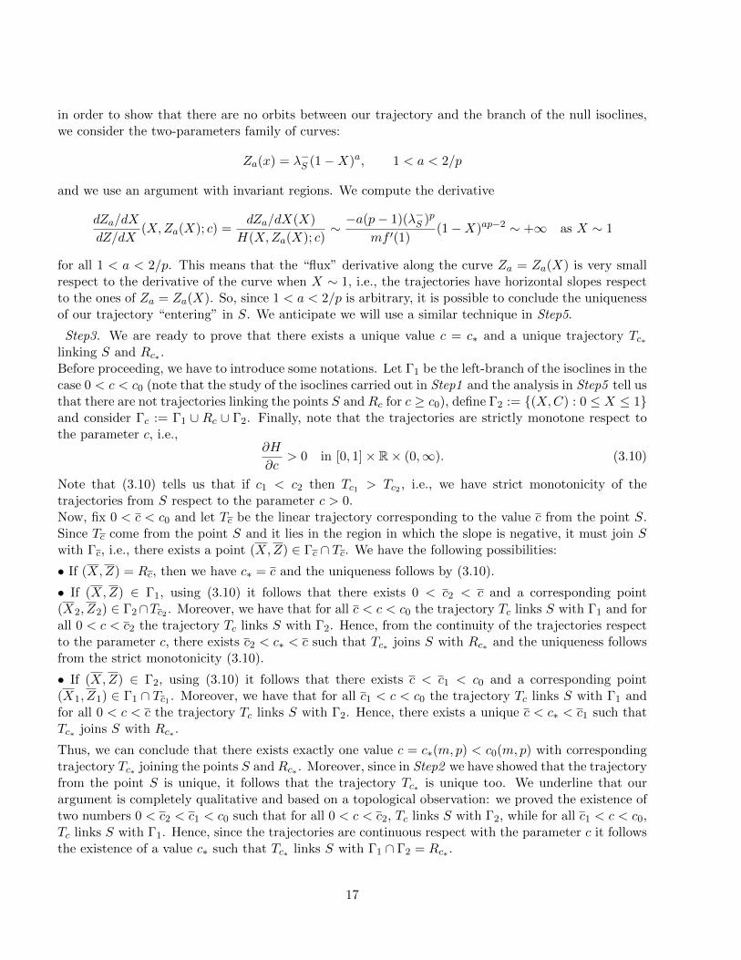
for all 1 < a < 2/p. This means that the “flux” derivative along the curve Za = Za(X) is very smallrespect to the derivative of the curve when X ∼ 1, i.e., the trajectories have horizontal slopes respectto the ones of Za = Za(X). So, since 1 < a < 2/p is arbitrary, it is possible to conclude the uniquenessof our trajectory “entering” in S. We anticipate we will use a similar technique in Step5.

Step3. We are ready to prove that there exists a unique value c = c∗ and a unique trajectory Tc∗linking S and Rc∗ .Before proceeding, we have to introduce some notations. Let Γ1 be the left-branch of the isoclines in thecase 0 < c < c0 (note that the study of the isoclines carried out in Step1 and the analysis in Step5 tell usthat there are not trajectories linking the points S and Rc for c ≥ c0), define Γ2 := (X,C) : 0 ≤ X ≤ 1and consider Γc := Γ1 ∪ Rc ∪ Γ2. Finally, note that the trajectories are strictly monotone respect tothe parameter c, i.e.,

∂H

∂c> 0 in [0, 1]× R× (0,∞). (3.10)

Note that (3.10) tells us that if c1 < c2 then Tc1 > Tc2 , i.e., we have strict monotonicity of thetrajectories from S respect to the parameter c > 0.Now, fix 0 < c < c0 and let Tc be the linear trajectory corresponding to the value c from the point S.Since Tc come from the point S and it lies in the region in which the slope is negative, it must join Swith Γc, i.e., there exists a point (X,Z) ∈ Γc ∩ Tc. We have the following possibilities:

• If (X,Z) = Rc, then we have c∗ = c and the uniqueness follows by (3.10).

• If (X,Z) ∈ Γ1, using (3.10) it follows that there exists 0 < c2 < c and a corresponding point(X2, Z2) ∈ Γ2∩Tc2 . Moreover, we have that for all c < c < c0 the trajectory Tc links S with Γ1 and forall 0 < c < c2 the trajectory Tc links S with Γ2. Hence, from the continuity of the trajectories respectto the parameter c, there exists c2 < c∗ < c such that Tc∗ joins S with Rc∗ and the uniqueness followsfrom the strict monotonicity (3.10).

• If (X,Z) ∈ Γ2, using (3.10) it follows that there exists c < c1 < c0 and a corresponding point(X1, Z1) ∈ Γ1 ∩ Tc1 . Moreover, we have that for all c1 < c < c0 the trajectory Tc links S with Γ1 andfor all 0 < c < c the trajectory Tc links S with Γ2. Hence, there exists a unique c < c∗ < c1 such thatTc∗ joins S with Rc∗ .

Thus, we can conclude that there exists exactly one value c = c∗(m, p) < c0(m, p) with correspondingtrajectory Tc∗ joining the points S and Rc∗ . Moreover, since in Step2 we have showed that the trajectoryfrom the point S is unique, it follows that the trajectory Tc∗ is unique too. We underline that ourargument is completely qualitative and based on a topological observation: we proved the existence oftwo numbers 0 < c2 < c1 < c0 such that for all 0 < c < c2, Tc links S with Γ2, while for all c1 < c < c0,Tc links S with Γ1. Hence, since the trajectories are continuous respect with the parameter c it followsthe existence of a value c∗ such that Tc∗ links S with Γ1 ∩ Γ2 = Rc∗ .

17

Finally, it remains to prove that the TW corresponding to c∗ is finite i.e., it reaches the point u = 0in finite “time” while the point u = 1 in infinite “time” (here the time is intended in the sense of theprofile, i.e. the “time” is measured in terms of the variable ξ). In order to see this, it is sufficient tointegrate the first equation in (3.5) by separation of variable between X0 and X1:

ξ1 − ξ0 = m

∫ X1

X0

dX

ZX(1−µ)/(p−1) . (3.11)

Since γ = µ+ p− 2, it is clear that for γ > 0 we have (1− µ)/(p− 1) < 1, so that for all 0 < X1 < 1,the integral of the right member is finite when X0 → 0 and so, our TW reaches the steady state u = 0in finite time. This is a crucial computation that shows that finite propagation holds in this case.Conversely, recalling the behaviour of the trajectory Tc∗ near the point S (see Step2 ), it is not difficultto see that for all 0 < X0 < 1, the integral is infinite when X1 → 1 and so, the TW gets to the steadystate u = 1 in infinite time.

We conclude this step with a brief analysis of the remaining trajectories. This is really simple onceone note that the trajectory Tc∗ acts as barrier dividing the set [0, 1]× R into subsets, one below andone above Tc∗ . The trajectories in the subset below link the point O with R−∞ := (0,−∞) (the samemethods we use in Step5 apply here), have slope zero on the left branch of the isoclines, are concavefor Z > 0 and increasing for Z < 0. We name these trajectories CS-TWs (change sign TWs) of type1. On the other hand, the trajectories above Tc∗ recall “parabolas” (see Step4 ) connecting the pointsR∞ := (0,∞) and SZ = (1, Z) for some Z > 0 and having slope zero on the right branch of theisoclines. Finally, note that, in this last case, the trajectories lying in the region [0, 1] × [C∗,∞) arealways decreasing.

Step4. In the next paragraph, we show that there are no admissible TW solutions when 0 < c < c∗.Suppose by contradiction that there exists 0 < c < c∗ such that the corresponding trajectory Tc joinsS and RZ for some Z ≥ 0. Then, by (3.10), it must be Z > C∗. Moreover, since H(X,Z; c) < 0 for allZ > C, there exists a “right neighbourhood” of RZ in which the solution Z = Z(X) corresponding tothe trajectory Tc is invertible and the function X = X(Z) has derivative

dX

dZ=

(p− 1)XZp−1

cZ − Zp − fm,p(X):= K(X,Z; c). (3.12)

Choosing the neighbourhood Bδ(RZ) = (X,Z) : X2 + (Z − Z)2 < δ, X ≥ 0, where δ > 0 is smallenough (for example, δ ≤ min1, Z − C∗), it is simple to obtain∣∣∣∣∣K(X,Z; c)

X

∣∣∣∣∣ ≤ I in Bδ(RZ),

where I = IZ,δ,m,p > 0 depends on Z, δ, m and p. The previous inequality follows from the factthe quantity |cZ − Zp − fm,p(X)| is greater than a positive constant in Bδ(RZ) (see Step1 ) and Zis (of course) bounded in Bδ(RZ). This means that the function K(X,Z) is sub-linear respect withthe variable X, uniformly in Z in Bδ(RZ) and this is sufficient to guarantee the local uniqueness ofthe solution near RZ . Since the null function solves (3.12) with initial datum 0, from the uniquenessof this solution, it follows that X = X(Z) is identically zero too and it cannot be invertible. Thiscontradiction assures there are no TW solutions for c < c∗.

As we did in the previous step, we explain the qualitative properties of the trajectories. In the casec < c∗, the “zoo” of the trajectories is more various. First of all, the previous analysis shows that we

18

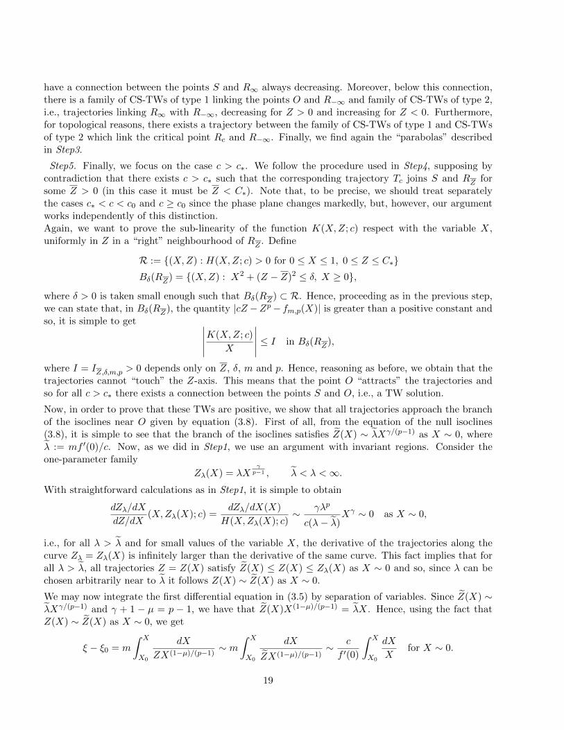
have a connection between the points S and R∞ always decreasing. Moreover, below this connection,there is a family of CS-TWs of type 1 linking the points O and R−∞ and family of CS-TWs of type 2,i.e., trajectories linking R∞ with R−∞, decreasing for Z > 0 and increasing for Z < 0. Furthermore,for topological reasons, there exists a trajectory between the family of CS-TWs of type 1 and CS-TWsof type 2 which link the critical point Rc and R−∞. Finally, we find again the “parabolas” describedin Step3.

Step5. Finally, we focus on the case c > c∗. We follow the procedure used in Step4, supposing bycontradiction that there exists c > c∗ such that the corresponding trajectory Tc joins S and RZ forsome Z > 0 (in this case it must be Z < C∗). Note that, to be precise, we should treat separatelythe cases c∗ < c < c0 and c ≥ c0 since the phase plane changes markedly, but, however, our argumentworks independently of this distinction.Again, we want to prove the sub-linearity of the function K(X,Z; c) respect with the variable X,uniformly in Z in a “right” neighbourhood of RZ . Define

R := (X,Z) : H(X,Z; c) > 0 for 0 ≤ X ≤ 1, 0 ≤ Z ≤ C∗Bδ(RZ) = (X,Z) : X2 + (Z − Z)2 ≤ δ, X ≥ 0,

where δ > 0 is taken small enough such that Bδ(RZ) ⊂ R. Hence, proceeding as in the previous step,we can state that, in Bδ(RZ), the quantity |cZ −Zp− fm,p(X)| is greater than a positive constant andso, it is simple to get ∣∣∣∣∣K(X,Z; c)

X

∣∣∣∣∣ ≤ I in Bδ(RZ),

where I = IZ,δ,m,p > 0 depends only on Z, δ, m and p. Hence, reasoning as before, we obtain that thetrajectories cannot “touch” the Z-axis. This means that the point O “attracts” the trajectories andso for all c > c∗ there exists a connection between the points S and O, i.e., a TW solution.

Now, in order to prove that these TWs are positive, we show that all trajectories approach the branchof the isoclines near O given by equation (3.8). First of all, from the equation of the null isoclines(3.8), it is simple to see that the branch of the isoclines satisfies Z(X) ∼ λXγ/(p−1) as X ∼ 0, whereλ := mf ′(0)/c. Now, as we did in Step1, we use an argument with invariant regions. Consider theone-parameter family

Zλ(X) = λXγp−1 , λ < λ <∞.

With straightforward calculations as in Step1, it is simple to obtain

dZλ/dX

dZ/dX(X,Zλ(X); c) =

dZλ/dX(X)

H(X,Zλ(X); c)∼ γλp

c(λ− λ)Xγ ∼ 0 as X ∼ 0,

i.e., for all λ > λ and for small values of the variable X, the derivative of the trajectories along thecurve Zλ = Zλ(X) is infinitely larger than the derivative of the same curve. This fact implies that forall λ > λ, all trajectories Z = Z(X) satisfy Z(X) ≤ Z(X) ≤ Zλ(X) as X ∼ 0 and so, since λ can bechosen arbitrarily near to λ it follows Z(X) ∼ Z(X) as X ∼ 0.

We may now integrate the first differential equation in (3.5) by separation of variables. Since Z(X) ∼λXγ/(p−1) and γ + 1 − µ = p − 1, we have that Z(X)X(1−µ)/(p−1) = λX. Hence, using the fact thatZ(X) ∼ Z(X) as X ∼ 0, we get

ξ − ξ0 = m

∫ X

X0

dX

ZX(1−µ)/(p−1) ∼ m∫ X

X0

dX

ZX(1−µ)/(p−1)∼ c

f ′(0)

∫ X

X0

dX

Xfor X ∼ 0.

19

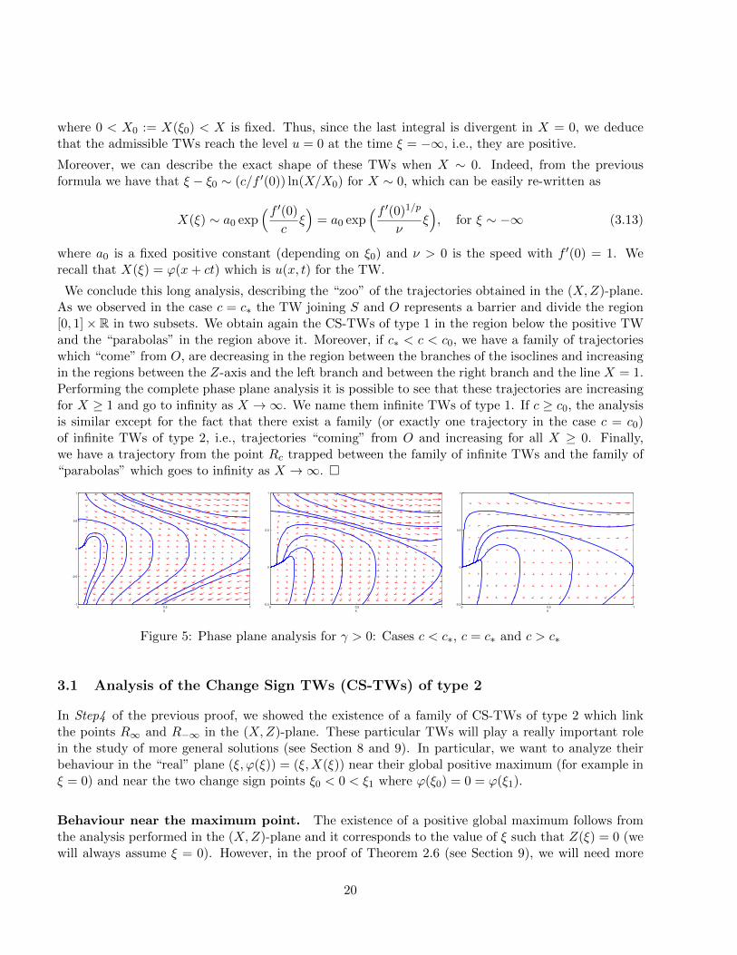
where 0 < X0 := X(ξ0) < X is fixed. Thus, since the last integral is divergent in X = 0, we deducethat the admissible TWs reach the level u = 0 at the time ξ = −∞, i.e., they are positive.

Moreover, we can describe the exact shape of these TWs when X ∼ 0. Indeed, from the previousformula we have that ξ − ξ0 ∼ (c/f ′(0)) ln(X/X0) for X ∼ 0, which can be easily re-written as

X(ξ) ∼ a0 exp(f ′(0)

cξ)

= a0 exp(f ′(0)1/p

νξ), for ξ ∼ −∞ (3.13)

where a0 is a fixed positive constant (depending on ξ0) and ν > 0 is the speed with f ′(0) = 1. Werecall that X(ξ) = ϕ(x+ ct) which is u(x, t) for the TW.

We conclude this long analysis, describing the “zoo” of the trajectories obtained in the (X,Z)-plane.As we observed in the case c = c∗ the TW joining S and O represents a barrier and divide the region[0, 1]× R in two subsets. We obtain again the CS-TWs of type 1 in the region below the positive TWand the “parabolas” in the region above it. Moreover, if c∗ < c < c0, we have a family of trajectorieswhich “come” from O, are decreasing in the region between the branches of the isoclines and increasingin the regions between the Z-axis and the left branch and between the right branch and the line X = 1.Performing the complete phase plane analysis it is possible to see that these trajectories are increasingfor X ≥ 1 and go to infinity as X →∞. We name them infinite TWs of type 1. If c ≥ c0, the analysisis similar except for the fact that there exist a family (or exactly one trajectory in the case c = c0)of infinite TWs of type 2, i.e., trajectories “coming” from O and increasing for all X ≥ 0. Finally,we have a trajectory from the point Rc trapped between the family of infinite TWs and the family of“parabolas” which goes to infinity as X →∞.

0 0,5 1-1

-0.5

0

0.5

1

X

0 0,5 1-0.5

0

0.5

1

X

0 0,5 1-0.5

0

0.5

1

X

Figure 5: Phase plane analysis for γ > 0: Cases c < c∗, c = c∗ and c > c∗

3.1 Analysis of the Change Sign TWs (CS-TWs) of type 2

In Step4 of the previous proof, we showed the existence of a family of CS-TWs of type 2 which linkthe points R∞ and R−∞ in the (X,Z)-plane. These particular TWs will play a really important rolein the study of more general solutions (see Section 8 and 9). In particular, we want to analyze theirbehaviour in the “real” plane (ξ, ϕ(ξ)) = (ξ,X(ξ)) near their global positive maximum (for example inξ = 0) and near the two change sign points ξ0 < 0 < ξ1 where ϕ(ξ0) = 0 = ϕ(ξ1).

Behaviour near the maximum point. The existence of a positive global maximum follows fromthe analysis performed in the (X,Z)-plane and it corresponds to the value of ξ such that Z(ξ) = 0 (wewill always assume ξ = 0). However, in the proof of Theorem 2.6 (see Section 9), we will need more

20

information on the CS-TWs near their maximum point when 0 < m < 1 and p > 2 (see relation (3.15)).So, with this choice of parameters, we differentiate with respect to the variable ξ the first equation in(3.5):

d2X

dξ2=

1

m

[(1− γ

p− 1

)X−γ/(p−1)

dX

dξZ +X1−γ/(p−1)dZ

dξ

]. (3.14)

Then, substituting the expressions in (3.5) and taking Z small, it is not difficult to see that

d2X

dξ2∼ −X

− γp−1 f(X)

m(p− 1)|Z|2−p, for Z ∼ 0.

In particular, for all 0 < X < 1 fixed, it is straightforward to deduce the relation we are interested in:∣∣∣∣dXdξ∣∣∣∣p−2∣∣∣∣d2Xdξ2

∣∣∣∣ ∼ m2−p

m(p− 1)Xp−2−γf(X) > 0, for Z ∼ 0, (3.15)

near the maximum point of ϕ = ϕ(ξ).

Behaviour near the change sign points. For what concerns the profile’s behaviour near zero, wecan proceed formally considering the equation of the trajectories (3.7) and observe that if X ∼ 0 andZ ∼ ∞ we have cZ − Zp − fm,p(X) ∼ −Zp and so

dZ

dX∼ − 1

(p− 1)

Z

Xi.e. Z ∼ a′X−

1p−1 , for X ∼ 0

for some a′ > 0. Now, from the first differential equation in (3.5), we get

dX

dξ∼ aX1−m, for X ∼ 0 (3.16)

where we set a = a′/m and integrating it between X = 0 and X = ϕ by separation of variables, we getthat the profile X = ϕ satisfies

ϕ(ξ) ∼ ma(ξ − ξ0)1/m for ξ ∼ ξ0 (3.17)

which not only explains us that the CS-TWs get to the level zero in finite time, but also tells us thatthey cannot be weak solutions of problem (1.1) since they violate the Darcy law: ϕ(ξ) ∼ (ξ− ξ0)γ/(p−1)near the free boundary (see [23], or [52] for the Porous Medium equation). For this reason they cannotdescribe the asymptotic behaviour of more general solutions, but they turn out to be really usefulwhen employed as “barriers” from below in the PDEs analysis. We ask the reader to note that, sincethe same procedure works when X ∼ 0 and Z ∼ −∞, we obtain the existence of the second point0 < ξ1 <∞ such that ϕ(ξ1) = 0 and, furthermore, the local analysis near ξ1 is similar.

Finally, using that Z ∼ aX−1/(p−1) for X ∼ 0, we can again obtain information on the behaviour ofthe second derivative near the change sign point ξ = ξ0. In particular, we get the relation

X2m−1d2X

dξ2∼ a2(p− 2− γ)

m2(p− 1)for X ∼ 0 and Z ∼ ∞, (3.18)

near the “free boundary point” of ϕ = ϕ(ξ). We will need this estimate in the proof of Theorem 2.6when in the case 0 < m < 1 and p > 2.

21

Detailed derivation of relation (3.16). Before, we deduced relation (3.16) in a too formal wayand we decided to end this section with a more complete proof. Let Z = Z(X) be a branch of thetrajectory of the CS-TW of type 2 and suppose Z ≥ 0 (the case Z ≤ 0 is similar).

Step1. We start proving that Z(X) ≥ aX−1/(p−1) for X ∼ 0 and some a > 0. Since, fm,p(X) ≥ 0 wehave

dZ

dX≤ cZ − Zp

(p− 1)XZp−1

which can be integrated by variable separation and gives Zp−1(X) ≥ −X0(c − Z0)p−1X−1, for all

0 < X ≤ X0 < 1 (X0 is the initial condition and Z0 = Z(X0)). Hence, taking X0 ∼ 0 and, consequently,Z0 ∼ ∞, we have that −X0(c− Z0)

p−1 ∼ X0Zp−10 and we deduce

Z(X) ≥ X1p−1

0 Z0X− 1p−1 for X ∼ 0.

Step2. Now, we show Z(X) ≤ aX−1/(p−1) for X ∼ 0. Using the fact that fm,p(X) ≤ Fm,p and Z ≥ 0,we get the differential inequality

dZ

dX≥ − Zp + Fm,p

(p− 1)XZp−1.

Proceeding as before, it is straightforward to deduce Zp ≤ Xp/(p−1)0 (Z0 + F )X−p/(p−1), where X0 and

Z0 are taken as before. Thus, since Xp/(p−1)0 (Z0 + F ) ∼ Xp/(p−1)

0 Z0 for X0 ∼ 0, we obtain

Z(X) ≤ X1p−1

0 Z0X− 1p−1 for X ∼ 0,

which allows us to conclude Z(X) ∼ aX−1p−1 for X ∼ 0 and a = X

1p−1

0 Z0 and, consequently, (3.16).

3.2 Continuity of the function c∗ for γ > 0

We end this section studying the continuity of the function c∗ = c∗(m, p) with respect the parametersm > 0 and p > 1, when γ > 0 (we prove the first step of Theorem 2.3). We will see that the continuityof the critical speed strongly depends on the stability of the orbit “entering” in the point S = (0, 1)(recall that we proved its existence and its uniqueness for all c > 0 in Step2 of Theorem 2.1). Beforeproceeding, we need to introduce the following notations:

• Zj = Zj(X) stands for the analytic representation of the trajectory Tc∗(mj ,pj) (as a function of X)for the values mj > 0 and pj > 1 such that γj = mj(pj − 1)− 1 > 0 and j = 0, 1.

• Aj = Aj(X) will indicate the analytic representation of the trajectories “above” Tc∗(mj ,pj), j = 0, 1.

• Bj = Bj(X) will indicate the analytic representation of the trajectories “below” Tc∗(mj ,pj), j = 0, 1.

The following lemma proves that the orbit Tc∗ is continuous with respect to the parameters m > 0 andp > 1.

Lemma 3.1 Let c = c∗. Then the orbit Tc∗ linking Rc∗ = (0, C∗) and S = (1, 0) is continuous withrespect to the parameters m > 0 and p > 1 (with γ > 0) uniformly on [0, 1].

This means that for all m0 > 0 and p0 > 1 with γ0 > 0, for all ε > 0 there exists δ > 0 such that

|Z0(X)− Z1(X)| ≤ ε for all |m0 −m1|+ |p0 − p1| ≤ δ with γ1 > 0

and for all 0 ≤ X ≤ 1.

22

Proof. Fix m0 > 0 and p0 > 1 with γ0 > 0 and note that the proof is trivial if X = 1.

Step1. First of all, we show that for all ε > 0 and for all 0 < X < 1, there exists δ > 0 such that

|Z0(X)− Z1(X)| ≤ ε for all |m0 −m1|+ |p0 − p1| ≤ δ with γ1 > 0.

So, fix 0 < X < 1 and ε > 0. We consider the trajectories A0 = A0(X) and B0 = B0(X) with

A0(X) = Z0(X) + ε and B0(X) = Z0(X)− ε, (3.19)

where Z0 = Z0(X), as we explained before, is the analytic expression for the trajectory Tc∗ withparameters m0 and p0. Since we proved that Tc∗ is “repulsive” near S (see Step2 of Theorem 2.1),we have that A0(·) has to cross the line Z = 1 in some point with positive height while B0(·) crossesthe X-axis in a point with first coordinate in the interval (X, 1). Hence, we can apply the continuityof the trajectories with respect to the parameters m and p outside the critical points and deduce theexistence of δ > 0 such that for all m1 and p1 satisfying |m0 − m1| + |p0 − p1| ≤ δ, the trajectoriesA1 = A1(X) and B1 = B1(X) with

A1(X) = Z0(X) + ε and B1(X) = Z0(X)− ε (3.20)

satisfy |A0(X)−A1(X)| ≤ ε and |B0(X)−B1(X)| ≤ ε for all X ≤ X ≤ 1. In particular, A1(·) crossesthe line Z = 1 in a point with positive height and B1(·) has to cross the X-axis in a point with firstcoordinate in the interval (X, 1). Consequently, since B1(X) ≤ Z1(X) ≤ A1(X) for all X ≤ X ≤ 1, wededuce that |Z0(X)− Z1(X)| ≤ ε.

Step2. Now, in order to show that

|Z0(X)− Z1(X)| ≤ ε for all X ≤ X ≤ 1,

we suppose by contradiction that there exists a point X < X′< 1 such that |Z0(X

′) − Z1(X

′)| > ε.

Without loss generality, we can suppose Z0(X′) > Z1(X

′) + ε. Then, we can repeat the procedure

carried out before by taking A0(·) and B0(·) satisfying (3.19) with X = X′. Hence, the continuity of

the trajectories with respect to the parameters m and p (outside the critical points) assures us the

existence of A1(·) and B1(·) satisfying (3.20) with X = X′. Hence, since B0(·) crosses the X-axis in

point with first coordinate in the interval (X′, 1) and B1(·) has to behave similarly (by continuity), we

have that the trajectory described by B1(·) and Z1(·) have to intersect, contradicting the uniquenessof the solutions.

We ask to the reader to note that, at this point, we have showed the continuity of the trajectory Tc∗with respect to the parameters m and p uniformly in the interval [X, 1], where 0 < X < 1 is arbitrary.

Step3. Finally, to conclude the proof, it is sufficient to check the continuity in X = 0, i.e., we have toprove that for all m0 > 0 and p0 > 1 such that γ0 > 0, for all ε > 0 there exists δ > 0 such that

|Z0(0)− Z1(0)| ≤ ε for all |m0 −m1|+ |p0 − p1| ≤ δ with γ1 > 0.

Arguing by contradiction again, we suppose that there exist ε > 0 such that for all δ > 0, we can findm1 and p1 with |m0 −m1|+ |p0 − p1| ≤ δ and γ1 > 0 such that it holds |Z0(0)− Z1(0)| > ε.

Hence, since the trajectories are continuous with respect to the variable X, we deduce the existence ofa small 0 < X < 1 such that |Z0(X)− Z1(X)| > ε/2 and so, thanks to the result from the Step1 andStep2, we can take δ > 0 small so that |Z0(X)−Z1(X)| ≤ ε/2, obtaining the desired contradiction.

23

A direct consequence of the previous lemma is the continuity of the function c∗ = c∗(m, p) in theregion H := (m, p) : γ = m(p− 1)− 1 > 0, that we enunciate in the following corollary.

Corollary 3.2 The function c∗ = c∗(m, p) is continuous in the region H, i.e., for all m0 and p0 withγ0 > 0 and for all ε > 0, there exists δ > 0 such that it holds |c∗(m0, p0)− c∗(m, p)| ≤ ε, for all m andp with γ > 0 and satisfying |m−m0|+ |p− p0| ≤ δ.

4 Existence of Travelling Wave solutions: case γ = 0

In this section, we address to problem of the existence of TW solutions for equation (2.3) in the“pseudo-linear” (limit) case γ = 0, i.e., m(p− 1) = 1. Note that the relation m(p− 1) = 1 generalizesthe linear setting m = 1 and p = 2 but the diffusion operator is still nonlinear. For this reason, theLiapunov’s linearization method cannot be applied and so we are forced to apply the same techniquesused in the proof of Theorem 2.1. However, as we will see in a moment, there are important differencesrespect to the case γ > 0 that have to be underlined: in particular, it turns out that the admissibleTWs are always positive while the TWs with free boundary disappear (see Theorem 2.2).

Proof of Theorem 2.2. We proceed as we did at the beginning of the previous proof, consideringthe equation of the profile (3.2) and performing the change of variable (3.4) which, in this case, can bewritten as

X = ϕ and Z = mϕ−1ϕ′ = mX−1X ′. (4.1)

Hence, we get the system

dX

dξ= (1/m)XZ, |Z|p−2 dZ

dξ= cZ − |Z|p −mX−1f(X), (4.2)

which can be re-written (after the re-parametrization dξ = |Z|p−2dτ) as the non-singular system

dX

dτ= (p− 1)X|Z|p−2Z, dZ

dτ= cZ − |Z|p − F (X), (4.3)

where F (X) := mX−1f(X) (note that F (0) = mf ′(0), F (1) = 0, F (X) ≥ 0 and F ′(X) ≤ 0 for all0 ≤ X ≤ 1).

System (4.3) possesses the critical point S = (1, 0) for all c ≥ 0. Now, define

c0∗(m, p) := p(m2f ′(0))1mp ,

as in (2.4). Then it is no difficult to prove:

• If c < c0∗(m, p), then there are no other critical points for system (4.3).

• If c = c0∗(m, p), then system (4.3) has another critical point Rλ∗ := (0, λ∗), where we define forsimplicity

λ∗ := (c0∗(m, p)/p)m = (m2f ′(0))1/p,

according to the definition of c0∗(m, p).

• If c > c0∗, then system (4.3) has also two critical points Rλi = (0, λi), i = 1, 2 where 0 < λ1 < λ∗ <λ2 < cm.

24

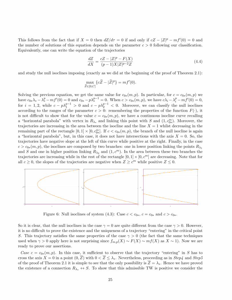
This follows from the fact that if X = 0 then dZ/dτ = 0 if and only if cZ − |Z|p −mf ′(0) = 0 andthe number of solutions of this equation depends on the parameter c > 0 following our classification.Equivalently, one can write the equation of the trajectories

dZ

dX=cZ − |Z|p − F (X)

(p− 1)X|Z|p−2Z(4.4)

and study the null isoclines imposing (exactly as we did at the beginning of the proof of Theorem 2.1):

maxZ∈[0,C]

cZ − |Z|p = mf ′(0).

Solving the previous equation, we get the same value for c0∗(m, p). In particular, for c = c0∗(m, p) wehave c0∗λ∗−λp∗−mf ′(0) = 0 and c0∗−pλp−1∗ = 0. When c > c0∗(m, p), we have cλi−λpi −mf ′(0) = 0,

for i = 1, 2, while c − pλp−11 > 0 and c − pλp−12 < 0. Moreover, we can classify the null isoclinesaccording to the ranges of the parameter c > 0: remembering the properties of the function F (·), itis not difficult to show that for the value c = c0∗(m, p), we have a continuous isocline curve recallinga “horizontal parabola” with vertex in Rλ∗ and linking this point with S and (1, cm0∗). Moreover, thetrajectories are increasing in the area between the isocline and the line X = 1 whilst decreasing in theremaining part of the rectangle [0, 1]× [0, cm0∗]. If c < c0∗(m, p), the branch of the null isocline is againa “horizontal parabola”, but, in this case, it does not have intersections with the axis X = 0. So, thetrajectories have negative slope at the left of this curve while positive at the right. Finally, in the casec > c0∗(m, p), the isoclines are composed by two branches: one in lower position linking the points Rλ1and S and one in higher position linking Rλ2 and (1, cm). In the area between these two branches thetrajectories are increasing while in the rest of the rectangle [0, 1]× [0, cm] are decreasing. Note that forall c ≥ 0, the slopes of the trajectories are negative when Z ≥ cm while positive Z ≤ 0.

0 10

0,5

1

X

Z

0 10

0.5

1

X

Z

0 10

0.5

1

X

Z

Figure 6: Null isoclines of system (4.3): Case c < c0∗, c = c0∗ and c > c0∗.

So it is clear, that the null isoclines in the case γ = 0 are quite different from the case γ > 0. However,it is no difficult to prove the existence and the uniqueness of a trajectory “entering” in the critical pointS. This trajectory satisfies the same properties of the case γ > 0 (the fact that the same techniquesused when γ > 0 apply here is not surprising since fm,p(X) ∼ F (X) ∼ mf(X) as X ∼ 1). Now we areready to prove our assertions.

Case c = c0∗(m, p). In this case, it sufficient to observe that the trajectory “entering” in S has tocross the axis X = 0 in a point (0, Z) with 0 < Z ≤ λ∗. Nevertheless, proceeding as in Step4 and Step5of the proof of Theorem 2.1 it is simple to see that the only possibility is Z = λ∗. Hence we have provedthe existence of a connection Rλ∗ ↔ S. To show that this admissible TW is positive we consider the

25

first differential equation in (4.2) and we integrate between X = 0 and X = 1 the equivalent differentialrelation dξ = (XZ)−1dX. It is straightforward to see that the correspondent integral is divergent bothnear X = 0 and X = 1, which means that the TW is positive.

Now we would like to describe the exact shape of this TW (with speed c0∗(m, p) := p(m2f ′(0))1mp )

as ξ ∼ −∞. In Step5 of Theorem 2.1, in the case γ > 0, we have given an analytic representationof the (positive) TWs corresponding to the value c > c∗(m, p). We found that the profile is a simpleexponential for ξ ∼ −∞, see formula (3.13). This has been possible since we have been able to describethe asymptotic behaviour of the trajectories in the (X,Z)-plane near X = 0. The case γ = 0 is morecomplicated and we devote Section 11 to the detailed analysis. Here, we simply report the asymptoticbehaviour of our TW ϕ = ϕ(ξ) with critical speed c0∗(m, p):

ϕ(ξ) ∼ a0|ξ|2p e

λ∗mξ = a0|ξ|

2p exp

(m

2−pp f ′(0)

1p ξ)

for ξ ∼ −∞, (4.5)

where λ∗ := (c0∗(m, p)/p)m = (m2f ′(0))1/p and a0 > 0.

We conclude this paragraph with a brief description of the remaining trajectories. Below the positiveTW, we have a family of trajectories linking Rλ∗ with R−∞ = (0,−∞) while above it, there are afamily of “parabolas” (exactly as in the case γ > 0). Between these two families, there are trajectoriesfrom the point Rλ∗ which cross the line X = 1.

Case c < c0∗(m, p). In this case there are not admissible TWs. Indeed, using again the same methodsof Step4 and Step5 it is simple to show that the orbit “entering” in S cannot touch the axis X = 0,i.e., it links R∞ = (0,∞) and S and so it is not an admissible TW. Below this trajectory there are afamily of CS-TWs of type 2 and above it we have a family of “parabolas”. We stress that, with thesame techniques used for the case γ > 0, the CS-TWs of type 2 satisfy Z(X) ∼ a′X−1/(p−1) = a′X−m

for X ∼ 0 and a suited positive constant a′. Hence, exactly as we did in Section 3, it is possible toshow that the profile X = ϕ reaches the level zero in to finite points −∞ < ξ0 < ξ1 < ∞. Indeed,exactly as we did before, using the first differential equation in (4.2), we get the estimate

dX

dξ∼ aX1−m for X ∼ 0,

from which we can estimate the (finite) times ξ0 and ξ1 (note that a = a′/m).

0 0,5 1-1

-0.5

0

0.5

1

X

Z

0 0.5 1-0.5

0

0.5

1

1.5

X

Z

0 0,5 1-1

-0.5

0

0.5

1

1.5

2

X

Z

Figure 7: Phase plane analysis for γ = 0: Cases c < c∗, c = c∗ and c > c∗

Case c > c0∗(m, p). To show the existence of a connection Rλ1 ↔ S and to prove that this TW ispositive, it is sufficient to apply the methods used in the case c = c0∗(m, p). We recall that for allc > c0∗(m, p), λ1 = λ1(c) < λ∗, it solves cλ1 − λp1 −mf ′(0) = 0, and c− pλp−11 > 0.

26

Now, by using the Lyapunov method, it is possible to linearize system (4.3) around the critical pointRλ1 = (0, λ1), and it is straightforward to see that its Jacobian matrix (calculated in (0, λ1)) has twopositive eigenvalues ν1 = (p − 1)λp−11 and ν2 = c − pλp−11 . This means that Rλ1 is a node unstable.Hence, we deduce that the trajectory Z = Z(X) from Rλ1 = (0, λ1) satisfies Z(X) ∼ λ1 − ν1X, forX ∼ 0 and we can re-write the first equation in (4.2) as

dX

dξ∼ (1/m)X(λ1 − ν1X) for X ∼ 0.

This is a first order logistic type ODE, and so we easily obtain that the profile X(ξ) = ϕ(x + ct) hasthe exponential decay

X(ξ) ∼ a0eλ1mξ, for ξ ∼ −∞, (4.6)

where a0 > 0 is a fixed constant.

Below this connection we have a family of trajectories joining Rλ1 and R−∞. Above it, there aretrajectories from Rλ2 and crossing the line X = 1, one trajectory from Rλ2 crossing the line X = 1and, finally, a family of “parabolas” as in the other cases.

Asymptotic behaviour of c0∗(m, p). We want to comment the asymptotic behaviour of the func-tion c0∗(m, p). Since we assume m(p − 1) = 1, it is simple to re-write the critical speed as a functionof m > 0 or p > 1:

c0∗(m) = (1 +m)m1−m1+m f ′(0)

1m+1 or c0∗(p) = p(p− 1)

− 2(p−1)p f ′(0)

p−1p .

Then we have:

limm→0

c0∗(m) = limp→∞

c0∗(p) = 0 and limm→∞

c0∗(m) = limp→1

c0∗(p) = 1.

These limits allow us to guess if in the cases m→ 0, p→∞ and m→∞, p→ 1 such that m(p−1) = 1,there exist TWs or not. It seems natural to conjecture that the answer is negative in the first case,while admissible TWs could exist in the second case.

0 1 2 10 200

1

2

2,5

m

c(m)

c = c

(m)

1 2 10 200

1

2

2,5

p

c(p)

c = c

(p)

Figure 8: Pseudo-linear case: the graphics of c0∗ in dependence of m > 0 and p > 1.

27

Finally, it is not difficult to calculate the derivative of c0∗(m) (or c0∗(p)) in the case f(u) = u(1− u):

c′0∗(m) = (m+ 1)−1m−2mm+1 (m+ 1− 2m logm)

and conclude that the maximum of the critical speed is assumed for a critical value of m = m∗, with2 < m∗ < 3 (of course, we can repeat this procedure with the function c0∗(p) finding a critical value4/3 < p∗ < 3/2). This simple calculation assures the the linear case m = 1 and p = 2 is not criticalfor the function c0∗(m, p) while the maximal speed of propagation is found choosing m = m∗ and/orp = p∗.

Remarks. We end the discussion on the value c0∗ in the “pseudo-linear” case with two observations.First of all, since the formulas for c∗(m) and c∗(p) depend on the value of f ′(0), it is always possible tomodify the reaction term f(·) with λf(·) for some λ > 0 (depending on m or p) and re-scale the spacevariable to have c0∗(m) = c0∗(p) = 1.

Secondly, we remind the reader to note that we obtained a value of c0∗(m, p) = p(m2f ′(0))1/(mp) whichgeneralizes the “classical one” (with m = 1 and p = 2) found in [6, 7] and [35], c∗ = 2

√f ′(0). Moreover,

it is interesting to see that our methods give an alternative and independent proof of the classical resultstated in Theorem 1.1.

4.1 Continuity of the function c∗ for γ ≥ 0

In these last paragraphs, we complete the proof of Theorem 2.3 showing the following lemma.

Lemma 4.1 The function defined in (2.5) is continuous in H, i.e., for all m0 and p0 with γ0 ≥ 0 andfor all ε > 0, there exists δ > 0 such that it holds |c0∗(m0, p0) − c∗(m, p)| ≤ ε, for all m and p withγ ≥ 0 and satisfying |m−m0|+ |p− p0| ≤ δ.

Proof. We divide the proof in some steps. In the first ones, we simply recall what we have showedearly.

Step1. First of all, we observe that, thanks to Corollary 3.2 and since the function c0∗(m, p) iscontinuous in the set γ = 0, it is sufficient to check the continuity along the boundary of the regionR. More precisely, we will show that for all m0 and p0 with γ0 = 0, for all ε > 0, there exists δ > 0 suchthat it holds |c0∗(m0, p0)−c∗(m, p)| ≤ ε, for all m and p with γ > 0 and satisfying |m−m0|+|p−p0| ≤ δ.

Step2. Now, we ask the reader to note that, with the same notations and techniques used in the proofof Lemma 3.1, it is possible to prove the continuity of the trajectory “entering” in S = (1, 0) withrespect to the parameters m and p with γ ≥ 0 uniformly in the variable X in all sets [X, 1], where Xis fixed in (0, 1]. This fact can be easily checked since, as we explained in the proof of Theorem 2.2,the local behaviour of the trajectories near the point S is the same for γ > 0 and γ = 0.

Step3. Before, proceeding with the proof we need to recall a last property. In the proof of Theorem2.1, we showed that c∗(m, p) < c0(m, p) for all m and p with γ > 0, where

c0(m, p) := p

(Fm,pp− 1

)(p−1)/p

,

and Fm,p is the maximum of the function fm,p(X) = mXγp−1−1f(X). Since fm,p(X) → mX−1f(X)

as γ → 0 for all 0 < X ≤ 1 and the limit function is decreasing, we have that the maximum point of

28

fm,p(·) converges to zero as γ → 0. Consequently, we obtain that Fm,p → mf ′(0) as γ → 0 and wededuce

c0(m, p)→ p(m2f ′(0))1/(m+1) = c0∗(m, p) as γ → 0.

Now we have all the elements needed for completing the proof by proving the assertion stated in Step1.

Step4. Suppose by contradiction that there exists m0 and p0 with γ0 = 0, ε > 0 and a sequence(mj , pj)→ (m0, p0) as j →∞ with γj > 0, such that |c0∗(m0, p0)− c∗(mj , pj)| ≥ ε for all j ∈ N.

Hence, there exists a subsequence that we call again c∗(mj , pj) converging to a value c 6= c0∗(m0, p0).Note that, since we proved c∗(mj , pj) < c0(mj , pj) → c0∗(m0, p0), it has to be c < c0∗(m0, p0) (seeStep3 ).

Now, since γj > 0, we have that the trajectory Tc∗(mj ,pj) joins the point S = (1, 0) with the point

Rc∗(mj ,pj) = (0, c∗(mj , pj)1/(pj−1)) for all j ∈ N and Rc∗(mj ,pj) → Rc = (0, c1/(p0−1)) as j → ∞. In

particular, it follows that the sequence of trajectories Tc∗(mj ,pj) has to be bounded. However, thanks tothe analysis done in the proof of Theorem 2.2, we know that if c < c0∗(m0, p0), the trajectory “entering”in the point S is unbounded and joins the previous point with R∞ = (0,∞). Consequently, applyingthe continuity of the trajectory “entering” in S with respect to the parameters m and p (stated inStep2 ) we obtain the desired contradiction and we conclude the proof.

5 Case γ > 0. Existence of minimal expanding super-level sets

From this moment on we address the question of the asymptotic analysis of general solutions. Moreprecisely, we devote five sections to the issue. In this section we prove Proposition 2.4 by appropriatelycombining a series of lemmas. As mentioned in the introduction, we study problem (1.1), with reactionterm f(·) satisfying (1.2) and with the particular choice of the initial datum:

u0(x) :=

ε if |x| ≤ %00 if |x| > %0,

(5.1)

where ε and %0 are positive real numbers. The choice of u0(·) in (5.1) is related to the finite propagationof the Barenblatt solutions in the case γ > 0 (see Section 2) and its usefulness will be clear in the nextsections (see Section 7).

We begin our study with an elementary lemma. Even though it has a quite simple proof, its meaningis important: it assures the existence of a (large) time such that the solution u = u(x, t) does notextinguish in time, but, on the contrary, remains larger than a (small) positive level, on all compactsets of RN .

Lemma 5.1 Let m > 0 and p > 1 such that γ > 0 and let N ≥ 1. Then for all 0 < ε < 1, for all%0 > 0 and for all %1 ≥ %0, there exists t1 > 0 and n1 ∈ N such that the solution u(x, t) of problem(1.1) with initial datum (5.1) satisfies

u(x, t1) ≥ ε/n1 in |x| ≤ %1.

Proof. Fix 0 < ε < 1 and 0 < %0 ≤ %1.We start with constructing a Barenblatt solution with positive parameters M1 and θ1 such thatBM1(x, θ1) ≤ u0(x) in RN . Since the profile of the Barenblatt solution is decreasing, we can choose

29

M1, θ1 > 0 such that BM1(0, θ1) = ε and BM1(x, θ1)||x|=%0 = 0. Thus, it is simple to obtain the relation

(Mγ1 θ1)

α = (k/C1)(p−1)N

p %N0 (5.2)

and the constants

θ1 = kp−1% p0 ε−γ and M1 = C

− p−1γ

1 (k/C1)(p−1)N

p %N0 ε, (5.3)

where C1 is the constant corresponding to the profile F1(·) and

α =1

γ + p/N, k =

γ

p

( αN

) 1p−1

are defined in Section 2. Then, we consider the solution of the problem∂tw = ∆pw

m in RN × (0,∞)

w(x, 0) = BM1(x, θ1) in RN ,

i.e., w(x, t) = BM1(x, θ1 + t), which satisfies u(x, t) ≥ w(x, t) in RN × (0,∞) thanks to the MaximumPrinciple (recall that by construction we have w(x, 0) ≤ u0(x)).

Now, we take t1 > 0 and n1 ∈ N satisfying

t1 ≥ 2N(p−1)αp θ1

(%1%0

)Nα

and n1 ≥ 2p−1γ

(1 +

t1θ1

)α. (5.4)

Thus, since the profile of the Barenblatt solutions is decreasing, in order to have u(x, t1) ≥ ε/n1 in|x| ≤ %1, it sufficient to impose

w(x, t1)||x|=%1 = BM1(x, θ1 + t1)||x|=%1 ≥ ε/n1. (5.5)

Now, using the relations in (5.2) and (5.3), it is not difficult to compute

BM1(x, θ1 + t1)||x|=%1 = M1B1(x,Mγ1 (θ1 + t1))||x|=%1

=M1

(Mγ1 θ1)

α

(θ1

θ1 + t1

)αC1 − k

(%1%0

) pp−1

[(Mγ

1 θ1)− αN

(θ1

θ1 + t1

) αN] pp−1 p−1

γ

+

= ε

(θ1

θ1 + t1

)α[1−

(%1%0

) pp−1

(θ1

θ1 + t1

) αpN(p−1)

] p−1γ

+

.

So, requiring (5.5) is equivalent to[1−

(θ1

θ1 + t1

) αpN(p−1)( %1

%0

) pp−1

] p−1γ

+

≥ 1

n1

(1 +

t1θ1

)α. (5.6)

Since the first condition in (5.4) assures that the term on the left side of the previous inequality islarger than 2−(p−1)/γ , we have that a sufficient condition so that (5.6) is satisfied is

n1 ≥ 2p−1γ

(1 +

t1θ1

)α,

30

which is our second assumption in (5.4), and so our proof is complete.

We proceed in our work, proving that, for all ε > 0 small enough, the super-level sets E+ε (t) := x ∈

RN : u(x, t) ≥ ε of the solution u = u(x, t) of problem (1.1) with initial datum (5.1) do not contractin time for t large enough and, in particular, we will show that for all m > 0 and p > 1 such that γ > 0and for all %0 > 0, it holds

|x| ≤ %0/2 ⊂ E+ε (t), for large times.

This result highlights the role of the reaction term f(·). Indeed, the solution of the “pure diffusive”equation converges to zero as t→∞, whilst the presence of the function f(·) is sufficient to guaranteethe strict positivity of the solution in a (small) compact set for large times.

Lemma 5.2 Let m > 0 and p > 1 such that γ > 0 and let N ≥ 1. Then, for all %0 > 0, there existt2 > 0 and 0 < ε0 < 1 which depend only on m, p, N , f and %0, such that for all 0 < ε ≤ ε0, thesolution u(x, t) of problem (1.1) with initial datum (5.1) satisfies

u(x, jt2) ≥ ε in |x| ≤ %0/2, for all j ∈ N+ = 1, 2, . . ..

Proof. We prove the assertion by induction on j ∈ N+. We ask the reader to note that we follow theideas previously used by Cabre and Roquejoffre [10] and, later, in [48] adapting them to our (quitedifferent) setting.

Step0. In this step, we introduce some basic definitions and quantities we will use during the proof.

We fix j = 1 and %0 > 0. Moreover, let 0 < δ < 1 and set λ := f(δ)/δ. Then take t2 large enough suchthat

eλt2 ≥ 2p−1γ

(1 +

τ(t2)

C1

)α(5.7)

where α > 0 and k > 0 are defined in Section 2 (see also the beginning of the proof of Lemma 5.1).The constant C1 is defined by the formula

C1 := kp−1% p0

and the function τ(·) is defined as follows:

τ(t) =1

γλ

[eγλt − 1

], for t ≥ 0. (5.8)

Then, we set ε0 := δe−f′(0)t2 and, finally, we fix 0 < ε ≤ ε0. Note that the choices in (5.7) are admissible

since γα < 1 and t2 > 0 does not depend on ε.

Step1. Construction of a sub-solution of problem (1.1), (5.1) in RN × [0, t2].First of all, as we did at the beginning of the proof of Lemma 5.1, we construct a Barenblatt solutionof the form BM1(x, θ1) such that BM1(x, θ1) ≤ u0(x) for all x ∈ RN . Evidently, we obtain the sameformulas for M1 > 0 and θ1 > 0 (see (5.2) and (5.3)). Before proceeding, we note that, using (5.3) andthe fact that ε < 1, it is simple to get

θ1 ≥ C1 > 0. (5.9)

Now, consider the change of time variable τ = τ(t) defined in (5.8) and the “linearized” problem∂tw = ∆pw

m + λw in RN × (0,∞)

w(x, 0) = u0(x) in RN .(5.10)

31

Then, the function w(x, τ) = e−λtw(x, t) solves the problem∂τ w = ∆pw

m in RN × (0,∞)

w(x, 0) = u0(x) in RN .

Since BM1(x, θ1) ≤ u0(x) ≤ ε for all x ∈ RN , from the Maximum Principle we get

BM1(x, θ1 + τ) ≤ w(x, τ) ≤ ε in RN × (0,∞). (5.11)

Hence, using the concavity of f and the second inequality in (5.11) we get

w(x, t) = eλtw(x, τ) ≤ εef ′(0)t ≤ ε0ef′(0)t2 = δ, in RN × [0, t2]

and so, since w ≤ δ implies f(δ)/δ ≤ f(w)/w, we have that w is a sub-solution of problem (1.1), (5.1)in RN × [0, t2]. Finally, using the first inequality in (5.11), we obtain

u(x, t) ≥ eλtw(x, τ) ≥ eλtBM1(x, θ1 + τ), in RN × [0, t2]. (5.12)

Step2. In this step, we verify that the assumptions (5.7) on t2 > 0 (depending only on m, p, N , fand %0) are sufficient to prove u(x, t2) ≥ ε in the set |x| ≤ %0/2.First of all, we note that, from the second inequality in (5.12) and since the profile of the Barenblattsolution is decreasing, it is clear that it is sufficient to have t2 such that

eλt2BM1(x, θ1 + τ2)||x|=%0/2 ≥ ε, (5.13)

where τ2 := τ(t2). Using the relations in (5.2) and (5.3) and proceeding as in the proof of Lemma 5.1,we get

eλt2BM1(x, θ1 + τ2)||x|=%0/2 = ε eλt2

(θ1

θ1 + τ2

)α[1− 2

− pp−1

(θ1

θ1 + τ2

) αpN(p−1)

] p−1γ

+

Hence, we have that (5.13) is equivalent to

eλt2

[1− 2

− pp−1

(θ1

θ1 + τ2

) αpN(p−1)

] p−1γ

+

≥

(1 +

τ2θ1

)α. (5.14)

Since for all fixed τ > 0, the function θ/(θ + τ) satisfies

θ

θ + τ≤ 1 ≤ 2

Nαp , for all θ ≥ 0

and since θ1 ≥ C1 (see (5.9)), it is simple to deduce that a sufficient condition so that (5.14) is satisfiedis

eλt2 ≥ 2p−1γ

(1 +

τ2

C1

)αNote that it does not depend on 0 < ε ≤ ε0 and it is exactly the assumption (5.7) on t2 > 0. The proofof the case j = 1 is completed.

32

However, before studying the iteration of this process, we need to do a last effort. Let %1 ≥ %0/2 besuch that

eλt2BM1(x, θ1 + τ2)||x|=%1 = ε

and introduce the function

v0(x) :=

ε if |x| ≤ %1eλt2BM1(x, θ1 + τ2) if |x| > %1.

A direct computation (which we leave as an exercise for the interested reader) shows that condition(5.7) is sufficient to prove

u(x, t2) ≥ v0(x) ≥ BM1(x, θ1) in RN . (5.15)

Iteration. We suppose to have proved that the solution of problem (1.1), (5.1) satisfies

u(x, jt2) ≥ ε in |x| ≤ %0/2, for some j ∈ N+

with the propertyu(x, jt2) ≥ v0(x) ≥ BM1(x, θ1) in RN (5.16)

which we can assume since it holds in the case j = 1 (see (5.15)) and we prove

u(x, (j + 1)t2) ≥ ε in |x| ≤ %0/2. (5.17)

Thanks to (5.16), it follows that the solution v(x, t) of the problem∂tv = ∆pv

m + f(v) in RN × (0,∞)

v(x, 0) = v0(x) in RN(5.18)

satisfies u(x, t+ jt2) ≥ v(x, t) in RN × [0,∞) by the Maximum Principle. Consequently, we can workwith the function v(x, t) and proceeding similarly as before.

Step1’. Construction of a sub-solution of problem (5.18) in RN × [0, t2].This step is identical to Step1 (case j = 1). However, we ask the reader to keep in mind that now weare building a sub-solution of the function v = v(x, t). This means that we consider the “linearized”problem

∂tw = ∆pwm + λw in RN × (0,∞)

w(x, 0) = v0(x) in RN

where λ := f(δ)/δ and, using again the change of variable (5.8), we deduce that the function w(x, τ) =e−λtw(x, t) solves the problem

∂τ w = ∆pwm in RN × (0,∞)

w(x, 0) = v0(x) in RN .

Since BM1(x, θ1) ≤ v0(x) ≤ ε for all x ∈ RN , from the Maximum Principle we get again

BM1(x, θ1 + τ) ≤ w(x, τ) ≤ ε in RN × (0,∞)

33

and, moreover, w(x, t) ≤ δ in RN × [0, t2] which allows us to conclude that w = w(x, t) is a sub-solutionof problem (5.18) in RN × [0, t2]. In particular, it holds

u(x, (j + 1)t2) ≥ v(x, t2) ≥ w(x, t2) ≥ eλt2BM1(x, θ1 + τ2).

Step2’. This step is identical to Step2, since we have to verify that

eλt2BM1(x, θ1 + τ2)||x|=%0/2 ≥ ε.

Since we showed in Step2 that (5.7) is as sufficient condition so that the previous inequality is satisfied,we obtain (5.17) and we conclude the proof.

However, in order to be precise and be sure that our iteration actually works, we have to prove that

u(x, (j + 1)t2) ≥ BM1(x, θ1) in RN ,

but this follows from the fact that w(x, t2) ≥ v0(x) ≥ BM1(x, θ1) in RN .

Corollary 5.3 Let m > 0 and p > 1 such that γ > 0 and let N ≥ 1. Then, there exist t2 > 0 and0 < ε0 < 1 which depend only on m, p, N , f and %0 such that, for all 0 < ε ≤ ε0, the solution u(x, t)of problem (1.1) with initial datum (2.6) satisfies

u(x, t) ≥ ε in |x| ≤ %0/2 for all t ≥ t2.

Proof. The previous lemma states that for all %0 > 0 and for the sequence of times tj = (jt2)j∈N+ , thesolution of problem (1.1), (5.1) reaches a positive value ε in the set |x| ≤ %0/2, i.e.

u(x, jt2) ≥ ε in |x| ≤ %0/2, for all j ∈ N+,

for all 0 < ε ≤ ε0 = δe−f′(0)t2 . We can improve this result choosing a smaller ε0 > 0.

Indeed, since conditions (5.7):

eλt2 ≥ 2(p−1)γ

(1 +

τ(t2)

C1

)αare satisfied for all t2 ≤ t ≤ 2t2, we can repeat the same proof of Lemma 5.2, modifying the valueof ε0 and choosing a different value ε0 = δe−2f

′(0)t2 > 0, which is smaller but strictly positive for allt2 ≤ t ≤ 2t2. Hence, it turns out that for all 0 < ε ≤ ε0, it holds

u(x, t) ≥ ε in |x| ≤ %0/2, for all t2 ≤ t ≤ 2t2.

Now, iterating this procedure as in the proof of Lemma 5.2, we do not have to change the value of ε0when j ∈ N+ grows and so, for all 0 < ε ≤ ε0, we obtain

u(x, t) ≥ ε in |x| ≤ %0/2, for all j ∈ N+ and for all jt2 ≤ t ≤ (j + 1)t2.

Hence, using the arbitrariness of j ∈ N+, we end the proof of this corollary.

Now, in order to prove our main instrument (Proposition 2.4), needed in the study of the asymptoticbehaviour of the general solutions of problem (1.1) (see Lemma 7.1), we combine Lemma 5.1 andCorollary 5.3.

34

Proof of Proposition 2.4 (case γ > 0). Fix %0 > 0, %1 ≥ %0 and consider the solution u = u(x, t)of problem (1.1) with initial datum (5.1). So, thanks to Lemma 5.1, for all 0 < ε1 < 1, there existt1 > 0 and n1 ∈ N such that

u(x, t1) ≥ ε := ε1/n1 in |x| ≤ %1.

Now, define the function

v0(x) :=

ε if |x| ≤ %10 if |x| > %1

and note that u(x, t1) ≥ v0(x) in RN . Hence, the solution of the problemvt = ∆pv

m + f(v) in RN × (0,∞)

v(x, 0) = v0(x) in RN

satisfies u(x, t1 + t) ≥ v(x, t) in RN × (0,∞). Finally, applying Corollary 5.3, we get

u(x, t) ≥ ε in |x| ≤ %1/2 for all t ≥ t0

with t0 := t1 + t2 (note that, since n1 ∈ N can be chosen larger, ε > 0 is arbitrarily small and we “endup” in the hypotheses of Corollary 5.3).

6 Case γ = 0. Existence of minimal expanding super-level sets

In this section we study problem (1.1), with reaction term f(·) satisfying (1.2) and with initial datum:

u0(x) :=

ε if |x| ≤ %0

a0e−b0|x|

pp−1

if |x| > %0,a0 := εeb0%

pp−10 (6.1)

where ε, %0 and b0 are positive numbers (note that u0 ∈ L1(RN )). We ask the reader to note that,alternatively, we can fix the constants %0, a0 and b0 and obtaining ε > 0 by the “inverse” of the secondformula in (6.1).

Our goal is to prove Proposition 2.4. Anyway, in order to motivate our choice from the beginning, westart proving the following lemma which will be useful in the proof of Lemma 7.1.

Lemma 6.1 Let m > 0 and p > 1 such that γ = 0 and let N ≥ 1. Then for all %0 > 0, there existt1 > 0, a0 > 0 and b0 > 0 such that the solution u(x, t) of problem (1.1) with initial datum (1.3)satisfies

u(x, t1) ≥ u0(x) in RN

where u0(·) is defined in (6.1).

Proof. Let u = u(x, t) the solution of problem (1.1), (1.3) and consider the solution v = v(x, t) of the“pure diffusive” Cauchy problem:

∂tv = ∆pvm in RN × (0,∞)

v(x, 0) = u0(x) in RN ,

35

which satisfies v(x, t) ≤ u(x, t) in RN × [0,∞) thanks to the Maximum Principle.

Step1. We begin by proving that for all τ > 0, there exist ε > 0, M > 0 such that for all τ < t1 < τ+εit holds

u(x, t1) ≥ BM (x, t1 − τ) in RN

where BM (x, t) is the Barenblatt solution in the “pseudo-linear” case (presented in Section 2) withexponential form

BM (x, t) = CM t−Np exp

(− k|xt−

1p |

pp−1

),

where CM > 0 is chosen depending on the mass M and k = (p− 1)p−p/(p−1).

Fix τ > 0, % > 0 and let ε > 0 (for the moment arbitrary). Furthermore, take a mass M > 0 such thatCM ≤ 1. We want to compare the general solution v = v(x, t) with the “delayed” Barenblatt solutionBM = BM (x, t− τ) in the strip

S = [τ, τ + ε]× x ∈ RN : |x| ≥ %,

in order to deduce v(x, t) ≥ BM (x, t − τ) in S. Hence, from the Maximum Principle, is sufficient tocheck this inequality on the parabolic boundary of S. Note that we have v(x, τ) ≥ BM (x, 0) = 0 forall |x| ≥ %. Now, in order to check that v(%, t) ≥ BM (%, t − τ) for all τ ≤ t ≤ τ + ε, we compute thederivative of the function b(t) := BM (%, t− τ) deducing that

b′(t) ≥ 0 if and only if t ≤ τ +

[pk

N(p− 1)

]p−1% p.

Thus, choosing ε ≤ (pk)/[N(p − 1)]p−1% p and noting that v(%, t) ≥ v > 0 for all τ ≤ t ≤ τ + εand some constant v > 0 (the strict positivity follows from the Harnack Inequality proved in [34]), wehave that it is sufficient to prove v ≥ BM (%, ε). Since, BM (%, ε)→ 0 as ε→ 0, we obtain the requiredinequality by taking eventually ε > 0 smaller. We ask to the reader to note that the assumptionCM ≤ 1 guarantees that the choice of ε > 0 does not depend on M > 0.

Now, take τ < t1 < τ+ε. We know v(x, t1) ≥ BM (x, t1−τ) if |x| ≥ % and so, by taking CM > 0 smaller(depending on ε > 0) and using again the positivity of the solution v = v(x, t), it is straightforward tocheck that the same inequality holds for all |x| ≤ %, completing the proof of the first step.

Step2. Fix %0 > 0 and let t1 > 0 be fixed as in the previous step. To end the proof, it is sufficient toprove

BM (x, t1 − τ) ≥ u0(x) in |x| ≥ %0,

since the profile of the Barenblatt solution is radially decreasing. A direct computation shows that theprevious inequality is satisfied by taking

a0 ≤ CM (t1 − τ)−N/p and b0 ≥ k(t1 − τ)−1/(p−1)

and so, the proof is complete.

Following the ideas of the previous section (see Lemma 5.2), we prove that for all ε > 0 small enough,the super-level sets E+

ε (t) of the solution u = u(x, t) of problem (1.1) with initial datum (6.1) expandin time for t large enough. More precisely, we will show that for all %0 > 0 and for all %1 ≥ %0, it holds

|x| ≤ %1 ⊂ E+ε (t), for large times.

36

This will result a slightly simpler respect to the case γ > 0, since now we work with strictly positiveBarenblatt solutions (see Section 2). For instance, we do not need a version of Lemma 5.1, which seemsto be essential in the case γ > 0.

Lemma 6.2 Let m > 0 and p > 1 such that γ = 0 and let N ≥ 1. Then, for all %0 > 0 and for all%1 ≥ %0, there exist t0 > 0 and 0 < ε0 < 1 which depend only on m, p, N , f , u0 and %1, such that forall 0 < ε ≤ ε0, the solution u(x, t) of problem (1.1) with initial datum (6.1) satisfies

u(x, jt0) ≥ ε in |x| ≤ %1, for all j ∈ N+ = 1, 2, . . ..

Proof. We prove the assertion by induction on j = 1, 2, . . . .

Step0. As in the proof of Lemma 5.2, this “first” step is devoted to the introduction of basic definitionsand quantities we need during the proof.

We fix j = 1, %0 > 0 and %1 ≥ %0. Moreover, let 0 < δ < 1, set λ := f(δ)/δ and fix 0 < λ0 < λ. Thentake t0 large enough such that

t0 ≥ kp−1% p1 , eλ0t0 ≥(θ1 + t0θ1

)N/pand t0 ≥

1

λ− λ0(6.2)

and, furthermore:

t0 ≥(

2k

b0

)p−1and t0 ≥

b02(λ− λ0)

%pp−1

1 (6.3)

where (we ask the reader to note that we defined k in Section 2, case γ = 0):

k := (p− 1)p−p/(p−1) and θ1 :=

(k

b0

)p−1.

Then, we set ε0 := δe−f′(0)t0 and, finally, we fix 0 < ε ≤ ε0.

Step1. Construction of a sub-solution of problem (1.1), (6.1) in RN × [0, t0].First of all, as we did at the beginning of the proof of Lemma 5.1 and Lemma 5.2, we construct aBarenblatt solution of the form BM1(x, θ1) such that BM1(x, θ1) ≤ u0(x) for all x ∈ RN . Note thatin the case γ = 0, the Barenblatt solutions have exponential profile (see Section 2). Imposing again

BM1(0, θ1) = ε we get the first relation CM1θ−N/p1 = ε which is sufficient to have BM1(x, θ1) ≤ u0(x)

in |x| ≤ %0. On the other hand, for all |x| ≥ %0, we need to have:

BM1(x, θ1) ≤ a0e−b0|x|pp−1

, |x| ≥ %0.

Using the relation CM1θ−N/p1 = ε and the fact that ε ≤ a0, it is not difficult to see that a possible

choice of parameters such that the previous inequality is satisfied too is

θ1 =

(k

b0

)p−1and CM1 = ε

(k

b0

)N(p−1)p

. (6.4)

Note that, respect to the case γ > 0, θ1 does not depend on ε > 0. Now, as in the proof of Lemma 5.2,we consider the “linearized” problem

∂tw = ∆pwm + λw in RN × (0,∞)

w(x, 0) = u0(x) in RN(6.5)

37

and we deduce that the function w(x, t) = e−λtw(x, t) solves the problem (note that when when γ = 0the doubly nonlinear operator has homogeneity 1)

∂tw = ∆pwm in RN × (0,∞)

w(x, 0) = u0(x) in RN .

Again we have that BM1(x, θ1) ≤ u0(x) ≤ ε for all x ∈ RN and so, by comparison we deduce

BM1(x, θ1 + t) ≤ w(x, t) ≤ ε in RN × (0,∞). (6.6)

Hence, using the concavity of f and the second inequality in (6.6) we get

w(x, t) = eλtw(x, t) ≤ εef ′(0)t ≤ ε0ef′(0)t0 = δ, in RN × [0, t0]

and, consequently, w = w(x, t) is a sub-solution of problem (1.1), (6.1) in RN × [0, t0]. Finally, usingthe first inequality in (6.6), we obtain

u(x, t) ≥ eλtBM1(x, θ1 + t), in RN × [0, t0]. (6.7)

Step2. In this step, we verify that the assumptions (6.2) on t0 > 0 are sufficient to prove u(x, t0) ≥ εin the set |x| ≤ %1.First of all, we note that, from the second inequality in (6.7) and since the profile of the Barenblattsolution is decreasing, it is clear that it is sufficient to have t0 such that

eλt0BM1(x, θ1 + t0)||x|=%1 ≥ ε. (6.8)

Using the relations, we compute

eλt0BM1(x, θ1 + t0)||x|=%1 = ε

(θ1

θ1 + t0

)N/pexp

[λt0 − k

(% p1

θ1 + t0

)1/(p−1)].

Hence, we have that (6.8) is equivalent to(θ1

θ1 + t0

)N/pexp

[λt0 − k

(% p1

θ1 + t0

)1/(p−1)]≥ 1. (6.9)

Now, using the first and the second relation in (6.2) it is not difficult to see that a sufficient conditionso that (6.9) is satisfied is

e(λ−λ0)t0−1 ≥ 1,

which is equivalent to the third assumption in (6.2) and so, we have u(x, t0) ≥ ε in |x| ≤ %1, i.e. thethesis for j = 1.

As we did in Lemma 5.2, we have to do a last step in order to conclude the case j = 1. Let %2 ≥ %1such that

eλt0BM1(x, θ1 + t0)||x|=%2 = ε.

Evidently, defining the function:

v0(x) :=

ε if |x| ≤ %2eλt0BM1(x, θ1 + t0) if |x| > %2,

38

it is sufficient to prove v0(x) ≥ BM1(x, θ2) in |x| > %1 and, using the second relation in (6.2), it issimple to see that this is automatically satisfied if

exp[(λ− λ0)t0

]≥ exp

[b0%

pp−1

0 + (kt− 1p−1

0 − b0)|x|pp−1].

Now, keeping in mind that %1 ≥ %0 and using the first inequality in (6.3), we deduce that a sufficientcondition so that the previous inequality is satisfied is

e(λ−λ0)t0 ≥ e(b0/2)%pp−11 ,

which is equivalent to the second condition in (6.3). Hence, we have

u(x, t0) ≥ v0(x) ≥ BM1(x, θ1) in RN . (6.10)

Iteration. We suppose to have proved that the solution of problem (1.1), (6.1) satisfies

u(x, jt0) ≥ ε in |x| ≤ %1, for some j ∈ N+

with the propertyu(x, jt0) ≥ v0(x) ≥ BM1(x, θ1) in RN (6.11)

and we proveu(x, (j + 1)t0) ≥ ε in |x| ≤ %1.

As in the proof of Lemma 5.2, we have that (6.11) implies that the solution v = v(x, t) of the problemvt = ∆pv

m + f(v) in RN × (0,∞)

v(x, 0) = v0(x) in RN(6.12)

satisfies u(x, t + jt0) ≥ v(x, t) in RN × [0,∞) by the Maximum Principle and this allows us to workwith the function v = v(x, t). The rest of the proof is almost identical to the case γ > 0 (see Lemma5.2) and we leave the details to the interested reader.

Proof of Proposition 2.5 (case γ = 0). The proof is identical to the proof of Corollary 5.3,substituting condition (5.7) with conditions (6.2) and (6.3), %0/2 with %1 and t2 with t0.

7 Asymptotic behaviour. Convergence to 1 on compact sets

In this section, we prove a technical lemma (see Lemma 7.1) which will be crucial in the study ofthe asymptotic behaviour of the solution of the Cauchy problem (1.1), (1.3) with reaction term f(·)satisfying (1.2). We make the additional assumption u0(0) = maxx∈R u0(x) (note that this choice isclearly admissible by performing a translation of the x-axis and it will avoid tedious technical work inthe rest of the section).

In what follows, we show that a general solution (for all γ ≥ 0) converges to one on every compact setof RN (“large enough”) for large times.

39

Lemma 7.1 Let m > 1 and p > 1 such that γ ≥ 0 and let N ≥ 1. Then, for all ε > 0, there exist0 < aε < 1 and %ε > 0 (which depend on ε > 0) such that for all %1 ≥ %ε, there exists t1 > 0 (dependingon %1, ε) such that it holds

u(x, t) ≥ 1− ε in |x| ≤ aε%1, for all t ≥ t1.

Proof. We begin supposing γ > 0. Fix ε > 0.

Step1. In this step, we construct a sub-solution of problem (1.1) on a domain of the form Ω× (t1,∞),where Ω is a ball in RN and t1 > 0.First of all, we fix %2 = 2%1 > 0 arbitrarily large and we apply Proposition 2.4 deducing the existenceof a value ε > 0 and a time t0 > 0 such that

u(x, t) ≥ ε in Ω× [t0,∞)

where Ω := |x| ≤ %1. Hence, since ε ≤ u ≤ 1 and remembering that the function f(·) is concave, wecan deduce a linear bound from below for the reaction term

f(u) ≥ q(1− u) in Ω× [t0,∞), where q := f(ε)/(1− ε).

Now, for all %1 > 0, we consider a time t1 ≥ t0 (note that t1 is now “almost” arbitrary and its precisevalue depending on ε > 0 will be specified later). Thus, the solution of the problem

∂tv = ∆pvm + q(1− v) in Ω× (t1,∞)

v = ε in ∂Ω× (t1,∞)

v(x, t1) = ε in Ω

(7.1)

satisfies ε ≤ v(x, t) ≤ u(x, t) ≤ 1 in Ω× [t1,∞) by the Maximum Principle. Furthermore, since for allfixed τ > 0, the function w(x, t) = v(x, τ + t) satisfies the equation in (7.1) and w(x, t1) ≥ v(x, t1),it follows v(x, τ + t) ≥ v(x, t) in Ω × [t1,∞), i.e., for all x ∈ Ω, the function v(x, ·) is non-decreasing.Consequently, since v is uniformly bounded, there exists the uniform limit v∞(x) := limt→∞ v(x, t) andit solves the elliptic problem

−∆pvm∞ = q(1− v∞) in Ω

v∞ = ε in ∂Ω(7.2)

in the weak sense.

Step2. In this step, we define the constants aε and %ε and we complete the proof of the lemma. Thevalue of these constants comes from the construction of a particular sub-solution of the elliptic problem(7.2). Since our argument is quite technical, we try to sketch it skipping some computations that canbe verified directly by the reader.

We look for a sub-solution of the elliptic problem (7.2) in the form

wm(r) = a[eg(r) − 1

],

where r = |x|, x ∈ RN while the function g(·) and the constant a > 0 are taken as follows:

g(r) := 1−(r

%1

)λ, with λ :=

p

p− 1and

(1− ε/2)m

e− 1< a <

1

e− 1.

40

Note that the radially decreasing function w(·) is well defined in [0, %1] and, moreover, w(r) = 0 on theboundary ∂Ω = |x| = %1.Now, we define the value %ε (note it is well defined and positive thanks to the assumption on a) withthe formula

% pε :=N(aeλ)p−1

q1− [a(e− 1)]1/mand we show that for all %1 ≥ %ε, w(·) is a sub-solution of the equation in (7.2). Note that, since w(·)is radially decreasing, it is sufficient to consider our operator (the p-Laplacian) in radial coordinatesand verify that for all %1 ≥ %ε and 0 ≤ r ≤ %1, it holds

−∆p,rwm := −r1−N∂r(rN−1|∂rwm|p−2∂rwm) ≤ q(1− w). (7.3)

A direct computation shows that

−∆p,rwm =

(aλ

%λ1

)p−1[N − p(r/%1)λ

]e(p−1)g(r)

and that sufficient condition so that inequality (7.3) is satisfied is

N(aeλ)p−1%−p1 ≤ q1− [a(e− 1)]1/m,

which is equivalent to say %1 ≥ %ε. Finally, we define aε with the formula:

aλε := 1− log

[a+ (1− ε/2)m

a

].

It is not difficult to see that w(r) ≥ 1−ε/2 in r ≤ aε%1 and that again our assumption on a guaranteethe well definition of aε.

Hence, if we suppose %1 ≥ %ε, we can apply the elliptic Maximum Principle (recall that w = 0 on theboundary ∂Ω) deducing

v∞(x) ≥ 1− ε/2 in |x| ≤ aε%1.

So, since v(x, t) → v∞(x) as t → ∞, a similar inequality holds for the function v = v(x, t) and largetimes:

v(x, t) ≥ 1− ε in |x| ≤ aε%1, for all t ≥ t1where t1 > 0 is chosen large enough (depending on ε > 0) and the same conclusion is true for thesolution u = u(x, t) of problem (1.1) since it holds v(x, t) ≤ u(x, t) in Ω× [t1,∞).

As the reader can easily check, the proof when γ = 0 is identical to the case γ > 0 except for the factthe we apply Proposition 2.5 instead of Proposition 2.4 (see also the following remark).

Remark. At the beginning of Step1 (case γ > 0), we have applied Proposition 2.4, even though theassumptions (1.3) on u0 are not sufficient to guarantee its hypotheses. However, it is really simple tosee that for an initial datum u0(·) satisfying (1.3) and u0(0) = maxx∈R u0(x) there exist %0 > 0 andε > 0 such that the function u0 = u0(x) defined in (5.1) satisfies u0(x) ≤ u0(x) in RN . Hence, using theMaximum Principle, it follows that the solution u(x, t) of the problem (1.1) with initial datum (1.3) isgreater than the solution of the problem (1.1) with initial datum (5.1). Consequently, we deduce thatu(x, t) satisfies the assertion of Proposition 2.4 applying again the Maximum Principle.

41

If γ = 0, we can proceed similarly. However, this time, we have to start applying Lemma 6.1 whichguarantees the existence of a time t′1 > 0 large enough so that we can place an initial datum with form(6.1) under the solution u = u(x, t) at the time t = t′1. Then, we can apply Proposition 2.5 and proceedwith the proof of Lemma 7.1.

We ask the reader to note that, in both cases, the key point consists in deducing that for any ballΩ ⊂ RN there exists a time t0 > 0 such that

u(x, t) ≥ ε in Ω× [t0,∞).

If γ > 0, we get the previous relation noting that we can always find a function satisfying (5.1) whichcan be placed under an initial datum satisfying (1.3) and applying Proposition 2.4, while, when γ = 0,we can repeat this procedure but we need both Lemma 6.1 and Proposition 2.5.

8 Asymptotic behaviour. The case N = 1

Now we address our attention to the study of the asymptotic behaviour of the solutions of problem(1.1), (1.3) when the dimension N = 1. This represents an important step for two reasons. First of all,we are going to understand the importance of the TWs we found in Theorem 2.1 and Theorem 2.2,since we employ them as sub-solutions and super-solutions of the general solution of problem (1.1),(1.3). Secondly, we will see that the one-dimensional solutions plays an important role in the study ofhigher-dimension solutions (see Theorem 2.6).

Proposition 8.1 Let m > 0 and p > 1 such that γ ≥ 0 and fix N = 1. Then:

(i) For all 0 < c < c∗, the solution u = u(x, t) of problem (1.1) with initial datum (1.3) satisfies

u(x, t)→ 1 uniformly in |x| ≤ ct as t→∞,

(ii) Moreover, for all c > c∗ it satisfies,

u(x, t)→ 0 uniformly in |x| ≥ ct as t→∞.

Proof. (i) Let γ ≥ 0. We prove that for all ε > 0 and for all 0 < c < c∗, there exists t2 > 0 such that

u(x, t) ≥ 1− ε in |x| ≤ ct for all t ≥ t2.

First of all, fix 0 < c < c∗ arbitrarily and ε > 0 such that c+ ε < c∗. Now, consider a CS-TW solutionof type 2 : ϕ = ϕ(ξ), where ξ = x − (c + ε)t (here we are considering the “reflected” TWs). As weexplained at the end of Section 3 and Section 4, up to a translation of the ξ-axis, we can assume thatmaxξ∈R ϕ(ξ) = ϕ(0) = 1 − ε and ϕ(ξ1) = 0 = ϕ(ξ0) for some ξ1 < 0 < ξ0 (we change notation for thezeroes of ϕ(·) since we are working with the “reflected” TWs).

We define the function

ϕ(ξ) =

1− ε if ξ ≤ 0

ϕ(ξ) if 0 ≤ ξ ≤ ξ00 otherwise.

Computing the derivative with respect to the variable ξ = x− (c+ ε)t, it not difficult to verify that

−cϕ′ − εϕ′ ≤ [|(ϕm)′|p−2(ϕm)′]′ + f(ϕ), for all ξ ∈ R. (8.1)

42

We proceed proving that u(x, t) = ϕ(x − ct) is a sub-solution of u = u(x, t) in R+ × [0,∞), i.e., weverify that

∂tu ≤ ∂x(|∂xum|p−2∂xum) + f(u) in R+ × [0,∞),

where R+ is the set of the positive real numbers. Imposing this condition and using (9.2), it is simpleto obtain that a sufficient condition so that the previous inequality is satisfied is ϕ′ ≤ 0 for all ξ ∈ R,which is true by construction (note that in this case ξ = x− ct, but we do not introduce other variablesto avoid weighting down our presentation).

Now, we fix %1 ≥ %ε large enough such that ξ0 ≤ aε%1 where aε and %ε are the values found in Lemma7.1 (of course they refer to a general solution u = u(x, t) of problem (1.1) with initial datum (1.3)).The function u = u(x, t) satisfies u(x, t1) ≥ u(x, 0) in R+ thanks to Lemma 7.1 and u(0, t1 + t) ≥1− ε ≥ u(0, t) for all t ≥ 0 (this follows from the construction of u). Hence, we obtain

u(x, t1 + t) ≥ u(x, t) in R+ × [0,∞).

In particular, we deduce u(x, t1 + t) ≥ u(x, t) ≥ 1− ε for all 0 < x ≤ ct and for all t ≥ 0. We ask thereader to note that we can conclude that u(x, t1+t) ≥ 1−ε for all −ct < x < 0 and for all t ≥ 0, simplyconstructing a sub-solution in the set R− × [0,∞) (R− denotes the set of non-positive real numbers),considering from the beginning the usual “non-reflected” CS-TWs of type 2 and proceeding similarlyas we did previously. Hence, we can assume

u(x, t1 + t) ≥ 1− ε in |x| ≤ ct for all t ≥ 0.

Finally, fix 0 < c < c and t2 := ct1/(c − c). Then it holds u(x, t) ≥ 1 − ε in |x| ≤ ct for all t ≥ t2,and the thesis follows from the arbitrariness of 0 < c < c and 0 < c < c∗.

(ii) We begin with the case γ > 0. We construct a super-solution which is identically zero on the setx ≥ ct for all c > c∗ and t sufficiently large (note that the same construction can be repeated by“reflection” in the set x ≤ −ct).Case u0(0) = maxx∈R u0(x) < 1. Set ξ = x− c∗t and consider the function

u(x, t) := ϕ(ξ) in R× [0,∞),

where now ϕ = ϕ(ξ) is the profile of the “reflected” finite TW found in Theorem 2.1. We showed thatthere exists −∞ < ξ0 < +∞ such that ϕ(ξ) = 0 for all ξ ≤ ξ0, ϕ

′ ≤ 0 and ϕ(−∞) = 1. Hence, up toa translation of the ξ-axis we can suppose u(x, 0) ≥ u0(x) for all x ∈ RN . Consequently, applying theMaximum Principle we deduce

u(x, t) ≥ u(x, t) in R× [0,∞).

Let x0 be the free boundary point of ϕ = ϕ(x), i.e., x0 := minx > 0 : ϕ(x) = 0. Then, it is simple todeduce that

u(x, t) 6= 0 if and only if x ≤ x0 + c∗t.

Now, fix an arbitrary c > c∗ and define t2 := x0/(c∗− c). Then for all t ≥ t2 we have ct ≥ x0 + c∗t andso

u(x, t) ≡ 0 in x ≥ ct for all t ≥ t2which implies u(x, t) ≡ 0 in x ≥ ct for all t ≥ t2 and, since c > c∗ was taken arbitrarily we getassertion (ii) in the case u0(0) < 1.

43

Now suppose u0(0) = 1. In this case, the initial datum cannot be “placed” under an admissible TW.Then, fix δ > 0 and consider the function

w(y, s) = (1 + δ)u(x, t) where s(t) = (1 + δ)t and y(x) = (1 + δ)m(p−1)/px

which solves the equation

∂sw = ∂y(|∂ywm|p−2∂ywm) + f((1 + δ)−1w). (8.2)

Thus, Theorem 2.1 assures that equation (8.2) possesses a finite TW solution ϕ = ϕ(ξ), with ϕ(ξ) = 0for all ξ ≥ ξ0, ϕ

′ ≤ 0 and ϕ(−∞) = 1 + δ (note that we have only re-scaled the solution). Note thatin this case both the moving coordinate ξ = x− c∗t and c∗ = c∗(m, p, δ) depend on δ > 0. Now, sinceϕ(−∞) = 1 + δ, we can suppose u0(x) ≤ ϕ(x) for all x ∈ R and we can repeat the same analysis wedid in the case u0(0) < 1. Finally, since c∗(m, p, δ)→ c∗(m, p) as δ → 0 (this follows from the fact thatthe the system of ODEs of the re-scaled equation converges to system (3.6) which is derived from thestandard equation), we get the assertion (ii) in the case γ > 0.

(iii) Case γ = 0. Again we suppose u0(0) < 1 (the case u0(0) = 1 can be treated as we did previously).Fix ε > 0 and let ϕ = ϕ(ξ) be the profile of the positive TW with critical speed c∗(m, p) found inTheorem 2.2, where ξ = x− c∗t. We have ϕ > 0, ϕ′ < 0 and ϕ(−∞) = 1, ϕ(∞) = 0 and, in particular,ϕ(ξ) < ε for all ξ ≥ ξε, where ξε is chosen large enough depending on ε > 0. Now, define u(x, t) = ϕ(ξ)and note that we can suppose u(x, 0) ≥ u0(x) in R. Consequently, it follows u(x, t) ≥ u(x, t) inR× [0,∞) and, furthermore, we obtain

u(x, t) ≤ ε in x ≥ ξε + c∗t for all t ≥ 0.

Now, for all fixed c > c∗ and t ≥ t2 := ξε/(c− c∗) we have ct ≥ ξε + c∗t and so it follows

u(x, t) ≤ ε in x ≥ ct for all t ≥ t2

i.e., the thesis. Since the same procedure can be repeated for the “reflected” TWs and c > c∗ isarbitrary, we end the proof of (ii) case γ = 0.

Remark. As previously mentioned, when γ > 0 (“slow diffusion” assumption) the general solutionsof problem (1.1) exhibit free boundaries. This fact follows from the proof of the previous theorem(part (ii) case γ > 0). Indeed, we showed that the solution is identically zero when c > c∗ in theouter set |x| ≥ ct as t→∞. This fact represents the significant difference respect to the case γ = 0(“pseudo-linear” assumption) in which the general solutions are positive everywhere. Hence, we canconclude that for all γ ≥ 0, the general solutions of problem (1.1) expand linearly in time (for largetimes) with a critical speed c∗ > 0 but, in the case γ > 0, for all fixed time, they are identically zerooutside a ball with radius large enough, whilst, when γ = 0, they are positive everywhere. This is truewhen N = 1 and, in the next section, we will see that it is possible to extend the previous assertionsfor all N ≥ 1.

9 Asymptotic behaviour with radial waves in several dimensions

In this section, we focus on the case N ≥ 2 and we establish our main PDE result (see Theorem 2.6).We are going to show that for all 0 < c < c∗ (c∗ := c∗(m, p) is the critical value found in Theorem 2.1),

44

the solution of problem (1.1) with initial datum (1.3) converges uniformly to the equilibrium pointu = 1 in the inner set |x| ≤ ct as t → ∞, while, for all c > c∗ to the trivial solution u = 0 in theouter set |x| ≥ ct as t→∞. More precisely, we will prove that, when c > c∗, the solution of problem(1.1) with initial datum (1.3) is identically zero in the set |x| ≥ ct as t→∞, i.e., the general solutionhas a free boundary. So, in some sense we obtain a nonlinear version of Theorem 1.2 (case m = 1 andp = 2) and again we deduce that the steady states u = 1 is asymptotically stable while the null solutionis unstable and the density u = u(x, t) saturates the all the free space with velocity c∗. However, as weexplained in the introduction, it is difficult to obtain information on the solution u(x, t) on the mobilecoordinate x = ξ − c∗t, ξ ∈ R and describe the precise shape of the solution.

Before proceeding, we point out that it is sufficient to study the asymptotic behaviour of radialsolutions of problem (1.1) with radial non-increasing initial datum satisfying (1.3). Indeed, we only needto note that for every initial datum u0(x) satisfying (1.3), it is possible to construct (non-increasing)initial radial “sub-datum” and “super-datum” which generate radial solutions that act as barriers frombelow and from above for the general solution generated by u0(x). Consequently, the asymptoticbehaviour of general solutions is completely described by the one of radial solutions.

So we consider solutions of the problem∂tu = ∆p,ru

m + f(u) in R+ × (0,∞)

u(r, 0) = u0(r) in R+,(9.1)

where R+ is the set of positive real numbers, r = |x| is the radial coordinate (x ∈ RN ) and

∆p,rum := r1−N∂r(r

N−1|∂rum|p−2∂rum) = ∂r(|∂rum|p−2∂rum) + (N − 1)r−1|∂rum|p−2∂rum

is the “radial doubly nonlinear” operator. Finally, we assume that the initial datum u0 ∈ Cc(RN ) isnon-trivial, 0 ≤ u0 ≤ 1 and radial with ∂ru0 ≤ 0 (again we assume u0(0) = maxx∈Rn u0(x)).

The main idea consists in using the solutions of problem (1.1) posed in dimension one as sub-solutionsand super-solutions of the radial solutions of problem (9.1) and deducing their asymptotic behaviourapplying the results found in Proposition 8.1.

Proof of Theorem 2.6. We prove separately part (i) and (ii). In (i), we firstly consider the caseγ > 0 and then γ = 0.

(i) Consider γ > 0, fix 0 < c < c∗ and take 0 < ε < 1 such that c + ε < c∗ (this choice does notrepresent a problem since ε > 0 will be taken arbitrary small). First of all, we construct a sub-solutionfor problem (9.1) in a set of the form R+ × [tε,∞) for tε > 0 large enough.

As we showed in Theorem 2.1, the one-dimensional equation

∂tv = ∂y(|∂yvm|p−2∂yvm) + f(v) in R× [0,∞)

admits CS-TWs of type 2 in the form v(y, t) = ϕ(y − (c+ ε)t), y ∈ R and t ≥ 0, with speed c+ ε. Inparticular, we are considering the TW solution moving to the right direction with ϕ(0) = maxξ∈R ϕ(ξ) =1− ε, ϕ(ξ1) = 0 = ϕ(ξ0) for some ξ1 < 0 < ξ0 (note that we change the notation respect to Section 3since here we are referring to the “reflected” TW). Now, we define

ϕ(ξ) =

1− ε if ξ ≤ 0

ϕ(ξ) if 0 ≤ ξ ≤ ξ00 otherwise

45

and we observe that the profile ϕ(·) satisfies the differential inequality

−cϕ′ − εϕ′ ≤ [|(ϕm)′|p−2(ϕm)′]′ + f(ϕ), for all ξ ∈ R (9.2)

where we computed the derivative respect to the variable ξ = y − (c+ ε)t, i.e., ϕ′(ξ) = dϕ(ξ)/dξ.

Case m ≥ 1 and p > 2 . Now, we use (9.2) to show that the function u(r, t) = ϕ(r − ct), where

r = |x|, x ∈ RN , is a sub-solution for problem (9.1) if t is large enough, i.e., it satisfies

∂tu ≤ ∆p,rum + f(u), for t 0. (9.3)

First of all, it is simple to see that the previous inequality is trivially satisfied when u(·) is constant.Hence, focusing on the interval 0 < ξ < ξ0 and using (9.2), we deduce that a sufficient condition sothat the previous inequality is satisfied is

εϕ′ ≤ mp−1(N − 1)(ξ + ct)−1ϕµ|ϕ′|p−2ϕ′,

which, since the derivative of ϕ(·) is negative, can be rewritten as

ξ + ct ≥ mp−1(N − 1)

εϕµ|ϕ′|p−2. (9.4)

Note that we computed the derivative with respect to the variable ξ = r − ct. We do not changenotation respect to the computation carried out in (9.2) in order to avoid the introduction of a largenumber and useless variables.

Case ξ ∼ 0. Now, note that, since ϕ ∼ 1− ε and |ϕ′| ∼ 0 for ξ ∼ 0 and p > 2, it is possible to concludethat the previous inequality is satisfied for ξ ∼ 0 and for all t ≥ t′1ε > 0.

Case ξ ∼ ξ0. We begin supposing m > 1. Since we showed |ϕ′| ∼ aϕ1−m for ϕ ∼ 0 (see (3.16)) forsome a > 0, we deduce ϕµ|ϕ′|p−2 ∼ ap−2ϕm−1 ∼ 0 for ξ ∼ ξ0 and, consequently, we can conclude thatfor all t ≥ 0, (9.4) is satisfied when ξ ∼ ξ0. If m = 1, we have ϕµ|ϕ′|p−2 ∼ ap−2 and inequality (9.4) issatisfied if

t ≥ t′′1ε := [ap−2mp−1(N − 1)/ε− ξ0]/c.

Case 0 < ξ < ξ0 with ξ 6∼ 0 and ξ 6∼ ξ0. In this case, inequality (9.4) holds for all t ≥ t′′′1ε, where t′′′1ε ischosen large enough, since both |ϕ| and |ϕ′| are bounded from above and below by positive constants.In particular, a sufficient condition is given by

t ≥ t′′′1ε := max(ϕµ|ϕ′|p−2

)mp−1(N − 1)/(εc)

where the maximum is chosen is calculated in the “set” 0 < ξ < ξ0 with ξ 6∼ 0 and ξ 6∼ ξ0. Consequently,this analysis allows us to state that, when m ≥ 1 and p > 2, we have that u = u(r, t) satisfies (9.3) forall t ≥ t1ε := maxt′1ε, t′′1ε, t′′′1ε.

Case m > 1 and 1 < p ≤ 2. Again, we want to find a function u = u(r, t) such that (9.3) issatisfied. This time our candidate is u(r, t) = ϕ(δ1/pr − cδt), with δ = 1 − ε and ξ = δ1/pr − cδt.Following the computations done previously, it is not difficult to see that a sufficient condition so that(9.3) is satisfied is

ε|ϕ′| ≥ bεδ−1ξ + ct

ϕµ|ϕ′|p−1 − ε

1− εf(ϕ), (9.5)

46

where bε := mp−1(N − 1)/(1− ε).Case ξ ∼ 0. For all t ≥ t′2ε > 0, the previous inequality is trivially satisfied when ξ ∼ 0 since we haveϕ ∼ 1− ε and ϕ′ ∼ 0 and f(1− ε) > 0.

Case ξ ∼ ξ0. On the other hand, when ξ ∼ ξ0, we have ϕ ∼ 0, |ϕ′| ∼ aϕ1−m ∼ ∞ (since m > 1) andϕµ|ϕ′|p−1 ∼ ap−1. Thus we can deduce that (9.5) is satisfied for all t ≥ 0 (of course when ξ ∼ ξ0).Case 0 < ξ < ξ0 with ξ 6∼ 0 and ξ 6∼ ξ0. Finally, when 0 < ξ < ξ0 with ξ 6∼ 0 and ξ 6∼ ξ0, it is possibleto note that the condition

εct ≥ bεϕµ|ϕ′|p−2

is sufficient to guarantee (9.5) and so, since with the current assumptions on ξ we have that |ϕ′| isbounded from above and below, we deduce the existence of a value t′′2ε such that (9.3) is satisfied forall t ≥ t′′2ε when 0 < ξ < ξ0 with ξ 6∼ 0 and ξ 6∼ ξ0. Hence, we have that when m > 1 and 1 < p ≤ 2,(9.3) is satisfied for all t ≥ t2ε := maxt′2ε, t′′2ε.

Case 0 < m < 1 and p > 2. This is the most delicate case. We define u(r, t) = ϕ(r − cδt), withδ = (1 + εn)−1 and we impose condition (9.3) (the value of n ∈ N is not important now and will bespecified later). Using inequality (9.2) and carrying out some tedious computations, we obtain that asufficient condition so that (9.3) is satisfied is

ε1−nm1−p|ϕ′| ≥ |µ|ϕµ−1|ϕ′|p − (p− 1)ϕµ|ϕ′|p−2ϕ′′ + bε(ξ + cδt)−1ϕµ|ϕ′|p−1 −m1−pf(ϕ), (9.6)

where this time bε := (1 + εn)(N − 1)/εn.

Case ξ ∼ 0. If ξ ∼ 0, we have ϕ ∼ 1− ε and |ϕ′| ∼ 0. Hence, recalling relation (3.15) and applying itwith X = 1− ε, it is not difficult to see that for all t ≥ t3ε > 0, (9.6) is equivalent to

m2−pf(1− ε) ≥ m2−p(1− ε)µ+p−2−γf(1− ε),

which is satisfied (the equality holds) since µ = γ + 2− p.Case ξ ∼ ξ0. When ξ ∼ ξ0, we have again ϕ ∼ 0 and ϕ′ ∼ aϕ1−m and, as the reader can easily check,(9.6) is equivalent to

0 ≥ ap−2ϕ−m[a2|µ| − (p− 1)ϕ2m−1ϕ′′

]+ ap−1bε(ξ0 + cδt)−1.

Using relation (3.18), it is simple to re-write the previous inequality as

0 ≥ −apdm,pϕ−m + bε(ξ0 + cδt)−1,

where dm,p := (p− 2− γ)/m2 + µ. Since 0 < m < 1, we have dm,p > 0 and so, using that ϕ−m ∼ ∞ asϕ ∼ 0, we obtain that for all fixed t ≥ 0, the last inequality is satisfied and we conclude the analysis ofthe case ξ ∼ ξ0.Case 0 < ξ < ξ0 with ξ 6∼ 0 and ξ 6∼ ξ0. It is not difficult to see that (9.6) is equivalent to

|ϕ′|+ εn−1f(ϕ) ≥ −εn−1(|(ϕm)′|p−2(ϕm)′)′ + εn−1bε(ξ + cδt)−1ϕµ|ϕ′|p−1 (9.7)

and, furthermore, we have that ϕ and |ϕ′| are bounded from above and below by positive con-stants. Moreover, combining (3.5) and (3.14), it is straightforward to see that the “second order

47

term” (|(ϕm)′|p−2(ϕm)′)′ has not definite sign but is bounded too (from below and above). Moreover,since t ≥ 0, we have that a sufficient condition so that (9.7) is satisfied is

|ϕ′|+ εn−1f(ϕ) ≥ −εn−1(|(ϕm)′|p−2(ϕm)′)′ + εn−1bεξ−1ϕµ|ϕ′|p−1. (9.8)

Hence, we take n ∈ N large enough (independently of t ≥ 0) to make the terms in the right side of theprevious inequality smaller and proving the validity of the inequality (9.8). Consequently, we can statethat also in this last case, there exists t3ε > 0 large enough such that u = u(r, t) satisfies (9.3) for allt ≥ t3ε.Hence, for all γ > 0, we constructed a sub-solution u = u(r, t) in the set R+ × [tε,∞), where tε =maxt1ε, t2ε, t3ε. Now, we proceed with the proof of the case m > 1 and p > 2. We can treat theother ranges of parameters with identical methods, so we skip them leaving only a short comment atthe end of the proof.

Define w(r, t) := u(r, tε + t) and let r0 > 0 be the “free boundary point” of w(r, 0), i.e., r0 := minr >0 : w(r, 0) = 0. From the analysis done previously, we have that the sub-solution w = w(r, t) satisfies

∂tw ≤ ∆p,rwm + f(w) in R+ × [0,∞)

w(r, t) = ϕ(r − c(tε + t)) in r = 0 × [0,∞)

w(r, 0) = ϕ(r − ctε) in R+.

Now, let u = u(r, t) be a radial solution of problem (1.1) and fix %1 ≥ %ε large enough such thatr0 ≤ aε%1, where 0 < aε < 1 and %ε > 0 are the values found in Lemma 7.1. Consider the functionw(r, t) = u(r, t1 + t) in R+× (0,∞), where t1 > 0 is chosen depending on ε > 0 and %1 > 0 as in Lemma7.1. Thanks to Lemma 7.1, we have that w(r, 0) ≥ w(r, 0) for all r ≥ 0 and, since 1 − ε ≥ w(r, t) byconstruction, it holds w(0, t) ≥ w(0, t) for all t ≥ 0. So, we can apply the Maximum Principle deducing

u(r, t′1 + t) ≥ u(r, t) in R+ × [0,∞).

where t′1 = t1 − tε. In particular, we have u(r, t1 + t) ≥ u(r, t) = 1 − ε for all r ≤ ct and all t ≥ 0.Finally, proceeding as in the final lines of the proof of Proposition 8.1 (part (i) case γ > 0) we completethe proof of Theorem 2.6 part (i) case γ > 0.

Note that when γ > 0 but we are not considering the case m > 1 and p > 2, the real speed ofpropagation of the function u = u(r, t) is not c but cδ. Nevertheless, since 0 < ε < 1 was takenarbitrarily and cδ → c as ε → 0, we can repeat the procedure followed in the case m > 1 and p > 2and, a the end, take the limit as ε→ 0.

(i) Case γ = 0. The analysis is very similar to the case γ > 0 except for the fact that we use theTWs found in Section 4. As we explained in the proof of Theorem 2.2, their properties coincide withthe ones of the case γ > 0 near the the maximum point and near the change sign point and so, it ispossible to repeat the proof carried out for the case γ > 0. We leave the details to the reader.

(ii) This assertion is simpler. Indeed, consider a radial solution u = u(r, t) of problem (1.1) with r = |x|and x ∈ RN . Since ∂ru

m ≤ 0, it is straightforward to deduce that ∆p,rum ≤ ∂r(|∂rum|p−2∂rum), i.e.,

the solution v(r, t) of the problem (1.1) posed in dimension 1 is a super-solution of the solution of thesame problem posed in dimension N ≥ 1. So, we have u(r, t) ≤ v(r, t) in R+ × (0,∞) and we concludethe proof applying the assertion (ii) of Proposition 8.1.

48

Remark. The proof of the previous theorem (part (ii)) shows that the observations made at the endof Section 8 on the existence of free boundaries in the case γ > 0, and their absence when γ = 0, arestill true in several dimensions.

Proof of Corollary 2.7. We divide the proof in four short steps.

Step1. In this first step we show assertion (i) of Theorem 2.6. We simply note that for all initial datau0(·) satisfying (2.8) and/or (2.9), there exists a “sub-initial datum” u0(·) satisfying (1.3), i.e. withcompact support, such that u0(x) ≤ u0(x) for all x ∈ RN . Hence, the solution u(x, t) of problem (1.1)with initial datum u0(·) satisfies u(x, t) ≤ u(x, t) in RN × (0,∞) by the Maximum Principle. Here,u(x, t) stands for the solution of problem (1.1) with initial data (2.8) or (2.9) depending on γ ≥ 0.Thus, since u(x, t) satisfies statement (i) of Theorem 2.6, we deduce that u(x, t) has to satisfy it too.

Step2. We show assertion (ii) of Theorem 2.6 when γ > 0 and N = 1. For all c > c∗(m, p), we canplace an admissible (reflected) TW ϕ(x − ct) above an initial datum u0(x) satisfying (2.8). This ispossible thanks to formula (3.13), which can be re-written for t = 0 as

ϕ(x) ∼ a0 exp(− c−1f ′(0)x

)= a0 exp

(− ν−1f ′(0)1/px

), for x ∼ ∞, for some a0 > 0.

We recall that 0 < ν < ν∗ is the speed with f ′(0) = 1. Consequently, proceeding as in the parts (ii)and (iii) of the proof of Proposition 8.1 we get our statement and we complete this step.

Step3. Take now γ = 0 and N = 1. We fix c > c0∗(m, p) = p(m2f ′(0))1mp (see Section 4), and we

proceed as in Step2. However, in this case, we consider an admissible (reflected) TW ϕ(x−ct) satisfyingfor t = 0

ϕ(x) ∼ a0 exp(− λ1mx)

for x ∼ ∞, for some a0 > 0,

according to (4.6). Recall that λ1 = λ1(c) and λ1 < λ∗ = (c0∗/p)m = (m2f ′(0))1/p for all c > c0∗(m, p).

This fact implies that we can actually place the TW above an initial datum satisfying (2.9). Indeed,in (2.9) we have assumed

u0(x) ≤ a0 x2p exp

(−m

2−pp f ′(0)

1px)

= a0 x2p exp

(− λ∗mx

)for x ∼ ∞.

Once we can employ the TW ϕ(·) as a barrier from above, we conclude the proof of this step with thesame procedure carried out before.

Step4. We end the proof with some comments. First of all, when N = 1, we can repeat the previousanalysis when x ∼ −∞ by using non-reflected TWs with the form ϕ(x+ ct) (note that we used |x| inconditions (2.8) and (2.9)). Secondly, in order to prove our statements forN ≥ 2, it is sufficient to repeatthe arguments of the proof of part (ii) of Theorem 2.6 in which we have studied the asymptotic behaviourof non-increasing radial solutions. Finally, we stress that if the initial datum satisfies maxx∈RN u0(x) =1, we can proceed as in the proof of part (ii) of Proposition 8.1.

10 Models with “strong” reaction

In order to give to reader a wider vision of the work we have carried out, we focus on a model with a“strong” reaction term. Following [17] and [18], we shortly present an extension of Theorem 2.1 and

49

Theorem 2.2, studying the existence of TWs for the equation

∂tu = ∂x(|∂xum|p−2∂xum) + un(1− u) in R× (0,∞), (10.1)

where m > 0 and p > 1 such that γ ≥ 0 and n ∈ R (note that we get the Fisher-KPP equation withdoubly nonlinear diffusion choosing n = 1). As we explained in Section 1.4 for the Porous Mediumcase, the problem consists in understanding if equation (10.1) has admissible TWs (in the sense ofdefinition (1.6)) when we replace the usual smooth reaction term f(u) = u(1− u) with a non-smoothone, called “strong” reaction for the “singularity” in the point u = 0 (when n < 1). We start with thecase γ > 0 and then we discuss the case γ = 0.

Theorem 10.1 Let m > 0 and p > 1 such that γ > 0, n ∈ R and q := [γ + (n − 1)(p − 1)]/(p − 1).Then there exist admissible TWs for equation (10.1) if and only if q ≥ 0.

Moreover, for all q ≥ 0, there exists a critical speed c∗ = c∗(m, p, n) > 0 such that equation (10.1)possesses a unique admissible TW for all c ≥ c∗(m, p, n) and does not have admissible TWs for 0 <c < c∗(m, p, n). The TW corresponding to the speed c∗(m, p, n) is finite.

Finally, we have:

• If q = 0, each TW is finite;

• If q > 0, the TWs corresponding to the values c > c∗(m, p, n) are finite if and only if 0 < n < 1.

Proof. The proof is very similar to the one of Theorem 2.1 and we sketch it quickly. We start writingthe equation of the profile getting to the system

dX

dτ= (p− 1)X|Z|p−2Z, dZ

dτ= cZ − |Z|p −mXq(1−X)

where X and Z are defined as in (3.4) and the equation of the trajectories

dZ

dX=cZ − |Z|p −mXq(1−X)

(p− 1)X|Z|p−2Z.

Now, using the same methods of the proof of Theorem 2.1 (Step4 ), it is not difficult to see that ifq < 0, there are not trajectories linking the saddle point S = (1, 0) with a point of the type (0, λ) forall λ ≥ 0 and so, there are not admissible TWs.

If q = 0, i.e. γ = (1 − n)(p − 1) (note that this expression makes sense only if n < 1), we have nullisoclines qualitatively equal to the ones found in Theorem 2.2 and so, we can show the existence of acritical speed c∗ = c∗(m, p, n) such that there are not TWs for c < c∗ and there exists exactly one TWfor all c ≥ c∗. Moreover, since we know that n < 1 and using the same methods of Step3 of Theorem2.1, it is simple to see these TWs are finite.

If q > 0, the analysis is very similar to the one done in Theorem 2.1. The unique significant differenceappears when we study the local behaviour of the trajectories from the critical point O = (0, 0) inthe case c > c∗. Indeed, it is simple to see that the trajectories from O satisfies Z(X) ∼ (m/c)Xq

for X ∼ 0. Hence, integrating the differential relation dξ = X(µ−1)/(p−1)Z−1dX we get that the time(measured respect with the variable ξ) in which the profile approaches the level 0 depends on n:

ξ1 − ξ0 = −∫ X1

X0

dX

X(1−µ)/(p−1)Z(X)∼ −c

∫ X1

X0

dX

X(1−µ)/(p−1)+q = −c∫ X1

X0

dX

Xn,

where 0 < X1 < 1 is fixed. Then, letting X0 → 0, it follows that the TW is finite if and only if0 < n < 1.

50

Remarks. (i) We have showed that the existence of admissible TWs depends on the sign of the valueq := [γ + (n− 1)(p− 1)]/(p− 1) which, in some sense, describes the interaction between the diffusionand the reaction terms. In particular, we have proved a really interesting fact: if q ≥ 0 and 0 < n < 1,then all the admissible TWs for equation (10.1) are finite. This represents a very important differencewith the case γ > 0 and n = 1. Indeed, when γ > 0 and n = 1 only the TW corresponding to thecritical value c∗ is finite.

(ii) We point out that the same procedure can be followed when γ = 0 and n ∈ R. In this case, wehave q = q(n) = n− 1 and system (4.3) has the form

dX

dτ= (p− 1)X|Z|p−2Z, dZ

dτ= cZ − |Z|p −mXn−1(1−X).

Following the proof of Theorem 2.1 and Theorem 2.2, it is not difficult to show that for all n ≥ 1, thereexists a critical speed of propagation c∗(n) > 0, such for all c ≥ c∗(n), there exists a unique positiveTW for equation (10.1), while there are no admissible TWs for c < c∗(n). Moreover, if n < 1 equation(10.1) does not possess TW solutions.

This means that when γ = 0, a “weak/strong” modification of the reaction term is not sufficient tohave finite TWs. So, the previous observations and Theorem 10.1 explain us the exact combination ofslow diffusion (γ > 0) and strong reaction needed in order to “generate” only finite TW solutions: weneed to have q ≥ 0 and 0 < n < 1. Consequently, we can conclude that the method of balancing thedoubly nonlinear slow diffusion with a strong reaction allows us to separate quantitatively the cases inwhich all the TWs are positive, there exists at least one finite TW and all the TWs are finite.

(iii) Note that Theorem 10.1 extends Theorem 1.3 proved in [17] for the Porous Medium case (i.e.,p = 2 and m > 1).

(iv) We point out that the study of the super-level sets and the asymptotic study can be repeatedwhen f(u) = un(1 − u) and 0 < n < 1. Indeed, since un(1 − u) ≥ u(1 − u), we can employ thesolutions of the problem with n = 1 as sub-solutions for the problem with 0 < n < 1. The significativeopen problem in the study of problem (1.1) with a strong reaction term is that the solutions are notunique since the reaction term is not Lipschitz continuous (see also [16]). When n ≥ 1, the problem ofthe uniqueness of the solution does not appear, but it seems not simple to understand the asymptoticbehaviour of the solution since the reaction term is not concave and we cannot adapt the methods usedin Proposition 2.4 and Proposition 2.5.

11 Appendix: proof of formula (4.5)

As we explained in Section 4, studying the asymptotic behaviour of the positive TW with critical speed

c0∗(m, p) := p(m2f ′(0))1mp , when γ = 0, is more complicated than the case γ > 0. In what follows, we

give the detailed proof of formula (4.5).

Before proceeding with the analysis, let’s recall some facts we have proved before (see the proof ofTheorem 2.2). We have worked in the (X,Z)-plane, where X = ϕ and Z = mX−1X ′ are defined in(4.1) and we showed the existence of a trajectory linking Rλ∗ ↔ S, where Rλ∗ = (λ∗, 0), S = (1, 0),and λ∗ := (c0∗(m, p)/p)

m = (m2f ′(0))1/p. This trajectory corresponds to an admissible positive TWwith critical speed c0∗(m, p).

(i) Now we can begin with the proof of (4.5). Let’s suppose f ∈ C2([0, 1]) and let Z = Z(X) be theanalytic expression of the trajectory of this TW. We consider the approximation Z ∼ λ∗ − ζ0(X) as

51

X ∼ 0, where ζ0(X) ∼ 0 as X ∼ 0. Our goal is to compute the remainder ζ0 = ζ0(X) as X ∼ 0. Let’sconsider the equation of the trajectories (4.4). Since

X−1f(X) ∼ f ′(0) +f ′′(0)

2X, for X ∼ 0,

(λ∗ − ζ0(X))p ∼ λp∗ − pλp−1∗ ζ0(X) +p(p− 1)

2λp−2∗ ζ0(X)2 for X ∼ 0,

(11.1)

we have that equation (4.4) with c = c0∗ becomes

dζ0dX∼ −

c0∗λ∗ − λp∗ −mf ′(0)− (c0∗ − pλp−1∗ )ζ0 − p(p−1)2 λp−2∗ ζ20 −m

f ′′(0)2 X

(p− 1)λp−1∗ X∼ p

2λ∗

ζ20X

+ b0, for X ∼ 0

where b0 := mf ′′(0)/[2(p− 1)λp−1∗ ] < 0. We point out that the second approximation holds since boththe quantities c0∗λ∗ − λp∗ −mf ′(0) and c0∗ − pλp−1∗ are zero. Now, consider the equation

dζ0dX

=p

2λ∗

ζ 20

X,

which is obtained by taking b0 = 0 in the previous equation. We have ζ0(X) ∼ −(2λ∗/p) ln−1(X) forX ∼ 0 while, for all small ε > 0, it is simple to see that the functions

ζ0(X) ∼ −2λ∗ + ε

pln−1(X) and ζ0(X) ∼ −2λ∗ − ε

pln−1(X)

are sub-solution and super-solution of the equation dζ0/dX = p2λ∗

ζ20X +b0 for X ∼ 0, respectively. Thus,

using the arbitrariness of ε > 0 and Maximum Principle, we deduce that

ζ0(X) ∼ ζ0(X) ∼ −2λ∗p

ln−1(X), for X ∼ 0.

(ii) Now, we iterate the previous procedure to compute high order terms. So let Z ∼ λ∗ − ζ1(X), forX ∼ 0, where ζ1(X) = ζ0(X) + h.o.t. We suppose for a moment to have f ∈ C3([0, 1]) and, proceedingas in (11.1), we compute the Taylor expansions:

X−1f(X) ∼ f ′(0) +f ′′(0)

2X +

f ′′′(0)

6X2, for X ∼ 0,

(λ∗ − ζ1(X))p ∼ λp∗ − pλp−1∗ ζ1(X) +p(p− 1)

2λp−2∗ ζ1(X)2 − p(p− 1)(p− 2)

6λp−3∗ ζ1(X)3 for X ∼ 0,

and we substitute in the equation of the trajectories (4.4) to find

dζ1dX∼ p

2λ∗

ζ21X− p(p− 2)

6λ2∗

ζ31X

+ b0 − b1X, for X ∼ 0,

where b1 := mf ′′′(0)/[6(p− 1)λp−1∗ ]. Now, we know the less accurate approximation ζ1(X) ∼ ζ0(X) ∼−2λ∗

p (lnX)−1, for X ∼ 0. So, substituting it in the previous equation we obtain

dζ1dX∼ 2λ∗

p

1

X ln2(X)+

4(p− 2)λ∗3p2

1

X ln3(X)+ b0 − b1X, for X ∼ 0,

52

and once we integrate with respect to the variable X, we get

ζ1(X) ∼ −2λ∗p

1

ln(X)− 2(p− 2)λ∗

3p21

ln2(X)+ b0X −

b12X2

= ζ0(X)− 2(p− 2)λ∗3p2

1

ln2(X)+ b0X −

b12X2, for X ∼ 0.

Using this information, the differential equation X ′ = (1/m)XZ in (4.2) becomes

X ′ ∼ λ∗mX[1 +

2

p

1

ln(X)+

2(p− 2)

3p21

ln2(X)− b0λ∗X +

b12λ∗

X2], for X ∼ 0. (11.2)

As the reader can easily see, a first approximation of the solution of (11.2) is given by

lnX(ξ) ∼ λ∗mξ, for ξ ∼ −∞.

Consequently, by substituting the previous expression in the square parenthesis of (11.2) we have

X ′

X∼ λ∗m

+2

p

1

ξ+

2m(p− 2)

3λ∗p21

ξ2+b0meλ∗mξ − b1

2me

2λ∗mξ, for ξ ∼ −∞,

which, once integrated, can be re-written as

ln(X) ∼ λ∗mξ +

2

pln(|ξ|)− 2m(p− 2)

3λ∗p21

ξ+b0λ∗eλ∗mξ − b1

4λ∗e

2λ∗mξ, for ξ ∼ −∞.

Hence, we have shown that equation (11.2) is satisfied by taking

X(ξ) = ϕ(ξ) ∼ a0|ξ|2p e

λ∗mξ = a0|ξ|

2p exp

(m

2−pp f ′(0)

1p ξ)

for ξ ∼ −∞,

for some constant a0 > 0, which is exactly (4.5). With the previous formula we complete the studyof the asymptotic behaviour of the TW with critical speed for ξ ∼ −∞. We end this paragraphpointing out that neither the assumption f ∈ C2([0, 1]) nor f ∈ C3([0, 1]) are not needed since theterms involving f ′′(0) and f ′′′(0) do not influence formula (4.5).

Remark. As verification, this estimate is consistent with the results known in the linear case. Indeed,when m = 1 and p = 2, the TW ϕ = ϕ(ξ) with critical speed c0∗(m = 1, p = 2) := c′0∗ = 2

√f ′(0)

satisfies

ϕ(ξ) ∼ |ξ|ec′0∗2ξ = a0|ξ|e

√f ′(0)ξ, for ξ ∼ −∞,

for some a0 > 0. See for instance [28] and the references therein.

12 Comments and open problems

We end the paper by some comments, open problems and information related to our work.

53

On the exact location of the propagation front. As mentioned in Section 1.3, determining theproperties of the solution u = u(x, t) on the moving coordinate x = ξ− c∗t with c∗ the critical speed isa very challenging problem. Important steps forward have been made. For example, Bramson showedin [8] and [9], using probabilistic techniques, an interesting property of the level sets Eω(t) = x > 0 :u(x, t) = ω, ω ∈ (0, 1), of the solution u = u(x, t) of equation (1.4) with reaction term satisfying (1.2).In particular, he proved that for all ω ∈ (0, 1) there exist constants xω, a > 0 and Cω > 0 such that

Eω(t) ⊂[c∗t−

3

2ω∗ln t− xω −

a√t− Cω

t, c∗t−

3

2ω∗ln t− xω −

a√t

+Cωt

](12.1)

for t large enough, where ω∗ = c∗/2. The previous formula is interesting since it allows to estimate the“delay” of the solution u = u(x, t) from the positive TW with critical speed c = c∗ which, according to(12.1), grows in time and consists in a logarithmic deviance. More recently, a similar result have beenproved in [29] with PDEs techniques. In particular, the authors showed that there exists a constantC ≥ 0 such that

Eω(t) ⊂[c∗t−

3

2ω∗ln t− C, c∗t−

3

2ω∗ln t+ C] for t large enough,

which is less precise than (12.1) but, anyway, it contains the most important information on the “delay”of the solution, i.e., the logarithmic shift (for more work on this issue see [38, 46, 50]). Moreover, theygave a interesting proof of the uniform convergence of the general solutions of equation (1.4) to theTW solution with critical speed c∗ (see Theorem 1.2 of [29]).

It seems quite natural to conjecture that, at least in the “pseudo-linear” case, the level sets of thesolution of (1.1) satisfy similar properties. Nevertheless, studying the problem of the exact location ofthe propagation front for the doubly nonlinear diffusion seems a really difficult task and we pose it asan interesting open problem.

Exponential propagation for fast diffusion. In [33], King and McCabe studied the radial solutionof the equation

∂tu = ∆um + u(1− u) in RN × (0,∞)

for the fast diffusion case, 0 < m < 1. Taking L1 initial data, they showed that if (N −2)+/N := mc <m < 1, the solution u = u(x, t) of the previous equation converges pointwise to 1 for large times withan exponential rate. This is a severe departure from the TW behavior of the standard Fisher-KPPmodel since there are no TW solutions and the asymptotic spread rate is faster than linear.

Evidently, it is possible to make a parallel study when the diffusion term is doubly nonlinear. In thiscase (see for instance [51]), the assumption on the parameters m > 0 and p > 1 can be written as

−p/N < γ < 0

and we refer to it as “fast diffusion” assumption. Thus, taking into account the results showed in [33]for the Porous Medium equation, it seems plausible to conjecture that when the “fast diffusion” issatisfied, the general solutions of problem (1.1) expands exponentially in space for large times and so,the paradigm of the TW behaviour is broken. In particular, we make the following conjecture whichstands for a “fast diffusion” version of Theorem (2.6).

54

Conjecture 12.1 Let m > 0 and p > 1 such that −p/N < γ < 0, N ≥ 1 and set σ∗ := −γpf′(0) > 0.

(i) For all σ < σ∗, the solution u = u(x, t) of problem (1.1) with initial datum (1.3) satisfies

u(x, t)→ 1 uniformly in |x| ≤ eσt as t→∞.

(ii) Moreover, for all σ > σ∗, it satisfies

u(x, t)→ 0 uniformly in |x| ≥ eσt as t→∞.

Exponential propagation happens also with fractional diffusion, both linear and nonlinear, see [10] and[48] and their references. We will not enter here into the study of the relations of our paper withnonlinear fractional diffusion, though it is an interesting topic.

Finally, we recall that infinite of speed propagation depends not only on the diffusion operator butalso on the initial datum. In particular, in [30], Hamel and Roques found that the solutions of theFisher-KPP problem with linear diffusion i.e., (m = 1 and p = 2) propagate exponentially fast for largetimes if the initial datum has a power-like spatial decay at infinity.

An interesting limit case. In Section 4, we studied the “pseudo-linear” case (γ = 0, i.e., m(p−1) =1) finding an explicit formula for the function c∗ and we wrote it as a function of m > 0 and/or p > 1.In particular, we found

limm→∞

c∗(m) = limp→1

c∗(p) = 1.

This fact allows us to conjecture the existence of admissible TWs for the limit case m→∞ and p→ 1.Now, we can formally compute the limit of the doubly nonlinear operator:

∆pum = mp−1∇ · (uµ|∇u|p−2∇u)

= m1/m∇ · (u2−p|∇u|p−2∇u)→ ∇ ·

(u∇u|∇u|

)as m→∞ and p→ 1,

keeping m(p − 1) = 1. We ask the reader to note that, assuming m(p − 1) = θ with θ > 0, we canrepeat the previous computations and deduce that

∆pum → ∇ ·

(uθ∇u|∇u|

)as m→∞ and p→ 1,

keeping m(p−1) = θ fixed. Consequently, a very interesting open problem is the study of the existenceof admissible TWs for the equation

∂tu = ∂x(uθ|∂xu|−1∂xu

)+ f(u) in R× (0,∞) (12.2)

for different values of the parameter θ ≥ 0. The case θ = 1 has been studied by Andreu et al. in [3],where the authors showed the existence of discontinuous TWs for equation (12.2) (with θ = 1). Hence,it seems reasonable to conjecture that in the limit case m→∞ and p→ 1 with m(p−1) = θ > 1 thereare admissible TWs but with less regularity.

Finally, we recommend the papers [12, 13, 14] for more work on TW solutions (in general discontinuous)to a nonlinear flux limited Fisher-KPP equation, which seem to be related with the limit TWs of ourwork.

55

Acknowledgments. Both authors have been partially funded by Projects MTM2011-24696 andMTM2014-52240-P (Spain). Work partially supported by the ERC Advanced Grant 2013 n. 339958“Complex Patterns for Strongly Interacting Dynamical Systems - COMPAT”.

References

[1] M. Agueh. Asymptotic behavior for doubly degenerate parabolic equations, C. R. Math. Acad. Sci.Paris 337 (2003), 331–336.

[2] M. Agueh, A. Blanchet, Jose A. Carrillo. Large time asymptotics of the doubly nonlinearequation in the non-displacement convexity regime, J. Evol. Equ. 10 (2010), 59–84.

[3] F. Andreu, V. Caselles, J. M. Mazon. A Fisher-Kolmogorov equation with finite speed ofpropagation, J. Differential Equations 248 (2010), 2528–2561.

[4] D. G. Aronson. The porous medium equation, in “Some Problems in Nonlinear Diffu-sion”(A. Fasano and M. Primicerio, Eds.), Lecture Notes in Mathematics, Springer-Verlag, NewYork/Berlin, 1986.

[5] D. G. Aronson. Density-dependent interaction-diffusion systems, in “Proc. Adv. Seminar onDynamics and Modeling of Reactive System”, Academic Press, New York, 1980.

[6] D. G. Aronson, H. F. Weinberger. Nonlinear diffusion in population genetics, combustionand nerve propagation, in “Partial Differential Equations and Related Topic”, Lecture Notes inMathematics (1975), Pub., New York, 5–49.

[7] D. G. Aronson, H. F. Weinberger. Multidimensional nonlinear diffusion arising in populationgenetics, Adv. in Math. 30 (1978), 33–76.

[8] M. D. Bramson. Maximal displacement of branching Brownian Motion, Commun. Pure Appl.Math. 31 (1978), 531–581.

[9] M. D. Bramson. Convergence of Solutions of the Kolmogorov Equation to Travelling Waves,Mem. Amer. Math. Soc. 44 (1983).

[10] X. Cabre, J.-M. Roquejoffre. The influence of fractional diffusion in Fisher-KPP equations,Comm. Math. Phys. 320 (2013), 679–722.

[11] N. Calvo, J.I. Dıaz, J. Durany, E. Schiavi, C. Vazquez. On a doubly nonlinear parabolicobstacle problem modelling ice sheet dynamics, SIAM J. Appl. Math. 63 (2002), 683–707.

[12] J. Calvo, J. Campos, V. Caselles, O. Sanchez, J. Soler. Pattern formation in a fluxlimited reaction-diffusion of porous media type., Invent. Math., online 2016; arXiv preprintarXiv:1309.6789, (2013).

[13] J. Campos, P. Guerrero, O. Sanchez, J. Soler. On the analysis of travelling waves to anonlinear flux limited reactiondiffusion equation, Ann. Inst. H. Poincare Anal. Non Lineaire. 30(2013), 141–155.

56

[14] J. Campos, J. Soler. Qualitative behavior and traveling waves for flux-saturatedporous media equations arising in optimal mass transportation, Nonlinear Anal. (2016),http://dx.doi.org/10.1016/j.na.2015.12.021 .

[15] L. Debnat, “Nonlinear Partial Differential Equations for Scientists and Engineers”, BirkhauserBasel, Third Edition, 2012.

[16] A. De Pablo, A. Sanchez. Travelling wave behaviour for a Porous-Fisher equation, Eur. J. PureAppl. Math. 9 (1998), 285–304.

[17] A. De Pablo, J. L. Vazquez. Travelling Waves and Finite Propagation in a Reaction-DiffusionEquation, J. Differential Equation 93 (1991), 19–61.

[18] A. De Pablo, J. L. Vazquez. The balance between strong reaction and slow diffusion, Comm.Partial Differential Equations 15 (1990), 159–183.

[19] E. DiBenedetto. “Degenerate Parabolic Equations”, Springer Verlag New York, Series Univer-sitext, 1993.

[20] E. DiBenedetto, M. A. Herrero. Nonnegative solutions of the evolution p-Laplacian equation.Initial traces and Cauchy problem when 1 < p < 2, Arch. Rational Mech. Anal. 111 (1990), 225–290.

[21] E. DiBenedetto, M. A. Herrero. On the Cauchy problem and initial traces for a degenerateparabolic equation, Trans. Amer. Math. Soc. 314 (1989), 187–224.

[22] R. Enguica, A. Gavioli, L. Sanchez. A class of singular first order differential equations withapplications in reaction-diffusion, Discrete Contin. Dyn. Syst. 33 (2013), 173–191.

[23] J. R. Esteban, J. L. Vazquez. Homogeneous diffusion in R with power-like nonlinear diffusivity,Arch. Rational Mech. Anal. 103 (1988), 39–80.

[24] J. R. Esteban, J. L. Vazquez. On the equation of turbulent filtration in one-dimensional porousmedia, Nonlinear Anal. 10 (1986), 1303–1325.

[25] P. C. Fife. Mathematical Aspects of Reacting and Diffusing Systems, Lecture Notes in Biomath-ematics, Springer Verlag, 1979.

[26] R. A. Fisher. The advance of advantageous genes, Ann. Eugenics 7 (1937), 355–369.

[27] A. Gavioli, L. Sanchez. A variational property of critical speed to travelling waves in the pres-ence of nonlinear diffusion, Appl. Math. Lett. 48 (2015), 47–54.

[28] F. Hamel, N. Nadirashvili. Entire Solutions for the KPP Equation, Commun. Pure Appl.Anal. 52 (1999), 1255–1276.

[29] F. Hamel, J. Nolen, J.-M. Roquejoffre, L. Ryzhik. A short proof of the logarithmic Bram-son correction in Fisher-KPP equations, AIMS 8 (2013), 275–289.

[30] F. Hamel, L. Roques. Fast propagation for KPP equations with slowly decaying initial condi-tions, J. Differential Equations 249 (2010), 1726–1745.

57

[31] A. V. Ivanov. Uniform Holder estimates for generalized solutions of quasilinear parabolic equa-tions that admit double degeneration, Algebra i Analiz, 3 (1991), 139–1 79.

[32] A. S. Kalashnikov. Some problems of the qualitative theory of non-linear degenerate second-order parabolic equations, Russian Math. Surveys, 42 (1987), 169–222.

[33] J. King, P. McCabe. On the Fisher-KPP equation with fast nonlinear diffusion, R. Soc. Lond.Proc. Ser. A Math. Phys. Eng. Sci., 459 (2003), 2529–2546.

[34] J. Kinnunen, T. Kuusi. Local behaviour of solutions to doubly nonlinear parabolic equations,Math. Ann., 105 (2001), 401–423.

[35] A. N. Kolmogorov, I. Petrovsky, N. Piscounoff. Etude de l’equation de la diffusion aveccroissance de la quantite de matiere et son application a un probleme biologique, Bull. Univ.Moskou, Ser. Internat., Sec. A, 1 (1937), 1–25.

[36] T. Kuusi, J. Siljander, J. M. Urbano. Local Holder continuity for doubly nonlinear parabolicequations., arXiv preprint arXiv:1006.0781 (2010).

[37] O. A. Ladyzenskaja, V. A. Solonnikov, N. N. Ural’ceva. “Linear and quasilinear equationsof parabolic type”, American Mathematical Society, 23, 1967.

[38] K.-S. Lau. On the nonlinear diffusion equation of Kolmogorov, Petrovskii and Piskunov, J. Dif-ferential Equations, 59 (1985), 44–70.

[39] L. S. Leibenzon. General problem of the movement of a compressible fluid in a porous medium,Izv. Akad. Nauk SSSR, Geography and Geophysics 9 (1945), 7–10 (Russian).

[40] J. Li. Cauchy problem and initial trace for a doubly degenerate parabolic equation with stronglynonlinear sources, J. Math. Anal. Appl. 264 (2001), 49–67.

[41] P. Lindqvist. “Notes on the p-Laplace equation”, University of Jyvaskyla: University PrintingHouse (2006).

[42] Juan J. Manfredi, V. Vespri. Large time behavior of solutions to a class of doubly nonlinearparabolic equations, Electron. J. Differential Equations 1994 (1994), 1–17.

[43] H. McKean. Application of Brownian motion to the equation of Kolmogorov-Petrovsky-Piskunov,Comm. Pure Appl. Math. 28 (1995), 323–331.

[44] J. D. Murray. “Mathematical Biology”, Springer-Verlag, 19, 2003.

[45] M. M. Porzio, V. Vespri. Holder estimates for local solutions of some doubly nonlinear degen-erate parabolic equations, J. Differential Equations 103 (1993), 146–178.

[46] F. Rothe. Convergence to travelling fronts in semilinear parabolic equations, Proc. Roy. Soc.Edinburgh Sect. A 80 (1987), 213–234.

[47] D. Stan, J. L. Vazquez. Asymptotic behaviour of the doubly nonlinear diffusion equation ut =∆pu

m on bounded domains, Nonlinear Analysis 77 (2013), 1–32.

58

[48] D. Stan, J. L. Vazquez. The Fisher-KPP equation with nonlinear fractional diffusion, SIAM J.Math. Anal. 46 (2014), 3241–3276.

[49] M. Tsutsumi. On Solutions of Some Doubly Nonlinear Degenerate parabolic Equations with Ab-sorpion, J. Math. Anal. Appl., 132 (1988), 187–212.

[50] K. Uchiyama. The behaviour of solutions of some nonlinear diffusion equations for large time, J.Math. Kyoto Univ., 18 (1978), 453–508.

[51] J. L. Vazquez. “Smoothing and Decay Estimates for Nonlinear Diffusion Equations. Equationsof Porous Medium Type”, Oxford University Press, Oxford, 2006.

[52] J. L. Vazquez. “The porous medium equation: mathematical theory”, Oxford University Press,2007.

[53] V. Vespri. On the local behaviour of solutions of a certain class of doubly nonlinear parabolicequations, Manuscripta Math. 75 (1992), 65–80.

[54] Z. Q. Wu, J. N. Zhao, J. X. Yin, H. L. Li. “Nonlinear Diffusion Equations”, World ScientificPublishing Co., Inc., River Edge, NJ, 2001.

[55] J. Zhao, Z. Xu. Cauchy problem and initial traces for a doubly nonlinear degenerate parabolicequation, Sci. China 39 (1996), 673–684.

2000 Mathematics Subject Classification. 35K57, 35K65, 35C07, 35K55,

Keywords and phrases. Fisher-KPP equation, Doubly nonlinear diffusion, Propagation of level sets.

59