The External Representation of Block Designs
82
The External Representation of Block Designs Peter J. Cameron, Peter Dobcs´ anyi, John P. Morgan, Leonard H. Soicher December 15, 2003 Version: 1.1 1
Transcript of The External Representation of Block Designs

The External Representation of Block Designs
Peter J. Cameron, Peter Dobcsanyi, John P. Morgan, Leonard H. Soicher
December 15, 2003
Version: 1.1
1

Copyright c© 2003 Peter J. Cameron, Peter Dobcsanyi, John P. Morgan,Leonard H. Soicher.
Permission is granted to copy, distribute and/or modify this document un-der the terms of the GNU Free Documentation License, Version 1.2 or anylater version published by the Free Software Foundation; with the InvariantSection DESIGN.RNC, no Front-Cover Texts, and no Back-Cover Texts. Acopy of the license is included in the Appendix entitled ”GNU Free Docu-mentation License”.
This document and the information contained herein is provided on an “ASIS” basis and the Authors DISCLAIM ALL WARRANTIES, EXPRESSOR IMPLIED, INCLUDING BUT NOT LIMITED TO ANY WARRANTYTHAT THE USE OF THE INFORMATION HEREIN WILL NOT IN-FRINGE ANY RIGHTS OR ANY IMPLIED WARRANTIES OF MER-CHANTABILITY OR FITNESS FOR A PARTICULAR PURPOSE.
Please send comments, questions, bug reports to [email protected] .
2

Contents
1 Introduction 4
1.1 A Simple Example . . . . . . . . . . . . . . . . . . . . . . . . 4
2 What is a Block Design? 5
3 The Concept of External Representation 6
4 Indexing and Functions 8
4.1 Indexing and Ordering . . . . . . . . . . . . . . . . . . . . . . 8
4.2 Functions and Index Flags . . . . . . . . . . . . . . . . . . . . 9
5 Permutation groups 12
6 Numerical Data Types 15
7 Block Designs 17
7.1 Essential Properties . . . . . . . . . . . . . . . . . . . . . . . 17
7.2 Indicators . . . . . . . . . . . . . . . . . . . . . . . . . . . . . 18
7.3 Combinatorial Properties . . . . . . . . . . . . . . . . . . . . 21
7.3.1 Point Concurrences . . . . . . . . . . . . . . . . . . . . 21
7.3.2 Block concurrences . . . . . . . . . . . . . . . . . . . . 22
7.3.3 t -design properties . . . . . . . . . . . . . . . . . . . . 23
7.3.4 α-resolvability . . . . . . . . . . . . . . . . . . . . . . 25
7.3.5 t-wise balance . . . . . . . . . . . . . . . . . . . . . . . 25
7.4 Automorphisms . . . . . . . . . . . . . . . . . . . . . . . . . . 25
7.5 Resolutions . . . . . . . . . . . . . . . . . . . . . . . . . . . . 27
7.6 Statistical Properties . . . . . . . . . . . . . . . . . . . . . . . 29
7.6.1 Canonical variances . . . . . . . . . . . . . . . . . . . 32
7.6.2 Pairwise variances . . . . . . . . . . . . . . . . . . . . 33
3

7.6.3 Optimality criteria . . . . . . . . . . . . . . . . . . . . 34
7.6.4 Other ordering criteria . . . . . . . . . . . . . . . . . . 35
7.6.5 Efficiency factors . . . . . . . . . . . . . . . . . . . . . 37
7.6.6 Robustness properties . . . . . . . . . . . . . . . . . . 42
7.6.7 Computational details . . . . . . . . . . . . . . . . . . 43
7.6.8 Design orderings based on the information matrix . . 44
8 Lists of Block Designs 48
9 Implementation Policies 49
A design.rnc 52
B An example 67
C GNU Free Documentation License 77
4

1 Introduction
This document should be of interest to those working in combinatorial orstatistical design theory, as well as those interested in the development ofstandard electronic formats for mathematical objects.
We at DesignTheory.org are in the process of developing a web-based DesignTheory Resource Server (DTRS) for combinatorial and statistical designtheory. One critical element is our External Representation of Designs whichwill be used to store designs and their combinatorial, group theoretical andstatistical properties in a standard platform-independent manner (external
means external to any software). This will allow for the straightforwardexchange of designs and their properties between various computer systems,including databases and web servers, and combinatorial, group theoreticaland statistical packages. The external representation will also be used foroutside submissions to our design database.
We have concentrated our initial development effort in the area of block de-signs, and in this document we present our standard for the External Rep-
resentation of Block Designs. We shall give a full explanation and provideexamples. We have tried to make the document readable by non-experts,since we don’t expect everyone to be an expert in all the areas covered.
1.1 A Simple Example
We start with a simple example. It is a list of designs, in our externalrepresentation, containing a single design, known as the Fano plane.
<list_of_designs design_type="block_design" dtrs_protocol="1.1" no_designs="1"
pairwise_nonisomorphic="true" xmlns="http://designtheory.org/xml-namespace">
<block_design b="7" id="t2-v7-k3-L1-1" v="7">
<blocks ordered="true">
<block><z>0</z><z>1</z><z>2</z></block>
<block><z>0</z><z>3</z><z>4</z></block>
<block><z>0</z><z>5</z><z>6</z></block>
<block><z>1</z><z>3</z><z>5</z></block>
<block><z>1</z><z>4</z><z>6</z></block>
<block><z>2</z><z>3</z><z>6</z></block>
<block><z>2</z><z>4</z><z>5</z></block>
</blocks>
</block_design>
</list_of_designs>
5

The design is described in XML. Later in this document we discuss whywe have chosen XML for the specification of block designs. For now, if youstare at the code, you will see that, at the first level of indentation, betweenthe opening and closing tags block design, we have indeed specified thedesign: it has v = 7 points, b = 7 blocks, and the seven blocks are listed(the first one is [0, 1, 2], and there are tags to identify each of 0,1,2 as aninteger). There is also a identification string for the design.
In XML, there are two ways of providing information, which we refer toas “attributes” and “elements”. An “attribute”, such as v, b or id, occurswithin a tag, whereas an “element”, such as blocks occurs within the scopeof the tag. An XML document has the structure of a tree; the elements arethe nodes of the tree, and the attributes are associated with nodes. We willuse the general term “properties” in something like its mathematical sense,describing both attributes and elements.
This document contains our specification of an “external representation” ofblock designs, together with an explanation of the terms used, and somejustification for doing it in the way we have chosen.
2 What is a Block Design?
Block designs are viewed in different ways by combinatorialists and statis-ticians. To a statistician, a block design is a set of “plots” or “experimentalunits” which carries a partition into “blocks”, and a function from this setto the set of “treatments”. A combinatorialist regards the set of treatmentsas basic (and usually calls them “points”), and identifies each block withthe multiset of treatments occurring on plots in that block; thus, a blockdesign is a set of points together with a multiset of multisets of points.
A multiset is essentially the same thing as a sorted list which may containrepeated items. In this documentation, we represent a multiset as a list insquare brackets [ ]. (The XML representation is a bit more complicated, asthe above example shows.)
For the purpose of this specification, we have chosen to use the representa-tion as a multiset of multisets.
Here is a small example. Suppose that we have six plots, numbered 1, 2, 3, 4, 5, 6,with blocks [1, 2, 3] and [4, 5, 6]. Suppose that treatment A is applied to plots1, 2, 4, 5, and treatment B to plots 3 and 6. Then we represent the blockdesign as having point set [A,B] and blocks [[A,A,B], [A,A,B]]. (Since the
6

lists are sorted, we would represent the design in same way even if, say,treatment B was applied to plots 1 and 5.) The names of the plots havedisappeared, but the plots can be recovered as incident point-block pairs or“flags”. We always represent block designs in this way.
In this example, blocks have the awkward property that they are multisets(rather than sets) of points. While this does occur in practice, we havedecided to exclude such designs for the time being, for various reasons. Ablock design is called binary if no treatment occurs more than once in ablock, that is, if the blocks are represented by sets (rather than generalmultisets) of points. All block designs in this document will be binary.
Here is an example of a binary design. It is the Fano plane from the Intro-duction, viewed in a slightly different way. There are 21 plots, partitionedinto seven blocks of three; there are seven treatments, numbered from 0 to6, as shown in the following table (whose columns represent the blocks):
0 0 0 1 1 2 2
1 3 5 3 4 3 4
2 4 6 5 6 6 5
Further details can be found in the items on block designs in the Encyclopaediaof Design Theory, or in our survey paper [1].
3 The Concept of External Representation
The concept of External Representation of designs can be best understoodthrough its role in the operation of the Design Theory Resource Server (DTRS).DTRS has many faces, it will be an ever growing database of designs, appli-cation server, web server for design related online documents, software repos-itory etc. The main purpose of the external representation is to provide aplatform independent method for information exchange about designs. Withother words, the external representation acts as a communication protocol
specialized for “talking about designs”. This protocol is used in communica-tion between various components of DTRS and its users. Here the concept“users” covers both human and software agents. Some examples for suchcommunicating agents: database back-end for storing designs, middle layersbetween the database and the web and/or application servers, a researcheruploading some particular collection of designs, a user searching for designs
7

having given properties, a statistical application program directly accessingthe DTRS database etc. While these agents are free to use any internal rep-resentation of designs, they must use the standard external representationwhen they communicate with each other.
The external representation is used in three main areas:
1. An external representation is a formalism to encode various classesof designs as mathematical objects together with their most impor-tant properties. Many of these properties are complex mathematicalobjects in their own right.
2. The external representation can define invariants of a given list ofdesigns. The use of such invariants provides a method for formulatingcomplex queries about designs. A query will be expressed in termsof list invariants and the reply to this query will be a list of designssatisfying these invariants.
3. The external representation will be used as a specification tool to de-termine the content and, to some extent, the structure of the DTRSdesign database. Note, however, the database’s internal representationcan (and probably will) be quite different from this format.
Based on the above functionalities, we have determined the main technicalrequirements for an external representation as it follows.
• It can express the particular mathematical structures.
• It represents a hierarchical structure: a rooted, labelled tree.
• It is hardware/software platform independent and text based.
• It can be easily parsed.
Satisfying the requirements outlined above, one can think of many differentimplementations fitting the bill. We mention here two possibilities: theoldest, Lisp S-expressions; and the recently most popular, XML. Out ofpractical considerations, we have decided to use XML.
This document specifies an XML based implementation of the external rep-resentation for block designs. We focus mainly on the first area listed above,
8

that is encoding block designs and their properties. The other two func-tionalities and other types of designs are subjects of further research anddevelopment.
We use the Relax NG [6] schema language for XML in compact syntax tospecify the external representation. The reader can find the complete schemain Appendix A. It is also available as a separate file design.rnc for thepurpose of direct computer use.
4 Indexing and Functions
We describe here some conventions referring to the indexing of objects, andthe representation of functions.
4.1 Indexing and Ordering
We adopt the convention that, if a block design has v points, then the pointsare the integers 0, 1, . . . , v − 1. This is a combination of two assumptions:the points are ordered; and the index set starts at 0 (rather than 1).
There are several choices of ordering of sets (or multisets) of points. Wehave chosen to order in the following way:
• first compare the length of the two lists; the shorter comes first.
• for lists of the same length, we order lexicographically. (Recall thatthe lists are sorted.)
So for example, here are a few sets in order:
[2], [0, 1], [0, 2], [1, 2], [1, 2], [0, 1, 3], [1, 2, 3], [0, 1, 2, 3]
For the purpose of defining functions on the collection of blocks, we nowindex these blocks from 0 to b − 1, where b is the number of blocks of thedesign. If the above list contains all the blocks of a certain design D, thenwe can refer to block 5 of D, which will be the set [0, 1, 3] in this case.
The same principle can be extended to lists of lists. Assuming that the“inner” lists are already ordered, we first compare the length of the two lists,
9

and if they are equal, we order the lists “lexicographically” (with the orderpreviously defined between list elements). This process can be continuedrecursively to any level of nesting.
However, we do not require that this ordering is adhered to throughout thetree. The following objects may be required to be ordered (they have aboolean attribute ordered):
• blocks
• function on indices
• function on ksubsets of indices
• cycle type
Functions on indices, and on k -subsets of indices, are described next. Forcycle types, see the section 7.4 on Automorphisms.
4.2 Functions and Index Flags
A function f with finite domain can be given by listing all (x, f(x)) pairs.Note that this list when spelled out in XML format can be a very large one,in particular, if the x-s are complex objects on their own. To help on thisproblem we can do several things:
• Instead of using x-s themself we use only indices referring to them.function on indices is defined to do this.
The underlying principle is that if the external representation explicitlycontains the related objects in a well defined (canonical) order then,in general, we use indexing as a way to refer to these objects. Nesting,in this sense, is not allowed.
• Frequently the domain of our functions is the set of k -subsets of someof our objects. function on ksubsets of indices is defined for thissituation.
• Regarding the (x, f(x)) pair, we allow several kinds of “contractions”(see map below):
10

– If different x-s map to the same image, then instead of listing allthese pairs we say ({x, x1, x2, . . .}, f(x)). If the function f hasjust one image f(x) we may say (entire domain, f(x)).
– Sometimes the user is not interested in the preimage {x, x1, x2, . . .}of f(x), but only in its cardinality, so we allow (|{x, x1, x2, . . .}|, f(x)).
– Finally, we even allow leaving the preimage part of the pair blank,just giving the list of function values (, f(x)).
In fact, the user may only be interested in the image cardinality, in whichcase the entire function body may be blank.
In more detail:
function_on_indices = element function_on_indices {
attribute domain { "points" | "blocks" } ,
attribute n { xsd:nonNegativeInteger } ,
attribute ordered { "true" | "unknown" } ,
attribute image_cardinality { xsd:positiveInteger } ? ,
attribute precision { xsd:positiveInteger } ? ,
attribute title { text } ? ,
( map + | blank )
}
This specifies a function on either points or blocks. n is the cardinalityof the domain. ordered specifies whether the function entries are ordered(by preimages): if the function body is not blank and each preimage isgiven explicitly or (if there is just one function image) as the empty elemententire domain (i.e. neither as a preimage cardinality nor blank), thenthe value of ordered must be “true”, otherwise it is “unknown”. precisionis required if the function values are real numbers and specifies the precisionto which they have been computed. A function is given by a sequence ofmap’s, each of which is specified as follows:
map = element map {
( preimage | preimage_cardinality | blank )
,
element image { z | d | q | not_applicable }
}
preimage = element preimage {
11

z +
|
element ksubset { z+ } +
|
entire_domain
}
preimage_cardinality = element preimage_cardinality { z }
For an example of the use of function on indices, see section 7.5 on Res-olutions.
The function on ksubsets of indices specification works in the sameway when the domain consists of all sets of points or blocks of fixed sizek :
function_on_ksubsets_of_indices = element function_on_ksubsets_of_indices {
attribute domain_base { "points" | "blocks" } ,
attribute n { xsd:nonNegativeInteger } ,
attribute k { xsd:nonNegativeInteger } ,
attribute ordered { "true" | "unknown" } ,
attribute image_cardinality { xsd:positiveInteger } ? ,
attribute precision { xsd:positiveInteger } ? ,
attribute title { text } ? ,
( map + | blank )
}
For an example of its use, see the section 7.3.1 on Point concurrences.
We use the concept of index flag to store an element in a list of “fuzzybooleans”:
index_flag = element index_flag {
attribute index { xsd:nonNegativeInteger },
attribute flag { "true" | "false" | "unknown" }
}
For example, we may want to record for which values of α a design is α-resolvable; for each value of α, the answer may be “true”, “false”, or “un-known”.
12

5 Permutation groups
Permutation groups appear in many areas of design theory, in particular asautomorphism groups of designs.
The specification of an permutation group is:
permutation_group = element permutation_group {
attribute degree { xsd:positiveInteger } ,
attribute order { xsd:positiveInteger } ,
attribute domain { "points" },
generators ,
permutation_group_properties?
}
There are four compulsory properties:
degree
An attribute giving the number n of points on which the permuta-tions are defined (the permutation group will then act on the indices{0, . . . , n − 1}).
order
An attribute giving the number of permutations in the group.
domain An attribute specifying the domain indexed by the points 0, . . . , n−1.
generators
A list of permutations which generate the group. A permutation isrepresented by the ordered list of its values (the images of the points0, . . . , n − 1 under the permutation).
For example, the permutation group which is the automorphism group ofour Fano plane can be given as:
<permutation_group degree="7" domain="points" order="168">
<generators>
<permutation>
<z>1</z>
<z>0</z>
13

<z>2</z>
<z>3</z>
<z>5</z>
<z>4</z>
<z>6</z>
</permutation>
<permutation>
<z>0</z>
<z>2</z>
<z>1</z>
<z>3</z>
<z>4</z>
<z>6</z>
<z>5</z>
</permutation>
<permutation>
<z>0</z>
<z>3</z>
<z>4</z>
<z>1</z>
<z>2</z>
<z>5</z>
<z>6</z>
</permutation>
<permutation>
<z>0</z>
<z>1</z>
<z>2</z>
<z>5</z>
<z>6</z>
<z>3</z>
<z>4</z>
</permutation>
<permutation>
<z>0</z>
<z>1</z>
<z>2</z>
<z>4</z>
<z>3</z>
<z>6</z>
<z>5</z>
</permutation>
</generators>
</permutation_group>
14

There are also various properties which can optionally be specified:
primitive
True if the group acts primitively on points. A permutation group isprimitive if it preserves no non-trivial equivalence relation. By con-vention, we assume that a primitive group is transitive (that is, anypoint can be carried to any other by some group element). (So thetrivial group acting on two points is not primitive.)
generously transitive, multiplicity free, stratifiable
Each orbit of the group acting on the set of ordered pairs of pointscan be represented by a matrix of zeros and ones of order n (whichcan be thought of as the characteristic function of the orbit). Thesebasis matrices span the centraliser algebra of the group (the algebraof all matrices commuting with the group elements). Now the groupis generously transitive if all the basis matrices are symmetric; it ismultiplicity-free if the basis matrices commute; and it is stratifiable
if the symmetrised basis matrices commute. Each concept implies itssuccessor in the order given.
A transitive permutation group is generously transitive iff any twopoints can be interchanged by some element of the group; it is multiplicity-free iff no irreducible constituent of the permutation character occurswith multiplicity greater than 1; and it is stratifiable iff the orbits ofthe group on unordered pairs form an association scheme. All theseproperties are false if the group is not transitive.
no orbits
The number of orbits on points. The group is transitive exactly whenthere is just one orbit on points.
degree transitivity
The maximum number s such that the group is s-transitive on points(that is, any s-tuple of distinct points can be carried to any other bysome group element).
rank
The number of orbits of the group on the set of ordered pairs of points.Note that this is defined for any permutation group; if the group istransitive, it is equal to the number of orbits of the stabiliser of apoint.
15

cycle type representatives
see below
The cycle type of a permutation is the multiset of its cycle lengths (when it iswritten as a product of disjoint cycles). The element cycle type representative
consists of a cycle type and an element of the group having that cycle type,and optionally the number of elements of the group having that cycle type.cycle type representatives is a list of these cycle type representative
elements, one for each cycle type represented by an element of the group.
For the example above, there are five cycle types, [7], [1, 2, 4], [1, 3, 3], [1, 1, 1, 2, 2],and [1, 1, 1, 1, 1, 1, 1] (the last being the identity). The cycle type represen-tative for the second type is:
<cycle_type_representative>
<permutation>
<z>0</z>
<z>2</z>
<z>1</z>
<z>5</z>
<z>6</z>
<z>4</z>
<z>3</z>
</permutation>
<cycle_type ordered="true"><z>1</z><z>2</z><z>4</z></cycle_type>
<no_having_cycle_type>
<z>42</z>
</no_having_cycle_type>
</cycle_type_representative>
6 Numerical Data Types
Some of the numerical data in the external representation are the resultof possibly inexact computations. Basically, there are three sources of thisinaccuracy:
• The inaccuracy of the finite floating point representation.
• Arithmetical errors during computation.
• Cutting short an otherwise infinite approximation process.
16

The end result is that, in general, numbers in the external representation canbe considered correct only within certain limits. We say they are “precise”up to some significant figures (see the details below).
The external representation version 1.1 provides the following numerical
data types:
• Arbitrary precision integers (element <z>).
• Arbitrary precision rationals (element <q>) written in a/b format wherea and b are integers.
• Floating point decimals (element <d>) up to some given precision spec-ified as the number of significant digits.
A conforming software implementation must provide the corresponding in-ternal representations.
Here are the rules for representing numerical data in the external represen-tation:
• If a number is the result of an inexact computation then it must berepresented using the decimal data type.
• The decimal representation of an inexact number must always containthe decimal point regardless the number would round up to an integer.
• Exact numbers must be represented either using the integer or therational data type.
The precision of decimal numbers is indicated by an optional attributeprecision of particular elements. The elements which can have this at-tribute are: <list of designs>, <block design>, <function on ...>,<statistical properties>. The rationale for having many elements withthe optional precision attribute is to provide flexible scoping rules and avoidunnecessary repetition.
The precision attribute gives the number of significant figures of all deci-mal numbers in the tree whose root contains the attribute. This precisioncan be overridden by giving different precision in one or more subtrees. Ingeneral, a precision of a decimal number is the precision given in the root of
17

the smallest subtree containing the number and with a root having a spec-ified precision attribute. If an external representation document containsany data which is the result result of inexact computation, precision mustbe specified.
7 Block Designs
Recall our blanket assumption that all block designs are binary : this meansthat no treatment occurs more than once in a block, so that the blocks aresets rather than general multisets. However, it can happen that the sameset occurs more than once in the list of blocks; that is, the list of blocks maybe a multiset. In this case we say that the design has repeated blocks.
7.1 Essential Properties
The specification of block design is as follows:
block_design = element block_design {
attribute id { xsd:ID } ,
attribute v { xsd:positiveInteger } ,
attribute b { xsd:positiveInteger } ? ,
attribute precision { xsd:positiveInteger } ? ,
blocks ,
point_labels ? ,
indicators ? ,
combinatorial_properties ? ,
block_design_automorphism_group ? ,
resolutions ? ,
statistical_properties ? ,
alternative_representations ? ,
info ?
}
The first four components of the specification are:
id
An attribute giving a unique identifier for the design.
v
An attribute giving the number of points.
18

b
An attribute giving the number of blocks (optional).
blocks
The list of blocks (as described above). The list must be ordered:
blocks = element blocks {
attribute ordered { "true" } ,
block+
}
block = element block { z+ }
Here is the design from the example in the Introduction, including only thecomponents above:
<block_design b="7" id="t2-v7-k3-L1-1" v="7">
<blocks ordered="true">
<block><z>0</z><z>1</z><z>2</z></block>
<block><z>0</z><z>3</z><z>4</z></block>
<block><z>0</z><z>5</z><z>6</z></block>
<block><z>1</z><z>3</z><z>5</z></block>
<block><z>1</z><z>4</z><z>6</z></block>
<block><z>2</z><z>3</z><z>6</z></block>
<block><z>2</z><z>4</z><z>5</z></block>
</blocks>
</block_design>
All these components, except the attribute b, are essential. The subsequentelements are optional. The first optional element is point labels. If, forexample, the design has been built from a set of points in a projectivegeometry, the point labels might be the coordinates of the points. Moreimportant for applications, the point labels could be the actual treatmentsassociated to the points in the experimental plan (after randomisation). Thepoint labels, if present, should form a list of length v.
7.2 Indicators
Indicators are boolean variables which record certain properties which ablock design may have. We have included the following indicators:
19

repeated blocks
True if the same set occurs more than once in the list of blocks.
resolvable
True if the design has a resolution, which is a partition of the blocksinto subsets called parallel classes or resolution classes, each of whichforms a partition of the point set.
affine resolvable
True if the design is affine resolvable, which means that the designis resolvable and any two blocks not in the same parallel class of aresolution meet in a constant number µ of points. If the design is affineresolvable then we optionally give this constant µ (unless the designconsists of a single parallel class, in which case µ is not defined).
equireplicate
True if each point lies in a fixed number r of blocks. If so, then wealso optionally give the replication number r.
constant blocksize
True if each block contains a fixed number k of points. If so, then weoptionally also give the block size k.
t design
True if the block design is a t -design for some t > 1. This means thatthe design has constant block size and that any t points are containedin a positive constant number λ of blocks. If so, then we optionallygive the maximum value of t for which this holds.
connected
True if the incidence graph of the block design is a connected graph.(The incidence graph or Levi graph of a block design is the bipartitegraph whose vertices are the points and blocks of the design, a pointand block being adjacent if the point is contained in the block.) Weoptionally give the number of connected components of the incidencegraph.
pairwise balanced
True if v > 1 and the number of blocks containing two distinct pointsis a positive constant λ. If so, then we optionally give this λ.
variance balanced
True if v > 1 and the intra-block information matrix has v−1 identical,
20

nonzero eigenvalues. Equivalently, the v − 1 canonical variances areall equal (and finite). For definitions of terms used here, see section7.6 on Statistical Properties.
efficiency balanced
True if v > 1 and the v − 1 statistical canonical efficiency factors areidentical and nonzero. For equireplicate designs, this is equivalent tovariance balanced, but not genenerally otherwise. Also see the section7.6 Statistical Properties.
cyclic
True if the design has an automorphism which permutes all the pointsin a single cycle.
one rotational
True if the design has an automorphism which fixes one point andpermutes the other v − 1 points in a single cycle.
In the last two cases, an automorphism with the stated properties can befound under cycle type representatives, described in section 7.4 on Au-tomorphisms.
The several different sorts of balance are explained in the Encyclopaedia.For a (binary) design with constant block size, variance balance reduces topairwise balance. For a equireplicate (binary) design with constant blocksize, efficiency balance reduces to pairwise balance.
The indicators for our example are:
<indicators>
<repeated_blocks flag="false">
</repeated_blocks>
<resolvable flag="false">
</resolvable>
<affine_resolvable flag="false">
</affine_resolvable>
<equireplicate flag="true" r="3">
</equireplicate>
<constant_blocksize flag="true" k="3">
</constant_blocksize>
<t_design flag="true" maximum_t="2">
</t_design>
<connected flag="true" no_components="1">
21

</connected>
<pairwise_balanced flag="true" lambda="1">
</pairwise_balanced>
<variance_balanced flag="true">
</variance_balanced>
<efficiency_balanced flag="true">
</efficiency_balanced>
<cyclic flag="true">
</cyclic>
<one_rotational flag="false">
</one_rotational>
</indicators>
7.3 Combinatorial Properties
Combinatorial properties are those which can be computed exactly from thelist of blocks of the design. We include the following:
combinatorial_properties = element combinatorial_properties {
point_concurrences ? ,
block_concurrences ? ,
t_design_properties ? ,
alpha_resolvable ? ,
t_wise_balanced ?
}
7.3.1 Point Concurrences
Each entry in the point concurrences is a function on the t-element setsof points, for some positive integer t, giving the number of blocks containingeach t-set. We use the general mechanism for function on ksubsets of indices
with k = t, to do this. Note that a block design is t-wise balanced (see 7.3.5)if and only if the point concurrence function for k = t takes only a singlevalue.
For example, here is a small block design:
<block_design b="5" id="v3-b5-r3-1" v="3">
<blocks ordered="true">
<block><z>0</z></block>
<block><z>2</z></block>
<block><z>0</z><z>1</z></block>
22

<block><z>1</z><z>2</z></block>
<block><z>0</z><z>1</z><z>2</z></block>
</blocks>
</block_design>
and here are its t-wise point concurrences for t = 1, 2:
<point_concurrences>
<function_on_ksubsets_of_indices domain_base="points" k="1" n="3"
ordered="true" title="replication_numbers">
<map>
<preimage>
<entire_domain>
</entire_domain>
</preimage>
<image><z>3</z></image>
</map>
</function_on_ksubsets_of_indices>
<function_on_ksubsets_of_indices domain_base="points" k="2" n="3"
ordered="true" title="pairwise_point_concurrences">
<map>
<preimage>
<ksubset><z>0</z><z>2</z></ksubset>
</preimage>
<image><z>1</z></image>
</map>
<map>
<preimage>
<ksubset><z>0</z><z>1</z></ksubset>
<ksubset><z>1</z><z>2</z></ksubset>
</preimage>
<image><z>2</z></image>
</map>
</function_on_ksubsets_of_indices>
</point_concurrences>
7.3.2 Block concurrences
Similarly, here we record the functions giving the numbers of points in theintersection of t-sets of blocks. The blocks are indexed from 0 to b−1, and weagain use the general mechanism for function on ksubsets of indices.
23

In practice, we almost always use the compressed representation of this func-tion where we give only the preimage cardinalities (as described in section4.2 on Functions and index flags).
For example, in the Fano plane, any block contains three points, and anytwo blocks meet in one point. This is recorded as follows:
<block_concurrences>
<function_on_ksubsets_of_indices domain_base="blocks" k="1" n="7"
ordered="unknown" title="block_sizes">
<map>
<preimage_cardinality><z>7</z></preimage_cardinality>
<image><z>3</z></image>
</map>
</function_on_ksubsets_of_indices>
<function_on_ksubsets_of_indices domain_base="blocks" k="2" n="7"
ordered="unknown" title="pairwise_block_intersection_sizes">
<map>
<preimage_cardinality><z>21</z></preimage_cardinality>
<image><z>1</z></image>
</map>
</function_on_ksubsets_of_indices>
</block_concurrences>
7.3.3 t-design properties
(To be extended)
This is the area of greatest interest to combinatorialists.
Let t, v, k, λ be natural numbers with t ≤ k ≤ v and λ > 0. A t-(v, k, λ)design is a block design with the properties
• there are v points;
• each block contains exactly k points;
• any t points are contained in exactly λ blocks.
A t-design is a block design which is a t-(v, k, λ) design for some v, k, λ.
If our design is a t-design for some t > 1, we record in the element t design properties
the attributes t, v, b, r, k, λ. Here v and b have their usual meaning, r and k
24

are the replication number and block size, and t and λ have the propertiesof the definition. We do not guarantee that the design is not a t′-designfor some t′ > t. (On the other hand, a t-design is also an s-design for anys < t.)
We also record some properties of the t-design. At present, we have thefollowing:
square
True if the numbers of points and blocks are equal.
projective plane
True if the design is a projective plane.
affine plane
True if the design is an affine plane.
steiner system
True if the design is a t−(v, k, 1) design for some t, v, k. We also recordthe relevant value of t (which may not be the same as the attributecalled t).
steiner triple system
True if the design is a 2 − (v, 3, 1) design.
For example, the t -design properties of the Fano plane are as follows:
<t_design_properties>
<parameters b="7" k="3" lambda="1" r="3" t="2" v="7">
</parameters>
<square flag="true">
</square>
<projective_plane flag="true">
</projective_plane>
<affine_plane flag="false">
</affine_plane>
<steiner_system flag="true" t="2">
</steiner_system>
<steiner_triple_system flag="true">
</steiner_triple_system>
</t_design_properties>
More properties will be included here. Among others, these will includedifferent specific types of t -designs, and intersection triangles for Steinersystems.
25

7.3.4 α-resolvability
A resolution was defined above, but it can be described as a partition of theblock multiset of the design into subdesigns, each of which is equireplicatewith r = 1. More generally, an α-resolution is a partition of the design intosubdesigns, each of which is equireplicate with r = α.
The element alpha resolvable is a list of index flags, which record, forrelevant positive values of α, whether the property is true, false or unknown.
alpha_resolvable = element alpha_resolvable {
index_flag +
}
7.3.5 t-wise balance
A block design is t-wise balanced if each set of t distinct points is containedin a constant number of blocks; it does not imply constant block size. (Thetwo properties together specify a t-design.) Unlike for t-designs, a blockdesign may be t-wise balanced but not s-wise balanced for s < t. We storeinformation about the values of t for which the design is t-wise balanced aslist of index flags.
Here is an example of the t wise balanced element for the Fano plane:
<t_wise_balanced>
<index_flag flag="true" index="1">
</index_flag>
<index_flag flag="true" index="2">
</index_flag>
</t_wise_balanced>
7.4 Automorphisms
An automorphism of a block design is a permutation of the set of points ofthe design such that, if this permutation is applied to the elements of eachblock, the multiset of blocks is the same as before. (In other words: theblock multiset is a list of lists; if we apply the permutation to all elementsof the inner lists, re-sort each inner list, and then re-sort the outer list, theresult is the same as the original list.)
26

The collection of all automorphisms forms a group, that is, it is closed undercomposition of permutations. Thus, the automorphism group of a design isa permutation group on the set of points.
If the block design does not have repeated blocks, then each automorphisminduces a permutation on the set [0, . . . , b− 1] of block indices: this permu-tation carries i to j if the image of the i-th block under the automorphism isthe j-th block. In this case, the automorphism group has an induced actionon the set of block indices. If there are repeated blocks, the action on theset of block indices is undefined.
For example, the example in the Introduction has an automorphism [1, 3, 5, 2, 0, 6, 4](mapping 0 to 1, 1 to 3, etc.) Altogether this famous design has 168 auto-morphisms.
The specifications for automorphism groups and their properties for blockdesigns are:
block_design_automorphism_group = element automorphism_group {
permutation_group,
block_design_automorphism_group_properties ?
}
block_design_automorphism_group_properties = element automorphism_group_properties {
element block_primitive {
attribute flag { "true" | "false" | "not_applicable" }
} ?
,
element no_block_orbits {
attribute value { xsd:positiveInteger | "not_applicable" }
} ?
,
element degree_block_transitivity {
attribute value { xsd:nonNegativeInteger | "not_applicable" }
} ?
}
Permutation groups and their properties have already been described in sec-tion 5. Some properties of the automorphism group are specific to block de-signs, and are (optionally) described separately under automorphism group properties.They are:
27

block primitive
True if the group acts primitively on blocks. (If there are repeatedblocks, this is not defined, and takes the value not applicable.)
no block orbits
The number of orbits on blocks. (If there are repeated blocks, this isnot defined, and takes the value not applicable.)
degree block transitivity
The maximum number s such that the group is s-transitive on blocks.(If there are repeated blocks, this is not defined, and takes the valuenot applicable.)
7.5 Resolutions
Recall that a resolution of a block design is a partition of the blocks intosubsets, each of which forms a partition of the point set. Such a partition ofthe block (multi)set can be represented as a function on the set of indices ofblocks (the parts of the partition being the preimages of the elements in therange of the function). We thus store a resolution as a function on indices
with domain="blocks".
An automorphism of a resolution is a permutation of the set of points of thedesign such that, if this permutation is applied to the elements of each blockin each resolution class, the (multi)set of resolution classes is the same asbefore. The collection of all automorphisms of a resolution of a design formsa subgroup of the automorphism group of the design itself, and we use thesame automorphism group structure for the automorphism group of a reso-lution as we do for the automorphism group of a block design (although theautomorphism group properties for a resolution are different than thosefor a block design).
We specify a resolution as follows:
resolution = element resolution {
function_on_indices,
resolution_automorphism_group ?
}
A block design D may have more than one resolution. We say that tworesolutions R and S of D are isomorphic if there is an element g in the
28

automorphism group of D, such that, when g is applied to the elements ofeach block in each resolution class of R, the resulting resolution is equal toS. Isomorphism defines an equivalence relation on the set of resolutions ofD.
We use the element resolutions to store a nonempty list of (distinct) reso-lutions of a resolvable design. The attributes of this tag are used to specifywhether the listed resolutions are pairwise nonisomorphic and whether allisomorphism classes of resolutions are represented in the list.
resolutions = element resolutions {
attribute pairwise_nonisomorphic { "true" | "false" | "unknown" } ,
attribute all_classes_represented { "true" | "false" | "unknown" } ,
resolution +
}
We now display a famous resolvable design, the affine plane of order 3, whichhas just one resolution.
<list_of_designs design_type="block_design" dtrs_protocol="1.1" no_designs="1"
pairwise_nonisomorphic="true" xmlns="http://designtheory.org/xml-namespace">
<block_design b="12" id="t2-v9-k3-L1-1" v="9">
<blocks ordered="true">
<block><z>0</z><z>1</z><z>2</z></block>
<block><z>0</z><z>3</z><z>4</z></block>
<block><z>0</z><z>5</z><z>6</z></block>
<block><z>0</z><z>7</z><z>8</z></block>
<block><z>1</z><z>3</z><z>5</z></block>
<block><z>1</z><z>4</z><z>7</z></block>
<block><z>1</z><z>6</z><z>8</z></block>
<block><z>2</z><z>3</z><z>8</z></block>
<block><z>2</z><z>4</z><z>6</z></block>
<block><z>2</z><z>5</z><z>7</z></block>
<block><z>3</z><z>6</z><z>7</z></block>
<block><z>4</z><z>5</z><z>8</z></block>
</blocks>
<resolutions all_classes_represented="true"
pairwise_nonisomorphic="true">
<resolution>
<function_on_indices domain="blocks" n="12" ordered="true"
title="resolution">
<map>
<preimage><z>0</z><z>10</z><z>11</z></preimage>
29

<image><z>0</z></image>
</map>
<map>
<preimage><z>1</z><z>6</z><z>9</z></preimage>
<image><z>1</z></image>
</map>
<map>
<preimage><z>2</z><z>5</z><z>7</z></preimage>
<image><z>2</z></image>
</map>
<map>
<preimage><z>3</z><z>4</z><z>8</z></preimage>
<image><z>3</z></image>
</map>
</function_on_indices>
</resolution>
</resolutions>
</block_design>
</list_of_designs>
7.6 Statistical Properties
For a statistician, a block design is a plan for an experiment. The v pointsof the block design are usually called treatments, a general terminology en-compassing any set of v distinct experimental conditions of interest. Thepurpose of the experiment is to compare the treatments in terms of themagnitudes of change they induce in a response variable, call it y. Thesemagnitudes are called treatment effects.
In a typical experiment (there are many variations on this, but we stickto the basics to start), each treatment is employed for the same number rof experimental runs. Each run is the application of the treatment to anindividual experimental unit (also called plot) followed by the observationof the response y. An experiment to compare v treatments using r runs (or“replicates”) requires a total of vr experimental units.
If the vr experimental units are homogeneous (for the purposes of the exper-iment, essentially undifferentiable) then the assignment of the v treatments,each to r units, is made completely at random. Upon completion of theexperiment, differences in treatment effects are assessed via differences inthe v means of the observed values y for the v treatments (each mean is theaverage of r observations). This simplest of experiments is said to follow acompletely randomized design (it is not a block design).
30

The concept of a blocked experiment comes into play when the vr experimen-tal units are not homogeneous. A block is just a subset of the experimentalunits which are essentially undifferentiable, just as described in the previ-ous paragraph. If we can partition our vr heterogeneous units into b sets(blocks) of k homogeneous units each, then after completion of the exper-iment, when the statistical analysis of results is performed, we are able toisolate the variability in response due to this systematic unit heterogeneity.
To make clear the essential issue here, consider a simple example. We havev = 3 fertilizer cocktails (the treatments) and will compare them in a pre-liminary greenhouse experiment employing vr = 6 potted tobacco plants(the experimental units). If the pots are identically prepared with a com-mon soil source and each receiving a single plant from the same seed setand of similar size and age, then we deem the units homogeneous. Simplyrandomly choose two pots for the application of each cocktail. This is acompletely randomized design. At the end of the experimental period (twomonths, say) we measure y = the total biomass per pot.
Now suppose three of the plants are clearly larger than the remaining three.The statistically “good” design is also the intuitively appealing one: makeseparate random assignments of the three cocktails to the three larger plants,and to the three smaller plants, so that each cocktail is used once with a plantof each size. We have blocked (by size) the 6 units into two homogeneous setsof 3 units each, then randomly assigned treatments within blocks. Noticethat there are 3!×3!=36 possible assignments here; above there were 6!=720possible assignments. Because k = v this is called a complete block design.
The statistical use of the term “block design” should now be clear: a blockdesign is a plan for an experiment in which the experimental units havebeen partitioned into homogeneous sets, telling us which treatment eachexperimental unit receives. The external representation is a bit less specific:each block of a block design in external representation format tells us a setof treatments to use on a homogeneous set (block) of experimental unitsbut without specifying the exact treatment-to-unit map within the block.The latter is usually left to random assignment, and moreover, does notaffect the standard measures of “goodness” of a design (does not affect theinformation matrix; see below), so will not be mentioned again.
There are solid mathematical justifications for why the complete block de-sign in the example above is deemed “good,” which we develop next. Thisdevelopment does not require that k = v, nor that the block sizes are allthe same, nor that each treatment is assigned to the same number of units.
31

However, it does assume that the block sizes are known, fixed constants, asdetermined by the collection (of fixed size) of experimental units at hand.Given the division of units into blocks, we seek an assignment of treatmentsto units, i.e. a block design, that optimizes the precision of our estimates fortreatment effects. From this perspective, two different designs are compa-rable if and only if they have the same v, b, and block sizes (more precisely,block size distribution).
Statistical estimation takes place in the context of a model for the obser-vations y. Let yij denote the observation on unit i in block j. Of coursewe must decide what treatment is to be placed on that unit - this is thedesign decision. Denote the assigned treatment by d[i, j]. Then the stan-dard statistical model for the block design (there are many variations, buthere this fundamental, widely applicable block design model is the only oneconsidered) is
yij = µ + τd[i,j] + βj + eij
where τ is the treatment effect mentioned earlier, βj is the effect of theblock (reflecting how this homogeneous set of units differs from other sets),µ is an average response (the treatment and block effects may be thoughtof as deviations from this average), and eij is a random error term reflect-ing variability among homogeneous units, measurement error, and indeedwhatever forces that play a role in making no experimental run perfectly re-peatable. In this model the eij ’s have independent probability distributionswith common mean 0 and common (unknown) variance σ2.
With n the total number of experimental units in a block design, the designmap d (note: symbol d is used both for the map and the block design itself)from plots to treatments can be represented as an n × v incidence matrix,denoted Ad. Also let Nd be the v × b treatment/block incidence matrix, letK be the diagonal matrix of block sizes (= kI for equisized blocks), andwrite
Cd = A′dAd − NdK
−1N ′d
which is called the information matrix for design d (note: A′ denotes thetranspose of a matrix A). Why this name? Estimation focuses on comparingthe treatment effects: every treatment contrast
∑ciτi with
∑ci = 0 is of
possible interest. All contrasts are estimable (can be linearly and unbiasedly
32
estimated) if and only if the block design is connected. For disconnected de-signs, all contrasts within the connected treatment subsets span the space ofall estimable contrasts. For a given design d, we employ the best (minimumvariance) linear unbiased estimators for contrasts. The variances of theseestimators, and their covariances, though best for given d, are a function ofd. In fact, if c is the vector of contrast coefficients ci then the variance ofcontrast c′τ =
∑ciτi is
σ2c′C+d c
where C+d is the Moore-Penrose inverse of Cd (if Cd =
∑xdiEdi is the
spectral decomposition of Cd, then C+d =
∑xdi 6=0
1xdi
Edi). The informa-tion carried by Cd is the precision of our estimators: large information Cd
corresponds to small variances as determined by C+d .
We wish to make variances small through choice of d. That is, we choosed so that C+
d is (in some sense) small. Design optimality criteria are real-valued functions of C+
d that it is desirable to minimize. Obviously a designcriterion may also be thought of as a function of d itself, which we do whenconvenient.
With this background, let us turn now to what has been implemented forthe external representation of statistical properties:
statistical_properties = element statistical_properties {
attribute precision { xsd:positiveInteger } ,
canonical_variances ? ,
pairwise_variances ? ,
optimality_criteria ? ,
other_ordering_criteria ? ,
canonical_efficiency_factors ? ,
functions_of_efficiency_factors ? ,
robustness_properties ?
}
The elements of statistical properties are quantities which can be cal-culated starting from the information matrix Cd.
7.6.1 Canonical variances
The v × v symmetric, nonnegative definite matrix Cd is never of full rank;its maximal rank is v − 1, which is achieved exactly when the block designd is connected. Denote the v − 1 ordered, largest eigenvalues of Cd by
33

xd1 ≤ xd2 ≤ · · · ≤ xd,v−1
Design d is connected if and only if xd1 > 0. The corresponding nonzeroeigenvalues of C+
d are the inverses of the nonzero xdi’s ; for a connecteddesign these are
zd1 ≥ zd2 ≥ · · · ≥ zd,v−1
The zdi are called the canonical variances. They are the variances of aset of contrasts whose vectors of coefficients are any orthonormal set ofeigenvectors of Cd orthogonal to the all-ones vector. We define a full set ofv − 1 canonical variances even for disconnected designs, in which case someof the zdi are taken as infinity. An infinite canonical variance correspondsto a contrast which is not estimable.
Many of the commonly used design optimality criteria are based on thecanonical variances. Because of their importance they have merited an ele-ment, canonical variances, in the external representation. Infinite valuesare recorded there as “not applicable” and, as already explained, correspondto zero values of xdi’s.
7.6.2 Pairwise variances
In statistical practice, some experiments focus on comparing the effect ofeach treatment to each other treatment; these are the elementary contrasts
τi−τi′ . The variances vdii′ of the elementary contrasts for a connected designd, aside from the constant σ2, are
vdii′ = c+dii + c+
di′i′ − 2c+dii′
for 1 ≤ i < i′ ≤ v, where c+dii′ is the general element of C+
d . Severaloptimality criteria are based on the v(v−1)/2 numbers vdii′ , called pairwise
variances. Moreover, partial balance properties are reflected in the vdii′ .For these reasons, pairwise variances is also an element in the externalrepresentation. For disconnected designs some elementary contrasts are notestimable; in the external representation, the corresponding values vdii′ arerecorded as “not applicable.”
34

7.6.3 Optimality criteria
We are now in a position to define the design optimality criteria thathave been implemented.
phi 0
Φ0 =∑
log(zdi)This is the log of the product of the canonical variances, called theD-criterion (for “determinant”). The product is proportional to thevolume of the confidence ellipsoid for joint estimation of the canonicalcontrasts.
phi 1
Φ1 =∑
zdi/(v − 1)This is the arithmetic mean of the canonical variances, called the A-criterion (for “average”). It is also proportional to the average of thev(v − 1)/2 pairwise variances vdii′ .
phi 2
Φ2 =∑
z2di/(v − 1)
This is the mean of the squared canonical variances. For any fixedvalue of Φ1 this is minimized when the zdi are as close as possible inthe square error sense. Thus it is a measure of balance of the design. Adesign is said to be variance balanced when all normalized treatmentcontrasts are estimated with the same variance. This occurs if and onlyif all the zdi are equal, which gives the smallest conceivable (and oftenunattainable) value for Φ2 for fixed Φ1 . Among binary, equiblocksizedesigns, only balanced incomplete block designs achieve equality of thezdi.
maximum pairwise variances
The largest pairwise variance (max(vdii′)), called the MV-criterion (for“maximum variance”). This is a minimax criterion: minimize themaximum loss (as measured by variance) for estimating the elementarycontrasts.
E criteria
zd1 + zd2 + . . . + zdi
The sum of the i largest canonical variances, called the Ei criterion. E1
is usually called “the” E-criterion; minimization of E1 is minimizationof the worst variance over all possible normalized treatment contrasts.
35

E1 is the counterpart of maximum pairwise variances for the set ofall contrasts. More generally, minimization of Ei is minimization ofthe sum of the i worst variances over all possible sets of i normalizedtreatment contrasts whose estimators are uncorrelated. Thus the Ei
are a family of minimax criteria. Ev−1 is equivalent to Φ1. A designwhich minimizes all of the Ei for i = 1, . . . , v − 1 is Schur-optimal (itminimizes all Schur-convex functions of the canonical variances).
7.6.4 Other ordering criteria
In addition to the optimality criteria just listed, we also implement severalordering criteria for block designs (optimality criteria are ordering criteriathat meet conditions described fully in a later subsection).
no distinct canonical variances
The number of distinct zdi. For balanced incomplete block designs thisvalue is 1. A balance criterion; the fewer variances a design produces,the easier are the results to understand.
max min ratio canonical variances
The ratio of largest to smallest canonical variance (zd1/zd,v−1), calledthe canonical variance ratio. Again, the value for a balanced incom-plete block design is 1. Values close to one correspond to variancesthat are quite similar.
no distinct pairwise variances
The number of distinct vdii′ . Analogous to no distinct canonical variances,but for pairwise variances rather than canonical variances.
element max min ratio pairwise variances
The ratio of largest to smallest pairwise variance (max(vdii′)/min(vdii′)),called the pairwise variance ratio. Analogous to max min ratio canonical variances,but for pairwise variances rather than canonical variances.
trace of square∑z−2di =
∑x2
di.The trace of the square of Cd. This is called the S-criterion. Typicallyinvoked as part of an (M,S)-optimality argument (minimize S subjectto maximizing the trace of Cd). No direct statistical interpretation,though usually leads to reasonably “good” designs.
36

It was mentioned above that a complete block design (each block size isv and each treatment is assigned to one unit in each block) is a “good”design. Now we state why. Over all possible assignments of v treatmentsto b blocks of size v, a complete block design minimizes all of the criteriadefined above (save for tr(C2
d ), which it minimizes subject to the meanof the unsquared components). The same statement holds for a balancedincomplete block design for constant block size less than v (whenever a BIBDexists). Otherwise, the optimal block design problem can be quite tricky,with such uniform optimality hard to come by.
An optimality value for any of the optimality criteria above has three ele-ments: its numerical value and two associated numbers absolute efficiency
and calculated efficiency (for other ordering criteria, the same con-cepts are implemented under the names absolute comparison and calculated comparison
so are not separately discussed here - see the later subsection on design or-derings). Given any two designs, d1 and d2 say, they can be compared onany of the listed optimality criteria. The relative efficiency of design d2 withrespect to criterion Φ , compared to design d1, is Φ(d1)/Φ(d2). If d1 is in factan optimal design as measured by Φ (d1 minimizes Φ(d) over all d), then therelative efficiency of any d compared to d1 is the absolute efficiency ofd. Both of these efficiencies are between 0 and 1, with smaller criterion val-ues corresponding to larger efficiencies; the absolute efficiency of an optimaldesign is 1.
The concept of absolute efficiency depends on what is meant by the phrase“all d”. It has already been explained that comparisons are for designswith the same v, b, and block sizes. In the external representation, anabsolute efficiency is for the class of all binary designs with the same v,b, and block size distribution, called the reference universe. When the mini-mum criterion value over the reference universe is not known, absolute efficiency
takes the value “unknown.” For a disconnected design absolute efficiency
takes the value “0” regardless of whether the optimal value is known or not.It happens, only rarely, that a smaller value of a criterion can be foundfor a nonbinary design with the same v, b, and block sizes, in which casethe absolute efficiency of the nonbinary design will be greater than 1.Nonbinary designs are not at present considered in the external represen-tation. Relative efficiencies when the best value over the reference universeis not known, or within a subclass of the reference universe, can be calcu-lated on a case-by-case basis; in external representation terminology, thisis a calculated efficiency. For instance, one may wish to compare onlyresolvable designs. calculated efficiency takes the value “0” for all dis-
37

connected designs.
7.6.5 Efficiency factors
There is another set of values, the canonical efficiency factors, thatare used to evaluate a design but which has not yet been discussed. Let ri
be the number of units receiving treatment i (this is the general diagonalelement of A′
dAd) and let R be the diagonal matrix with the√
ri along thediagonal. The canonical efficiency factors
ed1 ≤ ed2 ≤ · · · ≤ ed,v−1
for design d are the v − 1 largest eigenvalues of Fd = R−1CdR−1. The
remaining eigenvalue of Fd is 0.
In the incomplete block design, the variance of the estimator of x′τ is equal tox′C−
d xσ2IBD, while the variance in a completely randomized design with the
same replication is x′R−2xσ2CRD, where the two values of σ2 are the variances
per plot in the incomplete block design and the completely randomizeddesign respectively. Therefore the relative efficiency is
x′R−2x
x′C−d x
× σ2CRD
σ2IBD
The first part of this, which depends on the design but not on the values ofthe plot variances, is called the efficiency factor for the contrast x′τ . PutR−1x = u. Then the efficiency factor for x′τ is
u′u
u′F−d u
,
which is equal to ε if u is an eigenvector of F with eigenvalue ε.
Since Fd is symmetric, it can orthogonally diagonalized. The contrast x′τ iscalled a basic contrast if x = Ru for an eigenvector u of Fd which is not amultiple of Ru0, where u0 is the all-1 vector. The basic contrasts span thespace of all treatment contrasts; moreover, if u1 is orthogonal to u2 then theestimators of (Ru1)
′τ and (Ru2)′τ are uncorrelated (and independent if the
errors are normally distributed).
Each efficiency factor lies between 0 and 1; at the extremes are contrasts thatcannot be estimated (efficiency factor = 0) and contrasts that are estimatedjust as well as in an unblocked design with the same σ2 (efficiency factor
38

= 1). Thus 1 − edi is the proportion of information lost to blocking whenestimating a corresponding basic contrast (or any contrast in its eigenspace);edi is the proportion of information retained. Design d is disconnected if andonly if ed1 = 0.
The comparison to a completely randomized design with the same replica-
tion numbers is the key concept here. Efficiency factors evaluate design dover the universe of all designs with the same replications r1, . . . , rv as d,constraining the earlier discussed reference universe of competitors with thegiven v and block size distribution. This constrained universe of comparisonis typically justified as follows: the replication numbers have been purpose-fully chosen (and thus fixed) to reflect relative interest in the treatments,or the replication numbers are forced by the availablity of the material (forexample, scarce amounts of seed of new varieties but plenty of the control va-rieties), so the task is to determine a best (in whatever sense) design withinthose constraints. The idealized best (in every sense) is the completely ran-domized design (no blocking) so long as this does not increase the variance
per plot. Though experimental material at hand has forced blocking, theunobtainable CRD can still be used as a fixed basis for comparison.
Variances of contrasts estimated with a CRD exactly mirror the selectedsample sizes. If the replication numbers are intended to reflect relativeinterest in treatments, then a reasonable design goal is to find d for whichvariances of all contrast estimators enjoy the same relative magnitudes asin the CRD. This is exactly the property of efficiency balance: design dis efficiency balanced if its canonical efficiency factors are all equal: ed1 =ed2 = . . . = ed,v−1.
For equal block sizes k (< v), the only equireplicate, binary, efficiency bal-anced designs are the BIBDs. Unfortunately, an unequally replicated designcannot be efficiency balanced if the block sizes are constant and it is bi-nary. Thus in many instances the best hope is to approximate the relativeinterest intended by the choice of sample sizes. Approximating efficiencybalance (seeking small dispersion in the efficiency factors) will then be adesign goal, typically in conjunction with seeking a high overall efficiencyfactor as measured through one or more summary functions of the canoni-cal efficiency factors. The harmonic mean of the canonical efficiency factors(see below) is often called “the” efficiency factor of a design; if the value is0.87, for instance, then use of blocks has resulted in an overall 13% loss ofinformation.
For an equireplicate design (all ri are equal—to r say) the canonical effi-
39

ciency factors are just 1/r times the inverses of the canonical variances; somestatisticians consider them a more interpretable alternative to the canonicalvariances in this case. If all the efficiency factors are 1, the design is fully
efficient, a property achieved in the equiblocksize case (with k ≤ v) onlyby complete block designs. Consequently, efficiency factors for equireplicatedesigns can also be interpreted as summarizing the loss of information whenusing incomplete blocks (block sizes smaller than v) rather than completeblocks.
The external representation contains the following commonly usedsummaries of efficiency factors. In terms of these measures, an op-timal design is one which maximizes the value. Each summary measure in-duces a design ordering which is identical to that for one of the optimality criteria
above, based on the canonical variances, provided the set of competing de-signs is restricted to be equireplicate. More generally, these measures shouldonly be used to compare designs with the same replication numbers.
harmonic mean
(v − 1)/∑
(1/edi)This is the harmonic mean of the efficiency factors. Equivalent to(produces the same design ordering as) Φ1 in the equireplicate case.
geometric mean
exp(∑
log(edi)/(v − 1))This is the geometric mean of the efficiency factors. Equivalent to(produces the same design ordering as) Φ0 in the equireplicate case.
minimum
The smallest efficiency factor (ed1). Equivalent to E1 in the equirepli-cate case.
The Introduction gives an example of a block design which is called the Fanoplane. It is a BIBD for 7 treatments in 7 blocks of size 3. As with any BIBD,it is pairwise balanced, variance balanced, and efficiency balanced,and it is optimal with respect to all of the optimality criteria over itsentire reference universe. Here are all of the statistical properties, thathave been discussed so far, for this example:
<statistical_properties precision="9">
<canonical_variances no_distinct="1" ordered="true">
<value multiplicity="6"><d>0.428571429</d></value>
40

</canonical_variances>
<pairwise_variances>
<function_on_ksubsets_of_indices domain_base="points" k="2" n="7"
ordered="true">
<map>
<preimage>
<entire_domain>
</entire_domain>
</preimage>
<image><d>0.857142857</d></image>
</map>
</function_on_ksubsets_of_indices>
</pairwise_variances>
<optimality_criteria>
<phi_0>
<value><d>-5.08378716</d></value>
<absolute_efficiency><z>1</z></absolute_efficiency>
<calculated_efficiency><z>1</z></calculated_efficiency>
</phi_0>
<phi_1>
<value><d>0.428571429</d></value>
<absolute_efficiency><z>1</z></absolute_efficiency>
<calculated_efficiency><z>1</z></calculated_efficiency>
</phi_1>
<phi_2>
<value><d>0.183673469</d></value>
<absolute_efficiency><z>1</z></absolute_efficiency>
<calculated_efficiency><z>1</z></calculated_efficiency>
</phi_2>
<maximum_pairwise_variances>
<value><d>0.857142857</d></value>
<absolute_efficiency><z>1</z></absolute_efficiency>
<calculated_efficiency><z>1</z></calculated_efficiency>
</maximum_pairwise_variances>
<E_criteria>
<E_value index="1">
<value><d>0.428571429</d></value>
<absolute_efficiency><z>1</z></absolute_efficiency>
<calculated_efficiency><z>1</z></calculated_efficiency>
</E_value>
<E_value index="2">
<value><d>0.857142857</d></value>
<absolute_efficiency><z>1</z></absolute_efficiency>
<calculated_efficiency><z>1</z></calculated_efficiency>
</E_value>
41

<E_value index="3">
<value><d>1.28571429</d></value>
<absolute_efficiency><z>1</z></absolute_efficiency>
<calculated_efficiency><z>1</z></calculated_efficiency>
</E_value>
<E_value index="4">
<value><d>1.71428571</d></value>
<absolute_efficiency><z>1</z></absolute_efficiency>
<calculated_efficiency><z>1</z></calculated_efficiency>
</E_value>
<E_value index="5">
<value><d>2.14285714</d></value>
<absolute_efficiency><z>1</z></absolute_efficiency>
<calculated_efficiency><z>1</z></calculated_efficiency>
</E_value>
<E_value index="6">
<value><d>2.57142857</d></value>
<absolute_efficiency><z>1</z></absolute_efficiency>
<calculated_efficiency><z>1</z></calculated_efficiency>
</E_value>
</E_criteria>
</optimality_criteria>
<other_ordering_criteria>
<trace_of_square_of_C>
<value><d>32.6666667</d></value>
<absolute_comparison><z>1</z></absolute_comparison>
<calculated_comparison><z>1</z></calculated_comparison>
</trace_of_square_of_C>
<max_min_ratio_canonical_variances>
<value><d>1.0</d></value>
<absolute_comparison><z>1</z></absolute_comparison>
<calculated_comparison><z>1</z></calculated_comparison>
</max_min_ratio_canonical_variances>
<max_min_ratio_pairwise_variances>
<value><d>1.0</d></value>
<absolute_comparison><z>1</z></absolute_comparison>
<calculated_comparison><z>1</z></calculated_comparison>
</max_min_ratio_pairwise_variances>
<no_distinct_canonical_variances>
<value><z>1</z></value>
<absolute_comparison><z>1</z></absolute_comparison>
<calculated_comparison><z>1</z></calculated_comparison>
</no_distinct_canonical_variances>
<no_distinct_pairwise_variances>
<value><z>1</z></value>
42

<absolute_comparison><z>1</z></absolute_comparison>
<calculated_comparison><z>1</z></calculated_comparison>
</no_distinct_pairwise_variances>
</other_ordering_criteria>
<canonical_efficiency_factors no_distinct="1" ordered="true">
<value multiplicity="6"><d>0.777777778</d></value>
</canonical_efficiency_factors>
<functions_of_efficiency_factors>
<harmonic_mean alias="A">
<value><d>0.777777778</d></value>
</harmonic_mean>
<geometric_mean alias="D">
<value><d>0.777777778</d></value>
</geometric_mean>
<minimum alias="E">
<value><d>0.777777778</d></value>
</minimum>
</functions_of_efficiency_factors>
</statistical_properties>
7.6.6 Robustness properties
Experiments do not always run successfully on all experimental units. Inthe fertilizer/tobacco example above, if midway through the growth periodone of the pots is accidentally broken, then one experimental unit has been“lost.” One is effectively left with a different block design, with differentproperties than the one initiated.
The concept of robustness of a block design is here considered as its abilityto maintain desirable statistical properties under loss of individual plots orentire blocks. Such a loss is catastrophic if the design becomes disconnected.Less than catastrophic but of genuine concern are losses in the informationprovided by the design, as measured by various optimality criteria. The twoelements of robustness properties accommodate these two perspectives.
The element robust connected makes the statement The design is con-
nected under all possible ways in which number lost of category lost can
be removed. If the reported value of number lost is known to be the largestinteger for which this statement is true then is max takes the value “true”and otherwise takes the value “unknown” (the value “false” is not allowed).
The element robust efficiencies reports A, E, D, and MV efficiencies fora given number (number lost) of plots or blocks (category lost) removed
43
from the design. The efficiencies can be calculated from two different per-spectives. If loss measure =“average” then the criterion value used is theaverage of all its values over all possible deletions of the type and numberprescribed. If loss measure =“worst” then the criterion value used is themaximum of all its values over all possible deletions of the type and numberprescribed.
Balance measures have not been incorporated under robust efficiencies.This is because designed balance is typically severely affected by plot/blockloss and in ways that need have no relation to treatment structure.
The calculations associated with the values reported here can be quite ex-pensive.
7.6.7 Computational details
As has already been explained, the elements of statistical properties
are quantities which can be calculated starting from the information matrixCd. There are three fundamental calculations: the canonical variances, thepairwise variances, and the canonical efficiency factors.
The canonical variances are the inverses of the eigenvalues of Cd, eigenval-ues of zero corresponding to canonical variances of ∞. Thus we need theroots of the polynomial |Cd − xI| = 0. As Cd is a rational matrix, thispolynomial admits a factorization into irreducible factors over the rationalfield. Thus, in theory, the multiplicities of the canonical variances can bedetermined exactly, even if some of the values themselves are irrational. Ifthe eigenvalues of Cd are numerically extracted directly without factoringthe characteristic polynomial, then the problem of inexact counts of thoseeigenvalues can arise.
Pairwise variances are defined above in terms of the Moore-Penrose inverseC+
d of Cd: vdii′ = c+dii + c+
di′i′ − 2c+dii′ . In fact, any generalized inverse C−
d ofCd can be used, from which vdii′ = c−dii + c−di′i′ − 2c−dii′ . Let J be an all-onesmatrix. If d is connected, then Cd + aJ is invertible for any a 6= 0 andC−
d = (Cd +aJ)−1 is a generalized inverse of Cd (the same operation can becarried out for the connected components of Cd if d is disconnected). Thuspairwise variances can be calculated by inversion of a rational, nonsingularmatrix.
Efficiency factors are defined as eigenvalues of the matrix Fd = R−1CdR−1,
which can certainly be irrational. Extracting the roots of NdK−1N ′
d with
44

respect to R2, that is, solving the equation |NdK−1N ′
d−µR2| = 0, producesvalues µdi for i = 1, . . . , v satisfying µdv = 0 and otherwise µdi = 1 − edi.Thus efficiency factors can be found by extracting roots of a symmetric,rational matrix, involving the same computational issues as for the canonicalvariances.
The number of infinite canonical variances equals the number of connectedcomponents of d less 1 (this being zero for any connected designs). Nu-merical extraction of eigenvalues of Cd can potentially produce, at a givenlevel of precision, values indistinguishable from zero that are in actualitypositive, consequently producing an erroneous number of infinite canonicalvariances. This approximation error is prohibited by cross-checking againstthe connected indicator.
7.6.8 Design orderings based on the information matrix
The external representation implements optimality criteria and other order-ing criteria as aids in judging statistical properties of of members of a classof block designs. Definitions and motivating principles for these two classesof criteria are given here.
Denote by C the class of information matrices for the class of designs Dunder consideration, that is,
C = {Cd : d ∈ D}.
If g map elements of C to a subset of the reals plus ∞, then g provides anordering on d:
d1 ≥g d2 ⇐⇒ g(Cd1) ≤ g(Cd2)
Usually D is our reference universe, but need not be so. In any case D isfinite and g(Cd) = ∞ if and only if d is disconnected.
While it is trivial to define ordering functions g, what does it mean for afunction g : C → R to be an optimality criterion? Any ordering of infor-mation matrices could be allowed, but not all orderings reflect a reasonablestatistical concept of optimality. We work here towards appropriate defini-tions.
The first fundamental consideration is that of relative interest in the v mem-bers of the treatment set. Let P be the class of v× v permutation matrices.
45

If treatments are of equal interest, then order g should satisfy the symmetrycondition
g(Cd) = g(PCdP′) for every P ∈ P.
Only g satisfying this condition are considered here.
Another fundamental principle arises from the nonnegative definite orderingon information matrices:
Cd1≥nnd Cd2
⇐⇒ Cd1− Cd2
is nonegative definite
Now Cd1≥nnd Cd2
⇐⇒ C+d2
≥nnd C+d1
so this ordering says vard1(l′τ) ≤
vard2(l′τ) for every contrast l′τ . A reasonable restriction to place on an
optimality criterion g is that it respect the nonnegative definite ordering:
C+d2
≥nnd C+d1
⇒ g(Cd1) ≤ g(Cd2
)
Fact : In the reference universe of all binary block designs with v treatmentsand fixed block size distribution, C+
d2≥nnd C+
d1⇐⇒ Cd1
= Cd2
Proof : The trace tr(Cd) is fixed for all d in the reference universe. Conse-quently Cd1
≥nnd Cd2says that Cd1
− Cd2is a nonnegative definite matrix
with zero trace, that is, it is the zero matrix.
Thus the nonnegative definite ordering does not distinguish among orderingfunctions g for the reference universe. While the external representation doesnot currently include nonbinary designs, we take as part of our definitionthat an optimality criterion g must respect the nonnegative definite ordering;effectively, it must be able to make this fundamental distinction in the largerclass of all designs with the same v and block size distribution. A criterionthat cannot do this has little (if any) capacity to detect inflated variances.
Typically one wishes to consider not arbitrary functions on the matrices Cd,but functions of some characteristic(s) of those matrices. Of particular in-terest are the lists of canonical variances and pairwise variances. A criterionwhich is a function of a list of values should respect orderings of lists, asfollows. A list Ld of s real values calculated from Cd may be thought of asthe uniform probability distribution p(l) = 1
sfor each l ∈ Ld. Probability
distributions may be stochastically ordered: the distribution of X is stochas-tically larger than that of Y , written X ≥s Y , if Pr(X ≤ a) ≤ Pr(Y ≤ a)for every a. Thus define Ld2
to be stochastically larger than Ld1, written
Ld2≥s Ld1
, if |Ld2≤ a| ≤ |Ld1 ≤ a| for every a. Criterion g respects the
stochastic ordering with respect to list L if
46

Ld2≥s Ld1
⇒ g(Cd1) ≤ g(Cd2
)
The nnd order on information matrices (or their M-P inverses) implies thestochastic order on both the lists of canonical variances and the lists ofpairwise variances.
Fact : In the reference universe of all binary block designs with v treatmentsand fixed block size distribution, if L is the list of canonical variances, thenLd2
≥s Ld1⇐⇒ Ld2
= Ld1.
Proof : This follows from fixed trace of the information matrix in the refer-ence universe, and that element-wise inversion of nonnegative lists reversesthe stochastic ordering.
Thus every ordering criterion that is a function of the list of canonical vari-ances trivially respects the stochastic order over the binary class. This maynot be so for a criterion based on the list of pairwise variances.
A weaker ordering of lists than stochastic ordering, which is of some interestand which is not trivially respected in the binary class, is the weak majoriza-
tion ordering. Let Ld[i] be the ith largest member of list Ld. Define Ld2to
weakly majorize Ld1, written Ld2
≥m Ld1, if
∑ti=1 Ld2[i] ≥
∑ti=1 Ld1[i] for ev-
ery t = 1, 2, . . . , s. If also equality of the two sums holds at t = s, then Ld2
is said simply to majorize Ld1. Criterion g respects the weak majorization
ordering with respect to list L if
Ld2≥m Ld1
⇒ g(Cd1) ≤ g(Cd2
).
The weak majorization ordering is respected by every function of the formg(Cd) =
∑si=1 h(Ldi) for continuous, increasing, convex h.
For any connected design d, the inverses of the canonical variances are theeigenvalues of the information matrix Cd. Now the list of eigenvalues hasconstant sum for all d in the reference universe; for these lists, majorizationand weak majorization are equivalent. Moreover, if two lists of eigenval-ues are ordered by majorization, then the corresponding lists of canonicalvariances are ordered by weak majorization. Consequently, weak majoriza-tion can sometimes be determined for canonical variances over the referenceuniverse via the corresponding eigenvalues of information matrices.
Relationships among the three ordering principles discussed are
nnd ordering ⇒ stochastic ordering ⇒ weak majorization ordering
47

the latter two for either the pairwise variances or the canonical variances.None of the implications can in general be reversed.
We call a symmetric ordering criterion an optimality criterion if (1) it pre-serves the nnd definite ordering of information matrices over the generalizeduniverse of all designs for given v and block size distribution, and (2) itadmits direct interpretation as a summary measure of magnitude of vari-ances of one or more treatment contrast estimators. Each of the functionsin optimality_criteria possesses these two properties.
Ordering criteria can fall outside this scope yet still be of interest, suchas those provided in the element other_ordering_criteria. These func-tions, discussed next, typically fail on both requirements for an optimalitycriterion, but may preserve orderings in restricted classes.
The S-criterion (tr(C2d )) is typically employed as the second step in a so-
called (M,S)-optimality argument: first maximize tr(Cd) (that is, restrictto the binary class - our reference universe), then minimize S. Withinthe binary class, S preserves the weak majorization order on the canonicalvariances; outside of that class, it is possible to find considerably smallervalues of S, though inevitably at considerable cost on one or more optimalitycriteria. Thus S may be viewed as an ordering criterion suitable for use inrestricted classes, and/or in a subsidiary role to one or more optimalitycriteria in a multi-criterion design screening.
The function max_min_ratio_canonical_variancespreserves the weak ma-jorization order over the binary class (indeed within any fixed tr(Cd) class),and max_min_ratio_pairwise_variances preserves the majorization or-der over that class. Both suffer the same defects as S outside the referenceuniverse. Each of these three criteria is a summary measure of scatter ofvariances, not of magnitude; minimizing over too large a class will reducescatter at the cost of increasing magnitude.
Two additional ordering criteria implemented are the support sizes of thedistributions of canonical variances and pairwise variances. These, too, canbe informative as subsidiary criteria in a multi-criterion design search, butbecause they do not employ the values in the corresponding distributions,no_distinct_canonical_variances and no_distinct_pairwise_variances
cannot be guaranteed to preserve (outside of the reference universe) any ofthe list orderings discussed. Like S and the variance ratios, these measuresgive information on scatter in a list of variances, and thus are fairly calledbalance criteria.
48

Included with other_ordering_criteria are absolute_comparisons andcalculated_comparisons. These serve the same role, and are computedwith the same rules, as absolute_efficiencies and calculated_efficiencies
for optimality_criteria. Because other_ordering_criteria typicallydo not measure magnitude of variance, we do not consider it correct termi-nological usage to call their relative values “efficiencies.”
8 Lists of Block Designs
A list of block designs is essentially what the name implies. However, thelisted designs must be distinct, and we allow assertions to be made aboutthis list; in particular, it will be possible to say
• the designs in the list are pairwise non-isomorphic;
• these are all the designs with such-and-such properties.
Here is the schema definition for the list of designs element which is the rootelement of any valid external representation document.
list_of_designs = element list_of_designs {
attribute dtrs_protocol { "1.1" } ,
attribute design_type { "block_design" | "latin_square" } ,
attribute pairwise_nonisomorphic { "true" | "false" | "unknown" } ,
attribute no_designs { xsd:nonNegativeInteger | "unknown" } ? ,
attribute precision { xsd:positiveInteger } ? ,
list_definition ? ,
( block_design | latin_square ) * ,
info ?
}
There are three compulsory attributes:
dtrs protocol
It will be used by applications to check compliance of documents andof themselves. It must contain a fixed string representing the currentprotocol version of external representation schema.
In the future, the minor version number will be incremented whenbackward compatible minor changes have been made. That means
49

that older documents satisfying previous protocols with the same ma-jor version number remain valid under the new protocol. The corre-sponding requirement for implementations is that an implementationin compliance with a given protocol version should be able to deal withany document of the same major and a lower protocol version.
The major version will be incremented between not entirely compatibleversions or when significant new structures have been introduced.
design type
Currently the only implemented design type is (binary) block designwhich is indicated by the string “block design”.
pairwise nonisomorphic
This is “true” if the designs in the list are known to be pairwise non-isomorphic, “false” if they are known not to be, and “unknown” oth-erwise.
The optional list definition component will be used to define list in-
variants and to formulate queries to the database. These concepts are thesubjects of future development.
9 Implementation Policies
(Under development)
The external representation for block designs gives the implementor a greatdeal of choice about what to include when specifying a block design andits properties. Here we record our policies about what (and what not) toinclude in certain cases:
How far to go with point concurrences?
If the given block design is not a t-design (with t ≥ 2), then includethe k-wise point concurrences only for k = 1 and (unless there isjust one point) k = 2. In both cases, the full preimage should begiven (which may be entire domain). This policy gives the replicationnumber for each point and the pairwise point concurrences. If thegiven block design D is a t-design (with t = 2) then include the k-wise point concurrences for k = 1, 2, . . . ,max(t) for which D is a t-design. Again, full preimages should be given and they are all, ofcourse, entire domain.
50

How far to go with block concurrences?
Include the k-wise block concurrences for k = 1 and (unless there isjust one block) k = 2. In both cases, preimages should be collapsedto preimage cardinalities. This policy gives the sizes of the blocks, thenumber of blocks of each size, the sizes of the pairwise intersections ofblocks, and the number of pairs of blocks giving each intersection size.
How far to go with t wise balanced?
This is analogous to point concurrences. If the given block designD is not a t-design (with t = 2), then normally include whether or notD is t-wise balanced only for t = 1 and t = 2. Otherwise, include thisinformation for t = 1, 2, . . . ,max(t) for which D is a t-design. Notethat this maximum t is recorded in the t design indicator.
51

References
[1] R. A. Bailey, P. J. Cameron, P. Dobcsanyi, J. P. Morgan,L. H. Soicher: Designs on the Web, preprint available at:http://designtheory.org/library/preprints/
[2] T. Beth, D. Jungnickel, H. Lenz: Design Theory, Volumes 1 and 2(Second edition), Cambridge University Press, 1999.
[3] T. Calinski, S. Kageyama: Block Designs: A Randomization Approach,Lecture Notes in Statistics 150, Springer, New York, 2000.
[4] C.J. Colbourn, J.H. Dinitz (Editors): The CRC Handbook of Combina-
torial Designs, CRC Press, 1996.
[5] K. R. Shah, B. K. Sinha: Theory of Optimal Designs, Springer, NewYork, 1989.
[6] Relax NG Schema Language for XML, http://relaxng.org/
52

A design.rnc
# $Id: design.rnc,v 1.133 2003/12/12 14:16:43 peter Exp $
#
# External Representation of Designs
#
# Version: 1.1
#
# Copyright (c) 2003, Peter Cameron, Peter Dobcsanyi, JP Morgan,
# Leonard Soicher
#
# This document is the verbatim copy of the Appendix "DESIGN.RNC"
# of the article "The External Representation of Block Designs"
# by the copyright holders.
#
# It is provided here as a separate file for direct computer use.
#
# Permission is granted to copy, distribute and/or modify this document
# under the terms of the GNU Free Documentation License, Version 1.2 or
# any later version published by the Free Software Foundation; with the
# Invariant Section DESIGN.RNC, no Front-Cover Texts, and no Back-Cover
# Texts. A copy of the license is included in the Appendix entitled
# "GNU Free Documentation License".
#
# This document and the information contained herein is provided on an
# ‘‘AS IS’’ basis and the Authors DISCLAIM ALL WARRANTIES, EXPRESS OR
# IMPLIED, INCLUDING BUT NOT LIMITED TO ANY WARRANTY THAT THE USE OF
# THE INFORMATION HEREIN WILL NOT INFRINGE ANY RIGHTS OR ANY IMPLIED
# WARRANTIES OF MERCHANTABILITY OR FITNESS FOR A PARTICULAR PURPOSE.
#
# Please send comments, questions, bug reports to:
#
#
default namespace dtrs = "http://designtheory.org/xml-namespace"
datatypes xsd = "http://www.w3.org/2001/XMLSchema-datatypes"
### list of designs ###
start = list_of_designs # root of every ext-rep document
list_of_designs = element list_of_designs {
53

attribute dtrs_protocol { "1.1" } ,
attribute design_type { "block_design" | "latin_square" } ,
attribute pairwise_nonisomorphic { "true" | "false" | "unknown" } ,
attribute no_designs { xsd:nonNegativeInteger | "unknown" } ? ,
attribute precision { xsd:positiveInteger } ? ,
list_definition ? ,
# no designs should be repeated.
( block_design | latin_square ) * ,
info ?
}
# query language components
# (place holder only, to be defined later)
list_definition = element list_definition {
list_invariants ,
no_pairwise_nonisomorphic
}
list_invariants = element list_invariants { empty }
no_pairwise_nonisomorphic = element no_pairwise_nonisomorphic { empty }
### common components for all type of designs
# elementary objects
unknown = element unknown { empty }
not_applicable = element not_applicable { empty }
z = element z { xsd:integer }
q = element q { text } # must be in the format a/b
d = element d { xsd:decimal }
# functions on indices
function_on_indices = element function_on_indices {
attribute domain { "points" | "blocks" } ,
attribute n { xsd:nonNegativeInteger } ,
attribute ordered { "true" | "unknown" } ,
attribute image_cardinality { xsd:positiveInteger } ? ,
attribute precision { xsd:positiveInteger } ? ,
attribute title { text } ? ,
( map + | blank )
}
function_on_ksubsets_of_indices = element function_on_ksubsets_of_indices {
attribute domain_base { "points" | "blocks" } ,
54

attribute n { xsd:nonNegativeInteger } ,
attribute k { xsd:nonNegativeInteger } ,
attribute ordered { "true" | "unknown" } ,
attribute image_cardinality { xsd:positiveInteger } ? ,
attribute precision { xsd:positiveInteger } ? ,
attribute title { text } ? ,
( map + | blank )
}
# if <blank> is given instead of <map>-s, ’image_cardinality’ must be specified
map = element map {
( preimage | preimage_cardinality | blank )
,
element image { z | d | q | not_applicable }
}
preimage = element preimage {
z +
|
element ksubset { z+ } +
|
entire_domain
}
preimage_cardinality = element preimage_cardinality { z }
blank = element blank { empty }
entire_domain = element entire_domain { empty }
# permutation groups and their properties
permutation_group = element permutation_group {
attribute degree { xsd:positiveInteger } ,
attribute order { xsd:positiveInteger } ,
attribute domain { "points" },
generators ,
permutation_group_properties?
}
permutation_group_properties = element permutation_group_properties {
element primitive {
attribute flag { "true" | "false" }
} ?
55

,
element generously_transitive {
attribute flag { "true" | "false" }
} ?
,
element multiplicity_free {
attribute flag { "true" | "false" }
} ?
,
element stratifiable {
attribute flag { "true" | "false" }
} ?
,
element no_orbits {
attribute value { xsd:positiveInteger }
} ?
,
element degree_transitivity {
attribute value { xsd:nonNegativeInteger }
} ?
,
element rank {
attribute value { xsd:positiveInteger }
} ?
,
cycle_type_representatives ?
}
cycle_type_representatives = element cycle_type_representatives {
cycle_type_representative +
}
cycle_type_representative = element cycle_type_representative {
permutation ,
element cycle_type {
attribute ordered { "true" } ,
z+
} ,
element no_having_cycle_type { z } ?
}
generators = element generators {
permutation *
}
56

permutation = element permutation { z+ }
# matrix
matrix = element matrix {
attribute no_rows { xsd:positiveInteger } ,
attribute no_columns { xsd:positiveInteger } ,
attribute title { text } ? ,
row +
}
row = element row { ( z | q | d )+ }
# <info> commonly used for all type of designs
info = element info {
element creator {
element person { text } *
,
element software { text } *
} + ,
element reference { text } * ,
element note { text } *
}
### block design ###
block_design = element block_design {
attribute id { xsd:ID } ,
attribute v { xsd:positiveInteger } ,
attribute b { xsd:positiveInteger } ? ,
attribute precision { xsd:positiveInteger } ? ,
blocks ,
point_labels ? ,
indicators ? ,
combinatorial_properties ? ,
block_design_automorphism_group ? ,
resolutions ? ,
statistical_properties ? ,
alternative_representations ? ,
info ?
}
blocks = element blocks {
attribute ordered { "true" } ,
57

block+
}
block = element block { z+ }
point_labels = element point_labels {
z+
|
element label { text } +
}
indicators = element indicators {
element repeated_blocks {
attribute flag { "true" | "false" }
} ?
&
element resolvable {
attribute flag { "true" | "false" }
} ?
&
element affine_resolvable {
attribute flag { "true" | "false" },
attribute mu { xsd:positiveInteger } ?
} ?
&
element equireplicate {
attribute flag { "true" | "false" } ,
attribute r { xsd:positiveInteger } ?
} ?
&
element constant_blocksize {
attribute flag { "true" | "false" } ,
attribute k { xsd:positiveInteger } ?
} ?
&
element t_design {
attribute flag { "true" | "false" } ,
attribute maximum_t { xsd:positiveInteger } ?
} ?
&
element connected {
attribute flag { "true" | "false" } ,
attribute no_components { xsd:positiveInteger } ?
} ?
&
58

element pairwise_balanced {
attribute flag { "true" | "false" } ,
attribute lambda { xsd:positiveInteger } ?
} ?
&
element variance_balanced {
attribute flag { "true" | "false" }
} ?
&
element efficiency_balanced {
attribute flag { "true" | "false" }
} ?
&
element cyclic {
attribute flag { "true" | "false" }
} ?
&
element one_rotational {
attribute flag { "true" | "false" }
} ?
}
combinatorial_properties = element combinatorial_properties {
point_concurrences ? ,
block_concurrences ? ,
t_design_properties ? ,
alpha_resolvable ? ,
t_wise_balanced ?
}
block_concurrences = element block_concurrences {
function_on_ksubsets_of_indices + # with domain_base="blocks"
}
point_concurrences = element point_concurrences {
function_on_ksubsets_of_indices + # with domain_base="points"
}
t_design_properties = element t_design_properties {
element parameters {
attribute t { xsd:positiveInteger } ,
attribute v { xsd:positiveInteger } ,
attribute b { xsd:positiveInteger } ,
attribute r { xsd:positiveInteger } ,
attribute k { xsd:positiveInteger } ,
59

attribute lambda { xsd:positiveInteger }
} ?
&
element square {
attribute flag { "true" | "false" }
} ?
&
element projective_plane {
attribute flag { "true" | "false" }
} ?
&
element affine_plane {
attribute flag { "true" | "false" }
} ?
&
element steiner_system {
attribute flag { "true" | "false" } ,
attribute t { xsd:positiveInteger } ?
} ?
&
element steiner_triple_system {
attribute flag { "true" | "false" }
} ?
}
index_flag = element index_flag {
attribute index { xsd:nonNegativeInteger },
attribute flag { "true" | "false" | "unknown" }
}
alpha_resolvable = element alpha_resolvable {
index_flag +
}
t_wise_balanced = element t_wise_balanced {
index_flag +
}
block_design_automorphism_group = element automorphism_group {
permutation_group,# ’domain’ must be "points"
block_design_automorphism_group_properties ?
}
block_design_automorphism_group_properties = element automorphism_group_properties {
element block_primitive {
60

attribute flag { "true" | "false" | "not_applicable" }
} ?
,
element no_block_orbits {
attribute value { xsd:positiveInteger | "not_applicable" }
} ?
,
element degree_block_transitivity {
attribute value { xsd:nonNegativeInteger | "not_applicable" }
} ?
}
resolutions = element resolutions {
attribute pairwise_nonisomorphic { "true" | "false" | "unknown" } ,
attribute all_classes_represented { "true" | "false" | "unknown" } ,
resolution +
}
resolution = element resolution {
function_on_indices,# with domain="blocks"
resolution_automorphism_group ?
}
resolution_automorphism_group = element automorphism_group {
permutation_group,# ’domain’ must be "points"
resolution_automorphism_group_properties?
}
resolution_automorphism_group_properties =
element automorphism_group_properties { empty } # to be defined later
statistical_properties = element statistical_properties {
attribute precision { xsd:positiveInteger } ,
canonical_variances ? ,
pairwise_variances ? ,
optimality_criteria ? ,
other_ordering_criteria ? ,
canonical_efficiency_factors ? ,
functions_of_efficiency_factors ? ,
robustness_properties ?
# all optional elements omitted if number of treatments=1
}
canonical_variances = element canonical_variances {
attribute no_distinct { xsd:positiveInteger | "unknown" | "not_applicable" } ,
61

# no_distinct = "not_applicable" for disconnected designs
attribute ordered { "true" | "unknown" } ,
element value {
attribute multiplicity { xsd:positiveInteger | "not_applicable" } ,
( d | q | z | blank | not_applicable )
} +
# for a design with u connected components, there must be u-1 values
# of "not_applicable"
# if present as a value, "not_applicable" is largest if values ordered
}
pairwise_variances = element pairwise_variances {
function_on_ksubsets_of_indices # with domain_base="points" and k="2"
}
optimality_criteria = element optimality_criteria {
# These are functions either of
# (i) the canonical variances z_1>=z_2>=...>=z_{v-1}, which are the
# inverses of the v-1 largest eigenvalues of the information matrix C
# (the inverse of zero being defined as infinity) or
# (ii) the v(v-1)/2 pairwise variances v_{ij}=d_{ii}+d_{jj}-2d_{ij}
# for 1<=i<j<=v where d_{ij} is the general element of C^+ (the
# Moore-Penrose inverse of C)
# In the connected case, the canonical variances are exactly the
# nonzero eigenvalues of C^+; in the general case, they are the
# nonzero eigenvalues of C^+ in addition to u-1 values of infinity,
# where u is the number of connected components
# Smaller values correspond to "better" designs
# Efficiencies (see absolute_efficiency) are stored when an optimal
# design is known WITHIN THE BINARY CLASS, in which case the value
# is relative to the best binary design. It is thus possible that
# a nonbinary design could be "superefficient", ie have efficiency
# larger than 1.
#
# value = actual numerical value of the function for this design
# absolute_efficiency = (value for best in binary class)/value
# calculated_efficiency = (value for best in selected list of designs)/value
# all efficiencies for a disconnected design are zero
element phi_0 {
# sum of log(z_i)
element value { d | q | z | not_applicable} ,
element absolute_efficiency { d | q | z | unknown } ? ,
element calculated_efficiency { d | q | z | unknown } ?
} ?
,
62

element phi_1 {
# mean of the z_i
element value { d | q | z | not_applicable} ,
element absolute_efficiency { d | q | z | unknown } ? ,
element calculated_efficiency { d | q | z | unknown } ?
} ?
,
element phi_2 {
# mean of squared z_i
element value { d | q | z | not_applicable} ,
element absolute_efficiency { d | q | z | unknown } ? ,
element calculated_efficiency { d | q | z | unknown } ?
} ?
,
element maximum_pairwise_variances {
# largest of the v_{ij}
element value { d | q | z | not_applicable} ,
element absolute_efficiency { d | q | z | unknown } ? ,
element calculated_efficiency { d | q | z | unknown } ?
} ?
,
element E_criteria {
# cumulative sums of the z_i
# E_1=z_1 is often called "the" E-value
# E_2=z_1+z_2
# E_3=z_1+z_2+z_3
# etc
# E_{v-1}=(v-1)*phi_1
# Maximize all v-1 E-values <=> Schur-optimal
E_value +
} ?
}
E_value = element E_value {
attribute index { xsd:positiveInteger } ,
# index must be in {1,...,v-1}
element value { d | q | z | not_applicable} ,
element absolute_efficiency { d | q | z | unknown } ? ,
element calculated_efficiency { d | q | z | unknown } ?
}
other_ordering_criteria = element other_ordering_criteria {
# these are criteria that order designs within the reference
# universe but which do not meet our definition for
# an "optimality" criterion
63

# may be of interest in conjunction with formal optimality criteria
# in a multi-criterion screening of designs
# absolute_comparisons and calculated_comparisons are handled just
# as the corresponding efficiencies for optimality criteria (and in
# particular are zero for every disconnected design); because they do
# not measure relative size of a variance, we use a different terminology
# all disconnected designs are ordered "last"
element trace_of_square_of_C {
# sum of z_i^{-2} = trace of C^2
# this is sometimes called the "S" criterion and is the second
# stage of the "M-S" optimality search (first stage is to
# restrict to binarity, which maximizes trace)
element value { d | q | z | not_applicable} ,
element absolute_comparison { d | q | z | unknown } ? ,
element calculated_comparison { d | q | z | unknown } ?
} ?
,
element max_min_ratio_canonical_variances {
# z_1/z_{v-1}
element value { d | q | z | not_applicable} ,
element absolute_comparison { d | q | z | unknown } ? ,
element calculated_comparison { d | q | z | unknown } ?
} ?
,
element max_min_ratio_pairwise_variances {
# max(v_{ij})/min(v_{ij})
element value { d | q | z | not_applicable} ,
element absolute_comparison { d | q | z | unknown } ? ,
element calculated_comparison { d | q | z | unknown } ?
} ?
,
element no_distinct_canonical_variances {
# number of distinct values among the z_{i}
element value { z | unknown | not_applicable } ,
element absolute_comparison { d | q | z | unknown } ? ,
element calculated_comparison { d | q | z | unknown } ?
} ?
,
element no_distinct_pairwise_variances {
# number of distinct values among the v_{ij}
element value { z | unknown | not_applicable } ,
element absolute_comparison { d | q | z | unknown } ? ,
element calculated_comparison { d | q | z | unknown } ?
} ?
} ?
64

canonical_efficiency_factors = element canonical_efficiency_factors {
attribute no_distinct { xsd:positiveInteger | "unknown" | "not_applicable" } ,
# no_distinct = "not_applicable" for disconnected designs
attribute ordered { "true" | "unknown" } ,
element value {
attribute multiplicity { xsd:positiveInteger | "not_applicable" } ,
( d | q | z | blank )
} +
# for a design with u connected components, there must be u-1 values
# of 0
}
functions_of_efficiency_factors = element functions_of_efficiency_factors {
# These are functions of the canonical efficiency factors
# e_1 <= e_2 <= ... <= e_{v-1}
# that "good" designs will maximize over the class of all designs
# with the same blocksize distribution and fixed replication numbers
# NOTE WELL: The reference universe for these functions is restricted
# to designs with fixed v, block size distribution, AND replication
# numbers!
element harmonic_mean {
attribute alias { "A" } ,
element value { d | q | z }
} ?
,
element geometric_mean {
attribute alias {"D"} ,
element value { d | q | z }
} ?
,
element minimum {
attribute alias { "E" } ,
element value { d | q | z }
} ?
}
robustness_properties = element robustness_properties {
# for connected designs only
robust_connected_plots ? ,
robust_connected_blocks ? ,
robust_efficiencies_plots ? ,
robust_efficiencies_blocks ?
} ?
65

robust_connected_plots = element robust_connected_plots {
# This element makes the statement
# "The design is connected under all possible ways in which
# number_lost plots can be removed"
# If the reported value of number_lost is known to be the largest integer
# for which this statement is true then is_max takes the value "true"
# and otherwise takes the value "unknown."
attribute number_lost { xsd:nonNegativeInteger } ,
attribute is_max { "true" | "unknown" }
}
robust_connected_blocks = element robust_connected_blocks {
# This element makes the statement
# "The design is connected under all possible ways in which
# number_lost blocks can be removed"
# If the reported value of number_lost is known to be the largest integer
# for which this statement is true then is_max takes the value "true"
# and otherwise takes the value ""unknown"."
attribute number_lost { xsd:nonNegativeInteger } ,
attribute is_max { "true" | "unknown" }
}
robust_efficiencies_plots = element robust_efficiencies_plots {
attribute precision { xsd:positiveInteger } ,
robustness_efficiency_values +
}
robust_efficiencies_blocks = element robust_efficiencies_blocks {
attribute precision { xsd:positiveInteger } ,
robustness_efficiency_values +
}
robustness_efficiency_values = element robustness_efficiency_values {
# n=0 not allowed for number_lost
# self_efficiency = (value of the criterion for the full design)/
# (value for the reduced design)
# absolute_efficiency = (value for best in reduced binary class)/
# (value for the reduced design)
# calculated_efficiency = (value for best in selected list of designs)/
# (value for the reduced design)
attribute number_lost { xsd:positiveInteger } ,
attribute loss_measure { "average" | "worst" } ,
element phi_0 {
# sum of log(z_i)
element self_efficiency { d | q | z } ,
66

element absolute_efficiency { d | q | z | unknown } ? ,
element calculated_efficiency { d | q | z | unknown } ?
} ?
,
element phi_1 {
# mean of the z_i
element self_efficiency { d | q | z } ,
element absolute_efficiency { d | q | z | unknown } ? ,
element calculated_efficiency { d | q | z | unknown } ?
} ?
,
element maximum_pairwise_variances {
# largest of the v_{ij}
element self_efficiency { d | q | z } ,
element absolute_efficiency { d | q | z | unknown } ? ,
element calculated_efficiency { d | q | z | unknown } ?
} ?
,
element E_1 {
# E_1=z_1 is often called "the" E-value
element self_efficiency { d | q | z } ,
element absolute_efficiency { d | q | z | unknown } ? ,
element calculated_efficiency { d | q | z | unknown } ?
} ?
}
alternative_representations = element alternative_representations {
incidence_matrix
# ... to be extended as needed
}
incidence_matrix = element incidence_matrix {
attribute shape { "points_by_blocks" } ,
matrix
}
# latin square
# (place holder only, to be defined later)
latin_square = element latin_square { empty }
# vi: set syntax=rnc:
# vi: set expandtab:
67

B An example
Here in its entirety is the example which we have seen in parts throughoutthis document.
<?xml version="1.0"?>
<list_of_designs design_type="block_design" dtrs_protocol="1.1" no_designs="1"
pairwise_nonisomorphic="true" xmlns="http://designtheory.org/xml-namespace">
<block_design b="7" id="t2-v7-k3-L1-1" v="7">
<blocks ordered="true">
<block><z>0</z><z>1</z><z>2</z></block>
<block><z>0</z><z>3</z><z>4</z></block>
<block><z>0</z><z>5</z><z>6</z></block>
<block><z>1</z><z>3</z><z>5</z></block>
<block><z>1</z><z>4</z><z>6</z></block>
<block><z>2</z><z>3</z><z>6</z></block>
<block><z>2</z><z>4</z><z>5</z></block>
</blocks>
<indicators>
<repeated_blocks flag="false">
</repeated_blocks>
<resolvable flag="false">
</resolvable>
<affine_resolvable flag="false">
</affine_resolvable>
<equireplicate flag="true" r="3">
</equireplicate>
<constant_blocksize flag="true" k="3">
</constant_blocksize>
<t_design flag="true" maximum_t="2">
</t_design>
<connected flag="true" no_components="1">
</connected>
<pairwise_balanced flag="true" lambda="1">
</pairwise_balanced>
<variance_balanced flag="true">
</variance_balanced>
<efficiency_balanced flag="true">
</efficiency_balanced>
<cyclic flag="true">
</cyclic>
<one_rotational flag="false">
</one_rotational>
</indicators>
68

<combinatorial_properties>
<point_concurrences>
<function_on_ksubsets_of_indices domain_base="points" k="1"
n="7" ordered="true" title="replication_numbers">
<map>
<preimage>
<entire_domain>
</entire_domain>
</preimage>
<image><z>3</z></image>
</map>
</function_on_ksubsets_of_indices>
<function_on_ksubsets_of_indices domain_base="points" k="2"
n="7" ordered="true" title="pairwise_point_concurrences">
<map>
<preimage>
<entire_domain>
</entire_domain>
</preimage>
<image><z>1</z></image>
</map>
</function_on_ksubsets_of_indices>
</point_concurrences>
<block_concurrences>
<function_on_ksubsets_of_indices domain_base="blocks" k="1"
n="7" ordered="unknown" title="block_sizes">
<map>
<preimage_cardinality><z>7</z></preimage_cardinality>
<image><z>3</z></image>
</map>
</function_on_ksubsets_of_indices>
<function_on_ksubsets_of_indices domain_base="blocks" k="2"
n="7" ordered="unknown"
title="pairwise_block_intersection_sizes">
<map>
<preimage_cardinality><z>21</z></preimage_cardinality>
<image><z>1</z></image>
</map>
</function_on_ksubsets_of_indices>
</block_concurrences>
<t_design_properties>
<parameters b="7" k="3" lambda="1" r="3" t="2" v="7">
</parameters>
<square flag="true">
</square>
69

<projective_plane flag="true">
</projective_plane>
<affine_plane flag="false">
</affine_plane>
<steiner_system flag="true" t="2">
</steiner_system>
<steiner_triple_system flag="true">
</steiner_triple_system>
</t_design_properties>
<alpha_resolvable>
<index_flag flag="true" index="3">
</index_flag>
</alpha_resolvable>
<t_wise_balanced>
<index_flag flag="true" index="1">
</index_flag>
<index_flag flag="true" index="2">
</index_flag>
</t_wise_balanced>
</combinatorial_properties>
<automorphism_group>
<permutation_group degree="7" domain="points" order="168">
<generators>
<permutation>
<z>1</z>
<z>0</z>
<z>2</z>
<z>3</z>
<z>5</z>
<z>4</z>
<z>6</z>
</permutation>
<permutation>
<z>0</z>
<z>2</z>
<z>1</z>
<z>3</z>
<z>4</z>
<z>6</z>
<z>5</z>
</permutation>
<permutation>
<z>0</z>
<z>3</z>
<z>4</z>
70

<z>1</z>
<z>2</z>
<z>5</z>
<z>6</z>
</permutation>
<permutation>
<z>0</z>
<z>1</z>
<z>2</z>
<z>5</z>
<z>6</z>
<z>3</z>
<z>4</z>
</permutation>
<permutation>
<z>0</z>
<z>1</z>
<z>2</z>
<z>4</z>
<z>3</z>
<z>6</z>
<z>5</z>
</permutation>
</generators>
<permutation_group_properties>
<primitive flag="true">
</primitive>
<generously_transitive flag="true">
</generously_transitive>
<multiplicity_free flag="true">
</multiplicity_free>
<stratifiable flag="true">
</stratifiable>
<no_orbits value="1">
</no_orbits>
<degree_transitivity value="2">
</degree_transitivity>
<rank value="2">
</rank>
<cycle_type_representatives>
<cycle_type_representative>
<permutation>
<z>1</z>
<z>3</z>
<z>5</z>
71

<z>2</z>
<z>0</z>
<z>6</z>
<z>4</z>
</permutation>
<cycle_type ordered="true">
<z>7</z>
</cycle_type>
<no_having_cycle_type>
<z>48</z>
</no_having_cycle_type>
</cycle_type_representative>
<cycle_type_representative>
<permutation>
<z>0</z>
<z>2</z>
<z>1</z>
<z>5</z>
<z>6</z>
<z>4</z>
<z>3</z>
</permutation>
<cycle_type ordered="true">
<z>1</z>
<z>2</z>
<z>4</z>
</cycle_type>
<no_having_cycle_type>
<z>42</z>
</no_having_cycle_type>
</cycle_type_representative>
<cycle_type_representative>
<permutation>
<z>0</z>
<z>3</z>
<z>4</z>
<z>5</z>
<z>6</z>
<z>1</z>
<z>2</z>
</permutation>
<cycle_type ordered="true">
<z>1</z>
<z>3</z>
<z>3</z>
72

</cycle_type>
<no_having_cycle_type>
<z>56</z>
</no_having_cycle_type>
</cycle_type_representative>
<cycle_type_representative>
<permutation>
<z>0</z>
<z>1</z>
<z>2</z>
<z>4</z>
<z>3</z>
<z>6</z>
<z>5</z>
</permutation>
<cycle_type ordered="true">
<z>1</z>
<z>1</z>
<z>1</z>
<z>2</z>
<z>2</z>
</cycle_type>
<no_having_cycle_type>
<z>21</z>
</no_having_cycle_type>
</cycle_type_representative>
<cycle_type_representative>
<permutation>
<z>0</z>
<z>1</z>
<z>2</z>
<z>3</z>
<z>4</z>
<z>5</z>
<z>6</z>
</permutation>
<cycle_type ordered="true">
<z>1</z>
<z>1</z>
<z>1</z>
<z>1</z>
<z>1</z>
<z>1</z>
<z>1</z>
</cycle_type>
73

<no_having_cycle_type>
<z>1</z>
</no_having_cycle_type>
</cycle_type_representative>
</cycle_type_representatives>
</permutation_group_properties>
</permutation_group>
<automorphism_group_properties>
<block_primitive flag="true">
</block_primitive>
<no_block_orbits value="1">
</no_block_orbits>
<degree_block_transitivity value="2">
</degree_block_transitivity>
</automorphism_group_properties>
</automorphism_group>
<statistical_properties precision="9">
<canonical_variances no_distinct="1" ordered="true">
<value multiplicity="6"><d>0.428571429</d></value>
</canonical_variances>
<pairwise_variances>
<function_on_ksubsets_of_indices domain_base="points" k="2"
n="7" ordered="true">
<map>
<preimage>
<entire_domain>
</entire_domain>
</preimage>
<image><d>0.857142857</d></image>
</map>
</function_on_ksubsets_of_indices>
</pairwise_variances>
<optimality_criteria>
<phi_0>
<value><d>-5.08378716</d></value>
<absolute_efficiency><z>1</z></absolute_efficiency>
<calculated_efficiency><z>1</z></calculated_efficiency>
</phi_0>
<phi_1>
<value><d>0.428571429</d></value>
<absolute_efficiency><z>1</z></absolute_efficiency>
<calculated_efficiency><z>1</z></calculated_efficiency>
</phi_1>
<phi_2>
<value><d>0.183673469</d></value>
74
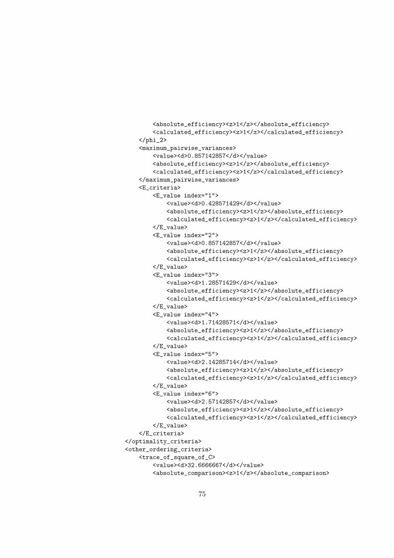
<absolute_efficiency><z>1</z></absolute_efficiency>
<calculated_efficiency><z>1</z></calculated_efficiency>
</phi_2>
<maximum_pairwise_variances>
<value><d>0.857142857</d></value>
<absolute_efficiency><z>1</z></absolute_efficiency>
<calculated_efficiency><z>1</z></calculated_efficiency>
</maximum_pairwise_variances>
<E_criteria>
<E_value index="1">
<value><d>0.428571429</d></value>
<absolute_efficiency><z>1</z></absolute_efficiency>
<calculated_efficiency><z>1</z></calculated_efficiency>
</E_value>
<E_value index="2">
<value><d>0.857142857</d></value>
<absolute_efficiency><z>1</z></absolute_efficiency>
<calculated_efficiency><z>1</z></calculated_efficiency>
</E_value>
<E_value index="3">
<value><d>1.28571429</d></value>
<absolute_efficiency><z>1</z></absolute_efficiency>
<calculated_efficiency><z>1</z></calculated_efficiency>
</E_value>
<E_value index="4">
<value><d>1.71428571</d></value>
<absolute_efficiency><z>1</z></absolute_efficiency>
<calculated_efficiency><z>1</z></calculated_efficiency>
</E_value>
<E_value index="5">
<value><d>2.14285714</d></value>
<absolute_efficiency><z>1</z></absolute_efficiency>
<calculated_efficiency><z>1</z></calculated_efficiency>
</E_value>
<E_value index="6">
<value><d>2.57142857</d></value>
<absolute_efficiency><z>1</z></absolute_efficiency>
<calculated_efficiency><z>1</z></calculated_efficiency>
</E_value>
</E_criteria>
</optimality_criteria>
<other_ordering_criteria>
<trace_of_square_of_C>
<value><d>32.6666667</d></value>
<absolute_comparison><z>1</z></absolute_comparison>
75

<calculated_comparison><z>1</z></calculated_comparison>
</trace_of_square_of_C>
<max_min_ratio_canonical_variances>
<value><d>1.0</d></value>
<absolute_comparison><z>1</z></absolute_comparison>
<calculated_comparison><z>1</z></calculated_comparison>
</max_min_ratio_canonical_variances>
<max_min_ratio_pairwise_variances>
<value><d>1.0</d></value>
<absolute_comparison><z>1</z></absolute_comparison>
<calculated_comparison><z>1</z></calculated_comparison>
</max_min_ratio_pairwise_variances>
<no_distinct_canonical_variances>
<value><z>1</z></value>
<absolute_comparison><z>1</z></absolute_comparison>
<calculated_comparison><z>1</z></calculated_comparison>
</no_distinct_canonical_variances>
<no_distinct_pairwise_variances>
<value><z>1</z></value>
<absolute_comparison><z>1</z></absolute_comparison>
<calculated_comparison><z>1</z></calculated_comparison>
</no_distinct_pairwise_variances>
</other_ordering_criteria>
<canonical_efficiency_factors no_distinct="1" ordered="true">
<value multiplicity="6"><d>0.777777778</d></value>
</canonical_efficiency_factors>
<functions_of_efficiency_factors>
<harmonic_mean alias="A">
<value><d>0.777777778</d></value>
</harmonic_mean>
<geometric_mean alias="D">
<value><d>0.777777778</d></value>
</geometric_mean>
<minimum alias="E">
<value><d>0.777777778</d></value>
</minimum>
</functions_of_efficiency_factors>
</statistical_properties>
</block_design>
<info>
<creator>
<software>
bdstat 0.5/13
</software>
</creator>
76

<creator>
<software>
Design 1.0rev8/51
</software>
</creator>
<reference>
Any book on combinatorial design theory
</reference>
<note>
Fano plane
</note>
<note>
The unique 2-(7,3,1) up to isomorphism
</note>
</info>
</list_of_designs>
77

C GNU Free Documentation License
GNU Free Documentation License
Version 1.2, November 2002
Copyright (C) 2000,2001,2002 Free Software Foundation, Inc.
59 Temple Place, Suite 330, Boston, MA 02111-1307 USA
Everyone is permitted to copy and distribute verbatim copies
of this license document, but changing it is not allowed.
0. PREAMBLE
The purpose of this License is to make a manual, textbook, or other
functional and useful document "free" in the sense of freedom: to
assure everyone the effective freedom to copy and redistribute it,
with or without modifying it, either commercially or noncommercially.
Secondarily, this License preserves for the author and publisher a way
to get credit for their work, while not being considered responsible
for modifications made by others.
This License is a kind of "copyleft", which means that derivative
works of the document must themselves be free in the same sense. It
complements the GNU General Public License, which is a copyleft
license designed for free software.
We have designed this License in order to use it for manuals for free
software, because free software needs free documentation: a free
program should come with manuals providing the same freedoms that the
software does. But this License is not limited to software manuals;
it can be used for any textual work, regardless of subject matter or
whether it is published as a printed book. We recommend this License
principally for works whose purpose is instruction or reference.
1. APPLICABILITY AND DEFINITIONS
This License applies to any manual or other work, in any medium, that
contains a notice placed by the copyright holder saying it can be
distributed under the terms of this License. Such a notice grants a
world-wide, royalty-free license, unlimited in duration, to use that
work under the conditions stated herein. The "Document", below,
refers to any such manual or work. Any member of the public is a
licensee, and is addressed as "you". You accept the license if you
copy, modify or distribute the work in a way requiring permission
under copyright law.
A "Modified Version" of the Document means any work containing the
Document or a portion of it, either copied verbatim, or with
modifications and/or translated into another language.
A "Secondary Section" is a named appendix or a front-matter section of
the Document that deals exclusively with the relationship of the
publishers or authors of the Document to the Document’s overall subject
(or to related matters) and contains nothing that could fall directly
within that overall subject. (Thus, if the Document is in part a
textbook of mathematics, a Secondary Section may not explain any
mathematics.) The relationship could be a matter of historical
connection with the subject or with related matters, or of legal,
commercial, philosophical, ethical or political position regarding
them.
The "Invariant Sections" are certain Secondary Sections whose titles
are designated, as being those of Invariant Sections, in the notice
that says that the Document is released under this License. If a
section does not fit the above definition of Secondary then it is not
allowed to be designated as Invariant. The Document may contain zero
Invariant Sections. If the Document does not identify any Invariant
Sections then there are none.
The "Cover Texts" are certain short passages of text that are listed,
as Front-Cover Texts or Back-Cover Texts, in the notice that says that
the Document is released under this License. A Front-Cover Text may
be at most 5 words, and a Back-Cover Text may be at most 25 words.
78
A "Transparent" copy of the Document means a machine-readable copy,
represented in a format whose specification is available to the
general public, that is suitable for revising the document
straightforwardly with generic text editors or (for images composed of
pixels) generic paint programs or (for drawings) some widely available
drawing editor, and that is suitable for input to text formatters or
for automatic translation to a variety of formats suitable for input
to text formatters. A copy made in an otherwise Transparent file
format whose markup, or absence of markup, has been arranged to thwart
or discourage subsequent modification by readers is not Transparent.
An image format is not Transparent if used for any substantial amount
of text. A copy that is not "Transparent" is called "Opaque".
Examples of suitable formats for Transparent copies include plain
ASCII without markup, Texinfo input format, LaTeX input format, SGML
or XML using a publicly available DTD, and standard-conforming simple
HTML, PostScript or PDF designed for human modification. Examples of
transparent image formats include PNG, XCF and JPG. Opaque formats
include proprietary formats that can be read and edited only by
proprietary word processors, SGML or XML for which the DTD and/or
processing tools are not generally available, and the
machine-generated HTML, PostScript or PDF produced by some word
processors for output purposes only.
The "Title Page" means, for a printed book, the title page itself,
plus such following pages as are needed to hold, legibly, the material
this License requires to appear in the title page. For works in
formats which do not have any title page as such, "Title Page" means
the text near the most prominent appearance of the work’s title,
preceding the beginning of the body of the text.
A section "Entitled XYZ" means a named subunit of the Document whose
title either is precisely XYZ or contains XYZ in parentheses following
text that translates XYZ in another language. (Here XYZ stands for a
specific section name mentioned below, such as "Acknowledgements",
"Dedications", "Endorsements", or "History".) To "Preserve the Title"
of such a section when you modify the Document means that it remains a
section "Entitled XYZ" according to this definition.
The Document may include Warranty Disclaimers next to the notice which
states that this License applies to the Document. These Warranty
Disclaimers are considered to be included by reference in this
License, but only as regards disclaiming warranties: any other
implication that these Warranty Disclaimers may have is void and has
no effect on the meaning of this License.
2. VERBATIM COPYING
You may copy and distribute the Document in any medium, either
commercially or noncommercially, provided that this License, the
copyright notices, and the license notice saying this License applies
to the Document are reproduced in all copies, and that you add no other
conditions whatsoever to those of this License. You may not use
technical measures to obstruct or control the reading or further
copying of the copies you make or distribute. However, you may accept
compensation in exchange for copies. If you distribute a large enough
number of copies you must also follow the conditions in section 3.
You may also lend copies, under the same conditions stated above, and
you may publicly display copies.
3. COPYING IN QUANTITY
If you publish printed copies (or copies in media that commonly have
printed covers) of the Document, numbering more than 100, and the
Document’s license notice requires Cover Texts, you must enclose the
copies in covers that carry, clearly and legibly, all these Cover
Texts: Front-Cover Texts on the front cover, and Back-Cover Texts on
the back cover. Both covers must also clearly and legibly identify
you as the publisher of these copies. The front cover must present
the full title with all words of the title equally prominent and
visible. You may add other material on the covers in addition.
Copying with changes limited to the covers, as long as they preserve
the title of the Document and satisfy these conditions, can be treated
79

as verbatim copying in other respects.
If the required texts for either cover are too voluminous to fit
legibly, you should put the first ones listed (as many as fit
reasonably) on the actual cover, and continue the rest onto adjacent
pages.
If you publish or distribute Opaque copies of the Document numbering
more than 100, you must either include a machine-readable Transparent
copy along with each Opaque copy, or state in or with each Opaque copy
a computer-network location from which the general network-using
public has access to download using public-standard network protocols
a complete Transparent copy of the Document, free of added material.
If you use the latter option, you must take reasonably prudent steps,
when you begin distribution of Opaque copies in quantity, to ensure
that this Transparent copy will remain thus accessible at the stated
location until at least one year after the last time you distribute an
Opaque copy (directly or through your agents or retailers) of that
edition to the public.
It is requested, but not required, that you contact the authors of the
Document well before redistributing any large number of copies, to give
them a chance to provide you with an updated version of the Document.
4. MODIFICATIONS
You may copy and distribute a Modified Version of the Document under
the conditions of sections 2 and 3 above, provided that you release
the Modified Version under precisely this License, with the Modified
Version filling the role of the Document, thus licensing distribution
and modification of the Modified Version to whoever possesses a copy
of it. In addition, you must do these things in the Modified Version:
A. Use in the Title Page (and on the covers, if any) a title distinct
from that of the Document, and from those of previous versions
(which should, if there were any, be listed in the History section
of the Document). You may use the same title as a previous version
if the original publisher of that version gives permission.
B. List on the Title Page, as authors, one or more persons or entities
responsible for authorship of the modifications in the Modified
Version, together with at least five of the principal authors of the
Document (all of its principal authors, if it has fewer than five),
unless they release you from this requirement.
C. State on the Title page the name of the publisher of the
Modified Version, as the publisher.
D. Preserve all the copyright notices of the Document.
E. Add an appropriate copyright notice for your modifications
adjacent to the other copyright notices.
F. Include, immediately after the copyright notices, a license notice
giving the public permission to use the Modified Version under the
terms of this License, in the form shown in the Addendum below.
G. Preserve in that license notice the full lists of Invariant Sections
and required Cover Texts given in the Document’s license notice.
H. Include an unaltered copy of this License.
I. Preserve the section Entitled "History", Preserve its Title, and add
to it an item stating at least the title, year, new authors, and
publisher of the Modified Version as given on the Title Page. If
there is no section Entitled "History" in the Document, create one
stating the title, year, authors, and publisher of the Document as
given on its Title Page, then add an item describing the Modified
Version as stated in the previous sentence.
J. Preserve the network location, if any, given in the Document for
public access to a Transparent copy of the Document, and likewise
the network locations given in the Document for previous versions
it was based on. These may be placed in the "History" section.
You may omit a network location for a work that was published at
least four years before the Document itself, or if the original
publisher of the version it refers to gives permission.
K. For any section Entitled "Acknowledgements" or "Dedications",
Preserve the Title of the section, and preserve in the section all
the substance and tone of each of the contributor acknowledgements
and/or dedications given therein.
L. Preserve all the Invariant Sections of the Document,
unaltered in their text and in their titles. Section numbers
or the equivalent are not considered part of the section titles.
80

M. Delete any section Entitled "Endorsements". Such a section
may not be included in the Modified Version.
N. Do not retitle any existing section to be Entitled "Endorsements"
or to conflict in title with any Invariant Section.
O. Preserve any Warranty Disclaimers.
If the Modified Version includes new front-matter sections or
appendices that qualify as Secondary Sections and contain no material
copied from the Document, you may at your option designate some or all
of these sections as invariant. To do this, add their titles to the
list of Invariant Sections in the Modified Version’s license notice.
These titles must be distinct from any other section titles.
You may add a section Entitled "Endorsements", provided it contains
nothing but endorsements of your Modified Version by various
parties--for example, statements of peer review or that the text has
been approved by an organization as the authoritative definition of a
standard.
You may add a passage of up to five words as a Front-Cover Text, and a
passage of up to 25 words as a Back-Cover Text, to the end of the list
of Cover Texts in the Modified Version. Only one passage of
Front-Cover Text and one of Back-Cover Text may be added by (or
through arrangements made by) any one entity. If the Document already
includes a cover text for the same cover, previously added by you or
by arrangement made by the same entity you are acting on behalf of,
you may not add another; but you may replace the old one, on explicit
permission from the previous publisher that added the old one.
The author(s) and publisher(s) of the Document do not by this License
give permission to use their names for publicity for or to assert or
imply endorsement of any Modified Version.
5. COMBINING DOCUMENTS
You may combine the Document with other documents released under this
License, under the terms defined in section 4 above for modified
versions, provided that you include in the combination all of the
Invariant Sections of all of the original documents, unmodified, and
list them all as Invariant Sections of your combined work in its
license notice, and that you preserve all their Warranty Disclaimers.
The combined work need only contain one copy of this License, and
multiple identical Invariant Sections may be replaced with a single
copy. If there are multiple Invariant Sections with the same name but
different contents, make the title of each such section unique by
adding at the end of it, in parentheses, the name of the original
author or publisher of that section if known, or else a unique number.
Make the same adjustment to the section titles in the list of
Invariant Sections in the license notice of the combined work.
In the combination, you must combine any sections Entitled "History"
in the various original documents, forming one section Entitled
"History"; likewise combine any sections Entitled "Acknowledgements",
and any sections Entitled "Dedications". You must delete all sections
Entitled "Endorsements".
6. COLLECTIONS OF DOCUMENTS
You may make a collection consisting of the Document and other documents
released under this License, and replace the individual copies of this
License in the various documents with a single copy that is included in
the collection, provided that you follow the rules of this License for
verbatim copying of each of the documents in all other respects.
You may extract a single document from such a collection, and distribute
it individually under this License, provided you insert a copy of this
License into the extracted document, and follow this License in all
other respects regarding verbatim copying of that document.
7. AGGREGATION WITH INDEPENDENT WORKS
A compilation of the Document or its derivatives with other separate
81
and independent documents or works, in or on a volume of a storage or
distribution medium, is called an "aggregate" if the copyright
resulting from the compilation is not used to limit the legal rights
of the compilation’s users beyond what the individual works permit.
When the Document is included in an aggregate, this License does not
apply to the other works in the aggregate which are not themselves
derivative works of the Document.
If the Cover Text requirement of section 3 is applicable to these
copies of the Document, then if the Document is less than one half of
the entire aggregate, the Document’s Cover Texts may be placed on
covers that bracket the Document within the aggregate, or the
electronic equivalent of covers if the Document is in electronic form.
Otherwise they must appear on printed covers that bracket the whole
aggregate.
8. TRANSLATION
Translation is considered a kind of modification, so you may
distribute translations of the Document under the terms of section 4.
Replacing Invariant Sections with translations requires special
permission from their copyright holders, but you may include
translations of some or all Invariant Sections in addition to the
original versions of these Invariant Sections. You may include a
translation of this License, and all the license notices in the
Document, and any Warranty Disclaimers, provided that you also include
the original English version of this License and the original versions
of those notices and disclaimers. In case of a disagreement between
the translation and the original version of this License or a notice
or disclaimer, the original version will prevail.
If a section in the Document is Entitled "Acknowledgements",
"Dedications", or "History", the requirement (section 4) to Preserve
its Title (section 1) will typically require changing the actual
title.
9. TERMINATION
You may not copy, modify, sublicense, or distribute the Document except
as expressly provided for under this License. Any other attempt to
copy, modify, sublicense or distribute the Document is void, and will
automatically terminate your rights under this License. However,
parties who have received copies, or rights, from you under this
License will not have their licenses terminated so long as such
parties remain in full compliance.
10. FUTURE REVISIONS OF THIS LICENSE
The Free Software Foundation may publish new, revised versions
of the GNU Free Documentation License from time to time. Such new
versions will be similar in spirit to the present version, but may
differ in detail to address new problems or concerns. See
http://www.gnu.org/copyleft/.
Each version of the License is given a distinguishing version number.
If the Document specifies that a particular numbered version of this
License "or any later version" applies to it, you have the option of
following the terms and conditions either of that specified version or
of any later version that has been published (not as a draft) by the
Free Software Foundation. If the Document does not specify a version
number of this License, you may choose any version ever published (not
as a draft) by the Free Software Foundation.
82