The Expanding Empire and Spatial Distribution of Economic … · · 2016-02-15impact of the...

CIRJE Discussion Papers can be downloaded without charge from:

http://www.cirje.e.u-tokyo.ac.jp/research/03research02dp.html

Discussion Papers are a series of manuscripts in their draft form. They are not intended for

circulation or distribution except as indicated by the author. For that reason Discussion Papers

may not be reproduced or distributed without the written consent of the author.

CIRJE-F-968

The Expanding Empire and Spatial Distribution of Economic Activities: The Case of the Colonization

of Korea by Japan in the Prewar Period

Kentaro Nakajima Tohoku University

Tetsuji Okazaki The University of Tokyo

March 2015; Revised in July 2015

The Expanding Empire and Spatial Distribution of Economic Activities:

The Case of the Colonization of Korea by Japan in the Prewar Period

July 2015

Kentaro Nakajima (Tohoku University)*

and

Tetsuji Okazaki (University of Tokyo)**

Abstract

After the First Sino-Japanese War and the Russo-Japanese War, Japan annexed Korea

in 1910. We exploit this event as a natural experiment to investigate the effect of

improved market accessibility on population growth. It is found that the drastic tariff

reduction caused by the annexation raised the population growth rates and that the

impact of the tariff reduction was significantly larger in areas close to the eliminated

border between Japan and Korea. As predicted by spatial economics theory, market

accessibility was indeed a determinant of the spatial distribution of economic activities.

In the context of economic history, our findings suggest that it is important to

reconsider the economic consequences of imperialism from the angle of spatial

economics.

JEL classification: N45, N95, R12

Key words: Imperialism, Colonization, Spatial economics, Economic geography,

Economic History,

Japan

* [email protected] ** [email protected]

I

The rise and fall of the Empire of Japan was one of the most remarkable events

in the twentieth century history of imperialism. Japan annexed Taiwan, southern

Sakhalin and Korea around the turn of the century during the Sino-Japanese War and

the Russo-Japanese War. The Empire of Japan expanded its control over the northern

part of China and Southeast Asia in the 1930s and 1940s and then suddenly lost the

acquired territories following its defeat in WWII.1 The military and political integration

of these large areas into the Empire of Japan had a substantial impact on the economy

of Japan itself as well as on the integrated areas. This paper explored how the

annexation of Korea affected the Japanese economy.

In particular, we focus on the effect that annexation had on the spatial

distribution of economic activities in Japan. Market accessibility has long been

considered to be one of the basic determinants of the spatial distribution of economic

activities in the theoretical literature of spatial economics.2 More specifically, market

accessibility has been presumed to have a positive effect on economic activities.

Redding and Sturm estimated the role of market accessibility on the spatial

distributions of economic activities by focusing on the division of Germany into West

Germany and East Germany just after WWII. 3 As Germany’s division was

implemented for military and political reasons, this event can be regarded as exogenous

to the economy. They interpreted the division as a loss of access to the East German

market for West Germany and tested the theoretical prediction that the impact of the

division would be larger in areas closer to the new border between West Germany and

East Germany. They found that the German division indeed had a negative impact on

population growth in the cities close to the new border. In the same vein, some papers

examined the implications of market accessibility by focusing on the division of an

economy or the integration of economies.4

In this context, the rise and fall of the Empire of Japan is an important subject to

explore. Nakajima focused on the independence of Korea from Japan in 1945 to

examine the implications of market accessibility, finding that cities in the western part

of Japan close to the new border between Japan and Korea suffered from a greater

negative impact from the division,5 which is consistent with Redding and Sturm’ s

1 On the economy of the Empire of Japan in the 1930s and 1940s, see Bordorf and Okazaki eds., Economies under Occupation; Hara, Nihon Senji Keizai Kenkyu; Yamamoto, Nihon Shokuminchi Keizaishi Kenkyu. 2 E.g., Fujita et al., Spatial Economics. 3 Redding and Strum, ‘The cost of remoteness.’ 4 Brülhart et al., ‘How Wages and Employment Adjust to Trade Liberalization’; Ahlheldt et al., ‘The Economics of Density’; Nakajima, ‘Economic Division and Spatial Relocation.’ 5 Nakajima, ‘Economic Division and Spatial Relocation.’

results.6

This paper also focuses on the border change between Japan and Korea, but the

direction of the change here is opposite to Nakajima.7 Namely, we exploit the event of

Japan’s annexation of Korea in 1910 as a natural experiment. Similar to the division

and the unification of Germany after World War II, the annexation of Korea can be

regarded as a natural experiment exogenous to economic variables because its cause

was principally military and political.8 After the annexation, the Japanese government

and the colonial government, i.e., the Governor-General of Korea, sequentially reduced

the tariff barrier between Japan and Korea to integrate Korea into the Japanese trade

area. This event provides a good opportunity to investigate the implications of market

accessibility. In line with the literature, the annexation of Korea would improve

accessibility to the Korean market from Japan and thereby affect the spatial

distribution of economic activities in Japan. More specifically, the areas closer to the

previous border between Japan and Korea would enjoy a larger positive impact from

the integration.

By using regional population data, we estimate the tariff reduction effects by

using a difference-in-differences (DD) design similar to Redding and Sturm (2008),

finding the following results. First, regions close to Korea experienced a 6% increase in

population relative to the other regions over the 15 years following the integration. This

implies the increased market accessibility by the annexation of Korea positively affects

the regional economy close to Korea. Second, integration effects are only observed in

villages; non-villages such as cities and towns are not affected by the integration in

terms of population. This means that the annexation of Korea positively affects only

smaller regions. Finally, we examined the difference in the impact across industries.

This enabled us to confirm the channel through which the border removal affected the

spatial distribution of economic activities. Within the regions close to Korea, those

regions specialized in industries that export to Korea gained more. These results

support the notion that the annexation of Korea increased the accessibility of the

Japanese industries to the Korean market especially in those regions close to Korea,

and the increased market accessibility contributed to regional development. In

particular, the result showing that regions enjoying a stronger economic relationship to

the Korean market benefitted more than the other regions strongly supports our story.

In the context of the economic history of the Empire of Japan, it is known that

after the annexation, the Korean economy was integrated into the economy of the 6 Redding and Strum, ‘The cost of remoteness.’ 7 Nakajima, ‘Economic Division and Spatial Relocation.’ 8 Unno, Kankoku Heigo.

Empire as a supplier of agrarian products, especially rice, and as a market for Japanese

industrial products, including cotton textiles.9 This paper will contribute to this strand

of literature by introducing the perspective of spatial economics and exploring the

impact of the annexation on the spatial distribution of economic activities within Japan

proper.

The remainder of the paper is organized as follows. Section II describes the brief

history of the integration of Korea into Japan. Section III explains the theoretical

framework, data, and estimation strategy. In Section IV, we present the estimation

results. Section V concludes the paper.

II

Just after the Meiji Restoration, some influential politicians in Japan conceived

of integrating Korea under Japan’s influence. However, two great powers in the Far

East, China and Russia, also had keen interest in Korea. Indeed, Korea was an area of

focus for political and military conflicts in this area in the late nineteenth and early

twentieth centuries. Given this situation, Japan first excluded the influence of China

from Korea through the Sino-Japanese War I (1894-95). Korea had been a tributary

country of China since the ancient period, but China recognized the independence of

Korea by the Shimonoseki Peace Treaty in 1895. After that, and especially after the

Boxer Uprising in Northern China in 1901, the threat of Russia to Korea increased; this

resulted in the Russo-Japanese War (1904-05), through which Japan established its

dominant position in Korea. Based on the situation, in 1905, Japan made Korea a

protectorate, supervised by a Resident-General (Tokan) appointed by the Japanese

government. Finally in 1910, Japan formally annexed Korea and established a

Governor-General (Sotoku-fu) there. In other words, Korea became a colony of the

Empire of Japan, in addition to Taiwan and the southern part of Sakhalin.10

The principle of the Japanese government in colonizing Korea was “assimilation,”

that is, introducing Japanese institutions into Korea. In accordance with this principle,

the Japanese government aimed to integrate Korea into its trade area. The same tariff

rates were to be applied to the commodities imported from foreign countries to Japan

and Korea, while all the tariffs should be removed within this trade area in the Empire

of Japan.11

Before the annexation, the Korean government had agreements on tariff rates

9 Yamamoto, Nihon Shokuminchi Keizaishi Kenkyu; Hori, Higashi Asia Shihonshugishi-ron. 10 Unno, Kankoku Heigo. 11 Kim, Nihon Teikokushugi kano Chosen Keizai, pp.20-24; Yamamoto, Nihon Shokuminchi Keizaishi Kenkyu, pp.3-62.

with several countries, including Russia, the U.K. and the U.S., based on partial trade

treaties. To mitigate the antipathies of those countries to the annexation of Korea, in

August 1910, the Japanese government declared that Korea’s tariff system would be

deferred for the next ten years, until August 1920. It should be noted that the tariffs

between Japan and Korea were included in this declaration as well.12

However, the Japanese government implemented several amendments to the

Korean tariff system before 1920. The most important change was the removal in 1913

of the tariffs on rice and unhulled rice imported from Korea to Japan.13 Because rice

was the largest commodity that Japan imported from Korea, the impact of this change

was substantial. Data on the amount of commodities imported from Korea to Japan, as

well as on the amount of tariffs imposed on them, are available in the Annual Return of

the Foreign Trade of the Empire of Japan (Dainihon Gaikoku Boeki Nenpyo). Dividing

the tariff revenue by import amount, we have the average tariff rate. Figure 1 indicates

the average tariff rate on the commodities imported from Korea as well as the import

amount. The impact of rice tariff removal is clearly reflected in this figure. The average

tariff rate declined from 10.7% in 1912 to 3.6% in 1914, while the import increased by

1.9 times in this period.

Figure 1

In September 1920, when the declaration on the deferment of the tariff system

expired, the Japanese government removed all of the tariffs on the commodities

imported from Korea. However, the tariffs on the commodities imported from Japan to

Korea were not removed at that time, although the declaration had expired. This was

because the Governor-General of Korea depended heavily on import tariff revenue

generated by commodities from Japan. 14 However, this unbalanced tariff policy

received criticism from the Japanese Diet, and as a result, in April 1923, all tariffs on

commodities that Korea imported from Japan were removed with the exception of

three items – alcohol, alcoholic beverages and fabrics.15 The proportion of these three

items in Korean imports from Japan was not negligible, but the impact of this reform

was substantial. Figure 2 indicates the average tariff rate on commodities imported

from Japan to Korea. As we can see in this figure, the average tariff rate declined from

12 Kim, Nihon Teikokushugi kano Chosen Keizai, p30; Yamamoto, Nihon Shokuminchi Keizaishi Kenkyu, p.69. 13 Yamamoto, Nihon Shokuminchi Keizaishi Kenkyu, p.70. 14 Ibid., pp.70-71. 15 Ibid., p.72.

5.68% in 1922 to 1.32% in 1924. Furthermore, the import tariff rate on fabrics from

Japan decreased from 7.5% to 5% in April 1927. As shown in Figure 1 and Figure 2, the

integration of Korea into the Japanese trade area, which had been intended by the

Japanese government since the annexation, was largely achieved by 1924. Table 1

summarizes the composition of trade between Japan and Korea by commodity group.

Major items of import to Korea from Japan were textiles as well as chemicals, metals

and machinery, while agricultural products, particularly rice, formed the largest import

to Japan from Korea.

Figure 2, Table 1

III

Theoretical background

For the theoretical framework, we follow Redding and Sturm's model,16 which

builds on Helpman.17 In this section, we briefly present their model. Their model

comprises 1, … regions, two goods (manufacturing and housing), and two inputs

(labor and land). The manufacturing sector needs only labor as an input for production,

with increasing returns to scale technology. The housing sector has constant returns to

scale technology with an inelastic land input ( ) supplied.

A representative consumer living in region has a Cobb-Douglas preference on

consumption for manufacturing goods and housing services , with a share of

manufacturing goods . The sub-utility for manufacturing goods is of the constant

elasticity of substitution (CES) form, with the elasticity of substitution among varieties

( ).

While housing services are not tradable, manufacturing goods are tradable among

regions with iceberg transport costs. If one unit of the manufacturing good is shipped

from region to region , only fraction 1/ of the original unit actually arrives.

In this model, two indices of accessibility determine the characteristics of the

equilibrium. Market access in region ( ∑ ) represents

the accessibility to the demand market, where is the manufacturing wage, is the

population, and is the price index in region . Market access is the transport

cost-weighted sum of the demands for manufacturing goods in each region, adjusted by

16 Redding and Strum, ‘The cost of remoteness.’ 17 Helpman, ‘The size of regions.’

competition effect . Supplier access ( ∑ ) represents the

accessibility to the sources of supply, where is the number of manufacturing

varieties produced in city , and is the corresponding price. Supplier access is the

transport cost-weighted sum of supplies for manufacturing goods in region .

Under this setup, in a long-run equilibrium, the population of labor in region is

an increasing function of market access:

where is the composite of parameters. The transport cost is assumed to be an

increasing function of distance. Therefore, the integration of two markets increases

market access in regions near the border, and its effect diminishes according to the

distance from the border.

The integration of two markets would increase the market access of regions close

to the border, leading to a relative increase in the real wages in these regions. This

would be accompanied by labor inflows into the concerned regions. However, such

labor inflows would increase the housing rent, which would decrease the real wages in

those cities, resulting in the real wages being equalized across all regions in the

long-run equilibrium.

Data and empirical strategy

We use panel data on the population of 3,851 Japanese municipalities (city, town,

and village) for the years 1913, 1920, 1925, and 1935; these data are obtained from the

Bureau of Statistics, Imperial Cabinet. 18 The distance between municipalities is

measured by the great circle distance between centroids of municipalities obtained by

historical GIS (Geographical Information Science) data.19

Using these data, we empirically investigate the hypothesis derived from the

theoretical model above, which states that regions located close to the border show a

relative increase in their population growth rates compared to the regions situated

further from the border. We divide the Japanese regions into two groups: border

regions (treatment group) and non-border regions (control group). The Japanese

regions located close to Korea are classified as border regions, while the others are

non-border regions. Following Nakajima,20 we define the border regions as those

18 Bureau of Statistics, Imperial Cabinet, Nihon Teikoku Jinko Seitai Tokei; Bureau of Statistics, Imperial Cabinet, Showa10-nen Kokusei Chosa Hokoku. 19 Murayama Laboratory in Tsukuba University. 20 Nakajima, ‘Economic Division and Spatial Relocation.’

located within 400 km of Pusan, which is the Korean city closest to Japan and has the

busiest port in terms of trade between Japan and Korea. The boundary for the border

region group is encircled in Figure 3. Pusan is located at the center of a circle that

defines a distance of 400 km as its radius. The number of regions included as border

regions is 542, while the remainder (3,309 regions) fall under the category of

non-border regions.

We also divide the periods into before and after the treatment. As we see in

Section 2, tariff removal occurred in 1920 and 1923. Thus, we consider the periods 1913

and 1920 as before-treatment periods, and periods 1925 and 1935 as after-treatment

periods.

Figure 3

We econometrically compare the population growth rates of these two groups by

using the DD methodology. The estimation equation is as follows:

where is the population growth rate in region in period ; is

the border region dummy, which is one if city is a border region; 1 if

1920; and is the year dummy to control for common macroeconomic shocks.

Our primary interest is parameter , which captures the treatment effect of

integration on the population growth rate of the border regions compared to that of the

non-border regions. The result that is significantly positive indicates a greater

increase in the growth rate of the border regions than in that of the non-border regions

due to the integration of the Korean market; this is consistent with the theoretical

prediction.

IV

Baseline results

Column (1) in Table 2 shows the baseline results. Our primary interest is the

coefficient of Border Integration, which is positive and significant. This is consistent

with the theoretical prediction. Additionally, the magnitude of the coefficient was large.

Border regions have 0.4 percentage points of annual population growth rate after

integration. This implies that after the integration, the border regions experience a 6%

increase in population relative to the other regions over the 15 years following the

integration.

Another important consequence of the theoretical model is that small regions

experience a greater integration effect than that experienced by large regions.

Intuitively, this is because own markets are relatively less important for small regions

than the own markets are for large regions. In other words, the economy of a small

region depends more on the markets in other regions than the economy of a large

region does; hence, the impact of the improved access to the Korean market was

expected to be greater for small regions than for large regions.

To examine this prediction, Column (2) restricts the samples to the non-village

regions that include cities and towns, which are supposed to be large regions. In this

specification, the coefficient of Border Integration is positive but not statistically

significant. That is, there is no statistically significant integration effect for the

non-village regions. Column (3) restricts samples to the villages, which are supposed to

be small regions. In this specification, the coefficient of Border Integration is positive

and statistically significant. These results suggest that economic integration affected

the population growth rate especially for villages or small regions. This is consistent

with the theoretical prediction.21

Table 2

Because the driving force behind the annexation of Korea was political and

military, similar to the division and unification of Germany, it can be assumed that

economic integration and hence the determination of border cities was not correlated

with economic factors. However, one may be concerned that heterogeneity existed

between the border and non-border regions. For example, initial levels of

industrialization would affect population growth after integration. To control for such

heterogeneity, we use a matching technique. We choose samples of the non-border

regions that are as similar as possible to the border regions in terms of their initial

conditions. We match populations in 1913 and 1920 by minimizing the difference

between the border and non-border regions. Thus, we can compare the border and

non-border cities that had similar initial populations and population growth rates. The

results are shown in Table 3. Column (1) shows the baseline, Column (2) shows the

non-village, and Column (3) shows the village results. Even if we match samples, we 21 Recently, Brülhart, Carrère, and Robert-Nicoud, ‘Trade and Towns,’ proposed a theoretical model that can explain the heterogeneous treatment effects between large and small regions and confirm their prediction. They find that large cities do not increase their employment after integration because the accompanying large increase in the nominal wage cancels the effects for employment. Our results are also consistent with their theoretical prediction.

obtain very similar results. The integration effects are robustly observed, especially in

villages.

Table 3

Furthermore, our theoretical model implies that the treatment effects differ

across locations. To observe such heterogeneity in the treatment effect, we first

estimate the heterogeneous treatment effect by a series of dummies for cities lying

within cells 50 km wide at varying distances from Pusan, ranging from 250 to 500 km.

We include these series of dummies and the interaction terms on the integration

dummy in the estimation equation. The results are shown in Table 4. The coefficients of

the interaction terms for 0-250 km, 250-300 km, and 300-350 km are positive and

significant at the 5% level. However, the coefficients of the interaction term for over

350 km are not significant. These results support our theoretical hypothesis.

Table 4

Furthermore, we test the heterogeneity on the treatment effects by the individual

treatment effect using the estimation equation given below:

where is the number of regions and is the region fixed effect. The parameter

captures the mean population growth in region j before the integration, while

captures the individual treatment effect of economic integration. Figure 4 graphs the

estimated individual treatment effect ( ) against the distance from Pusan.22 We

normalize the treatment effect such that the mean value is zero. The green solid line

represents the results of fractional polynomials, and the dark region represents its 95%

confidence intervals. The results of the fractional polynomials have a peak in the region

nearest to Pusan, then gradually decline with distance. These results support the

theoretical implications that the integration of two markets increases populations in

regions near the border, and its effect diminishes according to the distance from the

border.

22 To reduce the sample size to estimate fixed effect in each region, we randomly choose 30% of total observations.

Figure 4

Exporting industry

In the previous section, we find a significant positive increase in population in

regions close to Korea after integration. If the population growth in border regions after

the annexation of Korea is actually caused by the market access improvement predicted

by theory, regions that have stronger economic relationships with Korea will gain more

than the other regions from integration. In this subsection, we focus on an industry

exporting from Japan to Korea as a measure of the economic relationship.

As we saw in Section 2, the largest commodity that Japan exported to Korea is

textiles. Thus, the regions specializing in the textile industry have a stronger

relationship with the Korean market and would be more affected by the increase in

market access to Korea than non-specialized regions would be.

We test this hypothesis using the triple difference estimation as follows,

where is a textile dummy that is equal to one if region is specialized in the

textile industry, and zero otherwise. We define the region specialized in the textile

industry by the share of textile plants in the region. For this purpose, we use the micro

data of the Census of Manufactures for 1919 (the eve of the treatment periods). That is,

we obtain the number of plants by industry and region (city, town and village) from the

Ministry of Agriculture and Commerce ed. and calculate the share of textile plants in

each region.23 If the share of textile plants in a region is above the 75th percentile, we

regard it as a textile-specialized region; otherwise, we regard it as a non-specialized

region. The covariates in are all remaining interaction terms and single terms,

, , , , and

. The coefficient captures the triple difference treatment effects. That is, a

positive implies that border regions specialized in the textile industry have a higher

growth rate than the non-textile specialized border regions.

The results are shown in Table 5. Column (1) shows the baseline result. The

coefficient for is positively significant. This is consistent with

the previous analysis. Border regions increase in population after integration. In

addition, the coefficient for is also positively significant. This

implies that regions specializing in textiles gain more in population than the other

regions because of the integration. Furthermore, the coefficient for the triple

interaction, , is also significantly positive. That is, within the border regions where

23 Ministry of Agriculture and Commerce ed., Kojo Tsuran.

there is an increase in population after integration, regions specialized in the textile

industry gain significantly more than other regions from the integration. In other words,

within the regions specializing in textiles where there is an increase in population after

integration, regions close to Korea significantly gain more by the integration than the

other regions. This result strongly supports our story that tariff reduction improves

market access in the regions close to Korea, which increases the population size of the

regions. Column (2) shows the results after matching, which are similar. Our results are

robust for the choice of control group. Column (3) shows the results with restricting the

sample to the non-village regions. Similar to the results in the previous section, the

coefficient for is not significant. However, the triple

difference estimator is positively significant. On average, non-village regions close to

Korea experience no gains from integration, but non-village regions specializing in

textiles experience gains from integration. Finally, Column (4) shows the results with

the sample restricted to villages. The results are similar to the baseline one.

Table 5

V

In 1910, Japan annexed Korea to integrate it into the Empire of Japan. According

to its policy of assimilating colonies, the Japanese government intended to remove

tariffs between Japan and Korea, and this policy was nearly realized by 1923, when

tariffs on the commodities imported from Japan to Korea were essentially removed.

Reduction of the tariff barrier was supposed to improve market access between Japan

and Korea.

We exploit this event as a natural experiment to investigate the effect of improved

market accessibility on population growth. It is found that the tariff reduction raised

the population growth rates and that it occurred only in areas close to the removed

border between Japan and Korea. Furthermore, within the regions close to Korea,

those regions specialized in the textile industry, whose products were the major export

goods to Korea from Japan, gained more than the other regions after the integration.

Our results suggest that market accessibility was indeed a determinant of the

spatial distribution of economic activities as predicted by spatial economics theory. In

the context of economic history, our findings suggest that it is important to reconsider

the economic consequence of imperialism from the angle of spatial economics.

References

[1] Ahlfeldt, M. Gabriel, Stephen J. Redding, Daniel M. Sturm, and Nikolaus Wolf

(2015) The Economics of Density: Evidence from the Berlin Wall, Econometrica,

forthcoming.

[2] Bordorf, Marcel and Tetsuji Okazaki eds. (2015) Economies under Occupation :

The Hegemony of Nazi Germany and Imperial Japan in World War II, London:

Routledge.

[3] Brülhart, Marius, Céline Carrère, and Frédéric Robert-Nicoud (2015) Trade and

Towns: Heterogeneous Adjustment to a Border Shock, mimeo.

[4] Brülhart, Marius, Céline Carrère, and Federico Trionfetti (2012) How Wages and

Employment Adjust to Trade Liberalization: Quasi-Exprimental Evidence from

Austria, Journal of International Economics 86(1), pp. 68 -81.

[5] Bureau of Statistics, Imperial Cabinet (1916) Nihon Teikoku Jinko Seitai Tokei

(State of the Population in the Japan Empire), Tokyo: Bureau of Statistics,

Imperial Cabinet.

[6] Bureau of Statistics, Imperial Cabinet (1936) Showa10-nen Kokusei Chosa

Hokoku, (Report on Population Census for 1935) vol.3, Tokyo: Bureau of Statistics,

Imperial Cabinet.

[7] Fujita, Masahisa, Paul Krugman, and Anthony Venables (1999) The Spatial

Economy: Cities, Regions and International Trade, Cambridge, MIT Press.

[8] Governor-General of Korea (1937) Chosen Boeki Nenpyo (Chosen Table of Trade

and Shipping), 1935 issue, Seoul: Governor-General of Korea

[9] Hara, Akira (2013) Nihon Senji Keizai Kenkyu (A Study on the Japanese War

Economy), Tokyo: The University of Tokyo Press.

[10] Helpman, Elhanan (1998) The size of regions. In: Pines, D., Sadka, E., Zilcha, I.

(Eds.), Topics in Public Economics. Cambridge University Press, Cambridge.

[11] Hori, Kazuo (2009) Higashi Asia Shihonshugishi-ron: Keisei, Kozo, Tenkai (On

the History of the East Asian Capitalism: Formation, Structure and

Development), vol.1, Kyoto: Mineruva Shobo

[12] Kim, Nak Nyeon (2002) Nihon Teikokushugi kano Chosen Keizai (Korean

Economy under the Japan Empire), Tokyo: The University of Tokyo Press

[13] Ministry of Agriculture and Commerce (1921) Kojo Tsuran (Directory of

Factories), Tokyo: The Industry Vlub of Japan

[14] Nakajima, Kentaro (2008) Economic Division and Spatial Relocation: The Case of

Postwar Japan, Journal of the Japanese and International Economies, 22(3), pp.

383-400.

[15] Redding, J. Stephen and Daniel M. Sturm (2008) The Cost of Remoteness:

Evidence from German Division and Reunification, American Economic Review

98(5), pp. 1766-1797.

[16] Unno, Fukuju (1995) Kankoku Heigo (Annexation of Korea), Iwanami Shoten

[17] Yamazawa, Ippei and Yuzo Yamamoto (1979), Boeki to Kokuzai Shushi (Foreign

Trade and Balance of Payments), Tokyo: Toyo Keizai Shinposha

[18] Yamamoto, Yuzo (1992) Nihon Shokuminchi Keizaishi Kenkyu (Research in the

Economic History of the Colonies of Japan), Nagoya: The University of Nagoya

Press.

Figure 1 Percentage of exports to Korea in total Japanese exports and average rate of

tariffs on imports from the Empire of Japan

Source: Yamazawa and Yamamoto (1979), pp.206-209; Governor-General of Korea

(1937), p.7, p.799.

Note: The average tariff rate is the ratio of the tariff revenue of Korea to its total

imports.

0.0

2.0

4.0

6.0

8.0

10.0

12.0

14.0

16.0

18.0

1885 1890 1895 1900 1905 1910 1915 1920 1925 1930 1935

Percentage of export toKorea in the totalexport of Japan

Average tariff rate onimport from JapanEmpire

%

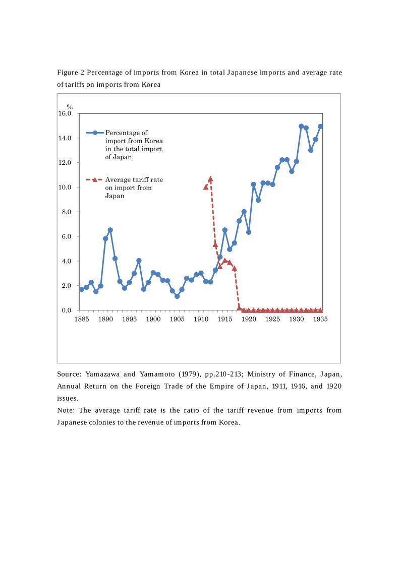
Figure 2 Percentage of imports from Korea in total Japanese imports and average rate

of tariffs on imports from Korea

Source: Yamazawa and Yamamoto (1979), pp.210-213; Ministry of Finance, Japan,

Annual Return on the Foreign Trade of the Empire of Japan, 1911, 1916, and 1920

issues.

Note: The average tariff rate is the ratio of the tariff revenue from imports from

Japanese colonies to the revenue of imports from Korea.

0.0

2.0

4.0

6.0

8.0

10.0

12.0

14.0

16.0

1885 1890 1895 1900 1905 1910 1915 1920 1925 1930 1935

Percentage ofimport from Koreain the total importof Japan

Average tariff rateon import fromJapan

%

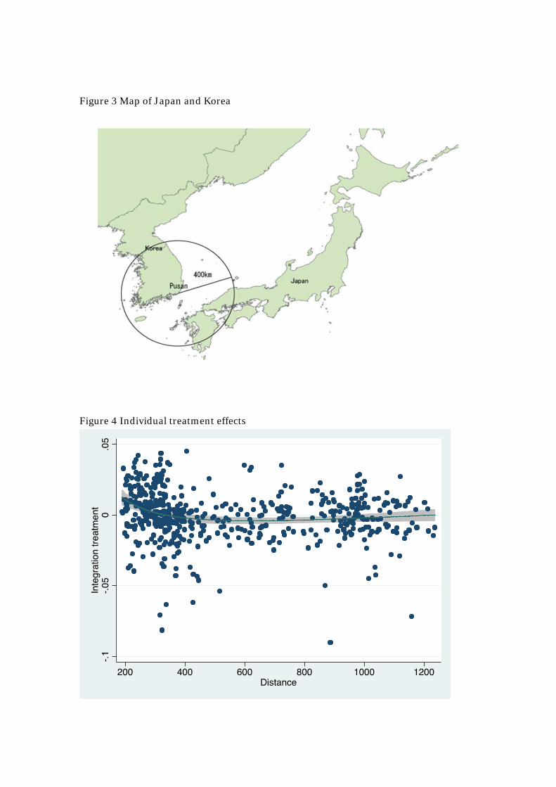
Figure 3 Map of Japan and Korea

Figure 4 Individual treatment effects

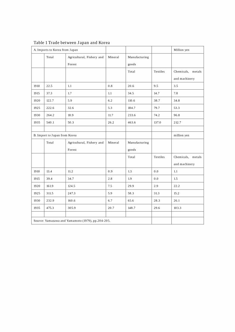
Table 1 Trade between Japan and Korea

A. Imports to Korea from Japan Million yen

Total Agricultural, Fishery and

Forest

Mineral Manufacturing

goods

Total Textiles Chemicals, metals

and machinery

1910 22.5 1.1 0.8 20.6 9.5 3.5

1915 37.3 1.7 1.1 34.5 14.7 7.8

1920 122.7 5.9 6.2 110.6 38.7 34.8

1925 222.6 32.6 5.3 184.7 79.7 53.3

1930 264.2 18.9 11.7 233.6 74.2 96.8

1935 540.1 50.3 26.2 463.6 137.0 212.7

B. Import to Japan from Korea million yen

Total Agricultural, Fishery and

Forest

Mineral Manufacturing

goods

Total Textiles Chemicals, metals

and machinery

1910 13.4 11.2 0.9 1.3 0.0 1.1

1915 39.4 34.7 2.8 1.9 0.0 1.5

1920 161.9 124.5 7.5 29.9 2.9 22.2

1925 311.5 247.3 5.9 58.3 31.3 15.2

1930 232.9 160.6 6.7 65.6 28.3 26.1

1935 475.3 305.9 20.7 148.7 29.6 103.3

Source: Yamazawa and Yamamoto (1979), pp.204-205.

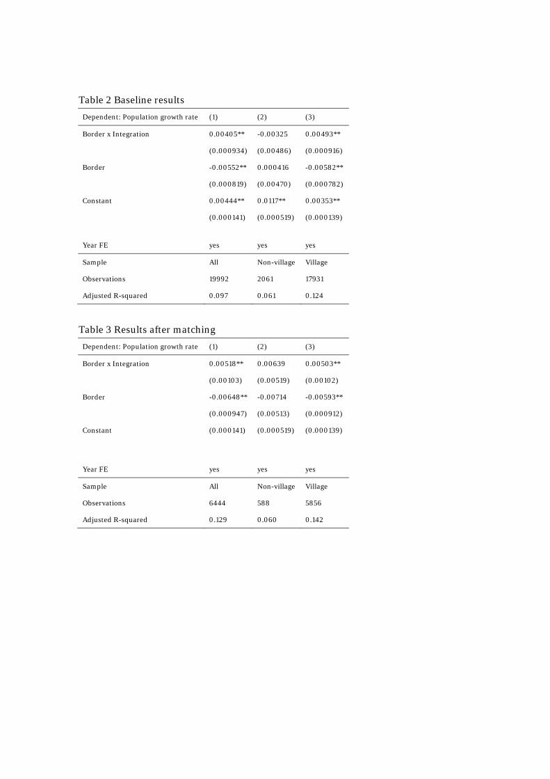
Table 2 Baseline results

Dependent: Population growth rate (1) (2) (3)

Border x Integration 0.00405** -0.00325 0.00493**

(0.000934) (0.00486) (0.000916)

Border -0.00552** 0.000416 -0.00582**

(0.000819) (0.00470) (0.000782)

Constant 0.00444** 0.0117** 0.00353**

(0.000141) (0.000519) (0.000139)

Year FE yes yes yes

Sample All Non-village Village

Observations 19992 2061 17931

Adjusted R-squared 0.097 0.061 0.124

Table 3 Results after matching


Border x Integration 0.00518** 0.00639 0.00503**

(0.00103) (0.00519) (0.00102)

Border -0.00648** -0.00714 -0.00593**

(0.000947) (0.00513) (0.000912)

Constant (0.000141) (0.000519) (0.000139)

Year FE yes yes yes




Table 4 Results on distance cells


Border 0-250 km × Integration 0.00692** -0.0000750 0.00772**

(0.00172) (0.00638) (0.00179)

Border 250-300 km × Integration 0.00447** 0.00482 0.00482**

(0.00124) (0.00468) (0.00128)

Border 300-350 km × Integration 0.00437** 0.00371 0.00471**

(0.00115) (0.00437) (0.00120)

Border 350-400 km × Integration -0.00165 -0.00613 -0.00103

(0.00129) (0.00494) (0.00133)

Border 400-450 km × Integration -0.00163 -0.00909 -0.000681

(0.00186) (0.00668) (0.00193)

Border 450-500 km × Integration 0.00317 0.0175** 0.00137

(0.00211) (0.00474) (0.00212)

Border 0-250 km -0.00705** 0.000168 -0.00737**

(0.00142) (0.00564) (0.00146)

Border 250-300 km -0.00671** -0.00649** -0.00649**

(0.00103) (0.00325) (0.00108)

Border 300-350 km -0.00660** -0.00374 -0.00662**

(0.00107) (0.00417) (0.00111)

Border 350-400 km -0.0000541 0.00470 0.0000387

(0.00129) (0.00391) (0.00134)

Border 400-450 km -0.00104 0.00230 -0.00132

(0.00187) (0.00722) (0.00191)

Border 450-500 km -0.00626** -0.0244** -0.00389**

(0.00191) (0.00590) (0.00189)

Integration 0.0115** 0.0177** 0.0107**

(0.000555) (0.00137) (0.000600)

Constant -0.00780** -0.00496** -0.00820**

(0.000509) (0.00143) (0.000545)

Year FE yes yes yes




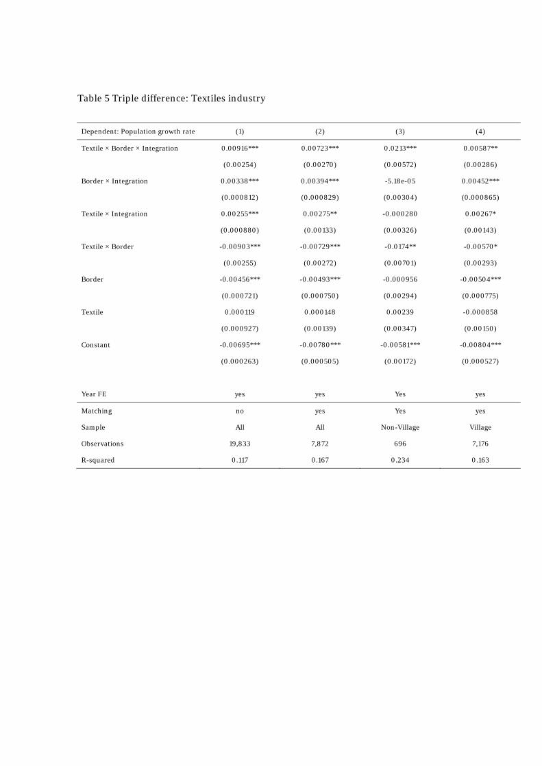
Table 5 Triple difference: Textiles industry

Dependent: Population growth rate (1) (2) (3) (4)

Textile × Border × Integration 0.00916*** 0.00723*** 0.0213*** 0.00587**

(0.00254) (0.00270) (0.00572) (0.00286)

Border × Integration 0.00338*** 0.00394*** -5.18e-05 0.00452***

(0.000812) (0.000829) (0.00304) (0.000865)

Textile × Integration 0.00255*** 0.00275** -0.000280 0.00267*

(0.000880) (0.00133) (0.00326) (0.00143)

Textile × Border -0.00903*** -0.00729*** -0.0174** -0.00570*

(0.00255) (0.00272) (0.00701) (0.00293)

Border -0.00456*** -0.00493*** -0.000956 -0.00504***

(0.000721) (0.000750) (0.00294) (0.000775)

Textile 0.000119 0.000148 0.00239 -0.000858

(0.000927) (0.00139) (0.00347) (0.00150)

Constant -0.00695*** -0.00780*** -0.00581*** -0.00804***

(0.000263) (0.000505) (0.00172) (0.000527)

Year FE yes yes Yes yes

Matching no yes Yes yes

Sample All All Non-Village Village

Observations 19,833 7,872 696 7,176

R-squared 0.117 0.167 0.234 0.163

The Expanding Empire and Spatial Distribution of Economic … · · 2016-02-15impact of the...

Documents

Transcript of The Expanding Empire and Spatial Distribution of Economic … · · 2016-02-15impact of the...