The Exercise of Buy-It-Now Pricing in Auctions: Seller Revenue Implications

Tat Chan, Vrinda Kadiyali and Young Hoon Park∗

November 2006

Abstract

Buy-It-Now (BIN) auctions, or auctions that allow bidders to buy a product at a posted price, are ubiquitous in online auction markets. In this paper, we study how bidders make their decision whether to buy a product via a regular auction or via using the BIN option. We build a model of bidder’s willingness to pay (WTP) by using boundary conditions on our WTP function; this approach imposes minimal behavioral restrictions on bidder behaviors. Similarly, we construct the upper and lower bound of the seller expected revenue as a function of the BIN price based on the estimation result from the bidder WTP model. . In our empirical analysis with online notebook auction data, we find that setting a BIN price higher than the “expected” price for an item increases a bidder’s WTP, and vice versa for setting a BIN price lower. However, pure existence of BIN does not significantly affect WTP. We also find that at least 62% of sellers set their BIN prices sub-optimally from a revenue-maximization perspective. While about 15-23% of sellers set their BIN prices too high, about 39-54% of sellers set their BIN prices too low. This sub-optimality appears to stem from sellers misestimating competition among auction items. In addition to these substantive findings, we show how sellers can use our model to set optimal BIN prices.

∗ Tat Y. Chan is Assistant Professor of Marketing at the Olin School of Business, Washington University, St. Louis, MO, 63130; phone: (314) 935-6096; fax: (314) 935-6359; email: chan@wustl.edu. Vrinda Kadiyali is Associate Professor of Marketing and Economics at the Johnson Graduate School of Management, Cornell University, Ithaca, NY 14853; phone: (607) 255-1985; fax: (607) 254-4590; email: kadiyali@cornell.edu. Young-Hoon Park is Assistant Professor of Marketing at the Johnson Graduate School of Management, Cornell University, Ithaca, NY 14853; phone: (607) 255-3217; fax: (607) 254-4590; email: yp34@cornell.edu. We thank Amar Cheema, Jeroen Swinkels, Manoj Thomas and seminar participants at 2005 Marketing Science Conference for their comments.

1. Introduction

Buy-It-Now (BIN) auctions, or auctions that allow bidders to stop or bypass regular

auction bidding by buying the item at a posted price, are ubiquitous in online auction markets.

Starting with Yahoo!Auctions’ Buy-Now in 1999, all major auction sites have similar features

(e.g., “Buy-It-Now” at eBay and “Take-It Price” at Amazon). The industry has reported an

explosive growth in selling items with BIN features. For example, on eBay, which introduced

this service in 2000, fixed-price trading accounted for 37% of gross merchandise volume of $

12.6 billion in the third quarter of 2006, up from 32% for the same quarter last year.

The growing importance of selling auction items with BIN feature has attracted the

attention of academic researchers who have studied rationales for the existence of BIN option.1

For instance, researchers have proposed that a seller can exploit bidder risk aversion by offering

BIN for bidders to circumvent bidding (e.g., Budish and Takayama 2001, Hidvégi et al. 2006,

Reynolds and Wooders 2005). Therefore, the higher the risk aversion among bidders, the higher

the BIN price a seller can demand for an item. Waiting cost or impatience of bidders (Matthews

2004) or hassle costs of participation (Wang et al. 2004) have been additionally proposed to

influence the likelihood of BIN exercise. Parallel to these bidder-based rationales , sellers might

have high waiting costs too. Kirkegaard and Overgaard (2005) argue that sellers who expect

similar items to be offered for sale in the near future might want to reduce competition by

offering an attractive BIN price now. Thus, sellers might set BIN prices low, leading to higher

BIN exercise and lower revenue. Qui et al. (2005) propose a model where a high BIN price

signals high quality when sellers have private information about the product.

While there are several alternative explanations on the existence of BIN and its impact on

final selling price, an empirical assessment that accounts for a variety of BIN drivers is absent

from the literature. To address this gap, we provide an integrated framework to combine both

outcomes from bidding in regular and BIN auctions (and the interplay between the two). In

order to do that, we model the seller expected revenue when he decides whether and where to set

a BIN price. The expected revenue is calculated conditional on BIN price, expected bidders,

item competition, and other market characteristics. This ex-ante expected revenue follows a

simple logic: If BIN option is available and exercised, the seller revenue is the BIN price;

1 See Wang (1993) for an early theoretical analysis comparing posted prices and auctions.

2

otherwise, the seller revenue is the final winning bid through a regular bidding process. Hence,

the seller expected revenue for an auction j (ERj) is the following:

{ }{ }( )

BIN Exercised BIN PriceInformation

1 BIN Exercised Revenue via Regular Pricej j

jj j

IER E

I

⎡ ⎤×⎢ ⎥=⎢ ⎥+ − ×⎣ ⎦

, (1)

where I{.} is an indicator function equal to one if the logical expression in {.} is true, and zero

otherwise. This expected revenue is conditional on the information available to the seller about

factors affecting WTP (including product attributes, seller reputation, and seller expectation

about participating bidders’ characteristics, item competition and other market characteristics).

We model the probability of BIN exercised and estimate revenue via regular auctions in the

above specification, before the actual bidding process starts. As we will show, whether the BIN

option will be exercised or not critically depends on the level of BIN price relative to the highest

and second-highest WTP among the pool of bidders.

Our data comes from an auction site where the BIN option remains in effect throughout

the auction (i.e. even through regular bidding), as long as it is not exercised.2 This auction

format has the following important implications. First, the winning bid through regular auction

bidding is necessarily lower than the BIN price; otherwise bidders will exercise the option at a

lower price. This allows us to construct the relationship between the BIN exercise and WTP

among bidders. Second, since the BIN price is displayed in the listing page throughout the

auction duration, it is likely that the presence of BIN option and its price might have a systematic

impact on bidding in regular auctions. Finally, given WTP of bidders for an auction item, Ij{BIN

Exercised} in equation (1) is equal to zero if the BIN price is higher than the highest WTP, i.e.,

no one will exercise the BIN option. Ij{BIN Exercised} is equal to one if the BIN price is lower

than the second-highest WTP, since competition among bidders would lead that one of the

bidders whose WTP is higher than the BIN price will exercise the BIN option.3 If the BIN price

falls between the second-highest and the highest WTP, the outcome is uncertain and depends on

many different factors. For instance, though the highest bidder may win the item through regular

auction at a price lower than the BIN price, she may choose to exercise the BIN option early

2 This feature of BIN is similar to Yahoo!Auctions and different from eBay where the BIN option disappears when regular bidding begins. 3 The above two rationales may not hold for BIN auctions at eBay.

3

based on her wrong belief about competing bidder WTP or simply out of fear of losing the

favorite item.

Given the above discussion on relationship between the presence and level of BIN, WTP

and whether BIN gets exercised or regular auction proceeds, we first estimate the distribution of

WTP of bidders and then based on the results estimate the seller expected revenue conditional on

the BIN price. WTP is modeled to be a function of item, bidder, seller and market competition

variables, and critically, as a function of BIN features. Specifically, we have to obtain a good

estimate of the highest and second-highest WTP among bidders, and the impact of BIN option on

WTP.

We face an important tradeoff in our empirical modeling. To infer bidder’s WTP from

data the structural modeling approach explicitly imposes restrictions on bidder and seller

behavior using theories as a guide. For example, we could be specific on bidder strategies

regarding whether to exercise the BIN option or continue to submit regular bids based on the

rationales of why BIN option might benefit bidders who are risk averse (Budish and Takeyama

2001) and impatient (Matthews 2004), or have high participation costs (Wang et al. 2004). This

strategy would also require us to impose assumptions on a bidder’s information about the

bidding strategies used by other bidders in the same auction and the distribution of their WTP.

The usual assumptions are that the distribution of WTP is common knowledge to every bidder,

and that every bidder adopts the same strategy as prescribed by the model. Similarly we could

also impose behavioral and information assumptions on a seller to derive his optimal BIN

decisions. Based on these optimality conditions, we can construct an appropriate structural

model of bidder and seller decisions in the presence of BIN, which would constitute a

simultaneous equation system of first-order conditions. Resultantly, this approach provides

insights to the underlying factors that generate the observed data as the market equilibrium

auction outcomes. However, this modeling approach imposes strong assumptions on bidder and

seller behavior and information and the outcomes are very dependent on the validity and

robustness of these assumptions and the equilibrium process. Moreover, due to the complexity

of the problem, equilibrium outcomes may be intractable even with the restrictive assumptions.

Such a model may not be identifiable from data. For example, it will be difficult, if not

impossible, to separate the risk aversion behavior from pure impatience of bidders from the

4

observed bidding information. Another complexity is that there may be multiple equilibria in the

bidding process under general conditions.

In this paper we have chosen an alternative approach by using boundary condition.

Though our estimators are less efficient compared to the approach of imposing tight conditions

on observed bidding outcomes our approach makes minimal restrictive assumptions about bidder

and seller behaviors in the estimation of WTP and seller expected revenue. Our model is robust

to alternative behavioral explanations, and is more agnostic about precisely which of these

explanations might have been at play in reaching the observed bids in data. We generate some

simple necessary conditions consistent with the utility maximization bidding behavior even when

the BIN feature makes the problem very complicated so that we can estimate the model from

data and hence provide useful managerial insights.

We proceed in the modeling as follows. First, we model the impact of bidder and item

competition and BIN option on bidder WTP for an auction item. Second, instead of deriving the

bidding strategies using first-order conditions, we formulate some necessary conditions on

bidding decisions via regular auctions or exercising BIN option. An important point is that while

the first step uses a reduced-form WTP specification, the second step is consistent with utility

maximization under a variety of bidding strategies and behavioral assumptions. These necessary

conditions help us to generate some boundaries on the WTP of each bidder which we use to

estimate WTP function parameters. In the third step, conditional on the WTP estimates we

formulate the conditions under which the BIN option will get exercised. Based on these we can

compute the upper and lower bounds of seller expected revenue conditional on the BIN price and

market environments such as bidder and item competition. This approach also relies on fewer

behavioral restrictions. In the fourth step, we compute the optimal BIN prices in our model

under different assumptions about sellers’ information sets, and compare the computed optimal

prices with observed prices in our data. This helps us to understand whether or not the current

prices are set optimally and, if not, what the potential explanations for the suboptimal prices

might be.

A similar approach of estimating the WTP among bidders has also been used in Haile and

Tamer (2003) and Chan, Kadiyali and Park (2006). We generalize this approach specifically

under the BIN context and also to estimate the seller expected revenue. The main focus of this

paper is to address the important managerial questions of whether by setting the BIN option a

5

seller can improve his expected revenue from an auction item and, if so, how to set optimal BIN

price. We note that some recent empirical papers also propose the use of boundary conditions or

inequality constraints (for examples of empirical applications see Pakes et al. 2005) with a

similar purpose like ours of simplifying the problem of obtaining estimators from complex

behavioral models.

We estimate our model from auction data for notebook computers from a leading Internet

auction site in Korea. This dataset has detailed information on bidder characteristics including

demographics, past bidding experience with expenditures spent on auctions, etc. as well as the

more standard information on seller reputations and item characteristics. More critically, we

believe that the BIN format considered in this research is more useful than the more common

data source of eBay in understanding the impact of BIN on WTP, and hence modeling the seller

expected revenue as a function of BIN price (see section 3.3 for more details).

We find that setting a BIN price higher than the “expected” price for an item increases a

bidder’s WTP, and vice versa for setting a BIN price lower. However, pure existence of BIN

does not significantly impact WTP. We also find in our notebook auctions that at least 62% of

sellers in our data set their BIN prices sub-optimally from a revenue-maximization perspective.

While about 15-23% of sellers set their BIN prices too high, about 39-54% of sellers set their

BIN prices too low. This sub-optimality appears to stem from sellers misestimating competitions

among auction items and bidders at the marketplace. In addition to these substantive findings,

we use our model estimates to highlight how our model can be utilized to determine optimal BIN

prices under different assumptions of the extent of information that a seller might have on the

auction marketplace conditions facing his item.

The rest of the paper is organized as follows. Section 2 describes our data of online

auctions and section 3 discusses our model. In section 4, we provide model results and

implications for managerial practice. Finally, we conclude in section 5 with directions for future

research.

2. Data description

The data are for computer notebook auctions from one of the largest Internet auction sites

in Korea for the time period of July 2001 to October 2001. The site uses an ascending first-price

auction or English auction in which the highest bidder wins and pays her bid. The database

6

contains information on the complete history of bids, features of auction design set by the seller,

bidder and seller characteristics, and product specifications of auction items. We focus on

notebook auctions for the sale of a single item. The total number of notebook auctions

considered here is 2322 items and the total number of bids across all the auctions is 21952. On

average, there are about 6.5 unique bidders (each of whom can bid multiple times). All bids are

in Korean currency (won), where 1200 won corresponded approximately to $1 at the time this

data was collected. The average final selling price is $1077.39

In addition, there are the following auction design variables: minimum bid amount (also

called a “public” reserve price), and BIN option and its price. Different from the eBay format,

and similar to the Yahoo! format, the BIN option at the auction site in our main dataset remains

available through regular bidding. Similar to Yahoo! auctions, additionally, the auction site uses

a “soft ending time” rule, i.e., where bidders are not likely to run out of time to counter-bid a

current highest bid. As pointed out by Ockenfels and Roth (2006) and Roth and Ockenfels

(2002), the extent of sniping behavior is smaller under the soft ending time rule. This is an

important condition for the way that we model the WTP

Seller rating is in the form of a positive, negative or neutral response after each auction is

completed. The database only maintains the cumulative records of these responses at the start of

the data time period. Bidder characteristics are demographics (e.g., age and gender) and

behavioral characteristics. The latter include cumulative page views, bids and wins, and

cumulative expenditures across all product categories. The auction site also keeps only the

cumulative information on these variables at the start of the data period. Therefore, these

variables are static in our database, again as of July 2001.

Finally, the data include product characteristics for each auctioned item. These variables

are CPU type (Pentium or Celeron), CPU speed, memory, hard disk, screen size, brand name,

and the number of months that the auction item has been used by the seller (0 for a brand-new

item). There are three American, three Japanese, and three Korean major brands, which account

for about 29%, 14%, and 45% of the 2322 items, respectively. All of the rest of the brands,

which we aggregated and grouped into a category “others”, account for 12% of the items. It is

important to note that the data include a complete list of auction items and participating bidders

within the sample period. Therefore, we are able to identify the extent of competition among

auction items by looking at the concurrent similar items at any point of time. We measure

7

market competition as the number of similar items up for sale at any time that the focal auction

item is open, where similarity is defined on the basis of product characteristics. We distinguish

between breadth and depth, where breadth comprises the number of similar items, and depth the

number of similar items of the same brand above the breadth measure. This dataset also

provides a comprehensive set of item, bidder, and seller characteristics, which is useful to

identify an extensive level of item, bidder, and seller heterogeneity in estimating the WTP

model.

Table 1 reports summary statistics of each of these variables described above, which,

along with BIN variables to be described, will serve as covariates towards the WTP function. In

this table, we separate variables out by auction types: ones where BIN was not offered (about

10% of items), ones where BIN was offered but not exercised (about 50% of items), and ones

where BIN was exercised (40%). Given the availability of BIN through regular bidding, for

items where BIN was not exercised, the final auction price will be lower than the BIN price. It

appears in the table that the average final winning amount is the highest when BIN is exercised

($1208). In contrast, the average final winning amount is the lowest for items with BIN option

but not get exercised ($982).

----- Insert Table 1 about here -----

Does this imply that a seller can enhance his revenue by selling an item at the BIN price,

but his revenue will hurt if the option is not exercised? The answer depends on many other

factors. Specifically, characteristics of auction items may be different, and competition among

bidders might affect the final winning bids. Furthermore, the BIN price set by the seller will

affect the final revenue. For example, if the seller sets BIN price too low, it is very likely that

the BIN option will be exercised. A quick look at descriptive statistics shows that while BIN

exercised items have better product characteristics and seller reputations, patterns are not readily

apparent for most other variables across the three different types of auctions. Thus, we build a

formal model of seller expected revenue with BIN which controls for heterogeneity in item,

bidder, and seller characteristics, and competition among items and bidders in estimating the

WTP. We now turn to our attention to the construction and discussion of such a model.

8

3. A Model of Seller Expected Revenue with BIN

To understand whether a seller should offer BIN and (if so) at what price, it is important

to model both the process of BIN exercise and regular auction bidding where BIN does not get

exercised. Consider the seller expected revenue, equation (1), discussed previously.

This model has several important features. First, from a seller’s perspective, what

matters is the (expected) revenue from the auction, regardless of whether it comes from BIN

exercise or from regular auction. As shown in equation (1), we evaluate the probability of BIN

exercise jointly with expected revenue via regular auction. Thus, we are able to include the

drivers and outcomes of these two alternative revenue streams in an integrated framework.

Hence, our approach provides an easy way for the seller to examine where to set the BIN price

and its impact on the expected revenue.

Second, while previous research has provided several bidder-driven rationales for

offering BIN, empirical work that can incorporate many of these drivers is nearly absent. As

explained in detail below, we use a reduced-form approach to account for most, if not all, of the

impacts from BIN as implied in theory. Also, the literature has mostly ignored the role of

competition among items and bidders in auctions. We would like our model to address these

shortcomings in equation (1). Third, though the focus of equation (1) is at the item-level

analysis, we estimate a model of WTP at the bidder level, and then examine the impact of WTP

of bidders in an auction on BIN exercise and regular auction bidding. Thus, although the final

expected revenue is calculated at the item level, underlying it is an item-bidder level that is more

fine-grained than simply doing an item-level final outcomes (e.g. final auction price) employed

in prior research (e.g., Anderson et al. 2004, Simonsohn and Ariely 2004). Given the WTP

model forms the common core of the BIN exercise and regular auction revenue streams, we now

turn to the WTP model.

3.1 WTP Model

We define WTP as the amount that leaves a bidder indifferent between winning at that

amount versus not winning. Note that WTP of a bidder is not equivalent to her final bid amount;

hence, it is a latent variable that has to be inferred from bidding data. We follow Haile and

Tamer (2003) and Chan et al. (2006) in building our WTP model. The model is based on two

simple behavioral assumptions, when an item is sold through regular bidding, on the relationship

between bids and WTP:

9

i. Bidders do not bid more than they are willing to pay.

ii. Bidders do not allow an opponent to win at a price they are willing to beat.

The above two assumptions are consistent with the necessary conditions of utility maximization

under the context of English and private value auctions and with a wide variety of bidding

strategies.4 One of the implications from the assumptions is that bidders will have enough time

to respond to competing bidders. The “soft ending time” rule in our data helps to support this

assumption. Based on the two assumptions, we can formulate the following two boundary

conditions relating observed bids and the unobserved WTP of bidders:

(a) In a regular auction, WTP for the winning bidder is bounded below by the winning

bid; we cannot impose any upper bound.

(b) In a regular auction, WTP for non-winning bidders is bounded below by their own

final bids and above by the winning bid.

If the auction item is sold through BIN option, condition (a) still holds. However, WTP

of other bidders may still be higher than the BIN price. These bidders did not win simply

because the winner was the first one chose to exercise the option. Hence, we do not impose an

upper bound on the WTP among non-winning bidders. The relationship between bids and WTP

via exercising BIN is as follows:

(c) Where BIN is exercised, for the winning bidder, the BIN price defines the lower

bound for her WTP. There is no upper bound for WTP.

(d) Where BIN is exercised, for observed non-winning bidders, their own bids define the

lower bounds for WTP. There is no upper bound for WTP.

The major strength of these boundary conditions is that we do not need to specify the

exact equilibrium bidding strategies when BIN option and competition among other auction

items exist. But the framework is consistent with utility maximization and various bidding

strategies. Hence, the model is less prone to the model mis-specification problem. While using

the optimal first-order conditions in model estimation would require researchers to make

4 For example, these assumptions are consistent with the “button” model (Milgrom and Weber 1982), or the “alternating recognition” auction (Harstad and Rothkopf 2000). They also satisfy the necessary conditions of naïve incremental bidding and the “jump” bidding behavior, where bidders may bid more than the minimum required increment on the current outstanding bid. This is because the rules allow any incremental amount in bidding, as long as the valuation exceeds the current outstanding bid plus the increment. Finally, they also apply to proxy bidding rules used in eBay where every bidder might bid their true WTP (and the equilibrium is equivalent to a button auction). However, our estimation methodology, compared to treating final bids as bidders’ WTP, will not suffer from model mis-specification if bidders do not bid according to their exact WTP under proxy biddings.

10

restrictive assumptions such as the bidder knowledge of the distribution of WTP in an auction,

our approach allows for asymmetric and even biased bidder knowledge. Another example is that

we do not have to assume the bidder who exercises the BIN option is the one with the highest

WTP or most risk averse or most impatient. We consider such robustness as important when

applying to the empirical study under online environment.

Given these bounds on WTP, we follow Chan et al. (2006) and parameterize WTP in a

reduced-form approach for item j by bidder i as follows:

( ) ( ) ( )' ' 'ln 1 ,ij j i j ij j j ijWTP Z U BIN 'β η ξ γ α δ ε= ⋅ + + ⋅ + Π ⋅ + ⋅ + ⋅ + (2)

where Zj comprises observed product characteristics, Πij is a vector of demographic variables

including bidder experiences and seller reputation, and Uj is a measure of competition in the

market. The unobservable ηi is the bidder-specific stochastic component across auction items

that bidder i participates, ξj is the item-specific stochastic component across bidders that

participate in the j-th auction, and finally εij is the idiosyncratic item- and bidder-specific

stochastic component. We assume parametric distribution functions for the unobservables in

equation (2), which are specified as

( )2,0~ ηση Ni ; ( )2,0~ ξσξ Nj ; ( )2,0~ εσε Nij .

As noted previously, we would like to integrate the drivers of BIN exercise and regular

bidding and capture the impact of BIN on regular bidding. To achieve both these objectives, we

allow for the variable BINj in the WTP function. This comprises two parts. First, we have an

indicator variable for an item with BIN option available. Based on alternative bidder-driven

rationales for offering BIN in the previous literature such as bidder risk aversion, impatience or

hassle cost of participating in regular auctions, we hypothesize that this variable will only impact

the bidder WTP if she chooses to exercise the option. Second, BIN option may help to signal the

quality of an item if there exists asymmetric information between sellers and buyers. However,

this impact on WTP relies on the level of BIN price – if the BIN price is lower than what bidders

may expect it may signal a low quality of the product instead. Moreover, behavioral literature

also identifies the “reference price” effect or an “anchoring effect” of posted price on how much

buyers is willing to pay for an item if they are uncertain about the correct price (e.g., Dholakia

and Simonson 2005). Again such impact relies on the level of BIN price. To account for these

rationales we have two more indicator variables in the model, one each for whether the BIN

11

price for the item is higher or lower than an “expected” price.5 We define the expected price as

being a purely hedonic function of item characteristics. That is, we regress the final winning

price of all items in our dataset as a function of item features, and then use these estimated

parameters to calculate the expected price for every item.6 As discussed above, while the impact

of the BIN option exists only to those who exercise the option, the impact of BIN price is likely

to exist as long as the BIN option and price are available to all bidders during the whole bidding

process. Note that in our WTP formulation, we examine whether the difference in BIN and

expected price has an impact on WTP over and above other auction characteristics like bidder,

seller, and competition measures described above.

As a result, we rewrite the WTP specification incorporating the BIN impacts as follows:

( ) ( ) ( )' ' '

1 2

1 2

ln 1

{ Exercised by } {High Price } {Low Price }

1 { Exercised by } {High Price } {Low

ij j i j ij j ij

j H j L

ij j H

WTP Z U

BIN i BIN BIN

W BIN i BIN BIN

β η ξ γ α ε

δ δ

δ δ

= ⋅ + + ⋅ + Π ⋅ + ⋅ +

+ ⋅ + ⋅ + ⋅

≡ + ⋅ + ⋅ + 2

1

Price }

2 { Exercised by }

3 (3)

j L

ij

ij

W BIN i

W

δ

δ

⋅

≡ + ⋅

≡

2δ

where {⋅} in equation (3) is an indicator function which equals one if the logical expression is

correct, and zero otherwise. The variable W1ij is the specification of WTP when there is no BIN

effect, which is the WTP function for bidders when the BIN option is not available. The variable

W2ij is the specification of WTP when bidder i is under the influence of the BIN price,

independent from whether or not she exercises the BIN option. Finally the variable W3ij is the

specification of WTP when bidder i exercises the BIN option.

We denote Yj as the observed winning bid in an auction j, and Bij is the i-th bidder’s own

bid in auction j. With the above specifications we can map the boundary conditions from (a) to

(d) to the observed data as the following six inequalities which are used in our model estimation:

(i) For the winning bidder i in a regular auction j, Yj < W1ij.

(ii) For a non-winning bidder i in a regular auction j, Bij < W1ij < Yj.

(iii) For the winning bidder i in an auction j where BIN is available but not exercised, Yj <

W2ij.

5 We use these indicators instead of the magnitude of the difference in the WTP function because we find from data that BIN price is not very different from the expected price in most auctions. Using the difference causes an out-of-sample problem in our computation of the optimal BIN price. 6 The hedonic regression results are available from authors upon request.

12

(iv) For a non-winning bidder i in an auction j where BIN is available but not exercised, Bij

< W2ij and W3ij < Yj. The second inequality is due to the rationale that she could have

exercised the BIN option to buy the item (hence her WTP is W3ij) but chosen to let the

other bidder win the item under the price of Yj.

(v) For the winning bidder i in an auction j where the BIN option is exercised, Yj < W3ij.

(vi) For a non-winning bidder i in an auction j where the BIN option is exercised, Bij < W2ij.

This inequality is due to the rationale that her WTP without exercising the BIN option

has to be higher than her own bid; as discussed above we do not know her WTP of

exercising the BIN option comparing to the BIN price which was exercised by the other

bidder, hence we cannot impose any upper bound.

Based on the above inequalities we can write down the likelihood function of the

observed final bid from each bidder in an auction, and estimate the WTP function parameters.

We use the same estimation strategy as in Chan et al. (2006).

Two important empirical issues arise in measuring the impact of BIN on WTP. The first

is whether including BIN existence and price (relative to the expected price on the item) causes

econometric endogeneity. The critical determinant of this endogeneity is if sellers and bidders

observe some information that allows them to infer quality and hence WTP among bidders, but

the researcher is not able to observe the same information. The decisions for whether to set the

BIN option and (if yes) where to set the BIN price may be different depending on this

information. However, as explained in the data section, we have a comprehensive set of data on

what bidders observe as they make their bidding decisions (e.g. item and seller characteristics,

item competition and of course their own characteristics). Therefore, we do not expect large

extent of unobserved product quality. As a precaution, we estimate the fitted item-specific

unobserved error term (ξj as explained above) under the cases when BIN variables are included

in the WTP specifications and when they are not, and find that ξj is of small magnitude in both

cases. If the unobserved product quality has a large impact on the WTP, we should expect to

find large variance in ξj across auction items in the estimation model without BIN variables; thus

our intuition on the lack of endogeneity is correct. Further details are provided in the result

section.

The second empirical issue in measuring the impact of BIN on WTP relates to the design

of BIN in our data. Recall that the BIN option is available for the entire duration of the auction.

13

Therefore, it is possible that the impact of BIN on BIN attractiveness, and hence on WTP and

BIN exercise, change over time during the course of the auction duration. For instance, it is

likely that bidders are willing to pay more by exercising BIN early on but this effect diminishes

as it is close to the end time of auction. To infer such changes of WTP over the bidding process

requires the inference of WTP from the sequence of bids instead of the final bid by any bidder.

This also requires us to impose further assumptions on the dynamic bidding strategy. Building

such a dynamic auction model is outside the scope of the current paper, but we consider it as an

important direction for future research.

3.2 Expected Revenue

Of particular importance in the seller expected revenue with BIN is how to compute the

probability of BIN exercise. Given our WTP specification in equations (2) and (3), we follow

two alternative routes to obtaining the probability of BIN exercise based on different

assumptions of the seller information set. In the first scenario, we assume a seller knows

precisely the level of competition among auction items, bidders, and other market characteristics,

up to the unobserved stochastic componentsηi, ξj, and εij. In the second scenario, a seller faces

incomplete information and therefore needs to form expectations about item, bidder, and other

market contexts.

Consider the first situation where a seller has perfect information. For each of the

observed bidders, we calculate WTP based on equation (3). We then formulate necessary

conditions to construct both upper and lower bounds that BIN will get exercised. An upper

bound is constructed by the case where the highest WTP (WTP1) among the pool of bidders is

greater than the BIN price. This is the condition that even when the second-highest WTP

(WTP2) is lower than the BIN price the highest WTP bidder will still exercise the BIN option

probably based on wrong beliefs about other bidders’ WTP. There is a lower bound that BIN

will get exercised as well, i.e., WTP2 > BIN Price, where WTP2 is the second-highest WTP

among the pool of bidders. This is the condition that competition among bidders will lead to the

exercise of BIN only when the second-highest WTP bidder keeps competing against the highest

WTP bidder during the whole bidding process. Note that in developing these bounds, we do not

need to specify who will exercise the BIN option except the condition that her WTP has to be

higher than the BIN price. Hence, our model is quite robust to various bidding strategies. For

example, our model allows a lower WTP bidder to exercise the BIN option first and become the

14

winner, as long as her WTP is still higher than the BIN price. This could happen because bidders

have different expectations about competing bidders’ actions; these different expectations could

be based on different information sets, or simply because other higher WTP bidders are not

following the auction at that point of time when the lower WTP bidder decides to exercise the

option. 7

What happens if the BIN price falls between WTP1 and WTP2? There are two strategies

we could have chosen. First we could use a statistical model to estimate the probability that the

highest WTP bidder will exercise the option conditional on the distribution of WTP of other

bidders. However this would require us to look for a lot more data than what we have done so

far. For example, we might have to study the whole bidding process in order to understand

whether there are some dynamics that lead some bidders to exercise the option while others do

not. Second, we could impose some restrictive assumptions on the bidding strategy and bidders’

information regarding WTP of other bidders to estimate a structural model. However this is

inconsistent with our approach of using the boundary conditions. Therefore we choose the third

alternative: instead of obtaining the point estimate of the probability, we compute the upper and

lower bound of BIN get exercised as discussed above. Consequently, we cannot precisely

predict the outcome when the BIN price falls between WTP2 and WTP1. As we will discuss

later in the result section, the implied optimal BIN prices and seller expected revenues under the

upper and lower bounds are quite tight; hence, our bounded results are still useful for sellers in

deciding the optimal pricing strategy.

For an auction item with BIN, therefore, the BIN price has essentially become the

maximum amount a seller may obtain as final revenue. Conditional on the BIN price, we use the

case of WTP1 greater than the BIN price as the upper bound of revenue for a seller, and the case

of WTP2 greater than the BIN price as the lower bound.

In calculating the seller expected revenue, we use a simulation approach conditional on

BIN price and the estimated distribution of WTP among bidders. Based on the distribution

assumptions of the unobservables in equation (3), we draw 1000 ηi for each bidder, and 1000 ξj

for each auction item, and for each simulated ηi and ξj, we further draw 1000 εij to simulate the

7 The behavioral assumptions in (a) and (b) implies that if an auction approaches the end of regular auction time, all bidders have to be there and follow the outcome. However, they do not need to follow all the way through the auction process.

15

distribution of WTP among bidders for each auction.8 For each of the simulated WTP

distribution, we calculate both WTP1 and WTP2. If the simulated WTP2 is below the BIN price

(condition for obtaining the lower bound of BIN exercise probability), then BIN will get

exercised for sure given both the second-highest and highest WTP bidders could exercise BIN.

On the other hand, if BIN price is greater than the simulated WTP1 (condition for obtaining the

upper bound of BIN exercise probability), we know that BIN will not get exercised; instead a

regular auction commences.

To get to expected revenue from equation (1), we also need to specify what happens

when BIN is not exercised, i.e., when BIN price is above WTP1 (for upper bound condition) or

WTP2 (for lower bound condition). For that, for each item with BIN option but sold through

regular auction, we regress observed winning bid on the estimated WTP2 ( ) to see how much

above winning bid is. That is, for each item j, Yj = ρ⋅ + ζj, where ζj is the random error

term. From this relationship, we can estimate for any item the expected winning bid as a

function of the estimated WTP2 for that item. We use the ρ⋅ as a proxy for the expected

revenue through regular auction in equation (1). This is because existing literature has

established the result that revenue from regular ascending auction under the independent private

valuation assumption is solely determined by the second-highest WTP among bidders. However,

due to auction designs (e.g., minimum increment) or the fact that bidders may not bid fully

rationally (e.g., some bidders may “jump” bid without realizing that they would have won by a

lesser amount of outbidding) final winning bids could be larger than WTP2.

2ˆ

jW

2ˆ

jW 2ˆ

jW

2ˆ

jW

With this exercise we obtain the upper and lower bound for the final revenue of an

auction item under each simulation draw. That is, for an auction item j and for each simulation

draw s, the upper bound revenue sjR is as follows

( )1 1 ˆ{BIN Price < 1 } BIN Price 1 {BIN Price < 1 } 22s s s sj j j j j j j jR I WTP I WTP WTPρ= × + − j× ⋅ , (4)

where 11sjWTP and 22s

jWTP are the highest and second-highest WTP given simulated draw s. A

difference here is that while 11sjWTP accounts for the factors of BIN existence and price,

8 A seller may have perfect knowledge about the item-specific stochastic component ξj. In this case the simulation exercise is conditional on given value of ξj. Our results show that the magnitude of this component is very small; hence our simulation results should not be very different from that conditional on ξj.

16

22sjWTP is the WTP function without the impact of BIN existence. The lower bound revenue

sjR is as follows

( )1 1 ˆ{BIN Price < 2 } BIN Price 1 {BIN Price < 2 } 2s2

s s sj j j j j j j j jR I WTP I WTP Wρ= × + − TP× ⋅ . (5)

Again a difference here is that while 12sjWTP accounts for the factors of BIN existence and price,

22sjWTP is the WTP function without the impact of BIN existence. Finally, we calculate the

upper and lower bounds for the seller expected revenue by taking the average of these simulated

upper and lower bound of revenues over all simulation draws.

A more complicated simulation exercise is required to obtain expected revenue when

sellers do not have perfect information on their bidders and competing items at the auction

marketplace. In this case, we model sellers as forming expectations about the probable pool of

bidders and competition (the “market environment”) before deciding the optimal BIN price. To

model this process of seller expectation formation under imperfect information, we first simulate

the probable market environment facing any seller before conducting the simulation exercise

described above. In order to do so, for each focal auction item we take its observed product

characteristics, and define a similar item set as being auction items with characteristics within a

20% margin of the focal item. Furthermore, we include only those items that have BIN option

available, have the same CPU as the focal item, and are matched on usage, in order to ensure

comparability. We then pool the observed bidders and competing items of this set of items to

represent the empirical distribution of the market environment for the focal auction item. For

each of the market environment facing the focal item in the empirical distribution, we conduct

the same analysis as described previously to determine the expected revenue, based on the BIN

price, product attributes and seller’s reputation of the focal auction item. Finally we compute the

expected revenue for the focal auction item by averaging these expected revenues across all

empirical market environments.

3.3 BIN Formats

Having laid out the details of the model, we now turn to showing precisely how our data

helps in answering the question of whether and where to set BIN prices. To do that, consider the

most frequently used data source for auction research, eBay. As mentioned previously, the BIN

option at eBay expires when the first regular bid is placed. Therefore, for items where BIN is

17

exercised at the beginning, the only data available is a single winning bid, and the BIN price

provides only a lower bound on the winning bidder’s WTP for the item.

An estimation of the role of WTP based on these BIN-exercised data will suffer from two

weaknesses. First, the lack of upper bounds on the winner WTP means the estimates will not be

tight given the lack of informative data. There is also a lack of cross-bidder variation that is

available in our data and that we use to identify the WTP of other bidders. For items where BIN

was not exercised and therefore regular auction proceeded, the information of BIN is no longer

available to bidders. There is no reason to expect that bids after the first bid will be influenced at

all by the (now invisible) availability of BIN option and its price level. Therefore, these data do

not prove to be informative in understanding the impact of BIN on WTP and therefore in

determining whether BIN gets exercised or not.

Another issue that arises in using eBay data, and that we circumvent with our data, is that

the seller at eBay need to think about who his first bidder might be and how she might behave,

given the criticality of this bidder behavior on whether or not the item will be sold through BIN

or regular auction. The auction design in our data, as pointed out earlier, does not require us to

know the identity of the bidder who will actually exercise BIN (or not, as the case may be). The

conditions for BIN exercise are merely based on WTP1 and WTP2, allowing for a variety of

possible actual bidding behavior/strategies. Resultantly, sellers do not have to focus on the

identity of the first bidder; instead it is the characteristics of the pool of bidders that matters to

BIN exercise and expected revenue.

In sum, our data provides advantages in understanding whether and how BIN matters to

WTP and expected revenue. Also, our data structure allows us to postulate more general bidding

strategies, which in turn makes the managerial task of predicting expected revenue and optimal

BIN price more robust.

4. Results

4.1 WTP estimates

Estimates and elasticities of the WTP model are reported in Table 2. Since the WTP

model serves as the base for the objective of this research, we keep our discussion of the WTP

results to a minimum. Most product characteristics matter in the expected ways. For example,

consumers value faster speed, more memory and hard drive, and less used products. . The seller

18

reputation elasticities imply that bidders perceive a neutral reputation more similar to a negative

reputation than a positive one; positive seller elasticity is larger than al other elasticities. Positive

elasticity for cumulative expenditures is consistent with a propensity-to-bid argument rather than

a budget constraint argument. Elasticities for page views, bids and wins are negative and

therefore consistent with experience and learning reducing WTP. Note that cumulative bid

elasticity is the second-largest elasticity. Depth, i.e., the number of items of the same brand as

the focal item concurrently available in the market, reduces WTP. But controlling for this,

breadth or all similar items available in the market concurrently, does not influence WTP.

----- Insert Table 2 about here -----

When BIN price is higher than the expected price, WTP is significantly higher than what

it would be had there no BIN option. On the other hand, WTP is significantly lower if BIN price

is lower than the expected price. The elasticity of higher-than-expected BIN price is larger than

that of lower-than-expected BIN price. This result is consistent with Wathieu and Bertini (2006)

who show that when consumers are not fully aware of the quality of a high-priced product, the

high price acts as a stimulus to think and leads to higher WTP for the item. While we are not

able to disentangle the impacts from the anchoring effect and quality signal, there is an indirect

evidence showing that the latter may not be important for our notebook auction data. We find

that the impact of item-specific shock (ξj) is small and insignificant, as the estimate of its

standard deviation is small and not significantly different from zero. This implies that the

unobserved product characteristics play a very small role in determining WTP.9 We thus believe

that the anchoring explanation may be driving our empirical results. We also find that the BIN

option dummy is small in magnitude and insignificant. This finding contradicts some of the

rationales in previous research which suggest that bidder’s WTP should be higher by exercising

the BIN option. However, we believe that the lack of significance of the mere BIN presence

should be interpreted in a cautious way. First, the attitude toward BIN may be heterogeneous

across bidders, e.g., only a few bidders are risk averse while most others are not. Furthermore,

the benefits of exercising BIN for bidders are dynamically changing over time during the bidding

process. For instance, it is likely that bidders are willing to pay more by exercising BIN early on

but this effect diminishes as it is close to the end time of auction. Because the BIN option

9 To check robustness of our results, we also estimate a model without BIN variables and the impact of ξj is similarly insignificant.

19

always exists as long as no bidder exercises the option in our auction format, bidders tend to wait

until close to the end of the auction when competition in bidding forces current outstanding bids

closer to the BIN price than at the start of the auction. At this time, the benefits from exercising

BIN option are likely to be small (e.g., Gallien and Gupta 2005). To better understand these

possibilities, we would need a model that captures the dynamic aspect of bidding strategy by

making use of the sequence of bids from each bidder instead of her final bid. This is out of the

scope of current research, but an important area for future research.

4.2 A Preliminary Comparison of BIN and Regular Auctions

Based on the above discussion of the relationship between bids and WTP, the second-

highest WTP among bidders will determine the final revenue when the BIN option is not

exercised. For the items that had BIN but were sold via a regular auction (1102 items out of the

total of 2322 items), from estimates in Table 2, we simulate the second-highest bid from the

model under the distribution assumptions of unobservables (we use 1000 random draws for each

item and each bidder in the simulation). Then we ran the following regression of observed

winning bid on the estimated WTP2 for item j (without an intercept):

jjj WY ζρ +⋅= 2ˆ . (6)

We expect the parameter ρ to be close to but larger than one, and the model should have a high

fitted value, given there is no reason for the winner to pay much more than WTP2. The

estimated ρ is 1.0154 (standard error = 1.153e-007) and the R2 for the regression is 0.84. In

other words, for BIN auctions when BIN does not get exercised and the item is sold via regular

auction, the final winning bid is higher than the estimated second-highest WTP by 1.54%. As a

comparison, running the same regression on items where BIN was exercised, we found that the

winning bid was 1.46% higher than WTP2 (ρ is 1.0146, standard error = 3.568e-007, and the R2

for the regression is 0.77). As discussed in the data section, the average final price for auction

sold through BIN option is higher than those sold through regular auctions. Such a differential

disappears because the estimated second-highest WTP has controlled for potential difference in

product quality, competition, seller and bidder characteristics. Most importantly, the impact of

BIN prices has been incorporated in the WTP function.

To take a deeper look at the pattern, we further separate the auction items in our dataset

into the following four categories: (1) items with BIN Price > Yj > estimated WTP2; (2) those

items with BIN Price = Yj > estimated WTP2; (3) those items with BIN Price = Yj < estimated

20

WTP2; and (4) those items with Yj < BIN Price < estimated WTP2. Categories 1 and 4 are the

items with BIN option not exercised, while categories 2 and 3 are items with BIN exercised.

Category 3 implies that sellers may have set the BIN price too low so that the seller surplus is

reduced when BIN option is exercised. Category 4 implies inconsistency from our behavioral

assumptions that is due to the simulation errors in estimating the second-highest WTP; this

category accounts for less than 2.3% of our sample, further lending support to the validity of our

WTP estimation.

More than 91 percent of the items with BIN option set the BIN price higher than our

estimated second-highest WTP, i.e., categories 1 and 2. The number of items that set a higher

BIN price and finally the option is not exercised, category 1, is about twice higher than that the

option is exercised, category 2. Do these results imply that sellers set BIN price too high? If

BIN is not exercised, a seller can always obtain revenue from regular auctions. Hence, offering

BIN option is analogous to providing option value to the seller. He may have an incentive, for

the revenue maximization purpose, to set a higher BIN price if there is a positive probability that

some bidders with higher WTP may exercise the BIN option. It is not optimal to set a low BIN

price to guarantee that the BIN option will always get exercised. Therefore, on average, the

probability of BIN get exercised should also be low. We turn to the issue of how to set an

optimal price in order to maximize the seller expected revenue next.

4.3 Optimal BIN Pricing: An Illustration

We highlight how our approach (estimated BIN exercise model and estimated second-

highest WTP for an item) can be employed to examine whether and where to set BIN price to

maximize a seller’s expected revenue. We assume that a seller is risk-neutral. To provide some

contrast, we perform this exercise for both scenarios of full and incomplete information for

sellers.

We choose three different items from our data for this exercise: Item 1 was sold through

BIN, while Items 2 and 3 were not. To calculate the optimal BIN price, we change BIN price

over numerous grid points across a wide range of prices and compute the expected revenue for

perfect and imperfect information cases, respectively. The one with the highest expected

revenue is the optimal BIN price under our expected revenue maximization assumption. We

then compare optimal BIN price, probability of BIN exercise, and expected revenue for sellers,

using the upper and lower bounds as discussed previously. The purpose here is to check whether

21

sellers can generate higher expected revenues through setting a better BIN price. Results are

shown in Table 3.

----- Insert Table 3 about here -----

Compare the results under the upper bound and lower bound assumption, the difference

in implied optimal BIN prices is rather small (4-10 percent under perfect information case and no

difference under the imperfect information case10). Also, the difference in seller expected

revenue is small (1-2 percent under perfect information case and no difference under the

imperfect information case). Yet there is a large difference in the implied BIN exercise

probabilities: in the perfect information case, the BIN exercised probability conditional on the

optimal price ranges from 37% to 47% under upper bound assumption, and from 17% to 25%

under lower bound assumption. In the imperfect information case, the probability conditional on

the optimal price ranges from 34% to 39% under upper bound assumption, and from 10% to 12%

under lower bound assumption. These optimal BIN exercise probabilities are far smaller than

100% because of the option value of BIN option to sellers. Furthermore, the probabilities vary

across items conditional on differences in competition and the characteristics of participating

bidders.

It is interesting to compare the results across items, and for any given item, across the two

conditions of full and incomplete information about market conditions (bidders and competition).

For example, for item 1, it is obvious that under full information assumption the seller should

increase BIN price to increase expected revenue11. The current BIN price is much below what

the seller can get by selling through regular auction and hence the probability of BIN exercise is

very high. The same results hold for the incomplete information case, providing further support

of the sub-optimality of BIN price set by this seller. An interesting point to note is that the range

of optimal price (i.e., the difference between the upper and lower bound) is much tighter for the

incomplete information case relative to the complete information case because in the former, the

simulation includes many more items and therefore there are more bidders on whose behavior

the WTP function is estimated. Note, however, that the estimated revenue is smaller under

incomplete information than under complete information. The difference between these two sets

of optimal BIN prices can be seen as the decision error caused by information constraint, and the

10 There is still a small difference; but this is not shown because of the grid search method used in the estimation. 11 Indeed this result implies that for an expected-revenue maximizing seller, it is never optimal to set BIN below the second-highest WTP.

22

difference in expected revenue when sellers adopt two sets of optimal BIN prices, conditional on

full information, will represent the maximum amount that a seller is willing to pay for market

research to obtain precise information about bidders for her item.

Now turn to the results for item 2. Note that under the full-information assumption, the

optimal BIN price is lower than the observed BIN price, which implies that the seller is setting

the BIN price too high hence the probability that BIN will get exercised is low (it was not sold

through BIN in the data). However, our computed optimal price is close to the observed price.

Taking account of the simulation and estimation errors in our calculation, the optimal prices

especially under the upper bound condition may not be different from the observed price. An

interesting contrast to items 1 and 2 is provided by item 3. Here, the computed optimal prices

using both lower and upper bounds are much lower than the observed price, suggesting that to

maximize the expected revenue the seller has to lower the BIN price.

Summarizing the results from this section, our model can be used by sellers to forecast

what an optimal BIN price might be for them to improve their expected revenue with BIN

pricing from an item. Of course, the accuracy of this exercise depends on the accuracy of

information about bidder characteristics and competition among items.

4.4 Optimality of Observed BIN Pricing

As shown in Table 3, there appear to be some sub-optimalities in BIN pricing. How

widespread is this sub-optimality? What appear to be the drivers of this sub-optimality in the

marketplace? We now turn to these questions.

We follow the steps above to calculate the optimal BIN price for each item in the perfect

information case and contrast it to observed BIN price. Table 4 shows the results of this exercise

aggregated up to three classes: (1) The first class consists of those items whose observed BIN

price is more than 10% lower than our computed optimal BIN price (“too low”); (2) The second

class consists of those items whose observed BIN price is between 10% higher and lower than

the optimal BIN price (we assume sellers set “correct” BIN prices in this range because there

always exist simulation errors in our calculations, and because sellers do not have the

information sets as we researchers); and (3) The third class consists of those items whose

observed BIN price is more than 10% higher than the optimal BIN price (“too high”). Due to the

computational burden we are unable to compute the similar distribution for the imperfect

23

information case. However, we will provide some conjectures on what the distribution may be

below.

----- Insert Table 4 about here ----

Table 4 shows powerful results that at least 62.4% (with lower bound of BIN exercise

probability) and possibly up to 68.4% (with upper bound of BIN exercise probability) of auction

items are either BIN priced too high or too low. Why does sub-optimality exist?

To understand drivers of sub-optimality in observed BIN pricing, we conduct tests of

significance of means in various characteristics of “too high” versus “too low” BIN priced items.

Seller’s and bidder’s characteristics are not significantly different in the table. The only

significant differences are the market competition measurements. For those items pricing too

high, competition measured by breadth and depth is more intense at the marketplace compared to

items pricing too low. This suggests another explanation for sub-optimal BIN prices: observed

BIN prices may not be a priori far way from the optimal prices under the limited information

among sellers. The sub-optimality may come from the fact that ex-post market competition turns

out to be different from what sellers anticipated. This result illustrates the importance of

understanding competition in deciding the BIN price. Another potential explanation for the sub-

optimality, which is outside the scope of this research, is that there are incentives other than

maximizing the expected revenue when sellers set BIN prices, e.g., if they have multiple items to

sell and want to sell them fast (see Zeithammer 2005). This may be an important explanation of

the data considering the finding that more items set price too low than too high (39 percent vs. 23

percent under lower bound condition, and 54 percent vs. 15 percent under upper bound

condition). This is an important direction for future research (e.g., Kirkegaard and Overgaard

2005).

5. Conclusion

To examine the question of whether sellers should set BIN options and how to price

them, we propose an integrated framework to study outcomes from bidding in regular and BIN

auctions and the competition between the two. This model accounts for the heterogeneity in

bidder and seller characteristics, and competition among items and bidders. Most importantly, it

accounts for the impacts of exercising the BIN option and the level of BIN price on bidder WTP.

By examining the impact on individual bidder-level WTP for a given item, we are able to

24

provide more fine-grained analysis compared to the previously-studied outcomes like winning

bids. The auction format where BIN continues to be available during regular bidding is

especially useful for our exercise. We demonstrate how our approach can be used by sellers to

forecast optimal BIN price under varying information conditions.

In our empirical applications, we find that there is a large level of sub-optimality (i.e., at

least 62% and possibly as high as about 68%, of which at least 15% of sellers price BIN too

high, and at least 39% of sellers price BIN too low.), assuming risk-neutral revenue maximizing

sellers. This sub-optimality might arise from incomplete information about market conditions,

e.g., under- and over-estimating competition among items. It might also arise from sellers with

poor reputations setting too high a price, though it appears likely that such sellers underestimate

the impact of poor reputation on WTP due to lack of information.

A very important feature of our model estimation is that it relies simply on some

necessary conditions of the bidder behavior which are consistent with various behavioral bidding

assumptions. The boundary conditions in our estimation model are derived from these simple

necessary conditions. We see this as the strength of the model for two reasons. First, our

assumption on bidder behavior is weak, i.e., we assume only that they will not let a winning bid

unchallenged if their WTP is higher. Second, there is an absence of appropriate theoretical and

empirical models with general assumptions about entry and exit decisions of bidders, alternative

bidding strategies, heterogeneity among bidders and sellers, and accounting for auction design

variables like BIN. Our study demonstrates how to estimate the WTP distribution among

bidders and how sellers may apply this approach to calculate the upper and lower bounds for the

expected revenue under different information sets when determine the BIN price.

We note a number of avenues for further exploration of BIN pricing. First, we here

consider ascending first-price notebook auctions. It would be interesting to explore drivers of

BIN exercise across various product categories. Second, bidders are likely to pay premium in

exercising BIN early in the auction process. But this effect diminishes as it gets close to the end

of auction. Inferences of such changes in BIN premium would be an interesting area for future

research, and could be incorporated through a probabilistic approach (Park and Bradlow 2005).

Lastly, when sellers have multiple items to sell, it is important to incorporate incentives other

than revenue maximization with BIN option (Kirkegaard and Overgaard 2005). While it requires

25

a variety of restrictive assumptions on bidding strategies, such an approach is an important

direction for future research.

26

References Anderson, Steven T., Daniel Friedman, Garrett H. Milam and Nirvikar Singh (2004), “Buy It Now: A Hybrid Internet Market Institution”, Working Paper, Department of Economics, University of California, Santa Cruz. Budish, Eric and Lisa Takeyama (2001), “Buy Prices in Online Auctions: Irrationality on the Internet?,” Economics Letters, 72 (3), 325-333. Chan, Tat Y., Vrinda Kadiyali, and Young-Hoon Park (2006), “Willingness to Pay and Competition in Online Auctions,” Journal of Marketing Research (forthcoming). Gallien, Jérémie and Shobhit Gupta (2005), “Temporary and Permanent Buyout Prices in Online Auctions,” Working Paper, Sloan School of Management, MIT. Haile, Philip and Elie Tamer (2003), “Inference with an Incomplete Model of English Auctions,” Journal of Political Economy, 111 (1), 1-51. Harstad, Ronald M. and Michael Rothkopf (2000), “An Alternating Recognition Model of Engligh Auctions”, Management Science, 46 (1), 1-12 Hidvégi, Zoltán, Wenli Wang and Andrew Whinston (2006), “Buy-Price English Auction,” Journal of Economic Theory, 129, 31-56. Kirkegaard, René and Per Baltzer Overgaard (2005), “Buy-Out Prices in Auctions: Seller Competition and Multi-Unit Demand,” Working Paper, Department of Economics, Brock University. Matthews, Timothy (2004), “The Impact of Discounting on an Auction with a Buyout Option: A Theoretical Analysis Motivated by eBay’s Buy-it-Now Feature,” Journal of Economics, 81 (1), 25-52 Milgrom, Paul R. and Rober Weber (1982), “A Theory of Auctions and Competitive Bidding,” Econometrica, 50 (5), 1089-1122. Ockenfels, Axel and Alvin E. Roth (2006), “Late and Multiple Bidding in Second Price Internet Auctions: Theory and Evidence Concerning Different Rules for Ending an Auction,” Games and Economic Behavior, 55 (2), 297-320. Park, Young-Hoon and Eric T. Bradlow (2005), “An Integrated Model for Bidding Behavior in Internet Auctions: Whether, Who, When, and How Much,” Journal of Marketing Research, 42 (November), 470-482. Pakes, Ariel., Jack Porter, Kate Ho, and Joy Ishii (2005), “Moment Inequalities and Their Application,” Working Paper, Department of Economics, Harvard University.

27

Qui, Chun, Peter T. L. Popkowski Leszczyc and Yongfu He (2005), “The Signal Effect of Buy-now Price in Internet Auctions,” Working Paper, School of Business, University of Alberta. Reynolds, Stanley S. and John Wooders (2005), “Auctions with a Buy Price,” Working Paper, Department of Economics, University of Arizona. Roth, Alvin E. and Axel Ockenfels (2002), “Last-Minute Bidding and the Rules for Ending Second-Price Auctions: Evidence from eBay and Amazon Auctions on the Internet,” American Economic Review, 92 (4), 1093-1103. Simonsohn, Uri and Dan Ariely (2004), “eBay's Happy Hour: Non-Rational Herding in On-Line Auctions,” Working Paper, The Wharton School, University of Pennsylvania. Wathieu, Luc and Marco Bertini (2006), “Price as a Stimulus to Think: The Case for Willful Overpricing,” Marketing Science (forthcoming). Wang, Ruqu (1993), “Auctions Versus Posted-Price Selling,” American Economic Review, 83 (4), 838-851. Wang, Xin, Alan L. Montgomery and Kannan Srinivasan (2004), “When Auction Meets Fixed Price: A Theoretical and Empirical Examination of Buy-it-Now Auctions,” Working Paper, Tepper School of Business, Carnegie Mellon University. Zeithammer, Robert (2005), “When is Auctioning Preferred to Posting a Fixed Selling Price?,” Working Paper, Graduate School of Business, University of Chicago.

28

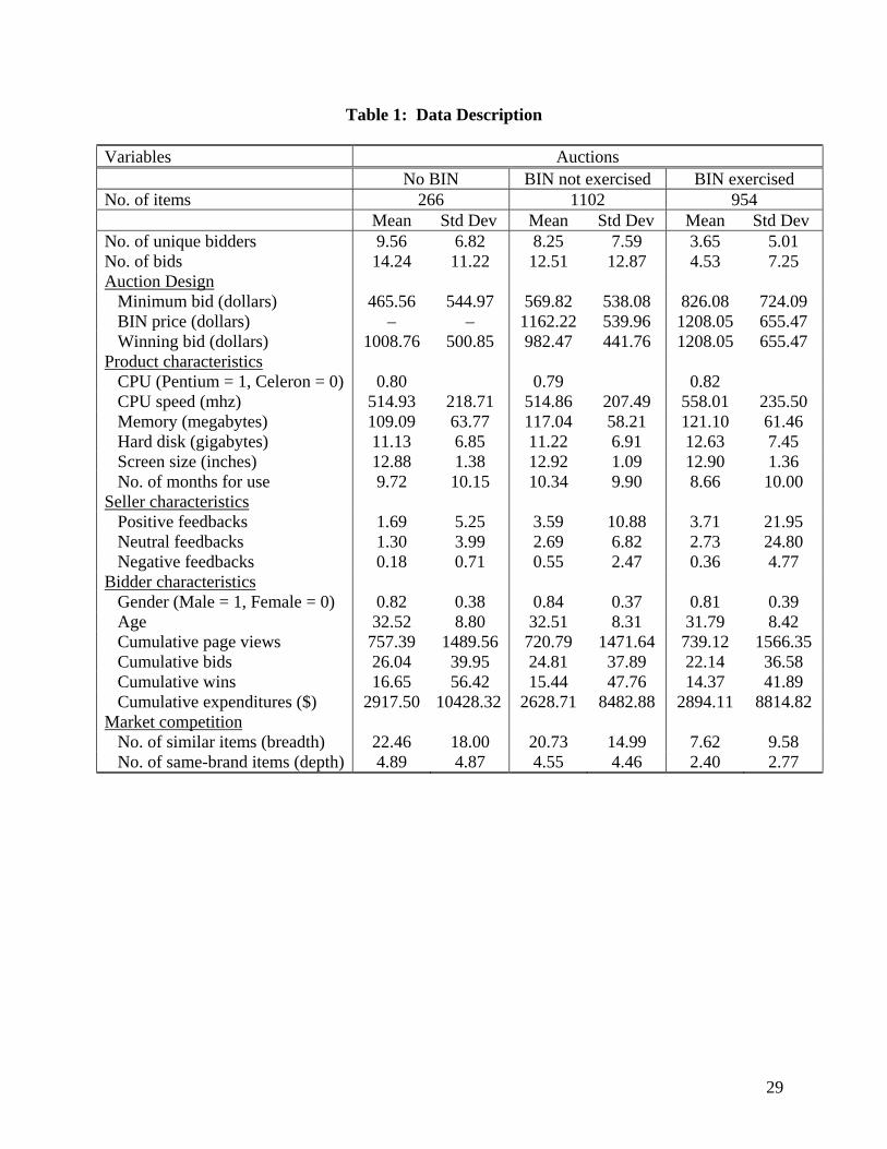
Table 1: Data Description Variables Auctions No BIN BIN not exercised BIN exercised No. of items 266 1102 954 Mean Std Dev Mean Std Dev Mean Std Dev No. of unique bidders 9.56 6.82 8.25 7.59 3.65 5.01 No. of bids 14.24 11.22 12.51 12.87 4.53 7.25 Auction Design Minimum bid (dollars) 465.56 544.97 569.82 538.08 826.08 724.09 BIN price (dollars) – – 1162.22 539.96 1208.05 655.47 Winning bid (dollars) 1008.76 500.85 982.47 441.76 1208.05 655.47 Product characteristics CPU (Pentium = 1, Celeron = 0) 0.80 0.79 0.82 CPU speed (mhz) 514.93 218.71 514.86 207.49 558.01 235.50 Memory (megabytes) 109.09 63.77 117.04 58.21 121.10 61.46 Hard disk (gigabytes) 11.13 6.85 11.22 6.91 12.63 7.45 Screen size (inches) 12.88 1.38 12.92 1.09 12.90 1.36 No. of months for use 9.72 10.15 10.34 9.90 8.66 10.00 Seller characteristics Positive feedbacks 1.69 5.25 3.59 10.88 3.71 21.95 Neutral feedbacks 1.30 3.99 2.69 6.82 2.73 24.80 Negative feedbacks 0.18 0.71 0.55 2.47 0.36 4.77 Bidder characteristics Gender (Male = 1, Female = 0) 0.82 0.38 0.84 0.37 0.81 0.39 Age 32.52 8.80 32.51 8.31 31.79 8.42 Cumulative page views 757.39 1489.56 720.79 1471.64 739.12 1566.35 Cumulative bids 26.04 39.95 24.81 37.89 22.14 36.58 Cumulative wins 16.65 56.42 15.44 47.76 14.37 41.89 Cumulative expenditures ($) 2917.50 10428.32 2628.71 8482.88 2894.11 8814.82 Market competition No. of similar items (breadth) 22.46 18.00 20.73 14.99 7.62 9.58 No. of same-brand items (depth) 4.89 4.87 4.55 4.46 2.40 2.77

29

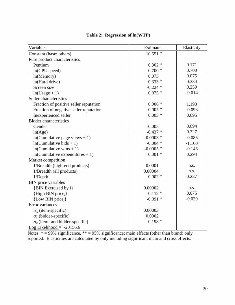
Table 2: Regression of ln(WTP) Variables Estimate Elasticity Constant (base: others) 10.551 * Pure product characteristics Pentium 0.302 * 0.171 ln(CPU speed) 0.700 * 0.700 ln(Memory) 0.075 0.075 ln(Hard drive) 0.333 * 0.334 Screen size -0.224 * 0.250 ln(Usage + 1) 0.075 * -0.014 Seller characteristics Fraction of positive seller reputation 0.006 * 1.193 Fraction of negative seller reputation -0.005 * -0.093 Inexperienced seller 0.003 * 0.695 Bidder characteristics Gender -0.005 0.094 ln(Age) -0.437 * 0.327 ln(Cumulative page views + 1) -0.0003 * -0.085 ln(Cumulative bids + 1) -0.004 * -1.160 ln(Cumulative wins + 1) -0.0005 * -0.146 ln(Cumulative expenditures + 1) 0.001 * 0.294 Market competition 1/Breadth (high-end products) 0.0001 n.s. 1/Breadth (all products) 0.00004 n.s. 1/Depth 0.002 * 0.237 BIN price variables {BIN Exercised by i} 0.00002 n.s. {High BIN pricej} 0.112 * 0.075 {Low BIN pricej} -0.091 * -0.029 Error variances ση (item-specific) 0.00003 σξ (bidder-specific) 0.0002 σε (item- and bidder-specific) 0.198 * Log Likelihood = -20156.6 Notes: * = 99% significance, ** = 95% significance; main effects (other than brand) only reported. Elasticities are calculated by only including significant main and cross effects.

30

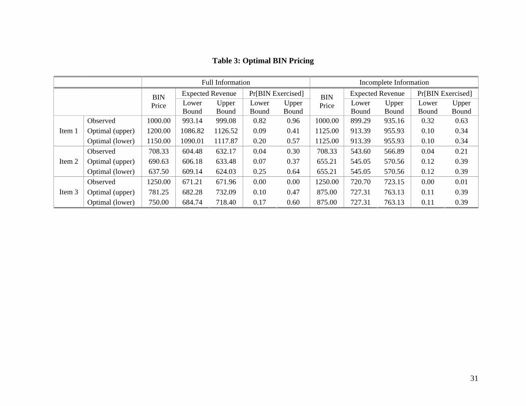
Table 3: Optimal BIN Pricing

Full Information Incomplete Information Expected Revenue Pr[BIN Exercised] Expected Revenue Pr[BIN Exercised]

BIN Price Lower

Bound Upper Bound

Lower Bound

Upper Bound

BIN Price Lower

Bound Upper Bound

Lower Bound

Upper Bound

Observed 1000.00 993.14 999.08 0.82 0.96 1000.00 899.29 935.16 0.32 0.63Optimal (upper) 1200.00 1086.82 1126.52 0.09 0.41 1125.00 913.39 955.93 0.10 0.34Item 1 Optimal (lower) 1150.00 1090.01 1117.87 0.20 0.57 1125.00 913.39 955.93 0.10 0.34Observed 708.33 604.48 632.17 0.04 0.30 708.33 543.60 566.89 0.04 0.21Optimal (upper) 690.63 606.18 633.48 0.07 0.37 655.21 545.05 570.56 0.12 0.39Item 2 Optimal (lower) 637.50 609.14 624.03 0.25 0.64 655.21 545.05 570.56 0.12 0.39Observed 1250.00 671.21 671.96 0.00 0.00 1250.00 720.70 723.15 0.00 0.01Optimal (upper) 781.25 682.28 732.09 0.10 0.47 875.00 727.31 763.13 0.11 0.39Item 3 Optimal (lower) 750.00 684.74 718.40 0.17 0.60 875.00 727.31 763.13 0.11 0.39

31

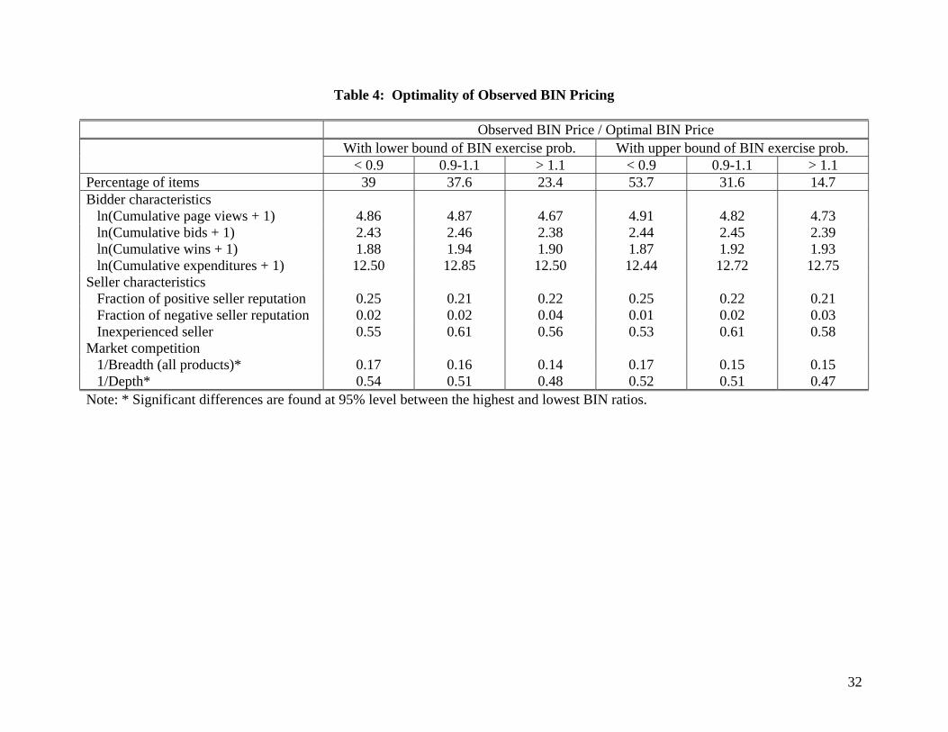
Table 4: Optimality of Observed BIN Pricing Observed BIN Price / Optimal BIN Price With lower bound of BIN exercise prob. With upper bound of BIN exercise prob. < 0.9 0.9-1.1 > 1.1 < 0.9 0.9-1.1 > 1.1Percentage of items 39 37.6 23.4 53.7 31.6 14.7Bidder characteristics ln(Cumulative page views + 1) 4.86 4.87 4.67 4.91 4.82 4.73 ln(Cumulative bids + 1) 2.43 2.46 2.38 2.44 2.45 2.39 ln(Cumulative wins + 1) 1.88 1.94 1.90 1.87 1.92 1.93 ln(Cumulative expenditures + 1) 12.50 12.85 12.50 12.44 12.72 12.75 Seller characteristics Fraction of positive seller reputation 0.25 0.21 0.22 0.25 0.22 0.21 Fraction of negative seller reputation 0.02 0.02 0.04 0.01 0.02 0.03 Inexperienced seller 0.55 0.61 0.56 0.53 0.61 0.58Market competition 1/Breadth (all products)* 0.17 0.16 0.14 0.17 0.15 0.15 1/Depth* 0.54 0.51 0.48 0.52 0.51 0.47Note: * Significant differences are found at 95% level between the highest and lowest BIN ratios.

32