The Evolution of the Global Value Chain

The Evolution of the Global Value Chain

by

Yibei Liu

B.A., Beijing Normal University, 2006

M.A., University of Denver, 2008

M.A., University of Colorado at Boulder, 2010

A thesis submitted to the

Faculty of the Graduate School of the

University of Colorado in partial fulfillment

of the requirements for the degree of

Doctor of Philosophy

Department of Economics

2014

This thesis entitled:The Evolution of the Global Value Chain

written by Yibei Liuhas been approved for the Department of Economics

James Markusen

Keith Maskus

Date

The final copy of this thesis has been examined by the signatories, and we find that both thecontent and the form meet acceptable presentation standards of scholarly work in the above

mentioned discipline.

Liu, Yibei (Ph.D., Economics)

The Evolution of the Global Value Chain

Thesis directed by Professor James Markusen

Production processes are increasingly fragmented geographically, and the performance of

production tasks is spread across countries. As multinational production progresses, an intriguing

phenomenon arises which is referred to as countries and firms “moving up the global value chain.”

While many people may have an informal understanding of what it means, testable definitions and

examinations of the dynamics are lacking.

My dissertation aims to provide a unified framework to address the meaning and mechanism

of the dynamics of global production and value chain. Task-based theoretical models are developed

to explore and characterize the dynamics, which arise from learning-by-doing. Using firm-level

data, empirical support for the important theoretical predictions is found. The model is further

extended to incorporate the innovation effect, which explains the rising phenomenon of reshoring.

Following the first and second chapter for introduction and literature review, in Chapter 3, I

develop a dynamic task-based model of multinational production. The technology of producing a

final good is modeled as a spectrum of tasks ranked by their degree of technological sophistication.

The global value chain of an industry is thus described as a sequence of tasks that may be spread

across countries, with each task adding value to the final good. “Moving up the global value chain”

is then defined as an upgrading in the set of tasks that a country, an industry, or a firm conducts.

The basic model features the critical role of learning-by-doing in the dynamic production

process. Initially, developed countries (the North) offshore simple tasks to developing countries

(the South). The South may receive tasks beyond its technological capability. By conducting the

“beyond” tasks, the South improves its efficiency on relatively sophisticated tasks. This learning-by-

doing effect enables more complex tasks to be offshored in the next period. This process continues

until the Southern technological capability matches the set of tasks offshored. Both types of coun-

iv

tries move up the global value chain during this process – the South conducts additional and harder

tasks, while the North concentrates on fewer but the most highly sophisticated activities. The evo-

lution of multinational production is characterized by the task offshoring threshold moving up to

its steady state, with the movement pace slowing down over time – thus a concave-shaped path.

The dynamics of other economic aspects, including wage rates and national welfare, are discussed.

In Chapter 4, I develop the dynamic theory of global production within a monopolistic

competition framework. Products are differentiated by variety, with each variety being produced

by a multinational firm. Countries and firms move up the global value chain due to firms’ learning-

by-doing effects, as the Southern subsidiaries engage in a wider range of and more sophisticated

tasks, while the Northern counterparts do fewer but more complex activities. The number of

varieties increases and displays a converging pattern of growth during the evolution process, and

this expansion at the extensive margin is the main source of welfare gains for both countries.

The situation under autarky and the dynamic gains from offshoring are examined. Under

monopolistic competition, the South may experience a welfare loss in the short run upon participat-

ing in global production. However, in the long run, the learning-by-doing effect will lead the South

to be better off than its autarky situation. Meanwhile, the North enjoys a higher level of welfare

at the beginning of joining global production, and the gain continues in the long run. Hence, both

types of countries get rewarded from offshoring, though their paths are quite different.

The task-based theory predicts that as multinational production evolves, the Southern coun-

try’s share of value added in total value of industrial output increases over time, while the growth

rate declines – thus a concave-shaped path. In Chapter 5, a micro-founded approach is applied to

test the dynamics of the value-added ratio (VR) of global production contributed by the South. By

using a subsidiary-level dataset on China’s multinational operation spanning 10 years, the evolution

pattern of industry-level VR is examined. The results show that convergence evidences are present,

and the industrial VR dynamics are mainly driven by changes within multinational subsidiaries.

Chapter 6 extends the model to incorporate innovation in developed home countries. Task al-

location depends on countries’ relative efficiency of conducting tasks. When both countries improve

v

domestic technologies simultaneously – one through learning and the other through innovation, the

dynamics of multinational production are determined by the countries’ relative speed of technology

improvement. Both offshoring expansion and reshoring may occur, where reshoring refers to the

phenomenon that previously offshored tasks return to their originating home countries.

Dedication

I wish to dedicate this dissertation to my beloved family, for your continued support and

encouragement.

vii

Acknowledgements

I would like to thank many people who have helped me through the completion of this dis-

sertation. The first is my advisor and committee chair, Prof. James Markusen, who is always

enthusiastic, honest and supportive, both professionally and personally. Thank you for your en-

couragement and immense knowledge. I would like to thank my co-advisor, Prof. Wolfgang Keller.

I have learned a lot from your dedication to economic research and your rigorous scholarship. This

dissertation would not have been possible without the mentorship of you both.

I am indebted to my dynamic and intelligent committee members, Prof. Keith Maskus, Prof.

Chrystie Burr, and Prof. Edward Balistreri. Thank you for your insightful comments, questions

and support. I would also like to thank the Department of Economics at CU-Boulder for funding

my time at CU-Boulder.

My sincere thanks also go to: Thibault Fally, my course instructor of International Trade;

and Ben Li, for bouncing ideas with me and always being supportive as both friend and colleague.

I would like to ackowledge the professors and other professionals who trained me or inspired me in

some way. Some of these include: Tania Barham, Martin Boileau, Brian Cadena, Yongmin Chen,

Charles de Bartolome, Xiaodong Liu, Terra McKinnish, Edward Morey, Scott Savage, Donald

Waldman and Jeffrey Zax; and the seminar participants at CU-Boulder, the Midwest International

Economics Meeting, Oregon State University, Yale-NUS College and the University of Auckland.

I am beyond grateful to, thus very special thanks to, my family, for their unconditional love

and support throughout my life. My final thanks go to my friends, who are now scattered around

the world, for the late night phone calls and their coffee dates.

viii

Contents

Chapter

1 Introduction 1

1.1 A Dynamic Theory of Global Production: A Task-Based Perspective . . . . . . . . . 2

1.2 The Dynamics of Global Value Chain in Monopolistic Competition . . . . . . . . . . 3

1.3 Moving Up the Global Value Chain: Evidence from China . . . . . . . . . . . . . . . 4

1.4 Innovation in the Home Country: An Extension . . . . . . . . . . . . . . . . . . . . . 5

2 Review of the Literature 6

3 A Dynamic Theory of Global Production: A Task-Based Perspective 11

3.1 Set-up of the Model . . . . . . . . . . . . . . . . . . . . . . . . . . . . . . . . . . . . 13

3.1.1 Production . . . . . . . . . . . . . . . . . . . . . . . . . . . . . . . . . . . . . 13

3.1.2 Learning-by-Doing . . . . . . . . . . . . . . . . . . . . . . . . . . . . . . . . . 14

3.2 Instantaneous Equilibrium and Steady State of Multinational Production . . . . . . 16

3.2.1 Instantaneous Equilibrium . . . . . . . . . . . . . . . . . . . . . . . . . . . . . 16

3.2.2 Steady State . . . . . . . . . . . . . . . . . . . . . . . . . . . . . . . . . . . . 17

3.3 Transition Dynamics of Task Offshoring . . . . . . . . . . . . . . . . . . . . . . . . . 18

3.3.1 Transition Dynamics of Task Offshoring with an Initially Efficient South . . . 18

3.3.2 Transition Dynamics of Task Offshoring with Learning-by-Doing . . . . . . . 19

3.4 Dynamics of National Welfare and Gains from Offshoring . . . . . . . . . . . . . . . 23

3.4.1 Dynamics of Wage Rates . . . . . . . . . . . . . . . . . . . . . . . . . . . . . 24

ix

3.4.2 Dynamics of Output . . . . . . . . . . . . . . . . . . . . . . . . . . . . . . . . 25

3.4.3 Dynamics of National Welfare . . . . . . . . . . . . . . . . . . . . . . . . . . . 25

3.5 Gains from Offshoring . . . . . . . . . . . . . . . . . . . . . . . . . . . . . . . . . . . 29

3.5.1 Welfare under Autarky . . . . . . . . . . . . . . . . . . . . . . . . . . . . . . 30

3.5.2 Gains from Offshoring with Learning-by-Doing . . . . . . . . . . . . . . . . . 30

3.6 Concluding Remarks . . . . . . . . . . . . . . . . . . . . . . . . . . . . . . . . . . . . 32

4 The Dynamics of Global Value Chain in Monopolistic Competition 33


4.1.1 Preference . . . . . . . . . . . . . . . . . . . . . . . . . . . . . . . . . . . . . . 35

4.1.2 Product Market . . . . . . . . . . . . . . . . . . . . . . . . . . . . . . . . . . 35

4.1.3 Production . . . . . . . . . . . . . . . . . . . . . . . . . . . . . . . . . . . . . 36


4.2 Instantaneous Equilibrium and Steady State of Multinational Production . . . . . . 39


4.2.2 Steady State . . . . . . . . . . . . . . . . . . . . . . . . . . . . . . . . . . . . 41

4.3 Transition Dynamics . . . . . . . . . . . . . . . . . . . . . . . . . . . . . . . . . . . . 42

4.3.1 Task Dynamics . . . . . . . . . . . . . . . . . . . . . . . . . . . . . . . . . . . 44

4.3.2 Variety Dynamics . . . . . . . . . . . . . . . . . . . . . . . . . . . . . . . . . 49

4.3.3 Dynamics of Factor Income . . . . . . . . . . . . . . . . . . . . . . . . . . . . 51

4.3.4 Dynamics of National Welfare . . . . . . . . . . . . . . . . . . . . . . . . . . . 53

4.3.5 Extreme-End Evolution . . . . . . . . . . . . . . . . . . . . . . . . . . . . . . 58

4.3.6 Static Equilibrium Cases . . . . . . . . . . . . . . . . . . . . . . . . . . . . . 63

4.4 Gains from Offshoring . . . . . . . . . . . . . . . . . . . . . . . . . . . . . . . . . . . 64

4.4.1 Equilibrium under Autarky . . . . . . . . . . . . . . . . . . . . . . . . . . . . 64

4.4.2 Gains from Normal Offshoring . . . . . . . . . . . . . . . . . . . . . . . . . . 66

4.4.3 Gains from Extreme-End Offshoring . . . . . . . . . . . . . . . . . . . . . . . 68

x


5 Moving Up the Global Value Chain: Evidence from China 72

5.1 Review of the Theoretical Prediction . . . . . . . . . . . . . . . . . . . . . . . . . . . 73

5.2 Empirical Approach . . . . . . . . . . . . . . . . . . . . . . . . . . . . . . . . . . . . 74

5.2.1 Data on Multinational Operations: the Usage . . . . . . . . . . . . . . . . . . 74

5.2.2 Convergence of VRS . . . . . . . . . . . . . . . . . . . . . . . . . . . . . . . . 75

5.2.3 Two Margins of Changes . . . . . . . . . . . . . . . . . . . . . . . . . . . . . 76

5.3 Data Description . . . . . . . . . . . . . . . . . . . . . . . . . . . . . . . . . . . . . . 77

5.4 Empirical Results . . . . . . . . . . . . . . . . . . . . . . . . . . . . . . . . . . . . . . 79


6 An Extension: Multinational Production, Innovation, and the Dynamics of Task Allocation 90


6.1.1 Production . . . . . . . . . . . . . . . . . . . . . . . . . . . . . . . . . . . . . 91

6.1.2 Innovation . . . . . . . . . . . . . . . . . . . . . . . . . . . . . . . . . . . . . . 92


6.2 Instantaneous Equilibrium of Multinational Production . . . . . . . . . . . . . . . . 94


6.2.2 The Wage-Equalization Threshold . . . . . . . . . . . . . . . . . . . . . . . . 95

6.3 The Evolution Dynamics: An Initially Efficient South . . . . . . . . . . . . . . . . . 96

6.3.1 Evolution Dynamics: Equal Paces of Technological Progress . . . . . . . . . . 96

6.3.2 Evolution Dynamics: Fast Northern Innovation . . . . . . . . . . . . . . . . . 97

6.3.3 Evolution Dynamics: Fast Southern Learning . . . . . . . . . . . . . . . . . . 101

6.4 The Evolution Dynamics: An Initially Inefficient South . . . . . . . . . . . . . . . . 102

6.4.1 Evolution Dynamics: Equal Paces of Technological Progress . . . . . . . . . . 103

6.4.2 Evolution Dynamics: Fast Northern Innovation . . . . . . . . . . . . . . . . . 105

6.4.3 Evolution Dynamics: Fast Southern Learning . . . . . . . . . . . . . . . . . . 109

xi


Bibliography 114

Appendix

A Derivations for Chapter 3 120

A.1 Transition Dynamics of Task Offshoring . . . . . . . . . . . . . . . . . . . . . . . . . 120

A.1.1 Evolution of Technology Stock with Learning-by-Doing . . . . . . . . . . . . 120

A.1.2 Evolution of Offshoring Threshold with Learning-by-Doing . . . . . . . . . . 121

A.2 Dynamics of National Welfare and Gains from Offshoring . . . . . . . . . . . . . . . 121

A.2.1 Evolution of Output with Learning-by-Doing . . . . . . . . . . . . . . . . . . 121

A.2.2 Evolution of Southern Welfare with Learning-by-Doing . . . . . . . . . . . . . 122

A.2.3 Evolution of Northern Welfare with Learning-by-Doing . . . . . . . . . . . . . 123

B Derivations for Chapter 4 124

B.1 Transition Dynamics of Task Offshoring . . . . . . . . . . . . . . . . . . . . . . . . . 124

B.1.1 Evolution of Technology Stock with Learning-by-Doing . . . . . . . . . . . . 124

B.1.2 Evolution of Offshoring Threshold with Learning-by-Doing . . . . . . . . . . 125

B.2 Evolution of Number of Variety with Learning-by-Doing . . . . . . . . . . . . . . . . 125

B.2.1 Derivation of (4.30): dJ(t)dt > 0 . . . . . . . . . . . . . . . . . . . . . . . . . . 125

B.2.2 Derivation of (4.30): d2J(t)dt2

< 0 . . . . . . . . . . . . . . . . . . . . . . . . . . 125

B.3 Evolution of Per-Brand Output with Learning-by-Doing . . . . . . . . . . . . . . . . 125

B.3.1 Derivation of Per-Brand Output – (4.33) . . . . . . . . . . . . . . . . . . . . . 125

B.3.2 Time Dynamics of Per-Brand Output . . . . . . . . . . . . . . . . . . . . . . 126

B.4 Dynamics of National Welfares . . . . . . . . . . . . . . . . . . . . . . . . . . . . . . 127

B.4.1 Derivation of dUS(t)dt . . . . . . . . . . . . . . . . . . . . . . . . . . . . . . . . 127

B.4.2 Dynamics of Northern Welfare UN (t) . . . . . . . . . . . . . . . . . . . . . . . 127

xii

B.5 Extreme-End Evolution . . . . . . . . . . . . . . . . . . . . . . . . . . . . . . . . . . 128

B.5.1 Derivation of (4.40) . . . . . . . . . . . . . . . . . . . . . . . . . . . . . . . . 128

B.5.2 Derivation of dY (t)′

dt . . . . . . . . . . . . . . . . . . . . . . . . . . . . . . . . . 128

B.6 Northern Gains from Offshoring under Complete Offshoring . . . . . . . . . . . . . . 128

C Derivations for Chapter 6 129

C.1 The Evolution Dynamics: An Initially Efficient South, Fast Northern Innovation . . 129

C.2 The Evolution Dynamics: An Initially Inefficient South . . . . . . . . . . . . . . . . 129

C.2.1 Evolution Dynamics: Fast Northern Innovation . . . . . . . . . . . . . . . . . 129

C.2.2 Evolution Dynamics: Fast Southern Learning . . . . . . . . . . . . . . . . . . 130

xiii

Tables

Table

5.1 Summary Statistics of Multinational Subsidiaries . . . . . . . . . . . . . . . . . . . . 77

5.2 Change in VR and the Two Margins . . . . . . . . . . . . . . . . . . . . . . . . . . . 80

5.3 Industry Description . . . . . . . . . . . . . . . . . . . . . . . . . . . . . . . . . . . . 81

5.4 Overall ∆VR of Multinational Operation . . . . . . . . . . . . . . . . . . . . . . . . 83

5.5 Within-Subsidiary Margin of ∆VR, Multinational Operation . . . . . . . . . . . . . 84

5.6 Cross-Subsidiary Margin of ∆VR, Multinational Operation . . . . . . . . . . . . . . 85

5.7 ∆VR and its Two Margins, Multinational Operations, Various Initial Years . . . . . 87

5.8 ∆VR and its Two Margins, Multinational Operations, Skill Intensity Measures . . . 88

5.9 ∆VR and its Two Margins, Local Production and HMT-Owned Operations . . . . . 89

xiv

Figures

Figure

3.1 Unit Labor Requirement Evolution with Learning-by-Doing . . . . . . . . . . . . . . 15

3.2 Dynamics of Task Offshoring: an Initially Efficient South . . . . . . . . . . . . . . . 20

3.3 Initial Task Offshoring: an Initially Inefficient South . . . . . . . . . . . . . . . . . . 21

3.4 Dynamics of Task Offshoring: an Initially Inefficient South . . . . . . . . . . . . . . 23

3.5 Dynamics of Wage Rates . . . . . . . . . . . . . . . . . . . . . . . . . . . . . . . . . . 24

3.6 Dynamics of Output . . . . . . . . . . . . . . . . . . . . . . . . . . . . . . . . . . . . 26

3.7 Dynamics of Southern Welfare . . . . . . . . . . . . . . . . . . . . . . . . . . . . . . 27

3.8 Dynamics of Northern Welfare . . . . . . . . . . . . . . . . . . . . . . . . . . . . . . 29

4.1 Unit Labor Requirement Evolution with Learning-by-Doing . . . . . . . . . . . . . . 38

4.2 Initial Task Offshoring . . . . . . . . . . . . . . . . . . . . . . . . . . . . . . . . . . . 45

4.3 Dynamics of Task Offshoring . . . . . . . . . . . . . . . . . . . . . . . . . . . . . . . 47

4.4 Dynamics of Task Offshoring: Simulations . . . . . . . . . . . . . . . . . . . . . . . . 48

4.5 Dynamics of Variety . . . . . . . . . . . . . . . . . . . . . . . . . . . . . . . . . . . . 51

4.6 Dynamics of Wage Rates . . . . . . . . . . . . . . . . . . . . . . . . . . . . . . . . . . 52

4.7 Dynamics of Per-Brand Output . . . . . . . . . . . . . . . . . . . . . . . . . . . . . . 54

4.8 Dynamics of National Welfare: Simulations . . . . . . . . . . . . . . . . . . . . . . . 57

4.9 Task Dynamics under Extreme-End Evolution . . . . . . . . . . . . . . . . . . . . . . 59

4.10 Dynamics of Wage Rates and Number of Varieties . . . . . . . . . . . . . . . . . . . 60

xv

4.11 Dynamics of Output and Welfares . . . . . . . . . . . . . . . . . . . . . . . . . . . . 62

4.12 Welfare Gains from Offshoring: Normal Evolution . . . . . . . . . . . . . . . . . . . 69

4.13 Welfare Gains from Offshoring: Complete Offshoring . . . . . . . . . . . . . . . . . . 70

5.1 Value-Added/Output Ratio Growth . . . . . . . . . . . . . . . . . . . . . . . . . . . 78

5.2 Decomposition of VR Changes . . . . . . . . . . . . . . . . . . . . . . . . . . . . . . 79

6.1 Dynamics of Task Offshoring: Equal Paces of Technological Progress . . . . . . . . . 97

6.2 Dynamics of Task Offshoring: Fast Northern Innovation . . . . . . . . . . . . . . . . 99

6.3 Evolution of Offshoring Threshold: Fast Northern Innovation . . . . . . . . . . . . . 100

6.4 Dynamics of Task Offshoring: Fast Southern Learning . . . . . . . . . . . . . . . . . 102

6.5 Dynamics of Task Offshoring: Equal Paces of Technological Progress . . . . . . . . . 104

6.6 Dynamics of Task Offshoring: Fast Northern Innovation . . . . . . . . . . . . . . . . 106

6.7 Evolution of Offshoring Threshold: A Large South, Fast Northern Innovation . . . . 108

6.8 Evolution of Offshoring Threshold: A Small South, Fast Northern Innovation . . . . 109

6.9 Dynamics of Task Offshoring: Fast Southern Learning . . . . . . . . . . . . . . . . . 110

6.10 Evolution of Offshoring Threshold: Fast Southern Learning . . . . . . . . . . . . . . 112

Chapter 1

Introduction

Currently, global economic activities feature a complex multinational production network

with a prominent role played by international task trade, as production processes become increas-

ingly fragmented geographically and the performance of production tasks is spread across the globe.

It is not unusual for a final good to have components or technology produced in a high-income coun-

try, which are then exported to a lower-income country where final assembly occurs, with the final

product exported back to the originating high-income country.

Over time, an intriguing phenomenon arises which is widely referred to as countries and firms

“moving up along the value chain of global production.” The phrase is used, for instance, (1) in

describing the fact that the Brazilian automotive industry, starting with an assembly line built by

General Motors, now develops new car models and has become among the world’s largest vehicle

producers; (2) as the reason why Asian-Tiger economies experienced rapid industrialization and

maintained high growth rates for decades after World War II; and (3) as the recipe for OECD

countries to stay competitive in the global environment. While many people may have an informal

understanding of what “moving up the global value chain” means, testable definitions and exam-

inations of mechanisms of the dynamics involved in this process are lacking. In particular, what

is the chain variable? Who is on the chain? Why do countries and firms claim they move up the

chain altogether, even if they are at quite different development stages? And how do countries and

firms move along the chain?

Exploring these issues, my dissertation aims to provide a unified framework to address the

2

meaning and mechanism of the dynamics of global production. This chapter, as a brief introduction,

will provide an overview of the dissertation. After a review of literature in Chapter 2, Chapter 3

introduces the basic task-based model of multinational production, which is briefly outlined here

in Section 1.1. Section 1.2 provides an overview of the dynamic theory of global production in

monopolistic competition, which is presented in Chapter 4. Section 1.3 overviews the empirical

investigation with subsidiary-level data on China’s multinational operation. A theoretical extension

incorporating innovation into the framework is briefly introduced in Section 1.4.

1.1 A Dynamic Theory of Global Production: A Task-Based Perspective

In Chapter 3 of my dissertation, I develop a unified dynamic task-based theory on global

production with the technology for producing a final good modeled as a spectrum of production

tasks which are ranked by their degree of technological sophistication. Moving up the global value

chain is then given a specific definition as an upgrading in the set of tasks that a country, an

industry or a firm conducts. For different countries and firms, the upgrading pattern may vary.

The model features the role of learning-by-doing in the production process, within a perfect

competition framework. At the start, developed countries (the North) offshore relatively simple

tasks to developing countries (the South). The South acquires certain tasks that are moderately

beyond its technological capability. These tasks provide the South with opportunities to improve

its production technology through the learning-by-doing effect. This enables the South to carry

out the relatively sophisticated tasks more efficiently, which then leads to more complex tasks

being offshored in the next period. This self-reinforcing process continues until the technological

capability of the South matches the tasks offshored – the long-run steady state. Over time, the

Southern coverage of the task spectrum becomes increasingly wide and sophisticated, while the

Northern coverage, although narrower over time, concentrates on the tasks involving the highest

degree of sophistication.

The movement of global production equilibrium is characterized by the task threshold of

offshoring moving toward its steady state, with the movement pace slowing down over time. The

3

evolution of the Southern task scope thus displays a concave-shaped time path, with the steady

state being the upper bound. During this process, other aspects of global production also converge

to their long-run steady states. The time dynamics of wage rates, output and national welfare levels

are examined. Gains from offshoring are also analyzed. The findings indicate that compared with

autarky, both the South and the North gain from participating in global production and evolving

with offshoring and learning dynamics. While the short-run gain presents for both, the long-run

gain at the steady state is mainly for developing countries.

1.2 The Dynamics of Global Value Chain in Monopolistic Competition

Based on the basic model, I further develop the dynamic theory of global production within

a monopolistic competition framework in Chapter 4. Products are differentiated by brand, with

each brand being produced by a single firm. With offshoring, firms become multinational enter-

prises (MNEs), with relatively simple tasks being offshored to the Southern subsidiaries initially.

When both countries conduct offshorable tasks and with a positive Southern learning effect, more

and increasingly sophisticated tasks are reallocated from the North to the South, with the North

concentrating on the high-end tasks and non-offshorable activities. Countries and firms move up

the global value chain, as the Southern subsidiaries do more and harder tasks, and the Northern

counterparts do fewer but more complex tasks. Meanwhile, the number of varieties increases and

displays a converging pattern of growth. The expansion at the extensive margin serves as the main

source of welfare gains for both countries.

What is interesting here is that with non-offshorable activities being necessary and costly for

firms, under certain circumstances, the North may not be participating in any offshorable tasks.

Rather, all these tasks are offshored to the South. In this situation, if the Southern subsidiaries

have opportunities to learn through conducting tasks beyond their technological capabilities, both

countries may be better off over time in terms of consumer welfare.

The autarky situation and dynamic gains from offshoring are examined in this chapter. The

gains from offshoring, compared with autarky, can be decomposed into two effects: 1) the variety

4

effect (the extensive margin), with the number of varieties enjoyed by consumers being different

from the autarky case, and 2) the consumption effect (the intensive margin), with the per-brand

consumption level being changed. The interaction between the two effects determines the national

welfare gains from offshoring. It is found that the variety effect is constantly positive for both

countries, while the consumption effect is not definitely constantly positive. Combining both effects,

different from the situation under perfect competition discussed in the basic model, the developing

country here may experience a short-run welfare loss upon participating in global production.

However, in the long run, the learning effect will lead the South to be better off than its autarky

situation. Meanwhile, the North enjoys a higher welfare level since the beginning of joining global

production, and the gain continues in the long-run. Therefore, although both types of countries

will be rewarded from joining the multinational production chain, the paths can be quite different.

1.3 Moving Up the Global Value Chain: Evidence from China

A central prediction of the theories is that global production converges to a steady state where

no further offshoring occurs. During this evolution process, the national contribution of industrial

value-added is dynamically redistributed between countries – the Southern part increases while

the Northern part decreases, and the speed of redistribution declines over time. ”Moving up the

global value chain” thus translates into an increasing Southern share of value added in total value

of industrial output over time, while the speed of growth declines gradually.

An empirical approach is thus applied to examine the dynamics of Southern share of total

value-added in Chapter 5, and it can be applied to firm-level data from any developing host country.

In the approach, multinational subsidiaries in a Southern country are grouped into industries that

are considered as multinational industries, and multinational subsidiaries themselves are viewed as

collections of tasks. A growth and convergence of the value-added ratio (VR, value-added divided

by total value) of multinational industries would support the theoretical predictions on value-added

share dynamics.

Subsidiaries are not weightless, and therefore their weights may drive industry-level VR

5

to change even with no VR change within them. To determine whether the VR growth and

convergence of multinational industries are essentially driven by those of subsidiaries, I decompose

the VR change of each multinational industry into two margins – a within-subsidiary margin and a

cross-subsidiary margin, and examine whether each of the two margins, as well as the industry-level

VR change itself, is converging. Using this approach, I examine subsidiary-level data on China’s

multinational operation over ten years (1998-2007). Convergence is found at the industry level,

and it is primarily driven by the within-subsidiary margin, which is consistent with the theory.

1.4 Innovation in the Home Country: An Extension

The reshoring phenomenon has been rising recently: production capacities and facilities start

returning to developed countries from developing countries where they were previously offshored.

One important motivation behind this trend is that developed countries’ advantages in production

efficiency are able to offset their disadvantages in factor prices. One of the essential reasons here

is that the Northern countries keep innovating on production technologies, which outpaces the

corresponding improvements taking place in the South. In Chapter 6, I incorporate the important

factor of technology improvement – innovation – into the analysis framework of global value chain.

With technology progresses in both countries – innovation in the North and learning in

the South, the interaction between the pace of innovation and that of learning determines the

organization dynamics of global production. The model provides predictions and explanations for

the dynamics of offshoring and reshoring. Both offshoring expansion and reshoring are possible

under this enriched framework, depending upon how the countries’ relative production efficiency

may change over time.

Chapter 2

Review of the Literature

This chapter presents an overview of the existing research on global production and value

chain, from the perspective of international trade. The literature has helped shape the theoretical

and empirical position developed in this study, and it serves as a lens through which to view this

research in a comprehensive contextual framework. Contributions of this research to the literature

are thus discussed accordingly in this chapter.

There is a growing literature on multinational production that views global integration as

increasingly marked by task trade, and the global chain of production is thus modeled as a collection

of offshorable tasks or a continuum of stages of production. Early examples include Dixit and

Grossman (1982) and Feenstra and Hanson (1996b, 1997).1 More recent works further explore

issues such as the effects of heterogeneous offshoring costs (e.g., Grossman and Rossi-Hansberg,

2008, 2012), the optimal allocation of ownership rights along the value chain (e.g., Antras and Chor,

2013), and the influence of technological change on the interdependence of countries participating

in the global supply chain (e.g., Costinot et al., 2013).2 Sharing with this body of literature that

global production is considered and analyzed in a task-based framework, I formulate the dynamic

theoretical framework of global value chain in this study, in which the location of value added

and task trade are endogenously determined. As discussed in the literature, there are various

configurations of production processes, such as the “spider” and “snake” described in Baldwin and

1 Other early related works such as Dornbusch, Fischer, and Samuelson (1977, 1980) have studied trade theoriesbased on a continuum of tradable goods.

2 Other important task- or stage-based works include Carluccio and Fally (2013), Yi (2003), Baldwin and Venables(2013), and Baldwin and Robert-Nicoud (2014).

7

Venables (2013), and studies on production-chain issues often assume that tasks and/or stages

of production are sequential in nature (e.g., Costinot et al., 2013 and Antras and Chor, 2013).

As models assuming task sequentiality provide sharp insights into the production-chain issues,

particularly for the “snake” type of production process, it is desirable that the global production and

value chain be understood and interpreted in a generalized way, without depending on any particular

pattern of production process. To capture this idea, my models set no specific requirement for the

sequence of task- or stage-completion, with tasks being ranked by their degree of technological

sophistication in the framework.3 Thus, the specific organization pattern of a production process

is less a concern when using the framework presented in this study to examine and explain value-

chain issues.

The theoretical framework presented in this study features the critical role of dynamic

learning-by-doing in the production process, and it provides rich descriptions on how global pro-

duction may evolve and the resulted dynamic effects of this process on various economic aspects.

In the existing literature, learning-by-doing has long been viewed as a central driver for growth

and upgrading at various economic levels. Since Arrow (1962) incorporated learning-by-doing into

the endogenous growth theory, this topic has generated a rich literature in various economic fields.

Theoretically, it plays an important role in examining the mechanics of economic growth and devel-

opment in many fields, including international trade.4 Empirical studies have also found support

for it being an important driver of growth.5 This study contributes to this body of literature by

incorporating learning-by-doing into the task-based production and offshoring models, examining

the effects of learning on the dynamics of global production pattern across countries. Particularly,

it addresses what countries and firms can do in order to learn and thus move along the global value

chain. Understanding these essential factors and the mechanism involved is important, since they

are critical in explaining why some countries experience rapid growth and industrialization within

3 Similar rankings/categorizations of tasks as presented in my model are discussed in Costinot et al. (2011),Oldenski (2012), and Keller and Yeaple (2013), but their studies focus on different issues than those examined in thisstudy.

4 See, for example, Krugman (1987), Lucas (1988, 1993), Stokey (1988), Young (1991), Matsuyama (1992) andJovanovic and Nyarko (1996).

5 See, for example, Bahk and Gort (1993), Irwin and Klenow (1994), and Levitt et al. (2012).

8

the global production network, while some other otherwise similar countries do not. As mentioned

in Young (1991), learning-by-doing could be conceived of as the exploration and actualization of

advanced technologies, which may be new to a country. This study largely agrees with this idea –

in the models presented in this study, it is by conducting the tasks for which there is a technological

gap between countries that the technologically less advanced country can learn and thus improve

its production efficiency over time. This improvement further enables the offshoring pattern to

evolve gradually. Therefore, the theory fundamentally examines the dynamics of global production

through the endogenous exploration of technologies.

Based on the task-based production framework, this study further examines the welfare dy-

namics of participating in the global production network. There is a long list of studies that have

explored the effects of production fragmentation and offshoring on welfare issues. The arguments

and results are mixed. Production globalization can bring positive or negative welfare results to

countries under different conditions.6 As indicated in the literature, production fragmentation has

different effects on countries’ welfare, probably working in opposite directions.7 In this study, I focus

primarily on the dynamics of welfare effects – whether countries experience welfare improvement as

global production evolves, what the welfare effects are, and how countries’ welfare evolution paths

may be. These issues are carefully examined within different competition environments and under

different other conditions. The discussions contribute to the existing literature in that they present

the evolution of welfare resulted from learning with production fragmentation and offshoring. They

address the question of whether trade in tasks is beneficial for countries dynamically, particularly

for developing countries. In this study, evolutions in offshoring naturally translate into world in-

come redistributions. Over time, the national contribution of value-added as well as the national

share of world income is dynamically redistributed between the two sets of countries – the Southern

6 See, for example, Arkolakis et al. (2012), Arkolakis et al. (2013), Burstein and Monge-Naranjo (2009), Lindertand Williamson (2007), Markusen (1984), Markusen and Venables (1998), Ramondo and Rodrıguez-Clare (2013),Rodrıguez-Clare (2010), Garetto (2013).

7 For example, in Grossman and Rossi-Hansberg (2008), fragmentation has three main effects on low-skill wages,including the productivity effect, the relative-price effect, and the labor-supply effect. In Rodrıguez-Clare (2010),another set of effects – a productivity effect, a terms-of-trade effect, and a world-efficiency effect – is discussed.Depending upon the interactions among separate effects, countries may see different aggregate welfare effects ofoffshoring.

9

part increases while the Northern part declines, and the speed of redistribution decreases gradually.

Through task trade and with learning, developing countries benefit dynamically while they partici-

pate in global production. At the same time, the developed countries can also be better off, but the

path is different. Therefore, while classical trade theories such as Ricardian and Heckscher-Ohlin

models have argued the static positive gains from openness, and later studies looking at dynamic

stories find possible negative effects over time (e.g., Matsuyama, 1992, Redding, 1999 and Stokey,

1991), this research provides a different perspective to understand the welfare dynamics which

yields interesting results.

A main prediction from the theoretical models is that when global production converges to its

steady state where no further offshoring happens, the Southern value-added portion also converges,

and it essentially maps the convergence pattern of task-offshoring during the process. Therefore,

the theory offers a convenient prediction as to how the South’s share of value added in an industry

should behave over time: “moving up the global value chain” translates into an increasing Southern

share of value added in total value of industrial output over time, while the speed of moving up

declines gradually.

A micro-founded approach is applied in this study to examine the dynamics of the value-

added ratio (VR) of global production contributed by the South (i.e., the South’s share of value

added). By using a dataset on China’s multinational subsidiaries spanning 10 years, the evolution

pattern of industry-level VR is examined. This practice is related to the broad empirical litera-

ture investigating vertical specialization and value-added trade across countries (e.g., Alfaro and

Charlton, 2009, Hummels et al., 2001 and Johnson and Noguera, 2012). As documented by these

studies, the global production chain has been increasingly sliced up, and vertical specialization is

deepening. The work presented here moves one step further – to note the dynamics of Southern

contribution during this process. With regard to country choice, there have been many empirical

studies examining China’s position in the global production network and its change over time. The

findings include that the sophistication of China’s exports has been rising (e.g., Schott, 2008, Xu

and Lu, 2009, Wang and Wei, 2010 and Jarreau and Poncet, 2012) and that the domestic content

10

in China’s exports has been increasing (e.g., Koopman et al., 2012 and Kee and Tang, 2013) in

recent years. In this study, the results of the empirical examination share the idea with this liter-

ature that China has been improving its situation in the global economic environment, but from

the perspective of its contribution to the world’s production and offshoring network. By further

decomposing the aggregate VR change into a within-subsidiary margin and a cross-subsidiary mar-

gin, the empirical works further contribute that it is the changes that happen within subsidiaries

that mainly drive the overall industry-level VR dynamics.

Chapter 3

A Dynamic Theory of Global Production: A Task-Based Perspective

As noted in Chapter 1, various phenomena have been documented as “moving up the global

value chain,” however, while we may have a common sense of what the phrase means, questions

arise when we attempt to ponder it thoroughly. What is the argument variable of the chain? Who

is on the chain? How does a player move along the chain? Why do countries at quite different

development stages all claim that they move up the global value chain at the same time? Such

questions need to be answered when we try to understand the story better.

This chapter is among the first attempts to provide a unified theoretical framework to address

the meaning and mechanism of the dynamics of global production and value chain. It is from the

perspective of cross-border task allocation of multinational production. The model introduced in

this chapter is task-based, with the global production process being considered as a spectrum of

tasks ranked by their degree of technological sophistication. The global production and value chain

of an industry is then described as a sequence of tasks that may be fragmented and spread across

countries, with each task adding value to the final industrial product.1 In this basic model, firms

operate in a perfectly competitive environment, which provides basic benchmark analyses.

The model features the role of learning-by-doing so that developing countries may improve

their production efficiency over time, which then drives the organization pattern of global pro-

duction to evolve. While countries participating in multinational production typically specialize in

different sets of activities, being involved in the global production network provides the participants

1 Grossman and Rossi-Hansberg (2012) had a similar definition for tasks, while in their model, tasks differ inoffshoring cost, and they looked at the static task specialization pattern and related it to relative wages and outputs.

12

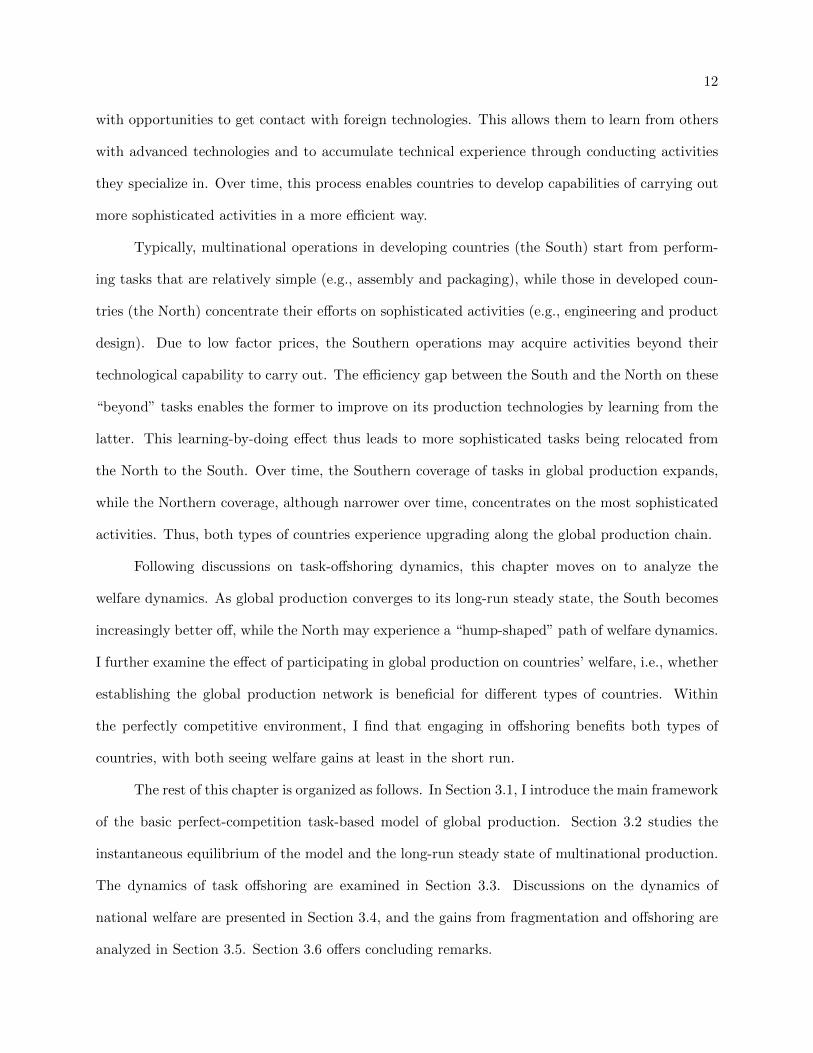
with opportunities to get contact with foreign technologies. This allows them to learn from others

with advanced technologies and to accumulate technical experience through conducting activities

they specialize in. Over time, this process enables countries to develop capabilities of carrying out

more sophisticated activities in a more efficient way.

Typically, multinational operations in developing countries (the South) start from perform-

ing tasks that are relatively simple (e.g., assembly and packaging), while those in developed coun-

tries (the North) concentrate their efforts on sophisticated activities (e.g., engineering and product

design). Due to low factor prices, the Southern operations may acquire activities beyond their

technological capability to carry out. The efficiency gap between the South and the North on these

“beyond” tasks enables the former to improve on its production technologies by learning from the

latter. This learning-by-doing effect thus leads to more sophisticated tasks being relocated from

the North to the South. Over time, the Southern coverage of tasks in global production expands,

while the Northern coverage, although narrower over time, concentrates on the most sophisticated

activities. Thus, both types of countries experience upgrading along the global production chain.

Following discussions on task-offshoring dynamics, this chapter moves on to analyze the

welfare dynamics. As global production converges to its long-run steady state, the South becomes

increasingly better off, while the North may experience a “hump-shaped” path of welfare dynamics.

I further examine the effect of participating in global production on countries’ welfare, i.e., whether

establishing the global production network is beneficial for different types of countries. Within

the perfectly competitive environment, I find that engaging in offshoring benefits both types of

countries, with both seeing welfare gains at least in the short run.

The rest of this chapter is organized as follows. In Section 3.1, I introduce the main framework

of the basic perfect-competition task-based model of global production. Section 3.2 studies the

instantaneous equilibrium of the model and the long-run steady state of multinational production.

The dynamics of task offshoring are examined in Section 3.3. Discussions on the dynamics of

national welfare are presented in Section 3.4, and the gains from fragmentation and offshoring are

analyzed in Section 3.5. Section 3.6 offers concluding remarks.

13

3.1 Set-up of the Model

Consider a world comprised of two countries: North (N) and South (S). There is one indus-

try supplying a final consumption product Y to both countries, with no trade or shipping cost.

Consumer preferences in the two countries are identical. The environment is perfectly competitive.

Labor is the sole factor of production, and it is inelastically supplied and immobile across countries.

The labor endowment of country i is denoted by Li, which is constant over time. Time is continuous

and indexed by t.

3.1.1 Production

The production of final good Y requires a continuum of tasks to be completed, indexed by

z ∈ [0, 1]. The value of z indicates the technological sophistication of tasks – a larger z indicates a

more sophisticated task. The production of Y at any time t is expressed as:

lnY (t) =

∫ 1

0lnx(z, t)dz, (3.1)

where x(z, t) is the amount of task z completed at time t. Each task can be carried out in either

country with constant returns to scale.

Consider the production technology. For any task z, there is a minimum unit labor require-

ment for completing it, which is given by

a(z) = ae−z, (3.2)

which is a time-invariant and non-increasing function of z.2

The North, on one side, has the most efficient technology for carrying out all tasks; i.e., it can

conduct any task using the minimum required amount of labor at any time. The South, on the other

side, possesses a stock of technologies initially at t = 0, but only those for low-sophistication tasks

are as good as their Northern corresponding ones. Specifically, the efficiency frontier of technology

in the South is denoted by T (t) at time t, with 0 < T (t) ≤ 1. At time t = 0, it is the case that

2 As in Young (1991), this assumption implies that the ultimate productivity of labor is non-decreasing in thetechnological sophistication of task production.

14

0 < T (0) < 1. For those simple tasks with z ≤ T (0), the South’s production technologies are as

efficient as the North’s. For the complicated ones with z > T (0), the Southern technologies are less

efficient, and the more sophisticated a task is, the further the South lags behind.3 Specifically,

the Southern unit labor requirement for conducting task z at t = 0 is given by

a(z, 0) =

a(z) = ae−z if z ≤ T (0) ,

aez−2T (0) if z > T (0) .

(3.3)

3.1.2 Learning-by-Doing

Any task can be conducted in either country. Therefore, offshoring happens out of the cost-

minimization incentive – the South conducts tasks offshored from the North, starting from the

relatively simple ones, while the North carries out the sophisticated ones. The two countries thus

form a multinational production chain. The South may obtain certain offshored tasks beyond

its technological efficiency frontier because of its low factor price. By conducting these “beyond”

tasks, the South observes the technological gap between the two countries and thus may accumulate

experience and improve its own technologies, thereby enhancing its production efficiency. This is

the learning-by-doing effect within the South. Furthermore, it is assumed that the learning-by-

doing effect is bounded with spillovers across tasks, with the minimum unit labor requirement

schedule serving as the learning boundary. Therefore, the South experiences reduction in its unit

labor requirement over time:

∂a(·, t)/∂ta(·, t)

= −∫ 1

02β

1

∣∣∣∣a(z, t)

a(z)> 1

LS(z, t) dz , (3.4)

where

1∣∣∣a(z,t)a(z) > 1

is an indicator function whose value equals 1 if the room for learning for task

z in the South is not exhausted at time t, and it equals 0 otherwise; LS(z, t) denotes the amount

of labor used for conducting task z in the South at time t; and β > 0 is a parameter that indicates

the learning ability of the South.4

3 The idea of technological distance has appeared in other models of learning. See, for example, Auerswald et al.(2000), Jovanovic and Nyarko (1996), and Mitchell (2000).

4 The environment is built upon Young (1991), where a general form of the bounded learning-by-doing functionis provided.

15

The learning function indicates first that the South is not able to learn from tasks that it is not

conducting. Secondly, for tasks that the South has already possessed the best technology, carrying

them out does not contribute to further efficiency improvement. Furthermore, the efficiency gain

from learning decreases in the Southern stock of advanced technology, as the situation a(z, t) = a(z)

becomes increasingly common when T (t) covers more tasks.

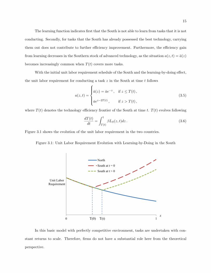
With the initial unit labor requirement schedule of the South and the learning-by-doing effect,

the unit labor requirement for conducting a task z in the South at time t follows

a(z, t) =

a(z) = ae−z , if z ≤ T (t) ,

aez−2T (t) , if z > T (t) ,

(3.5)

where T (t) denotes the technology efficiency frontier of the South at time t. T (t) evolves following

dT (t)

dt=

∫ 1

T (t)βLS(z, t)dz . (3.6)

Figure 3.1 shows the evolution of the unit labor requirement in the two countries.

Figure 3.1: Unit Labor Requirement Evolution with Learning-by-Doing in the South

0 1

Unit Labor Requirement

z

North

South at t = 0

South at t > 0

T(0) T(t)

In this basic model with perfectly competitive environment, tasks are undertaken with con-

stant returns to scale. Therefore, firms do not have a substantial role here from the theoretical

perspective.

16

3.2 Instantaneous Equilibrium and Steady State of Multinational Production

3.2.1 Instantaneous Equilibrium

Let wi(t) denote the wage rate in coutry i at time t. Then the unit cost functions for

conducting any task z in the two countries are, respectively,

CS(wS(t), z) = wS(t)a(z, t) , (3.7)

CN (wN (t), z) = wN (t)a(z) . (3.8)

As described earlier, a certain range of tasks are offshored to the South, and the offshoring starts

from the simplest tasks, since the South has the most advanced technologies for them since the

initial time. Thus, the cost conditions (3.7) and (3.8) combine to form a no-arbitrage condition in

task offshoring, indicating the pattern of task allocation between the two countries. There exists a

threshold task z(t) at time t such that CS(wS(t), z) = CN (wN (t), z) in equilibrium, i.e.,

wS(t) a(z(t), t) = wN (t) a(z(t)) , (3.9)

where z(t) is the most sophisticated task that is performed in the South. Thus, this threshold

task z(t) indicates the pattern of multinational production and countries’ respective position on

the global production chain – the South is at a “lower” position on the chain by carrying out tasks

with z ∈ [0, z(t)], while the North is at a “higher” position concentrating on the high-end tasks

with z ∈ (z(t), 1]. Certainly, one essential condition that enables offshoring is with regard to the

factor price: wS(t) ≤ wN (t). I will show that this condition is fully satisfied in later discussions.

The labor-market clearing conditions for the two countries at time t are given by

South :

∫ z(t)

0xS(z, t)a(z, t)dz = LS , (3.10)

North :

∫ 1

z(t)xN (z, t)a(z)dz = LN , (3.11)

where xi(z, t) denotes the amount of task z conducted in country i at time t.

With the task-based production function (3.1), each task receives the same share of the world

expenditure. The price of each task equals the minimum of its unit completion costs in the two

17

countries. Let E(t) denote the world expenditure on the final product Y at time t, defined as the

sum of factor payments in the two economies:

E(t) = wS(t)LS + wN (t)LN . (3.12)

Then the demand for a task z conducted in country i at time t is given by

xi(z, t) =E(t)

Ci(wi(t), z), i ∈ N,S . (3.13)

With the unit cost functions (3.7) and (3.8), along with (3.13), the labor-market clearing

conditions boil down to

South :

∫ z(t)

0

E(t)

wS(t)dz = LS , (3.10′)

North :

∫ 1

z(t)

E(t)

wN (t)dz = LN . (3.11′)

Therefore, the instantaneous equilibrium of the model at any time t is characterized by the

offshoring threshold determination condition (3.9), the labor-market clearing conditions (3.10′)

and (3.11′), and the world expenditure function (3.12). One equilibrium equation here can be

dropped by Walras’ Law, so that one variable can be chosen as numeraire. I thus normalize world

expenditure at unity: E(t) = 1, and hereby wage rates are measured as a share of the total world

factor income.

3.2.2 Steady State

From examining the instantaneous equilibrium conditions described above, it is found that

there exists a threshold task z∗ such that if it serves as the offshoring threshold under the equilibrium

conditions – all tasks with z ∈ [0, z∗] are offshored to the South, and all tasks with z ∈ (z∗, 1] are

conducted in the North, wage rates in the two countries are equalized. From conditions (3.10′) and

(3.11′), this wage-equalization task threshold z∗ is solved as

z∗ =LS

LS + LN. (3.14)

18

This task z∗ serves as the steady state of offshoring in this basic model.5 At the steady

state, the multinational production organization pattern is stable, with no more offshoring changes

happening. Other aspects of the economies, such as wage rates and production of the final good,

are also thus stabilized. Particularly, when multinational production arrives at the steady state,

all tasks are conducted using the most advanced technologies.

3.3 Transition Dynamics of Task Offshoring

Countries’ initial stocks of technology and their factor endowments determine their initial

positions on the global production chain, which then further determine their development there-

after. A relatively capable developing country may not see much space for learning thus efficiency

improvement by taking part in multinational production, while a factor-abundant country with

technologies lagging far behind may find great learning potential and opportunities. In this sec-

tion, I examine the transition dynamics of task offshoring under different circumstances, i.e., how

task-allocation across countries evolves over time with the learning-by-doing effect.

3.3.1 Transition Dynamics of Task Offshoring with an Initially Efficient South

In this situation, the South is relatively capable in terms of production technology initially:

T (0) ≥ z∗. Thus, it is easy to tell that all low-sophistication tasks below z∗ will be offshored

to the South, in order to fully exploit the cost advantages. All the offshored tasks thus may

be conducted using the best technologies. Given the unit labor requirement schedules and the

equilibrium conditions, the initial equilibrium is characterized by the following:

wS(0) ae−z(0) = wN (0) ae−z(0) , (3.15)∫ z(0)

0

1

wS(0)dz = LS , (3.16)∫ 1

z(0)

1

wN (0)dz = LN . (3.17)

5 From here on, all notations with the superscript “∗” stand for corresponding variables at the long-run steadystate.

19

These conditions indicate that at t = 0, the task offshoring threshold, z(0), and wage rates are

given by, respectively,

z(0) = z∗ =LS

LS + LN, (3.18)

wS(0) = wN (0) = w∗ =1

LS + LN. (3.19)

Therefore, for all the tasks offshored to the South, the country’s technology is as good as the North’s

– the South does not conduct anything that it is not good at. This implies that there is no learning

space for further improvement in the South. From the learning function (3.4), ∂a(·,t)/∂ta(·,t) = 0. As a

consequence, over time, the Southern unit labor requirement schedule keeps the same as that at

t = 0, and the Southern technology stock does not change over time (T (t) = T (0), ∀t). Given

that production efficiency stays unchanged in both countries, for all following time periods, the

equilibrium will also be the same as the initial one:

z(t) = z∗ =LS

LS + LN, ∀t (3.18′)

wS(t) = wN (t) = w∗ =1

LS + LN, ∀t. (3.19′)

Multinational production in this case thus arrives at its long-run steady state at the beginning.

Figure 3.2 displays this essentially static equilibrium situation in this case.

3.3.2 Transition Dynamics of Task Offshoring with Learning-by-Doing

In multinational production, most developing countries have enough labor resource but lack

advanced technologies. This situation may be modeled as T (0) < z∗. It is the main focus of this

basic model, and the task offshoring dynamics in this case are examined in this section.

Given that T (0) < z∗, z(0) ∈ (T (0), z∗) follows. The reasons are that an offshoring threshold

right at T (0) is not cost-minimizing and that without the best technologies for tasks beyond T (0),

it is costly to conduct all tasks [0, z∗] in the South in the initial time period. From (3.2), (3.3),

20

Figure 3.2: Dynamics of Task Offshoring: an Initially Efficient South (T (0) ≥ z∗)

0 1


z

North

South

T(t) = T(0)z(t) = z*

(3.9), (3.10′) and (3.11′), the initial equilibrium (t = 0) then is characterized by

wS(0) × aez(0)−2T (0) = wN (0) × ae−z(0) , (3.20)∫ z(0)

0

1

wS(0)dz = LS , (3.21)∫ 1

z(0)

1

wN (0)dz = LN . (3.22)

By examining the equilibrium conditions, the initial offshoring threshold, z(0), and wage rates are

found to be determined by the following conditions:

e2z(0)−2T (0) =1− z(0)

z(0)× LSLN

, (3.23)

wS(0) =z(0)

LS, (3.24)

wN (0) =1− z(0)

LN. (3.25)

At the equilibrium, with z(0) < z∗ = LSLS+LN

, it is the case that wS(0) < 1LS+LN

< wN (0). The

relatively low factor price in the South enables the offshoring to happen, ensuring that the simple

tasks for which the South has the best technologies may be offshored. Furthermore, except for

these simple tasks, the South also obtains tasks beyond its technological capability to carry out

(z(0) > T (0)). Figure 3.3 shows the initial equilibrium of this situation.

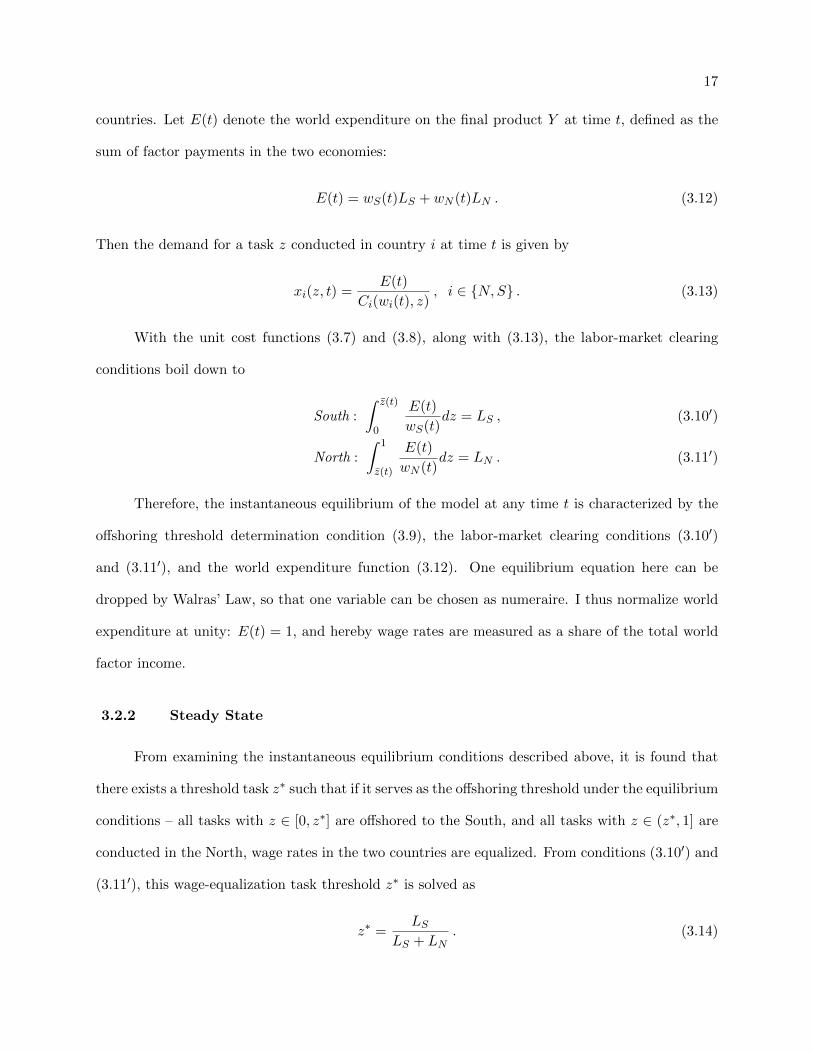
21

Figure 3.3: Initial Task Offshoring: an Initially Inefficient South (z∗ > T (0))

0 1


z

North

South at t=0

T(0) z(0) z*

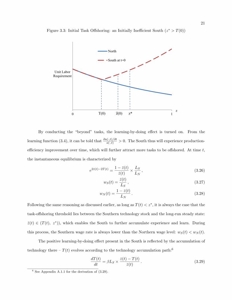
By conducting the “beyond” tasks, the learning-by-doing effect is turned on. From the

learning function (3.4), it can be told that ∂a(·,t)/∂ta(·,t) > 0. The South thus will experience production-

efficiency improvement over time, which will further attract more tasks to be offshored. At time t,

the instantaneous equilibrium is characterized by

e2z(t)−2T (t) =1− z(t)z(t)

× LSLN

, (3.26)

wS(t) =z(t)

LS, (3.27)

wN (t) =1− z(t)LN

. (3.28)

Following the same reasoning as discussed earlier, as long as T (t) < z∗, it is always the case that the

task-offshoring threshold lies between the Southern technology stock and the long-run steady state:

z(t) ∈ (T (t), z∗)), which enables the South to further accumulate experience and learn. During

this process, the Southern wage rate is always lower than the Northern wage level: wS(t) < wN (t).

The positive learning-by-doing effect present in the South is reflected by the accumulation of

technology there – T (t) evolves according to the technology accumulation path:6

dT (t)

dt= βLS ×

z(t)− T (t)

z(t). (3.29)

6 See Appendix A.1.1 for the derivation of (3.29).

22

The learning effect indicates that as long as the South conducts tasks beyond its current technology

stock, the country may always learn from what it does, i.e., dT (t)dt > 0 when z(t) > T (t).

The learning effect then further pushes the offshoring threshold toward more complicated

activities. The production efficiency improvement in the developing country makes more tasks, also

the relatively more sophisticated ones, be relocated there from the developed country. Therefore,

the South climbs up the global value chain by expanding its task scope and doing increasingly

sophisticated tasks as well. This can be seen by examining (3.26):

dz(t)

dt=

2z(t) (1− z(t))1 + 2z(t) (1− z(t))

× dT (t)

dt, (3.30)

which further implies that

0 <dz(t)

dt<dT (t)

dt, (3.31)

during the process of Southern learning (i.e., dT (t)dt > 0). At the same time, by increasingly offshoring

tasks to the South, the North more and more focuses on the most difficult activities. Although the

range of tasks that are performed in the North narrows over time, the average task sophistication

increases. Therefore, the developed country also moves up the global value chain in this sense.

Moving up the multinational value chain is thus given a specific definition as an upgrading in the

set of tasks that a country conducts.

Then the question comes to how strong the learning effect is and whether it diminishes

over time. From (3.29), the learning space on “beyond” tasks – the distance between z(t) and T (t)

relative to the whole range of offshored tasks z(t) – largely determines the strength of learning effect.

As time passes, the speed of technology accumulation exceeds the speed of offshoring expansion (i.e,

dT (t)dt > dz(t)

dt > 0), and thus the learning opportunities will be gradually exhausted. This indicates

that the offshoring threshold, as well as the technology stock in the South, will evolve over time

following a concaved-shaped path:7

d2T (t)

dt2< 0, and

d2z(t)

dt2< 0 . (3.32)

7 See Appendix A.1.1 and Appendix A.1.2 for the derivation.

23

In the long run, the offshoring threshold, z(t), and the Southern technology stock, T (t),

converge to the same steady state z∗.8 Therefore, for all tasks that are offshored to the South,

the country will be having the best technologies for them in the long run. All the tasks, no matter

conducted in which country, will then be carried out with the best technologies available. Figure 3.4

shows the convergence paths for both the Southern technology stock T (t) and the task offshoring

threshold z(t).

Figure 3.4: Dynamics of Task Offshoring: an Initially Inefficient South (z∗ > T (0))

0

z(t)

T(t)

t

z*

3.4 Dynamics of National Welfare and Gains from Offshoring

In this section, two important questions are examined: (1) during the process of offshoring

evolution, how will the countries’ welfare change over time? and (2) do countries gain from pro-

duction fragmentation and offshoring? For both questions, answers under the first situation – the

static equilibrium with a sufficiently efficient South – can be easily understood once the dynamics

under the second case are illustrated. Therefore, I will mainly focus on the dynamic case here.

8 Given (3.26), (3.29) and (3.30), together with the value of z∗ shown in (3.14), it is easy to verify that when

z(t) = z∗, both dT (t)dt

and dz(t)dt

decrease to 0.

24

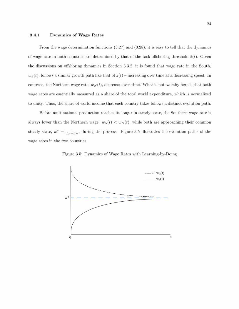
3.4.1 Dynamics of Wage Rates

From the wage determination functions (3.27) and (3.28), it is easy to tell that the dynamics

of wage rate in both countries are determined by that of the task offshoring threshold z(t). Given

the discussions on offshoring dynamics in Section 3.3.2, it is found that wage rate in the South,

wS(t), follows a similar growth path like that of z(t) – increasing over time at a decreasing speed. In

contrast, the Northern wage rate, wN (t), decreases over time. What is noteworthy here is that both

wage rates are essentially measured as a share of the total world expenditure, which is normalized

to unity. Thus, the share of world income that each country takes follows a distinct evolution path.

Before multinational production reaches its long-run steady state, the Southern wage rate is

always lower than the Northern wage: wS(t) < wN (t), while both are approaching their common

steady state, w∗ = 1LS+LN

, during the process. Figure 3.5 illustrates the evolution paths of the

wage rates in the two countries.

Figure 3.5: Dynamics of Wage Rates with Learning-by-Doing

0 t

w*

wN(t)

wS(t)

25

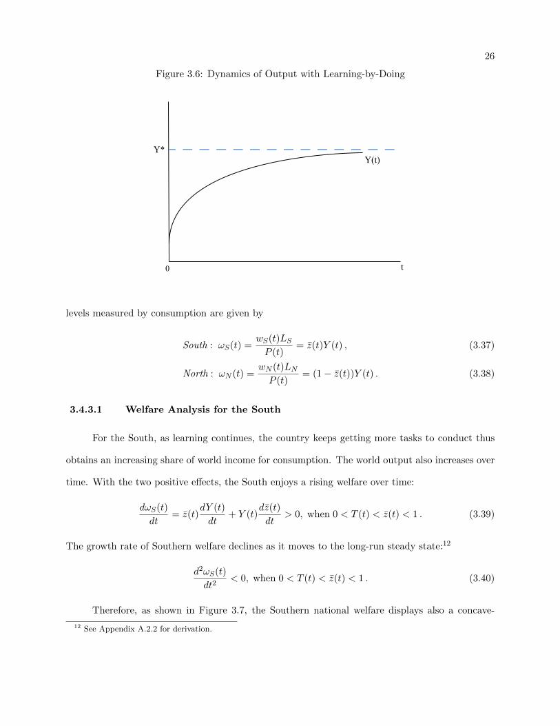
3.4.2 Dynamics of Output

As offshoring evolves, at any point of time t, the world output amount of the consumer

product is9

Y (t) =LN

a(1− z(t))× ez(t)2−T (t)2 × e

12 . (3.33)

Examining the output function, it is found that the world output displays also a concave-shaped

growth path over time:10

dY (t)

dt= Y (t)× 2[z(t)− T (t)]

dT (t)

dt> 0, when 0 < T (t) < z(t) < 1, (3.34)

d2Y (t)

dt2< 0, when 0 < T (t) < z(t) < 1 . (3.35)

Therefore, when more and more tasks are reallocated from the North to the South, the total world

output grows over time. While the learning space is increasingly exhausted during the process,

the growth rate of output declines gradually. In the long run, the output amount converges to its

steady state:11

Y ∗ =

(LS + LN

a

)e

12 . (3.36)

Figure 3.6 shows the growth pattern of output over time.

3.4.3 Dynamics of National Welfare

As discussed in Section 3.4.2, the world output increases over time. As a whole, the world

gains as the total consumption level increases. At the same time, wage rates in the two countries

show different evolution patterns – the South experiences a positive-sloping path, while the Northern

share of world income shrinks. Hence, the question arises as to whether the two countries’ respective

welfare grows as the learning process continues. Assuming no trade or shipping cost, within the

perfectly competitive environment, the consumer price of the final product is the same across

countries. The price index of the final good at time t is P (t) = 1Y (t) . Then the countries’ welfare

9 See Appendix A.2.1 for the derivation.10 See Apeendix A.2.1 for the derivation.11 It is easy to obtain the steady state of output with (3.14) and the output expression (3.33).

26

Figure 3.6: Dynamics of Output with Learning-by-Doing

0 t

Y*Y(t)

levels measured by consumption are given by

South : ωS(t) =wS(t)LSP (t)

= z(t)Y (t) , (3.37)

North : ωN (t) =wN (t)LNP (t)

= (1− z(t))Y (t) . (3.38)

3.4.3.1 Welfare Analysis for the South

For the South, as learning continues, the country keeps getting more tasks to conduct thus

obtains an increasing share of world income for consumption. The world output also increases over

time. With the two positive effects, the South enjoys a rising welfare over time:

dωS(t)

dt= z(t)

dY (t)

dt+ Y (t)

dz(t)

dt> 0, when 0 < T (t) < z(t) < 1 . (3.39)

The growth rate of Southern welfare declines as it moves to the long-run steady state:12

d2ωS(t)

dt2< 0, when 0 < T (t) < z(t) < 1 . (3.40)

Therefore, as shown in Figure 3.7, the Southern national welfare displays also a concave-

12 See Appendix A.2.2 for derivation.

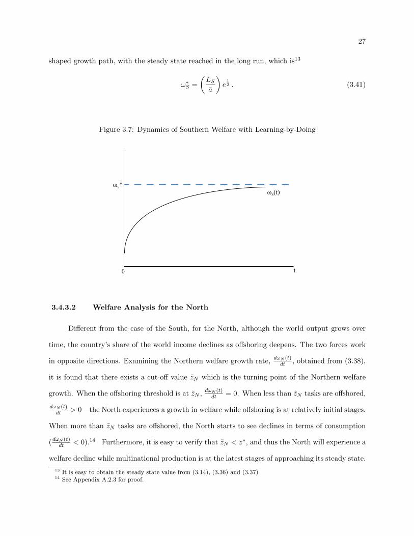
27

shaped growth path, with the steady state reached in the long run, which is13

ω∗S =

(LSa

)e

12 . (3.41)

Figure 3.7: Dynamics of Southern Welfare with Learning-by-Doing

0 t

ωS*ωS(t)

3.4.3.2 Welfare Analysis for the North

Different from the case of the South, for the North, although the world output grows over

time, the country’s share of the world income declines as offshoring deepens. The two forces work

in opposite directions. Examining the Northern welfare growth rate, dωN (t)dt , obtained from (3.38),

it is found that there exists a cut-off value zN which is the turning point of the Northern welfare

growth. When the offshoring threshold is at zN , dωN (t)dt = 0. When less than zN tasks are offshored,

dωN (t)dt > 0 – the North experiences a growth in welfare while offshoring is at relatively initial stages.

When more than zN tasks are offshored, the North starts to see declines in terms of consumption

(dωN (t)dt < 0).14 Furthermore, it is easy to verify that zN < z∗, and thus the North will experience a

welfare decline while multinational production is at the latest stages of approaching its steady state.

13 It is easy to obtain the steady state value from (3.14), (3.36) and (3.37)14 See Appendix A.2.3 for proof.

28

Intuitively, when close to the steady state, the learning space is almost exhausted – the negative

income-share effect thus outweighs the positive productivity effect stemming from learning. At the

steady state, the Northern long-run welfare is

ω∗N =

(LNa

)e

12 . (3.42)

Comparing the long-run with the initial state of Northern welfare, ω∗N and ωN (0), it is found that

ω∗NωN (0)

= eT (0)2−z(0)2< 1 , (3.43)

which indicates that the long-run steady-state welfare of the North will actually be lower than its

initial state when it just starts offshoring. How big the gap is depends on the initial learning space

in the host country. Therefore, in sum, the evolution path of Northern welfare essentially depends

on the two countries’ relative endowments and the initial technology stocks.

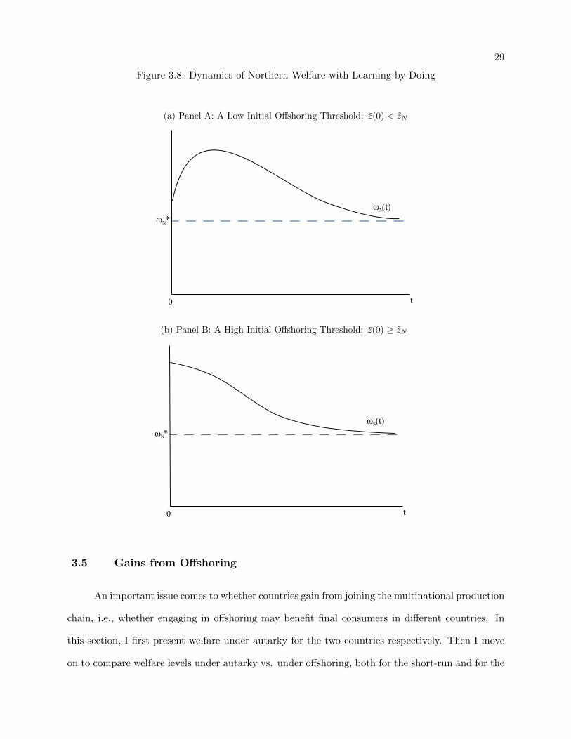
Figure 3.8 illustrates two possible cases of Northern welfare evolution. In Panel A, the initial

offshoring threshold z(0) < zN . The North thus experiences welfare growth first while the efficiency

gain brought by Southern learning outweighs the income effect. The situation will reverse later after

more than zN tasks are offshored. This case is more likely to happen when the South is adequately

abundant in labor (a large LS thus a high zN ) and/or has a low technology stock initially (a low

T (0) thus a low z(0)). In Panel B, more than zN tasks are offshored at the beginning. Over time,

the North sees declining welfare until it reaches the steady state. This is more likely the case if the

South has a small labor force and/or possesses relatively high stock of technology initially. From

the short-run perspective of the North, it may be beneficial to form the multinational production

chain when the host country is large and/or lagging far behind in terms of production efficiency, so

that the North can enjoy welfare growth at least in the short run. In contrast, from the long-run

perspective, it may be better if the South is a “balanced” economy – the technology stock and the

factor endowment are balanced, so that the initial offshoring threshold does not deviate too much

from the technology stock in the host country.

29

Figure 3.8: Dynamics of Northern Welfare with Learning-by-Doing

(a) Panel A: A Low Initial Offshoring Threshold: z(0) < zN

0 t

ωN*ωN (t)

(b) Panel B: A High Initial Offshoring Threshold: z(0) ≥ zN

0 t

ωN*ωN (t)

3.5 Gains from Offshoring

An important issue comes to whether countries gain from joining the multinational production

chain, i.e., whether engaging in offshoring may benefit final consumers in different countries. In

this section, I first present welfare under autarky for the two countries respectively. Then I move

on to compare welfare levels under autarky vs. under offshoring, both for the short-run and for the

30

long-run, which leads to the discussions on gains from offshoring. As mentioned earlier, the static

case of offshoring can essentially be viewed as a sub-case of the dynamic situation. Therefore, in

this section, the main discussions are on the dynamic situation with a positive learning effect.

3.5.1 Welfare under Autarky

Under autarky, both countries have to conduct all tasks to produce the final product according

to (3.1). They start with the same situation as t = 0 under offshoring – the productivity schedules

are given by (3.2) and (3.3), for the North and South, respectively. Without offshoring, countries are

not able to get touch with foreign technologies, which indicates that there is no learning opportunity

for the South. Therefore, the two economies will stay the same as where they start initially – the

time index t can thus be omitted for the autarky case.15

With full employment, the amount of task z conducted in a country can be expressed as

South : xAS (z) =LS

a(z, t), (3.44)

North : xAN (z) =LNa(z)

. (3.45)

This further indicates that the final output level, which is also the real consumption thus implies

a country’s welfare under autarky, is given by16

South : ωAS = Y AS =

LSa× e−[T (0)−1]2+ 1

2 , (3.46)

North : ωAN = Y AN =

LNa× e

12 . (3.47)

3.5.2 Gains from Offshoring with Learning-by-Doing

Given the autarky welfare levels, in this section, I discuss the gains from offshoring with the

learning-by-doing effect turned on. With learning, the economies evolve over time – the welfare

discussions will include both short-run and long-run analyses, i.e., whether countries gain when

15 The time index will be omitted hereby in this subsection, and the superscript “A” indicates the correspondingvariables under autarky.

16 The equations are easy to obtain given the production function (3.1) and the task amount expressions (3.44)and (3.45).

31

they just start participating in offshoring and whether they gain when they reach the steady state

in the long run.

Initial Gains Comparing the autarky case and the offshoring-with-learning case, it is

found that offshoring brings both countries higher welfare levels initially when they just open to

form the multinational production chain:17

ωS(0)

ωAS= e(z(0)−1)2

> 1 , and (3.48)

ωN (0)

ωAN= ez(0)2−T (0)2

> 1 . (3.49)

This result shows that in the short run, offshoring is beneficial for both countries with advanced

technologies and those lagging behind. Under multinational production, countries gain initially

from specializing in distinct sets of activities. However, the initial gains may be unbalanced between

countries – a large South, thus a high task offshoring threshold z(0), brings more welfare gains to

the North, than a small South, while a small South will self-benefit more.

Gains in the Long Run As discussed in Section 3.4, the South experiences continuous

welfare improvement when offshoring evolves over time. Therefore, it is easy to see that when t > 0,

the South is always better off than under autarky when multinational production progresses. In

the long run, it is the case that

ω∗SωAS

= e(T (0)−1)2> 1 (3.50)

For the North, it has been seen that its national welfare may show different possible paths

of evolution. Comparing the autarky welfare vs. the welfare under offshoring, it is found that

ωN (t) > ωAN before the economy reaches the steady state.18 In the long run, ω∗N = ωAN . Hence,

the consumers in the North are also better off under multinational production during the evolution

process. In sum, with the Southern learning effect, both the technologically advanced and less

advanced countries may gain. While the short-run gain is positive for both, the long-run gain at

17 The countries’ initial welfare levels under offshoring are from (3.37) and (3.38), together with (3.33), while t = 0.The comparison results are then easily obtained by comparing the welfare levels under offshoring vs. under autarky,with condition (3.23) applied.

18 ωN (t)

ωAN

= ez(t)2−T (t)2 > 1 before arriving at steady state.

32

the steady state is mainly for the South.

3.6 Concluding Remarks

A task-based model of multinational production dynamics with learning-by-doing is capable

of accounting for the evidences that both the developed and developing economies experience task

upgrading over time. To a certain extent, this basic perfect-competition story coincides with the

industrialization and growth experience of many countries. The model shows that host countries,

although lagging behind in terms of production efficiency, obtain an increasingly wide range of

relatively sophisticated activities to carry out over time. They also see increases in their share of

world income and consumption. This suggests the progress of foreign-direct-investment-led indus-

trialization observed in many countries. For the developed countries, they increasingly concentrate

efforts on the most complicated activities, as also seen in the real world.

The dynamics of welfare in this model show that taking part in multinational production is

favorable for both types of participants. Both countries are better off than under autarky since the

very beginning when they are engaged in offshoring. This situation continues during the evolution

process. In the long run, the South definitely enjoys a better welfare at the steady state than the

autarky case, while the North is at least as well off as its autarky level. Therefore, both countries

benefit from opening to offshoring.

Certainly, the perfect-competition framework discussed in this chapter provides a convenient

environment for analysis, while it leaves out certain factors such as the consideration of final

product’s varieties. In later chapters, the model under different frameworks will be examined and

thus provide additional insights into the dynamics of global value chain.

Chapter 4

The Dynamics of Global Value Chain in Monopolistic Competition

This chapter provides a theory of global value chain dynamics in the monopolistic competition

framework. In the model, there is one industry supplying a differentiated final consumer product.

Within the industry, there is a continuum of multinational firms, with each producing a single

and distinct variety and selling it in both countries. The multinational firms have subsidiaries in

both the developed and developing countries, with subsidiaries in different countries specializing in

different sets of activities.

Similar like in Chapter 3, the model is task-based, with the technology for producing a final

good modeled as a spectrum of production “tasks” that are ranked according to their degree of

technological sophistication. This spectrum serves as the basis for global production and value chain

analyses, and moving up the global value chain is then given a specific definition as an upgrading

in the set of tasks that a country, an industry, or a subsidiary specializes in. For different countries

and firms, the task-upgrading pattern may vary.

In the model, the learning-by-doing effect is the main driving force of multinational produc-

tion evolution. Subsidiaries in developing countries may receive tasks on which they lag behind

in terms of technology. By conducting these tasks, the subsidiaries engage in contact with foreign

advanced technologies, and further exploration and actualization of those technologies empower

efficiency improvement in these subsidiaries over time.

This chapter examines the dynamic welfare effects of participating in global production. As

global production converges to the steady state, the South experiences welfare gains constantly

34

along the way. The North, in contrast, may see a long-run welfare level possibly lower than some

intermediate level of offshoring. Compared with autarky, the North enjoys positive gains since

the initial time when offshoring starts, and it is also better off in the long run, if the steady-state

offshoring threshold is within the range of offshorable tasks. The effect of offshoring turns out to

be different for the country with technological disadvantages. Engaging in offshoring may have a

negative effect for the South initially, wherein the short-term involves pains, but the effect dissipates

later while offshoring continues bringing welfare benefits to the country over time. In the long run,

the effect is always positive – the South is always better off at the steady state than it is under

autarky. Thus, both countries may benefit from joining in global production, but the paths differ.

Different effects contribute to the welfare dynamics. The South and North experience a

factor reward increase and decrease, respectively, when global production evolves. At the same

time, consumers in both countries enjoy an increasing number of consumption options on the

market – the number of varieties available keeps growing along the way. The output dynamics

of each variety also contributes to the welfare changes over time. These effects are analyzed and

discussed specifically in the chapter.

This chapter is organized as follows. In Section 4.1, I introduce the theoretical environment.

Section 4.2 studies the instantaneous equilibrium and the steady state situation in the long run.

In Section 4.3, I examine the evolution dynamics of task offshoring under different circumstances.

This section also includes discussions of the dynamics of other important economic aspects, such

as product variety and national welfare. Section 4.4 discusses the gains from fragmentation and

offshoring by comparing national welfare in the state of global production to the state under autarky.

Section 4.5 lists the major conclusions.


Consider a world comprised of two countries: North (N) and South (S). There is an industry

supplying a differentiated final consumer product, in which there is a continuum of firms, each

producing a single and distinct variety indexed by j and selling it in both countries. Firms are

35

symmetric – the final varieties are only different in the sense that they are under different brand

names. Labor is the sole factor of production, and it is inelastically supplied and immobile across

countries. The labor endowment of country i is denoted by Li, which is constant over time. Time

is continuous and is indexed by t.

4.1.1 Preference

Consumer preferences are assumed to be identical in the two countries, and the instantaneous

preference of a representative consumer at any time t is given by a C.E.S. utility function:

U(t) =

[∫ J(t)

0q(j, t)ρdj

] 1ρ

, (4.1)

where J(t) denotes the number of product varieties available and thus also the number of firms at

time t; q(j, t) is the consumption of good j at time t; and 0 < ρ < 1.

This instantaneous utility function implies that the elasticity of substitution between any two

varieties within this industry is constant and equals σ = 11−ρ > 1. As in Dixit and Stiglitz (1977),

the demand for brand j at time t is given by

q(j, t) =E(t)p(j, t)−σ

P (t)1−σ , (4.2)

where E(t) stands for the aggregate consumer expenditure at time t; p(j, t) denotes the price of

brand j at time t; and P (t) is a price index such that

P (t) =

[∫ J(t)

0p(j, t)1−σdj

] 11−σ

. (4.3)

4.1.2 Product Market

Facing the constant elasticity demand function derived above, firms choose the same profit

maximization markup equal to 1ρ . Given the symmetry of firms, the pricing rule is thus given by

p(j, t) = p(t) =c(j, t)

ρ=c(t)

ρ, (4.4)

where c(t) is the marginal cost of producing any variety j at time t. Assuming no trade or trans-

portation cost, the price of any product is the same across countries.

36

Firms need to pay a fixed cost during each time period. The fixed cost f > 0 is the amount

of Northern labor used. It can be viewed as the labor effort needed for conducting the necessary

non-offshorable activities. The fixed cost is the same for all firms. This yields the firm profit:

π(j, t) = π(t) =E(t)

σ

(c(t)

ρP (t)

)1−σ− wN (t)f , (4.5)

where wN (t) is the wage level in the North at time t, and E(t) could be expressed as

E(t) =

∫ J(t)

0p(j, t)q(j, t)dj . (4.6)

4.1.3 Production

The production of any variety requires the completion of an identical continuum of tasks,

indexed by z ∈ [0, 1]. The numeric value of z measures the technological sophistication of a task –

the larger z is, the more sophisticated the task is. The production technology is identical across all

varieties. Given the symmetry of firms, at time t, the production function for any variety j is

lnY (j, t) = lnY (t) =

∫ 1

0lnx(j, z, t)dz , (4.7)

where x(j, z, t) is the amount of task z that is completed at time t for producing good j. Each task

can be located and carried out in either country.

Consider the production technology. For any task z, there is a minimum unit labor require-

ment, given by

a(z) = ae−z , (4.8)

where a is a positive constant. It is time invariant and non-increasing in z.

The North masters the most advanced technologies for all tasks. Thus, the Northern plants

can perform any task using the minimum amount of labor indicated by a(z). In contrast, the

Southern plants lag behind technologically – they only possess the most efficient technology for

a range of low-sophistication tasks, and the situation is identical for all varieties’ production.

Specifically, initially at t = 0, the stock of technologies in the South is denoted by T (0), with

0 < T (0) < 1. For the relatively simple tasks with z ≤ T (0), the South is as efficient as the

37

North in carrying out these tasks. For the tasks that are relatively difficult to carry out (with

z > T (0)), the South does not have the best technologies initially; and the more sophisticated a

task is, the further the South lags behind the North in terms of production technology. Specifically,

the Southern subsidiaries’ unit labor requirement schedule at t = 0 is given by1

a(z, 0) =

a(z) = ae−z , if z ≤ T (0),

aez−2T (0) , if z > T (0).

(4.9)


Tasks can be completed in the South or in the North. Firms are multinational enterprises

in the sense that they have subsidiaries in both countries, performing different sets of tasks. For

the South, certain tasks beyond its technological capability may be offshored to the country, which

enables subsidiaries there to observe the technological gap between themselves and their North-

ern counterparts. By conducting these “beyond” tasks, the Southern plants can thus accumulate

experience and improve their own technologies, thereby enhancing production efficiency. This is

the effect of learning-by-doing in the South. Moreover, the learning-by-doing effect is assumed

to be bounded and with spillovers across tasks, with the North serving as the technology fron-

tier and learning boundary. Therefore, the Southern plants experience reduction in the unit labor

requirement over time:2

∂a(·, t)/∂ta(·, t)

= −∫ 1

02β

1

∣∣∣∣a(z, t)

a(z)> 1

LS(j, z, t) dz , (4.10)

where

1∣∣∣a(z,t)a(z) > 1

is an indicator function that equals 1 if the learning room for task z in the

South is not exhausted at time t; LS(j, z, t) denotes the amount of labor used for conducting task

z in the Southern subsidiary of brand j at time t; and β > 0 is a parameter that measures the

learning ability of the South.

1 Given the symmetry of firms, subsidiaries in the same country have the same technologies, and thus the unitlabor requirement schedules do not depend on the variety argument j.

2 The environment here is built upon Young (1991), in which a general functional form of bounded learning-by-doing is provided.

38

On one hand, the function of learning-by-doing indicates that the Southern plants are not

able to learn from the tasks that they do not conduct. On the other hand, for tasks on which

learning space has already been exhausted (a(z, t) = a(z)), carrying them out does not contribute

to further efficiency improvement. The learning effect is positive only if the Southern plants perform

tasks for which they have not obtained the best techniques.

With the South’s initial unit labor requirement schedule and the learning-by-doing effect, the

unit labor requirement for completing a task z in the South at time t follows

a(z, t) =

a(z) = ae−z , if z ≤ T (t) ,

aez−2T (t) , if z > T (t) ,

(4.11)

where T (t) refers to the technology stock in the South at time t. T (t) evolves according to

dT (t)

dt=

∫ 1

T (t)βLS(j, z, t)dz . (4.12)

Figure 4.1 shows the evolution of the unit labor requirement schedule in the South.

Figure 4.1: Unit Labor Requirement Evolution with Learning-by-Doing in the South

0 1


z

North

South at t = 0

South at t > 0

T(0) T(t)

A task can be conducted by subsidiaries in the North or in the South, using the corresponding

technology indicated by function (4.8) or (4.11), depending on the offshoring pattern prevailing at

39

the time. Each brand establishes only one subsidiary in a country, which completes all tasks

allocated to that country by its own brand. There is free entry in the market at all times. The new

entrants bring in new distinct brands/varieties, which use the same set of tasks and the identical

production function as all already-existing players do. Hence, when a new firm enters the market,

it will also use the same offshoring pattern as for the current firms. Free entry draws firms’ profit

to zero, which then determines the number of varieties present on the market.

4.2 Instantaneous Equilibrium and Steady State of Multinational Production


Let wi(t) denote the wage rate prevailing in country i at time t. Then given the symmetry of

firms, the cost functions for conducting task z for any brand j in the two countries are, respectively,

CS(wS(t), j, z) = wS(t)a(z, t) , (4.13)

CN (wN (t), j, z) = wN (t)a(z) , (4.14)

Under offshoring, certain tasks are allocated to the South. As described earlier, for the range

of low-sophistication tasks with z ≤ T (t), the Southern plants are as competent in conducting them

as their Northern counterparts. However, for the high-end tasks, the South increasingly lags behind.

Thus, with consideration of production efficiency, the firms initially offshore relatively simple tasks,

with their Southern subsidiaries conducting low-end tasks while the Northern subsidiaries focus on

relatively sophisticated activities. Specifically, the cost functions (4.13) and (4.14) combine to form

a no-arbitrage condition in task offshoring, indicating the pattern of task allocation between the two

countries. There exists a threshold task z(t) at time t such that CN (wN (t), j, z) = CS(wS(t), j, z);

or equivalently,

wN (t) a(z(t)) = wS(t) a(z(t), t) , (4.15)

with z(t) denoting the most sophisticated task that is conducted in the Southern plants.3 Thus,

for all firms within the industry, tasks with z ∈ [0, z(t)] are allocated to the South, and tasks with

3 z(t) is the same across all plants because firms are symmetric.

40

z ∈ (z(t), 1] are performed in the North. Given that the value chain of the industry is represented

by the whole spectrum of tasks that can be disintegrated and spread over national borders, with

each task adding value to the final industrial product, the pattern of task-allocation across countries

implied by condition (4.15) indicates countries’ respective position on the global value chain – the

South is lower than the North. This condition also implies that all firms incur the same marginal

cost of production and thus have the same pricing behavior at all times. Certainly, an essential

condition that enables offshoring is wS(t) ≤ wN (t), so that the South has the unit cost advantages

in performing those low-end activities. It will be shown later that this condition is always satisfied.

The labor market clearing conditions for the two countries at time t are given by

South :

∫ z(t)

0xS(z, t)a(z, t)dz = LS , (4.16)

North :

∫ 1

z(t)xN (z, t)a(z)dz + J(t)f = LN , (4.17)

where f is the fixed labor cost incurred by every firm in each time period; J(t) is the number of

varieties at time t; and xi(z, t) denotes the total amount of task z conducted by all subsidiaries in

country i at time t.

Let E(t) denote the total world expenditure on final products at time t. I0-t is equal to the

sum of factor payments in the two countries:

E(t) = wS(t)LS + wN (t)LN . (4.18)

Given the pricing rule, the demand for a task z conducted in country i at time t is given by

xi(z, t) =ρE(t)

Ci(wi(t), z), i ∈ N,S , (4.19)

where Ci(wi(t), z) is the same across firms.

With the unit cost functions (4.13) and (4.14), along with (4.19), the labor market clearing

conditions become

South :

∫ z(t)

0

ρE(t)

wS(t)dz = LS , (4.16′)

North :

∫ 1

z(t)

ρE(t)

wN (t)dz + J(t)f = LN . (4.17′)

41

The free-entry condition drives the firms’ profit to zero. Given the symmetry of firms, the

zero-profit condition can be simplified to4

E(t)

σJ(t)= wN (t)f . (4.20)

Thus, the instantaneous aggregate equilibrium of the model at any time t is characterized

by the offshoring threshold determination condition (4.15), the labor market clearing conditions

(4.16′) and (4.17′), the world expenditure function (4.18), and the zero-profit condition (4.20). One

equilibrium equation here can be dropped by Walras’ law, so that one variable can be chosen as the

numeraire. I thus normalize the world expenditure at unity, with E(t) = 1. Hence, all the wages

are measured as shares of the world’s total factor income.

4.2.2 Steady State

At the steady state, the task-allocation pattern of global production stays stable. No more

tasks are reallocated from one country to the other. Other aspects of the two economies, such as

wage rates and the South’s technology stock, are also stabilized. By examining the labor market

clearing conditions (4.16′) and (4.17′), along with the zero-profit condition (4.20), it is found that

there exists a threshold task z∗ such that if all tasks with z ∈ [0, z∗] are offshored to the South

and all tasks with z ∈ (z∗, 1] are retained in the North, the wage rates of the two countries are

equalized. Specifically, the time-invariant z∗ is solved to be

z∗ =LS

ρ (LS + LN ). (4.21)

z∗ serves as the threshold task of offshoring at the steady state if it is within the range of

offshorable tasks ( LSρ (LS+LN ) ≤ 1).5 If z∗ exceeds the range of offshorable tasks, then offshoring

will stop when all offshorable tasks have been allocated to the South and the North focuses solely

on non-offshorable activities. In this circumstance, the task threshold of offshoring will be z∗′ = 1

4 It is straightforward to obtain (4.20) from examining the profit function (4.5), with considering the aggregateprice index expression (4.3) and the pricing rule specified by (4.4).

5 This condition is more likely to be satisfied if in consumers’ eyes, the degree of substitutability among varietiesis relatively high.

42

at steady state. Therefore, the extent of substitutability among varieties in this industry largely

determines where the offshoring threshold will be at steady state. Certainly, with learning being

the main driving force of technical improvement, if both countries are involved in conducting the

offshorable tasks in the long run, the South will be as capable as the North on the tasks it conducts

when the steady state is achieved. The unit completion cost of the threshold task of offshoring at

the steady state is thus the same in the two countries. The steady state of global production is then

featured with equalized wage rates and all tasks being carried out using the best technologies.6

4.3 Transition Dynamics

Countries’ initial stocks of technology and their factor endowments determine their initial

positions on the global value chain, which further indicate the learning opportunities in the global

environment. As discussed earlier in the chapter, if a Southern subsidiary conducts tasks at which

it is not particularly competent, the learning effect will be positive in the sense that the production

efficiency on sophisticated tasks will be improved, through exploring advanced technologies while

carrying out the tasks. In contrast, by conducting tasks for which the best technologies have already

been in use, plants are not able to obtain further learning opportunities. Therefore, countries’ initial

positions on the global value chain are important for understanding the transitional dynamics. In

this section, I examine the transition dynamics of the model – the movement from an initial situation

of task-allocation to the steady state of global production.

Depending upon how far the South lags behind in terms of technology (essentially, where

T (0) is) and where the steady state is, there are four possible cases with regard to how global

production may evolve over time:

Case I. Normal Evolution This is the situation where the steady state stays within the range

of offshorable tasks (0 < z∗ ≤ 1) and the initial stock of technology in the South is not adequate for

efficiently performing all tasks that could be offshored to the country at the steady state (T (0) < z∗).

6 From here on, all notations with the superscript “∗” stand for corresponding variables at the long-run steadystate.

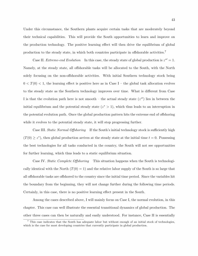
43

Under this circumstance, the Southern plants acquire certain tasks that are moderately beyond

their technical capabilities. This will provide the South opportunities to learn and improve on

the production technology. The positive learning effect will then drive the equilibrium of global

production to the steady state, in which both countries participate in offshorable activities.7

Case II. Extreme-end Evolution In this case, the steady state of global production is z∗′ = 1.

Namely, at the steady state, all offshorable tasks will be allocated to the South, with the North

solely focusing on the non-offshorable activities. With initial Southern technology stock being

0 < T (0) < 1, the learning effect is positive here as in Case I – the global task allocation evolves

to the steady state as the Southern technology improves over time. What is different from Case

I is that the evolution path here is not smooth – the actual steady state (z∗′) lies in between the

initial equilibrium and the potential steady state (z∗ > 1), which thus leads to an interruption in

the potential evolution path. Once the global production pattern hits the extreme end of offshoring

while it evolves to the potential steady state, it will stop progressing further.

Case III. Static Normal Offshoring If the South’s initial technology stock is sufficiently high

(T (0) ≥ z∗), then global production arrives at the steady state at the initial time t = 0. Possessing

the best technologies for all tasks conducted in the country, the South will not see opportunities

for further learning, which thus leads to a static equilibrium situation.

Case IV. Static Complete Offshoring This situation happens when the South is technologi-

cally identical with the North (T (0) = 1) and the relative labor supply of the South is so large that

all offshorable tasks are offshored to the country since the initial time period. Since the variables hit

the boundary from the beginning, they will not change further during the following time periods.

Certainly, in this case, there is no positive learning effect present in the South.

Among the cases described above, I will mainly focus on Case I, the normal evolution, in this

chapter. This case can well illustrate the essential transitional dynamics of global production. The

other three cases can then be naturally and easily understood. For instance, Case II is essentially

7 This case indicates that the South has adequate labor but without enough of an initial stock of technologies,which is the case for most developing countries that currently participate in global production.

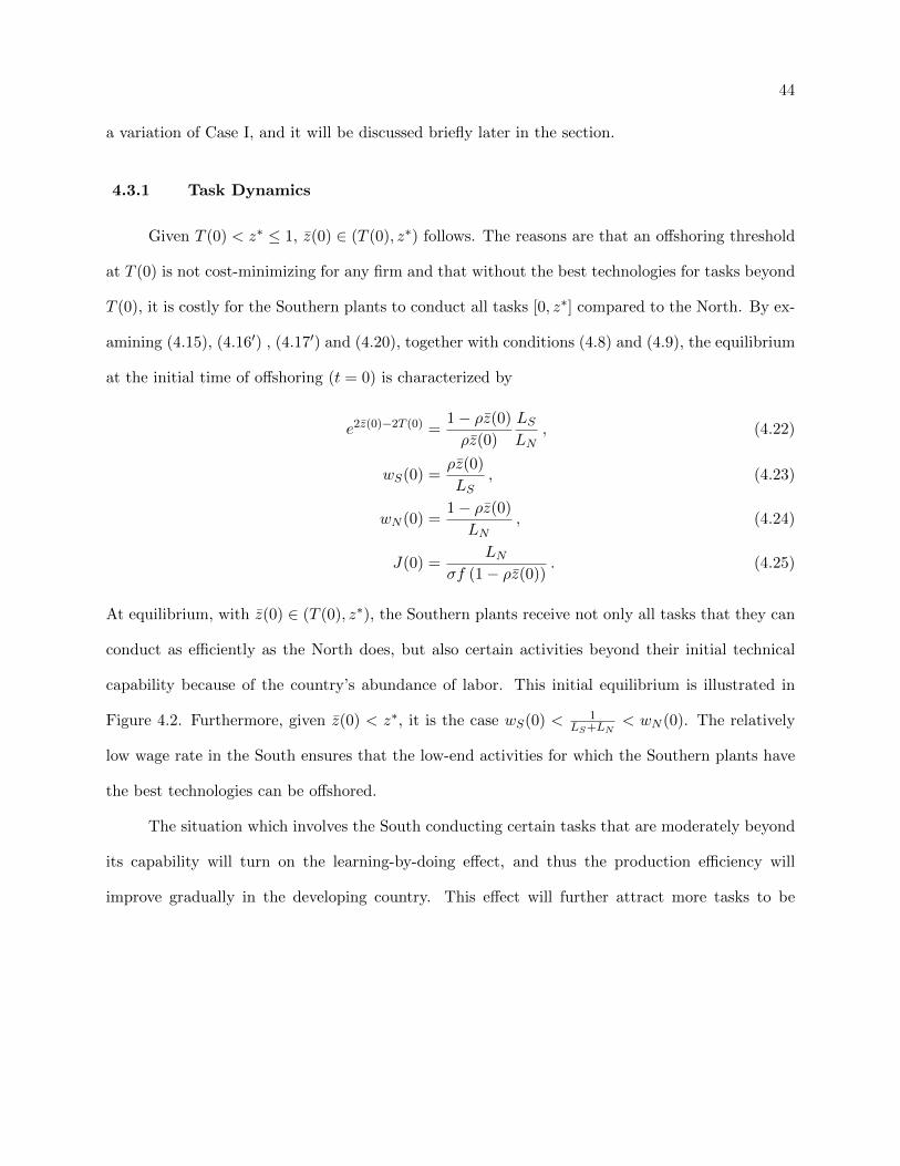
44

a variation of Case I, and it will be discussed briefly later in the section.

4.3.1 Task Dynamics

Given T (0) < z∗ ≤ 1, z(0) ∈ (T (0), z∗) follows. The reasons are that an offshoring threshold

at T (0) is not cost-minimizing for any firm and that without the best technologies for tasks beyond

T (0), it is costly for the Southern plants to conduct all tasks [0, z∗] compared to the North. By ex-

amining (4.15), (4.16′) , (4.17′) and (4.20), together with conditions (4.8) and (4.9), the equilibrium

at the initial time of offshoring (t = 0) is characterized by

e2z(0)−2T (0) =1− ρz(0)

ρz(0)

LSLN

, (4.22)

wS(0) =ρz(0)

LS, (4.23)

wN (0) =1− ρz(0)

LN, (4.24)

J(0) =LN

σf (1− ρz(0)). (4.25)

At equilibrium, with z(0) ∈ (T (0), z∗), the Southern plants receive not only all tasks that they can

conduct as efficiently as the North does, but also certain activities beyond their initial technical

capability because of the country’s abundance of labor. This initial equilibrium is illustrated in

Figure 4.2. Furthermore, given z(0) < z∗, it is the case wS(0) < 1LS+LN

< wN (0). The relatively

low wage rate in the South ensures that the low-end activities for which the Southern plants have

the best technologies can be offshored.

The situation which involves the South conducting certain tasks that are moderately beyond

its capability will turn on the learning-by-doing effect, and thus the production efficiency will

improve gradually in the developing country. This effect will further attract more tasks to be

45

Figure 4.2: Initial Task Offshoring: Normal Evolution (T (0) < z∗ ≤ 1)

0 1


z

North

South at t=0

T(0) z(0) z*

offshored. At time t, the instantaneous equilibrium is characterized by

e2z(t)−2T (t) =1− ρz(t)ρz(t)

LSLN

, (4.22′)

wS(t) =ρz(t)

LS, (4.23′)

wN (t) =1− ρz(t)LN

, (4.24′)

J(t) =LN

σf (1− ρz(t)). (4.25′)

Following the same logic as discussed for the initial equilibrium, as long as T (t) < z∗, it is always

the case that the offshoring threshold lies between the South’s technology stock and the offshoring

steady state (i.e., z(t) ∈ (T (t), z∗)), which enables the South to learn. During the process, the wage

rate in the South is always lower than the Northern wage level (i.e., wS(t) < 1LS+LN

< wN (t)).

The positive learning effect in the South is reflected by the accumulation of technology in

the country. The technology-stock indicator T (t) evolves over time according to the technology

accumulation path:8

dT (t)

dt=βLSJ(t)

z(t)− T (t)

z(t)= βσf (1− ρz(t)) LS

LN

z(t)− T (t)

z(t). (4.26)

8 See Appendix B.1.1 for the derivation of (4.26).

46

The learning effect implies that as long as the Southern plants perform certain tasks beyond their

technical capability (z(t) > T (t)), they can always learn from what they conduct (i.e., dT (t)dt > 0).

This positive learning-by-doing effect pushes the offshoring threshold further, with the South-

ern coverage of task‘ expanding to include more sophisticated activities. Namely, if the set of tasks

undertaken in a plant is viewed as the scope of the plant, then the learning effect will lead to scope

expansion in the Southern plants. This can be seen by examining (4.22′):

dz(t)

dt=

2z(t) (1− ρz(t))1 + 2z(t) (1− ρz(t))

× dT (t)

dt, (4.27)

which implies

0 <dz(t)

dt<dT (t)

dt, (4.28)

as long as the learning room is not exhausted. With learning, the Southern plants are capable of

conducting tasks increasingly efficiently for those tasks at which they were not competent before;

together with a relatively low wage rate, the South attracts more and harder tasks to be undertaken

there. Certainly, while a wider range of low-sophistication tasks are being offshored to the South,

the North increasingly focuses on the most difficult activities ((z(t), 1]). Therefore, both low-

income and high-income countries move up the global value chain over time – they both experience

upgrading in the sets of tasks that their firms conduct.

As indicated by (4.26), how strong the learning effect is depends upon the relative learning

opportunities for the South – for which tasks there is still room for technology improvement, relative

to all tasks that are actually offshored (i.e., the distance between T (t) and z(t)). As time passes,

with dT (t)dt > dz(t)

dt , the initial learning opportunities are gradually exhausted, which will in turn

slow down the pace of learning over time.9 This further translates into a concave-shaped time

path of offshoring evolution. As global production evolves, it is the case that10

d2T (t)

dt2< 0, and

d2z(t)

dt2< 0 . (4.29)

9 This pattern is not hard to tell from (4.26). The increase in z(t) with decrease in (z(t) − T (t)) leads dT (t)dt

todecline over time.

10 See Appendix B.1.1 and Appendix B.1.2 for proof.

47

In the long run, both the technology stock in the South and the offshoring threshold converge

to the same steady state, z∗.11 When they arrive at the steady state, they will not grow further

beyond it. With equalized wage rates and both countries possessing the same best technologies for

tasks conducted domestically, the pattern of global production is stabilized.

In sum, the dynamics of both the technology stock in the South (T (t)) and the task-threshold

of offshoring (z(t)) display concave-shaped growth paths, both converging to the same steady state,

which serves as the upper bound. The convergence process is demonstrated in Figure 4.3.

Figure 4.3: Dynamics of Task Offshoring: Normal Evolution (T (0) < z∗ ≤ 1)

0

z(t)

T(t)

t

z*

Certainly, factors such as the learning ability of the South (indicated by β), fixed cost (f),

variety substitutability of the industry (σ, and thus ρ), and the countries’ labor endowments (LS

and LN ) all have influence on the convergence paths. Numerical simulations are performed here

to examine how different variables may affect the evolution dynamics of global production. Figure

4.4 demonstrates the results of the numerical simulations. Panel A shows that the size of a country

can compensate for its production inefficiency – a larger although technically inefficient country

gets a wider range of tasks to carry out, both in the short run and in the long run. Panel B

shows the results from variation in the learning ability of the South. It is obvious that a Southern

11 This can be seen by examining (4.22′) at z∗.

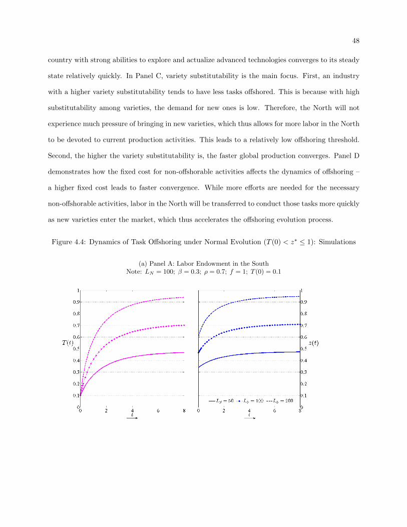
48

country with strong abilities to explore and actualize advanced technologies converges to its steady

state relatively quickly. In Panel C, variety substitutability is the main focus. First, an industry

with a higher variety substitutability tends to have less tasks offshored. This is because with high

substitutability among varieties, the demand for new ones is low. Therefore, the North will not

experience much pressure of bringing in new varieties, which thus allows for more labor in the North

to be devoted to current production activities. This leads to a relatively low offshoring threshold.

Second, the higher the variety substitutability is, the faster global production converges. Panel D

demonstrates how the fixed cost for non-offshorable activities affects the dynamics of offshoring –

a higher fixed cost leads to faster convergence. While more efforts are needed for the necessary

non-offshorable activities, labor in the North will be transferred to conduct those tasks more quickly

as new varieties enter the market, which thus accelerates the offshoring evolution process.

Figure 4.4: Dynamics of Task Offshoring under Normal Evolution (T (0) < z∗ ≤ 1): Simulations

(a) Panel A: Labor Endowment in the SouthNote: LN = 100; β = 0.3; ρ = 0.7; f = 1; T (0) = 0.1

49

(b) Panel B: Learning AbilityNote: LS = 100; LN = 100; ρ = 0.7; f = 1; T (0) = 0.1

(c) Panel C: Variety SubstitutabilityNote: LS = 100; LN = 100; β = 0.3; f = 1; T (0) = 0.1

4.3.2 Variety Dynamics

Under monopolistic competition, consumers’ love for variety provides the market with the

incentive to create and maintain different brands. With more and more tasks relocated to the

South, the labor in the North that was previously devoted to those offshorable tasks can now

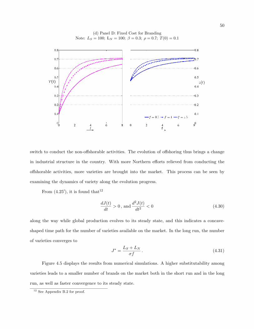
50

(d) Panel D: Fixed Cost for BrandingNote: LS = 100; LN = 100; β = 0.3; ρ = 0.7; T (0) = 0.1

switch to conduct the non-offshorable activities. The evolution of offshoring thus brings a change

in industrial structure in the country. With more Northern efforts relieved from conducting the

offshorable activities, more varieties are brought into the market. This process can be seen by

examining the dynamics of variety along the evolution progress.

From (4.25′), it is found that12

dJ(t)

dt> 0 , and

d2J(t)

dt2< 0 (4.30)

along the way while global production evolves to its steady state, and this indicates a concave-

shaped time path for the number of varieties available on the market. In the long run, the number

of varieties converges to

J∗ =LS + LN

σf. (4.31)

Figure 4.5 displays the results from numerical simulations. A higher substitutability among

varieties leads to a smaller number of brands on the market both in the short run and in the long

run, as well as faster convergence to its steady state.

12 See Appendix B.2 for proof.

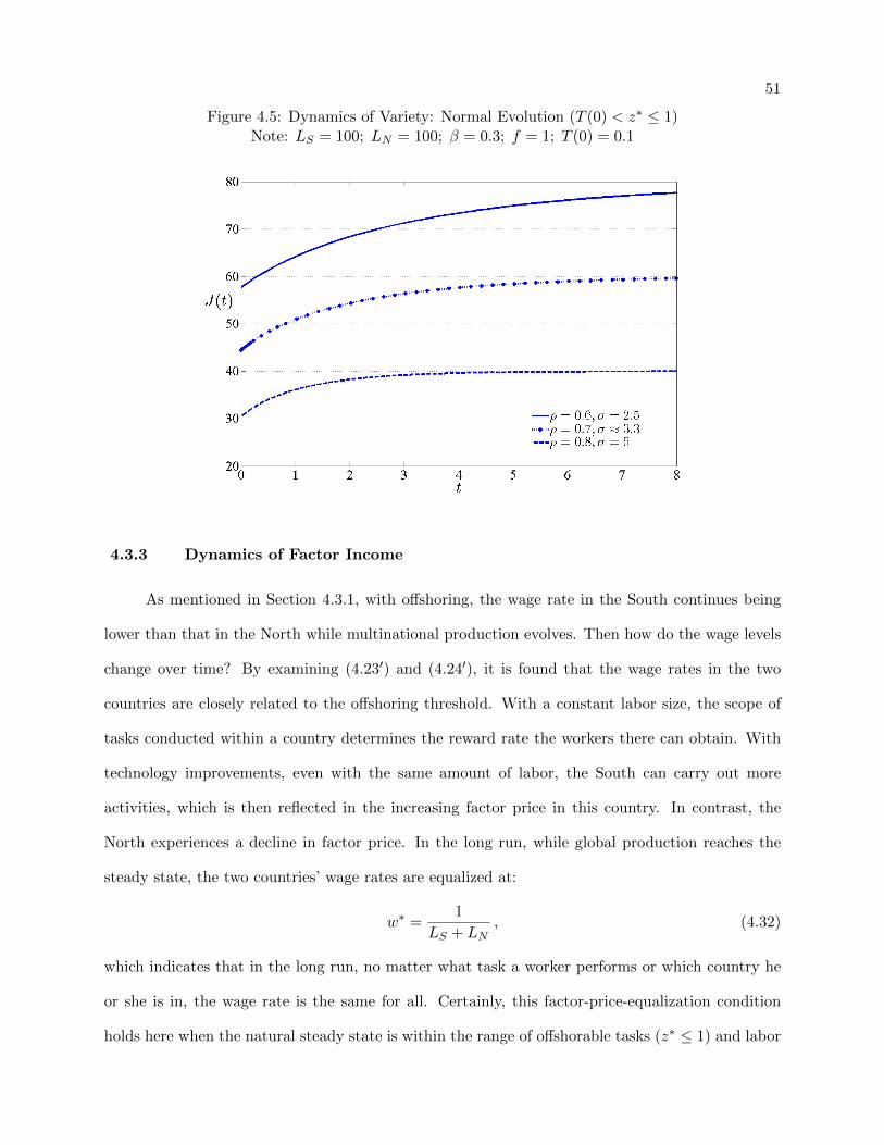
51

Figure 4.5: Dynamics of Variety: Normal Evolution (T (0) < z∗ ≤ 1)Note: LS = 100; LN = 100; β = 0.3; f = 1; T (0) = 0.1

4.3.3 Dynamics of Factor Income

As mentioned in Section 4.3.1, with offshoring, the wage rate in the South continues being

lower than that in the North while multinational production evolves. Then how do the wage levels

change over time? By examining (4.23′) and (4.24′), it is found that the wage rates in the two

countries are closely related to the offshoring threshold. With a constant labor size, the scope of

tasks conducted within a country determines the reward rate the workers there can obtain. With

technology improvements, even with the same amount of labor, the South can carry out more

activities, which is then reflected in the increasing factor price in this country. In contrast, the

North experiences a decline in factor price. In the long run, while global production reaches the

steady state, the two countries’ wage rates are equalized at:

w∗ =1

LS + LN, (4.32)

which indicates that in the long run, no matter what task a worker performs or which country he

or she is in, the wage rate is the same for all. Certainly, this factor-price-equalization condition

holds here when the natural steady state is within the range of offshorable tasks (z∗ ≤ 1) and labor

52

flows freely among offshorable and non-offshorable tasks in the North. In the other cases where

the potential steady state z∗ goes beyond the range of offshorable tasks (z∗ > 1) so that the actual

steady state is at z∗′ = 1, the situation is different and will be discussed in later sections.

The wage rate dynamics in the South shows a concave-shaped path, while in the North it

displays a convex one, both converging to the steady-state wage rate w∗.13 Figure 4.6 demonstrates

the wage dynamics of the two countries.14

Figure 4.6: Dynamics of Wage Rates: Normal Evolution (T (0) < z∗ ≤ 1)

0 t

w*

wN(t)

wS(t)

It is clear that although the wage gap between the two countries exists initially in the short

run, it diminishes over time as tasks are increasingly offshored. In the long run, under normal

offshoring, the wage gap may be closed with factor prices equalized. At the steady state, workers

in the South enjoy the same income level as their Northern counterparts, even though they do

not master all the most advanced technologies. Hence, what matters most for workers is the

actualization of technologies, rather than the potential productivities that are not embodied in real

production.

13 From (4.23′) and (4.24′), dwS(t)dt

= ρLS

dz(t)dt≥ 0, d2wS(t)

dt2= ρ

LS

d2z(t)

dt2≤ 0; dwN (t)

dt= − ρ

LN

dz(t)dt≤ 0, d2wN (t)

dt2=

− ρLN

d2z(t)

dt2≥ 0.

14 Wage rates here are expressed as a share of the world expenditure, since E(t) has been normalized to 1.

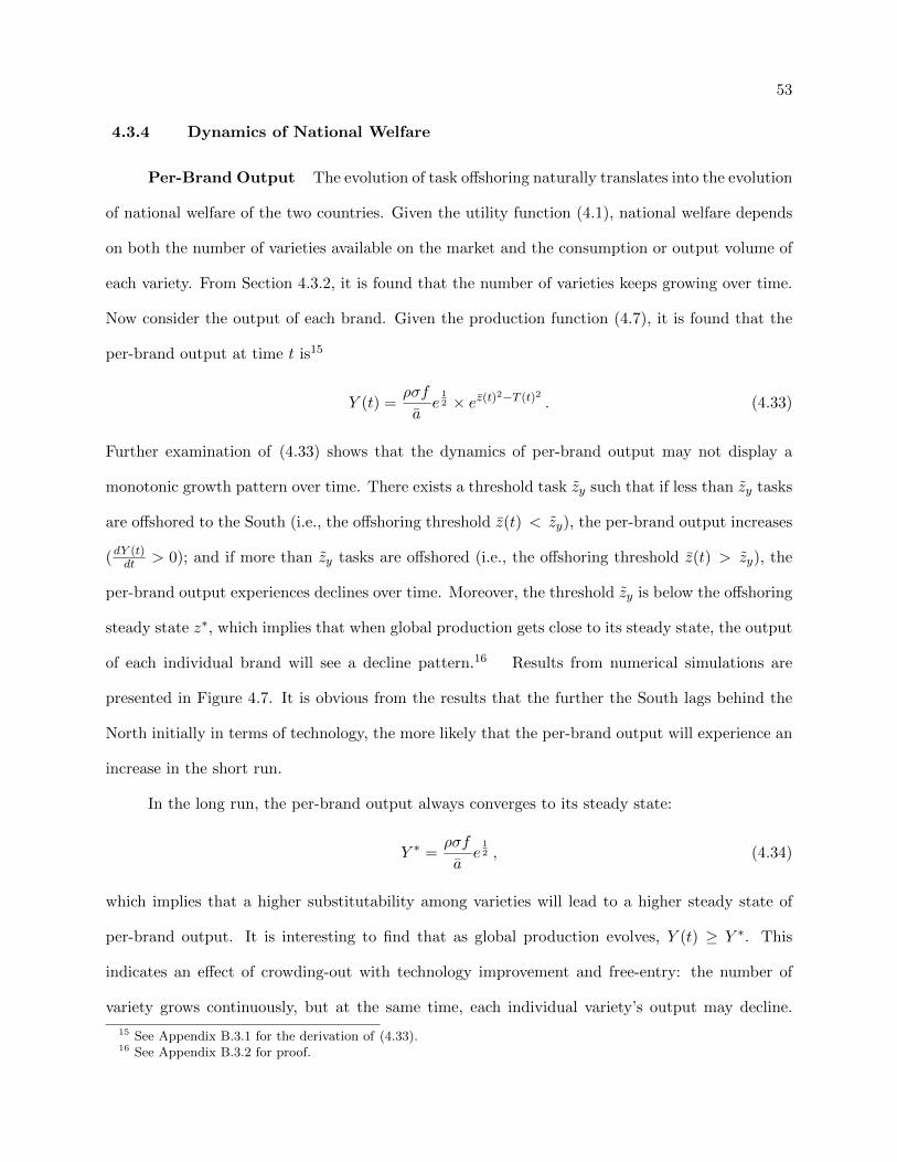
53

4.3.4 Dynamics of National Welfare

Per-Brand Output The evolution of task offshoring naturally translates into the evolution

of national welfare of the two countries. Given the utility function (4.1), national welfare depends

on both the number of varieties available on the market and the consumption or output volume of

each variety. From Section 4.3.2, it is found that the number of varieties keeps growing over time.

Now consider the output of each brand. Given the production function (4.7), it is found that the

per-brand output at time t is15

Y (t) =ρσf

ae

12 × ez(t)2−T (t)2

. (4.33)

Further examination of (4.33) shows that the dynamics of per-brand output may not display a

monotonic growth pattern over time. There exists a threshold task zy such that if less than zy tasks

are offshored to the South (i.e., the offshoring threshold z(t) < zy), the per-brand output increases

(dY (t)dt > 0); and if more than zy tasks are offshored (i.e., the offshoring threshold z(t) > zy), the

per-brand output experiences declines over time. Moreover, the threshold zy is below the offshoring

steady state z∗, which implies that when global production gets close to its steady state, the output

of each individual brand will see a decline pattern.16 Results from numerical simulations are

presented in Figure 4.7. It is obvious from the results that the further the South lags behind the

North initially in terms of technology, the more likely that the per-brand output will experience an

increase in the short run.

In the long run, the per-brand output always converges to its steady state:

Y ∗ =ρσf

ae

12 , (4.34)

which implies that a higher substitutability among varieties will lead to a higher steady state of

per-brand output. It is interesting to find that as global production evolves, Y (t) ≥ Y ∗. This

indicates an effect of crowding-out with technology improvement and free-entry: the number of

variety grows continuously, but at the same time, each individual variety’s output may decline.

15 See Appendix B.3.1 for the derivation of (4.33).16 See Appendix B.3.2 for proof.

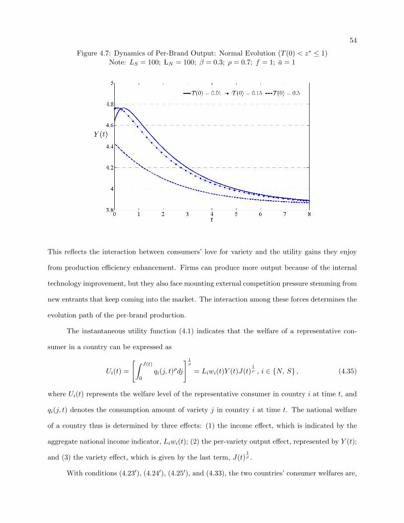
54

Figure 4.7: Dynamics of Per-Brand Output: Normal Evolution (T (0) < z∗ ≤ 1)Note: LS = 100; LN = 100; β = 0.3; ρ = 0.7; f = 1; a = 1

This reflects the interaction between consumers’ love for variety and the utility gains they enjoy

from production efficiency enhancement. Firms can produce more output because of the internal

technology improvement, but they also face mounting external competition pressure stemming from

new entrants that keep coming into the market. The interaction among these forces determines the

evolution path of the per-brand production.

The instantaneous utility function (4.1) indicates that the welfare of a representative con-

sumer in a country can be expressed as

Ui(t) =

[∫ J(t)

0qi(j, t)

ρdj

] 1ρ

= Liwi(t)Y (t)J(t)1ρ , i ∈ N, S , (4.35)

where Ui(t) represents the welfare level of the representative consumer in country i at time t, and

qi(j, t) denotes the consumption amount of variety j in country i at time t. The national welfare

of a country thus is determined by three effects: (1) the income effect, which is indicated by the

aggregate national income indicator, Liwi(t); (2) the per-variety output effect, represented by Y (t);

and (3) the variety effect, which is given by the last term, J(t)1ρ .

With conditions (4.23′), (4.24′), (4.25′), and (4.33), the two countries’ consumer welfares are,

55

respectively,

US(t) = ρ×(LNσf

) 1ρ

× ρσf

a× e

12 ×

[z(t) (1− ρz(t))−

1ρ ez(t)

2−T (t)2], (4.36)

and

UN (t) =

(LNσf

) 1ρ

× ρσf

a× e

12 ×

[(1− ρz(t))1− 1

ρ ez(t)2−T (t)2

]. (4.37)

Dynamics of welfare in the South Examining the South’s consumer welfare indicated

by (4.36), it is found that the utility level enjoyed by Southern consumers keeps increasing since the

initial time t = 0 (i.e., dUS(t)dt > 0), until global production reaches the steady state.17 Therefore,

for the South, although the world output of each brand may experience a decline over time, the

other two effects, i.e., the income effect and the variety effect, are positive and dominate the

evolution.18 With increasing income and a growing number of varieties, the South keeps enjoying

welfare improvements while taking more and more production tasks. In the long run, the national

welfare of the South reaches its steady state:

U∗S =LS

LS + LN×(LS + LN

σf

) 1ρ

× ρσf

a× e

12 . (4.38)

Dynamics of welfare in the North For the North, the situation is different. Among

the three effects, the national income decreases for the North, which can be seen from (4.24′). The

per-variety output also decreases when global production gets close to the steady state. The only

effect that keeps experiencing positive growth is the number of varieties. By examining (4.37), it is

found that the national welfare of the North may be non-monotonic over time. There is a threshold

zUN that serves as a stationary point. If the offshoring threshold (z(t)) is right at zUN , it is the case

that dUN (t)dt = 0. When less than zUN tasks are allocated to the Southern plants for completion

(z(t) < zUN ), the consumers in the North experience growth in their utility (dUN (t)dt > 0). In

contrast, when more than zUN tasks are offshored (z(t) > zUN ), the Northern welfare declines over

time (dUN (t)dt < 0). This stationary point is further found to be higher than zy.

19

17 See Appendix B.4.1 for proof.18 This could be seen from conditions (4.23′), (4.28) and (4.30).19 See Appendix B.4.2 for proof.

56

Therefore, after the per-brand output reaches the peak amount and when it starts to decline,

the consumers in the North can still enjoy an increasing utility for an extended period of time,

during which the variety effect dominates the other two, while both the national income and the

production of each variety decrease. Consequently, Northern consumers’ utility has two possible

different evolution paths. In the first case, the South initially receives relatively few tasks, with

z(0) < zUN . The variety effect, possibly with a positive output effect, is significant so that the

Northern consumers get increasingly better off in the short run. This trend is reversed after more

than zUN tasks are offshored. The other possible path happens when the Southern plants obtain

a relatively large range of activities initially beyond zUN , which will lead the North to experience

persistent declines in welfare until the steady state is reached. No matter which path is realized,

the steady-state level of Northern welfare is

U∗N =LN

LS + LN×(LS + LN

σf

) 1ρ

× ρσf

a× e

12 (4.39)

in the long run. Compared with the initial level UN (0), the long-run steady-state welfare U∗N is not

necessarily higher or lower. The interaction among the three effects, as well as the initial situation,

determines where the final case is.

Figure 4.8 displays results from simulations with different parameter values. Panel A displays

how the variety substitutability may affect the two countries’ welfare dynamics. For both countries,

the lower the substitutability is, the higher the long-run welfares are at the steady state. This

implies that consumers’ love for variety is important in the sense that it can strengthen and enlarge

the variety effect on national welfare, which is always positive for both countries among the three.

Panel B shows the situations with different relative Southern labor endowments. The results show

that a larger South engaging in offshoring can bring both countries higher welfares. Thus, for

technologically advanced countries, it is to their benefit to cooperate with developing countries

with relatively large factor supplies. Compared with small ones, a large developing host country

has more resources that can be devoted to learning in global production,20 which empowers a

20 Consider that the offshoring threshold at the steady state is relatively high.

57

bigger improvement in technologies. This will lead to more products and varieties being produced

and thus to a higher national welfare.

Figure 4.8: Dynamics of National Welfare under Normal Evolution (T (0) < z∗ ≤ 1): Simulations

(a) Panel A: Variety SubstitutabilityNote: LS = 100; LN = 100; β = 0.3; f = 1; T (0) = 0.01; a = 1

(b) Panel B: Size of the SouthNote: LN = 100; β = 0.3; ρ = 0.7; f = 1; T (0) = 0.1; a = 1

58

4.3.5 Extreme-End Evolution

In the case of extreme-end evolution, the potential steady state z∗ is beyond the range of

offshorable tasks (z∗ > 1), which thus leads the actual steady state of global production to be

z∗′ = 1 in the long run. The most sophisticated offshorable task serves as the upper bound of

offshoring, where global production saturates. Therefore, all offshorable tasks will be offshored to

the South in the long run under this circumstance – theoretically, a situation that may happen if

the South is sufficiently abundant in production factors relative to the North. The North will then

focus solely on the non-offshorable activities.

Task Offshoring Dynamics The dynamics of variables are essentially variations of the

normal-evolution situation. With both the South’s initial technology stock T (0) and the initial

offshoring threshold z(0) within the task range (0, 1), all aspects of the two economies behave as

if the steady state is z∗ at the beginning. Thus, the dynamics of task offshoring at first displays

a pattern of convergence similar to the corresponding one discussed in the normal-evolution case.

Once all offshorable tasks have been allocated to the South (z(tz) = 1), further offshoring will not

happen. However, the South’s technical capability will continue improving for some time, until

it matches the range of tasks offshored (T (t∗′) = 1,with t∗′ > tz). The evolution paths of task

offshoring and technology stock are shown in Figure 4.9. The left panel displays the potential

dynamics if the offshorable tasks’ range could go beyond z = 1. The right panel shows the actual

dynamics of the technology stock T (t) and the offshoring threshold z(t) over time. Offshoring

stops progressing when the offshoring threshold reaches the upper bound. After that, the South’s

technological capability continues improving, although the speed of learning is lower compared with

the potential case.21 The actual steady state will be arrived at when the technology stock in the

South matches the offshoring pattern (T ∗′ = z∗′ = 1).

Factor Price and Number of Varieties Consider other variables characterizing the

economies, such as the wage rates and the number of varieties. At first, before the South obtains

all offshorable activities to conduct (z(t) < 1), they all follow the same corresponding paths of

21 This can be understood by examining equation (4.26).

59

Figure 4.9: Task Dynamics under Extreme-End Evolution (z∗ > 1, z∗′ = 1)Note: LN = 100 ;LS = 100 ;β = 0.3 ; ρ = 0.4 ; f = 1 ;T (0) = 0.1

evolution as what they would experience if the task range could go beyond z = 1. Then when all

offshorable tasks are moved to the South, the wage rates in the two countries stop changing. Thus,

their evolution paths are not smooth – the time when offshoring hits its upper limit is a singular

point when the wage rates reach their bounds and also their final steady states. Given that z∗′ = 1,

the factor prices in the long run are w∗′S = ρLS

and w∗′N = 1−ρLN

respectively, with w∗′S < w∗′N .22

Therefore, the factor-price-equalization condition is not achieved in this case. For the number

of varieties, the situation is similar. It stops growing once all offshorable tasks are allocated to

the Southern plants. With all Northern efforts solely spent on non-offshorable activities, the total

number of varieties on the market is given by J∗′ = LNf in the long run. Figure 4.10 presents the

evolution paths for wage rates and for the number of varieties.

Output and Welfares Production efficiency is the key factor determining output and

thus national welfare levels. After the offshoring threshold stops moving further, the learning effect

continues being positive in the South for some time, but is weaker than it would be if there was no

22 Consider that z∗ = LSρ(LS+LN )

> 1 in this case.

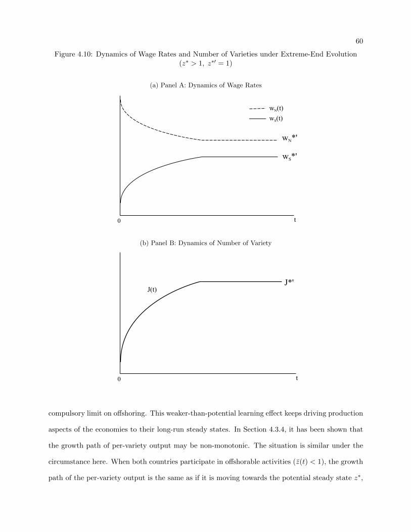
60

Figure 4.10: Dynamics of Wage Rates and Number of Varieties under Extreme-End Evolution(z∗ > 1, z∗′ = 1)

(a) Panel A: Dynamics of Wage Rates

0 t

wN*'

wN(t)

wS(t)

wS*'

(b) Panel B: Dynamics of Number of Variety

0 t

J*'J(t)

compulsory limit on offshoring. This weaker-than-potential learning effect keeps driving production

aspects of the economies to their long-run steady states. In Section 4.3.4, it has been shown that

the growth path of per-variety output may be non-monotonic. The situation is similar under the

circumstance here. When both countries participate in offshorable activities (z(t) < 1), the growth

path of the per-variety output is the same as if it is moving towards the potential steady state z∗,

61

and it may or may not show positive growth in the short-run. When all offshorable tasks have been

allocated to the South (z(t) = 1), the per-brand output starts to be described by23

Y (t)′ =LSf

LN a× e−(T (t)−1)2+ 1

2 , (4.40)

which increases over time while the South improves its technology.24 In the long run, it converges

to its steady state

Y ∗′ =LSf

LN ae

12 , (4.41)

when the South has possessed the most advanced technologies for all tasks. Compared with the

normal-evolution case, if the South takes all offshorable production responsibilities, in the long run,

there will be more brands on the market(J∗′ > J∗), while less of each is supplied (Y ∗′ < Y ∗).

With regard to national welfare, before the offshoring threshold z(t) reaches the most sophis-

ticated offshorable task, like in the normal-evolution case, the South experiences positive growth

since the very beginning of engaging in global production, while the North may see different pos-

sible patterns of growth over time. However, during the period of time when all tasks have been

offshored and the South is still learning (z(t) = 1 and T (t) < 1), both countries will experience

welfare growth. Specifically, with the per-brand output expression derived above, during this time

period, the national welfares of the two countries are, respectively,

US(t)′ = ρ×(LNf

) 1ρ−1

× LSa× e−(T (t)−1)2+ 1

2 , (4.42)

and

UN (t)′ = (1− ρ)×(LNf

) 1ρ−1

× LSa× e−(T (t)−1)2+ 1

2 . (4.43)

Both of them will be increasing monotonically while T (t) < 1 and dT (t)dt > 0. When the South’s

technology stock covers the most sophisticated task, the welfares converge to their steady states:

U?′S = ρ

(LNf

) 1ρ−1 LS

ae

12 , (4.44)

23 See Appendix B.5.1 for derivation of (4.40).24 See Appendix B.5.2 for proof.

62

and

U?′N = (1− ρ)

(LNf

) 1ρ−1 LS

ae

12 . (4.45)

With the discussion above and in Section 4.3.4, it is found that during the process of evolving, the

South continues seeing welfare improvement, although the speed of improvement may decrease. For

the North, the overall path of welfare development may be non-monotonic. Numerical simulations

are performed for per-brand output as well as for national welfares. The results are shown in Figure

4.11. Panel A displays the simulation results for the per-brand output. After all manufacturing

tasks are offshored to the South, the learning effect stimulates another round of output growth.

For the national welfare results displayed in Panel B, the South sees positive increases in national

utility during the whole evolution process. For the North, although the initial growth pattern is

uncertain, after all manufacturing tasks are taken by the South, the country will also experience

positive growth – the learning effect will benefit both countries by increasing the output of each

brand.

Figure 4.11: Dynamics of Output and Welfares under Extreme-End Evolution (z∗ > 1, z∗′ = 1)

(a) Panel A: Dynamics of Per-Brand OutputNote: LS = 100; LN = 100; β = 0.3; ρ = 0.4; f = 1; a = 1

63

(b) Panel B: Dynamics of National WelfaresNote: LS = 10; LN = 10; β = 0.3; f = 1; T (0) = 0.3; a = 1

4.3.6 Static Equilibrium Cases

Except for the dynamic situations where countries see evolutions of their multinational op-

erations, there are two other static equilibrium possibilities: Case III – static normal offshoring, in

which the South’s initial technology stock is sufficiently high so that global production reaches its

normal steady state z∗ ∈ (0, 1) at the initial time t = 0; and Case IV – static complete offshoring,

where since the very beginning, the South is essentially the same as the North in terms of technol-

ogy (T (0) = 1), and the factor endowment of the South is abundant so that all offshorable tasks

are moved to the South since t = 0.

The static normal offshoring situation is likely to happen if the South is technically capable

and relatively small in size, so that T (0) ≥ z∗. When this situation prevails, there will be no room

for the South to learn, as the country is not working on any activity at which it is not already

skilled. Therefore, the world equilibrium stays at z∗ since t = 0, with all other aspects of the two

economies at their steady states since the initial time.

The other static case is essentially a multinational production situation with two countries

equally advanced in terms of technology on conducting the offshorable activities. The South is

64

relatively large such that z∗ > 1 and z(0) = 1. If this is the case, then the country with abundant

factor endowment will be specializing in offshorable tasks, while the other one puts all efforts on

the non-offshorable activities. Learning is not present here as both countries already possess the

best technologies since the beginning. Therefore, this pattern of specialization will hold as long as

factor supplies remain stable. The two economies are at the steady states characterized by z∗′ = 1.

4.4 Gains from Offshoring

The discussion so far focuses on the time dynamics of offshoring evolution. It has been shown

that compared with the initial situation when the two countries start engaging in offshoring, the

South becomes increasingly better off over time, while the North may or may not see a higher

welfare level at the long-run steady state. Then the question becomes whether the countries should

participate in global production by offshoring or accepting offshored activities, or they should

remain closed and supply all products domestically.

4.4.1 Equilibrium under Autarky

The consumer preferences are still identical in the two countries under autarky, described by

the same C.E.S. function (4.1). The production of goods, as well as the two countries’ produc-

tion technologies, is also the same as defined in Section 4.1.3. Namely, the two economies start

with the situations under autarky the same as under offshoring. Under autarky, countries do not

have information about each other, and thus they are not able to acknowledge their technological

differences in production. Without seeing the gap, the South does not have incentives to learn,

though it conducts all the activities under this circumstance. Therefore, under autarky, there is

no production efficiency improvement over time like what we have seen under offshoring. Since

countries’ behaviors do not change over time, the time index t can be omitted here.

In autarky, both countries have to conduct all activities on the task range [0, 1] to produce

the final goods, and both of them also need to pay the fixed costs, which are assumed to be the

same (f), to make the products viewable on the market. Let EAi denote the national expenditure

65

on final products in country i under autarky, defined as the sum of factor payments in that country:

EAi = wAi Li , i ∈ N, S , (4.46)

where wAi denotes the autarky wage rate of country i.

Assume that the fixed cost is the same across countries: fS = fN = f . The labor market

clearing conditions for the two economies under autarky are given by

South :

∫ 1

0xAS (z)a(z, 0)dz + JAS f = LS ,

North :

∫ 1

0xAN (z)a(z)dz + JANf = LN ,

where xAi (z) denotes the total amount of task z conducted in country i by all firms there, and JAi

denotes the number of brands on the market in country i, both under autarky. The task demands

can be expressed as:

xAS (z) =ρEAS

wAS a(z, 0)=

ρLSa(z, 0)

,

xAN (z) =ρEANwAN a(z)

=ρLNa(z)

.

With the task demands, the labor market clearing conditions become:

South :

∫ 1

0ρLSdz + JAS f = LS , (4.47)

North :

∫ 1

0ρLNdz + JANf = LN . (4.48)

The numbers of varieties in the two domestic markets thus are:

JAi =Liσf

, i ∈ N, S . (4.49)

Given the production function (4.7), together with the task demand expressions, technology

specifications (4.8) and (4.9), and condition (4.49), the per-brand outputs under autarky are found

to be

Y AS =

ρσf

a× e−(T (0)−1)2+ 1

2 , (4.50)

66

and

Y AN =

ρσf

a× e

12 . (4.51)

Together with the number of varieties JAi , this implies that the national utility levels of the two

countries are, respectively,

UAS =

(LSσf

) 1ρ

× ρσf

a× e−(T (0)−1)2+ 1

2 , (4.52)

and

UAN =

(LNσf

) 1ρ

× ρσf

a× e

12 , (4.53)

which remain constant over time.

4.4.2 Gains from Normal Offshoring

Under normal offshoring, global production is characterized by the participation of both

countries in offshorable tasks, in the short run as well as in the long run. During the process of

normal evolution, the national welfares are given by (4.36) and (4.37).

Gains of the South For the South, comparing the welfare under offshoring and the welfare

under autarky, it is found that

US(t)

UAS=

[LNLS× 1

1− ρz(t)

] 1ρ

×[ρz(t)× ez(t)2−T (t)2 × e(T (0)−1)2

]. (4.54)

Countries’ welfare levels essentially depend on the number of varieties available on the market and

the consumption or output of each product. The first term of the equation above indicates the

variety effect (the extensive margin), while the second implies the output (or consumption) effect

(the intensive margin).

When the South opens to offshoring, the Southern labor that was working on non-offshorable

tasks is withdrawn and reassigned to conduct the offshored activities. Therefore, the number of

goods available is no longer totally determined within the country, while the North takes over

certain responsibilities. This international shift of non-offshorable efforts brings uncertainty with

regard to whether the developing country can enjoy more variety options initially when countries

67

start to engage in global production. During the initial stages when offshoring starts, the South may

or may not be able to obtain the same number of varieties as they could under autarky. Then as

time elapses, the situation improves. While more and more tasks are reallocated to the South which

enables more Northern efforts to be put on non-offshorable activities, both countries’ consumers

can enjoy more variety options over time. In the long run, it is found that J∗

JAS= LS+LN

LS> 1, which

indicates that with offshoring and learning, the Southern consumers will enjoy more varieties than

they could under autarky. By participating in global production, the South not only obtains better

technologies, but also enjoys more options for consumption. This variety effect contributes to the

long-run welfare gain of the country.

Concerning the output effect, it is not definite that the South can enjoy more consumption

on each brand at the initial time when it starts producing for the whole world. The output also

depends on the North’s conditions. In the long run, the output effect indicated by the second term

of (4.54) turns out to be indefinite as well.25

Combining the two effects, both the variety and the output effects, it is found that

U∗SUAS

=

[LS + LN

LS

] 1ρ−1

× e(T (0)−1)2

> 1 . (4.55)

Therefore, although the gain from engaging in global production is not definite for the South in the

short run, it will certainly benefit the South in the long run. This is different from the offshoring

case under perfect competition discussed in Chapter 3, where the South sees gains in both the

short run and the long run. By accepting offshored activities and by learning in the process of

conducting them, the South under monopolistic competition may experience short-run pains, but

it will end up enjoying more consumption choices, which dominates the other welfare effect.

Gains of the North Consider the situation for the North. By comparing (4.37) and

(4.53), it is the case that

UN (t)

UAN=

[1

1− ρz(t)

] 1ρ

×[(1− ρz(t))× ez(t)2−T (t)2

]> 1 , (4.56)

25 When the global economy reaches the steady state z∗, the second term becomes: ρz∗ × e(T (0)−1)2 = LSLS+LN

×e(T (0)−1)2 , which is not necessarily greater or less than 1.

68

which is greater than 1 since the initial time of offshoring (t = 0). The first term in the equation

is the variety effect for the North, while the second indicates the consumption or output effect.

By relocating low-sophistication tasks to the South, the North is able to produce more va-

rieties since the very beginning of offshoring. Thus, the variety effect is positive initially and will

continue strengthening over time as more and more production tasks are offshored. The other one,

the per-brand consumption effect, is not deterministic for the North, but it is dominated by the

variety effect, which then leads to the situation where the North overall is better off than under

autarky since the start of engaging in global production. In the long run, the utility comparison

shows that the North ultimately benefits from offshoring:

U∗NUAN

=

[LS + LNLN

] 1ρ−1

> 1. (4.57)

In sum, from the analyses above, participating in global production is beneficial for both

countries. Even if they may experience short-term challenges when they initially join in the global

production network and/or during the process in which they are evolving to the steady state, they

both will ultimately see positive gains and rewards from offshoring. The results from simulations

clearly demonstrate this pattern, and are shown in Figure 4.12. In the simulation, although both

countries initially experience a cut in per-brand consumption when they join in global production,

they do see welfare gains in the long run compared with autarky. This also further confirms that

for the static normal offshoring case, although learning is not present, both countries can still earn

positive gains by forming a multinational production network.

4.4.3 Gains from Extreme-End Offshoring

In the case of extreme-end offshoring, in the long run, all offshorable tasks are ultimately

allocated to the South. During the process of evolution, as discussed in the previous section, the

South may experience short-run challenges while the North is always better off compared with the

autarky situation. Consider the long-run welfare at the steady state. By comparing (4.44) and

69

Figure 4.12: Welfare Gains from Offshoring: Normal EvolutionNote: LS = 100; LN = 100; β = 0.3; ρ = 0.7; f = 1; T (0) = 0.1; a = 1

(4.52), as well as (4.45) and (4.53), it is the case that

U∗′SUAS

=

(LNLS× 1

1− ρ

) 1ρ−1

× e(T (0)−1)2

, (4.58)

and

U∗′NUAN

=LSLN× 1

ρ× (1− ρ)

2− 1ρ . (4.59)

Close examinations show that on one side, there is no deterministic relationship between

U∗′S and UAS , which implies that with extreme-end offshoring, although all offshorable tasks are

ultimately moved to the South, the country does not necessarily gain from producing for the whole

world. The main reason is that the variety effect is found not to be necessarily significant in the

long run in this case.26 On the other side, the North does see welfare gains from offshoring in the

long run (U∗′NUAN

> 1).27 Figure 4.13 displays the results of the simulations, which clearly show the

patterns discussed here.

26 J∗′

JAS

= σ × LNLS

, which is not necessarily greater than 1 here.27 See Appendix B.6 for proof.

70

Figure 4.13: Welfare Gains from Offshoring: Complete OffshoringNote: LS = 10; LN = 4; β = 0.2; ρ = 0.4; f = 1; T (0) = 0.3; a = 1


Given the basic model introduced in Chapter 3, this chapter examines the global production

dynamics within a monopolistic competition environment. The model provides rich descriptions

on various economic aspects. First, both countries move up the global production and value chain

through learning-by-doing in the South, with subsidiaries in the South conducting more and harder

tasks and subsidiaries in the North increasingly concentrating on the most sophisticated activities

and the non-offshorable responsibilities. It is also possible that all offshorable tasks are moved to

the technologically less-advanced country under this framework.

Secondly, the offshoring dynamics that occur through learning give rise to changes in other

aspects of the global economy, such as factor prices and number of varieties on the market. While

consumers will enjoy more and more consumption options as more firms join the competition, the

output of each firm may not display a monotonic increasing pattern. Considering also the factor

price effects, the welfare dynamics can be quite different for countries.

Welfare analysis is thus an important issue that this chapter looks at. Different from the

71

situation under perfect competition, under normal offshoring here, the South does not necessarily

gain in the short run by accepting offshoring. It may be the case that the developing country

experiences a short-run pain by participating in global production – it gives up its authority on

variety-determination and hands it over to the developed country by agreeing to produce for North-

ern brands, and this may lead to a welfare loss for the South during the initial stages of offshoring.

In the long run, however, the learning effect will lead the South to be better off than its autarky

situation. Meanwhile, the North enjoys a higher welfare level since the beginning of offshoring, and

it continues in the long run. Thus, although both parties are rewarded by forming the multinational

production chain, their paths of welfare dynamics can be quite different. What is noteworthy here is

the complete-offshoring situation, where all offshorable responsibilities are taken over by the South.

In this case, the South may not gain even in the long run, while the North always benefits.

Chapter 5

Moving Up the Global Value Chain: Evidence from China

As presented in Chapter 3 and 4, the global value chain of an industry is described as a

sequence of tasks that may be fragmented and spread across countries, with each task adding

value to the final product. Countries’ respective contributions to the final product can thus be

associated with the sets of tasks they carry out. A central prediction of the theories presented

is that multinational production converges to a steady state where no further offshoring happens.

During this evolution process, the national contribution of value-added as well as the national

share of world income is dynamically redistributed between countries – the Southern part increases

while the Northern part decreases, and the speed of redistribution declines over time. In fact,

the convergence of the Southern value-added portion essentially and exactly maps the convergence

pattern of task-offshoring. Therefore, the theory offers a convenient prediction as to how the South’s

share of value-added in an industry should behave over time: “moving up the global value chain”

translates into an increasing Southern share of value added in total value of industrial output over

time, while the speed of moving up declines gradually.

In this chapter, a micro-founded approach is applied to empirically examine the dynamics of

the value-added ratio (VR) of global production contributed by the South (i.e. the host country’s

share of value added). By using a dataset on China’s multinational operations spanning 10 years,

the evolution pattern of industry-level VR is examined. The VR change of multinational operation

is analyzed at the industry level, and the aggregate VR change is further decomposed into a within-

subsidiary margin and a cross-subsidiary margin, with convergence testing pursued for these two

73

margins respectively. The results show that convergence evidences are present, and the industrial

VR dynamics are mainly driven by changes within subsidiaries.

The rest of the chapter is organized as follows. In Section 5.1, I review the theoretical

predictions on VRs of multinational production. Section 5.2 discusses the empirical approach.

Data description is presented in Section 5.3, and empirical results are presented in Section 5.4. I

give a brief conclusion summary for this chapter in Section 5.5.

5.1 Review of the Theoretical Prediction

The evolution process of multinational production involves a shift of value added in the final

industrial product from the North to the South. According to the monopolistic competition model

presented in Chapter 4, the final output value of an industry within global production is given by

J(t)p(j, t)Y (j, t) = wS(t)LS + wN (t)LN , (5.1)

with all tasks contributing value to the final product. Within the final industrial output value, the

contribution shares of the two countries are, respectively,

VRN (t) =wN (t)LN

p(j, t)Y (j, t)J(t)= 1− ρz(t) , (5.2)

and

VRS(t) =wS(t)LS

p(j, t)Y (j, t)J(t)= ρz(t) , (5.3)

which are defined as the value-added ratios (VR) hereafter. The growth pattern of the South-

ern value-added portion VRS thus essentially and exactly maps the convergence pattern of task-

offshoring in multinational production. As analyzed in Chapter 4, under normal offshoring, the

task offshoring threshold z(t) grows and converges to its steady state z∗ over time. Even in the

case of extreme-end evolution, it goes through the convergence process first until it hits the upper

limit of offshorable activities. Therefore, the theory actually provides a central prediction on VRS

– it increases over time at a decreasing rate.1 “Moving up the value chain” thus translates into

1 In the prefect competition model, the South’s contribution of value-added displays the same pattern.

74

an increase in the South’s share of value added in the total value of industrial output (VRS) over

time, and the rate of this increase declines gradually. This is the critical theoretical prediction and

a testable hypothesis as to how the VRS should behave over time. By considering each industry

as a random draw of the representative industry presented in the model, I can thus test the theory

and its prediction with regard to the dynamics of VRS .

5.2 Empirical Approach

5.2.1 Data on Multinational Operations: the Usage

For a given Southern country that hosts multinational operations, the rest of the world is

treated as a whole as an aggregate North. The investigation will mainly focus on the multinational

subsidiaries in the host country. The main reason for focusing on multinational subsidiaries is that

they are the closest approximations of global production operations examined in the theory. On one

hand, in reality, although both vertical and horizontal offshoring patterns are present, a common

acknowledgment is that multinational subsidiaries in a developing host country generally only con-

duct some of the production tasks, rather than replicating the whole complete production processes.

Therefore, multinational subsidiaries provide a reasonable base for the empirical investigation of

the theoretical model. On the other hand, certainly, domestic and local firms in a host country may

also be involved in the global production network in some way, but distinguishing them is difficult,

and their operations in fact may be mixed in many circumstances. Multinational subsidiaries thus

serve as a better representation than local firms for global production in the South.

By focusing on multinational subsidiaries, local firms in a host country can serve as a coun-

tercheck. For domestic firms that are not multinational subsidiaries, the value-added ratios con-

structed from their performance data are not expected to follow the same convergence pattern of

VRS . Thus, examining local firms as a counter group can help to check whether the findings based

on multinational subsidiaries represent a nation-wide trend or are specific to global production.

Multinational subsidiaries are aggregated at the industry level to form multinational indus-

75

tries (MIs), which closely approximate the concept of industry in the theory. It is not required

that an MI in the South involves the very last task of producing final end-consumer products. For

example, an MI may be defined as a “screen” industry while the very final consumer products are

cellphones. Thus, an MI is an industry of multinational production where the industrial products

come out in a given host country. The VRS of an MI is thus computed as

VRS,i(t) =

∑j∈Ωi(t)

pj(t)yj(t)−∑

j∈Ωi(t)Mj(t)∑

j∈Ωi(t)pj(t)yj(t)

, (5.4)

where i and j are industry and firm indicators, respectively; Ωi(t) is the set of subsidiaries in indus-

try i in the host country; pj(t)yj(t) stands for the value of output; and Mj(t) denotes the value of

intermediate inputs. Here, Mi(t) =∑

j∈Ωi(t)Mj(t) covers intermediate inputs from both domestic

and foreign sources, since they are not different as non-value-added entities for the Southern MIs.

The labor concept in the theory should be viewed as a composite factor of production in reality,

which essentially contains all efforts that are used in production. VRS will serve as the base variable

in the empirical investigation.

5.2.2 Convergence of VRS

Using panel data of MIs over a certain period of time, the convergence dynamics of VRS can be

examined (VR for short hereafter). Specifically, given the theoretical discussions, the convergence

pattern of VR can essentially be characterized by

∆VRi,τ = ψ1VRi,0 + ψ2βi + ψ3τ + η′Xi,τ + εi,τ , (5.5)

where βi is the learning-ability indicator, τ is a time indicator starting from 1 for the first time

period covered in the data, Xi,τ is a vector of control variables and εi,τ is the error term. The

theory predicts that ψ1 < 0, ψ2 > 0, and ψ3 < 0. The specification (5.5) may be affected by the

tendency of VR to mechanically revert to its mean. A negative shock at τ = 0 may not have a

persistent effect in following periods, which may lead to a spurious convergence captured by the

regression. To address this concern, VRi from different initial years are used for robustness checks.

76

5.2.3 Two Margins of Changes

In the theory, the convergence of task offshoring stems from the learning effect occurring

at the firm level, which drives the progress of the whole industry. To investigate this idea, I

decompose changes in VR into two margins: (1) the within-subsidiary margin, which captures the

changes within subsidiaries with constant relative subsidiary sizes, and (2) the cross-subsidiary

margin, i.e., the change in relative subsidiary size with subsidiaries’ VR constant. An empirical

pattern consistent with the theory is that the VR convergence of MIs is mainly driven by the first

margin. The decomposition method is as follows:

∆VRi,τ =∑j∈Ωi

∆VRj,τ

(λj,τ + λj,τ−1

2

)+∑j∈Ωi

∆λj,τ

(VRj,τ + VRj,τ−1

2

), (5.6)

where λj,τ =yj,τyi,τ

. The first term is the within-subsidiary margin, and the second is the cross-

subsidiary margin. Both margins are examined using the regression (5.5).

The empirical approach can be applied to data on a Southern host country’s multinational

operations. It is desirable that the host country meets the following conditions: (1) being a host

country for multinational production operations in multiple industries for a reasonably long time

span, (2) regularly and consistently reporting subsidiary-level data that are representative of the

multinational operations, and (3) reporting corresponding data with information on industrial

classification, value-added, value of output and other industrial characteristics. It is ideal to use

data on developing host countries that have abundant production factors and that host relatively

large volumes of multinational operations – according to the theory, such countries are relatively

far from their steady states in global production and thus the patterns can be easily detected. In

the following section, I provide an empirical investigation using this approach with data from China

on multinational operations there.

77

5.3 Data Description

The dataset used covers the population of large- and medium-sized industrial enterprises in

China with annual revenues of five million RMB or more2 , for a 10-year time span between 1998-

2007. It is from the Annual Survey of Industrial Firms (ASIF) conducted by the National Bureau

of Statistics of China, which is the main source of the industrial section of the China Statistical

Yearbooks. Firms covered in ASIF account for more than 90 percent of the total industrial output

and more than 70 percent of the industrial workforce of China.3 The ASIF reports different types

of firms such as state, private, and foreign firms. The foreign classification is further categorized by

source of fund and ownership. Firms categorized as wholly foreign-owned (non-HMT4 ) enterprises

are drawn from ASIF and defined as multinational subsidiaries here. Table 5.1 presents the sum-

mary statistics for multinational subsidiaries. During the 10 years covered, there were significant

growths in multinational operations as indicated by the statistics. Their share of output in the

whole manufacturing sector of China almost quadrupled from 1998 to 2007; the share of export

almost tripled; and their mean VR rose from 0.265 to 0.301, a 13.6% increase over the 10 years.

Table 5.1: Summary Statistics of Multinational Subsidiaries

Year Output Value-Added VA/Output Ratio Export

Mean S.D. Share Mean S.D. Share Mean S.D. Mean S.D. Share

1998 79.64 516.92 3.13 18.51 119.90 2.47 0.265 0.161 50.36 250.83 12.30

1999 89.55 517.03 3.74 21.55 114.33 3.00 0.266 0.145 55.19 266.47 14.45

2000 109.30 650.07 4.60 27.66 177.61 3.88 0.277 0.15 65.09 305.54 16.00

2001 112.25 745.81 5.29 28.53 217.11 4.52 0.281 0.146 65.45 435.58 18.10

2002 129.44 961.53 6.34 32.03 253.44 5.23 0.283 0.151 79.82 703.03 21.55

2003 152.86 1,150 7.64 35.53 172.59 6.02 0.288 0.148 91.83 1,010 24.16

2004 143.79 1,160 9.49 32.67 218.91 7.61 0.286 0.169 90.00 980 29.51

2005 180.09 1,560 9.93 44.75 291.42 8.53 0.298 0.163 100.17 920 28.93

2006 208.53 1,770 10.68 52.40 353.12 9.27 0.304 0.163 121.08 1,550 32.01

2007 232.32 2010 11.05 54.551 292.73 9.21 0.301 0.16 133.39 1870 33.7

Nominal values are in current price RMB and the unit is 1 million.

Columns labeled “Share” refer to the share within the whole manufacturing sector of China.

2 It approximately equals US$600,000 for the time period covered.3 See Brandt et al. (2012) for a more detailed and comprehensive discussion.4 HMT stands for Hong Kong, Macau, and Taiwan.

78

Figure 5.1 plots the trend of VR during the time span covered, with all four-digit indus-

tries pooled together. It can be told from the graph that the Chinese multinational operations

experienced positive overall growth trend during the ten years.

Figure 5.1: Value-Added/Output Ratio Growth in China: Multinational Operations

With regard to the components of VR changes, the decomposition method (5.6) is applied to

identify the within-subsidiary margin and the cross-subsidiary margin. The decomposition can be

performed at any aggregate level of industry and for any time span. Figure 5.2 demonstrates the

decomposition results of the VR changes at the two-digit industry level over the 10 years covered.

From the figure, the within-subsidiary margin appears to be the main source of VR changes.

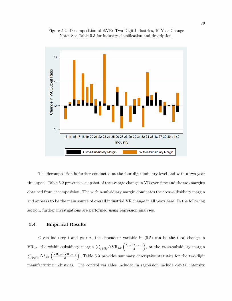
79

Figure 5.2: Decomposition of ∆VR: Two-Digit Industries, 10-Year ChangeNote: See Table 5.3 for industry classification and description.

The decomposition is further conducted at the four-digit industry level and with a two-year

time span. Table 5.2 presents a snapshot of the average change in VR over time and the two margins

obtained from decomposition. The within-subsidiary margin dominates the cross-subsidiary margin

and appears to be the main source of overall industrial VR change in all years here. In the following

section, further investigations are performed using regression analyses.

5.4 Empirical Results

Given industry i and year τ , the dependent variable in (5.5) can be the total change in

VRi,τ , the within-subsidiary margin∑

j∈Ωi∆VRj,τ

(λj,τ+λj,τ−1

2

), or the cross-subsidiary margin∑

j∈Ωi∆λj,τ

(VRj,τ+VRj,τ−1

2

). Table 5.3 provides summary descriptive statistics for the two-digit

manufacturing industries. The control variables included in regression include capital intensity

80

Table 5.2: Change in VR and the Two Margins, Four-digit Industries

Year∆VR Within-Subsidiary Margin Cross-Subsidiary Margin

Mean S.D. Mean S.D. Mean S.D.

1999 0.0116 0.130 0.0119 0.129 -0.00035 0.0188

2000 0.0094 0.112 0.0101 0.111 -0.00071 0.0171

2001 0.0058 0.102 0.0045 0.104 0.00128 0.0145

2002 0.0090 0.111 0.0089 0.110 0.00009 0.0154

2003 0.0093 0.106 0.0111 0.105 -0.00183 0.0151

2004 -0.0084 0.108 -0.0090 0.108 0.00068 0.0184

2005 0.0052 0.106 0.0069 0.104 -0.00164 0.0189

2006 0.0147 0.090 0.0136 0.089 0.00106 0.0150

2007 -0.0043 0.085 -0.0034 0.082 -0.00091 0.0195

(K/L), measured as the value of fixed asset per worker, and the skill intensity indicator, calculated

as the share of employees with the highest completed education equal to or above the level of junior

college. Training intensity, measured as the ratio of employee-training expense to total value of

output, is included to approximate an industry’s learning ability.

81

Table 5.3: Industry Description

Industry code DescriptionCapital Intensity Training intensity Skill Intensity

(K/L)

(1,000 RMB perPerson)

(Employee TrainingExpense/Output)

(Share of Employ-ees with Education≥ Junior College)

13 Processing of Farm and Sideline Food 91.67 0.00028 0.124

14 Manufacture of Food Products 89.07 0.00043 0.138

15 Manufacture of Beverages 149.90 0.00044 0.194

17 Manufacture of Textiles 67.97 0.00035 0.061

18 Manufacture of Wearing Apparel, Footwear, Hats and Caps 23.23 0.00036 0.049

19Manufacture of Leather, Fur, Feather (Down) and RelatedProducts

34.72 0.00030 0.054

20Processing of Wood; Manufacture of Products of Wood,Bamboo, Rattan, Palm Coir and Articles of Straw

74.90 0.00032 0.092

21 Manufacture of Furniture 51.22 0.00040 0.066

22 Manufacture of Paper and Paper Products 116.1 0.00036 0.112

23 Printing and Reproduction of Recorded Media 125.60 0.00069 0.170

24Manufacture of Sport and Recreational Goods (SportsGoods, Toys, Musical Instruments and Stationery Goods)

38.90 0.00038 0.078

25Manufacture of Coke and Refined Petroleum Products;Manufacture of Nuclear Fuel Products

257.00 0.00042 0.202

26 Manufacture of Chemical Material and Chemical Products 161.90 0.00040 0.180

27Manufacture of Pharmaceuticals and Medicinal ChemicalProducts

120.70 0.00061 0.270

28 Manufacture of Chemical Fiber 231.20 0.00026 0.172

29 Manufacture of Rubber Products 70.46 0.00035 0.087

30 Manufacture of Plastics Products 86.59 0.00031 0.093

31 Manufacture of Other Non-metallic Mineral Products 80.47 0.00044 0.102

32 Ferrous Metal Foundries and Presses 193.30 0.00027 0.136

82

Table 5.3 Continued

Industry code DescriptionCapital Intensity Training intensity Skill Intensity

(K/L)

(1,000 RMB perPerson)

(Employee TrainingExpense/Output)

(Share of Employ-ees with Education≥ Junior College)

33 Non-ferrous Metal Foundries and Presses 135.40 0.00029 0.156

34 Manufacture of Fabricated Metal Products (except machinery andequipment)

72.63 0.00044 0.104

35 Manufacture of General Purpose Machinery and Equipment n.e.c. 68.22 0.00054 0.161

36 Manufacture of Special Purpose Machinery 63.73 0.00063 0.195

37 Manufacture of Transport Equipment 89.14 0.00088 0.184

39 Manufacture of Electrical Equipment 74.74 0.00041 0.154

40 Manufacture of Computer and Electronic Products 120.7 0.00034 0.285

41 Manufacture of Special Instruments and Office Machinery 63.38 0.00068 0.252

42 Manufacture of Art Products; Other Manufacturing 45.43 0.00049 0.093

43 Waste Collection, Treatment and Disposal Activities; MaterialsRecovery

92.30 0.00019 0.121

83

Table 5.4 reports the regression results from (5.5) with the overall two-year change in VR at

the four-digit industry level as the dependent variable. Column (1) displays the baseline results,

with only the explanatory variables included. The results are in line with the theory predictions.

VR change is larger when the initial VR is lower; it decreases over time; and it is higher in industries

with higher training intensities. In Column (2), a control variable – capital intensity – is included

into the regression. The results display similar pattern as in the baseline case, and industries with

higher capital intensities tend to show higher growth in VR. Skill intensity is further included as

another control variable with results presented in Column (3). Again, results are consistent with

the theoretical predictions.

Table 5.4: Overall ∆VR of Multinational Operation

(1) (2) (3) (4) (5) (6) (7)

Non

Full Sample Full Sample Full Sample High K/L Low K/L Skill-Intensive Skill-Intensive

Industries Industries Industries Industries

Initial VR -0.0760*** -0.0744*** -0.0743*** -0.0694*** -0.0654*** -0.0711*** -0.0771***

(0.0144) (0.0142) (0.0143) (0.0200) (0.0201) (0.0201) (0.0228)

Year Trend -0.00119* -0.00120** -0.00120** -0.00238*** -0.000046 -0.00200** -0.000454

(τ) (0.000608) (0.000607) (0.000608) (0.000899) (0.000822) (0.000945) (0.000787)

Training 23.32*** 24.30*** 24.54*** 34.92** 16.62** 29.23*** 18.40

Intensity (β) (7.506) (7.345) (7.369) (16.09) (6.706) (9.075) (14.44)

Capital 35.99* 37.57* 43.35** 88.07 26.46 109.6

Intensity (19.57) (20.68) (21.18) (190.4) (21.79) (77.33)

Skill -0.00339 -0.00707 -0.0206 -0.00973 -0.164

Intensity (0.0176) (0.0202) (0.0360) (0.0222) (0.119)

Constant 0.0215*** 0.0176*** 0.0178*** 0.0178* 0.0132 0.0211** 0.0260**

(0.00542) (0.00553) (0.00548) (0.0106) (0.00993) (0.0101) (0.0112)

Observations 2,485 2,485 2,485 1,246 1,239 1,192 1,293

R-squared 0.014 0.015 0.015 0.024 0.012 0.018 0.018

Dependent variable is the two-year change in value-added/output ratio (∆VR).

The regression is at the level of (4-digit industry × year) level. 2-digit industry dummies are included.

Robust standard errors in parentheses.

*** p < 0.01, ** p < 0.05, * p < 0.1

In Columns (4) and (5), VR changes are divided into two groups of industries with high and

low capital-labor intensities, respectively.5 The coefficient of time trend τ is insignificant for the

group of industries with low capital intensities, which confirms that capital-intensive industries tend

5 The groups are defined based on their capital intensities: industries in the high- (low-) intensity group are withcapital-labor intensities above (below) the median of the measure.

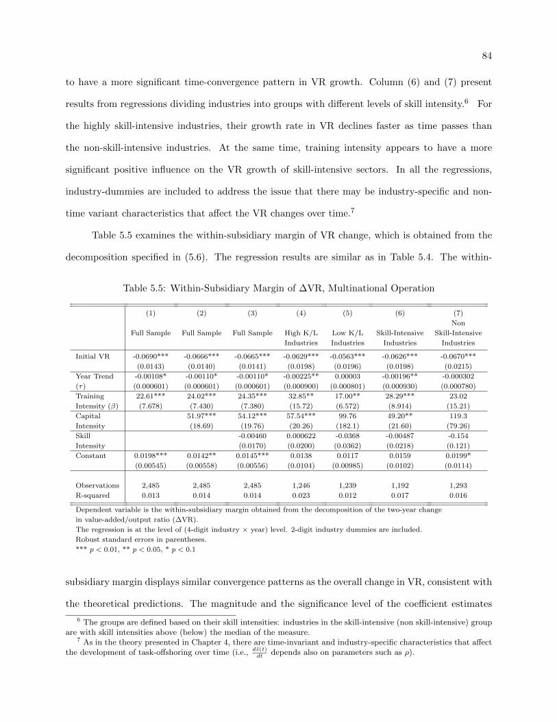
84

to have a more significant time-convergence pattern in VR growth. Column (6) and (7) present

results from regressions dividing industries into groups with different levels of skill intensity.6 For

the highly skill-intensive industries, their growth rate in VR declines faster as time passes than

the non-skill-intensive industries. At the same time, training intensity appears to have a more

significant positive influence on the VR growth of skill-intensive sectors. In all the regressions,

industry-dummies are included to address the issue that there may be industry-specific and non-

time variant characteristics that affect the VR changes over time.7

Table 5.5 examines the within-subsidiary margin of VR change, which is obtained from the

decomposition specified in (5.6). The regression results are similar as in Table 5.4. The within-

Table 5.5: Within-Subsidiary Margin of ∆VR, Multinational Operation

(1) (2) (3) (4) (5) (6) (7)

Non



Initial VR -0.0690*** -0.0666*** -0.0665*** -0.0629*** -0.0563*** -0.0626*** -0.0670***

(0.0143) (0.0140) (0.0141) (0.0198) (0.0196) (0.0198) (0.0215)

Year Trend -0.00108* -0.00110* -0.00110* -0.00225** 0.00003 -0.00196** -0.000302

(τ) (0.000601) (0.000601) (0.000601) (0.000900) (0.000801) (0.000930) (0.000780)

Training 22.61*** 24.02*** 24.35*** 32.85** 17.00** 28.29*** 23.02

Intensity (β) (7.678) (7.430) (7.380) (15.72) (6.572) (8.914) (15.21)

Capital 51.97*** 54.12*** 57.54*** 99.76 49.20** 119.3

Intensity (18.69) (19.76) (20.26) (182.1) (21.60) (79.26)

Skill -0.00460 0.000622 -0.0368 -0.00487 -0.154

Intensity (0.0170) (0.0200) (0.0362) (0.0218) (0.121)

Constant 0.0198*** 0.0142** 0.0145*** 0.0138 0.0117 0.0159 0.0199*

(0.00545) (0.00558) (0.00556) (0.0104) (0.00985) (0.0102) (0.0114)

Observations 2,485 2,485 2,485 1,246 1,239 1,192 1,293

R-squared 0.013 0.014 0.014 0.023 0.012 0.017 0.016

Dependent variable is the within-subsidiary margin obtained from the decomposition of the two-year change

in value-added/output ratio (∆VR).



*** p < 0.01, ** p < 0.05, * p < 0.1

subsidiary margin displays similar convergence patterns as the overall change in VR, consistent with

the theoretical predictions. The magnitude and the significance level of the coefficient estimates

6 The groups are defined based on their skill intensities: industries in the skill-intensive (non skill-intensive) groupare with skill intensities above (below) the median of the measure.

7 As in the theory presented in Chapter 4, there are time-invariant and industry-specific characteristics that affectthe development of task-offshoring over time (i.e., dz(t)

dtdepends also on parameters such as ρ).

85

are quite close to those of overall VR changes, and the convergence patterns are more significant

in highly capital-intensive industries and skill-intensive industries.

Table 5.6 shows the regression results for the cross-subsidiary margin from the decomposition.

With regard to the cross-subsidiary margin, it does not show the similar convergence pattern as

Table 5.6: Cross-Subsidiary Margin of ∆VR, Multinational Operation

(1) (2) (3) (4) (5) (6) (7)

Non



Initial VR -0.00703** -0.00776** -0.00780** -0.00651 -0.00903 -0.00844* -0.0101*

(0.00357) (0.00342) (0.00342) (0.00416) (0.00668) (0.00479) (0.00570)

Year Trend -0.000108 -0.000102 -0.000102 -0.000128 -0.000077 -0.000039 -0.000152

(τ) (0.000129) (0.000128) (0.000128) (0.000196) (0.000167) (0.000190) (0.000176)

Training 0.712 0.278 0.190 2.074 -0.378 0.937 -4.623

Intensity (β) (1.784) (1.728) (1.822) (3.084) (2.809) (1.913) (6.671)

Capital -15.98*** -16.54*** -14.19* -11.69 -22.74*** -9.719

Intensity (5.789) (5.905) (7.214) (47.15) (6.635) (13.94)

Skill 0.00120 -0.00769 0.0162* -0.00486 -0.0102

Intensity (0.00385) (0.00516) (0.00927) (0.00403) (0.0231)

Constant 0.00165 0.00340** 0.00332** 0.00401 0.00154 0.00521** 0.00609**

(0.00126) (0.00140) (0.00141) (0.00267) (0.00267) (0.00254) (0.00255)

Observations 2,485 2,485 2,485 1,246 1,239 1,192 1,293

R-squared 0.011 0.014 0.014 0.017 0.019 0.019 0.028

Dependent variable is the cross-subsidiary margin obtained from the decomposition of the two-year change

in value-added/output ratio (∆VR).



*** p < 0.01, ** p < 0.05, * p < 0.1

of the overall VR change and of the within-subsidiary margin. The cross-subsidiary margin still

decreases in initial VR, while other coefficient estimates of the explanatory variables do not show

the convergence trend. The magnitude, as well as the significance level, of the estimates is much

smaller than those in Table 5.4 and Table 5.5. It is interesting to see that capital intensity tends

to have a negative effect on cross-subsidiary margin, while the effect is positive for both within-

subsidiary margin and the overall VR change. This may imply that the more capital-intensive an

industry is, the more likely it is the case that the VR growth mainly occurs within subsidiaries.

Comparing the results in Table 5.4 – 5.6, it is found that the within-subsidiary change dom-

inates the cross-subsidiary change and serves as the main driving force of the overall convergence

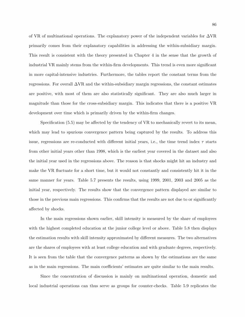
86

of VR of multinational operations. The explanatory power of the independent variables for ∆VR

primarily comes from their explanatory capabilities in addressing the within-subsidiary margin.

This result is consistent with the theory presented in Chapter 4 in the sense that the growth of

industrial VR mainly stems from the within-firm developments. This trend is even more significant

in more capital-intensive industries. Furthermore, the tables report the constant terms from the

regressions. For overall ∆VR and the within-subsidiary margin regressions, the constant estimates

are positive, with most of them are also statistically significant. They are also much larger in

magnitude than those for the cross-subsidiary margin. This indicates that there is a positive VR

development over time which is primarily driven by the within-firm changes.

Specification (5.5) may be affected by the tendency of VR to mechanically revert to its mean,

which may lead to spurious convergence pattern being captured by the results. To address this

issue, regressions are re-conducted with different initial years, i.e., the time trend index τ starts

from other initial years other than 1998, which is the earliest year covered in the dataset and also

the initial year used in the regressions above. The reason is that shocks might hit an industry and

make the VR fluctuate for a short time, but it would not constantly and consistently hit it in the

same manner for years. Table 5.7 presents the results, using 1999, 2001, 2003 and 2005 as the

initial year, respectively. The results show that the convergence pattern displayed are similar to

those in the previous main regressions. This confirms that the results are not due to or significantly

affected by shocks.

In the main regressions shown earlier, skill intensity is measured by the share of employees

with the highest completed education at the junior college level or above. Table 5.8 then displays

the estimation results with skill intensity approximated by different measures. The two alternatives

are the shares of employees with at least college education and with graduate degrees, respectively.

It is seen from the table that the convergence patterns as shown by the estimations are the same

as in the main regressions. The main coefficients’ estimates are quite similar to the main results.

Since the concentration of discussion is mainly on multinational operation, domestic and

local industrial operations can thus serve as groups for counter-checks. Table 5.9 replicates the

87

Table 5.7: ∆VR and its Two Margins, Multinational Operations, Various Initial Years

(1) (2) (3) (4) (5) (6)

Dependent Within-Subsid. Cross-Subsid. Within-Subsid. Cross-Subsid.

Variables ∆VR Margin Margin ∆VR Margin Margin

Initial VR: Year 1999 Initial VR: Year 2001

Initial VR -0.107*** -0.106*** -0.00137 -0.105*** -0.0996*** -0.00507

(0.0160) (0.0157) (0.00338) (0.0227) (0.0220) (0.00526)

Year Trend -0.00112 -0.00102 -0.000100 -0.00206* -0.00198* -0.000081

(τ) (0.000710) (0.000704) (0.000139) (0.00111) (0.00110) (0.00022)

Training 23.93** 25.17** -1.246 20.48* 21.76* -1.285

Intensity (β) (9.697) (9.757) (1.658) (11.98) (12.29) (2.116)

Capital 21.17 35.48 -14.31** -3.462 16.59 -20.05***

Intensity (K/L) (26.35) (24.07) (6.341) (27.81) (26.61) (7.549)

Skill -0.0425 -0.0439* 0.00140 -0.0162 -0.0178 0.00163

Intensity (0.0269) (0.0254) (0.00432) (0.0307) (0.0288) (0.00483)

Constant 0.0350*** 0.0329*** 0.00210 0.0401*** 0.0366*** 0.00351

(0.00709) (0.00699) (0.00143) (0.0105) (0.0106) (0.0022)

R-squared 0.020 0.020 0.013 0.020 0.020 0.013

Initial VR: Year 2003 Initial VR: Year 2005

Initial VR -0.133*** -0.128*** -0.00497 -0.258*** -0.250*** -0.00867

(0.0313) (0.0297) (0.00532) (0.0424) (0.0420) (0.00659)

Year Trend 0.000147 0.000396 -0.000249 -0.0196*** -0.0177*** -0.00195

(τ) (0.00218) (0.00212) (0.000449) (0.00656) (0.00645) (0.00125)

Training 15.17 13.03 2.135 36.61*** 37.82*** -1.217

Intensity (β) (14.88) (15.81) (2.791) (7.839) (7.689) (1.048)

Capital 47.10 57.83* -10.73 -3.093 18.70 -21.79**

Intensity (K/L) (35.39) (31.14) (11.67) (34.89) (34.69) (10.27)

Skill -0.00782 -0.00308 -0.00474 0.0511 0.0417 0.00944

Intensity (0.0329) (0.0313) (0.00682) (0.0373) (0.0376) (0.00661)

Constant 0.0298 0.0259 0.00389 0.224*** 0.204*** 0.0203*

(0.0196) (0.0192) (0.00374) (0.0557) (0.0545) (0.0105)

R-Squared 0.034 0.034 0.019 0.121 0.116 0.036

Specification is the same as column (3) in Tables 5.4 – 5.6.



*** p < 0.01, ** p < 0.05, * p < 0.1

primary regressions on the domestically-funded and the HMT-owned counterparts of MIs. They

are conceptual industries consisting of only domestically-funded and HMT-owned enterprises re-

spectively. The results are quite different from those for multinational operations. The domestic

production does not show a similar convergence pattern, either for the total change in VR or the

within- and cross-firm margins. Particularly, the coefficient estimates on employee training intensity

are negative, which is the opposite of the case of MIs. For HMT-owned operations, the situation

is similar. Except for the initial VR, no other explanatory variable shows significant explanatory

88

Table 5.8: ∆VR and its Two Margins, Multinational Operations, Skill Intensity Measures

(1) (2) (3) (4) (5) (6)

Skill Intensity: Share of Employees Skill Intensity: Share of Employees

with Education ≥ College with Education ≥ Graduate

Dependent Within-Subsid. Cross-Subsid. Within-Subsid. Cross-Subsid.


Initial VR -0.0740*** -0.0662*** -0.00774** -0.0740*** -0.0663*** -0.00770**

(0.0143) (0.0141) (0.00342) (0.0143) (0.0141) (0.00344)

Year Trend -0.00120** -0.00110* -0.000102 -0.00120** -0.00110* -0.000102

(τ) (0.000608) (0.000601) (0.000128) (0.000608) (0.000601) (0.000128)

Training 24.79*** 24.48*** 0.304 24.37*** 24.08*** 0.288

Intensity (β) (7.279) (7.343) (1.751) (7.327) (7.414) (1.727)

Capital 39.81** 55.59*** -15.78*** 36.79* 52.66*** -15.87***

Intensity (K/L) (20.04) (19.00) (5.870) (19.65) (18.74) (5.805)

Skill -0.0183 -0.0173 -0.000971 -0.0518 -0.0446 -0.00721

Intensity (0.0190) (0.0187) (0.00411) (0.0417) (0.0423) (0.0101)

Constant 0.0178*** 0.0144*** 0.00341** 0.0176*** 0.0142** 0.00340**

(0.00548) (0.00555) (0.00140) (0.00553) (0.00558) (0.00139)

R-squared 0.015 0.014 0.014 0.015 0.014 0.014




*** p < 0.01, ** p < 0.05, * p < 0.1

powers. Compared with domestic firms, the HMT-owned production displays patterns closer to the

multinational operations, which may indicate that it is in character more similar to multinational

subsidiaries. For both types of production, it is the within-firm margin that dominates as the main

source of change in overall VR.


The theory of global value chain presented in previous chapters has a key and critical predic-

tion as to how the Southern host country’s share of industrial value added behaves over time: its

dynamics essentially follows a convergence pattern similar to the evolution path of the offshoring

threshold. The VR of a multinational industry in a Southern host country will grow at a decreasing

speed, as predicted. Using subsidiary-level data on Chinese multinational operations, the prediction

is empirically investigated in this chapter.

The empirical results show evidence supporting the theoretical predictions. The multinational

89

Table 5.9: ∆VR and its Two Margins, Local Production and HMT-Owned Operations

(1) (2) (3) (4) (5) (6)

Domestically-Funded Production HMT-Owned Production

Dependent Within-Firm Cross-Firm Within-Firm Cross-Firm


Initial VR -0.0279** -0.0205 -0.00739* -0.0873*** -0.0849*** -0.00240

(0.0141) (0.0151) (0.00438) (0.0129) (0.0121) (0.00408)

Year Trend 0.0000995 -0.000159 0.000258*** 0.000926 0.000743 0.000183

(τ) (0.000211) (0.000203) (0.0000596) (0.000661) (0.000658) (0.000137)

Training -13.54** -12.41* -1.135 3.119 3.938 -0.819

Intensity (β) (5.898) (6.349) (0.773) (6.773) (6.401) (1.852)

Capital -10.89 -10.14 -0.749 -33.25 -39.21 5.960

Intensity (K/L) (10.65) (8.999) (4.355) (32.22) (32.88) (5.808)

Skill 0.0178** 0.0198** -0.00200 0.0596*** 0.0615*** -0.00186

Intensity (0.00813) (0.00773) (0.00256) (0.0216) (0.0219) (0.00537)

Constant 0.0125*** 0.0103*** 0.00225 0.0149*** 0.0150*** -0.0000722

(0.00341) (0.00370) (0.00142) (0.00537) (0.00527) (0.00121)

Observations 3,777 3,777 3,777 2,521 2,521 2,521

R-squared 0.021 0.021 0.019 0.021 0.022 0.008




*** p < 0.01, ** p < 0.05, * p < 0.1

subsidiaries in China experience VR growth during the time period covered in the dataset, at a

declining pace. The employee training intensity of an industry has a significant positive effect on VR

growth. The results are robust to different choices of initial years and control variables’ measures.

A similar convergence pattern is not found when I perform regression using the same specification

on domestic and HMT-owned operations. Certainly, it is ideal that the empirical investigation is

performed at the task level, i.e., the observations are tasks conducted within subsidiaries. While

task-level data are difficult to obtain and not widely available, in this chapter firm-level data are

examined to the best exertion.

Chapter 6

An Extenstion: Multinational Production, Innovation, and

the Dynamics of Task Allocation

In the basic model presented in Chapter 3, the technologically advanced country serves as the

learning boundary, which does not change over time. Recently, there is a rising phenomenon catch-

ing people’s attention – “reshoring,” which refers to the trend that previously offshored activities

are now moved back to their originating home countries. One important driving force behind this

occurrence is that the technologically developed home countries improve their production efficiency

over time, which gradually makes it more economic to conduct even the low-end activities back

there. Therefore, this chapter considers the task-allocation dynamics in global production with

technology innovation in the North incorporated.

In this theoretical extension of the basic model, while the South learns by carrying out tasks

beyond its capability, the North keeps innovating. The technologies in the developed country keep

being improved – the technology frontier and learning boundary of the world keeps being pushed

forward. The task allocation pattern at any point of time depends on countries’ relative cost of

conducting each activity. The dynamics of global production are thus critically determined by

the two countries’ relative speed of technology improvement – one through learning and the other

through innovation. Under this framework, both offshoring expansion and reshoring may occur.

This chapter mainly discusses the task-allocation dynamics under different circumstances

of technology improvement interaction between countries. It is organized as follows. In Section

6.1, I introduce the environment and set-up of the model. Section 6.2 studies the instantaneous

91

equilibrium of multinational production. The dynamics of task allocation are discussed in Section

6.3 and 6.4, for an initially efficient and inefficient South, respectively. Section 6.5 concludes.


The environment is the same as in the basic model introduced in Chapter 3. There are two

countries: North (N) and South (S), with one industry producing a final product Y and supplying

it to both countries’ consumers, with no trade cost. Consumer preferences are the same in the

two countries. Labor is the only factor of production, which is inelastically supplied and immobile

across countries. The labor endowment of country i is denoted by Li, and it is constant over time.

Time is continuous and indexed by t. The environment is perfectly competitive.

6.1.1 Production

As in the basic model, the production of Y requires the completion of a continuum of tasks,

indexed by z ∈ [0, 1]. The value of z indicates the technological sophistication of a task. The

production function of Y at any time t is expressed as:

lnY (t) =

∫ 1

0lnx(z, t)dz, (6.1)

where x(z, t) is the amount of task z completed at time t. Each task can be carried out in either

country with constant returns to scale.

Initially at t = 0, the North can perform any task with the best technology available at that

time. The unit labor requirement for conducting a task z in the North at t = 0 is given by

aN (z, 0) = ae−z, (6.2)

where a > 0 is a parameter. The South, in contrast, has the best technology in use initially only

for some low-sophistication tasks. Specifically, let T (0) denote the efficiency frontier of technology

in the South at t = 0, with 0 < T (0) < 1. For the simple tasks with z ≤ T (0), the South’s

production technologies are as good as the North’s. For the complicated ones with z > T (0), the

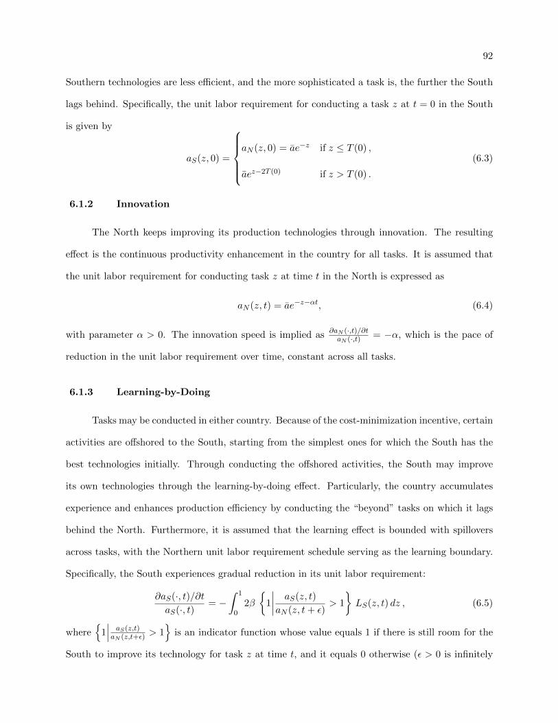
92

Southern technologies are less efficient, and the more sophisticated a task is, the further the South

lags behind. Specifically, the unit labor requirement for conducting a task z at t = 0 in the South

is given by

aS(z, 0) =

aN (z, 0) = ae−z if z ≤ T (0) ,

aez−2T (0) if z > T (0) .

(6.3)

6.1.2 Innovation

The North keeps improving its production technologies through innovation. The resulting

effect is the continuous productivity enhancement in the country for all tasks. It is assumed that

the unit labor requirement for conducting task z at time t in the North is expressed as

aN (z, t) = ae−z−αt, (6.4)

with parameter α > 0. The innovation speed is implied as ∂aN (·,t)/∂taN (·,t) = −α, which is the pace of

reduction in the unit labor requirement over time, constant across all tasks.


Tasks may be conducted in either country. Because of the cost-minimization incentive, certain

activities are offshored to the South, starting from the simplest ones for which the South has the

best technologies initially. Through conducting the offshored activities, the South may improve

its own technologies through the learning-by-doing effect. Particularly, the country accumulates

experience and enhances production efficiency by conducting the “beyond” tasks on which it lags

behind the North. Furthermore, it is assumed that the learning effect is bounded with spillovers

across tasks, with the Northern unit labor requirement schedule serving as the learning boundary.

Specifically, the South experiences gradual reduction in its unit labor requirement:

∂aS(·, t)/∂taS(·, t)

= −∫ 1

02β

1

∣∣∣∣ aS(z, t)

aN (z, t+ ε)> 1

LS(z, t) dz , (6.5)

where

1∣∣∣ aS(z,t)aN (z,t+ε) > 1

is an indicator function whose value equals 1 if there is still room for the

South to improve its technology for task z at time t, and it equals 0 otherwise (ε > 0 is infinitely

93

small); LS(z, t) denotes the amount of labor used for carrying out task z in the South at time t;

and β > 0 is a parameter implying the learning ability of the South. The basic idea is that while

the North keeps improving technologies for every task, the world’s production efficiency frontier

continues moving forward, which may lead the South to keep trying catching up with the North.

At the same time, the learning effect has a boundary. It is assumed that the North always

has the best technologies, and the South is not able to achieve better than the North at any time.

Hence, the Northern efficiency function always serves as the boundary of Southern learning.

Examining the learning function (6.5), it is found that with the constant Northern technology

improvement, the Southern learning effect is essentially given by

∂aS(·, t)/∂taS(·, t)

= −∫ 1

02β × 1 × LS(z, t) dz = −2βLS , (6.5′)

when aS(z, t) ≥ aN (z, t), and if the South does conduct some tasks at time t. Intuitively, while

the North keeps innovating on all technologies, the South only learns from the North. As a result,

there always exists room for the South to learn the most up-to-date technologies. The learning

effect reveals the possibility that a host country may improve its own technologies constantly by

conducting offshored tasks, and all resources devoted contribute to technology improvement.

With Northern innovation and Southern learning, the pattern of how the productivity sched-

ules may evolve over time depends on the interaction between the two. There are three possible

cases with regard to the relationship between innovation and learning:

• Case I. Northern Innovation Pace = Southern Learning Pace (α = 2βLS)

• Case II. Northern Innovation Pace > Southern Learning Pace (α > 2βLS)

• Case III. Northern Innovation Pace < Southern Learning Pace (α < 2βLS)

The dynamics of task allocation vary upon different circumstances. I will examine each case in

detail in later discussions.

All tasks, wherever allocated, are conducted using the local unit labor requirement schedules.

In this model with perfectly competitive environment, tasks are undertaken with constant returns

94

to scale. Therefore, firms do not have a substantial role here from the theoretical perspective.

6.2 Instantaneous Equilibrium of Multinational Production


Let wi(t) denote the wage rate in coutry i at time t. The unit cost functions for conducting

a task z in the two countries are, respectively,

CS(wS(t), z) = wS(t)aS(z, t) , (6.6)

CN (wN (t), z) = wN (t)aN (z, t) . (6.7)

A certain range of tasks are offshored to the South, starting from the simplest ones, since the South

has the most advanced technologies for them initially. The cost conditions (6.6) and (6.7) combine

to form a no-arbitrage condition of offshoring, determining the pattern of task allocation between

countries. There exists a threshold task z(t) at time t such that CS(wS(t), z) = CN (wN (t), z) in

equilibrium, i.e.,

wS(t) aS(z(t), t) = wN (t) aN (z(t), t) , (6.8)

where z(t) > 0 is the most sophisticated task that is performed in the South. The tasks beyond

z(t) are conducted in the North.

The labor-market clearing conditions in the two countries at time t are:

South :

∫ z(t)

0xS(z, t)aS(z, t)dz = LS , (6.9)

North :

∫ 1

z(t)xN (z, t)aN (z, t)dz = LN , (6.10)

where xi(z, t) denotes the amount of task z conducted in country i at time t.

Similar as in Chapter 3, let E(t) denote the world expenditure on the final consumer product

Y at time t, defined as the sum of factor payments in the two economies:

E(t) = wS(t)LS + wN (t)LN . (6.11)

95

Then the demand for a task z conducted in country i at time t is

xi(z, t) =E(t)

Ci(wi(t), z), i ∈ N,S . (6.12)

With the unit cost functions (6.6) and (6.7), together with (6.12), the labor-market clearing condi-

tions are simplified to

South :

∫ z(t)

0

E(t)

wS(t)dz = LS , (6.9′)

North :

∫ 1

z(t)

E(t)

wN (t)dz = LN . (6.10′)

Therefore, the instantaneous equilibrium at any time t is characterized by the offshoring

threshold determination condition (6.8), the labor-market clearing conditions (6.9′) and (6.10′),

and the world expenditure expression (6.11). I normalize world expenditure at unity by Walras’

Law: E(t) = 1, and hereby wage rates are thus measured as shares of world factor income.

6.2.2 The Wage-Equalization Threshold

There exists a threshold task z∗, such that if all tasks with z ∈ [0, z∗] are offshored to the

South, and all tasks with z ∈ (z∗, 1] are conducted in the North, the two countries’ wage rates are

equalized. From conditions (6.9′) and (6.10′), this wage-equalization threshold task z∗ is

z∗ =LS

LS + LN. (6.13)

This wage-equalization threshold task z∗ is critical for analyzing the equilibrium dynamics.

On one hand, it determines whether the host country receives “beyond” tasks to conduct when

offshoring begins. If it is lower than the initial Southern technology stock (z∗ < T (0)), the North

will not offshore more than z∗ (thus no more than T (0)) tasks to the South. However, if z∗ > T (0),

the North may offshore more than T (0) tasks, and thus the South conducts activities that it is not

good at, at the initial time. On the other hand, the position of z∗ significantly influences how task

allocation evolves over time. My discussion thus will proceed with two possible cases:

• Case I. The South is relatively efficient initially: z∗ ≤ T (0);

• Case II. The South is relatively inefficient initially: z∗ > T (0).

96

6.3 The Evolution Dynamics: An Initially Efficient South

This is the case where the South is relatively capable in terms of production efficiency:

z∗ ≤ T (0). In this situation, all low-sophistication tasks below z∗ will be offshored to the South

initially. All tasks thus are conducted using the best available technologies. The initial equilibrium

is characterized by the following:

wS(0) ae−z(0) = wN (0) ae−z(0) , (6.14)∫ z(0)

0

1

wS(0)dz = LS , (6.15)∫ 1

z(0)

1

wN (0)dz = LN . (6.16)

Given the conditions, the task threshold of offshoring z(0) and wage rates are given by, respectively,

z(0) = z∗ =LS

LS + LN, (6.17)

wS(0) = wN (0) = w∗ =1

LS + LN. (6.18)

6.3.1 Evolution Dynamics: Equal Paces of Technological Progress

When the technological progresses in the two countries are at the same pace (α = 2βLS),

the efficiency gap between the two countries’ technologies will not be changing over time. With the

learning function (6.5′), at any time t, the Southern unit labor requirement schedule is given by

aS(z, t) =

aN (z, t) = ae−z−αt if z ≤ T (0) ,

aez−2T (0)−αt if z > T (0) .

(6.19)

This indicates that the relative efficiency of conducting tasks is:

aS(z, t)

aN (z, t)=

1 if z ≤ T (0) ,

e2z−2T (0) if z > T (0) ,

(6.20)

which keeps the same over time.

Given the fact the relative efficiency schedule does not change, the task allocation pattern

also stays the same as initially. When both countries are improving their technologies at the same

97

pace, the countries’ comparative advantages in terms of task-conduct do not change, which leads

to an overall static equilibrium in this case:

z(t) = z∗ =LS

LS + LN, (6.21)

wS(t) = wN (t) = w∗ =1

LS + LN. (6.22)

Figure 6.1 shows this situation graphically.

Figure 6.1: Dynamics of Task Offshoring: an Initially Efficient South, Equal Paces ofTechnological Progress (z∗ ≤ T (0), α = 2βLS)

0 1


z

North at t=0

South at t=0

South at t>0

North at t>0

T(t) = T(0)z(t) = z*

6.3.2 Evolution Dynamics: Fast Northern Innovation

This is the situation where the initially technologically developed country pushes the world’s

technology frontier faster than the Southern learning pace: α > 2βLS . Therefore, the Southern

learning under this circumstance will not be bounded – the South will not be able to catch up with

the North. Specifically, the unit labor requirement schedule of the South is:

aS(z, t) =

ae−z−2βLSt if z ≤ T (0) ,

aez−2T (0)−2βLSt if z > T (0) .

(6.23)

98

The technological difference between the countries becomes increasingly significant over time:

aS(z, t)

aN (z, t)=

e(α−2βLS)t if z ≤ T (0) ,

e2z−2T (0)+(α−2βLS)t if z > T (0) .

(6.24)

Reshoring Behavior With the productivity schedules, the conditions for instantaneous

equilibrium (6.8), (6.9′) and (6.10′) after the initial time period boil down to

e(α−2βLS)t =1− z(t)z(t)

× LSLN

, (6.25)

wS(t) =z(t)

LS, (6.26)

wN (t) =1− z(t)LN

. (6.27)

Comparing the two task-threshold determination functions at t = 0 vs. t > 0 ((6.17) vs. (6.25)), it

is easy to find that with fast Northern innovation, at any t > 0, it is the case that less than z∗ tasks

are offshored: z(t) < z(0) = z∗. Here a potential assumption is that task allocation is sticky: the

progress of offshoring keeps the set of tasks offshored as close as that in the previous time period.

This is consistent with the common observations in real business, where sharp and significant shifts

of the offshoring pattern seldom occur.

Therefore, with the widening of the technological gap between countries, fewer than z(0) tasks

are allocated to the South. Productivity growth arising from innovation alleviates the reliance of

multinational production on the South for production. Over time, with both Southern learning

and Northern innovation, global production evolves. Particularly, while the South lags increasingly

further behind, the Southern coverage of tasks shrinks, including fewer sophisticated tasks. This

can been seen by examining (6.25):1

dz(t)

dt< 0 , (6.28)

The task offshoring threshold gradually lowers over time. After initial offshoring, with fast

Northern innovation, tasks that were originally offshored are moved back to the North, starting

1 From (6.25), z(t) = LSLS+LNe

(α−2βLS)t , which monotonically decreases in t with α > 2βLS .

99

from those relatively sophisticated ones. The “reshoring” trend thus occurs. This can be seen

graphically in Figure 6.2.

Figure 6.2: Dynamics of Task Offshoring: an Initially Efficient South, Fast Northern Innovation(z∗ ≤ T (0), α > 2βLS)

0 1


z

North at t=0

South at t=0

South at t>0

North at t>0

T(0)z(t) z(0)z*

How fast the reshoring behavior will proceed depends on the two countries’ difference in their

domestic paces of technology progress. From (6.25), it is found that a constant threshold, 12 , serves

as the threshold of sign-change of d2z(t)dt2

. When more than half of the tasks are offshored to the

South, the reshoring speed is increasingly fast; when less than half of the tasks are offshored, the

reshoring speed decreases. In functional form, it can be expressed as:2

d2z(t)

dt2

< 0 when z(t) > 12 ,

= 0 when z(t) = 12 ,

> 0 when z(t) < 12 .

(6.29)

Over time, the offshoring threshold converges to: limt→+∞ z(t) = 0. Certainly, the threshold

z(t) will not really touch 0, and the progress mainly indicates that the range of tasks that are

offshored will be shrinking over time, with the South increasingly only focusing on the simplest

2 See Appendix C.1 for the derivation.

100

activities. Figure 6.3 illustrates two possible evolution paths of the reshoring behavior. In Panel

A, the initial threshold z(0) = z∗ is above 12 . Given the definition of z∗, (6.13), this situation

essentially indicates a large South: LS > LN . Therefore, this evolution pattern is likely to occur

when the South is both large and initially efficient. In Panel B, offshoring starts with z(0) < 12 ,

which is likely to be case when the South is relatively small: LS < LN . This story illustrates

Figure 6.3: Evolution of Offshoring Threshold: An Initially Efficient South, Fast NorthernInnovation (z∗ ≤ T (0), α > 2βLS)

(a) Panel A: A Relatively Large South: 12 < z∗ ≤ T (0)

0

z(t)

t

z*

1/2

(b) Panel A: A Relatively Small South: z∗ < 12

0

z(t)

t

z*

1/2

101

that with technology progressing faster in the home country, the learning effect in the South is not

adequate to enable the host country to receive more tasks to conduct. It is the relative technology

advantage/disadvantage that determines the offshoring pattern.

6.3.3 Evolution Dynamics: Fast Southern Learning

With fast Southern learning (2βLS > α), the technological gap between the two economies

closes over time – the host country catches up with the home country gradually. It is assumed

that during this process, the Northern schedule serves as the learning boundary. The Southern

technologies do not get better than the corresponding Northern ones at any point of time. After

the initial time period, considering the productivity schedules (6.3) and (6.4), and learning function

(6.5′), together with the condition α < 2βLS , the unit labor requirement in the South is given by

aS(z, t) =

aN (z, t) = ae−z−αt if z ≤ T (t) = T (0) + (βLS − α

2 )t ,

aez−2T (0)−2βLSt if z > T (t) = T (0) + (βLS − α2 )t .

(6.30)

It thus is the case that the Southern stock of technology (T (t)) moves towards more sophisticated

tasks over time, i.e., the South is getting the most advanced technologies for increasingly more

difficult tasks. The technological gap between countries gradually diminishes:

aS(z, t)

aN (z, t)=

1 if z ≤ T (t) = T (0) + (βLS − α

2 )t ,

e2z−2T (0)+(α−2βLS)t if z > T (t) = T (0) + (βLS − α2 )t .

(6.31)

It is obvious that countries’ efficiency gap of conducting all tasks will be closing over time, with

faster Southern learning, 2βLS > α.

While the technology stock in the South, T (t), shifts to the right, it thus is the case that

z∗ ≤ T (0) < T (t) when t > 0. Therefore, following the same logic as when discussing the initial

equilibrium at the beginning of this section, it is easy to tell that under this situation, z(t) = z(0) =

z∗. No more than z∗ tasks will be offshored as it will not be cost-minimizing, even if the South

has increasingly better technologies. The reason is that although the South learns faster than the

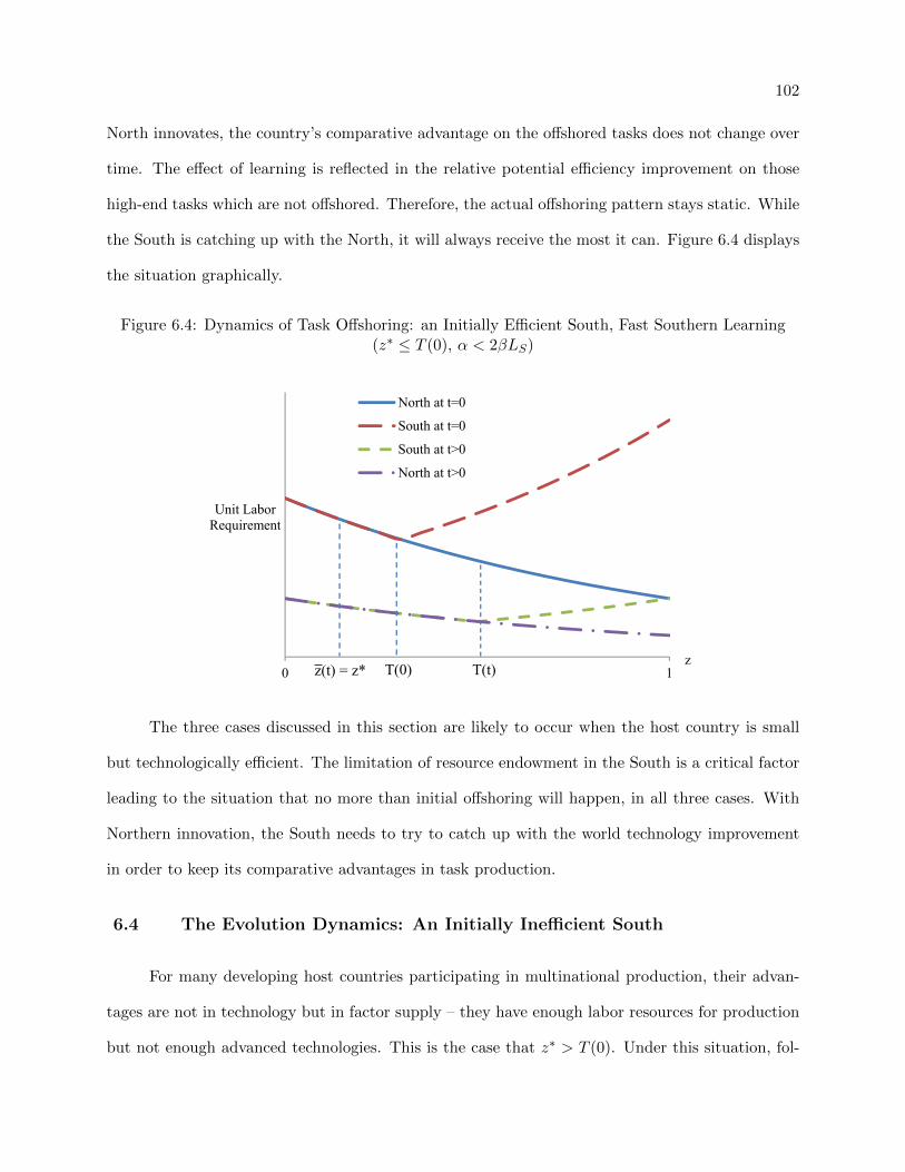
102

North innovates, the country’s comparative advantage on the offshored tasks does not change over

time. The effect of learning is reflected in the relative potential efficiency improvement on those

high-end tasks which are not offshored. Therefore, the actual offshoring pattern stays static. While

the South is catching up with the North, it will always receive the most it can. Figure 6.4 displays

the situation graphically.

Figure 6.4: Dynamics of Task Offshoring: an Initially Efficient South, Fast Southern Learning(z∗ ≤ T (0), α < 2βLS)

0 1


z

North at t=0

South at t=0

South at t>0

North at t>0

T(0) T(t)z(t) = z*

The three cases discussed in this section are likely to occur when the host country is small

but technologically efficient. The limitation of resource endowment in the South is a critical factor

leading to the situation that no more than initial offshoring will happen, in all three cases. With

Northern innovation, the South needs to try to catch up with the world technology improvement

in order to keep its comparative advantages in task production.

6.4 The Evolution Dynamics: An Initially Inefficient South

For many developing host countries participating in multinational production, their advan-

tages are not in technology but in factor supply – they have enough labor resources for production

but not enough advanced technologies. This is the case that z∗ > T (0). Under this situation, fol-

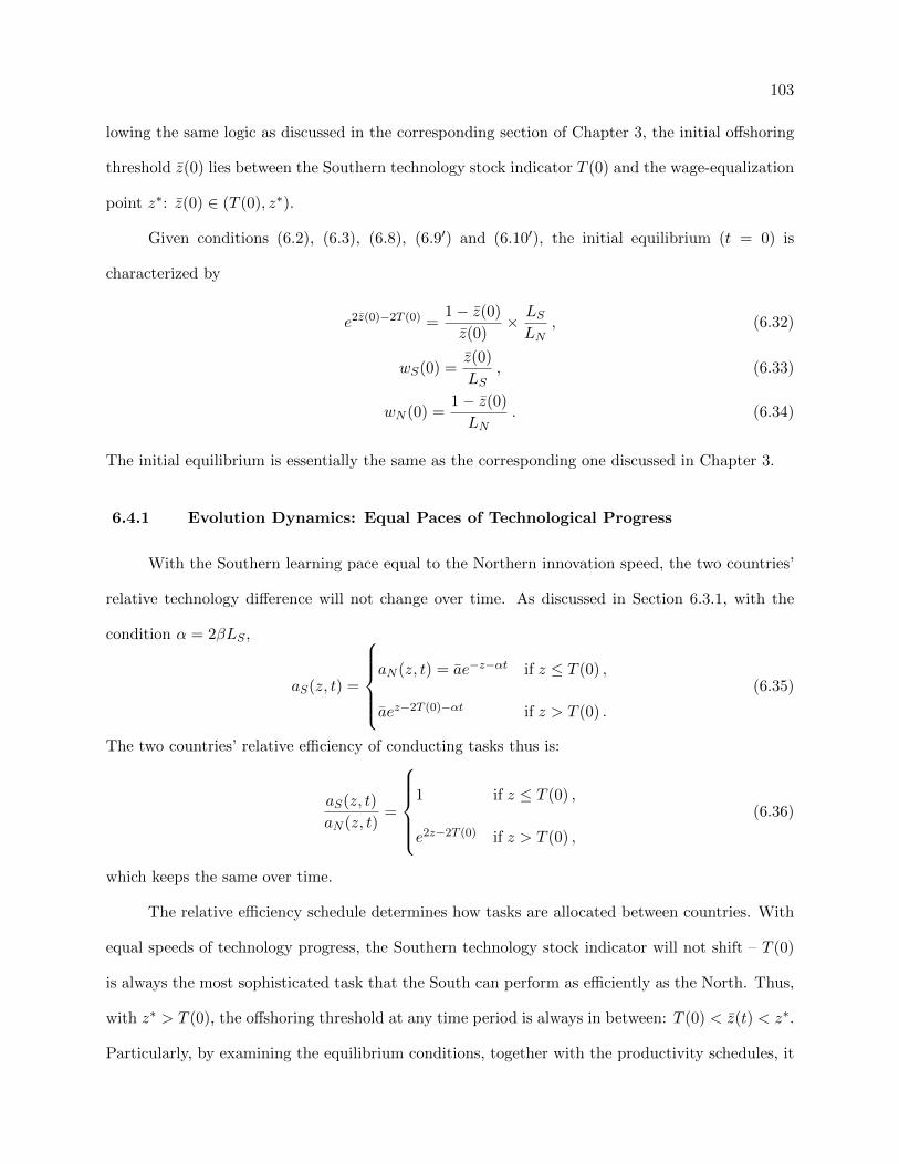
103

lowing the same logic as discussed in the corresponding section of Chapter 3, the initial offshoring

threshold z(0) lies between the Southern technology stock indicator T (0) and the wage-equalization

point z∗: z(0) ∈ (T (0), z∗).

Given conditions (6.2), (6.3), (6.8), (6.9′) and (6.10′), the initial equilibrium (t = 0) is

characterized by

e2z(0)−2T (0) =1− z(0)

z(0)× LSLN

, (6.32)

wS(0) =z(0)

LS, (6.33)

wN (0) =1− z(0)

LN. (6.34)

The initial equilibrium is essentially the same as the corresponding one discussed in Chapter 3.

6.4.1 Evolution Dynamics: Equal Paces of Technological Progress

With the Southern learning pace equal to the Northern innovation speed, the two countries’

relative technology difference will not change over time. As discussed in Section 6.3.1, with the

condition α = 2βLS ,

aS(z, t) =

aN (z, t) = ae−z−αt if z ≤ T (0) ,

aez−2T (0)−αt if z > T (0) .

(6.35)

The two countries’ relative efficiency of conducting tasks thus is:

aS(z, t)

aN (z, t)=

1 if z ≤ T (0) ,

e2z−2T (0) if z > T (0) ,

(6.36)

which keeps the same over time.

The relative efficiency schedule determines how tasks are allocated between countries. With

equal speeds of technology progress, the Southern technology stock indicator will not shift – T (0)

is always the most sophisticated task that the South can perform as efficiently as the North. Thus,

with z∗ > T (0), the offshoring threshold at any time period is always in between: T (0) < z(t) < z∗.

Particularly, by examining the equilibrium conditions, together with the productivity schedules, it

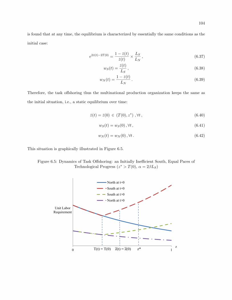
104

is found that at any time, the equilibrium is characterized by essentially the same conditions as the

initial case:

e2z(t)−2T (0) =1− z(t)z(t)

× LSLN

, (6.37)

wS(t) =z(t)

LS, (6.38)

wN (t) =1− z(t)LN

. (6.39)

Therefore, the task offshoring thus the multinational production organization keeps the same as

the initial situation, i.e., a static equilibrium over time:

z(t) = z(0) ∈ (T (0), z∗) , ∀t , (6.40)

wS(t) = wS(0) ,∀t , (6.41)

wN (t) = wN (0) ,∀t . (6.42)

This situation is graphically illustrated in Figure 6.5.

Figure 6.5: Dynamics of Task Offshoring: an Initially Inefficient South, Equal Paces ofTechnological Progress (z∗ > T (0), α = 2βLS)

0 1


z

North at t=0

South at t=0

South at t>0

North at t>0

T(t) = T(0) z*z(t) = z(0)

105

6.4.2 Evolution Dynamics: Fast Northern Innovation

As discussed earlier in the chapter, when the North is able to push the world technology

frontier faster than the South can catch up (α > 2βLS), the efficiency gap between countries

widens over time. The developing country will be increasingly lagging behind, although it is also

improving. At t > 0, the unit labor requirement schedule of the South is:

aS(z, t) =

ae−z−2βLSt if z ≤ T (0) ,

aez−2T (0)−2βLSt if z > T (0) .

(6.43)

The technological gap between the countries widens over time:

aS(z, t)

aN (z, t)=

e(α−2βLS)t if z ≤ T (0) ,

e2z−2T (0)+(α−2βLS)t if z > T (0) .

(6.44)

After the countries start establishing the multinational production chain at t = 0, within a

certain time period, the offshoring threshold z(t) is still within the interval (T (0), z∗). During this

time period, the equilibrium is characterized by

e2z(t)−2T (0)+(α−2βLS)t =1− z(t)z(t)

× LSLN

, (6.45)

wS(t) =z(t)

LS, (6.46)

wN (t) =1− z(t)LN

. (6.47)

Comparing the task threshold determination conditions at t > 0 vs. at t = 0 ((6.45) vs. (6.32)),

together with the condition that α > 2βLS , it is easy to tell that the offshoring threshold in the

following time period, z(t), shifts towards less-sophisticated tasks: z(t) < z(0). Therefore, with

the increasingly wide technological gap between countries, multinationals tend to move previously

offshored tasks back to the home country. Although during the process, the wage rate in the South

is always lower than in the North (wS(t) < wN (t))3 , reshoring behavior still occurs. The developing

country’s labor cost advantage is not adequate to attract more offshoring. In contrast, although it

3 This can be told by comparing (6.46) and (6.47), together with the condition that z(t) < z∗ = LSLS+LN

.

106

costs higher in the developed country to hire workers, the technology advantage there attracts more

activities to return. Anecdotal evidence has shown that multinational firms invest in reshoring in

recent years, even though host countries’ unit labor costs are lower than home countries’. Such

stories and observations are consistent with the analysis presented here – with better technologies

and continuous improvement, the developed countries may enjoy more manufacturing activities

being relocated back.

After a certain time period, the offshoring threshold z(t) moves down to T (0). After that, as

the efficiency gap between the countries continues widening, the reshoring behavior will continue.

That is, the South starts only conducting the tasks that it is relatively good at. The first condition

characterizing the equilibrium – the threshold determination condition – thus changes to:

e(α−2βLS)t =1− z(t)z(t)

× LSLN

. (6.48)

As time passes, with high innovation pace in the North, the scope of tasks that are conducted in

the South shrinks. During the whole process, reshoring persists. The situation can be graphically

shown in Figure 6.6.

Figure 6.6: Dynamics of Task Offshoring: an Initially Inefficient South, Fast Northern Innovation(z∗ > T (0), α > 2βLS)

0 1


z

North at t=0

South at t=0

South at t>0

North at t>0

T(t) = T(0) z(t) z(0) z*

107

Reshoring Behavior Examining the reshoring behavior in the two stages respectively, it

is found that before the offshoring threshold goes below T (0), the following pattern applies:4

dz(t)

dt

∣∣∣∣T (0)≤z(t)<z∗

= −(α− 2βLS)× z(t) (1− z(t))1 + 2z(t) (1− z(t))

< 0 , (6.49)

d2z(t)

dt2

∣∣∣∣T (0)≤z(t)<z∗

< 0 when z(t) > 12 ,

= 0 when z(t) = 12 ,

> 0 when z(t) < 12 .

(6.50)

After the offshoring threshold goes below T (0), the situation will follow a similar pattern as dis-

cussed in Section 6.3.2, where the offshoring threshold is below the initial technology stock in the

South, T (0), with the Northern innovation speed faster than that in the South. Technically, this

can be seen by comparing the equilibrium conditions (6.48) and (6.25). Therefore, following the

same logic, in this stage, the reshoring behavior is characterized by

dz(t)

dt

∣∣∣∣z(t)≤T (0)<z∗

< 0 , (6.51)

d2z(t)

dt2

∣∣∣∣z(t)≤T (0)<z∗

< 0 when z(t) > 12 ,

= 0 when z(t) = 12 ,

> 0 when z(t) < 12 .

(6.52)

At z(t) = T (0), dz(t)dt is not continuous.5 When time goes infinite, the technology gap also goes

infinite, which leads to limt→+∞ z(t) = 0.

Figure 6.7 displays a couple possible evolution paths of the reshoring behavior for a relatively

large South: LS > LN thus z∗ > 12 . Panel A shows the case where the South has a relatively large

technology stock at the beginning: 12 < T (0) < z∗. In Panel B, the initial stock of technology in

the South is relatively small: T (0) < 12 < z(0) < z∗. In Figure 6.8, the South is relatively small in

terms of labor endowment: LS < LN . Therefore, the wage equalization point z∗ < 12 .

4 The expression for dz(t)dt

is from examining (6.45). See Appendix C.2.1 for the derivation of d2z(t)

dt2.

5 From (6.49), dz(t)dt|−z(t)=T (0) = − (α−2βLS)×T (0)(1−T (0))

1+2T (0)(1−T (0)); From (6.48), dz(t)

dt|+z(t)=T (0) = −(α−2βLS)T (0)(1−T (0)).

Therefore, dz(t)dt|−z(t)=T (0) >

dz(t)dt|+z(t)=T (0).

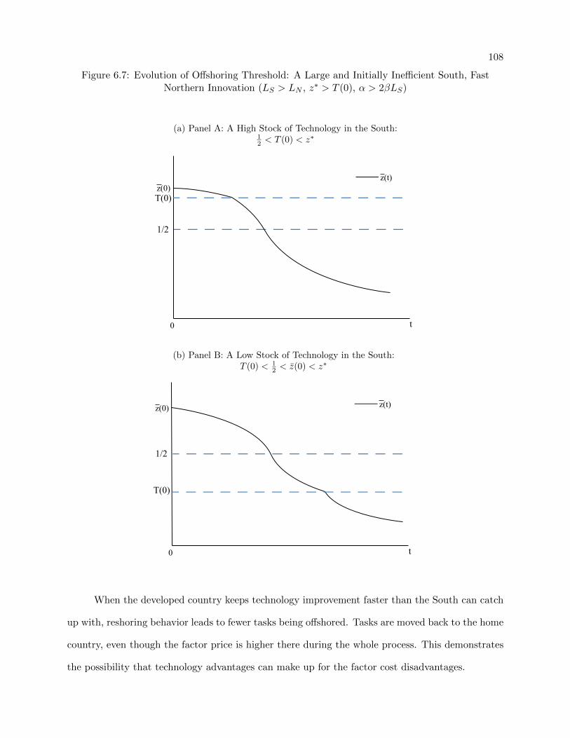
108

Figure 6.7: Evolution of Offshoring Threshold: A Large and Initially Inefficient South, FastNorthern Innovation (LS > LN , z∗ > T (0), α > 2βLS)

(a) Panel A: A High Stock of Technology in the South:12 < T (0) < z∗

0

z(t)

t

1/2

T(0)z(0)

(b) Panel B: A Low Stock of Technology in the South:T (0) < 1

2 < z(0) < z∗

0

z(t)

t

1/2

T(0)

z(0)

When the developed country keeps technology improvement faster than the South can catch

up with, reshoring behavior leads to fewer tasks being offshored. Tasks are moved back to the home

country, even though the factor price is higher there during the whole process. This demonstrates

the possibility that technology advantages can make up for the factor cost disadvantages.

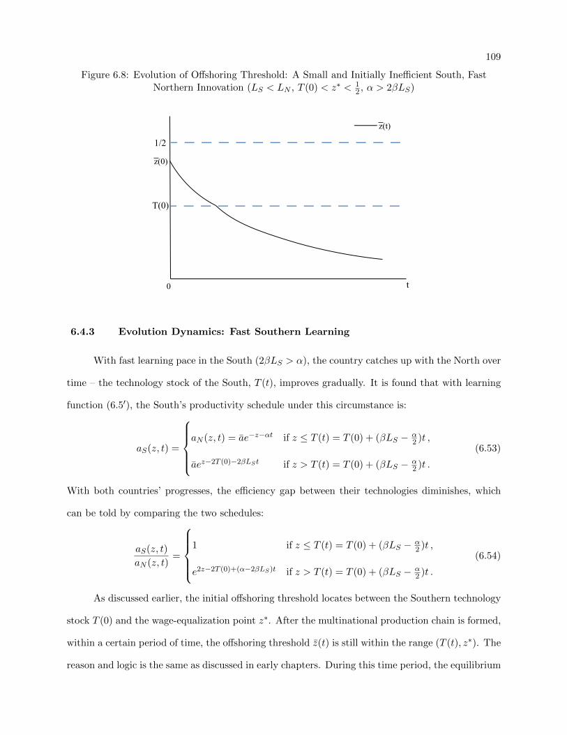
109

Figure 6.8: Evolution of Offshoring Threshold: A Small and Initially Inefficient South, FastNorthern Innovation (LS < LN , T (0) < z∗ < 1

2 , α > 2βLS)

0

z(t)

t

1/2

T(0)

z(0)

6.4.3 Evolution Dynamics: Fast Southern Learning

With fast learning pace in the South (2βLS > α), the country catches up with the North over

time – the technology stock of the South, T (t), improves gradually. It is found that with learning

function (6.5′), the South’s productivity schedule under this circumstance is:

aS(z, t) =

aN (z, t) = ae−z−αt if z ≤ T (t) = T (0) + (βLS − α

2 )t ,

aez−2T (0)−2βLSt if z > T (t) = T (0) + (βLS − α2 )t .

(6.53)

With both countries’ progresses, the efficiency gap between their technologies diminishes, which

can be told by comparing the two schedules:

aS(z, t)

aN (z, t)=

1 if z ≤ T (t) = T (0) + (βLS − α

2 )t ,

e2z−2T (0)+(α−2βLS)t if z > T (t) = T (0) + (βLS − α2 )t .

(6.54)

As discussed earlier, the initial offshoring threshold locates between the Southern technology

stock T (0) and the wage-equalization point z∗. After the multinational production chain is formed,

within a certain period of time, the offshoring threshold z(t) is still within the range (T (t), z∗). The

reason and logic is the same as discussed in early chapters. During this time period, the equilibrium

110

is characterized by

e2z(t)−2T (0)+(α−2βLS)t =1− z(t)z(t)

× LSLN

, (6.55)

wS(t) =z(t)

LS, (6.56)

wN (t) =1− z(t)LN

. (6.57)

From the conditions above, it is easy to tell that the scope of tasks conducted in the South in later

time periods is greater than the initial task scope: z(t) > z(0) at t > 0.6 Namely, compared with

the initial pattern of task allocation, the South receives more tasks to conduct in later time.

The story is that as the South catches up with the North with fast learning, it can carry

out tasks more efficiently, even in terms of the relative productivity with respect to the North.

Therefore, more tasks are offshored to take advantage of the cost reduction. Hence, the scope of

task expands in developing countries, as displayed in Figure 6.9.

Figure 6.9: Dynamics of Task Offshoring: an Initially Inefficient South, Fast Southern Learning(z∗ > T (0), α < 2βLS)

0 1


z

North at t=0

South at t=0

South at t>0

North at t>0

T(0) T(t) z*z(t)z(0)

Expansion of Task Scope in the South Examining condition (6.55), it is the case that7

6 With α < 2βLS , comparing the equilibrium conditions (6.32) and (6.55), it can be told.

111

dz(t)

dt

∣∣∣∣T (t)<z(t)<z∗

= −(α− 2βLS)× z(t) (1− z(t))1 + 2z(t) (1− z(t))

> 0 , (6.58)

d2z(t)

dt2

∣∣∣∣T (t)<z(t)<z∗

< 0 when z(t) > 12 ,

= 0 when z(t) = 12 ,

> 0 when z(t) < 12 .

(6.59)

As long as the Southern technology stock T (t) is below z∗, it is always the case that z(t) ∈ (T (t), z∗),

and the evolution pattern described above applies. With the learning effect, the technology stock

T (t) keeps moving toward the complex activities and will reach z∗ at some time t∗. Once this is the

situation(T (t∗) = z∗), the South has the best up-to-date technologies available for all the tasks that

are conducted in the country. The offshoring threshold will also be at z∗ then: z(t∗) = T (t∗) = z∗.

After t∗, the Southern technology stock moves even further – the South is catching up with the

North on even more complicated activities. With T (t) > z∗, following the same logic as in Section

6.3.3, the offshoring threshold will not move further beyond z∗. Therefore, in this case, z∗ serves

as the long-run steady state of task allocation.

Given different relative positions of T (0) and z∗, how the task allocation may evolve varies.

Figure 6.10 shows two possible evolution paths of the offshoring threshold z(t). In Panel A, the size

of the South is relatively large: z(0) < 12 < z∗. In contrast, Panel B shows the evolution progress

with a small South: z∗ < 12 . In both situations, the task scope of the South expands until all tasks

below z∗ are offshored. In the long run, even though the South may actually catch up with the

North on all activities (T (t) = 1 at some time t), no more than z∗ will be offshored.


This chapter is an extension of the basic model introduced in Chapter 3, incorporating an

important factor that influences how the multinational production chain may evolve over time –

innovation. Technology innovations occurring in developed countries constantly push the world’s

7 See Appendix C.2.2 for the derivation of d2z(t)

dt2

∣∣T (t)<z(t)<z∗

.

112

Figure 6.10: Evolution of Offshoring Threshold: A Initially Inefficient South, Fast SouthernLearning (z∗ > T (0), α < 2βLS)

(a) Panel A: A Relatively Large South: z(0) < 12 < z∗

0

z(t)

t

z*

T(0)

1/2

z(0)

(b) Panel B: A Relatively Small South: z∗ < 12

0

z(t)

t

z*

1/2

z(0)T(0)

efficiency frontier to newer limits. This creates room for constant learning in the South, and it also

raises the possibility that the efficiency gap between the two countries widens over time. When the

learning effect in the South is not adequate to lead the country to catch up with the North, reshoring

will occur, where the previously offshored activities return to the originating home country, even

113

though the factor price in the South is lower relative to that in the North during the reshoring

process. Certainly, the ongoing reshoring trend may be out of various incentives of firms. The

production-efficiency advantage of developed countries is one critical factor that contributes to the

development of this trend.

The technologically less advanced country here is still able to climb up the global value

chain, as it does in models in previous chapters. This is achieved by fast learning within the

country. When the South learns faster than the North can innovate, it catches up with the latter

gradually, which then enables more sophisticated activities to be offshored. Essentially, the change

of relative efficiency of the two countries is the key driving offshoring evolution over time.

Several limitation are involved in developing the task-based framework of global production.

These can be addressed in future research. First, consider a framework with more players (e.g.,

three countries). The interaction among countries’ characteristics may bring richer descriptions

with regard to how countries may evolve along the global value chain respectively. The position

and task scope of countries may display quite different evolution paths – a country may conduct

fewer but all the more sophisticated tasks. Then the phrase, “moving up the global value chain,”

will have different meanings and dynamics to be considered.

Another limitation here relates to firm identification. In the basic framework, firms do not

play a critical role. In the monopolistic competition model, symmetric firms have been assumed,

with plants in the same country performing the same set of tasks. This provides convenience

for the theoretical analyses here, but it may sacrifice flexibility in discussing firm dynamics. A

possible avenue for future research is thus to consider firms as collections of tasks that are not

necessarily symmetric, with each conducting a certain range of tasks along the spectrum and/or

with heterogeneous productivities. This will provide opportunities to study the firm dynamics and

thus may offer further empirical investigation possibilities.

Bibliography

Laura Alfaro and Andrew Charlton. Intra-industry foreign direct investment. The AmericanEconomic Review, 99(5):2096–2119, 2009.

Fernando E. Alvarez, Francisco J. Buera, and Jr. Robert E. Lucas. Idea flows, economic growth,and trade. Working Paper 19667, National Bureau of Economic Research, November 2013.

Mitsuyo Ando and Fukunari Kimura. The formation of international production and distributionnetworks in East Asia. In International Trade in East Asia, NBER – East Asia Seminar onEconomics, Volume 14, pages 177–216. University of Chicago Press, 2005.

Pol Antras and Davin Chor. Organizing the global value chain. Econometrica, 81(6):2127–2204,2013.

Costas Arkolakis, Arnaud Costinot, and Andres Rodrıguez-Clare. New trade models, same oldgains? The American Economic Review, 102(1):94–130, 2012.

Costas Arkolakis, Natalia Ramondo, Andres Rodrıguez-Clare, and Stephen Yeaple. Innovation andproduction in the global economy. Working Paper 18972, National Bureau of Economic Research,April 2013.

Kenneth J. Arrow. The economic implications of learning by doing. The Review of EconomicStudies, 29(3):155–173, 1962.

Philip Auerswald, Stuart Kauffman, Jose Lobo, and Karl Shell. The production recipes approachto modeling technological innovation: An application to learning by doing. Journal of EconomicDynamics and Control, 24(3):389–450, 2000.

Byong-Hyong Bahk and Michael Gort. Decomposing learning by doing in new plants. Journal ofPolitical Economy, 101(4):561–583, 1993.

Richard Baldwin and Javier Lopez-Gonzalez. Supply-chain trade: A portrait of global patternsand several testable hypotheses. Working Paper 18957, National Bureau of Economic Research,April 2013.

Richard Baldwin and Frdric Robert-Nicoud. Trade-in-goods and trade-in-tasks: An integratingframework. Journal of International Economics, 92(1):51 – 62, 2014.

Richard Baldwin and Anthony J. Venables. Spiders and snakes: Offshoring and agglomeration inthe global economy. Journal of International Economics, 90(2):245 – 254, 2013.

115

Richard E. Baldwin. Global supply chains: Why they emerged, why they matter, and where theyare going. Working paper, The Fung Global Institute, July 2012.

Robert E. Baldwin. The effects of trade and foreign direct investment on employment and relativewages. Working Paper 5037, National Bureau of Economic Research, February 1995.

Loren Brandt, Johannes Van Biesebroeck, and Yifan Zhang. Creative accounting or creative de-struction? firm-level productivity growth in Chinese manufacturing. Journal of DevelopmentEconomics, 97(2):339–351, 2012.

Ariel T. Burstein and Alexander Monge-Naranjo. Foreign know-how, firm control, and the incomeof developing countries. The Quarterly Journal of Economics, 124(1):149–195, 2009.

Juan Carluccio and Thibault Fally. Foreign entry and spillovers with technological incompatibilitiesin the supply chain. Journal of International Economics, 90(1):123–135, 2013.

Arnaud Costinot, Lindsay Oldenski, and James Rauch. Adaptation and the boundary of multina-tional firms. The Review of Economics and Statistics, 93(1):298–308, 2011.

Arnaud Costinot, Jonathan Vogel, and Su Wang. An elementary theory of global supply chains.The Review of Economic Studies, 80(1):109–144, 2013.

Guillaume Daudin, Christine Rifflart, and Danielle Schweisguth. Who produces for whom in theworld economy? Canadian Journal of Economics, 44(4):1403–1437, 2011.

Avinash K. Dixit and Gene M. Grossman. Trade and protection with multistage production. TheReview of Economic Studies, 49(4):583–594, 1982.

Avinash K. Dixit and Joseph E. Stiglitz. Monopolistic competition and optimum product diversity.The American Economic Review, 67(3):297–308, 1977.

Rudiger Dornbusch, Stanley Fischer, and Paul A. Samuelson. Comparative advantage, trade, andpayments in a Ricardian model with a continuum of goods. The American Economic Review, 67(5):823–839, 1977.

Rudiger Dornbusch, Stanley Fischer, and Paul A. Samuelson. Heckscher-Ohlin trade theory witha continuum of goods. The Quarterly Journal of Economics, 95(2):203–224, 1980.

Robert C. Feenstra and Gordon H. Hanson. Globalization, outsourcing, and wage inequality. TheAmerican Economic Review, 86(2):240–45, 1996a.

Robert C. Feenstra and Gordon H. Hanson. Foreign investment, outsourcing, and relative wages. InRobert C. Feenstra, Gene M. Grossman, and Douglas A. Irwin, editors, The Political economyof trade policy: papers in honor of Jagdish Bhagwati, chapter 6, pages 89–127. MIT Press,Cambridge, MA, 1996b.

Robert C. Feenstra and Gordon H. Hanson. Foreign direct investment and relative wages: Evidencefrom Mexico’s maquiladoras. Journal of International Economics, 42(3):371–393, 1997.

Robert C. Feenstra and Gordon H. Hanson. The impact of outsourcing and high-technology capitalon wages: estimates for the United States, 1979–1990. The Quarterly Journal of Economics, 114(3):907–940, 1999.

116

Stefania Garetto. Input sourcing and multinational production. American Economic Journal:Macroeconomics, 5(2):118–151, 2013.

Gary Gereffi. International trade and industrial upgrading in the apparel commodity chain. Journalof International Economics, 48(1):37–70, 1999.

Robert Gibbons and Michael Waldman. Task-specific human capital. The American EconomicReview, 94(2):pp. 203–207, 2004.

Gene M. Grossman and Elhanan Helpman. Comparative advantage and long-run growth. TheAmerican Economic Review, pages 796–815, 1990.

Gene M. Grossman and Elhanan Helpman. Endogenous product cycles. The Economic Journal,101(408):1214–1229, 1991.

Gene M. Grossman and Esteban Rossi-Hansberg. Trading tasks: A simple theory of offshoring.The American Economic Review, 98(5):1978–1997, 2008.

Gene M. Grossman and Esteban Rossi-Hansberg. Task trade between similar countries.Econometrica, 80(2):593–629, 2012.

Elhanan Helpman. A simple theory of international trade with multinational corporations. TheJournal of Political Economy, pages 451–471, 1984.

David Hummels, Jun Ishii, and Kei-Mu Yi. The nature and growth of vertical specialization inworld trade. Journal of International Economics, 54(1):75–96, 2001.

John Humphrey. Upgrading in global value chains. Working Paper 28, International Labour Office,May 2004.

John Humphrey and Olga Memedovic. The global automotive industry value chain: what prospectsfor upgrading by developing countries. Working paper, United Nations Industrial DevelopmentOrganization, 2003.

Douglas A. Irwin and Peter J. Klenow. Learning-by-doing spillovers in the semiconductor industry.Journal of Political Economy, 102(6):1200–1227, 1994.

Joachim Jarreau and Sandra Poncet. Export sophistication and economic growth: Evidence fromChina. Journal of Development Economics, 97(2):281–292, 2012.

Xiao Jiang and William Milberg. Vertical specialization and industrial upgrading: a preliminarynote. Working Paper ctg-2012-10, Brooks World Poverty Institute, The University of Manchester,April 2012.

Robert C. Johnson and Guillermo Noguera. Accounting for intermediates: Production sharing andtrade in value added. Journal of International Economics, 86(2):224–236, 2012.

Boyan Jovanovic and Yaw Nyarko. Learning by doing and the choice of technology. Econometrica,64(6):1299–1310, 1996.

Hiau Looi Kee and Heiwai Tang. Domestic value added in exports: Theory and firm evidence fromChina. Working paper, 2013.

117

Wolfgang Keller and Stephen Ross Yeaple. The gravity of knowledge. The American EconomicReview, 103(4):1414–44, 2013.

Wilhelm Kohler. Offshoring: Why do stories differ? In Gabriele Tondl, editor, The EUand Emerging Markets, volume 12 of European Community Studies Association of AustriaPublication Series, pages 17–49. Springer Vienna, 2009.

Robert Koopman, William Powers, Zhi Wang, and Shang-Jin Wei. Give credit where credit isdue: Tracing value added in global production chains. Working Paper 16426, National Bureauof Economic Research, September 2010.

Robert Koopman, Zhi Wang, and Shang-Jin Wei. Estimating domestic content in exports whenprocessing trade is pervasive. Journal of Development Economics, 99(1):178–189, 2012.

Paul Krugman. The narrow moving band, the Dutch disease, and the competitive consequencesof Mrs. Thatcher: Notes on trade in the presence of dynamic scale economies. Journal ofDevelopment Economics, 27(1):41–55, 1987.

Steven D. Levitt, John A List, and Chad Syverson. Toward an understanding of learning bydoing: Evidence from an automobile assembly plant. Working Paper 18017, National Bureau ofEconomic Research, April 2012.

Peter H. Lindert and Jeffrey G. Williamson. Does globalization make the world more unequal? InMichael D. Bordo, Alan M. Taylor, and Jeffrey G. Williamson, editors, Globalization in HistoricalPerspective, pages 227–276. University of Chicago Press, Chicago, IL, 2007.

Robert E. Lucas, Jr. On the mechanics of economic development. Journal of Monetary Economics,22(1):3–42, 1988.

Robert E. Lucas, Jr. Making a miracle. Econometrica, 61(2):251–272, 1993.

Nikolaj Malchow-Møller, James R. Markusen, and Bertel Schjerning. Foreign firms, domestic wages.The Scandinavian Journal of Economics, 115(2):292–325, 2013.

James R. Markusen. Multinationals, multi-plant economies, and the gains from trade. Journal ofInternational Economics, 16(3):205–226, 1984.

James R. Markusen and Anthony J. Venables. Multinational firms and the new trade theory.Journal of International Economics, 46(2):183–203, 1998.

James R. Markusen and Anthony J. Venables. Foreign direct investment as a catalyst for industrialdevelopment. European Economic Review, 43(2):335–356, 1999.

James R. Markusen and Anthony J. Venables. The theory of endowment, intra-industry and multi-national trade. Journal of International Economics, 52(2):209–234, 2000.

James R. Markusen and Anthony J. Venables. Interacting factor endowments and trade costs: amulti-country, multi-good approach to trade theory. Journal of International Economics, 73(2):333–354, 2007.

Kiminori Matsuyama. Agricultural productivity, comparative advantage, and economic growth.Journal of Economic Theory, 58(2):317–334, 1992.

118

Antonio Minniti, Carmelo Pierpaolo Parello, and Paul S. Segerstrom. A Schumpeterian growthmodel with heterogenous firms. Working Paper 13674, Munich Personal RePEc Archive, February2009.

Matthew F. Mitchell. The scope and organization of production: firm dynamics over the learningcurve. The RAND Journal of Economics, 31(1):180–205, 2000.

Francis Ng and Alexander Yeats. Production sharing in East Asia: Who does what for whom, andwhy? In LeonardK. Cheng and Henryk Kierzkowski, editors, Global Production and Trade inEast Asia, pages 63–109. Springer US, 2001.

Wanida Ngienthi, Yan Ma, and Fumio Dei. Supermodularity and global supply chains without theSouth. Review of International Economics, 21(3):562–567, 2013.

Lindsay Oldenski. The task composition of offshoring by U.S. multinationals. InternationalEconomics, 131:5 – 21, 2012.

Natalia Ramondo and Andres Rodrıguez-Clare. Trade, multinational production, and the gainsfrom openness. Journal of Political Economy, 121(2):273–322, 2013.

Stephen Redding. Dynamic comparative advantage and the welfare effects of trade. Oxfordeconomic papers, 51(1):15–39, 1999.

Andres Rodrıguez-Clare. Offshoring in a Ricardian world. American Economic Journal:Macroeconomics, 2(2):227–258, 2010.

Peter K. Schott. The relative sophistication of Chinese exports. Economic Policy, 23(53):5–49,2008.

Paul S. Segerstrom, Thirumalai CA Anant, and Elias Dinopoulos. A Schumpeterian model of theproduct life cycle. The American Economic Review, pages 1077–1091, 1990.

Joseph E. Stiglitz. Factor price equalization in a dynamic economy. The Journal of PoliticalEconomy, 78(3):456–488, 1970.

Nancy L. Stokey. Learning by doing and the introduction of new goods. Journal of PoliticalEconomy, 96(4):701–717, 1988.

Nancy L. Stokey. Human capital, product quality, and growth. The Quarterly Journal of Economics,106(2):587–616, 1991.

M. Scott Taylor. Quality ladders and Ricardian trade. Journal of International Economics, 34(3):225–243, 1993.

Zhi Wang and Shang-Jin Wei. What accounts for the rising sophistication of China’s exports? InRobert C. Feenstra and Shang-Jin Wei, editors, China’s Growing Role in World Trade, pages63–104. University of Chicago Press, Chicago, IL, 2010.

Bin Xu and Jiangyong Lu. Foreign direct investment, processing trade, and the sophistication ofChina’s exports. China Economic Review, 20(3):425–439, 2009.

Kei-Mu Yi. Can vertical specialization explain the growth of world trade? Journal of PoliticalEconomy, 111(1):52–102, 2003.

119

Alwyn Young. Learning by doing and the dynamic effects of international trade. The QuarterlyJournal of Economics, 106(2):369–405, 1991.

Susan Chun Zhu. Can product cycles explain skill upgrading? Journal of International Economics,66(1):131–155, 2005.

Appendix A

Derivations for Chapter 3

A.1 Transition Dynamics of Task Offshoring

A.1.1 Evolution of Technology Stock with Learning-by-Doing

(1) Derivation of Equation (3.29)

First, note that LS(z, t) = 0 for all z > z(t) at any time t. For tasks z ≤ z(t), from (3.7)

and (3.13),

LS(z, t) =1

wS(t). (A.1)

With (3.27), the technology stock accumulation function (3.6) turns to

dT (t)

dt=

∫ z(t)

T (t)βLS(z, t)dz =

∫ z(t)

T (t)β × 1

wS(t)dz =

∫ z(t)

T (t)βLSz(t)

dz

= βLS ×z(t)− T (t)

z(t).

(A.2)

(2) Derivation of (3.32): d2T (t)dt2

< 0

By examining (3.29), it is found that

d2T (t)

dt2= −βLS ×

1

z(t)2×(z(t)

dT (t)

dt− T (t)

dz(t)

dt

). (A.3)

During the evolution process, it is the case that z(t) > T (t) > 0 and dT (t)dt > dz(t)

dt > 0.

Therefore, it is easy to tell that d2T (t)dt2

< 0 along the way.

121

A.1.2 Evolution of Offshoring Threshold with Learning-by-Doing

From (3.26), (3.29) and (3.30), it can be calculated that

d2z(t)

dt2=

−βLSz(t)

× 1

1 + 2z(t) (1− z(t))− βLS × 2 (z(t)− T (t))× 2 [1− z(t)]2 + 1

[1 + 2z(t) (1− z(t))]2

× dz(t)

dt

(A.4)

Given the condition that 0 < T (t) < z(t) < 1 and dz(t)dt > 0, it is the case that d2z(t)

dt2< 0 before the

steady state is reached.

A.2 Dynamics of National Welfare and Gains from Offshoring

A.2.1 Evolution of Output with Learning-by-Doing

(1) Output Amount at t

Given the production function (3.1), the unit labor requirement functions (3.2) and (3.5),

as well as (3.7), (3.8), (3.13), and the equilibrium conditions (3.26) – (3.28), it is the case

that

lnY (t) =

∫ 1

0lnx(z, t)dz

=

∫ T (t)

0ln

1

wS(t)× ae−zdz +

∫ z(t)

T (t)ln

1

wS(t)× aez−2T (t)dz +

∫ 1

z(t)ln

1

wN (t)× ae−zdz

= z(t)2 − T (t)2 + lnLN

a(1− z(t))+

1

2

(A.5)

This indicates that the total world output at time t can be expressed as

Y (t) =LN

a(1− z(t))× ez(t)2−T (t)2 × e

12 (A.6)


Given the output expression (3.33),

dY (t)

dt= Y (t)×

[2z(t)

dz(t)

dt− 2T (t)

dT (t)

dt+

1

1− z(t)dz(t)

dt

]. (A.7)

122

Given (3.30), (A.7) can be simplified to

dY (t)

dt= Y (t)× 2[z(t)− T (t)]

dT (t)

dt. (A.8)

During the evolution process before arriving at the steady state, z(t) > T (t), and dT (t)dt > 0,

and thus it is the case that dY (t)dt > 0.


Given (3.33) and (3.34),

d2Y (t)

dt2=dY (t)

dt× 2 [z(t)− T (t)]

dT (t)

dt+ Y (t)× 2

[dz(t)

dt− dT (t)

dt

]× dT (t)

dt

+ Y (t)× 2 [z(t)− T (t)]× d2T (t)

dt2

=Y (t)× 4 [z(t)− T (t)]2 ×(dT (t)

dt

)2

+ Y (t)× 2

[dz(t)

dt− dT (t)

dt

]× dT (t)

dt

+ Y (t)× 2 [z(t)− T (t)]× d2T (t)

dt2

(A.9)

With (3.29), (3.30) and (A.3), it is simplified to

d2Y (t)

dt2= 4Y (t)×

(dT (t)

dt

)2

×A (z(t), T (t)) , (A.10)

where A (z(t), T (t)) = [z(t)− T (t)]2 − 1+[1−z(t)][z(t)−T (t)]1+2z(t)[1−z(t)] . With the condition that 0 <

T (t) < z(t) < 1, A (z(t), T (t)) ∈ (−1, 0). Therefore, d2Y (t)dt2

< 0 before multinational

production arrives at the steady state.

A.2.2 Evolution of Southern Welfare with Learning-by-Doing

Differentiating (3.39), together with (3.30), (3.34), (A.3) and (A.10), it is obtained that

d2ωS(t)

dt2= 4Y (t)z(t)×

(dT (t)

dt

)2

×Θ (z(t), T (t))

− Y (t)× 2βLS1 + 2z(t)(1− z(t))

× 1 + 2(1− z(t))(z(t)− T (t))

1 + 2z(t)(1− z(t))× dT (t)

dt,

(A.11)

where Θ (z(t), T (t)) = (z(t)− T (t))2 + (1−z(t))(z(t)−T (t))−11+2z(t)(1−z(t)) + (1−2z(t))(1−z(t))

[1+2z(t)(1−z(t))]3 . With 0 < T (t) <

z(t) < 1, Θ (z(t), T (t)) ∈ (−1, 0). Therefore, it is the case that d2ωS(t)dt2

< 0 during the offshoring

evolution process before the steady state is reached.

123

A.2.3 Evolution of Northern Welfare with Learning-by-Doing

Differentiating (3.38),

dωN (t)

dt= −Y (t)

dz(t)

dt+ (1− z(t))dY (t)

dt. (A.12)

With (3.26), (3.30) and (3.34), it can be simplified to

dωN (t)

dt= 2Y (t)× (1− z(t))× dT (t)

dt× Λ(z(t)) , (A.13)

where Λ(z(t)) = − z(t)1+2z(t)(1−z(t)) + 1

2 ln[LSLN× 1−z(t)

z(t)

]. The sign of dωN (t)

dt is determined by Λ(z(t)).

Therefore, the cut-off value zN for sign change of Northern welfare is determined by the condition:

z

1 + 2z(1− z)=

1

2ln

[LSLN× 1− z

z

]. (A.14)

For the above equation, the left-hand side is a monotonically increasing function of z, while the right-

hand side is a monotonically decreasing one, and thus the solution is unique. At zN , dωN (t)dt = 0.

Before multinational production reaches the steady state, when z(t) < zN , dωN (t)dt > 0; when

z(t) > zN , dωN (t)dt < 0. When z(t) is very close to the steady state, the right-hand side of (A.14) is

close to zero, while the left-hand side is positive – Λ(z(t)) < 0 under this circumstance. Therefore,

at the latest stages when offshoring is close to the steady state, the North always experiences a

decline in its welfare.

Appendix B


B.1 Transition Dynamics of Task Offshoring

B.1.1 Evolution of Technology Stock with Learning-by-Doing


By equation (4.13) and (4.19),

LS(z, t) =ρ

wS(t). (B.1)

Recall that LS(z, t) = 0 for all z > z(t) at any time t and that all Southern plants are

symmetric. Together with (4.23′) and (4.25′), the technology accumulation function (4.12)

turns to

dT (t)

dt=

∫ z(t)

T (t)

βLS(z, t)

J(t)dz =

∫ z(t)

T (t)

β

J(t)

ρ

wS(t)dz =

∫ z(t)

T (t)

β

J(t)

LSz(t)

dz

=βLSJ(t)

z(t)− T (t)

z(t)= βσf (1− ρz(t)) LS

LN

z(t)− T (t)

z(t).

(B.2)

(2) Derivation of (4.29): d2T (t)dt2

< 0

By examining (4.26), it is obtained that

d2T (t)

dt2= −βLS

J(t)× 1

z(t)2×(z(t)

dT (t)

dt− T (t)

dz(t)

dt

)− βσρf × LS

LN× z(t)− T (t)

z(t)× dz(t)

dt.

(B.3)

It is easy to tell that d2T (t)dt2

< 0 before it reaches the steady state.

125

B.1.2 Evolution of Offshoring Threshold with Learning-by-Doing

From examining (4.26) and (4.27), d2z(t)dt2

can be derived as:

d2z(t)

dt2=

− βLSJ(t)z(t)

× 1

1 + 2z(t) (1− ρz(t))− βLSJ(t)

× 2 (z(t)− T (t))× 2 [1− ρz(t)]2 + ρ

[1 + 2z(t) (1− ρz(t))]2

× dz(t)

dt− βσρf × LS

LN× z(t)− T (t)

z(t)× 2z(t) (1− ρz(t))

1 + 2z(t) (1− ρz(t))× dz(t)

dt.

(B.4)

It is not hard to tell from the result that d2z(t)dt2

< 0 before the steady state is reached.

B.2 Evolution of Number of Variety with Learning-by-Doing

B.2.1 Derivation of (4.30): dJ(t)dt > 0

By condition (4.25′),

dJ(t)

dt=ρLNσf× 1

[1− ρz(t)]2× dz(t)

dt, (B.5)

which is positive before z(t) arrives at its steady state.

B.2.2 Derivation of (4.30): d2J(t)dt2

< 0

Further examination of the condition (B.5), together with (4.26), (4.27) and the conditions

derived in Appendices B.1.1 and B.1.2, shows that

d2J(t)

dt2=

βρLS1− ρz(t)

× dz(t)

dt× 1

z(t) [1 + 2z(t) (1− ρz(t))]2×

2z(t) (1− ρz(t)) [2 (z(t)− T (t)) (2ρz(t)− 1)− 1]− 1 ,(B.6)

which is negative when z(t) moves to its steady state.

B.3 Evolution of Per-Brand Output with Learning-by-Doing

B.3.1 Derivation of Per-Brand Output – (4.33)

Given the production function (4.7) and the symmetry of firms, together with conditions

(4.8), (4.11), (4.13), (4.14), (4.19), and equilibrium conditions (4.22′), (4.23′), (4.24′), and (4.25′),

126

it is the case that

lnY (t) =

∫ 1

0lnx(z, j, t)dz

=

∫ T (t)

0ln

(1

J(t)

ρ

wS(t)ae−z

)dz +

∫ z(t)

T (t)ln

(1

J(t)

ρ

wS(t)aez−2T (t)

)dz+∫ 1

z(t)ln

(1

J(t)

ρ

wN (t)ae−z

)dz

=z(t)2 − T (t)2 +1

2+ ln

(ρσf

a

).

(B.7)

This implies that the per-brand output Y (t) is

Y (t) =ρσf

ae

12 × ez(t)2−T (t)2

. (B.8)

B.3.2 Time Dynamics of Per-Brand Output

Given the per-brand output expressed by (4.33),

dY (t)

dt= Y (t)× 2

[z(t)

dz(t)

dt− T (t)

dT (t)

dt

]. (B.9)

There is no deterministic relationship between z(t) z(t)dt and T (t)dT (t)dt , thus the path of Y (t) may be

non-monotonic. With (4.22′) and (4.27), it is found that there exists a stationary point zy, which

is determined by the following equation:

z

1 + 2z(1− ρz)=

1

2ln

[LSLN

1− ρzρz

], (B.10)

that at zy,dY (t)dt = 0. The solution is unique, as the left-hand side of the equation above mono-

tonically increases in z, while the right-hand side of the equation monotonically decreases in z. By

examining the values of the left-hand-side and the right-hand-side of the equation above at z∗, it

is found that it must be the case: zy < z∗. Similarly, the values examined at z = 0 indicate that

zy > 0.

127

B.4 Dynamics of National Welfares

B.4.1 Derivation of dUS(t)dt

Given (4.36), together with condition (4.27),

dUS(t)

dt=ρ×

(LNσf

) 1ρ

× ρσf

a× e

12 × (1− ρz(t))−

1ρ × ez(t)2−T (t)2 × dz(t)

dt×

(1− ρz(t)) + (z(t)− T (t))× [1 + 2z(t) (1− ρz(t))]1− ρz(t)

,

(B.11)

which is non-negative, and is positive before z(t) reaches the steady state.

B.4.2 Dynamics of Northern Welfare UN (t)

Given (4.37), together with condition (4.27),

dUN (t)

dt=

(LNσf

) 1ρ

× ρσf

a× e

12 × (1− ρz(t))−

1ρ × ez(t)2−T (t)2 × dz(t)

dt×

1− ρ+ 2z(t) (1− ρz(t))− T (t)

z(t)− 2T (t) (1− ρz(t))

.

(B.12)

With condition (4.22′) and (4.27), it is found that there exists a stationary point zUN , which is

determined by

ρz

1 + 2z (1− ρz)=

1

2ln

(LSLN

1− ρzρz

). (B.13)

At zUN , dUN (t)dt = 0. The left-hand side of the equation above monotonically increases in z, while

the right-hand side monotonically decreases in z, and therefore the solution is unique. Moreover,

by comparing the values of the two sides of the equation at different points of z, it is found that

zUN > zy , (B.14)

and

zUN ∈ (0, z∗) . (B.15)

128

B.5 Extreme-End Evolution

B.5.1 Derivation of (4.40)

Given the production function (4.7) and the symmetry of firms, together with conditions

(4.8), (4.11), (4.13), (4.14), (4.19), (4.23′), (4.24′), (4.25′), and the condition that z(t) = 1, it is the

case that

lnY (t)′ =

∫ 1

0lnx(z, j, t)dz

=

∫ T (t)

0ln

(1

J(t)

ρ

wS(t)ae−z

)dz +

∫ 1

T (t)ln

(1

J(t)

ρ

wS(t)aez−2T (t)

)dz

= lnLSf

LN a− T (t)2 + 2T (t)− 1

2.

(B.16)

This implies that the per-brand output Y (t)′ is

Y (t)′ =LSf

LN a× e−(T (t)−1)2+ 1

2 . (B.17)

B.5.2 Derivation of dY (t)′

dt

Given (4.40),

dY (t)′

dt=LSf

LN a× e−(T (t)−1)2+ 1

2 × [2 (1− T (t))]× dT (t)

dt, (B.18)

which is positive when T (t) < 1 and dT (t)dt > 0.

B.6 Northern Gains from Offshoring under Complete Offshoring

From (4.59),

U∗′NUAN

=LSLN× 1

ρ× (1− ρ)

2− 1ρ . (B.19)

The function 1ρ × (1 − ρ)

2− 1ρ is monotonically decreasing in ρ on the interval (0, 1). Thus, with

ρ < LSLS+LN

in the extreme offshoring case,

U∗′NUAN

>U∗′NUAN

∣∣∣∣(ρ =LS

LS + LN) =

(LS + LNLN

)LNLS

> 1. (B.20)

Therefore, the North’s national welfare is higher with offshoring in the long run than under au-

tarky.

Appendix C


C.1 The Evolution Dynamics: An Initially Efficient South, Fast Northern

Innovation

From (6.25), z(t) = LSLS+LNe

(α−2βLS)t . Together with the condition (6.25), it is found:

d2z(t)

dt2= L2

S × LN × e(α−2βLS)t × (α− 2βLS)2 × 1[LS + LNe(α−2βLS)t

]3 × [1− z(t)z(t)

− 1

]. (C.1)

With α > 2βLS , the sign of d2z(t)dt2

depends on the last term in the function above. Therefore, it is

the case that

d2z(t)

dt2=

< 0 when z(t) > 12 ,

= 0 when z(t) = 12 ,

> 0 when z(t) < 12 .

(C.2)

C.2 The Evolution Dynamics: An Initially Inefficient South

C.2.1 Evolution Dynamics: Fast Northern Innovation

Examining (6.49), with condition (6.45), it is found:

d2z(t)

dt2

∣∣∣∣T (0)≤z(t)<z∗

= −(α− 2βLS)× 1

[1 + 2z(t)(1− z(t))]2× (1− 2z(t))× dz(t)

dt. (C.3)

130

With α > 2βLS and dz(t)dt < 0, the sign of d2z(t)

dt2depends on the term 1 − 2z(t) in the function

above. Therefore, it is the case that

d2z(t)

dt2

∣∣∣∣T (0)≤z(t)<z∗

=

< 0 when z(t) > 12 ,

= 0 when z(t) = 12 ,

> 0 when z(t) < 12 .

(C.4)

C.2.2 Evolution Dynamics: Fast Southern Learning

Examining (6.58), with condition (6.55), it is found:

d2z(t)

dt2

∣∣∣∣T (t)<z(t)<z∗

= −(α− 2βLS)× 1

[1 + 2z(t)(1− z(t))]2× (1− 2z(t))× dz(t)

dt. (C.5)

With α < 2βLS and dz(t)dt > 0, the sign of d2z(t)

dt2depends on the term 1 − 2z(t) in the function

above. Therefore, it is the case that

d2z(t)

dt2

∣∣∣∣T (t)<z(t)<z∗

=

< 0 when z(t) > 12 ,

= 0 when z(t) = 12 ,

> 0 when z(t) < 12 .

(C.6)

The Evolution of the Global Value Chain

Documents

Transcript of The Evolution of the Global Value Chain