The evolution of dark halo substructure
179
The evolution of dark halo substructure by Stuart P. D. Gill A Dissertation Presented in fulfillment of the requirements for the degree of Doctor of Philosophy at Swinburne University Of Technology July 2005
Transcript of The evolution of dark halo substructure
The evolution of dark halo
substructure
by
Stuart P. D. Gill
A DissertationPresented in fulfillment of the requirements
for the degree ofDoctor of Philosophy
at Swinburne University Of Technology
July 2005

ii
Abstract
In this dissertation we analyse the dark matter substructure dynamics within a
series of high-resolution cosmological galaxy clusters simulations generated with the
N -body code MLAPM.
Two new halo finding algorithms were designed to aid in this analysis. The
first of these was the ”MLAPM-halo-finder” (MHF), built upon the adaptive grid struc-
ture of MLAPM. The second was the ”MLAPM-halo-tracker” (MHT), an extension of MHF
which allowed the tracking of orbital characteristics of gravitationally bound objects
through any given cosmological N -body-simulation. Using these codes we followed
the time evolution of hundreds of satellite galaxies within the simulated clusters.
These clusters were chosen to sample a variety of formation histories, ages, and
triaxialities; despite their obvious differences, we find striking similarities within
the associated substructure populations. Namely, the radial distribution of these
substructure satellites follows a “universal” radial distribution irrespective of the
host halo’s environment and formation history. Further, this universal substructure
profile is anti-biased with respect to the underlying dark matter profile. All satellite
orbits follow nearly the same eccentricity distribution with a correlation between
eccentricity and pericentre. The destruction rate of the substructure population is
nearly independent of the mass, age, and triaxiality of the host halo. There are,
however, subtle differences in the velocity anisotropy of the satellite distribution.
We find that the local velocity bias at all radii is greater than unity for all halos
and this increases as we move closer to the halo centre, where it varies from 1.1 to
1.4. For the global velocity bias we find a small but slightly positive bias, although
when we restrict the global velocity bias calculation to satellites that have had at
least one orbit, the bias is essentially removed.
Following this general analysis we focused on three specific questions regarding
the evolution of substructures within dark matter halos.
Observations of the Virgo and Coma clusters have shown that their galaxies align
iii
iv
with the principal axis of the cluster. Further, a recent statistical analysis of some
300 Abell clusters confirm this alignment, linking it to the dynamical state of the
cluster. Within our simulations the apocentres of the satellite orbits are preferen-
tially found within a cone of opening angle ∼40 around the major axis of the host
halo, in accordance with the observed anisotropy found in galaxy clusters. We do,
however, note that a link to the dynamical age of the cluster is not well established.
Further analysis connects this distribution to the infall pattern of satellites along
the filaments, rather than some ”dynamical selection” during their life within the
host’s virial radius.
We then focused our attention on the outskirts of clusters investigating the so-
called “backsplash population”, i.e. satellite galaxies that once were inside the virial
radius of the host but now reside beyond it. We find that this population is sig-
nificant in number and needs to be appreciated when interpreting empirical galaxy
morphology-environmental relationships and decoupling the degeneracy between na-
ture and nurture. Specifically, we find that approximately half of the galaxies with
current clustercentric distance in the interval 1 – 2 virial radii of the host are back-
splash galaxies which once penetrated deep into the cluster potential, with 90% of
these entering to within 50% of the virial radius. These galaxies have undergone
significant tidal disruption, losing on average 40% of their mass. This results in a
mass function for the backsplash population different to those galaxies infalling for
the first time. We further show that these two populations are kinematically distinct
and should be observable spectroscopically.
Finally we present a detailed study of the real and integrals-of-motion space
distributions of a disrupting satellite obtained from one of our self-consistent high-
resolution cosmological simulations. The satellite has been re-simulated using var-
ious analytical halo potentials and we find that its debris appears as a coherent
structure in integrals-of-motion space in all models (“live” and analytical potential)
although the distribution is significantly smeared for the live host halo. The pri-
mary mechanism for the dispersion is the mass growth of the host. However, when
quantitatively comparing the effects of “live” and time-varying host potentials we
conclude that not all of the dispersion can be accounted for by the steady growth
of the host’s mass. We ascribe the remaining differences to additional effects in the
“live” halo such as non-sphericity of the host and interactions with other satellites,
which have not been modelled analytically.
Acknowledgements
I would like to thank my supervisors Brad Gibson and Alexander Knebe, for theirinspirational energy and encouragement, guidance and genuine care. I appreciatethe freedom and trust you have given me, and your generosity of spirit. I feel blessedto have been your student.
Thanks to Nicki, my darling wife. I am a better man because of you. Thankyou for your love and support, for putting up with all my travel, and for watchingme sleep in while you had to go to work.
To the Gill family. Mum and Dad, you have been such a beautiful selflessexample; thankyou for all your support over the years. To my brother Peter. Thankyou for your friendship and honesty. To my sister Natasha, my brother-in-law Rob,my nephew Josh, and the newest addition that I just found out about and am meantto keep secret ;) Nicki and I are so thankful for your love and care as a family.
There are also so many close friends to thank; Chris Brook, Craig West, Adam &Naomi, Darren & Emily, Mike & Brea, Ray Harris and all the Space Generation crew.Thank you all for providing a plethora of things to keep me distracted throughoutmy PhD, and for many good times.
Thnks to the following people who have been a great support to me in myresearch; Paul Bourke, Chris Brook, Craig West, Andrew Jameson, Chris Fluke,Willem van Straten, Chris Power, Rodrigo Ibata, Daisuke Kawata, Fabio Governato,James Murray, Tim Connors and Mike Beasley. Also James Binney, Mike Dopita,Geraint Lewis, Erica Ellingson, Bernard Vollmer, Michael Balogh, Gary Mamon andJanne Holopainen.
I would also like to extend a big thank you to everybody at the Swinburne Centrefor Astrophysics and Supercomputing for assisting me whenever I was in need andin particular the administration staff at the centre; Liz, Asha, Michelle and Vicki.
I am grateful to the Department of Education and Science for their financialassistance in the form of an Australian Postgraduate Award, and to the Pratt foun-dation for the Richard Pratt Fellowship. Thanks also to the Astronomical Societyof Australia, and especially to the Apple University Consortium who provided com-puter equipment and supported my attendance at the Apple WWDC.
Most importantly I would like to thank my Lord and saviour, for the peace andknowledge of His love throughout this time.
v

vi
Declaration
This thesis contains no material that has been accepted for the award of any otherdegree or diploma. To the best of my knowledge, this thesis contains no materialpreviously published or written by another author, except where due reference ismade in the text of the thesis.
Science is a collaborative pursuit, and the studies presented in this thesis are verymuch part of a team effort. The collaborators listed below have great experienceand knowledge, and were all integral in obtaining the presented results.
Chapter 2 was partially published in the following two papers; S.P.D. Gill, A. Knebe,B.K. Gibson, 2004, “The evolution of substructure I: finding the substructure”,MNRAS, 351, 399, 2004 and S.P.D. Gill, A. Knebe, B.K. Gibson, “The evolution ofsubstructure II: linking the dynamics to environment”, MNRAS, 351, 410, 2004.
Chapter 3 was previously published as S.P.D. Gill, A. Knebe, B.K. Gibson, 2004,“The evolution of substructure I: finding the substructure”, MNRAS, 351, 399.Although additional text has been added to update the development halo finder.Further, additional figures have been added to increase claraity.
Chapter 4 was previously published as S.P.D. Gill, A. Knebe, B.K. Gibson, 2004,“The evolution of substructure II: linking the dynamics to environment”, MNRAS,351, 410 and S.P.D. Gill, A. Knebe, B.K. Gibson, 2004, “The dynamics of clustersubstructure”, IAU Conference Proceedings, 195, 280, 2004.
Chapter 5 was previously published as A. Knebe, S.P.D. Gill, B.K. Gibson, R. Ibata,G. Lewis, 2004, “Anisotropy in satellite distribution”, MNRAS, 603, 7. Additionaltext has been added along with minor restucturing to the body. We also include anupdate on the field since the publication of this paper.
Chapter 6 was previously published as S.P.D. Gill, A. Knebe, B.K. Gibson, 2005,“The evolution of substructure III: the outskirts of clusters”, MNRAS, 356, 1327.The results section has been expanded slightly to include additional figures.
Chapter 7 was previously published as A. Knebe, S.P.D. Gill, D. Kawata, B.K.Gibson, 2004, “Mapping Substructure in Dark Matter Halos”, MNRAS, 357, L35.
vii
viii
Some additional text, figures and tables have been added to increase claraity anddeepth.
Appendix A was previously published in S.P.D. Gill, A. Knebe, B.K. Gibson, 2004,“The evolution of substructure II: linking the dynamics to environment”, MNRAS,351, 410.
Minor alterations and redistributions have been made to these studies in order tomaintain consistency throughout the thesis.
Stuart P. D. Gill
22 July 2005
Contents
1 Introduction 1
1.1 Motivation . . . . . . . . . . . . . . . . . . . . . . . . . . . . . . . . . 11.2 Outline of the thesis . . . . . . . . . . . . . . . . . . . . . . . . . . . 7
2 Simulations 11
2.1 Introduction . . . . . . . . . . . . . . . . . . . . . . . . . . . . . . . . 112.2 MLAPM . . . . . . . . . . . . . . . . . . . . . . . . . . . . . . . . . . 112.3 Simulation Suite . . . . . . . . . . . . . . . . . . . . . . . . . . . . . 152.4 Host halos . . . . . . . . . . . . . . . . . . . . . . . . . . . . . . . . . 17
2.4.1 Canonical Properties . . . . . . . . . . . . . . . . . . . . . . . 172.4.2 Triaxiality . . . . . . . . . . . . . . . . . . . . . . . . . . . . . 182.4.3 Formation History . . . . . . . . . . . . . . . . . . . . . . . . 20
2.5 Summary and Conclusion . . . . . . . . . . . . . . . . . . . . . . . . 21
3 Finding Dark Matter Halos 23
3.1 Introduction . . . . . . . . . . . . . . . . . . . . . . . . . . . . . . . . 233.2 MHF: MLAPM’s Halo Finder . . . . . . . . . . . . . . . . . . . . . . . . . 263.3 Analysis of MHF halos . . . . . . . . . . . . . . . . . . . . . . . . . . . 313.4 MHT: MLAPM’s Halo Tracker . . . . . . . . . . . . . . . . . . . . . . . . . 343.5 Analysis of MHT halos . . . . . . . . . . . . . . . . . . . . . . . . . . . 41
3.5.1 Tidal Radius . . . . . . . . . . . . . . . . . . . . . . . . . . . 413.5.2 Satellite Disruption . . . . . . . . . . . . . . . . . . . . . . . . 413.5.3 Orbital Information . . . . . . . . . . . . . . . . . . . . . . . . 423.5.4 The radial distribution of satellites . . . . . . . . . . . . . . . 44
3.6 Comparison to other halo finders . . . . . . . . . . . . . . . . . . . . 453.7 MHF evolution . . . . . . . . . . . . . . . . . . . . . . . . . . . . . . 493.8 Conclusions . . . . . . . . . . . . . . . . . . . . . . . . . . . . . . . . 53
4 The dynamics of substructure 55
4.1 Introduction . . . . . . . . . . . . . . . . . . . . . . . . . . . . . . . . 554.2 Satellite Properties . . . . . . . . . . . . . . . . . . . . . . . . . . . . 57
4.2.1 Satellite Mass History . . . . . . . . . . . . . . . . . . . . . . 574.2.2 The Supply of Satellites . . . . . . . . . . . . . . . . . . . . . 58
ix
x CONTENTS
4.2.3 Summary of Host Halos and Satellite properties . . . . . . . . 644.3 Density Profiles of Satellites . . . . . . . . . . . . . . . . . . . . . . . 644.4 Satellite Orbital Parameters . . . . . . . . . . . . . . . . . . . . . . . 68
4.4.1 Number of Satellite Orbits . . . . . . . . . . . . . . . . . . . . 684.4.2 Orbital Eccentricity and Pericentres . . . . . . . . . . . . . . . 724.4.3 Evolution of Eccentricity . . . . . . . . . . . . . . . . . . . . . 734.4.4 Circularity of Orbits . . . . . . . . . . . . . . . . . . . . . . . 77
4.5 Host and satellite kinematics . . . . . . . . . . . . . . . . . . . . . . . 804.5.1 Observational Impact . . . . . . . . . . . . . . . . . . . . . . . 83
4.6 Conclusions . . . . . . . . . . . . . . . . . . . . . . . . . . . . . . . . 85
5 Anisotropy of Substructure Orbits 87
5.1 Introduction . . . . . . . . . . . . . . . . . . . . . . . . . . . . . . . . 875.2 Orbial alignment with host halo . . . . . . . . . . . . . . . . . . . . . 895.3 Alignment with large-scale structure . . . . . . . . . . . . . . . . . . 925.4 Holmberg effect . . . . . . . . . . . . . . . . . . . . . . . . . . . . . . 935.5 Conclusion . . . . . . . . . . . . . . . . . . . . . . . . . . . . . . . . . 95
6 Outskirts of Dark Matter halos 97
6.1 Introduction . . . . . . . . . . . . . . . . . . . . . . . . . . . . . . . . 976.2 Number distribution of galaxies . . . . . . . . . . . . . . . . . . . . . 1006.3 Mass distribution of the galaxies . . . . . . . . . . . . . . . . . . . . . 1036.4 Velocity properties of backsplash galaxies . . . . . . . . . . . . . . . . 106
6.4.1 A kinematically distinct backsplash population . . . . . . . . . 1066.4.2 Observational impact . . . . . . . . . . . . . . . . . . . . . . . 109
6.5 Conclusions . . . . . . . . . . . . . . . . . . . . . . . . . . . . . . . . 113
7 Mapping Substructure debri 115
7.1 Introduction . . . . . . . . . . . . . . . . . . . . . . . . . . . . . . . . 1157.2 The host halo and satellite galaxy . . . . . . . . . . . . . . . . . . . . 1167.3 Real-Space Properties . . . . . . . . . . . . . . . . . . . . . . . . . . 1207.4 Integral-Space Properties . . . . . . . . . . . . . . . . . . . . . . . . . 120
7.4.1 The evolution in the E − L plane for the live model . . . . . . 1247.4.2 The evolution in the E − L place for all models . . . . . . . . 125
7.5 Conclusions . . . . . . . . . . . . . . . . . . . . . . . . . . . . . . . . 130
8 Conclusions and Future Directions 133
8.1 Conclusion . . . . . . . . . . . . . . . . . . . . . . . . . . . . . . . . . 1338.2 Future Directions . . . . . . . . . . . . . . . . . . . . . . . . . . . . . 137
A Circularity 157
Publications 161
List of Figures
1.1 Large Scale Structure - Galaxy Clusters . . . . . . . . . . . . . . . . . 31.2 Numerical Simulations of the Universe . . . . . . . . . . . . . . . . . 6
2.1 MLAPM’s adaptive grids: Particle distribution (left) vs. MLAPM adaptivegrids (right) . . . . . . . . . . . . . . . . . . . . . . . . . . . . . . . . 13
2.2 MLAPM’s refinement nodes . . . . . . . . . . . . . . . . . . . . . . . . . 142.3 Re-simulated Dark Matter halo . . . . . . . . . . . . . . . . . . . . . 162.4 Dark matter host halo triaxiality . . . . . . . . . . . . . . . . . . . . 19
3.1 MLAPM’s refinement grid structure . . . . . . . . . . . . . . . . . . . . 283.2 MHF’s “grid tree” reconstruction . . . . . . . . . . . . . . . . . . . . . 293.3 Radial distribution of satellites: MHF . . . . . . . . . . . . . . . . . . . 323.4 Limitaions of the MHF paradigm . . . . . . . . . . . . . . . . . . . . . 353.5 The density of the host halos verses the central density of the satellites. 363.6 An example of a tracked satellite . . . . . . . . . . . . . . . . . . . . 383.7 A series of images showing a disrupted satellite and its relation to the
host halo. . . . . . . . . . . . . . . . . . . . . . . . . . . . . . . . . . 403.8 Satellite orbital details . . . . . . . . . . . . . . . . . . . . . . . . . . 433.9 Radial distribution of satellites: MHT . . . . . . . . . . . . . . . . . . . 453.10 Radial number density of satellites . . . . . . . . . . . . . . . . . . . 463.11 Halo finder comparison: visual comparison . . . . . . . . . . . . . . . 473.12 Halo finder comparison: radial number density . . . . . . . . . . . . . 483.13 Halo finder comparison: central densities . . . . . . . . . . . . . . . . 503.14 The “new” halo finder . . . . . . . . . . . . . . . . . . . . . . . . . . 52
4.1 Mass locked-up in substructure . . . . . . . . . . . . . . . . . . . . . 574.2 Backsplash galaxy . . . . . . . . . . . . . . . . . . . . . . . . . . . . . 594.3 Number of satellites within the virial radius as a function of redshift . 614.4 The orbits of the satellites for Halo #1 . . . . . . . . . . . . . . . . . 624.5 The same as Figure 4.4 but this time showing the more isolated halo
#8. Halo #8 saw an early rapid infall of essentially all its associatedsatellite substructure then little latter on. . . . . . . . . . . . . . . . . 63
4.6 The rate of satellite disruption . . . . . . . . . . . . . . . . . . . . . . 654.7 Density Profiles of Substructure Halos . . . . . . . . . . . . . . . . . 67
xi
xii LIST OF FIGURES
4.8 Satellite number of orbits . . . . . . . . . . . . . . . . . . . . . . . . . 694.9 The orbital eccentricity distribution . . . . . . . . . . . . . . . . . . . 704.10 The orbital pericentre distribution . . . . . . . . . . . . . . . . . . . . 714.11 Satellite eccentricity vs pericentre . . . . . . . . . . . . . . . . . . . . 744.12 Evolution of orbital eccentricity . . . . . . . . . . . . . . . . . . . . . 754.13 Circularity vs orbital eccentricity . . . . . . . . . . . . . . . . . . . . 784.14 Radial velocity dispersion . . . . . . . . . . . . . . . . . . . . . . . . 794.15 Radial velocity anisotropy . . . . . . . . . . . . . . . . . . . . . . . . 824.16 Satellite velocity dispersion vs Host halo mass . . . . . . . . . . . . . 84
5.1 Satellite alignment with the the principal axis of the host . . . . . . . 905.2 Satellite orbital plane contains the major axis of the host . . . . . . . 915.3 Alignment with immediate large-scale structure . . . . . . . . . . . . 94
6.1 Image of a “backsplash” galaxy . . . . . . . . . . . . . . . . . . . . . 996.2 Minimum distance for all satellite galaxies versus current distance . . 1016.3 Normalised distribution function of galaxy minimum distance . . . . 1026.4 Relative mass loss for “backsplash” galaxies as a function of minimum
distance . . . . . . . . . . . . . . . . . . . . . . . . . . . . . . . . . . 1046.5 Relative mass loss for “backsplash” galaxies as a function of current
position . . . . . . . . . . . . . . . . . . . . . . . . . . . . . . . . . . 1056.6 The relative number distribution of satellite masses . . . . . . . . . . 1076.7 Absolute relative velocity for the in-falling satellites . . . . . . . . . . 1086.8 The distribution of the relative velocities . . . . . . . . . . . . . . . . 1106.9 The distribution of the line-of-sight velocities . . . . . . . . . . . . . . 112
7.1 The satellite galaxy at z = 1.16 . . . . . . . . . . . . . . . . . . . . . 1177.2 The evolution of the Host Halo . . . . . . . . . . . . . . . . . . . . . 1197.3 The disrupted satellite for all the models . . . . . . . . . . . . . . . . 1217.4 The orbit of the satellite galaxy. . . . . . . . . . . . . . . . . . . . . . 1227.5 Distributed satellites in integral space for the live model . . . . . . . 1237.6 The evolution in the E − L place for all models . . . . . . . . . . . . 1267.7 The change in energy and angular momentum distributions . . . . . . 1287.8 The time evolution of the disrupted satellite in integral-space . . . . . 129
List of Tables
2.1 Summary of the eight host dark matter halos. Distances are measuredin h−1 Mpc, velocities in km s−1, masses in 1014h−1 M, and the agein Gyrs. . . . . . . . . . . . . . . . . . . . . . . . . . . . . . . . . . . 22
4.1 Additoinal properties of the eight host dark matter halos. . . . . . . . 654.2 The global velocity bias for the eight host dark matter halos, within
the virial radius. . . . . . . . . . . . . . . . . . . . . . . . . . . . . . 81
6.1 Number of inbound and outbound backsplash galaxies in differentradial bins. . . . . . . . . . . . . . . . . . . . . . . . . . . . . . . . . 111
7.1 Summary and nomenclature for the four models. The disruptiontimes and number of full orbits are for the modelled satellite galaxy. . 120
xiii

xiv LIST OF TABLES
“Is this magic? you ask, and I reply with a cry ofdespair that it is worse, it is science.
You who study the star clusters, the galaxies, the planetsand their moons, you who treat the earth and date its rocks,you who sift the sand of the desert and plumb the depths ofthe ocean for the blind creatures living there ... I invite you,
I challenge you, to come with me, as Dante went withVirgil, I am your guide to the infernal shambles of human
reason, the shattered, unassembleable fractions ofconsciousness ... the dreck of the real, our wrecked romance
with God. This new hell is where our inquiry begins.”
E. L. Doctorow - City of God
xv

xvi LIST OF TABLES
Chapter 1
Introduction
“It seems to me that if the matter of our sun and planetsand all the matter in the Universe were evenly scattered
throughout all the heavens, and every particle had an innategravity towards all the rest... some of it would convene into
one mass and some into another, so as to matter an
infinite number of great masses, scattered at great distancesfrom one another throughout all that infinite space.”
- Newton (1692)
Throughout this thesis we will use numerical simulations to gain a better under-
standing of (cosmic) structure formation within the Universe. In particular we aim
to shed light on unanswered questions concerning the dynamics of cluster galaxies.
1.1 Motivation
Cosmology and Structure Formation
The formation of structure within the Universe is one of the central questions of mod-
ern astrophysics. How did the stars, globular clusters, galaxies and clusters come
into being and how are they distributed throughout the Universe? As an illustration
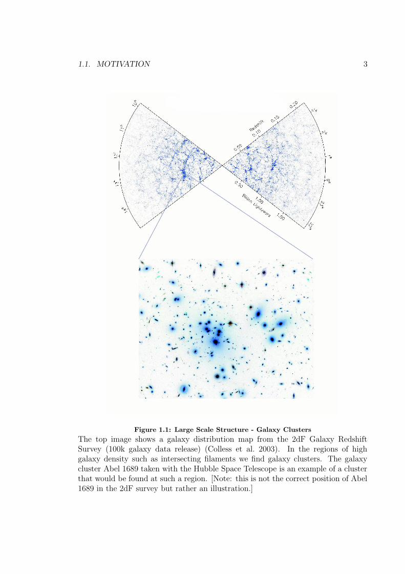
of such cosmic structures in the top panel of Figure 1.1 we see the distribution of
1
2 CHAPTER 1. INTRODUCTION
galaxies from the 2dF Galaxy Redshift Survey (Colless et al. 2001). This position-
ing of galaxies is clearly not random. Rather, the structure has a spongy/foamy
appearance. In this arrangement of galaxies there are regions with very few galaxies
(voids), and conversely there are filamentary structures consisting of many galax-
ies. At the intersection of these filaments we find the largest gravitationally bound
objects in the Universe; galaxy clusters, which are collections of hundreds or even
thousands of galaxies. One such galaxy cluster Abel 1689 can be seen in the bottom
of Figure 1.1.
The creation of structures in the Universe is a complicated process, requiring
many carefully measured ingredients, such as the right amount of matter and also
the type of matter is it baryonic or non-baryonic? Further, if a portion is non-
baryonic what is the nature of that matter? Does it interact? Is it hot, cold or
both? What is the geometry of the Universe? At what rate does the Universe
expand and does that expansion accelerate? How homogeneous and isotropic is the
Universe?
Recently through observation, significant progress has been made in answering
many of these questions and providing us with a compelling model for structure
formation. Arguably the most notable of these was the discovery of the cosmic
microwave background (CMB) (Penzias & Wilson 1965; de Bernardis et al. 2000;
Stompor et al. 2001; Spergel et al. 2003). The CMB is a remarkably uniform distri-
bution of microwave electromagnetic radiation looking back through the Universe
to when it was initially opaque. Imprinted on this uniform distribution are small
temperature fluctuations thought to have originated from inhomogeneities in the
distribution of matter on the surface of last scattering. From these temperature
variations we can place tight constrains on cosmological parameters including the
composition and density of the Universe. Further, it is these inhomogeneities that
are understood to have seeded structure formation The large galaxy redshift sur-
veys, such as the 2df galaxy redshift survey (Colless et al. 2001; Peacock et al. 2001)
and the Sloan Digital Sky Survey (York et al. 2000), have also been very significant,
placing complimentary constrain on the model through galaxy-clustering statistics.
The accuracy of these recent observations have allowed the establishment of the
so-called cosmological “concordance model”. This ΛCDM model consists of Cold
Dark Matter (CDM) in a flat, Lambda (Λ) dominated Universe comprised of 28%
dark matter, 68% dark energy, and luminous baryonic matter (i.e. galaxies, stars,
gas, and dust) at a mere 4% (cf. Spergel et al. 2003).
1.1. MOTIVATION 3
Figure 1.1: Large Scale Structure - Galaxy Clusters
The top image shows a galaxy distribution map from the 2dF Galaxy RedshiftSurvey (100k galaxy data release) (Colless et al. 2003). In the regions of highgalaxy density such as intersecting filaments we find galaxy clusters. The galaxycluster Abel 1689 taken with the Hubble Space Telescope is an example of a clusterthat would be found at such a region. [Note: this is not the correct position of Abel1689 in the 2dF survey but rather an illustration.]
4 CHAPTER 1. INTRODUCTION
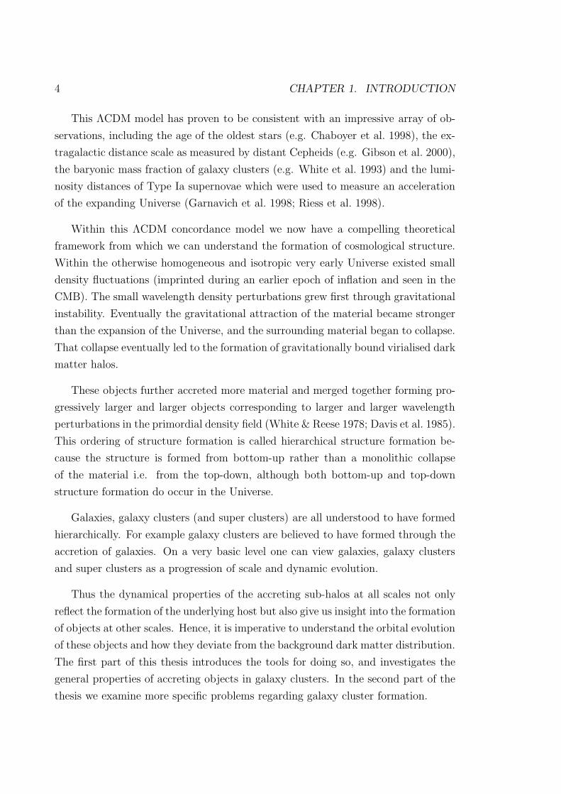
This ΛCDM model has proven to be consistent with an impressive array of ob-
servations, including the age of the oldest stars (e.g. Chaboyer et al. 1998), the ex-
tragalactic distance scale as measured by distant Cepheids (e.g. Gibson et al. 2000),
the baryonic mass fraction of galaxy clusters (e.g. White et al. 1993) and the lumi-
nosity distances of Type Ia supernovae which were used to measure an acceleration
of the expanding Universe (Garnavich et al. 1998; Riess et al. 1998).
Within this ΛCDM concordance model we now have a compelling theoretical
framework from which we can understand the formation of cosmological structure.
Within the otherwise homogeneous and isotropic very early Universe existed small
density fluctuations (imprinted during an earlier epoch of inflation and seen in the
CMB). The small wavelength density perturbations grew first through gravitational
instability. Eventually the gravitational attraction of the material became stronger
than the expansion of the Universe, and the surrounding material began to collapse.
That collapse eventually led to the formation of gravitationally bound virialised dark
matter halos.
These objects further accreted more material and merged together forming pro-
gressively larger and larger objects corresponding to larger and larger wavelength
perturbations in the primordial density field (White & Reese 1978; Davis et al. 1985).
This ordering of structure formation is called hierarchical structure formation be-
cause the structure is formed from bottom-up rather than a monolithic collapse
of the material i.e. from the top-down, although both bottom-up and top-down
structure formation do occur in the Universe.
Galaxies, galaxy clusters (and super clusters) are all understood to have formed
hierarchically. For example galaxy clusters are believed to have formed through the
accretion of galaxies. On a very basic level one can view galaxies, galaxy clusters
and super clusters as a progression of scale and dynamic evolution.
Thus the dynamical properties of the accreting sub-halos at all scales not only
reflect the formation of the underlying host but also give us insight into the formation
of objects at other scales. Hence, it is imperative to understand the orbital evolution
of these objects and how they deviate from the background dark matter distribution.
The first part of this thesis introduces the tools for doing so, and investigates the
general properties of accreting objects in galaxy clusters. In the second part of the
thesis we examine more specific problems regarding galaxy cluster formation.
1.1. MOTIVATION 5
Numerical Methods
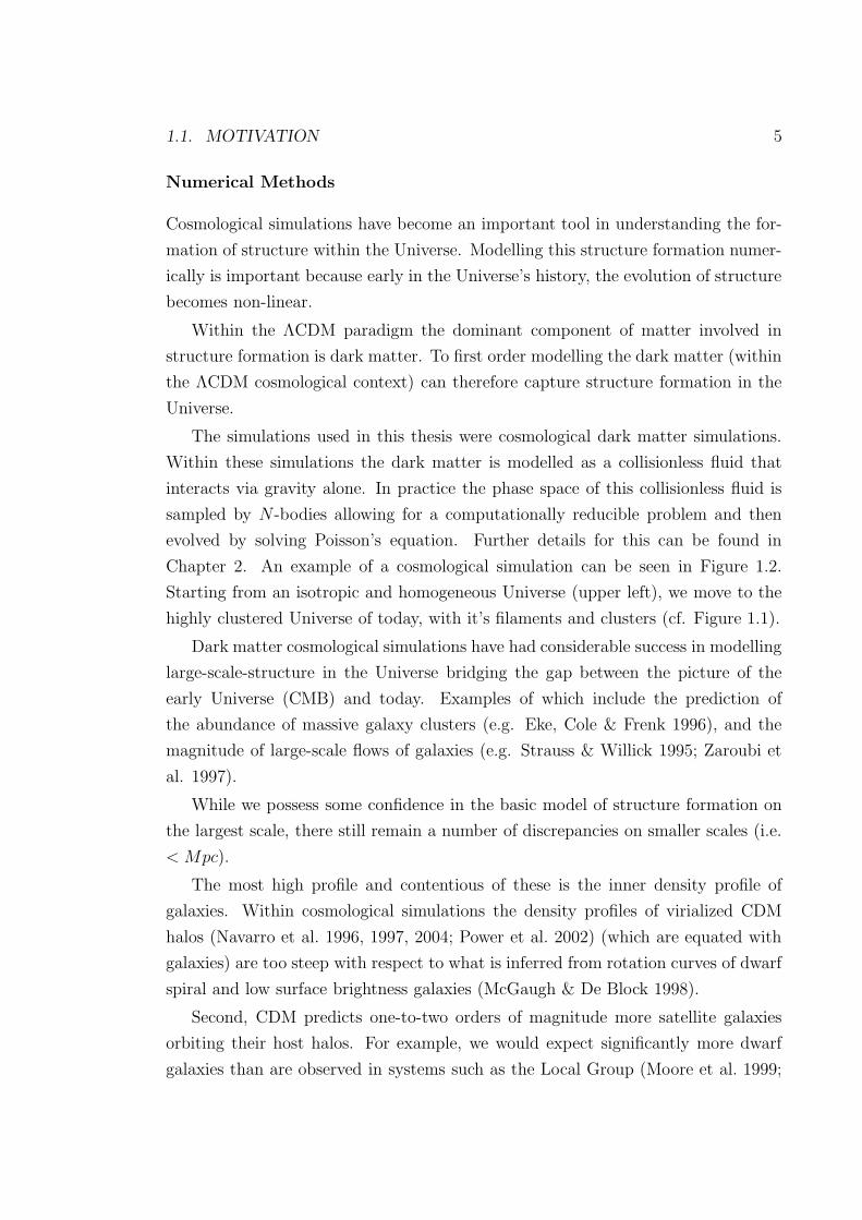
Cosmological simulations have become an important tool in understanding the for-
mation of structure within the Universe. Modelling this structure formation numer-
ically is important because early in the Universe’s history, the evolution of structure
becomes non-linear.
Within the ΛCDM paradigm the dominant component of matter involved in
structure formation is dark matter. To first order modelling the dark matter (within
the ΛCDM cosmological context) can therefore capture structure formation in the
Universe.
The simulations used in this thesis were cosmological dark matter simulations.
Within these simulations the dark matter is modelled as a collisionless fluid that
interacts via gravity alone. In practice the phase space of this collisionless fluid is
sampled by N -bodies allowing for a computationally reducible problem and then
evolved by solving Poisson’s equation. Further details for this can be found in
Chapter 2. An example of a cosmological simulation can be seen in Figure 1.2.
Starting from an isotropic and homogeneous Universe (upper left), we move to the
highly clustered Universe of today, with it’s filaments and clusters (cf. Figure 1.1).
Dark matter cosmological simulations have had considerable success in modelling
large-scale-structure in the Universe bridging the gap between the picture of the
early Universe (CMB) and today. Examples of which include the prediction of
the abundance of massive galaxy clusters (e.g. Eke, Cole & Frenk 1996), and the
magnitude of large-scale flows of galaxies (e.g. Strauss & Willick 1995; Zaroubi et
al. 1997).
While we possess some confidence in the basic model of structure formation on
the largest scale, there still remain a number of discrepancies on smaller scales (i.e.
< Mpc).
The most high profile and contentious of these is the inner density profile of
galaxies. Within cosmological simulations the density profiles of virialized CDM
halos (Navarro et al. 1996, 1997, 2004; Power et al. 2002) (which are equated with
galaxies) are too steep with respect to what is inferred from rotation curves of dwarf
spiral and low surface brightness galaxies (McGaugh & De Block 1998).
Second, CDM predicts one-to-two orders of magnitude more satellite galaxies
orbiting their host halos. For example, we would expect significantly more dwarf
galaxies than are observed in systems such as the Local Group (Moore et al. 1999;

6 CHAPTER 1. INTRODUCTION
Figure 1.2: Numerical Simulations of the Universe
In the top row, we see a numerical simulation of the formation of large scale structurein a ΛCDM Universe. The simulation begins on the upper left with an isotropic andhomogeneous Universe and evolves to the highly clustered Universe of today on theupper right with its filaments and clusters. The simulation box shows a region of100 Mpc. Zooming into a 2 Mpc region, we find a simulated galaxy cluster (bottomright). This simulated cluster is seen to resemble the observed cluster C10024+1654,whose map is constructed from an analysis of gravitational lensing (bottom left).Credit: Knebe A. and Kneib J.P
1.2. OUTLINE OF THE THESIS 7
Klypin et al. 1999a, Ghigna et al. 1998). A considerable amount of work has been
done to reconcile this discrepancy, with some suggesting suppressed star formation
is due to the removal of gas from the small protogalaxies by the ionising radiation
from the first stars and quasars (Bullock et al. 2000; Tully et al. 2002; Somerville
2002) thus leaving most of the satellites completely (or almost completely) dark.
Others suggest that the form of dark matter is incorrect appealing to Warm Dark
Matter (Knebe et al. 2002; Bode, Ostriker & Turok 2001; Colin et al. 2000).
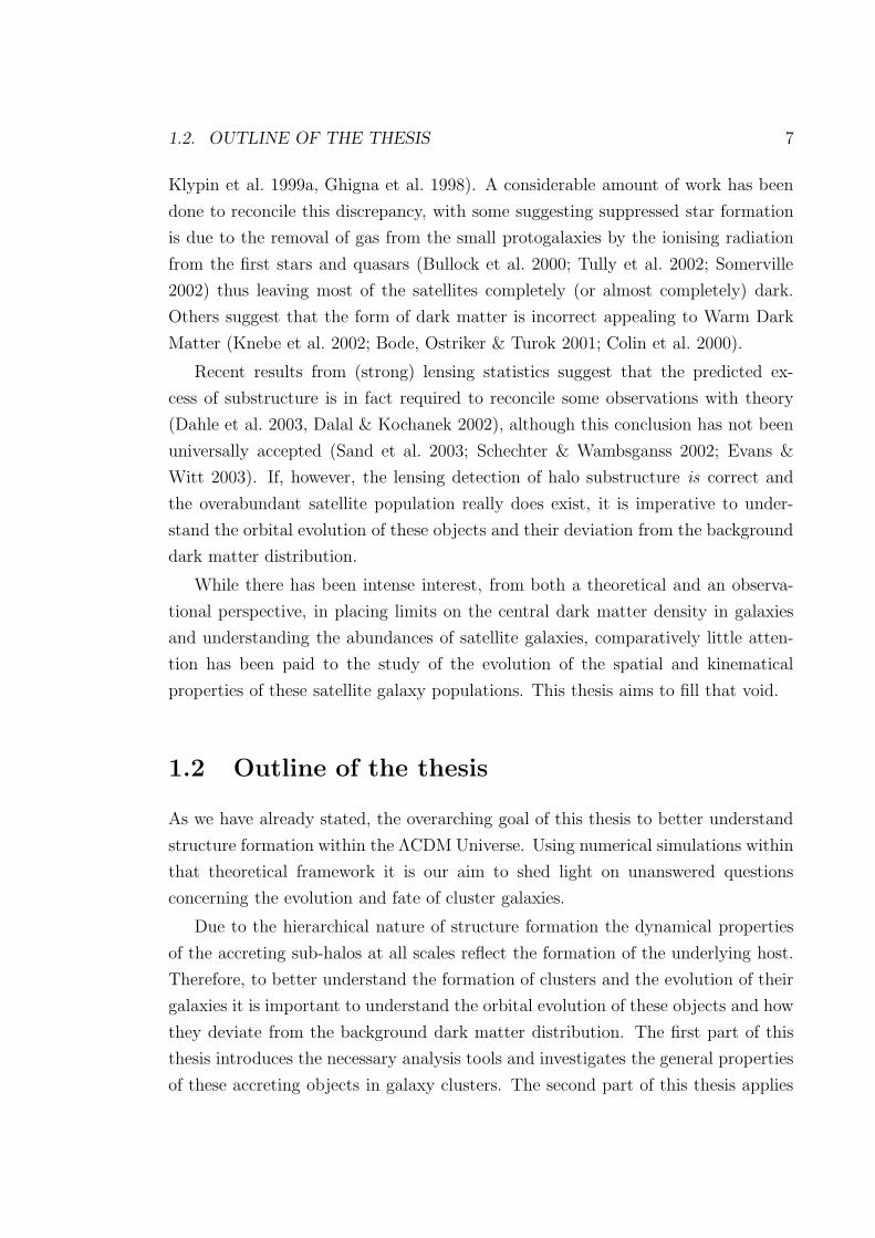
Recent results from (strong) lensing statistics suggest that the predicted ex-
cess of substructure is in fact required to reconcile some observations with theory
(Dahle et al. 2003, Dalal & Kochanek 2002), although this conclusion has not been
universally accepted (Sand et al. 2003; Schechter & Wambsganss 2002; Evans &
Witt 2003). If, however, the lensing detection of halo substructure is correct and
the overabundant satellite population really does exist, it is imperative to under-
stand the orbital evolution of these objects and their deviation from the background
dark matter distribution.
While there has been intense interest, from both a theoretical and an observa-
tional perspective, in placing limits on the central dark matter density in galaxies
and understanding the abundances of satellite galaxies, comparatively little atten-
tion has been paid to the study of the evolution of the spatial and kinematical
properties of these satellite galaxy populations. This thesis aims to fill that void.
1.2 Outline of the thesis
As we have already stated, the overarching goal of this thesis to better understand
structure formation within the ΛCDM Universe. Using numerical simulations within
that theoretical framework it is our aim to shed light on unanswered questions
concerning the evolution and fate of cluster galaxies.
Due to the hierarchical nature of structure formation the dynamical properties
of the accreting sub-halos at all scales reflect the formation of the underlying host.
Therefore, to better understand the formation of clusters and the evolution of their
galaxies it is important to understand the orbital evolution of these objects and how
they deviate from the background dark matter distribution. The first part of this
thesis introduces the necessary analysis tools and investigates the general properties
of these accreting objects in galaxy clusters. The second part of this thesis applies
8 CHAPTER 1. INTRODUCTION
these ideas and techniques to specific questions regarding the dynamics of galaxies
in clusters.
Each of the components of this thesis is based upon the series of N -body simu-
lations detailed in Chapter 2.
Part One
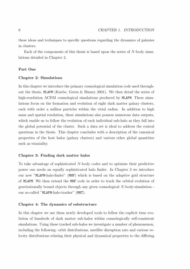
Chapter 2: Simulations
In this chapter we introduce the primary cosmological simulation code used through-
out the thesis, MLAPM (Knebe, Green & Binney 2001). We then detail the series of
high-resolution ΛCDM cosmological simulations produced by MLAPM. These simu-
lations focus on the formation and evolution of eight dark matter galaxy clusters,
each with order a million particles within the virial radius. In addition to high
mass and spatial resolution, these simulations also possess numerous data outputs,
which enable us to follow the evolution of each individual sub-halo as they fall into
the global potential of the cluster. Such a data set is ideal to address the central
questions in the thesis. This chapter concludes with a description of the canonical
properties of the host halos (galaxy clusters) and various other global quantities
such as triaxiality.
Chapter 3: Finding dark matter halos
To take advantage of sophisticated N -body codes and to optimise their predictive
power one needs an equally sophisticated halo finder. In Chapter 3 we introduce
our new ”MLAPM-halo-finder” (MHF) which is based on the adaptive grid structure
of MLAPM. We then extend the MHF code in order to track the orbital evolution of
gravitationally bound objects through any given cosmological N -body-simulation -
our so-called ”MLAPM-halo-tracker” (MHT).
Chapter 4: The dynamics of substructure
In this chapter we use these newly developed tools to follow the explicit time evo-
lution of hundreds of dark matter sub-halos within cosmologically self-consistent
simulations. Using these tracked sub-halos we investigate a number of phenomenon,
including the following: orbit distributions, satellite disruption rate and various ve-
locity distributions relating their physical and dynamical properties to the differing
1.2. OUTLINE OF THE THESIS 9
halo environmental conditions.
Part Two
Chapter 5: Anisotropy of substructure orbits
Nearby clusters such as Virgo and Coma possess galaxy distributions, which tend to
be aligned with the principal axis of the cluster itself. This has also been confirmed
by a recent statistical analysis of some 300 Abell clusters where the effect has been
linked to the dynamical state of the cluster (Plionis et al. 2002). In this chapter we
analyse our cluster simulations looking for this same alignment signal in the orbits
of the sub-halos.
Chapter 6: Outskirts of dark matter halos
It has been known for some time that galaxy properties in clusters are substantially
different from those of galaxies in the field (Hubble & Humason 1931; Oemler 1974;
Dressler 1980). However, the origins of these morphology-density relationships are
still not fully understood, with several large and small-scale mechanisms proposed
to explain their existence. To complement our earlier investigations on the dynamics
of sub-halos within the virial radii of the host halos, in this chapter we investigate
the galaxy populations in the outskirts of dark halos / galaxy clusters. In particular
we focus on the so-called “backsplash population”, i.e. satellite galaxies that once
were inside the virial radius of the host but now reside beyond it.
Chapter 7: Mapping substructure debris
Since the discovery of stellar streams in the Milky Way (Ibata et al. 2001c, Helmi
et al. 1999) and in M31 (Ibata et al. 2001a), and of streams and shells in clusters (
Trentham & Mobasher 1998), they have become standard fixtures in our understand-
ing of galaxy and cluster formation. These streams provide important observational
support for the hierarchical build-up of galaxies and clusters and the Λ-dominated
cold dark matter paradigm.
While previous studies focus on the disruption of satellite galaxies in static an-
alytical potentials, this chapter investigates their disruption in increasingly com-
plex potentials ultimately investigating the disruption of satellites within fully self-
consistent high-resolution cosmological galaxy clusters. For each of the simulations
10 CHAPTER 1. INTRODUCTION
we investigate the real and integrals-of-motion space distributions of the satellite
debris.
In the final chapter we outline the major conclusions of our research, and itemise
future work to be done.
Chapter 2
Simulations
“In the Universe there is a perfect form for everything,
and everything is a shadow of that perfect form.”
- Plato
2.1 Introduction
The N -body simulations used throughout this thesis were carried out using the
open source adaptive mesh refinement code MLAPM (Knebe, Green & Binney 2001).
In this Chapter we will present a brief introduction to MLAPM and explain why it
was an adequate choice of code for our studies. After introducing MLAPM we describe
how we simulated the eight dark matter galaxy clusters used throughout this thesis.
We conclude the chapter with a detailed look at these eight dark matter halos,
categorising their differences/similarities.
2.2 MLAPM
MLAPM (Multi-Level Adaptive Particle Mesh) is an open source C-code1for simulat-
ing the formation of structures from collisionless dark matter within a cosmological
framework. In the following section we will briefly review the fundamental compo-
nents of MLAPM.
1http://astronomy.swin.edu.au/MLAPM/
11

12 CHAPTER 2. SIMULATIONS
At the heart of MLAPM is the calculation of the gravitational forces. On the domain
grid (the cubic grid that covers the entire computational volume) MLAPM utilises
a multi-grid method based upon algorithms presented in Brandt (1977) & Press
et al. (1992) employing a finite-difference approximation to solve Possion’s equation.
Alternatively to this pure grid method for the solution of Possion’s equation on the
domain grid MLAPM also employs a Fast Fourier Transforms (FFT) method.
The limiting force resolution of the domain grid is conservatively estimated as
being twice the grid spacing. However, structure formation in the Universe occurs
over many orders of magnitude of scale, both in mass and space. To reach high mass
resolution MLAPM allows multiple mass species of particles; to reach high force reso-
lution, MLAPM refines its grids in high-density regions with an automated refinement
algorithm.
These adaptive meshes are recursive: refined regions can themselves be refined,
each subsequent refinement having cells that are half the size of the cells in the
parent level. This creates a hierarchy of refinement meshes of different resolutions
covering regions of interest. The refinement is done cell-by-cell (individual cells can
be refined or de-refined) and meshes are not constrained to have a rectangular (or
any other) shape. By having these nested grids we are able to increase the spatial
resolution of our simulation only where we require it, hence saving CPU time.
As with the multi-grid method for solving the potential on the domain grid,
the potential is solved on these arbitrarily shaped grids through a finite-difference
method. The difference between the refinement grids and the domain grids being
that instead of having a periodic boundary on the domain, the refinements are
solving an independent boundary problem, where the solution on the boundary is
fixed from the coarser parent grid.
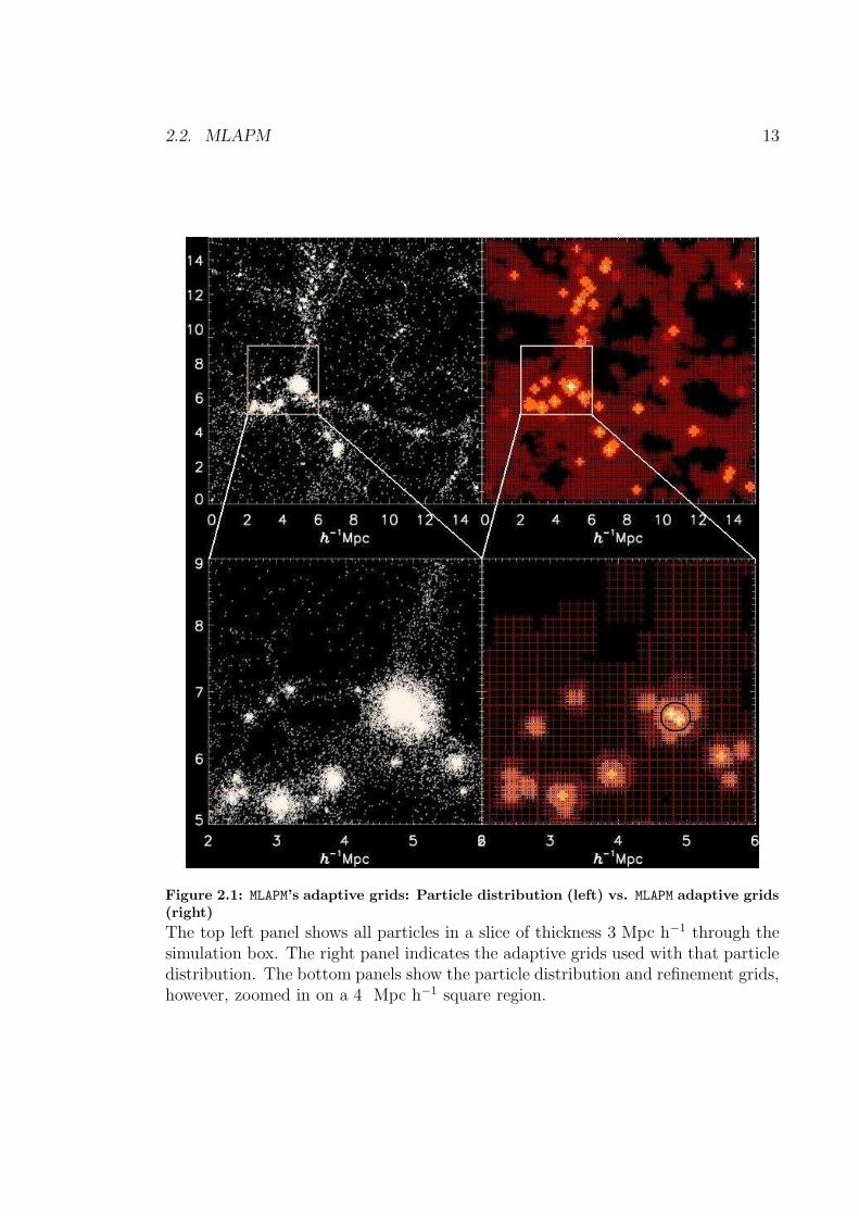
An example of MLAPM in action is shown in Figure 2.1. The top left panel shows
all particles in a slice of thickness 3 Mpc h−1 through the simulation box. The right
panel indicates the adaptive grids used with that particle distribution. The bottom
panels again show the particles’ distribution and refinement grids, however, zoomed
in on a 4 Mpc h−1 square region. In this region one can see the greater detail of the
refinement structures.
The criterion for (de-)refining a cell relates the number of particles within that
cell, the appropriate choice for this number having been described in detail by Knebe
et al. (2001). However, around each high density region a “buffer-zone” of refined
cells is created to ensure that the resolution of the grids changes gradually. In
2.2. MLAPM 13
Figure 2.1: MLAPM’s adaptive grids: Particle distribution (left) vs. MLAPM adaptive grids(right)
The top left panel shows all particles in a slice of thickness 3 Mpc h−1 through thesimulation box. The right panel indicates the adaptive grids used with that particledistribution. The bottom panels show the particle distribution and refinement grids,however, zoomed in on a 4 Mpc h−1 square region.
14 CHAPTER 2. SIMULATIONS
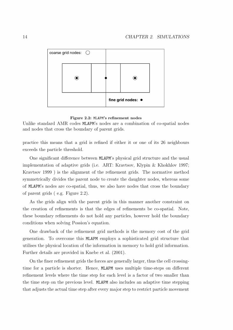
Figure 2.2: MLAPM’s refinement nodes
Unlike standard AMR codes MLAPM’s nodes are a combination of co-spatial nodesand nodes that cross the boundary of parent grids.
practice this means that a grid is refined if either it or one of its 26 neighbours
exceeds the particle threshold.
One significant difference between MLAPM’s physical grid structure and the usual
implementation of adaptive grids (i.e. ART: Kravtsov, Klypin & Khokhlov 1997;
Kravtsov 1999 ) is the alignment of the refinement grids. The normative method
symmetrically divides the parent node to create the daughter nodes, whereas some
of MLAPM’s nodes are co-spatial, thus, we also have nodes that cross the boundary
of parent grids ( e.g. Figure 2.2).
As the grids align with the parent grids in this manner another constraint on
the creation of refinements is that the edges of refinements be co-spatial. Note,
these boundary refinements do not hold any particles, however hold the boundary
conditions when solving Possion’s equation.
One drawback of the refinement grid methods is the memory cost of the grid
generation. To overcome this MLAPM employs a sophisticated grid structure that
utilises the physical location of the information in memory to hold grid information.
Further details are provided in Knebe et al. (2001).
On the finer refinement grids the forces are generally larger, thus the cell crossing-
time for a particle is shorter. Hence, MLAPM uses multiple time-steps on different
refinement levels where the time step for each level is a factor of two smaller than
the time step on the previous level. MLAPM also includes an adaptive time stepping
that adjusts the actual time step after every major step to restrict particle movement
2.3. SIMULATION SUITE 15
across a cell to a particular fraction of the cell spacing. This improves the accuracy
and reduces computational time.
2.3 Simulation Suite
Taking advantage of MLAPM’s ability to efficiently simulate structure in dense envi-
ronments through its adaptive grids, we have produced a series of high-resolution
cosmological simulations that have focused on the formation and evolution of eight
dark matter galaxy clusters, each containing of order a million particles.
To that end we first created a set of four independent initial conditions at red-
shift z = 45 in a standard ΛCDM cosmology (Ω0 = 0.3, Ωλ = 0.7, Ωbh2 = 0.04, h =
0.7, σ8 = 0.9). Next, 5123 particles were placed in a box of side length 64h−1 Mpc
giving a mass resolution of mp = 1.6 × 10⁸h−1 M. For each of these initial con-
ditions we iteratively collapsed the closest eight particles to one particle reducing
our particle number to 1283 particles. These lower mass resolution initial conditions
were then evolved until z = 0.
At z = 0, eight clusters from our simulation suite were selected in the mass
range 1–3×10¹⁴h−1 M, each sampling differing environmental conditions. Then, as
described by Katz (1994) and Ghigna (1998), for each cluster the particles within
three times the virial radius were tracked back to their initial positions of the start-
ing redshift (z = 45). Those particles were then regenerated to their original mass
resolution and positions, with the next layer of surrounding large particles regener-
ated only to one level (i.e. 8 times the original mass resolution), and the remaining
particles were left 64 times more massive than the particles resident with the host
cluster. This conservative criterion was selected in order to minimise contamination
of the final high-resolution halos with massive particles.
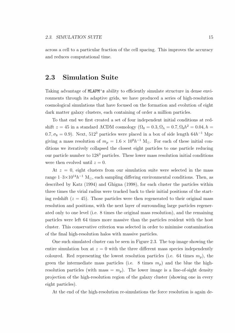
One such simulated cluster can be seen in Figure 2.3. The top image showing the
entire simulation box at z = 0 with the three different mass species independently
coloured. Red representing the lowest resolution particles (i.e. 64 times mp), the
green the intermediate mass particles (i.e. 8 times mp) and the blue the high-
resolution particles (with mass = mp). The lower image is a line-of-sight density
projection of the high-resolution region of the galaxy cluster (showing one in every
eight particles).
At the end of the high-resolution re-simulations the force resolution is again de-
16 CHAPTER 2. SIMULATIONS
Figure 2.3: Re-simulated Dark Matter halo
This figure shows the re-simulated Dark Matter halo (blue) and the parent simula-tion that hosted the re-simulated halo. The parent simulation (at z = 0) has boxsize 64h−1 Mpc and three different mass species. The red particles representing thelow-resolution simulation particles, the green particles the intermediate mass simu-lation particles and the blue particles the high-resolution simulation particles of there-simulated halo. In the bottom panel (for the re-simulated halo) the line-of-sightdensity is shown for one in every eight high-resolution particles.
2.4. HOST HALOS 17
termined by the highest refinement level reached. The whole computational volume
was covered by a regular domain grid consisting of 2563 cells. We had two separate
criteria for refinement, a domain cell was refined when there was more than one
particle per cell; further, every subsequent refinement was refined when there were
more than four particles per cell. Thus the finest grid at z = 0 consisted of 65,536
cells per side, giving a force resolution of ∼2h−1 kpc which allows us to resolve the
host halos down to the central ∼0.25% of the virial radii of the host halos (see
Table 2.5).
The halos chosen were selected to investigate the evolution of satellite galaxies
and their debris in an unbiased sample of host halos, exploring the influence of
environment upon the evolution of such systems.
To achieve this goal, excellent temporal resolution is required - as such we re-
tained 17 outputs from z = 2.5 to z = 0.5, equally spaced with ∆t ≈ 0.35Gyrs,
supplemented with an additional 30 outputs spanning z = 0.5 to z = 0 with
∆t ≈ 0.17Gyrs. As we show in the next chapter the average number of orbits
completed for our satellites is, one-to-two. Therefore we have 10-20 outputs avail-
able to accurately define the orbit of a given satellite, which is more than adequate
to trace a “live” orbit properly. We found that to sufficiently sample a live satellite
orbit one needs at least eight time-steps (Gill et al. 2004b).
2.4 Host halos
2.4.1 Canonical Properties
A simple analysis of the simulation at redshift z = 0 provides us with the relevant
information on the host halo. Defining the halo mass to be the total mass within
the virial radius Rvir, thus double counting the mass in the substructure and sub-
substructure, the halo masses ranged between 1–3 ×10¹⁴ h−1 M at z = 0. The
virial radii in turn were defined at the point where the mean averaged density of
the host (measured in terms of the cosmological background density ρb) drops below
∆vir = 340 with Mvir being the mass enclosed by that sphere. The formation redshift
zform is defined here as the redshift where the halo contained half of its present day
mass (Lacey & Cole 1994). Applying this criterion to our data we find that the ages
of our host halos range from 8.3 Gyrs to 3.4 Gyrs. In other words, while the masses
of our systems are comparable, they are of different dynamical age. In Table 2.5, as
18 CHAPTER 2. SIMULATIONS
in all following figures, the halos are ordered 1-8 in age.
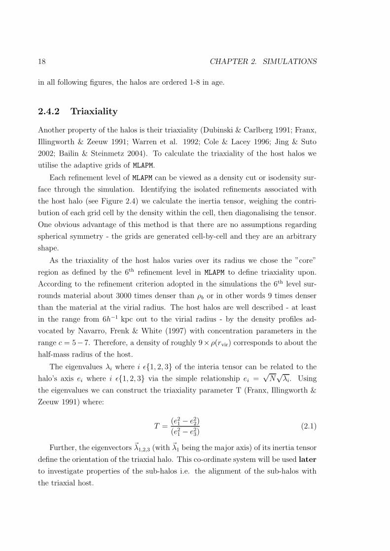
2.4.2 Triaxiality
Another property of the halos is their triaxiality (Dubinski & Carlberg 1991; Franx,
Illingworth & Zeeuw 1991; Warren et al. 1992; Cole & Lacey 1996; Jing & Suto
2002; Bailin & Steinmetz 2004). To calculate the triaxiality of the host halos we
utilise the adaptive grids of MLAPM.
Each refinement level of MLAPM can be viewed as a density cut or isodensity sur-
face through the simulation. Identifying the isolated refinements associated with
the host halo (see Figure 2.4) we calculate the inertia tensor, weighing the contri-
bution of each grid cell by the density within the cell, then diagonalising the tensor.
One obvious advantage of this method is that there are no assumptions regarding
spherical symmetry - the grids are generated cell-by-cell and they are an arbitrary
shape.
As the triaxiality of the host halos varies over its radius we chose the ”core”
region as defined by the 6th refinement level in MLAPM to define triaxiality upon.
According to the refinement criterion adopted in the simulations the 6th level sur-
rounds material about 3000 times denser than ρb or in other words 9 times denser
than the material at the virial radius. The host halos are well described - at least
in the range from 6h−1 kpc out to the virial radius - by the density profiles ad-
vocated by Navarro, Frenk & White (1997) with concentration parameters in the
range c = 5− 7. Therefore, a density of roughly 9× ρ(rvir) corresponds to about the
half-mass radius of the host.
The eigenvalues λi where i ε1, 2, 3 of the interia tensor can be related to the
halo’s axis ei where i ε1, 2, 3 via the simple relationship ei =√
N√
λi. Using
the eigenvalues we can construct the triaxiality parameter T (Franx, Illingworth &
Zeeuw 1991) where:
T =(e2
1 − e22)
(e21 − e2
3)(2.1)
Further, the eigenvectors ~λ1,2,3 (with ~λ1 being the major axis) of its inertia tensor
define the orientation of the triaxial halo. This co-ordinate system will be used later
to investigate properties of the sub-halos i.e. the alignment of the sub-halos with
the triaxial host.
2.4. HOST HALOS 19
Figure 2.4: Dark matter host halo triaxiality
This series of four images demonstrates the calculation of dark halo triaxiality. Thetop left image simply shows the line-of-sight projected density of a dark matterhalo (Halo #1), with the substructure removed. The bottom shows the same image,however, it also shows MLAPM refinement level # 6 in pink. The top right image showthe dark halo again, however, only showing 1 in every 32 particles, along with therefinement and the inferred ellipticity shown by the green ellipse. This green ellipseis easier to see in the bottom right image when we remove the MLAPM refinements.

20 CHAPTER 2. SIMULATIONS
2.4.3 Formation History
As we are interested in investigating the influence of host halo formation history and
environment on the orbital and internal properties of the satellites galaxies living
within its virial radius, it is important to understand how the host halos actually
formed.
As indicated by Tormen (1997) the formation of dark matter halos can be char-
acterised by two different phases: one corresponding to a rapid increase in halo
mass, representative of a major merger. We refer to this phase as a violent (V) pe-
riod. The second phase is one of relaxation in which the halo processes the merger
and settles toward virial equilibrium. A halo may continue to accrete smaller halos
during this phase. We refer to this phase as a quiet (Q) period.
The history of each halo is briefly outlined below using the simplified keys V or
Q to signify violent or quiet episodes. For example, halo #1 has a history “QVQQ”,
that is, a quiet period around the time of formation zform followed by a violent
period of merging of about the same length and completed by quiet evolution for
the remainder of the evolution, which lasts for twice as long as either of the two
earlier episodes. The coding chain splits the evolution since formation up into more-
or-less equal segments, but has nothing to say about the absolute timescales, which
differ widely from halo to halo. A qualitative summary of the eight halos follows:
Halo #1 (QVQQ)
A reasonably quiet history with no major violent encounters, save for a medium one
at z = 0.7.
Halo #2 (QVQQ)
A generally quiet history with a medium size merger one quarter of the way through
its evolution at z = 0.53, quickly settling for the rest of its formation.
Halo #3 (QVVVQ)
An initial short quiet period followed by a long and violent interaction that takes
essentially the rest of its formation time to settle.
Halo #4 (VQQ)
An initially violent merger which quickly settles for the rest of its formation.
Halo #5 (V)
A very violent formation history with a strongly oscillating potential.
Halo #6 (V)
A steady, yet violent, formation history.

2.5. SUMMARY AND CONCLUSION 21
Halo #7 (V)
A formation history quite similar to that of halo #6.
Halo #8 (V)
A rapid formation history; constantly interacting with two other large halos. In this
sense, a unique system.
While useful, such a qualitative description needs to be augmented with a quan-
titative one. In order to do so, we use the dispersion of the rate of relative mass
change of the host halos:
σ2∆M/M =
1
Nout
Nout∑
i=2
(
∆Mi
∆tiMi− 〈 ∆M
∆tM〉i
)2
, (2.2)
where Nout is the number of available outputs from formation zform to redshift z = 0,
∆Mi = M(zi) − M(zi−1) the change in the mass of the host halo, and ∆ti the
respective change in time. The mean growth rate at time i
〈 ∆M
∆tM〉i =
1
Ni
Ni∑
j=1
(
∆Mi
∆tiMi
)
j
(2.3)
is calculated for each individual output as the average over all halos Ni available at
that time step.
A large dispersion σ∆M/M indicates a violent formation history whereas low val-
ues correspond to quiescent formation histories. As we can see in Table 2.5, our
qualitative classification scheme is confirmed by the σ∆M/M values.
2.5 Summary and Conclusion
In this chapter we were briefly introduced to the cosmological simulation code MLAPM.
We then used that code to create a suite of eight simulated galaxy cluster dark matter
halos based on the re-simulation technique outlined by Katz (1994) and Ghigna
(1998). These cluster halos will become the base simulations used throughout the
thesis to investigate the populations of sub-halos (galaxies in our case) that exist
and are transformed within dark halos (clusters of galaxies for the simulations at
hand).
The final part of this chapter is dedicated to analysing and describing the dif-
ferences in the host halos. These host halos were chosen to sample a variety of

22 CHAPTER 2. SIMULATIONS
Table 2.1: Summary of the eight host dark matter halos. Distances are measured inh−1 Mpc, velocities in km s−1, masses in 1014
h−1 M, and the age in Gyrs.
Halo Rvir c V maxcirc Mvir zform age Triaxiality σ∆M/M form. hist.
# 1 1.34 8.7 1125 2.87 1.16 8.30 0.67 0.10 QVQQ# 2 1.06 9.6 894 1.42 0.96 7.55 0.87 0.10 QVQQ# 3 1.08 5.9 875 1.48 0.87 7.16 0.83 0.10 QVVVQ# 4 0.98 7.7 805 1.10 0.85 7.07 0.77 0.09 VQQ# 5 1.35 6.0 1119 2.91 0.65 6.01 0.65 0.15 V# 6 1.05 8.1 833 1.37 0.65 6.01 0.92 0.15 V# 7 1.01 6.6 800 1.21 0.43 4.52 0.89 0.25 V# 8 1.38 3.7 1041 3.08 0.30 3.42 0.90 0.22 V
triaxialities, formation times and mass/satellite accretion, despite being of compa-
rable mass. The halos also had very different formation histories, from quiescent to
violent. A summary of the eight host halos is presented in Table 2.5 where the halos
are presented and numbered from oldest to youngest.

Chapter 3
Finding Dark Matter Halos
“What I find most disheartening is the thought that
somewhere out there our galaxy has been deleted fromsomebody else’s sample.”
- Dr Alexander Boksenberg (1996)
3.1 Introduction
Over the last 30 years great progress has been made in the development of N -
body codes that model the distribution of dissipationless dark matter. Algorithms
have advanced considerably since the first N 2 particle-particle codes (Aarseth 1963;
Peebles 1970; Groth et al. 1977); we have seen the development of the tree-based
gravity solvers (Barnes & Hut 1986), mesh-based solvers (Klypin & Shandarin 1983),
then the two combined (Efstathiou et al. 1985) and multiple strands of adaptive and
deforming grid codes (Villumsen 1989; Suisalu & Saar 1995; Kravtsov, Klypin &
Khokhlov 1997; Bryan & Norman 1998; Knebe, Green & Binney 2001). While
they all push the limits of efficiency in computational resources, each code has
its individual advantages and limitations. The result of such research has been
highly reliable, cost effective codes. However, producing the data is only one step
in the process; the ensembles of millions of (dissipationless) dark matter particles
generated still require interpreting and then comparison to the real Universe. This
necessitates access to analysis tools to map the phase-space which is being sampled
by the particles onto “real” objects in the Universe; traditionally this has been
accomplished through the use of “halo finders”. Halo finders mine N -body data
23
24 CHAPTER 3. FINDING DARK MATTER HALOS
to find locally over-dense gravitationally bound systems, which are then attributed
to the dark halos we currently believe surround galaxies. Such tools have lead to
critical insights into our understanding of the origin and evolution of structure and
galaxies. To take advantage of sophisticated N -body codes and to optimise their
predictive power one needs an equally sophisticated halo finder.
Over the years, halo-finding algorithms have paralleled the development of their
partner N -body codes. We briefly outline the major halo finders currently in use:
The Friends-of-Friends (FOF) (Davis et al. 1985; Frenk et al. 1988) algorithm
uses spatial information to locate halos. Specifying a linking length blink the finder
links all pairs of particles with separation equal to or less than blink and calls these
pairs “friends”. Halos are defined by groups of friends (friends-of-friends) that have
at least one of these friendship connections. Two such advantages of this algorithm
are its ease of interpretation and its avoidance of assumption concerning the halo
shape. The greatest disadvantage is its simple choice of linking length which can lead
to a connection of two separate objects via so-called linking “bridges”. Moreover,
as structure formation is hierarchical, each halo contains substructure and thus the
need for different linking lengths to identify “halos-within-halos”. There have been
many variants to this scheme which attempt to overcome some of these limitations
(Suto, Cen & Ostriker 1992; Suginohara & Suto 1992; van Kampen 1995; Okamoto
& Habe 1999; Klypin et al. 1999b).
DENMAX (Bertschinger & Gleb 1991; Gleb & Bertschinger 1994) and SKID
(Weinberg, Hernquist & Katz 1997) are similar methods in that they both calculate
a density field from the particle distribution, then gradually move the particles in the
direction of the local density gradient ending with small groups of particles around
each local density maximum. The FOF method is then used to associate these small
groups with individual halos. A further check is employed to ensure that the grouped
particles are gravitationally bound. The two methods differ through their calculation
of the density field. DENMAX uses a grid while SKID applies an adaptive smoothing
kernel similar to that employed in Smoothed Particle Hydrodynamics techniques
(Lucy 1977; Gingold & Monaghan 1977; Monaghan 1992). The effectiveness of
these methods is limited by the method used to determine the density field (Gotz,
Huchra & Brandenberger 1998).
A similar technique to the above is the Bound Density Maxima (BDM) method
(Klypin & Holtzman 1997; Klypin et al. 1999b). In this scheme a smoothed density
is derived by smearing out the particle distribution on a scale rsmooth of order the
3.1. INTRODUCTION 25
force resolution of the N -body code used to generate the data. Randomly placed
“seed spheres” with radius rsmooth are then shifted to their local centre-of-mass in
an iterative procedure until convergence is reached. Hence, as with DENMAX and
SKID, this process finds local maxima in the density field. Bullock et al. (2001)
further refined the BDM technique by first generating a set of possible centres,
ranking the particles with respect to their local density and then implementing
modifications which allow for credible identification of halos-within-halos. The Bul-
lock et al. (2001) adaptation to BDM is geared towards finding halo substructure.
When one is primarily concerned with distinct halos, all the mentioned meth-
ods perform exceedingly well. All efforts to refine and enhance those halo finding
algorithms are due to the fact as we have seen in Chapter 1 that N -body codes
overcame overmerging only recently (Klypin et al. 1999b) and are capable of finding
satellites galaxies within dark matter host halos. It is therefore crucial to reliably
identify “halos-within-halos”. In fact, we saw that one of the remaining problems for
simulations of CDM structure formation is that high-resolution simulations nowa-
days predict far greater substructure (in total) than observed (Klypin et al. 1999a;
Moore et al. 1999).
Results from gravitational microlensing suggest that the majority of substructure
which does exist has to be close to the inner regions (Dalal & Kochanel 2002) which
thus far has not been confirmed by such simulations. There are recent claims that
although the (numerical) overmerging problem has disappeared in the outer regions
of the halo, the inner regions might still suffer from it (Taylor, Silk & Babul 2003).
As these latter semi-analytic models do not suffer from such numerical problems,
they find that such substructure does exist in the inner regions. The question though
arises as to whether there still remains an overmerging problem in the simulations or
if current halo finding algorithms actually do break down at those scales. As we will
discuss later, it becomes more difficult to locate peaks in the central region (if at all
present) of the host halo due to a simple lack of contrast to the dense background.
In this chapter we present a new method for identifying gravitationally bound
objects within cosmological simulations using the adaptive meshes of MLAPM. This
new code excels at finding “halos-within-halos” revealing more substructure in the
inner regions of the host halo. In its native form, our new algorithm works naturally
“on-the-fly”, but it has also been constructed with the flexibility necessary to handle
a single temporal output from any N -body code. Our analysis software is publicly

26 CHAPTER 3. FINDING DARK MATTER HALOS
available and packaged with both the MLAPM distribution1 and soon to be released
AMIGA code (the successor of MLAPM). The outline of the chapter is as follows. In
Section 3.2 we introduce the new halo finder “MLAPM-halo-finder” (MHF), describing
its functionality, advantages, and limitations. Section 3.3 provides a brief analysis
of the satellites found by MHF. In Section 3.4 we introduce the “MLAPM-halo-tracker”
(MHT) which augments the halo finder by incorporating the ability to track the
temporal evolution of satellites. Analysis of the halos tracked with MHT is described
in Section 3.5. We next compare the two methods with other publicly available
halo finding algorithms, such as FOF and SKID, in Section 3.6. In the second last
section, Section 3.7 we describe the additional changes to MHF. We conclude with a
summary and our conclusions in Section 3.8.
3.2 MHF: MLAPM’s Halo Finder
The general goal of a halo finder is to identify gravitationally bound objects. As all
halos are centred about local over-density peaks they are usually found simply by
using the spatial information provided by the particle distribution. Thus, the halos
are located as peaks in the density field of the simulation. To locate objects in this
fashion, the halo finder is required in some way to reproduce the work of the N -body
code in the calculation of the density field or the location of its peaks. When locating
halos like this, the major limitation will always be the appropriate reconstruction
of the density field. With that in mind we introduce MLAPM’s-Halo-Finder, MHF (or
simply Finder) hereafter.
MHF uses the adaptive grids of MLAPM to locate the satellites of the host halo.
As previously mentioned in Section 2, MLAPM’s adaptive refinement meshes follow
the density distribution by construction. Grid structure naturally “surrounds” the
satellites, as the satellites are simply manifestations of over-densities within (and
exterior) to the underlying host halo, a view which can best be appreciated through
inspection of Figure 3.1. In this figure, the refinement grids of MLAPM are superim-
posed over the projected density of the particle distribution. The top image is the
5th refinement level, with the 6th and 7th levels shown below. We emphasise that
the grids get successively smaller and are subsets of other grids on lower refinement
levels. The advantage of reconstructing and using these grids to locate halos is that
1http://www.aip.de/People/AKnebe/MLAPM/
3.2. MHF: MLAPM’S HALO FINDER 27
they naturally follow the density field with the exact accuracy of the N -body code.
No scaling length is required, in contrast with techniques such as FOF. Therefore,
MHF avoids one of the major complications inherent to most halo finding schemes as
a natural consequence of its construction.
To locate appropriate halos within our simulation outputs we first build a list of
“potential centres” for the halos. Using the full adaptive grid structure invoked by
MLAPM, with the same refinement criterion as for the original runs, we restructure the
hierarchy of nested isolated MLAPM grids into a “grid tree”. This reconstruction
is illustrated in Figure 3.2. Thus each of the branches of this tree is a Dark matter
halo, with the densest cell in the end of a branch marking a prospective Dark Matter
halo centre. This centre is then stored in a list of prospective halo centres.
Within a typical simulation (assuming a density cut at the virial density) one
can imagine a number of grid trees populating the simulation. Each one of these
trees would be a host halo with each branch being a sub-halo one of the branches is
the host!. However, because of the arbitrary way the grids are created each branch
can further, have branches thus we have sub-sub-halos. This embedded halo within
halo is obviously only limited by the simulation resolution.
Assuming that each of these peaks in MLAPM’s adaptive grids is the centre of a
halo, we step out in (logarithmically spaced) radial bins until the density reaches
ρsatellite(rvir) = ∆vir(z)ρb(z), where ρb is the universal background density, unless we
reach a point rtrunc where an upturn in the radial density profile is detected. This rise
is encountered for (almost) all satellites embedded within the background density
of the host halo, a point that we will discuss in more detail in Section 3.3. The
outer radius of the satellite is defined to be either rvir or rtrunc, whichever is smaller,
and dubbed rMHF. Using all particles interior to rMHF we calculate other canonical
properties for each halo such as its mass, rotation curve, and velocity dispersion.
We now, however, need to prune the list of (still prospective) halos. The first step
in this process is to check if there are any duplicate halos (One could imagine that
we caught two halos in the very final stages of merging.) Thus for each satellite a set
of “duplicate candidates” is constructed based on the criterion that their centres lie
within each others’ outer radii rMHF. Then, this list is then evaluated by comparing
the internal properties of the candidates. A candidate was affirmed to be a duplicate
once its mass, velocity dispersion, and centre of mass velocity vector agreed to within
80%. We then kept the halo with the higher central density and removed the other
one from the satellite catalogue completely. This is a rare circumstance, yet one to

28 CHAPTER 3. FINDING DARK MATTER HALOS
Figure 3.1: MLAPM’s refinement grid structure
This panel shows a series of 3 consecutive refinement levels of MLAPM’s grid structurestarting at the 5th refinement level superimposed upon the density projection of theparticle distribution.

3.2. MHF: MLAPM’S HALO FINDER 29
Figure 3.2: MHF’s “grid tree” reconstruction
This figure illustrates the restructuring of the nested MLAPM grids into to the “gridtree”. The left side represents an idealised refinement grid structure, while the rightside shows the re-ordering of these grids into a “grid tree”. Note that each branchof the grid tree represents a single dark matter halo within the simulation.
which we will return in Section 3.3.
With our nearly complete set of halos now in hand, we proceed to remove grav-
itationally unbound particles. This again is done in an iterative process. Starting
with the MHF halo centre, we calculate the kinetic and potential energy for each
individual particle in the respective reference frame and all particles faster than
two times the escape velocity are removed from the halo. We then recalculate the
centre, and proceed through the process again. This pruning is halted when a given
halo holds fewer than the stated minimum number of particles or when no further
particles need to be removed. This procedure also accounts for the rare instances
that isolated grids were generated through numerical noise or coincidence (i.e. the
crossing of two debris streams) since these halos are very small and contain unbound
members.
We finish by recalculating the internal properties of the halos with the radial
density profiles of the satellites fitted to the functional form proposed by Navarro,
Frenk & White (1997). Note we use the cumulative rather than the differential
density profile to increase our number statistics.
ρcum(r) =M(<r)
4π3
r3∝ 1
(r/rs)(1 + r/rs)2. (3.1)
30 CHAPTER 3. FINDING DARK MATTER HALOS
in the range from 8h−1 kpc (≈ 4×force resolution) to rMHF. The scale radius rs is
used to define the concentration of the halo
c = rvir/rs. (3.2)
The procedure outlined above naturally deals with overlapping halos and sub-
structure halos, respectively. But as mentioned before, for such objects the virial
radius can not be determined properly as we will observe a rise in the radially binned
density profile due to the overlap with another halo or the embedding into the host.
In that case we set the outer radius of the (sub-)halo to be that point where the
density profile rises and all canonical properties are derived using all (gravitationally
bound!) particles interior to that radius. And the fit to an NFW profile Eq. (3.1) is
only done out to that radius, too. The situation is different once both of the over-
lapping halo’s centres are within each other’s virial/upturn radius: we then checked,
if those two objects are just duplicates by comparing their internal properties.
As stated in 2, it is our aim to investigate the evolution of satellite galaxies within
their host halos. Thus, we restrict our satellites to having at least 50 high-resolution
simulation particles, which corresponds to a mass-cut of Mcut ≈ 1010h−1 M. More-
over, each satellite must contain at least 50% percent of its mass in high-resolution
particles. In practice, this latter constraint is not a critical one, relevant only for
satellites well beyond twice the host halo’s virial radius.
MHF is implemented into MLAPM in a way that provides the user simultaneously
with a snapshot of the dark matter particles and halo catalogues at each required
output. The most obvious advantages of having the analysis performed “on the fly”
are the reduction in computer and human hours in the initial halo analysis stage.
Embedding the halo analysis in the code also enables us to potentially analyse the
data at unprecedented time resolution, if required.2 However, MHF can also be used
with any already existing single time-step snapshot and hence is not limited to
data produced by MLAPM; it can also be used for any N -body output provided the
latter is converted to MLAPM’s binary format using the tools included in the MLAPM
distribution. However, to this date read routines for TIPSY and GADGET (version
1) and GADGET-2 formats are implemented within MLAPM and hence MHF.
2MHF can be switched on either to act only when writing an output file (-DMHF) or at eachindividual time step (-DMHFstep).

3.3. ANALYSIS OF MHF HALOS 31
3.3 Analysis of MHF halos
MHF was applied to each of the 376 temporal outputs (47 outputs per each of the
eight independent halos), providing us with a list of all satellites and their internal
properties at each individual redshift under consideration. As stated earlier, the
detailed analysis of the science associated with these satellites presented in proceed-
ing chapters. We do however wish to highlight several key preliminary results here
which relate specifically to the halo identification process.
In Figure 3.3 we plot the normalised number of satellites as a function of nor-
malised radius. One, perhaps not surprising, aspect of Figure 3.3 is the similarity
in the slopes. Although the number of satellites in each halo may vary, the relative
radial distribution of the satellites is similar across halos. This is reminiscent of
the universal density profile of dark matter halos, as described by Navarro, Frenk &
White (1997). Although the radial distribution of the satellites remains consistent,
there exists a range of substructure densities for the halos, as there is a spread in
the number of satellites within each halo (recall Table 1). Therefore, we should be
able to distinguish the effects of substructure density on the physical properties of
the satellites.
The other striking feature of Figure 3.3 is the lack of satellites in the inner 15%
of the virial radius. One might ask why this is the case. Does it indicate that
satellites dynamically avoid the central region of the halo? Perhaps they simply
do not spend much time there? Perhaps via physical means satellites that ven-
ture near the centre are either merged or experience such strong tidal forces that
they are destroyed? Perhaps we are simply dominated by numerical effects and are
witnessing the premature destruction of halos in dense environments. This latter
problem - known as overmerging - affected low-resolution dissipationless simulations
in the early 1990s, failing to produce galaxy-sized dark matter halos in clusters (e.g.
Summers et al. 1995; van Kampen 1995; Moore et al. 1996). Traditionally, this
was explained by the lack of dissipation in the simulations. With the inclusion
of a baryonic component, denser objects could form and survive in the centres of
these dense regions. However, with the onset of higher resolution simulations a con-
verse effect was encountered - specifically, an abundance of substructure was found
(Klypin et al. 1999b).
The explanation of overmerging (or substructure disruption) was accredited to
numerical limitations in the simulations. van Kampen (1995) found that parti-

32 CHAPTER 3. FINDING DARK MATTER HALOS
Figure 3.3: Radial distribution of satellites: MHF
Number of satellites (normalised) orbiting within the virial radius of the host haloat z = 0, as a function of radial distance r, normalised by the virial radius of therespective host Rvir.
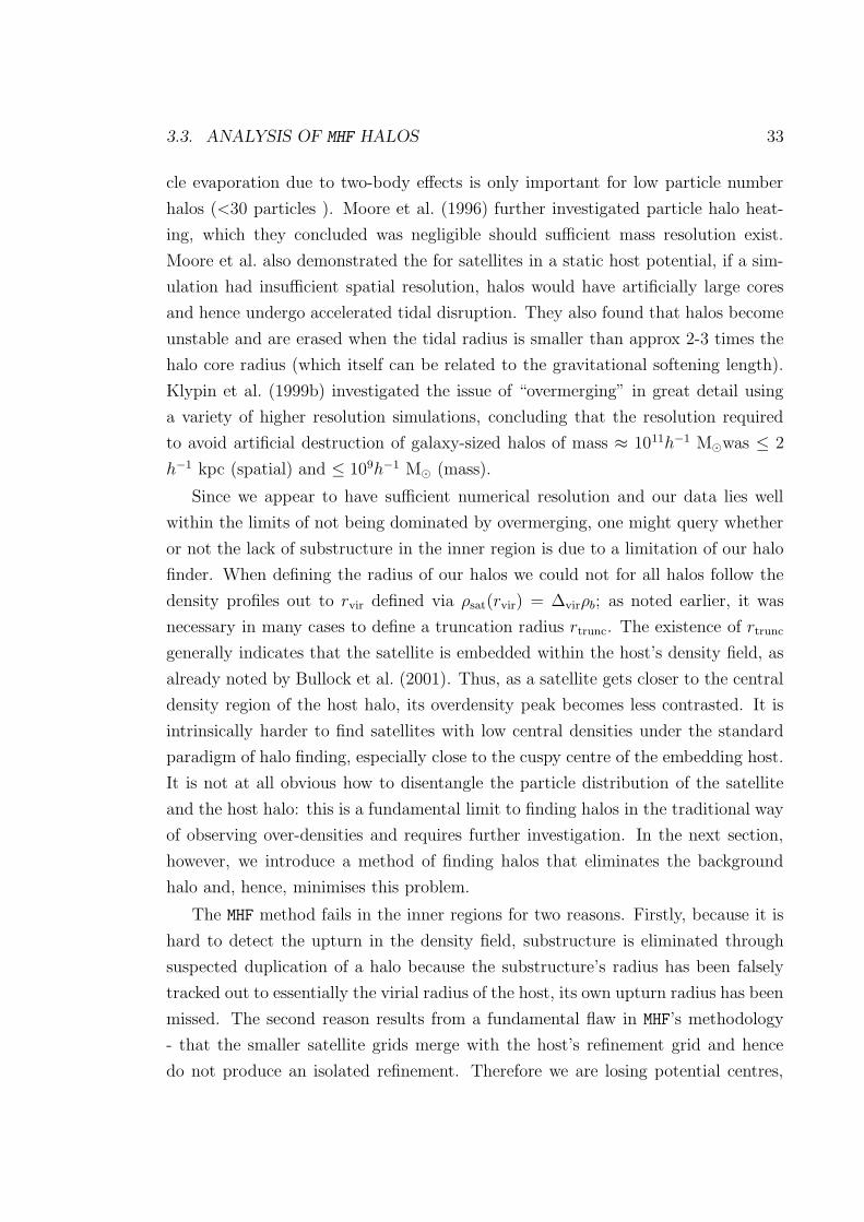
3.3. ANALYSIS OF MHF HALOS 33
cle evaporation due to two-body effects is only important for low particle number
halos (<30 particles ). Moore et al. (1996) further investigated particle halo heat-
ing, which they concluded was negligible should sufficient mass resolution exist.
Moore et al. also demonstrated the for satellites in a static host potential, if a sim-
ulation had insufficient spatial resolution, halos would have artificially large cores
and hence undergo accelerated tidal disruption. They also found that halos become
unstable and are erased when the tidal radius is smaller than approx 2-3 times the
halo core radius (which itself can be related to the gravitational softening length).
Klypin et al. (1999b) investigated the issue of “overmerging” in great detail using
a variety of higher resolution simulations, concluding that the resolution required
to avoid artificial destruction of galaxy-sized halos of mass ≈ 1011h−1 Mwas ≤ 2
h−1 kpc (spatial) and ≤ 109h−1 M (mass).
Since we appear to have sufficient numerical resolution and our data lies well
within the limits of not being dominated by overmerging, one might query whether
or not the lack of substructure in the inner region is due to a limitation of our halo
finder. When defining the radius of our halos we could not for all halos follow the
density profiles out to rvir defined via ρsat(rvir) = ∆virρb; as noted earlier, it was
necessary in many cases to define a truncation radius rtrunc. The existence of rtrunc
generally indicates that the satellite is embedded within the host’s density field, as
already noted by Bullock et al. (2001). Thus, as a satellite gets closer to the central
density region of the host halo, its overdensity peak becomes less contrasted. It is
intrinsically harder to find satellites with low central densities under the standard
paradigm of halo finding, especially close to the cuspy centre of the embedding host.
It is not at all obvious how to disentangle the particle distribution of the satellite
and the host halo: this is a fundamental limit to finding halos in the traditional way
of observing over-densities and requires further investigation. In the next section,
however, we introduce a method of finding halos that eliminates the background
halo and, hence, minimises this problem.
The MHF method fails in the inner regions for two reasons. Firstly, because it is
hard to detect the upturn in the density field, substructure is eliminated through
suspected duplication of a halo because the substructure’s radius has been falsely
tracked out to essentially the virial radius of the host, its own upturn radius has been
missed. The second reason results from a fundamental flaw in MHF’s methodology
- that the smaller satellite grids merge with the host’s refinement grid and hence
do not produce an isolated refinement. Therefore we are losing potential centres,
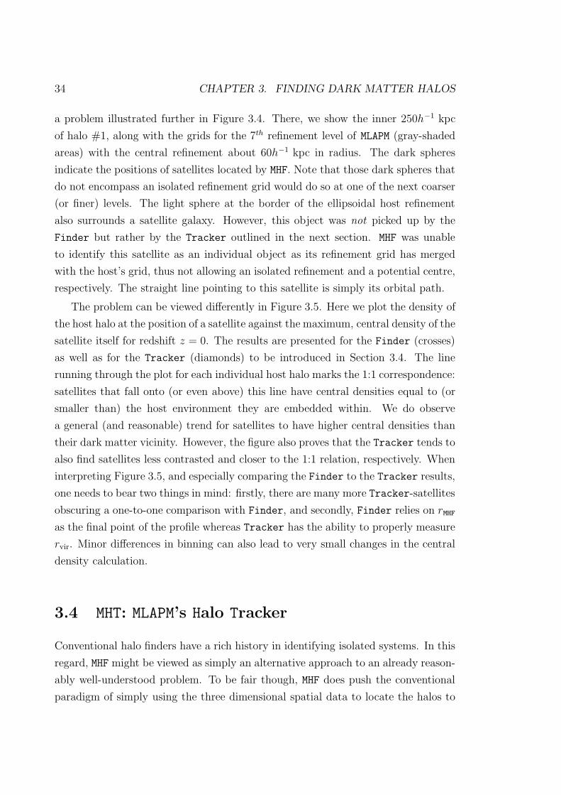
34 CHAPTER 3. FINDING DARK MATTER HALOS
a problem illustrated further in Figure 3.4. There, we show the inner 250h−1 kpc
of halo #1, along with the grids for the 7th refinement level of MLAPM (gray-shaded
areas) with the central refinement about 60h−1 kpc in radius. The dark spheres
indicate the positions of satellites located by MHF. Note that those dark spheres that
do not encompass an isolated refinement grid would do so at one of the next coarser
(or finer) levels. The light sphere at the border of the ellipsoidal host refinement
also surrounds a satellite galaxy. However, this object was not picked up by the
Finder but rather by the Tracker outlined in the next section. MHF was unable
to identify this satellite as an individual object as its refinement grid has merged
with the host’s grid, thus not allowing an isolated refinement and a potential centre,
respectively. The straight line pointing to this satellite is simply its orbital path.
The problem can be viewed differently in Figure 3.5. Here we plot the density of
the host halo at the position of a satellite against the maximum, central density of the
satellite itself for redshift z = 0. The results are presented for the Finder (crosses)
as well as for the Tracker (diamonds) to be introduced in Section 3.4. The line
running through the plot for each individual host halo marks the 1:1 correspondence:
satellites that fall onto (or even above) this line have central densities equal to (or
smaller than) the host environment they are embedded within. We do observe
a general (and reasonable) trend for satellites to have higher central densities than
their dark matter vicinity. However, the figure also proves that the Tracker tends to
also find satellites less contrasted and closer to the 1:1 relation, respectively. When
interpreting Figure 3.5, and especially comparing the Finder to the Tracker results,
one needs to bear two things in mind: firstly, there are many more Tracker-satellites
obscuring a one-to-one comparison with Finder, and secondly, Finder relies on rMHF
as the final point of the profile whereas Tracker has the ability to properly measure
rvir. Minor differences in binning can also lead to very small changes in the central
density calculation.
3.4 MHT: MLAPM’s Halo Tracker
Conventional halo finders have a rich history in identifying isolated systems. In this
regard, MHF might be viewed as simply an alternative approach to an already reason-
ably well-understood problem. To be fair though, MHF does push the conventional
paradigm of simply using the three dimensional spatial data to locate the halos to

3.4. MHT: MLAPM’S HALO TRACKER 35
Figure 3.4: Limitaions of the MHF paradigm
The inner 250 h−1 kpc of halo #1 with the particles’ line of sight density shown.We show the grids of the 7th refinement level of MLAPM, with the central refinementabout 60h−1 kpc in radius. The dark spheres represent the satellites located by MHF.The light sphere surrounds a satellite galaxy not found by MHF. The apparent sizes ofthe spheres are simply a visualisation effect as spheres farther away from the virtualobserver appear smaller.
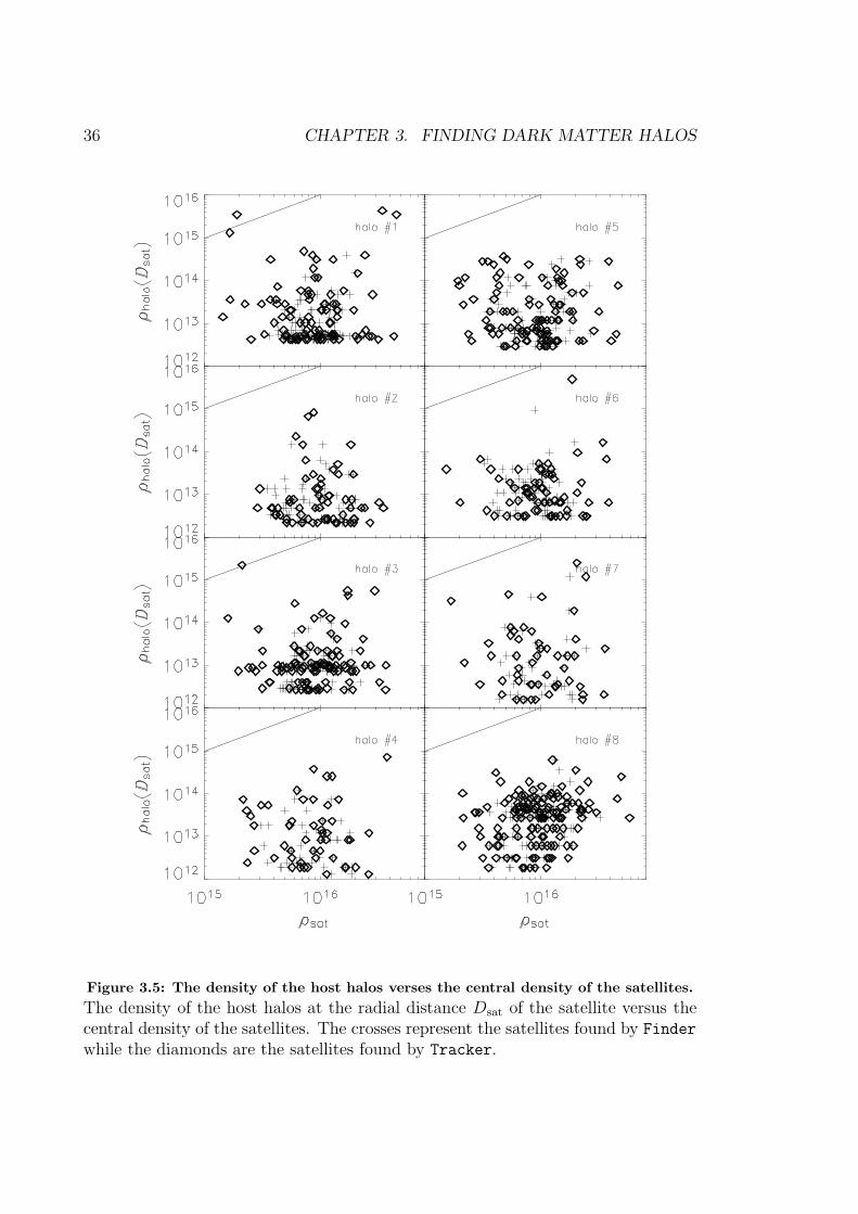
36 CHAPTER 3. FINDING DARK MATTER HALOS
Figure 3.5: The density of the host halos verses the central density of the satellites.
The density of the host halos at the radial distance Dsat of the satellite versus thecentral density of the satellites. The crosses represent the satellites found by Finder
while the diamonds are the satellites found by Tracker.

3.4. MHT: MLAPM’S HALO TRACKER 37
the limit, locating the halos with (nearly) the exact accuracy of the N -body code.
Having this ability, MHF becomes the ideal halo finder to locate substructure for
MLAPM and no doubt an excellent halo finder for other codes. Although, as we have
seen in Section 3.3, apart from numerical limitations in N -body codes (e.g. over-
merging) there still remain limitations to our current halo finders. These limitations
become a problem in the simulations when considering the substructure of any dense
system, for example galaxy clusters and galaxies. Therefore, to successfully find the
substructure we need to change the paradigm used to find it.
To successfully make this change we must first understand the environment in
which we are finding the substructure and then exploit its characteristics. One
characteristic is that most halos conserve their identities, that is substructure halos
rarely undergo mergers in halos because of their high relative velocities (Ghigna
et al. 1998; Okamoto & Habe 1999). Further, halos in dense environments undergo
tidal stripping and substructure interactions, no longer accreting material, but being
stripped of it. Thus in such environments it is sufficient to trace the particles of
the satellite once the satellite has entered the host’s virial radius. In this section we
introduce MLAPM’s-Halo-Tracer, MHT (or simply Tracker) hereafter.
MHT takes an arbitrary output of our new MLAPM-based halo finder MHF, and
correlates the particles for an arbitrary number of time steps using all simulation
outputs from that initial output until redshift z = 0. In our particular investigation
it was appropriate to define that initial arbitrary output to be the formation time
zform of the host halo or the time when the host halo contained half of its present
mass (Lacey & Cole 1994). We then followed all the satellites that were within two
times the virial radius of the host halo at this formation time. Although, we miss
a few satellites due to MHF’s identification limitations in the inner 10-15% of the
halo, from this time on MHT precisely follows the orbits of our initial set of satellites
irrespective how close they come to the host’s centre. An example of MHT in action
can be seen in Figure 3.6 and in Figure 3.7.
In Figure 3.6 we see a tracked satellite galaxy (dark matter substructure). The
line represents the satellite’s orbit going from yellow (past) to magenta (now). From
this figure we can see that the satellite initially fell into the host halo and has since
undergone two full orbits and is coming back for a third. When we started tracking
the satellite it was a gravitationally bound collection of particles, however, during
its orbit the satellite has undergone significant tidal stripping, as is indicated by
the stream of red particles. One interesting aside is that unlike the disruption of

38 CHAPTER 3. FINDING DARK MATTER HALOS
Figure 3.6: An example of a tracked satellite
a tracked satellite galaxy (dark matter substructure). The line represents the satel-lite’s orbit going from yellow (past) to magenta (now). From this figure we cansee that the satellite initially fell into the host halo and has since undergone twofull orbits and is coming back for a third. When we started tracking the satelliteit was a gravitationally bound collection of particles, however, during its orbit thesatellite has undergone significant tidal stripping, as is indicated by the stream ofred particles.
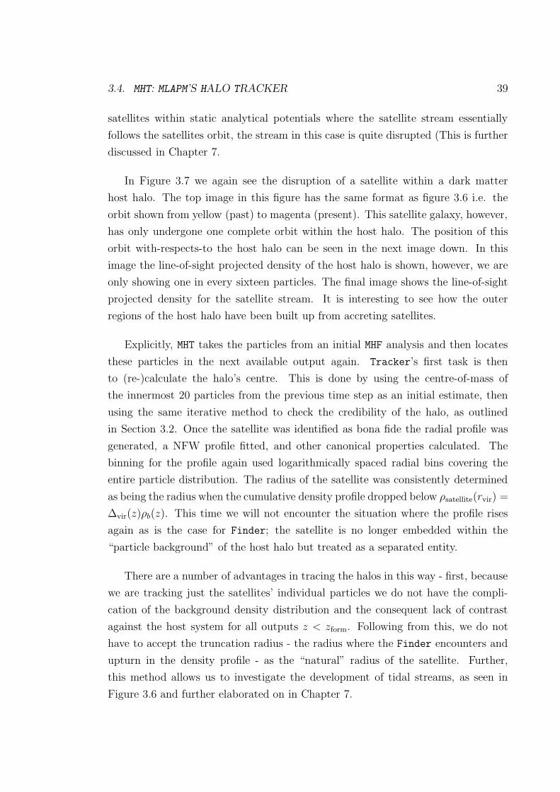
3.4. MHT: MLAPM’S HALO TRACKER 39
satellites within static analytical potentials where the satellite stream essentially
follows the satellites orbit, the stream in this case is quite disrupted (This is further
discussed in Chapter 7.
In Figure 3.7 we again see the disruption of a satellite within a dark matter
host halo. The top image in this figure has the same format as figure 3.6 i.e. the
orbit shown from yellow (past) to magenta (present). This satellite galaxy, however,
has only undergone one complete orbit within the host halo. The position of this
orbit with-respects-to the host halo can be seen in the next image down. In this
image the line-of-sight projected density of the host halo is shown, however, we are
only showing one in every sixteen particles. The final image shows the line-of-sight
projected density for the satellite stream. It is interesting to see how the outer
regions of the host halo have been built up from accreting satellites.
Explicitly, MHT takes the particles from an initial MHF analysis and then locates
these particles in the next available output again. Tracker’s first task is then
to (re-)calculate the halo’s centre. This is done by using the centre-of-mass of
the innermost 20 particles from the previous time step as an initial estimate, then
using the same iterative method to check the credibility of the halo, as outlined
in Section 3.2. Once the satellite was identified as bona fide the radial profile was
generated, a NFW profile fitted, and other canonical properties calculated. The
binning for the profile again used logarithmically spaced radial bins covering the
entire particle distribution. The radius of the satellite was consistently determined
as being the radius when the cumulative density profile dropped below ρsatellite(rvir) =
∆vir(z)ρb(z). This time we will not encounter the situation where the profile rises
again as is the case for Finder; the satellite is no longer embedded within the
“particle background” of the host halo but treated as a separated entity.
There are a number of advantages in tracing the halos in this way - first, because
we are tracking just the satellites’ individual particles we do not have the compli-
cation of the background density distribution and the consequent lack of contrast
against the host system for all outputs z < zform. Following from this, we do not
have to accept the truncation radius - the radius where the Finder encounters and
upturn in the density profile - as the “natural” radius of the satellite. Further,
this method allows us to investigate the development of tidal streams, as seen in
Figure 3.6 and further elaborated on in Chapter 7.
40 CHAPTER 3. FINDING DARK MATTER HALOS
Figure 3.7: A series of images showing a disrupted satellite and its relation to thehost halo.
In the top image we se that satellite galaxy, has undergone one complete orbit withinthe host halo. The position of this orbit with-respects-to the host halo can be seen inthe middle image. In this image the line-of-sight projected density of the host halois shown (showing 1 in every 16 particles). The final image shows the line-of-sightprojected density for the satellite stream.
3.5. ANALYSIS OF MHT HALOS 41
3.5 Analysis of MHT halos
The nature of hierarchical structure formation, i.e. mergers, dynamical and tidal
destruction of substructure, requires us to work harder when applying MHT to our
simulation data. Even though were are now tracing the initially bound particles
forward in time, we need a criterion to decide whether a satellite galaxy is disrupted
or still alive. We therefore introduce the tidal radius as given below.
3.5.1 Tidal Radius
The tidal radius is defined to be the radius of the satellite where the gravitational
effects of the host halo are greater than the self-gravity of the satellite. When
approximating the host halo and the satellite as point masses and maintaining that
the mean density within the satellite has to be three times the mean density of
the host halo within the satellites distance D to the host halo (Jacobi limit) the
definition for tidal radius reads as follows
rtidal =( m
3M
)13D , (3.3)
where m is the mass of the satellite and M = M(< D) is the mass of the host halo
internal to the distance D.
In order to stabilise the determination of the tidal radius rtidal we actually use
an iterative procedure again. By defining the satellite mass m as the mass internal
to rtidal, i.e. m = m(< rtidal), we find rtidal by solving
rtidal −(
m(< rtidal)
3M
)3
D = 0 . (3.4)
Starting with the distance of the furthest particle in the satellite particle distribution
as the initial guess for rtidal, the method quickly converges in two-to-three iterations.
3.5.2 Satellite Disruption
As the satellites orbit within the host halo they undergo tidal stripping, hence, the
satellites are gradually losing mass. Therefore, their particle distribution becomes
more and more diffuse, reducing the tidal radius of the satellite. Eventually there
comes a point when the satellite loses sufficient mass that we begin to reach the
limits of our numerical resolution, not having sufficient number of particles to follow
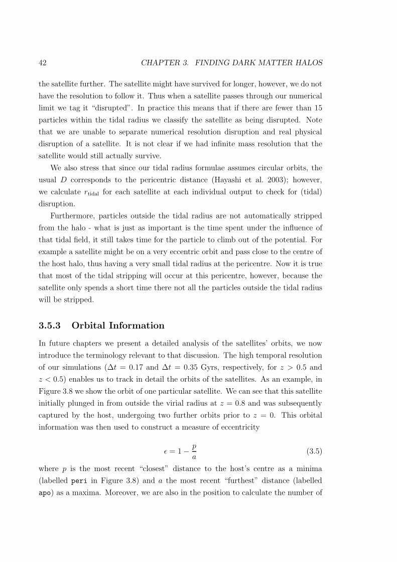
42 CHAPTER 3. FINDING DARK MATTER HALOS
the satellite further. The satellite might have survived for longer, however, we do not
have the resolution to follow it. Thus when a satellite passes through our numerical
limit we tag it “disrupted”. In practice this means that if there are fewer than 15
particles within the tidal radius we classify the satellite as being disrupted. Note
that we are unable to separate numerical resolution disruption and real physical
disruption of a satellite. It is not clear if we had infinite mass resolution that the
satellite would still actually survive.
We also stress that since our tidal radius formulae assumes circular orbits, the
usual D corresponds to the pericentric distance (Hayashi et al. 2003); however,
we calculate rtidal for each satellite at each individual output to check for (tidal)
disruption.
Furthermore, particles outside the tidal radius are not automatically stripped
from the halo - what is just as important is the time spent under the influence of
that tidal field, it still takes time for the particle to climb out of the potential. For
example a satellite might be on a very eccentric orbit and pass close to the centre of
the host halo, thus having a very small tidal radius at the pericentre. Now it is true
that most of the tidal stripping will occur at this pericentre, however, because the
satellite only spends a short time there not all the particles outside the tidal radius
will be stripped.
3.5.3 Orbital Information
In future chapters we present a detailed analysis of the satellites’ orbits, we now
introduce the terminology relevant to that discussion. The high temporal resolution
of our simulations (∆t = 0.17 and ∆t = 0.35 Gyrs, respectively, for z > 0.5 and
z < 0.5) enables us to track in detail the orbits of the satellites. As an example, in
Figure 3.8 we show the orbit of one particular satellite. We can see that this satellite
initially plunged in from outside the virial radius at z = 0.8 and was subsequently
captured by the host, undergoing two further orbits prior to z = 0. This orbital
information was then used to construct a measure of eccentricity
ε = 1 − p
a(3.5)
where p is the most recent “closest” distance to the host’s centre as a minima
(labelled peri in Figure 3.8) and a the most recent “furthest” distance (labelled
apo) as a maxima. Moreover, we are also in the position to calculate the number of

3.5. ANALYSIS OF MHT HALOS 43
tn−1 tn
apo
peri
t2t1
Figure 3.8: Satellite orbital details
Distance from the center of the host halo in real co-ordinate system as a function ofredshift for one particular satellite with (Msat/Mhost = 0.7 × 10⁻²).
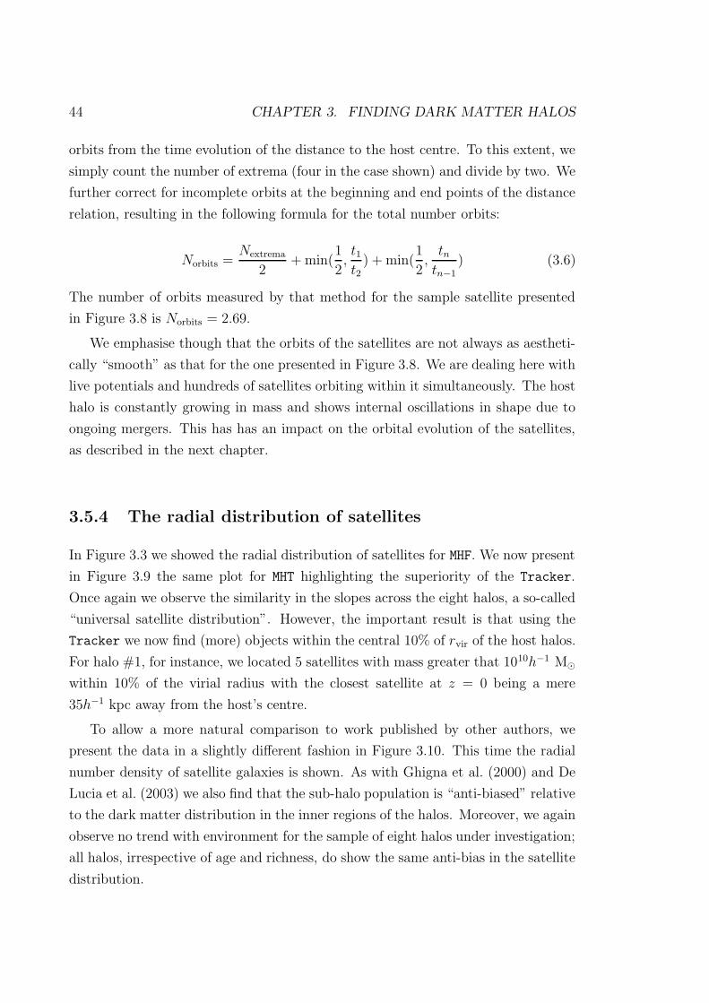
44 CHAPTER 3. FINDING DARK MATTER HALOS
orbits from the time evolution of the distance to the host centre. To this extent, we
simply count the number of extrema (four in the case shown) and divide by two. We
further correct for incomplete orbits at the beginning and end points of the distance
relation, resulting in the following formula for the total number orbits:
Norbits =Nextrema
2+ min(
1
2,t1t2
) + min(1
2,
tntn−1
) (3.6)
The number of orbits measured by that method for the sample satellite presented
in Figure 3.8 is Norbits = 2.69.
We emphasise though that the orbits of the satellites are not always as aestheti-
cally “smooth” as that for the one presented in Figure 3.8. We are dealing here with
live potentials and hundreds of satellites orbiting within it simultaneously. The host
halo is constantly growing in mass and shows internal oscillations in shape due to
ongoing mergers. This has has an impact on the orbital evolution of the satellites,
as described in the next chapter.
3.5.4 The radial distribution of satellites
In Figure 3.3 we showed the radial distribution of satellites for MHF. We now present
in Figure 3.9 the same plot for MHT highlighting the superiority of the Tracker.
Once again we observe the similarity in the slopes across the eight halos, a so-called
“universal satellite distribution”. However, the important result is that using the
Tracker we now find (more) objects within the central 10% of rvir of the host halos.
For halo #1, for instance, we located 5 satellites with mass greater that 1010h−1 M
within 10% of the virial radius with the closest satellite at z = 0 being a mere
35h−1 kpc away from the host’s centre.
To allow a more natural comparison to work published by other authors, we
present the data in a slightly different fashion in Figure 3.10. This time the radial
number density of satellite galaxies is shown. As with Ghigna et al. (2000) and De
Lucia et al. (2003) we also find that the sub-halo population is “anti-biased” relative
to the dark matter distribution in the inner regions of the halos. Moreover, we again
observe no trend with environment for the sample of eight halos under investigation;
all halos, irrespective of age and richness, do show the same anti-bias in the satellite
distribution.
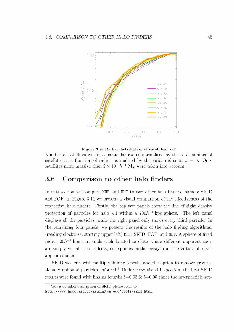
3.6. COMPARISON TO OTHER HALO FINDERS 45
Figure 3.9: Radial distribution of satellites: MHT
Number of satellites within a particular radius normalised by the total number ofsatellites as a function of radius normalised by the virial radius at z = 0. Onlysatellites more massive than 2 × 10¹⁰h−1 M were taken into account.
3.6 Comparison to other halo finders
In this section we compare MHF and MHT to two other halo finders, namely SKID
and FOF. In Figure 3.11 we present a visual comparison of the effectiveness of the
respective halo finders. Firstly, the top two panels show the line of sight density
projection of particles for halo #1 within a 700h−1 kpc sphere. The left panel
displays all the particles, while the right panel only shows every third particle. In
the remaining four panels, we present the results of the halo finding algorithms:
(reading clockwise, starting upper left) MHT, SKID, FOF, and MHF. A sphere of fixed
radius 20h−1 kpc surrounds each located satellite where different apparent sizes
are simply visualisation effects, i.e. spheres farther away from the virtual observer
appear smaller.
SKID was run with multiple linking lengths and the option to remove gravita-
tionally unbound particles enforced.3 Under close visual inspection, the best SKID
results were found with linking lengths b=0.03 & b=0.05 times the interparticle sep-
3For a detailed description of SKID please refer tohttp://www-hpcc.astro.washington.edu/tools/skid.html.

46 CHAPTER 3. FINDING DARK MATTER HALOS
Figure 3.10: Radial number density of satellites
Number density of satellites normalised by the average number of satellites per unitvolume as a function of radius normalised by the virial radius at z = 0. Onlysatellites more massive than 2 × 10¹⁰h−1 Mwere taken into account.
aration. The same values were taken for the FOF analysis. The results from the
analysis with linking length b=0.054 appear to be the most reliable ones and hence
are shown in Figure 3.11. We need to stress though that the analysis of the SKID
and FOF results can be further refined by combining various halo catalogues into a
tree as explained in, for instance, Ghigna et al. (2000). However, one of the benefits
our MLAPM halo finders is that neither requires any further input such as a linking
length or any other free parameter. Moreover, the latest version of MLAPM is capable
of performing the analysis “on-the-fly”. A visual inspection of Figure 3.11 indicates
that MHT provides the most complete halo list. Specifically, the Tracker found 53
satellites, the Finder found 32, SKID 33 and FOF 32 within the plotted spherical
region of diameter 1.4h−1 Mpc when restricting the analysis to objects with more
than 100 particles. Within the sets of satellites, there is of course considerable over-
lap. Essentially, each set of satellites found by MHF SKID, and FOF were subsets of
MHT. However, both SKID and FOF had halos that were spurious where this was not
4A linking length of b=0.05 expressed in terms of the interparticle separation translates into aphysical linking length of ∼6h
−1 kpc, which is roughly three times the force resolution.
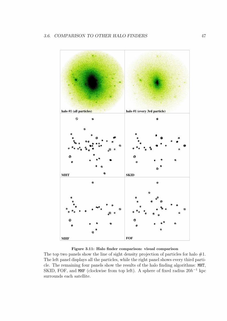
3.6. COMPARISON TO OTHER HALO FINDERS 47
halo #1 (all particles) halo #1 (every 3rd particle)
MHT SKID
MHF FOF
Figure 3.11: Halo finder comparison: visual comparison
The top two panels show the line of sight density projection of particles for halo #1.The left panel displays all the particles, while the right panel shows every third parti-cle. The remaining four panels show the results of the halo finding algorithms: MHT,SKID, FOF, and MHF (clockwise from top left). A sphere of fixed radius 20h−1 kpcsurrounds each satellite.
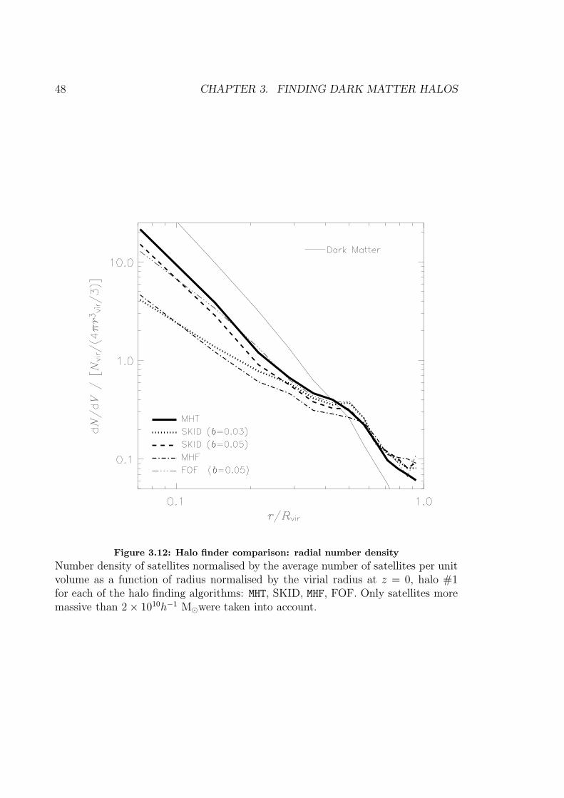
48 CHAPTER 3. FINDING DARK MATTER HALOS
Figure 3.12: Halo finder comparison: radial number density
Number density of satellites normalised by the average number of satellites per unitvolume as a function of radius normalised by the virial radius at z = 0, halo #1for each of the halo finding algorithms: MHT, SKID, MHF, FOF. Only satellites moremassive than 2 × 10¹⁰h−1 Mwere taken into account.
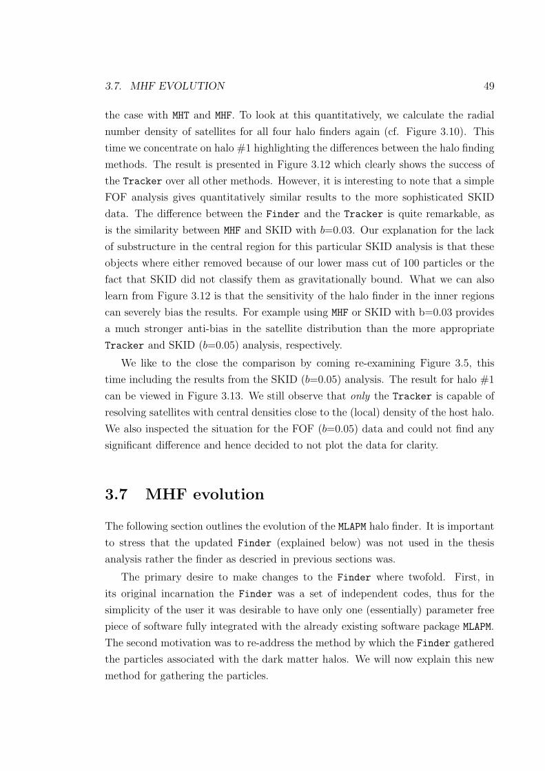
3.7. MHF EVOLUTION 49
the case with MHT and MHF. To look at this quantitatively, we calculate the radial
number density of satellites for all four halo finders again (cf. Figure 3.10). This
time we concentrate on halo #1 highlighting the differences between the halo finding
methods. The result is presented in Figure 3.12 which clearly shows the success of
the Tracker over all other methods. However, it is interesting to note that a simple
FOF analysis gives quantitatively similar results to the more sophisticated SKID
data. The difference between the Finder and the Tracker is quite remarkable, as
is the similarity between MHF and SKID with b=0.03. Our explanation for the lack
of substructure in the central region for this particular SKID analysis is that these
objects where either removed because of our lower mass cut of 100 particles or the
fact that SKID did not classify them as gravitationally bound. What we can also
learn from Figure 3.12 is that the sensitivity of the halo finder in the inner regions
can severely bias the results. For example using MHF or SKID with b=0.03 provides
a much stronger anti-bias in the satellite distribution than the more appropriate
Tracker and SKID (b=0.05) analysis, respectively.
We like to the close the comparison by coming re-examining Figure 3.5, this
time including the results from the SKID (b=0.05) analysis. The result for halo #1
can be viewed in Figure 3.13. We still observe that only the Tracker is capable of
resolving satellites with central densities close to the (local) density of the host halo.
We also inspected the situation for the FOF (b=0.05) data and could not find any
significant difference and hence decided to not plot the data for clarity.
3.7 MHF evolution
The following section outlines the evolution of the MLAPM halo finder. It is important
to stress that the updated Finder (explained below) was not used in the thesis
analysis rather the finder as descried in previous sections was.
The primary desire to make changes to the Finder where twofold. First, in
its original incarnation the Finder was a set of independent codes, thus for the
simplicity of the user it was desirable to have only one (essentially) parameter free
piece of software fully integrated with the already existing software package MLAPM.
The second motivation was to re-address the method by which the Finder gathered
the particles associated with the dark matter halos. We will now explain this new
method for gathering the particles.
50 CHAPTER 3. FINDING DARK MATTER HALOS
Figure 3.13: Halo finder comparison: central densities
Same as Figure 3.5, but this time comparing Tracker (diamonds) and Finder
(crosses) with the SKID, b=0.05 (triangles) analysis for halo #1.
3.7. MHF EVOLUTION 51
The central idea behind this new method for gathering halo particles is based on
the fact that when a cell is refined, the particles that are responsible of the refinement
of the cell are linked to that cell. Thus the particles are uniquely associated with the
cells and hence grids. Therefore, one can essentially “cut” of each of the branches
of the reconstructed “grid tree” and gather all the particles that are associated with
that branch/sub-halo.
However, when we cut the branches off in this manor we are only collecting the
particles associated with the sub-halo that are above the localised density of the
parent branch where the sub-halo is located. While this is fine for isolated halos
(which are cut at the virial density) for sub-halos it is less clear how to cut the
branch off.
Cutting sub-halos of at their branch density is essentially equivalent to collecting
the particles of the halo out to the upturn radius of the sub-halo (i.e. the radius at
which the background density begins to rise again). Although we have seen that sub-
halos sink within their host halo i.e. beyond this upturn radius (density cut) there
are particles still bound to the halos. To circumvent this difficulty we also collect all
the particles from the parent branch that are within half the distance to the next
closest more massive branch. We chose the next most massive branch because it
gives as an adaptive gathering radius, which is sensitive to the nature sub-halos i.e.
sub-halos are by definition smaller than their hosts. Further we gather particles not
simply from their immediate host branch (halo), but also from the host of their host
etc. if required.
Once we have done this we proceed to remove gravitationally unbound particles.
If a particle is found to be unbound we pass it to the host halo. The unbound
procedure is ordered in such a way that the smallest sub-(n)-sub-halos are checked
first for unbound particles.
Finally with the halo centres and the particles that belong to those halos gathered
we calculate the same canonical properties of the dark matter halos as previously
described.
The most significant difference between the previous Finder version and this
one is the way the particles are gathered. Previously the particles where simply
gathered in radial shells and each particle was not uniquely identified with a halo.
In this new method none of the particles are double counted because each particle
is uniquely assigned to a node.
The end result of the new Finder can be seen in Figure 3.14.

52 CHAPTER 3. FINDING DARK MATTER HALOS
Figure 3.14: The “new” halo finder
This figure shows the line-of-sight density projection of a halo early in its formation.In the top panel you can see the abundance of substructure. In the bottom panelhowever, the smaller substructure has been removed using the “new” MLAPM halofinder.
3.8. CONCLUSIONS 53
The precise details of the halo finding story, which is a story of carefully struc-
tured memory structures and complicated pointer arithmetic (this detailed story was
considered to terse for the reader) can be found by downloading the MLAPM source
and reading the detailed comments in the files ahf gridinfo.c & ahf halos.c.
3.8 Conclusions
Computational cosmology is not only limited by crucial factors such as the dynamical
range and the mass resolution, but also by its analysis tools. We emphasise, perhaps
obviously to most readers, that N -body codes simulating structure formation in the
Universe can only ever be as useful as their associated analysis tools allow.
In this chapter we presented two new methods for identifying gravitationally
bound objects in such simulations. Both methods are based upon the open source
adaptive mesh refinement code MLAPM (Knebe et al. 2001). They both exploit the
refinement hierarchy of said code and hence locate halos as well as halos-within-halos
with exactly the same accuracy as MLAPM simulates their evolution. We showed the
limitations of a simple snapshot analysis and how it can be overcome by taking into
account the whole history of each halo. Thus not restricting the halo finding algo-
rithm to just the spatial information but rather including the velocity information
as well, hence, using the full six-dimensional information available.
We showed that halo finding still possesses the inherent problem of overmerging
in the very central regions of the host. However, by tracking satellites rather than
identifying them at separate time snapshots of the simulation we learned that this
problem is not overmerging in the conventional sense. The objects are in fact present
and simulated properly, but their densities have insufficient contrast to be picked
up by a simple “finder”. Only when tracking them in time from (at best their very
own) formation time were we able to quantify their existence as close as 5% of rhostvir
to the cuspy centre. We do not intend to question the credibility of other (most
excellent) halo finders such as SKID though. We rather pointed out that the results
in the central region are subject to subtleties that can be most easily avoided by
tracking satellites.
It has recently been pointed out by Taylor et al. (2003) that the radial distri-
bution of the Milky Way’s satellite galaxies does not reconcile with the predictions
of semi-analytical models of galaxy formation and cosmological simulations, respec-
54 CHAPTER 3. FINDING DARK MATTER HALOS
tively, which has been confirmed by Kravtsov et al. (2004). Even though there is
quite a prominent substructure population in the simulations it is mostly clustered
in the outer regions of the host whereas the Milky Way satellites are preferentially
found closer in. It remains unclear if this poses a new challenge to the CDM struc-
ture formation scenario or simply reflects what we presented in this study. Namely,
identifying substructure halos that lie close to the centre of the host is intrinsically
challenging and might be overcome by actually tracking the satellites rather than
finding them.
We further increase the statistics to suggest that anti-bias of the satellite distri-
bution is a common property of the satellite distribution, perhaps even universal.
However, this antibias is still most likely a relic of numerical overmerging. A con-
vergence study for the satellite populations is critical in resolving this issue and
reconciling the lensing observations. However, one very interesting result is the con-
tinued self-similarity in the dark matter distribution, the satellite radial distribution
is common, once again perhaps “”universal” even though the number of substruc-
ture satellites changes, reminiscent of the universal density profile of the underlying
host.
Finally, we updated the development of the MHF a quicker and cleaner implemen-
tation that is open source.
Chapter 4
The dynamics of substructure
“The dynamics of capitalism is postponement of
enjoyment to the constantly postponed future.”
- Norman O. Brown
4.1 Introduction
As we have seen within CDM structure forms hierarchically, whereby small objects
(sub-halos) form first and subsequently merge to progressively form larger objects
(White & Reese 1978; Davis et al. 1985). Thus the dynamical properties of the
accreting sub-halos reflect the formation of the underlying host. Hence, it is im-
perative to understand the orbital evolution of these objects and how they deviate
from the background dark matter distribution. The first few chapters of this thesis
introduced the tools for investigating these sub-halos, we now investigate the general
properties of these accreting sub-halos analysing in detail their temporal and spatial
properties.
To date, typical sub-halos (satellite) properties such as orbital parameters and
mass loss due to tidal interactions with their host halo have primarily been investi-
gated using static potentials for the dark matter host halo (e.g. Johnston et al. 1996;
Hayashi et al. 2003). We stress that each of these studies have provided invalu-
able insights into the physical processes involved in satellite disruption; our goal
is, however, to augment these studies by relaxing the assumption of a static host
potential, in deference to the fact that realistic dark matter halos are not necessarily
axis-symmetric or time independent. As we saw in Chapter 2 halos are constantly
55
56 CHAPTER 4. THE DYNAMICS OF SUBSTRUCTURE
growing in mass through slow accretion and violent mergers, varying in dynamical
relaxation and possessing triaxial shapes.
While a self-consistent cosmological modelling of both hosts and satellites has
long been recognised as optimal, the required mass and force resolution can be
difficult to accommodate due to computational costs, hence the use of static host
potentials in most previous studies.
The first fully self-consistent simulations targeting the subject were performed
by Tormen (1997) and Tormen et al. (1998). Both studies were landmark efforts, but
lacked the temporal, spatial, and mass resolution necessary to explore a wide range
of environmental effects. Unable to follow the satellite distribution within the host’s
virial radius, satellites were instead tracked only up to and including the point of
“accretion”. This allowed an analysis of the in-fall pattern, rather than the orbital
evolution of the satellites. Ghigna et al. (1998) also investigated the dynamics of
satellite galaxies in live dark matter host halos. Although greatly increasing the mass
and spatial resolution, they still lacked the temporal resolution to explicitly track
the satellite orbits. Instead, the orbits were approximated using a spherical static
potential. More recently, Taffoni et al. (2003) used N -body simulations coupled with
semi-analytical tools to explore the evolution of dark matter satellites inside more
massive halos. However, they focus their efforts on the interplay between dynamical
friction and tidal mass loss in determining the final fate of the satellites.
As we have seen in previous chapters our suite of simulations has the required
resolution to follow the satellites even within the very central regions of the host
potential (≥5–10% of the virial radius) and the time resolution to resolve the satellite
dynamics with excellent accuracy (∆t ≈170 Myrs). Hence, we have excellent data
possessing high spatial, mass, and temporal resolution which uniquely enables us to
investigate the evolution of sub-halos and their relation to their Hosts.
The outline of the chapter is as follows. In the first section we continue our
analysis from the previous chapter, investigating now the satellite populations of the
host halos and investigate their global properties such as total mass. In Section 4.3
we discuss the internal structure of the satellites. In Section 4.4 we take a detailed
look at the satellite orbital parameters. We then investigate the kinematic properties
of the dark matter halos and satellites in Section 4.5 and finish with our summary
and conclusions in Section 4.6.
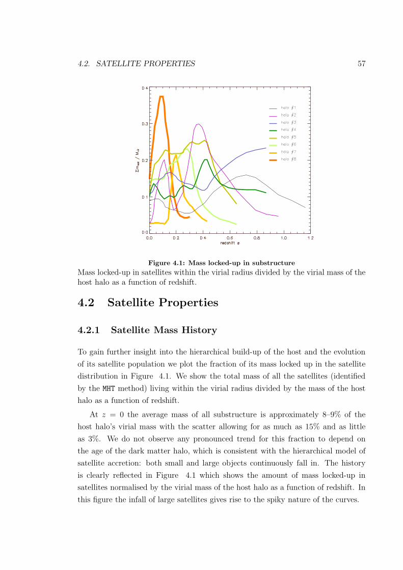
4.2. SATELLITE PROPERTIES 57
Figure 4.1: Mass locked-up in substructure
Mass locked-up in satellites within the virial radius divided by the virial mass of thehost halo as a function of redshift.
4.2 Satellite Properties
4.2.1 Satellite Mass History
To gain further insight into the hierarchical build-up of the host and the evolution
of its satellite population we plot the fraction of its mass locked up in the satellite
distribution in Figure 4.1. We show the total mass of all the satellites (identified
by the MHT method) living within the virial radius divided by the mass of the host
halo as a function of redshift.
At z = 0 the average mass of all substructure is approximately 8–9% of the
host halo’s virial mass with the scatter allowing for as much as 15% and as little
as 3%. We do not observe any pronounced trend for this fraction to depend on
the age of the dark matter halo, which is consistent with the hierarchical model of
satellite accretion: both small and large objects continuously fall in. The history
is clearly reflected in Figure 4.1 which shows the amount of mass locked-up in
satellites normalised by the virial mass of the host halo as a function of redshift. In
this figure the infall of large satellites gives rise to the spiky nature of the curves.
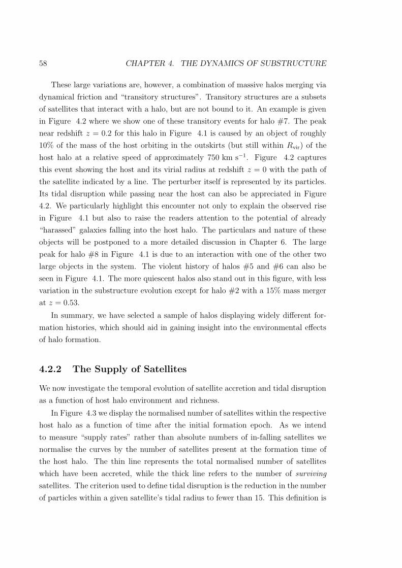
58 CHAPTER 4. THE DYNAMICS OF SUBSTRUCTURE
These large variations are, however, a combination of massive halos merging via
dynamical friction and “transitory structures”. Transitory structures are a subsets
of satellites that interact with a halo, but are not bound to it. An example is given
in Figure 4.2 where we show one of these transitory events for halo #7. The peak
near redshift z = 0.2 for this halo in Figure 4.1 is caused by an object of roughly
10% of the mass of the host orbiting in the outskirts (but still within Rvir) of the
host halo at a relative speed of approximately 750 km s−1. Figure 4.2 captures
this event showing the host and its virial radius at redshift z = 0 with the path of
the satellite indicated by a line. The perturber itself is represented by its particles.
Its tidal disruption while passing near the host can also be appreciated in Figure
4.2. We particularly highlight this encounter not only to explain the observed rise
in Figure 4.1 but also to raise the readers attention to the potential of already
“harassed” galaxies falling into the host halo. The particulars and nature of these
objects will be postponed to a more detailed discussion in Chapter 6. The large
peak for halo #8 in Figure 4.1 is due to an interaction with one of the other two
large objects in the system. The violent history of halos #5 and #6 can also be
seen in Figure 4.1. The more quiescent halos also stand out in this figure, with less
variation in the substructure evolution except for halo #2 with a 15% mass merger
at z = 0.53.
In summary, we have selected a sample of halos displaying widely different for-
mation histories, which should aid in gaining insight into the environmental effects
of halo formation.
4.2.2 The Supply of Satellites
We now investigate the temporal evolution of satellite accretion and tidal disruption
as a function of host halo environment and richness.
In Figure 4.3 we display the normalised number of satellites within the respective
host halo as a function of time after the initial formation epoch. As we intend
to measure “supply rates” rather than absolute numbers of in-falling satellites we
normalise the curves by the number of satellites present at the formation time of
the host halo. The thin line represents the total normalised number of satellites
which have been accreted, while the thick line refers to the number of surviving
satellites. The criterion used to define tidal disruption is the reduction in the number
of particles within a given satellite’s tidal radius to fewer than 15. This definition is
4.2. SATELLITE PROPERTIES 59
Figure 4.2: Backsplash galaxy
This figure shows a satellite of mass 10% the host halo that is responsible for thejump in the host’s mass accretion history. The host halo (halo # 7) is plotted asa line of sight density projection using every 3rd particle, whereas the satellite isrepresented by all its particles without a density map. The satellite enters the haloat z = 0.25 (lower right) and leaves again around z = 0 with the thin line indicatingits orbit. The sphere shows the virial radius of the halo at z = 0 and the relativevelocities of the two objects is 750 km s−1.
60 CHAPTER 4. THE DYNAMICS OF SUBSTRUCTURE
somewhat arbitrary, although ultimately based upon the numerical resolution. For
a more detailed discussion please refer to the previous chapter.
The increase in the total number of satellites (thin curve) reflects the “richness”
of the environment around the halo: halos with a steep slope benefit from a constant
supply of satellite galaxies where as hosts that only show a mild increase draw upon
a pool of fewer satellites in their immediate vicinity. This is illustrated by the case
of halo #1 which lies in a particularly rich environment in which several filaments
intersect (cf. Figure 4.4). As a consequence, it accretes a total of nearly five
times the initial number of satellites while simultaneously showing a high satellite
disruption rate. The case of halo #3 is similar, but less extreme. Halos #7 and
#8, by contrast, experience only moderate in-fall, and in these halos nearly all the
satellites survive. The situation is illustrated for halos #1 and #8 in Figure 4.4 &
4.5 respectively, which shows the orbital paths followed by all the satellites from the
formation epoch up to the present day. In Figure 4.4 we clearly see the filament
”arms” that feed halo #1 and how the satellites spiral into the dark matter halo.
The filaments are helical because they consist of smaller satellites orbiting a larger
host that is falling into the massive host halo. The small but rapid rise in the
satellite in-fall for halo #1 (Figure 4.3) is caused by a group of satellites falling into
the halo for the first time. In Figure 4.5 we feature halo #8; in contrast to halo #1,
halo #8 was formed in a relatively isolated region which saw a rapid collapse. We
can, however, confirm that even though the satellite accretion rate in halo #8 is far
less the mass of the infalling objects is much higher. This is derived from the fact
that halo #8 acquires half its mass by digesting those few satellites in a time span
of approximately 3 Gyrs (cf. Figure 4.1). We note though that there also exists
a significant age difference between halo #1 and #8; this explains why halo #8
satellites are traced for a shorter time leading to the “shorter” lines in Figure ??.
However, there still exist noticeable differences in the satellite accretion curves for
halos #1 and #8 (cf. Figure 4.3) when restricting halo #1 to the first 3.5 Gyrs of
its existence.
We define the substructure “richness” as the ratio of the final to initial number
of satellites, and list its value for each of the eight halos in Table 4.1.
The number of surviving satellites is not directly correlated with the richness, but
rather to the orbital characteristics of the accreted satellites, as we will demonstrate
in detail below. In general, the accreted satellites are not immediately disrupted,
but are progressively destroyed over time.

4.2. SATELLITE PROPERTIES 61
Figure 4.3: Number of satellites within the virial radius as a function of redshift
Number of satellites within the virial radius of their respective host as a functionof redshift. The thin line is the total number of satellites that have fallen into thehost whereas the thick line shows the number of surviving satellites. Both lines arenormalised to the total number of satellites at zform.
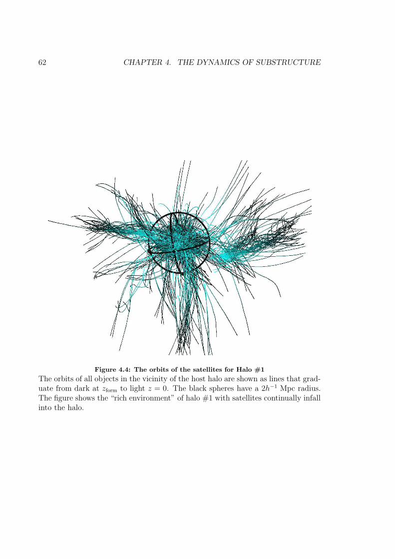
62 CHAPTER 4. THE DYNAMICS OF SUBSTRUCTURE
Figure 4.4: The orbits of the satellites for Halo #1
The orbits of all objects in the vicinity of the host halo are shown as lines that grad-uate from dark at zform to light z = 0. The black spheres have a 2h−1 Mpc radius.The figure shows the “rich environment” of halo #1 with satellites continually infallinto the halo.

4.2. SATELLITE PROPERTIES 63
Figure 4.5: The same as Figure 4.4 but this time showing the more isolated halo #8.Halo #8 saw an early rapid infall of essentially all its associated satellite substructurethen little latter on.
64 CHAPTER 4. THE DYNAMICS OF SUBSTRUCTURE
To further investigate the link between satellite disruption and satellite in-fall we
calculate the ratio of disrupted (or “dead”) satellites to the total number of satellites
that fall into the host halo. The result is presented in Figure 4.6. It is now possible
to interpret the slope of this figure as the “rate of disruption” of satellite galaxies.
For all halos this disruption rate (i.e. slope) is very similar. There seems to be
no strongly pronounced correlation with either mass, environment or age. In this
respect, the destruction rate of satellite galaxies appears to be “common” in CDM
halos. However, there also appears to be a (marginal) trend that host mass is related
to the ability to disrupt satellites (within the limited mass range presented here).
This can be seen explicitly for halos #1 and #3: #1 destroys its satellites more
efficiently than #3 and is also the more massive of the two. However, these halos
also have a large difference in triaxiality (refer to Table 4.1). Conversely, as halo #3
is comparable in mass to halo #4 with a strikingly similar satellite destruction rate.
But as halo #3 and #4 are close in triaxiality, we rather suspect the disruption rate
to correlate with mass than with triaxiality. However, this correlation - if in fact
correct - must also have significant scatter, as the most massive halo (#8) shows
the lowest destruction rate. This might be linked to the environment and supply of
new satellites, respectively.
4.2.3 Summary of Host Halos and Satellite properties
Table 4.1 summarises the additional basic properties of our halos and their environ-
ments, illustrating the variety of richness and satellite number. Note, an applied
mass-cut of 2 × 10¹⁰h−1 M (corresponding to 100 particles) was used, which ex-
plains the rather ’low’ number for Nsat(<rvir) in Table 4.1. Further, this fixed mass
cut explains the variation in the number of satellites from halo to halo.
4.3 Density Profiles of Satellites
For field galaxies in cosmological simulations there is the well know relationship
between rmax, the point where the rotation curve of the satellite galaxy peaks and
the scale radius rs (as defined in Eq. (4.1)) (Bullock 2001). In this section we aim
to verify this relation for substructure halos, which on analytical grounds should be
of the order rmax ≈ rs.
To verify this analytical relation we rather use the cumulative density profile

4.3. DENSITY PROFILES OF SATELLITES 65
Figure 4.6: The rate of satellite disruption
The ratio of “disrupted” satellites to the total number of satellites for satelliteswithin the virial radius of their respective host, as a function of time, where zeroage is the formation time of the halo.
Table 4.1: Additoinal properties of the eight host dark matter halos.
Halo Nsat(<Rvir) richness
# 1 158 4.7# 2 63 3.1# 3 87 4.3# 4 57 2.9# 5 175 3.6# 6 85 3.2# 7 59 1.9# 8 251 2.8
66 CHAPTER 4. THE DYNAMICS OF SUBSTRUCTURE
ρ(< r) than the differential ρ(r); for (sub-)halos containing orders of magnitude
fewer particles than the host this leads to a more smooth profile and hence a more
stable fit to an analytical function.
ρcum(r) =M(< r)
4πr3/3=
ρsr3s
r(rs + r)2(4.1)
where rs is our scale radius used to calculate the concentration c = rvir/rs. Navarro
(1997) used the differential density profile
ρNFW(r) =dM(r)
dV=
ρNFWs R3
s
r(Rs + r)2(4.2)
where is rs again is used to define the concentration cNFW = rvir/Rs of the halo.
We are interested in a relation between our scale radius rs and the maximum of the
circular rotation curve rmax as presented for our sub-halo populations in Figure 4.7.
Therefore using
v2circ =
GM(< r)
r(4.3)
together with Eq. (4.1) gives
v2circ =
4πGrρsr3s
3(rs + r)2(4.4)
We obtain the maximum of vcirc by differentiating it with respects to r
dvcirc
dr=
1
2vcirc
4πGr3s
3(rs + r)2
(
1 − 2r
rs + r
)
(4.5)
and setting it to zero. Simple algebra then reveals the relation
rs = rmax (4.6)
To verify this relation we plot rs versus rmax in Figure 4.7. We find that this
relation holds for all our satellite galaxies with very little scatter. The solid line
is the one-to-one relation with the dashed lines showing rs = 2rmax (upper) and
rs = 0.5rmax (lower).
Thus as for satellite galaxies in the ’field’ this same relationship holds for galaxies
within clusters. Although it is important to verify this relationship with higher
resolution simulations since the inner profiles of sub-halos are challenging to resolve.

4.3. DENSITY PROFILES OF SATELLITES 67
Figure 4.7: Density Profiles of Substructure Halos
We plot the relation between scale radius rs defined in Eq. (4.1) and the positionof the maximum of the rotation curve. Both of these values are normalised by thehosts virial radius.
68 CHAPTER 4. THE DYNAMICS OF SUBSTRUCTURE
4.4 Satellite Orbital Parameters
We now turn to the detailed analysis of the evolution of satellite galaxies. In the
following subsections we investigate their lifetimes, orbital parameters, and derive
relevant correlations and relations.
4.4.1 Number of Satellite Orbits
In Figure 4.8 we show the distribution of the number of orbits for both surviving
satellites (thick lines) and disrupted satellites (thin lines) at redshift z = 0.
For the satellites that survived until z = 0 the distribution peaks at or near one
orbit for each of the eight host halos. More than 70% of the satellites have had at
least one full orbit with some having as many as four, therefore making a study of
the satellite dynamics valid. The length of the tail to the right of the peak at one
orbit is somewhat correlated with the age of the dark matter halo. Further, the peak
is more pronounced in the younger halos. However, halos #1 and #3 both show
distinctive peaks at one orbit which relates to the richness of environment given in
Table 4.1, rather than the age, as satellites are continuously falling in.
The interpretation of the distribution for the disrupted satellites is more inter-
esting. We note that these orbits are determined by mass-less tracer particles placed
at the last credible centre of the satellite before disruption. The distributions are
generally “flatter” with the most prominent peak near zero orbits. One explana-
tion for such a distribution is that the in-falling satellites are being disrupted before
completing one orbit. This suggests that satellites contributing to this bin in the
distribution are very massive and rapidly decay via dynamical friction. Having said
that, we emphasize that this interpretation may be somewhat simplistic. All satel-
lites were identified at zform and we do not have an indication as to how long the
satellites had already existed within the host’s progenitor prior to that redshift.
Therefore, (massive) satellites that had already been orbiting within the progenitor
would be the first to be disrupted, giving this biased result. Another small contri-
bution to this bin is from the sub-substructure. As seen in Figure 4.4 the systems
of substructure are spiralling into the dark matter halo, thus the sub-structure is
being destroyed in its very own (sub-)host before completing a full orbit. Regardless
of this “zero orbit” peak, most of the disrupted satellites complete at least the same
number of orbits as the ones which survive to z = 0.
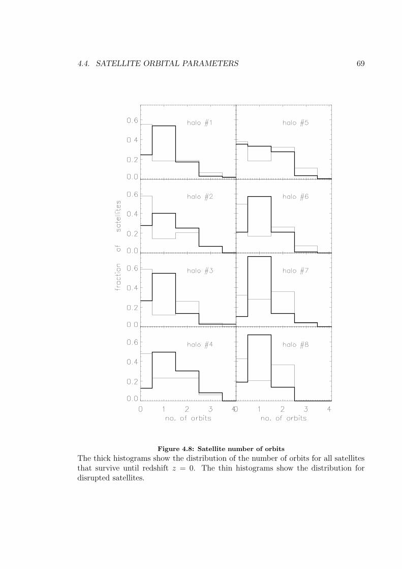
4.4. SATELLITE ORBITAL PARAMETERS 69
Figure 4.8: Satellite number of orbits
The thick histograms show the distribution of the number of orbits for all satellitesthat survive until redshift z = 0. The thin histograms show the distribution fordisrupted satellites.
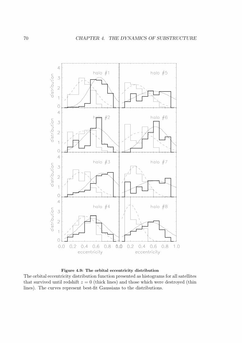
70 CHAPTER 4. THE DYNAMICS OF SUBSTRUCTURE
Figure 4.9: The orbital eccentricity distribution
The orbital eccentricity distribution function presented as histograms for all satellitesthat survived until redshift z = 0 (thick lines) and those which were destroyed (thinlines). The curves represent best-fit Gaussians to the distributions.
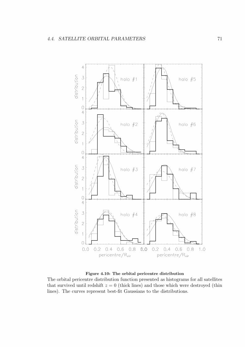
4.4. SATELLITE ORBITAL PARAMETERS 71
Figure 4.10: The orbital pericentre distribution
The orbital pericentre distribution function presented as histograms for all satellitesthat survived until redshift z = 0 (thick lines) and those which were destroyed (thinlines). The curves represent best-fit Gaussians to the distributions.

72 CHAPTER 4. THE DYNAMICS OF SUBSTRUCTURE
4.4.2 Orbital Eccentricity and Pericentres
As previously stated, we define eccentricity as
e = 1 − p
a, (4.7)
where the pericentre p and apocentre a distances were those last measured in the
satellite’s (or the tracer particle’s) orbit. Using this definition we show in Figure 4.9
the distribution of the orbital eccentricity e for both live (thick lines) and disrupted
satellites (thin lines). Further, we fit a Gaussian
P (e) =1√
2πσ2e−
(e−e0)2
2σ2 (4.8)
to the distributions (solid curves for live and dashed lines for disrupted satellites).
From this fit the peak orbital eccentricity for the eight halos has an average of 〈e0〉 =
0.61 with an average standard deviation of 〈σ〉 = 0.19. We do not observe again
any correlation of peak position and width of the distribution with environment,
age, host history or richness, even though σ appears to be larger for the younger
dark matter halos. It is interesting to note that if we stack the data from the eight
halos together and then separate the satellite population into differing mass bins
we see little variation. This common behaviour still holds and probably reflects the
scale free nature of gravity and hierarchical structure formation in CDM models.
The disrupted satellites, however, have a different distribution, almost mirroring
the survivors about the e = 0.5-axes, with the peak eccentricity near 〈ed0〉 = 0.34
and a dispersion of 〈σd〉 = 0.16. Thus, the destroyed satellites were preferentially
on more circular orbits.
The pericentre distributions provide additional insight into the nature of the
orbits of the disrupted satellites. The result for redshift z = 0 can be seen in Fig-
ure 4.10 where p has been normalised by the virial radius of the host. Again, live
satellites are represented as thick lines and disrupted ones as thin lines. A strik-
ing characteristic of these distributions is again the similarity between the halos.
Moreover, we also observe a similarity in the distribution for the live and disrupted
satellites. This is emphasised particularly by the best-fit Gaussians to the distri-
butions. The maximum peak lies at 35% of the virial radius for live satellites with
a mean dispersion of 〈σ〉 = 0.12 as opposed to 31% of Rvir for the disrupted ones
with a dispersion of 〈σd〉 = 0.11. Unlike eccentricity, the pericentre distribution rises

4.4. SATELLITE ORBITAL PARAMETERS 73
quickly towards the peak and falls off moderately to the outer parts of the host halo.
We already noted the lack of correlation with mass, age, environment and richness,
but there is, however, a mild dependence on the state (live or dead) of the satellite
as disrupted satellites appear to have had marginally nearer excursions towards the
host centre. When we stack the data from the eight halos and separate into differing
satellite mass bins we again see little variation.
In summary the difference between live and disrupted satellites lies primarily
in the eccentricity distribution. Disrupted satellites seem to be on more circular
orbits. Since the disrupted satellites have similar pericentres to those which survive
their circular nature means that they spend more time in the deeper regions of the
potential well. Hence, they experience stronger tidal forces for longer periods, and
are thus disrupted more easily.
We close this subsection with an examination of the pericentre-eccentricity rela-
tion (Figure 4.11). The crosses represent the satellites that survived until redshift
z = 0, while the diamonds represent the disrupted satellites. Although many of
the features seen here are also seen in Figure 4.9 and Figure 4.10, there are two
additional ones which we will comment on now.
One such feature is the bimodality in the satellite distribution of halo # 1.
In this Figure there seems to be two distinct (live and dead) satellite populations
orbiting within the dark matter halo. As we saw, particularly in Figure 4.4, this
dark matter halo lies in a rich area being fed by (at least) two filaments. Perhaps
these two satellite populations are a remnant of the filamentary large-scale structure
surrounding the host? If that is true, it is interesting that the satellites still maintain
their dynamical distinctiveness after several orbits.
In addition there appears to be a distinct population of satellites with an ex-
tremely tight (anti-)correlation between eccentricities e ≈ 0.6 − 0.9 and pericentres
p ≈ 0.3−0.8 in many halos. Upon detailed investigation these satellites were identi-
fied to have completed one orbit and were entering the halo for the first time. This is
consistent with the notion of the satellites in-falling on radial orbits. We investigate
this point in the next section, namely the evolution of eccentricity.
4.4.3 Evolution of Eccentricity
In the previous section we considered the orbital characteristics of the satellites at
redshift z = 0. We now investigate the evolution of the orbital eccentricities of the

74 CHAPTER 4. THE DYNAMICS OF SUBSTRUCTURE
Figure 4.11: Satellite eccentricity vs pericentre
We plot the satellite eccentricity against pericentre normalised by the virial radiusof the host. The crosses represent the satellites that survived until z = 0 while thediamonds represent the disrupted satellites.

4.4. SATELLITE ORBITAL PARAMETERS 75
Figure 4.12: Evolution of orbital eccentricity
The final orbital eccentricity plotted against the number of orbits completed foreach surviving satellite (crosses). The histogram shows the averaged eccentricity(see text for details).
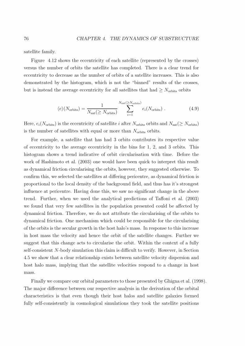
76 CHAPTER 4. THE DYNAMICS OF SUBSTRUCTURE
satellite family.
Figure 4.12 shows the eccentricity of each satellite (represented by the crosses)
versus the number of orbits the satellite has completed. There is a clear trend for
eccentricity to decrease as the number of orbits of a satellite increases. This is also
demonstrated by the histogram, which is not the “binned” results of the crosses,
but is instead the average eccentricity for all satellites that had ≥ Norbits orbits
〈e〉(Norbits) =1
Nsat(≥ Norbits)
Nsat(≥Norbits)∑
i=1
ei(Norbits) . (4.9)
Here, ei(Norbits) is the eccentricity of satellite i after Norbits orbits and Nsat(≥ Norbits)
is the number of satellites with equal or more than Norbits orbits.
For example, a satellite that has had 3 orbits contributes its respective value
of eccentricity to the average eccentricity in the bins for 1, 2, and 3 orbits. This
histogram shows a trend indicative of orbit circularisation with time. Before the
work of Hashimoto et al. (2003) one would have been quick to interpret this result
as dynamical friction circularising the orbits, however, they suggested otherwise. To
confirm this, we selected the satellites at differing pericentre, as dynamical friction is
proportional to the local density of the background field, and thus has it’s strongest
influence at pericentre. Having done this, we saw no significant change in the above
trend. Further, when we used the analytical predictions of Taffoni et al. (2003)
we found that very few satellites in the population presented could be affected by
dynamical friction. Therefore, we do not attribute the circularising of the orbits to
dynamical friction. One mechanism which could be responsible for the circularising
of the orbits is the secular growth in the host halo’s mass. In response to this increase
in host mass the velocity and hence the orbit of the satellite changes. Further we
suggest that this change acts to circularise the orbit. Within the context of a fully
self-consistent N -body simulation this claim is difficult to verify. However, in Section
4.5 we show that a clear relationship exists between satellite velocity dispersion and
host halo mass, implying that the satellite velocities respond to a change in host
mass.
Finally we compare our orbital parameters to those presented by Ghigna et al. (1998).
The major difference between our respective analysis in the derivation of the orbital
characteristics is that even though their host halos and satellite galaxies formed
fully self-consistently in cosmological simulations they took the satellite positions

4.5. HOST AND SATELLITE KINEMATICS 77
and velocities and evolved them in a static spherical potential in order to obtain
orbital characteristics. Ghigna et al. found that the satellites on radial orbits were
more likely to be disrupted than those on circular orbits because they penetrate
further into the dark matter halo potential well. In addition, radial orbits were
quite common and circular orbits quite rare in their simulations. The average ratio
of apocentre:pericentre in their outputs was 6:1, with nearly 25% of the halos on
orbits with ratios in excess of 10:1. In our language this 6:1 ratio equates to an ec-
centricity of ∼ 0.83. Hence, the Ghigna et al. satellite orbits were considerably more
radial than ours. We can not reconcile this discrepancy through dynamical friction
arguments. However, it could potentially be explained by the lack of a live halo.
This explanation correlates with our previous finding in Section 4.4 for a recently
in-falling satellite population. This latter population constitute a distinct subpop-
ulation with a strong (anti-)correlation in Figure 4.11 and an average eccentricity
of ∼ 0.8, quite similar to the result of Ghigna et al. .
4.4.4 Circularity of Orbits
Another way to measure the circularity of the orbits can be written
λ =Jsat(E)
Jcirc(E)
(4.10)
where λ is the ratio between the actual angular momentum of the satellite Jsat and
the angular momentum of a circular orbit Jcirc with the same energy E.
The correlation of λ with the the orbital eccentricity defined in Eq. (4.7) is
presented in Figure 4.13 for all satellites that had at least one full orbit at redshift
z = 0. The solid lines are upper limits given by the assumption that both satellite
and host halo are point masses. For a derivation of this relation please refer to the
Appendix.
We observe that most of the satellites follow the trend indicated by the analytical
estimate showing that low-eccentricity satellites are in fact on more circular orbits.
However, the trend is only suggestive but not strong with a significant scatter making
it difficult to substitute one measure for the other.

78 CHAPTER 4. THE DYNAMICS OF SUBSTRUCTURE
Figure 4.13: Circularity vs orbital eccentricity
Circularity as a function of orbital eccentricity. Only satellites with at least one fullorbit are considered and the solid line marks the 1:1 correlation.
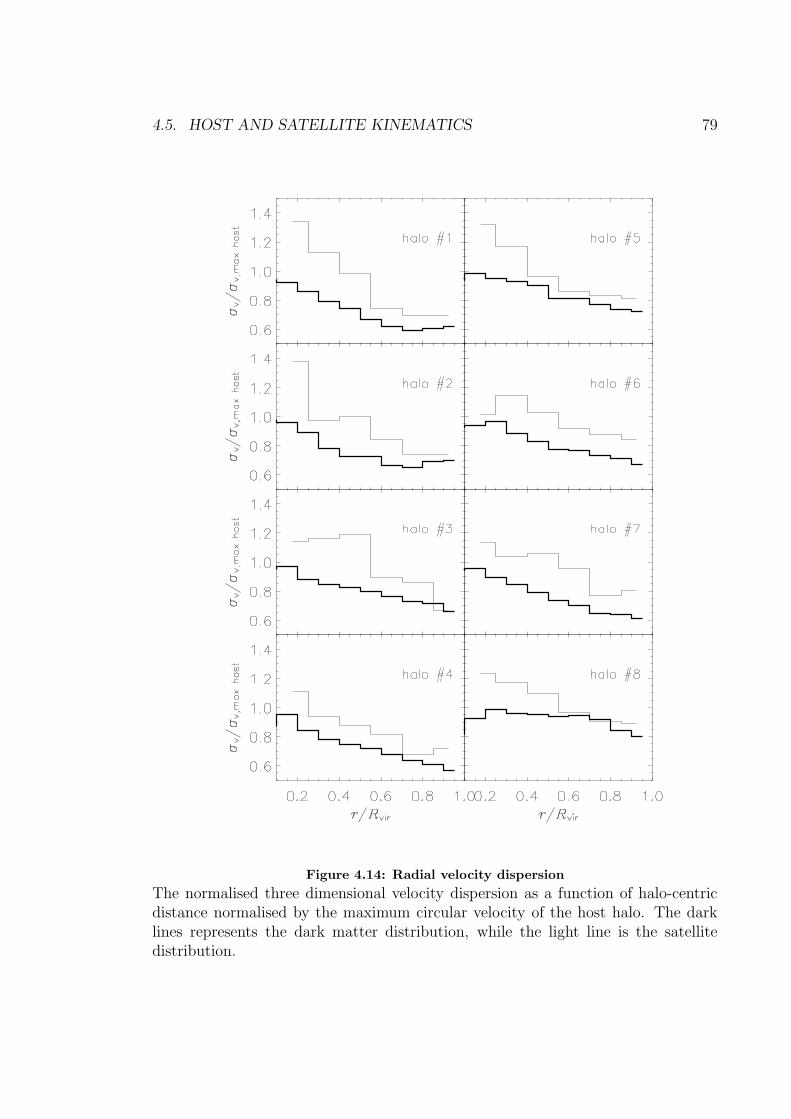
4.5. HOST AND SATELLITE KINEMATICS 79
Figure 4.14: Radial velocity dispersion
The normalised three dimensional velocity dispersion as a function of halo-centricdistance normalised by the maximum circular velocity of the host halo. The darklines represents the dark matter distribution, while the light line is the satellitedistribution.
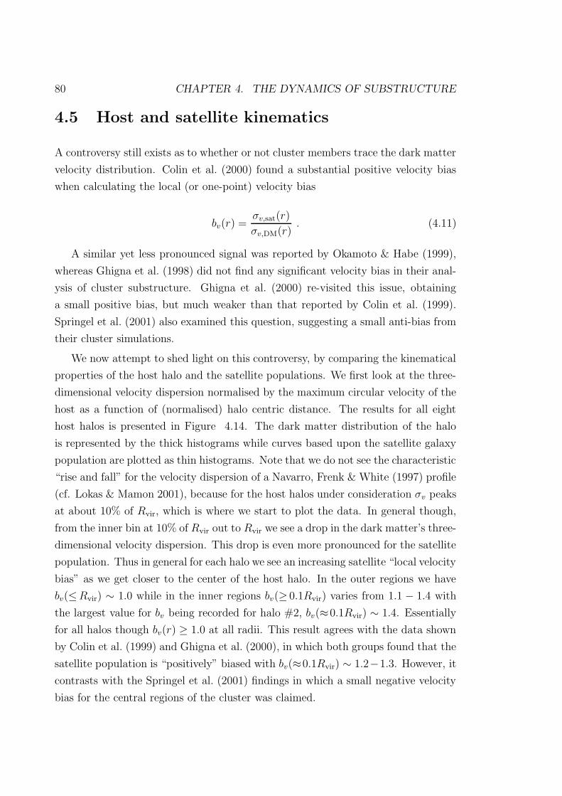
80 CHAPTER 4. THE DYNAMICS OF SUBSTRUCTURE
4.5 Host and satellite kinematics
A controversy still exists as to whether or not cluster members trace the dark matter
velocity distribution. Colin et al. (2000) found a substantial positive velocity bias
when calculating the local (or one-point) velocity bias
bv(r) =σv,sat(r)
σv,DM(r). (4.11)
A similar yet less pronounced signal was reported by Okamoto & Habe (1999),
whereas Ghigna et al. (1998) did not find any significant velocity bias in their anal-
ysis of cluster substructure. Ghigna et al. (2000) re-visited this issue, obtaining
a small positive bias, but much weaker than that reported by Colin et al. (1999).
Springel et al. (2001) also examined this question, suggesting a small anti-bias from
their cluster simulations.
We now attempt to shed light on this controversy, by comparing the kinematical
properties of the host halo and the satellite populations. We first look at the three-
dimensional velocity dispersion normalised by the maximum circular velocity of the
host as a function of (normalised) halo centric distance. The results for all eight
host halos is presented in Figure 4.14. The dark matter distribution of the halo
is represented by the thick histograms while curves based upon the satellite galaxy
population are plotted as thin histograms. Note that we do not see the characteristic
“rise and fall” for the velocity dispersion of a Navarro, Frenk & White (1997) profile
(cf. Lokas & Mamon 2001), because for the host halos under consideration σv peaks
at about 10% of Rvir, which is where we start to plot the data. In general though,
from the inner bin at 10% of Rvir out to Rvir we see a drop in the dark matter’s three-
dimensional velocity dispersion. This drop is even more pronounced for the satellite
population. Thus in general for each halo we see an increasing satellite “local velocity
bias” as we get closer to the center of the host halo. In the outer regions we have
bv(≤Rvir) ∼ 1.0 while in the inner regions bv(≥ 0.1Rvir) varies from 1.1 − 1.4 with
the largest value for bv being recorded for halo #2, bv(≈0.1Rvir) ∼ 1.4. Essentially
for all halos though bv(r) ≥ 1.0 at all radii. This result agrees with the data shown
by Colin et al. (1999) and Ghigna et al. (2000), in which both groups found that the
satellite population is “positively” biased with bv(≈0.1Rvir) ∼ 1.2−1.3. However, it
contrasts with the Springel et al. (2001) findings in which a small negative velocity
bias for the central regions of the cluster was claimed.

4.5. HOST AND SATELLITE KINEMATICS 81
Table 4.2: The global velocity bias for the eight host dark matter halos, within thevirial radius.
halo σv,halo σv,sats bv,global bNorbits≥1v,global
# 1 1140 1077 1.12 1.01# 2 887 811 1.07 1.01# 3 900 834 1.09 0.98# 4 789 729 1.06 0.99# 5 1170 1168 1.08 0.98# 6 857 807 1.12 1.03# 7 811 852 1.19 1.13# 8 1067 1119 1.09 1.02
There is no discernible relationship between the eccentricity distribution (cf.
Figure 4.9) and the bias seen in Figure 4.14; however, there is sufficient orbital dis-
tribution variation to accommodate for the variation in the bias. Improved statistics
will be needed to decouple the detailed variations. However, we have shown that
the velocity bias has the same basic shape for all eight halos, strengthening the case
that this is a general characteristic of the satellite population.
Using all the dark matter particles and satellite galaxies within the virial radius
we also calculate the global velocity bias
bv,global =σv,sat(<Rvir)
σv,DM(<Rvir)(4.12)
which is summarized for all eight halos in Table 4.2. It is interesting to note that we
find a slight positive bias, even though Klypin et al. (1999) and Ghigna et al. (1998)
both claimed that such a global velocity bias should not exist. However, Klypin
et al. (1999) did hint that the possibility of a mild negative bias might exist, based
upon earlier theoretical work by Carlberg (1994). Carlberg argued that as galaxies
fall into the cluster for the first time they lose energy to the cluster and become
systematically more bound, orbiting freely as coherent, self-gravitating units. From
his simulation he measured a value of bv,global ∼ 0.8 ± 0.1. From our halos we find
an average global velocity bias 〈bv,global〉 ∼ 1.103± 0.002, which is only a very slight
bias. If we restrict the global velocity bias calculation to satellites that have had at
least one orbit, 〈bNorbits≥1v,global 〉 ∼ 1.019 ± 0.002, a 7% decrease in the bias. The quoted
errors are the scatter within the eight halos.
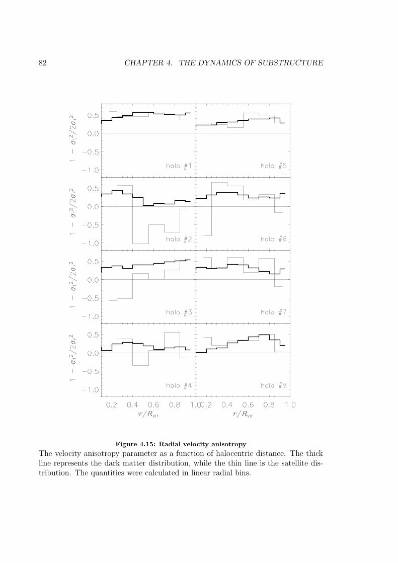
82 CHAPTER 4. THE DYNAMICS OF SUBSTRUCTURE
Figure 4.15: Radial velocity anisotropy
The velocity anisotropy parameter as a function of halocentric distance. The thickline represents the dark matter distribution, while the thin line is the satellite dis-tribution. The quantities were calculated in linear radial bins.

4.5. HOST AND SATELLITE KINEMATICS 83
To further investigate the velocity bias we measure the variation from an isotropic
velocity distribution using the anisotropy parameter, as seen in Figure 4.15
β = 1 − σ2t /2σ2
r , (4.13)
where σt measures the variance in the tangential and σr in radial direction. Once
again, the dark matter (βDM) and satellite distribution (βsat) were averaged in lin-
early spaced radial bins, normalised by the virial radius. The dark matter distri-
bution is represented by the thick histogram and the satellite galaxies by the thin
histogram. For an isotropic distribution β = 0; if β → 1, then the velocities are
preferentially radial; if β → −∞, they are preferentially tangential.
The standard way to represent β is on a logarithm scale starting from the in-
ner percent of the virial radius. Cole & Lacey (1996) and Thomas et al. (1998)
employed this technique and measured a linear increase in βDM, starting with essen-
tially isotropic orbits close to the halo core and becoming increasingly radial in the
outer regions. In keeping with previous figures we plot the data on a linear scale.
This makes it difficult to compare to this work. However, our value for βDM does
follow the same general radial relationship seen in earlier studies.
In general βsat for the substructure population (broadly) follows the dark matter
distribution. However, for halos #2 and #3, satellite orbits are generally more
tangential than the dark matter background.
Finally, to gain further insight into the velocity distributions of the satellite and
dark matter distributions we investigated the radial variation of the radial velocity
component. When normalised by the maximum circular velocity for all eight halos,
we find that the fraction vr,DM/V maxcirc is essentially zero. Although, we do see signs
of a slight dip in the outer regions. This dip is a characteristic signature of in-fall
into the system.
4.5.1 Observational Impact
One way Astronomers determine the mass of galaxy cluster by assuming that the
galaxy distribution is virialised. The virial theorem then gives (Heisler, Tremaine &
Bahcall 1985):
Mvir =Rvirσ
2v
G. (4.14)
84 CHAPTER 4. THE DYNAMICS OF SUBSTRUCTURE
Figure 4.16: Satellite velocity dispersion vs Host halo mass
The velocity dispersion of the satellite galaxies within the virial radius of the hosthalo as a function of host halo mass.
In practice, however, the observational determination of the correct radius Rvir
and velocity dispersion σv are far from straightforward, as it is difficult to determine
whether or not a galaxy is a member of a cluster. Furthermore, even though we have
just learned that the satellites are “stationary”, the existence of the slight global
velocity bias (cf. Table 4.2) does impact the determination of cluster masses. Or in
other words, the observed positive bias will result in an over-estimation of the halo
mass when relying on the dynamics of its substructure.
From our simulations we find (to no surprise) that the velocity dispersion of a
system of galaxies is a reliable indicator of the depth of the potential associated
with the system. Even though we do not have a broad mass range (Mvir ∼ 1 −3 × 10¹⁴h−1 M) to test this hypothesis we reconstruct the expected relationship
between mass Mvir and velocity dispersion σv,sat of the satellite galaxies within the
virial radius of the host halo. The results are presented in Figure 4.16. Each of our
halos scatter about the expected analytical relationship:
σv ∼ M1/3vir (4.15)
4.6. CONCLUSIONS 85
This relationship can easily be understood analytically when we combine Eq. (4.14)
and our definition for virial radius ∆virρb = 3Mvir/(4πR3vir). The solid line displayed
in the figure is the best fit power law to our eight data points. The logarithmic slope
was found to be ∼ 0.329, sufficiently close to the expected value of 1/3 .
4.6 Conclusions
In Chapter 2 we analysed the differences between the host halos. In the first part of
this chapter we described global properties of the satellite populations, such as rich-
ness. Through this analysis we discovered that our sample of dark matter galaxy
clusters sampled a variety of triaxialities, formation times and mass/satellite ac-
cretion rates and formation histories (from quiescent to violent) despite being of
comparable mass. Even though the differences between the host halos we found
considerable similarities between the satellite populations.
These similarities are dramatically demonstrated in the satellites orbital distri-
bution. The average orbital eccentricity of the satellites was found to be e ≈ 0.6
with minimal scatter (σ ≈ 0.2). Moreover, the average pericentre distance of the
satellites was p ∼ 35% of the virial radius for all halos, again with minimal scat-
ter (σ ≈ 0.1). Satellites that were disrupted while orbiting within the host’s virial
radius were replaced with a mass-less tracer particle and hence we were also able
to present their orbital parameters at redshift z = 0. We found that even though
they have smaller eccentricities (ed ≈ 0.34) than the surviving ones, their pericentre
distributions are nearly identical. Since the pericentre distributions of both surviv-
ing and disrupted satellites were similar, implication is that the disrupted satellites
spend more time in the deeper regions of the potential well. As such, they experience
stronger tidal forces for longer periods, and are thus being disrupted more readily.
We also noticed that satellites with more orbits tend to have smaller eccentricities.
Difficult to explain through the application of dynamical friction we attribute this
to the satellite’s response to the growing host halo.
In comparison to the host halo we also found that the satellite populations on
average held approximately 10% of the host’s mass, with the majority of that mass
locked in the larger satellites.
Further, the local velocity bias at all radii is greater than one and this increases
as we move closer to the halo centre. Since this is a characteristic for each of

86 CHAPTER 4. THE DYNAMICS OF SUBSTRUCTURE
our halos, it strengthens the case that this is a general pattern of the satellite
population in dark matter halos. For the global velocity bias we find an average
〈bv,global〉 ∼ 1.103 ± 0.002, a slight, but significant, positive bias. Further, if we
restrict the global velocity bias calculation to satellites that have had at least one
orbit we observe a 7% decrease in bias to 〈bv,global〉 ∼ 1.021 ± 0.002. Thus when
we just consider the “virialised” satellites, the bias nearly vanishes. Finally we
recovered the σv ∼ M1/3 relationship between satellite velocity dispersion and halo
mass.
Surprisingly, all the above stated results appear to be independent of the actual
host halo and its history. We were unable to identify any trends with richness,
triaxiality and/or formation time (other than the number of orbits). Such similarities
are suggestive of potential additional underlying CDM universal laws.
Chapter 5
Anisotropy of Substructure Orbits
“I think it’s one of the scars in our culture that we have
too high an opinion of ourselves. We align ourselves with
the angels instead of the higher primates.”
- Angela Carter
5.1 Introduction
Observations of the distribution of bright elliptical galaxies within the Virgo galaxy
cluster show a remarkable collinear arrangement (West & Blakeslee 2000). Moreover,
this axis also appears to be part of a filamentary bridge connecting Virgo and the
rich cluster Abell 1367. This phenomenon has already been recognized (Arp 1968;
Bingegeli, Tammann & Sandage 1987) but only with accurate measurements of
distance did it become possible to discriminate between this being a genuine three-
dimensional structure or merely a chance alignment of galaxies. West & Blakeslee
(2000) based their distances upon the surface brightness fluctuations method (cf.
Blakeslee, Ajhar & Tonry 1999 for a recent review), concluding that not only were
the brightest cluster members distributed anisotropically over the cluster, but the
distribution of dwarf ellipticals was elongated in the same direction (Bingelli 1999).
Plionis et al. (2003) investigated this substructure-cluster correlation statistically
using 303 Abell clusters. They affirm that there is indeed such a signal and also
that this signal is related to the dynamical state (and the environment) of the cluster.
87

88 CHAPTER 5. ANISOTROPY OF SUBSTRUCTURE ORBITS
Moreover, even on smaller scales – in galactic systems – there are clear obser-
vational indications that the distribution of the orbits of satellite galaxies is biased
towards the galactic pole (Holmberg 1969) giving an anisotropic distribution. Zarit-
sky et al. (1997) found that satellites of (isolated) disk galaxies are scattered asym-
metrically about the parent galaxy and aligned preferentially with the disk minor
axis. At first this signal (dubbed the Holmberg effect) was only prominent for dis-
tances out to ∼50 kpc from the host (Holmberg 1969), but an analysis based on
a much larger sample (cf. Zaritsky et al. 1993) of satellites extends it to 200 kpc
(Zaritsky et al. 1997). This result is confirmed by a study of the satellites or-
biting M31 (Hartwick 2000; Grebel, Kolatt & Brandner 1999). In addition, for
the one galaxy where individual satellite orbits are known, the Milky Way, there
is also evidence that that the orbits are preferentially polar (Zaritsky & Gonzalez
1999). This is derived from information based upon the alignment of satellites on the
sky (Kunkel & Demers 1976; Lynden-Bell 1982), the orientation of the Magellanic
Stream (Mathewson, Clearly & Murray 1974), the three-dimensional distribution
of satellites (Majewski 1994; Hartwick 1996), and their actual velocities (Scholz &
Irwin 1994).
All these observations clearly indicate that on scales spanning from galaxy clus-
ters down to galaxies there is a signal indicating a correlation between the align-
ment of substructure and the shape of the gravitational potential this substructure
moves in. However, the source of this alignment of satellites has been debated
for a number of years, with two potential solutions suggested to explain this puz-
zling arrangement. If the distribution of in-falling satellites is initially spherical,
then dynamical selection may preferentially destroy or suppress the star-formation
in those on more equatorial orbits1. For instance, Penarubbia, Kroupa & Boily
(2002) have argued that in flattened dark matter halos, the timescale for dynam-
ical friction is substantially longer for satellites that are on polar orbits. Alterna-
tively, the present non-isotropic distribution of satellite systems may reflect the fact
that it has always been non-isotropic, with the satellites being accreted along pre-
ferred directions. These hypotheses can be readily tested in numerical simulations
of structure formation. However, in previous attempts to decipher this signal from
cosmological N -body simulations there still remains a certain amount of uncertainty
(Zaritsky et al. 1997).
1With equatorial we mean ”perpendicular to the major axis”
5.2. ORBIAL ALIGNMENT WITH HOST HALO 89
The first fully self-consistent simulations targeting the subject were performed by
Tormen (1997). They though lacked resolution in time, space and mass to perform
a detailed analysis of the satellite population for differing environments, and hence
more refined simulations are required. Tormen (1997) could not follow the satellite
distribution within the host’s virial radius but rather tracked all progenitors prior
to accretion. This allowed him to analyse the in-fall pattern rather than the orbital
evolution of the satellites.
In this chapter we investigate the anisotropy of satellite orbits within our sim-
ulations. The brief outline of the chapter is as follows. We first discuss the orbital
alignment with host halo axis in Section 5.2. Following that we investigate the
connection between the large-scale structure and our sub-halo populations in Sec-
tion 5.3. We then hypothesise a solution to the Holmberg effect in Section 5.4 and
make our concluding remarks in the final Section 5.5.
5.2 Orbial alignment with host halo
Figure 5.1 presents the (normalized) distribution of angles between ~Raposat and ~E1,host.
~E1,hostis derived by the triaxiality of the host system (cf. Section 2.4.2). This graph
shows that there is a clear trend in at least six of the eight halos for the two vectors
to be aligned (the distribution peaks at 0 and 180, respectively) meaning that the
orbits of the satellites are preferentially found along the major axis of the host.
Figure 5.2 shows the (normalized) distribution of angles between the angular
momentum vector ~Laposat =~Rapo
sat ×~V aposat of the satellite at its last apocenter and ~E1,host,
clearly revealing evidence for these two vectors to be parallel (distribution peaks
at 90). We like to stress that only satellite galaxies that at least had one or more
complete orbits were taken into account in Figure 5.1 and Figure 5.2; the figure is not
based upon the in-fall pattern of satellites as investigated by, for instance, Tormen
(1997). We also need to stress that the distributions presented in that Figure are
normalized, i.e. they are corrected for the bias introduced by plotting them as a
function of the angle θ rather than cos θ. The data is binned equally spaced in angle
ranging from 0 to 180, and therefore the area probed on the sphere varies with
θ. Further, the distribution needed to be normalized by the the respective area A
specified by the actual range of angles [θ−∆θ/2, θ+∆θ/2]. This area is proportional
to A ∝ cos(θ − ∆θ/2) − cos(θ + ∆θ/2).
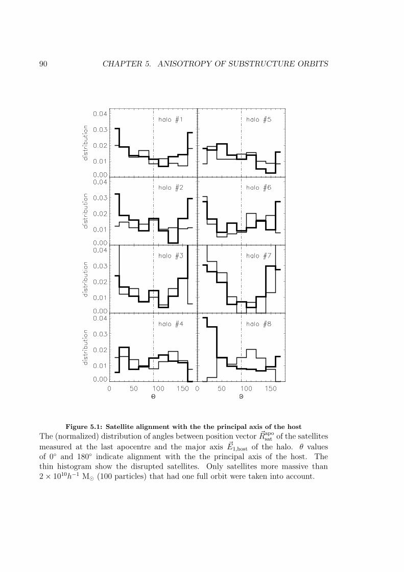
90 CHAPTER 5. ANISOTROPY OF SUBSTRUCTURE ORBITS
Figure 5.1: Satellite alignment with the the principal axis of the host
The (normalized) distribution of angles between position vector ~Raposat of the satellites
measured at the last apocentre and the major axis ~E1,host of the halo. θ valuesof 0 and 180 indicate alignment with the the principal axis of the host. Thethin histogram show the disrupted satellites. Only satellites more massive than2 × 1010h−1 M (100 particles) that had one full orbit were taken into account.
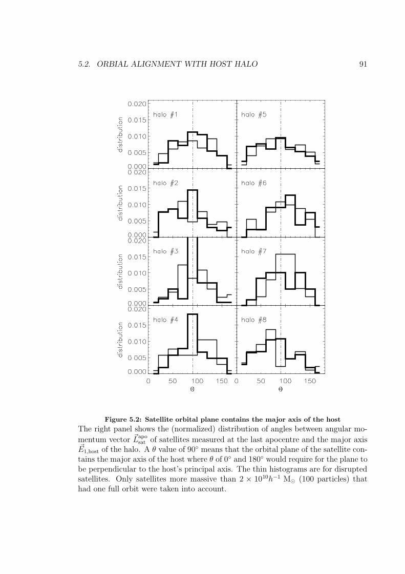
5.2. ORBIAL ALIGNMENT WITH HOST HALO 91
Figure 5.2: Satellite orbital plane contains the major axis of the host
The right panel shows the (normalized) distribution of angles between angular mo-
mentum vector ~Laposat of satellites measured at the last apocentre and the major axis
~E1,host of the halo. A θ value of 90 means that the orbital plane of the satellite con-tains the major axis of the host where θ of 0 and 180 would require for the plane tobe perpendicular to the host’s principal axis. The thin histograms are for disruptedsatellites. Only satellites more massive than 2 × 10¹⁰h−1 M (100 particles) thathad one full orbit were taken into account.

92 CHAPTER 5. ANISOTROPY OF SUBSTRUCTURE ORBITS
As outlined in the introduction to this Chapter there are two possible scenar-
ios that explain the substructure-cluster alignment found in observations of galaxy
clusters (Plionis et al. 2003; West & Blakeslee 2000) and the analysis of N -body-
simulations presented in this study. Either some dynamical process can be held
responsible, meaning that initially the orbits were randomly distributed and only
some satellites survive to give rise to the observed correlation in Figure 5.1 and
Figure 5.2, or alternatively, their orbital parameters are imprinted upon them at
the time they enter the host halo as already pointed out by Tormen (1997).
“Dynamical destruction”, whereby satellites on more equatorial orbits suffer
more tidal disruption, can be rejected because a comparable (although not as pro-
nounced) alignment signal is found when restricting the analysis to those satellites
that are in fact disrupted: We placed mass-less tracer particles at the last centre
of the satellites before they were classified ”disrupted”. These “disrupted systems”
are presented as the thin lines in Figure 5.1 and Figure 5.2.
We therefore conclude that it must be the initial distribution of the satellite
systems that is responsible for the present day alignment. For example, galaxies are
”funnelling along the filaments” (Kitzbichler & Saurer 2003) which has also been
confirmed by X-ray observations of the spatial distribution of substructure in galaxy
clusters (West, Jones & Forman 1995) and biases the types of possible orbits.
5.3 Alignment with large-scale structure
It would now be reassuring to confirm a link between the host halo shape and the
surrounding environment, i.e. are the filaments that feed the halo with material pref-
erentially angled with respect to the orientation of the host halo? When projecting
the positions of the satellites onto a sphere at the time they enter the virial radius of
the host it is clear that they are not randomly distributed; they cluster in directions
linked to the filamentary structure surrounding the host halo, as found before ob-
servationally (e.g. West & Blakeslee 2003; Plionis & Basilikos 2002, and references
therein) and in N -body-simulations (e.g. Faltenbacher 2002; Hatton & Ninin 2001;
Onuora & Thomas 2000; Colberg et al. 1999; Splinter et al. 1997; Tormen 1997).
Tormen (1997) already pointed out that there is a strong alignment between the
distribution of in-falling satellite galaxies and the shape of the dark matter host.
However, Tormen’s simulations did not have the spatial and mass resolution to in-

5.4. HOLMBERG EFFECT 93
vestigate the orbits of satellites within the host halo. We are, for the first time,
tracing the dynamics of the satellites within the dark matter hosts confirming that
the alignment for both, disrupted and surviving, satellites is maintained for several
orbital periods. Figure 5.3 now presents a visual impression of the trajectories of all
surviving satellites identified at formation time of host halo #3 until redshift z = 0,
qualitatively supporting the scenario that these orbits are linked to the filamentary
structure which will leave its imprint in observed anisotropy.
Plionis et al. (2003) also established a link between the alignment and the dy-
namical age of the clusters. Our simulations though show that this finding can not
be generalized: both our oldest halos, in which the satellites had as many as 4–5
orbits, do show the correlation signal. We do not observe a trend for a ”randomi-
sation” of the orbits in older halos. The satellites actually preserve the alignment
with the host they had when they first fell into the cluster.
5.4 Holmberg effect
In Section 5.1 we showed that the (observational) substructure-alignment signal
spans from galaxy clusters down to galactic scales. Our results are mostly applicable
to the former, and any extrapolation to smaller scales has to be handled with care.
In the case for galaxies, for instance, the interaction between the galactic disk and
the incoming satellite could enhance destruction in the galaxy plane, i.e. satellite
on prograde orbits decay faster than the ones on retrograde (or polar) orbits due
to orbital resonances between the disk and the satellites (Penarubbia, Kroupa &
Boily 2002). Based on theoretical and numerical studies (cf. Lacey & Cole 1993 and
Moore et al. 1999) it should be possible to re-scale our simulations to a Milky Way
sized object by requiring that the maximum of the circular velocity curves of our
halos equals 220 km s−1. The scaling factor lies in the range of about 4–5 (cf. vmaxcirc
values in Table 2.5) and hence our “rescaled dark matter halos” would correspond
to the ones in the observational data with virial radii in the range 260–295h−1 kpc.
This scaling factor in length entails a scaling in mass of 64–125 (simply the length
scale to the power of three). This brings the mass of our galaxy clusters down to
∼ 1012h−1 M which agrees with the dark matter mass inferred for our Milky Way
(Freeman 1996). More problematic, however, are the ages of our systems: our halos
are only ≤8.3 Gyrs old opposed to 12 Gyrs for the Milky Way. Satellites in the
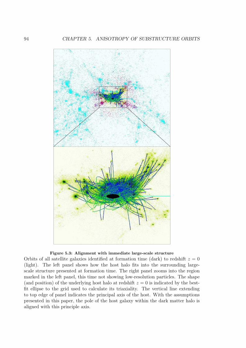
94 CHAPTER 5. ANISOTROPY OF SUBSTRUCTURE ORBITS
Figure 5.3: Alignment with immediate large-scale structure
Orbits of all satellite galaxies identified at formation time (dark) to redshift z = 0(light). The left panel shows how the host halo fits into the surrounding large-scale structure presented at formation time. The right panel zooms into the regionmarked in the left panel, this time not showing low-resolution particles. The shape(and position) of the underlying host halo at redshift z = 0 is indicated by the best-fit ellipse to the grid used to calculate its triaxiality. The vertical line extendingto top edge of panel indicates the principal axis of the host. With the assumptionspresented in this paper, the pole of the host galaxy within the dark matter halo isaligned with this principle axis.
5.5. CONCLUSION 95
Milky Way had the chance to complete nearly twice as many orbits leaving more
space for an explanation based upon the dynamical destruction scenario.
When re-scaling our data, putting aside the age issue, and trying to explain the
Holmberg effect, another uncertainty comes into play: the orientation of the stellar
disk. In a triaxial potential there are in general stable closed orbits about both the
major and the minor axis (e.g., Binney & Tremaine 1987). So, in principal the disk
plane could either be perpendicular to the major or perpendicular to the minor axis.
Under the assumption it lies perpendicular to the major axis of the dark matter halo
the satellites in our simulations will be on polar orbits. There are indications that
this configuration results in the most stable disk configuration within a triaxial halo
(Hayashi et al. 2003). Moreover, even though there are clear indications that the
angular momentum of the dark matter is well aligned with the minor axis of the
halo (e.g. Warren et al. 1992), van den Bosch et al. (2002) showed that the angular
momentum of the baryonic component (i.e. gas) not necessarily follows that of the
dark matter distribution. They found an average misalignment between ~Lgas and~LDM of the order of 40 in their numerical simulations. Hence the orientation of the
galactic disk with respects to the dark matter halo is not well determined. Turning
to observations does not resolve this question, with studies of polar rings indicating
strongly oblate halos (i.e. Iodice et al. 2003), while others suggest dark matter halos
are more spherical, or even oblate (Olling & Merrifield 2000; Ibata et al. 2001). The
situation is not at all clear, but the assumption that disks are perpendicular to the
major axis (which is in agreement with results presented by Hayashi et al. 2003)
would provide an explanation for the Holmberg effect, even though this is a very
speculative interpretation.
5.5 Conclusion
In conclusion this chapter presented an analysis of our cosmological simulations that
focused on the relationship between the orbits of satellite galaxies and their host
halos. We show that the apocentres of the orbits of these satellites are preferentially
found within a cone of opening angle ∼40 around the major axis of the host halo, in
accordance with the observed anisotropy found in galaxy clusters. We do, however,
note that a link to the dynamical age of the cluster is not well established as both
our oldest dark matter halos do show a clear anisotropy signal. Further analysis

96 CHAPTER 5. ANISOTROPY OF SUBSTRUCTURE ORBITS
connects this distribution to the in-fall pattern of satellites along the filaments.
Thus we therefore conclude that the satellite orbits are determined by their initial
distribution i.e. the large-scale structure rather than some ”dynamical selection”
during their life within the host’s virial radius.
Since the publication of this chapter as a paper there has been an ongoing dis-
cussion in the literature.
Lee & Kang (2005) applied similar ideas to develop an algorithm for reconstruct-
ing the triaxial shapes of dark matter halos from the anisotropic spatial distributions
of sub-halos.
Zentner et al. (2005) extended our work from clusters to galaxies and found
the same results on galactic scales, which smaller and more dynamically evolved
systems.
Zentner’s result strengthens our explanation of the origins of the Holmberg effect.
However, Balin et al. 2005 showed that the galactic disks do not align with the major
axis of the dark halo, which would make this interpretation of the Holmberg effect
contradictory.
This is emphasised by additional recent observational results. Sales & Lambas
(2004) analysed the 2dF Galaxy Redshift Survey finding strong statistical evidence of
the Holmberg effect. However, Brainerd (2004) analysed the distribution of satellite
galaxies relative to isolated host galaxies in the Sloan Digital Sky Survey (SDSS)
finding significant anisotropy with satellites aligning with the major axes of the hosts
thus in stark contrast to the Holmberg effect and in favour with our results.
There obviously needs to be more research to be done to finally resolve the
mystery of the Holmberg effect.

Chapter 6
Outskirts of Dark Matter halos
“When you talk with me about my research, do not ask
me what I found; I found nothing. Ask me what I invented,
what I made up from and out of my data.”
- Sandelowski (1994)
6.1 Introduction
The relationship between galaxy morphology and local environment (i.e. the morphology-
density relation) was first noticed by Hubble & Humason (1931), where they reported
that field and cluster galaxy populations differ. Oemler (1974) extended this finding
by showing that the relationship held for differing clusters richness. The field truly
emerged when Dressler (1980) demonstrated the strong relationship over five orders
of magnitude between the local density of galaxies and the proportions of different
morphological types. Bhavsar (1981), de Souza et al. (1982), and Postman & Geller
(1984) extended this work further to include the environments of both loose and
compact groups. Recently, Aguerri et al. (2004) performed a thorough analysis of
116 bright galaxies in the Coma cluster, finding that bluer objects are located at
larger projected radii while simultaneously showing a larger velocity dispersion than
their red counterparts. Moreover, the bluest objects also host the most prominent
disks contrary to systems observed close to the cluster centre or in high-density en-
vironments. Environmental dependence of galactic stellar populations is also seen
in the Butcher-Oemler effect (Butcher & Oemler 1978, Kodama & Bower 2001) with
97
98 CHAPTER 6. OUTSKIRTS OF DARK MATTER HALOS
clusters at higher redshifts showing a greater fraction of blue objects than are seen
at present.
The above observational work supports the idea that galaxies in clusters are
substantially different from galaxies in the field. But the origins of these morphology-
density relationships are still not fully understood with several large and small scale
mechanisms proposed to explain their existence, including ram pressure stripping
(Gun & Gott 1972), tidal stripping/star formation (Merritt 1983, 1984), starvation
(Larson, Tinsley & Caldwell 1980), galaxy merger and harassment (Icke 1985; Moore
et al. 1996) and dynamics (Tsuchiya & Shimada 2000).
Recent cosmological simulations (both hydrodynamical and N -body) have pro-
vided valuable insight into the mechanisms responsible for the morphology-density
relationship (Springel et al. 2001; Goto et al. 2003; Okamoto & Nagashima 2003).
In the analysis which follows, we focus on the dynamics of satellite galaxies as de-
scribed in Chapter 2. But now we concentrate on the outskirts of these clusters, i.e.
distances in the range [Rvir, 2.5Rvir], which (observationally) have only recently been
probed through wide-field optical imaging and spectroscopy (Miyazaki et al. 2002;
Lewis et al. 2002). We will demonstrate that a rich population of galaxies exist
beyond the virial radius most of which have previously spent time near the cluster
centre. We characterise the spatial, velocity and mass properties of this population
and contrast these with those of the spatially coincident newly in-falling galaxies.
Our work complements the earlier studies of Balogh et al. (2000) and Mamon
et al. (2004). Balogh et al. investigated the particle “backsplash” from cosmological
simulations and found that 50 ± 20% of the particles within [R200, 2R200] had passed
through the R200 radius. Mamon et al. recently extended this work to calculate the
maximum backsplash distance for particles to be 2.5R100 and for galaxies 1.7R100.
For later reference and comparison to previous studies by Balogh et al. (2000)
and Mamon et al. (2004) we relate Rvir to other definitions of the virial radius,
namely R200 and R100. According to the NFW profile (Navarro, Frenck & White
1997) the dark matter density in the outer regions of halos drops like ρ ∝ r−3 and
hence Rvir ∼ 1.4R200 and Rvir ∼ R100.
The outline of this chapter is as follows. We investigate the number distribu-
tion of galaxies in the cluster outskirts in Section 6.2, with the mass distribution
discussed in Section 6.3 and the velocity distribution of the satellites investigated in
Section 6.4. We finish with our summary and conclusions in Section 6.5.
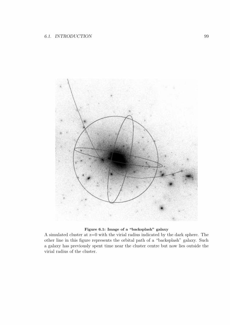
6.1. INTRODUCTION 99
Figure 6.1: Image of a “backsplash” galaxy
A simulated cluster at z=0 with the virial radius indicated by the dark sphere. Theother line in this figure represents the orbital path of a “backsplash” galaxy. Sucha galaxy has previously spent time near the cluster centre but now lies outside thevirial radius of the cluster.
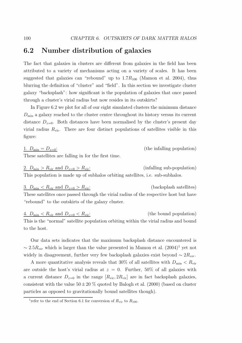
100 CHAPTER 6. OUTSKIRTS OF DARK MATTER HALOS
6.2 Number distribution of galaxies
The fact that galaxies in clusters are different from galaxies in the field has been
attributed to a variety of mechanisms acting on a variety of scales. It has been
suggested that galaxies can “rebound” up to 1.7R100 (Mamon et al. 2004), thus
blurring the definition of “cluster” and “field”. In this section we investigate cluster
galaxy “backsplash”: how significant is the population of galaxies that once passed
through a cluster’s virial radius but now resides in its outskirts?
In Figure 6.2 we plot for all of our eight simulated clusters the minimum distance
Dmin a galaxy reached to the cluster centre throughout its history versus its current
distance Dz=0. Both distances have been normalised by the cluster’s present day
virial radius Rvir. There are four distinct populations of satellites visible in this
figure:
1. Dmin = Dz=0: (the infalling population)
These satellites are falling in for the first time.
2. Dmin > Rvir and Dz=0 > Rvir: (infalling sub-population)
This population is made up of subhalos orbiting satellites, i.e. sub-subhalos.
3. Dmin < Rvir and Dz=0 > Rvir: (backsplash satellites)
These satellites once passed through the virial radius of the respective host but have
“rebound” to the outskirts of the galaxy cluster.
4. Dmin < Rvir and Dz=0 < Rvir: (the bound population)
This is the “normal” satellite population orbiting within the virial radius and bound
to the host.
Our data sets indicates that the maximum backsplash distance encountered is
∼ 2.5Rvir which is larger than the value presented in Mamon et al. (2004)1 yet not
widely in disagreement, further very few backsplash galaxies exist beyond ∼ 2Rvir.
A more quantitative analysis reveals that 30% of all satellites with Dmin < Rvir
are outside the host’s virial radius at z = 0. Further, 50% of all galaxies with
a current distance Dz=0 in the range [Rvir, 2Rvir] are in fact backsplash galaxies,
consistent with the value 50±20 % quoted by Balogh et al. (2000) (based on cluster
particles as opposed to gravitationally bound satellites though).
1refer to the end of Section 6.1 for conversion of Rvir to R100.
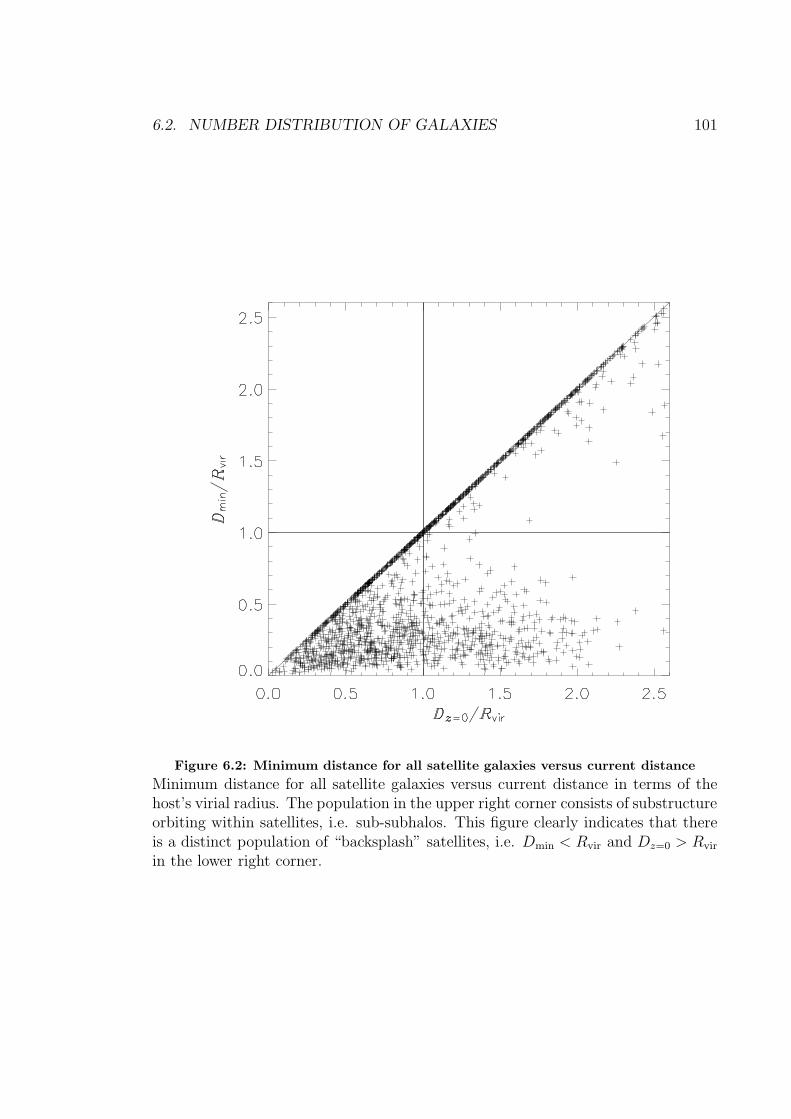
6.2. NUMBER DISTRIBUTION OF GALAXIES 101
Figure 6.2: Minimum distance for all satellite galaxies versus current distance
Minimum distance for all satellite galaxies versus current distance in terms of thehost’s virial radius. The population in the upper right corner consists of substructureorbiting within satellites, i.e. sub-subhalos. This figure clearly indicates that thereis a distinct population of “backsplash” satellites, i.e. Dmin < Rvir and Dz=0 > Rvir
in the lower right corner.
102 CHAPTER 6. OUTSKIRTS OF DARK MATTER HALOS
Figure 6.3: Normalised distribution function of galaxy minimum distance
The relative normalised distribution function of the minimum distance Dmin/Rvir
for the whole galaxy population (thick histograms) and the satellites with currentpositions greater than the virial radius (thin histograms). We note that they bothpeak near 25% of the cluster virial radius.
6.3. MASS DISTRIBUTION OF THE GALAXIES 103
Only 2% of the backsplash population has had more than one orbit (i.e. eight
satellites in total) and most stem from single passages through the host’s virial
radius, respectively. And each of these eight “multiple passage” backsplash galaxies
are found in the range [Rvir, 1.2Rvir] which is close to the host.
We now investigate the depth to which backsplash galaxies penetrate the cluster
potential. To this extent we plot in Figure 6.3 the normalised number distribution of
the minimum distance Dmin for the entire satellite population (thick histogram) and
the restricted set of satellites currently outside the virial radius (thin histograms).
It is interesting to note that the distributions are fairly similar for Dmin < Rvir,
i.e. they both peak near 0.25. We stress that this is the minimum distance as
measured over the lifetime of the host halo and hence is not to be confused with
the last pericentre whose distribution peaks at about 35% of Rvir (cf. Chapter 4).
Figure 6.3 reveals that the a number of the galaxies that are now in the outskirts
of the cluster have had passages as close to the host as their bound counterparts
which implies that the former are on highly radial orbits. This is consistent with
the findings of Solanes et al. (2001) who found evidence that gas-poor spirals in HI
deficient clusters move in orbits more radial than those of the gas-rich objects. In
fact, 90% of our backsplash satellites once passed within the inner 50% of the virial
radius.
In summary the number of backsplash galaxies is significant and should be ac-
counted for when interpreting the galaxy morphology-density relationship. These
galaxies penetrate deep within the cluster potential, as deep as their bound coun-
terparts. Hence, they should be sampling the large and small-scale transformation
mechanisms alluded to in the introduction. For example, if we used the prescriptions
outlined in Treu et al. (2003), these galaxies would also have undergone starvation,
ram pressure stripping, tidally triggered star formation and significant tidal strip-
ping, thus confusing any correlation of the galaxy’s morphology with local environ-
ment.
6.3 Mass distribution of the galaxies
One way to gauge the significance of these transformation mechanisms is to investi-
gate the mass loss of a galaxy during its encounter with the cluster. To this extent
we focus only on the backsplash population and plot the relative mass lost over the
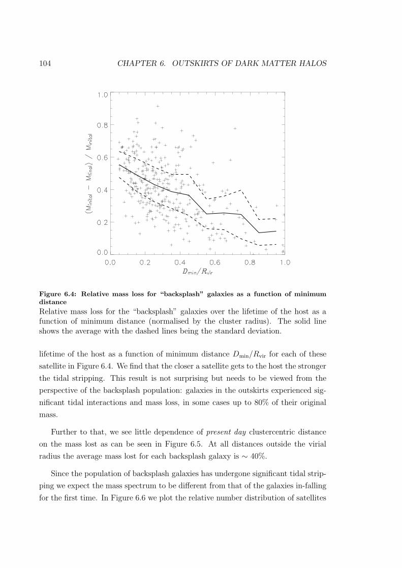
104 CHAPTER 6. OUTSKIRTS OF DARK MATTER HALOS
Figure 6.4: Relative mass loss for “backsplash” galaxies as a function of minimumdistance
Relative mass loss for the “backsplash” galaxies over the lifetime of the host as afunction of minimum distance (normalised by the cluster radius). The solid lineshows the average with the dashed lines being the standard deviation.
lifetime of the host as a function of minimum distance Dmin/Rvir for each of these
satellite in Figure 6.4. We find that the closer a satellite gets to the host the stronger
the tidal stripping. This result is not surprising but needs to be viewed from the
perspective of the backsplash population: galaxies in the outskirts experienced sig-
nificant tidal interactions and mass loss, in some cases up to 80% of their original
mass.
Further to that, we see little dependence of present day clustercentric distance
on the mass lost as can be seen in Figure 6.5. At all distances outside the virial
radius the average mass lost for each backsplash galaxy is ∼ 40%.
Since the population of backsplash galaxies has undergone significant tidal strip-
ping we expect the mass spectrum to be different from that of the galaxies in-falling
for the first time. In Figure 6.6 we plot the relative number distribution of satellites

6.3. MASS DISTRIBUTION OF THE GALAXIES 105
Figure 6.5: Relative mass loss for “backsplash” galaxies as a function of currentposition
Relative mass loss for the “backsplash” galaxies over the lifetime of the host as afunction of current position (normalised by the cluster radius). The solid line showsthe average with the dashed lines being the standard deviation.
106 CHAPTER 6. OUTSKIRTS OF DARK MATTER HALOS
with a certain mass Msat measured in terms of the host’s virial mass Mhost. The
thin histogram represents the backsplash population and the thick histogram shows
the in-falling population. To better discriminate between these two populations we
fitted the mass spectra to a simple power-law
n(M) = CMα (6.1)
There is a marginal difference between the slopes, the backsplash population having
α = 0.9 ± 0.3 whereas the in-falling satellites distribution is characterised by α =
0.7 ± 0.3. The steeper slope of the backsplashed galaxies reflects the lack of larger
satellites and an over-abundance of smaller galaxies, respectively. This tilt in the
mass spectrum is readily explained by the mass loss highlighted in Figure 6.4. We
note that the first mass bin was not used in fitting the power-law as it simply reflects
the absolute mass cut of 2 × 10¹⁰ h−1 M (i.e. we did not use a relative mass cut
with respect to the mass of the host).
6.4 Velocity properties of backsplash galaxies
To populate the outskirts of clusters, galaxies that once passed through the virial
radius and close to the centre of the host must have had high velocities. In this
section we explore the relative velocities of satellite galaxies within the cluster and
its outskirts.
6.4.1 A kinematically distinct backsplash population
Figure 6.7 shows the absolute value of the relative velocity between a satellite galaxy
and the host cluster as a function of current clustercentric distance. We present the
results for two populations again, namely the in-falling satellites that are still outside
the virial radius (diamonds) and the backsplash galaxies alongside galaxies within
the virial radius (crosses).
At the virial radius the maximum relative velocity for a galaxy in our data set is
1500 km s−1 with no galaxy farther away having a greater velocity. This finding can
be used to explore the two competing models for the ram-pressure stripping observed
in NGC 4522, a spiral galaxy in the Virgo cluster with a distance close to the virial
radius (Vollmer et al. 2001). Kenney et al. (2004) suggested two possible scenarios to
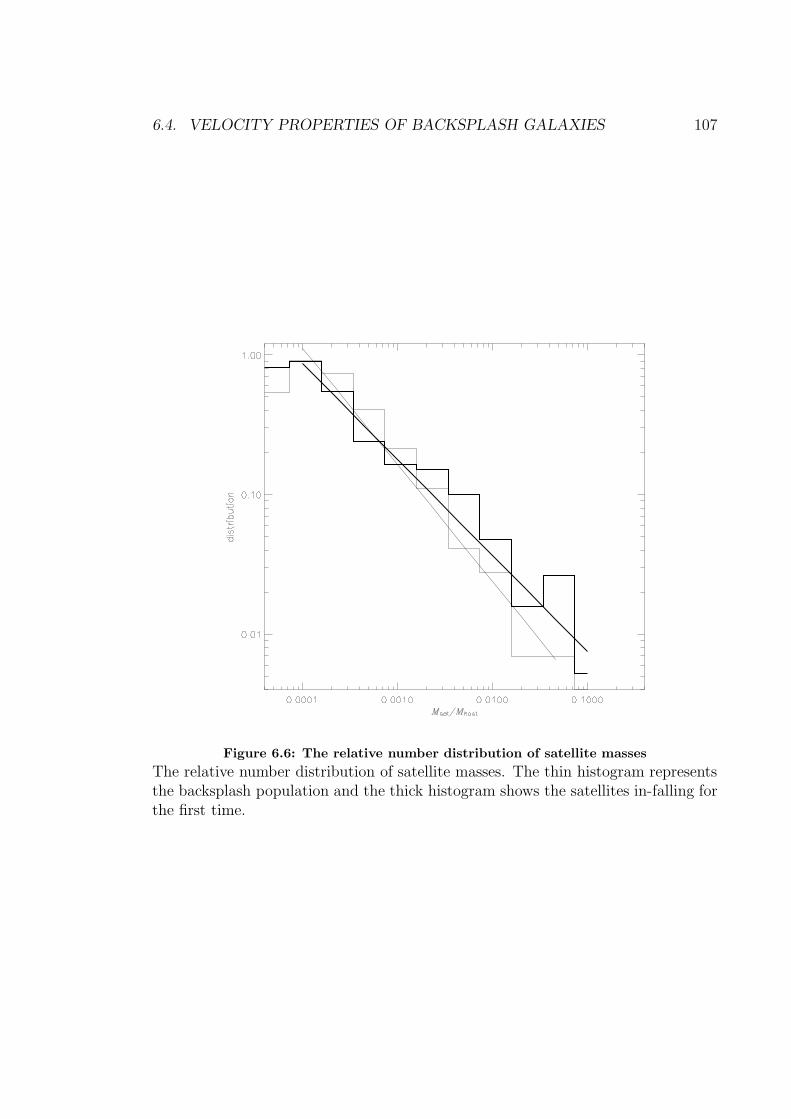
6.4. VELOCITY PROPERTIES OF BACKSPLASH GALAXIES 107
Figure 6.6: The relative number distribution of satellite masses
The relative number distribution of satellite masses. The thin histogram representsthe backsplash population and the thick histogram shows the satellites in-falling forthe first time.

108 CHAPTER 6. OUTSKIRTS OF DARK MATTER HALOS
Figure 6.7: Absolute relative velocity for the in-falling satellites
The absolute value of the relative velocity for the in-falling satellites (diamonds) andthe population of satellite that have crossed the virial radius at sometime (crosses) asa function of current cluster distance to the host. The middle solid lines representaverages with the outer lines being the standard deviations. Note the kinematicdistinction between the populations.
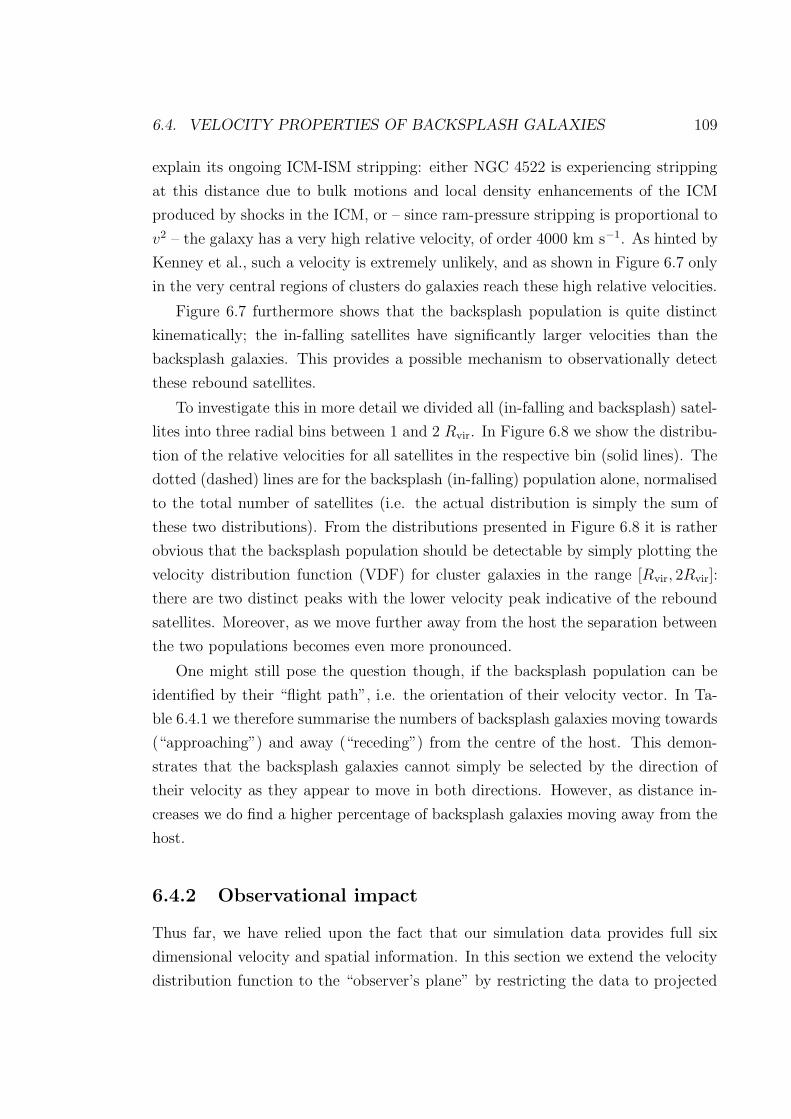
6.4. VELOCITY PROPERTIES OF BACKSPLASH GALAXIES 109
explain its ongoing ICM-ISM stripping: either NGC 4522 is experiencing stripping
at this distance due to bulk motions and local density enhancements of the ICM
produced by shocks in the ICM, or – since ram-pressure stripping is proportional to
v2 – the galaxy has a very high relative velocity, of order 4000 km s−1. As hinted by
Kenney et al., such a velocity is extremely unlikely, and as shown in Figure 6.7 only
in the very central regions of clusters do galaxies reach these high relative velocities.
Figure 6.7 furthermore shows that the backsplash population is quite distinct
kinematically; the in-falling satellites have significantly larger velocities than the
backsplash galaxies. This provides a possible mechanism to observationally detect
these rebound satellites.
To investigate this in more detail we divided all (in-falling and backsplash) satel-
lites into three radial bins between 1 and 2 Rvir. In Figure 6.8 we show the distribu-
tion of the relative velocities for all satellites in the respective bin (solid lines). The
dotted (dashed) lines are for the backsplash (in-falling) population alone, normalised
to the total number of satellites (i.e. the actual distribution is simply the sum of
these two distributions). From the distributions presented in Figure 6.8 it is rather
obvious that the backsplash population should be detectable by simply plotting the
velocity distribution function (VDF) for cluster galaxies in the range [Rvir, 2Rvir]:
there are two distinct peaks with the lower velocity peak indicative of the rebound
satellites. Moreover, as we move further away from the host the separation between
the two populations becomes even more pronounced.
One might still pose the question though, if the backsplash population can be
identified by their “flight path”, i.e. the orientation of their velocity vector. In Ta-
ble 6.4.1 we therefore summarise the numbers of backsplash galaxies moving towards
(“approaching”) and away (“receding”) from the centre of the host. This demon-
strates that the backsplash galaxies cannot simply be selected by the direction of
their velocity as they appear to move in both directions. However, as distance in-
creases we do find a higher percentage of backsplash galaxies moving away from the
host.
6.4.2 Observational impact
Thus far, we have relied upon the fact that our simulation data provides full six
dimensional velocity and spatial information. In this section we extend the velocity
distribution function to the “observer’s plane” by restricting the data to projected
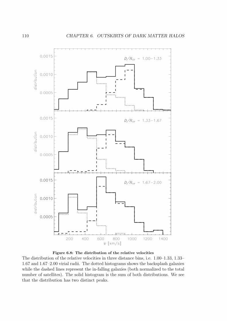
110 CHAPTER 6. OUTSKIRTS OF DARK MATTER HALOS
Figure 6.8: The distribution of the relative velocities
The distribution of the relative velocities in three distance bins, i.e. 1.00–1.33, 1.33–1.67 and 1.67–2.00 virial radii. The dotted histograms shows the backsplash galaxieswhile the dashed lines represent the in-falling galaxies (both normalized to the totalnumber of satellites). The solid histogram is the sum of both distributions. We seethat the distribution has two distinct peaks.
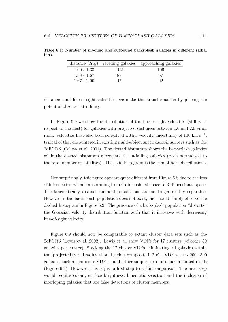
6.4. VELOCITY PROPERTIES OF BACKSPLASH GALAXIES 111
Table 6.1: Number of inbound and outbound backsplash galaxies in different radialbins.
distance (Rvir) receding galaxies approaching galaxies
1.00 - 1.33 102 1061.33 - 1.67 87 571.67 - 2.00 47 22
distances and line-of-sight velocities; we make this transformation by placing the
potential observer at infinity.
In Figure 6.9 we show the distribution of the line-of-sight velocities (still with
respect to the host) for galaxies with projected distances between 1.0 and 2.0 virial
radii. Velocities have also been convolved with a velocity uncertainty of 100 km s−1,
typical of that encountered in existing multi-object spectroscopic surveys such as the
2dFGRS (Colless et al. 2001). The dotted histogram shows the backsplash galaxies
while the dashed histogram represents the in-falling galaxies (both normalised to
the total number of satellites). The solid histogram is the sum of both distributions.
Not surprisingly, this figure appears quite different from Figure 6.8 due to the loss
of information when transforming from 6-dimensional space to 3-dimensional space.
The kinematically distinct bimodal populations are no longer readily separable.
However, if the backsplash population does not exist, one should simply observe the
dashed histogram in Figure 6.9. The presence of a backsplash population “distorts”
the Gaussian velocity distribution function such that it increases with decreasing
line-of-sight velocity.
Figure 6.9 should now be comparable to extant cluster data sets such as the
2dFGRS (Lewis et al. 2002). Lewis et al. show VDFs for 17 clusters (of order 50
galaxies per cluster). Stacking the 17 cluster VDFs, eliminating all galaxies within
the (projected) virial radius, should yield a composite 1–2 Rvir VDF with ∼ 200−300
galaxies; such a composite VDF should either support or refute our predicted result
(Figure 6.9). However, this is just a first step to a fair comparison. The next step
would require colour, surface brightness, kinematic selection and the inclusion of
interloping galaxies that are false detections of cluster members.
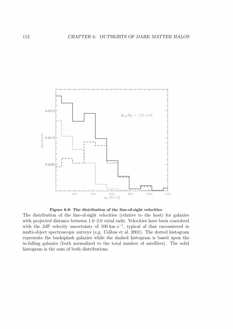
112 CHAPTER 6. OUTSKIRTS OF DARK MATTER HALOS
Figure 6.9: The distribution of the line-of-sight velocities
The distribution of the line-of-sight velocities (relative to the host) for galaxieswith projected distance between 1.0–2.0 virial radii. Velocities have been convolvedwith the 2dF velocity uncertainty of 100 km s−1, typical of that encountered inmulti-object spectroscopic surveys (e.g. Colless et al. 2001). The dotted histogramrepresents the backsplash galaxies while the dashed histogram is based upon thein-falling galaxies (both normalized to the total number of satellites). The solidhistogram is the sum of both distributions.

6.5. CONCLUSIONS 113
6.5 Conclusions
Observational data supports the idea that galaxies in clusters are substantially dif-
ferent from galaxies in the field. There is a clear correlation between galaxy mor-
phology and density of the local environment. However, the origin of this relation
is far from being understood.
In this study we have presented an analysis of satellite galaxies that once passed
through the virial radius close to the centre of their respective host halo, but are
now found outside the virial radius in the outskirts of the cluster. We have shown
that this backsplash population is not negligible and needs to be accounted for
when interpreting the various galaxy morphology relationships and decoupling the
degeneracy between nature and nurture.
We must also appreciate that the in-falling population is not expected to be
pristine. Rather, we would expect that in-fall galaxies have undergone some sort
of pre-processing in groups before entering the cluster too as indicated by the sub-
subhalos in Figure 6.2.
Our results can be summarized as follows:
• 30% of all galaxies that ever came closer to the host than its virial radius are
now located in the range [Rvir,2.5Rvir],
• 50% of all galaxies in the region [Rvir,2Rvir] are backsplash galaxies,
• 90% of the backsplash galaxies penetrated deeper than 50% of Rvir into the
host’s potential,
• during their passage through the cluster, on average the backsplash galaxies
lose 40% of their mass, thus
• the mass spectrum of the backsplash population has a steeper power-law slope
than their in-falling counterparts, thus it has fewer massive galaxies and more
light ones,
• the velocities of the in-falling satellites is too small to account for ram-pressure
stripping in the cluster outskirts,
• the backsplash population has a factor of two smaller relative velocity than
the in-falling satellites, making it kinematically distinct.
114 CHAPTER 6. OUTSKIRTS OF DARK MATTER HALOS
When transforming the last result into the observers plane though, the velocity
separation between the in-falling and backsplash population is removed. However,
the backsplash population should still be detectable as it is responsible for a contin-
uous rise in the distribution function towards low line-of-sight velocities.
Our results suggest that we not only expect the backsplash population to ex-
perience various large-scale transformation mechanisms, but also small-scale ones,
undergoing starvation, ram pressure stripping, tidally triggered star formation and
significant tidal stripping.
Chapter 7
Mapping Substructure debri
“I have an existential map. It has You are here written
all over it.”
- Steven Wright
7.1 Introduction
With the discovery of stellar streams within the Milky Way (Helmi et al. 1999;
Chiba & Beers 2000; Ibata et al. 2001c & 2002; Brook et al. 2003; Yanny et al. 2003;
Navarro, Helmi & Freeman 2004; Majewski et al. 2004) and M31 (Ibata et al. 2001a;
McConnachie et al. 2004) and streams and shells in clusters ( Trentham & Mobasher
1998; Gregg & West 1998; Calcaneo-Roldan 2000; Feldmeier et al. 2002) they have
become a standard fixture in our understanding of galaxy and cluster formation.
These streams provide important observational support for the hierarchical build-up
of galaxies and clusters and the Λ-dominated cold dark matter (ΛCDM) paradigm.
Future observational experiments such as RAVE 1 and GAIA2 are designed to shed
further light on the importance of streams in galaxy formation. Thus to better
interpret this observational data coming online in the near future it is necessary to
have clear theoretical understanding of the stellar streams left behind by dissolving
satellites (sub-halos).
The most common approach to this has been to simulate the disruption of indi-
vidual satellite galaxies in static analytical potentials representative of the distribu-
1http://astronomy.swin.edu.au/RAVE/2http://astro.estec.esa.nl/GAIA/
115

116 CHAPTER 7. MAPPING SUBSTRUCTURE DEBRI
tion of dark matter (DM) halos (Kojima & Noguchi 1997; Helmi & de Zeeuw 2000;
Harding et al. 2001; Ibata et al. 2002; Bekki et al. 2003; Majewski et al. 2004).
Such simulations have provided great insight into the formation of stellar (Ibata
et al. 2002) and gaseous (Yoshizawa & Noguchi 2003; Connors et al. 2004) streams,
and helped to constrain the shape of the Milky Way’s halo (Johnston et al. 1999;
Ibata et al. 2001b) and substructure content (Johnston et al. 2002).
As we have seen though in the Introduction the ΛCDM structure formation sce-
nario predicts that small objects form first and subsequently merge to form entities
thus DM halos are never “at rest” but always be in the process of accreting mate-
rial from its vicinity and hence grow in mass. This also extends to the Milky Way,
although it encountered its last major merger some 10 Gyrs ago (Gilmore, Wyse
& Norris 2003). Therefore, the question presents itself, is a static analytical DM
potential a valid assumption for a study of the disruption of satellites?
While Zhao et al. (1999) already addressed the issue of the evolution of a satel-
lite galaxy in a time-varying analytical potential, in this chapter we complement
this study by comparing the disruption processes of satellite galaxies in a series of
analytical potentials of growing complexity and fully self-consistent cosmological
simulations. The brief outline of the chapter is as follows. We first discuss the sim-
ulation set up of the various host halo and satellite galaxy systems in Section 7.2.
We then investigate the disrupted satellite first in real space in Section 7.3 then in
integral space in Section 7.4. Finally we make our conclusions in Section 7.5.
7.2 The host halo and satellite galaxy
This study focuses on halo #1 from the series of high-resolution N -body galaxy
clusters simulations as described in Chapter 2. Halo #1 was chosen because it is
the oldest of the simulated clusters (i.e. 8.3 Gyrs) having a reasonably quiet merger
history.
From this simulation we chose one particular satellite galaxy orbiting within the
live host halo and refer to its evolution as the “live model”. This choice was based
upon two constraints: firstly, the satellite contains a sufficient number of particles
and secondly, it has had multiple orbits. The satellite used throughout this study
complies with these criteria in a way that it consists of ∼ 15,000 particles (as opposed
to ∼ 800,000 for the host) at the “initial” redshift z = 1.16 (8.3 Gyrs ago) and has

7.2. THE HOST HALO AND SATELLITE GALAXY 117
Figure 7.1: The satellite galaxy at z = 1.16
This figure shows the line-of-sight projected density for the host halo and the satellitegalaxy at z = 1.16. Note that the satellite galaxies colour has been inverted makeit easy to see. This satellite galaxy is falling into the host halo for the first time.
roughly 4 orbits within the host’s virial radius until z = 0 when the mass of the host
reached 2.8× 10¹⁴h−1 M (roughly 1,550,000 particles). This satellite is highlighted
in Figure 7.1 at z = 1.16. At this redshift the satellite galaxy is falling in for the
first time along one of the filamentary structures feeding the host.
After extracting the satellite from the cosmological simulation we used a tree
N -body code (GCD+: Kawata & Gibson 2003) to model its evolution for 8.3 Gyrs
in two (external) analytical potentials. The first of these two models we call the
“evolutionary model” which uses an analytical reconstruction of the live halo’s po-
tential as follows: at each available snapshot of the live model, we fitted the host’s
DM density profile to the functional form of a (spherical) Navarro, Frenk & White
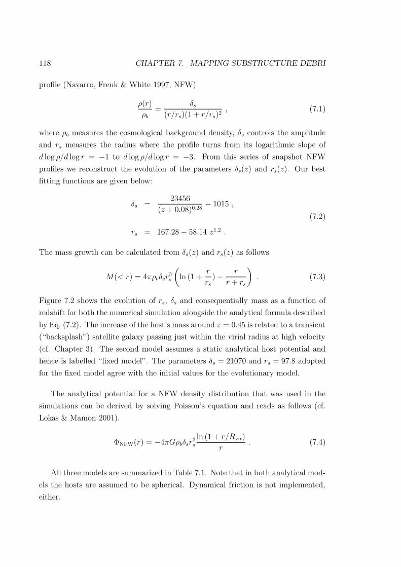
118 CHAPTER 7. MAPPING SUBSTRUCTURE DEBRI
profile (Navarro, Frenk & White 1997, NFW)
ρ(r)
ρb
=δs
(r/rs)(1 + r/rs)2, (7.1)
where ρb measures the cosmological background density, δs controls the amplitude
and rs measures the radius where the profile turns from its logarithmic slope of
d log ρ/d log r = −1 to d log ρ/d log r = −3. From this series of snapshot NFW
profiles we reconstruct the evolution of the parameters δs(z) and rs(z). Our best
fitting functions are given below:
δs =23456
(z + 0.08)0.28− 1015 ,
rs = 167.28 − 58.14 z1.2 .
(7.2)
The mass growth can be calculated from δs(z) and rs(z) as follows
M(< r) = 4πρbδsr3s
(
ln (1 +r
rs
) − r
r + rs
)
. (7.3)
Figure 7.2 shows the evolution of rs, δs and consequentially mass as a function of
redshift for both the numerical simulation alongside the analytical formula described
by Eq. (7.2). The increase of the host’s mass around z = 0.45 is related to a transient
(“backsplash”) satellite galaxy passing just within the virial radius at high velocity
(cf. Chapter 3). The second model assumes a static analytical host potential and
hence is labelled “fixed model”. The parameters δs = 21070 and rs = 97.8 adopted
for the fixed model agree with the initial values for the evolutionary model.
The analytical potential for a NFW density distribution that was used in the
simulations can be derived by solving Poisson’s equation and reads as follows (cf.
Lokas & Mamon 2001).
ΦNFW(r) = −4πGρbδsr3s
ln (1 + r/Rvir)
r. (7.4)
All three models are summarized in Table 7.1. Note that in both analytical mod-
els the hosts are assumed to be spherical. Dynamical friction is not implemented,
either.

7.2. THE HOST HALO AND SATELLITE GALAXY 119
Figure 7.2: The evolution of the Host Halo
The redshift dependence for rs (upper panel), δs (middle panel) and consequentiallyvirial mass, Mvir (lower panel). The solid lines indicate the evolution in the livemodel, and the dashed lines are our best fitting formula to describe the evolution(see eq. 7.2).

120 CHAPTER 7. MAPPING SUBSTRUCTURE DEBRI
Table 7.1: Summary and nomenclature for the four models. The disruption times andnumber of full orbits are for the modelled satellite galaxy.
Model δs rs [h−1 kpc]
live solid lines in Figure 7.2evolutionary as given by Eq. (7.2)
fixed 21070 97.8
7.3 Real-Space Properties
In Figure 7.3 we show the real-space distribution of the disrupted satellite after
the 8.3 Gyrs evolution, i.e. at z = 0. Figure 7.4 shows the distance of the satellite
galaxy to the host as a function of time. The spread in the number of orbits amongst
the models can readily ascribed to the difference in host mass and the small “mis-
modelling” of its growth as seen in Figure 7.2 at around redshift z = 0.3.
These figures further highlight a number of interesting differences and similarities
amongst the models. The most striking feature is that neither of the analytical
models is capable of producing the real-space distribution of particles seen in the
live model, and the live model shows the most “compact” distribution. Although all
models display “shell”-like features, they are less eminent for the live host. Instead,
the live model exhibits a “cross-like” feature and appears to be more compact in
the central region, respectively. A comparable feature, in fact, has also been noted
in observational streams (cf. Hau et al. 2005).
7.4 Integral-Space Properties
Helmi & de Zeeuw (2000) outlined a method for identifying stellar streams within ob-
servational data sets by utilising conservation of energy, E, and angular momentum,
L, (i.e. the integrals-of-motion) for spherically symmetric and time-independent po-
tentials. In fact, this method proved to be a powerful tool for identifying streams in
the Milky Way using the proper motions of solar neighbour stars (Helmi et al. 1999;
Chiba & Beers 2000; Brook et al. 2003; Navarro, Helmi & Freeman 2004). We
expand their analysis not only limiting ourselves to static analytical models but
extending the study to include both our live and evolutionary models.
The integrals of motion, total energy Ei = Ti +Ui and angular momentum ~Li for
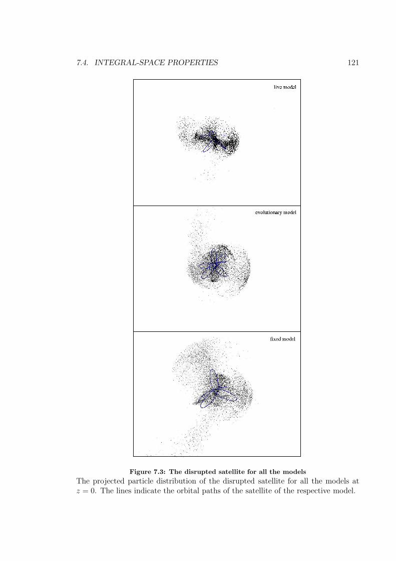
7.4. INTEGRAL-SPACE PROPERTIES 121
Figure 7.3: The disrupted satellite for all the models
The projected particle distribution of the disrupted satellite for all the models atz = 0. The lines indicate the orbital paths of the satellite of the respective model.

122 CHAPTER 7. MAPPING SUBSTRUCTURE DEBRI
Figure 7.4: The orbit of the satellite galaxy.
The distance of the satellite galaxy to the host as a function of time.

7.4. INTEGRAL-SPACE PROPERTIES 123
Figure 7.5: Distributed satellites in integral space for the live model
The distribution of satellite particles in the E − L plane for the live model. Thebottom panel shows the distributions at the time the respective satellite galaxyenters the virial radius of the host whereas the top panel presents the distributionsat z = 0. Different colours represent particles of different satellites.

124 CHAPTER 7. MAPPING SUBSTRUCTURE DEBRI
each satellite particle i with respect to the host halo is calculated as follows. For the
two analytical NFW potential models, we simply use Eq. (7.4) as the contribution
from the host to the potential energy Ui, but for the live model we adhere to the
following:
Φlive(r) = −G
(
M(< r)
r+
Mvir
Rvir
gc
1 + r/rs
)
, (7.5)
where g = [log (1 + c)−c/(1+c)]−1 and c = Rvir/rs measures the concentration. This
formula is also based upon the assumption that the halo is spherically symmetric
but provides a reasonable approximation. The potential energy contribution from
the host therefore reads
Uhosti = mi
Φlive(ri), for the live model
ΦNFW(ri), for all other models(7.6)
This potential energy, however, is further augmented by the contribution from the
self-gravity of the satellite which is derived via straight forward summation U satI .
Thus the total potential energy of a single satellite particle is given by Ui = Uhosti +
U satI . The kinetic energy and angular momentum are calculated in the obvious way
with respect to the host.
We like to stress that integrals of motion are associated with symmetries and
cyclic coordinates in the Hamiltonian, respectively. For a static and spherically
symmetric potential the Hamiltonian does not explicitly depend on time and the
angles θ or φ which results in energy and angular momentum conservation. Yet this
ideal situation is not even satisfied for the fixed model since the contribution from
the self-gravity violates angular momentum conservation; we should observe energy
conservation though. However, conservation of energy and/or angular momentum
should not be taken for granted. If observed, it simply indicates that the self-
gravity of the satellite (and the time evolution of the potential) makes an overall
small contribution to the Hamiltonian.
7.4.1 The evolution in the E − L plane for the live model
Before exploring the evolution in the E − L plane (hereafter also called “integral-
space”) of our target satellite in all three models, we present the evolution for eight
different satellites in the live model alone. The result can be viewed in Figure 7.5
where each satellite is represented by an individual colour with our target satellite

7.4. INTEGRAL-SPACE PROPERTIES 125
plotted as cyan. The satellites shown in Figure 7.5 are all taken from the self-
consistent cosmological simulation and represent a fair sample of all 158 available
satellites, i.e. their masses cover a range from M ∼ 5 × 10¹⁰h−1 M to M ∼4× 10¹²h−1 M and they are on different orbits. The left panel of Figure 7.5 shows
the distributions at the time the satellite enters the virial radius of the host, whereas
the right panel displays the distributions at z = 0.
Figure 7.5 allows us to gauge the “drift” of satellites in integral-space. We note
that, compared to Figure 4 of Helmi & de Zeeuw (2000), the integrals-of-motion are
hardly conserved in the live model, neither for high or low mass streamers. The
distributions rather show a large scatter, and have been significantly “re-shaped”
over time. In addition, the mean values of E and L are also moved after the evolu-
tion. For instance, the “red” satellite drifts in time over to the initial position of the
“cyan” satellite. Figure 7.5 further demonstrates that the drift of our target satellite
(cyan dots) is comparable to the evolution of the other satellites, thus indicating
that this target satellite is a “typical satellite” in that respect.
One encouraging result implied from Figure 7.5, however, is that even though
the integrals-of-motion are changing over time, satellites still appear coherent in the
E − L plane. Hence, the integral-space analysis pioneered by Helmi & de Zeeuw
(2000) still proves to be a useful diagnostic to identify streams. We further like
to stress that observations only provide us with the snapshot of the distribution at
today’s time, i.e. the right hand panel of Figure 7.5 and hence measuring “evolution”
is beyond the scope of RAVE and GAIA.
7.4.2 The evolution in the E − L place for all models
Figure 7.6 now focuses on our target satellite alone, showing its particles at initial
and final time in the E − L plane for all three models, i.e. the live, evolutionary
and fixed model. We notice that particles tend to form “stripes” in the E −L plane
(parallel to the L-axis) indicative of a spread in angular momentum for particles
of comparable energy. These stripes form over time and have been directly linked
to both apo- and peri-centre passages of the satellite. The live model deviates
most prominently from the other models not only reducing total energies, but also
“randomising” the angular momentum and hence lacking the prominence of these
stripes. We also observe in Figure 7.6 that the fixed model is the only model to show
a noticeable number of particles (≈ 3%) not bound to the host halo, i.e. E > 0.

126 CHAPTER 7. MAPPING SUBSTRUCTURE DEBRI
Figure 7.6: The evolution in the E − L place for all models
Total energy, E, versus absolute value of the angular momentum, L, for all satelliteparticles within the target satellite at initial redshift z = 1.16 (black) and at z = 0(purple) in the live (bottom), evolutionary (middle) and fixed (top) models. Thehorizontal line indicates E = 0.
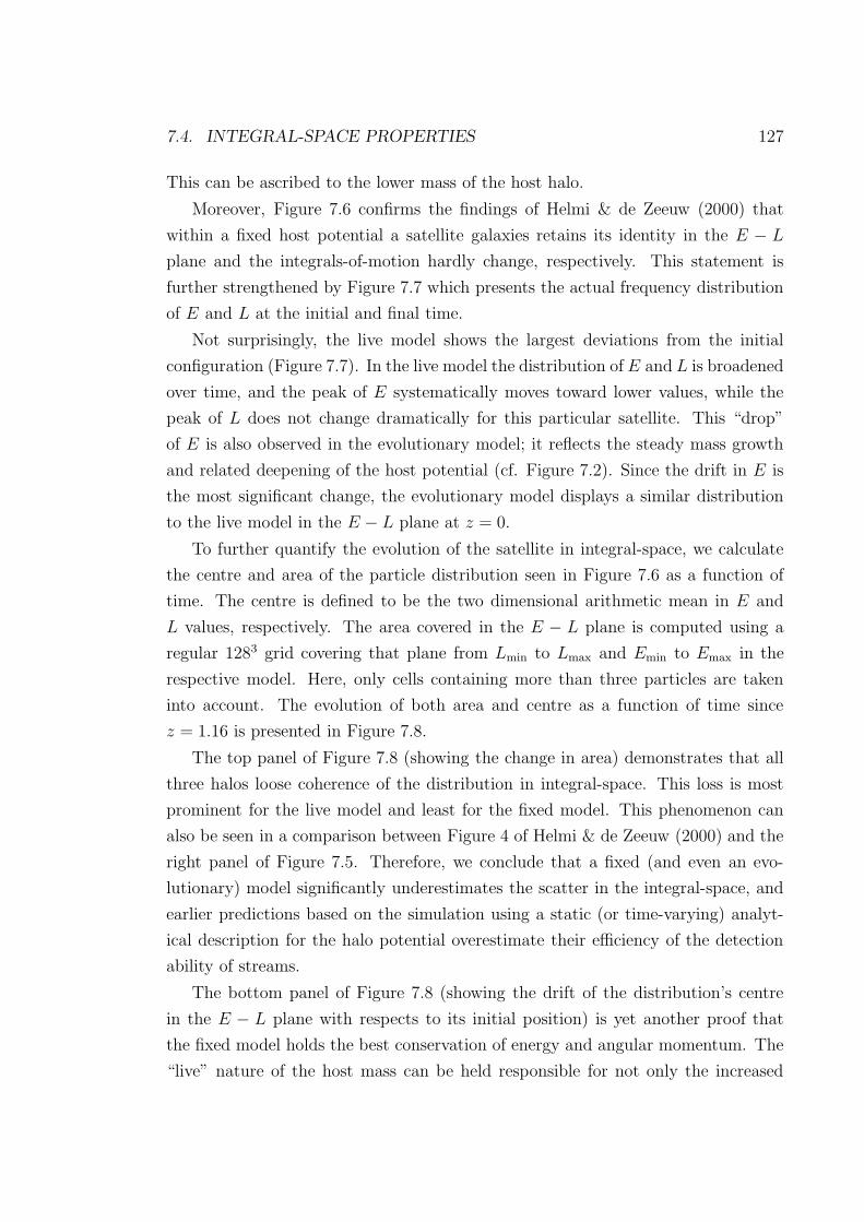
7.4. INTEGRAL-SPACE PROPERTIES 127
This can be ascribed to the lower mass of the host halo.
Moreover, Figure 7.6 confirms the findings of Helmi & de Zeeuw (2000) that
within a fixed host potential a satellite galaxies retains its identity in the E − L
plane and the integrals-of-motion hardly change, respectively. This statement is
further strengthened by Figure 7.7 which presents the actual frequency distribution
of E and L at the initial and final time.
Not surprisingly, the live model shows the largest deviations from the initial
configuration (Figure 7.7). In the live model the distribution of E and L is broadened
over time, and the peak of E systematically moves toward lower values, while the
peak of L does not change dramatically for this particular satellite. This “drop”
of E is also observed in the evolutionary model; it reflects the steady mass growth
and related deepening of the host potential (cf. Figure 7.2). Since the drift in E is
the most significant change, the evolutionary model displays a similar distribution
to the live model in the E − L plane at z = 0.
To further quantify the evolution of the satellite in integral-space, we calculate
the centre and area of the particle distribution seen in Figure 7.6 as a function of
time. The centre is defined to be the two dimensional arithmetic mean in E and
L values, respectively. The area covered in the E − L plane is computed using a
regular 1283 grid covering that plane from Lmin to Lmax and Emin to Emax in the
respective model. Here, only cells containing more than three particles are taken
into account. The evolution of both area and centre as a function of time since
z = 1.16 is presented in Figure 7.8.
The top panel of Figure 7.8 (showing the change in area) demonstrates that all
three halos loose coherence of the distribution in integral-space. This loss is most
prominent for the live model and least for the fixed model. This phenomenon can
also be seen in a comparison between Figure 4 of Helmi & de Zeeuw (2000) and the
right panel of Figure 7.5. Therefore, we conclude that a fixed (and even an evo-
lutionary) model significantly underestimates the scatter in the integral-space, and
earlier predictions based on the simulation using a static (or time-varying) analyt-
ical description for the halo potential overestimate their efficiency of the detection
ability of streams.
The bottom panel of Figure 7.8 (showing the drift of the distribution’s centre
in the E − L plane with respects to its initial position) is yet another proof that
the fixed model holds the best conservation of energy and angular momentum. The
“live” nature of the host mass can be held responsible for not only the increased
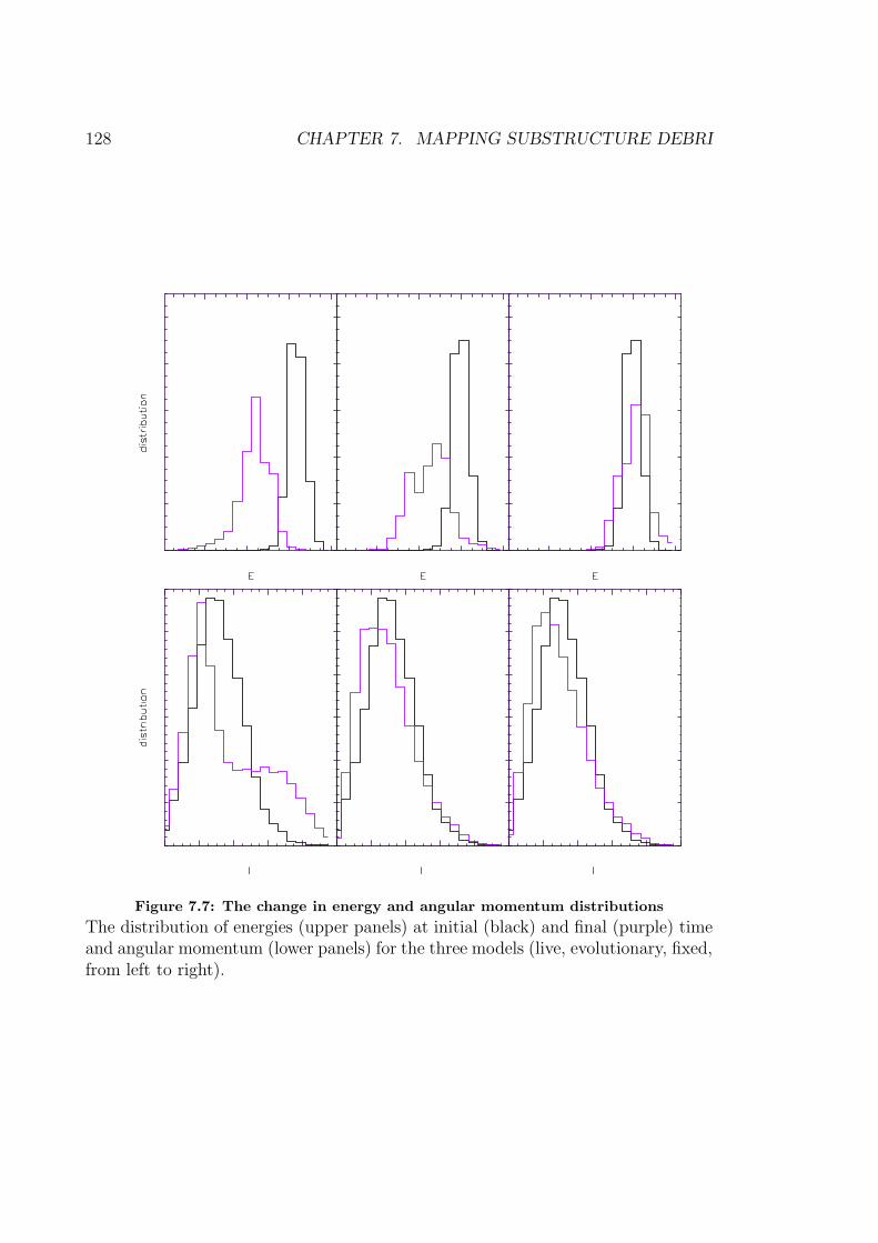
128 CHAPTER 7. MAPPING SUBSTRUCTURE DEBRI
Figure 7.7: The change in energy and angular momentum distributions
The distribution of energies (upper panels) at initial (black) and final (purple) timeand angular momentum (lower panels) for the three models (live, evolutionary, fixed,from left to right).
7.4. INTEGRAL-SPACE PROPERTIES 129
Figure 7.8: The time evolution of the disrupted satellite in integral-space
The evolution of the area (top panel) and the centre (bottom panel) in integral-space(see text for more details) as a function of time for the live (solid), evolutionary (dot-dashed) and fixed (dotted line) models.

130 CHAPTER 7. MAPPING SUBSTRUCTURE DEBRI
dispersion (i.e. area) but also for the actual drift in integral-space. We further like
to stress that at no time the evolutionary model matches the effects of the “live”
model. There always appears to be a well pronounced discrepancy which can be
ascribed to effects not considered in the evolutionary model, such as the triaxiality
of the host and interactions of the debris with other substructure. This leads to
the immediate conclusion that for an understanding of the formation of streams
in integrals-of-motion space it appears rather crucial to take into account the full
complex evolutionary effects of the host. The first such step has been taken by
Zhao et al. (1999) who modelled the evolution of tidal debris in a time-varying
potential. However, our study further indicates that in a “live” scenario there are
additional effects at work leading to an even greater dispersion.
7.5 Conclusions
As we have seen in Chapter 1 in the hierarchical structure formation scenario Dark
Matter halos continuously grow via both merger activity and steady accretion of
material. Furthermore, they also contain a great deal of substructure and are far
from spherical symmetry. We have investigated the development of streams due to
the tidal disruption of satellite galaxies in a DM halo forming in a fully self-consistent
cosmological simulation. This not only models the time-dependency of the potential
(reflecting the mass growth of the host), it also accounts for other effects such as
the triaxiality of the host and interactions of the debris with other satellites.
Our conclusions can be summarised as follows. (1) The distributions of (debris
of) satellite galaxies in both real and integrals-of-motion space are sensitive to the
evolution (and the particulars) of their host galaxy. This puts a caution on studies
that investigate the shape of the halo based on satellite streams obtained via simu-
lations with static DM halos. (2) Even in a ΛCDM “live” halo, satellites still appear
to be coherent structures in the integrals-of-motion space. However, the coherency
is smeared significantly in contrast to predictions from simulations using static and
time-varying host potentials, respectively. Thus, earlier studies of the detection
ability of streams using a static DM potentials (Helmi & de Zeeuw 2000; Harding
et al. 2001) and even time-varying potentials (Zhao et al. 1999) could overestimate
the efficiency of the “integrals-of-motion approach”. (3) In the integrals-of-motion
space, energy changes most significantly due to the mass growth of the host halo
7.5. CONCLUSIONS 131
which is inevitable in hierarchical structure formation scenarios. However, there
are additional effects at work such as triaxiality of the host and interactions of the
stream with other satellites. Hence, any currently observed distribution of a satellite
stream in the E − L plane no longer reflects its original distribution.

132 CHAPTER 7. MAPPING SUBSTRUCTURE DEBRI

Chapter 8
Conclusions and Future Directions
“Between the traditional and the new, or between order
and adventure, there is no real opposition; and what we calltradition today is a knit work of centuries of adventure.”
- Jorge Luis Borges
8.1 Conclusion
Dark matter substructure is believed to be an integral component to galaxy and
galaxy cluster formation and evolution. Throughout this thesis we have used nu-
merical simulations to complete a number of studies that look at the evolution and
fate of dark matter substructure.
Chapter 2: Simulations
MLAPM (Knebe, Green & Binney 2001) is an N-body solver that uses an adaptive
multi grid approach to simulate the formation of structures in the Universe from
collisionless dark matter. Taking advantage of MLAPM’s ability to efficiently and
accurately simulate structure in dense environments through its adaptive grids, we
produced a series of high-resolution ΛCDM cosmological simulations that focused
on the formation and evolution of eight dark matter galaxy clusters, each of order
a million particles within the virial radius. In addition to high mass and spatial
resolution, we also have a substantial number of simulation snapshots and hence are
133

134 CHAPTER 8. CONCLUSIONS AND FUTURE DIRECTIONS
able to follow the evolution of the individual sub-halos as they fall into and orbit
within the global potential of the cluster.
Chapter 3: Finding dark matter halos
To take advantage of data created by sophisticated N -body codes (such as MLAPM),
one needs an equally sophisticated halo finder. In Chapter 3 we introduced our new
”MLAPM-halo-finder” (MHF) which is based on the adaptive grid hierarchy of MLAPM.
In practice, the grid structure of MLAPM adaptively refines around high-density
regions with an automated refinement algorithm. MLAPM creates a hierarchy of re-
finement meshes of differing resolutions closely following the complicated density
distribution of simulation particles (i.e. filamentary structures, walls and, most im-
portantly, gravitationally bound objects). The refinement is done cell-by-cell thus
meshes are not constrained to have a rectangular (or any other) shape. Thus the
grid structure naturally “surrounds” the dark matter halos, as they are simply man-
ifestations of over-densities within (and exterior) to the underlying host halo.
Identifying isolated MLAPM grids we restructure the grid hierarchy into a “grid
tree”. Thus each of the branches of this tree is a ’dark matter halo’. Further,
because of the unconstrained generation of the grids, each branch can have additional
branches, thus identifying sub-sub-halos. This embedded-halo-within-halo scenario
is limited only by the simulation resolution.
However, this method proved insufficient to find all sub-halos against the high
background density in the innermost regions of the hosts. To overcome this ob-
stacle we developed “MLAPM-halo-tracker” (MHT) which augmented the halo finder
by incorporating information from multiple simulation timesteps. MHT allowed us
to track the orbital evolution of gravitationally-bound objects through any given
cosmological N -body-simulation.
Using both MHF and MHT we followed the temporal evolution of hundreds of
individual satellites within their host halos. This excellent data set allowed us to
perform the investigations described in Chapters 4-7.
Chapter 4: The dynamics of substructure
Our eight dark matter galaxy clusters (host halos) were chosen to sample a variety
of formation histories, ages, and triaxialities. Despite their obvious differences, we
have found striking similarities between their sub-halo populations.
8.1. CONCLUSION 135
Surprisingly, between each of the clusters the substructure populations of each
host had an average eccentricity of ∼ 0.6 and an average peaked pericentre of 35% of
the cluster radius. We also found similar rates of sub-galaxy disruption for all galaxy
clusters, which is not surprising considering the similarity in the orbital distributions.
Specifically we found that the disrupted sub-galaxies were on more circular orbits,
and thus that they experienced stronger tidal forces for longer periods.
Within our cluster simulations we also found that the velocity dispersion of the
sub-galaxies was greater than the velocity dispersion of the actual galaxy cluster,
implying that the sub-galaxies do not ideally reflect the underlying cluster. This
result is significant because one popular method of measuring the mass of a cluster is
based on the velocity dispersion of the sub-galaxies. However, our results found that
this leads to an over-estimation of the cluster mass due to the mismatch in velocity
dispersion. When we restricted the calculation of the sub-galaxy velocity disper-
sion to those sub-galaxies having more than one orbital period, this difference was
essentially removed, and the sub-galaxies reflected the dynamics of the underlying
cluster.
In summary, we found that all the properties of the sub-galaxy populations
appear to be independent of the galaxy cluster and its history. We were unable
to identify any trends with richness, triaxiality and/or formation time (other than
the number of orbits) thus exhibiting a high level of self-similarity between the
sub-galaxy populations.
Chapter 5: Anisotropy of substructure orbits
There is strong observational evidence on scales spanning from galaxy clusters down
to galaxies there is a signal indicating a correlation between the alignment of sub-
structure and the shape of the gravitational potential this substructure moves in.
Using our cluster simulations we proposed a possible explanation for the controversy
regarding the alignment of sub-halos orbits within dark matter halos.
Specifically we found that the apocentres of the orbits of these satellites lie
preferentially within a cone of opening angle ∼40 around the major axis of the host
halo, in accordance with the observed anisotropy found in galaxy clusters. We do,
however, note that a link to the dynamical age of the cluster is not well established
as both our oldest dark matter halos show a clear anisotropy signal. Further analysis
connects this distribution to the infall pattern of satellites along the filaments: the

136 CHAPTER 8. CONCLUSIONS AND FUTURE DIRECTIONS
orbits are determined by the environment of the host halo rather than by some
”dynamical selection” during their life within the host’s virial radius.
Chapter 6: Outskirts of dark matter halos
In addition to investigating the dynamics of sub-galaxies within the galaxy cluster,
we also investigated galaxy populations in the outskirts of galaxy clusters.
It has been known for quite some time that galaxy properties in clusters are
substantially different from galaxies in the field. However, the origin of the so-
called ‘morphology-density’ relationships are still not fully understood, with several
large and small-scale mechanisms proposed to explain their existence, including ram
pressure stripping, tidal stripping/star formation, starvation, galaxy mergers and
harassment and dynamics.
Using our simulations we demonstrated that a rich population of galaxies exists
beyond the virial radius that at one stage had spent time near the cluster centre (i.e.
“backsplash” galaxies). Hence, this needs to be appreciated when interpreting the
various galaxy morphology environmental relationships and decoupling the degener-
acy between nature and nurture. Specifically, we have found that approximately half
of the galaxies with current cluster-centric distances in the range 1 – 2 virial radii of
the host were “backsplash” and that 90% of these had penetrated to within 50% of
the virial radius. As a result they had undergone significant tidal disruption, losing
on average 40% of their mass. Furthermore, we believe that these backsplash galax-
ies are kinematically distinct and should be observable within existing spectroscopic
surveys.
Chapter 7: Mapping substructure debris
As we have seen in the introduction and Chapter 2, within the hierarchical structure
formation paradigm galaxies/clusters are built by the continuous accretion of smaller
objects. The disruption of these smaller galaxies within the (newly formed) larger
halos results in the creation of stellar streams, the most spectacular of these in the
Milky Way being the Sagittarius stream (Ibata 2001c).
Through this study we presented a detailed study of the real and integrals-of-
motion space distributions of a disrupting satellite obtained from one of our fully self-
consistent high-resolution cosmological simulation of a galaxy cluster. In addition,
the satellite was re-simulated using various analytical halo potentials. We found

8.2. FUTURE DIRECTIONS 137
that its debris appears as a coherent structure in integrals-of-motion space in all
models (“live” and analytical potential) although the distribution is significantly
smeared for the live host halo. The primary mechanism for the dispersion is the
mass growth of the host. However, when quantitatively comparing the effects of
“live” and time-varying host potentials we conclude that not all of the dispersion can
be accounted for by the steady growth of the host’s mass. We ascribe the remaining
discrepancies to additional effects in the “live” halo such as non-sphericity of the host
and interactions with other satellites, which have not been modelled analytically.
8.2 Future Directions
Galaxy clusters are well-defined astrophysical objects that can be readily observed.
However, there still remain numerous outstanding questions regarding their ori-
gins and properties. Currently, and in the future, I am interested in investigating
(through numerical simulations) a number of important questions regarding the evo-
lution of substructure and their tidal debris. A sample of these ongoing and planned
investigations include:
Satellite-Satellite interaction
There are many mechanisms to transform a galaxy. Over the past decade there has
been a great deal of work that aimed to quantify the effects of various transforma-
tion mechanisms, for example, the ram-pressure stripping of a galaxy’s reservoir of
gas by the hot intracluster medium. However, other mechanisms, such as sub-halo
– sub-halo interactions or “galaxy harassment”, have been paid comparatively little
attention and thus their role in galaxy transformation within clusters is unclear. Are
sub-halo – sub-halo interactions significant and are they sufficient to induce star-
bursts, thus exhausting the galaxies’ reservoirs of gas that fuel their star formation?
This is an outstanding question that we are ideally placed to investigate (through
MHT and simulation data) and to which we can make a timely contribution.
Calculating the shape of the galactic potential using satellite streams
Another direction for future research that follows from my thesis (cf. Chapter 7)
and has timely international recognition largely due to the European Space Agency’s
satellite mission GAIA and the ground based RAVE survey, is the investigation of
138 CHAPTER 8. CONCLUSIONS AND FUTURE DIRECTIONS
stellar streams from disrupting galaxies. As we have previously discussed the signa-
tures of hierarchical galaxy formation are evident in the observed substructure seen
in various phase-space projections of the Galactic halo. Ibata et al. (2001b) using
the Sagittarius stream demonstrated their use in constraining the shape of the halo’s
gravitational potential. In the case of the Milky Way, Ibata et al. concluded that
our halo was necessarily spherical (under the assumption of a static axisymmetric
potential).
However, the current model of the Universe predicts that typical galaxy halos
should be triaxial (Power et al. 2002). Thus, the observation that the Milky Way’s
halo is approximately spherical is difficult to reconcile with our current understand-
ing. It would be interesting to extend the work in Chapter 7 on the identification
of stellar streams and investigate the variance of a stream’s coherence with its host
halo, particularly focusing on effects of the stream in triaxial hosts. As a natural
extension, we would address the question of what shape would be inferred for a
cosmological halo by tracking the stellar debris, and how would it compare with the
‘true’ (or measured) shape?
Modelling galaxy clusters
Thus far we have studied in detail the gravitational dynamics of galaxy clusters.
However, if we wish to better understand galaxy transformation in clusters, it is
imperative that we relate our numerical models to the observational data. One
potentially powerful way to achieve this is through the inclusion of baryonic physics
in the cosmological (dark matter) simulations. There are a number of different ways
to do this.
In the short term we aim to produce a modularised open source semi-numerical
code. Unlike semi-analytic simulations that describe halo mass growth through
analytical calculations based upon linear perturbation theory (Press & Schechter
1974), semi-numerical simulations use the dynamical information from N -body sim-
ulations. Both methods, however describe the baryonic physics through an analytic
formalism. This method has many advantages, the first and foremost being that
it is computationally inexpensive. This provides a user with a controlled way to
investigate their research problem and explore a larger range in parameter space.
An example of the benefits of a semi-numeric approach is demonstrated in the
interpretation of the anti-bias found in the sub-halo density profile, an anti-bias

8.2. FUTURE DIRECTIONS 139
that does not exist in observational data (cf. Chapter 4). Through the use of semi-
numerical techniques Gao et al. (2004) were able to account for this discrepancy.
Their conclusion was that tidal stripping of the dark sub-halos was very efficient
in reducing their mass while having less of an effect on the tightly bound baryonic
galaxy at its core. Thus, while the dark matter sub-halos in the inner regions of the
cluster were being disrupted, their baryonic galaxies survived. (Note: such disrupted
galaxies must be old).
Thus one natural extension of my research would be to build on the development
of MHF and in particular MHT (tracker), which follows the galaxy dynamics and cou-
pling it to a semi-analytical treatment, thus developing a semi-numerical code. Such
a union would produce a powerful tool, which could be used to address questions
regarding galaxy transformation, and to investigate broader questions such as the
nature of various galaxy morphology relationships. For example, supplementing the
kinematic information from the N -body simulations by producing colour and surface
brightness distributions, thus assiting in the empirical identification of backsplash
galaxies.
While these semi-numerical techniques are powerful, in the long run it is our aim
to add hydrodynamics and baryonic physics into MLAPM. Although this problem is
more computationally expensive and is more technically challenging, the gains from
an ‘’unbiased” transformation into the observer’s plane are significant.
With respects to modelling galaxy clusters, ultimately it is our aim to grow
a suite of open source programmes that investigate cluster and galaxy evolution
that are easy to use and take great care in transforming simulation data in to the
observers plane.

140 CHAPTER 8. CONCLUSIONS AND FUTURE DIRECTIONS
“A humble peasant who serves God is much more
pleasing to him than an arrogant academic who neglects hissoul to consider the course of the stars”
- Thomas a Kempis
141

142 CHAPTER 8. CONCLUSIONS AND FUTURE DIRECTIONS

“When the Sun shrinks to a dull red dwarf, it will not be
dying. It will just be starting to live and everything that hasgone before will merely be a prelude to its real history.”
- Arthur C. Clarke
143

144 CHAPTER 8. CONCLUSIONS AND FUTURE DIRECTIONS
Bibliography
[1] Aarseth S.J., MNRAS 126, 223 (1963)
[2] Aguerri J.A.L., Iglesias-Paramo J., Vilchez J.M., Munoz-Tunon C.,
ApJ 127, 1344 (2004)
[3] Arp H., PASP, 80, 129, (1968)
[4] Bahvsar S., ApJ 246, L5 (1981)
[5] Bailin J., Steinmetz M., Astron. J. 27, 616 (2004)
[6] Balogh M.L., Navarro J.F., Morris S.L., ApJ 540, 113 (2000)
[7] Barnes J.E., Hut P., Nature 324, 446 (1986)
[8] Bekki K., Couch W.J., Drinkwater M.J., Shioya Y., MNRAS 344, 399 (2003)
[9] Bertschinger E., Gelb J.M., Computers in Physics 5, 164 (1991)
[10] Bingegeli B., Tammann G.A., Sandage A., Astron. J. 94, 251 (1987)
[11] Bingelli B. 1999, in The Radio Galaxy Messier 87, ed. H.J. Roser & K. Meisen-
heimer (Berlin: Springer), 9
[12] Binney J., Tremaine S., Galactic Dynamics, Princeton: Princeton University
Press, (1987)
[13] Bode P., Ostriker J.P., Turok N., ApJ 539, 93 (2001)
[14] Bullock J., Kravtsov A., Weinberg D., ApJ 539, 517 (2000)
[15] Bullock J., Kolatt T.S., Sigad Y., Sommervile R.S., Kravtsov A.V., Klypin
A.A., Primack J.R., Dekel A., MNRAS 559, 321 (2001)
145

146 BIBLIOGRAPHY
[16] Brainerd T.G., astro-ph/0408559
[17] Brandt A., Math. Comput., 31, 333, (1977)
[18] Brook C.B., Kawata D., Gibson B.K., Flynn C., ApJ 585, L125 (2003)
[19] Bryan G.L., Norman M.L., ApJ 495, 80 (1998)
[20] Butcher H., Oemler A., ApJ 226, 559 (1978)
[21] Calcaneo-Roldan C., Moore B., Bland-Hawthorn J., Malin D., Sadler E.M.
MNRAS 314, 324 (2000)
[22] Carlberg R. G., ApJ 433, 368 (1994)
[23] ChaboyerB., DemarqueP., KernanP.J., KraussL.M., ApJ 494, 96 (1998)
[24] Chiba M., Beers T.C., Astron. J. 118, 2843 (2000)
[25] Colberg J.M., White S.D.M., Jenkins A., Pearce F.R., MNRAS 593, 308 (1999)
[26] Cole S., Lacey C., MNRAS 281, 716 (1996)
[27] Colin P., Avila-Reese V., Valenzuela O., ApJ 542, 662 (2000)
[28] Colin P., Klypin A., Kravtsov A., Khokhlov A., ApJ 523, 32 (1999)
[29] Colless M., et al. VizieR On-line Data Catalog 226, 7226, (2003)
[30] Colless M., et al. MNRAS 328, 1039 (2001)
[31] Connors T.W., Kawata D., Maddison S.T., Gibson B.K.,
Pub. Astron. Soc. Aust. D21, 222 (2004)
[32] Dahle H., Hannestad S., Sommer-Larsen J., ApJ 588, 25 (2003)
[33] Dalal N., Kochanek C. S., ApJ 572, 25 (2002)
[34] Davis M., Efstathiou G., Frenk C.S., White S.D.M., ApJ 292, 371 (1985)
[35] deBernardisP., et al. Nature 404, 955 (2000)
[36] de Lucia G., Kauffmann G., Springel V., White S., astro-ph/0306205
[37] de Souza R.E., Capelato H.V., Arakaki L., Logullo C., ApJ 263, 557 (1982)
BIBLIOGRAPHY 147
[38] Dressler A., ApJ 236, 351 (1980)
[39] Dubinski J., Carlberg R. G., ApJ 496, 378 (1991)
[40] Efstathiou G., Davis M., Frenk C.S., White S.D.M., ApJ Suppl. 57, 241 (1985)
[41] EkeV.R., Cole S., Frenk C.S., MNRAS 282, 263 (1996)
[42] Evans N.W., Witt H.J., MNRAS 345, 1351 (2003)
[43] Faltenbacher A., Gottlber S., Kerscher M., Mller V., A&A 359, 1 (2002)
[44] Feldmeier J.J., Mihos C., Morrison H.L. Rodney S., Harding P.,
ApJ 575, 779 (2002)
[45] Franx M., Illingworth G., de Zeeuw T., ApJ 383, 112 (1991)
[46] Freeman K.C., 1996, in ASP Conf. Proc. 92, Formation of the Galactic Halo -
Inside and Out, ed. H. Morrison & A. Sarajedini (San Francisco: ASP), p.3
[47] Frenk C.S., White S.D.M., Davis M., Efstathiou G., ApJ 327, 507 (1988)
[48] Gardiner L.T., Noguchi M., MNRAS 278, 191 (1996)
[49] GarnavichP.M., JhaS., ChallisP., ClocchiattiA., DiercksA., FilippenkoA.V.,
GillilandR.L., Astron. J. 509, 74 (1998)
[50] Ghigna S., Moore B., Governato F., Lake G., Quinn T., Stadel J.
MNRAS 300, 146 (1998)
[51] Ghigna S., Moore B., Governato F., Lake G., Quinn T., Stadel J.
MNRAS 544, 616 (2000)
[52] GibsonB.K., StetsonP.B., FreedmanW.L., MouldJ.R., KennicuttR.C.Jr.,
HuchraJ.P., et al. ApJ 529, 723 (2000)
[53] Gill S.P.D., Knebe A., Gibson B.K. MNRAS 351, 399 (2004a)
[54] Gill S.P.D., Knebe A., Gibson B.K., Dopita M.A., MNRAS 351, 410 (2004b)
[55] Gill S.P.D., Knebe A., Gibson B.K., IAU Colloquium #195 280 (2004)
[56] Gill S.P.D., Knebe A., Gibson B.K., MNRAS 356, 1327 (2005)
148 BIBLIOGRAPHY
[57] Gilmore G., Wyse R.F.G., Norris J.E., ApJ Lett. 574, 39 (2003)
[58] Gingold R.A., Monaghan J.J., MNRAS 181, 375 (1977)
[59] Gleb J. M., Bertschinger E., ApJ 436, 467 (1994)
[60] Goto T., Yamauchi C., Fujita Y., Okamura S., Sekiguchi M., Smail I., Bernardi
M., Gomez P., MNRAS 346, 601 (2003)
[61] Gotz M., Huchra J. P., Branderberger R. H., astro-ph/9811393
[62] Grebel E.K., Kolatt T., Brandner W., 1999, in The stellar content of the Local
Group, IAU 192, eds. P. Whitelock & R. Cannon, San Francisco: ASP Conf.
Series
[63] Gregg M.D., West M.J. Nature 396, 549 (1998)
[64] Groth J. E., Peebles P. J. E., ApJ 217, 385 (1977)
[65] Gunn J.E., Gott R.J., ApJ 176, 1 (1972)
[66] Harding P., Morrison, H.L., Olszewski E.W., Arabadjis J. Mateo M., Dohm-
Palmer R.C., Freeman K.C., Norris J.E., ApJ 122, 1397 (2001)
[67] Hartwick F.D.A. 1996, in Proc. IAU Symp. 169, Unresolved Problems of the
Milky Way, ed. L. Blitz & P. Teuben (Dordrecht: Kluwer), 669
[68] Hashimoto Y., Funato Y., Makino J., ApJ 582, 196 (2003)
[69] Hatton S., Ninin S., MNRAS 576, 322 (2001)
[70] Hau G., Gill S.P.D., Knebe A., Gibson B.K., 2005 in preparation
[71] Hayashi E., Navarro J., Taylor J., Stadel J., Quinn T., ApJ 584, 541 (2003)
[72] Heisler J., Tremaine S., Bahcall J., N., ApJ 298, 8 (1985)
[73] Helmi A., White S.D.M., de Zeeuw P.T., Zhao, H., Nature 402, 53 (1999)
[74] Helmi A., de Zeeuw P.T., MNRAS 319, 657 (2000)
[75] Holmberg E., Ark. Astron., 5, 305, (1969)
[76] Hubble E., Humason M.L., ApJ 74, 43 (1931)
BIBLIOGRAPHY 149
[77] Ibata R.A., Irwin M.J., Lewis G.F., Ferguson A.M.N., Tanvir N.R.,
Nature 412, 49 (2001a)
[78] Ibata R., Lewis G.F., Irwin M., Totten E., Quinn T., ApJ 551, 294 (2001b)
[79] Ibata R., Irwin,M., Lewis,G.F., Stolte,A., ApJ 547, 133 (2001c)
[80] Ibata R.A., Lewis G.F., Irwin M.J., Cambresy L., MNRAS 332, 921 (2002)
[81] Icke V., A&A 144, 115 (1985)
[82] Iodice E., Arnaboldi M., Bournaud F., Combes F., Sparke L. S., van Driel W.,
Capaccioli M., ApJ 585, 730 (2003)
[83] Jing Y. P., Suto Y., ApJ 538, 574 (2002)
[84] Johnston K.V., Zhao H., Spergel D.N., Hernquist L., ApJ Lett. 512, 109 (1999)
[85] Johnston K., Hernquist L., Bolte M., ApJ 465, 278 (1996)
[86] Katz N., Quinn T., Bertschinger E., Gelb J. M., MNRAS 270, 71 (1994)
[87] Kawata D., Gibson B.K., MNRAS 340, 908 (2003)
[88] Kenney J. D. P., van Gorkom J. H., Vollmer B., astro-ph/0403103, 2004,
accepted for ApJ
[89] Kitzbichler M.G., Saurer W., ApJ Lett. 590, 9 (2003)
[90] Klypin A.A., Shandarin, S. F., MNRAS 204, 891 (1983)
[91] Klypin A.A., Holtzman J., astro-ph/9712217
[92] Klypin A. Gottlober S., Kravtsov A., Khoklov A., ApJ 516, 530 (1999a)
[93] Klypin A., Kravtsov A., Valenzuela O., Prada, F., ApJ 522, 82 (1999b)
[94] Kodama T., Bower R. G., MNRAS 321, 18 (2001)
[95] Kojima M., Noguchi M., ApJ 481, 132 (1997)
[96] Knebe A., Green A., Binney J., MNRAS 325, 845 (2001)
[97] KnebeA., DevriendtJ.E.G., MahmoodA., SilkJ., MNRAS 329, 813 (2002)

150 BIBLIOGRAPHY
[98] Knebe A., Gill S.P.D., Gibson B.K., Lewis G.F., Ibata R.A., Dopita M.A.,
ApJ 347, 7 (2004)
[99] Kravtsov A. V., Klypin A. A., Khokhlov A. M., ApJ Suppl. 111, 73 (1997)
[100] Kravtsov A. V., PhD thesis, New Mexico State University, Las Cruces, (1999)
[101] Kravtsov A. V., Gnedin O. Y., Klypin A. A., ApJ submitted,
astro-ph/0401088
[102] Kunkel W.E., Demers S., Roy. Green. Obs. Bull., 182, 241, (1976)
[103] Lacey C., Cole S., MNRAS 271, 676 (1994)
[104] Larson R. B., Tinsley B. M., Caldwell C. N., ApJ 237, 692 (1980)
[105] Lee J., Kang X., astro-ph/0505179
[106] Lewis I., et al. MNRAS 334, 673 (2002)
[107] Lokas L., Mamon A., MNRAS 321, 155 (2001)
[108] Lucy L.B., Astron. J. 82, 1013 (1977)
[109] Lynden-Bell D., Observatory, 102, 202, (1982)
[110] Majewski S.R., Kunkel W.E., Law D.R., Patterson R.J. Polak A.A. et al.,
2005 AJ in press (astro-ph/0403701)
[111] Majewski S.R., ApJ Lett. 431, 17 (1994)
[112] Mamon G. A., Sanchis T., Salvador-Sole E., Solanes M. J.,
A&A 414, 445 (2004)
[113] Matthewson D.S., Clearly M.N., Murray J.D., ApJ 190, 291 (1974)
[114] McConnachie A., Irwin M., Lewis G., Ibata R., Chapman S., Ferguson A.,
Tanvir N., 2004 MNRAS in press (astro-ph/0406055)
[115] McGaughS.S., deBlokW.J.G., ApJ 499, 41 (1998)
[116] Merritt D., ApJ 264, 24 (1983)
[117] Merritt D., ApJ 276, 26 (1984)
BIBLIOGRAPHY 151
[118] Miyazaki S., et al. PASJ 54, 833 (2002)
[119] Monaghan J.J., Ann. Rev. A & A 30, 543 (1992)
[120] Moore B., Katz N., Lake G., Dressler A., Oemler A., Nature 379, 613 (1996)
[121] Moore B., Katz N., Lake G., ApJ 457, 455 (1996)
[122] Moore B., Ghigna S., Governato F., Lake G., Quinn T., Stadel J., Tozzi P.,
ApJ Lett. 524, 19 (1999)
[123] Navarro J., Frenk C.S., White S.D.M., ApJ 462, 563 (1996)
[124] Navarro J., Frenk C.S., White S.D.M., ApJ 490, 493 (1997) (NFW)
[125] Navarro J.F., Helmi A., Freeman K.C., ApJ 601, 43 (2004)
[126] Oemler A., ApJ 194, 1 (1974)
[127] Okamoto T., Habe A., ApJ 516, 591 (1999)
[128] Okamoto T., Nagashima M., ApJ 587, 500 (2003)
[129] Olling R.P. Merrifield M.R., MNRAS 311, 361 (2000)
[130] Onuora L.I., Thomas P.A., MNRAS 319, 614 (2000)
[131] PeacockJ.A., et al. Nature 410, 169 (2001)
[132] Peebles P. J. E., Astron. J. 75, 13 (1970)
[133] Penarubbia J., Kroupa P., Boily C., MNRAS 333, 779 (2002)
[134] PenziasA.A., WilsonR.W., ApJ 142, 419 (1965)
[135] Plionis M., Basilikos S., MNRAS Lett. 329, 47 (2002)
[136] Postman M., Geller M.J., ApJ 281, 95 (1984)
[137] Power C., Navarro J.F., Jenkins A., Frenk C.S, White S.D.M., Springel V.,
Stadel J., Quinn T., astro-ph/0201544
[138] Press W. H., Schechter P., ApJ 303, 425 (1974)

152 BIBLIOGRAPHY
[139] Press W.H., Teukolsky S.A., Vetterling W.T., Flannery B.P., Numerical
Recipes. Cambridge Univ. Press, Cambridge, (1992)
[140] RiessA.G., FilippenkoA.V., ChallisP., ClocchiattiA., DiercksA., Gar-
navichP.M. et al. ApJ 116, 1009 (1998)
[141] Sales L., Lambas D.G., MNRAS 348, 1236 (2004)
[142] Sand D. J., Treu T., Smith G. P., Ellis R. S., astro-ph/0310703
[143] Schechter P.L. Wambsganss J., ApJ 580, 685 (2002)
[144] Scholz R.-D., Irwin M.J., in IAU 161, Wide Field Imaging, eds. H.T.
MacGillivray, (1994)
[145] Solanes J. M., Manrique A., Garcia-Gomez C., Gonzalez-Casado G., Giovanelli
R., Haynes M. P., ApJ 548, 97 (2001)
[146] Spergel D.N., Steinhardt P.J., Phys. Rev. Lett. 84, 3760 (2000)
[147] Spergel D.N., Verde L., Peiris H.V., Komatsu E., Nolta M.R., Ben-
nett C.L., Halpern M., Hinshaw G., Jarosik N., Kogut A., Limon M.,
Meyer S.S., Page L., Tucker G.S., Weiland J.L., Wollack E., Wright E.L.,
ApJ Suppl. 148, 175 (2003)
[148] Splinter R.J., Melott A.L., Linn A.M., Buck C., Tinker J.,
ApJ 479, 632 (1997)
[149] Springel V., White S.D.M., Tormen G., Kauffmann G.,
MNRAS 328, 726 (2001)
[150] Somerville R., ApJ 572, 23 (2002)
[151] StomporR., et al. ApJ 561, 7 (2001)
[152] StraussM.A., WillickJ.A., Phys. Rev. D261, 271 (1995)
[153] Suginohara T., Suto Y., ApJ 396, 395 (1992)
[154] Suisalu S., Saar E., MNRAS 274, 287 (1995)
[155] Summers F., Davis M., Evrard A., ApJ 454, 1 (1995)
BIBLIOGRAPHY 153
[156] Suto Y., Cen R., Ostriker J., ApJ 395, 1 (1992)
[157] Taffoni G., Mayer L., Colpi M., Governato F., MNRAS 341, 434 (2003)
[158] Taylor J. E., Silk J., Babul A., astro-ph/0312086
[159] Thomas P. A. et al. MNRAS 296, 1061 (1998)
[160] Tormen G., MNRAS 290, 411 (1997)
[161] Tormen G., Bouchet F., White S., MNRAS 286, 865 (1997)
[162] Tormen G., Diaferio A., Syer D., MNRAS 299, 728 (1998)
[163] Trentham N., Mobasher B., MNRAS 293, 53 (1998)
[164] Treu T., Ellis R., Kneib J., Dressler A., Smail I., Czoske O.,
ApJ 591, 53 (2003)
[165] Tsuchiya T., Shimada M., ApJ 532, 294 (2000)
[166] Tully B., Somerville R., Trentham N., Verheijen M., ApJ 569, 573 (2002)
[167] van den Bosch F.C., Abel T., Crofts R.A., Hernquist L., Simon D.M.,
ApJ 576, 21 (2002)
[168] van Kampen E., MNRAS 273, 295 (1995)
[169] Villumsen J., V., ApJ Suppl. 71, 407 (1989)
[170] Vollmer B., Braine J., Balkowski C., Cayatte V., Duschl W.J.,
A&A 374, 824 (2001)
[171] Warren M.S., Quinn P.J., Salmon J.K., Zurek W.H., ApJ 399, 405 (1992)
[172] Weinberg D., Hernquist L., Katz N., ApJ 477, 8 (1997)
[173] West M.J., Jones C., Forman W., ApJ Lett. 451, 5 (1995)
[174] West M.J., Blakeslee J.P., ApJ Lett. 543, 27 (2000)
[175] White S.D.M., Rees M. MNRAS 183, 341 (1978)
[176] WhiteS.D.M., NavarroJ.F., EvrardA.E., FrenkC.S., Nature 366, 429 (1993)
154 BIBLIOGRAPHY
[177] Yanny B., Newberg H.J., Grebel E.K., Kent S., Odenkirchen M.
et al. ApJ 588, 823 (2003)
[178] York D.G., et al. Astron. J. 120, 1579 (2000)
[179] Yoshizawa A.M., Noguchi M., MNRAS 339, 1135 (2003)
[180] Zaritsky D., Smith R., Frenk C.S., White S.D.M., ApJ 405, 464 (1993)
[181] Zaritsky D., Smith R., Frenk C.S., White S.D.M., ApJ Lett. 478, 53 (1997)
[182] Zaritsky D., Gonzalez A.H., PASP, 111, 1508, (1999)
[183] ZaroubiS., ZehaviI., DekelA., HoffmanY., KolattT., ApJ 486, 21 (1997)
[184] Zentner A.R., Kravtsov A.V., Gnedin O.Y., Klypin A.A., astro-ph/0502496
[185] Zhao H.S., Johnston K.V., Hernquist L., Spergel D.N., A&A 348, L49 (1999)

Appendices
155


Appendix A
Circularity
We wish to establish a correlation between the circularity and eccentricity
λ =Jsat(E)
Jcirc(E), (A.1)
where Jsat(E) measures the angular momentum of an individual satellite with total
energy E. Jcirc(E) is the corresponding angular momentum for a circular orbit with
the same energy E.
The connection needs to be derived using the fact that both orbits share the
same total energy, so we wish to express E as a function of J in both cases, where
the general expression for E and J reads:
E = 12v2 − GM
r
J = |~r × ~v|(A.2)
Circular Orbits
For a circular orbit we know that |~r × ~v| reduces to
Jcirc = rvcirc (A.3)
as both vectors are always orthogonal. Moreover, the circular velocity is given by
v2circ =
GM
r(A.4)
where M is the total mass of the host halo (assumed to be a point mass).
157
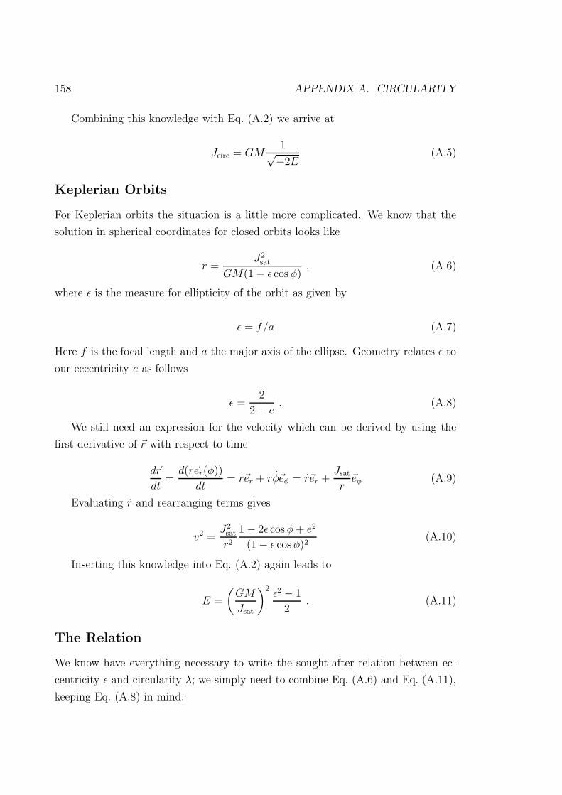
158 APPENDIX A. CIRCULARITY
Combining this knowledge with Eq. (A.2) we arrive at
Jcirc = GM1√−2E
(A.5)
Keplerian Orbits
For Keplerian orbits the situation is a little more complicated. We know that the
solution in spherical coordinates for closed orbits looks like
r =J2
sat
GM(1 − ε cos φ), (A.6)
where ε is the measure for ellipticity of the orbit as given by
ε = f/a (A.7)
Here f is the focal length and a the major axis of the ellipse. Geometry relates ε to
our eccentricity e as follows
ε =2
2 − e. (A.8)
We still need an expression for the velocity which can be derived by using the
first derivative of ~r with respect to time
d~r
dt=
d(r~er(φ))
dt= r~er + rφ~eφ = r~er +
Jsat
r~eφ (A.9)
Evaluating r and rearranging terms gives
v2 =J2
sat
r2
1 − 2ε cos φ + e2
(1 − ε cos φ)2(A.10)
Inserting this knowledge into Eq. (A.2) again leads to
E =
(
GM
Jsat
)2ε2 − 1
2. (A.11)
The Relation
We know have everything necessary to write the sought-after relation between ec-
centricity ε and circularity λ; we simply need to combine Eq. (A.6) and Eq. (A.11),
keeping Eq. (A.8) in mind:
159
ε =2
2 − e
λ =√
1 − ε2
(A.12)
This relation is plotted as a solid line in Figure 4.13.

160 APPENDIX A. CIRCULARITY

Publications


Refereed publications
[1] A. Knebe, S.P.D. Gill, D. Kawata, B.K. Gibson
Mapping substructure in Dark Matter Halos
Mon. Not. R. Astron. Soc. 357, L35 (2005)
[2] S.P.D. Gill, A. Knebe, B.K. Gibson
The evolution of substructure III: the outskirts of clusters
Mon. Not. R. Astron. Soc. 356, 1327 (2005)
[3] S.P.D. Gill, A. Knebe, B.K. Gibson
The dynamics of cluster substructure
IAU Conference Proceedings 195, 280, (2004)
[4] A. Knebe, S.P.D. Gill, B.K. Gibson
Interactions of Satellite Galaxies in Cosmological Dark Matter Halos
PASA - GCDV conference proceedings 21, 216 (2004)
[5] S.P.D. Gill, A. Knebe, B.K. Gibson, M. Dopita
The evolution of substructure II: linking the dynamics to environment
Mon. Not. R. Astron. Soc. 351, 410 (2004)
[6] S.P.D. Gill, A. Knebe, B.K. Gibson
The evolution of substructure I: finding the substructure
Mon. Not. R. Astron. Soc. 351, 399 (2004)
[7] A. Knebe, S.P.D. Gill, B.K. Gibson, R. Ibata, G. Lewis
Anisotropy in satellite distribution
Astrophys. J. Letter 603, 7 (2004)