The Environmental Consequences of Globalization:

A Country-Specific Time-Series Analysis

Jungho Baek

Research Assistant Professor

Department of Agribusiness and Applied Economics

North Dakota Sate University

Email: jungho.baek@ndsu.edu

Phone: (701) 231-7451

Fax: (701) 231-7400

Yong S. Cho

Professor

Department of Food and Resource Economics

Korea University

Email: yscho@korea.ac.kr

Phone: (822) 3290-3037

Won W. Koo

Professor

Department of Agribusiness and Applied Economics

North Dakota Sate University

Email: won.koo@ndsu.edu

Phone: (701) 231-7448

Fax: (701) 231-7400

Selected Paper prepared for presentation at the American Agricultural Economics

Association Annual Meeting, Orlando, FL, July 27-29, 2008

Copyright 2008 by Jungho Baek, Yong S Cho and Won Koo. All rights reserved. Readers

may make verbatim copies of this document for non-commercial purposes by any means,

provided that this copyright notice appears on all such copies.

2

The Environmental Consequences of Globalization:

A Country-Specific Time-Series Analysis

Abstract: The dynamic relationships among trade, income and the environment for

developed and developing countries are examined using a cointegration analysis. Results

suggest that trade and income growth tend to increase environmental quality in developed

countries, whereas they have detrimental effects on environmental quality in most

developing countries. It is also found that for developed countries the causal relationship

appears to run from trade and income to the environment ─ a change in trade and income

growth causes a consequent change in environmental quality, and the opposite

relationship holds for developing countries.

Keywords: Developed countries, Developing countries, Environmental quality,

Globalization, Time-series analysis, Trade

3

INTRODUCTION

One of the most important debates in international trade policy over the last decade has

been the environmental consequences of trade liberalization/globalization (Copeland and

Taylor 1994 and 2004). Proponents of trade liberalization argue that, since environmental

quality is a normal good, trade-induced income growth causes people to increase their

demand for a clean environment, which in turn encourages firms to shift towards cleaner

techniques of production. Thus, free trade provides a win-win situation in the sense that it

improves both environment and economy. Opponents of globalization, on the other hand,

fear that, if production methods do not change, then environmental quality deteriorates as

trade increases the scale of economic activity. Moreover, developing economies tend to

adopt looser standards of environmental regulations to attract more foreign investment.

Trade liberalization thus may lead more growth of pollution-intensive industries in

developing countries as developed countries enforce strict environmental regulations. As

a result, free trade has a significant adverse effect on environmental quality.

Since the seminal work by Grossman and Krueger (1991), many scholars have

attempted to examine the effect of trade openness on the environment.1 For example,

Lucas et al. (1992) investigate the influence of trade openness on the growth rate of toxic

intensity of output. They find that a high degree of restrictive trade policies tends to

increase pollution intensity in fast-growing economies. Gale and Mendez (1998) analyze

the relationship between trade, growth and the environment, and find that an increase in

income has a detrimental effect on environmental quality, but trade effect on pollution is

1 Grossman and Krueger (1991) investigate the environmental impacts of the North American Free Trade

Agreement (NAFTA) in an NBER working paper, which was later published in 1993 (Grossman and

Krueger 1993), and yield two novel results; (1) environmental quality first deteriorates and then improves

with per capita income, which is known as the Environmental Kuznets Curve (EKC), and (2) trade

liberalization tends to improve environmental quality via income growth.

4

not significant. Dean (2002) examines the effect of trade liberalization on environmental

damage. She finds that increased openness to international markets aggravates

environmental damage through the terms of trade, but mitigates it through income growth.

More recently, Frankel and Rose (2005) estimate the effect of trade on the environment

for a given level of income per capita, and conclude that there is little evidence that

openness causes significant environmental degradation.

Previous studies have undoubtedly expanded our understanding of the

environmental consequences of economic growth and international trade. However,

earlier studies have mostly adopted reduced-form models to examine the presence of

significant statistical association of trade openness and income growth with

environmental quality. Little attention has been paid to the causal effects of trade

liberalization and income on the environment (Coondoo and Dinda 2002, Chintrakarn

and Millimet 2006). More specifically, with the treatment of trade and income as being

exogenous variables for their reduced-form models, past studies run the regression of

measures of environmental quality/damage (e.g., sulfur dioxide and carbon dioxide

emissions) on trade openness (usually defined as the sum of exports and imports divided

by GDP) and income (usually per capita GDP). This approach implicitly assumes a

unidirectional causal relationship; that is, a change in the level of trade openness and

income causes a consequent change in the environmental quality, but the reverse does not

hold. Hence, this presumption neglects the possibility of endogeneity of trade and income

in the model. In other words, since environmental quality and income may jointly

(simultaneously) affect trade, causality could run in other directions (Frankel and Rose

2005, Chintrakarn and Millimet 2006). For example, trade can improve environmental

5

quality via income growth, whereas strict environmental regulations can induce

efficiency and encourage innovations, which may eventually increase a firm’s

competitiveness and thus trade volume, which is known as the Porter hypothesis (Porter

and van der Linde 1995). In addition, previous studies have typically used cross-section

or panel data of a group of countries for their analyses. This approach assumes that a

single country’ experience (e.g., economic development trajectory) over time would

mirror the pattern revealed by a group of countries at different stages of development at a

point in time (Dean 2002, Coondoo and Dinda 2002). However, considering wide cross-

country variations observed in social, economical and political factors, the time path for

individual countries may not follow a pattern of a group of countries.

Given the time-series properties of datasets on measures of economic activity

(e.g., income and trade) and corresponding environmental change, a multivariate time-

series analysis such as a vector autoregression (VAR) model is well suited to deal with

the issue of endogeneity problem and/or causal mechanisms. More specifically, the VAR

approach allows determining both the short- and long-run dynamic effects of selected

variables and testing the endogeneity of them. The results of this procedure could thus be

interpreted as revelation of potential impacts of shocks in an exogenous variable on every

endogenous variable. Compared to reduced-form equations, therefore, the VAR approach

allows us to address the endogeneity of income and trade, as well as to identify presence

and direction of causality among variables without a priori theoretical structure. By far,

however, no studies have attempted to directly address the potential endogeneity of

6

income, trade and the environment with individual country-specific data and time-series

models.2

In this paper, therefore, we use the Johansen cointegration analysis to examine the

dynamic effect of trade liberalization on the environment using time-series dataset of

sulfur emissions (SO2), income and trade openness for 50 individual countries over the

last five decades. The Johansen approach features multivariate autoregression and

maximum likelihood estimation and is a convenient tool to examine dynamic interactions

when variables used in the model are non-stationary and cointegrated. In addition, the

cointegration approach is used to find the long-run equilibrium relationships among the

selected variables. Given that the environmental consequences of income growth and

liberalized trade are essentially a long-run concept (Dinda and Coondoo 2006), using the

cointegration method is indeed desirable to examine the true relationship between the

environment, trade and income. Moreover, coefficients of the long-run relationships can

be tested to determine whether any variable can be treated as a weakly exogenous

variable, which is thus interpreted as a driving variable that influences the long-run

movements of the other variables, but is not affected by the other variables in the model.

Hence, these dynamic interactions will provide an explanation for the causal mechanism

among the selected variables. The remaining sections present the theoretical framework,

empirical methodology, empirical findings, and draw some conclusions.

A THEORETICAL FRAMEWORK

2 Frankel and Rose (2005) have directly addressed the endogeneity problem between trade, income and

environmental quality in their analysis. However, they use the instrumental variable (IV) estimates based

on cross-section data. On the other hand, some studies (e.g., Coondoo and Dinda 2002 and 2006, Perman

and Stern 2003) have adopted time-series econometric techniques (e.g., Granger causality test and bivariate

cointegration analysis) to examine causal relationship only between income and the environment.

7

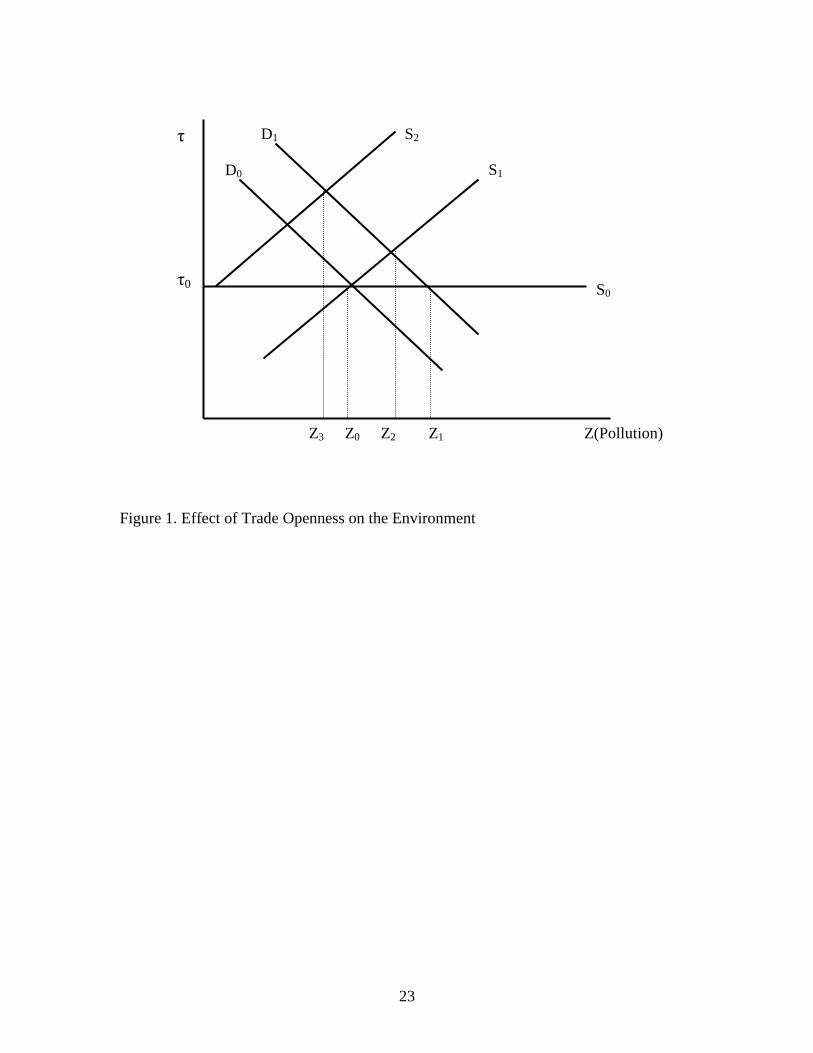
Following Copeland (2005), a simple model involving demand and supply of emissions

is presented in Figure 1 to examine the effects of trade liberalization on income and the

environment. In this model, a country is assumed to export pollution-intensive goods

(dirty goods) and a pollution tax ( ) is used as a proxy for the stringency of

environmental policy. The demand for emissions ( D ) is a derived demand, reflecting

emission of pollution as a side effect of production; a country produces more pollution as

a pollution tax (costs of environmental damage) is low. The supply of emissions ( S )

represents the country’s willingness to allow emissions as reflected by the pollution

policy.

Consider a country that has a fixed pollution tax. The supply curve is then 0S .

Initially equilibrium values for pollution tax ( 0 ) and pollution level ( 0Z ) are determined

by the intersection between the demand ( 0D ) and supply curves ( 0S ). In this case, trade

liberalization leads to an increase in exports of pollution-intensive goods and results in a

shift in the demand for emissions to 1D , thereby increasing in emissions to 1Z . On the

other hand, consider a situation where the government tightens up environmental policy

as pollution increases. The supply curve is then represented by 1S . In this case, a trade-

induced outward shift of demand for emissions leads to pollution at 2Z . As a result, the

endogenous policy response dampens the increase in pollution from 1Z to 2Z .

It should be emphasized that since the motivation for trade liberalization is

usually to increase real income in a country, income effects play a key role in the

analyses of trade effects on the environment (Copeland 2005). Figure 1 also can be used

to illustrate how income effects influence the predicted effects of trade and the

8

environment. Assume that the supply curve of emissions is income-responsive. In this

case, since environmental quality is a normal good, trade-induced income growth causes

people to increase their demand for a clean environment and results in a shift in the

supply of emissions to 2S if the government responses to people’s preference, which leads

to a decrease in pollution ( 3Z ) from trade liberalization despite the country having a

comparative advantage in the dirty goods. The magnitudes by which the supply curve

shifts back depend on income and substitution effects.

EMPRICIAL METHODOLOGY

This study examines the dynamic relationship between income, trade liberalization and

environmental quality for each of 50 developing and developed countries. There are two

emission variables that have been widely used in the literature: sulfur dioxide (SO2) and

carbon dioxide (CO2). Of these, SO2 represents the measure of local air pollution,

whereas CO2 represents a global pollutant (externality), which individual countries are

unable to regulate without international cooperation (Dinda 2004, Frankel and Rose

2005). It is thus more appropriate to use SO2 as a proxy for the measure of environmental

quality in our individual country-specific analysis.

Development of Empirical Time-Series Models

To examine dynamic interrelationship between trade, income and environmental quality

(SO2), the cointegrated vector autoregression (CVAR) model developed by Johansen is

applied (Johansen 1995). The Johansen method uses a statistical model involving up to k

lags as follows:

9

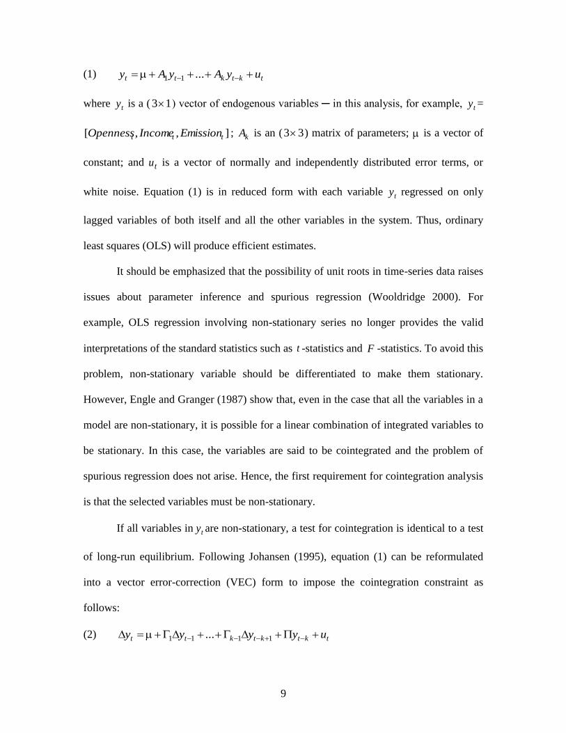
(1) 11 ... tktktt uyAyAy

where ty is a ( 13 ) vector of endogenous variables ─ in this analysis, for example, ty =

],,[ ttt EmissionIncomeOpenness ; kA is an ( 33 ) matrix of parameters; is a vector of

constant; and tu is a vector of normally and independently distributed error terms, or

white noise. Equation (1) is in reduced form with each variable ty regressed on only

lagged variables of both itself and all the other variables in the system. Thus, ordinary

least squares (OLS) will produce efficient estimates.

It should be emphasized that the possibility of unit roots in time-series data raises

issues about parameter inference and spurious regression (Wooldridge 2000). For

example, OLS regression involving non-stationary series no longer provides the valid

interpretations of the standard statistics such as t -statistics and F -statistics. To avoid this

problem, non-stationary variable should be differentiated to make them stationary.

However, Engle and Granger (1987) show that, even in the case that all the variables in a

model are non-stationary, it is possible for a linear combination of integrated variables to

be stationary. In this case, the variables are said to be cointegrated and the problem of

spurious regression does not arise. Hence, the first requirement for cointegration analysis

is that the selected variables must be non-stationary.

If all variables in ty are non-stationary, a test for cointegration is identical to a test

of long-run equilibrium. Following Johansen (1995), equation (1) can be reformulated

into a vector error-correction (VEC) form to impose the cointegration constraint as

follows:

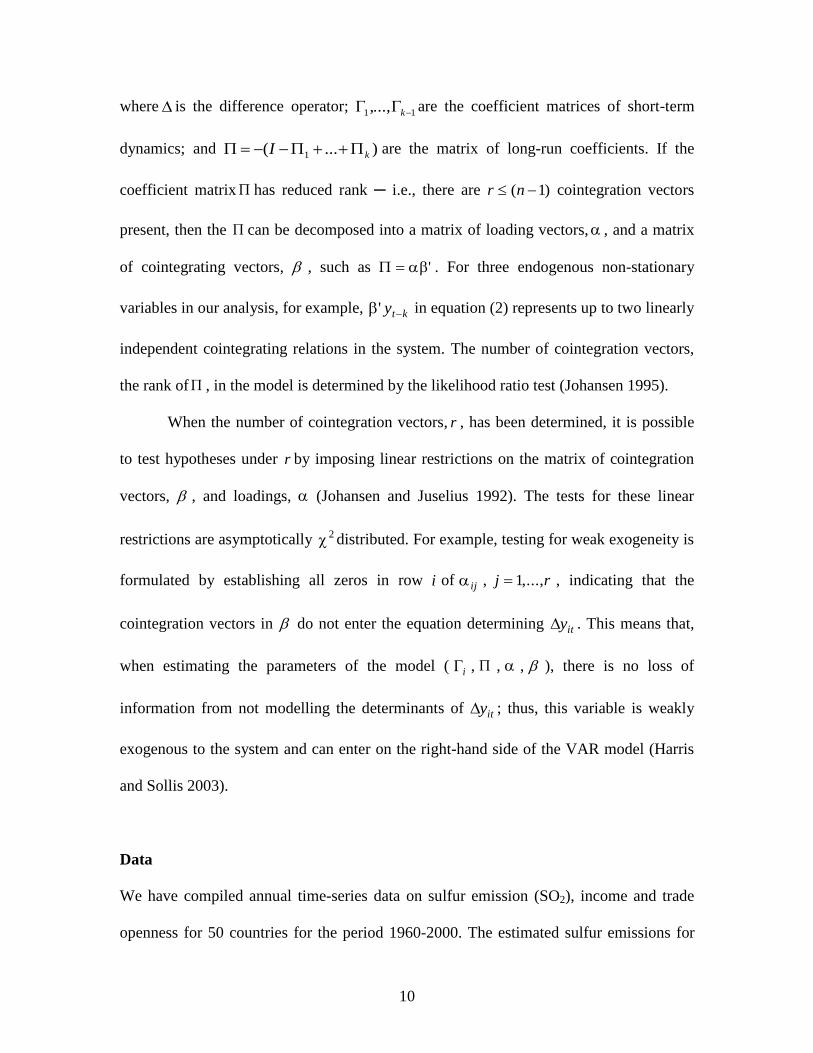
(2) tktktktt uyyyy 1111 ...

10

where is the difference operator; 11,..., kare the coefficient matrices of short-term

dynamics; and )...( 1 kI are the matrix of long-run coefficients. If the

coefficient matrix has reduced rank ─ i.e., there are )1( nr cointegration vectors

present, then the can be decomposed into a matrix of loading vectors, , and a matrix

of cointegrating vectors, , such as ' . For three endogenous non-stationary

variables in our analysis, for example, kty ' in equation (2) represents up to two linearly

independent cointegrating relations in the system. The number of cointegration vectors,

the rank of , in the model is determined by the likelihood ratio test (Johansen 1995).

When the number of cointegration vectors, r , has been determined, it is possible

to test hypotheses under r by imposing linear restrictions on the matrix of cointegration

vectors, , and loadings, (Johansen and Juselius 1992). The tests for these linear

restrictions are asymptotically 2 distributed. For example, testing for weak exogeneity is

formulated by establishing all zeros in row i of ij , rj ,...,1 , indicating that the

cointegration vectors in do not enter the equation determining ity . This means that,

when estimating the parameters of the model ( i , , , ), there is no loss of

information from not modelling the determinants of ity ; thus, this variable is weakly

exogenous to the system and can enter on the right-hand side of the VAR model (Harris

and Sollis 2003).

Data

We have compiled annual time-series data on sulfur emission (SO2), income and trade

openness for 50 countries for the period 1960-2000. The estimated sulfur emissions for

11

50 countries are obtained from a large database constructed by David Stern (Stern 2005

and 2006), which is known as the David Stern’s Datasite (available at the web site

http://www.rpi.edu/~sternd/datasite.html). To ensure comparability with per capita GDP

in the model, per capita SO2 emissions for individual countries (measured in kg) are

calculated using their population sizes. The per capita GDP (measured in real PPP-

adjusted dollars) is used as a proxy for income and is taken from the Penn World Table

(PWT 6.2) (available at the web site

http://pwt.econ.upenn.edu/php_site/pwt62/pwt62_form.php). The degree of openness of

an economy (defined as the ratio of the value of total trade to GDP) is used as a proxy for

trade openness and is obtained from the Penn World Table.

It should be pointed out that the data on sulfur emissions (SO2) used in empirical

studies have almost invariably come from a single source, the ASL and Associates

database (ASL and Associate 1997, Lefohn et al. 1999), which compiles annual time-

series data on SO2 for individual countries from 1850 to 1990. However, the

unavailability of data after 1990 has been an impediment to continued use of these

estimates for further research. Hence, David Stern has developed global and individual

country estimates of sulfur emissions from 1991 to 2000 or 2002 (most OECD countries)

combined with estimates from existing published and reported sources for 1850-1990

(see Stern (2005) for more details). In addition, following the World Bank’s country

classification, 50 countries used in our analysis are divided into two groups on the basis

of 2005 gross national income per capita: (1) 25 developing economies, $876- $10,725;

and (2) 25 developed economies, $10,726 or more.

12

Econometric Procedure

As noted earlier, the first requirement for the use of the Johansen cointegration

method is that the variables must be non-stationary. The presence of a unit root in ty (

ttt EmissionIncomeOpenness ,, ) for 50 countries is tested using the Dickey-Fuller

generalized least squares (DF-GLS) test (Elliot et al. 1996). This test optimizes the power

of the conventional augmented Dickey-Fuller (ADF) test by detrending. The DF-GLS test

works well in small samples and has substantially improved power when an unknown

mean or trend is present (Elliot et al. 1996). The results show that the levels of all the

series (150 series) are non-stationary, while the first differences are stationary. From

these findings, we conclude that all the series are non-stationary and integrated of order 1,

or )1(I ; therefore, cointegration analysis can be pursued on them.

It should be noted that, before implementing the cointegration test, the important

specification issue to be addressed is the determination of the lag length for the VAR

model, because the Johansen procedure is quite sensitive to changes in lag structure

(Maddala and Kim 1998). The lag length ( k ) of the VAR model is determined based on

the likelihood ratio (LR) tests. This method compares the models of different lag lengths

sequentially to see if there is a significant difference in results (Doornik and Hendry

1994). Of the 50 countries, for example, the hypothesis that there is no significant

difference between a two- and a three-lag model cannot be rejected for 19 countries. Thus,

two lags ( k =2) are used for those countries in our cointegration analysis. Diagnostic tests

on the residuals of each equation and corresponding vector test statistics support the VAR

model with two lags as a sufficient description of the data. In the residual serial

correlation and heteroskedasticity tests, the null hypotheses of no serial correlation and

13

no heteroskedasticity cannot be rejected at the 5% significance level. Although the null

hypothesis of normality is rejected for some cases at the 5% significance level, non-

normality of residuals does not bias the results of the cointegration estimation (Gonzalo

1994). For the remaining 31 countries, on the other hand, both the VAR lag selection

criterion and diagnostic tests consistently support k =1 as the most appropriate lag length

for the VAR model.3

EMPIRICAL RESULTS

With the selected lag lengths ( k =1 or k =2) in non-stationary VAR models, the Johansen

cointegration procedure is used to determine the number of cointegrating vectors among

the variables. The results indicate that one cointegration vector is found for 24 countries

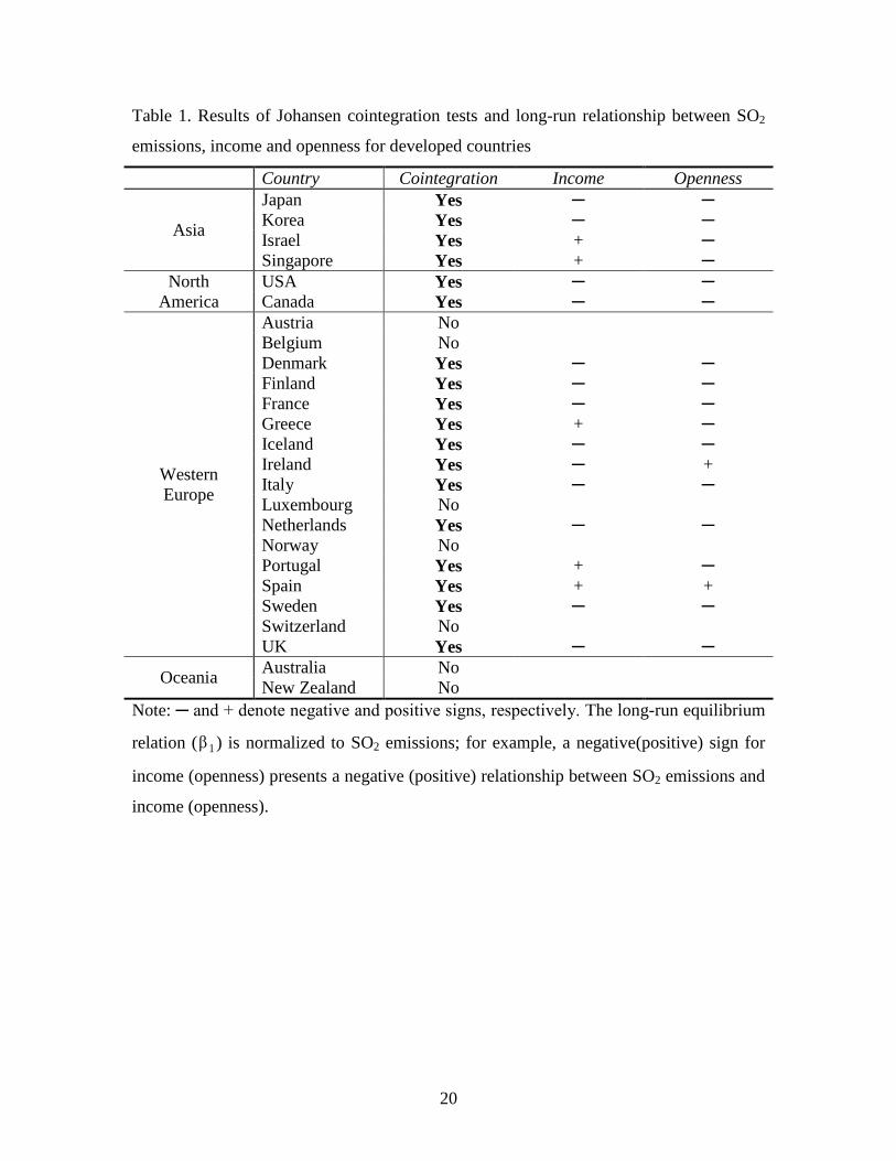
at the 5% significance level, whereas no cointegration is found for 26 countries (Tables

1-2). More specifically, of the 25 developed countries, the trace tests show that the

hypothesis of no cointegration ( r =0) is rejected and that of one cointegration vector ( r

=1) is accepted at the 5% level for 17 countries.4 For the remaining 8 countries, on the

other hand, the trace statistics are well below the critical value and r =0 cannot be

rejected at the 5% level, indicating that the three variables are not cointegrated. The

results thus, by and large, support for the hypothesis that cointegration between SO2

emissions, income and openness is pervasive across developed countries. In contrast, of

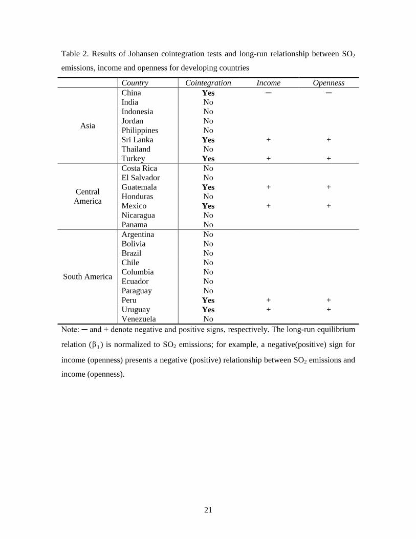
the 25 developing countries, the trace tests show that only 7 countries have a

cointegration rank of one ( r =1), while the remaining 18 countries have r =0. This

3 The results of unit roots and diagnostic tests are not reported here for brevity.

4 Interested readers can contact the authors for more details of cointegration test results.

.

14

finding indicates that the three variables have no inherent co-movement tendency over

the long-run across developing countries.

When determining the existence of cointegration relationship, the cointegration

vectors ( j ) estimated from equation (2) represent the long-run relationship among the

selected variables. More specifically, having obtained only one cointegration relationship

between SO2 emissions, income and openness in the 24 countries that include developed

and developing economies, the first eigenvector ( 1 ) of the three eigenvectors is most

highly correlated with the stationary part of the process ty when corrected for the lagged

values of the differences. Thus, 1 represents the cointegration vector determined by the

CVAR model (Johansen 1995). After normalizing the coefficient of SO2 emissions, for

example, the long-run equilibrium relation ( 1 ) between the three variables in the United

States can be represented as the following reduced form;

ttt OpennessIncomeEmmision 11.098.0 . In this equation, a negative coefficient of

income on sulfur emissions suggests that environmental quality improves as the U.S.

income increases. A negative coefficient of openness on SO2, on the other hand, implies

that trade liberalization tends to reduce SO2 emissions in the United States. Note that in

this study we do not interpret the coefficients of the long-run relationship as long-run

elasticities because such an interpretation may ignore the dynamics of the system

(Lütkepohl 2005). For example, a 1% increase in the U.S. real income may not cause a

long-term decline in SO2 emissions by 0.98% because an increase in the U.S. income is

likely to have an effect on trade openness as well that may interact in the long-run.

Analyzing Long-Run Relationship

15

As noted earlier, the cointegration vector, 1 , estimated from equation (2) is used to

describe the long-run relationship between SO2 emissions, income and openness after

normalizing the coefficients of SO2 emissions, and rearranging in reduced forms (Table

1). The results show that, of the 17 developed countries in which all three variables are

cointegrated, 12 countries show a negative long-run relationship between SO2 emissions

and per capita income, suggesting that pollution levels tend to decrease as a country’s

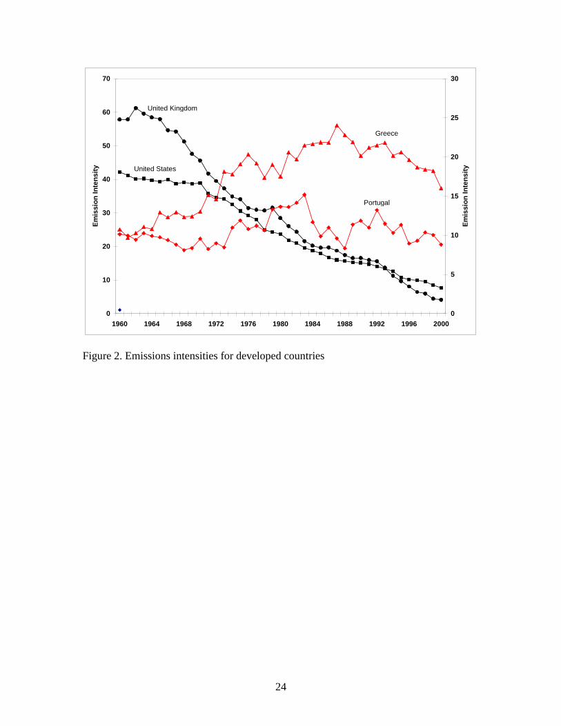
economy grows. For the remaining 5 countries (Israel, Singapore, Greece, Portugal and

Spain), on the other hand, SO2 emissions have a positive long-run relationship with per

capita income, indicating economic growth tends to worsen environmental quality. This

phenomenon could be directly associated with changes in emissions intensity. More

specifically, emissions intensity is defined as the ratio of sulfur dioxide emissions to a

measure of economic output (per capita income). Deterioration (improvement) of

emissions intensity implies that SO2 emissions tend to increase (decrease) as income

grows, which in turn indicates a positive (negative) relationship between SO2 emissions

and income.5 In fact, the emissions intensities of the 12 economies that show a negative

emission-income relationship have significantly improved over the last 50 years. In

contrast, the emissions intensities of the 5 economies that show a positive emission-

income relationship have improved little (Israel, Singapore and Spain) or even have

deteriorated (Greece and Portugal) over the last 50 years (Figure 2). In addition, of the 17

developed countries in which the three variables are cointegrated, 15 countries show a

negative long-run relationship between SO2 emissions and openness, indicating that air

pollution tends to decrease as a country’s exposure to international markets increases.

5 It should be noted that SO2 emissions can keep increasing unless emissions intensity improves faster than

the economy grows. In this case, SO2 emissions could have a positive relationship with income despite

improvement of emissions intensity.

16

These results support for the so-called gains-from-trade hypothesis for developed

countries; a rise in income growth through trade gradually tends to increase cleaner

techniques of production, thereby improving environmental quality.

On the other hand, of the 7 developing countries in which all three variables are

cointegrated, 6 countries (Peru, Uruguay, Guatemala, Mexico, Sri Lanka and Turkey)

show a positive long-run relationship between SO2 emissions and income, indicating that

economic growth worsens environmental quality (Table 2). In addition, in these 6

countries, SO2 emissions have a positive long-run relationship with openness, supporting

for the so-called race-to-the bottom hypothesis for developing countries; confronted with

international competition, poor open economies have incentives to adopt excessively lax

environmental standards in an effort to attract multinational corporations and export

pollution-intensive goods. As a result, trade is the cause of environmental degradation in

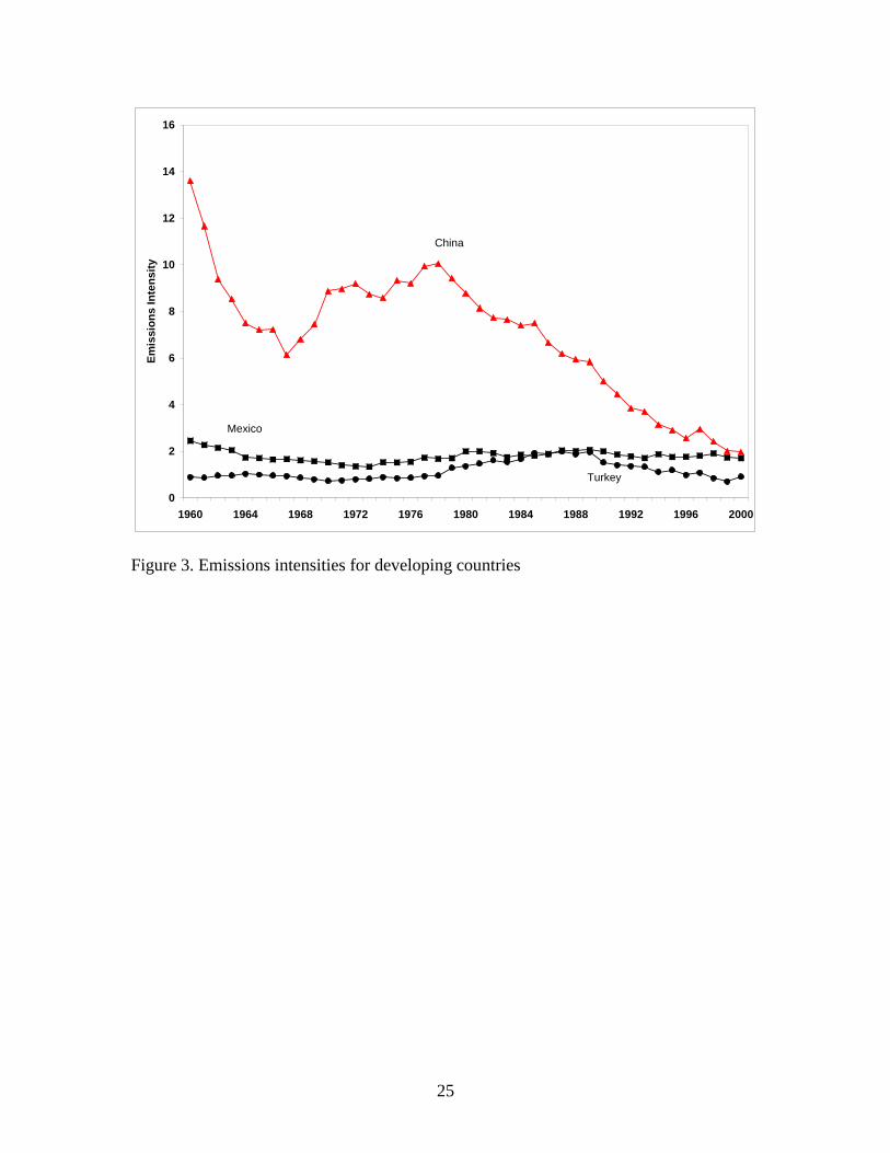
developing countries. For China, on the other hand, SO2 emissions have a negative long-

run relationship with income and openness, suggesting that growth and trade

liberalization improve environmental quality. In fact, unlike other developing countries,

the emissions intensity of the Chinese economy has substantially improved since 1978

(Figure 3). From these findings, therefore, it seems reasonable for us to conclude that,

among developing countries, only China has led to both continued economic growths

through more open trade and a cleaner environment.

Identifying the Causal Effects

In order to identify the casual effects of trade and income on the environment, the long-

run weak exogeneity test is conducted by restricting parameter in speed-of-adjustment

17

( ) to zero in the model. This test examines the absence of long-run levels of feedback

due to exogeneity (Johansen and Juselius 1992). In other words, a weakly exogenous

variable is a driving variable, which pushes the other variables adjusting to long-run

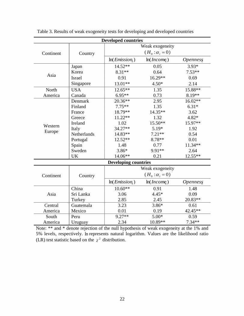
equilibrium, but is not influenced by the other variables in the model. The results show

that, of the 17 developed countries, the null hypothesis of weak exogeneity cannot be

rejected for openness and/or income at the 5% level for 14 countries (Table 3), indicating

that these two variables are weakly exogenous to the long-run relationships in the model.

For the remaining 3 countries, on the other hand, the null hypothesis cannot be rejected

for SO2 emissions. These findings indicate that, for developed countries, openness and/or

income are generally the driving variables in the system and significantly affect SO2

emissions in the long-run, but are not influenced by SO2 emissions. This implies that

trade liberalization and income growth may cause people in developed countries to

increase their demand for a cleaner environment, thereby enforcing strict environmental

regulations. This further suggests that the developed countries tend to restrain their

aspirations for income growth and/or freer trade in order to control environmental

degradation.

Of the 7 developing countries, on the other hand, the null hypothesis of weak

exogeneity cannot be rejected for SO2 emissions at the 5% level for 5 countries. For the

remaining two countries (Peru and China), on the other hand, the null hypothesis cannot

be rejected at the 5% level for openness and income, respectively. These results indicate

that, for developing countries, the SO2 emissions are generally weakly exogenous to the

long-run parameters in the system; thus, the emission does not adjust to deviations from

any equilibrium state defined by the cointegration relation. This suggests that trade

18

liberalization tends to create an incentive for pollution-intensive industries (so called

dirty industries) to relocate in developing countries with lower environmental standards

as developed countries adopt tighter environmental protection, thereby deteriorating

environmental quality. This further implies that that, if developing countries attempt to

control the emission rate, there will be a corresponding reduction in the income growth

rate and/or trade volume. As such, the developing countries may have to accept a

reduction of their current income levels and/or degree of trade openness if they have to

reduce permanently the emission level from what it is at present.

CONCLUSIONS

In this paper, we examine the long-run effect of trade liberalization on the environment

for both developing and developed countries over the last half-century. For this purpose,

the effects of the trade openness and per capita income on per capita SO2 emissions are

investigated using the Johansen multivariate cointegration analysis. It is generally found a

negative long-run relationship between SO2 emissions and income for developed

countries and a positive long-run relationship between them for developing countries. On

the other hand, we find that, while trade liberalization appears to increase environmental

quality in developed economies, it has a detrimental effect on environmental quality in

most developing countries. We also find that for developed countries the causality seems

to run from trade and/or income to SO2 emissions. For developing countries, on the other

hand, the causality is found to run in the opposite direction from SO2 emissions to trade

and/or income. These results imply that for developed economies SO2 emissions are the

19

adjusting parts, while trade/income are the determining parts of the long-run relationship,

and the opposite relationship holds for developing countries.

20

Table 1. Results of Johansen cointegration tests and long-run relationship between SO2

emissions, income and openness for developed countries

Country Cointegration Income Openness

Asia

Japan Yes ─ ─

Korea Yes ─ ─

Israel Yes + ─

Singapore Yes + ─

North

America

USA Yes ─ ─

Canada Yes ─ ─

Western

Europe

Austria No

Belgium No

Denmark Yes ─ ─

Finland Yes ─ ─

France Yes ─ ─

Greece Yes + ─

Iceland Yes ─ ─

Ireland Yes ─ +

Italy Yes ─ ─

Luxembourg No

Netherlands Yes ─ ─

Norway No

Portugal Yes + ─

Spain Yes + +

Sweden Yes ─ ─

Switzerland No

UK Yes ─ ─

Oceania Australia No

New Zealand No

Note: ─ and + denote negative and positive signs, respectively. The long-run equilibrium

relation ( 1 ) is normalized to SO2 emissions; for example, a negative(positive) sign for

income (openness) presents a negative (positive) relationship between SO2 emissions and

income (openness).

21

Table 2. Results of Johansen cointegration tests and long-run relationship between SO2

emissions, income and openness for developing countries

Country Cointegration Income Openness

Asia

China Yes ─ ─

India No

Indonesia No

Jordan No

Philippines No

Sri Lanka Yes + +

Thailand No

Turkey Yes + +

Central

America

Costa Rica No

El Salvador No

Guatemala Yes + +

Honduras No

Mexico Yes + +

Nicaragua No

Panama No

South America

Argentina No

Bolivia No

Brazil No

Chile No

Columbia No

Ecuador No

Paraguay No

Peru Yes + +

Uruguay Yes + +

Venezuela No

Note: ─ and + denote negative and positive signs, respectively. The long-run equilibrium

relation ( 1 ) is normalized to SO2 emissions; for example, a negative(positive) sign for

income (openness) presents a negative (positive) relationship between SO2 emissions and

income (openness).

22

Table 3. Results of weak exogeneity tests for developing and developed countries

Developed countries

Continent Country

Weak exogeneity

( 0:0 iH )

)ln( tEmission )ln( tIncome tOpenness

Asia

Japan 14.52** 0.05 3.93*

Korea 8.31** 0.64 7.53**

Israel 0.91 16.29** 0.69

Singapore 13.01** 4.50* 2.14

North

America

USA 12.65** 1.35 15.88**

Canada 6.95** 0.73 8.19**

Western

Europe

Denmark 20.36** 2.95 16.02**

Finland 7.75** 1.35 6.31*

France 18.79** 14.35** 3.62

Greece 11.22** 1.32 4.82*

Ireland 1.02 15.50** 15.97**

Italy 34.27** 5.19* 1.92

Netherlands 14.83** 7.21** 0.54

Portugal 12.52** 8.78** 0.01

Spain 1.48 0.77 11.34**

Sweden 3.86* 9.91** 2.64

UK 14.06** 0.21 12.55**

Developing countries

Continent Country

Weak exogeneity

( 0:0 iH )

)ln( tEmission )ln( tIncome tOpenness

Asia

China 10.60** 0.91 1.48

Sri Lanka 3.06 4.45* 0.09

Turkey 2.85 2.45 20.83**

Central

America

Guatemala 3.23 3.86* 0.61

Mexico 0.01 0.19 42.45**

South

America

Peru 9.27** 5.00* 0.59

Uruguay 2.34 10.89** 7.34**

Note: ** and * denote rejection of the null hypothesis of weak exogeneity at the 1% and

5% levels, respectively. ln represents natural logarithm. Values are the likelihood ratio

(LR) test statistic based on the 2 distribution.

23

Figure 1. Effect of Trade Openness on the Environment

S0

S1

S2

Z3 Z0 Z2 Z1 Z(Pollution)

τ0

τ

D0

D1

24

Figure 2. Emissions intensities for developed countries

0

10

20

30

40

50

60

70

1960 1964 1968 1972 1976 1980 1984 1988 1992 1996 2000

Em

iss

ion

In

ten

sit

y

0

5

10

15

20

25

30

Em

iss

ion

In

ten

sit

yUnited States

United Kingdom

Greece

Portugal

25

Figure 3. Emissions intensities for developing countries

0

2

4

6

8

10

12

14

16

1960 1964 1968 1972 1976 1980 1984 1988 1992 1996 2000

Em

iss

ion

s I

nte

ns

ity

Mexico

Turkey

China

26

REFERENCES

ASL and Associates. 1997. Sulfur emissions by country and year. Report No:

DE96014790. U.S. Department of Energy, Washington, DC.

Chintrakarn, P., and Millimet, D.L. 2006. The environmental consequences of trade:

evidence from subnational trade flows. Journal of Environmental Economics and

Management 52(1): 430-453.

Coondoo, D., and Dinda, S. 2002. Causality between income and emission: a country

group-specific econometric analysis. Ecological Economics 40(3): 351-367.

Copeland, B.R., and Taylor, M.S. 1994. North-South trade and the environment.

Quarterly Journal of Economics 109(3): 755-787.

Copeland, B.R., and Taylor, M.S. 2004. Trade, growth, and the environment. Journal of

Economic Literature 42(1): 7-71.

Copeland, B.R. 2005. Policy endogeneity and the effects of trade on the environment.

Agricultural and Resource Economics Review 34(1): 1-15.

Dean, J. 2002. Does trade liberalization harm the environment? A new test. Canadian

Journal of Economics 35(4): 819-842.

Dinda, S. 2004. Environmental Kuznets curve hypothesis: a survey. Ecological

Economics 49(4): 431-455.

Dinda, S., and Coondoo, D. 2006. Income and emission: a panel data-based cointegration

analysis. Ecological Economics 57(2): 167-181.

Doornik, J., and Hendry, D. 1994. Interactive econometric modeling of dynamic System

(PcFiml 8.0). London: International Thomson Publishing.

27

Doornik, J., and Hendry, D. 2001. Empirical econometric modeling (PcGive 10).

Timberlake Consultants Ltd, London, UK.

Elliot, G., Rothenberg, T.J., and Stock, J.H. 1996. Efficient tests for an autoregressive

unit root. Econometrica 64(4): 813-836.

Engle, R., and Granger, C.W.J. 1987. Cointegration and error-correction: representation,

estimation and testing. Econometrica 55: 251-276.

Frankel, J.A., and Rose, A.K. 2005. Is trade good or bad for the environment? Sorting out

the causality. Review of Economics and Statistics 87(1): 85-91.

Gale, L.R., and Mendez, J.A. 1998. The empirical relationship between trade, growth and

the environment. International Review of Economics and Finance 7(1): 53-61.

Gonzalo, J. 1994. Five alternative methods of estimating long-run equilibrium

relationships. Journal of Econometrics 60(1-2): 203-233.

Grossman, G.M., and Krueger, A.B. 1991. Environmental impacts of the North American

Free Trade Agreement. NBER. Working paper 3914.

Grossman, G.M., and Krueger, A.B. 1993. Environmental impacts of the North American

Free Trade Agreement, in Peter Garber (Ed.), The U.S.-Mexico Free Trade

Agreement. MIT Press, Cambridge.

Harris, R., and Sollis, R. 2003. Applied time series modeling and forecasting. Chichester,

W. Sussex: John Wiley and Sons.

Johansen, S. 1995. Likelihood-based inference in cointegrated vector autoregressive

models. Oxford: Oxford University Press.

28

Johansen, S., and Juselius, K. 1992. Testing structural hypotheses in a multivariate

cointegration analysis of the PPP and the UIP for UK. Journal of Econometrics

53(1-3): 211-244.

Lefohn, A.S., Husar, J.D., and Husar, R.B. 1999. Estimating historical anthropogenic

global sulfur emission patterns for the period 1850-1990. Atmospheric

Environment 33(21): 3435-3444.

Lucas, R.E.B., David, W., and Hemamala, H. 1992. Economic development,

environmental regulation and the international migration of toxic industrial

pollution: 1960-1988, in Patrick Low (Ed.), International trade and the

environment. World Bank Discussion Paper No. 159. Washington DC: World

Bank, 1992, pp. 67-86.

Maddala, G.S., and Kim, I.M. 1998. Unit roots, cointegration, and structural change.

Cambridge: Cambridge University Press.

Perman, R., and Stern, D.I. 2003. Evidence from panel unit root and cointegration tests

that the environmental Kuznets Curve does not exist. Australian Journal of

Agricultural and Resource Economics 47(3): 325-347.

Porter, M., and van der Linde, C. 1995. Toward a new conception of the environment-

competitiveness relationship. Journal of Economic Perspectives 9(4): 97-118.

Sims, C. 1980. Macroeconomics and reality. Econometrica 48(1): 1-48.

Stern, D.I. 2005. Global sulfur emissions from 1850-2000. Chemosphere 58(2): 163-175.

Stern, D.I. 2006. Reversal of the trend in global anthropogenic sulfur emissions. Global

Environmental Change 16(2): 207-220.

29

Wooldridge, J.M. 2000. Introductory econometrics: a modern approach. Mason, Ohio:

South-Western College Publishing.