The ENIAC:

Then and Now

Brian L. Stuart

Drexel University

The ENIAC

1

What Is ENIAC?

• Large-scale computing system

• Contracted in 1943 for the US Army

• Built during WWII• Dedicated February 15, 1946

• Converted to sequential instruction execution in 1948

• Retired 1955

• Used for:

– Atomic bomb development

– Ballistics trajectories

– Number theory– Weather prediction

– and more

2

Key People

3

Common Statistics

• 40 racks, each 8’ by 2’

• About 18,000 tubes

• 100KHz basic clock

• 200µS addition time

• About 150KW of power

• 29 power supplies• 78 DC voltages

4

Basic Architecture

• Initiating unit• Cycling unit

• Two-panel master programmer

• 20 Accumulator units

• Multiplying unit

• Divider/Square rooter unit

• 3 Function table units• Constant transmitter/card reader unit

• Card punch unit

5

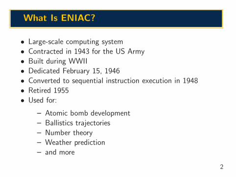
Moore School Layout

6

Unusual Characteristics

• No bulk writeable memory

• No separation between storage and computation

• Divider/square rooter not always exact

• Very parallel

This was a highly parallel machine, before vonNeumann spoiled it.— D.H. Lehmer

• Initially programmed with wires and switches

• Feels like a dataflow architecture

7

Cycling Unit

• Distributes multi-phase clock throughout system

• Oscilloscope for monitoring individual clock signals

• 100 KHz design rate

• 60 KHz for stability for sometime after move to Aberdeen

• Three clock modes:

– Continuous

– One add time– One pulse

8

Hand-Held Control

9

Clock Signals

10

Accumulator

• 10 digits + sign (P or M)

• Negative numbers stores as M + 10s complement

• 5 inputs: α, β, γ, δ, and ǫ

• 2 outputs: A and S

• 12 programs:

– Operation: α, β, γ, δ, ǫ, 0, A, AS, or S

– Clear/correct– Repeat count (on programs 5–12)

11

Decade Counter Module

12

Decade Counter Schematic

13

Reading From Accumulator

Carry10P

A S

9P

14

How it Works

• Add Accumulator 3 to Accumulator 4

• Accumulator 3 has 15 and Accumulator 4 has 27

• Control signal sent to both accumulators• Accumulator 3 program sends 1 pulse on 10s line and 5 pulseson 1s line

• Accumulator 4 program receives pulses from Accumulator 3:

– 10s digit advances to 3

– 1s digit advances to 2 with carry flipflop set

• Carry gate propagates carry, advancing 10s digit to 4

• Accumulators emit control pulse to trigger next operation

15

Setup

Accumulator Accumulator Accumulator3 4 5

AS β β

1 1 1

α α α

16

Simulator Specification

p a3.A 2

p a3.S 3

p 2 a4.beta

p 3 a5.beta

p 1-3 a3.5i

p 1-3 a4.5i

p 1-3 a5.5i

s a3.op5 AS

s a4.op5 beta

s a5.op5 beta

s cy.op 1a

17

Multiplier

• 3 racks

• p-digit multiplier

• Computes in p+ 4 addition times• Uses digit multiplication table

• Fixed connections to accumulators:

– Multiplier– Multiplicand

– Product

18

Multiplication Example

• 42 times 347

• 4× 347 = 1200 + 160 + 28

– Left-hand partial product: 1120000000– Right-hand partial product: 0268000000

• 2× 347 = 600 + 800 + 14

– Add to LHPP: 0001000000

– Add to RHPP: 0068400000

• LHPP: 1121000000, RHPP: 0336400000

• Add: 1457400000

19

Master Programmer

• 10 6-stage counters

• 20 decade counters

• Complex nested loop structures

• Negative/non-negative conditional branching:

– Accumulator output sign into dummy program

– Dummy program output into stage direct input

– Two stage program outputs trigger negative and non-negative actions

• “Computed goto:”

– Run selected digit output into stage direct input

– Stages 1–6 program outputs trigger actions based on val-ues 0–5 of accumulator digit

20

Setup

Master-Programmer

Accumulator Accumulator Accumulator1 2 3

α

1

β

1

A

1

0

1

α

1

α

1

α A A

0

1

α S A

S(sign)

Acc1A

3

A

2

2

×

21

Simulator Specification

p 1 a1.a

p 1 a1.b

p a2.A 1

p a3.A 1

p a3.S 1

p a1.A ad.dp.1.11

p ad.dp.1.11 a2.5i

p 1-3 a1.5i

p 1-3 a2.2i

p a1.5o 1-4

p 1-4 a1.6i

p 1-4 a3.2i

p a1.6o 1-5

p 1-5 a1.7i

p a2.5o 1-6

p 1-6 p.Adi

p a1.7o a1.8i

p a1.8o 1-7

p 1-7 p.Ai

p p.A1o 1-8

p p.A2o 1-9

p 1-8 a1.9i

p 1-9 a1.10i

p 1-8 a2.3i

p 1-9 a3.3i

s a1.op5 a

s a1.rp5 1

s a1.cc5 0

s a1.op6 b

s a1.rp6 1

s a1.cc6 0

s a1.op7 A

s a1.rp7 1

s a1.cc7 C

s a1.op8 0

s a1.rp8 1

s a1.cc8 0

s a1.op9 a

s a1.rp9 1

s a1.cc9 0

s a1.op10 a

s a1.rp10 1

s a2.op2 A

s a2.cc2 0

s a2.op3 A

s a2.cc3 0

s a2.op5 0

s a2.rp5 1

s a2.cc5 0

s a3.op2 S

s a3.cc2 0

s a3.op3 A

s a3.cc3 0

s p.a20 A

s p.d20s1 2

s p.d20s2 2

s p.cA 3

22

Programming

• Pre April 1948

– Unit operations selected by panel switches– Sequencing:

∗ Switch settings on master programmer

∗ Cables carrying programming pulses

• Post April 1948

– “Programming” to implement instruction set processor

– Instructions stored on portable function tables– Multiple instruction set proposals:

∗ 51-code design: uses only original ENIAC hardware

∗ 60-code design: uses new converter unit

∗ 94-code design: uses new converter unit

23

Memory Enhancement

• Early suggestion of accumulators without arithmetic

• Proposal for delay line register to be supplied by EMCC

• 100 word core memory module in 1953 supplied by Burroughs

24

Simulation Techniques

• Graphics

– Picture fragments cut from period and recent photographs

– Reconstructed unit pictures

– Ray tracing with synthetic geometry

• GUI using TCL/Tk application wish

• Pulse simulation

– Program pulses by single Go channel messages

– Data trunk pulses in parallel with integer channel mes-sages

– Acknowledgement messages

• http://cs.drexel.edu/~bls96/eniac/eniac.html

25

Simulator Examples

26

Questions?

27