The Emergence of a Major Invoicing Currency

Edwin L.-C. LAI�and Jing ZHOUy

Very Preliminary. Please do not circulate.September 20, 2012

Abstract

This paper proposes a model to explain how the currency of a country evolves in im-portance as an invoicing currency in trade settlement as the relative size of the countrygrows. The coalescing e¤ect, which induces individual �rms to choose the similar invoicingcurrency mix as their competitors so as to limit output volatility, not only facilitates theinternationalization of a currency, but also accelerates this process by creating a positivefeedback between actions of individual �rms and their competitors. We also show that,as the country grows, its currency is more likely to be used by small and close tradingpartners to invoice trade than its larger and less close counterparts. Moreover, wider use ofa currency for invoicing in the issuing country�s home market would help spread the use ofthe currency to other markets. Furthermore, we can explain the �tipping phenomenon��the non-linear relationship between the international use of a currency and the economicsize of the issuing country. The non-linearity arises from an a¢ nity for the establishedinternational currency. We confront our hypotheses with trade invoicing data on euro anddollar of 35 countries (1998-2010) and invoicing data on four major international curren-cies for trade between Thailand and 19 countries (2001-2008), and �nd that the results areconsistent with our theory.Keywords: currency, invoicing, vehicle currency, currency internationalization, pass-

through

�Hong Kong University of Science and Technology. Email: elai@ust.hk; edwin.l.lai@gmail.comyHong Kong University of Science and Technology. Email: jzhoubb@ust.hk

1

1 Introduction

This paper proposes a theory to explain how the currency of a country emerges as an interna-

tional currency in trade settlement and then confronts the theory with data. In principle, this

currency can be any currency. However, we do have in mind the Chinese renminbi (hereinafter

RMB) when we write the paper.

Interests in the potential of the RMB to become internationalized is fueled by the rise of

China, the mounting external debts of the US as well as the unresolved European debt crisis.

The RMB is currently not quali�ed as an international currency because China�s underdevel-

oped �nance impedes China to develop a thick market, a precondition for a currency to become

widely used. Nevertheless, as is well known, China also enjoys exceptional advantages in mak-

ing its currency internationalized: as the second largest economy in the world, it has the scale

necessary in order to create deep and liquid markets. The sheer volumes of its foreign trade

and inward foreign direct investment create a large installed base for RMB-based transactions.

Besides, since the eruption of the global economic crisis in 2008-2009, the supreme position of

the U.S. dollar as a global medium of exchange and a reserve currency is eroded; by contrast,

China�s continuing robust growth in the last three decades inspires worldwide con�dence in

China as a growth engine capable of leading the recovery of the global economy. Therefore,

the RMB has great potential to become internationalized in the sense that a global role of

currency should be commensurate with its home country�s huge economic might in the long

run, as indicated by many previous studies on internationalization of currencies (e.g. Krugman

1984, Eichengreen 2011).

However, a more important question for Chinese and other countries�policy makers is: how

would the dynamic course of the internationalization look like, assuming China can keep its

current growth and the Chinese authorities set their minds to overcome their disadvantages

step by step? Looking back at the history of the replacement of the sterling by the U.S. dollar,

the most noticeable pattern may be a slow pace of increase in the adoption of the new currency

in international trade invoicing, followed by a sharp rise later. The dollar in 1914, like the

RMB today, played a negligible role in the world, although the United States was the largest

trading nation by then. In the years after the First World War, this trend continues with

sterling playing an important role in global trade settlement, despite the decline of Britain as

a global economic power. However, a dramatic change follows: after the Second World War

1

the collapse of sterling accelerated and the dollar replace sterling as the leading international

currency.

The above paragraph describes how one currency (the US dollar) evolved to become a

dominant reserve currency over time. It was observed that the time trajectory of the reserve

share of the currency was highly non-linear with respect to the economic size of the country

as the country�s share of global GDP grew. Interestingly, when comparing across countries

at any given time, we also observe such non-linearity. That is, when examining the reserve

shares of the �ve major international currencies in the world nowadays � the U.S. dollar, the

euro, the British pound sterling, the Japanese yen and the Swiss franc � we observe that the

responsiveness of reserve share of a currency to changes in the determinant variables (such as

global GDP share of the country) is much smaller when the reserve share is low than that when

the reserve share is high. Consequently, the top reserve currency attains a disproportionately

high reserve share relative to its GDP share. This convex relationship between the share of

a country�s currency in central banks� reserves and its economic size is called the �tipping

phenomenon�.

Krugman (1984) suggests a non-linear curve that depicts the relationship between the de-

sired use of an international currency and its actual use. The desired use of a currency increases

in its actual use, with the slope increasing when the actual use is low and decreasing when the

actual use is high. This relationship would be very helpful for investigating the course of RMB�s

global use as an invoicing currency if we can understand the underlying rationale, which, un-

fortunately, is not provided by Krugman�s paper.

As we review the literature, we found that there is a shortage of theories that explain the

process of internationalization of a currency, in sharp contrast to the relatively richer body

of empirical studies. Matsuyama et al (2001) and Rey (2001) are two notable exceptions.

Matsuyama et al (2001) use the framework of random matching games to discuss whether

and how a national currency become circulated internationally under di¤erent scenarios in a

two-country model. They also point out that the use of money as medium of exchange hinges

critically on a strategic externality and economies of scale and therefore the currency of a larger

country has higher chance to be accepted as an international currency. Rey (2001) seeks to

explain the rise and fall of the pound and the dollar as vehicle currencies with a cash-in-advance

model in an open economy framework where explicit transaction technology is added.

The common focal point of both papers is the lubricating function of a currency, i.e. the

2

medium of exchange to lower transaction costs. However, this may not be the most important

factors, at least not the only one, to determine how internationalized a currency can go, as

indicated by Goldberg and Tille (2008). They show with quantitative results both from model

and empirical tests that transaction cost is a much minor factor compared to the �coalescing

e¤ect�which means �rms are motivated to follow the invoicing currency choice of its competi-

tors in the market to minimize their price volatilities relative to others. This e¤ect plays an

essential role in limiting the �uctuations of pro�t �ows of a �rm, especially when prices are not

adjusted frequently.

The goal of this paper is to construct a theory to explain how a country�s currency becomes

more heavily used as an invoicing currency as the country�s economic size increases, and then

test the theory. In particular, we extend the model of Goldberg and Tille (2008) to a model

with multiple countries and multiple currencies. The main intuition is that �rms would like to

coalesce to use the mainstream currency in the market to invoice and settle to minimize their

price volatility relative to the market. When one of its foreign markets has grown, exporters

have to put more weight on the price index of this market and have to invoice a higher fraction

of their exports to this market in the local currency. When every �rm chooses to do so, the

invoicing share of this currency in markets other than this market would also rise accordingly

so as to limit goods arbitrage.

Furthermore, as a market grows relative to the rest of the world, �rms from di¤erent

countries adjust the compositions of their invoicing currencies at di¤erent paces: �rms in

small and nearby trading partners, which usually have smaller domestic markets and rely more

heavily on selling to this growing market, are more sensitive to the change, and they adjust

the compositions of their invoicing currency faster than their counterparts in larger trading

partners. Thus, there is larger impact of the growing market on smaller and nearer countries.

The above two paragraphs describe two channels a¤ecting the increasing use of a currency in

trade invoicing: one is the direct channel which means the home country�s larger size implies the

home country�s higher share in the sales of exporters and hence the higher share of its currency

being used abroad; the other is the indirect channel, which is the spillover of the currency use

from this growing market to other markets. These two channels will both contribute to the

�tipping phenomenon�: the impact of the direct channel is relatively weak when the rising

country is still small due to the dilution of trade costs. In addition, the self-justi�cation of

established vehicle currencies would be a bigger obstacle to the wide circulation of the new

3

vehicle currency when its home country is smaller. However, the direct e¤ect will get stronger

as the country grows relative to the rest of the world. The indirect channel also gets relatively

stronger when the country is larger because the strengthened direct channel widens the gap

between the use of its currency in its home market and in other markets. This wider gap implies

that each exporter has to adjust the composition of its invoicing currencies by a larger degree

for the same shift in the shares of markets in sales. Both channels give rise to an increasing

but convex relationship between the share of the global use of the currency and the world GDP

share of its home country.

We confront the theoretical implications with data on the use of euro and dollar as invoicing

currency in exports and imports in 35 countries (1998-2010) and data on the use of four major

international currencies � U.S. dollar, the euro, British pound sterling and Japanese yen in

Thailand�s trade (2001-2008). The empirical results are not only consistent with our theoretical

predictions, but also show the importance of the mechanisms we emphasize.

The remainder of the paper is organized as follows: Section 2 presents a model with multiple

countries and multiple currencies. We compare the choice of the composition of invoicing

currencies by �rms in countries of di¤erent sizes. Based on this analysis we compute the

trajectory of the global use of a currency as the issuing country grows relative to the rest of

the world. Section 3 tests the empirical implications of the model by confronting it with data

on invoicing currencies from di¤erent countries. Section 4 concludes the paper.

2 A Three-Country / Two-Market / Two-Currency Model ofInvoicing

This section develops a model of vehicle currency that is inspired by Goldberg and Tille (2008).

Our model has two major di¤erences from theirs: (i) �rms export to multiple markets; (ii) we

consider a Nash equilibrium where each exporter makes an optimal invoicing-currency decision

given the invoicing-currency decisions of all other exporters. We describe the environment in

section IIA and solve the model in section IIB. In section IIIC and IIID we discuss how a

currency becomes more widely used as a vehicle currency for trade settlement as the issuing

country grows relative to the rest of the world.

4

2.1 The Setup of the Model

We consider a world with three countries � a large country A, a growing country B and a

small country C. The sizes of country B and C are initially small relative to country A. And

the size of country B keeps growing while the sizes of country A and C remain unchanged. The

local currencies of the three countries are denoted by a, b and c respectively. We assume that

there is one single vehicle currency in the beginning, currency a, and we focus on the emergence

of currency b as another vehicle currency as country B grows. We always ignore the possibility

of currency c as a candidate for international currency due to C�s small size.

The markets in the world can be divided into two: market A0 and market B. Market A0 is

country A plus country C (and possibly other small countries whose size are also ignorable).

It is mainly dominated by a, at least when B does not dominate over A. In contrast, market

B is initially dominated by a but possibly occupied by b during B�s growth. An exporting

�rm�s owner needs to decide which currencies to invoice her products. Speci�cally, an exporter

in country E (E 2 fA;B;Cg), produces a brand z and sells it in the two markets. She postsher price P kE(z) in currency kE before knowing the realization of various shocks a¤ecting the

economy. The invoicing currency kE can be a basket of currency a and b, with a share of �E

on b (and therefore 1� �E on a). At the aggregate level, we assume that a share of �A0 of theaggregate price PA0 is invoiced in currency b in market A0 while a share of �B of the aggregate

price PB is invoiced in currency b in market B. We assume �B > �A0 and will show later that

it is true in equilibrium. The variables �E and �D (D 2 fA0; Bg) can be understood as thepartial pass-through of exchange rate to the price.1,2 E is the share of market B in the total

sales of a country-E �rm in steady state. Note that all variables �, , and � pertain to either

currency b or market B without explicitly indicating so.

Note that the price P kE(z) and the invoicing currency kE set by a �rm are applied to both

of its markets. And we assume that the invoicing currency is also the one actually used in the

payment.3 These assumptions eliminate the possibility of good arbitrage in principle.4

1From now on, we use E as a general notation for exporting countries and D for destination market. Also,we use e to denote the currency of the exporting country.

2This way to present a partial pass-through of exchange rate �uctuations to consumer prices is standard inliterature Corsetti and Pesenti (2005, 2002), Engel (2006), Goldberg and Tille (2008).

3Krugman (1984), Friberg and Wilander (2007)4 It can also be relaxed without hurting the essence of our model. If we assume that a �rm can invoice in

di¤erent currencies for di¤erent markets, say, in currency k1 and k2 for market A0 and B respectively, the pricesin the two markets will be practically di¤erent after the realization of exchange rates. Therefore, given thevolatility of the exchange rates, a �rm should make her baskets of k1 and k2 not deviate from each other too

5

Firms face monopolistic competition in both markets and the demand functions are:

YEA0 =

�SekETEA0P

kE

SeaPA0

���CA0 and YEB =

�SekETEBP

kE

SebPB

���CB

where PA0 and PB are the price indices across all brands on both markets denominated in their

local currencies; Sea is the exchange rate between currency e (the currency of the exporting

country) and currency a with an increase corresponding to a depreciation of currency e; CA0

and CB are the (exogenous) aggregate demands across all brands in market A0 and B; TEA0

and TEB capture a variety of exogenous trade frictions that can distort the prices faced by

consumers in the two markets. � > 1 is the price-elasticity of demand.

The meanings of the trade costs TEA0 and TEB here are richer than one might think. There

are at least two types of elements involved: One is the traditional trade costs. Countries di¤er

in trade costs due to transportation costs, trading bloc memberships or extents of economic

integration. This will make the breadth and depth of the circulation of a vehicle currency

substantially vary across countries. Another is factors that are associated with a currency�s

international role. Given prices and exchange rates, consumers prefer to use currencies that

are widely used.5 Wright and Trejos (2001) shows that a currency gains additional value if

it circulates abroad. Established vehicle currencies are also usually freely convertible at lower

transaction costs. These components of self-justi�cation and self-reinforcement are particularly

important to newly internationalized currencies.

We assume that T��AA0T�AB > T��CA0T

�CB > T��BA0T

�BB. It means that with normalized trade

costs in marketB, countryA is more advantageous than countryB in marketA0 while country C

is just in between. For convenience of presentation, we let T��EA0T�EB = TE , thus the assumption

becomes TA > TC > TB.

The technology for production is decreasing returns to scale with the degree of returns to

scale 0 < � < 1:

YE =1

�(HE)

�

where HE is a composite input with a unit cost of WE in her local currency.

far to limit the potential of arbitrage. An simply policy for a �rm is k2 = k1 + k0 where k0 is a constant whichre�ects the tolerance of the producer on its expected price di¤erence ex ante.

5Wright and Trejos (2001) shows that a currency gains additional value if it circulates abroad.

6

2.2 The invoicing-currency choice of a �rm

First we determine the invoicing currency choice of a typical �rm in each country. We deal

with the problem of an exporter from country C; those of �rms from countres A and B are

just analogous.

An exporter in C sets her price P kC in currency kC to maximize her discounted expected

pro�ts:6

maxPkC ;�C

�C = EdC [SckCPkC(YCA0 + YCB)�WC�

1� (YCA0 + YCB)

1� ]

= EdC

(SckCP

kC

"�SckCTCA0P

kC

ScaPA0

���CA0 +

�SckCTCBP

kC

ScbPB

���CB

#

�WC�1�

"�SckCTCA0P

kC

ScaPA0

���CA0 +

�SckCTCBP

kC

ScbPB

���CB

# 1�

9=;where dC is the state-speci�c discount factor which is independent of the pro�ts of a particular

�rm.

The maximization problem is di¢ cult to solve in general. We approximate the logarithm

of the pro�t function to second order around a steady state where the economy is not a¤ected

by any shock.7 In steady state the choice of invoicing currency would be irrelevant because all

currencies are equivalent to each other given that exchange rates are �xed. What matters is

only the pricing decision. With this independence, we can separate the maximization over P kC

and over �C and obtain the following solution for �C (refer to Appendix 5.1 for details):

�C = [(1� C)�A0 + C�B] + (1� )�C

where C is the share of market B in the total sales of a country-C �rm in steady state;

�C =E(mCsab)E(sab)2

+ E(sacsab)E(sab)2

where mC =1��� [(1� C)cA0+ CcB]+wC . Lower case letters denote

logs, namely, cA0 = log(CA0), cB = log(CB) and wC = log(WC). The variables =�(1��)

�(1��)+�

and 1 � are the weights assigned to the two factors determining the choice of invoicing

currency. The intuition is discussed below:

The �rst factor is the �coalescing e¤ect�, captured by the �rst term, which means that

an exporter has an incentive to follow the invoicing strategy of its competitors in order to

6The z index on price PCk(z) can be ignored because of the homogeneity among �rm within one country.7We follow the method of Goldberg and Tille (2008). Bachetta and van Wincoop (2005) adopt a similar

approximation.

7

limit output volatility, especially when goods are close substitutes (� is large) or the degree

of decreasing returns to scale is stronger (� is small). In this model, the coalescing e¤ect is

represented by [(1� C)�A0 + C�B]. Intuitively, an exporter faces two groups of competitorsin each of the two markets, whose invoicing currency policies are �A0 and �B as a whole,

respectively. To invoice in a common currency mix in all markets, the weights on the two

groups should be the corresponding sizes of the two export markets. Obviously, the use of an

invoicing currency depends on its market size.

The second factor, captured by the second term, is the set of fundamentals re�ecting the

impacts of macroeconomic volatility as well as exchange rate �uctuations. The macroeconomic

volatility is represented by the comovement of the changes of marginal cost mC and exchange

rate sab, relative to the volatility of exchange rate. The change in mC is determined either from

the change of input cost wC or from the change of demand cA0 or cB. Thus an exporter prefers

to invoice in a currency which delivers a hedging bene�t by limiting the deviation between

marginal cost and marginal revenue. The exchange rate �uctuation is linked to the exchange

rate regime. If sac partially co-moves with sab, then 0 <E(sacsab)E(sab)2

< 1. The larger is the

weight of currency b, the more intensively the exporters in country C would like to invoice in

currency b. A similar logic applies to currency a. In sum, a currency that can help hedge cost

or exchange rate movement would be favored as an invoicing currency.

Nonetheless, according to Goldberg and Tille (2008), the second factor is quantitatively

minor compared to the �rst factor, the coalescing e¤ect, for two reasons: one is that the weight

on the coalescing e¤ect, , is likely to be large (they give a numerical example that � = 0:65

and � = 6 lead to = 0:76); the other is that the magnitude of exchange rate �uctuation

is much larger than the magnitude of their co-movements with other variables. Therefore, we

simply assume that E(mCsab)E(sab)2

� 0. As for the exchange rate �uctuation term E(sacsab)E(sab)2

, we

simply assume it is between 0 and 1. Thus 0 < �C < 1.

For �rms from country A and B, the analysis can be carried out as before. The shares of

currency b in invoicing chosen by a typical �rm in country A and country B are respectively:

�A = [ A�B + (1� A)�A0 ] + (1� )�A

�B = [ B�B + (1� B)�A0 ] + (1� )�B

where �A =E(mAsab)E(sab)2

and �B =E(mBsab)E(sab)2

+ 1. Notice that the impact of exchange rate �uctu-

ations for country A E(saasab)E(sab)2

is 0 while that for country B E(sabsab)E(sab)2

is 1. Therefore we have

8

�B > �C > �A � 0.Besides �E , the decisions made by �rms from di¤erent countries are also di¤erent in market

B�s shares in their total sales. The share of market B in �rm E�s total sales in steady state is

given by E =S�abP

�BCB

TEP�A0CA0+S

�abP

�BCB

(Appendix 5.1). Given TA > TC > TB, we have A < C <

B. The share of market B in the total sales of �rms from country B is the largest while that

for �rms from country A is the smallest.

With these di¤erences, it is straightforward to have the following proposition:

Proposition 1 The �rms from the small country C are more likely to use currency b as in-

voicing currency than those from the large country A, i.e. �C > �A.

This result is quite intuitive. Compared to country A , country C are more reliant on

exporting to country B, then their exporters tend to invoice a larger share of their sales in

currency b.

2.3 The change of the invoicing currency of a �rm as country B grows

Now we assume that country B grows while country A and C remain unchanged in size. As a

result, country B�s share of world demand, XB =S�abP

�BCB

P�A0CA0+S

�abP

�BCB

, increases. Here the demand

is �e¤ective�demand faced by exporters in steady state adjusted by price indices which are

converted into the same currency.

Proposition 2 Suppose the aggregate invoicing currency mix in both markets �A0 and �B are

�xed. (i) As country B grows, the share of currency b as invoicing currency, �E, will increase.

(ii) Moreover, if country B is not too large (i.e. XB �pTATC

1+pTATC

), the share in the small country

C will increase more than in the large country A, i.e. @�C@XB

> @�A@XB

.

The �rst part of this proposition is a natural result of the coalescing e¤ect. When one of

the markets faced by a �rm becomes larger, in order to limit the �uctuations in their outputs,

exporters put more weight on the local currency of this market. The second part of this

proposition inherits the insight of Proposition 1: the rise of XB has stronger impact on closer

trading partners. This conclusion needs the condition that country B is not too large because

otherwise the saturation e¤ect will reverse the relative impacts on country C and country A.

Is this assumption restrictive? When B is not overwhelmingly large, TA and TC are likely to

9

be greater than 1, implying that the upper bound of XB,pTATC

1+pTATC

, is greater than 12 . This

upper bound is large enough for country B to initiate the internationalization of its currency.

We should also note that, the coalescing e¤ect is essential for currency internationalization.

If there is no coalescing e¤ect, the only concern of an individual �rm is simply the macro-

economic volatility and the exchange rate uncertainty. Hence one �rm�s decision about the

invoicing currency is independent of the decisions of others. Thus, market sizes have no e¤ect

on these decisions. The coalescing e¤ect re�ects the competition among �rms which creates

the strategic interactions among them. This leads to the emergence of a major invoicing cur-

rency as its issuing country grows in size. With the growth of XB being the driving force, the

coalescing e¤ect is the engine that makes the machine run.

2.4 The change of the aggregate invoicing currencies as country B grows

Now we solve the share of currency b in aggregate invoicing �A0 and �B. Let MEA0 denote the

market share of a typical multinational �rm from country E selling in market A0 and MEB

the market share of a typical multinational �rm from country E selling in market B. Besides,

market A0 and B have sellers who only sell in their own market, whose market shares are

denoted by MdA0 and M

dB respectively.

According to our de�nition of the aggregate shares of the currency b as invoicing currency

in the two markets, �A0 and �B should satisfy, in equilibrium, the following equations:

�A0 = MAA0�A +MBA0�B +MCA0�C +MdA0A0 � 0

�B = MAB�A +MBB�B +MCB�C +MdBB � 1

where MAA0 +MBA0 +MCA0 +MdA0 = MAB +MBB +MCB +M

dB = 1. These two equations

also guarantee that each market clears.8 To simplify our calculation, we assume that the shares

occupied by the domestic �rms are just the same, i.e. MdA0 =M

dB =M

d.

Substituting individual �rms�decisions into the equilibrium conditions, the system of equa-

tions that determines �A0 and �B can be reduced to:

�A0 = fA0�A0 + gA0�B + hA0

�B = fB�A0 + gB�B + hB

8Another perspective to derive them. See Appendix 5.4

10

where

fA0 = [MAA0(1� A) +MBA0(1� B) +MCA0(1� C)]

gA0 = [MAA0 A +MBA0 B +MCA0 C ]

hA0 = (1� )(MAA0�A +MBA0�B +MCA0�C)

fB = [MAB(1� A) +MBB(1� B) +MCB(1� C)] (1)

gB = [MAB A +MBB B +MCB C ]

hB = (1� )(MAB�A +MBB�B +MCB�C) +Md.

Therefore �A0 and �B can be solved.

The coe¢ cients fA0 and fB can be viewed as the aggregate impacts of the coalescing e¤ect

from market A0, while gA0 and gB are the counterparts from market B. The variables hA0 and

hB are the aggregate impacts from macroeconomic volatility and domestic users.

Proposition 3 In Nash equilibrium, the aggregate share of currency b as invoicing currency

in market B is higher than that in market A0, i.e. �B > �A0 > 0.

Both �A0 and �B are surely positive due to the existence of domestic sellers. Their invoicing

decisions are never a¤ected by outside changes so that they act as ballasts for their local

currencies. �B > �A0 because on average, market B is more important to exporters of market

B than to exporters of market A0 in terms of the share in sales.

Next we turn to discuss how the aggregate shares �A0 and �B change with XB. As one

can see, the dynamics involve a number of the exogenous variables such as TE and ME . Thus

discussing analytical results is di¢ cult in this general version of the model. We make the

following simplifying assumption under which the model is more tractable and the insight

becomes clearer.

To determine �A0 and �B, the �su¢ cient statistics� are just gA0 , gB and Md. We think

about an average exporter of market A0 which has an average relative trade cost ~TA0 and a

similar one of market B with an average relative trade cost ~TB. Naturally, ~TA0 > ~TB. According

to their de�nitions, gA0 = XB~TA0+(1� ~TA0 )XB

and gB = XB~TB+(1� ~TB)XB

. From now on we only

need to consider three parameters: ~TA0 , ~TB and Md.

Proposition 4 As country B grows, the aggregate shares of currency b as invoicing currency

in the two markets, �A0 and �B, will increase. Moreover, if country B is not too large (i.e.

11

XB �p~TA0

~TB

1+p~TA0

~TB), �B increases more than �A0, i.e.

@�B@XB

>@�A0@XB

.

This proposition, as the extension of Proposition 2 to Nash equilibrium, formally predicts

the internationalization of currency b. The �rst part of this proposition includes both the direct

impact discussed by Proposition 2 and the indirect impact caused by the positive feedback of

�D on �E : when �D increases due to the direct impact of XB on �E , it will in turn raise �E

further via the coalescing e¤ect. This will in turn increase �E further. This positive feedback

can accelerate the spread of currency b.

As XB increases, the distortions contributed by the trade barriers become relatively smaller,

hence the di¤erence between gA0 and gB is enlarged, which in turn magni�es the di¤erence

between �B and �A0 . This is what the second part of the above proposition says. And the

assumption about the size is needed for the same reason as before.

2.5 The Tipping Phenomenon

Proposition 5 If 1 < ~TB < ~TA0, the aggregate shares of currency b as invoicing currency in

the two markets, �A0 and �B, increase at increasing rates as country B grows, i.e. @2�A0@X2

B> 0

and @2�B@X2

B> 0, when 0 < XB <

p~TA0

~TB

1+p~TA0

~TB.

Proposition 5 justi�es the �tipping phenomenon�and its intuition is discussed below.

The assumption that 1 < ~TB < ~TA0 states that in general, �rms show stronger a¢ nity for

markets A0 than for market B, and an average �rm of market A0 shows even stronger a¢ nity for

market A0 than an average �rm of market B. This is reasonable when 0 < XB < 12 <

p~TA0

~TB

1+p~TA0

~TB,

i.e. market B is smaller than market A, and the upper bound for XB is larger than 1=2.

There are two channels that contribute to the �tipping phenomenon�. Both of them are

from the coalescing e¤ect. Analogous to that of an individual �rm, the coalescing e¤ect faced

by the �rms in the two markets can be written as (1� gA0)�A0 + gA0�B and (1� gB)�A0 + gB�Brespectively. Then @2�A0

@X2Band @2�B

@X2Bare jointly determined by two sets of factors: one is (�B �

�A0)@2gA0@X2

Band (�B � �A0)@

2gB@X2

B, the other is

�@�B@XB

� @�A0@XB

�@gA0@XB

and�@�B@XB

� @�A0@XB

�@gA0@XB

. The

meaning of the �rst set is: the changes in increasing rate of the share of market B in sales of an

�average��rms, i.e. @2gA0@X2

Band @2gB

@X2B, multiplied by the given gap between �B and �A0 . We can

show that when 1 < ~TB < ~TA0 ,@2gA0@X2

B> 0 and @2gB

@X2B> 0. Intuitively, given that the trade costs

distorts the e¤ective demands from the two markets at a constant ratio, the growth rate in

12

e¤ective demand share of market B is larger when XB is larger, leading to accelerated growth

of �D. This channel is direct because the increasingly higher demand in invoicing in currency

b is directly derived from the increasingly higher demand from market B.

The second channel,�@�B@XB

� @�A0@XB

�@gA0@XB

and�@�B@XB

� @�A0@XB

�@gB@XB

, re�ects the spillover e¤ect

of the circulation of currency b from market B to market A0. From Proposition 3, we know that@�B@XB

>@�A0@XB

, namely, when XB rises, the gap between �B and �A0 is larger and larger. Then

when XB is larger, given one percent of increase in the share of market B in one �rm�s sales,

its owner has to raise the share of currency b in invoicing because of a larger (�B � �A0), i.e.more contrasting behavior in invoicing between the two groups of competitors. As a result, the

gap between �A0 and �B, like a pulling force to raise the use of currency b, becomes stronger

as XB rises. This is the indirect channel.

Since �A0 and �B are linked with each other via individual �rms�choices, these two channels

work on both �A0 and �B simultaneously. For example, �A0 increases faster due to the spillover

e¤ect from market B to market A0, then �E decided by its seller increases faster. This leads

�B to increase faster.

The relative contribution of these two factors to the �tipping phenomenon�may vary across

cases. Roughly speaking, the strength of the �rst channel is governed by the absolute levels

of ~TA0 and ~TB while the strength of the second is governed by the gap between ~TA0 and ~TB.9

Consequently, the �rst channel is more important when ~TA0 and ~TB are close while the second

channel is more important when they are far. In addition, since ~TB < ~TA0 , market B would

be subjected to stronger saturation. Then the �rst channel for �B would be weakened more

quickly than �A0 when XB increases. This is why the second channel is more crucial for the

convexity of �B.

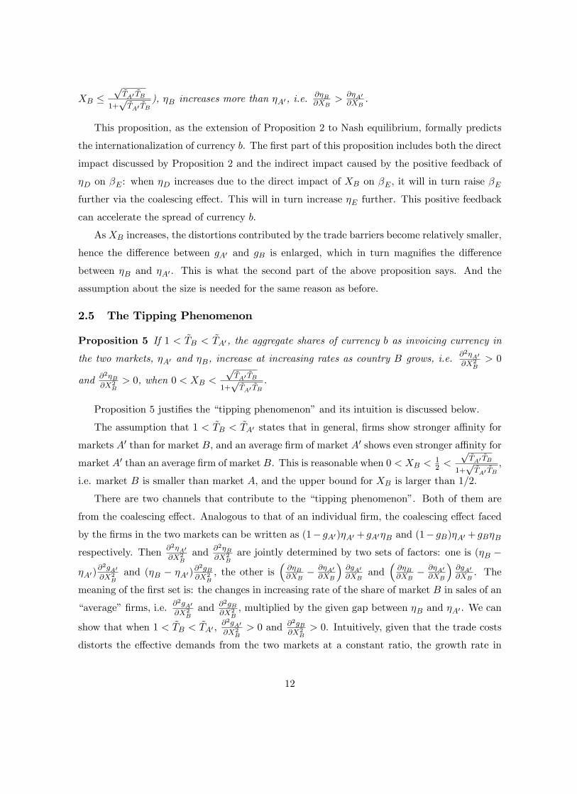
Figure 1 shows the relative importance of the two channels for �B (� = 5, = 0:76,

XB = 0:25 and Md = 0:3). The parameter combinations within the whole range in the graph

sustain the convexity. And the direct channel dominates when eTA0= eTB is below the blue line (asmaller gap between eTA0 and eTB) while the indirect channel dominates when eTA0= eTB is abovethat (a larger gap between eTA0 and eTB).

9 @�Bb@XB

� @�A0b@XB

/ 1[1�(gB�gA0 )]2

@(gB�gA0 )@XB

(Appendix 5.6) and (gB � gA0) is basically correlated with the gapbetween ~TA0 and ~TB in a positive way.

13

Figure 1 Relative importance of the two channels

Proposition 4 lays the foundation for the following prediction: when �tipping phenomenon�

holds, currencies of large countries would occupy disproportionately larger shares of aggregate

invoicing currency (see Figure 2). Consequently large countries gain excess advantages in the

international statuses of their currencies.

14

Figure 2 �Tipping phenomenon�

We next discuss the role of the trade cost eTA0 and eTB. They are essential to the convexityalthough they are not necessary for the internationalization itself. In other words, it a¤ects the

slope of the curve �D as a function of XB but does not a¤ect the positive sign of the slope.

The presence of trade costs satisfying eTA0 > eTB > 1 distorts the curve by compressing the

shares of the currency at aggregate level, with a larger degree when XB is smaller. In addi-

tion to trade costs in traditional sense, the rationale behind this assumption comes from the

network externality or economics of scale that favors the established international currencies.

Countries prefer to use whatever currency others use. Then once a currency becomes a vehicle,

the choice of vehicle is self-justifying. Using an analogy with language (Krugman 1984), what

makes English the world�s lingua franca is not its simplicity or internal beauty, but its wide

use. Once it is spoken among people whose native languages are not English, it is increasingly

so. Similarly, an exporter chooses a currency, in the belief that other exporters are also likely

to choose this one. Therefore, a list of advantages associated with this network externality,

such as lower transaction costs, fully convertibility, open �nancial asset transaction and easily

accessible �nancial services o¤ered, are all conducive to the well-grounded international curren-

cies. However, as one may already realize, to a new international currency, this type of network

externality is actually a counteracting force rather than a driving force. And this is hard to

15

avoid.10

This gives rise to the �tipping phenomenon�(orginally observed in o¢ cial reserve holdings):

�if one currency were to draw even and surpass another, the derivative of reserve currency use

with respect to its determining variables would be higher in that range than in the vicinity of

zero or in the range when the leading currency is unchallenged.� (Chinn and Frankel 2008).

By comparison, if without trade costs, the share of a currency in trade invoicing would simply

increase linearly with its home country�s size.

To look at a broader range of XB, we consider the following simple and symmetric case:

country A and country B are the only two big players in the world. When 0 < XB < 12 ,

1 < ~TB < ~TA0 , that is, �rms have more a¢ nity to market A0 in general; when XB = 12 ,~TB =

~TA0 = 1, �rms have the same a¢ nity to both markets and when 12 < XB < 1,

~TB < ~TA0 < 1,

�rms have more a¢ nity to market B. Then we can obtain the following corollary:

Corollary 1 When 0 < XB < 12 ,

@2�A0@X2

B> 0 and @2�B

@X2B> 0. When XB = 1

2 ,@2�A0@X2

B= @2�B

@X2B= 0.

When 12 < XB < 1,

@2�A0@X2

B< 0 and @2�B

@X2B< 0.

Interestingly, this corollary justi�es the curve in Krugman (1984) (it is replicated in Figure

3). There the x-axis is the actual use of the international currency (U.S. dollar in that case)

and the y-axis is the desire use of the currency. Therefore, the equilibrium point is the �xed

point, the intersection point between the curve and the 45 degree line. For comparison, the

curve indicated by Corollary 1 is depicted in Figure 4. Each point on this curve is already the

equilibrium point corresponding to the GDP share. Though slightly di¤erent in presentation,

the ideas are comparable. In that paper, the equilibrium that is attained among multiple

possible candidates is implicitly determined by fundamentals while we will show later that the

economic size of its home country is the most important fundamental, even the fatal one (think

that dollar was dethroned �nally despite the hysteresis). Krugman uses that graph to illustrate

the possible collapse of dollar. He shows that if the fundamental strength of the dollar keeps

deteriorating, the role of the dollar would �rst stand for a while, with gradual declining. But

once it falls beyond some critical level, the role of the dollar would drop dramatically to a

remarkably lower point and stay there even the fundamentals cease to weaken any further.

Figure 4 also sheds some light on the possible sharp decline. The slope in the middle range

10Matsuyama et al (1993) and Helene Rey (2001) discuss natural evolutions of international currencies frominternational trade.

16

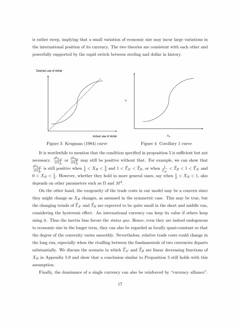
is rather steep, implying that a small variation of economic size may incur large variations in

the international position of its currency. The two theories are consistent with each other and

powerfully supported by the rapid switch between sterling and dollar in history.

Figure 3 Krugman (1984) curve Figure 4 Corollary 1 curve

It is worthwhile to mention that the condition speci�ed in proposition 5 is su¢ cient but not

necessary. @2�A0@X2

Bor @2�B

@X2Bmay still be positive without that. For example, we can show that

@2�A0@X2

Bis still positive when 1

2 < XB <23 and 1 <

~TA0 < ~TB, or when 1~TA0

< ~TB < 1 < ~TA0 and

0 < XB <12 . However, whether they hold in more general cases, say when

12 < XB < 1, also

depends on other parameters such as and Md.

On the other hand, the exogeneity of the trade costs in our model may be a concern since

they might change as XB changes, as assumed in the symmetric case. This may be true, but

the changing trends of eTA0 and eTB are expected to be quite small in the short and middle run,considering the hysteresis e¤ect. An international currency can keep its value if others keep

using it. Thus the inertia bias favors the status quo. Hence, even they are indeed endogenous

to economic size in the longer term, they can also be regarded as locally quasi-constant so that

the degree of the convexity varies smoothly. Nevertheless, relative trade costs could change in

the long run, especially when the rivalling between the fundamentals of two currencies departs

substantially. We discuss the scenario in which eTA0 and eTB are linear decreasing functions ofXB in Appendix 5.9 and show that a conclusion similar to Proposition 5 still holds with this

assumption.

Finally, the dominance of a single currency can also be reinforced by �currency alliance�.

17

There are two typical examples: one is follower countries which peg their currencies to the

currency of their leader country, such as Canadian dollar and Mexican peso to U.S. dollar; the

other one is monetary unions like the euro area. In such cases, the e¤ective size is actually the

combined economic size rather than the issuing country alone. Their combination would be

further augmented by the coalescing e¤ect, reducing the possible candidates for international

currencies to only a few ones and driving one or two eventually to dominate.11 This is consistent

with our common sense. With this logic, a common currency issued by a monetary union would

occupy a larger share of aggregate invoicing currency than the sum of the shares invoiced by

its member countries in the their own currencies.12 This explains the internationalization of

euro.

2.6 Hypotheses

According to the theoretical implications, we can test the following hypotheses:

Hypothesis 1: For a su¢ ciently large country, �rms in its small trade partner countries use

its currency as invoicing currency more than its big trade partner countries.

Hypothesis 2: As a country grows relative to the rest of the world, its currency is used more

as invoicing currency. Moreover, �rms in its small and close trading partners adjust their

invoicing currency more rapidly than those in its larger and less close trading partners.

Hypothesis 3: A currency is used as invoicing currency more in the issuing country than in

the trading partners. The currency is used more in countries that trade more with the isssuing

country than in countries that trade less with it. Moreover, the gap between the shares in the

close and distant trading partners increases as the size of the home country grows.

Hypothesis 4: There exists a �tipping phenomenon� in the global use of a currency for

invoicing purposes.

As mentioned in the introduction, �tipping phenomenon�could be observed not only over

a long time horizon for a given currency, but also across currencies at a given time. For

empirical tests, the observation along the time dimension for a given country imposes a higher

requirement on data quantity and quality, while the observation across countries at a given

time does not. So it is easier for us to test it in a �cross-sectional�way.

11 It could be another reason for �tipping phenomenon�. Although we do not explicitly explore this channel,we do consider it in our empirical work.12Bacchetta and van Wincoop (2005) has a similar conclusion for the invoicing currency of a monetary union,

but via a di¤erent channel.

18

3 The invoicing currencies in international trade

The empirical tests are conducted as follows: hypothesis 1 and 2 are tested with a data set

similar to the one built by Goldberg and Tille (2008) but extended to more countries and later

years. Hypothesis 3 and 4 are tested with another data set documenting multiple invoicing

currencies used in Thailand�s international trade. We �rst introduce the data sets, and then

show the econometric results of the tests in parts.

3.1 Data

The data in the �rst set is mainly from the reports �The international role of Euro�published

by European Central Bank, supplemented by reports from central banks of individual countries

(U.K., Australia and Thailand)13 and complied by us. They report the annual use of euro and

dollar as invoicing currencies at country level. There are totally thirty-�ve countries covered.

They are nine euro-area countries (Belgium, France, Germany, Greece, Italy, Luxembourg,

Netherlands, Portugal and Spain), thirteen European Union accession countries (Bulgaria,

Cyprus, Czech Republic, Denmark, Estonia, Hungary, Latvia, Lithuania, Poland, Romania,

U.K., Slovakia and Slovenia),14 three European Union candidate countries (Croatia, Former

Yugoslav Republic of Macedonia and Turkey), one other European country (Ukraine) and nine

countries outside Europe (Algeria, Australia, India, Indonesia, Pakistan, South Africa, Korea,

Thailand and Tunisia). We set the earliest observations in 1998, just one year before the euro

is introduced, and the latest observation is in 2010 (not balanced).15 As far as we know, this

is the most comprehensive data set on invoicing currencies across countries.

The data in the second set is from the central bank of Thailand. It includes all the invoicing

currencies they use (mainly U.S. dollar, euro, British pound sterling, Japanese yen, Thai baht,

and Deutsche mark) and their respective shares in trade between Thailand and �fteen Euro-

pean Union countries (Austria, Belgium, Denmark, Finland, France, Germany, Greece, Ireland,

Italy, Luxembourg, Netherlands, Portugal, Spain, Sweden and United Kingdom), three North

America countries (United States, Canada and Mexico) as well as Japan in 2001-2008 (bal-

anced). Obviously, a great virtue of this data set is that it provides the composition of multiple

invoicing currencies, which allows us to test �tipping phenomenon�. According to their inter-

13For details of this data set, please refer to the NBER working paper #11127 and Kamps (2006).14Slovenia, Cyprus and Slovakia join the euro during 2007-2009. We repeat our test by adjusting for this and

�nd the results almost unchanged.15The latest observation in Goldberg and Tille (2008) is roughly in 2003.

19

national positions, we focus on the four major international currencies � dollar, euro, sterling

and yen.

3.2 Comparison between currency invoicing in large countries and smallcountries

Hypothesis 1 and 2 are tested with the following general speci�cation:

�tcur;i = �0 + �1 thome;i + �2

thome;i

Y tiY thome

+ �3Heuroti + �4EU

+�5yeareuro + �6yeareuroY tiY thome

+ �ti

The dependent variable �tcur;i is the share of euro or dollar in export or import invoicing of

country i in year t. Hence we have four sets of regressions: euro�s share in exports, dollar�s share

in exports, euro�s share in imports and dollar�s share in imports. In general they corresponds to

the �E rather than the �E in our model because each country is supposed to be small and take

other countries�choice as given. Besides, the import invoicing currencies are also examined,

which seems strange with our model for export invoicing. However, we will explain along with

the results that the import invoicing can help us understand the theory from the perspective

of markets.

All the explanatory variables are chosen to correspond their dependent variables. Taking

the �rst dependent variable (euro�s share in exports) as example, thome;i is the share of euro

area in a country�s exports (here the home country of euro is euro area); Y tiY thome

is the size of the

exporting country relative to the euro area; EU is an indicator variable for EU membership.

Heuroet is the currency preference for cost hedging following Goldberg and Tille (2008). To

a speci�c country, it is 1 when euro is a preferred hedging currency on export transactions

(U.K. in our sample), 0 when euro and dollar are indi¤erent for hedging and -1 when dollar is

a preferred hedging currency (Estonia, Hungary and Thailand in our sample). yeareuro is the

number of years after the introduction of euro, taking 1998 as the base year.

The role of the �rst interaction term thome;iY ti

Y thomemay be more interesting than one might

think. According to our model, small countries are more willing to use the emerging interna-

tional currency because they are more reliant on trading with this emerging market. However,

this is already re�ected by the �rst term thome;i. The interaction term re�ects another reason

pointed by our assumption: large countries have a non-negligible mass of domestic sellers who

typically use their own currencies and their foreign currency followers (recall the equilibrium

20

condition for �B16). In this way, given the same reliance on trade with this particular coun-

try (the same thome;i), a large country uses its partner�s currency less in general. An typical

example is the U.K. Though both U.K. and its pound sterling have lost their preeminence for

long, sterling is still used with a notable degree for its domestic and neighborhood business.

By comparison, we could expect that for a small country, the weak in�uence of its own cur-

rency, home or abroad, would give the way to euro, even thought it has the same euro share

of export/import as U.K. By the way, the second interaction term yeareuroY ti

Y thomecontains the

both reasons for the contrast between large countries and small countries.

The role of the the time trend variable yeareuro also needs discussion. According to hypoth-

esis 2, the internationalization of a currency is promoted by the growth of its home country.

In euro�s case, it is captured by this time trend variable because the euro area�s GDP share

Xeuro, exploding immediately at the introduction of euro, is further enlarged gradually after-

wards, as more and more EU countries join the the euro (Slovenia from 2007, Cyprus and

Malta from 2008, and Slovakia from 2009, etc.). Besides, this time variable also contains the

inertia in adjustments by countries. The interaction term yeareuroY ti

Y thomecatches the di¤erence

in adjustment paces of small and large countries.

Table 1 presents the results from the speci�cation for the euro invoicing in exports. Ex-

planatory variables are introduced and accumulated one by one.17 As expected, the share of

euro area in country exports is strongly positive for the use of euro and contributes more than

60% to the explanatory power to account for the cross-country and intertemporal variation

of euro�s share in export invoicing. This corroborates the necessity to distinguish countries

according to their trade relationship with the home country.

The negative and signi�cant coe¢ cient estimates before the second explanatory variable

shows that euro is less used in exports by countries that are relatively large, with the share

of exports to euro area controlled. This result is quite similar to those of Goldberg and Tille

(2008), both in quality and quantity. The magnitude of this coe¢ cient drops nearly by half

when the second interaction term is introduced (last column) since these two terms are partially

correlated.

EU members use euro more widely, suggested by column (3). This is natural and also an

evidence for hypothesis 3. However, the hedging motive seems not important in our results.

16 In this sense, rather than �EB only, the dependent variables also include the component of �Eb.17To examine the vehicle roles of euro and dollar, we eliminate euro area countries for euro invoicing analyses

and include them for dollar invoicing analyses.

21

This validates our simpli�cation that cost hedging term is approximately zero in the model.

The time trend yeareuro enters with signi�cant and positive coe¢ cient, supporting hypoth-

esis 2. In general, the use of euro increases over time. What is more, the increase is contributed

by smaller countries with a relatively larger degree, signi�ed by strongly negative coe¢ cient

for the interaction term yeareuroY ti

Y thome. If one takes a further inspection into the data, she will

�nd that relatively large countries, such as U.K., Australia and Denmark, are indeed slower

adjustors.

The last column incorporates transaction cost into the regression. The transaction cost is

calculated in a way that is standard in literature18 � the median di¤erence in pips on using

euros versus pips on using dollars for each year. Consistent with Goldberg and Tille (2008), it

is insigni�cant to explain invoicing currency choice.19

Table 2 presents the results for dollar invoicing in exports. The features showed by the �rst

two coe¢ cients are similar to euro. But the magnitude of the coe¢ cients before the second

term are much larger. This is because we use the GDP of each member country in EU rather

than the GDP of the whole EU. If we replace it with the GDP of the whole EU, the coe¢ cient

will fall to roughly �2:5 but still show signi�cance at 1% level (not reported). The features

showed by the last four coe¢ cients are almost opposite to the euro case, which are reasonable

as euro and dollar are competitors, at least in Europe. The negative coe¢ cient before the

time trend supports what we predict for monetary union in section 2: even though euro gains

popularity mainly at the expense of the original currencies of its member countries, it crowds

out the dollar in Europe a little bit. And the last term shows that larger countries are obviously

slow responders to this change.

Table 3 and 4 report the results from euro and dollar invoicing in imports. We can interpret

the results from the perspective of markets. Intuitively, suppose we decompose �A0 into �A and

�C , we could expect that in equilibrium �A < �C < �B. The logic is similar to the interpretation

for the interaction term thome;iY ti

Y thome: small countries have fewer currency followers home or

abroad. And with less mass as ballasts, import invoicing currency of small countries will also be

a¤ected more easily. Thus we expect the import invoicing currencies to share similar patterns

with those of export invoicing currencies.

18Goldberg and Tille (2008) and Chen Hongyi et al (2009)19Since some missing observations in data for transaction costs limit the total observations we can use, we

report the results without it from now on. However, when we repeat our analysis with it, the results are almostunaltered, as in column (7).

22

Generally speaking, they indeed do. Nonetheless, the time trend term yeareuro is not

signi�cant in the case of dollar in import invoicing. This implies that a world-wide �average�

exporter does not lessen the use of dollar as invoicing currency. In other words, euro is more

a regionally international currency than a globally internationally currency. But the pace

di¤erence still stands for both euro and dollar. Further, if we restrict our sample to EU

member countries in the last case, the desired patterns are much stronger (column 7 in Table

4). This, again, reminds us that the variations of trade relationship or di¤erent extents of

economic integration among countries should not be ignored to understand the breadth and

depth of internationalization of a currency.

3.3 Comparison across invoicing currencies

For comparison across multiple invoicing currencies, the second data set has an obvious limi-

tation � its narrow coverage (only Thailand�s trade). But we can turn this disadvantage to

an advantage when testing hypothesis 3. With one partner of the trade being controlled, we

obtain a check on the di¤erent in�uences of an international currency in di¤erent geographic

areas, and verify hypothesis 3 straightforwardly. The data reports the aggregate compositions

of invoicing currencies between Thailand and three trade unions: EU 15, NAFTA, and ASEAN.

The shares of U.S. dollar, euro, British pound sterling and Japanese yen in Thailand�s export

invoicing to these three unions and their home countries�global GDP shares are scattered in

Figure 5.

23

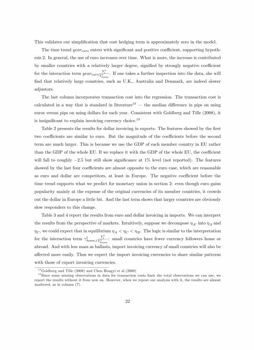
Figure 5 Four international currencies: export invoicing share to ASEAN/EU/NAFTA

versus its home country�s GDP share

It is clear that regardless of the destination, dollar is the absolute number one invoicing

currency, while euro is the number two, ahead of yen and pound sterling. Beyond that, two

patterns are noteworthy: �rst, an international currency gains more acceptance in their home

and neighborhood markets, namely, U.S. dollar to NAFTA, euro and sterling to EU, and

Japanese yen to ASEAN, respectively. Second, the larger is the home country, the larger is the

gap. The four sub�gures are ranked at a descending order of its home country�s size. Obviously,

the gap associated with dollar is the largest, followed by that associated with euro, and the gaps

corresponding to yen and sterling are much smaller.20 These characteristics are also signi�cant

in Thailand�s import invoicing (see Figure 7 in Appendix ).

20 If one regress the invoicing shares of each currency on the dummy of its home, the rank of the coe¢ cientestimates (all positive) is also consistent with the rank of GDP share except for Japanese yen. This is probablybecause Japan adopts a pricing-to-market policy which encourages exporters to invoice in local currency offoreign markets (Takatoshi et al 2010). From another perspective, this policy a¢ rms the mechanism of thecoalescing e¤ect.

24

3.4 �Tipping phenomenon�

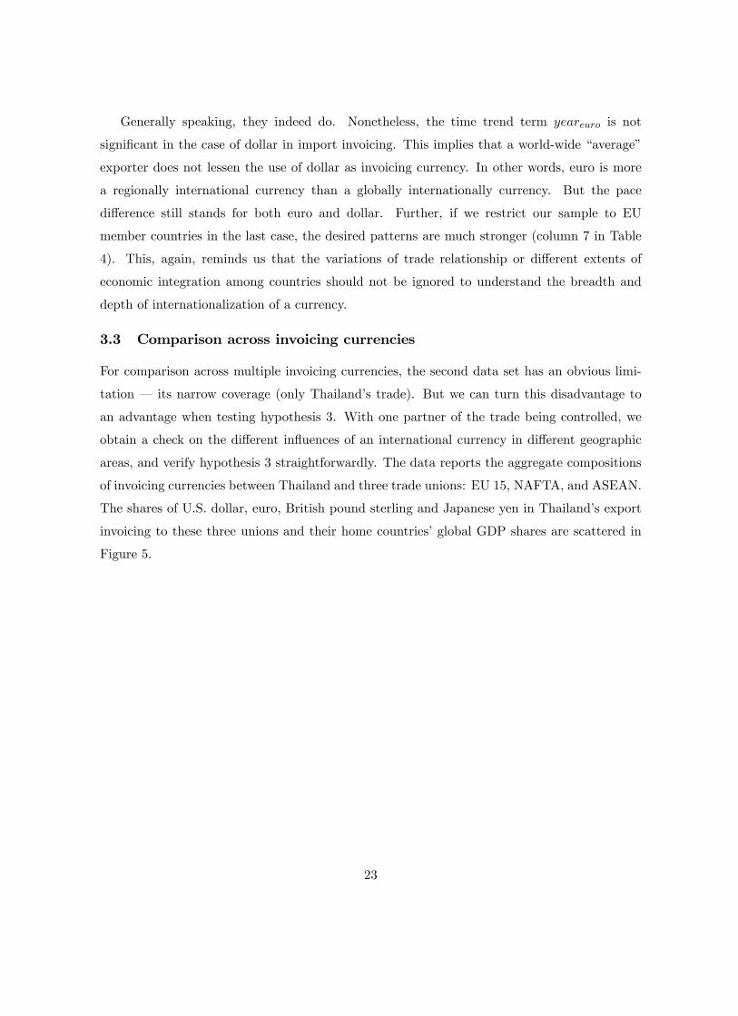
Chinn and Frankel (2007) document a strong non-linear relationship between currency shares

in o¢ cial reserves and GDP shares. A similar �tipping phenomenon�is expected to be observed

in invoicing currencies. However, there is rarely any econometric study on this, since the data

on trade invoicing-currency is much less comprehensively quanti�able than that on reserve

currency holdings.

Figure 6 displays the shares of the four currencies in trade invoicing to EU 15 countries in

2001-2008. The existence of �tipping phenomenon�is apparent from inspection of the diagram.

Figure 6 Invoicing currency share versus GDP share (left: export; right: import)

To examine the �tipping phenomenon�, we compare the �tness between the following two

speci�cations:

�tcur = �1xtissuer + �2

tpartner;issuer + �3

tThailand;issuer + �4(bid� ask)tcur;baht

+�5regime+ "tcur

log �tcur1��tcur

= �1xtissuer + �2

tpartner;issuer + �3

tThailand;issuer + �4(bid� ask)tcur;baht

+�5regime+ �tcur

The two speci�cations only di¤er in the form of the dependent variable. The one in the second

is the logit transformation of the one is the �rst. The logit function f(x) = log x1�x is concave

when 0 < x < 12 and convex when

12 < x < 1. Therefore the non-linearity embedded in the

�tipping phenomenon�as well as the Krugman (1984) curve can be o¤set by this transformation,

leading to better linear �tness. So the improvement in the linear �tness when moving from the

�rst speci�cation to the second is an indicator for the strength of the non-linearity.

25

Among the independent variables, xtissuer is the GDP share of the issuing country of one

particular international currency in year t. The variables tpartner;issuer and tThailand;issuer

are the shares of exports (imports) to the issuing country in the total exports (imports) of

that partner country and Thailand, respectively. If the partner country happens to be the

issuing country, we set tpartner;issuer = 1. The variable pip(cur� baht)t is the transaction costsbetween Thai Baht and the currency in question. The variable regime is the extent to which

the exchange rate of the currency of the partner country �uctuates with the exchange rate of

that international currency, with respect to the same base currency.

As mentioned in the section 2, the exchange rate regime could be another determinant for

invoicing currency decision, so we include it into our regression. The more an international

currency weighs in a country�s currency basket, the more preferable it is to the exporters from

this country. To measure the relative weight of major international currencies in one country�s

currency basket, we adopt the method introduced by Frankel and Wei (1994) and applied by

other studies.21 More speci�cally, we use the daily exchange rate data from Bloomberg (last

price)22 and run the following regression

� log(Spartnercurrency=SwissFranc) = �1� log(SUSD=SwissFranc) + �2� log(SEUR=SwissFranc)

+�3� log(SGBP=SwissFranc) + �4� log(SJPY=SwissFranc)

+�0 + �tpartnercurrency

The �uctuations of exchange rates of four major international currencies are utilized to

explore the �uctuations of the exchange rate of a national currency, by taking Swiss Franc as

the base currency. The coe¢ cients suggest the weight of one international currency in this

country�s currency basket.23 Our estimates show that in North America, Canadian dollar

partially comove with U.S. dollar while Mexican peso is almost completely pegged to U.S.

dollar. U.K., Denmark and Sweden are the non-euro countries among the �fteen EU countries.

Danish krona is closely pegged to euro while Swedish krona comove with euro with a very low

degree.

Unlike studies that attempt to ascertain the determinants of the international role of a

currency, we do not include a lagged variable such as �t�1cur , because this variable is highly

21e.g. Eichengreen (2006) and Frankel (2007)22The period is Jan.1st 2001 to Dec. 31st 2008. We estimate the coe¢ cients on a year basis.23but not equal to that weight exactly. See Frankel and Wei (1994).

26

correlated with the xthome, as one can expect. What we want to capture is a long run trend of

the relationship between the vehicle currency role and its home country�s economic size.

Table 5 and 6 present the comparisons before and after logit transformation in pairs. Quite

clearly, for each pair with exactly the same sample, judged by the adjusted R2, the speci-

�cations after logit transformation are systematically more successful to explain the shares

of international currencies in invoicing. In fact, considering the automatic elimination of the

observations of zero values by the transformation, our estimations about the �tipping phenom-

enon�are actually downward biased since these observations can sharpen the contrast across

currencies.

The economic size measured by GDP share accounts for more than 50% of di¤erences in

the invoicing currency shares, showed by column (1) and (2). This establishes the absolute

dominance of economic size among a number of economic fundamentals (current account sta-

tus, in�ation rate as well as appreciation/depreciation and so forth). Besides, the additional

explanatory power with logit transformation is mainly contributed by an obvious rise in the

signi�cance of this term, which precisely indicates the non-linearity. This echoes a similar �nd-

ing in Chen Hongyi et al (2009). They demonstrate that the global GDP share is remarkably

more important than other fundamental variables to account for the currency shares of reserve

holdings.

As expected, the share of the international-currency-issuing country in total export/import

of one country tpartner;home enters with positive signs. However, it may be puzzling that the

share of the issuing country in total import of Thailand tThailand;home enters with negative

signs. This is because the descending order of trade closeness of Thailand�s importing partners

is Japan, EU 15, U.S. and U.K. which happens to be negatively correlated with their economic

sizes. On the other hand, we can interpret the strength and the robustness of the role of

economic sizes from this result, as the country-speci�c trade relationships are not able to

distort the positions of international currencies, even locally.

Another two interesting points are with respect to the e¤ects of transaction costs and

exchange rate regime. Unlike the previous tests, the transaction cost is signi�cant in this test.

Trade partner involved here do concern about the transaction costs. A possible reason for that

is it could be easier and less expensive for exporters from European countries (the majority

in the �rst sample) to switch between euro and dollar than for Thai �rms to convert baht to

dollar, euro, sterling or yen.

27

The negative signs of the coe¢ cients before the exchange regime term also seem unexpected.

This is because the majority of the sampled countries are European countries which do not peg

to U.S. dollar but to euro. This, just as the export/import share discussed above, indirectly

corroborates the notable dominance of economic size in determining the international status

of a currency. If we control for the currency type, this coe¢ cient will become positive (not

reported).

Finally, the �tipping phenomenon�can also be tested in speci�cation with quadratic form or

cubic form (see Table 7). With the quadratic form, the second order term is strongly positive,

supporting the non-linearity. With the cubic form, the third order term is also signi�cant, with

a negative sign. This implies that when GDP share is relative smaller (smaller than 0.20 in this

case), the non-linearity is convexity while when the GDP share is relative larger (larger than

0.20), the non-linearity turns to concavity. In terms of the number of statistically signi�cant

coe¢ cients, the cubic form �ts better. Thus it indicates a possibility that although the economic

power of U.S. does not completely dominate (its global GDP share is about 20%-30%), dollar

is already positioned on the second half of the Krugman curve.

4 Conclusion

We develop a theory to explain the emergence of a currency as a vehicle currency for trade

settlement as the issuing country�s economic size grows relative to the rest of the world. The

fundamental mechanism for the dynamics of the emergence of the currency is the coalescing

e¤ect: exporters have strong incentive to use the currency mix that their competitors use to

invoice their exports. When a country�s market expands, exporters to that market tend to use

a larger share of the local currency to invoice its exports. Since exporters would require the

price levels across markets to be not so di¤erent as to allow goods-arbitrage to occur, the use

of the currency in its home and nearby markets would spread to other markets. The positive

feedback between the use of a currency as a vehicle currency by an individual �rm and that by

its competitors helps to accelerate the use of that currency for trade settlement.

Furthermore, the propagation would start from its smaller and closer trading partners to

larger and less close trading partners. This is because the smaller and closer partners often have

higher trade/GDP ratio with this rapidly growing country and the smaller countries�currencies

are less likely to be used by domestic and foreign �rms as invoicing currencies. On the contrary,

the larger and less close partners have lower trade/GDP ratios with the growing country, and

28

the larger countries� currencies are more likely to be used by domestic and foreign �rms as

vehicle currencies. Consequently, the emerging currency would gain acceptance from countries

that rely more on trade with the emerging country before the acceptance is spread to countries

that rely less on trade with the emerging country.

More importantly, we derive a non-linear but positive relationship between the share of

global use of a currency as an invoicing currency and the economic size of the issuing country.

We show that the relationship is convex when the economic size of the issuing country is

small relative to the rest of the world and concave when it is relatively large. This con�rms

Krugman�s (1984) curve. The convex part corresponds to the tipping phenomenon in the

sense that currencies of larger countries have disproportionately higher share of global use as

vehicle currency. This non-linearity is generated by the smaller transaction cost associated

with the established international currency compared with that associated with the currency

of the emerging economy. With these frictions favoring the established international currency,

the global use of the currency of an emerging country increases very slowly in the beginning,

even as the country grows very fast. However, this rate of increase accelerates as the country�s

relative size continues to grow. When the economic size of the country reaches a certain tipping

point, the global use of its currency can abruptly increase, and it becomes a widely used vehicle

currency in a relatively short period of time. When the currency gains su¢ cient dominance as

a vehicle currency, the rate of increase of its global use decelerates even as the relative economic

size of the issuing country continues to grow. This corresponds to the concave part of the curve.

Although our model makes use of many simplifying assumptions, it is su¢ cient to capture

the basic insights and intuition behind the mechanism at work. Moreover, the hypotheses

generated by the theory are testable, and tested, using the scarce and scattered data on invoicing

currencies in a number of countries. The empirical results are consistent with the implications

of the model. The results also strongly indicate the signi�cance of (i) the share of global trade

of the issuing country as well as (ii) its relative economic size, in determining the share of

global use of the currency for trade settlement. These channels are also predicted to be of great

signi�cance by our theory.

Our theory and the empirical evidence show that one should expect the pace of increase in

the global use of the Chinese RMB for trade settlement to be slow in the near future, even as

China grows fast relative to the rest of the world. This is so especially because China�s �nancial

system is quite immature and underdeveloped, and the RMB is not fully convertible. Besides

29

tackling these shortcomings of its �nancial system, China can speed up internationalization

of the RMB by facilitating the coalescing e¤ect to take place, as well as facilitating its major

trading partners (i.e. the smaller or closer countries) to use RMB for trade settlement by

making it less costly for these foreign �rms to buy and sell RMB. Some of these measures have

already been undertaken in recent years.24

24For instance, the central bank of China has signed currency swap contracts with central banks of twentycountries. The countries are mainly in Asia, including South Korea and Japan.

30

References

[1] Bacchetta Philippe and Eric van Wincoop, 2005, �A theory of the currency denomination

of international trade�, Journal of International Economics, 67, 295-319

[2] Chen, Hongyi; Wensheng Peng; Chang Shu. 2009. �The Potential of the Renminbi as

an International Currency,� manuscript, Hong Kong Institute for Monetary Research,

February 2009.

[3] Chinn Menzie and Frankel Je¤ery, 2007, �Will the Euro Eventually Surpass the Dollar

as Leading International Reserve Currency?�in G7 Current Account Imbalances: Substan-

tiality and Adjustment, Richard H. Clarida (ed.), University of Chicago Press, 285-322

[4] Chinn Menzie and Frankel Je¤ery, 2008, �Why the Euro Will Rival the Dollar?�, Interna-

tional Finance, 11:1, 49-73

[5] Engel, Charles, 2006. Equivalence results for optimal pass-through, optimal indexing to

exchange rates, and optimal choice of currency for export pricing. Journal of the European

Economic Association 4 (6), 1249-1260

[6] Eichengreen, Barry, 2006, �China�s Exchange Rate Regime: The Long and Short of It.�

mimeo, University of California Berkeley

[7] Eichengreen, Barry, 2011, �The renminbi as an international currency,�Journal of Policy

Modeling, 33, 723-730

[8] European Central Bank, 2011, Review of the International Role of the Euro

[9] Frankel, Je¤rey, A. and Shang-jin Wei, 1994, �Yen Block or Dollar Bloc? Exchange Rate

Policies of the East Asian Economies,� in Macroeconomic Linkage: Savings, Exchange

Rates, and Capital Flows, edited by Ito, Takatoshi and Anne O. Krueger, Chicago: Uni-

versity of Chicago Press, 295-333.

[10] Fisher, Eric, 1989, �A model of exchange rate pass-through,� Journal of International

Economics 26, 119-138

[11] Friberg, Richard, 1998, �In which currency should exporters set their prices?�Journal of

International Economics, 45, 59-76

31

[12] Gita Gopinath, Oleg Itskhoki, and Roberto Rigobon, 2010, �Currency Choice and Ex-

change Rate Pass-Through�, American Economic Review, 100:1, 304-336

[13] Goldberg Linda, Tille Cedric, 2008, �Vehicle Currency Use in International Trade�, Jour-

nal of International Economics, 76, 177-192

[14] Hans Genberg, 2009. �Currency Internationalization: Analytical and Policy Issues�. Hong

Kong Institute for Monetary Research Working Paper No. 31/2009

[15] Helene Rey, 2001, �International Trade and Currency Exchange�Review of Economic Stud-

ies, 68, 443-464

[16] Kamps, Annette. 2006. �The euro as invoicing currency in international trade,�European

Central Bank working paper No.665 (August)

[17] Krugman, Paul R. 1980. �Vehicle currencies and the structure of international exchange.�

Journal of Money, Credit and Banking 12: 513-526.

[18] Krugman, Paul R. 1984. �The International Role of the Dollar: Theory and Prospect.�in

Exchange Rate Theory and Practice, John F.O. Bilson and Richard C. Marston (eds.),

University of Chicago Press, 261-278

[19] Oi, Hiroyuki, Akira Otani, and Toyoichiro Shirotam, 2004,�The Choice of Invoice Currency

in International Trade: Implications for the Internationalization of the Yen,�Monetary and

Economic Studies, 27-63

[20] Randall Wright and Alberto Trejos, 2001, �International Currency�, Advances in Macro-

economics, vol 1, iss 1, 1-14

[21] Rauch, James. 1999. �Networks versus Markets in International Trade,�Journal of Inter-

national Economics, 48, 7-35

[22] Swoboda, Alexander, 1969. �Vehicle currencies and the foreign exchange market: the case

of the dollar,�in The International Market for Foreign Exchange, Praeger Special Studies

in International Economics and Development, edited by Aliber, Robert Z. (ed.), Frederick

A. Praeger Publishers, New York.

[23] Kiyotaki, N. and Wright, R., 1989, �On Money as a Medium of Exchange,� Journal of

Political Economy, 97, 927-954

32

[24] Kiminori Matsuyama, Nobuhiro Kiyotaki and Akihiko Matsui, 1993, �Toward a Theory

of International Currency,�Review of Economic Studies, 60, 283-307

[25] McKinnon, Ronald, 1979, Money in International Exchange. New York: Oxford University

Press.

[26] Viaene, Jean-Marie, de Vries, Casper G., 1992, �On the Design of Invoicing Practices in

International Trade,�Open Economies Review, 3: 133-142

[27] Wilander, Fredrik, 2006, �An Empirical Analysis of the Currency Denomination in Inter-

national Trade,�manuscript, Stockholm School of Economics.

33

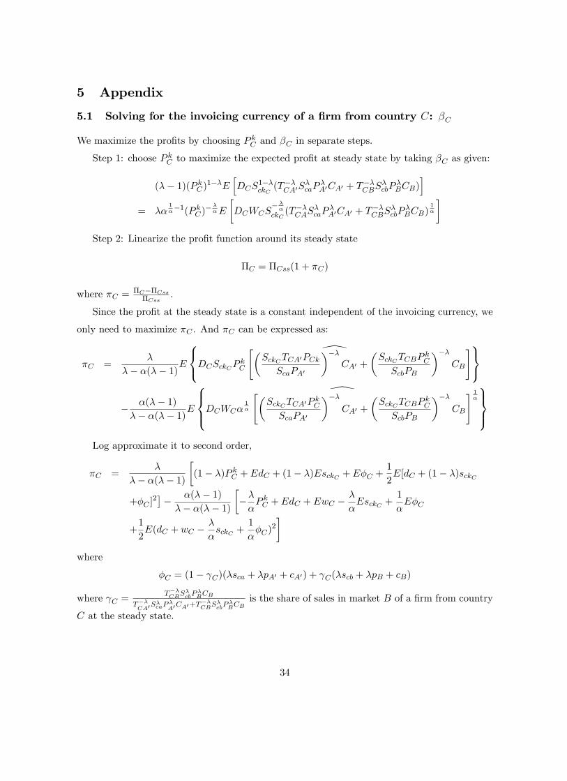
5 Appendix

5.1 Solving for the invoicing currency of a �rm from country C: �C

We maximize the pro�ts by choosing P kC and �C in separate steps.

Step 1: choose P kC to maximize the expected pro�t at steady state by taking �C as given:

(�� 1)(P kC)1��EhDCS

1��ckC

(T��CA0S�caP

�A0CA0 + T

��CBS

�cbP

�BCB)

i= ��

1��1(P kC)

� ��E

�DCWCS

� ��

ckC(T��CAS

�caP

�A0CA0 + T

��CBS

�cbP

�BCB)

1�

�Step 2: Linearize the pro�t function around its steady state

�C = �Css(1 + �C)

where �C =�C��Css�Css

.

Since the pro�t at the steady state is a constant independent of the invoicing currency, we

only need to maximize �C . And �C can be expressed as:

�C =�

�� �(�� 1)E

8<:\

DCSckCPkC

"�SckCTCA0PCkScaPA0

���CA0 +

�SckCTCBP

kC

ScbPB

���CB

#9=;� �(�� 1)�� �(�� 1)E

8><>:\

DCWC�1�

"�SckCTCA0P

kC

ScaPA0

���CA0 +

�SckCTCBP

kC

ScbPB

���CB

# 1�

9>=>;Log approximate it to second order,

�C =�

�� �(�� 1)

�(1� �)P kC + EdC + (1� �)EsckC + E�C +

1

2E[dC + (1� �)sckC

+�C ]2�� �(�� 1)�� �(�� 1)

����P kC + EdC + EwC �

�

�EsckC +

1

�E�C

+1

2E(dC + wC �

�

�sckC +

1

��C)

2

�where

�C = (1� C)(�sca + �pA0 + cA0) + C(�scb + �pB + cB)

where C =T��CBS

�cbP

�BCB

T��CA0S

�caP

�A0CA0+T

��CBS

�cbP

�BCB

is the share of sales in market B of a �rm from country

C at the steady state.

34

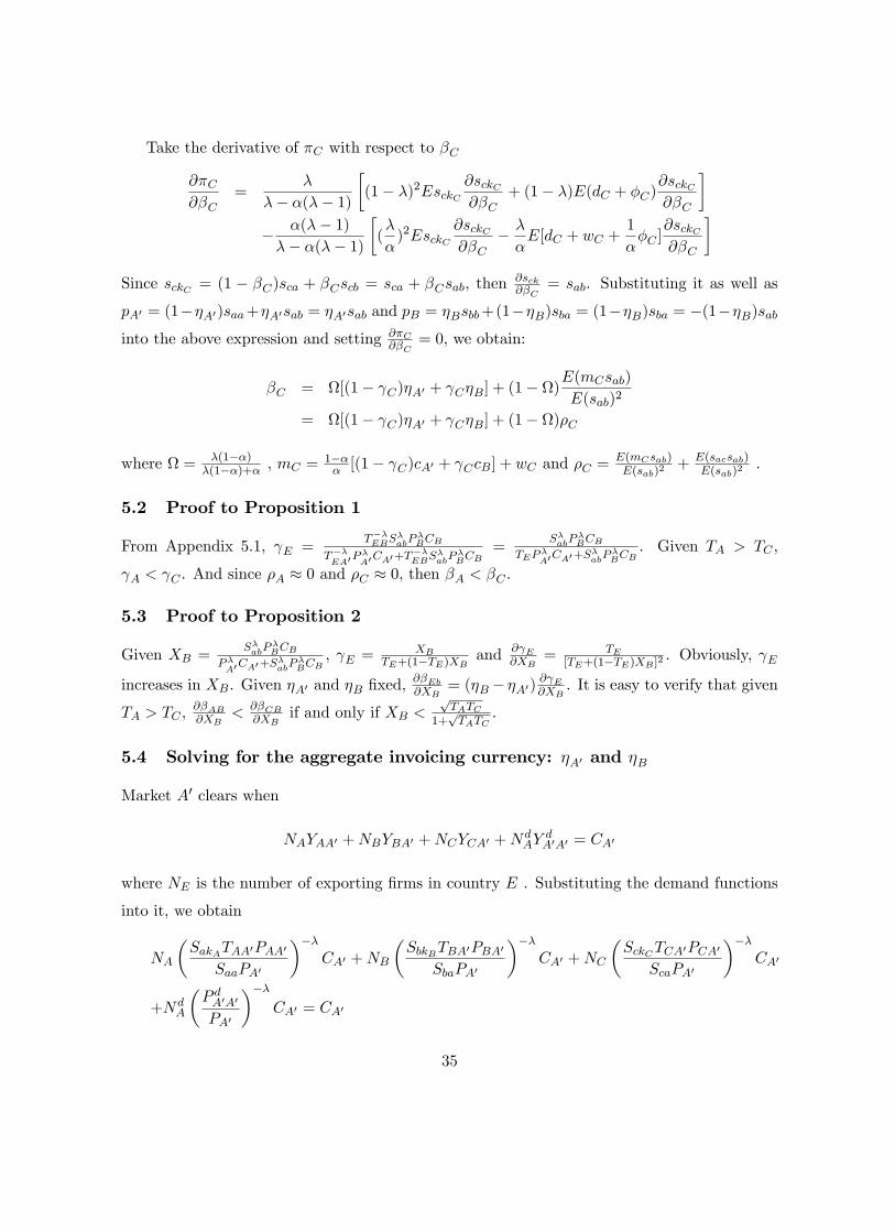
Take the derivative of �C with respect to �C

@�C@�C

=�

�� �(�� 1)

�(1� �)2EsckC

@sckC@�C

+ (1� �)E(dC + �C)@sckC@�C

�� �(�� 1)�� �(�� 1)

�(�

�)2EsckC

@sckC@�C

� �

�E[dC + wC +

1

��C ]

@sckC@�C

�Since sckC = (1 � �C)sca + �Cscb = sca + �Csab, then

@sck@�C

= sab. Substituting it as well as

pA0 = (1��A0)saa+�A0sab = �A0sab and pB = �Bsbb+(1��B)sba = (1��B)sba = �(1��B)sabinto the above expression and setting @�C

@�C= 0, we obtain:

�C = [(1� C)�A0 + C�B] + (1� )E(mCsab)

E(sab)2

= [(1� C)�A0 + C�B] + (1� )�C

where = �(1��)�(1��)+� , mC =

1��� [(1� C)cA0 + CcB] + wC and �C =

E(mCsab)E(sab)2

+ E(sacsab)E(sab)2

.

5.2 Proof to Proposition 1

From Appendix 5.1, E =T��EBS

�abP

�BCB

T��EA0P

�A0CA0+T

��EBS

�abP

�BCB

=S�abP

�BCB

TEP�A0CA0+S

�abP

�BCB

. Given TA > TC ,

A < C . And since �A � 0 and �C � 0, then �A < �C .

5.3 Proof to Proposition 2

Given XB =S�abP

�BCB

P�A0CA0+S

�abP

�BCB

, E =XB

TE+(1�TE)XB and @ E@XB

= TE[TE+(1�TE)XB ]2 . Obviously, E

increases in XB. Given �A0 and �B �xed,@�Eb@XB

= (�B � �A0)@ E@XB

. It is easy to verify that given

TA > TC ,@�AB@XB

< @�CB@XB

if and only if XB <pTATC

1+pTATC

.

5.4 Solving for the aggregate invoicing currency: �A0 and �B

Market A0 clears when

NAYAA0 +NBYBA0 +NCYCA0 +NdAY

dA0A0 = CA0

where NE is the number of exporting �rms in country E . Substituting the demand functions

into it, we obtain

NA

�SakATAA0PAA0

SaaPA0

���CA0 +NB

�SbkBTBA0PBA0

SbaPA0

���CA0 +NC

�SckCTCA0PCA0

ScaPA0

���CA0

+NdA

�P dA0A0

PA0

���CA0 = CA0

35

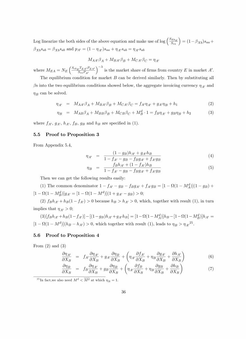
Log linearize the both sides of the above equation and make use of log�SEkESea

�= (1��Xb)saa+

�Xbsab = �Xbsab and pA0 = (1� �A0)saa + �A0sab = �A0sab

MAA0�A +MBA0�B +MCA0�C = �A0

where MEA = NE

�SekETEA0PEA0

SeaPA0

���is the market share of �rms from country E in market A0.

The equilibrium condition for market B can be derived similarly. Then by substituting all

�s into the two equilibrium conditions showed below, the aggregate invoicing currency �A0 and

�B can be solved.

�A0 = MAA0�A +MBA0�B +MCA0�C = fA0�A0 + gA0�B + h1 (2)

�B = MAB�A +MBB�B +MCB�C +MdB � 1 = fB�A0 + gB�B + h2 (3)

where fA0 , gA0 , hA0 ; fB, gB and hB are speci�ed in (1).

5.5 Proof to Proposition 3

From Appendix 5.4,

�A0 =(1� gB)hA0 + gA0hB

1� fA0 � gB � fBgA0 + fA0gB(4)

�B =fBhA0 + (1� fA0)hB

1� fA0 � gB � fBgA0 + fA0gB(5)

Then we can get the following results easily:

(1) The common denominator 1� fA0 � gB � fBgA0 + fA0gB = [1� (1�MdA)](1� gB) +

[1� (1�MdB)]gA0 = [1� (1�Md)](1 + gA0 � gB) > 0;

(2) fBhA0 + hB(1� fA0) > 0 because hB > hA0 > 0, which, together with result (1), in turnimplies that �A0 > 0;

(3)[fBhA0+hB(1�fA0)]� [(1�gB)hA0+gA0hB] = [1�(1�MdA)]hB� [1�(1�Md

B)]hA0 =

[1� (1�Md)](hB � hA0) > 0, which together with result (1), leads to �B > �A025.

5.6 Proof to Proposition 4

From (2) and (3)

@�A0

@XB= fA0

@�A0

@XB+ gA0

@�B@XB

+

��A0

@fA0

@XB+ �B

@gA0

@XB+@hA0

@XB

�(6)

@�B@XB

= fB@�A0

@XB+ gB

@�B@XB

+

��A0

@fB@XB

+ �B@gB@XB

+@hB@XB

�(7)

25 In fact,we also need Md < Md at which �B = 1.

36

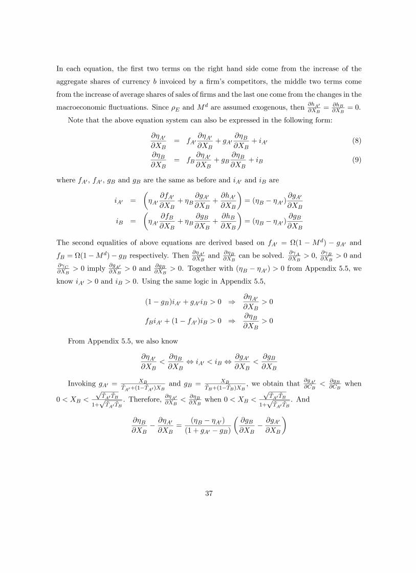
In each equation, the �rst two terms on the right hand side come from the increase of the

aggregate shares of currency b invoiced by a �rm�s competitors, the middle two terms come

from the increase of average shares of sales of �rms and the last one come from the changes in the

macroeconomic �uctuations. Since �E and Md are assumed exogenous, then @hA0

@XB= @hB

@XB= 0.

Note that the above equation system can also be expressed in the following form:

@�A0

@XB= fA0

@�A0

@XB+ gA0

@�B@XB

+ iA0 (8)

@�B@XB

= fB@�A0

@XB+ gB

@�B@XB

+ iB (9)

where fA0 , fA0 , gB and gB are the same as before and iA0 and iB are

iA0 =

��A0

@fA0

@XB+ �B

@gA0

@XB+@hA0

@XB

�= (�B � �A0)

@gA0

@XB

iB =

��A0

@fB@XB

+ �B@gB@XB

+@hB@XB

�= (�B � �A0)

@gB@XB

The second equalities of above equations are derived based on fA0 = (1 �Md) � gA0 andfB = (1�Md)� gB respectively. Then @�A0

@XBand @�B

@XBcan be solved. @ A

@XB> 0, @ B@XB

> 0 and@ C@XB

> 0 imply @gA0@XB

> 0 and @gB@XB

> 0. Together with (�B � �A0) > 0 from Appendix 5.5, we

know iA0 > 0 and iB > 0. Using the same logic in Appendix 5.5,

(1� gB)iA0 + gA0iB > 0 ) @�A0

@XB> 0

fBiA0 + (1� fA0)iB > 0 ) @�B@XB

> 0

From Appendix 5.5, we also know

@�A0

@XB<@�B@XB

, iA0 < iB ,@gA0

@XB<@gB@XB

Invoking gA0 =XB

~TA0+(1� ~TA0 )XBand gB =

XB~TB+(1� ~TB)XB

, we obtain that @gA0@CB

< @gB@CB

when

0 < XB <

p~TA0

~TB

1+p~TA0

~TB. Therefore, @�A0@XB

< @�B@XB

when 0 < XB <p~TA0

~TB

1+p~TA0

~TB. And

@�B@XB

� @�A0

@XB=

(�B � �A0)(1 + gA0 � gB)

�@gB@XB

� @gA0

@XB

�

37

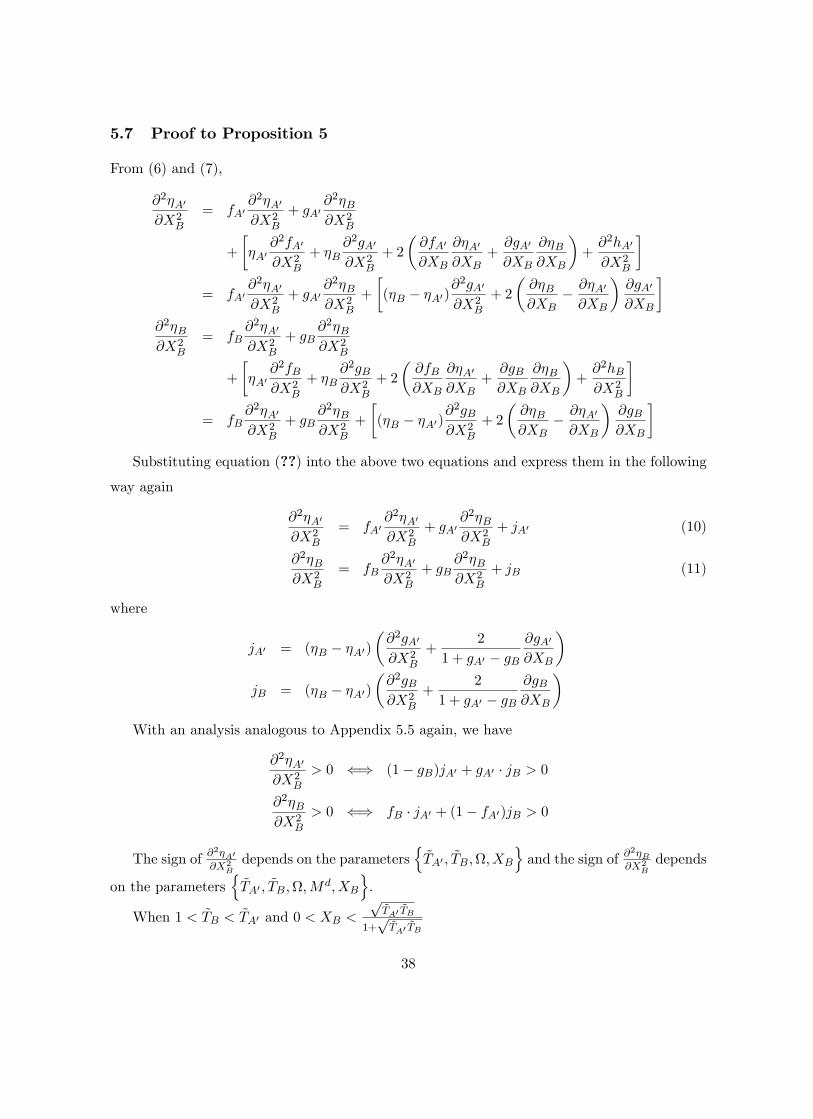
5.7 Proof to Proposition 5

From (6) and (7),

@2�A0

@X2B

= fA0@2�A0

@X2B

+ gA0@2�B@X2

B

+

��A0

@2fA0

@X2B

+ �B@2gA0

@X2B

+ 2

�@fA0

@XB

@�A0

@XB+@gA0

@XB

@�B@XB

�+@2hA0

@X2B

�= fA0

@2�A0

@X2B

+ gA0@2�B@X2

B

+

�(�B � �A0)

@2gA0

@X2B

+ 2

�@�B@XB

� @�A0

@XB

�@gA0

@XB

�@2�B@X2

B

= fB@2�A0

@X2B

+ gB@2�B@X2

B

+

��A0

@2fB@X2

B

+ �B@2gB@X2

B

+ 2

�@fB@XB

@�A0

@XB+@gB@XB

@�B@XB

�+@2hB@X2

B

�= fB

@2�A0

@X2B

+ gB@2�B@X2

B

+

�(�B � �A0)

@2gB@X2

B

+ 2

�@�B@XB

� @�A0

@XB

�@gB@XB

�Substituting equation (??) into the above two equations and express them in the following

way again

@2�A0

@X2B

= fA0@2�A0

@X2B

+ gA0@2�B@X2

B

+ jA0 (10)

@2�B@X2

B

= fB@2�A0

@X2B

+ gB@2�B@X2

B

+ jB (11)

where

jA0 = (�B � �A0)�@2gA0

@X2B

+2

1 + gA0 � gB@gA0

@XB

�jB = (�B � �A0)

�@2gB@X2

B

+2

1 + gA0 � gB@gB@XB

�With an analysis analogous to Appendix 5.5 again, we have

@2�A0

@X2B

> 0 () (1� gB)jA0 + gA0 � jB > 0

@2�B@X2

B

> 0 () fB � jA0 + (1� fA0)jB > 0

The sign of @2�A0@X2

Bdepends on the parameters

n~TA0 ; ~TB;; XB

oand the sign of @

2�B@X2

Bdepends

on the parametersn~TA0 ; ~TB;;M

d; XB

o.

When 1 < ~TB < ~TA0 and 0 < XB <p~TA0

~TB

1+p~TA0

~TB

38

@2gA0

@X2B

=2 ~TA0( ~TA0 � 1)

[ ~TA0(1�XB) +XB]3> 0

@2gB@X2

B

=2 ~TB( ~TB � 1)

[ ~TB(1�XB) +XB]3>0

According to Proposition 4, we also have�@gB@XB

� @gA0

@XB

�@gA0

@XB> 0�

@gB@XB

� @gA0

@XB

�@gB@XB

> 0

Then jA0 > 0 and jB > 0. Considering that 0 < gA0 < 1, 0 < gB < 1, 0 < fA0 < 1 and

0 < fB < 1,@2�A0@X2

B> 0 and @2�B

@X2B> 0.

5.8 Proof to Corollary 1

Just apply the proof to Proposition 5 to the symmetric case.

5.9 Scenario of endogenous eTA0 and eTBIn this subsection we assume eTA0 and eTB are decreasing functions of XB as larger countrie haverelatively lower trade costs and larger bene�t of established network externality. Besides, we

make another two assumptions: (1) we assume that@2 eTA0@X2

B= 0, and @2 eTB

@X2B= 0 as a benchmark

case, as there has been no empirical or theoretical evidence on the second order e¤ect. (2) the

symmetry between country A0 and B still applies. That is, when XB = 12 ,eTA0 = eTB = 1. Thus

the functional form of eTA0 and eTB are simply eTA0 = 1+ tA02 � tA0XB and eTB = 1+ tB

2 � tBXBwhere tA0 > 0 and tB > 0.

The proof to Proposition 5 still applies, except for new expressions of @gA0@XB, @gB@XB

,@2gA0@X2

Band

@2gB@X2

B. But one can easily verify that when 0 < XB < 1

2 ,@gA0@XB

> 0, @gB@XB> 0, @

2gA0@X2

B> 0 and

@2gB@X2

B> 0. Therefore a conclusion similar to Proposition 5 still holds.

5.10 Tables

39

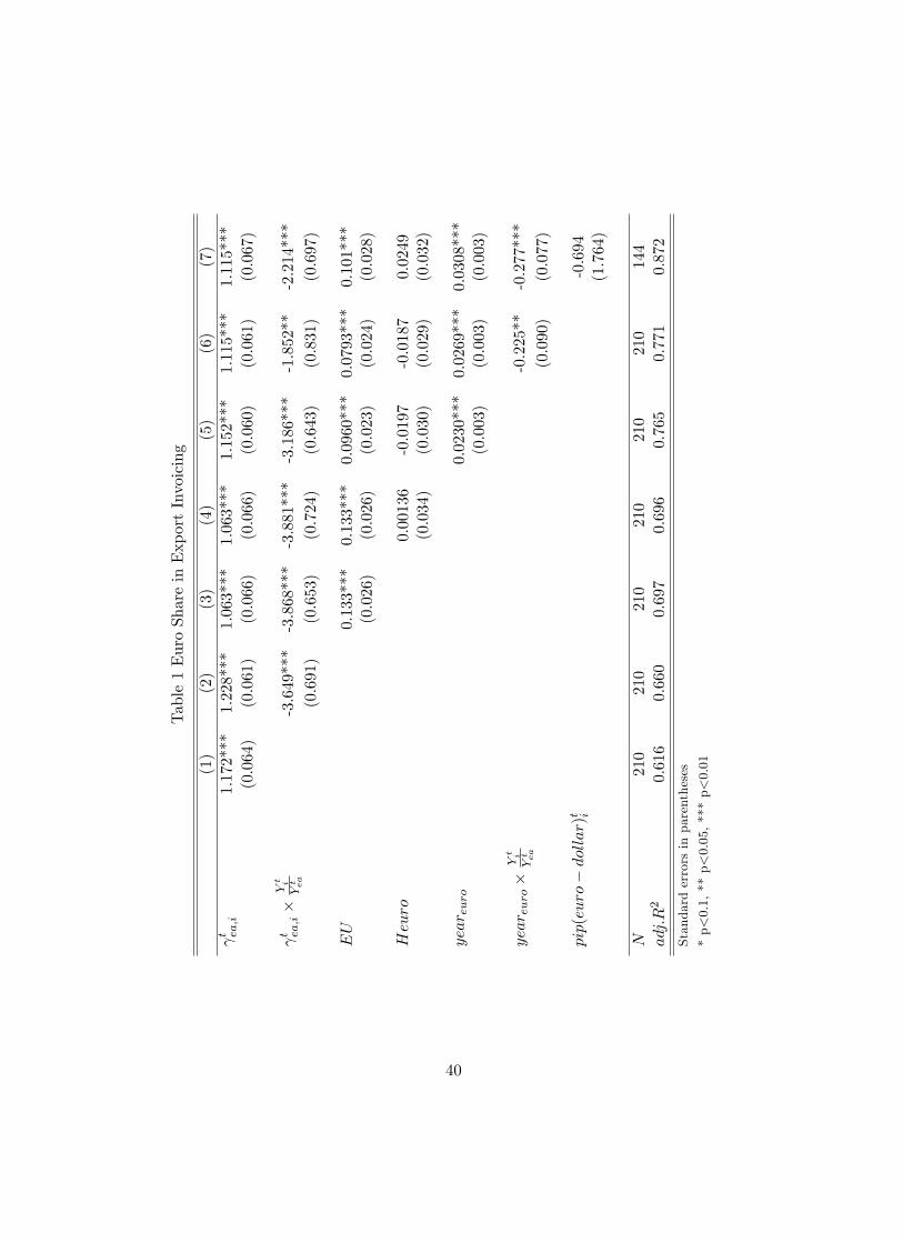
Table1EuroShareinExportInvoicing

(1)

(2)

(3)

(4)

(5)

(6)

(7)

t ea;i

1.172***

1.228***

1.063***

1.063***

1.152***

1.115***

1.115***

(0.064)

(0.061)

(0.066)

(0.066)

(0.060)

(0.061)

(0.067)

t ea;i�

Yt i

Yt ea

-3.649***

-3.868***

-3.881***

-3.186***

-1.852**

-2.214***

(0.691)

(0.653)

(0.724)

(0.643)

(0.831)

(0.697)

EU

0.133***

0.133***

0.0960***

0.0793***

0.101***

(0.026)

(0.026)

(0.023)

(0.024)

(0.028)

Heuro

0.00136

-0.0197

-0.0187

0.0249

(0.034)

(0.030)

(0.029)

(0.032)

year euro

0.0230***

0.0269***

0.0308***

(0.003)

(0.003)

(0.003)

year euro�

Yt i

Yt ea

-0.225**

-0.277***

(0.090)

(0.077)

pip(euro�dollar)t i

-0.694

(1.764)

N210

210

210

210

210

210

144

adj:R2

0.616

0.660

0.697

0.696

0.765

0.771

0.872

Standarderrorsinparentheses

*p<0.1,**p<0.05,***p<0.01

40

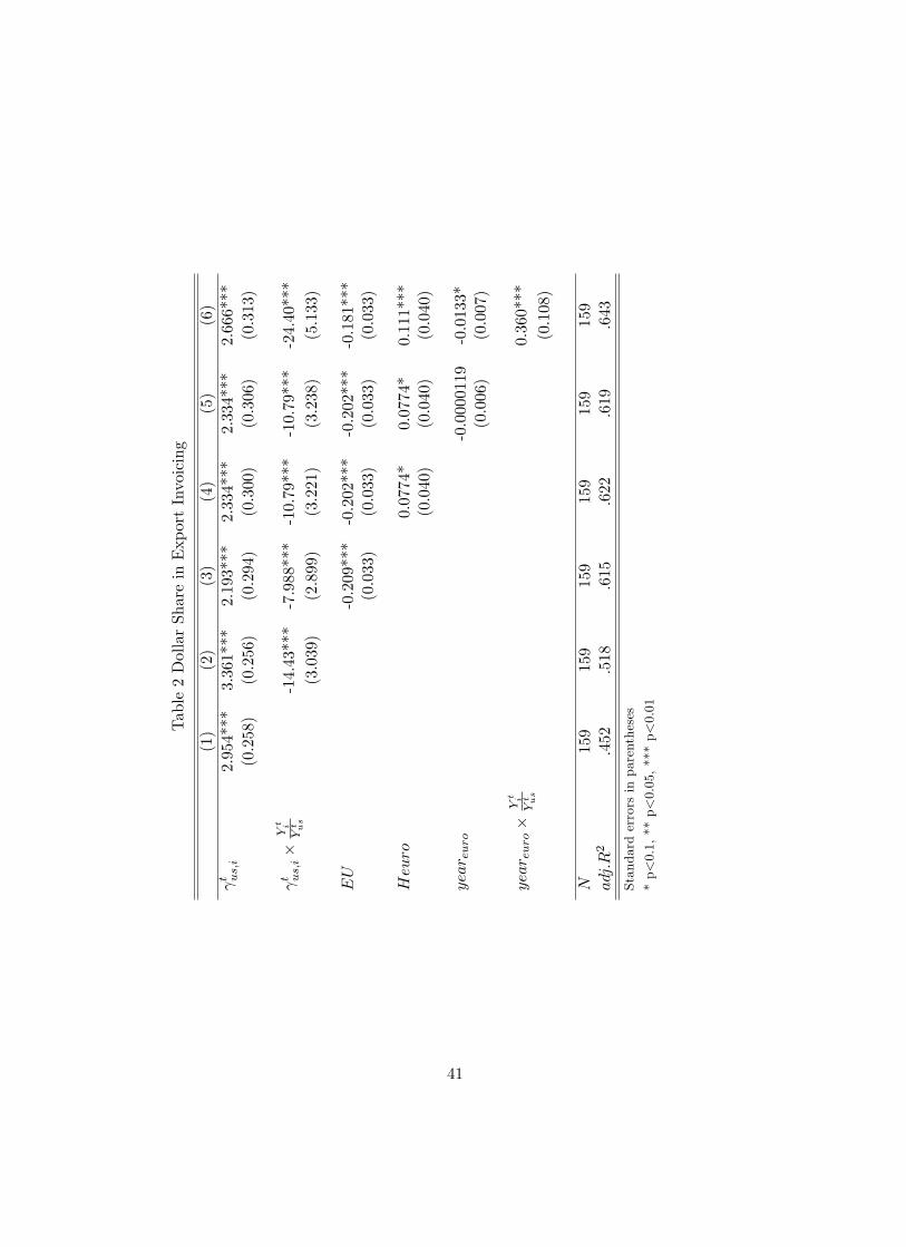
Table2DollarShareinExportInvoicing

(1)

(2)

(3)

(4)

(5)

(6)

t us;i

2.954***

3.361***

2.193***

2.334***

2.334***

2.666***

(0.258)

(0.256)

(0.294)

(0.300)

(0.306)

(0.313)

t us;i�

Yt i

Yt us

-14.43***

-7.988***

-10.79***

-10.79***

-24.40***

(3.039)

(2.899)

(3.221)

(3.238)

(5.133)

EU

-0.209***

-0.202***

-0.202***

-0.181***

(0.033)

(0.033)

(0.033)

(0.033)

Heuro

0.0774*

0.0774*

0.111***

(0.040)

(0.040)

(0.040)

year euro

-0.0000119

-0.0133*

(0.006)

(0.007)

year euro�

Yt i

Yt us

0.360***

(0.108)

N159

159

159

159

159

159

adj:R2

.452

.518

.615

.622

.619

.643

Standarderrorsinparentheses

*p<0.1,**p<0.05,***p<0.01

41

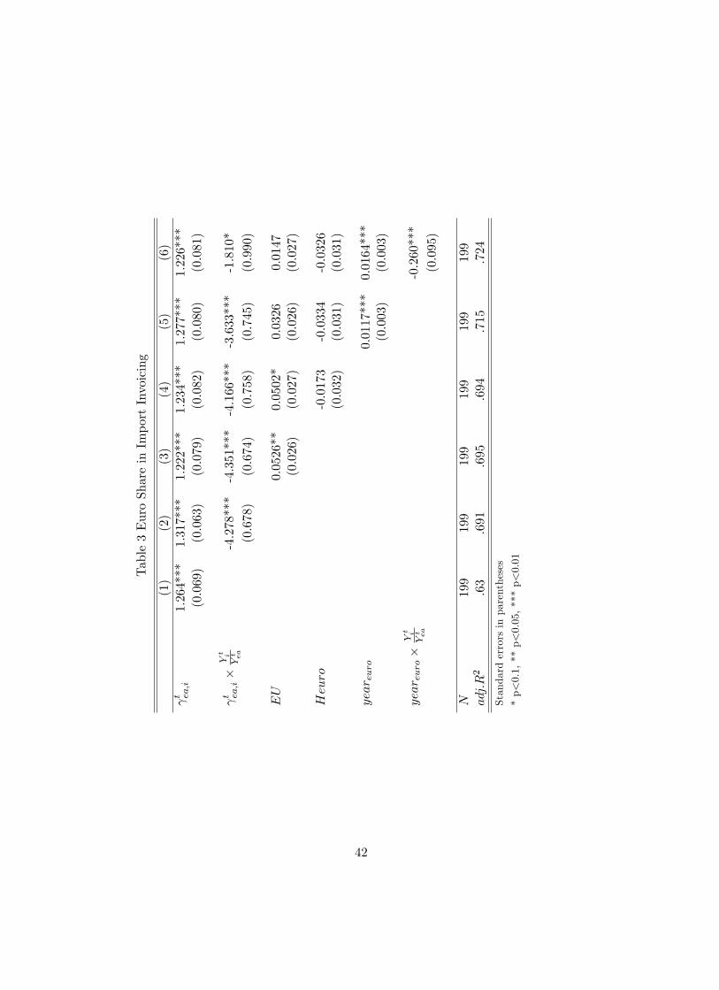
Table3EuroShareinImportInvoicing

(1)

(2)

(3)

(4)

(5)

(6)

t ea;i

1.264***

1.317***

1.222***

1.234***

1.277***

1.226***

(0.069)

(0.063)

(0.079)

(0.082)

(0.080)

(0.081)

t ea;i�

Yt i

Yt ea

-4.278***

-4.351***

-4.166***

-3.633***

-1.810*

(0.678)

(0.674)

(0.758)

(0.745)

(0.990)

EU

0.0526**

0.0502*

0.0326

0.0147

(0.026)

(0.027)

(0.026)

(0.027)

Heuro

-0.0173

-0.0334

-0.0326

(0.032)

(0.031)

(0.031)

year euro

0.0117***

0.0164***

(0.003)

(0.003)

year euro�

Yt i

Yt ea

-0.260***

(0.095)

N199

199

199

199

199

199

adj:R2

.63

.691

.695

.694

.715

.724

Standarderrorsinparentheses

*p<0.1,**p<0.05,***p<0.01

42

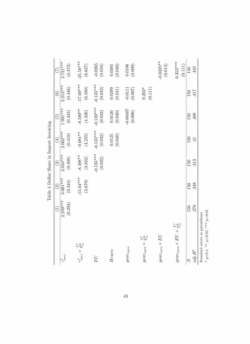
Table4DollarShareinImportInvoicing

(1)

(2)

(3)

(4)

(5)

(6)

(7)

t us;i

2.239***

3.061***

2.034***

2.062***

1.991***

2.213***

2.721***

(0.293)

(0.344)

(0.408)

(0.419)

(0.433)

(0.446)

(0.473)

t us;i�

Yt i

Yt us

-15.04***

-8.498**

-9.081**

-8.589**

-17.69***

-25.58***

(3.679)

(3.822)

(4.255)

(4.326)

(6.580)

(6.627)

EU

-0.135***

-0.135***

-0.139***

-0.135***

-0.0265

(0.032)

(0.032)

(0.033)

(0.033)

(0.058)

Heuro

0.0125

0.0120

0.0299

0.0385

(0.040)

(0.040)

(0.041)

(0.040)

year euro

-0.00407

-0.0111

0.0106

(0.006)

(0.007)

(0.009)

year euro�

Yt i

Yt us

0.202*

(0.111)

year euro�EU

-0.0325**

(0.013)

year euro�EU�

Yt i

Yt us

0.353***

(0.111)

N150

150

150

150

150

150

150

adj:R2

.278

.348

.413

.41

.408

.417

.445

Standarderrorsinparentheses

*p<0.1,**p<0.05,***p<0.01

43

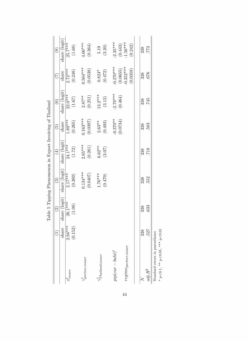
Table5TippingPhenomenoninExportInvoicingofThailand

(1)

(2)

(3)

(4)

(5)

(6)

(7)

(8)

share

share(logit)share(logit)share(logit)

share

share(logit)

share

share(logit)

xt issuer

2.94***

26.1***

2.17***

24.1***

1.89***

22.0***

2.72***

25.7***

(0.152)

(1.08)

(0.269)

(1.72)

(0.265)

(1.67)

(0.248)

(1.68)

t partner;issuer

0.134***

2.65***

0.163***

2.87**

0.564***

4.66***

(0.0407)

(0.261)

(0.0397)

(0.251)

(0.0538)

(0.364)

t Thailand;issuer

1.76***

6.62**

2.63**

13.2***

0.824*

5.19

(0.479)

(3.07)

(0.493)

(3.12)

(0.472)

(3.20)

pip(cur�baht)t

-0.370**

-2.79***

-0.270***

-2.35***

(0.0734)

(0.464)

(0.0655)

(0.443)

regime partner;issuer

-0.352***

-1.56***

(0.0358)

(0.242)

N338

338

338

338

338

338

338

338

adj:R2

.527

.633

.552

.718

.583

.745

.676

.773

Standarderrorsinparentheses

*p<0.1,**p<0.05,***p<0.01

44

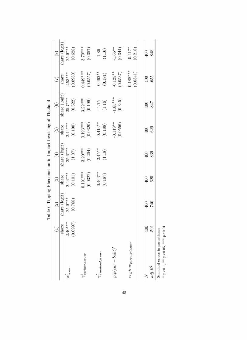
Table6TippingPhenomenoninImportInvoicingofThailand

(1)

(2)

(3)

(4)

(5)

(6)

(7)

(8)

share

share(logit)

share

share(logit)

share

share(logit)

share

share(logit)

xt issuer

2.40***

25.9***

2.44***

25.6***

2.44***

25.7***

2.53***

25.9***

(0.0997)

(0.768)

(0.101)

(1.07)

(0.100)

(0.622)

(0.0980)

(0.628)

t partner;issuer

0.191***

3.20***

0.193***

3.22***

0.449***

3.79***

(0.0322)

(0.204)

(0.0320)

(0.199)

(0.0557)

(0.357)

t Thailand;issuer

-0.463**

-2.45**

-0.413**

-1.75

-0.462**

-1.86

(0.187)

(1.18)

(0.188)

(1.16)

(0.181)

(1.16)

pip(cur�baht)t

-0.119**

-1.65***

-0.125**

-1.66**

(0.0556)

(0.345)

(0.0537)

(0.344)

regime partner;issuer

-0.188***

-0.417*

(0.0341)

(0.218)

N400

400

400

400

400

400

400

400

adj:R2

.591

.740

.625

.839

.629

.847

.655

.848

Standarderrorsinparentheses

*p<0.1,**p<0.05,***p<0.01

45

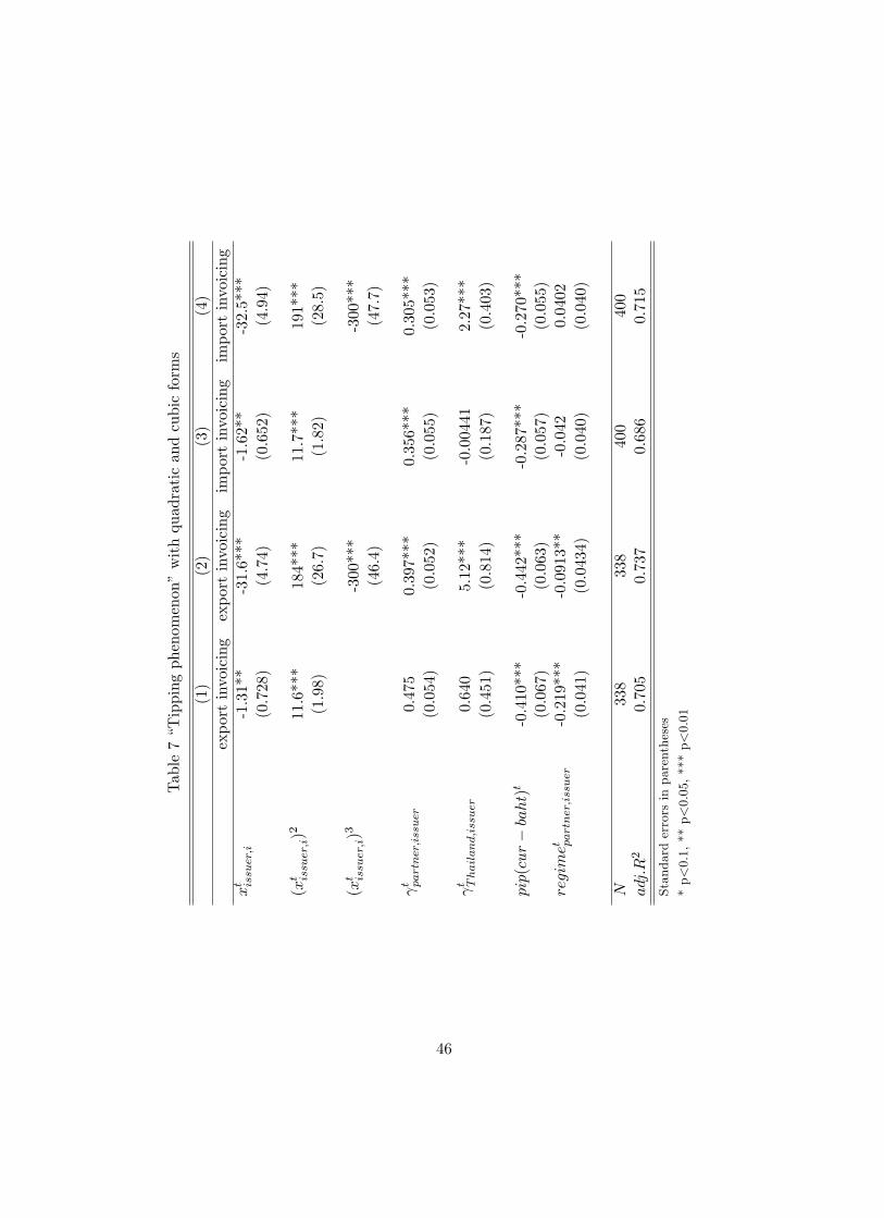
Table7�Tippingphenomenon�withquadraticandcubicforms

(1)

(2)

(3)

(4)

exportinvoicing

exportinvoicing

importinvoicing

importinvoicing

xt issuer;i

-1.31**

-31.6***

-1.62**

-32.5***

(0.728)

(4.74)

(0.652)

(4.94)

(xt issuer;i)2

11.6***

184***

11.7***

191***

(1.98)

(26.7)

(1.82)

(28.5)

(xt issuer;i)3

-300***

-300***

(46.4)

(47.7)

t partner;issuer

0.475

0.397***

0.356***

0.305***

(0.054)

(0.052)

(0.055)

(0.053)

t Thailand;issuer

0.640

5.12***

-0.00441

2.27***

(0.451)

(0.814)

(0.187)

(0.403)

pip(cur�baht)t

-0.410***

-0.442***

-0.287***

-0.270***

(0.067)

(0.063)

(0.057)

(0.055)

regimet partner;issuer

-0.219***

-0.0913**

-0.042

0.0402

(0.041)

(0.0434)

(0.040)

(0.040)

N338

338

400

400

adj:R2

0.705

0.737

0.686

0.715

Standarderrorsinparentheses

*p<0.1,**p<0.05,***p<0.01

46

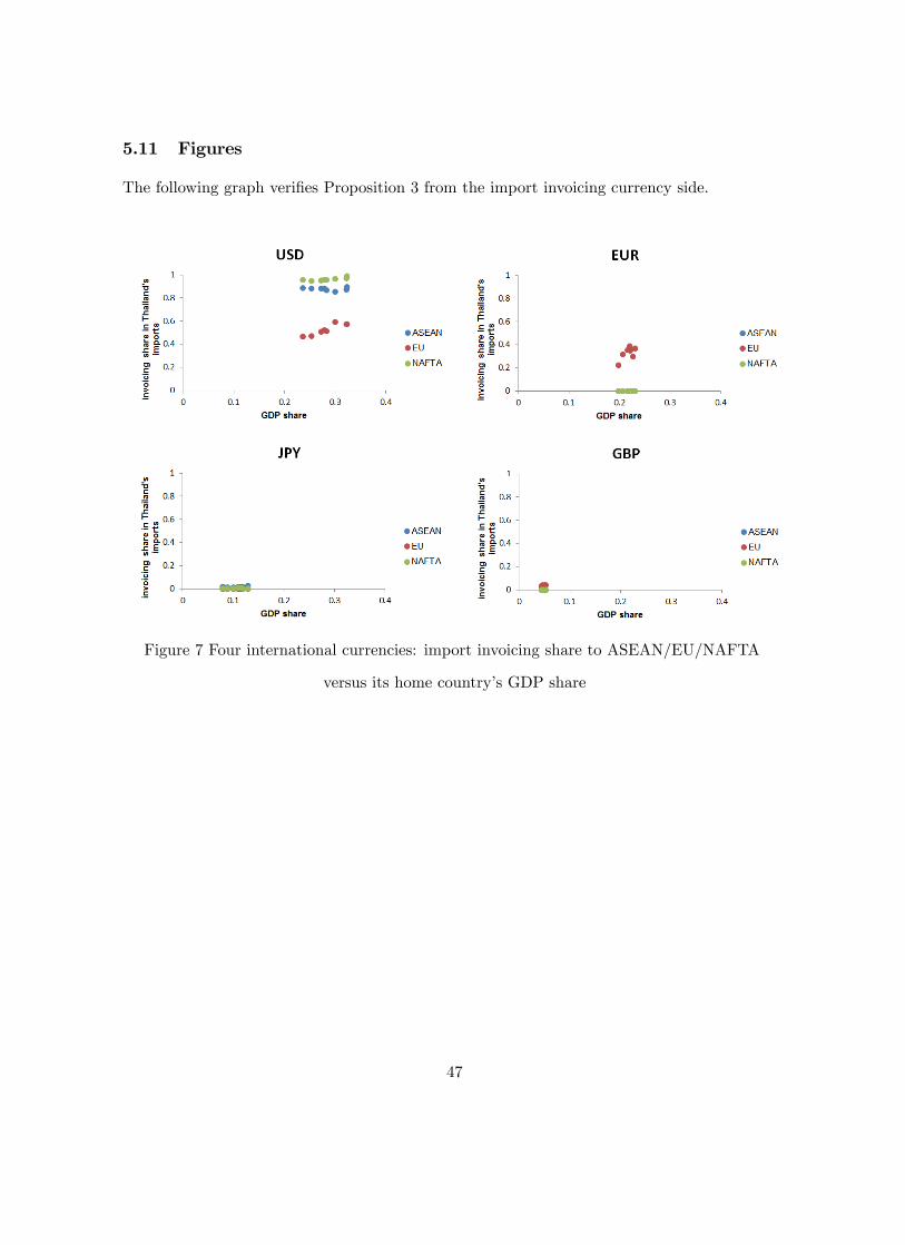
5.11 Figures

The following graph veri�es Proposition 3 from the import invoicing currency side.

Figure 7 Four international currencies: import invoicing share to ASEAN/EU/NAFTA

versus its home country�s GDP share

47