The elementary evolutionary operator

1. Hardy-Weinberg Law

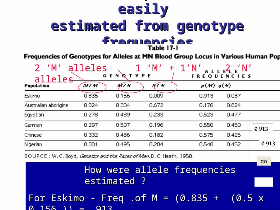
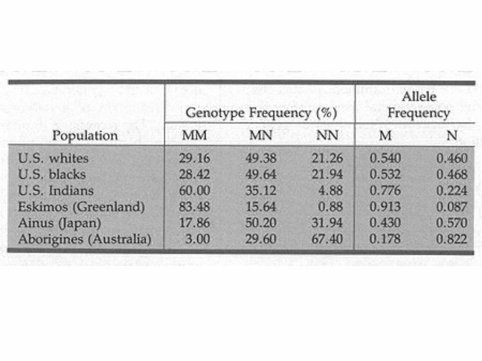
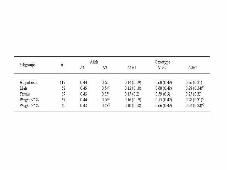
Allele frequencies are easily Allele frequencies are easily estimated from genotype frequenciesestimated from genotype frequencies

How were allele frequencies estimated ?How were allele frequencies estimated ?

For Eskimo - Freq .of M = (0.835 + (0.5 x 0.156 )) = .913For Eskimo - Freq .of M = (0.835 + (0.5 x 0.156 )) = .913

Freq. of N = (0.009 + .(0.5 x 0.156 )) = .087Freq. of N = (0.009 + .(0.5 x 0.156 )) = .087

2 ‘M’ alleles 1 ‘M’ + 1’N’ 2 ‘N’ alleles

go

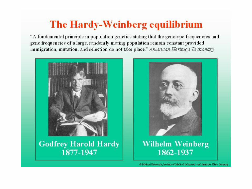
Why Hardy-Weinberg Law?

Hardy-Weinberg Law is a dynamical effect

evolutionary operator

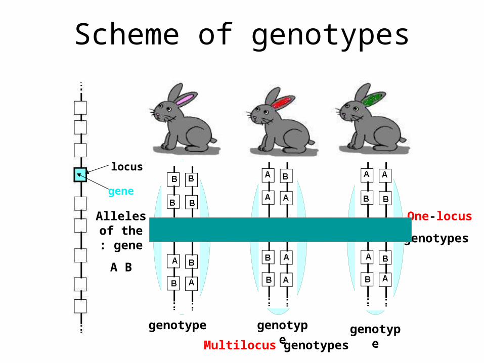
Scheme of genotypes

locus

gene

Alleles of the gene:

A B

genotype genotype

One-locus

genotypes

Multilocus genotypesgenotype

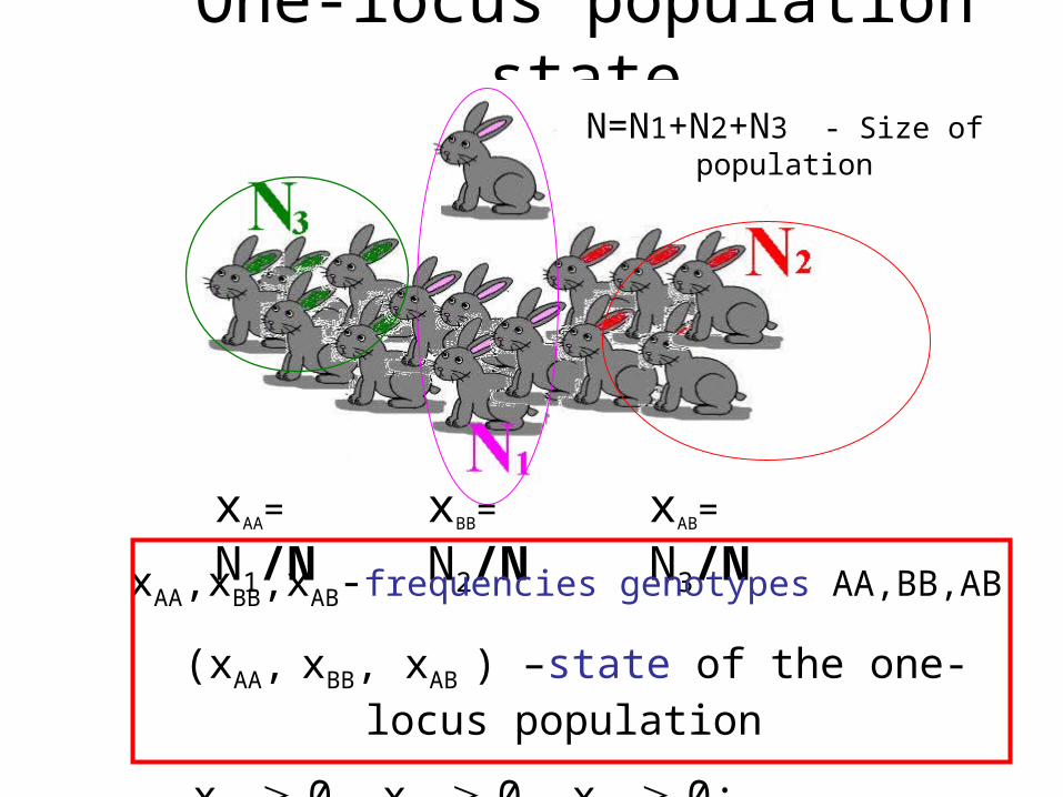
One-locus population stateN=N1+N2+N3 - Size of population

xAA= N1/N xBB= N2/N xAB= N3/N

xAA,xBB,xAB-frequencies genotypes AA,BB,AB

(xAA, xBB, xAB ) –state of the one-locus population

xAA 0, xBB 0, xAB 0; xAA+xBB+xAB=1.

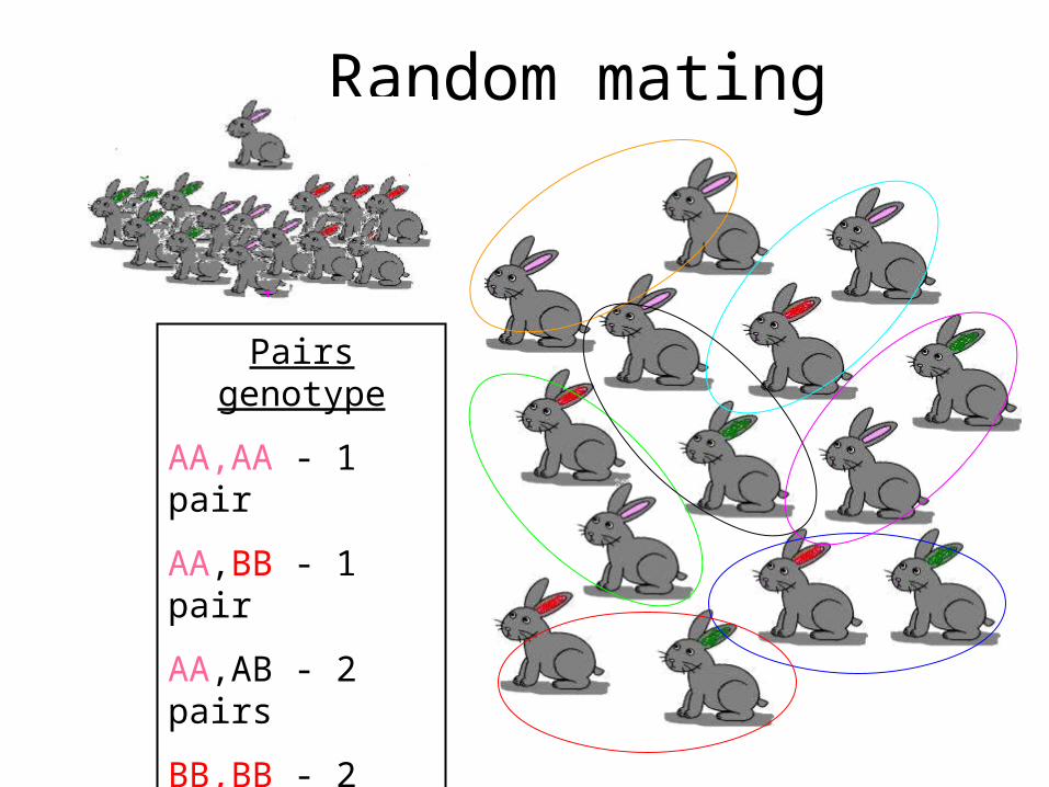
Random mating

Pairs genotype

AA,AA - 1 pair

AA,BB - 1 pair

AA,AB - 2 pairs

BB,BB - 2 pairs

BB,AB - 2 pairs

AB,AB - 0

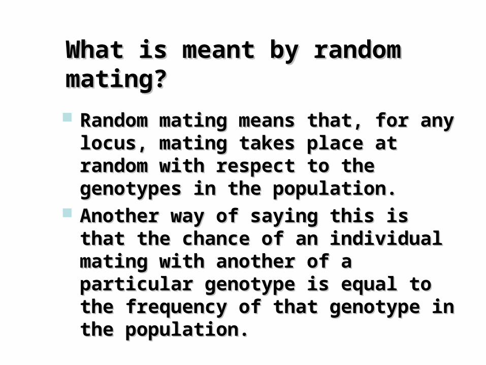
What is meant by random What is meant by random mating?mating?

Random mating means that, for any Random mating means that, for any locus, mating takes place at locus, mating takes place at random with respect to the random with respect to the genotypes in the population.genotypes in the population.

Another way of saying this is that Another way of saying this is that the chance of an individual mating the chance of an individual mating with another of a particular with another of a particular genotype is equal to the frequency genotype is equal to the frequency of that genotype in the population.of that genotype in the population.

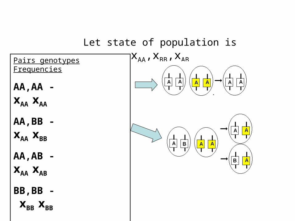
Pairs genotypes Frequencies

AA,AA - xAA xAA

AA,BB - xAA xBB

AA,AB - xAA xAB

BB,BB - xBB xBB

BB,AB - xBB xAB

AB,AB - xAB xAB

Let state of population is xAA,xBB,xAB

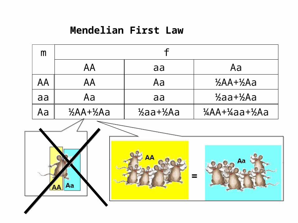
f

aaAA Aa

m

AA

Aa

Aa

aa

½AA+½Aa

½aa+½Aa

½aa+½Aa ¼AA+¼aa+½Aa

AA

aa

Aa

Mendelian First Law

½AA+½Aa

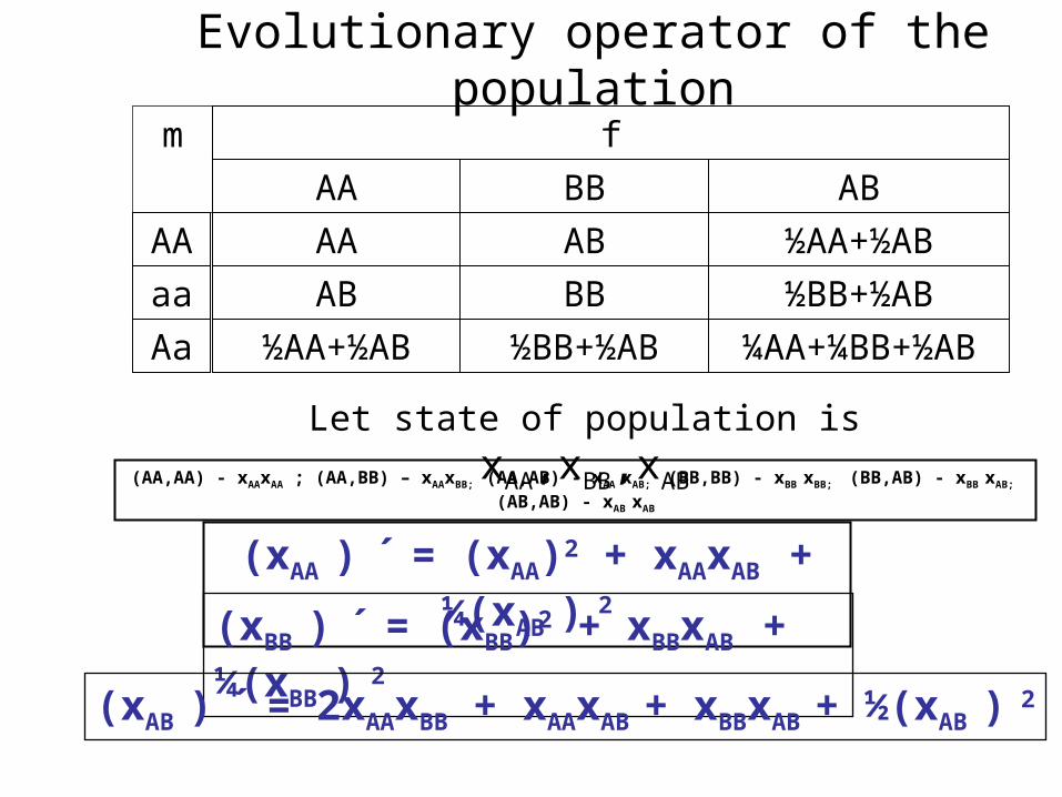
Evolutionary operator of the population

f

BBAA AB

m

AA

AB

AB

BB

½AA+½AB

½BB+½AB

½BB+½AB ¼AA+¼BB+½AB

AA

aa

Aa ½AA+½AB

Let state of population is xAA,xBB,xAB

(AA,AA) - xAAxAA ; (AA,BB) – xAAxBB; (AA,AB) - xAA xAB; (BB,BB) - xBB xBB; (BB,AB) - xBB xAB; (AB,AB) - xAB xAB

(xAA ) ´ = (xAA)2 + xAAxAB + ¼(xAB ) 2

(xBB ) ´ = (xBB)2 + xBBxAB + ¼(xBB ) 2

(xAB ) ´ = 2xAAxBB + xAAxAB + xBBxAB + ½(xAB ) 2

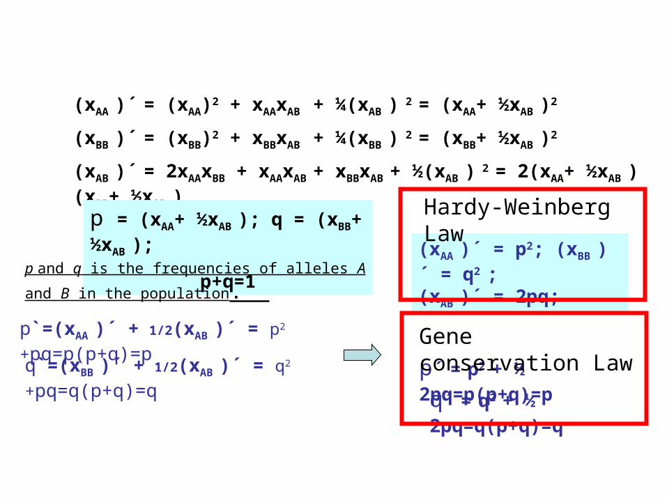
(xAA )´ = (xAA)2 + xAAxAB + ¼(xAB ) 2 = (xAA+ ½xAB )2

(xBB )´ = (xBB)2 + xBBxAB + ¼(xBB ) 2 = (xBB+ ½xAB )2

(xAB )´ = 2xAAxBB + xAAxAB + xBBxAB + ½(xAB ) 2 = 2(xAA+ ½xAB )(xBB+ ½xAB )

p = (xAA+ ½xAB ); q = (xBB+ ½xAB );

p+q=1p and q is the frequencies of alleles A and B in the population.

(xAA )´ = p2; (xBB ) ´ = q2 ;(xAB )´ = 2pq;

p´ = p2 + ½ 2pq=p(p+q)=p

q´ = q2 + ½ 2pq=q(p+q)=q

Gene conservation Law

Hardy-Weinberg Law

p`=(xAA )´ + 1/2(xAB )´ = p2 +pq=p(p+q)=p

q`=(xBB )´ + 1/2(xAB )´ = q2 +pq=q(p+q)=q

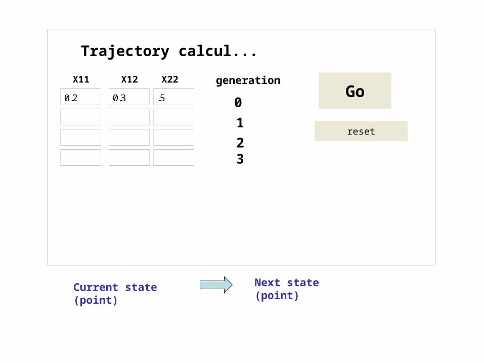
Trajectory calculator

X11 X12 X22 generation

0Go

reset1

23

Current state (point) Next state (point)

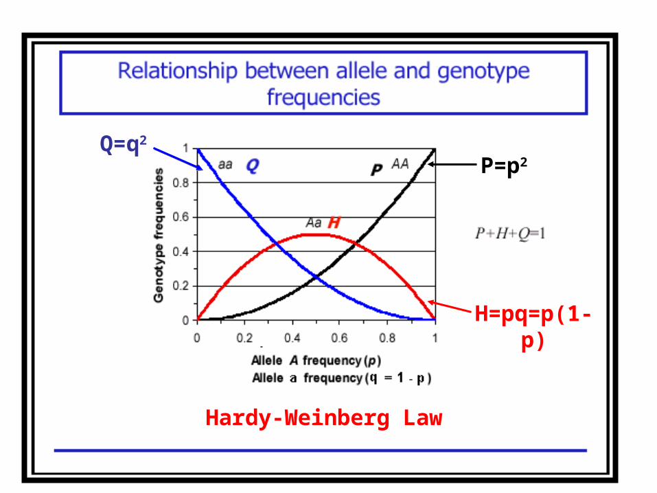
P=p2Q=q2

H=pq=p(1-p)

Hardy-Weinberg Law

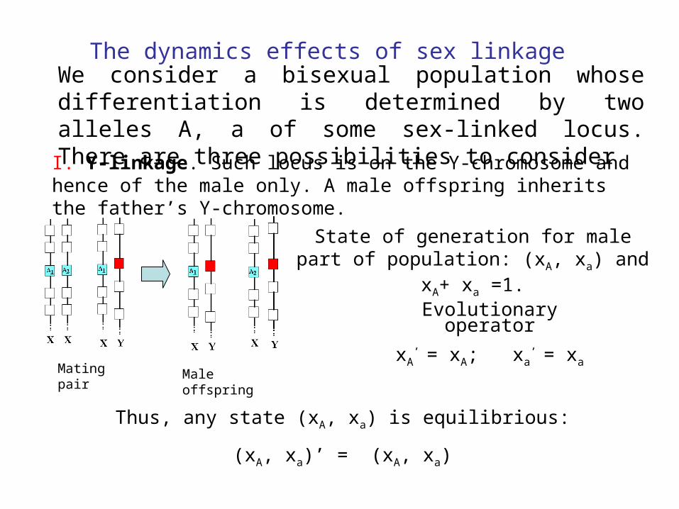
The dynamics effects of sex linkage We consider a bisexual population whose differentiation is determined by two alleles A, a of some sex-linked locus. There are three possibilities to consider

I. Y-linkage. Such locus is on the Y-chromosome and hence of the male only. A male offspring inherits the father’s Y-chromosome.

Mating pair Male offspring

Thus, any state (xA, xa) is equilibrious:

(xA, xa)’ = (xA, xa)

State of generation for male part of population: (xA, xa) and xA+ xa =1.

Evolutionary operator

xA’ = xA; xa

’ = xa

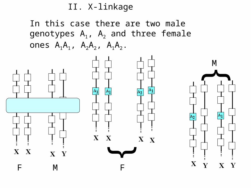
II. X-linkage

}

}

F

M

In this case there are two male genotypes A1, A2 and three female ones A1A1, A2A2, A1A2.

F M

f

A2 A2A1A1 A1 A2mA1

A1

A2

A2

½A1+½ A2

½A1+½ A2

A1

A2

f

A2 A2A1A1 A1 A2mA1A1

A1 A2

A1 A2

A2 A2

½A1A1+½A1 A2

½ A2 A2 +½A1 A2

A1

A2

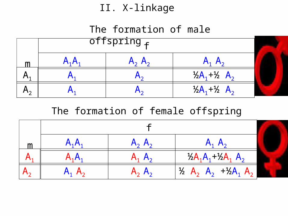
The formation of male offspring

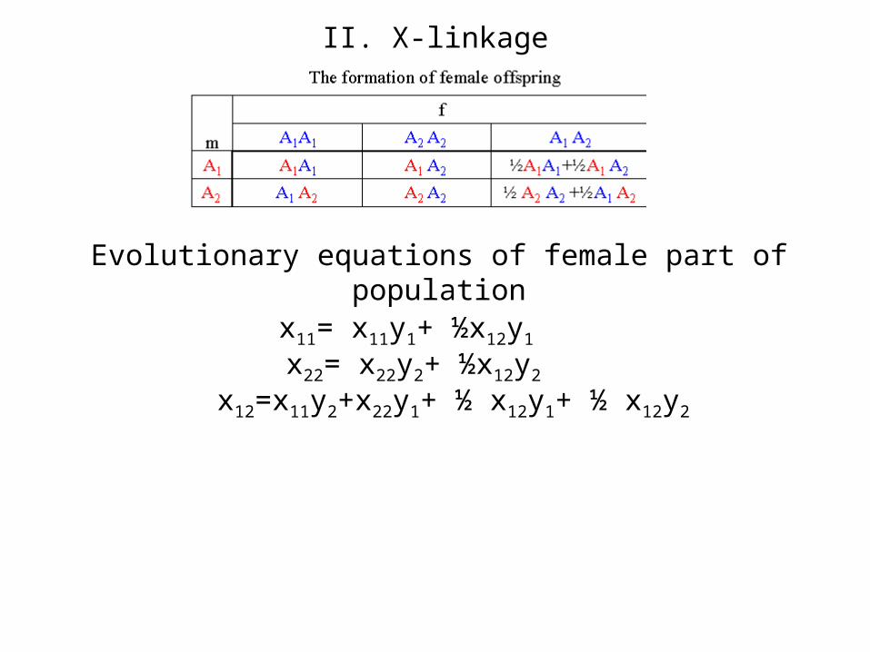
The formation of female offspring

II. X-linkage

II. X-linkage

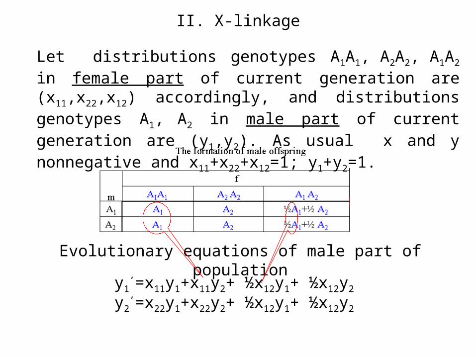
Let distributions genotypes A1A1, A2A2, A1A2 in female part of current generation are (x11,x22,x12) accordingly, and distributions genotypes A1, A2 in male part of current generation are (y1,y2). As usual x and y nonnegative and x11+x22+x12=1; y1+y2=1.

Evolutionary equations of male part of population

y1’=x11y1+x11y2+ ½x12y1+ ½x12y2

y2’=x22y1+x22y2+ ½x12y1+ ½x12y2

II. X-linkage

Evolutionary equations of female part of population

x11= x11y1+ ½x12y1

x22= x22y2+ ½x12y2

x12=x11y2+x22y1+ ½ x12y1+ ½ x12y2

II. X-linkage

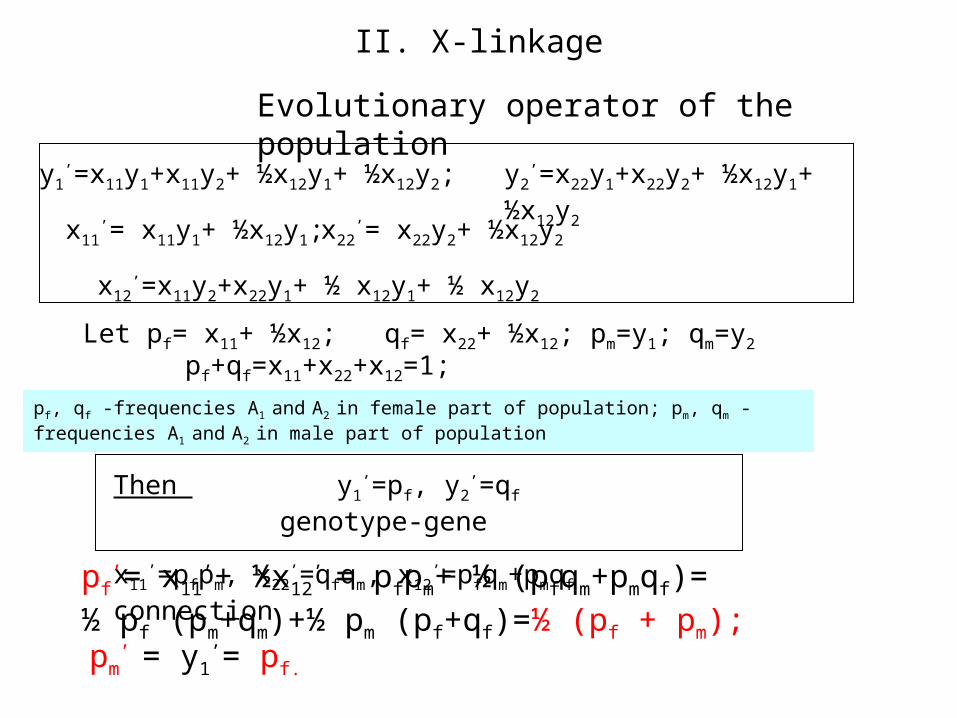
Evolutionary operator of the population

y1’=x11y1+x11y2+ ½x12y1+ ½x12y2; y2

’=x22y1+x22y2+ ½x12y1+ ½x12y2

x11’= x11y1+ ½x12y1; x22

’= x22y2+ ½x12y2

x12’=x11y2+x22y1+ ½ x12y1+ ½ x12y2

Let pf= x11+ ½x12; qf= x22+ ½x12; pm=y1; qm=y2

Then y1’=pf, y2

’=qf genotype-gene

x11’=pfpm, x22

’=qfqm, x12’=pfqm+pmqf connection

pf’= x11

’+ ½x12’ = pfpm+ ½ (pfqm+pmqf)=

½ pf (pm+qm)+½ pm (pf+qf)=½ (pf + pm);

pf+qf=x11+x22+x12=1; pm+qm=y1+y2=1

pm’ = y1

’= pf.

pf, qf -frequencies A1 and A2 in female part of population; pm, qm -frequencies A1 and A2 in male part of population

II. X-linkage

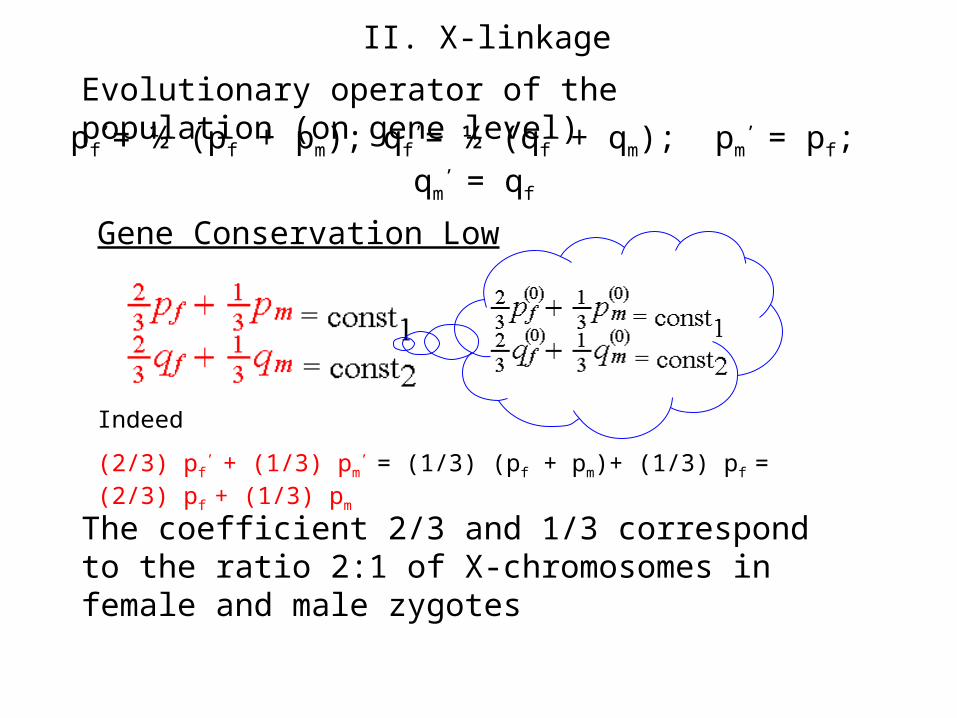
Evolutionary operator of the population (on gene level)

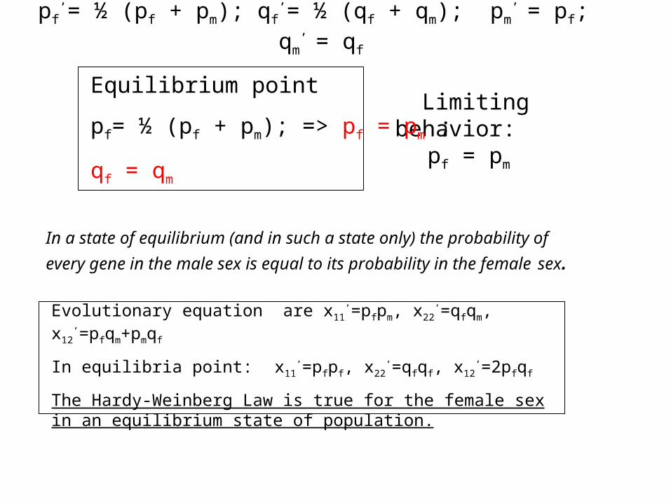
pf’= ½ (pf + pm); qf

’= ½ (qf + qm); pm’ = pf; qm

’ = qf

Gene Conservation Low

Indeed

(2/3) pf’ + (1/3) pm

’ = (1/3) (pf + pm)+ (1/3) pf = (2/3) pf + (1/3) pm

The coefficient 2/3 and 1/3 correspond to the ratio 2:1 of X-chromosomes in female and male zygotes

pf’= ½ (pf + pm); qf

’= ½ (qf + qm); pm’ = pf; qm

’ = qf

Limiting behavior: pf = pm

Equilibrium point

pf= ½ (pf + pm); => pf = pm ;

qf = qm

In a state of equilibrium (and in such a state only) the probability of every

gene in the male sex is equal to its probability in the female sex.

Evolutionary equation are x11’=pfpm, x22

’=qfqm, x12’=pfqm+pmqf

In equilibria point: x11’=pfpf, x22

’=qfqf, x12’=2pfqf

The Hardy-Weinberg Law is true for the female sex in an equilibrium state of population.

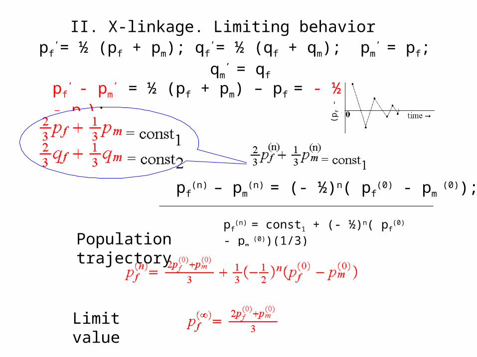
II. X-linkage. Limiting behavior

pf’ - pm

’ = ½ (pf + pm) – pf = - ½ (pf - pm);

pf’= ½ (pf + pm); qf

’= ½ (qf + qm); pm’ = pf; qm

’ = qf

(pf -

pm)

pf(n) – pm

(n) = (- ½)n( pf(0) - pm

(0));

pf(n) = const1 + (- ½)n( pf

(0) - pm (0))(1/3)

Population trajectory

Limit value

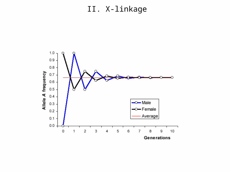
II. X-linkage

Limit value

Population trajectory

Since the condition pf = pm is nessesary and sufficiently for an equilibrium then difference (pf - pm) may be regarded as the measure of disequilibrium of state of the population. The modulus of measure of disequilibrium is halved for one generation, and its sing alternates, I.e. an excess of genes is pumped from one sex to another.

If (pf - pm) 0 in start point then (pf - pm) 0 along the trajectory.Therefore, the population under consideration is non-stationary.

II. X-linkage