The Elastic Behavior of Plagioclase Feldspar at High Pressure

Eleda M. Johnson

Thesis submitted to the faculty of the Virginia Polytechnic Institute and State University in partial fulfillment of the requirements for the degree of

Master of Science

In Geosciences

Dr. Ross Angel, Chair Dr. Nancy Ross

Dr. Michael Carpenter

December 7, 2007 Blacksburg, Va

Keywords: plagioclase, pressure, elasticity, equation of state, bulk modulus, unit-cell parameters,

X-ray diffraction

The Elastic Behavior of Plagioclase Feldspars at High Pressure

Eleda M. Johnson

Abstract Feldspars are one of the archetypical families of framework silicates. They not only comprise

around 60% volumetrically of the Earth’s crust, but are among some of the most structurally

complicated minerals. Investigation into the structural behavior of various intermediate

plagioclases at pressure has been undertaken with the intent of categorizing the elastic behavior

with pressure across the solid solution series and establishing a conceptual model to characterize

feldspar compression.

Complex behavior has been observed in the Equation of State for plagioclase feldspars in excess

of 3 GPa, including an anomalous softening of ordered albite in excess of 8.4 GPa (Benusa et al

2005: Am Min 90:1115-1120). This softening was not observed in the EoS for the more

intermediate plagioclase compositions containing between 20 and 40 mol% of end-member

anorthite. The calculated elastic compliance tensor sums at room pressure show a general

stiffening with increasing anorthite component, small elastic changes at the C-1 to I-1 transition,

and a dominantly first-order response at the P-1 to I-1 transition near end-member anorthite.

The crystal structure of An37 plagioclase was determined by single-crystal X-ray diffraction.

The compression mechanisms in An37 are similar to those in albite at lower pressures. The

softening in albite at higher pressures is therefore attributed to the structural shearing in albite

that is absent in An37 plagioclase up to 9.5 GPa.

Grant Information The research reported in this thesis was supported in part by NSF grant EAR0408460 to Dr.

Nancy Ross and Dr. Ross Angel.

Author’s Acknowledgements Much thanks to Dr. Ross Angel for his vast amount of input into this research.

.

Dr. Michael Brown kindly donated three of the samples used in this research, while Dr. Michael

Carpenter supplied the remaining samples.

The An37A/B analyses were done mainly under the direct guidance of Dr. Fabrizio Nestola.

Much of this research was supported by TA stipends through the Department of Geosciences at

Virginia Tech.

Many thanks also to Dr. Jing Zhou, Dr. Carla Slebodnick, Dr. Nancy Ross, Dr. Bob Bodnar,

Charles Farley, and the VTX group and fellow graduate students.

iii

Table of Contents Abstract ........................................................................................................................................... ii Grant Information .......................................................................................................................... iii Author’s Acknowledgements......................................................................................................... iii List of Figures ................................................................................................................................. v List of Tables ................................................................................................................................. vi Chapter 1 Introduction................................................................................................................. 1

1.1 Chapter Introduction ....................................................................................................... 1 1.2 Feldspar Structure ........................................................................................................... 1 1.3 Thermodynamics........................................................................................................... 10

Chapter 2 Experimental Methods .............................................................................................. 13 2.1 Chapter Introduction ..................................................................................................... 13 2.2 X-ray diffraction ........................................................................................................... 13 2.3 Diamond Anvil Cell...................................................................................................... 15 2.4 Structure analysis .......................................................................................................... 21 2.5 Elasticity ....................................................................................................................... 26 2.6 Equation of State........................................................................................................... 31

Chapter 3 Results....................................................................................................................... 35 3.1 Chapter Introduction ..................................................................................................... 35 3.2 Unit-cell parameters...................................................................................................... 35 3.3 Equations of State ......................................................................................................... 49 3.4 Compliance Tensor Sums ............................................................................................. 51 3.5 Structure........................................................................................................................ 54

Chapter 4 Discussion................................................................................................................. 55 4.1 Chapter Introduction ..................................................................................................... 55 4.2 Cell Parameter Trends................................................................................................... 55 4.3 f-F Plot Description....................................................................................................... 56 4.4 Bulk Modulus................................................................................................................ 58 4.5 P-1 – I-1 Phase Transition............................................................................................. 60 4.6 Structure: An37 at high pressure................................................................................... 67 4.7 Strain Tensor................................................................................................................. 73 4.8 Summary ....................................................................................................................... 80

References..................................................................................................................................... 82 Appendix A Unit-cell Parameter Data....................................................................................... 88 Appendix B Strain Tensor Data ................................................................................................ 99 Appendix C Structure Data ..................................................................................................... 110

iv

List of Figures Figure 1.1 Aristotype feldspar structure: ........................................................................................ 2 Figure 1.2 Schematic K-feldspar phase diagram ............................................................................ 8 Figure 1.3 Plagioclase phase diagram............................................................................................. 9 Figure 2.1 DAC pressure cartoon ................................................................................................. 15 Figure 2.2 DAC cross-section....................................................................................................... 17 Figure 2.3 ETH-DAC schematic................................................................................................... 18 Figure 2.4 Xcalibur-1 and Xcalibure-2 pictures ........................................................................... 22 Figure 2.5 Huber picture ............................................................................................................... 25 Figure 2.6 An37 f-F plot ............................................................................................................... 34 Figure 3.1 An00 unit-cell parameters ........................................................................................... 37 Figure 3.2 An20 unit-cell parameters ........................................................................................... 38 Figure 3.3 An36 unit-cell parameters ........................................................................................... 39 Figure 3.4 An45 unit-cell parameters ........................................................................................... 40 Figure 3.5 An68 unit-cell parameters ........................................................................................... 41 Figure 3.6 An77 unit-cell parameters ........................................................................................... 42 Figure 3.7 An89 unit-cell parameters ........................................................................................... 43 Figure 3.8 An37X2 unit-cell parameters ...................................................................................... 45 Figure 3.9 An50 unit-cell parameters ........................................................................................... 46 Figure 3.10 An60 unit-cell parameters ......................................................................................... 47 Figure 3.11 An96 unit-cell parameters ......................................................................................... 48 Figure 3.12 f-F plot for all compositions ...................................................................................... 50 Figure 3.12 An37X2 unit-cell parameters with compliance tensor sums..................................... 52 Figure 4.1 b vs. c plot.................................................................................................................... 56 Figure 4.2 Room pressure Bulk Modulus vs. composition........................................................... 59 Figure 4.3 Bulk Modulus vs. composition with pressure ............................................................. 60 Figure 4.4 Spontaneous strain....................................................................................................... 63 Figure 4.5 Scalar spontaneous strain ............................................................................................ 65 Figure 4.6 Bulk Modulus vs. QOD

2 ............................................................................................... 67 Figure 4.7 An37 M-O bond distances........................................................................................... 70 Figure 4.8 An00 and An37 T-O-T bond distances ....................................................................... 72 Figure 4.9 K, K’ vs. pressure for An00 and An37........................................................................ 73 Figure 4.10 An00 principal strain axes orientation....................................................................... 74 Figure 4.11 Plagioclase principal strain orientation ..................................................................... 75 Figure 4.12 An89 and An96 compliance tensor sums .................................................................. 77 Figure 4.13 Zero-pressure compliance tensor sums vs. composition ........................................... 78 Figure 4.14 Scaled zero-pressure compliance tensor sums vs. composition ................................ 80

v

List of Tables Table 1.1 Feldspar nomenclature.................................................................................................... 4 Table 3.1 Plagioclase sample details ............................................................................................ 36 Table 3.2 EoS fit parameters......................................................................................................... 49 Table 4.1 Order parameters........................................................................................................... 66

vi

Chapter 1 Introduction

1.1 Chapter Introduction Feldspars are some of the most abundant minerals found in the Earth’s crust, and have a long

history of scientific investigation into their physical properties and structure. One of the few

areas of research in regards to feldspars which has benefited in recent years from advances in

experimental methods is the characterization of their behavior with pressure. This thesis looks at

the behavior at high pressure of a suite of plagioclase feldspars encompassing the full solid-

solution series and their elastic responses in order to try and identify the underlying structural

mechanisms and to formulate a conceptual framework for evaluating feldspar behavior with

pressure. First a brief introduction of feldspars will be given. This is followed by a description of

the methods used in this investigation, an outline of the results, and a discussion of what

conclusions can be drawn from those results in the context of what has previously been

determined in the literature.

1.2 Feldspar Structure

Feldspars have the general formula of AT4O8, where ‘T’ refers to the framework structure of

corner-sharing alumino-silicate tetrahedra and ‘A’ refers to the charge-balanced larger interstitial

cation sites. In general T sites are occupied by Si and Al, while the A sites are occupied

dominantly by Na+, K+, or Ca2+ as well as Sr2+ or Ba2+, where a ratio of 1:3::Al:Si balances out

structures with monovalent cations and a ratio of 2:2::Al:Si balances out structures with divalent

cations. Other less common elemental compositions are known both naturally and synthetically,

but will not be discussed here. Instead, the following will discuss the natural compositional range

of KxNayCa1-(x+y)Al2-(x+y)Si2+(x+y)O8 (or OrxAbyAn1-(x+y) if referenced to the end member

components), outlining the essential topologic architecture of the feldspar family starting with

the composition of the highest structural symmetry and branching out via the processes

governing the phase relations to compositions of lower symmetry (Ribbe 1983).

1

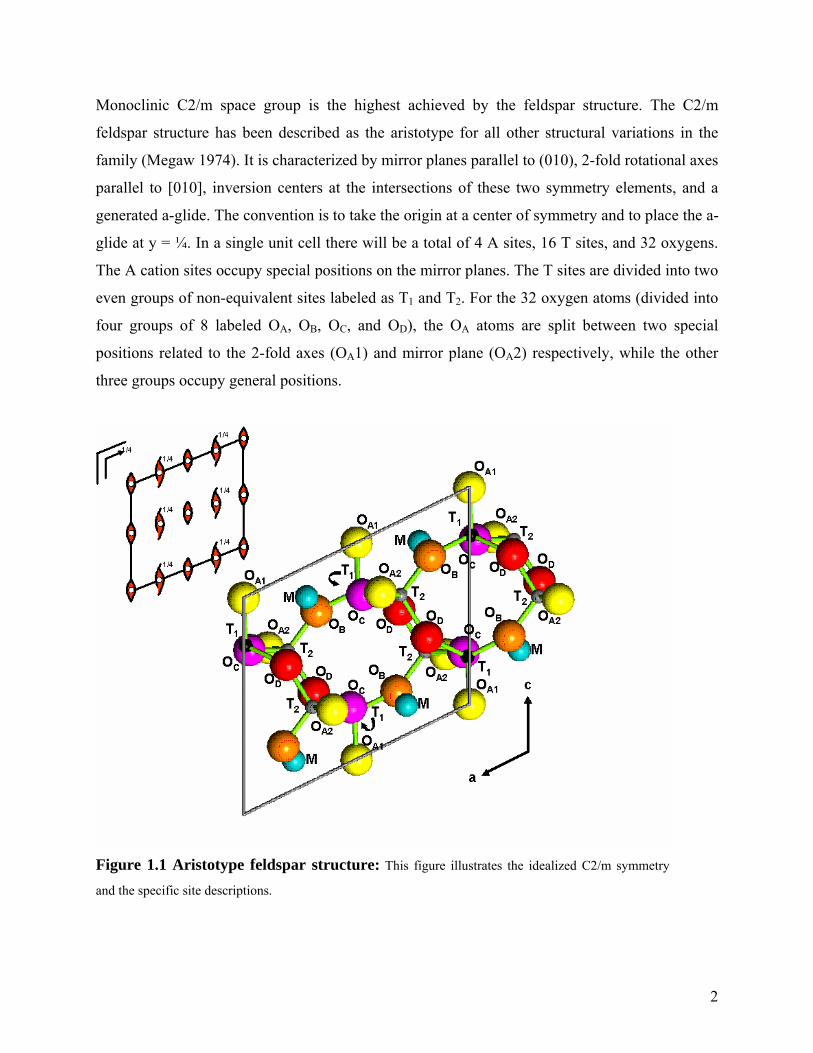
Monoclinic C2/m space group is the highest achieved by the feldspar structure. The C2/m

feldspar structure has been described as the aristotype for all other structural variations in the

family (Megaw 1974). It is characterized by mirror planes parallel to (010), 2-fold rotational axes

parallel to [010], inversion centers at the intersections of these two symmetry elements, and a

generated a-glide. The convention is to take the origin at a center of symmetry and to place the a-

glide at y = ¼. In a single unit cell there will be a total of 4 A sites, 16 T sites, and 32 oxygens.

The A cation sites occupy special positions on the mirror planes. The T sites are divided into two

even groups of non-equivalent sites labeled as T1 and T2. For the 32 oxygen atoms (divided into

four groups of 8 labeled OA, OB, OC, and OD), the OA atoms are split between two special

positions related to the 2-fold axes (OA1) and mirror plane (OA2) respectively, while the other

three groups occupy general positions.

Figure 1.1 Aristotype feldspar structure: This figure illustrates the idealized C2/m symmetry

and the specific site descriptions.

2

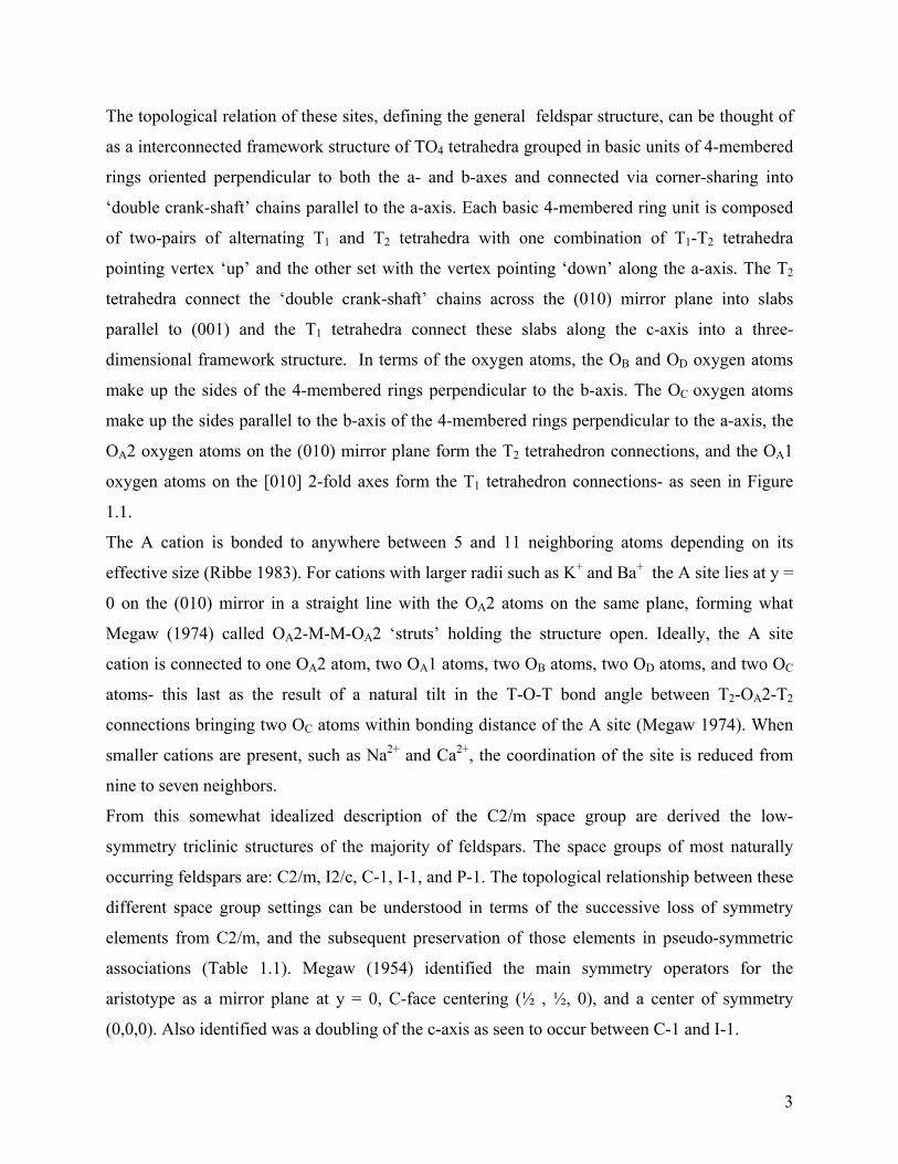
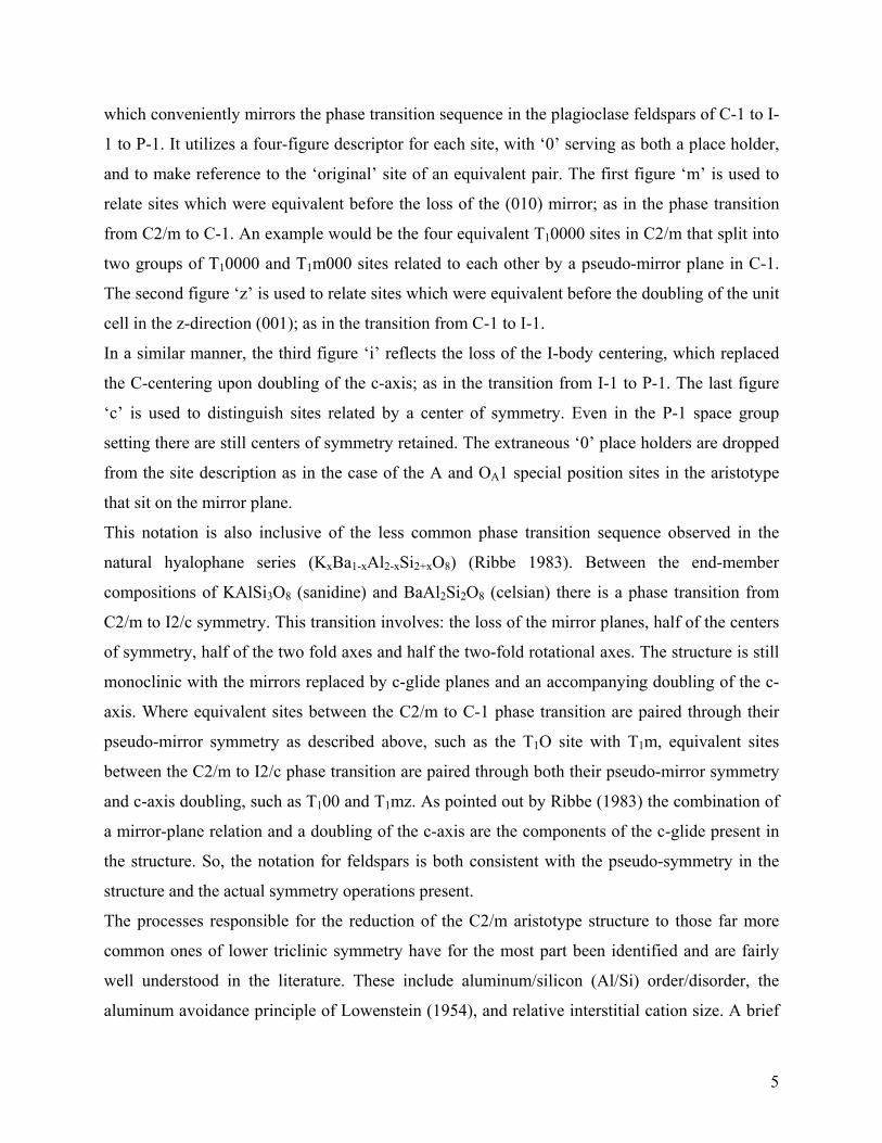
The topological relation of these sites, defining the general feldspar structure, can be thought of

as a interconnected framework structure of TO4 tetrahedra grouped in basic units of 4-membered

rings oriented perpendicular to both the a- and b-axes and connected via corner-sharing into

‘double crank-shaft’ chains parallel to the a-axis. Each basic 4-membered ring unit is composed

of two-pairs of alternating T1 and T2 tetrahedra with one combination of T1-T2 tetrahedra

pointing vertex ‘up’ and the other set with the vertex pointing ‘down’ along the a-axis. The T2

tetrahedra connect the ‘double crank-shaft’ chains across the (010) mirror plane into slabs

parallel to (001) and the T1 tetrahedra connect these slabs along the c-axis into a three-

dimensional framework structure. In terms of the oxygen atoms, the OB and OD oxygen atoms

what

egaw (1974) called OA2-M-M-OA2 ‘struts’ holding the structure open. Ideally, the A site

cation is connected to one OA2 atom, two OA1 atoms, two OB atoms, two OD atoms, and two OC

atoms- this last as the result of a natural tilt in the T-O-T bond angle between T2-OA2-T2

connections bringing two OC atoms within bonding distance of the A site (Megaw 1974). When

smaller cations are present, such as Na2+ and Ca2+, the coordination of the site is reduced from

nine to seven neighbors.

From this somewhat idealized description of the C2/m space group are derived the low-

symmetry triclinic structures of the majority of feldspars. The space groups of most naturally

occurring feldspars are: C2/m, I2/c, C-1, I-1, and P-1. The topological relationship between these

different space group settings can be understood in terms of the successive loss of symmetry

elements from C2/m, and the subsequent preservation of those elements in pseudo-symmetric

associations (Table 1.1). Megaw (1954) identified the main symmetry operators for the

aristotype as a mirror plane at y = 0, C-face centering (½ , ½, 0), and a center of symmetry

(0,0,0). Also identified was a doubling of the c-axis as seen to occur between C-1 and I-1.

make up the sides of the 4-membered rings perpendicular to the b-axis. The OC oxygen atoms

make up the sides parallel to the b-axis of the 4-membered rings perpendicular to the a-axis, the

OA2 oxygen atoms on the (010) mirror plane form the T2 tetrahedron connections, and the OA1

oxygen atoms on the [010] 2-fold axes form the T1 tetrahedron connections- as seen in Figure

1.1.

The A cation is bonded to anywhere between 5 and 11 neighboring atoms depending on its

effective size (Ribbe 1983). For cations with larger radii such as K+ and Ba+ the A site lies at y =

0 on the (010) mirror in a straight line with the OA2 atoms on the same plane, forming

M

3

C2/mSpace Group C-1 I2/c I-1 P-1

Pseudo-symmetry mirror c/2 (double z) mirror,c/2 (double z)

mirror,c/2 (double z), {a+b+c}/2 (i-centering), also z+i centering)

(c-

c lattice repeat 14 14 14 7 7 # formula units/cell 4 4 8 8 8

Multplicity 8 4 8 4 2 # Ind. Formula units 1/2 1 1 2 4

# ind. Atoms (tot) 8 13 13 26 52

# atoms (tot) 52 52 104 104 104

Bragg diffraction maxima

a (l = even or odd)

a (l = even or a,b; for h0l, l = even a,b

a(k+k = even,l = even), b (h+k = odd,l = odd), c (h+k = even,l = odd), d (h+k = odd,l = even) odd)

GEP sites B,

, D, , 2OB, 2OC, 4OB, 4OC, 4OD,

, 8OC, 8OD, 4OA1, 4OA2, 4M T1, T2, OOC, OD

2T1, 2T2, 2OB2OC, 2OOA1, OA2, M

2T1, 2T22OD, OA1, OA2, M

4T1, 4T2,2OA1, 2OA2, 2M 8T1, 8T2, 8OB

GEPs: T10000 T10000 T10000 T10000 T10000

T10000 T10000 T10000 T10000 T100i0

T10000 T10000 T10000 T10z00 T10z00

T10000 T10000 T10000 T10z00 T10zi0

T10000 T1m000 T10z00 T1m000 T1m000

T10000 T1m000 T10z00 T1m000 T1m0i0

T10000 T1m000 T10z00 T1mz00 T1mz00

T10000 T1m000 T10z00 T1mz00 T1mzi0

T1000c T1000c T1000c T1000c T1000c

T1000c T1000c T1000c T1000c T100ic

T1000c T1000c T1000c T10z0c T10z0c

T1000c T1000c T1000c T10z0c T10zic

T1000c T1m00c T10z0c T1m00c T1m00c

T1000c T1m00c T10z0c T1m00c T1m0ic

T1000c T1m00c T10z0c T1mz0c T1mz0c

T1000c T1m00c T10z0c T1mz0c T1mzic

SEP sites M, OA1,OA2 --- --- --- ---

SEPs: OA1000 OA1000 OA1000 OA1000 OA1000

OA1000 OA1000 OA1000 OA1000 OA10i0

OA1000 OA1000 OA1000 OA1z00 OA1z00

OA1000 OA1000 OA1000 OA1z00 OA1zi0

OA100c OA100c OA100c OA100c OA100c

OA100c OA100c OA100 OA100c OA10ic

OA100c OA100c OA100c OA1z0c OA1z0c OA100c OA100c OA100c OA1z0c OA1zic

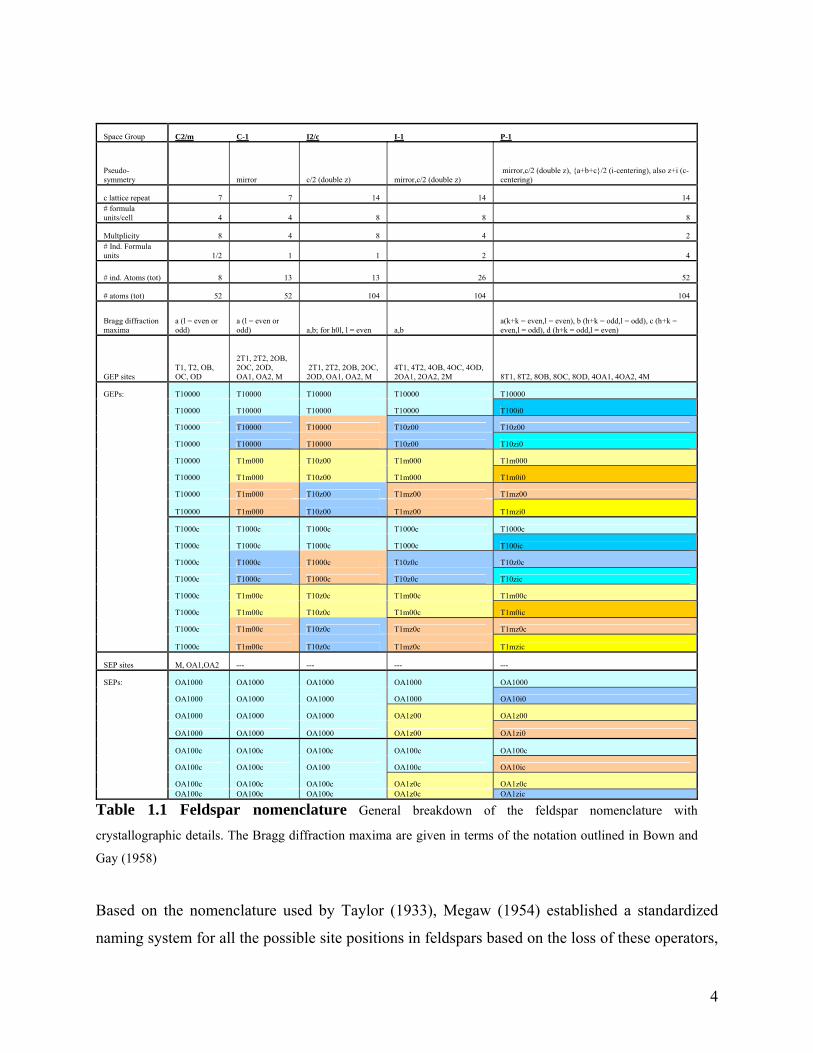
Table 1.1 Feldspar nomenclature General breakdown of the feldspar nomenclature with

crystallographic details. The Bragg diffraction maxima are given in terms of the notation outlined in Bown and

ay (1958) G

Based on the nomenclature used by Taylor (1933), Megaw (1954) established a standardized

naming system for all the possible site positions in feldspars based on the loss of these operators,

4

which conveniently mirrors the phase transition sequence in the plagioclase feldspars of C-1 to I-

1 to P-1. It utilizes a four-figure descriptor for each site, with ‘0’ serving as both a place holder,

and to make reference to the ‘original’ site of an equivalent pair. The first figure ‘m’ is used to

relate sites which were equivalent before the loss of the (010) mirror; as in the phase transition

from C2/m to C-1. An example would be the four equivalent T10000 sites in C2/m that split into

two groups of T10000 and T1m000 sites related to each other by a pseudo-mirror plane in C-1.

The second figure ‘z’ is used to relate sites which were equivalent before the doubling of the unit

in the case of the A and OA1 special position sites in the aristotype

nsistent with the pseudo-symmetry in the

aluminum avoidance principle of Lowenstein (1954), and relative interstitial cation size. A brief

cell in the z-direction (001); as in the transition from C-1 to I-1.

In a similar manner, the third figure ‘i’ reflects the loss of the I-body centering, which replaced

the C-centering upon doubling of the c-axis; as in the transition from I-1 to P-1. The last figure

‘c’ is used to distinguish sites related by a center of symmetry. Even in the P-1 space group

setting there are still centers of symmetry retained. The extraneous ‘0’ place holders are dropped

from the site description as

that sit on the mirror plane.

This notation is also inclusive of the less common phase transition sequence observed in the

natural hyalophane series (KxBa1-xAl2-xSi2+xO8) (Ribbe 1983). Between the end-member

compositions of KAlSi3O8 (sanidine) and BaAl2Si2O8 (celsian) there is a phase transition from

C2/m to I2/c symmetry. This transition involves: the loss of the mirror planes, half of the centers

of symmetry, half of the two fold axes and half the two-fold rotational axes. The structure is still

monoclinic with the mirrors replaced by c-glide planes and an accompanying doubling of the c-

axis. Where equivalent sites between the C2/m to C-1 phase transition are paired through their

pseudo-mirror symmetry as described above, such as the T1O site with T1m, equivalent sites

between the C2/m to I2/c phase transition are paired through both their pseudo-mirror symmetry

and c-axis doubling, such as T100 and T1mz. As pointed out by Ribbe (1983) the combination of

a mirror-plane relation and a doubling of the c-axis are the components of the c-glide present in

the structure. So, the notation for feldspars is both co

structure and the actual symmetry operations present.

The processes responsible for the reduction of the C2/m aristotype structure to those far more

common ones of lower triclinic symmetry have for the most part been identified and are fairly

well understood in the literature. These include aluminum/silicon (Al/Si) order/disorder, the

5

description of these processes is helpful in understanding how natural feldspars are classified and

vary in structure.

Aluminum and silicon fill the framework T sites of the feldspar structure and, upon cooling or

heating, can diffuse amongst the various site positions. For the aristotype sanidine composition,

it has been seen that Al prefers to occupy T1 sites over T2 sites, and when the mirror symmetry

element is lost it preferentially migrates to the T10 sites. Ribbe (1983) explained that the oxygen

atoms around the T1 site tend to be more closely bonded to the A cations than those around the

T2 sites, causing them to be slightly distorted and thus more favorable to Al on the grounds of

local electrostatic charge balancing. A convenient notation, first introduced by Kroll (1971),

describes the degree of ordering in the feldspar structure in terms of the average percentage of Al

occupancy per T site. These are represented by a lower case expression of their Megaw (1974)

label, based on a cumulative 0-1.0 scale. For the C2/m structure the general expression is 2t1 +

2t2 = 1.0, such that the total amount of Al in the structure is divided between the 2 T1 sites and

the 2T2 sites. Thus, for a completely disordered C2/m structure, t1 = t2 = 0.25, meaning that the

aluminum in the structure is on average divided evenly among the T1 and T2 sites, or there is a

random distribution of Al and Si among all the possible T sites, such that each has a quarter of

the total aluminum in the structure. This notation will be used later. Also complicating the slow

process of ordering of Al/Si is the apparent adherence in the feldspar topology to the ‘aluminum

avoidance principle’ which states that Al-O-Al bonds are electrostatically unfavorable in the

feldspar structure and avoided if at all possible during the process of ordering.

The combination of the ordering process with the ‘aluminum avoidance principle,’ leads to the

situation where symmetry must be broken as the segregation of Al and Si to particular locations

forces T-sites to non-equivalence. The C2/m structure with a ratio of 1:3::Al:Si can only

accommodate up to t1 = 0.5 or all the Al in the structure split evenly between the two T1 sites

with only Si on the two T2 sites. For ordering to continue the mirror plane between the two T1

sites must be broken in order for one to contain a higher percent occupancy of Al then the other,

as in the C2/m to C-1 phase transition (Ribbe 1983). Similarly, a fully ordered structure -where

an ideally perfect alternation pattern of Al and Si exists throughout the structure- with a ratio of

2:2::Si:Al, even requires a doubling along the c-axis as the neighboring ‘double crank-shaft’

slabs now have different arrangements of Al and Si. This process is responsible for the doubling

of the c-axis as seen in the phase transition from C-1 to I-1 and also from C2/m to I2/c.

6

The mineralogical nomenclature for feldspars is derived from its chemical, structural, and even

optical variations (Smith and Brown 1988). The general chemical variations seen in natural

samples have been outlined above as well as the general structural variants observed in terms of

their major governing processes. The optical variations will not be described herein (see Stewart

and Ribbe (1983) for a detailed explanation), but only mentioned in relation to specific

nomenclature based on them. The KAlSi3O8 (Or1.0Ab0An0) to NaAlSi3O8 (Or0Ab1.0An0) and the

NaAlSi3O8 (Or0Ab1.0An0) to CaAl2Si2O8 (Or0Ab0An1.0) compositional solid solution series in the

naturally occurring feldspar ternary will be described below.

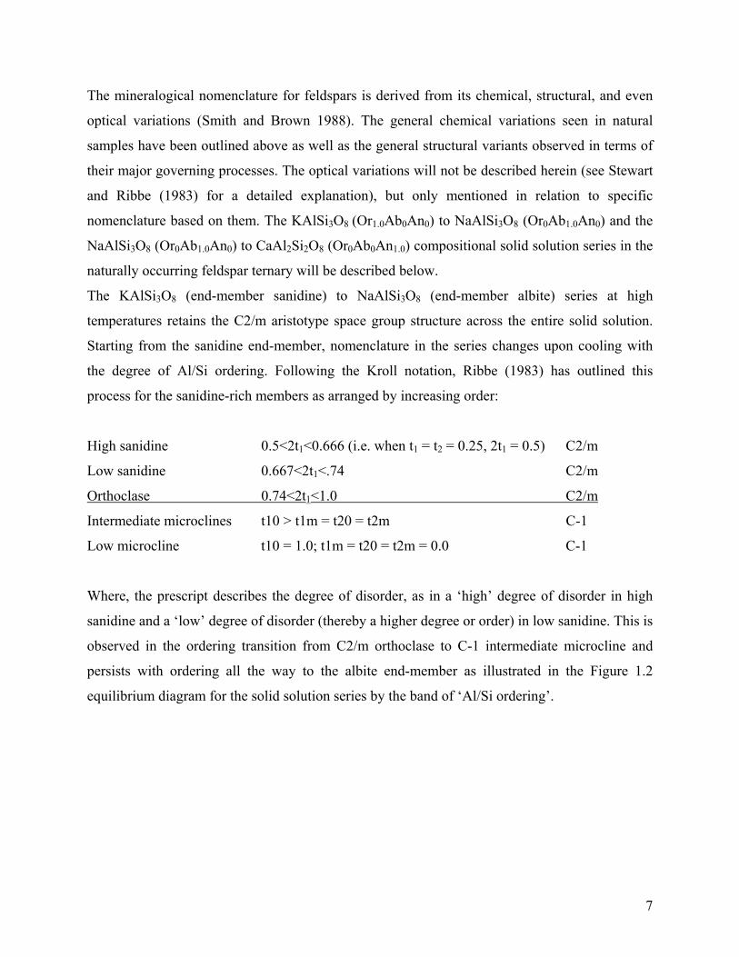
The KAlSi3O8 (end-member sanidine) to NaAlSi3O8 (end-member albite) series at high

temperatures retains the C2/m aristotype space group structure across the entire solid solution.

Starting from the sanidine end-member, nomenclature in the series changes upon cooling with

the degree of Al/Si ordering. Following the Kroll notation, Ribbe (1983) has outlined this

process for the sanidine-rich members as arranged by increasing order:

High sanidine 0.5<2t1<0.666 (i.e. when t1 = t2 = 0.25, 2t1 = 0.5) C2/m

Low sanidine 0.667<2t1<.74 C2/m

Orthoclase 0.74<2t1<1.0 C2/m

Intermediate microclines t10 > t1m = t20 = t2m C-1

Low microcline t10 = 1.0; t1m = t20 = t2m = 0.0 C-1

Where, the prescript describes the degree of disorder, as in a ‘high’ degree of disorder in high

sanidine and a ‘low’ degree of disorder (thereby a higher degree or order) in low sanidine. This is

observed in the ordering transition from C2/m orthoclase to C-1 intermediate microcline and

persists with ordering all the way to the albite end-member as illustrated in the Figure 1.2

equilibrium diagram for the solid solution series by the band of ‘Al/Si ordering’.

7

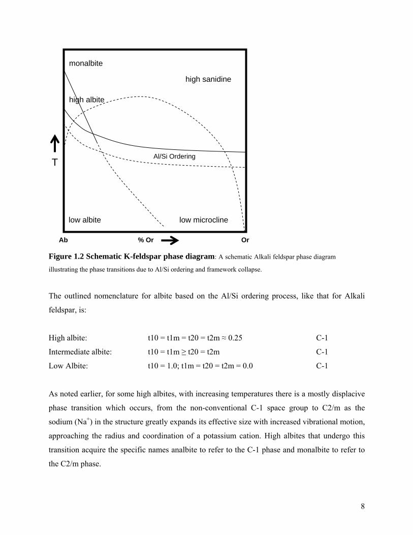
Figure 1.2 Schematic K-feldspar phase diagram: A schematic Alkali feldspar phase diagram

illustrating the phase transitions due to Al/Si ordering and framework collapse.

T

Ab Or% Or

Al/Si Ordering

high sanidine

low microcline low albite

high albite

monalbite

The outlined nomenclature for albite based on the Al/Si ordering process, like that for Alkali

feldspar, is:

High albite: t10 = t1m = t20 = t2m ≈ 0.25 C-1

Intermediate albite: t10 = t1m ≥ t20 = t2m C-1

Low Albite: t10 = 1.0; t1m = t20 = t2m = 0.0 C-1

As noted earlier, for some high albites, with increasing temperatures there is a mostly displacive

phase transition which occurs, from the non-conventional C-1 space group to C2/m as the

sodium (Na+) in the structure greatly expands its effective size with increased vibrational motion,

approaching the radius and coordination of a potassium cation. High albites that undergo this

transition acquire the specific names analbite to refer to the C-1 phase and monalbite to refer to

the C2/m phase.

8

Figure 1.3 Plagioclase phase diagram: Proposed sub-solidus equilibrium phase diagram from

Carpenter (1994) with structural transitions.

The NaAlSi3O8 (end-member albite) to CaAl2Si2O8 (end-member anorthite) solid solution has

ith increasing anorthite content a coupled substitution of Ca2+Al3+ for Na+Si4+ greatly

een the end-

tures, the

rdering process replacing the 1:3::Al:Si ratio of albite by the 2:2::Al:Si ratio of anorthite causes

been divided into different subgroups, originally based on petrographic optical differences

correlated to the mole percent of end-member anorthite in the chemical composition (see Figure

1.3 for specific divisions), and, as a whole, they are referred to as the ‘plagioclases’ or the

plagioclase solid solution series. The same high temperature analbite to monalbite transition

persists into the near end-member albite compositions of the plagioclase solid solution. For

increasing anorthite content, however, at least for a short range, the phase transition occurs at

higher and higher temperatures until the transition boundary intersects the liquidus, and melts

before the transition occurs (Carpenter 1994, and references therein). The equilibrium

temperature of this phase transition has also been seen to increase due to coupling between the

processes of the Na+ cation thermal expansion and a small component of Al/Si ordering

(Carpenter 1994).

W

complicates both the chemical and structural relationships of the plagioclases betw

member compositions (called intermediate plagioclases). As a result, at high tempera

o

9

an Al/Si ordering phase transition from C-1 to I-1. This relationship breaks down at lower

t10z0 = t1mzi = t1m00 = t1moi = t2000 = t200i = t2mz0 = t2mzi = 1.0; Al

s

s free energy of available for work or the ‘free energy’ as a

erivative of the Gibbs free energy

temperatures into an array of subsolidus relationships as proposed by Carpenter (1994) to include

a variety of equilibrium stability fields for e1 and e2 structures as seen in Figure 1.3. Figure 1.3

also shows the major phase transition in end-member anorthite at low temperatures from I-1 to

P-1. This is a displacive transition resulting from the further reduction of the coordination

number or ‘collapse’ of the structure around the Ca2+ cation site when the Al/Si is already full

ordered. The ordering in the P-1 structure is:

Anorthite: t1000 = t100i = t1mz0 = t1mzi = t20z0 = t20zi = t2m00 = t2moi = 0; Si

1.3 Thermodynamics

The Gibbs free energy characterizes the energy distribution accompanying chemical reaction ,

state transformations, and phase transitions. The Gibbs Free Energy equation of a single phase, G

= H +PV - TS, where G is the Gibb

function of the enthalpy (H), pressure (P), volume (V), temperature (T) and entropy (S). Based

on which order of the derivative of the Gibbs free energy equation is discontinuous at the phase

transition, it can be distinguished as either being first-order or second-order. Structurally, a

second-order phase transition involves changes that do not require bonds to be broken, such as

tilting, stretching, and rotation. These phase transitions have a discontinuity in the second

, βVPG

T

−=⎟⎟⎠

⎞⎜⎜⎝

⎛∂∂

2

2

op

d , where β is the compressibility. With

pressure, they show a change in the sl e. First

rder phase transitions have a discontinuity in the first-derivative of the Gibbs free

e of the trend for all parameters including volum

o

energy, VPG

T

=⎟⎠⎞

⎜⎝⎛∂∂ , They show a discontinuity or jump at the actual phase transition for

components such as volume with increasing pressure.

The thermodynamic behavior of minerals, especially in regards to phase transitions, seems to be

best described in terms of a specific solid-state adaptation of Gibbs free energy provided by

Landau Theory, which is based on a Taylor expansion in a macroscopic order parameter (Q). For

10

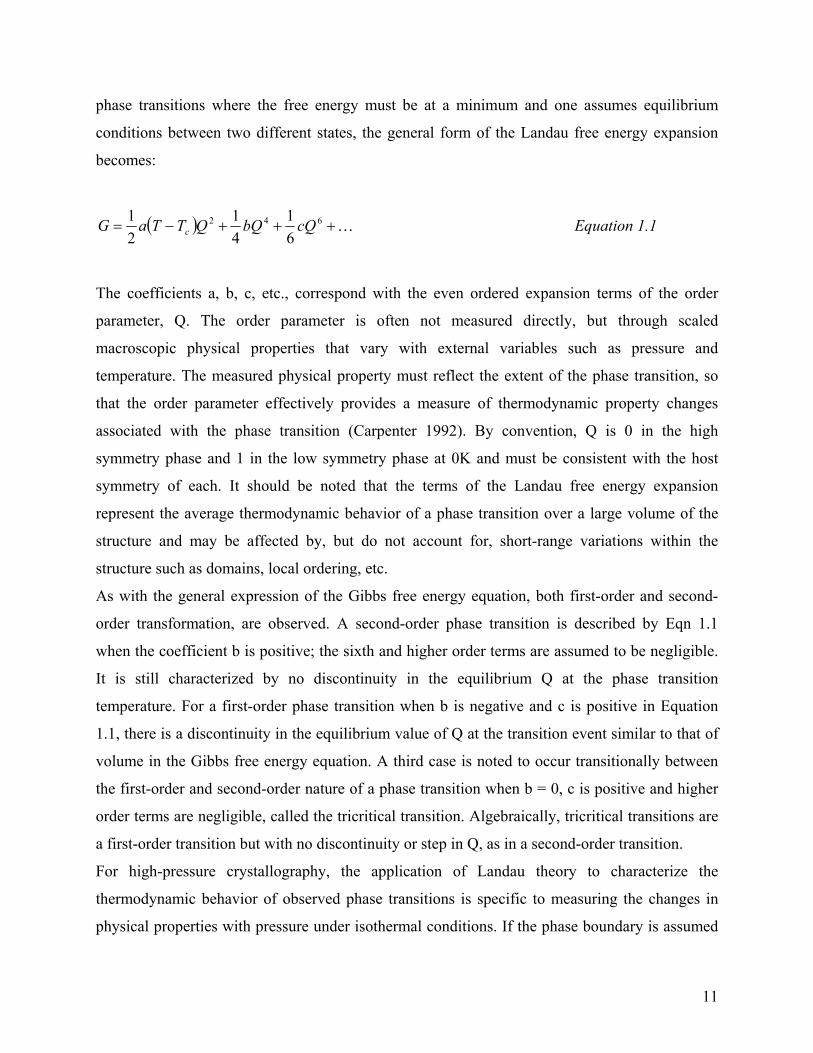
phase transitions where the free energy must be at a minimum and one assumes equilibrium

conditions between two different states, the general form of the Landau free energy expansion

becomes:

( ) K+++−= 642 111 cQbQQTTaG 642 c

The coefficients a, b, c, etc., correspond with the even ordered expansion terms of the order

parameter, Q. The order parameter is often not measured directly, but through scaled

macroscopic physical properties that vary with external variables such as pressure and

temperature. The measured physical property must reflect the extent of the phase transition, so

that the order parameter effectively provides a measure of thermodynamic property changes

associated with the phase transition (Carpenter 1992). By convention, Q is 0 in the high

symmetry phase and 1 in the low symmetry phase at 0K and must be consistent with the host

symmetry of each. It should be noted that the terms of the Landau free energy expans

Equation 1.1

ion

observed. A second-order phase transition is described by Eqn 1.1

w

gligible, called the tricritical transition. Algebraically, tricritical transitions are

first-order transition but with no discontinuity or step in Q, as in a second-order transition.

For high-pressure crystallography, the application of Landau theory to characterize the

thermodynamic behavior of observed phase transitions is specific to measuring the changes in

p hermal conditions. If the phase boundary is assumed

represent the average thermodynamic behavior of a phase transition over a large volume of the

structure and may be affected by, but do not account for, short-range variations within the

structure such as domains, local ordering, etc.

As with the general expression of the Gibbs free energy equation, both first-order and second-

order transformation, are

hen the coefficient b is positive; the sixth and higher order terms are assumed to be negligible.

It is still characterized by no discontinuity in the equilibrium Q at the phase transition

temperature. For a first-order phase transition when b is negative and c is positive in Equation

1.1, there is a discontinuity in the equilibrium value of Q at the transition event similar to that of

volume in the Gibbs free energy equation. A third case is noted to occur transitionally between

the first-order and second-order nature of a phase transition when b = 0, c is positive and higher

order terms are ne

a

hysical properties with pressure under isot

11

to be linear, the relationship between pressure and temperature for a constant experimental

temperature is given by:

( )expTTaaP c

vc −= where Tc is the transition temperature, Texp is the constant experimental

temperature, and Pc is the phase transition pressure (Carpenter 1992). Typically most processes

which are known to give rise to phase transitions in minerals all contribute to the overall

structural strain to some extent. The coupling between strain and the order parameter - assuming

the excess volume scales with Qo2 given a change in pressure like excess entropy given a change

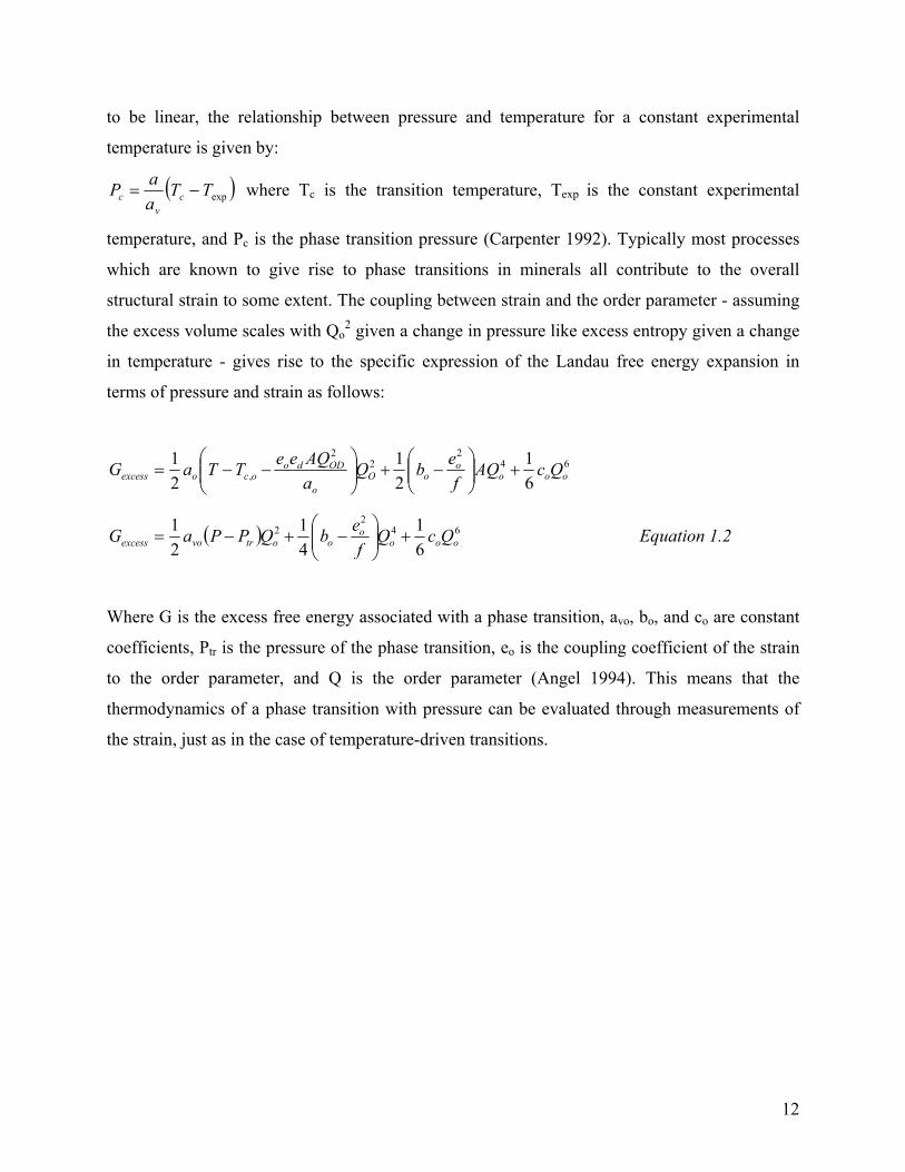
in temperature - gives rise to the specific expression of the Landau free energy expansion in

terms of pressure and strain as follows:

642

22

, 61

21

21

oooo

oOo

ODdoocoexcess QcAQ

febQ

aAQeeTTaG +⎟⎟

⎠

⎞⎜⎜⎝

⎛−+⎟⎟

⎠

⎞⎜⎜⎝

⎛−−=

( ) 642

2

61

41

21

oooo

ootrvoexcess QcQf

ebQPPaG +⎟⎟⎠

⎞⎜⎜⎝

⎛−+−= Equation 1.2

Where G is the excess free energy associated with a phase transition, avo, bo, and co are constant

coefficients, Ptr is the pressure of the phase transition, eo is the coupling coefficient of the strain

to the order parameter, and Q is the order parameter (Angel 1994). This means that the

thermodynamics of a phase transition with pressure can be evaluated through measurements of

the strain, just as in the case of temperature-driven transitions.

12

Chapter 2 Experimental Methods

2.1 Chapter Introduction This chapter will delineate the general laboratory methods used to investigate the plagioclase

feldspar behavior at high pressure, specifically single-crystal X-ray diffraction techniques and

the use of diamond anvil cells (DAC). Also, the general methods for solving crystal structures

and categorizing the elastic behavior of a medium (EoS and elasticity) will be laid out in detail.

2.2 X-ray diffraction

X-ray diffraction is the primary tool used for experimentally observing and determining the

crystal structure of most materials. Crystalline materials, by definition, have a certain periodicity

in their atomic arrangement (lattice) on the order of a few to a hundred or so Angstroms, within

two orders of magnitude of the wavelength of X-ray radiation (~1 Angstrom). This allows for the

electrons in an array to elastically scatter an incident X-ray beam and serve as a diffraction

grating, producing sharp maxima of constructive interference between the resulting propagated

electromagnetic (EM) waves.

The conditions for maximum constructive interference in any direction are given by the Laue

Equation:

a(cosα1 - cosα2) = nλ Equation 2.1

where a is the spacing of the lattice direction of interest, α1 is the angle of the incident beam

relative to the lattice direction, α2 is the angle of a propagated wave relative to the lattice

direction, n is the integer order of scattering, and λ is the wavelength of the incident radiation.

Three simultaneous Laue equations must be satisfied in Cartesian space for diffraction to occur.

A simplification of this description, derived from the Laue Equation, is the Bragg Equation:

13

nλ = 2dsinθ Equation 2.2

in which diffraction is described in terms of the reflection of the incident beam from a set of

lattice planes with spacing d and the angle 2θ, between the incident and diffracted beam.

Geometrically, the pattern of diffraction maxima, or peaks, is mapped by a reciprocal-space

lattice of inverse length and perpendicular directions to the real space lattice. So, a diffraction

peak can be seen as a vector in reciprocal space characterized by both its position, described by a

set of Miller Indices hkl, and its intensity (I). The measured intensity of a diffraction peak is a

function of the intensity of the incident beam, the square of amplitude of the structure factor, the

number of unit cells in the crystal, absorption and extinction in the crystal, the measuring

instrument detector distance, and other geometrical factors associated with the measurement

(Lorentz factor, etc.).

The structure factor is “the ratio of the amplitude scattered into the reflection by the contents of

the unit cell to the amplitude scattered into the same reflection by a free classical electron at the

origin”, assuming that all unit cells in the crystal are identical (time and space averaged). It

represents the total wave scattered by the unit cell contents.

The structure-factor equation is:

F(hkl) = ∑jƒj exp[2πi(hxj + kyj + lzj)exp[ -8π2u2jsin2(θ)/λ2]

= ∑jƒj(cos(2πiH·Xj) +isin(2πH·Xj)) Equation 2.3

Where ƒj is the atomic form factor, H is the reciprocal vector ha* + kb* + lc* corresponding the

reflection hkl, and X is the vector xa +yb + zc corresponding to the position of the atoms in the

unit cell. The atomic form factor scales directly with the number of electrons, but its amplitude is

dampened by the scattering angle (2θ), size of the atoms and wavelength (e.g. Miletich et al.

2005).

Complications arise from the I α |F(hkl)|2 relationship. First, because the intensity (I) scales with

the square of the structure factor, all measured diffraction patterns will have an imposed

inversion center (Friedel’s Law) whether the crystal has an inversion center or not. The only time

this symmetry is broken is if ‘anomalous scattering’ is present; it can be used to distinguish

enantiomers and absolute configuration. Secondly, the Fourier transform from the atom positions

14

to the structure factor requires information about the relative phase of each reflection that is lost

in the measured intensity values because of this squared relationship.

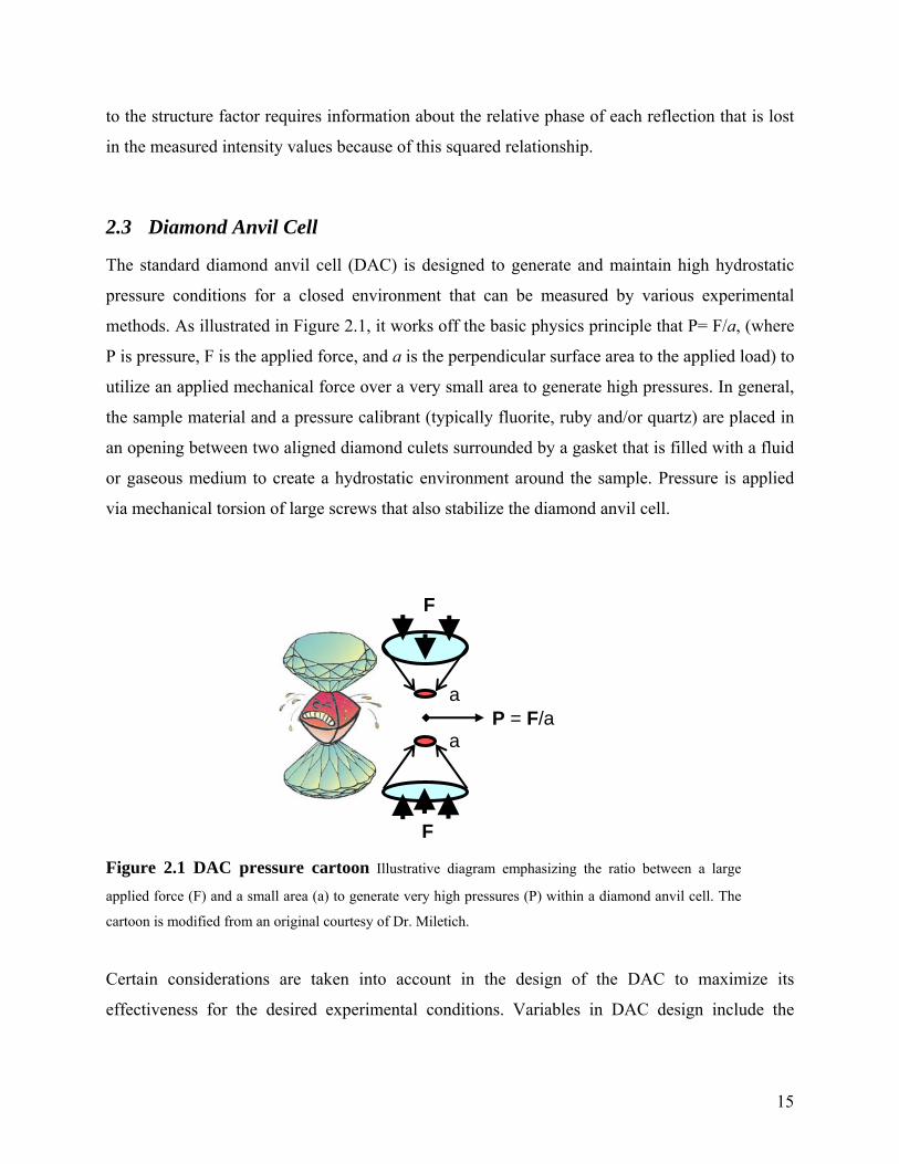
2.3 Diamond Anvil Cell

The standard diamond anvil cell (DAC) is designed to generate and maintain high hydrostatic

pressure conditions for a closed environment that can be measured by various experimental

methods. As illustrated in Figure 2.1, it works off the basic physics principle that P= F/a, (where

P is pressure, F is the applied force, and a is the perpendicular surface area to the applied load) to

utilize an applied mechanical force over a very small area to generate high pressures. In general,

the sample material and a pressure calibrant (typically fluorite, ruby and/or quartz) are placed in

an opening between two aligned diamond culets surrounded by a gasket that is filled with a fluid

or gaseous medium to create a hydrostatic environment around the sample. Pressure is applied

via mechanical torsion of large screws that also stabilize the diamond anvil cell.

Figure 2.1 DAC pressure cartoon Illustrative diagram emphasizing the ratio between a large

applied force (F) and a small area (a) to generate very high pressures (P) within a diamond anvil cell. The

cartoon is modified from an original courtesy of Dr. Miletich.

P = F/a

F

a

F

a

Certain considerations are taken into account in the design of the DAC to maximize its

effectiveness for the desired experimental conditions. Variables in DAC design include the

15

method of applied force, the stabilizing media, and transmitting media. Also, the sample

dimensions and reciprocal space coverage are important when choosing experimental details.

In terms of how the force is applied to the sample in order to generate high pressures, both the

types/dimensions of the diamonds and the method used to apply the mechanical load are

important. Diamond is ideal because it is highly transparent to a wide range of EM radiation

(5eV- 10keV) and it is the hardest known terrestrial material. It has excellent mechanical

conductivity and low thermal expansion, making it ideal to withstand large applied loads with

minimal mechanical deformation and minimizing its effect on background in EM experiments.

The dimensions of the diamond used for an experiment are factors of the sample volume, the

required pressure range, its effects on the background and absorption effects, and the overall

production costs. In general the thinner the diamonds, the lower the effect on the background and

absorption are, but the higher the chance of failure at lower pressures due to increased tensile

stresses within the anvils. Other materials sometimes utilized include sapphire and moissanite

(Miletich et al. 2005, Xu et al. 2002). Also, the greater the diamond anvil angle the greater its

load capacity. Various methods have been developed for applying the mechanical load to the

diamond anvils, including the use of lever arms, screws, and pneumatic drives. All are designed

to allow the alteration of the load in a gradual and continuous manner and attempt to limit the

obstruction of the actual measurement.

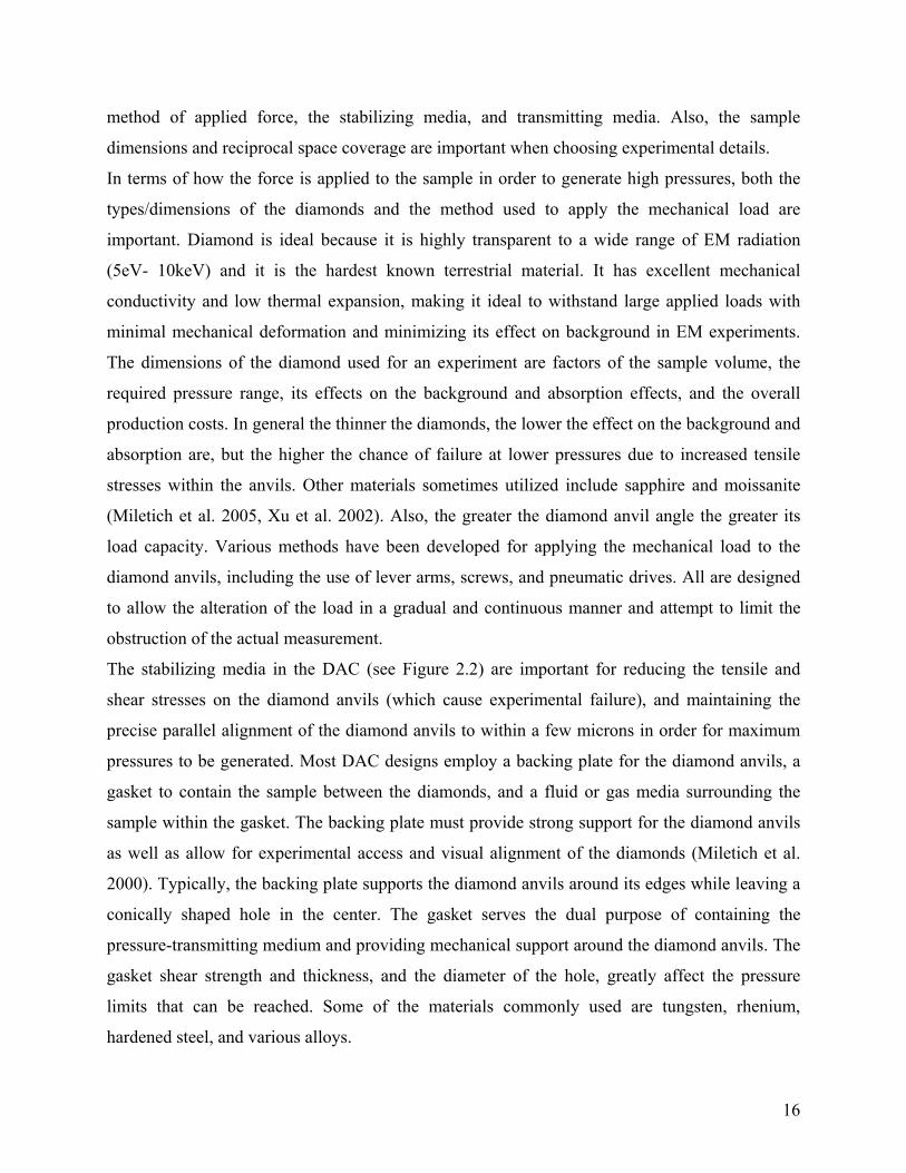
The stabilizing media in the DAC (see Figure 2.2) are important for reducing the tensile and

shear stresses on the diamond anvils (which cause experimental failure), and maintaining the

precise parallel alignment of the diamond anvils to within a few microns in order for maximum

pressures to be generated. Most DAC designs employ a backing plate for the diamond anvils, a

gasket to contain the sample between the diamonds, and a fluid or gas media surrounding the

sample within the gasket. The backing plate must provide strong support for the diamond anvils

as well as allow for experimental access and visual alignment of the diamonds (Miletich et al.

2000). Typically, the backing plate supports the diamond anvils around its edges while leaving a

conically shaped hole in the center. The gasket serves the dual purpose of containing the

pressure-transmitting medium and providing mechanical support around the diamond anvils. The

gasket shear strength and thickness, and the diameter of the hole, greatly affect the pressure

limits that can be reached. Some of the materials commonly used are tungsten, rhenium,

hardened steel, and various alloys.

16

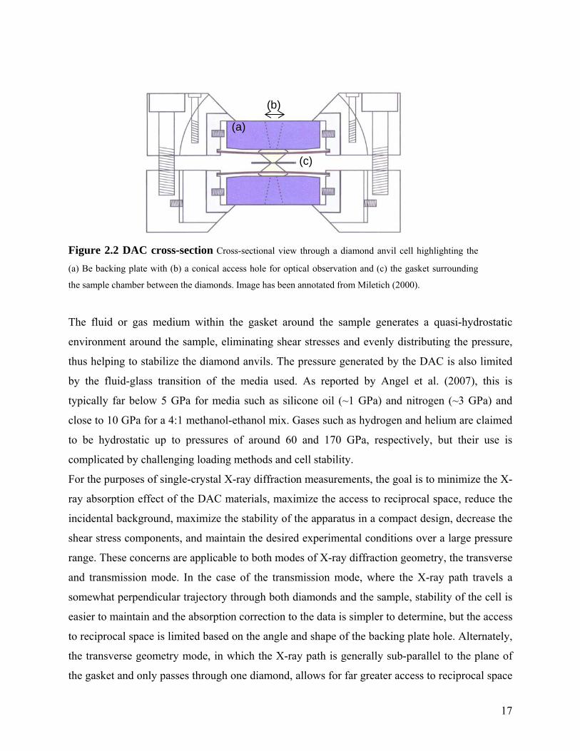
Figure 2.2 DAC cross-section Cross-sectional view through a diamond anvil cell highlighting the

(a) Be backing plate with (b) a conical access hole for optical observation and (c) the gasket surrounding

the sample chamber between the diamonds. Image has been annotated from Miletich (2000).

(a)

(b)

(c)

The fluid or gas medium within the gasket around the sample generates a quasi-hydrostatic

environment around the sample, eliminating shear stresses and evenly distributing the pressure,

thus helping to stabilize the diamond anvils. The pressure generated by the DAC is also limited

by the fluid-glass transition of the media used. As reported by Angel et al. (2007), this is

typically far below 5 GPa for media such as silicone oil (~1 GPa) and nitrogen (~3 GPa) and

close to 10 GPa for a 4:1 methanol-ethanol mix. Gases such as hydrogen and helium are claimed

to be hydrostatic up to pressures of around 60 and 170 GPa, respectively, but their use is

complicated by challenging loading methods and cell stability.

For the purposes of single-crystal X-ray diffraction measurements, the goal is to minimize the X-

ray absorption effect of the DAC materials, maximize the access to reciprocal space, reduce the

incidental background, maximize the stability of the apparatus in a compact design, decrease the

shear stress components, and maintain the desired experimental conditions over a large pressure

range. These concerns are applicable to both modes of X-ray diffraction geometry, the transverse

and transmission mode. In the case of the transmission mode, where the X-ray path travels a

somewhat perpendicular trajectory through both diamonds and the sample, stability of the cell is

easier to maintain and the absorption correction to the data is simpler to determine, but the access

to reciprocal space is limited based on the angle and shape of the backing plate hole. Alternately,

the transverse geometry mode, in which the X-ray path is generally sub-parallel to the plane of

the gasket and only passes through one diamond, allows for far greater access to reciprocal space

17

(up to ~85%), but has a very complicated absorption pathway which can alter as the gasket

deforms with pressure, and can have less overall stability in concession to the increased spatial

accessibility.

The series of experiments conducted for this thesis all used the transmission mode ETH-

he ETH-DAC has reduced dimensions 50 x 25 mm and 248g weight from its predecessors,

ell is applied through four M5 bolts paired with opposite threads at

diamond anvil cell, as modified (Miletich et al. 1999) from the “BGI” hybrid cell, which itself

incorporated design principles from both the original simpler Merrill-Bassett cell and Mao-Bell

cells. The ETH-DAC is specifically designed for diffraction experiments, but can be modified

based on the EM source of choice such as infrared, Raman, UV, etc. The particular cell used was

tailored for use in single-crystal X-ray diffraction experiments targeting a pressure range up to

ten Giga-Pascals (GPa).

(b) (a) (c) (e)(d) (f)

(g)

(h)

(i)

(j)

(k)(f) (l) (m) (n) (o)

(j) (j) (j) (j)

Figure 2.3 ETH-DAC schematic: Schematic decomposition of the transmission mode ETH-DAC

as modified from Miletich (2000). The labeled portions of the cell are as follows: (a) lower base platten

attached to goniometer, (b) guide pins, (c) XY transitional stage, (d) lower module base platten, (e) gasket

holder positioning pins, (f) Be plugs, (g) Be backing plates, (h) diamond anvils, (i) leaf springs, (j) M2 grub

screws, (k) rocking hemisphere, (l) upper base platen, (m) brass washers, (n) M5 bolts, and (o) M2

adjusting screws.

T

though it follows the original Merrill-Bassett design of having two square steel base plates

encasing opposing aligned diamond anvils. The reduced dimensions allow for easier use on

standard existing X-ray diffractometers originally used solely for single-crystal experiments in

air. The following specifications are taken from the ETH-DAC Users Manual by Miletich (2000)

and illustrated in Figure 2.3.

Mechanical pressure on the c

half the standard pitch, securing the two halves of the cell together and allowing for small

controlled alterations in the applied load by tightening the screws with Allen keys. The original

18

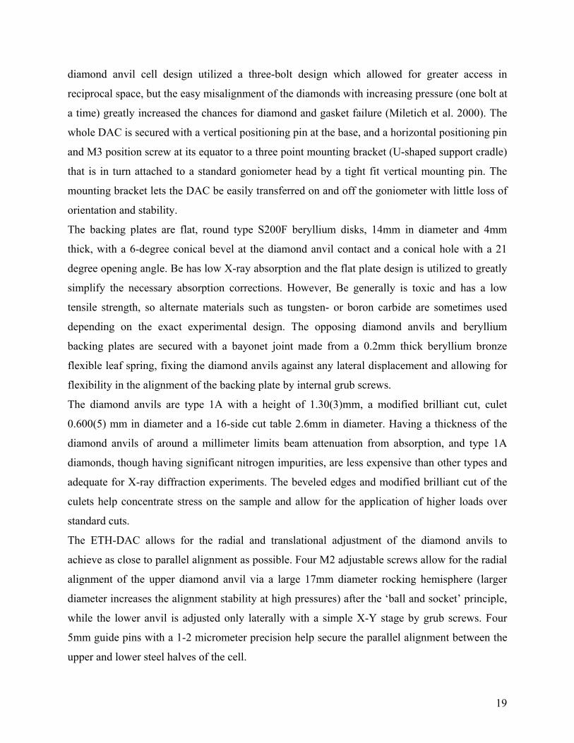
diamond anvil cell design utilized a three-bolt design which allowed for greater access in

reciprocal space, but the easy misalignment of the diamonds with increasing pressure (one bolt at

a time) greatly increased the chances for diamond and gasket failure (Miletich et al. 2000). The

whole DAC is secured with a vertical positioning pin at the base, and a horizontal positioning pin

and M3 position screw at its equator to a three point mounting bracket (U-shaped support cradle)

that is in turn attached to a standard goniometer head by a tight fit vertical mounting pin. The

mounting bracket lets the DAC be easily transferred on and off the goniometer with little loss of

orientation and stability.

The backing plates are flat, round type S200F beryllium disks, 14mm in diameter and 4mm

ified brilliant cut, culet

allows for the radial and translational adjustment of the diamond anvils to

upper and lower steel halves of the cell.

thick, with a 6-degree conical bevel at the diamond anvil contact and a conical hole with a 21

degree opening angle. Be has low X-ray absorption and the flat plate design is utilized to greatly

simplify the necessary absorption corrections. However, Be generally is toxic and has a low

tensile strength, so alternate materials such as tungsten- or boron carbide are sometimes used

depending on the exact experimental design. The opposing diamond anvils and beryllium

backing plates are secured with a bayonet joint made from a 0.2mm thick beryllium bronze

flexible leaf spring, fixing the diamond anvils against any lateral displacement and allowing for

flexibility in the alignment of the backing plate by internal grub screws.

The diamond anvils are type 1A with a height of 1.30(3)mm, a mod

0.600(5) mm in diameter and a 16-side cut table 2.6mm in diameter. Having a thickness of the

diamond anvils of around a millimeter limits beam attenuation from absorption, and type 1A

diamonds, though having significant nitrogen impurities, are less expensive than other types and

adequate for X-ray diffraction experiments. The beveled edges and modified brilliant cut of the

culets help concentrate stress on the sample and allow for the application of higher loads over

standard cuts.

The ETH-DAC

achieve as close to parallel alignment as possible. Four M2 adjustable screws allow for the radial

alignment of the upper diamond anvil via a large 17mm diameter rocking hemisphere (larger

diameter increases the alignment stability at high pressures) after the ‘ball and socket’ principle,

while the lower anvil is adjusted only laterally with a simple X-Y stage by grub screws. Four

5mm guide pins with a 1-2 micrometer precision help secure the parallel alignment between the

19

Between the diamond anvils, a T301 hardened stainless-steel gasket (~ 1cm x 1cm x 250

microns) is fixed with tack to a 22mm diameter brass-plate gasket holder attached to the lower

ssure calibrant is typically a

ce peak shift in the Raman spectra as detailed by

the pressure condition of the experiment

steel base plate by 3 positioning pins, to allow for easy removal and replacement of the gasket.

The T301 gasket is pre-indented between the diamond anvils to a thickness between 90 and 120

microns. A sample chamber is drilled by spark-corrosion in the center of the indentation to a

diameter between 260 and 300 microns and filled with a 4:1 methanol-ethanol pressure fluid.

These specifications are chosen with an average single crystal sample size of 100 x 100 x 30

microns in mind and a goal of around 10 GPa maximum pressure.

In high-pressure X-ray diffraction experiments, the sample chamber in the DAC contains an

internal pressure standard in addition to the sample itself. The pre

single crystal of a known substance that is relatively small in physical size and possesses some

measurable property which changes in a consistent and known way with pressure. It must also be

a high-symmetry material that has a small unit-cell volume, is stable in air and the pressure

medium used, and generally produces strong, sharp diffraction peaks (Hazen and Finger 1981).

Traditionally both ruby and fluorite have been used, while more recently quartz has been the

internal pressure standard of choice for its smaller uncertainty in pressure determination over

both ruby and fluorite.

Ruby was initially used for its space saving size (a few microns diameter) in the gasket and the

accuracy of measurement via ruby fluorescen

Forman et al. (1972). However a strong temperature dependence of the ruby spectrum, the

necessity of physically conducting the measurement away from that of the sample measurement,

and error propagation through peak fitting procedures all lead to an overall pressure uncertainty

higher than that of either fluorite or quartz standards. It is still widely used despite its drawbacks

as a quick method for calibrating pressure changes applied to a DAC or in cases where neither

quartz nor fluorite crystals will fit in the gasket hole.

Fluorite was used throughout the 1980s and 1990s as a popular internal pressure standard. Unlike

ruby, its unit cell parameters are used to calibrate

through an experimentally determined Equation of State (EoS). The EoS for fluorite was first

documented by Hazen and Finger (1981) and refined by Angel et al (1993). It has the advantage

over ruby of being measured under the same environmental conditions as the sample and

generates an improved precision in the pressure uncertainties to just over ~0.03 GPa. However,

20

large uncertainties in the determination of K’, peak broadening after around 7 GPa and a phase

transition at 9.2 GPa make pressure determinations at higher pressures impossible (Angel et al.

1997).

Quartz was presented as a pressure standard by Angel et al. (1997) who determined its EoS

based on fluorite measurements and independent ultrasonic measurements of the elastic

e analysis

To describe the crystal structure of a material, the lattice parameters, crystal symmetry, and

ll be known or, at least, they must be experimentally approachable.

α radiation source, monochromator,

constants (McSkimmin et al. 1965). Quartz, unlike fluorite, is stable to over 10 GPa and has a

smaller bulk modulus. When the unit-cell volume is determined to a precision of 1 part in 10,000

or better, the resulting uncertainty in pressure is less than 0.01 GPa. The hexagonal symmetry of

quartz also has the added advantage of allowing elastic calculations to be made to check for non-

hydrostatic stresses.

2.4 Structur

unique atom positions must a

As noted above, the position of diffracted X-ray peaks can be used to determine the lattice

parameters of a structure while the peak intensities contain extractable information about the

crystal symmetry and unique atom positions. Structure analysis begins with the collection of raw

data, which is then indexed, integrated, solved and refined.

For this thesis, high-pressure DAC intensity data collections were carried out primarily with

Oxford Diffraction Xcalibur diffractometers using a MoK

kappa-geometry cradle, and point detector. MoKα radiation is used for DAC experiments over

the alternatives of either Cu or Ag sources because of the low total transmission through the

DAC (~0.2%) of Cu radiation, and a degradation of intensity data due to the shorter wavelength

of Ag radiation (Angel et al. 2000). The use of a monochromator reduces the background

(improving the precision of the calculated intensities). Utilizing a kappa-geometry cradle over

the traditional Eulerian geometry, allows for greater freedom of movement for chi values under

90 degrees and for the generation of higher diffracted intensities due to its smaller overall size

(i.e. shorter detector distance, less absorption from air scatter). A point detector was used rather

than a CCD detector because the point detector can be collimated to reduce background

21

intensities, and to avoid issues of structured background and area-imaging resolution issues

inherent with CCD detectors (Angel et al. 2000).

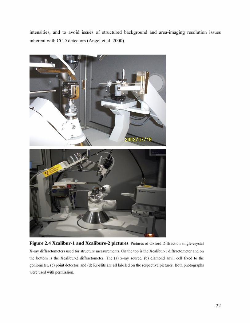
Figure 2.4 Xcalibur-1 and Xcalibure-2 pictures: Pictures of Oxford Di

(a (b

(c

(a

(b(d (c

ffraction single-crystal

X-ray diffractometers used for structure measurements. On the top is the Xcalibur-1 diffractometer and on

the bottom is the Xcalibur-2 diffractometer. The (a) x-ray source, (b) diamond anvil cell fixed to the

goniometer, (c) point detector, and (d) Re-slits are all labeled on the respective pictures. Both photographs

were used with permission.

22

Specifically an Oxford Diffraction Xcalibur-1 and an Oxford Diffraction Xcalibur-2

diffractometer, as shown in Figure 2.4, were used. Both diffractometers were operated at 50kV,

40 mA with either a 0.5mm or 0.8mm collimator and at a detector distance of ~130mm. For

experiments conducted on the Xcalibur-1, detector slits of 0.5 x 2.0 mm were used as well as an

extra Re-slit designed in-house by Dr. Jing Zhou to further reduce background intensities. The

Xcalibur-2 was not equipped with Re-slits, and detector slits of either the same as those on

Xcalibur-1 or slightly larger (1.0 x 2.0 mm) were used, depending on availability at the time of

the experiment. In all cases Be plugs were placed in the conical holes of the Be backing plates of

the DACs to simplify the absorption correction.

Prior to measurement of a sample in a DAC, or air, it must be aligned accurately with the center

of the X-ray beam on the instrument. This is typically done visually, using either an optical

microscope or an orientated camera mount to view the crystal close up. The general procedure is

to rotate the crystal or DAC in space 180 degrees around each of its three principal axes (phi-

coordinate system) and minimize the displacement along each until the point of reference is

static on the axis of rotation. On Xcalibur diffractometers the offsets from the diffractometer

center are further corrected using the offsets calculated with the WinIntergrStp integration

software (Angel 2003) from a small data set of the position of 20 to 50 strong long angle

reflections.

The first step in solving the structure of a sample is to define the position of the diffracted peaks

by ‘indexing’ each reflection with a set of Miller Indices based on the calculated unit cell

parameters. For this to be done the exact orientation of reciprocal lattice vectors with respect to a

common ortho-normal basis set must be known, as is given by the UB matrix. Given the known

positions of the goniometer, detector and diffracted beams on the detector, the UB matrix defines

the following relationship (Busing and Levy 1967):

(x,y,z)phi-axis = UB . h Equation 2.4

where the position of the reciprocal lattice vectors (h), are transformed from the reciprocal lattice

basis to an orthonormal basis relative to the crystal by the B matrix , and rotationally transformed

from the orthonormal basis relative to the crystal to one on the ‘phi-axis coordinate’ system of

the instrument goniometer by the U matrix. The phi-axis coordinate system definition differs

23

between different machines depending on the definition of the basis vectors and the circle

parities, so the orientation matrix for a given crystal changes in its U component.

In high-pressure DAC experiments the UB matrix is initially determined from the two-reflection

orientation method, as detailed by Busing and Levy (1967), from the known setting angles of

two reflections, with assigned indices, and the crystal unit-cell parameters. The unit-cell

parameters are either known from previously published material on the same sample or from

indexing of the crystal of interest in air with CCD data using the Duisenberg mixed method

(Clegg et al. 2004). Complications arise from the mis-indexing of the reflections used, improper

centering of the DAC, and ambiguity in the constructed vector-triples sign (Angel et al. 2000).

These make the degree of error between the calculated and observed angles as well as the

calculation of a third non-co-planar reflection, extremely important parameters in deriving the

correct UB matrix.

Intensity data collections on the Xcalibur diffractometers all utilized omega scans in a ‘fixed phi-

mode’ setting of around 1500 reflections from 2 to 40 degrees in theta. Fixed phi mode is

designed to maximize the number of observable reflections by as much as 40% over the

bisecting mode by fixing the phi angle to zero (Finger and King 1978).

Once peak measurements have been collected, integration of the data is an important step in

extracting the actual intensities from the reflection profiles and correcting for instrumental

factors and background. For DAC experiments conducted here, the WinIntegrStp v3.5

integration program of Angel (2003) was used to integrate the measured data by peak-fitting of

individual reflections with pseudo-Voigt functions after Pavese and Artioli (1996). The program

also contained algorithms for refining the background, FWHM, peak position and intensity,

mixing parameter, I-ratio, etc, to improve the fit of each peak and to maximize the quality of the

integrated intensities. An absorption correction must be made to intensities extracted from DAC

data, due to absorption by the crystal and various components of the DAC apparatus. The

absorption corrections were made with the Absorb v6.0 program by Angel (2004a) modified

from Burnham (1966). Lastly, the intensity data were merged, based on crystal symmetry

constraints, and processed with criteria for outlier rejection with the Average v2.2 program of

Angel (2004b). The final output of the integration process is a list of corrected integrated

intensities, or F2 values, for each symmetry-averaged set of measured hkl reflections.

24

The last step in structure analysis is to combine the structure model information (unit cell

parameters, space group, symmetry constraints, assumed atom positions, etc), hkl positions, and

corresponding F2 values. The structure model information for DAC experiments is typically

already determined from a structure solved from a CCD data set collected in air, or previously

published structures. The refinement process follows a least-squares procedure of minimizing the

“residual” or differences between a structure factor equation calculated from the model structure

parameters and the structure factor of the actual processed data, F(obs) – F(calc). In general the

‘fit’ of the model is evaluated statistically using the criteria of ‘weighted-chi-squared’, the

goodness of fit, ‘weighted R-value’ and ‘un-weighted R-value’.

Unfortunately, diffractometers such as the Xcalibur-1 and -2 are designed for accurate intensity

measurements and cannot be used to get the unit-cell parameter precision of 1 part in 30,000

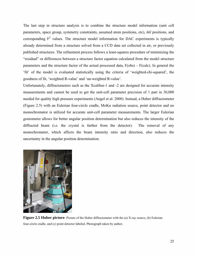
needed for quality high pressure experiments (Angel et al. 2000). Instead, a Huber diffractometer

(Figure 2.5) with an Eulerian four-circle cradle, MoKα radiation source, point detector and no

monochromator is utilized for accurate unit-cell parameter measurements. The larger Eulerian

goniometer allows for better angular position determination but also reduces the intensity of the

diffracted beam (i.e. the crystal is farther from the detector). The removal of any

monochromator, which affects the beam intensity ratio and direction, also reduces the

uncertainty in the angular position determination.

Figure 2.5 Huber picture: Picture of the Huber diffractometer with the (a) X-ray source, (b) Eulerian

four-circle cradle, and (c) point detector labeled. Photograph taken by author.

(a

(b

(c

25

The UB matrix on the Huber diffractometer is determined via the two-reflection orientation

method as on the Xcalibur-1 and Xcalibur-2 diffractometers. However, crystal offsets and cell

parameters are determined from data of strong reflections collected using the 8-position

centering method, modified from Hamilton (1974) by King and Finger (1979), under the

SINGLE software documented in Angel et al (2000). Crystal offsets are determined from the 8-

position centering of one reflection, and corrected, before 10-20 strong reflections are centered

with the same method and used to directly calculate the unit-cell parameters with a ‘vector least-

squares’ fit of the diffraction vectors detailed by Ralph and Finger (1982). The advantage of 8-

position centering is that it reduces the effect of the effective diffraction center, uneven

background, DAC absorption and shadowing, etc., all of which can vary from reflection to

reflection, thus reducing the uncertainty in the cell parameter calculations.

Precise unit-cell parameters, in addition to factoring in to the determination of a materials

structure, can be used to evaluate the relationship in high-pressure experiments between the

applied pressure and the deformation of the material. The measure of both of these, the applied

pressure and resultant deformation, are tensors or physical quantities whose components

transform according to specific laws.

2.5 Elasticity

The applied stress to a body is characterized by the stress tensor, ijσ , which is both homogeneous

and symmetric, and defines the relation:

jiji lp σ= Equation 2.5

Where is a force transmitted across a surface area perpendicular to the unit vector . ip jl

Likewise, the deformation of a body resulting from an applied stress is characterized by the

strain tensor, ijε , which, given that the distortion is homogenous and that the tensor is symmetric,

defines the relation between the displacement of a point due to strain, , and the position vector

of the point, , as:

iu

jx

26

jiji xu ε= Equation 2.6

Both are second-rank field tensors with 9 components in a 3x3 matrix where the components

along the diagonal (σii or εii) represent normal stresses or tensile strains and the other off-

diagonal components (σij or εij) represent shear stresses or strains. The symmetric nature of the

strain tensor, like the stress tensor, makes jiij εε = (or jiij σσ = for stress), reducing it to only six

independent components.

Because stress and strain are both symmetric second-rank tensors, they can be described by their

three principal axes, the diagonal normal components, or “three mutually perpendicular

directions in a body which remain perpendicular during deformation” (Nye 1957). This is

possible because the transformation of a quadric surface, as defined by its principal axes, follows

the rules of transformation of a tensor. So the stress tensor is represented by three orthogonal

uniaxial stress components along the directions of the principal axes. For triclinic materials

where there are no symmetry constraints over those intrinsic to the second-rank tensor, the

orientation of the principle axes is completely arbitrary and must be defined in addition to the

magnitude of the three principal components to specify the tensor.

The relationship between homogeneous stress and strain is given by the generalized Hooke’s

Law:

klijklij s σε = Equation 2.7

where represents the fourth-rank elastic compliance tensor relating nine equations with nine

terms each, giving it a total of 81 components. However,

ijkls

ijσ and ijε are symmetric so,

reducing 81 components to only 36 components. Also, in the linear elastic

regime where Hooke’s law applies and under isothermal conditions, the free energy is dependent

only on the state of the body. This makes the tensor symmetric and thereby further reduces

the 36 components to 21 independent ones. Symmetry constraints imposed in crystal systems

above triclinic reduce the number of independent components even more, down to only three in

the cubic system.

jiklijklijlkijkl ssss == ,

ijkls

27

Tensor suffix notation can be simplified by converting it down to matrix notation after the Voigt

convention. Matrix notation reduces consecutive pairs of tensor suffixes, always starting from

the end of the suffix chain, to a single number from one to six in their place. The convention is to

replace doublet ones (11) with a single one (1), doublet twos (22) with a single two (2), doublet

threes (33) with a single three (3), two-three combinations (23,32) with a four (4), three-one

combinations (31,13) with a five (5), and one-two combinations (12,21) with a six (6). So, the

tensor suffix variables which by definition vary between one and three vary between one and six

in matrix notation.

This simplification necessitates the addition into some tensor definitions of additional

multiplication factors for the final expression in matrix notation to be as compact as possible.

Thus for the strain tensor when ji ≠ (the off-diagonal terms) a factor of ½ is introduced in front

of each respective term in the corresponding matrix. Similarly, in the compliance tensor, a factor

of 2 is introduced when either term in the matrix notation is a 4,5,or 6 and a factor of 4 is

introduced when both terms in matrix notation are 4,5,or 6. So in the conversion from tensor

notion to matrix notation of the elasticity relationship between stress and strain, the

multiplication factors cancel out to give a concise final expression of:

jijiklijklij ss σεσε =→= Equation 2.8

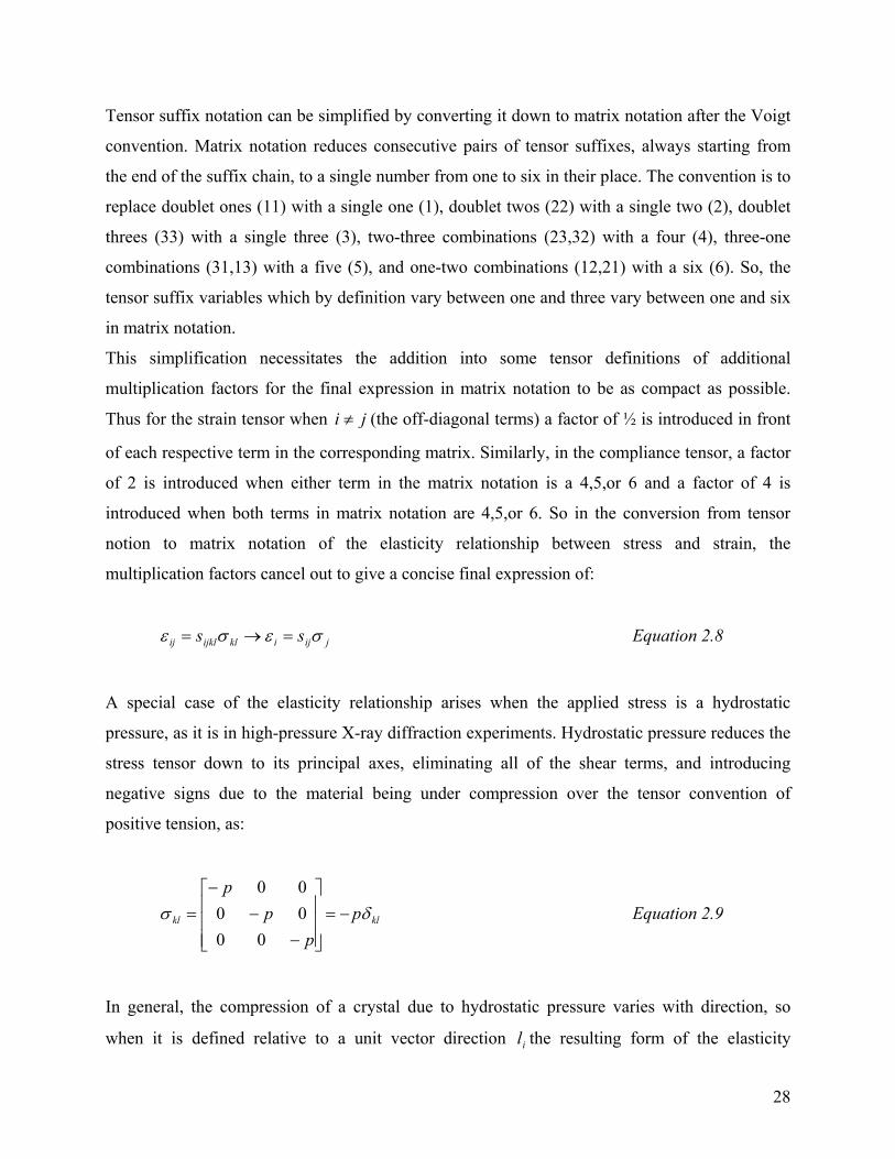
A special case of the elasticity relationship arises when the applied stress is a hydrostatic

pressure, as it is in high-pressure X-ray diffraction experiments. Hydrostatic pressure reduces the

stress tensor down to its principal axes, eliminating all of the shear terms, and introducing

negative signs due to the material being under compression over the tensor convention of

positive tension, as:

Equation 2.9 klkl pp

pp

δσ −=⎥⎥⎥

⎦

⎤

⎢⎢⎢

⎣

⎡

−−

−=

000000

In general, the compression of a crystal due to hydrostatic pressure varies with direction, so

when it is defined relative to a unit vector direction the resulting form of the elasticity il

28

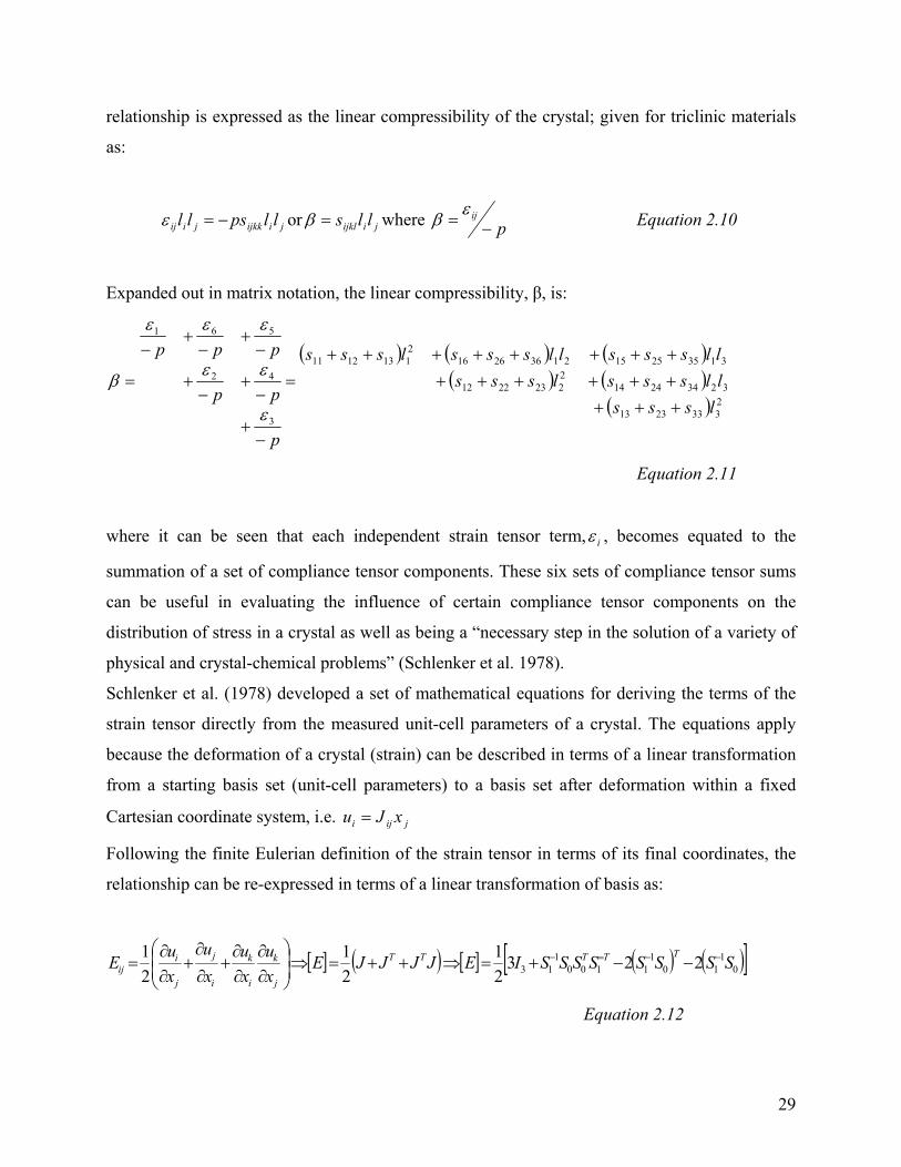
relationship is expressed as the linear compressibility of the crystal; given for triclinic materials

as:

jiijkkjiij llpsll −=ε or jiijkl lls=β where pij−=

εβ Equation 2.10

Expanded out in matrix notation, the linear compressibility, β, is:

( ) ( ) (( ) (

( ) 23332313

3234241422232212

313525152136261621131211

3

42

561

lsssllssslsssllsssllssslsss

p

pp

ppp

+++++++++++++++++

=

−+

−+

−+

−+

−+

−

=

ε

εε))

εεε

β

Equation 2.11

where it can be seen that each independent strain tensor term, iε , becomes equated to the

summation of a set of compliance tensor components. These six sets of compliance tensor sums

can be useful in evaluating the influence of certain compliance tensor components on the

distribution of stress in a crystal as well as being a “necessary step in the solution of a variety of

physical and crystal-chemical problems” (Schlenker et al. 1978).

Schlenker et al. (1978) developed a set of mathematical equations for deriving the terms of the

strain tensor directly from the measured unit-cell parameters of a crystal. The equations apply

because the deformation of a crystal (strain) can be described in terms of a linear transformation

from a starting basis set (unit-cell parameters) to a basis set after deformation within a fixed

Cartesian coordinate system, i.e. jiji xJu =

Following the finite Eulerian definition of the strain tensor in terms of its final coordinates, the

relationship can be re-expressed in terms of a linear transformation of basis as:

[ ] ( ) [ ] ( ) ( )[ ]01

101

11001

13 22321

21

21 SSSSSSSSIEJJJJE

xu

xu

xu

xuE TTTTT

j

k

i

k

i

j

j

iij

−−=− −−+=⇒++=⇒⎟⎟⎠

⎞⎜⎜⎝

⎛

∂∂

∂∂

+∂

∂+

∂∂

=

Equation 2.12

29

The terms in the final expression of the equation represent the calculation steps required to

convert from the coordinate system of the crystal to a fixed Cartesian system via a set of

matrixes defined by Schlenker et al. (1978). As noted above, for the expression of the strain

tensor in the triclinic system, the orientation of an orthogonal basis set is arbitrary so must be

pre-defined.

The expression developed is not calculating the exact, but the incremental strain tensor

components, as the calculated values are from two sets of unit cell parameters measured before

and after a crystal has experienced deformation over an interval of applied pressure. The

assumption is that the pressure interval P∆ is sufficiently small to equate the derived linearized

incremental strain components to the actual sums of the compliance tensor components through

linear compressibility (Brown et al. 2006).

From the feldspar unit-cell parameters measured for this thesis, compliance tensor sums were

calculated using the WinStrain program developed by Dr. Ohashi and modified by Dr. Angel

(VT). The orientation for the Cartesian axis system followed that of Brown et al. (2006) where

the y-axis was aligned parallel to the b-axis of the crystal, the x-axis was set along the a*

direction and the z-axis orthogonal to the first two axes following a right-handed coordinate

convention. This is ideal for evaluating the strain in feldspars where the softest direction is

typically along the a* direction, and the b-axis is the longest in magnitude. Each strain tensor

term was calculated, plotted versus the mid-point of each incremental pressure interval, and

extrapolated back to get an estimated value of each compliance tensor sum at zero pressure, P=0.

As with linear compressibility, where the relationship between stress and strain is characterized

by its variation with direction, the volume compressibility of a crystal further averages the

effects of compression to be equal in all directions thereby giving the exact relationship between

volume and pressure. When stress is an applied hydrostatic pressure, and thus there are no off-

diagonal shear terms, the generalized Hooke’s law can be simplified to:

( psiikkii −==∆ )ε or iikkii spp =−=∆− ε Equation 2.13

where ∆ represents the isotropic change in volume of a unit-cube. In matrix notation this

expression becomes:

30

332313

232212

131211

333333223311

223322222211

113311221111

ssssss

sss

sssssssss

siikk

++++++

++=

++++++++

=

Equation 2.14

The volume compressibility is typically defined as its reciprocal value called the Bulk Modulus,

K; that isiikksK 1= . The volume compressibility of a crystal is commonly approximated by an

Equation of State which fits the calculated variations in unit-cell volume upon compression of a

crystal with increasing pressure.

2.6 Equation of State

An Equation of State (EoS) is in general a relation between two properties such as volume (V)

and temperature (T), and specifically in high-pressure X-ray diffraction experiments, it is the

relation between volume and pressure (P). This relationship, although not based on definitive

thermodynamic principles, can be formulated in a number of ways depending on the physical

assumptions made. Such Equations of State include the Murnaghan, Natural Strain, Birch-

Murnaghan (B-M) and Vinet Equations of State (Angel 2000). All these Equations of State are

parameterized fits to P-V data, almost always in terms of the Bulk Modulus, K, and its pressure

derivatives, K’ and K’’-- all assumed to be isothermal for the high-pressure experiments

reported herein. Their exact definitions are as follows:

VPVK

∂∂

−= PKK∂∂

=′ 2

2

PKK

∂∂

=′′ Equation 2.15

The Murnaghan EoS (Murnaghan 1937) is the simplest, based on the assumption that K varies

linearly with pressure, and is widely used to calculate metamorphic phase equilibria. Slightly

more complex is the Natural Strain EoS developed by Poirier and Tarantola (1998). It is based

on the “Hencky” definition of linear strain. Similarly, the Birch-Murnaghan EoS (Birch 1947)

assumes that the compressional strain energy of a solid is expressible as a Taylor series

31

expansion of the finite Eulerian strain, fE. Vinet et al. (1987) also developed an EoS tailored for

solids under very high compression that do not express significant degrees of internal structural

freedom, based on general inter-atomic potentials.

The Birch-Murnaghan EoS is the one routinely applied to high-pressure X-ray diffraction

experiments of natural Earth solids in many geophysical applications, and is the specific one

utilized for this thesis. The Murnaghan EoS has been found to be applicable only up to

compressions of 10% after which it deviates strongly from either the Birch-Murnaghan or Vinet

EoS that produce values for the bulk modulus closest to those of independent determinations

(Angel et al. 1997). The Natural Strain EoS also deviates from these last two and is only

improved in fits with additional parameters so its use may not be as elegant or exact. The Vinet

and Birch-Murnaghan EoS do not differ significantly for compressions up to 0.85 and for values

of K’ between 3.3 and 7. Outside of this range the Vinet EoS yields the higher overall values in P

or V with compression. However, the Vinet EoS contains extra assumptions over those of the

Birch-Murnaghan EoS which leads to slightly fewer circumstances where it is applicable,

making the B-M EoS the best for general use.

The Birch-Murnaghan EoS, as expanded to a 4th order in the free energy is defined as follows:

( ) ( ) ( )( ) ⎟⎠

⎞⎜⎝

⎛⎟⎠⎞

⎜⎝⎛ +−′−′+′′+−′++= 2

02

50 9

3534234

231213 EEEE fKKKKfKffKP

Equation 2.16

The finite Eulerian strain in this equation is given as:

2

13

2

0

⎥⎥⎦

⎤

⎢⎢⎣

⎡−⎟

⎠⎞

⎜⎝⎛

=VV

f E Equation 2.17

The fourth-order expression fits all the parameters of V0, K, K’, and K’’, which represent

physical properties of the material. The Birch-Murnaghan EoS can also be truncated to the

second or third order in the energy depending on the fit to the data, as each has successively

independent terms. The third-order truncation fixes the coefficient of fE2 to zero, so there are only

three parameters of V0, K, and K’ in the equation, with the value of K’’ determined by these

32

three parameters (Anderson 1995). The second-order truncation sets the coefficient of fE to zero,

so only V0 and K are refineable parameters, with K’ fixed to 4 and the higher-order terms such as

K’’ ignored.

The EoS is fit in the form P = f(V) to measured data via the least squares process using the

EoSFit5.2 program (Angel 2003) and truncated to the appropriate order based on evaluation of

statistical measures to assess the ‘fit’ such as weighted-chi-squared, goodness of fit and variance-

covariance. Specifically the process of least squares attempts to minimize the weighted-chi

squared value of:

((2

,,,2 ,1 ∑ −

−=

n

iiobsiobsiobsiw TVEoSPw

mnχ )) Equation 2.18

where m is the number of parameters refined and n is the number of data points, each with a

weight w defined through the effective variance method by:

( )22

222

2

11

KVK

w

TVP

i

ασσσσ

+⎟⎠⎞

⎜⎝⎛+

== Equation 2.19

In general this method leads to the V0 and K0 parameters displaying the largest influence on the

data fit, and thus should always be the first values refined before other terms are added to the

EoS (Angel 2000).

The visual evaluation of the Birch-Murnaghan EoS is done by rewriting the expression in terms

of a normalized stress, F, versus a finite strain, fE, where

( )[ ] 25

213 EE ffPF+

= and the EoS, after Stacey et al. (1981) is:

( ) ( )( ) ...93534

234

23 2

00

00

0 +⎟⎠⎞

⎜⎝⎛ +−′−′+′′+−′+= EEE fKKKKKfKKKF Equation 2.20

33

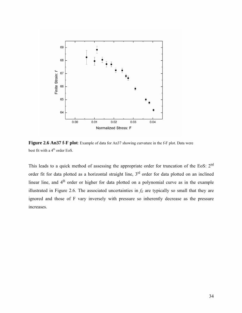
Figure 2.6 An37 f-F plot: Example of data for An37 showing curvature in the f-F plot. Data were

best fit with a 4th order EoS.

This leads to a quick method of assessing the appropriate order for truncation of the EoS: 2nd

order fit for data plotted as a horizontal straight line, 3rd order for data plotted on an inclined

linear line, and 4th order or higher for data plotted on a polynomial curve as in the example

illustrated in Figure 2.6. The associated uncertainties in fE are typically so small that they are

ignored and those of F vary inversely with pressure so inherently decrease as the pressure

increases.

34

Chapter 3 Results 3.1 Chapter Introduction This chapter will build on the background information provided in the previous chapters and

report the experimental results of the studies of plagioclase feldspars at high pressures.

3.2 Unit-cell parameters

The results detailed below are from a combination of previously collected and published data as

well as from data collected specifically for this thesis. All sample data were collected in high-

pressure DAC diffractometer experiments using a 4:1 methanol-ethanol fluid pressure medium,

but with several different pressure standards including ruby, fluorite, and quartz. Table 3.1

outlines some of the physical sample details including general composition, when it has been

determined, sample petrogenesis, and papers in which either previous sample descriptions or

results have been published. Samples will be labeled only after their percent anorthite

composition for simplicity. The An00 sample was previously measured by Benusa et al. (2005).

Likewise, data from samples An20, An36, An45, An68, An77, and An89 were previously

collected by Dr. Angel from 1993 to 1997. The samples measured during the process of this

thesis include An37, An50, An60, and An96.

35

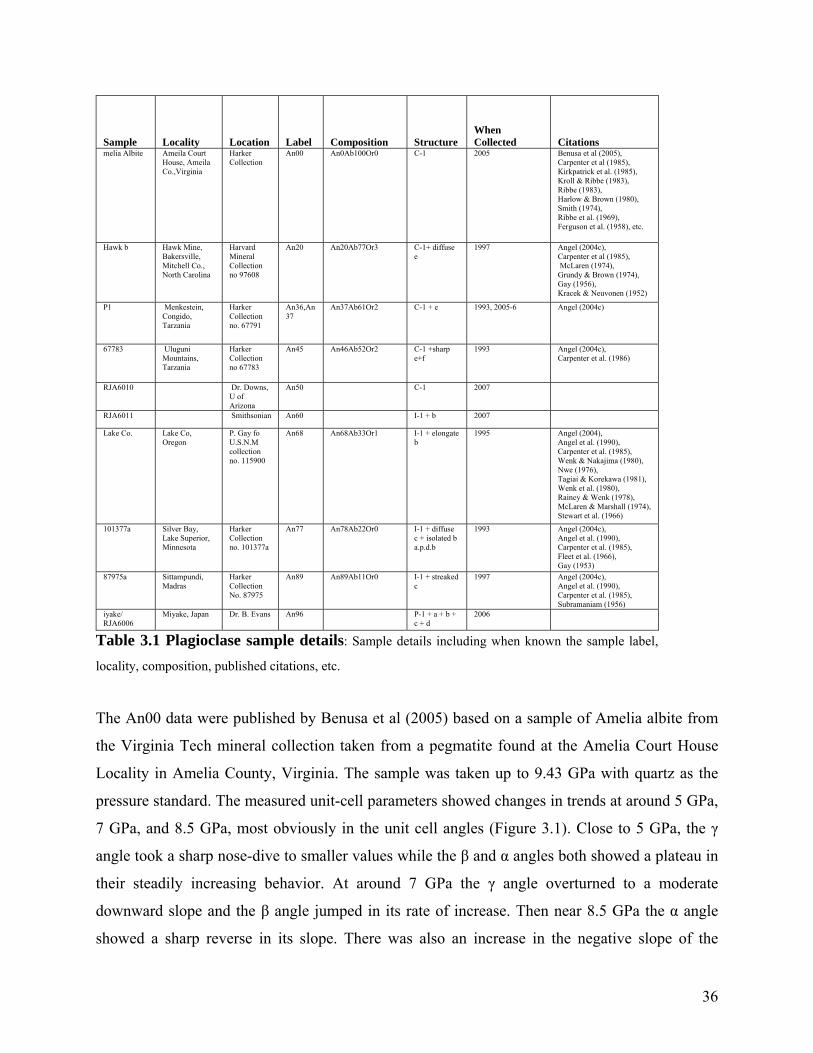
Sample Locality Location Label Composition Structure When Collected Citations

melia Albite Ameila Court House, Ameila Co.,Virginia

Harker Collection

An00 An0Ab100Or0 C-1 2005 Benusa et al (2005), Carpenter et al (1985), Kirkpatrick et al. (1985), Kroll & Ribbe (1983), Ribbe (1983), Harlow & Brown (1980), Smith (1974), Ribbe et al. (1969), Ferguson et al. (1958), etc.

Hawk b Hawk Mine, Bakersville, Mitchell Co., North Carolina

Harvard Mineral Collection no 97608

An20 An20Ab77Or3 C-1+ diffuse e

1997 Angel (2004c), Carpenter et al (1985), McLaren (1974), Grundy & Brown (1974), Gay (1956), Kracek & Neuvonen (1952)

P1 Menkestein, Congido, Tarzania

Harker Collection no. 67791

An36,An37

An37Ab61Or2 C-1 + e 1993, 2005-6 Angel (2004c)

67783 Uluguni Mountains, Tarzania

Harker Collection no 67783

An45 An46Ab52Or2 C-1 +sharp e+f

1993 Angel (2004c), Carpenter et al. (1986)

RJA6010 Dr. Downs, U of Arizona

An50 C-1 2007

RJA6011 Smithsonian An60 I-1 + b 2007

Lake Co. Lake Co, Oregon

P. Gay fo U.S.N.M collection no. 115900

An68 An68Ab33Or1 I-1 + elongate b

1995 Angel (2004), Angel et al. (1990), Carpenter et al. (1985), Wenk & Nakajima (1980), Nwe (1976), Tagiai & Korekawa (1981), Wenk et al. (1980), Rainey & Wenk (1978), McLaren & Marshall (1974), Stewart et al. (1966)

101377a Silver Bay, Lake Superior, Minnesota

Harker Collection no. 101377a

An77 An78Ab22Or0 I-1 + diffuse c + isolated b a.p.d.b

1993 Angel (2004c), Angel et al. (1990), Carpenter et al. (1985), Fleet et al. (1966), Gay (1953)

87975a Sittampundi, Madras

Harker Collection No. 87975

An89 An89Ab11Or0 I-1 + streaked c

1997 Angel (2004c), Angel et al. (1990), Carpenter et al. (1985), Subramaniam (1956)

iyake/ RJA6006

Miyake, Japan Dr. B. Evans An96 P-1 + a + b + c + d

2006

Table 3.1 Plagioclase sample details: Sample details including when known the sample label,

locality, composition, published citations, etc.

The An00 data were published by Benusa et al (2005) based on a sample of Amelia albite from

the Virginia Tech mineral collection taken from a pegmatite found at the Amelia Court House

Locality in Amelia County, Virginia. The sample was taken up to 9.43 GPa with quartz as the

pressure standard. The measured unit-cell parameters showed changes in trends at around 5 GPa,

7 GPa, and 8.5 GPa, most obviously in the unit cell angles (Figure 3.1). Close to 5 GPa, the γ

angle took a sharp nose-dive to smaller values while the β and α angles both showed a plateau in

their steadily increasing behavior. At around 7 GPa the γ angle overturned to a moderate

downward slope and the β angle jumped in its rate of increase. Then near 8.5 GPa the α angle

showed a sharp reverse in its slope. There was also an increase in the negative slope of the

36

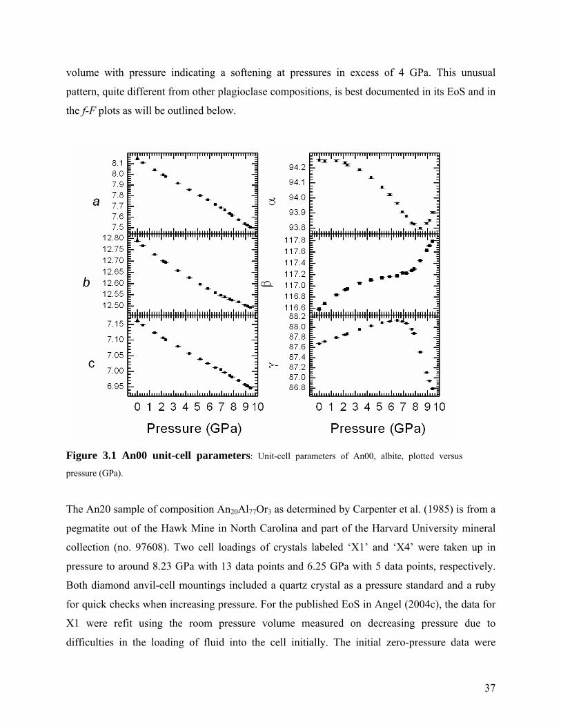
volume with pressure indicating a softening at pressures in excess of 4 GPa. This unusual

pattern, quite different from other plagioclase compositions, is best documented in its EoS and in

the f-F plots as will be outlined below.

Figure 3.1 An00 unit-cell parameters: Unit-cell parameters of An00, albite, plotted versus

pressure (GPa).

The An20 sample of composition An20Al77Or3 as determined by Carpenter et al. (1985) is from a

pegmatite out of the Hawk Mine in North Carolina and part of the Harvard University mineral

collection (no. 97608). Two cell loadings of crystals labeled ‘X1’ and ‘X4’ were taken up in

pressure to around 8.23 GPa with 13 data points and 6.25 GPa with 5 data points, respectively.

Both diamond anvil-cell mountings included a quartz crystal as a pressure standard and a ruby

for quick checks when increasing pressure. For the published EoS in Angel (2004c), the data for

X1 were refit using the room pressure volume measured on decreasing pressure due to

difficulties in the loading of fluid into the cell initially. The initial zero-pressure data were

37

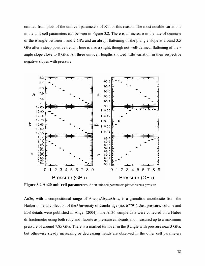
omitted from plots of the unit-cell parameters of X1 for this reason. The most notable variations

in the unit-cell parameters can be seen in Figure 3.2. There is an increase in the rate of decrease

of the α angle between 1 and 2 GPa and an abrupt flattening of the β angle slope at around 3.5

GPa after a steep positive trend. There is also a slight, though not well-defined, flattening of the γ

angle slope close to 8 GPa. All three unit-cell lengths showed little variation in their respective

negative slopes with pressure.

Figure 3.2 An20 unit-cell parameters: An20 unit-cell parameters plotted versus pressure.

An36, with a compositional range of An35-38Ab60-62Or2-3, is a granulitic anorthosite from the

Harker mineral collection of the University of Cambridge (no. 67791). Just pressure, volume and

EoS details were published in Angel (2004). The An36 sample data were collected on a Huber

diffractometer using both ruby and fluorite as pressure calibrants and measured up to a maximum

pressure of around 7.85 GPa. There is a marked turnover in the β angle with pressure near 3 GPa,

but otherwise steady increasing or decreasing trends are observed in the other cell parameters

38

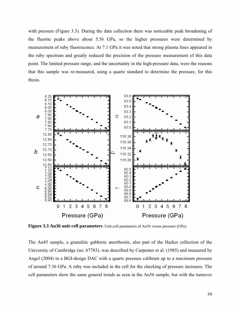
with pressure (Figure 3.3). During the data collection there was noticeable peak broadening of

the fluorite peaks above about 5.56 GPa, so the higher pressures were determined by

measurement of ruby fluorescence. At 7.1 GPa it was noted that strong plasma lines appeared in

the ruby spectrum and greatly reduced the precision of the pressure measurement of this data

point. The limited pressure range, and the uncertainty in the high-pressure data, were the reasons

that this sample was re-measured, using a quartz standard to determine the pressure, for this

thesis.

Figure 3.3 An36 unit-cell parameters: Unit-cell parameters of An36 versus pressure (GPa).

The An45 sample, a granulitic gabbroic anorthosite, also part of the Harker collection of the

University of Cambridge (no. 67783), was described by Carpenter et al. (1985) and measured by

Angel (2004) in a BGI-design DAC with a quartz pressure calibrant up to a maximum pressure

of around 7.36 GPa. A ruby was included in the cell for the checking of pressure increases. The

cell parameters show the same general trends as seen in the An36 sample, but with the turnover

39

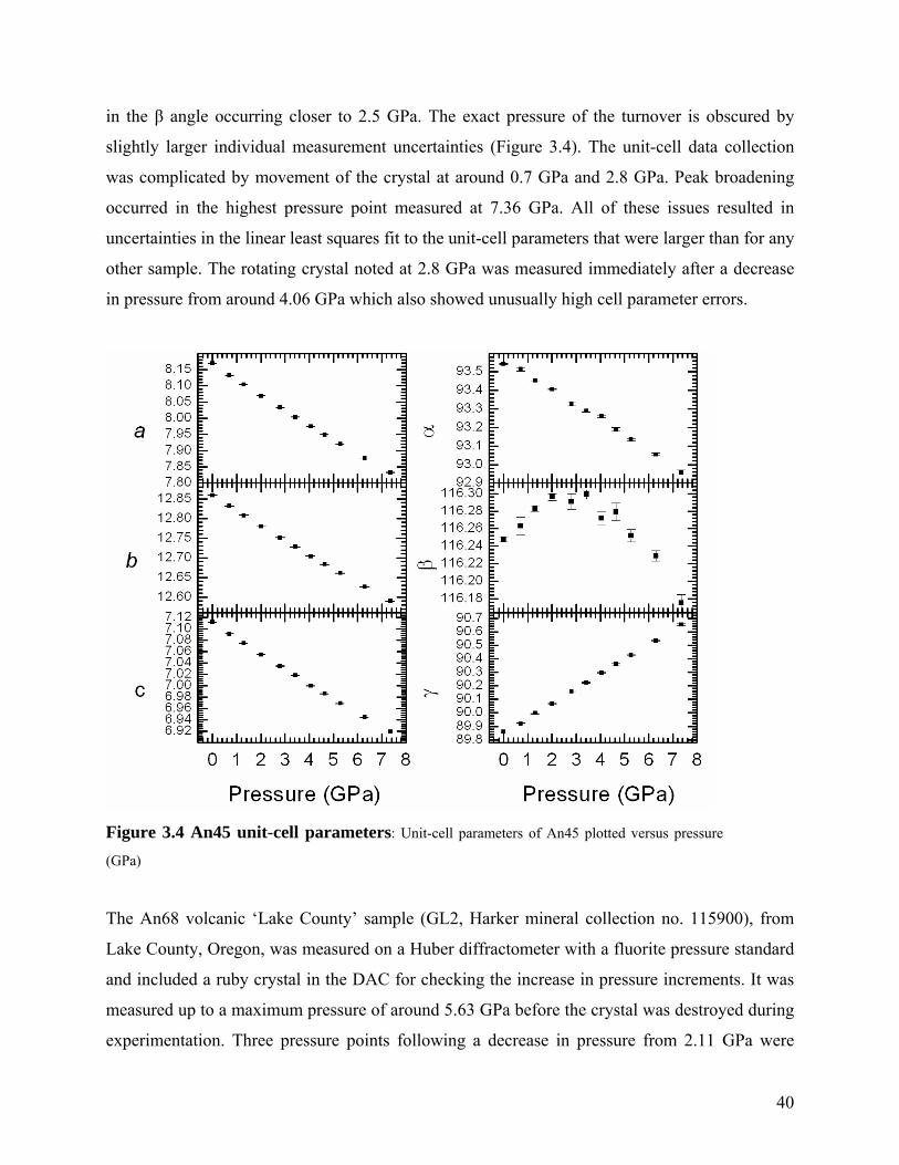
in the β angle occurring closer to 2.5 GPa. The exact pressure of the turnover is obscured by

slightly larger individual measurement uncertainties (Figure 3.4). The unit-cell data collection

was complicated by movement of the crystal at around 0.7 GPa and 2.8 GPa. Peak broadening

occurred in the highest pressure point measured at 7.36 GPa. All of these issues resulted in

uncertainties in the linear least squares fit to the unit-cell parameters that were larger than for any

other sample. The rotating crystal noted at 2.8 GPa was measured immediately after a decrease

in pressure from around 4.06 GPa which also showed unusually high cell parameter errors.

Figure 3.4 An45 unit-cell parameters: Unit-cell parameters of An45 plotted versus pressure

(GPa)

The An68 volcanic ‘Lake County’ sample (GL2, Harker mineral collection no. 115900), from

Lake County, Oregon, was measured on a Huber diffractometer with a fluorite pressure standard

and included a ruby crystal in the DAC for checking the increase in pressure increments. It was

measured up to a maximum pressure of around 5.63 GPa before the crystal was destroyed during

experimentation. Three pressure points following a decrease in pressure from 2.11 GPa were

40

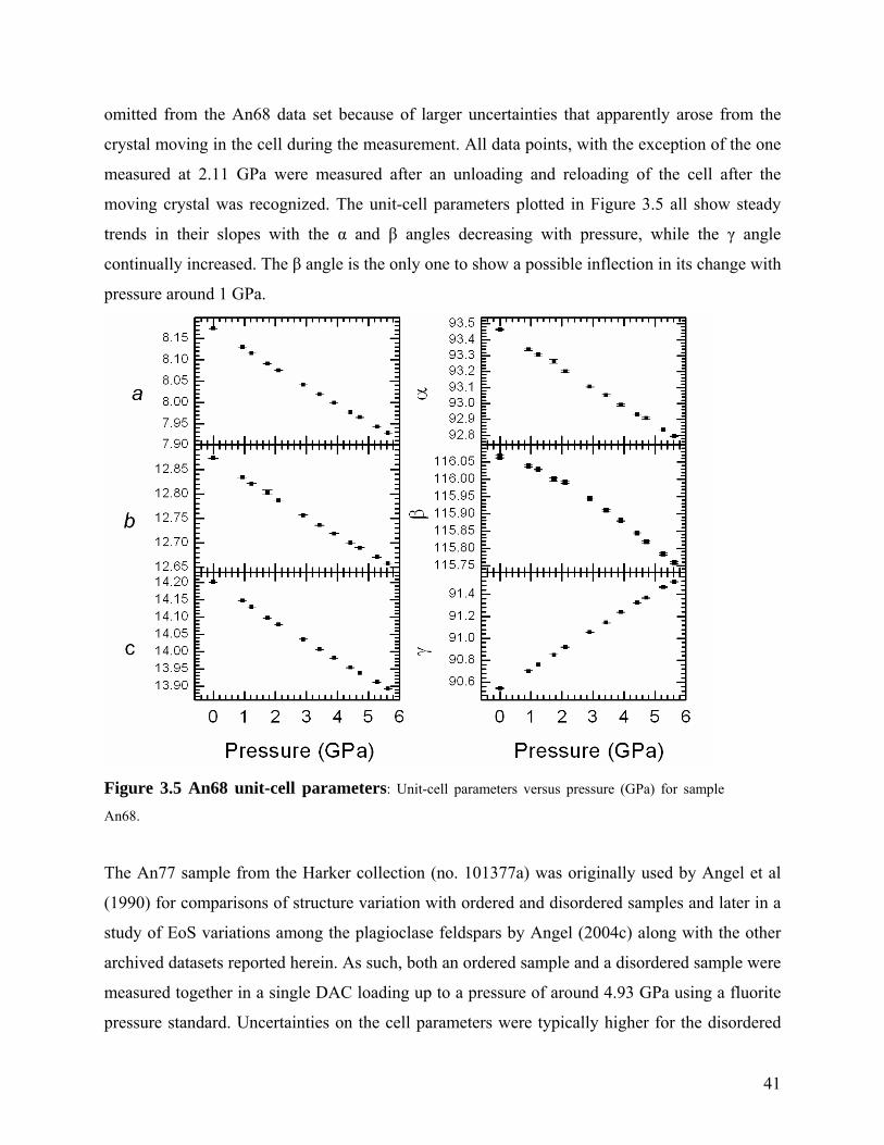
omitted from the An68 data set because of larger uncertainties that apparently arose from the

crystal moving in the cell during the measurement. All data points, with the exception of the one

measured at 2.11 GPa were measured after an unloading and reloading of the cell after the

moving crystal was recognized. The unit-cell parameters plotted in Figure 3.5 all show steady

trends in their slopes with the α and β angles decreasing with pressure, while the γ angle

continually increased. The β angle is the only one to show a possible inflection in its change with

pressure around 1 GPa.

Figure 3.5 An68 unit-cell parameters: Unit-cell parameters versus pressure (GPa) for sample

An68.

The An77 sample from the Harker collection (no. 101377a) was originally used by Angel et al

(1990) for comparisons of structure variation with ordered and disordered samples and later in a

study of EoS variations among the plagioclase feldspars by Angel (2004c) along with the other

archived datasets reported herein. As such, both an ordered sample and a disordered sample were

measured together in a single DAC loading up to a pressure of around 4.93 GPa using a fluorite

pressure standard. Uncertainties on the cell parameters were typically higher for the disordered

41

sample then the ordered one, but no peak broadening or crystal movement was reported for the

experiment. A second cell loading with just the disordered sample and fluorite was used to add

two data points between 0 and 2.5 GPa, and 2 data points above 4.9 GPa up to 6.31 GPa to the

disordered data set for leverage in fitting an EoS. The trends in both the ordered and disordered

samples were similar to those observed in the An68 data set (Figure 3.6).

Figure 3.6 An77 unit-cell parameters: Unit-cell parameter trends versus pressure for An77 for the

disordered sample (top) and the ordered sample (bottom).

42

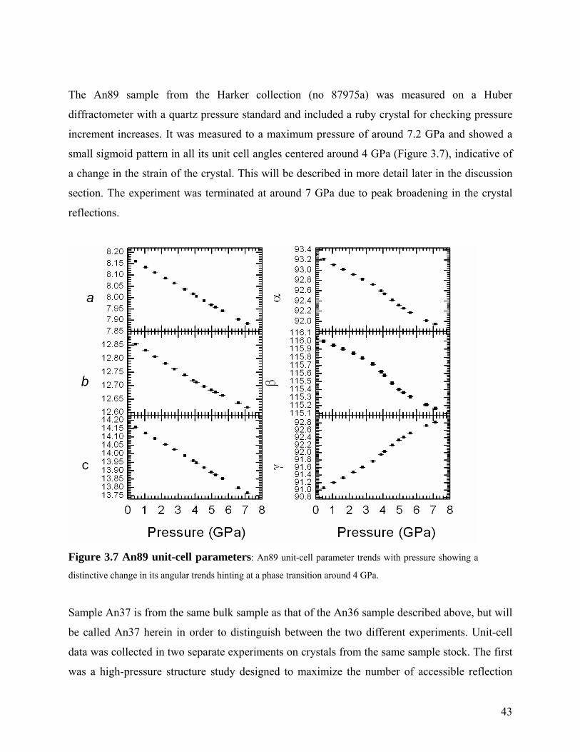
The An89 sample from the Harker collection (no 87975a) was measured on a Huber

diffractometer with a quartz pressure standard and included a ruby crystal for checking pressure

increment increases. It was measured to a maximum pressure of around 7.2 GPa and showed a

small sigmoid pattern in all its unit cell angles centered around 4 GPa (Figure 3.7), indicative of

a change in the strain of the crystal. This will be described in more detail later in the discussion

section. The experiment was terminated at around 7 GPa due to peak broadening in the crystal

reflections.

Figure 3.7 An89 unit-cell parameters: An89 unit-cell parameter trends with pressure showing a

distinctive change in its angular trends hinting at a phase transition around 4 GPa.

Sample An37 is from the same bulk sample as that of the An36 sample described above, but will

be called An37 herein in order to distinguish between the two different experiments. Unit-cell

data was collected in two separate experiments on crystals from the same sample stock. The first

was a high-pressure structure study designed to maximize the number of accessible reflection

43

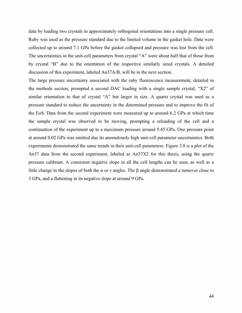
data by loading two crystals in approximately orthogonal orientations into a single pressure cell.

Ruby was used as the pressure standard due to the limited volume in the gasket hole. Data were

collected up to around 7.1 GPa before the gasket collapsed and pressure was lost from the cell.

The uncertainties in the unit-cell parameters from crystal “A” were about half that of those from

by crystal “B” due to the orientation of the respective similarly sized crystals. A detailed

discussion of this experiment, labeled An37A/B, will be in the next section.

The large pressure uncertainty associated with the ruby fluorescence measurement, detailed in

the methods section, prompted a second DAC loading with a single sample crystal, “X2” of

similar orientation to that of crystal “A” but larger in size. A quartz crystal was used as a

pressure standard to reduce the uncertainty in the determined pressure and to improve the fit of

the EoS. Data from the second experiment were measured up to around 6.2 GPa at which time

the sample crystal was observed to be moving, prompting a reloading of the cell and a

continuation of the experiment up to a maximum pressure around 9.45 GPa. One pressure point

at around 0.02 GPa was omitted due its anomalously high unit-cell parameter uncertainties. Both

experiments demonstrated the same trends in their unit-cell parameters. Figure 3.8 is a plot of the

An37 data from the second experiment, labeled as An37X2 for this thesis, using the quartz

pressure calibrant. A consistent negative slope in all the cell lengths can be seen, as well as a

little change in the slopes of both the α or γ angles. The β angle demonstrated a turnover close to

3 GPa, and a flattening in its negative slope at around 9 GPa.

44

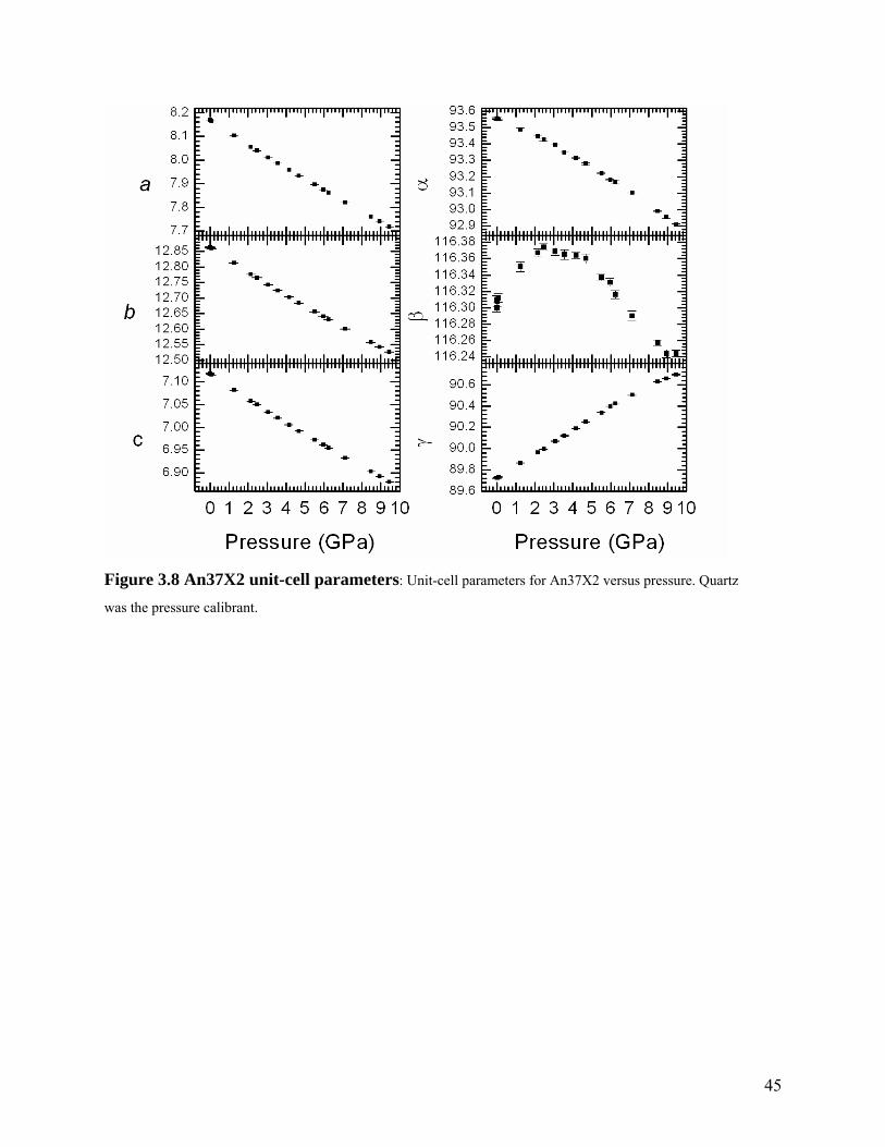
Figure 3.8 An37X2 unit-cell parameters: Unit-cell parameters for An37X2 versus pressure. Quartz

was the pressure calibrant.

45

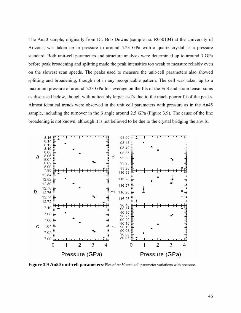
The An50 sample, originally from Dr. Bob Downs (sample no. R050104) at the University of

Arizona, was taken up in pressure to around 5.23 GPa with a quartz crystal as a pressure

standard. Both unit-cell parameters and structure analysis were determined up to around 3 GPa

before peak broadening and splitting made the peak intensities too weak to measure reliably even

on the slowest scan speeds. The peaks used to measure the unit-cell parameters also showed

splitting and broadening, though not in any recognizable pattern. The cell was taken up to a

maximum pressure of around 5.23 GPa for leverage on the fits of the EoS and strain tensor sums

as discussed below, though with noticeably larger esd’s due to the much poorer fit of the peaks.

Almost identical trends were observed in the unit cell parameters with pressure as in the An45

sample, including the turnover in the β angle around 2.5 GPa (Figure 3.9). The cause of the line

broadening is not known, although it is not believed to be due to the crystal bridging the anvils.

Figure 3.9 An50 unit-cell parameters: Plot of An50 unit-cell parameter variations with pressure.

46

The An60 sample, from a labradorite from the Smithsonian, was sent to the Virginia Tech

Crystallography Lab by Dr. Brown at the University of Washington. Using a quartz crystal for a

pressure standard, it was taken up in a DAC to a maximum pressure of 9.45 GPa with

measurements close to 0.5 GPa intervals. As in Figure 3.10, it displays the same trend as the

An50 but with the β-angle turnover occurring around 1 GPa and steadily decreasing up to the

maximum pressure. As noted above, this behavior is intermediate between that of the An50 and

the An68 samples. A few pressure points with high uncertainties were attributed to continued

gasket relaxation and therefore re-measured with significant improvement in all parameter

uncertainties; only the re-measured data are reported and used in this thesis.

Figure 3.10 An60 unit-cell parameters: Unit-cell parameters for An60 versus increasing pressure

(GPa).

Lastly, An96, from the “Miyake” locality in Japan, from the personal collection of Bernard

Evans (University of Washington), was measured up to around 5.18 GPa using a quartz crystal

as a pressure calibrant. The unit-cell parameters plotted in Figure 3.11 follow the general trends

47

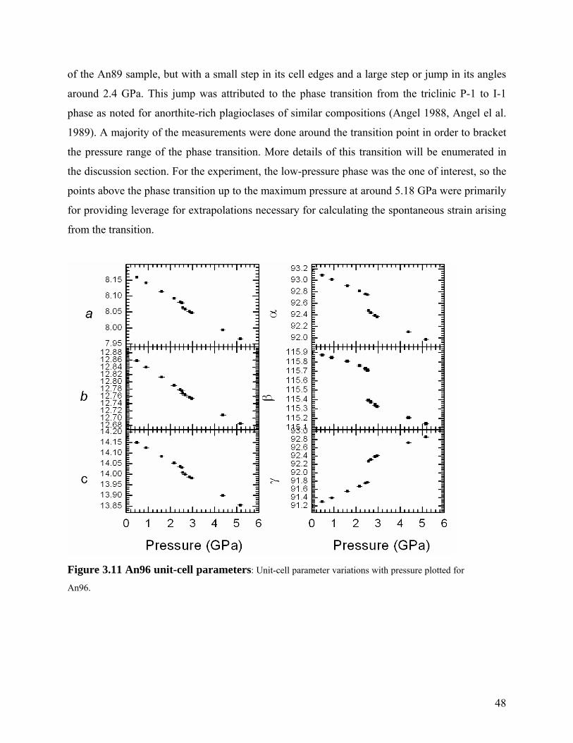
of the An89 sample, but with a small step in its cell edges and a large step or jump in its angles

around 2.4 GPa. This jump was attributed to the phase transition from the triclinic P-1 to I-1

phase as noted for anorthite-rich plagioclases of similar compositions (Angel 1988, Angel el al.

1989). A majority of the measurements were done around the transition point in order to bracket

the pressure range of the phase transition. More details of this transition will be enumerated in

the discussion section. For the experiment, the low-pressure phase was the one of interest, so the

points above the phase transition up to the maximum pressure at around 5.18 GPa were primarily

for providing leverage for extrapolations necessary for calculating the spontaneous strain arising

from the transition.

Figure 3.11 An96 unit-cell parameters: Unit-cell parameter variations with pressure plotted for

An96.

48

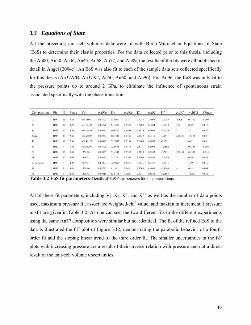
3.3 Equations of State

All the preceding unit-cell volumes data were fit with Birch-Murnaghan Equations of State

(EoS) to determine their elastic properties. For the data collected prior to this thesis, including

the An00, An20, An36, An45, An68, An77, and An89, the results of the fits were all published in

detail in Angel (2004c). An EoS was also fit to each of the sample data sets collected specifically

for this thesis (An37A/B, An37X2, An50, An60, and An96). For An96, the EoS was only fit to

the pressure points up to around 2 GPa, to eliminate the influence of spontaneous strain

associated specifically with the phase transition.

Composition Fit N Pmax Vo esdVo Ko esdKo K' esdK' K'' esdK'' wchi^2 ∆Pmax

0 BM4 13 5.23 664.7804 0.08101 52.8909 1.077 7.9288 1.4065 -2.2756 -0.008 0.1717 -0.006

20 BM4 12 8.23 667.88442 0.06798 61.2402 0.5242 5.6408 0.3694 -0.9438 0.14 0.49 0.017

36 BM3 10 5.59 669.01483 0.06822 69.6712 0.6894 3.1874 0.3049 -0.0536 -- 2.21 0.037

37X2 BM4 17 9.46 669.01807 0.05087 68.7648 0.4768 3.8939 0.3116 -0.4071 0.08721 1.5575 0.02

45 BM3 11 7.36 668.46122 0.04092 72.7832 0.3199 2.6909 0.1052 -0.059 0.82 0.03

50 BM3 9 5.24 669.11209 0.04129 72.9505 0.4388 2.877 0.2091 -0.0552 -- 0.2444 -0.008

60 BM4 16 9.48 1339.88 0.05965 73.4348 0.3555 4.2159 0.2243 -0.583 0.06458 0.4351 -0.014

68 BM3 10 5.63 1339.02 0.06325 75.3716 0.4392 3.3506 0.1937 -0.0486 -- 0.29 0.026

77 (ordered) BM3 8 4.93 1339.21 0.07023 76.9098 0.5248 3.3835 0.2726 -0.0475 -- 1.29 0.015

89 BM3 7 3.41 1338.96 0.08793 81.59 0.648 2.3708 0.4646 -0.1094 -- 0.18 0.004

96 BM3 6 2.44 1339.43 0.09419 83.8191 1.1029 2.33 0.8841 -0.0597 -- 1.6209 0.012

Table 3.2 EoS fit parameters: Details of EoS fit parameters for all compositions.

All of these fit parameters, including V0, K0, K’, and K’’ as well as the number of data points

used, maximum pressure fit, associated weighted-chi2 value, and maximum incremental pressure

misfit are given in Table 3.2. As one can see, the two different fits to the different experiments

using the same An37 composition were similar but not identical. The fit of the refined EoS to the

data is illustrated the f-F plot of Figure 3.12, demonstrating the parabolic behavior of a fourth

order fit and the sloping linear trend of the third order fit. The smaller uncertainties in the f-F

plots with increasing pressure are a result of their inverse relation with pressure and not a direct

result of the unit-cell volume uncertainties.

49

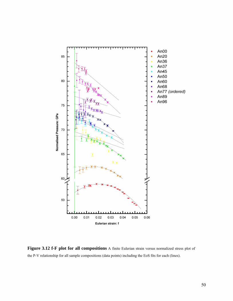
Figure 3.12 f-F plot for all compositions A finite Eulerian strain versus normalized stress plot of

the P-V relationship for all sample compositions (data points) including the EoS fits for each (lines).

50

3.4 Compliance Tensor Sums

In addition to the EoS for each sample composition, the compliance tensor sums were also

calculated from the unit-cell parameter variation with pressure using the WinStrain program and

the Brown et al. (2006) axial conventions as detailed in the Chapter 2. All values are in terms of

GPa-1. The calculated compliance tensor sums can be found in Appendix B.

Some general trends hold for the derived values over the range of compositions considered. The

relationship defined for linear compressibility, where a negative strain over a pressure interval

yields a positive compliance tensor sum, causes the compliance tensor sums corresponding to the

diagonal terms of the elastic strain moduli ( 1ε , 2ε , 3ε ) to be always positive for a positive

pressure interval because the associated strain is always negative, or compressional. The off-

diagonal elastic strain components ( 4ε , 5ε , 6ε ) however tend to vary with the unit cell angles,

where 4ε scales with α, 5ε with β, and 6ε with γ, and can have either positive and negative

trends with pressure. A positive angle increase results in a negative strain and, thus, relates to a

positive compliance tensor sum. Following the same relation, a negative angle change should

give a negative compliance tensor sum. So, for the compliance tensor sums for each composition

of intermediate plagioclase calculated, the diagonal terms will always be positive and the off-

diagonal terms will vary and depend on the trend of the unit-cell angles.

For example, as illustrated in Figure 3.13 of the An37X2 compliance tensor sums, the α-angle

continually decreases and the γ-angle always increases, 4ε is always negative and 6ε is always

positive. However because of the turnover in the β-angle, 5ε is always negative but shows a

positive trend in its values in excess of about 7 GPa. All the compressional terms are positive

over the entire pressure interval.

51

Figure 3.12 An37X2 unit-cell parameters with compliance tensor sums: An37X2

compliance tensor sums plotted versus pressure (bottom) along with their influencing unit-cell parameters

(top) to show the correlation of sign trends.

The uncertainty applied to each derived compliance tensor sum for each interval used was

calculated through the propagation of errors of the associated pressure uncertainties alone. In a

manual calculation it was found that the contribution to the overall uncertainty by the

propagation of unit-cell parameters through the strain tensor component calculations was not

significant in comparison to that of the pressure uncertainties. The manual method involved

calculating the strain tensor components for all possible variations in the unit-cell parameter

within their uncertainties and finding the largest shift in each strain tensor component away from

the calculated value. These values were, on average, an order of magnitude, or more, smaller

than that found by simply propagating the error in the pressure values.

52

The compliance tensor sums were plotted, with their estimated uncertainties, versus the

incremental pressure midpoints and appropriately fit in order to extrapolate the sums of the

tensor components back to zero pressure. These values were used in calculations of the full

compliance tensor for some compositions, as will be detailed in Chapter 4. Because there is no

symmetry constraint on the type of fit applied to the terms derived from triclinic systems, their

variations with pressure were fit with the fewest possible parameters using the linear-least

squares method. Uncertainties for each of the tensor component sums were used as weights and

either a linear or parametric equation was fit to the data, where appropriate, to give compliance

tensor sums estimated at room pressure.

The room pressure compliance tensor sums, as well as their calculated uncertainties, were

independently verified though the calculation of linearized Equations of State for each

composition along primary orthogonal axes - following the coordinate basis system of Brown et

al. (2006) - to equate them on the same axial system with the compliance tensor sums. The K0

parameter refined in a linearized EoS is one-third of the inverse of the linear compressibility at

room pressure (Angel 2000). This allows for the direct comparison between the K0 parameters of

linearized EoS fits of the d(100) plane spacing and the b-axis unit-cell parameter with the

compliance tensor sums of s11+s12+s13 and s21+s22+s23 related to each of these axes, respectively,

because the compressional terms are affected only by the resolved strains along the primary axis

directions. The remaining compressional compliance tensor sum of s31+s32+s33 can not be

directly compared to the c-axis as it is not fixed to that specified direction in the chosen

coordinate system, but is arbitrarily assigned to satisfy the right-hand rule.

The “linear-K0” parameter for the fits of the d(100) spacing and the b-axis unit-cell parameter for

each composition, when compared to the related compliance tensor sums, were within 10-3 of

each other in actual value. Small discrepancies are likely the result of pressure averaging in the

compliance tensor sum calculations, fit inconsistencies associated with varying degrees of data

scatter for different compositions, etc.

The uncertainties of the K0 parameters refined in a linearized EoS fits along the a*-, b-, and c-

axis directions are good approximations of the uncertainties of each of the diagonal

compressional terms in the elastic moduli sums determined at room pressure. I found that the

values for the uncertainties in the K0 terms of the linearized EoS for each of the different

compositions is of the same order of magnitude or one larger than those calculated for any of the

53

compliance component sums. This verifies that the assigned uncertainties to the compliance

sums are adequate and not overly under or overestimated. Also for each composition, the volume

compressibility derived from the averaging of the K0 terms for all three primary axis directions is

equal to that derived from the sum of 1ε + 2ε + 3ε within the uncertainties.

3.5 Structure

Two separate structural data suites were collected in conjunction with measurement of the unit-

cell parameters with pressure for the An37 sample, one was on the experiment with two

differently oriented crystals in the same DAC with a ruby pressure calibrant and the other was on

the experiment with a single sample crystal and a quartz pressure calibrant. These will be labeled

An37A/B and An37X2, respectively, from here-on to distinguish between them. The structural

data for both experiments were collected using the Xcalibur-1 single crystal X-ray diffractometer

described in detail in the Chapter 2 of this thesis. The data were integrated with the WinIntegrStp

program (Angel 2003), reduced with the Absorb program (Angel 2004a), and refined using the

WinGX software (Farrugia 1999). Experimental details for both An37A/B and An37X2 with

their associated pressure interval are given in Appendix C. In both experiments the extra-

framework M cation site was treated as a split site between the Ca and Na constituents, where

each cation was allowed to refine independently of the other in terms of position and

displacement parameter. The refined parameters for each experiment, anisotropic displacement

parameters (when enough data were collected), atomic positions, and displacement parameters,

as well as the calculated tetrahedral bond lengths and associated bond angles are given in

Appendix C.

Due to the small size of the A and B sample crystals loaded simultaneously in the DAC for the

An37A/B high pressure experiment, there were too few reflections for a structure refinement

with reasonable parameter uncertainties when each was refined independently. As such, all

An37A/B structure refinements reported were refined using non-merged combined reflection

files. The An37X2 experiment, though containing a single crystal oriented similarly to that of

crystal A in the AN37A/B experiment, was of a large enough size to yield enough reflections for

structure refinement.

54

Chapter 4 Discussion

4.1 Chapter Introduction In this chapter the results found from unit-cell, structure, EoS and elasticity

measurements/calculations will be integrated to identify the underlying structural mechanisms

responsible for the variations identified across the solid solution series for albite to anorthite.

4.2 Cell Parameter Trends

Brown et al. (1984) noted that the topological similarities for all feldspar compositions give rise

to consistent trends in their unit cell parameters with variations in temperature, composition and

pressure. The major observations dealt with the thermal expansion effects on primarily

potassium feldspars. There were three distinct Trends, Trend I, Trend II and Trend III, noted and

typically separated by abrupt shifts in the unit cell parameters associated with a phase transition.

For the plagioclase solid solution series, Brown et al. (1984) observed a linear coupling between

an increase in the b- axis and a decrease in the c- axes for composition from An00 to around

An60 after which their relation plotted as a decoupled vertical line where only the c- axis

continued to decrease, with no associated shift in the angles. Utilizing the limited database of

experiments conducted with feldspars at high pressure at the time of publication (Bridgman

1928, Hazen 1976, Hazen and Prewitt 1977, Wright and Stewart 1968), it was also noted that

most followed the reverse of Trend I (compression over expansion), where there is coupled

decrease in both b- and c-axes, a decrease in the a-axis and α-angle, no decrease of γ, and an

increase in the β-angle.

The current data show some but not all of these observed trends. A plot of b- versus c-

dimensions for all compositions at room pressure (Figure 4.1) shows the same linear to vertical

shift between An00 and An100, with the turnover near An60 as seen by Brown et al. (1984). It

also shows the general slope of the axial relations with increasing pressure following the reverse

55

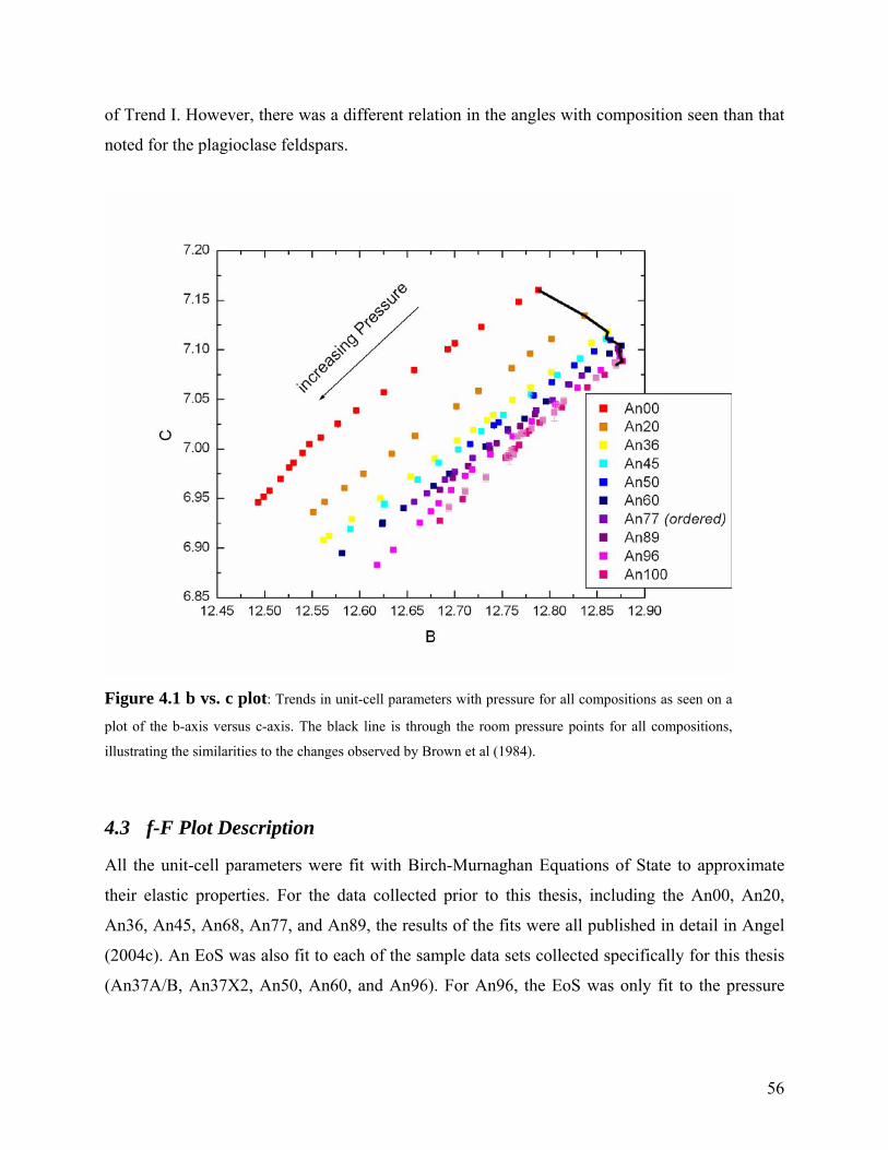
of Trend I. However, there was a different relation in the angles with composition seen than that

noted for the plagioclase feldspars.

Figure 4.1 b vs. c plot: Trends in unit-cell parameters with pressure for all compositions as seen on a

plot of the b-axis versus c-axis. The black line is through the room pressure points for all compositions,

illustrating the similarities to the changes observed by Brown et al (1984).

4.3 f-F Plot Description

All the unit-cell parameters were fit with Birch-Murnaghan Equations of State to approximate

their elastic properties. For the data collected prior to this thesis, including the An00, An20,

An36, An45, An68, An77, and An89, the results of the fits were all published in detail in Angel

(2004c). An EoS was also fit to each of the sample data sets collected specifically for this thesis

(An37A/B, An37X2, An50, An60, and An96). For An96, the EoS was only fit to the pressure

56

points up to around 2 GPa to eliminate any influence of spontaneous strain associated

specifically with the phase transition.

Illustrated in the f-F plot of Figure 3.13, the trend from compositions An00 to An20, both fit with

fourth-order expansions of the Birch-Murnaghan EoS, is for a turnover from an initially

increasing to a decreasing slope. This reflects the change over in the K’ values from those greater

than 4 to those less than 4, weighted down by the very large negative value of K’’ of the fit. The

restricted third-order Birch-Murnaghan fit to the data, for each composition, suggests an average

K’ around 5.8 (Angel 2004c).

For compositions from An 37 to An77 this turnover is not evident within the measurable

pressure range. Much of the data originally collected by Angel (2004c) were fit best with a 3rd

order EoS and not a 4th order EoS necessary to see the turnover in the K values. The larger

uncertainties from fluorite or ruby pressure standards, lack of data coverage, or the actual lack of

a turnover in the data trend would all account for this observation. Within the An37 to An77

range only An37X2 and An60 were adequately described by fourth-order fits but the turnover is

either outside the lower pressure range, as is the case for An37X2 or at extremely low pressures,

as is the case for An60 (K’ = 4 at 0.36 GPa, K’’ turnover at 3.03 GPa). In general the trend in

this compositional range is for a moderate downward linear trend in the f-F plot, characteristic of

an average K’ value of around 3.2 as noted by Angel (2004c).

At the anorthite-rich end of the plagioclase solid solution series, the EoS fit for the An89 and

An96 data were both complicated by phase transitions between 3 and 4 GPa. Each was fit with

3rd order EoS to the data range below their respective phase transitions. This resulted in much

steeper downward sloping linear lines on the f-F plot than those for the more intermediate

compositions fit with the same order equation. Their general slope is very similar to that of

An00, An20, An37 and An60 at higher pressures after the decrease in their K values below 4.

Angel (2004c) predicted that the turn-over in the EoS fit from a positive to a negative trending

slope on the f-F plot would occur within metamorphic grade P-T conditions in the more

intermediate compositions between about An20 and An40. Overall, Figure 3.13 demonstrates

this general change in slope across the whole series, but the data scatter is still too great to pick

out where the turnover occurs exactly.

57

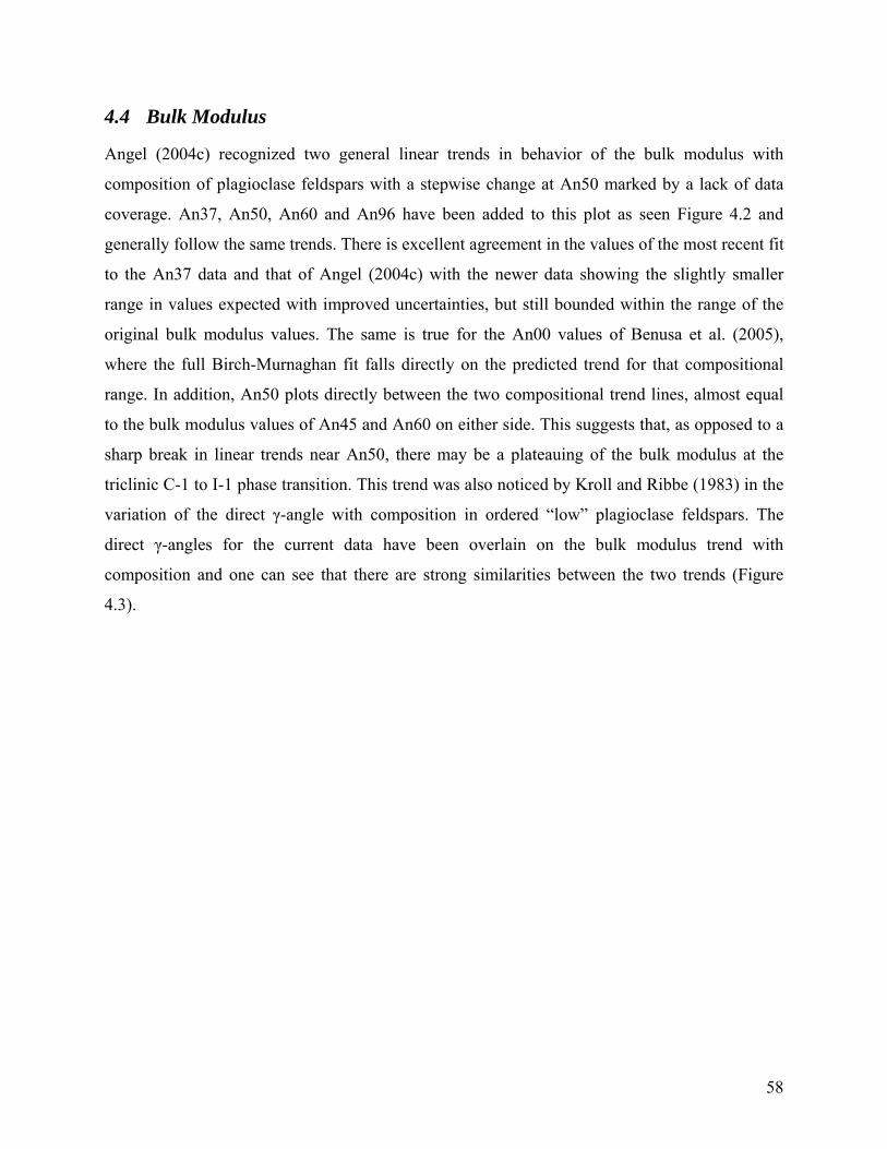
4.4 Bulk Modulus

Angel (2004c) recognized two general linear trends in behavior of the bulk modulus with

composition of plagioclase feldspars with a stepwise change at An50 marked by a lack of data

coverage. An37, An50, An60 and An96 have been added to this plot as seen Figure 4.2 and

generally follow the same trends. There is excellent agreement in the values of the most recent fit

to the An37 data and that of Angel (2004c) with the newer data showing the slightly smaller

range in values expected with improved uncertainties, but still bounded within the range of the

original bulk modulus values. The same is true for the An00 values of Benusa et al. (2005),

where the full Birch-Murnaghan fit falls directly on the predicted trend for that compositional

range. In addition, An50 plots directly between the two compositional trend lines, almost equal

to the bulk modulus values of An45 and An60 on either side. This suggests that, as opposed to a

sharp break in linear trends near An50, there may be a plateauing of the bulk modulus at the

triclinic C-1 to I-1 phase transition. This trend was also noticed by Kroll and Ribbe (1983) in the

variation of the direct γ-angle with composition in ordered “low” plagioclase feldspars. The

direct γ-angles for the current data have been overlain on the bulk modulus trend with

composition and one can see that there are strong similarities between the two trends (Figure

4.3).

58

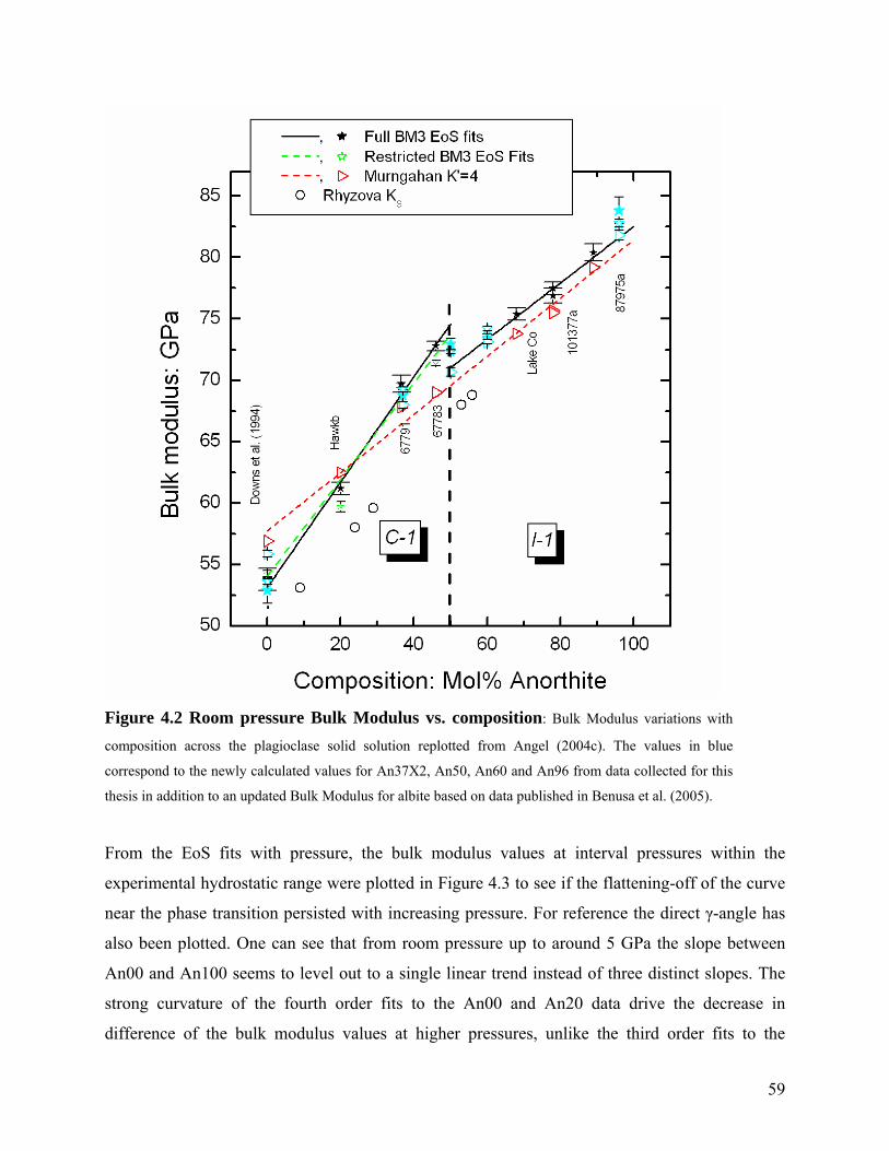
Figure 4.2 Room pressure Bulk Modulus vs. composition: Bulk Modulus variations with

composition across the plagioclase solid solution replotted from Angel (2004c). The values in blue

correspond to the newly calculated values for An37X2, An50, An60 and An96 from data collected for this

thesis in addition to an updated Bulk Modulus for albite based on data published in Benusa et al. (2005).

From the EoS fits with pressure, the bulk modulus values at interval pressures within the

experimental hydrostatic range were plotted in Figure 4.3 to see if the flattening-off of the curve

near the phase transition persisted with increasing pressure. For reference the direct γ-angle has

also been plotted. One can see that from room pressure up to around 5 GPa the slope between

An00 and An100 seems to level out to a single linear trend instead of three distinct slopes. The

strong curvature of the fourth order fits to the An00 and An20 data drive the decrease in

difference of the bulk modulus values at higher pressures, unlike the third order fits to the

59

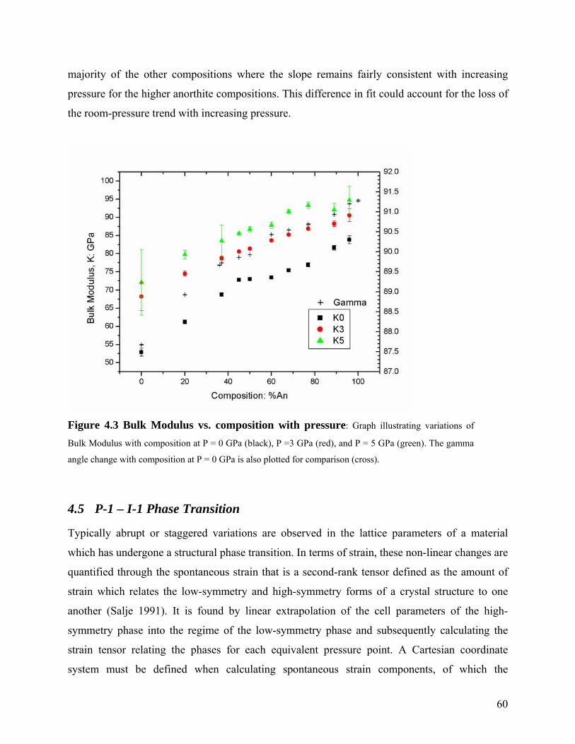
majority of the other compositions where the slope remains fairly consistent with increasing

pressure for the higher anorthite compositions. This difference in fit could account for the loss of

the room-pressure trend with increasing pressure.

Figure 4.3 Bulk Modulus vs. composition with pressure: Graph illustrating variations of

Bulk Modulus with composition at P = 0 GPa (black), P =3 GPa (red), and P = 5 GPa (green). The gamma

angle change with composition at P = 0 GPa is also plotted for comparison (cross).

4.5 P-1 – I-1 Phase Transition

Typically abrupt or staggered variations are observed in the lattice parameters of a material

which has undergone a structural phase transition. In terms of strain, these non-linear changes are

quantified through the spontaneous strain that is a second-rank tensor defined as the amount of

strain which relates the low-symmetry and high-symmetry forms of a crystal structure to one

another (Salje 1991). It is found by linear extrapolation of the cell parameters of the high-

symmetry phase into the regime of the low-symmetry phase and subsequently calculating the

strain tensor relating the phases for each equivalent pressure point. A Cartesian coordinate

system must be defined when calculating spontaneous strain components, of which the

60

coordinate system of Brown et al. (2006) was used in this thesis. Uncertainties in the calculated

values can arise from uncertainties in the low-symmetry cell parameters, the pressure

measurements, or the extrapolated cell-parameters (Angel 2000).

The spontaneous strain tensor is symmetric with six independent components like the actual

strain tensor, and similarly can be reduced to either a volumetric spontaneous strain or a scalar

spontaneous strain. The volumetric spontaneous strain can be found by fitting a Murnaghan EoS,

which is usually sufficient for estimating the correct bulk modulus for materials with up to 10%

compressibility, to the high symmetry phase data. Because of the large weighting of the V0 and

K0 parameters in the EoS fit, the high symmetry phase is usually fit to an adjusted pressure scale,

which subtracts off a constant reference pressure for each utilized data point, in order to avoid

large instabilities in the fit.

The scalar strain as defined by Redfern and Salje (1987) and Salje (1993) is given as:

( ) ( )22 ∑∑= iis oree ε Equation 4.1

Where εi are the three components of the strain ellipsoid along its three principle directions and ei

are the six components of the spontaneous strain tensor. Both give similar calculated values and

are measures of the spontaneous strain independent of any sign convention on the actual

component values.

Using high-pressure single-crystal X-ray diffraction techniques to calculate the spontaneous

strain provides very precise unit-cell measurements, well-defined applied stresses, and typically

unambiguous determination of the crystal orientation in all phases (Angel 2000). Measurement

of the unit-cell parameters for both phases over a large pressure interval helps ensure adequate

leverage of the extrapolated data outside its normal stability range and establishes a baseline to

account for the smaller amounts of strain not dependent on the structural phase transition (Salje

1991). For most solids under pressure, the spontaneous strain displays a complicated non-linear

behavior due to increased opposing inter-atomic forces as the atoms are compressed together

(Carpenter et al. 1998, Angel 2000).

Independent confirmations of the accuracy of the extrapolated values can be done by means of

parallel calculations with different functions (e.g. Boffa-Ballaran et al. 2000), comparison

between the unit-cell volumes extrapolated from the unit-cell parameters and those of the actual

61

volume EoS fit, and by extrapolating the high-symmetry values prior to transforming them to the

low-symmetry phase setting.

The two compositions observed for this thesis to undergo the P-1 to I-1 phase transition typical

of very anorthite-rich plagioclase were An89 and An96. Figure 4.4 shows the spontaneous strain

each tensor component for both An89 and An96. The large values associated with the off-

diagonal shear components for An89 and An96 compared with the smaller values for the

diagonal compressional components are consistent with the unit cell parameter changes seen

associated with the structural phase transition which show large variations in the angular terms

but only slight discontinuities in the unit cell lengths. The signs of the terms are also consistent

with that of the unit cell parameter changes. For example, the positive change in α corresponds to

a negative trend in the e4 parameter due to the negative sign in the strain tensor equation.

62

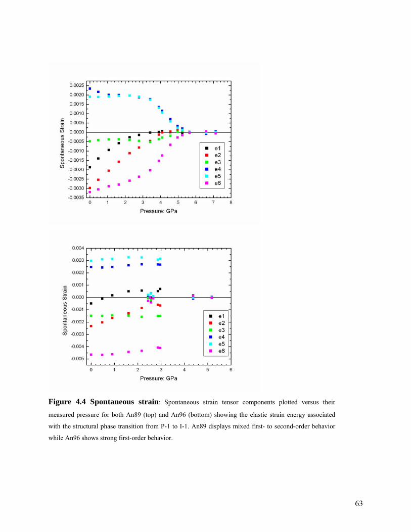
Figure 4.4 Spontaneous strain: Spontaneous strain tensor components plotted versus their

measured pressure for both An89 (top) and An96 (bottom) showing the elastic strain energy associated

with the structural phase transition from P-1 to I-1. An89 displays mixed first- to second-order behavior

while An96 shows strong first-order behavior.

63

The strong first order nature of the trend of the An96 phase transition (Figure 4.4) is consistent

with that of the Monte Somma sample used by Angel et al. (1989) of almost equivalent

composition. This was attributed to a difference between the potential well of the Ca-site

between the high-pressure and high-temperature I-1 phases, which effectively renormalizes the

effective coefficient on the fourth-order term in the Landau free-energy expansion to the Na-

content in the structure (Angel et al. 1989). However the more gradual change in the spontaneous

strain of An89 is approaching the trend observed in a second order phase transition. Angel et al.

(1989) predicted this behavior for compositions with higher Na content, determining that the

nature of the phase transition would trend away from first-order through tricritical to second-

order behavior accompanied by similar changes in the behavior of the physical properties and

elastic constants.

These can be seen more clearly in Figure 4.5 which plots the scalar spontaneous strain of both

An89 and An96 versus pressure. It should be noted that the values of both the spontaneous strain

and scalar strain calculated for An96 were significantly lower than those of the Angel et al.

(1989) Monte Somma sample (a low symmetry phase scalar spontaneous strain of 65 for An96

compared to 100 for the Monte Somma sample). The phase transition from P-1 to I-1 also

occurred in An96 at a lower pressure (2.5 over 2.8 GPa) than predicted previously. These

differences could be due to compositional differences between samples, given the range provided

by the microprobe results. It should be noted that the older data have greater pressure

uncertainties due to use of fluorite and ruby as the primary pressure calibrants. Also, the extra

inflection seen in the spontaneous strain for An89 below 2 GPa is most likely not a real feature

but an artifact of the linear fit to limited high phase data points and falls well within the range of

uncertainties for the extrapolation.

64

Figure 4.5 Scalar spontaneous strain: Scalar spontaneous strain versus pressure plotted for both

An89 (top) and An96 (left) to clearly illustrate the overall trend of the P-1 to I-1 phase transition observed

in both sample compositions.

The thermodynamic nature of the P-1 ↔ I-1 phase transition is such that the associated order

parameter is sensitive to the degree of Al/Si ordering within the structure, so that the description

of the volume behavior with pressure or temperature depends on two coupled order parameters;

Q for the displacive P-1 ↔ I-1 transition, and QOD for the Al/Si ordering arising from the C-1

I-1 phase transition (Carpenter 2006, and references therein). The Bulk Modulus is predicted to

scale linearly with QOD2, following Equation (16) in Carpenter (2006). Carpenter (2006) plotted

data from Hackwell and Angel (1992) and Angel (1994) for end-member anorthite of differing

states of order in both the low-pressure P-1 phase and high-pressure I-1 phase. Carpenter (2006)

65

observed the direct correlation between K and QOD2 predicted by Landau theory, but with two

different sloping trends between the P-1 and I-1 phases, crossing near natural anorthite (QOD =

0.92). Without quantifying the influence of the displacive transition on the order parameter, or

taking into account other effects, little more can be concluded given the great simplification of

the K values used.

Table 4.1 Order parameters: Order

parameters for all compositions with

corresponding Bulk Modulus values

where K’ =4. Sample Qod K1 esd

An00 0.92 56.9 0.3

An20 -- 62.5 0.2

An36 -- 67.8 0.3

An37X2 0.33 68.0 0.3

An45 -- 69.0 0.5

An50 0.27 70.7 0.3

An60 0.09 73.1 0.2

An68 0.56 73.8 0.2

An77o 0.72 75.7 0.2

An77d 0.48 75.7 0.2

An89 0.85 79.2 0.2

An96 0.90 81.8 0.4

Notes.

The reference state for An00 to An50 is C-1,

from An60 to An77 it is I-1 and for An89 to

An96 it is P-1

Table 4.1 lists the values of K0 for the Murnaghan EoS, with a K’ = 4, fit to the data in this thesis

together with QOD values obtained from structure refinements (Angel et al. 1992, and this thesis).

When plotted in Figure 4.6, this data shows that with more albite-rich compositions, the low-

pressure I-1 data plot consistently along the P-1 trend extrapolated from end-member anorthite

for all states of Al/Si order. This suggests that the difference in the two trends is not the result of

the P-1 ↔ I-1 transition. Instead, it is likely that the values for the bulk moduli of the high-

66

pressure I-1 phasesare unreliable due to the smeared nature of the phase transition with

decreasing QOD as is seen in the data for An89. In particular, as the transition becomes more

second-order in nature, the EoS fit with K’ = 4 becomes somewhat arbitrary, and probably biases

the value of K0.

Figure 4.6 Bulk Modulus vs. QOD

2: Bulk Modulus values (Murnaghan EoS fit with K’ = 4) versus QOD2

values as found in Angel (1992) with linear fits to K values in the low-pressure P-1 phase (black) and in the high-

pressure I-1 phase (red). Data for this thesis from An60 to An96 (green) have also been plotted.

4.6 Structure: An37 at high pressure

Benusa et al. (2005) published a detailed high pressure study on end-member albite, including

structural data up to 9.43 GPa. They found that the compressionial behavior of albite was not

attributed to the formation of new extra-framework cation bonds such as those observed in

microcline between K atoms and Obm atoms (Downs et al. 1999), as the Na-O bond distances

show a steady decrease with pressure. Also, albite showed only very small changes in the

average tetrahedral bond length over the entire measured pressure range. Instead, the anomalous

67

cell parameter trends observed for albite above about 5 GPa were interpreted to result from two

compression mechanisms. The initial dominant mechanism was noted as closure along the [100]

of the crankshafts, as evidenced by significant changes in the T-O-T bond angles of the rigid

tetrahedral framework, especially in the reduction of the T-Obo-T and T-Oco-T bond angles. At

higher pressures the tilting gave rise to the second compression mechanism, which was an

increased rate of shear in at least two of the four-membered tetrahedral rings, specifically the

T1o-T2o-T1m-T1m ring.

The structure of An37 was determined and refined in C-1 for this thesis up to a maximum

pressure around 9.5 GPa as described in Chapter 3. The extra-framework cation sites were

modeled as split Ca and Na sites, which refined to an average split distance around 0.7

Angstroms. The positional parameters and the displacement parameters of each of the two sites

were refined without constraints, so the resulting parameters and the bond lengths must be

treated with caution. There is also significant anisotropy in the displacement parameters of both

cation sites.

There were not enough data to refine the Al versus Si distribution within the An37 structure. The

Al-occupancy for each of the tetrahedral sites at room pressure can be calculated as a function of

the average T-O bond distances and mineral composition (Ribbe 1983) as:

( ) ( )13.0125.0

OTOTnt avgi

Ani−−−

+−= Equation 4.2

where ti is the estimated Al-content on a scale for 0 to 1, <Ti-O> is the average individual

tetrahedral distance, and <Tavg-O> is the grand mean tetrahedral distance for all tetrahedral sites.

The grand mean of all of the T-O bond lengths for An37 at room pressure is 1.656 Angstroms

which, following equation (2) of Angel et al. (1990) corresponds to the correct composition of

An37. Just under half of the total Al is concentrated on the preferred T1o site (t1o = 0.59)

compared to the other tetrahedral sites (t1m = 0.25, t2o = 0.27, and t2m = 0.27). This Al-

distribution in the structure is consistent with other intermediate low plagioclase structures, with

the majority of the Al concentrated on the preferred T1o site, and the remainder distributed

equally amongst the other three sites. If the state of order is calculated relative to the albite

ordering pattern using equation (7) of Angel et al. (1990) then the sample has a Qod = 0.33. This

68

apparently low state of order is actually typical of a “low” plagioclase and represents the

presence of at least some degree of local ordering on the anorthite pattern.

The degree of Si/Al ordering throughout the An37 is not assumed to have a significant affect on

variations seen with pressure based on the minimal difference in the unit-cell parameters with

pressure between ordered and disordered An77 (Figure 3.6). Also, the combined structural data

obtained from the An37 experiments shows very little variation in the T-O bond lengths with

pressure (see Appendix C), with an average variation of only 0.027 Angstroms over a 10 GPa

pressure range. As in albite, this would point to the primary mechanism as being other than

compression of the tetrahedra.

Also, as illustrated in Figure 4.7, the Na-O and Ca-O bond distances show fairly uniform

compression up to the maximum measured pressure and generally show similar trends as seen in

albite. For both Na-O and Ca-O, the shortest bonds are to Oa1, Oa2, Obo, and Odo, and the

distances and their behavior upon compression are very similar to those in albite itself. The

interpretation of the longer bond distances is made uncertain by the use of the split site

refinement for the Na/Ca extra-framework position. In comparison to albite, the Na-Odm appears

to be shortened in An37 and closer to what is considered a bonded interaction in albite (Downs et

al. 1999). The Ca-O distances appear to reflect a higher coordination number for Ca than for Na,

with the Ca-Obm and Ca-Ocm distances much shorter than the corresponding Na-O distances,

while the Odm has been removed from the coordination environment of Ca. This is consistent

with the 6 and 7 coordination found for Ca in end-member anorthite (e.g. Angel et al. 1990 and

references therein).

69

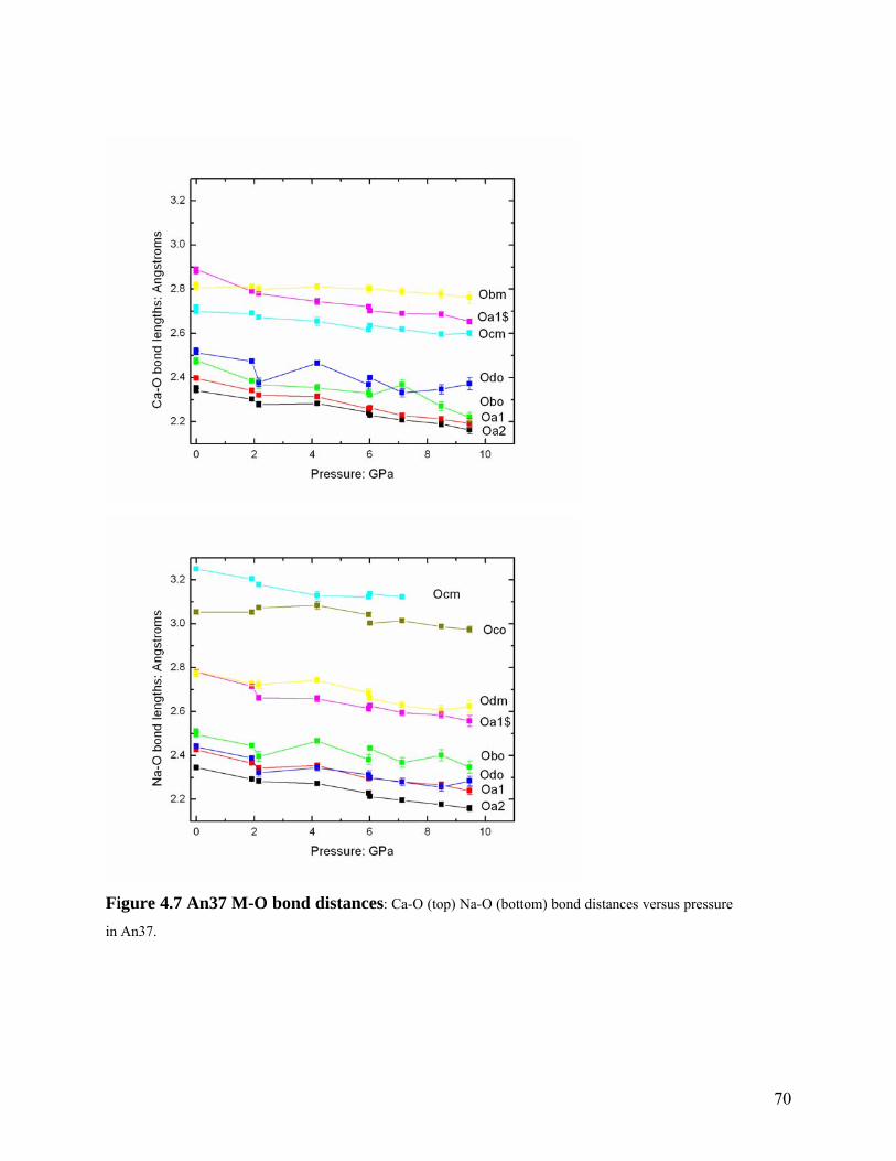
Figure 4.7 An37 M-O bond distances: Ca-O (top) Na-O (bottom) bond distances versus pressure

in An37.

70

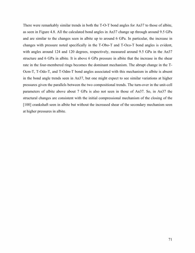
There were remarkably similar trends in both the T-O-T bond angles for An37 to those of albite,

as seen in Figure 4.8. All the calculated bond angles in An37 change up through around 9.5 GPa

and are similar to the changes seen in albite up to around 6 GPa. In particular, the increase in

changes with pressure noted specifically in the T-Obo-T and T-Oco-T bond angles is evident,

with angles around 124 and 120 degrees, respectively, measured around 9.5 GPa in the An37

structure and 6 GPa in albite. It is above 6 GPa pressure in albite that the increase in the shear

rate in the four-membered rings becomes the dominant mechanism. The abrupt change in the T-

Ocm-T, T-Odo-T, and T-Odm-T bond angles associated with this mechanism in albite is absent

in the bond angle trends seen in An37, but one might expect to see similar variations at higher

pressures given the parallels between the two compositional trends. The turn-over in the unit-cell

parameters of albite above about 7 GPa is also not seen in those of An37. So, in An37 the

structural changes are consistent with the initial compressional mechanism of the closing of the

[100] crankshaft seen in albite but without the increased shear of the secondary mechanism seen

at higher pressures in albite.

71

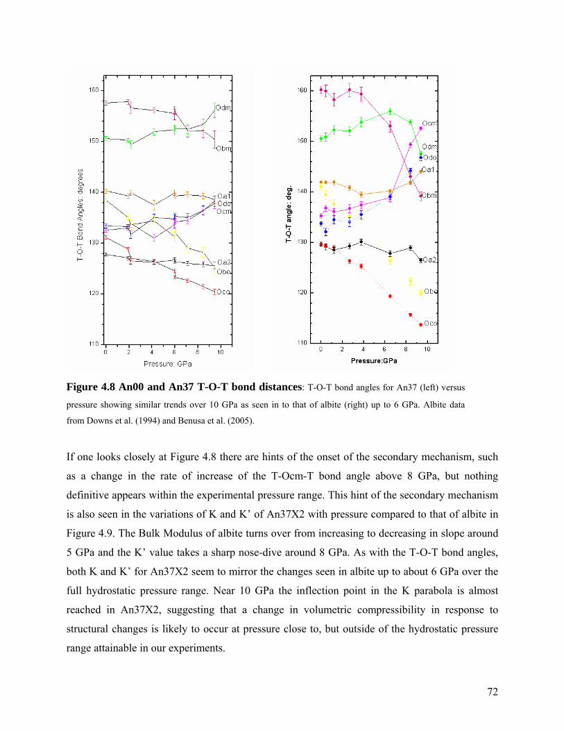
Figure 4.8 An00 and An37 T-O-T bond distances: T-O-T bond angles for An37 (left) versus

pressure showing similar trends over 10 GPa as seen in to that of albite (right) up to 6 GPa. Albite data

from Downs et al. (1994) and Benusa et al. (2005).

If one looks closely at Figure 4.8 there are hints of the onset of the secondary mechanism, such

as a change in the rate of increase of the T-Ocm-T bond angle above 8 GPa, but nothing

definitive appears within the experimental pressure range. This hint of the secondary mechanism

is also seen in the variations of K and K’ of An37X2 with pressure compared to that of albite in

Figure 4.9. The Bulk Modulus of albite turns over from increasing to decreasing in slope around

5 GPa and the K’ value takes a sharp nose-dive around 8 GPa. As with the T-O-T bond angles,

both K and K’ for An37X2 seem to mirror the changes seen in albite up to about 6 GPa over the

full hydrostatic pressure range. Near 10 GPa the inflection point in the K parabola is almost

reached in An37X2, suggesting that a change in volumetric compressibility in response to

structural changes is likely to occur at pressure close to, but outside of the hydrostatic pressure

range attainable in our experiments.

72

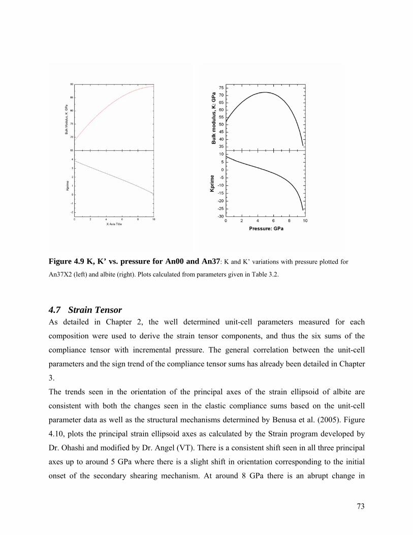
Figure 4.9 K, K’ vs. pressure for An00 and An37: K and K’ variations with pressure plotted for

An37X2 (left) and albite (right). Plots calculated from parameters given in Table 3.2.

4.7 Strain Tensor As detailed in Chapter 2, the well determined unit-cell parameters measured for each

composition were used to derive the strain tensor components, and thus the six sums of the

compliance tensor with incremental pressure. The general correlation between the unit-cell

parameters and the sign trend of the compliance tensor sums has already been detailed in Chapter

3.

The trends seen in the orientation of the principal axes of the strain ellipsoid of albite are

consistent with both the changes seen in the elastic compliance sums based on the unit-cell

parameter data as well as the structural mechanisms determined by Benusa et al. (2005). Figure

4.10, plots the principal strain ellipsoid axes as calculated by the Strain program developed by

Dr. Ohashi and modified by Dr. Angel (VT). There is a consistent shift seen in all three principal

axes up to around 5 GPa where there is a slight shift in orientation corresponding to the initial

onset of the secondary shearing mechanism. At around 8 GPa there is an abrupt change in

73

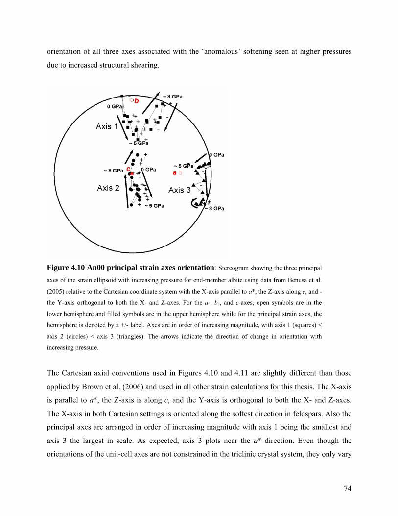
orientation of all three axes associated with the ‘anomalous’ softening seen at higher pressures

due to increased structural shearing.

Figure 4.10 An00 principal strain axes orientation: Stereogram showing the three principal

axes of the strain ellipsoid with increasing pressure for end-member albite using data from Benusa et al.

(2005) relative to the Cartesian coordinate system with the X-axis parallel to a*, the Z-axis along c, and -

the Y-axis orthogonal to both the X- and Z-axes. For the a-, b-, and c-axes, open symbols are in the

lower hemisphere and filled symbols are in the upper hemisphere while for the principal strain axes, the

hemisphere is denoted by a +/- label. Axes are in order of increasing magnitude, with axis 1 (squares) <

axis 2 (circles) < axis 3 (triangles). The arrows indicate the direction of change in orientation with

increasing pressure.

The Cartesian axial conventions used in Figures 4.10 and 4.11 are slightly different than those

applied by Brown et al. (2006) and used in all other strain calculations for this thesis. The X-axis

is parallel to a*, the Z-axis is along c, and the Y-axis is orthogonal to both the X- and Z-axes.

The X-axis in both Cartesian settings is oriented along the softest direction in feldspars. Also the

principal axes are arranged in order of increasing magnitude with axis 1 being the smallest and

axis 3 the largest in scale. As expected, axis 3 plots near the a* direction. Even though the

orientations of the unit-cell axes are not constrained in the triclinic crystal system, they only vary

74

within a couple of degrees with pressure and within 5 degrees with across all compositions. Also,

the large wander of both axis 1 and axis 2 at lower pressures, while the ‘tilting’ mechanism is in

effect, is most likely due to poorly constrained values from the almost circular shape of the strain

ellipse in the (100) plane below 5 GPa.

Figure 4.11 Plagioclase principal strain orientation: Stereogram showing the three principal axes of

the strain ellipsoid with increasing pressure for end-member albite (black), An20 (red), An68 (green) and An89

(magenta). The Cartesian coordinate system is the same as in Figure 4.10. For the principal strain axes, the

hemisphere is denoted by +/- labels. Axes are in order of increasing magnitude, with axis 1 (squares) < axis 2

(circles) < axis 3 (triangles). The low pressure ends of the trends are marked by the arrows

Figure 4.11 illustrates the pattern of orientation of the principal strain ellipsoid axes with

increasing anorthite content. The abrupt change in orientation of all three axes associated with

the shearing mechanism and softening in albite at higher pressures is absent in all other

compositions. Instead there is just the same pattern observed in An20 and up similar to that of

albite below about 5 GPa. There is also a general trend to smaller variations with increasing

anorthite content which is consistent with the stiffening seen in the compliance tensor sums at

room pressure away from albite. Overall, a clockwise rotation pattern is evident from albite to

anorthite.

75

The compliance tensor sums for both An89 and An96 can be related back to the spontaneous

strain variations associated with the P-1 to I-1 phase transition. Figure 4.12 shows the same

evolution with pressure in all the compliance tensor sums, including a maximum, in each sum at

the pressure corresponding to the discontinuity in the spontaneous strain and the change in the

unit-cell parameters, for both compositions. This similarity in strain with pressure supports the

conclusion that it is the P-1 to I-1 transition responsible for the discontinuity in An89 as well as

An96. The much broader, maximum in the An89 compliance tensor sums, compared to those of

An96, is likely the result of smaller domain size and also probably has a significant effect on the

extrapolation of the high-pressure values in calculation of the spontaneous strain (i.e. limited

leverage due to the wide range of pressures influenced by the change in elasticity).

76

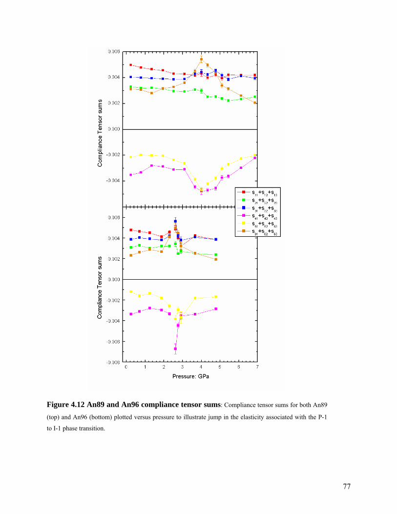
Figure 4.12 An89 and An96 compliance tensor sums: Compliance tensor sums for both An89

(top) and An96 (bottom) plotted versus pressure to illustrate jump in the elasticity associated with the P-1

to I-1 phase transition.

77

In addition, a linear or quadratic fit to the variation in the compliance tensor sums with pressure

for each individual composition was used to derive values of the compliance tensor sums at zero

pressure. These values for end-member albite were used by Brown et al. (2006) as constraints on

the inversion of ISLS (impulse stimulated light scattering) data for the same sample to yield

significantly reduced uncertainties on the derived full independent compliance tensor

components over what would be determined without the added constraints. They observed that

the values of the purely compressional components (C11, C22, and C33) supported the

observations of Benusa et al. (2005) as to the dominant structural mechanisms operating to

account for the trends seen in the unit-cell parameters, where C11, C22, and C33 correlate to the X,

Y and Z Cartesian axes respectively. That is, C11 had a much smaller or softer value than either

C22 or C33 consistent with the rotational mechanism closing the [100] crankshafts over the stiffer

flattening and shearing mechanisms of the four-membered rings corresponding to C22 and C33.

The determination of the full compliance tensor by Brown et al. (2006) is the first of its kind

published for feldspars not averaged to monoclinic symmetry, and one of only three for any

triclinic material.

Figure 4.13 Zero-pressure compliance tensor sums vs. composition: Compliance tensor

sums versus percent anorthite composition at P = 0 for both compressional terms (left) and shear terms

(right) with noted breaks in overall trends at the compositions corresponding to phase transitions from C-1

to I-1 (around An50) and I-1 to P-1 (around An90). There is also a decrease in the anisotropy of the

compressional terms as the Ca content is increased.

78

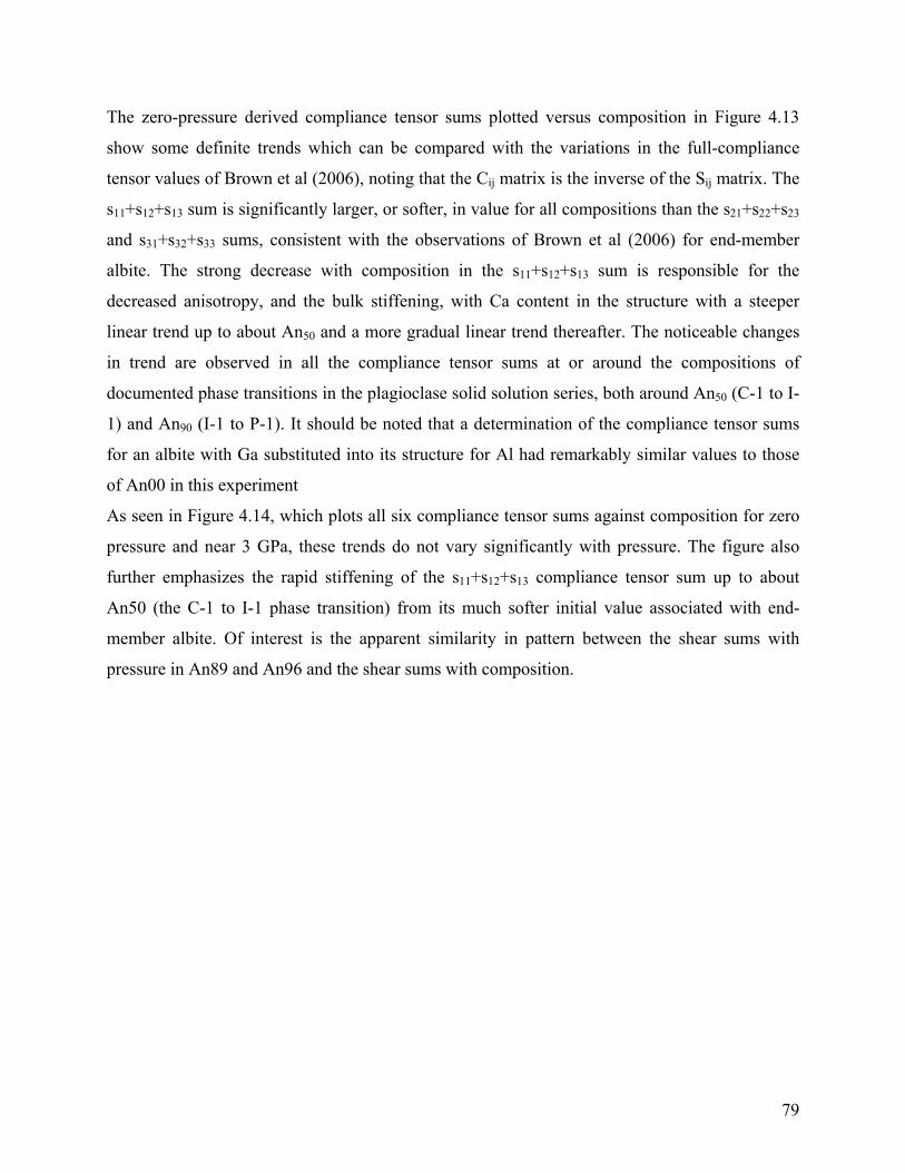
The zero-pressure derived compliance tensor sums plotted versus composition in Figure 4.13

show some definite trends which can be compared with the variations in the full-compliance

tensor values of Brown et al (2006), noting that the Cij matrix is the inverse of the Sij matrix. The

s11+s12+s13 sum is significantly larger, or softer, in value for all compositions than the s21+s22+s23

and s31+s32+s33 sums, consistent with the observations of Brown et al (2006) for end-member

albite. The strong decrease with composition in the s11+s12+s13 sum is responsible for the

decreased anisotropy, and the bulk stiffening, with Ca content in the structure with a steeper

linear trend up to about An50 and a more gradual linear trend thereafter. The noticeable changes

in trend are observed in all the compliance tensor sums at or around the compositions of

documented phase transitions in the plagioclase solid solution series, both around An50 (C-1 to I-

1) and An90 (I-1 to P-1). It should be noted that a determination of the compliance tensor sums

for an albite with Ga substituted into its structure for Al had remarkably similar values to those

of An00 in this experiment

As seen in Figure 4.14, which plots all six compliance tensor sums against composition for zero

pressure and near 3 GPa, these trends do not vary significantly with pressure. The figure also

further emphasizes the rapid stiffening of the s11+s12+s13 compliance tensor sum up to about

An50 (the C-1 to I-1 phase transition) from its much softer initial value associated with end-

member albite. Of interest is the apparent similarity in pattern between the shear sums with

pressure in An89 and An96 and the shear sums with composition.

79

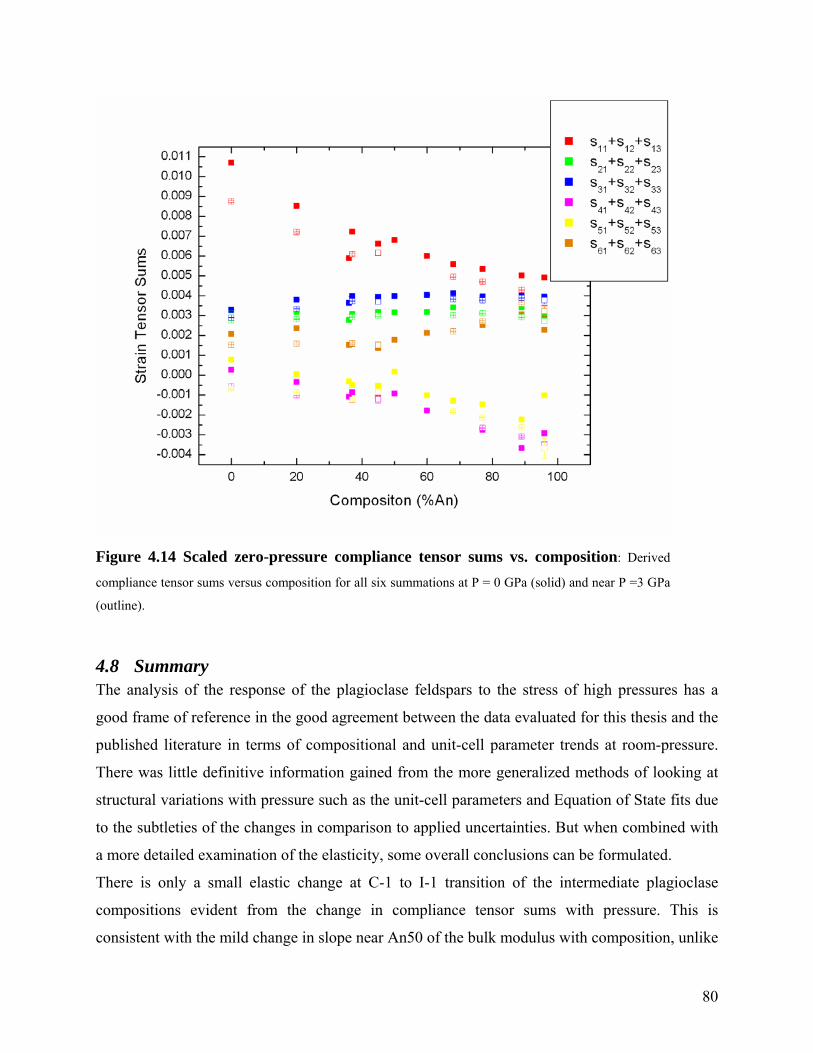
Figure 4.14 Scaled zero-pressure compliance tensor sums vs. composition: Derived

compliance tensor sums versus composition for all six summations at P = 0 GPa (solid) and near P =3 GPa

(outline).

4.8 Summary The analysis of the response of the plagioclase feldspars to the stress of high pressures has a

good frame of reference in the good agreement between the data evaluated for this thesis and the

published literature in terms of compositional and unit-cell parameter trends at room-pressure.

There was little definitive information gained from the more generalized methods of looking at

structural variations with pressure such as the unit-cell parameters and Equation of State fits due

to the subtleties of the changes in comparison to applied uncertainties. But when combined with

a more detailed examination of the elasticity, some overall conclusions can be formulated.

There is only a small elastic change at C-1 to I-1 transition of the intermediate plagioclase

compositions evident from the change in compliance tensor sums with pressure. This is

consistent with the mild change in slope near An50 of the bulk modulus with composition, unlike

80

the larger discontinuity that Angel (2004c) previously postulated. Also, the P-1 to I-1 transition

with pressure shows dominantly first-order behavior varying to more of a second-order nature

away from the anorthite end-member. The elastic response associated with this phase transition

seems to be of the same pattern as seen in the compliance tensor sum variation with composition

near anorthite, although no definitive correlation can be stated.

The comparison of the An37 structural changes with pressure with those of end-member albite

shows similar structural mechanisms operating between the two compositions. The evidence for

the closing of the [100] crankshafts is seen in albite up to about 6 GPa and in An37 through the

10 GPa hydrostatic limit. The secondary shearing mechanism responsible for the anomalous

softening in albite around 8 GPa is absent in the An37 data. Some hints are given that this

mechanism may operate at pressures in excess of 10 GPa, but no conclusive evidence for it were

seen in the present data.

The stiffening seen in elasticity change with pressure is consistent with structural changes seen

between An00 and An37. The minimal change in both the elasticity, with the substitution of Ga

into the framework, and the T-O bond distances, with pressure, points away from the tetrahedral

framework being a major contributor to the observed stiffening with increasing anorthite content.

The stiffening with composition is also not likely due to variations in degree of ordering between

samples. The changes in the nature of the extra-framework cation bonding scheme with the

substitution of Ca for Na is suspect as a possible explanation for the stiffening of the structure,

but not conclusively due to the uncertainty associated with the split site model used in the

structure refinements.

With feldspar as one of the most abundant elements in the Earth’s crust, the evaluation of its

physical properties is essential to geophysical, petrological, and materials applications. It is

important to develop a conceptual model to characterize plagioclase feldspar compression with

pressure for making any future extrapolations or interpolations. Though this thesis does not

identify the mechanistic model, it does recognize that the consistencies in the structural response

with pressure across the plagioclase solid solution series suggest common mechanisms.

81

References

Anderson OL (1995) Equations of state of solids for geophysics and ceramic science. Oxford

University Press, Oxford

Angel RJ (1988) High pressure structure of anorthite. Am Min 73:1114-1119

Angel RJ (1993) The high-pressure, high-temperature equation of state of calcium-fluoride,

CaF2. J Phys Cond Matter 5:L141-L144

Angel RJ (1994) Feldspars at high pressure. In Parsons I (ed.) Feldspars and their reactions. 271-

312

Angel RJ (2000) Equations of State. In Hazen RM, Downs RT (eds.) High-temperature and high-

pressure crystal chemistry. Rev Min Geochem 41:35-59

Angel RJ (2003) Automated profile analysis for single-crystal diffraction data. J Appl Cryst

36:295-300

Angel RJ (2004a) Absorption corrections for diamond-anvil pressure cells implemented in a

software package Absorb-6.0. J Appl Cryst 37:486-492

Angel RJ (2004b) Average-2.2 software. www.crystal.vt.edu/crystal/software

Angel RJ (2004c) Equations of state of plagioclase feldspar. Contrib Min Pet 146:506-512

Angel RJ, Allan DR, Miletich R, Finger LW (1997) The use of quartz as an internal pressure

standard in high-pressure crystallography. J Appl Cryst 30:461-466

Angel RJ, Bujak M, Zhao J, Gatta GD, Jacobsen SD (2007) Effective hydrostatic limits of

pressure media for high-pressure crystallographic studies. J Appl Cryst 40:26-32

Angel RJ, Carpenter MA, Finger LW (1990) Structural variation associated with compositional

variation and order-disorder behavior in anorthite-rich feldspars. Am Min 75:150-162

Angel RJ, Downs RT, Finger LW (2000) High-Temperature-High-Pressure Diffractometry. In

Hazen RM, Downs RT (eds.) High-temperature and high-pressure crystal chemistry. Rev

Min Geochem 41:559-596

Angel RJ, Redfern SAT, Ross NL (1989) Spontaneous strain below the I-1 – P-1 transition in

anorthite at pressure. Phys Chem Min 16:539-544

82

Benusa MD, Angel RJ, Ross NL (2005) Compression of albite, NaAlSi3O8. Am Min 90:1115-

1120

Birch F (1947) Finite elastic strain of cubic crystals. Phys Rev 71:809-824

Boffa-Ballaran T, Angel RJ, Carpenter MA (2000) High-pressure transformation behavior of the

cummingtonite-grunerite solid solution. Euro Journal of Min 12:1195-1213

Bown GE, Gay P (1958) The reciprocal lattice geometry of the plagioclase feldspar structures. Z

Krist 111:1-14

Bridgman PW (1928) The linear compressibility of thirteen natural crystals. Am Journal Sci

15:287-296

Brown JM, Abramson EH, Angel RJ (2006) Triclinic elastic constants for low albite. Phys Chem

Min 33:256-265

Brown WL, Openshaw RE, McMillan PC, Henderson CMB (1984) A review of the expansion

behavior of alkali feldspars: coupled variations in cell parameter and possible phase

transitions. Am Min 69:1058-1071

Burnham CW (1966) Computation of absorption corrections and the significance of end effects.

Am Min 51:159-167

Busing WR, Levy HA (1967) Angle calculations for 3- and 4-circle X-ray and neutron

diffractometers. Acta Cryst 22:457-464

Carpenter MA (1986) Experimental delineation of the "e" I1 and "e" C1 transformations in

intermediate plagioclase feldspars. Phys Chem Min 13:119-139

Carpenter MA (1992) Thermodynamics of phase transitions in minerals: a macroscopic approach

In Price GD, Ross NL (eds.) The Stability of Minerals, Min Soc GB, London: 173-215

Carpenter, MA (1994) Subsolidus phase relations of the plagioclase feldspar solid solution. In

Parsons I (ed) Feldspars and Their Reactions. Kluwer Academic Publishers, Netherlands:

221-269

Carpenter MA, McConnell JDC, Navrotsky A (1985) Enthalpies of ordering in the plagioclase

feldspar solid solution. Contrib Min Pet 87:138-148

Carpenter MA, Salje EKH, Graeme-Barber A (1998) Spontaneous strain as a determinant of

thermodynamic properties for phase transitions in minerals. Eur Journal Min 10:621-691

Clegg W, Blake AJ, Gould RO, Main P (2004) Crystal structure analysis- principles and practice.

Oxford University Press

83

Downs RT, Hazen RM, Finger LW (1994) The high-pressure crystal chemistry of low albite and

the origin of the pressure dependency of Al-Si ordering. Am Min 79:1042-1052

Downs RT, Yang HX, Hazen RM, Finger LW, Prewitt CT (1999) Compressibility mechanism of

alkali feldspars: new data from reedmergnerite. Am Min 84:333-340

Farrugia LJ (1999) WinGX suite for small-molecule single-crystal crystallography. J App Crys

32:837-838

Ferguson RB, Traill RJ, Taylor WH (1958) The crystal structures of low-temperature and high-

temperature albites. Acta Cryst 11:331-348

Finger LW, King HE (1978) A revised method of operation of the single-crystal diamond cell

and refinement of the structure of NaCl at 32 kbar. Am Min 63:337-342

Fleet SG, Chandrasekhar S, Megaw HD (1966) The structure of bytownite (‘body-centered

anorthite’). Acta Cryst 21:782-801

Forman RA, Piermarini GJ, Barnett JD, Block S (1972) Pressure measurement by utilization of

ruby sharp-line luminescence. Science 176:284-285

Gay P (1953) The structure of the plagioclase feldspars III: an X-ray study of anorthites and

bytownites. Min Mag 30:169-177

Gay P (1956) The structure of the plagioclase feldspars VI: natural intermediate plagioclases.

Min Mag 31:21-40

Grundy HD, Brown WL (1974) A high-temperature X-ray study of low and high plagioclase

feldspars. In WS, Zussman J (eds.) The Feldspars, Manchester Univ Press, Manchester,

UK: 162-173

Hamilton WC (1974) Angle settings for four-circle diffractometers. International Tables for X-

ray Crystallography 4:273-284

Harlow GE, Brown GE (1980) Low albite: an X-ray and neutron diffraction study Am Min

65:665-675

Hazen RM (1976) Sanidine: predicted and observed monoclinic-to-albite reversible

transformations at high pressure. Science 194:105-107

Hazen RM, Finger LW (1981) Calcium fluoride as an internal pressure standard in high-pressure

and temperature crystallography. J Appl Cryst 14:234-236

84

Hazen RM, Prewitt CT (1977) Linear compressiblities of low albite: high-pressure structural

implications. Am Min 62:554-558

King HE, Finger LW (1979) Diffracted beam crystal centering and its application to high-

pressure crystallography. J Appl Cryst 12:374-378

Kirkpatrick RJ, Kinsey RA, Smith KA, Henderson DM, Oldfield E (1985) High resolution solid-

state sodium-23, aluminium-27, and silicon-29 nuclear magnetic resonance spectroscopic

reconnaissance of alkali and plagioclase feldspar. Am Min 70:106-123

Kracek FC, Neuvonen KJ (1952) Thermochemistry of plagioclase and alkali feldspars. Am

Journal of Sci. Bowen Vol 293-318

Kroll H (1971) Determination of Al, Si distribution in alkali feldspars from X-ray powder data.

Neues Jahrb. Mineral. Monatschr. 2:91-94

Kroll H, Ribbe PH (1983) Lattice parameter, composition and Al/Si ordering in alkali feldspars

In Ribbe PH (ed) Reviews in Mineralogy Vol. 2 Feldspars, Min Soc Am: 57-99

Loewenstein W (1954) The distribution of aluminum in the tetrahedral of silicates and

aluminates. Am. Min. 39: 92-96

McLaren AC (1974) Transmission electron microscopy of the feldspars. In WS, Zussman J (eds.)

The Feldspars, Manchester Univ Press, Manchester, UK: 378-423

McLaren AC, Marshall DB (1974) Transmission electron microscope study of the domain

structures associated with the b-, c-, d-, e-, and f-reflections in plagioclase feldspars.

Contr Min Pet 44:237-249

McSkimmin HJ, Andreatch P, Thurston RM (1965) Elastic moduli of quartz versus hydrostatic

pressure at 25° and -195.8°C. J Appl Phys 36:1624-1633

Megaw, HD (1954) Notation for feldspar structures. Acta Crystallogr. 9: 56-60

Megaw, HD (1974) The architecture of the feldspars. In MacKenzie WS, Zussman J (eds.) The

Feldspars, Manchester Univ Press, Manchester, UK: 1-23

Miletich R (2000) The ETH diamond anvil cell Users Manual. Laboratory for Crystallography

ETH Zurich, Switzerland

Miletich R, Allen DR, Kuhs WF (2000) High-pressure single-crystal techniques. In Hazen RM,

Downs RT (eds.) High-temperature and high-pressure crystal chemistry. Rev Min

Geochem 41:445-519

85

Miletich R, Hejny C, Krauss G, Ullrich A (2005) Diffraction techniques: shedding light on

structural changes at extreme conditions. EMU Notes on Mineralogy 7:281-338

Miletich R, Reifler H, Kunz M (1999) The “ETH diamond-anvil cell” design for single-crystal

XRD at non-ambient conditions. Acta Cryst A55:99-100

Murnaghan FD (1937) Finite deformations of an elastic solid. Am Journal Math 49:235-260

Nwe YY (1976) Electron-probe studies of the earlier pyroxenes and olivines from the

Skaergaard intrusion, East Greenland. Contr Min Pet 55:105-126

Nye JF (1957) Physical Properties of Crystals. Oxford University Press, Oxford

Pavese A, Artioli G (1996) Profile-fitting treatment of single-crystal diffraction data. Acta Cryst

A52:890-897

Poirier J-P, Tarantola A (1998) A logarithmic equation of state. Phys Earth Planet Int 109:1-8

Rainey CS, Wenk HR (1978) Intensity differences of subsidiary reflections in calcic plagioclase.

Am Min 63:124-131

Ralph RL, Finger LW (1982) A computer program for refinement of crystal orientation matrix

and lattice constants from diffractometer data with lattice symmetry constraints. J Appl

Cryst 15:1357-1360

Redfern SAT, Salje EKH (1987) Thermodynamics of plagioclase II: temperature evolution of the

spontaneous strain at the I-1 ↔ P-1 phase transition in anorthite. Phys Chem Min 14:189-

195

Ribbe, PH (1983) Chemistry, structure and nomenclature of feldspars. Rev Mineral 2, 2nd ed: 1-

19

Ribbe PH (1994) The crystal structures of the aluminum-silicate feldspars. In Feldspars and

Their Reactions, Parsons I, eds Kluwer Academic Publishers, Netherlands: 1-49

Ribbe PH, Megaw HD, Taylor WH (1969) The albite structures. Acta Cryst B25:1503-1518

Salje EKH (1991) Crystallography and structural phase transitions, an introduction. Acta Cryst

A47:453-469

Salje EKH (1993) Phase transitions in ferroelectric and co-elastic crystals. Cambridge University

Press, Cambridge

86

Schlenker JL, Gibbs GV, Boisen MB (1978) Strain-tensor components expressed in terms of

lattice parameters. Acta Cryst A34:52-54

Smith JV (1974) Feldspar Minerals I: crystal structure and physical properties. Springer-Verlag.

Smith JV, Brown WL (1988) Feldspar Minerals I: crystal structures, physical, chemical, and

microtextural properties. Ch. 9

Stacey F, Brennan B, Irvine RD (1981) Finite strain theories and comparisons with seismological

data. Geophysical Surveys 4:189-232

Stewart DB, Ribbe PH (1983) Optical properties of feldspars. In Ribbe PH (ed) Reviews in

Mineralogy Vol. 2 Feldspars, Min Soc Am: 121-140

Stewart DB, Walker GW, Wright TL, Fahey JJ (1966) Physical properties of calcic labradorite

from Lake County, Oregon. Am Min 51:177-197

Subramaniam AP (1956) Mineralogy and petrology of the Sittampundi Complex, Salem District,

Madras State, India. Bulletin Geol Soc Am 67:317-390

Tagai T, Korekawa M (1981) Crystallographic investigation of the Huttenlocher exsolution at

high temperature. Phys Chem Min 7:77-81

Taylor, WH (1933) The structure of sanidine and other feldspars. Z. Kristallogr. 85:425-442

Vinet P, Ferrante J, Rose JH, Smith JR (1987) Compressibility of solids. J Geophys Res

92:9319-9325

Wenk HR, Joswig W, Tagai T, Korekawa M, Smith BK (1980) The average structure of An62-

66 labradorite. Am Min 65:81-95

Wenk HR, Nakajima Y (1980) Structure, formation and decomposition of APB’s in calcic

plagioclase. Phys Chem Min 6:169-186

Wright TL, Stewart DB (1968) X-ray and optical study of alkali feldspars: I. Determination of

composition and structural state from refined unit-cell parameters and 2V. Am Min

53:28-87

Xu JA, Mao HK, Hemley RJ, Jines E (2002) The moissanite anvil cell: a new tool for high-

pressure research. J Phys Cond Matter 14:11543-11548

87

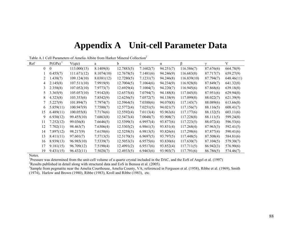
Appendix A Unit-cell Parameter Data Table A.1 Cell Parameters of Amelia Albite from Harker Mineral Collection2

Ref P(GPa) 1 V(qtz) a b c α β γ V0 0 113.000(15) 8.1409(8) 12.7883(5) 7.1602(7) 94.251(7) 116.586(7) 87.676(6) 664.78(9)1

0.455(7) 111.671(12) 8.1074(10) 12.7678(5) 7.1481(6) 94.246(9) 116.683(8) 87.717(7) 659.27(9)2 1.438(7) 109.124(10) 8.0381(12)

12.7280(5) 7.1231(7) 94.246(8) 116.839(10)

87.794(7) 648.46(11)

4 2.145(8) 107.511(10) 7.9919(9) 12.7004(5) 7.1064(6) 94.234(9) 116.928(8) 87.849(7) 641.32(8)3 2.358(8) 107.052(10) 7.9773(7) 12.6929(4) 7.1004(7) 94.220(7) 116.945(6) 87.868(6) 639.18(8)5 3.365(9) 105.057(10)

7.9142(8) 12.6575(4) 7.0794(7) 94.188(8) 117.045(8) 87.951(6) 629.94(8)

8 4.323(8) 103.353(6) 7.8542(9) 12.6256(5) 7.0572(7) 94.138(9) 117.099(8) 88.022(7) 621.39(9)7 5.227(9) 101.894(7) 7.7974(7) 12.5964(5) 7.0388(6) 94.070(8) 117.143(7) 88.089(6) 613.66(8)6 5.859(11) 100.947(9) 7.7580(7) 12.5772(4) 7.0251(5) 94.021(7) 117.156(7) 88.116(5) 608.41(7)

15 6.489(11) 100.055(8) 7.7176(6) 12.5592(4) 7.0113(4) 93.963(6) 117.177(6) 88.132(5) 603.11(6)9 6.930(12) 99.455(10)

7.6863(8) 12.5473(4) 7.0048(7) 93.908(7) 117.228(8) 88.111(5) 599.24(8)

11 7.252(12) 99.036(8) 7.6646(5) 12.5399(3) 6.9957(4) 93.877(6) 117.223(5) 88.072(4) 596.53(6)12 7.702(11) 98.463(7) 7.6306(4) 12.5303(2) 6.9861(3) 93.831(4) 117.268(4) 87.963(3) 592.41(5)14 7.897(12) 98.217(9) 7.6150(6) 12.5258(3) 6.9813(5) 93.826(6) 117.298(6) 87.877(4) 590.41(6)13 8.411(11) 97.601(7) 7.5713(5) 12.5170(3) 6.9697(5) 93.797(5) 117.448(5) 87.508(4) 584.81(6)16 8.939(13) 96.985(10) 7.5339(7) 12.5053(3) 6.9575(6) 93.830(6) 117.630(7) 87.104(5) 579.30(7)17 9.181(15) 96.709(12) 7.5190(4) 12.4991(2) 6.9517(6) 93.852(4) 117.711(5) 86.942(3) 576.90(6)19 9.431(15) 96.432(11) 7.5028(7) 12.4933(5) 6.9463(6) 93.903(7) 117.791(6) 86.786(5) 574.46(7)

Notes. 1Pressure was determined from the unit-cell volume of a quartz crystal included in the DAC, and the EoS of Angel et al. (1997) 2Results published in detail along with structural data and EoS in Benusa et al. (2005). 3Sample from pegmatite near the Amelia Courthouse, Amelia County, VA; referenced in Ferguson et al. (1958), Ribbe et al. (1969), Smith (1974), Harlow and Brown (1980), Ribbe (1983), Kroll and Ribbe (1983), etc.

88

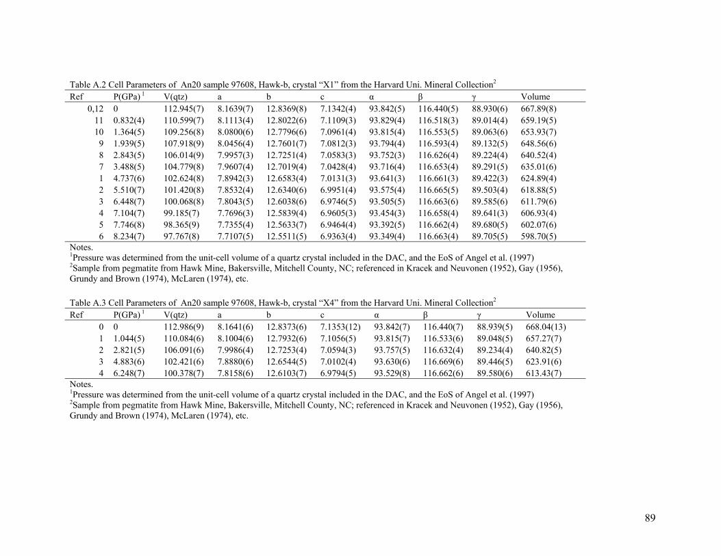
Table A.2 Cell Parameters of An20 sample 97608, Hawk-b, crystal “X1” from the Harvard Uni. Mineral Collection2

Ref P(GPa) 1 V(qtz) a b c α β γ Volume0,12 0 112.945(7) 8.1639(7) 12.8369(8) 7.1342(4) 93.842(5) 116.440(5) 88.930(6) 667.89(8)

11

0.832(4) 110.599(7) 8.1113(4) 12.8022(6) 7.1109(3) 93.829(4) 116.518(3) 89.014(4) 659.19(5)10 1.364(5) 109.256(8) 8.0800(6) 12.7796(6) 7.0961(4) 93.815(4) 116.553(5) 89.063(6) 653.93(7)

9 1.939(5) 107.918(9) 8.0456(4) 12.7601(7) 7.0812(3) 93.794(4) 116.593(4) 89.132(5) 648.56(6)8 2.843(5) 106.014(9) 7.9957(3) 12.7251(4) 7.0583(3) 93.752(3) 116.626(4) 89.224(4) 640.52(4)7 3.488(5) 104.779(8) 7.9607(4) 12.7019(4) 7.0428(4) 93.716(4) 116.653(4) 89.291(5) 635.01(6)1 4.737(6) 102.624(8) 7.8942(3) 12.6583(4) 7.0131(3) 93.641(3) 116.661(3) 89.422(3) 624.89(4)2 5.510(7) 101.420(8) 7.8532(4) 12.6340(6) 6.9951(4) 93.575(4) 116.665(5) 89.503(4) 618.88(5)3 6.448(7) 100.068(8)

7.8043(5) 12.6038(6) 6.9746(5) 93.505(5) 116.663(6) 89.585(6) 611.79(6)

4 7.104(7) 99.185(7) 7.7696(3) 12.5839(4) 6.9605(3) 93.454(3) 116.658(4) 89.641(3) 606.93(4)5 7.746(8) 98.365(9) 7.7355(4) 12.5633(7) 6.9464(4) 93.392(5) 116.662(4) 89.680(5) 602.07(6)6 8.234(7) 97.767(8) 7.7107(5) 12.5511(5) 6.9363(4) 93.349(4) 116.663(4) 89.705(5) 598.70(5)

Notes. 1Pressure was determined from the unit-cell volume of a quartz crystal included in the DAC, and the EoS of Angel et al. (1997) 2Sample from pegmatite from Hawk Mine, Bakersville, Mitchell County, NC; referenced in Kracek and Neuvonen (1952), Gay (1956), Grundy and Brown (1974), McLaren (1974), etc.

Table A.3 Cell Parameters of An20 sample 97608, Hawk-b, crystal “X4” from the Harvard Uni. Mineral Collection2

Ref P(GPa) 1 V(qtz) a b c α β γ Volume0 0 112.986(9) 8.1641(6) 12.8373(6) 7.1353(12) 93.842(7) 116.440(7) 88.939(5) 668.04(13)1

1.044(5) 110.084(6) 8.1004(6) 12.7932(6) 7.1056(5) 93.815(7) 116.533(6) 89.048(5) 657.27(7) 2 2.821(5) 106.091(6) 7.9986(4) 12.7253(4) 7.0594(3) 93.757(5) 116.632(4) 89.234(4) 640.82(5)3 4.883(6) 102.421(6) 7.8880(6) 12.6544(5) 7.0102(4) 93.630(6) 116.669(6) 89.446(5) 623.91(6)4 6.248(7) 100.378(7) 7.8158(6) 12.6103(7) 6.9794(5) 93.529(8) 116.662(6) 89.580(6) 613.43(7)

Notes. 1Pressure was determined from the unit-cell volume of a quartz crystal included in the DAC, and the EoS of Angel et al. (1997) 2Sample from pegmatite from Hawk Mine, Bakersville, Mitchell County, NC; referenced in Kracek and Neuvonen (1952), Gay (1956), Grundy and Brown (1974), McLaren (1974), etc.

89

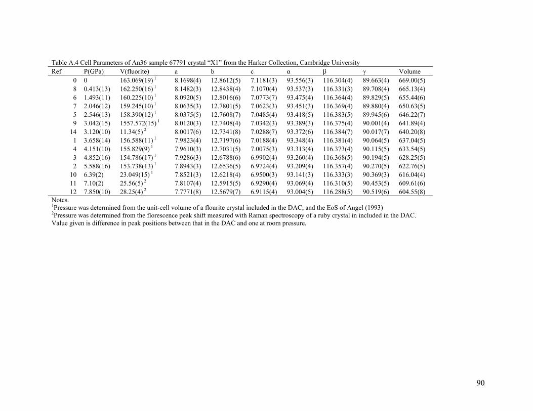
Table A.4 Cell Parameters of An36 sample 67791 crystal “X1” from the Harker Collection, Cambridge University

Ref P(GPa) V(fluorite) a b c α β γ Volume0 0 163.069(19) 1 8.1698(4) 12.8612(5) 7.1181(3) 93.556(3) 116.304(4) 89.663(4) 669.00(5)8

0.413(13) 162.250(16) 1 8.1482(3) 12.8438(4) 7.1070(4) 93.537(3) 116.331(3) 89.708(4) 665.13(4)6 1.493(11) 160.225(10) 1 8.0920(5) 12.8016(6) 7.0773(7) 93.475(4) 116.364(4) 89.829(5) 655.44(6)7 2.046(12) 159.245(10) 1 8.0635(3) 12.7801(5) 7.0623(3) 93.451(3) 116.369(4) 89.880(4) 650.63(5)5 2.546(13) 158.390(12) 1 8.0375(5) 12.7608(7) 7.0485(4) 93.418(5) 116.383(5) 89.945(6) 646.22(7)9 3.042(15) 1557.572(15) 1 8.0120(3) 12.7408(4) 7.0342(3) 93.389(3) 116.375(4) 90.001(4) 641.89(4)

14 3.120(10) 11.34(5) 2 8.0017(6) 12.7341(8) 7.0288(7) 93.372(6) 116.384(7) 90.017(7) 640.20(8)1 3.658(14) 156.588(11) 1 7.9823(4) 12.7197(6) 7.0188(4) 93.348(4) 116.381(4) 90.064(5) 637.04(5)4 4.151(10) 155.829(9) 1 7.9610(3) 12.7031(5) 7.0075(3) 93.313(4) 116.373(4) 90.115(5) 633.54(5)3 4.852(16) 154.786(17) 1 7.9286(3) 12.6788(6) 6.9902(4) 93.260(4) 116.368(5) 90.194(5) 628.25(5)2 5.588(16)

153.738(13) 1 7.8943(3) 12.6536(5) 6.9724(4) 93.209(4) 116.357(4) 90.270(5) 622.76(5)

10 6.39(2) 23.049(15) 1 7.8521(3) 12.6218(4) 6.9500(3) 93.141(3) 116.333(3) 90.369(3) 616.04(4)11 7.10(2) 25.56(5) 2 7.8107(4) 12.5915(5) 6.9290(4) 93.069(4) 116.310(5) 90.453(5) 609.61(6)12 7.850(10) 28.25(4) 2 7.7771(8) 12.5679(7) 6.9115(4) 93.004(5) 116.288(5) 90.519(6) 604.55(8)

Notes. 1Pressure was determined from the unit-cell volume of a flourite crystal included in the DAC, and the EoS of Angel (1993) 2Pressure was determined from the florescence peak shift measured with Raman spectroscopy of a ruby crystal in included in the DAC. Value given is difference in peak positions between that in the DAC and one at room pressure.

90

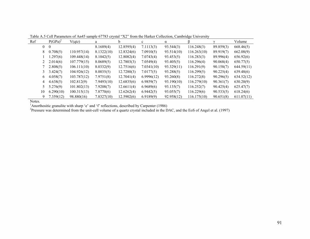
Table A.5 Cell Parameters of An45 sample 67783 crystal “X2” from the Harker Collection, Cambridge University

Ref P(GPa)2 V(qtz) a b c α β γ Volume0 0 8.1689(4) 12.8595(4) 7.1113(3) 93.544(3) 116.248(3) 89.859(3) 668.46(5)8

0.708(5) 110.957(14) 8.1322(10) 12.8324(6) 7.0910(5) 93.514(10) 116.263(10) 89.919(7) 662.08(9)1 1.297(6) 109.448(14) 8.1042(5) 12.8082(4) 7.0743(4) 93.453(5) 116.283(3) 89.996(4) 656.92(6)2 2.014(6) 107.779(15) 8.0689(5) 12.7803(3) 7.0549(4) 93.405(5) 116.296(4) 90.068(4) 650.77(5)7 2.808(5) 106.111(10) 8.0332(9) 12.7516(6) 7.0341(10) 93.329(11) 116.291(9) 90.158(7) 644.59(11)3 3.424(7) 104.926(12) 8.0035(5) 12.7280(3) 7.0177(5) 93.288(5) 116.299(5) 90.225(4) 639.48(6)6 4.058(7) 103.787(12)

7.9751(8) 12.7041(4) 6.9996(12)

93.260(8) 116.272(8) 90.296(5) 634.52(12)

4 4.638(5) 102.812(9) 7.9493(10) 12.6835(6) 6.9859(7) 93.190(10)

116.279(10)

90.361(7) 630.20(9)5 5.276(9) 101.802(13) 7.9208(7) 12.6611(4) 6.9689(6) 93.135(7) 116.252(7) 90.425(4) 625.47(7)

10 6.290(10) 100.315(13)

7.8770(6) 12.6262(4) 6.9442(5) 93.055(7) 116.229(6) 90.533(5) 618.24(6)9 7.359(12) 98.880(16) 7.8327(10) 12.5902(6) 6.9189(9) 92.958(12) 116.175(10) 90.651(8) 611.07(11)

Notes. 1Anorthositic granulite with sharp ‘e’ and ‘f’ reflections, described by Carpenter (1986) 2Pressure was determined from the unit-cell volume of a quartz crystal included in the DAC, and the EoS of Angel et al. (1997)

91

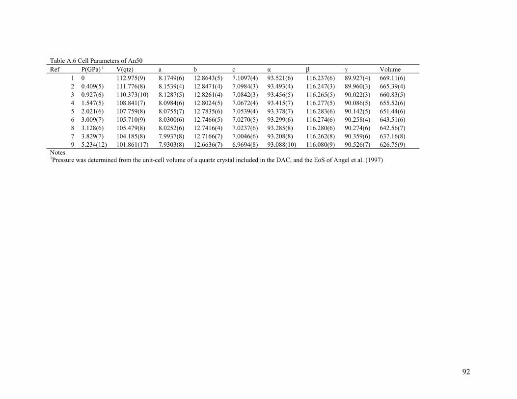
Table A.6 Cell Parameters of An50

Ref P(GPa) 1 V(qtz) a b c α β γ Volume1 0 112.975(9) 8.1749(6) 12.8643(5) 7.1097(4) 93.521(6) 116.237(6) 89.927(4) 669.11(6)2

0.409(5) 111.776(8) 8.1539(4) 12.8471(4) 7.0984(3) 93.493(4) 116.247(3) 89.960(3) 665.39(4)3 0.927(6) 110.373(10)

8.1287(5) 12.8261(4) 7.0842(3) 93.456(5) 116.265(5) 90.022(3) 660.83(5)

4 1.547(5) 108.841(7) 8.0984(6) 12.8024(5) 7.0672(4) 93.415(7) 116.277(5) 90.086(5) 655.52(6)5 2.021(6) 107.759(8) 8.0755(7) 12.7835(6) 7.0539(4) 93.378(7) 116.283(6) 90.142(5) 651.44(6)6 3.009(7) 105.710(9) 8.0300(6) 12.7466(5) 7.0270(5) 93.299(6) 116.274(6) 90.258(4) 643.51(6)8 3.128(6) 105.479(8) 8.0252(6) 12.7416(4) 7.0237(6) 93.285(8) 116.280(6) 90.274(6) 642.56(7)7 3.829(7) 104.185(8) 7.9937(8) 12.7166(7) 7.0046(6) 93.208(8) 116.262(8) 90.359(6) 637.16(8)9 5.234(12) 101.861(17) 7.9303(8) 12.6636(7) 6.9694(8) 93.088(10) 116.080(9) 90.526(7) 626.75(9)

Notes. 1Pressure was determined from the unit-cell volume of a quartz crystal included in the DAC, and the EoS of Angel et al. (1997)

92

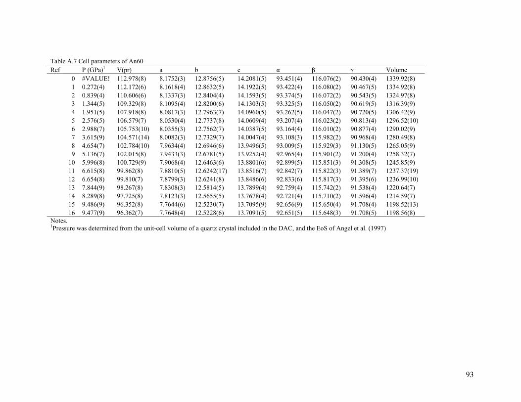
Table A.7 Cell parameters of An60

Ref P (GPa)1 V(pr) a b c α β γ Volume0 #VALUE! 112.978(8) 8.1752(3) 12.8756(5) 14.2081(5) 93.451(4) 116.076(2) 90.430(4) 1339.92(8)1

0.272(4) 112.172(6) 8.1618(4) 12.8632(5) 14.1922(5) 93.422(4) 116.080(2) 90.467(5) 1334.92(8)2 0.839(4) 110.606(6) 8.1337(3) 12.8404(4) 14.1593(5) 93.374(5) 116.072(2) 90.543(5) 1324.97(8)3 1.344(5) 109.329(8) 8.1095(4) 12.8200(6) 14.1303(5) 93.325(5) 116.050(2) 90.619(5) 1316.39(9)4 1.951(5) 107.918(8) 8.0817(3) 12.7963(7) 14.0960(5) 93.262(5) 116.047(2) 90.720(5) 1306.42(9)5 2.576(5) 106.579(7) 8.0530(4) 12.7737(8) 14.0609(4) 93.207(4) 116.023(2) 90.813(4) 1296.52(10)

6 2.988(7) 105.753(10) 8.0355(3) 12.7562(7) 14.0387(5) 93.164(4) 116.010(2) 90.877(4) 1290.02(9)7 3.615(9) 104.571(14) 8.0082(3) 12.7329(7) 14.0047(4) 93.108(3) 115.982(2) 90.968(4) 1280.49(8)8 4.654(7) 102.784(10)

7.9634(4) 12.6946(6) 13.9496(5) 93.009(5) 115.929(3) 91.130(5) 1265.05(9)

9 5.136(7) 102.015(8) 7.9433(3) 12.6781(5) 13.9252(4) 92.965(4) 115.901(2) 91.200(4) 1258.32(7)10 5.996(8) 100.729(9)

7.9068(4) 12.6463(6) 13.8801(6) 92.899(5) 115.851(3) 91.308(5) 1245.85(9)

11 6.615(8) 99.862(8) 7.8810(5) 12.6242(17)

13.8516(7) 92.842(7) 115.822(3) 91.389(7) 1237.37(19)12 6.654(8) 99.810(7) 7.8799(3) 12.6241(8) 13.8486(6) 92.833(6) 115.817(3) 91.395(6) 1236.99(10)

13 7.844(9) 98.267(8) 7.8308(3) 12.5814(5) 13.7899(4) 92.759(4) 115.742(2) 91.538(4) 1220.64(7)14 8.289(8) 97.725(8) 7.8123(3) 12.5655(5) 13.7678(4) 92.721(4) 115.710(2) 91.596(4) 1214.59(7)15 9.486(9) 96.352(8) 7.7644(6) 12.5230(7) 13.7095(9) 92.656(9) 115.650(4) 91.708(4) 1198.52(13)

16 9.477(9) 96.362(7) 7.7648(4) 12.5228(6) 13.7091(5) 92.651(5) 115.648(3) 91.708(5) 1198.56(8)Notes. 1Pressure was determined from the unit-cell volume of a quartz crystal included in the DAC, and the EoS of Angel et al. (1997)

93

Table A.8 Cell Parameters of An68 sample 115900, Lake County, from the P. Gay, U.S.N.M collection2

Ref P(GPa)1 V(flourite) a b c α β γ Volume5 0 163.061(13) 8.1742(3) 12.8722(7) 14.2022(6) 93.463(5) 116.068(3) 90.547(4) 1338.79(11)

13

1.240(9)

160.677(11)

8.1158(3) 12.8208(4) 14.1297(4) 93.305(4) 116.028(2) 90.760(5) 1317.70(8) 1 2.11(4) 159.14(5) 8.0757(4) 12.7860(9) 14.0778(9) 93.201(6) 115.991(3) 90.922(6) 1303.21(13)

11 2.905(11) 157.787(12) 8.0418(3) 12.7565(4) 14.0360(5) 93.105(4) 115.944(2) 91.057(4) 1291.45(8)14 3.430(9) 156.940(9) 8.0190(3) 12.7363(4) 14.0071(6) 93.052(5) 115.910(3) 91.142(4) 1283.46(8)

6 3.897(9) 156.210(8) 7.9988(3) 12.7190(5) 13.9817(5) 92.990(5) 115.880(2) 91.238(4) 1276.49(8)10 4.425(13) 155.409(16) 7.9771(2) 12.7004(3) 13.9538(5) 92.929(4) 115.844(2) 91.325(3) 1269.01(6)

7 4.727(13) 154.961(12) 7.9646(3) 12.6900(5) 13.9380(7) 92.908(6) 115.818(3) 91.367(5) 1264.82(9)8 5.277(13) 154.169(16) 7.9423(3) 12.6710(3) 13.9108(3) 92.834(3) 115.783(3) 91.465(5) 1257.31(6)9 5.630(12) 153.652(10) 7.9281(3) 12.6575(10) 13.8929(6) 92.797(6) 115.758(3) 91.514(5) 1252.38(12)

Notes. 1Pressure was determined from the unit-cell volume of a flourite crystal included in the DAC, and the EoS of Angel (1993) 2Sample from basalt phenocrysts in Lake County, Oregon; referenced in Stewart et al. (1966), McLaren and Marshall (1974), Rainey and Wenk (1978), Wenk and Nakajima (1980), Tagai and Korekawa (1981), etc.

94

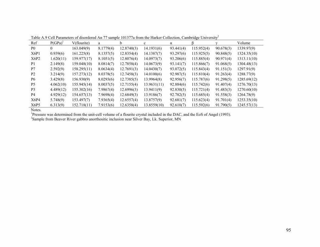
Table A.9 Cell Parameters of disordered An 77 sample 101377a from the Harker Collection, Cambridge University2

Ref P(GPa)1 V(flourite) a b c α β γ VolumeP0 0 163.049(9) 8.1779(4) 12.8740(3) 14.1931(6) 93.441(4) 115.952(4) 90.678(3) 1339.97(9)X6P1

0.939(6) 161.225(8) 8.1357(5) 12.8354(4) 14.1387(7) 93.297(6) 115.925(5) 90.848(5) 1324.35(10)X6P2

1.620(11)

159.977(17) 8.1051(5) 12.8076(4) 14.0973(7) 93.206(6) 115.885(4) 90.971(4) 1313.11(10)

P1 2.149(8) 159.048(10) 8.0814(7) 12.7858(4) 14.0673(9) 93.141(7) 115.866(7) 91.068(5) 1304.48(13) P7 2.592(9) 158.295(11) 8.0634(4) 12.7691(3) 14.0430(7) 93.072(5) 115.843(4) 91.151(3) 1297.91(9)

P2 3.214(9) 157.273(12)

8.0378(5) 12.7458(3) 14.0100(6) 92.987(5) 115.810(4) 91.263(4) 1288.77(9)P6 3.429(8) 156.930(9) 8.0293(6) 12.7385(5) 13.9964(8) 92.956(7) 115.787(6) 91.298(5) 1285.69(12)P5 4.062(10) 155.945(14) 8.0037(5) 12.7155(4) 13.9631(11)

92.884(6) 115.742(6) 91.407(4) 1276.70(13)

P3 4.489(12) 155.302(16) 7.9867(4) 12.6996(3) 13.9411(9) 92.830(5) 115.721(4) 91.483(3) 1270.60(10) P4 4.929(12)

154.657(13)

7.9698(4) 12.6849(3) 13.9186(7) 92.782(5) 115.685(4) 91.558(3) 1264.78(9)

X6P4 5.748(9) 153.497(7) 7.9365(4) 12.6557(4) 13.8757(9) 92.681(7) 115.623(4) 91.701(4) 1253.35(10)X6P5 6.313(9) 152.718(11) 7.9153(6) 12.6358(4) 13.8559(10) 92.610(7) 115.592(6) 91.790(5) 1245.57(13)Notes. 1Pressure was determined from the unit-cell volume of a flourite crystal included in the DAC, and the EoS of Angel (1993). 2Sample from Beaver River gabbro anorthositic inclusion near Silver Bay, Lk. Superior, MN

95

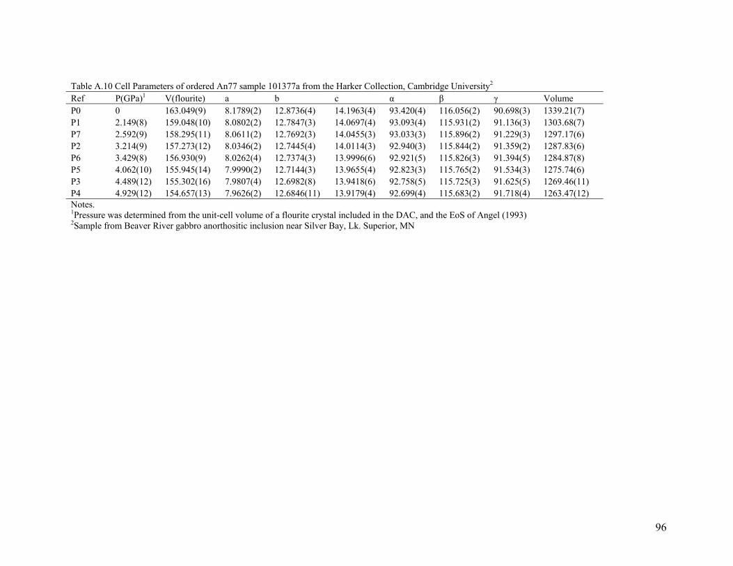
Table A.10 Cell Parameters of ordered An77 sample 101377a from the Harker Collection, Cambridge University2

Ref P(GPa)1 V(flourite) a b c α β γ VolumeP0 0 163.049(9) 8.1789(2) 12.8736(4) 14.1963(4) 93.420(4) 116.056(2) 90.698(3) 1339.21(7)P1

2.149(8) 159.048(10) 8.0802(2) 12.7847(3) 14.0697(4) 93.093(4) 115.931(2) 91.136(3) 1303.68(7)P7 2.592(9) 158.295(11) 8.0611(2) 12.7692(3) 14.0455(3) 93.033(3) 115.896(2) 91.229(3) 1297.17(6)P2 3.214(9) 157.273(12)

8.0346(2) 12.7445(4) 14.0114(3) 92.940(3) 115.844(2) 91.359(2) 1287.83(6)

P6 3.429(8) 156.930(9) 8.0262(4) 12.7374(3) 13.9996(6) 92.921(5) 115.826(3) 91.394(5) 1284.87(8)P5 4.062(10) 155.945(14) 7.9990(2) 12.7144(3) 13.9655(4) 92.823(3) 115.765(2) 91.534(3) 1275.74(6)P3 4.489(12) 155.302(16) 7.9807(4) 12.6982(8) 13.9418(6) 92.758(5) 115.725(3) 91.625(5) 1269.46(11)P4 4.929(12) 154.657(13) 7.9626(2) 12.6846(11) 13.9179(4) 92.699(4) 115.683(2) 91.718(4) 1263.47(12)Notes. 1Pressure was determined from the unit-cell volume of a flourite crystal included in the DAC, and the EoS of Angel (1993) 2Sample from Beaver River gabbro anorthositic inclusion near Silver Bay, Lk. Superior, MN

96

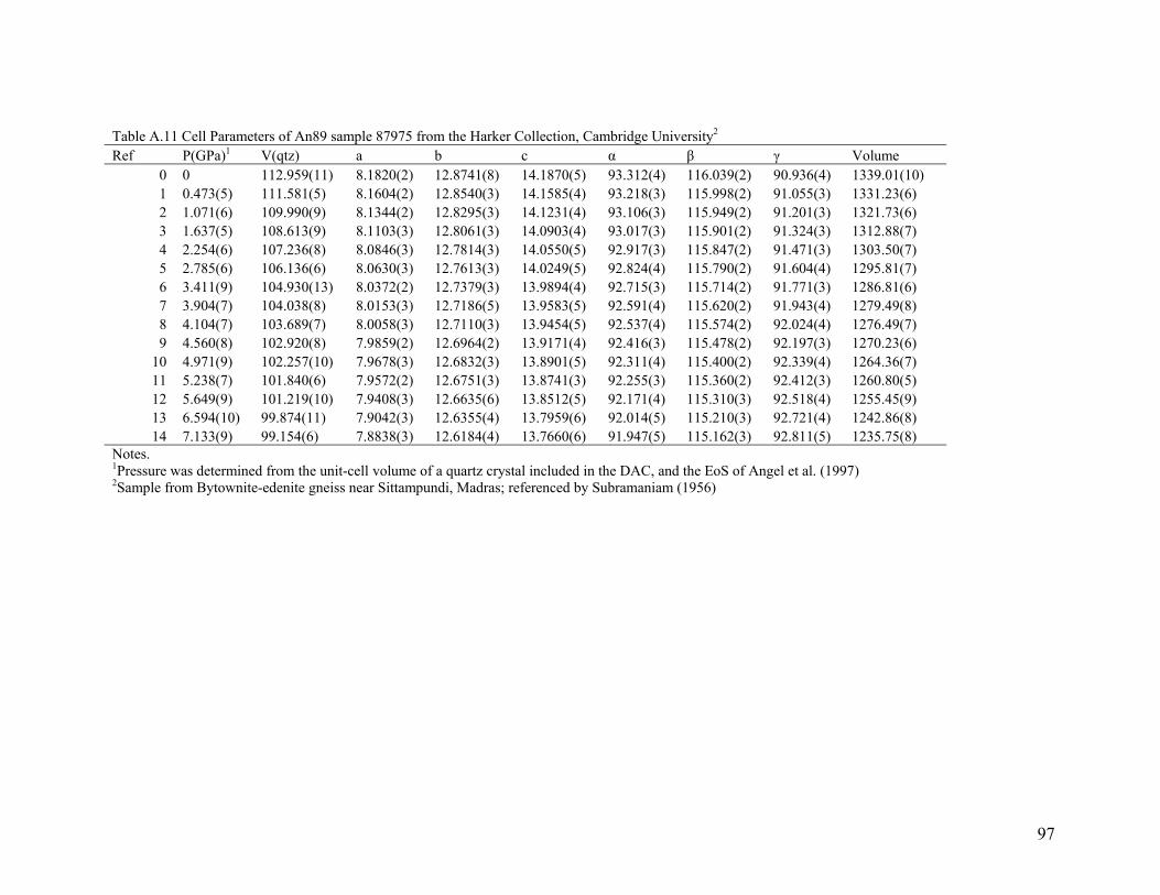
Table A.11 Cell Parameters of An89 sample 87975 from the Harker Collection, Cambridge University2

Ref P(GPa)1 V(qtz) a b c α β γ Volume0 0 112.959(11) 8.1820(2) 12.8741(8) 14.1870(5) 93.312(4) 116.039(2) 90.936(4) 1339.01(10)1

0.473(5) 111.581(5) 8.1604(2) 12.8540(3) 14.1585(4) 93.218(3) 115.998(2) 91.055(3) 1331.23(6) 2 1.071(6) 109.990(9) 8.1344(2) 12.8295(3) 14.1231(4) 93.106(3) 115.949(2) 91.201(3) 1321.73(6)3 1.637(5) 108.613(9) 8.1103(3) 12.8061(3) 14.0903(4) 93.017(3) 115.901(2) 91.324(3) 1312.88(7)4 2.254(6) 107.236(8) 8.0846(3) 12.7814(3) 14.0550(5) 92.917(3) 115.847(2) 91.471(3) 1303.50(7)5 2.785(6) 106.136(6) 8.0630(3) 12.7613(3) 14.0249(5) 92.824(4) 115.790(2) 91.604(4) 1295.81(7)6 3.411(9) 104.930(13)

8.0372(2) 12.7379(3) 13.9894(4) 92.715(3) 115.714(2) 91.771(3) 1286.81(6)

7 3.904(7) 104.038(8) 8.0153(3) 12.7186(5) 13.9583(5) 92.591(4) 115.620(2) 91.943(4) 1279.49(8)8 4.104(7) 103.689(7) 8.0058(3) 12.7110(3) 13.9454(5) 92.537(4) 115.574(2) 92.024(4) 1276.49(7)9 4.560(8) 102.920(8) 7.9859(2) 12.6964(2) 13.9171(4) 92.416(3) 115.478(2) 92.197(3) 1270.23(6)

10 4.971(9) 102.257(10)

7.9678(3) 12.6832(3) 13.8901(5) 92.311(4) 115.400(2) 92.339(4) 1264.36(7)11 5.238(7) 101.840(6) 7.9572(2) 12.6751(3) 13.8741(3) 92.255(3) 115.360(2) 92.412(3) 1260.80(5)12 5.649(9) 101.219(10)

7.9408(3) 12.6635(6) 13.8512(5) 92.171(4) 115.310(3) 92.518(4) 1255.45(9)

13 6.594(10)

99.874(11)

7.9042(3) 12.6355(4) 13.7959(6) 92.014(5) 115.210(3) 92.721(4) 1242.86(8)14 7.133(9) 99.154(6) 7.8838(3) 12.6184(4) 13.7660(6) 91.947(5) 115.162(3) 92.811(5) 1235.75(8)

Notes. 1Pressure was determined from the unit-cell volume of a quartz crystal included in the DAC, and the EoS of Angel et al. (1997) 2Sample from Bytownite-edenite gneiss near Sittampundi, Madras; referenced by Subramaniam (1956)

97

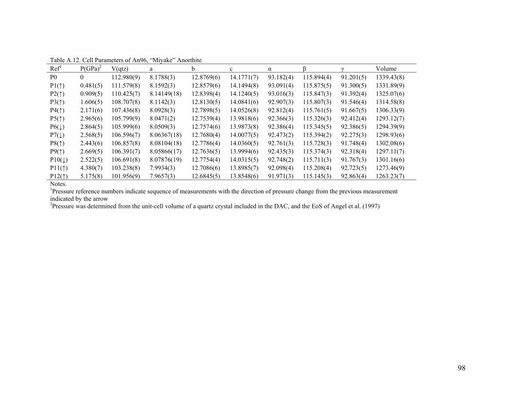
Table A.12. Cell Parameters of An96, “Miyake” Anorthite

Ref1 P(GPa)2 V(qtz) a b c α β γ VolumeP0 0 112.980(9) 8.1788(3) 12.8769(6) 14.1771(7) 93.182(4) 115.894(4) 91.201(5) 1339.43(8)P1(↑)

0.481(5) 111.579(8) 8.1592(3) 12.8579(6) 14.1494(8) 93.091(4) 115.875(5) 91.300(5) 1331.89(9)P2(↑) 0.909(5) 110.425(7) 8.14149(18)

12.8398(4) 14.1240(5) 93.016(3) 115.847(3) 91.392(4) 1325.07(6)

P3(↑) 1.606(5) 108.707(8) 8.1142(3) 12.8130(5) 14.0841(6) 92.907(3) 115.807(3) 91.546(4) 1314.58(8)P4(↑) 2.171(6) 107.436(8) 8.0928(3) 12.7898(5) 14.0526(8) 92.812(4) 115.761(5) 91.667(5) 1306.33(9)P5(↑) 2.965(6) 105.799(9) 8.0471(2) 12.7539(4) 13.9818(6) 92.366(3) 115.326(3) 92.412(4) 1293.12(7)P6(↓) 2.864(5) 105.999(6) 8.0509(3) 12.7574(6) 13.9873(8) 92.386(4) 115.345(5) 92.386(5) 1294.39(9)P7(↓) 2.568(5) 106.596(7) 8.06367(18) 12.7680(4) 14.0077(5) 92.473(2) 115.394(2) 92.275(3) 1298.93(6)P8(↑) 2.443(6) 106.857(8) 8.08104(18) 12.7786(4) 14.0360(5) 92.761(3) 115.728(3) 91.748(4) 1302.08(6)P9(↑) 2.669(5) 106.391(7) 8.05866(17) 12.7636(5) 13.9994(6) 92.435(3) 115.374(3) 92.318(4) 1297.11(7)P10(↓) 2.522(5) 106.691(8) 8.07876(19)

12.7754(4) 14.0315(5) 92.748(2) 115.711(3) 91.767(3) 1301.16(6)

P11(↑) 4.380(7) 103.238(8) 7.9934(3) 12.7086(6) 13.8985(7) 92.098(4) 115.208(4) 92.723(5) 1273.46(9)P12(↑) 5.175(8) 101.956(9) 7.9657(3) 12.6845(5) 13.8548(6) 91.971(3) 115.145(3) 92.863(4) 1263.23(7)Notes. 1Pressure reference numbers indicate sequence of measurements with the direction of pressure change from the previous measurement indicated by the arrow 2Pressure was determined from the unit-cell volume of a quartz crystal included in the DAC, and the EoS of Angel et al. (1997)

98

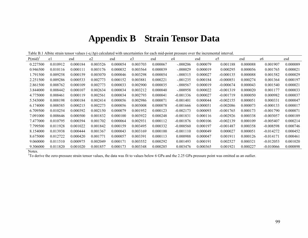
Appendix B Strain Tensor Data Table B.1 Albite strain tensor values (-ei/∆p) calculated with uncertainties for each mid-point pressure over the incremental interval. P(mid)1 e1 esd e2 esd e3 esd e4 esd e5 esd e6 esd0.227500 0.010912 0.000184 0.003526 0.000054 0.003703 0.000067 -.000206 0.000079 0.001188 0.000088 0.001907 0.0000890.946500

0.010116 0.000111 0.003176 0.000032 0.003564 0.000039 -.000029 0.000019 0.000295 0.000056 0.001765 0.0000211.791500 0.009258 0.000159 0.003070 0.000046 0.003298 0.000054 -.000315 0.000027 -0.000135 0.000088 0.001582 0.0000292.251500 0.009286 0.000533 0.002773 0.000152 0.003881 0.000221 -.001235 0.000184 -0.000851 0.000274 0.001364 0.0001972.861500 0.008762 0.000109 0.002773 0.000033 0.002900 0.000035 -.000567 0.000019 -0.000674 0.000043 0.001540 0.0000213.844000 0.008442 0.000107 0.002634 0.000034 0.003212 0.000040 -.000958 0.000022 -0.001319 0.000020 0.001177 0.0000334.775000 0.008461 0.000119 0.002561 0.000034 0.002793 0.000041 -0.001336 0.000027 -0.001719 0.000050 0.000982 0.0000375.543000 0.008198 0.000184 0.002414 0.000056 0.002986 0.000071 -0.001401 0.000044 -0.002155 0.000051 0.000331 0.0000476.174000 0.008585 0.000215 0.002273 0.000056 0.003008 0.000078 -0.001666 0.000051 -0.002086 0.000073 -0.000133 0.0000176.709500 0.010254 0.000392 0.002150 0.000079 0.001952 0.000123 -0.002173 0.000093 -0.001765 0.000173 -0.001790 0.0000717.091000 0.008646 0.000500 0.001832 0.000100 0.003922 0.000248 -0.001831 0.000116 -0.002926 0.000338 -0.003057 0.0001897.477000 0.010795 0.000394 0.001702 0.000064 0.002931 0.000112 -0.001876 0.000106 -0.002139 0.000109 -0.005407 0.0002147.799500 0.011928 0.001022 0.001842 0.000159 0.003495 0.000332 -0.000560 0.000197 -0.001487 0.000358 -0.008598 0.0007468.154000 0.013938 0.000444 0.001367 0.000043 0.003169 0.000100 -0.001110 0.000049 0.000027 0.000051 -0.014272 0.0004528.675000 0.012722 0.000420 0.001771 0.000057 0.003391 0.000113 0.000988 0.000047 0.001911 0.000126 -0.014171 0.0004619.060000 0.011510 0.000975 0.002049 0.000171 0.003552 0.000292 0.001493 0.000191 0.002527 0.000321 -0.012053 0.0010209.306000 0.011820 0.001020 0.001857 0.000173 0.003348 0.000285 0.003476 0.000365 0.001921 0.000227 -0.010066 0.000898

Notes. 1To derive the zero-pressure strain tensor values, the data was fit to values below 6 GPa and the 2.25 GPa pressure point was omitted as an outlier.

99

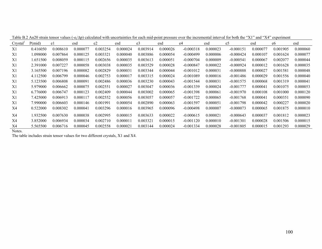
Table B.2 An20 strain tensor values (-ei/∆p) calculated with uncertainties for each mid-point pressure over the incremental interval for both the “X1” and “X4” experiment

Crystal1 P(mid) e1 esd e2 esd e3 esd e4 esd e5 esd e6 esd X1 0.416050 0.008610 0.000077 0.003254 0.000024 0.003914 0.000026 -0.000318 0.000023 -0.000151 0.000077 0.001905 0.000060X1

1.098000 0.007864 0.000125 0.003321 0.000040 0.003886 0.000054 -0.000499 0.000006 -0.000424 0.000107 0.001624 0.000077X1 1.651500 0.008059 0.000115 0.002656 0.000035 0.003613 0.000051 -0.000704 0.000009 -0.000541 0.000067 0.002077 0.000044X1 2.391000 0.007227 0.000058 0.003038 0.000035 0.003529 0.000028 -0.000847 0.000022 -0.000924 0.000012 0.001628 0.000035X1 3.165500 0.007196 0.000082 0.002829 0.000031 0.003344 0.000044 -0.001012 0.000031 -0.000888 0.000027 0.001581 0.000048X1 4.112500 0.006799 0.000046 0.002753 0.000017 0.003315 0.000024 -0.001089 0.000016 -0.001486 0.000029 0.001556 0.000040X1 5.123500 0.006808 0.000091 0.002486 0.000036 0.003230 0.000043 -0.001544 0.000031 -0.001575 0.000068 0.001319 0.000041X1 5.979000 0.006662 0.000075 0.002551 0.000027 0.003047 0.000036 -0.001339 0.000024 -0.001777 0.000041 0.001075 0.000053X1 6.776000 0.006747 0.000123 0.002409 0.000044 0.003002 0.000065 -0.001398 0.000061 -0.001970 0.000108 0.001000 0.000120X1 7.425000 0.006913 0.000117 0.002552 0.000056 0.003057 0.000057 -0.001722 0.000065 -0.001768 0.000041 0.000351 0.000090X1 7.990000 0.006603 0.000146 0.001991 0.000054 0.002890 0.000063 -0.001597 0.000051 -0.001798 0.000042 0.000227 0.000020X4 0.522000 0.008302 0.000041 0.003296 0.000016 0.003965 0.000096 -0.000498 0.000007 -0.000073 0.000065 0.001875 0.000010

X4 1.932500 0.007630 0.000038 0.002995 0.000015 0.003633 0.000022 -0.000615 0.000021 -0.000643 0.000037 0.001812 0.000023X4 3.852000 0.006934 0.000034 0.002710 0.000011 0.003321 0.000015 -0.001120 0.000010 -0.001301 0.000028 0.001506 0.000015X4 5.565500 0.006716 0.000045 0.002558 0.000021 0.003144 0.000024 -0.001334 0.000028 -0.001805 0.000015 0.001293 0.000029Notes. The table includes strain tensor values for two different crystals, X1 and X4.

100

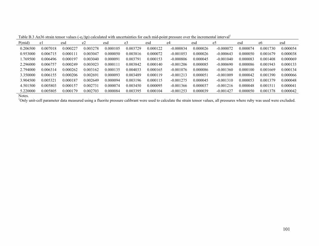
Table B.3 An36 strain tensor values (-ei/∆p) calculated with uncertainties for each mid-point pressure over the incremental interval1

P(mid) e1 esd e2 esd e3 esd e4 esd e5 esd e6 esd0.206500 0.007018 0.000227 0.003278 0.000105 0.003729 0.000122 -0.000834 0.000026 -0.000072 0.000074 0.001730 0.0000540.953000

0.006715 0.000111 0.003047 0.000050 0.003816 0.000072 -0.001053 0.000026 -0.000643 0.000050 0.001679 0.0000381.769500 0.006496 0.000197 0.003040 0.000091 0.003791 0.000153 -0.000806 0.000045 -0.001040 0.000083 0.001408 0.0000692.296000 0.006757 0.000249 0.003023 0.000111 0.003842 0.000140 -0.001206 0.000085 -0.000690 0.000086 0.001943 0.0001332.794000 0.006314 0.000262 0.003162 0.000135 0.004033 0.000165 -0.001076 0.000086 -0.001360 0.000100 0.001669 0.0001343.350000 0.006155 0.000206 0.002691 0.000093 0.003489 0.000119 -0.001213 0.000051 -0.001009 0.000042 0.001390 0.0000663.904500 0.005321 0.000187 0.002649 0.000094 0.003196 0.000115 -0.001275 0.000045 -0.001310 0.000053 0.001379 0.0000484.501500 0.005803 0.000157 0.002731 0.000074 0.003450 0.000095 -0.001366 0.000037 -0.001216 0.000048 0.001511 0.0000415.220000 0.005805 0.000179 0.002703 0.000084 0.003395 0.000104 -0.001253 0.000039 -0.001427 0.000050 0.001378 0.000042

Notes. 1Only unit-cell parameter data measured using a fluorite pressure calibrant were used to calculate the strain tensor values, all pressures where ruby was used were excluded.

101

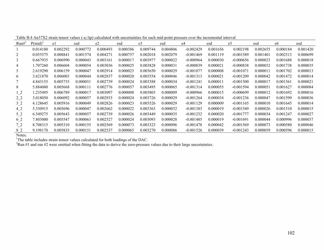
Table B.4 An37X2 strain tensor values (-ei/∆p) calculated with uncertainties for each mid-point pressure over the incremental interval

Run#1 P(mid)2 e1 esd e2 esd e3 esd e4 esd e5 esd e6 esd1 0.014180 0.002292 0.000772 0.000493 0.000386 0.009744 0.004806 -0.002429 0.001656 0.002198 0.002655 0.000184 0.0014202

0.055575 0.008841 0.001574 0.004271 0.000757 0.002018 0.002079 -0.001469 0.001119 -0.001589 0.001401 0.002513 0.0006993 0.667935 0.006990 0.000043 0.003161 0.000017 0.003977 0.000022 -0.000964 0.000030 -0.000656 0.000023 0.001688 0.0000184 1.707260 0.006604 0.000054 0.003036 0.000025 0.003828 0.000031 -0.000839 0.000021 -0.000838 0.000032 0.001738 0.0000355 2.619290 0.006159 0.000047 0.002914 0.000023 0.003650 0.000029 -0.001077 0.000008 -0.001071 0.000011 0.001702 0.0000136 3.621870 0.006003 0.000044 0.002837 0.000020 0.003554 0.000046 -0.001313 0.000021 -0.001209 0.000042 0.001472 0.0000147 4.843155 0.005755 0.000051 0.002739 0.000024 0.003388 0.000034 -0.001241 0.000011 -0.001500 0.000017 0.001561 0.0000218 5.884080 0.005668 0.000111 0.002776 0.000057 0.003495 0.000065 -0.001314 0.000055 -0.001594 0.000051 0.001627 0.0000841_2 1.235495 0.006789 0.000017 0.003097 0.000008 0.003803 0.000009 -0.000966 0.000015 -0.000699 0.000012 0.001692 0.0000162_2 3.018050 0.006092 0.000057 0.002933 0.000024 0.003726 0.000029 -0.001264 0.000034 -0.001236 0.000047 0.001599 0.0000363_2 4.128645 0.005916 0.000049 0.002826 0.000023 0.003526 0.000029 -0.001129 0.000009 -0.001165 0.000010 0.001645 0.0000144_2 5.330915 0.005696 0.000047 0.002662 0.000022 0.003363 0.000032 -0.001383 0.000019 -0.001549 0.000026 0.001510 0.0000155_2 6.549275 0.005643 0.000057 0.002739 0.000026 0.003449 0.000035 -0.001232 0.000020 -0.001777 0.000034 0.001247 0.0000276_2 7.803000 0.005547 0.000063 0.002527 0.000024 0.003093 0.000028 -0.001485 0.000019 -0.001691 0.000044 0.000996 0.0000377_2 8.708315 0.005310 0.000155 0.002569 0.000073 0.003323 0.000096 -0.001478 0.000042 -0.001569 0.000073 0.000580 0.0000468_2 9.198170 0.005835 0.000151 0.002537 0.000065 0.003270 0.000086 -0.001526 0.000039 -0.001243 0.000059 0.000596 0.000015Notes. 1The table includes strain tensor values calculated for both loadings of the DAC. 2Run #1 and run #2 were omitted when fitting the data to derive the zero-pressure values due to their large uncertainties.

102

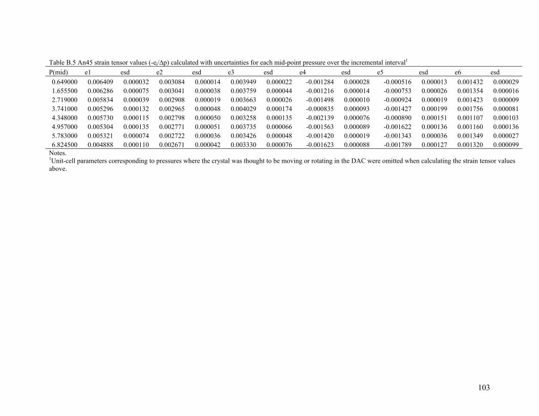
Table B.5 An45 strain tensor values (-ei/∆p) calculated with uncertainties for each mid-point pressure over the incremental interval1

P(mid) e1 esd e2 esd e3 esd e4 esd e5 esd e6 esd0.649000 0.006409 0.000032 0.003084 0.000014 0.003949 0.000022 -0.001284 0.000028 -0.000516 0.000013 0.001432 0.0000291.655500

0.006286 0.000075 0.003041 0.000038 0.003759 0.000044 -0.001216 0.000014 -0.000753 0.000026 0.001354 0.0000162.719000 0.005834 0.000039 0.002908 0.000019 0.003663 0.000026 -0.001498 0.000010 -0.000924 0.000019 0.001423 0.0000093.741000 0.005296 0.000132 0.002965 0.000048 0.004029 0.000174 -0.000835 0.000093 -0.001427 0.000199 0.001756 0.0000814.348000 0.005730 0.000115 0.002798 0.000050 0.003258 0.000135 -0.002139 0.000076 -0.000890 0.000151 0.001107 0.0001034.957000 0.005304 0.000135 0.002771 0.000051 0.003735 0.000066 -0.001563 0.000089 -0.001622 0.000136 0.001160 0.0001365.783000 0.005321 0.000074 0.002722 0.000036 0.003426 0.000048 -0.001420 0.000019 -0.001343 0.000036 0.001349 0.0000276.824500 0.004888 0.000110 0.002671 0.000042 0.003330 0.000076 -0.001623 0.000088 -0.001789 0.000127 0.001320 0.000099

Notes. 1Unit-cell parameters corresponding to pressures where the crystal was thought to be moving or rotating in the DAC were omitted when calculating the strain tensor values above.

103

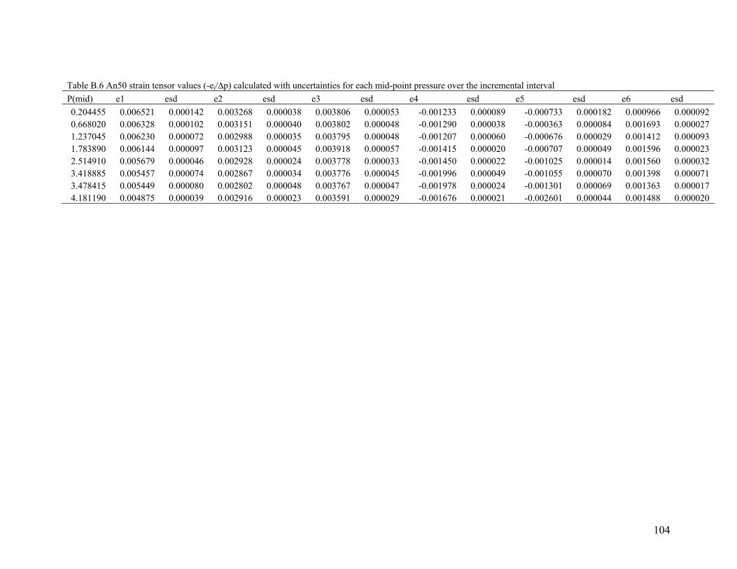
Table B.6 An50 strain tensor values (-ei/∆p) calculated with uncertainties for each mid-point pressure over the incremental interval

P(mid) e1 esd e2 esd e3 esd e4 esd e5 esd e6 esd0.204455 0.006521 0.000142 0.003268 0.000038 0.003806 0.000053 -0.001233 0.000089 -0.000733 0.000182 0.000966 0.0000920.668020

0.006328 0.000102 0.003151 0.000040 0.003802 0.000048 -0.001290 0.000038 -0.000363 0.000084 0.001693 0.0000271.237045 0.006230 0.000072 0.002988 0.000035 0.003795 0.000048 -0.001207 0.000060 -0.000676 0.000029 0.001412 0.0000931.783890 0.006144 0.000097 0.003123 0.000045 0.003918 0.000057 -0.001415 0.000020 -0.000707 0.000049 0.001596 0.0000232.514910 0.005679 0.000046 0.002928 0.000024 0.003778 0.000033 -0.001450 0.000022 -0.001025 0.000014 0.001560 0.0000323.418885 0.005457 0.000074 0.002867 0.000034 0.003776 0.000045 -0.001996 0.000049 -0.001055 0.000070 0.001398 0.0000713.478415 0.005449 0.000080 0.002802 0.000048 0.003767 0.000047 -0.001978 0.000024 -0.001301 0.000069 0.001363 0.0000174.181190 0.004875 0.000039 0.002916 0.000023 0.003591 0.000029 -0.001676 0.000021 -0.002601 0.000044 0.001488 0.000020

104

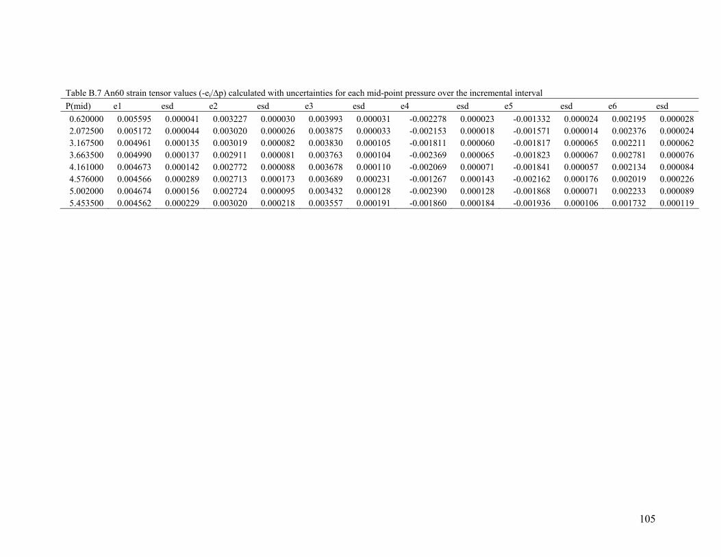
Table B.7 An60 strain tensor values (-ei/∆p) calculated with uncertainties for each mid-point pressure over the incremental interval P(mid) e1 esd e2 esd e3 esd e4 esd e5 esd e6 esd

0.620000 0.005595 0.000041 0.003227 0.000030 0.003993 0.000031 -0.002278 0.000023 -0.001332 0.000024 0.002195 0.0000282.072500

0.005172 0.000044 0.003020 0.000026 0.003875 0.000033 -0.002153 0.000018 -0.001571 0.000014 0.002376 0.0000243.167500 0.004961 0.000135 0.003019 0.000082 0.003830 0.000105 -0.001811 0.000060 -0.001817 0.000065 0.002211 0.0000623.663500 0.004990 0.000137 0.002911 0.000081 0.003763 0.000104 -0.002369 0.000065 -0.001823 0.000067 0.002781 0.0000764.161000 0.004673 0.000142 0.002772 0.000088 0.003678 0.000110 -0.002069 0.000071 -0.001841 0.000057 0.002134 0.0000844.576000 0.004566 0.000289 0.002713 0.000173 0.003689 0.000231 -0.001267 0.000143 -0.002162 0.000176 0.002019 0.0002265.002000 0.004674 0.000156 0.002724 0.000095 0.003432 0.000128 -0.002390 0.000128 -0.001868 0.000071 0.002233 0.0000895.453500 0.004562 0.000229 0.003020 0.000218 0.003557 0.000191 -0.001860 0.000184 -0.001936 0.000106 0.001732 0.000119

105

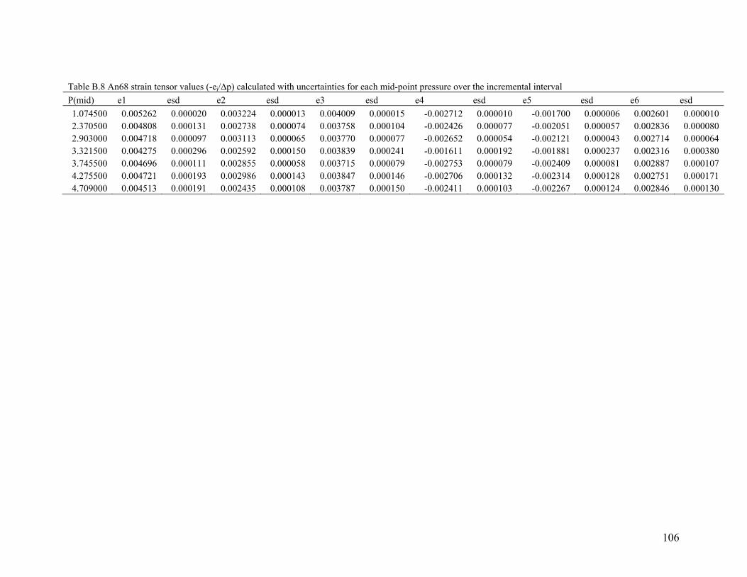
Table B.8 An68 strain tensor values (-ei/∆p) calculated with uncertainties for each mid-point pressure over the incremental interval

P(mid) e1 esd e2 esd e3 esd e4 esd e5 esd e6 esd1.074500 0.005262 0.000020 0.003224 0.000013 0.004009 0.000015 -0.002712 0.000010 -0.001700 0.000006 0.002601 0.0000102.370500

0.004808 0.000131 0.002738 0.000074 0.003758 0.000104 -0.002426 0.000077 -0.002051 0.000057 0.002836 0.0000802.903000 0.004718 0.000097 0.003113 0.000065 0.003770 0.000077 -0.002652 0.000054 -0.002121 0.000043 0.002714 0.0000643.321500 0.004275 0.000296 0.002592 0.000150 0.003839 0.000241 -0.001611 0.000192 -0.001881 0.000237 0.002316 0.0003803.745500 0.004696 0.000111 0.002855 0.000058 0.003715 0.000079 -0.002753 0.000079 -0.002409 0.000081 0.002887 0.0001074.275500 0.004721 0.000193 0.002986 0.000143 0.003847 0.000146 -0.002706 0.000132 -0.002314 0.000128 0.002751 0.0001714.709000 0.004513 0.000191 0.002435 0.000108 0.003787 0.000150 -0.002411 0.000103 -0.002267 0.000124 0.002846 0.000130

106

Table B.9 An77 (ordered) strain tensor values (-ei/∆p) calculated with uncertainties for each mid-point pressure over the incremental interval

P(mid)1 e1 esd e2 esd e3 esd e4 esd e5 esd e6 esd0.469500 0.005357 0.000043 0.003198 0.000022 0.003929 0.000027 -0.002730 0.000042 -0.001179 0.000035 0.002153 0.0000621.279500

0.005137 0.000096 0.003184 0.000059 0.004172 0.000077 -0.002397 0.000044 -0.001595 0.000041 0.002300 0.0000511.884500 0.005345 0.000169 0.003220 0.000083 0.003907 0.000104 -0.002190 0.000066 -0.001322 0.000144 0.002449 0.0000832.370500 0.004700 0.000195 0.002950 0.000082 0.003753 0.000108 -0.002771 0.000111 -0.001462 0.000190 0.002245 0.0001432.903000 0.004773 0.000100 0.002936 0.000060 0.003654 0.000076 -0.002430 0.000050 -0.001566 0.000036 0.002264 0.0000563.321500 0.004108 0.000272 0.002665 0.000166 0.004386 0.000257 -0.002613 0.000224 -0.002093 0.000267 0.001834 0.0002043.745500 0.004560 0.000095 0.002855 0.000059 0.003660 0.000082 -0.002032 0.000051 -0.001844 0.000048 0.002300 0.0000664.275500 0.004685 0.000186 0.002930 0.000109 0.003582 0.000136 -0.002246 0.000093 -0.001479 0.000130 0.002308 0.0001084.709000 0.004246 0.000164 0.002632 0.000102 0.003577 0.000142 -0.001955 0.000075 -0.001968 0.000078 0.002296 0.0000895.338500 0.004597 0.000084 0.002814 0.000052 0.003665 0.000070 -0.002199 0.000060 -0.001976 0.000039 0.002253 0.0000616.030500 0.004381 0.000125 0.002785 0.000063 0.002425 0.000056 -0.002181 0.000049 -0.002054 0.000102 0.001937 0.000057

Notes. 1The 3.32 GPa midpoint pressure values were excluded as outliers when fitting the strain tensor values to derive the zero-pressure compliance tensor sums.

107

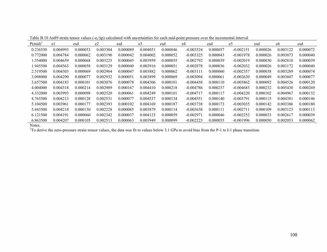
Table B.10 An89 strain tensor values (-ei/∆p) calculated with uncertainties for each mid-point pressure over the incremental interval

P(mid)1 e1 esd e2 esd e3 esd e4 esd e5 esd e6 esd0.236550 0.004993 0.000053 0.003304 0.000089 0.004051 0.000046 -0.003524 0.000057 -0.002151 0.000026 0.003122 0.0000720.772000

0.004784 0.000062 0.003190 0.000042 0.004002 0.000052 -0.003325 0.000043 -0.001978 0.000026 0.003073 0.0000401.354000 0.004659 0.000068 0.003225 0.000045 0.003959 0.000055 -0.002792 0.000039 -0.002019 0.000030 0.002810 0.0000391.945500 0.004563 0.000058 0.003129 0.000040 0.003916 0.000051 -0.002878 0.000036 -0.002032 0.000026 0.003172 0.0000402.519500 0.004303 0.000069 0.002964 0.000047 0.003882 0.000062 -0.003111 0.000060 -0.002357 0.000038 0.003289 0.0000743.098000 0.004290 0.000077 0.002932 0.000051 0.003899 0.000069 -0.003094 0.000061 -0.002630 0.000049 0.003607 0.0000773.657500 0.004183 0.000101 0.003076 0.000078 0.004306 0.000101 -0.004458 0.000110 -0.003862 0.000092 0.004526 0.0001204.004000 0.004318 0.000214 0.002989 0.000167 0.004410 0.000218 -0.004786 0.000237 -0.004683 0.000232 0.005430 0.0002694.332000 0.003993 0.000098 0.002520 0.000061 0.004249 0.000101 -0.004717 0.000117 -0.004220 0.000102 0.004967 0.0001324.765500 0.004213 0.000128 0.002531 0.000077 0.004537 0.000134 -0.004551 0.000140 -0.003791 0.000115 0.004381 0.0001465.104500 0.003961 0.000177 0.002393 0.000102 0.004169 0.000187 -0.003738 0.000173 -0.003035 0.000142 0.003386 0.0001805.443500 0.004218 0.000130 0.002228 0.000085 0.003879 0.000114 -0.003638 0.000111 -0.002711 0.000109 0.003123 0.0001136.121500 0.004191 0.000060 0.002342 0.000037 0.004123 0.000059 -0.002971 0.000046 -0.002252 0.000033 0.002617 0.0000396.863500 0.004207 0.000105 0.002513 0.000063 0.003949 0.000099 -0.002223 0.000055 -0.001996 0.000050 0.002053 0.000062

Notes. 1To derive the zero-pressure strain tensor values, the data was fit to values below 3.1 GPa to avoid bias from the P-1 to I-1 phase transition.

108

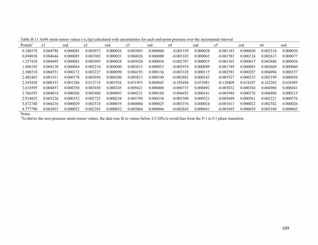
Table B.11 An96 strain tensor values (-ei/∆p) calculated with uncertainties for each mid-point pressure over the incremental interval P(mid)1 e1 esd e2 esd e3 esd e4 esd e5 esd e6 esd

0.240370 0.004786 0.000045 0.003072 0.000026 0.003883 0.000040 -0.003359 0.000028 -0.001183 0.000050 0.002316 0.0000200.694930

0.004644 0.000085 0.003305 0.000053 0.004026 0.000080 -0.003103 0.000062 -0.001583 0.000124 0.002613 0.0000771.257410 0.004495 0.000042 0.002995 0.000028 0.003920 0.000036 -0.002787 0.000025 -0.001365 0.000017 0.002886 0.0000261.888105 0.004120 0.000064 0.003210 0.000040 0.003813 0.000052 -0.002974 0.000049 -0.001789 0.000083 0.002669 0.0000602.306510 0.004551 0.000172 0.003227 0.000098 0.004193 0.000136 -0.003328 0.000115 -0.002583 0.000207 0.004094 0.0001572.482465 0.001911 0.000178 0.003056 0.000280 0.003813 0.000349 -0.002882 0.000343 -0.003527 0.000325 0.003199 0.0004562.545420 -0.008353 0.001286 0.012715 0.001926 0.031953 0.004842 -0.105494 0.015981 -0.120409 0.018247 0.162285 0.0245852.618595 0.004857 0.000350 0.003450 0.000245 0.005621 0.000400 -0.006715 0.000492 -0.003832 0.000364 0.004960 0.0004412.766555 0.004014 0.000206 0.002480 0.000095 0.004221 0.000169 -0.004455 0.000181 -0.002944 0.000276 0.004488 0.0002152.914825 0.003226 0.000352 0.002725 0.000238 0.003794 0.000338 -0.003508 0.000321 -0.003689 0.000561 0.003221 0.0003763.672740 0.004216 0.000029 0.002514 0.000019 0.004084 0.000025 -0.003376 0.000024 -0.001813 0.000022 0.002542 0.0000264.777790 0.003853 0.000052 0.002383 0.000032 0.003864 0.000046 -0.002845 0.000041 -0.001695 0.000039 0.001949 0.000043

Notes. 1To derive the zero-pressure strain tensor values, the data was fit to values below 2.5 GPa to avoid bias from the P-1 to I-1 phase transition.

109

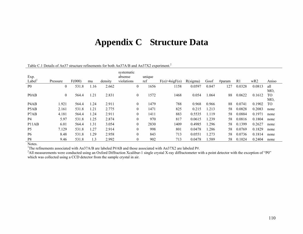
Appendix C Structure Data

Table C.1 Details of An37 structure refinements for both An37A/B and An37X2 experiment.2

Exp. Label1 Pressure F(000) mu density

systematic absense violations

unique ref F(o)>4sigF(o) R(sigma) Goof #param R1 wR2 Aniso

P0 0 531.8 1.16 2.662 0 1656 1158 0.0597 0.847 127 0.0328 0.0813 all

P0AB

0 564.4 1.21 2.831 0 1572 1468 0.054 1.064 88 0.0622 0.1612MO, TO

P4AB 1.921 564.4 1.24 2.911 0 1479 788 0.968 0.966 88 0.0741 0.1902 MO, TO

P5AB 2.161 531.8 1.21 2.775 0 1471 825 0.215 1.213 58 0.0828 0.2083 noneP7AB 4.181 564.4 1.24 2.911 0 1411 883 0.5535 1.119 58 0.0884 0.1971 noneP4 5.97 531.8 1.25 2.874 0 970 817 0.0615 1.239 58 0.0816 0.1804 noneP11AB 6.01 564.4 1.31 3.054 0 2830 1409 0.4985 1.296 58 0.1399 0.2627 noneP5 7.129 531.8 1.27 2.914 0 998 801 0.0478 1.286 58 0.0769 0.1829 noneP6 8.48 531.8 1.29 2.958 0 843 713 0.0551 1.273 58 0.0736 0.1814 noneP8 9.46 531.8 1.3 2.992 0 902 713 0.0478 1.589 58 0.1024 0.2404 noneNotes. 1The refinements associated with An37A/B are labeled P#AB and those associated with An37X2 are labeled P#. 2All measurements were conducted using an Oxford Diffraction Xcalibur-1 single crystal X-ray diffractometer with a point detector with the exception of “P0” which was collected using a CCD detector from the sample crystal in air.

110

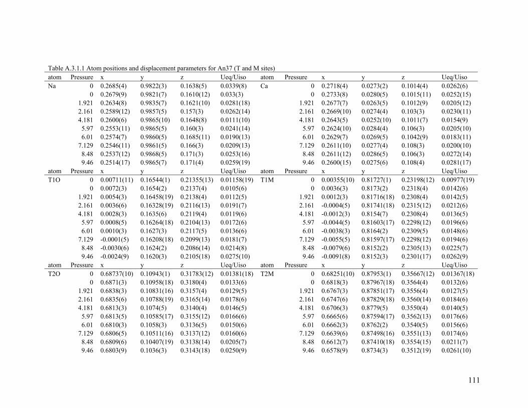
Table A.3.1.1 Atom positions and displacement parameters for An37 (T and M sites)

atom Pressure x y z Ueq/Uiso atom Pressure x y z Ueq/UisoNa 0 0.2685(4) 0.9822(3) 0.1638(5) 0.0339(8) Ca 0 0.2718(4) 0.0273(2) 0.1014(4) 0.0262(6) 0 0.2679(9) 8) 1.921 ) 0. ) 0. ) 0. 2) 1 0. 2) ) 0.0262(14) 2.161 0.2669(10) 0.0274(4) 0.103(3) 0.0230(11) 4.181 0.2600(6) 0.9865(10) 0.1648(8) 0.0111(10) 4.181 0.2643(5) 0.0252(10) 0.1011(7) 0.0154(9) 5.97 0.2553(11) 0.9865(5) 0.160(3) 0.0241(14) 5.97 0.2624(10) 0.0284(4) 0.106(3) 0.0205(10) 6.01 0.2574(7) 0.9860(5) 0.1685(11) 0.0190(13) 6.01 0.2629(7) 0.0269(5) 0.1042(9) 0.0183(11) 7.129 0.2546(11) 0.9861(5) 0.166(3) 0.0209(13) 7.129 0.2611(10) 0.0277(4) 0.108(3) 0.0200(10) 8.48 0.2537(12) 0.9868(5) 0.171(3) 0.0253(16) 8.48 0.2611(12) 0.0286(5) 0.106(3) 0.0272(14) 9.46 0.2514(17) 0.9865(7) 0.171(4) 0.0259(19) 9.46 0.2600(15) 0.0275(6) 0.108(4) 0.0281(17) atom Pressure x y z Ueq/Uiso atom Pressure x y z Ueq/Uiso T1O 0 0.00711(11) 0.16544(1) 0.21355(13) 0.01158(19) T1M 0 0.00355(10) 0.81727(1) 0.23198(12) 0.00977(19)

0.9821(7) 0.1610(12) 0.033(3)0.0281(1

0 0.2733(8)0.2677(7

0.0280(5)0263(5

0.1015(11)1012(9

0.0252(15)0205(11.921

2.16 0.2634(8)

2589(10.9835(7)0.9857(5

0.1621(10)0.157(3)

0 0.0072(3) 0.1654(2) 0.2137(4) 0.0105(6) 0 0.0036(3) 0.8173(2) 0.2318(4) 0.0142(6) 1.921 0.0054(3) 0.16458(19) 0.2138(4) 0.0112(5) 1.921 0.0012(3) 0.81716(18) 0.2308(4) 0.0142(5) 2.161 0.0036(6) 0.16328(19) 0.2116(13) 0.0191(7) 2.161 -0.0004(5) 0.81741(18) 0.2315(12) 0.0212(6) 4.181 0.0028(3) 0.1635(6) 0.2119(4) 0.0119(6) 4.181 -0.0012(3) 0.8154(7) 0.2308(4) 0.0136(5) 5.97 0.0008(5) 0.16264(18) 0.2104(13) 0.0172(6) 5.97 -0.0044(5) 0.81603(17) 0.2298(12) 0.0196(6) 6.01 0.0010(3) 0.1627(3) 0.2117(5) 0.0136(6) 6.01 -0.0038(3) 0.8164(2) 0.2309(5) 0.0148(6) 7.129 -0.0001(5) 0.16208(18) 0.2099(13) 0.0181(7) 7.129 -0.0055(5) 0.81597(17) 0.2298(12) 0.0194(6) 8.48 -0.0030(6) 0.1624(2) 0.2086(14) 0.0214(8) 8.48 -0.0079(6) 0.8152(2) 0.2305(13) 0.0225(7) 9.46 -0.0024(9) 0.1620(3) 0.2105(18) 0.0275(10) 9.46 -0.0091(8) 0.8152(3) 0.2301(17) 0.0262(9) atom Pressure x y z Ueq/Uiso atom Pressure x y z Ueq/Uiso T2O 0 0.68737(10) 0.10943(1) 0.31783(12) 0.01381(18) 0.68251(10) 0.87953(1) 0.35667(12) 0.01367(18) T2M 0 0 0.6871(3) 0.10958(18) 0.3180(4) 0.0133(6) 0 0.6818(3) 0.87967(18) 0.3564(4) 0.0132(6) 1.921 0.6838(3) 0.10831(16) 0.3157(4) 0.0129(5) 1.921 0.6767(3) 0.87851(17) 0.3556(4) 0.0127(5) 2.161 0.6835(6) 0.10788(19) 0.3165(14) 0.0178(6) 2.161 0.6747(6) 0.87829(18) 0.3560(14) 0.0184(6) 4.181 0.6813(3) 0.1074(5) 0.3140(4) 0.0146(5) 4.181 0.6706(3) 0.8779(5) 0.3550(4) 0.0140(5) 5.97 0.6813(5) 0.10585(17) 0.3155(12) 0.0166(6) 5.97 0.6665(6) 0.87594(17) 0.3562(13) 0.0176(6) 6.01 0.6810(3) 0.1058(3) 0.3136(5) 0.0150(6) 6.01 0.6662(3) 0.8762(2) 0.3540(5) 0.0156(6) 7.129 0.6806(5) 0.10511(16) 0.3137(12) 0.0160(6) 7.129 0.6639(6) 0.87498(16) 0.3551(13) 0.0174(6) 8.48 0.6809(6) 0.10407(19) 0.3138(14) 0.0205(7) 8.48 0.6612(7) 0.87410(18) 0.3554(15) 0.0211(7) 9.46 0.6803(9) 0.1036(3) 0.3143(18) 0.0250(9) 9.46 0.6578(9) 0.8734(3) 0.3512(19) 0.0261(10)

111

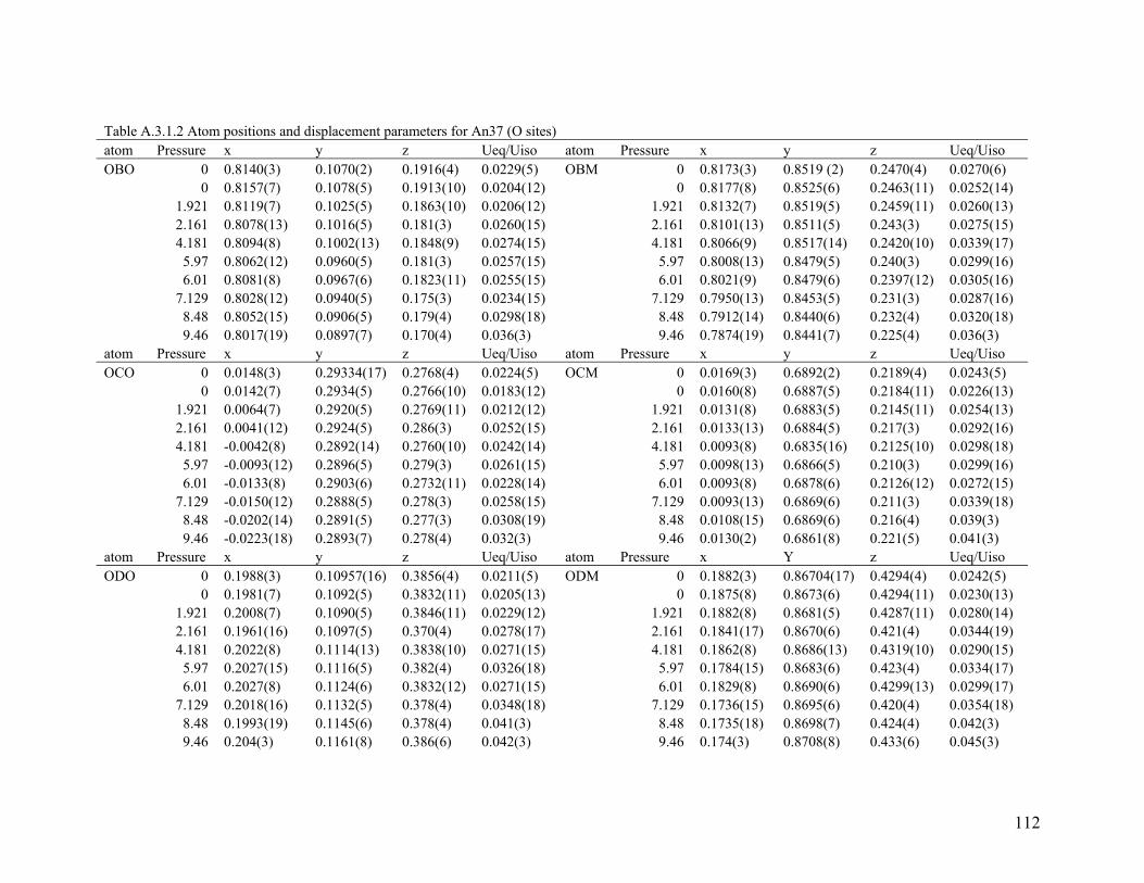
Table A.3.1.2 Atom positions and displacement parameters for An37 (O sites) atom Pressure x y z Ueq/Uiso atom Pressure x y z Ueq/Uiso OBO 0 0.8140(3) 0.1070(2) 0.1916(4) 0.0229(5) OBM 0 0.8173(3) 0.8519 (2) 0.2470(4) 0.0270(6) 0 0.8157(7) 0.1078(5) 0.1913(10) 0.0204(12) 0 0.8177(8) 0.8525(6) 0.2463(11) 0.0252(14) 1.921 0.8119(7) 0.1025(5) 0.1863(10) 0.0206(12) 1.921 0.8132(7) 0.8519(5) 0.2459(11) 0.0260(13) 2.161 0.8078(13) 0.1016(5) 0.181(3) 0.0260(15) 2.161 0.8101(13) 0.8511(5) 0.243(3) 0.0275(15) 4.181 0.8094(8) 0.1002(13) 0.1848(9) 0.0274(15) 4.181 0.8066(9) 0.8517(14) 0.2420(10) 0.0339(17) 5.97 0.8062(12) 0.0960(5) 0.181(3) 0.0257(15) 5.97 0.8008(13) 0.8479(5) 0.240(3) 0.0299(16) 6.01 0.8081(8) 0.0967(6) 0.1823(11) 0.0255(15) 6.01 0.8021(9) 0.8479(6) 0.2397(12) 0.0305(16) 7.129 0.8028(12) 0.0940(5) 0.175(3) 0.0234(15) 7.129 0.7950(13) 0.8453(5) 0.231(3) 0.0287(16) 8.48 0.8052(15) 0.0906(5) 0.179(4) 0.0298(18) 8.48 0.7912(14) 0.8440(6) 0.232(4) 0.0320(18) 9.46 0.8017(19) 0.0897(7) 0.170(4) 0.036(3) 9.46 0.7874(19) 0.8441(7) 0.225(4) 0.036(3) atom Pressure x y z Ueq/Uiso atom Pressure x y z Ueq/Uiso OCO 0 0.0148(3) 0.29334(17) 0.2768(4) 0.0224(5) OCM 0 0.0169(3) 0.6892(2) 0.2189(4) 0.0243(5) 0 0.0142(7) 0.2934(5) 0.2766(10) 0.0183(12) 0 0.0160(8) 0.6887(5) 0.2184(11) 0.0226(13) 1.921 0.0064(7) 0.2920(5) 0.2769(11) 0.0212(12) 1.921 0.0131(8) 0.6883(5) 0.2145(11) 0.0254(13) 2.161 0.0041(12) 0.2924(5) 0.286(3) 0.0252(15) 2.161 0.0133(13) 0.6884(5) 0.217(3) 0.0292(16) 4.181 -0.0042(8) 0.2892(14) 0.2760(10) 0.0242(14) 4.181 0.0093(8) 0.6835(16) 0.2125(10) 0.0298(18) 5.97 -0.0093(12) 0.2896(5) 0.279(3) 0.0261(15) 5.97 0.0098(13) 0.6866(5) 0.210(3) 0.0299(16) 6.01 -0.0133(8) 0.2903(6) 0.2732(11) 0.0228(14) 6.01 0.0093(8) 0.6878(6) 0.2126(12) 0.0272(15) 7.129 -0.0150(12) 0.2888(5) 0.278(3) 0.0258(15) 7.129 0.0093(13) 0.6869(6) 0.211(3) 0.0339(18) 8.48 -0.0202(14) 0.2891(5) 0.277(3) 0.0308(19) 8.48 0.0108(15) 0.6869(6) 0.216(4) 0.039(3) 9.46 -0.0223(18) 0.2893(7) 0.278(4) 0.032(3) 9.46 0.0130(2) 0.6861(8) 0.221(5) 0.041(3) atom Pressure x y z Ueq/Uiso atom Pressure x Y z Ueq/Uiso ODO 0 0.1988(3) 0.10957(16) 0.3856(4) 0.0211(5) ODM 0 0.1882(3) 0.86704(17) 0.4294(4) 0.0242(5) 0 0.1981(7) 0.1092(5) 0.3832(11) 0.0205(13) 0 0.1875(8) 0.8673(6) 0.4294(11) 0.0230(13) 1.921 0.2008(7) 0.1090(5) 0.3846(11) 0.0229(12) 1.921 0.1882(8) 0.8681(5) 0.4287(11) 0.0280(14) 2.161 0.1961(16) 0.1097(5) 0.370(4) 0.0278(17) 2.161 0.1841(17) 0.8670(6) 0.421(4) 0.0344(19) 4.181 0.2022(8) 0.1114(13) 0.3838(10) 0.0271(15) 4.181 0.1862(8) 0.8686(13) 0.4319(10) 0.0290(15) 5.97 0.2027(15) 0.1116(5) 0.382(4) 0.0326(18) 5.97 0.1784(15) 0.8683(6) 0.423(4) 0.0334(17) 6.01 0.2027(8) 0.1124(6) 0.3832(12) 0.0271(15) 6.01 0.1829(8) 0.8690(6) 0.4299(13) 0.0299(17) 7.129 0.2018(16) 0.1132(5) 0.378(4) 0.0348(18) 7.129 0.1736(15) 0.8695(6) 0.420(4) 0.0354(18) 8.48 0.1993(19) 0.1145(6) 0.378(4) 0.041(3) 8.48 0.1735(18) 0.8698(7) 0.424(4) 0.042(3) 9.46 0.204(3) 0.1161(8) 0.386(6) 0.042(3) 9.46 0.174(3) 0.8708(8) 0.433(6) 0.045(3)

112

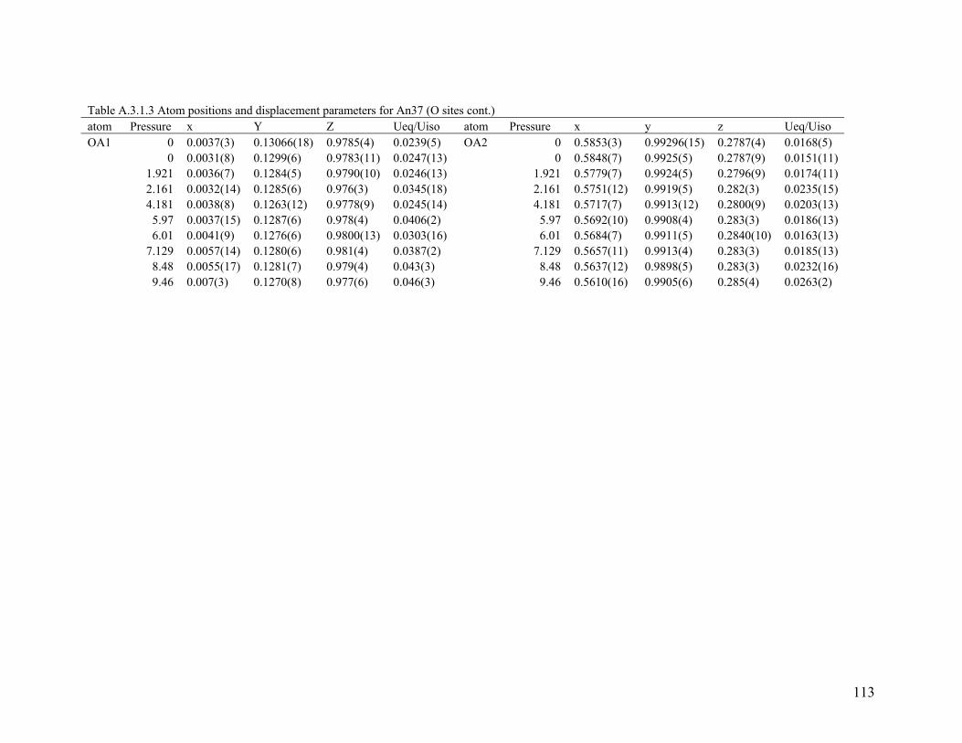
Table A.3.1.3 Atom positions and displacement parameters for An37 (O sites cont.) atom Pressure x Y Z Ueq/Uiso atom Pressure x y z Ueq/Uiso OA1 0 0.0037(3) 0.13066(18) 0.9785(4) 0.0239(5) OA2 0 0.5853(3) 0.99296(15) 0.2787(4) 0.0168(5) 0 0.0031(8) 0.1299(6) 0.9783(11) 0.0247(13) 0 0.5848(7) 0.9925(5) 0.2787(9) 0.0151(11) 1.921 0.0036(7) 0.1284(5) 0.9790(10) 0.0246(13) 1.921 0.5779(7) 0.9924(5) 0.2796(9) 0.0174(11) 2.161 0.0032(14) 0.1285(6) 0.976(3) 0.0345(18) 2.161 0.5751(12) 0.9919(5) 0.282(3) 0.0235(15) 4.181 0.0038(8) 0.1263(12) 0.9778(9) 0.0245(14) 4.181 0.5717(7) 0.9913(12) 0.2800(9) 0.0203(13) 5.97 0.0037(15) 0.1287(6) 0.978(4) 0.0406(2) 5.97 0.5692(10) 0.9908(4) 0.283(3) 0.0186(13) 6.01 0.0041(9) 0.1276(6) 0.9800(13) 0.0303(16) 6.01 0.5684(7) 0.9911(5) 0.2840(10) 0.0163(13) 7.129 0.0057(14) 0.1280(6) 0.981(4) 0.0387(2) 7.129 0.5657(11) 0.9913(4) 0.283(3) 0.0185(13) 8.48 0.0055(17) 0.1281(7) 0.979(4) 0.043(3) 8.48 0.5637(12) 0.9898(5) 0.283(3) 0.0232(16) 9.46 0.007(3) 0.1270(8) 0.977(6) 0.046(3) 9.46 0.5610(16) 0.9905(6) 0.285(4) 0.0263(2)

113

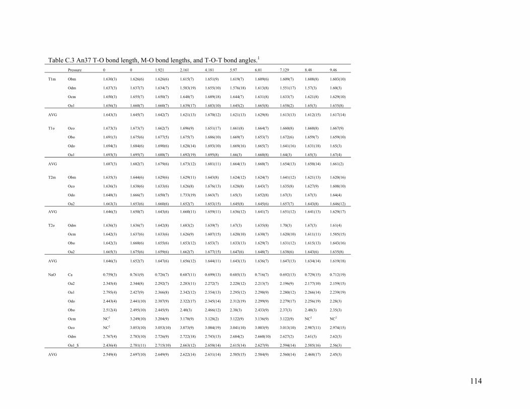
Table C.3 An37 T-O bond length, M-O bond lengths, and T-O-T bond angles.1 Pressure 0 0 1.921 2.161 4.181 5.97 6.01 7.129 8.48 9.46

T1m Obm 1.630(3) 1.626(6) 1.626(6) 1.615(7) 1.651(9) 1.619(7) 1.609(6) 1.609(7) 1.608(8) 1.603(10)

Odm 1.637(3) 1.637(7) 1.634(7) 1.583(19) 1.655(10) 1.576(18) 1.613(8) 1.551(17) 1.57(3) 1.60(3)

Ocm 1.650(3) 1.655(7) 1.650(7) 1.648(7) 1.689(18) 1.644(7) 1.631(8) 1.633(7) 1.621(8) 1.629(10)

Oa1 1.656(3) 1.660(7) 1.660(7) 1.639(17) 1.683(10) 1.645(2) 1.665(8) 1.658(2) 1.65(3) 1.635(8)

AVG 1.643(3) 1.645(7) 1.642(7) 1.621(13) 1.670(12) 1.621(13) 1.629(8) 1.613(13) 1.612(15) 1.617(14)

T1o Oco 1.673(3) 1.673(7) 1.662(7) 1.696(9) 1.651(17) 1.661(8) 1.664(7) 1.660(8) 1.660(8) 1.667(9)

Obo 1.691(3) 1.675(6) 1.677(5) 1.675(7) 1.686(10) 1.669(7) 1.653(7) 1.672(6) 1.659(7) 1.659(10)

Odo 1.694(3) 1.684(6) 1.690(6) 1.628(14) 1.693(10) 1.669(16) 1.665(7) 1.641(16) 1.631(18) 1.65(3)

Oa1 1.693(3) 1.695(7) 1.688(7) 1.692(19) 1.695(8) 1.66(3) 1.660(8) 1.64(3) 1.65(3) 1.67(4)

AVG 1.687(3) 1.682(7) 1.679(6) 1.673(12) 1.681(11) 1.664(13) 1.660(7) 1.654(13) 1.650(14) 1.661(2)

T2m Obm 1.635(3) 1.644(6) 1.629(6) 1.629(11) 1.643(8) 1.624(12) 1.624(7) 1.641(12) 1.621(13) 1.620(16)

Oco 1.636(3) 1.638(6) 1.633(6) 1.626(8) 1.676(13) 1.628(8) 1.643(7) 1.635(8) 1.627(9) 1.608(10)

Odo 1.648(3) 1.666(7) 1.650(7) 1.733(19) 1.663(7) 1.65(3) 1.652(8) 1.67(3) 1.67(3) 1.64(4)

Oa2 1.663(3) 1.653(6) 1.660(6) 1.652(7) 1.653(15) 1.645(8) 1.645(6) 1.657(7) 1.643(8) 1.646(12)

AVG 1.646(3) 1.650(7) 1.643(6) 1.660(11) 1.659(11) 1.636(12) 1.641(7) 1.651(12) 1.641(13) 1.629(17)

T2o Odm 1.636(3) 1.636(7) 1.642(8) 1.683(2) 1.639(7) 1.67(3) 1.635(8) 1.70(3) 1.67(3) 1.61(4)

Ocm 1.642(3) 1.637(6) 1.633(6) 1.626(9) 1.607(15) 1.620(10) 1.630(7) 1.620(10) 1.611(11) 1.585(15)

Obo 1.642(3) 1.660(6) 1.655(6) 1.653(12) 1.653(7) 1.633(13) 1.629(7) 1.631(12) 1.615(13) 1.643(16)

Oa2 1.665(3) 1.675(6) 1.659(6) 1.662(7) 1.677(15) 1.647(6) 1.648(7) 1.638(6) 1.643(6) 1.635(8)

AVG 1.646(3) 1.652(7) 1.647(6) 1.656(12) 1.644(11) 1.643(13) 1.636(7) 1.647(13) 1.634(14) 1.619(18)

NaO Ca 0.759(3) 0.761(9) 0.726(7) 0.687(11) 0.699(13) 0.685(13) 0.716(7) 0.692(13) 0.729(15) 0.712(19)

Oa2 2.345(4) 2.344(8) 2.292(7) 2.283(11) 2.272(7) 2.228(12) 2.213(7) 2.196(9) 2.177(10) 2.159(15)

Oa1 2.795(4) 2.427(9) 2.366(8) 2.342(12) 2.354(13) 2.295(12) 2.298(9) 2.280(12) 2.266(14) 2.239(19)

Odo 2.443(4) 2.441(10) 2.387(9) 2.322(17) 2.345(14) 2.312(19) 2.299(9) 2.279(17) 2.256(19) 2.28(3)

Obo 2.512(4) 2.495(10) 2.445(9) 2.40(3) 2.466(12) 2.38(3) 2.433(9) 2.37(3) 2.40(3) 2.35(3)

Ocm NC2 3.249(10) 3.204(9) 3.178(9) 3.128(2) 3.122(9) 3.136(9) 3.122(9) NC2 NC2

Oco NC2 3.053(10) 3.053(10) 3.073(9) 3.084(19) 3.041(10) 3.003(9) 3.013(10) 2.987(11) 2.974(15)

Odm 2.767(4) 2.783(10) 2.726(9) 2.722(18) 2.743(13) 2.684(2) 2.660(10) 2.627(2) 2.61(3) 2.62(3)

Oa1_$ 2.436(4) 2.781(11) 2.715(10) 2.663(12) 2.658(14) 2.615(14) 2.627(9) 2.594(14) 2.585(16) 2.56(3)

AVG 2.549(4) 2.697(10) 2.649(9) 2.622(14) 2.631(14) 2.585(15) 2.584(9) 2.560(14) 2.468(17) 2.45(3)

114

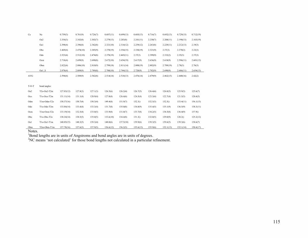
Ca Na 0.759(3) 0.761(9) 0.726(7) 0.687(11) 0.699(13) 0.685(13) 0.716(7) 0.692(13) 0.729(15) 0.712(19)

Oa2 2.354(3) 2.342(8) 2.302(7) 2.279(13) 2.283(8) 2.241(11) 2.230(7) 2.208(11) 2.190(13) 2.163(19)

Oa1 2.398(4) 2.396(8) 2.342(8) 2.321(10) 2.314(12) 2.259(12) 2.263(8) 2.229(11) 2.212(13) 2.19(3)

Obo 2.469(4) 2.478(10) 2.385(9) 2.370(19) 2.354(15) 2.330(19) 2.321(9) 2.37(3) 2.270(2) 2.22(3)

Odo 2.523(4) 2.512(10) 2.474(8) 2.378(19) 2.465(11) 2.37(3) 2.399(9) 2.332(2) 2.35(3) 2.37(3)

Ocm 2.718(4) 2.699(9) 2.690(8) 2.672(10) 2.654(19) 2.617(9) 2.636(9) 2.618(9) 2.596(11) 2.601(13)

Obm 2.822(4) 2.806(10) 2.810(9) 2.799(18) 2.811(14) 2.800(19) 2.802(9) 2.789(19) 2.78(3) 2.76(3)

Oa1_$ 2.878(4) 2.889(9) 2.789(8) 2.780(10) 2.744(15) 2.720(9) 2.702(9) 2.690(9) 2.686(11) 2.654(13)

AVG 2.594(4) 2.589(9) 2.542(8) 2.514(14) 2.518(13) 2.476(14) 2.479(9) 2.462(15) 2.440(16) 2.42(2)

T-O-T bond angles:

Oa2 T2o-Oa2-T2m 127.83(12) 127.8(3) 127.1(3) 126.5(6) 126.2(4) 126.7(5) 126.4(4) 126.0(5) 125.9(5) 125.6(7)

Oco T1o-Oco-T2m 131.11(14) 131.1(4) 128.9(4) 127.0(4) 126.4(6) 124.5(4) 123.3(4) 122.7(4) 121.5(5) 120.4(5)

Odm T1m-Odm-T2o 150.37(16) 150.7(4) 150.3(4) 149.4(8) 151.9(7) 152.3() 152.5(5) 152.5() 153.4(11) 156.1(15)

Odo T1o-Odo-T2m 133.84(14) 133.4(4) 133.3(4) 131.7(8) 135.0(8) 134.8(9) 135.4(5) 135.1(9) 136.5(9) 138.3(11)

Ocm T1m-Ocm-T2o 133.19(14) 132.5(4) 133.0(5) 133.9(8) 131.0(7) 133.7(8) 134.2(5) 134.5(8) 136.4(9) 137.9()

Obo T1o-Obo-T2o 138.24(14) 138.5(5) 135.0(5) 133.6(10) 134.4(8) 131.3() 132.0(5) 129.0(9) 128.2() 125.2(12)

Oa1 T1o-Oa1-T1m 140.85(15) 140.3(5) 139.3(4) 140.0(6) 137.5(10) 139.9(6) 139.3(5) 139.6(5) 139.3(6) 138.6(7)

Obm T2m-Obm-T1m 157.78(16) 157.6(5) 157.9(5) 156.6(12) 156.2(5) 155.6(13) 155.9(6) 152.1(13) 152.1(14) 150.4(17)

Notes. 1Bond lengths are in units of Angstroms and bond angles are in units of degrees. 2NC means ‘not calculated’ for those bond lengths not calculated in a particular refinement.

115