The effects of space-discretizations on computing inertial...

THE EFFECTS OF SPACE-DISCRETIZATIONS

ON COMPUTING INERTIAL MANIFOLDS

Konstantinos E. Korontinis

B.Sc., Simon Fraser University, Burnaby, 1989

THESIS SUBMITTED IN PARTIAL FULFILMENT OF

THE REQUIREMENTS FOR THE DEGREE OF

MASTER OF SCIENCE

in the Department

of

Mathematics and Statistics

OKonstantinos E. Korontinis

SIMON FRASER UNIVERSITY

May, 1992

All rights reserved. This work may not be reproduced in whole or in part, by photocopy

or other means, without permission of the author.

Approval

Name : Konstantinos E. Korontinis

Degree : Master of Science

Title of Thesis : The Effects of Space-discretizations on Computing Inertial Manifolds

Examining committee :

Chairman: Dr. A. Lachlan

Dr. M.R. Trummer

Senior Supervisor

., Dr. R.D. Russell

1 I

Dr. T . T&ng

Dr. E. V a n Vleck

External Examiner Department of Mathematics and Statistics Simon Fraser University

Date Approved : May 21, 1992

PARTIAL COPYIIIGIiT LICLNSC:

I hereby g ran t t o Simon Frasei- IJn ivcrs i f y t l i ~ r i g h l . 1.0 lend

my thesis, p r o j e c t o r extended essay ( t h o t i t l a o f which i s shown below)

t o users o f the Simon Frasor U n i v e r s i t y L ibrary, and t o make p a l - t i a l o r

s ing le copies on ly f o r such users o r i n response t o a request from t h e

l i b r a r y o f any o the r un ivers i ty , . o r o the r educational i n s t i t u t i o n , on

' i t s own behalf o r f o r one of i t s users. I f u r t h e r agree t h a t permission

. f o r m u l t i p l e copying of t h i s work f o r r ;chol i t r ly purposes may be gran'ted

by me o r the Doan o f Graduate Studies. I t i s understood t h a t copying

or pub1 l c a t i o n o f t h i s work f o r f i n a n c i a l ga in s h a l l not be a l lowed

wi thout my w r i t t e n permission.

. .. T i t l e o f Thesis/Project/Extendod Essay . ,

Author :

(s ignature)

,9 IQ92. -. . (date)

Abstract

In this thesis we investigate various aspects of the problem of computing inertial

manifolds for dissipative Partial Differential Equations (PDEs). In particular, we in-

vestigate cases where only an approximate spectral decomposition of the dominant

differential operator is known. We perform numerical experiments in one space di-

mension by discretizing the space variable and performing all of the computations on

a fine grid. Furthermore, we approximate the first few of the smallest eigenvalues

and eigenvectors of the discretized operator using the Lanczos algorithm. This is the

initial step towards computing inertial manifolds for systems involving more than one

space dimension and irregular domains.

The basic ideas and techniques are exemplified for the Kuramoto-Sivashinsky (KS)

and the Reaction-Diffusion (RD) equations. These equations are chosen because they

are fairly simple but their dynamics are sufficiently complicated, and they are a clas-

sical case for which a considerable amount of computational experience has been

documented.

Our results are compared to those for other methods where the exact eigenvalues

and eigenvectors are used. This comparison is not meant to test the competitiveness

of the discrete method since, for the case tested, the other methods are expected to

be better. Rather, it is a test study to show that the discrete method can be used as

a general method for computing inertial manifolds.

Dedication

To Litsa, whose continuous support has been invaluable.

Acknowledgments

The completion of this thesis would not have been possible without the support

of many people.

I am deeply grateful to my senior supervisor Dr. M. R. Trumrner for his continuous

academic support, patience and friendship from the beginning of my graduate studies.

I also owe special thanks to him for trusting my abilities during the initial period of

this program.

I am equally grateful to Dr. R. D. Russell whose long time friendship and encour-

agement played an important role in my decision to pursue graduate studies.

I also wish to express my appreciation to Dr. E. Van Vleck for his questions and

comments, especially on the early drafts of this work.

Many thanks to my family and to my friends Thanasis Passias, Antonio Cabal

and Roger Coroas, whose consistent moral support helped me tremendously.

I would also like to express my thanks to Sylvia Holmes and Tasoula Berggren

for their assistance, and to the Department of Mathematics and Statistics of Simon

Fraser University for financial support.

Contents

1 Introduction 1

2 General Theory 3

. . . . . . . . . . . . . . . . . . . . . . . . . . . 2.1 The General Problem 3

2.2 Inertial Manifolds . . . . . . . . . . . . . . . . . . . . . . . . . . . . . 4

. . . . . . . . . . . . . . . . . . . . . 2.3 Approximate Inertial Manifolds 5

. . . . . . . . . . . . . . . . . 2.4 Existence theories for inertial manifolds 7

3 Approximate Inertial Manifolds 8

3.1 Euler . Galerkin . . . . . . . . . . . . . . . . . . . . . . . . . . . . . . 8

. . . . . . . . . . . . . . . . . . . . . . . . . . . . . 3.2 TheSteadyAIM 10

4 The Discrete Method 13

. . . . . . . . . . . . . . . . . . . . . . . . . . 4.1 Examples considered 14

. . . . . . . . . . . . . . . . . . . . . . . . . . . 4.2 The Lanczos Method 20

5 Numerical Results 28

. . . . . . . . . . . . . . . . . . . . . . . . . . 5.1 Steady-State Solutions 29 . . . . . . . . . . . . . . . . . . . . . . . . . . . . . 5.2 Periodic Solutions 31

. . . . . . . . . . . . . . . . . . 5.3 Variable Number of Picard Iterations 33 . . . . . . . . . . . . . . . . . . . . . . . . . . . . . . . . 5.4 Conclusions 35

List of Tables

5.1 CPU times for the Flat-Galerkin methods . . . . . . . . . . . . . . . . 30

5.2 CPU time for the Non-linear Galerkin with p + q = 5 + 5 modes and

its = 6 Picard iterations . . . . . . . . . . . . . . . . . . . . . . . . . . 30

5.3 CPU time for the Discrete method with its = 6 iterations . . . . . . . 31

5.4 CPU time for periodic solutions with p + q = 5 + 5 modes and its = 6

Picard iterations . . . . . . . . . . . . . . . . . . . . . . . . . . . . . . 5.5 CPU time for the Discrete method with variable Picard iterations . . 34

vii

... V l l l

List of Figures

Figure la: 12 modes. Flat.Galerkin. RST ................................... 37

Figure lb: 12 modes. Flat.Galerkin. Discrete ................................ 37

Figure 2a: 5+5. Nonlinear. Discrete. i ts = 6 ................................. 38

Figure 2b: 5+5. Nonlinear. RST.Newton. i ts = 6 ............................ 38

Figure 3a: 4+4. Nonlinear. Discrete. i ts = 6 ................................. 39

Figure 3b: 6+6. Nonlinear. Discrete. i ts = 6 ................................. 39

Figure 4a: 5+5. Nonlinear. Periodic. Discrete. its = 6 ....................... 40

Figure 4b: 5+5. Nonlinear. Periodic. Discrete. i ts = 6 ....................... 40

Figure 5a: 5+5. Variable Picard iterations ................................... 41

Figure 5b: 5+5. Variable Picard . Periodic .................................. 41

Figure 6a: 6+6. Discrete. including "spurious" .............................. 42

........................................... Figure 6b: 5+5. Discrete. N = 64 42

Figure 7a: 12 modes. Flat.Galerkin. RD equation ........................... 43

Figure 7b: 5+5. RD equation. Nonlinear. its = 6 ............................ 43

Chapter 1

Introduction

Recently there has been considerable interest, especially in the dynamical systems

community, in the computation of inertial manifolds for dissipative partial differential

equations (PDEs). This process is carried out by first splitting the solution space H

into two subspaces PH and QH, where P is an orthogonal projection on H with finite

dimensional range and Q = I-P. To date, the methods used to compute inertial man-

ifolds have dealt with cases where these projections are based on eigenfunctions that

are known. This restricts the application of these methods mostly to one-dimensional

problems or regular domains. Because many problems arising in practice do not fit

in this framework, a method that can be adapted to higher dimensional problems or

to one dimensional problems with more complicated boundary conditions is needed.

In this thesis we make a first step in this direction by developing a method that

we believe can be adapted to situations involving more than one space dimension and

irregular domains. In the discrete method we apply two ideas: First we discretize

the space variable creating a computational grid and also, we approximate, using the

Lanczos iteration, the eigenvalues of the discretized operator.

CHAPTER 1. INTRODUCTION

For comparison purposes, we test our method on one space dimensional equa-

tions for which exact eigenfunctions are known. These equations are the Kuramoto-

Sivashinsky (KS) and the Reaction-Diffusion (RD) equations. We compare our results

to two methods developed by Russell, Sloan and Trumrner in [RSTl], by investigat-

ing how accurately and how efficiently the discrete method describes the qualitative

behaviour of the KS equation as it is demonstrated in its bifurcation diagram.

It should be pointed out that the discrete method is not designed to be compet-

itive in cases where the exact eigenfunctions are known, but rather, to be applied to

problems over irregular domains where the eigenfunctions of the operator can only be

approximated. Therefore, we do expect a loss of efficiency. However, it is interest-

ing to note that experiments indicate that the discrete method might be somewhat

more robust than the semi-discrete methods used in [RSTl] and [JKTl]. It is also

worthwhile mentioning that the treatment of nonlinear terms is much simpler for the

discrete method.

In the second chapter we discuss some of the general inertial manifold theory

and give some basic definitions. In chapter three we describe briefly the existing

methods to approximate inertial manifolds, while in chapter four we describe the

discrete method as it is applied to the KS equation. We also describe the Lanczos

algorithm, which is the method used to approximate the first m smallest eigenvalues

and corresponding eigenvectors. In chapter five we discuss the numerical results that

we obtained after applying the discrete method and we compare our method to the

methods developed in the paper [RSTl].

Chapter 2

General Theory

2.1 The General Problem

Consider the evolution equation of the form

ut + Au + F(u) = 0

where A is a self-adjoint positive operator with compact resolvent defined on a Hilbert

space H, and F(u) is the nonlinear part defined on the domain of A.

A is usually a (dissipative) spatial differential operator (like the Laplacian, or the

biharmonic operator), making (2.1) a partial differential equation (PDE). Let u(t) = S(t)uo denote the solution to (2.1) at time t satisfying the initial

condition u(to) = uo.

Assume that the above evolution equation is dissipative, i. e., its trajectories enter

and eventually remain in an absorbing ball contained in the appropriate phase space.

That is, the solution map uo -+ u(t) = S(t)uo satisfies the following property:

There exists a compact, convex set Y c H such that, for any bounded set

X c H there exists to = to(X) with S(t)uo E Y for all t 2 to, uo E X.

CHAPTERZ. GENERAL THEORY

The operator A has a complete orthogonal set of eigenfunctions wl, w2,. . . , with

corresponding eigenvalues 0 < XI 5 X2 5 . . . . Define P to be the spectral projection onto the span of the first n eigenfunctions

and Q := I - P be that onto the remaining ones, i. e.,

and

where ( , ) denotes the scalar product on H.

2.2 Inertial Manifolds

Definition : A subset R c H is said to be an inertial manifold for equation (2.1)

if 0 satisfies the following conditions:

1. 0 is a finite dimensional Lipschitz manifold in H

2. fl is positively invariant, i. e., if uo E R then S(t)uo E R for all t > 0.

3. R is exponentially attracting, i. e., there is a p > 0 such that for every uo E H

there is a constant K = K(uo) such that dist(S(t)uo, fl) 2 Ke-fit, t > 0.

Existence of an inertial manifold is very important since it implies that the dy-

namics of the original equation (2.1) are completely described by a finite dimensional

ordinary differential equation (ODE), with no error.

A brief description of existence theories for inertial manifolds will come in a later

section; for now we concentrate on how to obtain the reduced system of ODES.

Assuming that the eigenvalues of A grow sufficiently fast to satisfy a gap condition

[LS], it is possible to obtain an upper bound on n such that fl is the graph of a

smooth function

Q , : P H - , Q H .

CHAPTER 2. GENERAL THEORY

Recall that PH and QH are subspaces of the solution space H with P and Q being

the orthogonal projections on H as defined in the previous section.

Under the above assumptions the graph of the function is an n-dimensional

manifold in H.

For u E H we set p = P u , q = Qu, and using the commutivity relations P A = A P

and Q A = A Q we can write the PDE (2 .1 ) equivalently as the following system of

ODEs

p + A P p + P F ( p + q ) = O (2 .4 )

By expressing the q variables in terms of the p variables through the relation

q = @ ( p ) we obtain the following reduced system of ODEs

which can now be used to determine the long-term dynamics of the original equation

with no error. The system (2 .6 ) is called an inertial form of (2 .1) .

2.3 Approximate Inertial Manifolds

Note that the way P and Q are defined in (2 .2) and (2 .3 ) , P is an orthogonal projec-

tion on H with finite dimensional range, while Q has, infinite dimensional range. In

practice Q is approximated by truncating the series (2 .3 ) and therefore equation (2 .3) is replaced by

Because of this truncation, the relation between p and q is replaced by an approx-

imation, say 4 , ( ~ ) which now maps PH into the finite dimensional space QH, and

the corresponding graph 0, is now an approximate inertial manifold (AIM) of (2 .1) .


From now on it is assumed that the truncation has taken place, thus the subscript is

dropped and R denotes an AIM.

In order to determine the long-term dynamics of the dissipative PDE (2.1), we

need to compute solutions of the ODE system (2.6) and this requires computing the

function 4. There are a number of ways to do this, some of which will be discussed

below:

Galerkin approximations. The classical (or flat) Galerkin approximation in-

volves setting the function q = +(p) r 0. Then the system (2.6) becomes

which now is a system of ODES dependent only on the variable p and can be solved

using the standard techniques.

The modified (or nonlinear) Galerkin approximations involve a nontrivial approx-

imation to 4, say $,(p), in equation (2.4) to get

There are many ways to obtain approximations to 4 which can be divided into

two groups:

1. Solve a PDE for 4(p) using both equations (2.4) and (2.5)

2. Use (2.5) to find an approximation to 4(p) and then use it in (2.4).

In this thesis only methods which belong to the second group will be discussed.

The Euler-Galerkin approximation involves starting with the flat manifold, i. e.,

Now, under appropriate assumptions, it can be shown, [FST], that as t + oo the semi-

flow induced by the solution of (2.1) takes the initial manifold Ro to a true inertial

manifold R through the relation Rt = S(t)Ro. Since R is exponentially attracting,

after a relatively short time interval T , R,, the image under the semi-flow of 00, can


be shown to be very close to fl, [FST]. The key to this approach is to approximate

the true evolution with the implicit Euler method for small time T.

Other methods to approximate inertial manifolds include elliptic regularization

and parabolic regularization. For more details on these and on the above described

methods the reader can look in [LS] and in the references given therein.

2.4 Existence theories for inertial manifolds

There are three classes of existence theories for inertial manifolds.

The Lyapunov-Perron method is based on the variation of constants formula.

This method is very useful for deriving properties of inertial manifolds and for proving

existence but it does not appear to be a good method for approximating one. The

reason for this is that it uses backward integration of the equation which is the unstable

direction.

The second class of theories uses the Hadamard (or graph transform) method.

The basic idea behind this method is to start with an initial approximation to the

manifold, say no. Then, by letting the dynamics of the evolutionary equation act on

Ro we get a set Rt at each time t > 0. Under suitable hypotheses, it can be proven

that each Rt is representable as the graph of some function, the limit

lim Rt = $2 t+m

exists and that f l is the inertial manifold.

The last class of existence theories is based on the method of elliptic regular-

ization developed by Sacker [Sl],[S2]. The extension of the above method to infinite

dimensional dynarnical systems is presented in [LS].

For more details on the above theories the reader is referred to [LS] .

Chapter 3

Approximate Inertial Manifolds

In this chapter we discuss some of the methods which have been used to approximate

inertial manifolds. Recall from chapter 2 the system of ODES

and

Q + A Q q + Q F ( p + q ) = O .

Our goal is to determine the relation q = q 5 ( ~ ) from equation (3 .2) for q and then

use this relation to solve the system

3.1 Euler - Galerkin

This method is based on the Hadamard approach to prove existence of inertial man-

ifolds. The basic idea behind this approach is to start with the flat manifold as the

initial manifold, i. e.,

R o = { u = p + q : q = O ) C H (3.4)

CHAPTER 3. APPROXIMATE INERTIAL MANIFOLDS

and set Rt = S(t)Ro.

Then Rt is a subset of H and under appropriate assumptions, [CFNT1,2], it can

be represented as the graph of a function

where Qt : P H -, QH is a Lipschitz continuous function. Furthermore it can be

shown that the limit

lim qt = @ t--roo

exists, and R = Graph@ is an inertial manifold [M-PS],[CFNTl], [FST].

More specifically, under certain assumptions and for some relatively short time

interval T , one can show that

for every E. > 0, [LS].

The Euler-Galerkin method for approximating inertial manifolds uses the implicit

Euler method to approximate W . In the paper [FJKST], which first introduced

several of these general methods for computing inertial manifolds, the Backward Euler

method with one iteration is used, taking q = 0 as the initial approximation.

Let (po, qo) be a given initial condition and let (p(r), q ( ~ ) ) denote the correspond-

ing solution of the system (3.1) and (3.2) at t = T. The implicit Backward Euler

approximation (pa (T), qa (7)) is given by letting pa (t) be the solution of

with p(0) = po, and then setting

(It should be noted that in the [FJKST] paper equation (3.7) was not solved

but a constant value for p,(t) was assigned instead. That is, in equation (3.8) the

value pa (T) = po was used. The same approach has been used thus far with the other


methods as well. A point of interest would be to see whether there would be improved

results for the Backward Euler method if pa( t ) was also being updated at each step).

Since the mapping po -+ p = p a ( r ) is a homeomorphism of PH, and since qo = 0

we get from equation (3 .8)

Applying one iteration with starting value q a ( r ) = 0 we get

Thus, the approximation by the Euler - Galerkin method is q = @ a ( p o ) := q a ( ~ ) ;

using p a ( r ) = po = p this simplifies to

For the above equation the choice of the stepsize T is not obvious. While for An+1

sufficiently large the choice T = l / A n + l can be given some theoretical justification, an

illustration of the practical difficulties one can face can be found in [RSTl].

3.2 The Steady AIM

Another method for approximating $(p) due to Titi [TI is letting q = 0 in equation

(3.2) to obtain:

G ( q ) := A&q + Q F ( p + q ) = 0 . (3.14)

The above equation defines the steady approximate inertial manifold, a,, with

graph q = d , ( p ) .


The idea in this method is to solve the semi-explicit differential algebraic equa-

tions, (DAE), (3.3) and (3.14) to obtain the AIM. Using equation (3.14) we find an

approximation to q = 4,(p) and then we use this approximation in equation (3.3).

The above approximation gives useful results in practice as it is shown in [JKT1,2].

One reason for this is that the AIM obtained from solving the equation (3.14) contains

all exact steady-state solutions involving only the first m modes, so the bifurcation

diagram for the AIM gives a good representation of the steady-state solutions for the

inertial manifold if one exists for these m modes [RSTl].

One method used to solve equation (3.14) is the Picard iteration

with starting value q0 = 0, [JKTl].

Using two iterations in (3.15) gives rise to the so-called pseudo-steady solution and

the corresponding pseudo-steady AIM, fie, the graph of q = $;(p). The latter method

is used in [JKT1,2] with the specific choice rn = 4n, where m - n is the number of

the q modes while n is the number of the p modes, for a quadratic nonlinearity

F(u). The corresponding choice for a nonlinearity of degree r is m = nr2.

We can also use Newton's method to solve equation (3.14). Taking the derivative

with respect to q in equation (3.14) we have

The Newton iteration step is

where J = Q g ( p + qold).

The matrix on the left hand side of equation (3.17) is the trailing principal sub-

matrix of dimension m - n of the Jacobian of the full nonlinear system corresponding \

to the system of equations (3.1) and (3.2) with p = 0, q = 0, [RSTl].

The applicability of this method depends on the structure of the Jacobian matrix.

For some equations, such as the KS equation, the Jacobian has a very simple structure


and thus it is easy and cheap to calculate. But this is not always the case. For more

information on the conditions required for such a property, the reader is referred to

the paper [RST2].

Chapter 4

The Discrete Method

In this chapter we apply the discrete method to specific examples, namely the Reaction-

Diffusion (RD) and the Kuramoto-Sivashinsky (KS) equations. We describe it s imple-

mentation for the calculation of the inertial manifold and we also discuss the Lanczos

method for approximating the eigenvalues and eigenfunctions of the operator A. Most of the methods used to investigate inertial manifolds, including the ones

discussed in the previous chapter, have thus far dealt with cases where the solution

space is partitioned using projections based on eigenfunctions which are known ex-

actly. This is not generally the case, especially when more than one space dimension

and irregular domains are involved. To overcome the above obstacle, one needs a

method where an approximation to the eigenfunctions is used. The discrete method

is a first step in the development of such a method, since we have used an approxima-

tion of the eigenfunctions of the operator A. Also, the use of a discretization makes

easier the calculation of the nonlinearity in the dissipative evolutionary equation at

hand.

The discrete method is applied in two stages. In the first stage we approximate the

first few smallest eigenvalues and corresponding eigenfunctions of A (or more precisely,

a discrete approximation of A). These discrete approximations are then used in a fully

CHAPTER 4. THE DISCRETE METHOD

discrete scheme in the second stage to calculate the inertial manifold.

Note that for dissipative systems under the appropriate assumptions, the energy

contained in the modes with high wave numbers is exponentially dissipated and as-

symptotically very small [JKTl]. This implies that only a few of the smallest eigen-

values are needed.

For the first stage of our method we use the Lanczos algorithm to approximate the

eigenvalues and eigenfunctions of A. The reason for choosing the above algorithm is

that we can calculate the first few small eigenvalues of A without having to compute all

of them. This is very important especially when N, the number of the grid points, is

large and the application of met hods that calculate the full spectrum of the eigenvalues

of A becomes very expensive and therefore impractical.

To test our method we chose the (KS) and the (RD) equations for two reasons.

First they are fairly simple equations but their dynamics are sufficiently complicated

and second, there has been a considerable amount of computational experience col-

lected for both equations.

4.1 Examples considered

The equations that we applied our method to are:

The Kuramoto-Sivashinsky (KS) equation

subject to the periodic boundary conditions

u(x, t ) = u(x + 275 t)

and the restriction of the solution space to odd functions

u(x,t) = -u(2.rr - x, t).

The Reaction-Diffusion (RD) equation (or Chafeey-Infante equation)


subject to the Dirichlet boundary conditions

u(0,t) = u(7r,t) = 0.

Comparing the above equations to the general evolutionary equation

ut + Au + F(u) = 0

we see that for the (KS) equation

Au = 4u,,,,

under the conditions

while, for the (RD) equation

Au = -vu,,

and

F(u) = u3 - u

under the condition

u(0, t) = u(?r, t ) = 0.

Next we show in detail how we apply the fully discrete method to the (KS) equa-

tion. First we explain our method for the flat Galerkin approach and then for the

nonlinear Galerkin approach. In both cases we will assume that we have calculated the

eigenvalues and eigenfunctions of the operator A through Lanczos iteration. Details

on this first stage of our method will be given in a later section.

The general idea of applying the discrete method to the (KS) equation is the

following:


Start off with a uniform grid with grid spacing h = &, and denote the eigenvalues

and eigenvectors of the discretized operator A by A j and wj, respectively, where the

eigenvectors are of the form

The solution u(x, t ) is now also approximated by a vector u = (u1,. . . , U N ) ~ , where

Discretizing the terms u,, and u, by centered differences we have

and 1

u,(ih) E (u,); = h ( ~ i + l - u ; - ~ ) . (4.7)

Let v; := (u,); + u;(u,); denote the ith component of the vector v approximating

the function u,, + uu,. Taking the projection P we find

where y = y (a),

Taking the derivative of the solution with respect to time t we obtain

Substituting in the original equation (KS) we get


Thus, the system of the ODES for the coefficients crj is

at = H(a) (4.10)

It should be noted that we do not take advantage of the special form of the

nonlinearity in the (KS) equation. The calculation of the inertial manifold with the

fully discrete scheme proceeds as follows:

Denote by W the eigenvector matrix with jth column the eigenvector wj corre-

sponding to the jth eigenvalue, j = 1, . . , n. To explain the method, since A is symmetric we assume that the eigenvectors are

normalized such that WTW = I. Note that in the program we have used a different

normalization, W ~ W = 021 where a = this was done to have wj as a discrete

approximation to the function sin(jx) to allow for comparisons with the previously

used spectral approximations.

Define the solution vector u as

u = w . a .

Calculate the vector v at each step by the relation

v; = u;(uz); + ( u X X ) ~ .

L'he projection P v of v onto the range of W can then be computed by

and thus we can now calculate the right hand side of the ODE system given by (4.11).

In the nonlinear case we have to calculate the function q = +(p), where the graph

of 4 is the pseudo-steady AIM, and then solve the equation

CHAPTER 4. T H E DISCRETE METHOD

To calculate q = 4(p) we use the Picard iteration

for a given p and some initial q = qo.

Set

w = [WP w91

and T

a = ( ~ p , ~ q )

where W, = [wl . . w,], Wq = [w,+~ . . w,] with each wj being a vector with N

components, and a, = (al,. . . , an)T, aq = (a,+l,. . . , am)T.

So the notation that we are using is the following: The subscript p indicates the

first n columns of the matrix W which corresponds to p = Pu. The subscript q indi-

cates the remaining m - n columns, i. e., the columns from n + 1 to rn, corresponding

to q = Qu.

Define the solution vector u by

Note that a,, and thus up, does not change during the calculation of the AIM. For some given a, and some initial a, (which can be zero), we start the Picard

iteration loop:

Calculate the function v = u,, + uu, through a finite difference scheme to get the

vector v.

Next calculate the coefficient vector /3 from the relation

and thus, the q components of a using the relation


for j = n + 1 , ..., m.

Next calculate the new solution vector uq = Wq a, and update the solution

End the Picard loop.

Now calculate the vector v = W - 7 for the updated solution and obtain the first

p components of y from the relation

7 = W;.V.

Finally the ODE system in term of the coefficients a is

for j = 1, ..., n. The above system solves the equation

P + AP + PF(P + +(P)) = 0

which describes the inertial form of the original PDE.

To summarize, a general application of the discrete method is as follows:

step 1

Calculate the eigenvalues and eigenfunctions of the matrix operator A using the

Lanczos method and pass the information to step 2.

step 2

Calculate the solution vector u = W . a.

0 Discretize the nonlinear term and then calculate the vector v to obtain the

coefficient vector 7 = wT . v ; W -7 is the projection P v of v onto the range of

W.

If calculating the nonlinear manifold find the relation q = 4 ( p ) using a number

of Picard iterations.

Obtain the ODE system in terms of the coefficients a, that is, at = H(cY).


4.2 The Lanczos Method

In this section we describe the Lanczos method, a technique that can be used to

solve large, sparse, symmetric eigenproblems of the form Ax = Ax. The method

involves partial tridiagonalizations of the given matrix A. The advantages over other

met hods, such as the Householder approach, are that no intermediate full submatrices

are generated and convergence to the extremal eigenvalues of A happens without

needing to complete the tridiagonalization.

Suppose A E IRnXn is large, sparse and symmetric and assume that we want a few

of its largest or smallest eigenvalues. The Lanczos method generates a sequence of

tridiagonal matrices Tj with the property that the extremal eigenvalues of Tj E lR,jXj

are progressively better estimates of A's extremal eigenvalues.

There are many ways to derive the Lanczos algorithm. The way we are going to

proceed is by considering the optimization of the Rayleigh quotient:

The maximum and minimum values of r(x) are An(A) and A1 (A) respectively [GV].

Suppose {qi} C IRn is a sequence of orthonormal vectors and define the scalars Mj

and mj by

Mj = X ~ ( Q ? A Q ~ ) = max yT(QTAQj)y = max ~ ( Q j y ) I An ( A ) (4.13)

Y f O Y ~ Y llY112=1

mj = A, (QTAQ~) = min yT(QTAQj)y = min r(Qjy) 2 A1 ( A ) (4.14)

~ $ 0 Y ~ Y I l ~ l l 2 = 1

where Qj = [ql, ...,qj].

The algorithm is derived by considering how to generate the q j so that Mj and mj

are increasingly better estimates of A,(A) and XI (A).

Suppose vj, uj E span{ql, . . . , qj} are such that Mj = r(uj) and mj = r(vj).

Since r(x) increases most rapidly in the direction of the gradient


we can have Mj+l > Mj if qj+l is determined so that

and similarily, since r(x) decreases most rapidly in the direction of - 61 r ( x ) we want

[GVI. We need to find a qj+l that satisfies the two requirements above. Since ~ r ( x ) E

span{x, Ax), (4.16) and (4.17) are satisfied if

Choose qj+l so K(A, ql, j + 1) = span(ql, . . . , qj+l). Thus, the problem now becomes

computing orthonormal bases for the Krylov subspaces K(A, ql, j). To do this we

look at the connection between the tridiagonalization of A and the QR decomposition

of the Krylov matrix

More specifically, if T = Q T ~ Q is tridiagonal with &el = ql then,

is the QR factorization of K(A, ql, n).

Thus the qj can be generated by tridiagonalizing A with an orthogonal matrix

whose first column is ql. Therefore, to compute the elements of the tridiagonal matrix

T = QTAQ directly we have:

Set

Q = [QI,. . . ,qn]

and - -

T =

Ql P1 . . . 0

W Q2 ". . .

' . . Pn-1

0 -.. a, - -


Multiply both sides of the equation

by Q to get

Q T = A&.

Equating columns on both sides we have

with poqo 0 for j = 1,. . . ,n - 1.

The orthonormality of the q j implies

is nonzero, then qj+l = r j / p j , where pj = f 1 1 rj [ I2 . Organizing the above information we get the Lanczos iteration:

ro = q1 starting vector

Po = 1

qo = 0 j = O

while ,Bj # 0

q j+1 = ~ j l P j

j = j + l

aj = q,TAnj

~j = (A - aj I )q j - pj-lqj-l

P j = I 1 rj 1112

end.

The q vectors are called the Lanczos vectors.


Several mathematical properties of the method are summarized in the following

theorem, the proof of which is given in [GV].

Theorem: Let A E IRnXn be symmetric and assume ql E IRn has unit two-norm.

Then the Lanczos iteration runs until j = m, where m = ranlc(K (A, ql , n)). Moreover,

for j = 1,. . . ,m we have T AQj = QjTj + rjej

has orthonormal columns that span K(A, ql , j) 0.

If the Lanczos vectors are not orthonormal then they do not generate the correct

T matrix. Also, if pj = 0 for some j then the iteration breaks down but not without

giving us some important information. If Pj = 0 then we have calculated an exact

invariant subspace and the eigenvalues of T are the eigenvalues of A, [W].

We can write the tridiagonal eigenvalue problem generated by the Lanczos method

in the form

Tjs = 8s (4.21)

where the 8's are called Ritz values. The Ritz values will approximate the eigenvalues

of A, especially the extremal ones. Approximations to the eigenvectors of A, called

Ritz vectors, can be calculated using the equation

where yi is the Ritz vector corresponding to s;. These Ritz vectors satisfy

Ayi = yiei + rjsj(i) (4.22)


[GVI. In the examples we have used, and specifically for the KS equation , the matrix

operator is as follows:

Discretize the term uxxxx by centered differences to obtain

where h = +. Applying the boundary conditions on the above discretization we have:

1 u(') xxxx = - ( U 3 - + 6u1 - 4u0 + U - 1 )

h4

1 U ( 2 ) - -(u4 - 4 ~ 3 + 6 ~ 2 - 4 ~ 1 + 210) xxxx - h4

Since u is periodic and odd we have u - 1 = - u l , uo = u ~ + l = 0 and u,+2 = - U N .

Applying this we get 1

= i l i ( 5 ~ 1 - 4u2 + u3) u x x x x

1 (3 ) = -(ul - 4u2 + 6u3 - 4 2 4 + u5) u x x x x

h 4


Therefore, the discrete version of the operator A becomes an N x N matrix which

very good. Because the relative spacing of the eigenvalues of A is fairly even through-

we again call A:

out the spectrum, the Lanczos algorithm approximated eigenvalues over the whole

4 A = - h4

spectrum of A. Since our intention is to approximate a few of the smallest eigenval-

ues of A, we applied the algorithm to the inverse of A. The eigenvalues of A-l are

When we applied Lanczos algorithm to the matrix A the initial results were not

- - 5 -4 1 0 0 0 . - - 0

-4 6 -4 1 0 0 . - . 0 1 -4 6 -4 1 0 . . - 0

O 1 -4 6 -4 1 ... O . . ' . ... . 0 ... ... 0 0 1 - 4 5

distributed in a different way. The relative spacing of the largest eigenvalues of A-l

is large, whereas the smaller eigenvalues of A-l are clustered close to 0. Therefore,

the Lanczos method approximates the large eigenvalues of A-' , i. e., the small ones

of A, very well. (Note that A-l is no longer sparse).

In our program we did not actually calculate A-' directly, but we used the

Cholesky decomposition. According to the Cholesky decomposition theorem if A

is positive definite then, it can be decomposed into a product

A = G G ~

'

where G is lower-triangular, in exactly one way. Since A is positive definite, we can

use the above decomposition to obtain the matrix-vector product required in Lanczos

algorithm. The banded structure of A carries over to G.

Recall the two steps of the Lanczos algorithm


Applying A-' instead of A we have

The idea is to substitute the matrix-vector product A-lq by a vector x satisfying

x = A-'q or equivalently

Ax = q (4.24)

and then use forward and backward substitution to solve me system of equations

(4.24). Analytically this is done the following way:

Let A = GGT be the Cholesky decomposition of A. The system (4.24) then be-

comes

G G ~ X = q.

Let y = GTx to get

Gy = q.

Since G is lower-triangular we can solve for y by forward substitution. Once we have

y, we can solve the upper-triangular system GTx = y for x by backward substitution.

After completing the process we have effectively obtained x = A-'q.

One of the biggest drawbacks with the Lanczos algorithm is the problem of "ghost"

or "spurious" eigenvalues. These are multiple eigenvalues of Tj that correspond to

simple eigenvalues of A. They arise when orthogonality of the qj vectors is lost, and

the iteration restarts itself. Thus, while in theory the process should terminate after

n - 1 steps, in practice it continues until we stop it. Some people are using this idea to

calculate not only a few of the extremal eigenvalues but also, the complete spectrum.

It has been observed that the huge tridiagonal matrix Tj has eigenvalues that approx-

imate all eigenvalues of A. The matrix Tj (j >> n) has many more eigenvalues than A

where, the extra eigenvalues are concentrated in tight clusters that approximate the

eigenvalues of A [W].


The way we tried to identify the "spurious" eigenvalues generated by Lanczos

algorithm was to calculate the difference

and keep the eigenval!les and eigenvectors that satisfied a specific tolerance. The

results were slightly inconsistent and further investigation is required. Interestingly

enough, even when we used spurious eigenvalues and eigenvectors in our inertial man-

ifold calculations, the bifurcation diagrams were often hardly affected by the inclusion

of spurious eigenpairs, (see figure 6a).

For more information on how to separate the ghost eigenvalues from the actual

ones see [CW], [KP1,2] and [PR].

Chapter 5

Numerical Results

In this chapter we apply the discrete method to the (KS) equation and compare our

results with those obtained by other methods. Rather than presenting detailed com-

put ations of the AIMS themselves, we concentrate on presenting bifurcation diagrams

obtained via our new discrete method and the previously used "semidiscrete" meth-

ods. All of the computations use an improved version of AUTO, a FORTRAN code

to compute bifurcation diagrams for ODES. AUTO has been developed by Doedel

[Dl, and modified by Liu [LL]. The runs are made on a SUN SPARC station in double

precision (roughly 16 decimal digits) . The bifurcation diagrams show plots of the bifurcation parameter 8 versus the L2-

norm of the solution. Solid lines correspond to stable steady-st ate solutions, broken

lines correspond to unstable ones. White squares denote steady-st ate bifurcation

points, black squares are Hopf bifurcation points, while period doubling points are

marked with two triangles.

The methods that we compare the discrete method to are the ones developed in

the paper [RSTl] and we will denote them by RST-Newton and RST-Picard. RST-

Newton uses the Newton method to solve the equation

CHAPTER 5. NUMERICAL RESULTS

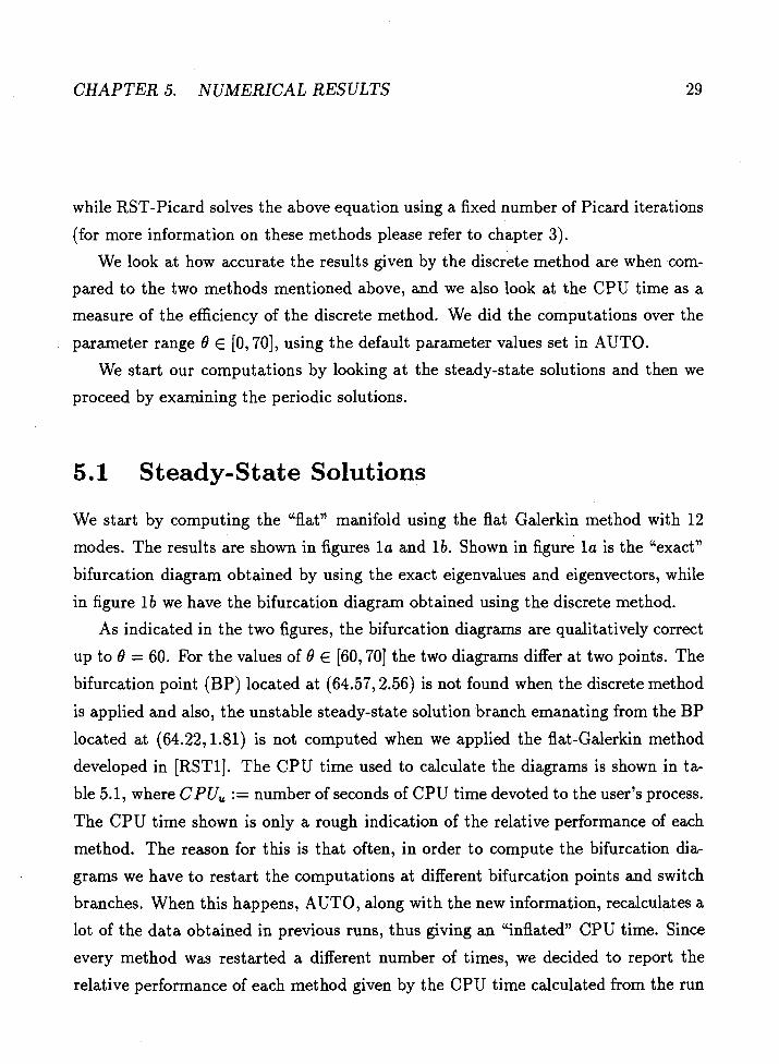
while RST-Picard solves the above equation using a fixed number of Picard iterations

(for more information on these methods please refer to chapter 3).

We look at how accurate the results given by the discrete method are when com-

pared to the two methods mentioned above, and we also look at the CPU time as a

measure of the efficiency of the discrete method. We did the computations over the

parameter range 8 E [O, 701, using the default parameter values set in AUTO.

We start our computations by looking at the steady-state solutions and then we

proceed by examining the periodic solutions.

5.1 St eady-State Solutions

We start by computing the "flatn manifold using the flat Galerkin method with 12

modes. The results are shown in figures l a and lb . Shown in figure l a is the "exact"

bifurcation diagram obtained by using the exact eigenvalues and eigenvectors, while

in figure l b we have the bifurcation diagram obtained using the discrete method.

As indicated in the two figures, the bifurcation diagrams are qualitatively correct

up to 8 = 60. For the values of 8 E [60,70] the two diagrams differ at two points. The

bifurcation point (BP) located at (64.57,2.56) is not found when the discrete method

is applied and also, the unstable steady-state solution branch emanating from the BP

located at (64.22,1.81) is not computed when we applied the flat-Galerkin method

developed in [RSTl]. The CPU time used to calculate the diagrams is shown in ta-

ble 5.1, where CPU, := number of seconds of CPU time devoted to the user's process.

The CPU time shown is only a rough indication of the relative performance of each

method. The reason for this is that often, in order to compute the bifurcation dia-

grams we have to restart the computations at different bifurcation points and switch

branches. When this happens, AUTO, along with the new information, recalculates a

lot of the data obtained in previous runs, thus giving an "inflated" CPU time. Since

every method was restarted a different number of times, we decided to report the

relative performance of each method given by the CPU time calculated from the run


that produced most of the data.

Table 5.1: CPU times for the Flat-Galerkin methods.

In figures 2a and 2b we show the discrete method vs the RST-Newton and RST-

RST-methods

238.8 C PU,

Picard methods using p + q = 5 + 5 modes and a fixed number of Picard iterations,

Discrete method

729.9

its = 6. (The bifurcation diagrams for these two methods for the case where p + q =

5 + 5 modes are identical).

The most noticable difference between these diagrams is again the absence of the

bifurcation point located at (64.57,2.56). In fact, in all the bifurcation diagrams

computed with the discrete method this BP is absent. Also, in the diagrams created

by the RST-methods we could not compute the unstable steady-state solution branch

emanating from the bifurcation point located at (64.22,1.81). It should be noted

however, that only default parameter values were used in AUTO. Often bifurcation

points not found when using these parameter values can be found when re-adjusting

the parameters values. The computation of this branch is shown in the diagrams in

the paper [RSTl]. Comparison of the CPU times is given in table 5.2.

Table 5.2: CPU time for the Non-linear Galerkin with p+q = 5+5 modes and its = 6

I Discrete

CPU, 1 1,152.4

Picard iterations.

In figures 3a and 3b we show bifurcation diagrams obtained from the discrete

RST-Newton

683.6

method using p $ q = 4 + 4 and p + q = 6 + 6 modes respectively, with its = 6 Picard

iterations. The CPU time for these calculations is given in table 5.3; the data suggest

RST-Picard

106.1

that the computational effort for computing diagrams with n + n modes increases

approximately linearly with n.

In all of the results above it is shown that the bifurcation diagrams computed by

the discrete method are very good approximations to the diagrams computed using


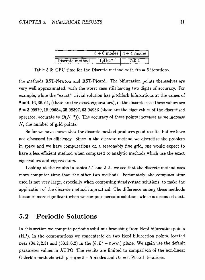
I 1 6 + 6 modes 1 4 + 4 modes I 1 I

I Discrete method 1 1,416.7 740.4 I

Table 5.3: CPU time for the Discrete method with its = 6 iterations.

the methods RST-Newton and RST-Picard. The bifurcation points themselves are

very well approximated, with the worst case still having two digits of accuracy. For

example, while the "exact" trivial solution has pitchfork bifurcations at the values of

0 = 4,16,36,64, (these are the exact eigenvalues), in the discrete case these values are

0 = 3.99979,15.99684,35.98397,63.94933 (these are the eigenvalues of the discretized

operator, accurate to 0 ( N - 2 ) ) . The accuracy of these points increases as we increase

N, the number of grid points.

So far we have shown that the discrete method produces good results, but we have

not discussed its efficiency. Since in the discrete method we discretize the problem

in space and we have computations on a reasonably fine grid, one would expect to

have a less efficient method when compared to analytic methods which use the exact

eigenvalues and eigenvectors.

Looking at the results in tables 5.1 and 5.2 , we see that the discrete method uses

more computer time than the other two methods. Fortunately, the computer time

used is not very large, especially when computing steady-state solutions, to make the

application of the discrete method impractical. The difference among these methods

becomes more significant when we compute periodic solutions which is discussed next.

Periodic Solutions

In this section we compute periodic solutions branching from Hopf bifurcation points

(HP). In the computations we concentrate on two Hopf bifurcation points, located

near (34.2,2.3) and (30.3,6.2) in the (8, L2 - norm) plane. We again use the default

parameter values in AUTO. The results are limited to comparison of the non-linear

Galerkin methods with p + q = 5 + 5 modes and its = 6 Picard iterations.


The solution branches off of the two Hopf bifurcation points are shown in figure 4a,

while finer detail of the periodic solutions generated from the lower Hopf bifurcation

point is shown in figure 4b. One period doubling is found and the corresponding

periodic solution branch is also computed leading into another period doubling. This

second period doubling has not been verified by the RST-Newton or RST-Picard

met hods.

Following the solution branch off of the top Hopf bifurcation point and following

the branch of that point, we find a period doubling. The corresponding periodic

solution branch is also computed and leads to another period doubling (not shown

in this figure here, but calculated in previous computations with p + q = 6 + 6 and

p + q = 4 + 4 modes). These results are consistent with the results found by the

application of the RST-Newton and RST-Picard methods as they are shown in [RSTl].

(With the parameter values used we could not reproduce the finer details calculated

when we follow the branches off the bifurcation point located at (32.79,4.90)).

It is important to note that the results can quickly become sensitive and bifurca-

tion points can be missed or "spurious" ones can appear, and a more detailed study is

required in order to take advantage of changing parameter values in AUTO, such as,

setting smaller tolerances or increasing the number of subintervals for spline colloca-

tion. For more information and more details on AUTO please look at the description

of the method by Doedel, [Dl. The CPU time needed for these calculations is shown

in table 5.4.

Table 5.4: CPU time for periodic solutions with p + q = 5 + 5 modes and its = 6

CPU,

Picard iterations.

As we can see from table 5.4, the amount of computer time increases dramatically

Discrete

5,999.7

when we compute periodic solutions, especially when we follow branches emanating

from period doubling points. The increase of CPU time that occurs when we apply

the discrete method leads us to try and find ways to make the discrete method more

RST-Newton

1,778.8

RST-Picard

389.6


efficient. One such way is, when solving equation (5.1), instead of using q = 0 as an

initial approximation in each step, to use the solution q from the previous parameter

value 8 as an initial approximation to q. This leads us to the next section where we

discuss the discrete method using a variable number of Picard iterations.

Variable Number of Picard Iterations

In this section we discuss the results obtained after applying the discrete method to

the (KS) equation using the non-linear Galerkin approach with p + q = 5 + 5 modes,

with the following variation:

When we solve equation (5.1), instead of using at each step the initial approxima-

tion q = 0 to start the Picard iteration, we use the solution q obtained at the previous

parameter value 8. We let the Picard iteration continue either until it reaches a max-

imum number of iterations previously set, or until the relative difference satisfies a

given tolerance TOL, i. e., until

II qnew - qold / ( 5 TOL. II qnew II

Using the previous value of q instead of q = 0 as an initial approximation reduces

the number of Picard iterations needed, especially when we follow the same branch.

The reason for this is that the values of q change very slowly when we are at the

same branch, so the previous q offers a much better initial approximation for the

Picard iteration for the new value of 0 than q = 0. This way we need very few Picard

iterations to satisfy a given tolerance. The only time we might use the maximum

number of Picard iterations is when we switch branches and the values of q differ a

lot.

In our computations we use as a tolerance the value T OL = 1 .E - 10. This value

was obtained by trial and error. We tried various tolerance values applied to different

number of modes. For instance, when we used p + q = 6 + 6 modes we got fairly good

results with the tolerance set at l.E - 8, while when we used p + q = 4 4 4 modes


Table 5.5: CPU time for the Discrete method with variable Picard iterations.

p + q = 5 + 5 modes

I p + q = 6 + 6 m o d e s

a tolerance of the order l.E - 10 was needed to get some of the results. The CPU

time was also dependent upon the tolerance used. For tolerances of the order or

the CPU time was reduced considerably but at the same time the results were

not very satisfying. Further study is required in order to find the connection between

the parameter values set in AUTO and the value used for the tolerance in the Picard

iteration.

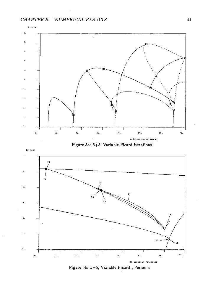
In figures 5a and 5b we show some of the calculations performed on the non-linear

Galerkin case with p+ q = 5 + 5 modes and TO L = 1. E - 10. In figure 5b we show finer

detail of the periodic solutions generated from the top Hopf bifurcation point and of

the two period doublings calculated when we followed the corresponding branches.

The calculations of the periodic solutions generated from the bottom Hopf bifur-

cation point give the same results that we got when we applied the discrete method

to the non-linear Galerkin case with p+q = 5+5 modes and its = 6 Picard iterations

(not shown here). The CPU time used to calculate the two cases is shown in table 5.5.

Notice that if we compare the values obtained for the CPU time from tables 5.2

and 5.5, the discrete method with variable Picard iterations seems to be more ex-

pensive than the one using a fixed number of Picard iterations. It should be pointed

out that when we used the discrete method with a variable number of Picard iter-

ations we got all the information without having to restart AUTO, while when we

used the fixed Picard iterations we needed two more additional runs to complete the

bifurcation diagram. In a similar fashion, looking at table 5.5, the CPU time needed

to do the computations with the p + q = 6 $ 6 modes seems to be very comparable

to the p + q = 5 + 5 case, but additional runs were required in order to complete the

bifurcation diagram.

Tol = l.E - 6

425.4

790.2 -

To1 = l.E - 10 I Tol = l.E - 8

1,549.2

1,598.7

1,111.1

1,419.3


It should be noted that the Picard method with a variable number of iterations can

also be applied to the analytic methods used to compute inertial manifolds. However,

the savings will not be as dramatic as they are for the discrete method.

In figure 6a we show the bifurcation diagram obtained using p + q = 6 + 6 modes

and its = 6 fixed Picard iterations for the non-linear Galerkin method without elimi-

nating all the "spurious" eigenvalues and eigenvectors, while in figure 6b we show the

bifurcation diagram obtained when we use N = 64 grid points for the p + q = 5 + 5

modes and its = 6 Picard iterations. As we can see the qualitative behaviour of

the solution has not been altered dramatically, except for the fact that some of the

bifurcation points were not computed with the AUTO default parameter values. (We

were able to compute some of the missing bifurcation points when we changed some

of the parameter values in AUTO).

Finally, in figure 7 we show the bifurcation diagrams that we obtained when we

applied the discrete method to the Reaction-Diffusion equation. In figure 7a we show

the flat Galerkin approach using 12 modes ,while in figure 7b we show the nonlinear

case using p + q = 5 + 5 modes with its = 6 Picard iterations. Because the RD

equation describes a gradient system we can only have steady-state solutions thus, no

Hopf bifurcation points are detected.

5.4 Conclusions

During the last few years the study of inertial manifolds for dissipative PDEs has been

an active area of research. To date, investigations of inertial manifolds have dealt with

cases where the solution space is partitioned using projections based on eigenfunctions

which can be evaluated exactly and also where the numerical techniques for their

computation have been limited to a fixed number of cycles of a Picard iteration.

In this thesis a first step has been taken towards a different direction. We have

developed a method to compute approximate inertial manifolds under the assumption

that the exact eigenfunctions are not known. Instead, the space variable is discretized


and all of our computations are carried out on a grid. Furthermore, we have shown

how to approximate the first few eigenvalues and eigenvectors of the discrete operator

efficiently using the Lanczos iteration. Using this approach, we showed that AUTO

still produces accurate bifurcation diagrams. The discrete met hod is not designed to

be competitive with methods developed to compute inertial manifolds when the exact

eigenfunctions are available, but rather, to be applied in more general cases where the

eigenfunctions can only be approximated.

Before we can apply our method to cases involving more than one space dimension

and/or irregular domains, we believe that further investigation is needed in order to

computationally improve some aspects of the method. For instance, more research is

needed to find a more efficient and reliable way to identify the "spurious" eigenvalues

and eigenvectors produced by the Lanczos algorithm. It should be noted that an

implementation in higher dimension is by no means a straightforward generalization of

our approach. For example, a non-uniform grid can lead to non-symmetric matrices.

Also, more careful study is required in order to find the best parameter values in

AUTO that combined with the tolerance value given for the Picard iteration will

give the best possible results. Early experiments with the above ideas have led us to

believe that we can optimize the efficiency of the discrete method and therefore, use

it to compute inertial manifolds for more complicated dissipative partial differential

equations.

CHAPTER 5. NUMERICAL RESULTS l , ~ - " < , , m

l l l f u r c a ~ l o n PdranuLor

Figure la: 12 modes, Flat-Galerkin, RST

Bl f u r c a t l o n Paramel c r

Figure lb: 12 modes, Flat-Galerkin, Discrete

CHAPTER 5. NUMERICAL RESULTS I.?-norm

I l l l urcdllon I'dr.lmc~Ler

Figure 2a: 5+5, Nonlinear, Discrete, its = 6

Figure 2b: 5+5, Nonlinear, RST-Newton, its = 6


0. 10. 20. 10. 10. 60.

U l t u r c a l I o n i'aramoler

Figure 3a: 4+4, Nonlinear, Discrete, its = 6

U L C ~ r ~ a t l o n PdI'dmOtOK

Figure 3b: 6+6, Nonlinear, Discrete, its = 6


I.?-norm

UlIurcaLlon Paramotcr

Figure 4a: 5+5, Periodic, Discrete, its = 6

34.50 35 .00 35.50

Figure 4b: 5+5, Periodic, Discrete, its = 6


UI f u r c d t l o n Parameter

Figure 5a: 5+5, Variable Picard iterations

U l I u r c a t l o n I'aramcter

Figure 5b: 5+5, Variable Picard , Periodic

CHAPTER 5. NUMERICAL RESULTS 1.2-norm

O l l u r c a t l o n fr.lrdmoLel

Figure 6a: 6+6, Discrete, including "spurious"

H l f u r c a t l o n parameLer

Figure 6b: 5+5, Discrete, N = 64


I l l furcatJon PardmcLar

Figure 7a: 12 modes, Flat-Galerkin, RD equation

Ill l u r c ~ L l o n pardmclec

Figure 7b: 5+5, RD equation, Nonlinear, its = 6

Bibliography

[CFNTl] P. Constantin, C. Foias, B. Nicolaenko, and R. Temam (1989), Spectral

barriers and inertial manifolds for dissipative partial differential equations, J.

Dynamics & Diff. Eqns. 1, pp 45-73.

[CFNT2] P. Constantin, C. Foias, B. Nicolaenko, and R. Temam (1988), Integral man-

ifolds and inertial manifolds for dissipative partial differential equations, Applied

Mat hematics Sciences, No. 70, (Springer, Berlin).

[CW] J.Cullum and R. A. Willoughby (1978), Lanczos and the computation in speci-

fied intervals of the spectrum of large, sparce real symmetric matrices, in Sparce

Matrix Proc., ed. I. S. Duff and G. W. Stewart, SIAM Publications, Philadelphia,

PA.

[Dl E. J. Doedel (1980), AUTO: A program for the automatic bifurcation analysis of

autonomous systems, Cong. Num. 30 (1981), pp. 265-284, (Proc. 10th Manitoba

Conf. on Num. Math. and Comp., Univ. of Manitoba, Winnipeg, Canada).

[FJKST] C.Foias, M. S. Jolly, I. G. Kevrekidis, G. R. Sell, and E. S. Titi (1988), On

the computation of inertial manifolds, Physics Letters A 131, pp 433-436.

[FST] C. Foias, G. R. Sell, and E. S. Titi (1989), Exponential tracking and approxi-

mation of inertial manifolds for dissipative equations, J. Dynamics & Diff. Eqns.

1, pp 199-224.

BIBLIOGRAPHY

[GV] G. H. Golub and C. F. Van Loan (1979)) Matrix Computations, 2nd ed., John

Hopkins Univ. Press, Baltimore.

[JKTl] M. S. Jolly, I. G. Kevrekidis, and E. S. Titi (1990)) Approximate inertial

manifolds for the Kuramoto-Sivashinsky equation: Analysis and computations,

Physica D 44, pp 38-60.

[JKT2] M. S. Jolly, I. G. Kevrekidis, and E. S. Titi (1991), Preserving dissipation in

approximate inertial forms, J. Dynamics & Diff. Eqns. 3, pp 179-197.

[KPl] W. Kahan and B. N. Parlett (1974)) An analysis of Lanczos algorithms for

symmetric matrices, ERL-M467, Univ. of California, Berkeley.

[KP2] W. Kahan and B. N. Parlett (1976)) How far should you go with the Lanczos

process?, in Sparce Matrix Computations, ed. J. Bunch and D. Rose, Academic

Press, New York, pp 131-144.

[L] Cornelius Lanczos (1956)) Applied Analysis, Dover Publications, New York.

[LL] Lixin Liu and R. D. Russell, Linear System Solvers for Boundary Value ODES,

to appear in J. Comp. and Appl. Math.

[LS] M. Luskin and G. R. Sell (1989), Approximation theories for inertial manifolds,

Math. Modelling & Num. Anal. 23, pp 445-461.

[M-PSI J. Mallet-Paret and G. R. Sell (1987), Inertial manifolds for reaction difision

equations in higher space dimensions, IMA Preprint No. 331, June 1987.

[PR] B. N. Parlett and J. K. Reid (1981), Tracking the progress of the Lanczos algo-

rithm for large symmetric eigenproblems, IMA J. Num. Anal. 1, pp 135-155.

[RSTl] R. D. Russell, D. M. Sloan, and M. R. Trumrner, Some numerical aspects of

computing inertial manifolds, to appear in SIAM J. Sci. Stat. Comput.

BIBLIOGRAPHY

[RST2] R. D. Russell, D. M. Sloan, and M. R. Trurnmer (1992), On the structure of

Jacobians for spectral methods for nonlinear PDEs, SIAM J. Sci. Stat. Comput.

13, pp 541-549.

[Sl] J . Sacker (1964), On invariant surfaces and bifurcation of periodic solutions of

ordinary differential equations, NYU Preprint No. 333, October 1964.

[S2] J. Sacker (1965), A new approach to the perturbation theory of invariant surfaces,

Comrn. Pure Appl. Math 18, pp 717-732.

[TI E. S. Titi (1990), On approximate inertial manifolds to the Navier-Stokes equa-

tions, Math. Anal. & Appl. 149.

[W] David S. Watkins (1991), Fundamentals of Matrix Computations, John Wiley &

sons, New York.

The effects of space-discretizations on computing inertial...

Documents

Transcript of The effects of space-discretizations on computing inertial...