NBER WORKING PAPER SERIES

THE EFFECTS OF SCHOOL SPENDING ON EDUCATIONAL AND ECONOMIC OUTCOMES:EVIDENCE FROM SCHOOL FINANCE REFORMS

C. Kirabo JacksonRucker C. Johnson

Claudia Persico

Working Paper 20847http://www.nber.org/papers/w20847

NATIONAL BUREAU OF ECONOMIC RESEARCH1050 Massachusetts Avenue

Cambridge, MA 02138January 2015

We wish to thank the PSID staff for access to the confidential restricted-use PSID geocode data, andconfidential data provided by the National Center for Education Statistics, US Department of Education.This research was supported by research grants received from the National Science Foundation underAward Number 1324778 (Jackson), and from the Russell Sage Foundation (Johnson). We are gratefulfor helpful comments received from Larry Katz, David Card, Caroline Hoxby, several anonymousreferees, and seminar participants at UC-Berkeley, Harvard University, NBER Summer Institute, Institute for Research on Poverty Summer Workshop, Mannheim University, and Stockholm University.The views expressed herein are those of the authors and do not necessarily reflect the views of theNational Bureau of Economic Research.

NBER working papers are circulated for discussion and comment purposes. They have not been peer-reviewed or been subject to the review by the NBER Board of Directors that accompanies officialNBER publications.

© 2015 by C. Kirabo Jackson, Rucker C. Johnson, and Claudia Persico. All rights reserved. Shortsections of text, not to exceed two paragraphs, may be quoted without explicit permission providedthat full credit, including © notice, is given to the source.

The Effects of School Spending on Educational and Economic Outcomes: Evidence fromSchool Finance ReformsC. Kirabo Jackson, Rucker C. Johnson, and Claudia PersicoNBER Working Paper No. 20847January 2015JEL No. H0,I20,I24,J00,J1

ABSTRACT

Since Coleman (1966), many have questioned whether school spending affects student outcomes.The school finance reforms that began in the early 1970s and accelerated in the 1980s caused someof the most dramatic changes in the structure of K–12 education spending in US history. To studythe effect of these school-finance-reform-induced changes in school spending on long-run adult outcomes,we link school spending and school finance reform data to detailed, nationally-representative dataon children born between 1955 and 1985 and followed through 2011. We use the timing of the passageof court-mandated reforms, and their associated type of funding formula change, as an exogenousshifter of school spending and we compare the adult outcomes of cohorts that were differentially exposedto school finance reforms, depending on place and year of birth. Event-study and instrumental variablemodels reveal that a 10 percent increase in per-pupil spending each year for all twelve years of publicschool leads to 0.27 more completed years of education, 7.25 percent higher wages, and a 3.67 percentage-pointreduction in the annual incidence of adult poverty; effects are much more pronounced for childrenfrom low-income families. Exogenous spending increases were associated with sizable improvementsin measured school quality, including reductions in student-to-teacher ratios, increases in teacher salaries,and longer school years.

C. Kirabo JacksonNorthwestern UniversitySchool of Education and Social Policy2040 Sheridan RoadEvanston, IL 60208and NBERkirabo-jackson@northwestern.edu

Rucker C. JohnsonGoldman School of Public PolicyUniversity of California, Berkeley2607 Hearst AvenueBerkeley, CA 94720-7320and NBERruckerj@berkeley.edu

Claudia PersicoNorthwestern UniversityInstitute for Policy Research2040 Sheridan RoadEvanston, IL 60208claudiapersico2016@u.northwestern.edu

I. INTRODUCTION

US K-12 public schools vary significantly in quality, as has been documented in a broad

range of studies.1 These differences are often cited as a major contributor to achievement gaps by

parental socioeconomic status and race/ethnicity. Moreover, education is one of the largest single

components of government spending, amassing 7.3% of GDP across federal, state, and local

expenditures (OECD 2013 report). Accordingly, understanding the role (if any) of school

spending, and the roles of school resource inputs, as determinants of school quality and student

outcomes are of first-order significance. In this paper we present fresh evidence on the enduring

question of whether, how, and why school spending affects student outcomes. The objectives of

this paper are threefold: we aim to (1) isolate exogenous changes in district per-pupil spending that

are unrelated to unobserved determinants of student outcomes, (2) document the relationship

between exogenous changes in school spending and the adult outcomes of affected children, and

(3) shed light on underlying mechanisms by documenting the changes in observable school inputs

through which any education spending effects might emerge.

Since Coleman (1966), researchers have questioned whether increased school spending

actually improves student outcomes. The report—the first national, large-scale quantitative

analysis of the role of schools—employed data from a cross-section of students in 1965-66 and

showed that variation in school resources, as measured by per-pupil spending and student-to-

teacher ratios, was unrelated to variation in student achievement on standardized tests. Since then,

how school spending affects student academic performance has been extensively studied.

Hanushek (1986) reviews this recent literature and his conclusions echo those of Coleman (1966).

Given that adequate school funding is a necessary condition for the provision of a quality

education, the lack of an observed positive relationship between school spending and student

outcomes is surprising.2 However, there are two key attributes of previous national studies that

might limit the ability to draw firm conclusions from their results. The first limitation is that test

scores are imperfect measures of learning and may be weakly linked to adult earnings and success

in life. Indeed, recent studies have documented that effects on long-run outcomes may go

1 For example, adult earnings has been found to vary significantly by high school attended even after controlling for childhood family background characteristics (Betts, 1995; Grogger, 1996).2 Potential explanations that have been put forth to explain why there is no link found between school spending and student outcomes for cohorts educated since the 1950s include: (a) diminished returns to school spending as levels of spending have increased over time (relative to earlier cohorts); (b) deterioration of the quality of the teaching workforce; (c) increased waste and ineffective allocation of resources to school inputs (see Betts, 1996).

1

undetected by test scores (e.g. Heckman, Pinto, & Savelyev, 2014; Deming 2009; Jackson, 2012;

Chetty, Friedman and Rockoff, 2013; Ludwig and Miller, 2007). We address the limitations of

focusing on test scores as our main outcome by focusing on the effect of school spending on long-

run outcomes such as educational attainment and earnings.

The second limitation of previous work is that most national studies correlate actualized

changes in school spending with changes in student outcomes. This is unlikely to yield real causal

relationships because many of the changes to how schools have been funded since the 1960s would

lead to biases that weaken the observed association between changes in school resources and

student outcomes. For example, with the passage of the Elementary and Secondary Education Act

of 1965, school districts with a high percentage of low-income students receive additional funding,

and the regulations give priority to low-achieving schools. Such policies likely generate a

mechanical negative relationship between school spending and student achievement that would

negatively bias the observed relationship between school spending and student outcomes.3

Additionally, because localities face tradeoffs when allocating finite resources, positive effects of

endogenous increases in school spending could be offset by reductions in other kinds of potentially

productive spending. We overcome the biases inherent in relying on potentially endogenous

observational changes in school resources by documenting the relationship between exogenous

quasi-experimental shocks to school spending and long run adult outcomes.

As documented in Murray, Evans, and Schwab (1998), Hoxby (2001), Card and Payne

(2002) and Jackson, Johnson, and Persico (2014a), the school finance reforms (SFRs) that began

in the early 1970s and accelerated in the 1980s caused some of the most dramatic changes in the

structure of K–12 education spending in US history. To isolate plausibly exogenous changes in

school resources we investigate the effects of changes in per-pupil spending, due only to the

passage of court-mandated school finance reforms, on long-run educational and economic

outcomes. We link detailed data on school reforms and school spending to longitudinal data on a

nationally-representative sample of over 15,000 children born between 1955 and 1985 and

followed into adulthood in the Panel Study of Income Dynamics (PSID). These birth cohorts

straddle the period in which SFR implementation accelerated, and thus were differentially exposed

3 Similarly, the wave of school finance reforms that started in 1972 changed how public schools were funded in 45 states (Jackson, Johnson, and Persico 2014a). School finance reform-induced changes in school spending are largely comprised of additional school funding that is allocated by compensatory formulas, whereby school resources are disproportionately targeted at lower-income districts and least-able students (lower-performing students).

2

to reform-induced changes in school spending depending on place and year of birth.

We use both the timing of passage of court-mandated reforms and the type of funding

formula introduced by that reform as exogenous shifters of school spending. Specifically, for each

district we predict the spending change that the district would experience after the passage of court-

mandated school finance reform based on the experiences of similar districts facing similar reforms

in different states. We then see if “treated” cohorts (those young enough to have been in school

during or after the reforms were passed) have better outcomes relative to “untreated” cohorts

(children who were too old to be affected by reforms at the time of passage) in districts predicted

(based on the experiences of similar districts in other states) to experience larger reform-induced

spending increases. Correlating outcomes with only the predicted reform-induced variation in

spending, rather than all actualized spending, removes the confounding influence of unobserved

factors that may both determine actualized school spending and also affect student outcomes.

In related work, Card and Payne (2002) find that court-mandated SFRs reduce SAT-score

gaps between low- and high-income students. However, Hoxby (2001) finds mixed evidence on

the effect of increased spending due to SFRs on high-school dropout rates, and Downes and Figlio

(1998) find no significant changes in the distribution of test scores.4 Looking at individual states,

Guryan (2001), Papke (2005) and Roy (2011) find that reforms improved test scores in low-income

districts in Massachusetts and Michigan.5 Overall, the evidence on the effects of SFRs on academic

outcomes is mixed, and the effects on long run economic outcomes is unknown.

Our event-study and instrumental variables models reveal that increased per-pupil

spending, induced by SFRs, increased the high school graduation rates and educational attainment

for low-income children, and thereby narrowed adult socioeconomic attainment differences

between those raised in low- and high-income families. While we find small effects for children

from affluent families, for low-income children, a 10 percent increase in per-pupil spending each

year for all 12 years of public school is associated with 0.43 additional years of completed

education, 9.5 percent higher earnings, and a 6.8 percentage-point reduction in the annual

incidence of adult poverty. In fact, a 25 percent increase over all school age years is sufficiently

large to eliminate the attainment gaps between children from low- and high-income families. We

4 However, Downes and Figlio (1998) find that plans that impose tax or expenditure limits on local governments reduce overall student performance on standardized tests.5 In a recent working paper, Hyman (2014) analyzes the same Michigan reform and finds that it increased college going for non-poor children in low income districts.

3

present several patterns to support a causal interpretation, and show our results are robust to the

inclusion of controls for many coincident policies (e.g., desegregation and safety-net programs).

To shed light on mechanisms we document that reform-induced school spending increases

were associated with a reduction in the student-to-teacher ratio, longer school years, and increased

teacher salaries–suggesting that reductions in class size, increases in instructional time and

improvements in teacher quality improve student outcomes. These findings stand in contrast to

studies finding little effect of measured school inputs on student outcomes for cohorts educated

after 1950 (Betts, 1995; Betts, 1996; Hanushek, 2001) and are in line with studies that find that

school inputs matter for older cohorts educated between 1920 and 1950 (Card and Krueger, 1992;

Loeb and Bound, 1996) and studies on recently educated cohorts using randomized and quasi-

random variation in school inputs (e.g. Chetty et al, 2013; Fredriksson et al, 2012).

We reconcile our results with the existing literature by showing that actualized increases

in school spending are associated with disadvantaged family characteristics and unrelated to

improvements in observable measures of school quality, while exogenous spending increases due

to reforms is uncorrelated with family background and is strongly associated with better school

inputs. Accordingly, our findings may differ from existing studies for two distinct reasons: (a)

using observational variation in spending might confound neighborhood disadvantage with

increased spending, and (b) districts might allocate endogenously raised funds toward

differentially productive school inputs than they do large unexpected exogenous spending

increases. Accordingly, our findings provide compelling evidence that money does matter and that

better school resources can meaningfully improve the long-run outcomes of recently educated

children. At the same time, our results also suggest that money alone might not improve outcomes

because the effect of any spending increases will depend on exactly how funds are spent.

The remainder of the paper is organized as follows. Section II describes the school finance

reforms and explains how we use these reforms to form our exogenous instrument for school

spending. Section III presents the data used. Section IV outlines our empirical strategy for

identifying the effects of reform-induced changes in spending on long-run outcomes. Section V

presents both event-study and instrumental variables regression results for the effect of school

spending on longer-run outcomes. Section VI shows how specific school resource inputs change

as a result of reform-induced spending increases, and Section VII presents our conclusions.

4

II. A Discussion of School Reforms and Constructing the Instrument

We aim to document the relationship between long-run outcomes and exogenous variation

in school spending experienced during one’s school-age years. To this aim, we isolate exogenous

variation in school spending caused by the passage of court-ordered school finance reforms. In

most states, prior to the 1970s, most resources spent on K–12 schooling was raised at the local

level, through local property taxes (Howell and Miller, 1997; Hoxby, 1996). Because the local

property tax base is typically higher in areas with higher home values, and there are persistently

high levels of residential segregation by socioeconomic status, heavy reliance on local financing

contributed to affluent districts’ ability to spend more per student. In response to large within-state

differences in per-pupil spending across wealthy/high-income and poor districts, state supreme

courts overturned school finance systems in 28 states between 1971 and 2010, and many states

implemented legislative reforms that led to important changes in public education funding.6

Appendix A presents the timing of the court-ordered reforms in each state.

Most SFRs changed the parameters of spending formulas to reduce inequality in school

spending by reducing the strength of the relationship between the level of educational spending

and the wealth of the district (or at times, the income level of the district). The design of state aid

formulas to meet these goals, however, was far from uniform. This variation across states in how

they sought to achieve a more equitable distribution of school spending across districts plays a key

role in how we isolate exogenous variation in school spending across districts.

a. Isolating Exogenous Variation in School Spending

To document the causal relationship between long-run outcomes and school spending, we

isolate variation in spending that can only be attributed to the plausibly exogenous passage of

court-ordered SFRs. The basic idea is as follows: If certain kinds of reforms have systematic and

predictable effects on certain kinds of school districts (based on observable pre-reform

characteristics), then one can predict district-level changes in school spending that are unrelated

to potentially confounding changes in unobserved district-level determinants of school spending

and student outcomes (e.g., demand for education, demographic characteristics, the local

economy). With this clean “predicted” variation in spending, one can then test whether exposed

cohorts have better outcomes relative to unexposed cohorts in those districts that are predicted

(based on pre-reform characteristics) to experience larger reform-induced spending increases. By

6 See Jackson, Johnson, and Persico (2014) for an in depth discussion of school finance reforms.

5

correlating outcomes with only the reform-induced variation in school spending (rather than all

variation in spending), one removes the confounding influence of unobserved factors that might

both determine actualized school spending and also affect student outcomes.

To document the predictable effects of court-ordered SFRs on school districts, we present

a descriptive analysis of the effect of court-ordered reforms on district-level per-pupil spending

for districts that vary in their median income levels in 1962 (prior to reforms). For this purpose we

employ data on district and state funding from several sources. The Census of Governments has

been conducted every five years since 1972 and records administrative data on school spending

for every school district in the US. The Historical Database on Individual Government Finances

(INDFIN), contains school district finance data annually for a sub-sample of districts from 1967,

and 1970 through 1991. After 1991, the CCD School District Finance Survey (F-33) includes data

on school spending for every school district in the United States. We combine these data to form

a panel of per-pupil spending for US school districts in 1967 and annually from 1970 through

2010.7 We link school district boundaries to counties and pull county-level median income data

from the 1962 Census of Governments and to a database of reforms between 1972 and 2010.8

b. Illustrating the Effect of Reforms on the Distribution of Spending

Our proposed shifter of school spending is the passage of court-mandated SFRs. To

document the effect of these reforms on the level and distribution of per-pupil spending across

district income levels, we employ an event-study Difference-in-Differences (DiD) methodology.

Using district-by-year data, we compare spending in districts with low or high median incomes in

1962 before implementation of a reform to the spending in the same district after implementation.

To account for underlying national trends and shocks, we use the difference in spending for low-

or high-income districts across the same years in states that did not implement reforms as a

comparison.9 We implement this strategy within a regression framework by estimating [1].

7 Additional details on the data and the coverage of districts in these data are in Appendix B. We also show that our results are robust to any biases that could be driven by incomplete coverage of districts across years. 8 A detailed description of how this database of reforms was compiled is in Appendix C.9 To give an example, Illinois implemented its first SFR in 1973, while Missouri implemented its first SFR in 1977. One can compare spending for low-income districts in Illinois in 1972 (the year before the reform) to that in 1976 (four years post-reform). Because there may have been some national and region-specific changes that affected spending in all districts between 1972 and 1976, one can use the difference in spending for low-income districts between 1972 and 1976 in Missouri (both pre-reform years in MO) as an estimate of what the change in spending would have been for low-income districts in Illinois absent reforms. If reforms increase spending for low-income districts, we should see that the difference in spending for low-income districts between 1972 and 1976 in Illinois is greater than the difference in spending for low-income districts between 1972 and 1976 in Missouri.

6

[1] ,$ reform reform

dst d y q y d t dtQ I

In equation [1], $dst is per-pupil spending in district d in state s in year t (in real 2012 dollars), Qd

is an indicator for the percentile group of the district’s median income in the state distribution in

1962. This is a time-invariant district characteristic that is defined as follows; income percentile

group 1 is all districts at or below the 10th percentile of the state distribution of district median

income; group 2 are those between the 11th and 25th percentile; group 3 are those between the 26th

and 50th percentile; group 4 those between the 51st and 75th percentile; group 5 are those between

the 76th and 90th percentile; and income percentile group 6 is districts in the top 10 percent of the

state distribution of median income in 1962. d is a district fixed effect (which subsumes a state

effect), t is a year fixed effect, and dt is a district-year error term. Because some states had

multiple reforms, we estimate treatment effects for the first reform of each type (we describe the

reform types below).

The treatment variables for the first reform are reform

yI . These are indicator variables equal

to 1 if state s will implement its first reform in y years, and 0 otherwise. These variables are

interacted with Qd so that the coefficients ,

reform

q ymap out the dynamic treatment effect of the first

reform on per-pupil spending for districts in income percentile group q. For example, 1, 10

reform is the

effect today of implementing the first reform 10 years in the future for districts in income percentile

group 1 (bottom 10 percent), and 1,5

reform is the effect today of having implemented the first school

finance reform five years ago for districts in the first income percentile group. We plot the

estimated treatment effects to illustrate how district per-pupil spending evolves before, during, and

after reforms (relative to similar districts in non-reform states and/or non-reform years). All district

observations are weighted by the average student enrollment across all years in the sample.

We use the year of the court decision mandating reform as our main exogenous shifter in school

spending because the timing is more plausibly exogenous than other policy changes.10 Figure 1

presents the event-study plots for court-mandated reforms for school districts in the bottom and

top 10 percent of the median income distribution in 1962 (before any reforms were implemented).

The figure depicts how district-level per-pupil spending evolved annually from five years prior to

the first court-mandated reform through 20 years post reform. Each series of event-study estimates

10 For example, the timing of legislative SFRs are often more likely to pass during more favorable fiscal times which could affect student performance irrespective of whether SFRs occur.

7

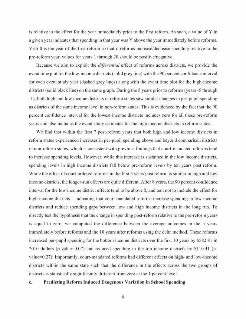
is relative to the effect for the year immediately prior to the first reform. As such, a value of Y in

a given year indicates that spending in that year was Y above the year immediately before reforms.

Year 0 is the year of the first reform so that if reforms increase/decrease spending relative to the

pre-reform year, values for years 1 through 20 should be positive/negative.

Because we aim to exploit the differential effect of reforms across districts, we provide the

event time plot for the low-income districts (solid grey line) with the 90 percent confidence interval

for each event study year (dashed grey lines) along with the event time plot for the high-income

districts (solid black line) on the same graph. During the 5 years prior to reforms (years -5 through

-1), both high and low income districts in reform states saw similar changes in per-pupil spending

as districts of the same income level in non-reform states. This is evidenced by the fact that the 90

percent confidence interval for the lowest income districts includes zero for all these pre-reform

years and also includes the event study estimates for the high income districts in reform states.

We find that within the first 7 post-reform years that both high and low income districts in

reform states experienced increases in per-pupil spending above and beyond comparison districts

in non-reform states, which is consistent with previous findings that court-mandated reforms tend

to increase spending levels. However, while this increase is sustained in the low income districts,

spending levels in high income districts fall below pre-reform levels by ten years post reform.

While the effect of court-ordered reforms in the first 5 years post reform is similar in high and low

income districts, the longer-run effects are quite different. After 8 years, the 90 percent confidence

interval for the low income district effects tend to be above 0, and tent not to include the effect for

high income districts – indicating that court-mandated reforms increase spending in low income

districts and reduce spending gaps between low and high income districts in the long run. To

directly test the hypothesis that the change in spending post-reform relative to the pre-reform years

is equal to zero, we computed the difference between the average outcomes in the 5 years

immediately before reforms and the 10 years after reforms using the delta method. These reforms

increased per-pupil spending for the bottom income districts over the first 10 years by $582.81 in

2010 dollars (p-value=0.07) and reduced spending in the top income districts by $110.41 (p-

value=0.27). Importantly, court-mandated reforms had different effects on high- and low-income

districts within the same state such that the difference in the effects across the two groups of

districts is statistically significantly different from zero at the 1 percent level.

c. Predicting Reform Induced Exogenous Variation in School Spending

8

Having described how court-mandated reforms affect school spending in different districts,

we detail how we use these patterns to predict reform-induced spending changes for each district

that are unrelated to other unobserved changes that might be correlated with both school spending

and adult outcomes. To outline the logic, consider the following example. Based on Figure 1, one

can predict that 10 years following reforms, on average, spending in the lowest income districts

will increase by $582.81 versus a $110.41 decrease for the highest income districts. This prediction

relies on the systematic differences in how different kinds of district are affected by court-ordered

reforms and does not rely on the particular experiences of any one single district. As pointed out

in Hoxby (2001), the effect of a reform on spending depends on the type of school funding formula

introduced by the reform. Accordingly, while this is a perfectly valid prediction, one can get an

even more precise prediction if one also incorporates information about the kind of funding

formula introduced by the court-ordered reform.

Doing an event study analysis for the imposition of school funding formulas that include a

spending limit (see Appendix D) we find that in the 10 years after the imposition of a spending

limit, on average, spending in the bottom income districts falls by $15.39 (p-value=0.94) and

spending for the top income districts falls by $535.91 (p-value<0.01). Assuming these effects are

additive, a more precise prediction is that a court-ordered reform that imposes a spending limit

will increase spending for the lowest income districts by 582.81-15.39=$576.42 and decrease

spending for the highest income districts by 110.41+535.91=$646.32.

This example above illustrates how one can predict the spending increase a district would

experience due to the passage of a court-ordered reform based solely on the type of funding

formula introduced by the reform and the income level of the district prior to the passage of the

reform. Importantly, this prediction is not based on the actual spending increases experienced by

a district, but is a prediction based on the experiences of all districts facing the same kind of reform

and with the same observable characteristics prior to the passage of reforms. Even though our

approach is more complicated than the simple example above, the underlying logic is the same.

There are two key differences between how we construct our predicted reform-induced

spending increases and the construction in the example above. The first key difference is that our

prediction of the reform-induced effect for districts in any state is based on data from all other

states (i.e., excluding data for that particular state). This is to ensure that any predicted district-

level reform effects are not driven by any unobserved district-level factors that determine

9

actualized spending and are also correlated with student outcomes. The second key difference is

that we not only use the imposition of a spending limit as our type of reform, but we use the four

key reform types described in Jackson, Johnson and Persico (2014) -- foundation plans, spending

limits, reward for effort plans, and equalization plans. Foundation plans guarantee a base level of

per-pupil school spending. Spending limits prohibit per-pupil spending levels above some

predetermined amount. Reward for effort plans match locally raised funds for education with

additional state funds (typically in low income districts). Equalization plans typically tax wealthier

districts and redistribute funds to low wealth districts. These four key reform types are not mutually

exclusive as many states’ implemented formula change involved more than one of these types.

More detailed descriptions of this typology of reforms and event study estimates for each formula

type on spending are presented in Appendix D. We construct out-of-sample district-specific

predicted reform-induced spending increases in three steps as described below.

Step 1: For each court-ordered reform we determine the funding formula type that the reform

introduced by associating any formula change within three years of a court order to that reform.

Step 2: Omitting data for the state for which the prediction is being created, we estimate the

dynamic treatment effect of a court order interacted with the formula type associated with that

reform for each district income group in 1962. We estimate [2] below where $dst is per-pupil

spending, sFI is an indicator for the type of funding formula introduced by the court order (more

than one formula type can be introduced by the same court-ordered reform), court

yI is an indicator

variable denoting year of the observation relative to the year of the first court-ordered reform for

that state (i.e., 5

courtI is equal to 1 if the observation is five years before the first court-ordered

reform and zero otherwise), and dQ is the quartile group of the district in the state distribution of

median income in 1962 (prior to any reforms). All other common variables are defined as in [1].

[2] , , 1972, ,$,$ $

s s

F Fcourt court court court

dst F d y F q y F d y F y d t dtI Q I I I

The coefficients , ,

court

F q ymap out the effect after y years of a court-ordered reform that introduced

formula F for a district in income percentile group q. To improve our ability to predict reform-

induced spending increases we also use 1972,$ d , the district’s per-pupil spending level relative to

the state average in 1972 (prior to the passage of reforms) to predict the marginal effect of any

10

reform. Accordingly, the coefficients ,$,

court

F ymap out the effect after y years of a court-ordered

reform that introduced formula F for a district with relative per-pupil spending level $ in 1972.

Step 3: Because reforms do not take full effect immediately, we use the average effect

between 3 and 8 years after reforms. As such, dSpend , our prediction of the spending change a

district will experience due to the passage of a court-ordered reform, is the estimated change in

spending between three and eight years after a court-mandated reform for similar districts (same

pre-reform relative income level, same pre-reform relative spending level) facing the same kinds

of formula changes (foundation, spending limit, reward for effort, equalization) in different states.

d. Creating an Instrument for School Spending

In predicting adult outcomes, our endogenous treatment variable is the natural log of average

school spending over the previous 12 years. This measures average school spending across all

school-age years (5 to 17) for expected high school graduates that year. Having predicted the

spending change a district will experience with the passage of a court order, we now show how

the interaction between this district-specific prediction, dSpend , and the timing of court-ordered

reforms isolates plausibly exogenous variation in school spending that is unrelated to potentially

confounding district-level determinants of school spending. We estimate equation [3] where

ln($ )dstis the natural log of average school spending over the previous 12 years, dSpend is our

scalar district-specific prediction of the reform-induced spending change, court

yI are flexible event

time indicators, d is a district fixed effect, t is a year fixed effect, and dt is random error.

[3] dttddt

court

yspend

court

yddst ZISpend ,)()$ln(

The coefficients Spend,

court

ymap out the spending change associated with a court-mandated reform

for a district that is predicted (based on similar districts in other states) to double school spending

by years 3 through 8 post reform. To show the changes in spending both by duration of exposure

and by predicted treatment intensity, Figure 2 plots the estimated flexible event study coefficients

for a 5 percent predicted change, a 10 percent change, and a 20 percent predicted change. If our

instrument has identified exogenous variation, districts that saw larger versus smaller predicted

spending increases due to reforms should be on very similar trajectories prior to reforms. Also, if

the instrument is valid, after reforms districts with larger versus smaller predicted spending

increases due to reforms should experience larger versus smaller actual spending increases.

11

To isolate spending changes associated with SFRs, we also include Zdt, controls for an array of

other policies that overlap our study period (Johnson, 2013; Chay, Guryan, & Mazumder, 2009;

Hoynes, Schanzenbach, & Almond, 2012). These include county-by-year measures of school

desegregation, hospital desegregation, community health centers, state funding for kindergarten,

per capita Head Start spending, Title I school funding, imposition of tax limit policies, and average

childhood spending on food stamps, Aid to Families with Dependent Children, Medicaid, and

unemployment insurance. Additionally, to remove any pre-trend differences between reform and

non-reform districts we also include linear trends for the poverty rate in the district in 1962, and

Census division-specific year fixed effects.

Because we interact each event-study year indicator with the relevant predicted spending

increase, the model imposes a linear relationship between predicted spending and actual spending

for each event-study year, but imposes no structure on the relationship between predicted spending

and actual spending over time. As such, the flexible model does not dictate that effects over time

for a predicted 10 percent increase have to be greater than that of a 5 percent increase, and the two

lines can even cross. We find districts predicted to experience 5, 10, and 20 percent spending

increases were on similar trajectories prior to reforms. One cannot reject the hypothesis of no

differential pre-trending at the 10 percent level consistent with our predicted spending changes

being exogenous. Despite similar pre-reform trajectories, these districts were on very different

trajectories of spending after reforms. All three groups see increased spending growth post reform

with the larger increases for districts with larger predicted effects. The F-statistic on the post-

reform year indicators yields an F-statistic over 50 (p<0.0000).

Figure 2 is a visual representation of our first stage that isolates exogenous variation in school

spending across cohorts within the same district. If there is a causal relationship between school

spending and adult outcomes, one should observe (a) no differential pre-reform trends in outcomes

for districts with larger or smaller predicted reform-induced spending increases, and (b) larger

improvements in outcomes for post-reform cohorts in districts with larger predicted reform-

induced spending increases. These are the patterns we document in Section V.

III. Description of the Longer-Run Outcome Data

Our data on longer-run outcomes come from the Panel Study of Income Dynamics (1968–

12

2011) that links individuals to their census blocks during childhood.11 Our sample consists of PSID

sample members born between 1955 and 1985 who have been followed from 1968 into adulthood

through 2011. This corresponds to cohorts that both straddle the first set of court- mandated SFRs

(the first of which was in 1972) and who are also old enough to have completed formal schooling

by 2011. Two thirds of those in these cohorts in the PSID grew up in a school district that was

subject to a court-mandated school finance reform between 1972 and 2000. We include both the

Survey Research Center component and the Survey of Economic Opportunity component,

commonly known as the “poverty sample,” of the PSID sample. Parental income and education

variables are averaged over the ages of 12 and 17, and family structure is measured at birth.

Following Ben-Shalom, Moffitt, and Scholz (2011) and Short and Smeeding (2012), a child is

defined as “low income” if parental family income falls below two times the poverty line for any

year during childhood.12 This captures both the poor and the near poor. Due to the oversampling

of poor families, 59 percent of the sample were low income as children. Henceforth, children from

families who were not low income (as defined above) will be referred to as “non-poor”.

We match childhood residential location address histories to the school district boundaries

that prevailed in 1969 to avoid complications arising from endogenously changing district

boundaries over time. We use the earliest available address in childhood to circumvent concerns

of endogenous mobility. The algorithm is outlined in Appendix E.13 We show that our results are

robust to using only those who lived in their childhood residence prior to initial court orders. Each

record is merged with data on school spending and the aforementioned school finance variables at

the school district level that correspond with the prevailing levels during their school-age years.

Finally, we merge in county characteristics from the 1962 Census of Governments, and

information on the key policy changes (described in Section II) during childhood, allowing for an

11 The PSID began interviewing a national probability sample of families in 1968. These families were re-interviewed each year through 1997, when interviewing became biennial. All persons in PSID families in 1968 have the PSID “gene,” which means that they are followed in subsequent waves. When children with the “gene” become adults and leave their parents’ homes, they become their own PSID “family unit” and are interviewed in each wave. The original geographic cluster design of the PSID enables comparisons in adulthood of childhood neighbors who have been followed over the life course. Studies have concluded that the PSID sample remains representative of the national sample of adults (Gottschalk et al., 1999; Becketti et al., 1997).12 The poverty line is defined by family composition, such that children are defined as “low income” if the family’s income-to-needs ratio falls below two for any year during childhood.13 Many school districts were counties during this period, including more than one-half of Southern school districts.

13

unusually rich set of controls.14

The final sample includes 93,022 adult person-year observations of 15,353 individuals

(9,035 low-income children; 6,318 non-poor children) from 1,409 school districts, 1,031 counties,

and all 50 states and the District of Columbia.15 Because we use individuals born between 1955

and 1985, the oldest cohort is observed at age 56, while other cohorts are observed at age 30. To

compare individuals from different cohorts at similar ages, we focus on adult observations between

the ages of 25 and 45. The mean age is 32.9 years for economic outcomes. The set of adult

outcomes examined include (a) educational outcomes—whether graduated from high school, years

of completed education (at the most recent survey) – and (b) labor market and economic status

outcomes (measured annually and expressed in 2000 dollars)—wages, family income, and annual

incidence of poverty in adulthood (ages 25–45). All analyses include men and women with

controls for gender. Summary statistics are presented in Table 1.

Average years of education is 13.18, where children from low-income families have about

1 fewer years of schooling than non-poor children. We examine wages (annual earnings/annual

work hours) as our main labor market outcome. We use wages only for those who have positive

earnings in a given year. However, because we have multiple adult observations for each

individual, we have valid wage observations for about 95 percent of the sample. This is more than

datasets such as the CPS or the Census that only have earnings at a single point in time (about two-

thirds of individuals). This feature of the data allows us to better detect effects for those with low

labor market attachment. The average wage in 2000 dollars at age 30 for those from low-income

families is $10.60 and that for those from non-poor families is about 28 percent higher at $13.60.

IV. Empirical Strategy for Estimating Effects on Adult Outcomes

We aim to explore how exogenous changes in school spending induced by SFRs affect

adult outcomes. Our emphasis on using only exogenous variation is motivated by the observation

14 The data we use include measures from 1968–1988 Office of Civil Rights (OCR) data; 1960, 1970, 1980, and 1990 Census data; 1962–1999 Census of Governments (COG) data; Common Core Data (CCD) compiled by the National Center for Education Statistics; Regional Economic Information System (REIS) data; a comprehensive case inventory of court litigation regarding school desegregation over the 1955–1990 period (American Communities Project); and the American Hospital Association’s Annual Survey of Hospitals (1946–1990) and the Centers for Medicare and Medicaid Services data files (dating back to the 1960s) to identify the precise date in which a Medicare-certified hospital was established in each county of the U.S. (an accurate marker for hospital desegregation compliance).15 The average school district has 11 PSID sample children; half of the districts have at least 9 PSID sample children; less than 6% of school districts have only one PSID sample child; and one quarter have at least 25 PSID children.

14

that simply comparing outcomes of students exposed to more or less school spending, even within

the same district, could lead to biased estimates of the effect of school spending if there were other

factors that affect both outcomes and school spending simultaneously. For example, a decline in

the local economy could depress school spending (through home prices or tax rates) and also have

deleterious effects on student outcomes through mechanisms unrelated to school spending such as

parental income. This would result in a spurious positive correlation between per-pupil spending

and child outcomes. Conversely, an inflow of low-income, special needs, or English language

learner students could lead to an inflow of compensatory federal funding while simultaneously

generating reduced student outcomes. This would lead to a spurious negative relationship between

spending and student outcomes.

To highlight this point, we test the exogeneity of school spending. First, we predict both

high school graduation and adult wages (at age 30) using the fitted values of a regression of these

outcomes on parental income, race, mother’s and father’s education and occupational prestige

index, mother’s marital status at birth, birth weight, childhood county-level average per-capita

expenditures on Head Start, AFDC, Medicaid, and food stamps during school-age years—this is

an effect-size weighted index of childhood family/community factors. We then examine whether

predicted outcomes are related to the average actualized district per-pupil spending during ages 5-

17. The results are presented in the top panel of Table 2. Naïve OLS models that rely on variation

in school spending both within and across states (Top panel, columns 1 and 2) show a strong

positive and statistically significant association between school spending and predicted outcomes.

This is consistent with most people’s priors that raw correlations between spending and outcomes

are likely to be positively biased because areas with higher levels of school spending (in the cross

section) will tend to comprise children from more advantaged family backgrounds in both

observed and unobserved ways. However, when we examine the relationship between changes in

actualized spending within districts over time and changes in predicted outcomes (columns 3 and

4), there is a statistically significant negative relationship for predicted high school completion and

a marginally statistically significant negative relationship for wages at age 30. This is consistent

with there being a negative bias when using actualized spending changes within districts over time

to predict better outcomes. We also look at the relationship between school inputs (student-teacher

ratios) and endogenous changes in school spending (Column 5). Surprisingly, while the point

estimates show the expected sign, endogenous spending changes are not significantly related to

15

observable school resource inputs.

To provide a basis for comparison, we instrument for school spending with the predicted

spending increase interacted with indicators for each year of school-age exposure to reforms (0 to

12). In contrast to the OLS estimates, our exogenous school spending changes (based on the timing

and type of SFRs) are not related to changes in predicted outcomes, and the effects go in different

directions for the two predicted outcomes (lower panel). Looking to the student-teacher ratio,

however, reveals a stark difference between the OLS variation and the 2SLS/IV identifying

variation; exogenous spending increases are associated with large statistically significant

reductions in the student-teacher ratio. Table 2 illustrates that OLS estimates of the effects of

school spending on outcomes may be negatively biased, and may not be associated with improved

school inputs. In contrast, the exogenous variation in spending due only to SFRs is likely to

uncover the true causal relationship as mediated by improved school inputs. We show evidence of

this in Sections V and VI.

a. The Effect of Predicted Spending Increases on Actual Spending Increases

Our treatment measure of exposure to school spending is ln(PPE5-17), the natural log of

average per-pupil spending in an individual’s birth district during the years when that individual

was ages 5 through 17 (school age years). A 0.1 increase of this average can be interpreted as a 10

percent increase in per-pupil spending for all 12 years of an individual’s school career.16 To show

consistency across the CCD universe of school districts and the sample of districts covered in the

PSID, we begin by presenting “first-stage” event study model [4] estimates on average per-pupil

spending using our PSID sample (Figure 3). The model includes the same set of control variables

as that used in the CCD with the addition of controls for individual characteristics.17

Figure 3 presents the estimated event-study effects on average actual spending during ages

5-17 associated with a predicted 5, 10, and 15 percent spending increase between three and eight

years after a court-mandated reform. Event study year zero on the x-axis is the year an individual

turns 17 minus the initial year of a court-ordered reform (negative values indicate pre-reform

cohorts). The average predicted spending change is 5 percent, the standard deviation of the

16 We express spending in logs because school spending likely exhibits diminishing marginal returns. The patterns of results are very similar when spending is expressed in levels (See Appendix F).17 The individual level controls include race, race-by-census division of birth year fixed effects, and controls for parental education and occupational status, parental income, mother’s marital status at birth, birth weight, child health insurance coverage, and gender. Results are similar without these controls.

16

predicted spending change is roughly 9 percent, and one-quarter of districts in reform states had

predicted spending increases of more than 10 percent. The results mirror the patterns using the full

universe of public school districts (Figure 2) -- supporting the generalizability of the PSID results

for cohorts born between 1955 and 1985. As in the CCD data, districts with larger versus smaller

predicted spending increases due to reforms were on similar trajectories in spending prior to

reforms; however, after reforms districts with larger predicted spending increases due to reforms

experienced larger actual spending increases. These patterns are the same for both low-income

and non-poor children. The right figure presents the event study for a 10 percent predicted spending

increase along with the 90 percent confidence interval. We will show this same figure for all long-

run outcomes, so it is important to note that a 10 percent predicted increase during years 3 and 8

post reform corresponds to about a 15 percent increase in actual school-age spending for fully

exposed cohorts (all 12 years).

The reform-induced increases in average school spending during ages 5-17 are small in the

first three years following reforms, but increase roughly linearly with school-age exposure years

4 through 12, and event-study years 13 through 17, before flattening out. The estimated pattern is

insensitive to whether a balanced or unbalanced panel is used. Figure 3 is a visual representation

of our first stage that isolates exogenous variation in school spending across cohorts within the

same district. We now discuss the patterns one should observe for outcomes if there is a causal

effect of these increases in school spending on outcomes.

b. Hypothesized Effects of Reform Induced Spending Increases On Adult Outcomes

Figures 2 and 3 show two distinct sources of variation in school spending during one’s

school-age years: (a) the staggered timing of court-mandated SFRs across districts to implement a

cohort level “event-study” analysis (variation in the timing of reforms across cohorts), and (b) the

fact that the same reform led to different changes in spending across districts (variation in intensity

among exposed cohorts). Accordingly, there are two natural tests of whether reform-induced

spending changes have a causal effect on adult outcomes. The first test is whether exposed cohorts

from those districts that experienced increases in per-pupil school spending also had improved

outcomes relative to unexposed cohorts from the same district. The second test is whether the

improvements observed for exposed cohorts (relative to unexposed cohorts) are larger for those

from districts that experienced larger increases in per-pupil school spending. Because not all

cohorts within a district are equally treated (some are exposed to spending increases for more of

17

their school-age years than others), and not all districts experience the same changes in spending

after reforms (some districts experience larger spending increases than others), both of these tests

can be implemented within a single event-study framework. We lay out the cross-cohort and cross-

district patterns in outcomes one should observe in an event-study analysis if there is a causal effect

of increased spending due to reforms on adult outcomes.

If there is a causal effect of school spending on outcomes, and there are no pre-existing

cohort trend differences across districts that experience increases in spending, then an event-time

figure across cohorts for a given increase in school spending should follow patterns similar to the

stylized patterns presented in Figure 4. The X-axis is years of exposure to the reform for a given

cohort, and the y-axis is the cohort-level mean of some outcome for which higher values are better.

For those cohorts who were 18 or older at the time of the passage of reforms (to the left of

0), there should be no systematic increase or decrease in the outcome across cohorts because none

of these cohorts was exposed to reforms. As such, an event-study graph of outcomes by cohorts

should be relatively flat across cohorts that were too old to be affected by the reforms. Also,

outcomes should be similar across the pre-reform cohorts across districts that experienced large

and small increases in school spending after reforms. For those cohorts who were of school-going

age when reforms were implemented (i.e. between the ages of 17 and 5, indicated by relative years

0 to 12 on the x-axis), outcomes should both be better than those for the unexposed cohorts and

increasing in the number of years of exposure. That is, for a given increase in spending, relative to

unexposed cohorts, cohorts exposed to increased spending for a longer period of time should have

larger improvements (variation in timing). Additionally, for a given duration of exposure, relative

to unexposed cohorts, individuals exposed to larger spending increases should have larger

improvements in outcomes than those from districts with smaller increases in spending (variation

in intensity). As such, among those exposed, the relationship between years of exposure and good

outcomes should be positive, and this relationship should be more positive for districts that

experience larger increases in spending. This is depicted in the two upward sloping segments for

the partially exposed cohorts, where the dashed line is steeper for larger increases in spending.

Among more recent cohorts (i.e., those who were younger than 5 or unborn at the passage

of reforms) all 12 of their school-age years were post-reform, and as a result, we hypothesize these

cohorts should have better outcomes than the partially exposed cohorts. Spending increases

continued beyond 12 years post reform (see Figures 2 and 3); thus, among the fully treated cohorts,

18

recent cohorts may have better outcomes than older cohorts (because more recent cohorts will have

experienced more total spending during their school-age years). As with the partially exposed

cohorts, one might expect better outcomes (relative to untreated cohorts) for the fully treated

cohorts from high-increase spending districts than low-increase spending districts. Note that

because those with fewer years of exposure also experience reforms when they are older, we cannot

disentangle years of exposure from the effect of age of exposure.

In sum, if there is a causal effect of spending on outcomes and the spending increases due

to reforms are exogenous to changes in outcomes, then the event-study plot of outcomes for

districts that experience small and large spending increases due to reforms should follow the

stylized patterns in Figure 4. That is, outcomes should be improving in years of exposure to reforms

(time variation) and the relative improvements should be larger in districts with larger increases in

school spending (variation in intensity). We present such patterns below.

c. Analyzing the Effect of Reform Induced Spending Increases on Adult Outcomes

We test for the patterns hypothesized in Figure 4 across several adult outcomes. Our

measure of treatment intensity for each district is the predicted reform-induced spending change (

dSpend ), which is based on the predicted change in spending between three and eight years after

a court-mandated reform for similar districts (same pre-reform relative income level, same pre-

reform relative spending level) facing the same kinds of formula change (foundation, spending

limit, reward for effort, equalization) in different states (as described in Section II). The event-

study models used to analyze the effect of predicted school spending changes on the difference in

outcomes between treated and untreated cohorts involve estimating equations of the form [4]:18

(4)

idb

r

g

r

bdddbidb

Tt

ddidbTt

Tt

ddidbTtd

Tt

didbTtidb

bbWZXSPENDTtTt

SPENDTtTtSPENDTtTtY

*)(1

11

1960

20

13

*

12

0

*2

20

*

where i indexes the individual, d the school district, b the year of birth, g the census division of

birth, and r the racial group. The term d represents a vector of school district fixed effects, and

dSPEND is the predicted SFR-induced change in per-pupil spending in district d. The flexible

timing indicators, TtTt didb

*1 , equal 1 if the year the individual from school district d turned

18 This approach is similar to Johnson (2011) in a study of the long-run effects of court-ordered school desegregation.

19

age 17 (tidb) minus the year of the initial SFR court order in school district d ( *

dT ) equals a value

between -20 and 20. For example, values for *

didb Tt between -20 and -2 represent pre-treatment

years; a value of -1 represents an individual who was 18 when court-mandated SFR was first

enacted and thus was not exposed, which is used as the reference group category; values between

0 and 12 represent school-age years of SFR exposure; and values greater than 12 represent persons

who were younger than 5 when reforms were enacted. The event-study year (t - T) is 0 when the

year in which an individual was age 17 (typically, a high-school senior) equals the initial year of

court-mandated SFR for the school district in which the person grew up.

The variables of interest are the coefficients on the interactions between dSpend and the

flexible event-time indicators. These estimates illustrate the exact timing of changes in outcomes

in relation to the number of school-age years of exposure to SFR and the predicted changes in

spending. These coefficients map out the difference in outcomes between exposed and unexposed

cohorts from districts with larger versus smaller predicted reform-induced spending increases.

Equation [4] provides a flexible description of the subsequent adult attainment outcomes in relation

to the cohort- and district-specific timing of reform-induced changes in school spending.

The validity of our empirical design relies on the assumption that districts that experienced

increases in school spending due to reforms were not already on a differential trajectory of

improving outcomes. As such, we also present the flexible time indicators interacted with the

increase in spending for years prior to reforms. A plot of the estimates of the pre-reform indicator

time dummies interacted with SPENDd, will show if outcomes in districts with larger or smaller

spending increases were on a different trajectory than non-reform districts prior to enactment of

reforms. This provides a test of exogeneity of the timing and scope of initial court orders.

This model can be viewed as a triple-difference strategy that compares the difference in

outcomes between cohorts within the same district exposed to reforms for different amounts of

time (variation in exposure) across districts with larger or smaller changes in school spending due

to reforms (variation in intensity). To ensure that it isolates exogenous changes due to reforms we

include a variety of additional controls. The model includes school district fixed effects ( d ), race-

specific birth year fixed effects ( ), race-by-region of birth cohort trends ( ), and controls

for an extensive set of child and childhood family characteristics ( idbX : parental education and

occupational status, parental income, mother’s marital status at birth, birth weight, child health

r

b br

g *

20

insurance coverage, and gender). To control for trends in factors hypothesized to influence the

timing of SFR, we also included interactions between 1960 characteristics of the county of birth

and linear trends in the year of birth ( bW d1960 ): 1960 county poverty rate, percent black, average

education level, percent urban, and population size. Finally, to account for the effect of other

policies, we include county-by-birth year level measures of school desegregation, hospital

desegregation, community health centers, state funding for kindergarten, imposition of tax limit

policies, in addition to per capita expenditures on Head Start (at age four), Title I school funding

(average during ages 5-17), and average childhood spending on food stamps, Aid to Families with

Dependent Children (AFDC), Medicaid, and unemployment insurance, ( ). Few studies

simultaneously account for so comprehensive a set of policies. Standard errors are all clustered at

the school district level.

One potential parental response to existing school quality differences across public schools

is to move to a different location or enroll children in a private school.19 To avoid bias due to

endogenous mobility, we identified the county and school of upbringing based only on the earliest

childhood address.20 This captures the quality of the public schools potentially attended instead of

the quality of schools and classes actually attended. As such, one can interpret our results as

providing “intent to treat” estimates of the effects of school spending.21

To present both the time and intensity variation on the same graph, we display the effects

for both a 15 and 20 percent school spending increase. That is, we plot the coefficients for the

flexible event time figures interacted with dSPEND where dSPEND is set to 0.05 and 0.1,

respectively. The event study figures provide a visual depiction of the reduced-form effect of court-

ordered reforms on outcomes. To provide point estimates and statistical inference tests for the

effect of spending on outcomes, we employ 2SLS/IV regression analysis.

c. Estimating of the Causal Effect of School Spending on Adult Outcomes

To identify effects of school spending solely from the exogenous variation in school

spending caused by reforms, we use the number of school-age years of exposure interacted with

19 After SFRs in California, the share of students attending private schools rose about 50 percent (Downes & Schoeman, 1998), and educational foundations grew tremendously (Brunner & Sonstelie, 2003). Privatization grew disproportionately in districts constrained by the SFR formula to spend less than they traditionally had.20 Because we use the earliest address available for children, limiting the analysis sample to those who lived at that childhood residence prior to initial court orders reduces the sample by less than 5 percent. Results are similar when the sample is restricted to individuals who lived in their childhood residence prior to the initial court orders. 21 We recognize that school spending varies within districts. However, these data are not typically reported.

cbZ

21

the district-specific predicted change in spending as our exogenous instrument for school spending.

Specifically, we estimate the following system of equations by two-stage least squares (2SLS).

[5] *

5 17 idb 1 2 3 1960 1 1 1ˆln( ) * *r r

idb d d idb db d d b gPPE t T SPEND X Z W b b

[6] 5 17 idb 1960ˆln( ) ( ) *r r

idb idb db d d b g idbY PPE X Z W b b

All variables are defined as in [4] and the same controls are included. The difference between [4]

and [5] and [6] is that we replace the event time indicators interacted with predicted spending

changes in [4] with a single measure of per-pupil spending, ln(PPE5-17)idb, in the second stage

regression in [6]. We instrument for ln(PPE5-17)idb, with the event time indicators (i.e., an indicator

for each year of exposure between 0 and 12 years) interacted with the district-specific predicted

spending change, ddidb SPENDTt * . Standard errors are clustered at the school district level.

The instrumental variables models exploit both the exogenous variation in timing and

intensity of school spending changes due to court-mandated reforms. The coefficient from [6]

should uncover the causal effect of school spending on outcomes so long as the timing of court

mandated SFRs is exogenous to changes in outcomes across birth cohorts within districts that saw

larger versus smaller predicted increases in school spending due to the reforms. Both the event-

study analyses and additional placebo tests suggest that this is the case.

V. Effects on Longer-Run Outcomes

Educational Attainment. Figure 5 presents the semi-parametric event-study model results

of the effects of reform-induced changes in per-pupil spending on years of completed education.

On the left we present the coefficients on the individual event time indicator variables interacted

with the district-specific change in spending for a 5 percent and 10 percent predicted spending

increase. Note, these are reduced-form effects of predicted spending increases, not effects of actual

spending increases (estimates of actual spending are provided in the 2SLS regression results). Even

though [4] imposes a linear relationship between dSpend and outcomes in any given year, the

relationship between dSpend and outcomes varies across years (e.g., larger spending increases

can improve outcomes for those with 8 years of exposure but hurt outcomes for those with 9 years

of exposure). As such, the estimated trajectories across time for different spending levels may not

be parallel, and can even cross. Insofar as the model shows better outcomes for treated cohorts in

districts with larger spending increases, this is an artifact of the data and is indicative of causal

22

effects (rather than an artifact of any modeling assumption). If there are true causal effects, one

would expect these lines to possibly cross and be centered on zero during pre-treatment years, but

would expect the effect to be increasing with duration of exposure and be consistently larger for a

10 percent increase than a 5 percent increase (with no causal effect, both lines will be centered on

zero so that there will be no tendency for one line to be systematically higher than the other). The

reference cohort (year 0) are individuals who were 17 years old when the court order was first

enacted. The right panel shows the effect of a 10 percent predicted spending increase along with

the 90 percent confidence interval for each event study year.

Overall, one can see clear patterns of improved outcomes for exposed cohorts in districts

with larger predicted spending increases. Districts that saw increases in school spending exhibit

no discernible trending in educational attainment for the pre-treatment cohorts (those that were 18

or older at the time of the reforms). Importantly, the pre-reform year effects are very similar for

districts with a predicted 5 and 10 percent spending increase (these lines often cross for the pre-

reform cohorts). This indicates that the timing of the reforms was likely exogenous to changes in

educational attainment in a given district and that the size of the predicted spending increase was

unrelated to the pre-reform trends in outcomes. This lends credibility to our research design and

the resulting 2SLS estimates. Looking at treated cohorts, the results are consistent with significant

causal effects on exposed cohorts. That is, cohorts with more years of exposure to predicted

spending increases have higher completed years of education than unexposed cohorts and cohorts

with fewer years of exposure. Also, the increases associated with exposure are larger in districts

with the larger predicted increases in spending (indicated by the line for a 10 percent increase

being consistently above that of a 5 percent increase for the exposed cohorts). Both the patterns in

timing and intensity support the hypothesis that policy-induced increases in school spending led

to significant increases in educational attainment. The panel on the right only depicts the event

time estimates for a 10 percent predicted increase along with the 90 percent confidence interval

for each event study year. About one quarter of districts have predicted spending increases at least

this large. The panel on the right shows the same pattern of results as the left, however one can see

that each event-study year estimate is noisy. Having said this, after 9 years of exposure, one can

reject the null hypothesis that most of the post-reform years is different from that of no exposure

at the 10 percent level. Note that testing the difference between individual years of exposure is low

powered, and is not a test of the broader hypothesis that variation in school spending is related to

23

variation in outcomes. To test this broader hypothesis we rely on the 2SLS regressions that impose

a bit more structure on the data.

Because residential mobility across counties and private school attendance are more

common among affluent families than low-income families, one might expect larger effects among

low income children.22 Furthermore, prior research has shown that children from low-income

families may be more sensitive to changes in school quality and school-related interventions than

children from more advantaged backgrounds.23 For these reasons, we also conduct all analyses

separately by childhood economic status (low income vs non-poor) in Figure 6.24 Event study

figures for a 10 percent predicted increase and the 90 percent confidence intervals are shown

separately for low-income (left) and non-poor (right) children. For low income children, the event-

study plots follow the same pattern as for the overall sample, but the difference between the

exposed and unexposed cohorts are more pronounced. In contrast, the estimates for non-poor

children are much weaker. For non-poor children, there is suggestive evidence of an increase in

educational attainment after the passage of reforms. Exposed cohorts do appear to have higher

years of education (e.g., increases in event study years 4-11) than the pre-reform cohorts, and

districts that experienced larger predicted spending increases do tend to have better educational

attainment than those with smaller predicted spending increases for the exposed cohorts. The

pattern of results suggest small effects for children from non-poor families and large effects for

low-income children.

To examine what margin of educational attainment was most affected, we turn to the

probability of high school graduation. The results for high school completion reveal very similar

patterns to those for years of education. Figure 7 presents the event study plots for the effects of a

10 percent predicted spending increase on the likelihood of high school graduation for children

from low-income (left) and non-poor families (right). As with completed years of education, there

is no trending in outcomes for the pre-reform cohorts. However, for low income children, the

likelihood of high school graduation is increasing in years of exposure for exposed cohorts. For

non-poor families, there is no visible systematic effect on high school graduation.

22 Prior research shows that while residential instability is greater for poor families, poor families are far less likely to move to better neighborhoods, and are less responsive to policy changes due to the greater residential location constraints they face (Johnson, 2008; Kunz, Solon et al., 2008; Mare et al., 2008).23 E.g., Krueger and Whitmore (2001).24 In pooled models we include childhood economic status indicator interactions with all control variables and test for differential spending effects.

24

The consistent pattern of these results indicate that these effects reflect the causal effect of

school spending particularly for children from low-income families. That is, we see that (a)

increases in educational outcomes occur only for children exposed during school-age years, (b)

improvements are monotonically increasing with years of exposure, (c) improvements are greater

with larger exogenously predicted spending increases, (d) the timing of improved outcomes track

the timing of increased spending, and (e) there are no differential pre-reform trends in outcomes

for districts with larger or smaller predicted spending increases. These patterns are all more

pronounced for children from low-income families.

Having established visually that there are significant policy-induced improvements in long-

run educational attainment associated with larger exogenous predicted school spending increases

for exposed cohorts, we now quantify the causal relationship between actual school spending and

longer-run educational attainment. For this we turn to the instrumental variable models that use

the event study patterns to predict changes in childhood exposure to per-pupil spending. Putting

all the variation together, the 2SLS/IV models provide a direct estimate of the effect of school

spending on adult outcomes and allow for tests of statistical significance.

The regression estimates are presented in Table 3. The main outcomes are the educational

attainment measures and the variable of interest is the natural log of average per-pupil spending

during an individual’s school-age years. The interpretation of a 0.10 and 0.2 change in this variable

is the effect of increasing school spending by 10 and 20 percent throughout all 12 of an individual’s

school-age years, respectively. The excluded instruments for this spending variable are indicators

for each number of school-age-years of exposure to reforms (0 to 12) interacted with the school

district’s reform-induced change in school spending. The first stage F-statistic is greater than 10

in all models. For comparison purposes, we also show estimates from ordinary least squares (OLS)

regression models that do not account for the possible endogeneity of school spending.

Column 2 of Table 3 presents the 2SLS/IV regression results based on variation presented

in Figures 12 for all children. The 2SLS estimates indicate that increasing per-pupil spending by

10 percent in all 12 school-age years increases educational attainment by 0.27 years on average

among all children. Results from column 3 show even larger effects for low-income children. For

children from low-income families, increasing per-pupil spending by 10 percent in all 12 school-

age years increases educational attainment by 0.44 years. This estimate is statistically significant

at the 5 percent level. In contrast, for non-poor children, a 10 percent increase in per-pupil spending

25

throughout one’s school-age years increases educational attainment by only 0.075 years and this

estimate is not statistically significant. To put these educational attainment estimates in

perspective, the education gap between children from low-income and non-poor families is one

full year. Thus, the estimated effect of a 22.7 percent increase in per-pupil spending throughout all

12 school-age years for low-income children is large enough to eliminate the education gap

between children from low-income and non-poor families. In relation to current spending levels

(the average for 2012 was $12,600 per pupil), this would correspond to increasing per-pupil

spending permanently by roughly $2,863 per student.

Columns 5 and 6 present the 2SLS regression estimates for the likelihood of high school

graduation. Overall, the 2SLS estimate indicates that increasing per-pupil spending by 10 percent

in all 12 school-age years increases the probability of high school graduation by 9.5 percentage

points. The 2SLS estimate indicates that increasing per-pupil spending by 10 percent in all 12

school-age years increases the probability of high school graduation by 11.6 percentage points (p-

value<0.01) for low income children and 6 percentage points (p-value<0.10) for non-poor

children. The 95 percent confidence interval for the effect of a 10 percent increase for low-income

children is between 3.3 and 20.5 percentage points. The high school graduation rates for low-

income and non-poor children were 79 and 92 percent, respectively. Accordingly, increasing per-

pupil school spending by 10 percent over the entire schooling career of a cohort of low-income

children will increase the high school graduation rate for those children by between 4 and 26

percent. These results suggest some weak positive effects for more affluent children and large

positive effects for low income children.

To put these estimates in perspective, attending Head Start or the Perry Pre-School

Program increased high school completion by 8.5 and 14 percentage points, respectively (Carneiro

and Heckman 2003; Deming 2009). Also, Barrow, Claessens, and Schanzenbach (2013) and

Schwartz, Stiefel and Wiswall (2013) find that attending small schools increases graduation rates

for low-income children by between 16 and 18 percentage points. Accordingly, our effects on

educational attainment are in line with those of other successful interventions.

In sum, both the event study and 2SLS/IV models reveal that exogenous increases in school

spending (caused by SFRs) led to substantial improvements in educational outcomes of affected

children. Both analyses suggest that there are much larger effects of school spending on

educational attainment of children from low-income families.

26

Labor Market Outcomes, Adult Family Income, and Poverty Status. The next series of

results reveal meaningful effects of school spending on low-income children’s subsequent adult

economic status and labor market outcomes, using the same model specifications. It is important

to note that our models that analyze economic outcomes (such as wages and annual family income)

use all available person-year observations for ages 20-45 and control for a cubic in age to avoid

confounding life cycle and birth cohort effects. Figures 9, 10, and 11 present event study school

spending effects on adult economic outcomes (ages 25–45), including wages (Figures 9), annual

family income (Figure 10), and the annual incidence of poverty (Figure 11), by childhood

economic status. In light of the parallel set of findings across all of these long-run economic

outcomes, the results are discussed in succession below. As with the educational outcomes, the

economic outcome patterns are similar to those hypothesized in Figure 4 for low-income children

and are indicative of the causal effects of increases in school spending induced by reforms.

We first discuss the effects on adult wages for the full sample (Figure 8). Overall, one can

see clear patterns of improved outcomes for exposed cohorts in districts with larger predicted

spending increases. Districts that saw increases in school spending exhibit no discernible trending

in wages for the pre-treatment cohorts and the pre-reform year effects are very similar for districts

with a predicted 5 and 10 percent spending increase. As before, these are reduced-form effects of

predicted spending increases, not effects of actual spending increases (estimates of actual spending

are provided in the 2SLS regression results). Looking at treated cohorts, cohorts with more years

of exposure to predicted spending increases have higher wages than unexposed cohorts and cohorts

with fewer years of exposure. While not as pronounced as in the education outcomes, the increases

associated with exposure are larger in districts with the larger predicted increases in spending

(indicated by the line for a 10 percent predicted increase being consistently above that of a 5

percent increase for the exposed cohorts). The panel on the right depicts the event time estimates

for a 10 percent predicted increase along with the 90 percent confidence interval for each event

study year. The panel on the right shows the same pattern of results as the left. After 9 years of

exposure, one can reject the null hypothesis that most of the post-reform years is different from

that of no exposure at the 10 percent level. We now look at patterns for low-income and non-poor

families separately.

For both the log of wages and family income (Figures 9 and 11), there is no evidence of

trend differences prior to reforms between districts that saw larger or smaller increases in school

27

spending after reforms. In contrast, for children from low-income families, both wages and family

income exhibit substantial improvements across cohorts associated with more years of exposure

to a predicted spending increase. For children from low-income families, the increases are only

associated with the school-age years, and there is no systematic difference in outcomes across

cohorts born at different times but with the same number of years of exposure – consistent with a

causal effect of spending increases for children from low-income families. The results on wages

and adult family income for children from low-income families mirror those of the education

results. For children from non-poor families, there is suggestive evidence of small positive effects

on wages and annual family income in adulthood.

The 2SLS/IV estimates for adult economic outcomes are presented in Table 4. As shown

in Column 3, the 2SLS/IV estimates reveal that, for children from low-income families, increasing

per-pupil spending by 10 percent in all 12 school-age years increases adult wages by 9.5 percent.

This implies an elasticity of wages with respect to per-pupil spending close to 1. However, the 95

percent confidence interval of this estimate supports a range of elasticities between a modest 0.08

and a sizable 1.8. In contrast, the 2SLS estimate for children from non-poor families is much

smaller and statistically insignificant. It is worth noting that the point estimate implies that for non-

poor children, increasing per-pupil spending by 10 percent in all 12 school-age years increases

adult wages by 4.3 percent. While this effect is not statistically significant, the effect is

economically important and is suggestive of benefits for all children, with larger effects for those

from low income families.

While some of these wage effects will be due to increased years of schooling (for those

induced to stay in school longer), the effect of improved school quality on those who do not change

their school-going behaviors will be reflected in their wages but not their years of schooling.25 To

put our estimates in context, it is helpful to determine how much of the estimated effect on wages

can plausibly be attributed only to increases in years of schooling. Tables 3 and 4 indicate that

increasing school spending by 10 percent for all of a low-income child’s school-age years will

increase their years of schooling by 0.43 years and their adult wages by 9.5 percent. Recent

25 Recent studies find that improvement in instruction are reflected in improved outcomes above and beyond their effects on years of schooling. Goodman (2012) who finds that an addition year of math coursework in high school increases the earnings of Black males by 5 to 9 percent, even when one conditions on the overall years of schooling. Also, Vestman et al (2013) find that the effects of class size on earnings are much larger than imputed effects based on increases in years of education.

28

credible estimates of the returns to an additional year of schooling indicate returns between 9 and

28 percent26, so that wage effects between 3.87 and 12.04 percent can be expected only through a

years of schooling effect. The actual increase in wages of 9.5 percent is well within this range.

Because years of education may only capture some of the effect on wages, our estimates are

consistent with effect sizes suggested by the existing literature.

Note that while we look at individuals in their 40s, recent studies of interventions on

earnings tend to look at individuals in their 20s (e.g., Chetty et al, 2013). The estimated effects on

wages for those in their twenties likely understates the effect on permanent income. To assess the

importance of this, we estimate the effect of school spending interacted with a cubic in an

individual’s age. The implied age profile of the school spending effects on wages are presented in

Figure 10. One can reject the null of no age profile at the 5 percent level. The results imply that

the increase in wages that result from a 10% increase in school spending throughout the school-

age years is 2.8% at age 20, about 8% during one’s 30s, and 13.4% at age 45. Another important

aspect of our data is that we observe the same individuals in multiple years rather than at one point

in time (as in the CPS or Census). As such, individuals with low labor market attachment (who

might be highly responsive to improvements in school quality) who might not have earnings in

any given year can be observed with earnings in the PSID at some point over the panel, which

minimizes potential sample selection bias. To show the importance of this, we estimate wage

effects using only wage outcomes from the 2001 or 2011 waves (Table 5). Using a single year of

wage data yields point estimates between half and two-thirds as large as those using all years, and

yields standard errors four times as large. Haider and Solon (2006) show that using a single year

of data, and data at young ages, will lead one to understate effects on earnings. This appears to be

an important reason why our wage estimates are somewhat larger than others in the literature.

The 2SLS/IV estimates for the adult family income are similar to those of other outcomes.

As shown in the middle panel of Column 4, the results indicate that for children from low-income

families, increasing per-pupil spending by 10 percent in all 12 school-age years increases family

income by 16.4 percent and this estimate is significant at the one percent level. The 95 percent

26 Older estimates range from between 7.2 percent (Angrist and Krueger (1991) using only males in the 1980 census) to 16 percent (Ashenfelter and Krueger (1994) using both males and females in 1990 CPS). From Katz and Autor (1999), we know that the wage premium has been increasing over time, such that estimates from the 1980s and 1990s are likely to provide a lower bound to what one might expect for a cohort of workers in 2010. Jepsen, Troske and Cooms (2014) use very recent data and find wage returns due to an additional year of community college enrollment as high as 28 percent for women and 14 percent for men.

29

confidence interval for a 10 percent spending increase is between 4.3 and 28.5 percent. For children

from non-poor families, the estimated effect is small and not statistically significant at the 10

percent level. The effects on family income reflect (a) increases in own income, (b) increases in

other income due to increases in the likelihood of being married (i.e., there are more potential

earners), and (c) increase in the income of one’s family members (which is likely if persons marry

individuals who were also affected by spending increases). Consistent with the effects on family

income reflecting, in part, a family composition effect, we find that, among low-income children,

a 10 percent spending increase is associated with a 10 percentage-point increased likelihood of

currently being married and never previously divorced (not shown). There is no effect on the

probability of ever being married, so this appears to reflect a marital stability effect.

Our final measure of overall economic well-being is the annual incidence of adult poverty.

Because this is an undesirable outcome, estimates should be interpreted such that lower numbers

are better. The event study is presented in Figure 12. As with the other outcomes, there is evidence

of a causal effect of school spending on outcomes for children from low-income families and little

to no effect for children from non-poor families. There is no pre-reform trending in outcomes

across unexposed cohorts. However, the exposed cohorts from low-income families have steady

declines in the annual incidence of adult poverty that become more pronounced in years of

exposure. In stark contrast to that for low-income children, the event study for children from non-

poor families (right) shows no systematic change in outcomes across cohorts. The 2SLS/IV results

(Column 9 of Table 4) mirror the findings from the event study models. The 2SLS/IV estimate for

children from low-income families indicates that increasing per-pupil spending by 10 percent in

all 12 school-age years reduces the annual incidence of poverty in adulthood by 6.8 percentage

points. This estimated effect is statistically significant at the one percent level and the 95 percent

confidence interval is between 2.7 and 10.9 percentage points. The effect for children from non-

poor families is small and not statistically significantly different from zero.

In summary, for individuals from low-income families, increases in school spending led to

increases in adult economic attainment that rose in line with their educational improvements (likely

reflecting a combination of improvements in both the quantity and quality of education received).

Taken together, the event study graphs and the instrumental variables regression estimates based

on exogenous changes in school spending show that increased school spending caused by SFRs

had meaningful causal effects on adult wages, family income, and poverty status. We now present

30

a series of robustness tests and discuss the findings in the context of prior studies in the literature.

a. Robustness Checks

Falsification Tests: We probed the robustness of these 2SLS estimates further in several

ways. First, as a placebo falsification test using the 2SLS models, we estimate the marginal effect

of school spending during non-school-age years. That is, we estimate 2SLS models similar to

equations [5] and [6] where in addition to including instrumented school spending between the

ages 5 and 17, we also include instrumented school spending between the ages 0 and 4 (when there

should be no effect) and between the ages of 20 and 24 (when there should also be no effect) in

the same model. To isolate exogenous changes in school spending for the different age ranges we

use an instrument for exposure during the respective age ranges. As before, we instrument for

school spending between ages 5 and 17 (school-age years) with the number of years of exposure

between ages 5 and 17 interacted with the district-specific increase in spending. We instrument for

school spending between ages 0 and 4 (pre-school-age years) with the number of years of exposure

between ages 0 and 4 interacted with the district-specific increase in spending, and we instrument

for school spending between ages 20 and 24 (post-school-age years) with the number of years of

exposure between ages 20 and 24 interacted with the district-specific increase in spending. The

first-stage yields F-statistics above 10 for each of the three endogenous regressors. If the effects

documented for low-income children are truly reflective of the causal effects of school spending,

significant effects should be present during school-age years with no corresponding significant

effects for non-school-age years. While the placebo estimates are somewhat noisy, the results of

the placebo tests presented in Table 6 support a causal interpretation. For all outcomes, there are

statistically significant effects of school spending during school-age years and no statistically

significant effect of school spending for non-school-age years. As further evidence of no effect for

the non-school-age years, the placebo estimates are in different directions for the various outcomes

showing that there was no tendency toward improving or deteriorating outcomes among

unexposed cohorts in districts that saw larger or smaller increases in school spending. These

falsification tests support a causal interpretation of our main school spending estimates.

Address Endogenous Residential Mobility: We explored whether our results suffer from

potential bias due to endogenous residential mobility. To address this concern, we re-estimated all

models limiting the analysis sample to those who lived at their (earliest) childhood residence prior

to the enactment of initial court orders in their respective state. The results are presented in

31

Appendix G and demonstrate the robustness of the findings. We find nearly identical results as

those reported above across all of the outcomes considered and conclude, based on this evidence,

that endogenous residential mobility is not an important source of bias in our analysis.

Addressing bias due to recent education reforms: Even though we are careful to control for

a variety of potentially confounding policies, one might worry that we have not accounted for some

recent education reforms. For example, test based accountability, charter schools and increase

graduation requirements were all introduced in the late 1980s and early 1990s. While unlikely, if

these recent reforms are correlated with the timing of court-mandated reforms, it could confound

our estimates. To test for this, we estimate our educational attainment models interacting school

spending with a dummy variable for those born between 1970 and 1985 (where earlier cohorts

born between 1955-1969 serve as the comparison group). We focus on the education outcomes

because differences in the effect on labor market outcomes across cohorts might be confounded

with differences in economic conditions, returns to skills, and life cycle effects. If our effects are

driven by the recent reforms, there should be no effect for the early cohorts, and the effect for more

recent cohorts should be statistically significantly different from that of the older cohorts. We find

that this is not the case. Instead, we find large, statistically significant effects for the older cohorts

that are similar in magnitude to those for the full sample, and there is no statistically significant

difference between the marginal effects for the older versus more recent cohorts (see Appendix

H). This evidence suggests that these other recent educational reforms are not driving our results

and suggest little to no bias due to more recent other reforms.

Validating Using Other Data: While the tests thus far show that our estimates are internally

valid, readers might wonder how these patterns generalize to districts that are not included in the

PSID. To address this, we replicated the analyses for high school graduation using the Common

Core Data (CCD)—Local Education Agency Universe Survey and Non-Fiscal Survey Database—

for all school districts in the US for available years 1987-2010 with the preferred research design.

The model is the same as that employed for the PSID sample. However, it is important to note that

there are numerous reasons to expect some differences between the results presented in the PSID

and the CCD samples. First, because these data are at the district level rather than the individual

student level and because the CCD data are based on the school district attended (rather than the

school district of birth) any effects might reflect changes in school composition that occur as a

result of changes in per-pupil spending associated with reforms. Second, the CCD data span a

32

different time period from the sample analyzed in the PSID. While the PSID analysis is based on

individuals who were of school age between 1960 and 1992, the CCD data span individuals who

would have been school age between 1980 and 2008. Third, because outcomes in the CCD data

are aggregated at the district level, the CCD results may suffer from aggregation bias. Fourth,

while we have actual high school graduation data on the PSID, we only have proxies for the

graduation rate in the CCD (the number of graduates divided by the number of 8th graders four

years prior). However, should the results be similar between the CCD data and the PSID sample,

this robustness check would indicate that our findings are robust and generalizable.

Figure 13 presents the event study graph for the number of high school graduates per 8th

grader (four year prior). The pattern of results using the district level CCD data for 1987 through

2010 are similar to those in Figure 5 using the individual level PSID data for 1976 through 2000.

The 2SLS regression results in Table 7 using the CCD yield a point estimate of 29.37 (p-

value<0.01) – indicating that increasing per pupil funding by 10 percent over all 12 of a graduating

cohort’s school-age years would increase the number of graduates per 8th grader by 2.93 percentage

points. We find it reassuring that the PSID and CCD point estimates are on a similar order of

magnitude. However, we emphasize that the PSID estimates are not directly comparable to those

from the CCD for all the reasons above. The important take-away is that the results from both

datasets are qualitatively similar and point in the same direction – that money matters.

Because the CCD only has education outcomes, we also employ Census and American

Community Survey (ACS) data for the same cohorts as those covered in the PSID. Unfortunately,

these data do not link individuals to their school district during childhood, but only to their state

of birth. While we cannot test for differences in outcomes using district-level per-pupil spending,

we can test whether cohorts in states that saw increases in average school spending due to the

passage of reforms have better outcomes than unexposed cohorts from the same state. It is

important to note that using state-level increases in school spending as opposed to district level

variation will likely lead to aggregation bias if the relationship between school spending and

outcomes is non-linear. Accordingly, the relationship between state measures of school spending

and outcomes will not be the same as the relationship between district measures of school spending

and outcomes. It is also important to note that the Census data only include earnings for a single

year. As shown previously, this will yield wage or earnings effects that are between one half and

two-thirds the size found in the PSID. However, if there is a positive relationship between state

33

measures of school spending and outcomes, it will lend further credibility to our results.

To mimic the PSID sample restriction, using a 3 percent sample from each decennial census

and the ACS from 2000-2010, we only keep observations for individuals between the ages of 25

and 45 who were born between 1955 and 1985. This results in roughly 1.5 million observations.

Because we do not have individuals linked to their childhood school districts we rely only on the

variation in timing across cohorts within states. To illustrate that this variation is valid, we present

event study plots in Figure 14 of the effects of court-mandated school finance reforms on school-

age per-pupil spending, the likelihood of not entering 12th grade (a proxy for dropout), the

likelihood of high school graduation or GED receipt (not the same as high school graduation), and

personal income. These figures only use variation in exposure to reforms (not variation in

intensity). Because all variation is at the state level, the estimates for each event-study year is

imprecise. However we present a linear fit for the pre-reform years and the post-reform years along

with the 95 percent confidence intervals.

For all outcomes, the event study plots show (a) minimal pre-reform differences in cohort

trends between reform and non-reform states, (b) clear improvement in all outcomes after the

passage of a court-ordered school finance reform, and (c) improved outcomes with increased years

of exposure. Given that this is only using state-level variation in the timing, these patterns are

reassuring. To quantify these patterns, we estimate 2SLS models where we predict outcomes as a

function of school spending, conditional on state fixed effects, census region trends, gender, and

race-specific cohort trends, and age. We instrument for school spending with indicator variables

for the number of years of school-age exposure to reforms. The results are presented in Table 8.

Columns 4 through 6 show that a 10 percent increase in median state per-pupil spending

increases the likelihood of graduating from high school or earning a GED by 0.8 percentage points

(p-value<0.05), reduced the likelihood of not entering 12th grade (a proxy for dropout) by 0.89

percentage points (p-value<0.05), and increases individual income by $1,249 (p-value=0.012). To

improve statistical precision we also exploit some variation in intensity across states. For each

state, we compute the median district’s predicted spending increase. We then use the interaction

between this state median and years of exposure as our excluded instruments. Columns 7 through

9 show that a 10 percent increase in median state per-pupil spending increases the likelihood of

graduating high school or having a GED by 0.489 percentage points (p-value<0.1), reduced the

likelihood of not entering 12th grade (a proxy for dropout) by 0.498 percentage points (p-

34

value<0.1), and increases individual income by 1,186 dollars (p-value<0.01). Relative to base

income levels, this represents a 3 percent earnings increase. Recall that the Census results are based

on a single observation per person, so that the estimates will be between one-half and two-thirds

of the effect on permanent earnings. As such, the Census estimates imply real earnings effects

between 5 and 6 percent. Even though, one might expect very different results using state level

spending changes and district level spending changes, the implied earnings effects using the

Census data are quite well aligned with the PSID estimate of 7.5 percent.

We have replicated patterns of economically meaningful effects of school spending on

adult outcomes across different datasets, for different cohorts, using different sources of variation,

and using data at different levels of aggregation. Given the inherent differences between the

various checks, unsurprisingly, the point estimates are not identical. However, across all datasets,

cohorts, sources of variation, and levels of aggregation we are able to rule out small effects and

zero effects—providing compelling evidence that exogenous spending increases improve

children’s long-run outcomes.

b. The Importance of Using Exogenous Variation

As mentioned previously, comparing outcomes of individuals exposed to different levels

of school spending without accounting for changes in school spending that may be the result of

other factors that also directly affect the outcomes of interest could lead to bias. One of the benefits

of our framework is that we only exploit plausibly exogenous variation in school spending that is

driven by the reforms. To gauge the extent to which this matters, we compare our estimated naïve

OLS regression to the 2SLS regression estimates for all our models.

For all outcomes and subsamples, the OLS estimates are orders of magnitudes smaller than

the 2SLS/IV estimates and most of the OLS estimates are not statistically significantly different

from zero. Looking at the education outcomes in the PSID sample (Table 3 columns 1 and 4), OLS

estimates show no statistically significant relationship between school spending and outcomes. As

further evidence of no effects using observational variation, both OLS point estimates are very

small and the point estimates for high school graduation and years of education have opposite

signs. The OLS estimates for the economic outcomes show a similar pattern in Table 4. The naively

estimated school spending effects are close to zero and go in opposite directions – indicating no

relationship between potentially endogenous variation in school spending and adult outcomes

despite large effects of exogenous spending increases on adult outcomes. To ensure that this is not

35

an artifact of the PSID data we replicate this pattern using the CCD data and the Census data.

Using the CCD, the OLS estimates on graduating and dropout are both small, and go in opposite

directions. However, the OLS estimate on dropout, while about 20 times smaller than the 2SLS

estimate, is statistically significant at the 1 percent level. Finally, the results using the Census data

(Table 8) reinforce the difference between using actualized spending and exogenous variation. The

OLS effect on graduating from high school is between 4 and 6 times smaller than the 2SLS

estimate, and OLS effect on personal income is about 6 times smaller than the 2SLS estimate.

Even though the Census analysis uses state level changes in spending, the basic pattern of results

holds up across all the datasets and sources of variation.

The stark contrast between the OLS and the 2SLS estimates in our data provides an

explanation for why these estimates might differ from other influential studies in the literature

(e.g., Coleman, 1966; Betts, 1995; Hanushek, 1996; and Grogger, 1996). We suspect prior studies

that relied on actualized variation in spending may have produced modest estimated effects of

school spending due to unresolved endogeneity biases. Indeed, in Table 2, we show that non-

instrumented within-district increases in school spending is negatively related to (effect-size

weighted index of) childhood family/community SES factors, while instrumented school spending

is not. This suggests that OLS estimates are likely biased against finding a positive school spending

effect and makes clear the need for exogenous variation in school spending. However, Table 2 also

provides another possible reason for the difference in findings: non-instrumented school spending

is unrelated to better school inputs while instrumented school spending is. As such, another

possible explanation for our findings of large school spending effects is that how the money is

spent matters a lot and that exogenous increases in school spending are more closely tied to

productive inputs than endogenous increases in school spending.27 Given that money per se will

not improve student outcomes (for example, using the funds to pay for lavish faculty retreats will

likely not have a positive effect on student outcomes), understanding how the increased funding

was spent is key to understanding why we find large spending effects where others do not. We

27 This finding begs the question of why school districts are more likely to reduce class sizes and improve other inputs with an exogenous windfall of school spending than endogenous changes in school spending. While investigating this is outside the scope of this project, one possible explanation with anecdotal support is that teachers’ unions may be much more likely to demand higher salaries and smaller class sizes when they know that the district has recently received additional state funding. Indeed, teachers unions in NJ and NY explicitly advise that members use information about state funding to gain leverage for smaller classes and higher salaries. http://finance.tc-library.org/Content.asp?uid=1305, https://www.njsba.org/mo/labor_relations/home.php

36

explore these issues below.

VI. Exploring Mechanisms.

To shed light on the causal pathways through which various types of education spending

affects subsequent adult outcomes, we examine the effects of exogenous spending increases on

spending for school support services, physical capital spending, and instructional spending. We

also estimate effects on student-to-teacher ratios, student-to-guidance-counselors ratios, teacher

salaries, and the length of the school year (key measures employed in the seminal literature on

school quality). We employ data on the types of school spending (available for years 1992 through

2010 from the CCD), student staff ratios (available for years 1987 through 2010 from the CCD

and Office of Civil Rights), and information on teacher salaries and length of the school year

(available approximately every 3 years for years from 1987 through 2010) from the School and

Staffing Survey housed at Institute of Education Sciences. The earliest CCD data start in 1987 so

that we do not have detailed data for the same cohorts that are exposed to the early reforms in the

PSID. However, an analysis of mechanisms for the more recent cohorts may be instructive.

To determine how each additional dollar associated with reforms was spent, we employ

instrumental variables models similar to equation [5] and [6] where the main outcomes are the

various school inputs. For ease of interpretation we present effects on the type of expenditure in

levels. The interpretation of the estimate is the marginal propensity to spend (i.e., the increase in a

particular type of spending associated with a 1 dollar increase in total spending). For all other

outcomes we use logs as in the rest of the paper. The endogenous regressor is per-pupil spending

or log per-pupil spending, and the excluded instrument is the number of years of exposure to

reforms interacted with the district-specific spending increase. Results are presented in Table 9.

When a district increases school spending by $1,000 due to reforms, spending on capital

increases by $148, spending on instruction increases by $808, and spending on support services

increases by $259 on average. While instructional spending makes up about two-thirds of all

spending, it accounts for about 80 percent of the marginal increase. This suggests that, on the

margin, exogenous increases in school spending are more likely to go to instruction than other

spending increases. To account for this increase, districts that experience increases in total

spending tend to see declines in other spending (non-instructional, non-support services, non-

capital spending). The increases for instruction and support services (which includes expenditures

to hire more teachers and/or increase teacher salary along with funds to hire more guidance

37

counselors and social workers) are consistent with the large, positive effects for those from low-

income families.

Prior research has emphasized that an important determinant of how much students learn

is teacher quality; and, teachers' salaries represent the largest single cost in K-12 education and

may exert a direct effect on the ability to attract and retain a high-quality teaching workforce. The

largest share of school districts’ spending (annual operating budgets--instructional expenditures)

is comprised of two components: 1) the number of teachers hired which governs the teacher-

student ratio, and 2) the salary schedule (by qualifications--experience and educational background

credentials). Accordingly, we next separately estimate effects on average teacher salaries and

student-staff ratios. For these models, the endogenous regressor is the natural log of school

spending. Districts that increased spending due to reforms see reductions in student-to-teacher

ratios. This have been found to benefit students in general, with larger effects for children from

disadvantaged backgrounds (e.g., Krueger and Whitmore, 2001; Bloom and Unterman, 2013). To

show that our effects on student-teacher ratios track the increases in school spending, we linked

the school spending data to the PSID sample and augmented these data with student-teacher data

at the district level during 1968 through 1977 from the Office of Civil Rights. We then estimated

our event-study models on student-teacher ratios. The results are presented in Figure 15. The

results clearly show that there were no pre-existing time trends in student teacher ratios, that the

decreases in student teacher ratios coincide with the passage of school finance reforms, and the

reduction in class size closely track the exogenous reform-induced increases in spending.

We also find that schools in these districts have fewer students per counselor and fewer

students per administrator, which have also been found to improve student outcomes (e.g., Reback,

2010; Carell and Carell, 2006). In addition to using student teacher ratios, Card and Krueger (1992)

and Loeb and Bound (1996) proxy for school quality with the length of the school year and teacher

salaries. We also analyze effects on these measures. The 2SLS estimates indicate that a 10 percent

increase in school spending is associated with a 5.3 percent reduction in the student-to-teacher

ratio (p-value<0.01), 1.14 more school days (p-value<0.01), and a 2 percent increase in base

teacher salaries (p-value<0.01). Insofar as these mechanisms are responsible, at least in part, for

the improved student outcomes, these findings stand in stark contrast to studies finding little effect

of these measures on student outcomes for cohorts educated after 1950 (Betts, 1995; Betts, 1996;

Hanushek, 2001) and are more in line with studies on recent cohorts that use randomized and

38

quasi-random variation in school inputs (e.g. Chetty et al, 2013; Fredriksson, et al, 2012) – further

underscoring the limitations of using observational variation for these important questions.

While there may be other mechanisms through which increased school spending improves

student outcomes, the results suggest that the positive effects are driven, at least in part, by some

combination of reductions in class size28, having more adults per student in schools, increases in

instructional time, and increases in teacher salary that may have helped to attract and retain a more

highly qualified teaching workforce.

VII. SUMMARY DISCUSSION AND CONCLUSION

Previous national studies correlated observed school resources with student outcomes and

found little association for those born after 1950 (e.g., Coleman, 1966; Hanushek, 1986; Betts,

1995; Grogger, 1996). This study builds and improves upon previous work by using nationally-

representative, individual-level panel data from birth to adulthood (matched with school spending

and reform data) and quasi-experimental methods to estimate credible causal relationships. We

investigate the causal effect of exogenous school spending increases (induced by the passage of

SFRs) on educational attainment, and (eventual) labor market success. For children from low-

income families, increasing per-pupil spending yields large improvements in educational

attainment, wages, family income, and reductions in the annual incidence of adult poverty. All of

these effects are statistically significant and are robust to a rich set of controls for confounding

policies and trends. For children from non-poor families, we find smaller effects of increased

school spending on subsequent educational attainment and family income in adulthood. The results

make important contributions to the human capital literature and highlight how improved access

to school resources can profoundly shape the life outcomes of economically disadvantaged

children, and thereby significantly reduce the intergenerational transmission of poverty.

To explore the potential mechanisms from which these spending effects arise, we

documented that reform-induced school spending increases were associated with sizable

improvements in measured school quality, including reductions in student-to-teacher ratios,

28 Class sizes are roughly 1.4 times larger than student-teacher ratios, so that our estimates imply a class size reduction of 0.91 students for a 10% spending increase. Fredriksson et al (2012) find that wages are 0.0063 higher for three years with one fewer student in class. If we multiply this by our reduction of 0.91 students for 12 years, this implies a wage increase of 2.3 percent. This implies that just under one-third of our wage effects can be attributed to class size while about two-thirds may be attributed to improvements in other domains.

39

increases in teacher salaries, and longer school years.29 These finding parallel those of Card and

Krueger’s influential 1992 study of males born between 1920 and 1949, and recent studies that

link adult outcomes to quasi-experimental variation in school inputs (Fredriksson et al, 2012). The

similarities suggest that money still matters and so do school resources.

A suggestive benefit-cost analysis reveals that investments in school spending are

worthwhile. Increasing spending by 10 percent for all school-age years increased wages by 7.25

percent each year (Table 4). Someone born in 1975 would start school around 1980 when average

per-pupil spending was 5,459 in 2013 dollars. A ten percent increase for 12 years starting in 1980

is equal to $4,850 in present value (assuming a 6 percent discount rate). The median worker in

2013 earned $28,031 so that a 7.2 percent increase in earnings for such a worker between ages 25

and 60 is worth $9,753 in present value. This implies a benefit-cost ratio of 2.01 and an internal

rate of return of 8.9 percent. This internal rate of return is similar to those estimated for pre-school

programs (Deming, 2009), smaller than estimates of the internal rates of return for class size

reductions (Fredriksson et al, 2012), and larger than long-term returns to stocks. In sum, the

estimated benefits to increased school spending (that go toward productive inputs) are large

enough to justify the increased spending under most reasonable benefit-cost calculations.

Given that school spending levels have risen significantly since the 1970s, our results might

lead one to expect to have seen improved outcomes for children from low-income families, and

indeed other research suggests this occurred over the relevant time period. For example, Krueger

(1998) documents test score increases over time, with large improvements for disadvantaged

children from poor urban areas30; the Current Population Survey shows declining dropout rates

since 1975 for those from the lowest income quartile (Digest of Education Statistics, NCES 2012).

Murnane (2013) finds that high school completion rates have been increasing since 1970 with

larger increases for black and Hispanic students; Baum, Ma and Pavea (2013) find that

postsecondary enrollment rates have been increasing since the 1980s, particularly for those from

poor families.31 Our results suggest increased school spending may have played a key role.

29 These improvements also likely led to improvements in unobserved teacher quality (Jackson, 2009; 2013).30 Note, however, that Reardon (2013) finds that the gap between those at the 90th and 10th percentile of the income distribution (one of many measures of inequality) has been growing over time. He attributes this growth to improvement at the top of the income distribution rather than deterioration at the bottom. Also, his measure does not capture changes at other points in the income distribution. As such, the patterns documented in Reardon (2013) are not inconsistent with improved outcomes for the poor documented in Krueger (1998).31 Note all research supports this conclusion. Bailey and Dynarski (2013) find that the gaps in college completion rates

40

However, because our evidence suggests that exogenous spending increases went toward more

productive inputs than endogenous spending increases, the effect of endogenous aggregate

increases in school spending may differ from those implied by our estimates.

After Coleman (1966), many have questioned whether money matters, and whether

increased school spending can improve the lifetime outcomes of children from disadvantaged

backgrounds. Our findings indicate that state school finance reform policies can improve student

outcomes and help reduce the intergenerational transmission of poverty. Money alone may not be

sufficient, but our findings indicate that provision of adequate funding may be a necessary

condition. Importantly, we find that how the money is spent may be important. As such, to be most

effective it is likely that spending increases should be coupled with systems that help ensure

spending is allocated toward the most productive uses.

References

Baicker, K., and N. Gordon. "The Effect of State Education Finance Reform on Total Local Resources." Journal of Public Economics (2006): 1519–35.

Barrow, Lisa., Amy Claessens, Diane Whitmore Schanzenbach (2013) “The Impact of Chicago's Small High School Initiative” NBER Working Paper 18889

Baum, Sandy, Jennifer Ma, and Kathleen Payea. “Education Pays 2013: The Benefits of Higher Education to Individuals and Society.” The College Board, 2013.

Ben-Shalom, Yonatan, Robert Moffitt, and John Karl Scholz. An Assessment of the Effectiveness of Anti-

Poverty Programs in the United States. No. 17042. National Bureau of Economic Research, Inc, 2011.

Betts, Julian R., "Does School Quality Matter? Evidence from the National Longitudinal Survey of Youth," Review of Economics and Statistics. Vol. 77, (1995): pp. 231-50

Betts, Julian R. "Is There a Link between School Inputs and Earnings? Fresh Scrutiny of an Old Literature," in Gary Burtless, ed., Does Money Matter? The Effect of School Resources on Student Achievement

and Adult Success. Washington, D.C.: Brookings Institution, (1996), pp. 141-91.Bloom S Howard., Unterman, Rebecca., (2013) Sustained Progress: New Findings About the Effectiveness

and Operation of Small Public High Schools of Choice in New York City, by Howard S. Bloom and Rebecca Unterman, MDRC Report August

Brunner, E., and J. Sonstelie. "School Finance Reform and Voluntary Fiscal Federalism." Journal of Public

Economics, 87 (9-10) (2003): 2157–85.Card, David, and Krueger, Alan B. "Does School Quality Matter? Returns to Education and the

Characteristics of Public Schools in the United States." Journal of Political Economy, February

between poor and non-poor students have grown over time. Similar to Reardon (2013), this appears to be driven by more rapid improvement in college completion (as distinct from college entry) for the most affluent. As such, the patterns documented in Bailey and Dynarski (2013) are not inconsistent with improved high school completion and college-going outcomes for poor children documented in Baum, Ma and Pavea (2013) and in aggregate data.

41

1992, 100(1), pp. 1-40.Card, D., and A. A. Payne. "School Finance Reform, the Distribution of School Spending, and the

Distribution of Student Test Scores." Journal of Public Economics, 83(1) (2002): 49–82.Carneiro, Pedro Manuel, and James J. Heckman. “Human Capital Policy,” 2003.

http://papers.ssrn.com/sol3/papers.cfm?abstract_id=434544.Carrell, Scott, and Susan Carrell. 2006. Do lower student to counselor ratios reduce school disciplinary

problems? Contributions to Economic Analysis and Policy 5 (1): 1463.Chay, K. Y., J. Guryan, and B. Mazumder. "Birth Cohort and the Black-White Achievement Gap: The

Roles of Access and Health Soon After Birth." NBER Working Paper No. 15078 (2009).Chetty, Raj, John N. Friedman, and Jonah E. Rockoff. Measuring the Impacts of Teachers II: Teacher

Value-Added and Student Outcomes in Adulthood. National Bureau of Economic Research, 2013. http://www.nber.org/papers/w19424.

Coleman, J. S. Equality of Educational Opportunity. Ann Arbor, MI: Inter-university Consortium for Political and Social Research, 1966.

Deming, David. “Early Childhood Intervention and Life-Cycle Skill Development: Evidence from Head Start.” American Economic Journal: Applied Economics 1, no. 3 (July 1, 2009): 111–34.

Digest of Education Statistics, 2012. US Department of Education, National Center for Education Statistics. http://nces.ed.gov/programs/digest/2012menu_tables.asp.

Downes, T. A., and D. Figlio. "School Finance Reforms, Tax Limits, and Student Performance: Do Reforms Level Up or Dumb Down?" Mimeo. University of Wisconsin. (1998).

Downes, T. A., and D. Schoeman. "School Finance Reform and Private School Enrollment: Evidence from California." Journal of Urban Economics, 43(3) (1998): 418–43.

Fredriksson, P., Ockert, B., & Oosterbeek, H. (2012). Long-Term Effects of Class Size. Quartlerly Journal of Economics.

Grogger, Jeff, "Does School Quality Explain the Recent Black/White Wage Trend?" Journal of Labor Economics Vol. 14, 1996, pp. 231-53.

Guryan, Jonathan. Does Money Matter? Regression-Discontinuity Estimates from Education FinanceReform in Massachusetts. National Bureau of Economic Research, 2001. http://www.nber.org/papers/w8269.

Haider, Steven and Gary Solon Life-Cycle Variation in the Association between Current and Lifetime Earnings, The American Economic Review Vol. 96, No. 4 (Sep., 2006), pp. 1308-1320

Hanushek, Eric A. Spending on Schools. Stanford, Calif.: Hoover Press, 2001. http://hanushek.stanford.edu/sites/default/files/publications/Hanushek%202001%20PrimerAmerEduc.pdf.

Hanushek, Eric A., "School Resources and Student Performance," in Gary Burtless, ed., Does Money Matter? The Effect of School Resources on Student Achievement and Adult Success, Brookings Institution, Washington, D.C., 1996, pp. 43-73

Hanushek, Eric A. “The Economics of Schooling: Production and Efficiency in Public Schools.” Journal of Economic Literature, 1986, 1141–77.

Heckman, J., R. Pinto, and P. Savelyev. "Understanding the Mechanisms Through Which an Influential Early Childhood Program Boosted Adult Outcomes." American Economic Review (forthcoming).

Hightower, A. M., H. Mitani, and C. B. Swanson. State Policies That Pay: A Survey of School Finance

Policies. Bethesda, MD: Editorial Projects in Education, Inc., 2010.Howell, P. L., and B. B. Miller. "Sources of Funding for Schools." In Future of Children, 7(3), 1997.Hoxby, C. M. "Are Efficiency and Equity in School Finance Substitutes or Complements?" Journal of

Economis Perspectives, 10(4) (1996): 51–72.Hoxby, C. M. "All School Finance Equalizations Are Not Created Equal." The Quarterly Journal of

Economics (2001): 1189–1231.Hoynes, H. W., D. W. Schanzenbach, and D. Almond. "Long Run Impacts of Childhood Access to the

Safety Net." NBER Working Paper No. 18535 (2012).Jackson, C. K. "Student Demographics, Teacher Sorting, and Teacher Quality: Evidence From the End of

42

School Desegregation." Journal of Labor Economics, 27(2) (2009): 213–56.Jackson, C. Kirabo. "Match Quality, Worker Productivity, and Worker Mobility: Direct Evidence From

Teachers." Review of Economics and Statistics. Volume 95 (October 2013), 1096-1116.Jackson, C. K. "Non-Cognitive Ability, Test Scores, and Teacher Quality: Evidence from 9th Grade

Teachers in North Carolina." NBER Working Paper No. 18624 (2012).Jackson, C. Kirabo, Rucker Johnson, and Claudia Persico. The Effect of School Finance Reforms on the

Distribution of Spending, Academic Achievement, and Adult Outcomes. NBER Working Paper20118, May (2014)

Johnson, R. C. 2008. “Race Differences in the Incidence and Duration of Exposure to Concentrated Poverty over the Life Course: Upward Mobility or Trapped in the Hood?” Unpublished manuscript, UC-Berkeley.

Johnson, R. C. "Long-run Impacts of School Desegregation & School Quality on Adult Attainments." NBER Working Paper No. 16664 (2011) , updated December 2013.

Krueger, Alan B. Reassessing the View That American Schools Are Broken. New York Federal Reserve Economic Policy Brief, March 1998

Krueger, A. B. and Whitmore, D. M. (2001), The Effect of Attending a Small Class in the Early Grades on College-test Taking and Middle School Test Results: Evidence from Project Star. The Economic Journal, 111: 1–28.

Loeb, Susanna, and John Bound. “The Effect of Measured School Inputs on Academic Achievement: Evidence from the 1920s, 1930s and 1940s Birth Cohorts.” The Review of Economics and Statistics 78, no. 4 (November 1, 1996): 653–64. doi:10.2307/2109952.

Ludwig, Jens, and Douglas L. Miller. “Does Head Start Improve Children’s Life Chances? Evidence from a Regression Discontinuity Design.” The Quarterly Journal of Economics 122, no. 1 (February 1, 2007): 159–208. doi:10.1162/qjec.122.1.159.

Murnane, Richard J. US High School Graduation Rates: Patterns and Explanations. National Bureau of Economic Research, 2013. http://www.nber.org/papers/w18701.

Murray, S. E., W. N. Evans, and R. M. Schwab. "Education-Finance Reform and the Distribution of Education Resources." American Economic Review, 88(4) (1998): 798–812.

OECD (2013), Education at a Glance 2013: OECD Indicators, OECD Publishing.http://dx.doi.org/10.1787/eag-2013-en

Papke, L.E. “The Effects of Spending on Test Pass Rates: Evidence from Michigan.” Journal of Public Economics 89, no. 5–6 (2005): 821–39. doi:10.1016/j.jpubeco.2004.05.008.

Reback, Randall. Noninstructional Spending Improves Noncognitive Outcomes: Discontinuity Evidence

from a Unique Elementary School Counselor Financing System. Education Finance & Policy,

vol 5, no. 2 (2010): 105 37.

Roy, Joydeep. Impact of School Finance Reform on Resource Equalization and Academic Performance:

Evidence from Michigan. Education Finance and Policy 6, no. 2 (2011): 137 67.

Short, Kathleen, and Timothy Smeeding. “Understanding Income-to-Threshold Ratios Using the Supplemental Poverty Measure.” U.S. Census Bureau Social, Economic, and Housing Statistics Division Working Paper No. 2012-18 (August 21, 2012).

Schwartz, A.E., Stiefel, L, & Wiswall, M. (2013). “Do Small Schools Improve Performance in Large, Urban Districts? Causal Evidence form New York City.” Unpublished manuscript , Institute for Education and Social Policy, New York University.

U.S. Department of Education, National Center for Education Statistics. Public School Finance Programs of the United States and Canada: 1998–99. NCES 2001–309; Compilers Catherine C. Sielke, John Dayton, and C. Thomas Holmes, of the University of Georgia and Anne L. Jefferson of the University of Ottawa. William J. Fowler, Jr., Project Officer. Washington, DC: 2001.

43

Tables and Figures

Figure 1 Event Study for Court-Mandated Reforms for High and Low Income Districts (+/- 1 SE)

Data: The sample includes all school districts in the United States between the years of 1967 and 2010. The sample is made up of 483,047 district-year observations. Each district is weighted by average enrollment for the full sample.Model: These plots present the estimated event time coefficients of a regression on per-pupil spending at the district level on year fixed effects, district fixed effects, and the percentile group of the district in the state distribution of median income interacted with a full set of event-time indicator variables from 10 years prior to 19 years after the first court mandated reform. The event study plots are shown for the top and bottom 10 percent of districts in the state distribution of median district income. The event time plot has been re-centered at zero for the 10 pre-reform years so that the estimated coefficients represent the change in spending relative to the levels that persisted in the 10 years prior to the first reform. Standard errors are adjusted for clustering at the state level.

Top Decile of District Median Income in State in 1962

-50

00

500

100

0

-6 -4 -2 0 2 4 6 8 10 12 14 16 18 20Year - Year of Court Ordered Reform

Effect of Court Mandated Reforms: Low and High Income Districts

Bottom Decile of District Median Income in State in 1962 w 90% CI

44

Figure 2: Effect of Predicted Reform Induced Spending Changes Interacted with Time Relative to the First Court Ordered Reform on

Actual Spending Over Time: CCD Population

Data: The sample includes all school districts in the United States between the years of 1967 and 2010. The sample is made up of 483,047 district-year observations. Each district is weighted by average enrollment for the full sample.Model: These plots present the estimated event time coefficients of a regression on per-pupil spending at the district level on year fixed effects, district fixed effects, and the percentile group of the district in the state distribution of median income interacted with a full set of event-time indicator variables from 10 years prior to 19 years after the first equalization plan. The event study plots are shown for the top and bottom 10 percent of districts in the state distribution of median district income. The event time plot has been re-centered at zero for the 10 pre-reform years so that the estimated coefficients represent the change in spending relative to the levels that persisted in the 10 years prior to the first equalization plan. Standard errors are adjusted for clustering at the state level.

20% Predicted Reform Induced Increase (in Years 3-8)

10% Predicted ReformInduced Increase (in Years 3-8)

5% Predicted Reform Induced Increase (in Years 3-8)

0.1

.2.3

-8 -6 -4 -2 0 2 4 6 8 10 12 14 16 18 20Year - Year of Court Ordered Reform

Actual Change in Per Pupil Spendingby Predicted Reform Induced Change in Spending (years 3 through 8)

45

Figure 3: Effect of Predicted Reform Induced Spending Changes Interacted with Time Relative to the First Court Ordered Reform on

Actual Spending Over Time: PSID Sample

Data: PSID geocode Data (1968-2011), matched with childhood school and district characteristics. Analysis sample includes all PSID individuals born 1955-1985, followed into adulthood through 2011, (N=15,353 individuals from 1,409 school districts (1,031 child counties, 50 states).

Models: Results are based on non-parametric event-study models that include: school district fixed effects, race-specific year of birth fixed effects, race*census division-specific linear cohort trends, controls at the county-level for the timing of school desegregation*race, hospital desegregation*race, roll-out of "War on Poverty" & related safety-net programs, controls for 1960 county characteristics, and controls for childhood family characteristics. Standard errors are clustered at the childhood county level. the event study plot is based on the duration of school-age years of exposure to reform-induced spending changes interacted with the districts predicted spending increase.

10% Predicted Spending Increase +/- 1se

-.1

0

.1

.2

.3

.4

Cha

ng

e in

Ln

(Dis

tric

t P

er-

Pu

pil S

pen

din

g)

age

s 5

-17

-6 -4 -2 0 2 4 6 8 10 12 14 16 18 20 22Year Aged 17 - Year of Initial Court Order

Effect of Court-Ordered School Finance Reform onPer-Pupil Spending, All Children

15% Predicted Spending Increase

5% Predicted Spending Increase

10% Predicted Spending Increase

-.1

0

.1

.2

.3

.4

Cha

ng

e in

Ln

(Dis

tric

t P

er-

Pu

pil S

pen

din

g)

age

s 5

-17

-6 -4 -2 0 2 4 6 8 10 12 14 16 18 20 22Year Aged 17 - Year of Initial Court Order

Effect of Court-Ordered School Finance Reform onPer-Pupil Spending, All Children

46

Figure 4: Hypothesized Patterns with a Causal Effect of an Exogenous Increase in Spending

Note: While the stylized figure depicts a linear relationship between years of expose and outcomes this is only for illustrative purposes. We expect that outcome will be weakly monotonically increasing in years of exposure.

47

Figure 5: Effect of Predicted Spending Changes Interacted with Time Relative to the First Court Ordered Reform on Years of Completed

Schooling

Data: PSID geocode Data (1968-2011), matched with childhood school and district characteristics. Analysis sample includes all PSID individuals born 1955-1985, followed into adulthood through 2011, (N=15,353 individuals from 1,409 school districts (1,031 child counties, 50 states).Models: Results are based on event-study models that include: school district fixed effects, race-specific year of birth fixed effects, race*census division-specific linear cohort trends, controls at the county-level for the timing of school desegregation*race, hospital desegregation*race, roll-out of "War on Poverty" & related safety-net programs (community health centers, county expenditures on Head Start (at age 4), food stamps, medicaid, AFDC, UI, Title-I (average during childhood years), timing of state-funded Kindergarten), controls for 1960 county characteristics (poverty rate, percent black, education, percent urban, population size, percent voted for Strom Thurmond in 1948 Presidential election*race (proxy for segregationist preferences)) each interacted with linear cohort trends, and controls for childhood family characteristics (parental income/education/occupation, mother's marital status at birth, birth weight, gender). Standard errors are clustered at the childhood county level. Main school finance reform variables allowed to affect outcomes through both the amount of induced school spending changes and the duration of school-age years of exposure to reform-induced spending changes (i.e., models include intercept and slope terms of intensity of treatment (district spending change) and interaction terms of "school spending change*exposure years" in order to capture dose of treatment in terms of both an individual's school-age years of exposure to school finance reform and the district's change in per-pupil spending induced by reform).

10% Predicted Spending Increase +/- 1se

-.5

0

.5

1

1.5

2

2.5

Ch

an

ge

in

Ye

ars

of

Ed

uca

tio

n

-6 -4 -2 0 2 4 6 8 10 12 14 16 18 20 22Year Aged 17 - Year of Initial Court Order

Effect of Court-Ordered School Finance Reform onEducational Attainment, All Children

10% Predicted Spending Increase

5% Predicted Spending Increase

-.5

0

.5

1

1.5

Ch

an

ge

in

Ye

ars

of

Ed

uca

tio

n

-6 -4 -2 0 2 4 6 8 10 12 14 16 18 20 22Year Aged 17 - Year of Initial Court Order

Effect of Court-Ordered School Finance Reform onEducational Attainment, All Children

48

Figure 6: Effect of Predicted Spending Changes Interacted with Time Relative to the First Court Ordered Reform on Years of Completed

Schooling: By Childhood Poverty Status

Data: PSID geocode Data (1968-2011), matched with childhood school and district characteristics. Analysis sample includes all PSID individuals born 1955-1985, followed into adulthood through 2011, (N=15,353 individuals from 1,409 school districts (1,031 child counties, 50 states).Models: Results are based on event-study models that include: school district fixed effects, race-specific year of birth fixed effects, race*census division-specific linear cohort trends, controls at the county-level for the timing of school desegregation*race, hospital desegregation*race, roll-out of "War on Poverty" & related safety-net programs (community health centers, county expenditures on Head Start (at age 4), food stamps, medicaid, AFDC, UI, Title-I (average during childhood years), timing of state-funded Kindergarten), controls for 1960 county characteristics (poverty rate, percent black, education, percent urban, population size, percent voted for Strom Thurmond in 1948 Presidential election*race (proxy for segregationist preferences)) each interacted with linear cohort trends, and controls for childhood family characteristics (parental income/education/occupation, mother's marital status at birth, birth weight, gender). Standard errors are clustered at the childhood county level. Main school finance reform variables allowed to affect outcomes through both the amount of induced school spending changes and the duration of school-age years of exposure to reform-induced spending changes (i.e., models include intercept and slope terms of intensity of treatment (district spending change) and interaction terms of "school spending change*exposure years" in order to capture dose of treatment in terms of both an individual's school-age years of exposure to school finance reform and the district's change in per-pupil spending induced by reform).

10% Predicted Spending Increase +/- 1se

-.5

0

.5

1

1.5

2

2.5

Ch

an

ge

in

Ye

ars

of

Ed

uca

tio

n

-6 -4 -2 0 2 4 6 8 10 12 14 16 18 20 22Year Aged 17 - Year of Initial Court Order

Children from Non-Poor Households

10% Predicted Spending Increase +/- 1se

-.5

0

.5

1

1.5

2

2.5

Ch

an

ge

in

Ye

ars

of

Ed

uca

tio

n

-6 -4 -2 0 2 4 6 8 10 12 14 16 18 20 22Year Aged 17 - Year of Initial Court Order

Children from Low-Income Households

49

Figure 7: Effect of Predicted Spending Changes Interacted with Time Relative to the First Court Ordered Reform on High School

Graduation: By Childhood Poverty Status

Data: PSID geocode Data (1968-2011), matched with childhood school and district characteristics. Analysis sample includes all PSID individuals born 1955-1985, followed into adulthood through 2011, (N=15,353 individuals from 1,409 school districts (1,031 child counties, 50 states).Models: Results are based on event-study models that include: school district fixed effects, race-specific year of birth fixed effects, race*census division-specific linear cohort trends, controls at the county-level for the timing of school desegregation*race, hospital desegregation*race, roll-out of "War on Poverty" & related safety-net programs (community health centers, county expenditures on Head Start (at age 4), food stamps, medicaid, AFDC, UI, Title-I (average during childhood years), timing of state-funded Kindergarten), controls for 1960 county characteristics (poverty rate, percent black, education, percent urban, population size, percent voted for Strom Thurmond in 1948 Presidential election*race (proxy for segregationist preferences)) each interacted with linear cohort trends, and controls for childhood family characteristics (parental income/education/occupation, mother's marital status at birth, birth weight, gender). Standard errors are clustered at the childhood county level. Main school finance reform variables allowed to affect outcomes through both the amount of induced school spending changes and the duration of school-age years of exposure to reform-induced spending changes (i.e., models include intercept and slope terms of intensity of treatment (district spending change) and interaction terms of "school spending change*exposure years" in order to capture dose of treatment in terms of both an individual's school-age years of exposure to school finance reform and the district's change in per-pupil spending induced by reform).

10% Predicted Spending Increase +/- 1se

-.2

-.1

0

.1

.2

.3

.4

.5

.6

Ch

an

ge

in

Pro

b(H

igh

Sch

oo

l G

rad

ua

te)

-6 -4 -2 0 2 4 6 8 10 12 14 16 18 20 22Year Aged 17 - Year of Initial Court Order

Children from Non-Poor Households

10% Predicted Spending Increase +/- 1se

-.2

-.1

0

.1

.2

.3

.4

.5

.6

Ch

an

ge

in

Pro

b(H

igh

Sch

oo

l G

rad

ua

te)

-6 -4 -2 0 2 4 6 8 10 12 14 16 18 20 22Year Aged 17 - Year of Initial Court Order

Children from Low-Income Households

50

Figure 8: Effect of Predicted Spending Changes Interacted with Time Relative to the First Court Ordered Reform on Wage

Data: PSID geocode Data (1968-2011), matched with childhood school and district characteristics. Analysis sample includes all PSID individuals born 1955-1985, followed into adulthood through 2011, (N=15,353 individuals from 1,409 school districts (1,031 child counties, 50 states).Models: Results are based on event-study models that include: school district fixed effects, race-specific year of birth fixed effects, race*census division-specific linear cohort trends, controls at the county-level for the timing of school desegregation*race, hospital desegregation*race, roll-out of "War on Poverty" & related safety-net programs (community health centers, county expenditures on Head Start (at age 4), food stamps, medicaid, AFDC, UI, Title-I (average during childhood years), timing of state-funded Kindergarten), controls for 1960 county characteristics (poverty rate, percent black, education, percent urban, population size, percent voted for Strom Thurmond in 1948 Presidential election*race (proxy for segregationist preferences)) each interacted with linear cohort trends, and controls for childhood family characteristics (parental income/education/occupation, mother's marital status at birth, birth weight, gender). Standard errors are clustered at the childhood county level. Main school finance reform variables allowed to affect outcomes through both the amount of induced school spending changes and the duration of school-age years of exposure to reform-induced spending changes (i.e., models include intercept and slope terms of intensity of treatment (district spending change) and interaction terms of "school spending change*exposure years" in order to capture dose of treatment in terms of both an individual's school-age years of exposure to school finance reform and the district's change in per-pupil spending induced by reform).

10% Predicted Spending Increase +/- 1se

-.3

-.2

-.1

0

.1

.2

.3

.4

.5

.6

Ch

an

ge

in

Ln

(Wa

ge

), a

ge

s 2

0-4

5

-6 -4 -2 0 2 4 6 8 10 12 14 16 18 20 22Year Aged 17 - Year of Initial Court Order

Effect of Court-Ordered School Finance Reform onAdult Wage, All Children

5% Predicted Spending Increase

10% Predicted Spending Increase

-.2

-.1

0

.1

.2

.3

Ch

an

ge

in

Ln

(Wa

ge

), a

ge

s 2

0-4

5

-6 -4 -2 0 2 4 6 8 10 12 14 16 18 20 22Year Aged 17 - Year of Initial Court Order

Effect of Court-Ordered School Finance Reform onAdult Wage, All Children

51

Figure 9: Effect of Predicted Reform Induced Spending Changes Interacted with Time Relative to the First Court Ordered Reform on

Wage: By Childhood Poverty Status

Data: PSID geocode Data (1968-2011), matched with childhood school and district characteristics. Analysis sample includes all PSID individuals born 1955-1985, followed into adulthood through 2011, (N=15,353 individuals from 1,409 school districts (1,031 child counties, 50 states).Models: Results are based on event-study models that include: school district fixed effects, race-specific year of birth fixed effects, race*census division-specific linear cohort trends, controls at the county-level for the timing of school desegregation*race, hospital desegregation*race, roll-out of "War on Poverty" & related safety-net programs (community health centers, county expenditures on Head Start (at age 4), food stamps, medicaid, AFDC, UI, Title-I (average during childhood years), timing of state-funded Kindergarten), controls for 1960 county characteristics (poverty rate, percent black, education, percent urban, population size, percent voted for Strom Thurmond in 1948 Presidential election*race (proxy for segregationist preferences)) each interacted with linear cohort trends, and controls for childhood family characteristics (parental income/education/occupation, mother's marital status at birth, birth weight, gender). Standard errors are clustered at the childhood county level. Main school finance reform variables allowed to affect outcomes through both the amount of induced school spending changes and the duration of school-age years of exposure to reform-induced spending changes (i.e., models include intercept and slope terms of intensity of treatment (district spending change) and interaction terms of "school spending change*exposure years" in order to capture dose of treatment in terms of both an individual's school-age years of exposure to school finance reform and the district's change in per-pupil spending induced by reform).

10% Predicted Spending Increase +/- 1se

-.7

-.5

-.3

-.1

.1

.3

.5

.7

Ch

an

ge

in

Ln

(Wa

ge

), a

ge

s 2

0-4

5

-6 -4 -2 0 2 4 6 8 10 12 14 16 18 20 22Year Aged 17 - Year of Initial Court Order

Children From Non-Poor Households

10% Predicted Spending Increase +/- 1se

-.7

-.5

-.3

-.1

.1

.3

.5

.7

Ch

an

ge

in

Ln

(Wa

ge

), a

ge

s 2

0-4

5

-6 -4 -2 0 2 4 6 8 10 12 14 16 18 20 22Year Aged 17 - Year of Initial Court Order

Children From Low-Income Households

52

Figure 10: Effect of a Ten Percent Reform Induced Spending Increase on Log Wages: By age

Note: This figure plots the marginal effect of a 10 percent spending increase based on the interaction of per-pupil district spending and a cubic in age. One rejects a linear model at the 5 percent level.Data: PSID geocode Data (1968-2011), matched with childhood school and district characteristics. Analysis sample includes all PSID individuals born 1955-1985, followed into adulthood through 2011, (N=15,353 individuals from 1,409 school districts (1,031 child counties, 50 states).

Models: Results are based on non-parametric event-study models that include all controls. Standard errors are clustered at the childhood county level. Main school finance reform variables allowed to affect outcomes through both the amount of induced school spending changes and the duration of school-age years of exposure to reform-induced spending changes (i.e., models include intercept and slope terms of intensity of treatment (district spending change) and interaction terms of "school spending change*exposure years" in order to capture dose of treatment in terms of both an individual's school-age years of exposure to school finance reform and the district's change in per-pupil spending induced by reform).

53

Figure 11: Effect of Predicted Reform Induced Spending Changes Interacted with Time Relative to the First Court Ordered Reform on

Annual Family Income: By Childhood Poverty Status

Data: PSID geocode Data (1968-2011), matched with childhood school and district characteristics. Analysis sample includes all PSID individuals born 1955-1985, followed into adulthood through 2011, (N=15,353 individuals from 1,409 school districts (1,031 child counties, 50 states).Models: Results are based on non-parametric event-study models that include: school district fixed effects, race-specific year of birth fixed effects, race*census division-specific linear cohort trends, controls at the county-level for the timing of school desegregation*race, hospital desegregation*race, roll-out of "War on Poverty" & related safety-net programs (community health centers, county expenditures on Head Start (at age 4), food stamps, medicaid, AFDC, UI, Title-I(average during childhood years), timing of state-funded Kindergarten), controls for 1960 county characteristics (poverty rate, percent black, education, percent urban, population size, percent voted for Strom Thurmond in 1948 Presidential election*race (proxy for segregationist preferences)) each interacted with linear cohort trends, and controls for childhood family characteristics (parental income/education/occupation, mother's marital status at birth, birth weight, gender). Standard errors are clustered at the childhood county level. Main school finance reform variables allowed to affect outcomes through both the amount of induced school spending changes and the duration of school-age years of exposure to reform-induced spending changes (i.e., models include intercept and slope terms of intensity of treatment (district spending change) and interaction terms of "school spending change*exposure years" in order to capture dose of treatment in terms of both an individual's school-age years of exposure to school finance reform and the district's change in per-pupil spending induced by reform).

10% Predicted Spending Increase +/- 1se

-.2

-.1

0

.1

.2

.3

.4

.5

.6

.7

Ch

an

ge

in

Ln

(Fa

mily

In

co

me

), a

ge

s 2

0-4

5

-6 -4 -2 0 2 4 6 8 10 12 14 16 18 20 22Year Aged 17 - Year of Initial Court Order

Children From Non-Poor Households

10% Predicted Spending Increase +/- 1se

-.2

0

.2

.4

.6

.8

1

1.2

Ch

an

ge

in

Ln

(Fa

mily

In

co

me

), a

ge

s 2

0-4

5

-6 -4 -2 0 2 4 6 8 10 12 14 16 18 20 22Year Aged 17 - Year of Initial Court Order

Children From Low-Income Households

54

Figure 12: Effect of Predicted Reform Induced Spending Changes Interacted with Time Relative to the First Court Ordered Reform on

Annual Incidence of Adult Poverty: By Childhood Poverty Status

Data: PSID geocode Data (1968-2011), matched with childhood school and district characteristics. Analysis sample includes all PSID individuals born 1955-1985, followed into adulthood through 2011, (N=15,353 individuals from 1,409 school districts (1,031 child counties, 50 states).Models: Results are based on non-parametric event-study models that include: school district fixed effects, race-specific year of birth fixed effects, race*census division-specific linear cohort trends, controls at the county-level for the timing of school desegregation*race, hospital desegregation*race, roll-out of "War on Poverty" & related safety-net programs (community health centers, county expenditures on Head Start (at age 4), food stamps, medicaid, AFDC, UI, Title-I(average during childhood years), timing of state-funded Kindergarten), controls for 1960 county characteristics (poverty rate, percent black, education, percent urban, population size, percent voted for Strom Thurmond in 1948 Presidential election*race (proxy for segregationist preferences)) each interacted with linear cohort trends, and controls for childhood family characteristics (parental income/education/occupation, mother's marital status at birth, birth weight, gender). Standard errors are clustered at the childhood county level. Main school finance reform variables allowed to affect outcomes through both the amount of induced school spending changes and the duration of school-age years of exposure to reform-induced spending changes (i.e., models include intercept and slope terms of intensity of treatment (district spending change) and interaction terms of "school spending change*exposure years" in order to capture dose of treatment in terms of both an individual's school-age years of exposure to school finance reform and the district's change in per-pupil spending induced by reform).

10% Predicted Spending Increase +/- 1se

-.25

-.2

-.15

-.1

-.05

0

.05

Ch

an

ge

in

Pro

b(P

ove

rty),

ag

es 2

0-4

5

-6 -4 -2 0 2 4 6 8 10 12 14 16 18 20 22Year Aged 17 - Year of Initial Court Order

Children From Non-Poor Households

10% Predicted Spending Increase +/- 1se

-.25

-.2

-.15

-.1

-.05

0

.05

Ch

an

ge

in

Pro

b(P

ove

rty),

ag

es 2

0-4

5

-6 -4 -2 0 2 4 6 8 10 12 14 16 18 20 22Year Aged 17 - Year of Initial Court Order

Children From Low-Income Households

55

Figure 13: Effect of Predicted Reform Induced Spending Changes Interacted with Time Relative to the First Court Ordered Reform on

High School Graduation Rates: Using the CCD and Full Population of Districts from 1987 – 2010.

Data: CCD Data from 1987-2010 for 15,353 districts.

Models: Results are based on non-parametric event-study models that include: school district fixed effects, race-specific year of birth fixed effects, race*census division-specific linear cohort trends, controls for 1960 county characteristics (poverty rate, percent black, education, percent urban, population size, each interacted with linear cohort trends. Standard errors are clustered at the state level. Main school finance reform variables allowed to affect outcomes through both the amount of induced school spending changes and the duration of school-age years of exposure to reform-induced spending changes (i.e., models include intercept and slope terms of intensity of treatment (district spending change) and interaction terms of "school spending change*exposure years" in order to capture dose of treatment in terms of both an individual's school-age years of exposure to school finance reform and the district's change in per-pupil spending induced by reform).

-.02

0.0

2.0

4.0

6.0

8

-8 -6 -4 -2 0 2 4 6 8 10 12 14 16 18 20Year - Year of Expected High School Graduation

Graduates per 8th Grader

0.0

5.1

.15

.2

-8 -6 -4 -2 0 2 4 6 8 10 12 14 16 18 20Year - Year of Expected High School Graduation

Log Spending During School Age Years

Event-Study of Spending, Graduates and Dropouts in the CCD

56

Figure 14: Effect of Court-Mandated Reforms on Spending and Outcomes: IPUMS Census Data

Data: Individual Census IPUMS Data (1970, 1980, 1990, and 2000-2012) matched with the timing of court mandated reforms by date of birth and state of birth.Models: Results are based on event-study models that include: state of birth fixed effects, year of birth effects, age and age squared, and gender and ethnicity interacted with a linear cohort trend. The figure plots the estimated years of exposure to school finance reform for high school graduation (Right) and total personal income (Left).

-.05

0.0

5.1

.15

-10 -5 0 5 10 15Year Age 17 - Year of Reform

Per Pupil Spending (ages 5 -17)

-1000

01000

2000

-10 -5 0 5 10 15Year Age 17 - Year of Reform

Individual Income

-.015

-.01

-.005

0.0

05

-10 -5 0 5 10 15Year Age 17 - Year of Reform

Not Enter 12 Grade

-.005

0.0

05

.01

.015

-10 -5 0 5 10 15Year Age 17 - Year of Reform

Grduate from High School or GED

57

Figure 15: Effect of Predicted Reform Induced Spending Changes Interacted with Time Relative

to the First Court Ordered Reform on Student Teacher Ratios

Data: PSID geocode Data (1968-2011), matched with childhood school and district characteristics. Analysis sample includes all PSID individuals born 1955-1985, followed into adulthood through 2011, (N=15,353 individuals from 1,409 school districts (1,031 child counties, 50 states).Models: Results are based on non-parametric event-study models that include: school district fixed effects, race-specific year of birth fixed effects, race*census division-specific linear cohort trends, controls at the county-level for the timing of school desegregation*race, hospital desegregation*race, roll-out of "War on Poverty" & related safety-net programs (community health centers, county expenditures on Head Start (at age 4), food stamps, medicaid, AFDC, UI, Title-I (average during childhood years), timing of state-funded Kindergarten), controls for 1960 county characteristics (poverty rate, percent black, education, percent urban, population size, percent voted for Strom Thurmond in 1948 Presidential election*race (proxy for segregationist preferences)) each interacted with linear cohort trends, and controls for childhood family characteristics (parental income/education/occupation, mother's marital status at birth, birth weight, gender). Standard errors are clustered at the childhood county level. Main school finance reform variables allowed to affect outcomes through both the amount of induced school spending changes and the duration of school-age years of exposure to reform-induced spending changes (i.e., models include intercept and slope terms of intensity of treatment (district spending change) and interaction terms of "school spending change*exposure years" in order to capture dose of treatment in terms of both an individual's school-age years of exposure to school finance reform and the district's change in per-pupil spending induced by reform).

10% Predicted Spending Increase +/- 90% CI

-3

-2

-1

0

1

Ch

an

ge

in S

tud

ent-

to-T

ea

che

r R

atio

, ag

es 5

-17

-6 -4 -2 0 2 4 6 8 10 12 14 16 18 20 22Year Aged 17 - Year of Initial Court Order

Effect of Court-Ordered School Finance Reform on Student-Teacher Ratios

58

Table 1: Descriptive Statistics by Childhood Poverty Status

All (N=15,353)

Low-incomeChild

(N=9,035)

Non-PoorChild

(N=6,318)

Adult Outcomes:High School Graduate 0.86 0.79 0.92

Years of Education 13.18 12.63 13.64

Ln(Wages), at age 30 2.51 2.36 2.61

Adult Family Income, at age 30 $49,308 $35,212 $55,324

In Poverty, at age 30 0.08 0.13 0.04

Age (range: 20-57) 32.9 32.6 33.2

Year Born (range: 1955-1985) 1969 1970 1968

Female 0.44 0.43 0.44

Black 0.14 0.23 0.07

Childhood School Variables:

Per-pupil Spending (avg., ages 5-17) $4,463 $4,436 $4,486

Any Court-ordered SFR, age 5-17 0.53 0.53 0.53

Years of Exposure to SFR, age 5-17 4.35 4.46 4.27

1960 District Poverty Rate (%) 22.09 24.75 19.88

Childhood Family Variables:

Income-to-needs Ratio (avg., ages 12-17): 3.17 1.64 3.77

Mother's Years of Education 12.05 11.32 12.66

Father's Years of Education 12.05 10.91 12.93

Born into Two-parent Family 0.62 0.55 0.68

Low Birth Weight (<5.5 pounds) 0.07 0.08 0.06

Childhood Neighborhood Variables:

County Poverty Rate 0.11 0.16 0.08

Residential Segregation Dissimilarity Index 0.72 0.71 0.72Note: All descriptive statistics are sample weighted to produce nationally-representative estimates of means. Dollars are CPI-U deflated in real 2000 dollars.

59

Table 2: Effect of Endogenous and Exogenous Spending increases on Predicted Outcomes and School Resources1 2 3 4 5

Predicted Prob(High School

Grad)

Predicted Ln(wage) at age

30

Predicted Prob(High School

Grad)

Predicted Ln(wage) at age

30

Pupil-Teacher Ratio, age 5-17

Model: OLS Birth cohorts and gender controlsBirth cohorts and gender controls

with District Fixed Effects

Birth cohorts and gender controls with District Fixed Effects

Spending(age 5-17) 0.0164*** 0.0358*** -0.0044** -0.0069+ -0.0331(0.0022) (0.0043) (0.0019) (0.0048) (0.0482)

Ln(Spending)(age 5-17) 0.0959*** 0.1844*** -0.0152+ -0.0223 -0.4052(0.0083) (0.0174) (0.0111) (0.0205) (0.2929)

Model: 2SLS/IVSpending(age 5-17) -0.0006 0.0177 -0.8266**

(0.0091) (0.0180) (0.3313)ln(Spending)(age 5-17) 0.0040 0.0834 -3.6331**

(0.0561) (0.0812) (1.5166)*** p<0.01, ** p<0.05, * p<0.10; Robust standard errors in parentheses (clustered at school district level)

Data: PSID geocode Data (1968-2011), matched with childhood school and county characteristics. Analysis sample includes all PSID low-income children

born 1955-1985, followed into adulthood through 2011 (N=9,035 individuals, 2,945 childhood families, 985 school districts). We estimated models that predict adult earnings using only childhood family/county SES characteristics (including parental income, race, mother’s and father’s education and occupationalprestige index, mother’s marital status at birth, birth weight, childhood county-level average per-capita expenditures on Head Start, AFDC, Medicaid, food stamps during school-age years), holding constant school district fixed effects and birth year fixed effects—this is intended to capture an effect-size weighted index of childhood family/community SES factors. We then examined whether individuals’ predicted earnings at age 30 based only on childhood family/county characteristics (i.e., the effect-size weighted index of childhood family/community SES factors) is related to the a) non-instrumented average per-pupil school spending during ages 5-17; and b) instrumented average school spending during school-age years, respectively, holding constant school district fixed effects and year of birth fixed effects. The results presented in this Table show that naïve OLS models rely on identifying variation in school spending increases that a) are negatively related to childhood family/county SES characteristics (row 1, column 2); and b) are not significantly related to student-to-teacher ratio (row 1, column 1). In contrast, our instrumented school spending changes (based on the timing and type of SFRs) do not appear to be significantly related to (changes in) childhood family/county SES (rows 3-4, column 2) and are significantly related to student-to-teacher ratios (row 3, column 1).School district per-pupil spending is in thousands of dollars (real 2000 dollars), so that a one-unit change represents a $1,000 change in spending.

60

Table 3: OLS vs 2SLS Estimates of Court-Ordered School Finance Reform Induced Effects of Per-Pupil Spending on Educational Attainment: by

Childhood Poverty Status

Dependent variable:Years of Education Prob(High School Graduate)

OLS 2SLS 2SLS OLS 2SLS 2SLS

(1) (2) (3) (4) (5) (6)

Ln(Spending)(age 5-17) -0.0763 2.7289** - 0.0216 0.9523*** -(0.1474) (1.2155) - (0.0278) (0.2898) -

Ln(Spending)(age 5-17)*Low-income - - 4.3548** - - 1.1948***- - (1.8165) - - (0.4408)

Ln(Spending)(age 5-17)*Non-Poor - - 0.7564 - - 0.6208*- - (1.9200) - - (0.3538)

Number of Individuals 15,353 15,353 15,353 15,353 15,353 15,353Number of Childhood Families 4,586 4,586 4,586 4,586 4,586 4,586Number of School Districts 1,409 1,409 1,409 1,409 1,409 1,409Robust standard errors in parentheses (clustered at school district

*** p<0.01, ** p<0.05, * p<0.10

Data: PSID geocode Data (1968-2011), matched with childhood school and county characteristics. Analysis sample includes all PSID individuals born

1955-1985, followed into adulthood through 2011.Models: Results are based on OLS and 2SLS/IV models that include: school district fixed effects, race-specific year of birth fixed effects, race*census division-specific birth year fixed effects; controls at the county-level for the timing of school desegregation*race, hospital desegregation*race, roll-out of "War on Poverty" & related safety-net programs (community health centers, county expenditures on Head Start (at age 4), food stamps, medicaid, AFDC, UI, Title-I (average during childhood years), timing of state-funded Kindergarten intro); controls for 1960 county characteristics (poverty rate, percent black, education, percent urban, population size, percent voted for Strom Thurmond in 1948 Presidential election*race (proxy for segregationist preferences)) each interacted with linear cohort trends; and controls for childhood family characteristics (parental income/education/occupation, mother's marital status at birth, birth weight, gender). All of these controls are interacted with childhood poverty status (including school district FE). PSID sample weights are used to account for oversampling of low-income families to produce nationally-representative estimates. The first-stage model include as predictors the school-age years of exposure to school finance reform (non-parametric specification) interacted with the respective school district's predicted reform-induced change in school spending based on the timing and type of court-ordered reform interacted with 1967 (within-state) district income percentile category. All event study years that correspond with non-school ages (whether pre-K or ages>=18) are included in 2SLS models as controls and not for identification, using a non-parametric specification and interacted with the respective school district's predicted reform-induced change in school spending. There exists a significant first-stage for all kids (both low-income & Non-Poor kids). The main school spending coefficient in model specifications shown in columns (3) and (6) applies to low-income kids (due to the inclusion of the spending interaction term with Non-Poorkid).

61

Table 4: OLS vs 2SLS Estimates of Court-Ordered School Finance Reform Induced Effects of Per-Pupil Spending on Long-Run

Economic Outcomes: by Childhood Poverty Status (all adult outcomes are measured between ages 20-45)Dependent variable:

Ln(Wage) Ln(Family Income) Prob(Poverty)

OLS 2SLS 2SLS OLS 2SLS 2SLS OLS 2SLS 2SLS1 2 3 4 5 6 7 8 9

Ln(Spending)(age 5-17) -0.0504 0.7257*** -0.0012 0.9678** -0.0046 -0.3671***(0.0511) (0.2637) (0.0457) (0.3993) (0.0105) (0.1281)

Ln(Spending)(age 5-17)*Low-income 0.9535** 1.6408*** -0.6856***

(0.4434) (0.6186) (0.2103)

Ln(Spending)(age 5-17)*Non-Poor 0.4333 0.1981 0.0549

(0.3575) (0.5612) (0.1237)

Number of person-year observations 106,545 106,545 106,545 151,349 151,349 151,349 151,756 151,756 151,756

Number of Individuals 13,183 13,183 13,183 14,730 14,730 14,730 14,737 14,737 14,737

Number of Childhood Families 4,454 4,454 4,454 4,588 4,588 4,588 4,588 4,588 4,588

Number of School Districts 1,395 1,395 1,395 1,414 1,414 1,414 1,414 1,414 1,414

Robust standard errors in parentheses (clustered at school district level)

*** p<0.01, ** p<0.05, * p<0.10Data: PSID geocode Data (1968-2011), matched with childhood school and county characteristics. Analysis sample includes all PSID individuals born 1955-1985, followed into adulthood through 2011.Models: Results are based on OLS and 2SLS/IV models that include: school district fixed effects, race-specific year of birth fixed effects, race*census division-specific birth year fixed effects; controls at the county-level for the timing of school desegregation*race, hospital desegregation*race, roll-out of "War on Poverty" & related safety-net programs (community health centers, county expenditures on Head Start (at age 4), food stamps, medicaid, AFDC, UI, Title-I (average during childhood years), timing of state-funded Kindergarten intro); controls for 1960 county characteristics (poverty rate, percent black, education, percent urban, population size, percent voted for Strom Thurmond in 1948 Presidential election*race (proxy for segregationist preferences)) each interacted with linear cohort trends; and controls for childhood family characteristics (parental income/education/occupation, mother's marital status at birth, birth weight, gender) and age (quadratic). All of these controls are interacted with childhood poverty status (including school district FE). PSID sample weights are used to account for oversampling of low-income families to produce nationally-representative estimates. The first-stage model include as predictors the school-age years of exposure to school finance reform (non-parametric specification) interacted with the respective school district's predicted reform-induced change in school spending based on the timing and type of court-ordered reform interacted with 1967 (within-state) district income percentile category. All event study years that correspond with non-school ages (whether pre-K or ages>=18) are included in 2SLS models as controls and not for identification, using a non-parametric specification and interacted with the respective school district's predicted reform-induced change in school spending. There exists a significant first-stage for all kids (both low-income & Non-Poor kids). The school spending coefficient shown in columns (3),(6), and (9) applies to low-income kids (due to the inclusion of the spending interaction term with Non-Poor kid).

62

Table 5: Effect using only a Single Year of Earnings Data

Point in Time Wage Effects Versus Wages over Multiple Time Periods

Using 2001 survey Data Only Using 2010 survey Data Only All Years

1 2 3

Ln(Spending)(age 5-17) 0.3699 0.5014 0.7257***

(1.001) (1.1368) (0.2637)

Robust standard errors in parentheses (clustered at school district level)

*** p<0.01, ** p<0.05, * p<0.10

Data: PSID geocode Data (1968-2011), matched with childhood school and county characteristics. Analysis sample includes all PSID children Models: Results are based on OLS and 2SLS/IV models that include: school district fixed effects, race-specific year of birth fixed effects,

race*census division-specific birth year fixed effects; controls at the county-level for the timing of school desegregation*race, hospital desegregation*race, roll-out of "War on Poverty" & related safety-net programs (community health centers, county expenditures on Head Start (at age 4), food stamps, medicaid, AFDC, UI, Title-I (average during childhood years), timing of state-funded Kindergarten intro); controls for 1960 county characteristics (poverty rate, percent black, education, percent urban, population size, percent voted for Strom Thurmond in 1948 Presidential election*race (proxy for segregationist preferences)) each interacted with linear cohort trends; and controls for childhood family characteristics (parental income/education/occupation, mother's marital status at birth, birth weight, gender, age (quadratic)). All of these controls are interacted with childhood poverty status (including school district FE). PSID sample weights are used to account for oversampling of low-income families to produce nationally-representative estimates. The first-stage model include as predictors the number of school-age years of exposure to school finance reform interacted with the respective school district's predicted reform-induced change in school spending. All event study years that correspond with non-school ages (whether pre-K or ages>=18) are included in 2SLS models as controls and not for identification. All first stage regressions yield F-statistics above 100.

63

Table 6: 2SLS/IV Estimates of Court-Ordered School Finance Reform Induced Effects of Per-Pupil Spending on Long-Run Outcomes: Placebo

Tests for Non-school Ages (All children. All adult outcomes are measured between ages 20-45)

Years of Education

Prob(High School Grad) Ln(Wage)

Ln(Family Income) Prob(Poverty)

1 2 3 4 5

Ln(Spending)(age 5-17) 2.7222* 1.0227*** 0.8254*** 1.0431** -0.2739***

(1.4126) (0.3567) (0.2623) (0.4559) (0.1044)

Ln(Spending)(age 20-24) -2.4950 0.0648 0.4580 0.5105 -0.0543

(3.1584) (0.6989) (0.5200) (0.6863) (0.1479)

Ln(Spending)(age 0-4) 0.1527 -0.1131 -0.0810 -0.0591 -0.0761

(0.7678) (0.2073) (0.2164) (0.2446) (0.0883)

Number of Individuals 15353 15353 13183 14730 14737

Number of Districts 1409 1409 1395 1414 1414

Robust standard errors in parentheses (clustered at school district level)

*** p<0.01, ** p<0.05, * p<0.10

Data: PSID geocode Data (1968-2011), matched with childhood school and county characteristics. Analysis sample includes all PSID individuals born 1955-1985, followed into adulthood through 2011.

Models: Results are based on 2SLS/IV models that include: school district fixed effects, race-specific year of birth fixed effects, race*census division-specific linear cohort trends; controls at the county-level for the timing of school desegregation*race, hospital desegregation*race, roll-out of "War on Poverty" & related safety-net programs (community health centers, county expenditures on Head Start (at age 4), food stamps, medicaid, AFDC, UI, Title-I (average during childhood years), timing of state-funded Kindergarten intro); controls for 1960 county characteristics (poverty rate, percent black, education, percent urban, population size, percent voted for Strom Thurmond in 1948 Presidential election*race (proxy for segregationist preferences)) each interacted with linear cohort trends; and controls for childhood family characteristics (parental income/education/occupation, mother's marital status at birth, birth weight, gender). The first-stage model include as predictors the years of exposure to school finance reform (for relevant ages 5-17; 20-24; 0-4) interacted with the respective school district's reform-induced change in school spending. There exists a significant first-stage for both low-income and Non-Poor kids.

64

Table 7: Effects on high School Graduates per 100 8th Graders and Dropout Rate in the CCD

and High School Equivalent Holder and Personal Income in the IPUMS Census Data

1 2 3 4

CCD Data

Graduates Per 100 8th Graders

Dropout Rate (0-100)

Mean of Dependent Variable 82.93 3.55

OLS 2SLS OLS 2SLS

Log Spending (age 4-17) -0.719 29.37** -0.845** -16.31**

(0.784) (6.410) (0.294) (1.785)

Observations 115,369 99,838

Robust standard errors in parenthesis adjusted for clustering at the school district level.

** p<0.01, * p<0.05, + p<0.1

Data: CCD Data (1987-2013).

CCD Models: Results are based on OLS and 2SLS/IV models that include: school district fixed effects; controls for 1960 county characteristics (poverty rate, percent black, education, percent urban, population size, percent voted for Strom Thurmond in 1948 Presidential election*race (proxy for segregationist preferences)) each interacted with linear cohort trends. The first-stage model include as predictors the number of school-age years of exposure to school finance reform interacted with the respective school district's predicted reform-induced change in school spending. There exists a significant first-stage.

65

Table 8: Effects on High School Equivalent Holder and Personal Income in the IPUMS Census Data

1 2 3 4 5 6 7 8 9

OLS 2SLSa: Variation in Timing Only2SLSb: Variation in Timing and

Intensity

Graduate High

School or GED

Less Than 12th

Grade

Total Individual

Income

Graduate High

School or GED

Less Than 12th

Grade

Total Individual

Income

Graduate High

School or GED

Less Than 12th

Grade

Total Individual

Income

Log Spending (age 4-17) 0.0127* -0.0109+ 1,966 0.0805* -0.0891* 12,495 0.0489+ -0.0498+ 11,862**

(0.00645) (0.00594) (1,5240) (0.0389) (0.0379) (8,119) (0.0287) (0.0266) (2,846)

Mean of Dep. Variable 0.91 0.07 36,076 0.91 0.07 36,076 0.91 0.07 36,076

First Stage F-statistic - - - 31 31 31 146 146 146

Observations 1,574,299 1,574,299 1,572,377 1,574,299 1,574,299 1,572,377 1,553,838 1,553,838 1,551,936

Robust standard errors in parenthesis adjusted for clustering at the state level.

** p<0.01, * p<0.05, + p<0.1Census Data (1970, 1980, 1990, 2000 – 2011).Census Models: Results are based on OLS and 2SLS/IV models that include: state of birth fixed effects, year of birth by race fixed effects, race-by-year linear trends, gender fixed effects, and age indicators. In 2SLSa the first-stage model include as predictors the number of school-age years of exposure to school finance reform. In 2SLSb the first-stage model include as predictors the number of school-age years of exposure to school finance reform interacted with the median district-predicted reform-induced change in school spending in the state.

66

Table 9: Evidence on Mechanisms (Using Data from Multiple Sources)

1 2 3 4 5 6 7 8 9

Dependent Variable

Capital Spending Per Pupil

Instructional Spending Per

Pupil

Services Spending Per Pupil

Other Spending Per Pupil

Students per

teacher

Students per

guidance counselor

Students per

admin

Length of

school year

Teacher base

salary

Source of data INDFIN Common Core Data Common Core DataSchool and Staffing

Survey

Years outcome available

Annually 1972 -2010 Annually 1987 - 2010 Annually 1987 - 2010

1987, 1990, 1993, 1999, 2003, 2007,

2011

Spending 0.148** 0.808** 0.259** -0.0880**

(0.0240) (0.0704) (0.0449) (0.0163)

Ln(Per Pupil Spending)

-6.449** -422.3** -261.0* 11.47** 5,308**

(0.544) (76.96) (121.4) (4.050) (1,472)

Observations 457,820 234,882 234,882 234,882 269,332 180,684 201,125 21,945 21,754

Number of did 13,472 13,306 13,306 13,306 13,398 11,539 12,503 6,356 6,291

Mean of Dep var 838.8 6175 3473 428.5 12.23 414.2 245.5 179.3 26272Robust standard errors in parentheses (clustered at school district level)

** p<0.01, * p<0.05, + p<0.1Models: Results are based on 2SLS/IV models that include: school district fixed effects; controls for 1960 county characteristics (poverty rate, percent black, education, percent urban, population size, percent voted for Strom Thurmond in 1948 Presidential election*race (proxy for segregationist preferences)) each interacted with linear cohort trends. The first-stage model include as predictors the number of school-age years of exposure to school finance reform interacted with the respective school district's predicted reform-induced change in school spending. There exists a significant first-stage.

67

Appendix A

Table A1: Supreme Court Rulings on the Constitutionality of School Finance Systems from 1967-2010

State First Case Name, Year Second Case Name,

Year

Third Case Name,

Year

Fourth Case Name,

Year

Fifth Case Name,

Year

Alabama Alabama Coalition for Equity v. Hunt; Harr v. Hunt, 1993

Alaska Kasayulie v. Alaska, 1999

Arizona Roosevelt v. Bishop, 1994 Roosevelt v. Bishop, 1997

Roosevelt v. Bishop, 1998

Flores v. Arizona, 2007

Arkansas Dupree v. Alma School District No. 30, 1983

Lake View v. Arkansas, 1994

Lake View School District, No. 25 v. Huckabee, 2002

Lake View School District, No. 25 v. Huckabee, 2005

California Serrano v. Priest, 1971 Serrano v. Priest, 1977

Eliezer Williams, et al., vs. State of California, et al, 2004

Colorado None

Connecticut Horton v. Meskill, 1978 Horton v. Meskill, 1982

Sheff v. O'Neill, 1995 Coalition for Justice in Education Funding, Inc v. Rell, 2010

Delaware None

Florida None

Georgia None

Hawaii None

Idaho Idaho Schools for Equal Educational Opportunity v. State, 1998

Idaho Schools for Equal Educational Opportunity v. State, 2005

Illinois None

Indiana None

Iowa None

Kansas Knowles v. State Board of Education, 1972

Montoy v. State, 2005

68

Kentucky Rose v. The Council for Better Education, Inc., 1989

Louisiana None

Maine None

Maryland Bradford v. Maryland State Board of Education, 2005

Massachusetts Mc Duffy v. Secretary of the Executive Office of Education, 1993

Michigan Durant vs State of Michigan, 1997

Minnesota None

Mississippi None

Missouri Committee for Educational Equality v. Missouri, 1993

Montana Helena Elementary School District No. 1 v. State of Montana, 1989

Montana Rural Ed. Association v. Montana, 1993

Columbia Falls Public Schools v. State, 2005

Montana Quality Education Coalition v Montana, 2008

Nebraska None

Nevada None

New Hampshire Claremont New Hampshire v. Gregg, 1993

Claremont v. Governor, 1997

Claremont v. Governor, 1999

Claremont v. Governor, 2002

Londonderry School District v. New Hampshire, 2006

New Jersey Robinson v. Cahill, 1973 Robinson v. Cahill, 1976

Abbott v. Burke, 1990 Abbott v. Burke, 1991 Abbott v. Burke, 1994

New Mexico Zuni School District v. State, 1998

New York CFE v. State, 2003 CFE v. State, 2006

North Carolina Leandro v. State, 1997 Leandro v. State, 2004

North Dakota None

Ohio DeRolph v. Ohio, 1997 DeRolph v. Ohio, 2000

DeRolph v. Ohio, 2002

Oklahoma None

69

Oregon Pendleton School District v. State of Oregon, 2009

Pennsylvania None

Rhode Island None

South Carolina Abbeville County School District v. State, 2005

South Dakota None

Tennessee Tennessee Small School Systems v. McWheter, 1993

Tennessee Small School Systems v. McWheter, 1995

Tennessee Small School Systems v. McWheter, 2002

Texas Edgewood Independent School District v. Kirby, 1989

Edgewood Independent School District v. Kirby, 1991

Carrollton-Farmers v. Edgewood, 1992

West Orange-Cove Consolidated ISD v. Nelson, 2004

Utah None

Vermont Brigham v. State, 1997

Virginia None

Washington Seattle School District No. 1 of King County v. State, 1977

Seattle II, 1991 Federal Way School District v. State of Washington, 2007

West Virginia Pauley v. Kelly, 1979 Pauley v. Bailey, 1984 Pauley v. Gainer, 1995

Wisconsin Buse v. Smith, 1976

Wyoming Washakie v. Herschler, 1980

Campbell v. State, 1995

Campbell II, 2001

70

Appendix B: Coverage of School Districts in our Data

Previous historical data on per pupil expenditures was only available in a readily usable format via the Census of Governments: School System Finance (F-33) File (U.S. Bureau of the Census, Department of Commerce). The Census of Governments previously was only conducted in years that end in a two or seven, so at the time when many important papers on SFRs were written, there were many years of missing data. In addition, until recently the earliest available F-33 data was for the year 1972. As a result, it was previously impossible to model per pupil spending and spending inequality annually over time, so many authors (e.g., MES, Card and Payne), operating under the Common Trends Assumption, assumed that trends in per pupil spending were linear. Due to these limitations, previous papers on school finance reforms were also unable to look at how the exact timing of reforms affected per pupil expenditure and spending inequality within a state.

Our data from the Historical Database on Individual Government Finances (INDFIN) represents the Census Bureau’s first effort to provide a time series of historically consistent data on the finances of individual governments. This database combines data from the Census of

Governments Survey of Government Finances (F-33), the National Archives, and the Individual

Government Finances Survey. The School District Finance Data FY 1967-91 is available annually from 1967 through 1991. It contains over one million individual local government records, including counties, cities, townships, special districts, and independent school districts. The INDFIN database frees the researcher from the arduous task of reconciling the many technical, classification, and other data-related changes that have occurred over the last 30 years. For example, this database includes corrected statistical weights that have been standardized across years, which had not been done previously. Furthermore, although most governments retain the ID number they are assigned originally, there are circumstances that result in a government's ID being changed. Since a major purpose of the INDFIN database is tracking government finances over time, it is critical that a government possess the same ID for all years (unless the ID change had a major structural cause). For example, All Alaska IDs were changed in the 1982 Census of Governments. In addition, new county incorporations, where governments in the new county area are re-assigned an ID based on the new county code (e.g., La Paz County, AZ), cause ID changes. Thus, if a government ID number was changed, the ID used in the database is its current GID number, including those preceding the cause of the change, so that the ID is standardized across years.

In addition to standardizing the data, the Census Bureau has corrected a number of errors in the INDFIN database that were previously in other sources of data. For example, for fiscal years 1974, 1975, 1976 and 1978 the school district enrollment data that had previously been released were useless (either missing or in error for many records). Thus, in August 2000, these missing enrollment data were replaced with those from the employment survey individual unit files. This enables us to more accurately compute per pupil expenditures for those years. In addition, source files before fiscal 1977 were in whole dollars rather than thousands. This set a limit on the largest value any field could hold. If a figure exceeded that amount, then the field contained a special "overflow" flag (999999999). Few governments exceeded the limit (Port Authority of NY and NJ and Los Angeles County, CA are two that did). For the INDFIN database, actual data were substituted for the overflow flag. Finally, in some cases the Census revised the original data in source files for the INDFIN database. In some cases, official revisions were never applied to the data files. Others resulted from the different environment and operating practices under which source files were created. Finally, some extreme outliers were identified and corrected (e.g., a

71

keying error for a small government that ballooned its data).The Common Core of Data (CCD) School District Finance Survey (F-33) consists of data

submitted annually to the National Center for Education Statistics (NCES) by state education agencies (SEAs) in the 50 states and the District of Columbia. The purpose of the survey is to provide finance data for all local education agencies (LEAs) that provide free public elementary and secondary education in the United States. Both NCES and the Governments Division of the U.S. Census Bureau collect public school system finance data, and they collaborate in their efforts to gather these data. The Census of Governments, which was recorded every five years until 1992, records administrative data on school spending for every district in the United States. After 1992, the Public Elementary-Secondary Education Finances data were recorded annually with dataavailable until 2010. We combine these data sources to construct a long panel of annual per pupil spending for each school district in the United States between 1967 and 2010.Per-pupil spending data from before 1992 is missing for Alaska, Hawaii, Maryland, North Carolina, Virginia, and Washington, D.C. Per-pupil spending data from 1968 and 1969 is missing for all states. Spending data in Florida was also missing for 1975, 1983, 1985-1987, and 1991. Spending data in Kansas was also missing for 1977 and 1986. Spending data in Mississippi was also missing for 1985 and 1988. Spending data in Wyoming was also missing for 1979 and 1984. Spending data for Montana is missing in 1976, data for Nebraska is missing in 1977, and data for Texas is missing in 1991. Where there was only a year or two of missing per pupil expenditure data, we filled in this data using linear interpolation.

Figure A1 below shows the number of district observations in our data for each year. The bars highlighted in red are the census of government years employed in previous national studies of school finance reforms (e.g. Card and Payne 2002, Hoxby 2001, Murray Evans and Schwab 1998). While the coverage of the data we use is arguably better that that used previously, it is not perfect. As shown in Appendix figure A1, for years, 1967, 1970, 1971, 1972, 1972, 1975, 1976, and 1978 only about 40 percent of districts are present (often larger districts). After 1979 almost all districts are included. To assuage concern that our results are affected by the composition of districts for these few years with incomplete coverage, we estimate the main event study models using only data after 1979. As one can see in figure A2, the pattern of results is similar when the sample is restricted to only observations after 1979.

72

Figure B1: The number of district observations for each year.

Figure B2: The number of district observations for each year

Year of First Reform

05

00

01

00

00

150

00

1970 1980 1990 2000 2010Year

Number of District Observations: by Year

-50

00

500

100

0

-10 0 10 20Year - Year of First Court Ordered Reform

Bottom 10% Top 10%

Using all Data

-50

00

500

100

0

-10 0 10 20Year - Year of First Court Ordered Reform

Bottom 10% Top 10%

Using Data only After 1979

Effect of Court Mandated Reforms

73

Appendix C: Data on School Finance Reforms

Due to great interest on the topic, the timing of school finance reforms (SFRs) has been collected in various places. Data on the exact timing and type of court ordered and legislative SFRs was obtained from Public School Finance Programs of the Unites States and Canada (PSFP), National Access Network’s state by state school finance litigation map (2011), from Murray, Evans, and Schwab (1998), Hoxby (2001), Card and Payne (2002), Hightower et al (2010), and Baicker and Gordon (2004). The most accurate information on school finance laws can be derived from the PSFP, which provides basic information and references to the legislation and court cases challenging them (Hoxby, 2001). In most cases, data from these sources are consistent with each other. Where there are discrepancies we often defer to PSFP, but also consulted LexisNexis and state court and legislation records.

There were discrepancies in reported timing of overturned court cases in several states: Connecticut (Hoxby states the decision was made in 1978, but Card and Payne report it was made in 1977), Kansas (Hoxby states 1976, but PSFP and ACCESS report 1972), New Jersey (Card and Payne state 1989, but PSFP says 1990), Washington (Murray, Evans, and Schwab, Hoxby, and Card and Payne report 1978, but PSFP reports 1977), Wyoming (Hoxby says 1983, but Card and Payne and Murray, Evans, and Schwab report 1980). We researched each case by name to discover the true date of the decision.

Using a policy survey conducted during the 2008-2009 school year, a recent study by Hightower et al (2010) provides a description of state finance policies and practices. This study was used to verify whether there had been any changes to state funding formulas between 1998 and 2009. We only collected information on the first five court cases per state in which the state found the school funding system unconstitutional. There were only three states with five or more court cases overruling the funding system (New Hampshire, New Jersey, and Texas). In addition, we only collected information on the first four court cases per state in which states upheld the school funding system. There were only four states with four or more court cases in which the school funding system was upheld (Illinois, New York, Oregon, and Pennsylvania).

Information on whether or not a state funding formula had a MFP, flat grant formula, variable matching grant scheme, recapture provision, spending limit, power equalization scheme, local-effort equalization scheme, or full state funding came from PSFP (1998) and was verified using Card and Payne (2002) and Hightower et al (2010). We defined MFPs, flat grant formulas, and variable matching grant schemes in the same way as Card and Payne did in their 2002 study. We defined power equalization, local-effort equalization, and full state funding in the same way as the EPE study (Hightower, Mitani and Swanson, 2010). Each element of a state funding formula was coded as a dichotomous variable. For example, MFP is a dichotomous variable that is equal to one in the year and all subsequent years in which a state’s finance system had a MFP plan in place. MFP was set equal to zero in all years prior to the state’s funding system having a MFP in place, or if a state never implemented a MFP. Information on the timing of spending and tax limits came from Downes and Figlio (1998). We also supplemented this with data from PSFP for years after those covered in Downes and Figlio (1998).

74

Appendix D: The Effect of Introducing Different Types of Funding Formulas by Income in 1963

As pointed out in Hoxby (2001), the effect of a reform on school spending depends on the type of school funding formula introduced by the reform. We follow the typology outlined by Jackson, Johnson, and Persico (2014b) and categorize funding formulas into four main types; foundation, equalization, reward for local effort, and spending limits. To show how these formula types affect school spending, we estimate the same event study model as described in [1] where timing of the specific formula change is used (e.g. year relative to the first introduction of a foundation plan). Even though we discus each reform type in turn, the event-study figures for each reform type are based on a model that includes the effect of all four reform types simultaneously.

First we consider formulas that impose spending limits. Under such plans, the state imposes a limit on how much a district may spend on education. In addition, some plans take away all tax revenues raised above a certain amount. A key feature of such formulas is that at the limit districts face a zero inverted tax price – that is, a district receives zero additional dollars from raising one dollar in local revenue. Figure D1.a shows the event study for state plans that impose spending limits for districts in the top and bottom of the median income distribution in 1963. For the poorest districts, the spending limit reduces spending by $15.39 (p-value=0.946) in the 10 years after reforms and by $910.63 (p-value=0.01) after 20 years. For high-income districts, spending limits reduce spending by $535.91 (p-value<0.01) in the 10 years after reforms and by $1,494.96 (p-value<0.01) after 20 years. Spending limits reduce per-pupil spending for all districts in the long run with the most pronounced effect in the more affluent districts.

On the other side of the policy spectrum are “reward for local effort” formulas that encourage local districts to increase per-pupil spending with matching funds. These formulas affect tax prices directly. These plans provide greater incentives for lower-income and low-wealth districts to increase taxes by allowing such districts to have more than one dollar in spending for each dollar raised in taxes.32 Figure D1.b provides the event study for this kind of formula change. There is evidence of a downward pre-trend. However, relative to trend, there is a clear spending increase for all districts. Because of the pre-trend, a simple pre-post comparison of levels is not meaningful. However, because both high- and low-income districts were on a similar pre-reform trend, one can test for differential effects by testing for a change in the spending gap. Consistent with the aims of these plans, spending does increase relative to trend and these plans reduce the spending gap between low- and high-income districts in the long run by $295.83 (p-value=0.11).

The third kind of formula we consider are foundation formulas. These plans establish a foundation level of per-pupil spending, estimate a district’s required local contribution to fund this foundation level based on income and wealth levels in the district, and provide the difference between the expected contribution and the foundation level. These plans do not affect tax prices, but do redistribute resources to provide extra funding to low-income/low-wealth districts. Figure D1.c presents the event study for foundation plans. Foundation plans tended to be introduced in states that saw increased school spending. While the effect on spending levels is difficult to discern given the pre-existing trends, the gap in spending associated with these reforms between the low-and high-income districts was reduced by $548.21 (p-value<0.001) in the 10 years after reforms.

Finally, we turn to equalization formulas. Equalization plans redistribute locally raised and state funds. They provide extra funding to low- income or wealth districts while possibly taking money away from high-income or wealthy districts. These plans do not affect tax prices directly

32 For example, in Georgia, school districts at or below 75 percent of the state average property tax wealth level receive equalization funding in proportion to the number of mills they raise above the required five mill.

75

although they may provide incentives to alter the tax base. Figure D1.d presents the event study for equalization plans. There is evidence of a positive pre-trend for both district types. However, the gaps in spending between low- and high-income districts was stable prior to reforms. Focusing on the differential effect by district income, the gap in spending associated with these reforms between the low- and high-income districts was reduced by $342.22 (p-value<0.01) in the 10 years after reforms. However, as evidenced by the figure, this effect may not persist over time.

Figure D1: Event Study for Different Kinds of Formula Changes

a. Event Study for Spending Limits for High and Low Income Districts (+/- 1 SE)

b. Event Study for Reward for Effort for High and Low Income Districts (+/- 1 SE)

-20

00

-10

00

01

00

0

-10 -5 0 5 10 15 20Year - Year of First Reform

Effect of Spending Limit: Low Income

-20

00

-10

00

01

00

0

-10 -5 0 5 10 15 20Year - Year of First Reform

Effect of Spending Limit: High Income

-50

00

50

01

00

01

50

0

-10 -5 0 5 10 15 20Year - Year of First Reform

Effect of Reward for Effort: Low Income

-50

00

50

01

00

01

50

0

-10 -5 0 5 10 15 20Year - Year of First Reform

Effect of Reward for Effort: High Income

76

c. Event Study for Foundation Plans for High and Low Income Districts (+/- 1 SE)

d. Event Study for Equalization Plans for High and Low Income Districts (+/- 1 SE)

Data: The sample includes all school districts in the United States between the years of 1967 and 2010. The sample is made up of 483,047 district-year observations. Each district is weighted by average enrollment for the full sample.Model: These plots present the estimated event time coefficients of a regression on per-pupil spending at the district level on year fixed effects, district fixed effects, and the percentile group of the district in the state distribution of median income interacted with a full set of event-time indicator variables from 10 years prior to 19 years after the first court mandated reform. The event study plots are shown for the top and bottom 10 percent of districts in the state distribution of median district income. The event time plot has been re-centered at zero for the 10 pre-reform years so that the estimated coefficients represent the change in spending relative to the levels that persisted in the 10 years prior to the first reform. Standard errors are adjusted for clustering at the state level.

-10

00

-50

00

50

01

00

0

-10 -5 0 5 10 15 20Year - Year of First Reform

Effect of Foundation: Low Income

-10

00

-50

00

50

01

00

0

-10 -5 0 5 10 15 20Year - Year of First Reform

Effect of Foundation: High Income

-50

00

50

01

00

01

50

0

-10 -5 0 5 10 15 20Year - Year of First Reform

Effect of Equalization: Low Income

-50

00

50

01

00

01

50

0

-10 -5 0 5 10 15 20Year - Year of First Reform

Effect of Equalization: High Income

77

Appendix E: Matching PSID Individuals to their Childhood School Districts

In order to limit the possibility that school district boundaries were drawn in response to

pressure for SFRs, we utilize 1969 school district geographies. The “69-70 School District

Geographic Reference File” (Bureau of Census, 1970) relates census tract and school district

geographies. For each census tract in the country, it provides the fraction of the population that is

in each school district. Using this information, we aggregate census tracts to 1970 district

geographies with Geographic Information Systems (GIS) software. We assign census tracts from

1960, 1980 and 1990 to school districts using this resulting digital map based on their centroid

locations.

To construct demographic information on 1969-1970-definition school districts, we

compile census data from the tract, place, school district and county levels of aggregation for 1960,

1970, 1980 and 1990. We construct digital (GIS) maps of 1970 geography school districts using

the 1969-1970 School District Geographic Reference File from the Census. This file indicates the

fraction by population of each census tract that fell in each school district in the country. Those

tracts split across school districts we allocated to the school district comprising the largest fraction

of the tract’s population. Using the resulting 1970 central school district digital maps, we allocate

tracts in 1960, 1980 and 1990 to central school districts or suburbs based on the locations of their

centroids. The 1970 definition central districts located in regions not tracted in 1970 all coincide

with county geography which we use instead.

78

Appendix F: 2SLS Effects Using the Absolute Level of Per Pupil Spending (as opposed to logs)

Table F1: 2SLS Effects of Spending Levels on Outcomes

Years of EducationProb(High School

Grad)Ln(Wage), age 20-45

Ln(annual Family Income), age 20-45

Prob(Adult Poverty), age 20-45

(1) (2) (3) (4) (5) (6) (7) (8) (9) (10)

Spending(age 5-17) 0.4905** 0.1764*** 0.1451*** 0.1826** -0.0811***

(0.2473) (0.0670) (0.0547) (0.0799) (0.0267)

Spending (age 5-17)*Low Income 0.7853** 0.1900* 0.1932** 0.3239** -0.1458***

(0.3737) (0.1032) (0.0886) (0.1280) (0.0451)

Spending (age 5-17)*Non Poor 0.1212 0.1503* 0.0875 0.0214 0.0039

(0.4146) (0.0775) (0.0767) (0.1241) (0.0254)

Number of person-year observations -- -- -- -- 106,545 106,545 151,349 151,349 151,756 151,756

Number of Individuals 15,353 15,353 15,353 15,353 13,183 13,183 14,730 14,730 14,737 14,737

Number of Childhood Families 4,586 4,586 4,586 4,586 4,454 4,454 4,588 4,588 4,588 4,588

Number of School Districts 1,409 1,409 1,409 1,409 1,395 1,395 1,414 1,414 1,414 1,414

Robust standard errors in parentheses (clustered at school district level)

*** p<0.01, ** p<0.05, * p<0.10Data: PSID geocode Data (1968-2011), matched with childhood school and neighborhood characteristics. Analysis sample includes all PSID children born 1955-1985, followed into adulthood through 2011.

Models: Results are based on OLS and 2SLS/IV models that include: school district fixed effects, race-specific year of birth fixed effects, race*census division-specific birth year fixed effects; controls at the county-level for the timing of school desegregation*race, hospital desegregation*race, roll-out of "War on Poverty" & related safety-net programs (community health centers, county expenditures on Head Start (at age 4), food stamps, medicaid, AFDC, UI, Title-I(average during childhood years)), timing of state-funded Kindergarten intro and timing of tax limit policies; controls for 1960 county characteristics (poverty rate, percent black, education, percent urban, population size, percent voted for Strom Thurmond in 1948 Presidential election*race (proxy for segregationist preferences)) each interacted with linear cohort trends; and controls for childhood family characteristics (parental income/education/occupation, mother's marital status at birth, birth weight, gender). All of these controls are interacted with childhood poverty status (including school district FE). PSID sample weights are used to account for oversampling of poor families to produce nationally-representative estimates. The first-stage model include as predictors the school-age years of exposure to school finance reform (non-parametric specification) interacted with the respective school district's predicted reform-induced change in school spending based on the timing and type of court-ordered reform interacted with 1967 (within-state) district income percentile category. There exists a significant first-stage for all kids (both low-income and non-poor kids). The (instrumented) school spending variable is in $000s (CPI-deflated real 2000 dollars), so that a one-unit change represents a $1,000 school spending increase experienced in each school-age year between ages 5-17 (which corresponds to roughly a 20% spending increase throughout K-12 years for this sample period).

79

Appendix G: Checking Robustness to Migration after Reforms

Table G1: 2SLS/IV Estimates of Court-Ordered School Finance Reform Induced Effects of Per-Pupil Spending on Long-Run Outcomes: Using

only Observations with Addresses Before the First Reform (All children. All adult outcomes are measured between ages 20-45)

Years of Education

Prob(High School Grad)

Ln(Wage)Ln(Family Income)

Prob(Poverty)

1 2 3 4 5

Ln(Spending)(age 5-17) * Low-income 4.7175** 0.9315** 1.0493** 1.4740*** -0.6041***

(1.9336) (0.4117) (0.4561) (0.5526) (0.1972)

Ln(Spending)(age 5-17) * Non Poor -0.6205 0.2453 0.4356 0.5405 -0.0576

(2.0622) (0.3546) (0.4336) (0.5849) (0.5849)

Number of Individuals 15353 15353 13183 14730 14737

Number of School Districts 1409 1409 1395 1414 1414

Robust standard errors in parentheses (clustered at school district level)

*** p<0.01, ** p<0.05, * p<0.10

Data: PSID geocode Data (1968-2011), matched with childhood school and county characteristics. Analysis sample includes all PSID individuals born 1955-1985, followed into adulthood through 2011.

Models: Results are based on 2SLS/IV models that include: school district fixed effects, race-specific year of birth fixed effects, race*census division-specific linear cohort trends; controls at the county-level for the timing of school desegregation*race, hospital desegregation*race, roll-out of "War on Poverty" & related safety-net programs (community health centers, county expenditures on Head Start (at age 4), food stamps, medicaid, AFDC, UI, Title-I (average during childhood years), timing of state-funded Kindergarten intro); controls for 1960 county characteristics (poverty rate, percent black, education, percent urban, population size, percent voted for Strom Thurmond in 1948 Presidential election*race (proxy for segregationist preferences)) each interacted with linear cohort trends; and controls for childhood family characteristics (parental income/education/occupation, mother's marital status at birth, birth weight, gender). The first-stage model include as predictors the years of exposure to school finance reform (for relevant ages 5-17; 20-24; 0-4) interacted with the respective school district's reform-induced change in school spending. There exists a significant first-stage for both low-income and Non-Poor kids.

80

Appendix H: Showing Similar Results for More Recent Versus Less Recently Educated Cohorts

Table H1: 2SLS/IV Estimates of School Spending on Education Outcomes for cohorts born 1955-69 vs 1970-85Dependent variable:

Years of Education Prob(High School Grad)

1 2Ln(School District Per-pupil Spending)(age 5-17) 2.6973+ 0.6760+

(1.7925) (0.4648)Ln(School District Per-pupil Spending)(age 5-17)*Born '70-85 0.0500 0.4377

(2.0739) (0.5332)

F-test for differential spending effects by birth cohort (prob > F) 0.57 0.66

Number of Individuals 15,353 15,353Number of Childhood Families 4,586 4,586Number of School Districts 1,409 1,409Robust standard errors in parentheses (clustered at school district level)*** p<0.01, ** p<0.05, * p<0.10Data: PSID geocode Data (1968-2011), matched with childhood school and neighborhood characteristics. Analysis sample includes all PSID children born 1955-1985, followed into adulthood through 2011.Models: Results are based on OLS and 2SLS/IV models that include: school district fixed effects, race-specific year of birth fixed effects, race*census division-specific birth year fixed effects; controls at the county-level for the timing of school desegregation*race, hospital desegregation*race, roll-out of "War on Poverty" & related safety-net programs (community health centers, county expenditures on Head Start (at age 4), food stamps, medicaid,

AFDC, UI, Title-I (average during childhood years)), timing of state-funded Kindergarten intro and timing of tax limit policies; controls for 1960 county characteristics (poverty rate, percent black, education, percent urban, population size, percent voted for Strom Thurmond in 1948 Presidential election*race (proxy for segregationist preferences)) each interacted with linear cohort trends; and controls for childhood family characteristics (parental income/education/occupation, mother's marital status at birth, birth weight, gender). All of these controls are interacted with childhood poverty status (including school district FE). PSID sample weights are used to account for oversampling of poor families to produce nationally-representative estimates. The first-stage model include as predictors the school-age years of exposure to school finance reform (non-parametric specification) interacted with the respective school district's predicted reform-induced change in school spending based on the timing and type of court-ordered reform interacted with 1967 (within-state) district income percentile category. All event study years that correspond with non-school ages (whether pre-K or ages>=18) are included in 2SLS models as controls and not for identification, using a non-parametric specification and interacted with the respective school district's

predicted reform-induced change in school spending. There exists a significant first-stage for all kids (both low-income and non-poor kids). The main

school spending coefficient in model specifications applies to kids born '55-69 (due to the inclusion of the spending interaction term the born '70-85 indicator).

81