ILASS Americas 28th Annual Conference on Liquid Atomization and Spray Systems, Dearborn, MI, May 2016

The Effects of Parcel Count on Predictions of Spray Variability in Large-eddy Simulations

of Diesel Fuel Sprays N. Van Dam*, S. Som, A. B. Swantek, and C. F. Powell

Argonne National Laboratory

Argonne, IL 60439-4854 USA

Abstract

Shot-to-shot variations in fuel injection events has been recognized as an important contributor to cycle-to-cycle var-

iations of direct-injection engines. For engine simulations, Lagrangian spray simulations are typically used. This

method does not directly resolve the sources of shot-to-shot variations and instead must rely on perturbing boundary

conditions to simulate spray variability. Currently, the most-used method is to vary the random seed used within the

spray models for each realization. The Lagrangian spray methodology, however, is based on a Monte-Carlo approxi-

mation of the full spray behavior, and thus the predicted spray variability will depend on the number of spray parcels

introduced. Experimental measurements of projected mass density (PMD), including shot-to-shot variation in PMD,

of a single-hole diesel injector under non-vaporizing conditions were acquired using fast radiography at the Advanced

Photon Source at Argonne National Laboratory. 10 simulation realizations were performed varying the random seed

of each realization for each of three different numbers of spray parcels, 200, 400, and 800 thousand. The computational

fluid dynamics (CFD) grid resolution was kept constant at 62.5 µm to isolate the effect of parcel count from resolution

of gas-phase turbulence. The predicted mean quantities of both global and local variables were all similar regardless

of the number of parcels used in the spray simulation, but reducing the number of spray parcels used in the simulations

greatly increased the predicted shot-to-shot variability of local quantities such as PMD. The parcel count had less of

an effect on predicted variability of global quantities such as spray penetration.

*Corresponding author: nvandam@anl.gov

Introduction

Understanding and being able to model internal

combustion engine cycle-to-cycle variability (CCV) has

become an important research topic [1]. Engine CCVs

are generally understood to come primarily from two

sources: turbulent gas-flow fluctuations as a result of the

gas-exchange process and shot-to-shot spray variability

in the fuel injection event.

In computational fluid dynamics (CFD) simulations

it is fairly straight-forward for simulations to capture

flow variability as the flow turbulence is modeled as part

of the governing equations. Large-eddy simulation

(LES) turbulence models are designed to directly capture

the largest-scale turbulence within a flow, modeling only

the small-scale fluctuations which are assumed to be

more universal in nature [2]. Several different research-

ers have demonstrated this, e.g. [3–10].

Shot-to-shot fuel spray variability, however, is not

as straight-forward to simulate. In-nozzle simulations

could potentially capture the sources of shot-to-shot var-

iability, but such simulations do not typically include

needle-wobble effects or upstream pressure fluctuations,

and they are extremely computationally expensive and

so are not used as part of larger engine simulations.

The more common Lagrangian approach models the

spray as a Monte-Carlo (MC) sample of spray “parcels,”

each of which represents multiple droplets. This ap-

proach is much less computationally expensive, but the

sources of spray variability appear as boundary condi-

tions of the spray models.

One method that can be used to induce spray varia-

bility is to vary the “seed” used by the (pseudo-)random

number generator that creates the MC sample for the La-

grangian parcel initialization process. Examples of pre-

vious work using this approach include [11–13]. There

have been other methods proposed; Goryntsev et al. ex-

amined randomly sampling the spray angle of a hollow-

cone spray in a gasoline direct-injection engine

[6,14,15], while Van Dam and Rutland performed a

more complete Uncertainty Quantification study analyz-

ing the effects of 4 different input parameters [16]. But

perturbing the random seed has the advantage of simplic-

ity and can draw some physical justification from in-noz-

zle turbulent fluctuations which disperse droplets ran-

domly outside the nozzle exit, and as such is currently

the primary method used to simulate shot-to-shot spray

variability.

The sampling changed by perturbing the seed, how-

ever, is part of an MC procedure, and thus the predicted

spray variability will depend on the number of samples

drawn, i.e. the number of spray parcels used. This study

examines how changing the number of spray parcels

used in a diesel fuel spray CFD simulation affects the

predicted shot-to-shot variability.

Simulation Set-up

Simulations were performed using the CONVERGE

CFD software, version 2.1 [17]. The dynamic structure

turbulence model [18] was used in conjunction with the

KH-RT break-up model [19,20]. Simulations were lim-

ited to 2.0 ms, with the injected mass adjusted to match

the measured injection pressure of the experiments. The

experimental injection rate shape was not measured, so

an estimated rate-shape from the CMT rate of injection

model was substituted [21,22]. Simulations were run in-

jecting either, 200,000, 400,000 or 800,000 parcels (de-

noted using the ‘k’ suffix going forward, e.g. 800k). The

break-up models were allowed to generate so-called

child droplets which increased the total number of par-

cels in any given simulation above the injected quantity.

The spray parcels were initialized using a non-uniform

distribution, concentrated along the center-line, at the

nozzle exit plane [17]. Further modeling details are pro-

vided in Table 1, and details about the spray models used

may be found in [23–25]. For any spray conditions not

listed, they were the same as experiments, detailed in the

experimental set-up section below.

Table 1. CFD Simulation parameters. Unspecified injec-

tion parameters are the same as experiments. The in-

jected mass was adjusted based on the simulation injec-

tion duration to match the experimental injection pres-

sure.

CFD Code CONVERGE 2.1

LES Turbulence Model Dynamic Structure

Base Mesh Size (mm) 2.0

Minimum Cell Size (µm) 62.5, 125

Injected Parcel Count 800k, 400k, 200k

Nozzle Diameter (µm) 118

Injection Duration (ms) 2.0

Injected Mass (µg) 5.11

Fuel Injection Temperature (K) 308

Working Fluid n-dodecane

Fluid Density (kg/m3) 738.6

A simple cylinder was used to represent the high-

pressure spray vessel. The cylinder had a diameter and

length of both 108 mm. A base cell size of 2 mm was

used, with fixed grid embedding near the injection loca-

tion and adaptive mesh refinement based on velocity gra-

dients further downstream. Simulations were performed

using two different minimum cell sizes: 62.5 µm, which

previous work on grid convergence had recommended

for LES spray simulations using CONVERGE [23], and

the larger 125 µm. For the 125 µm minimum cell-size

simulations were not performed using 400k cells.

All simulations were run using 64 cores on a stand-

ard linux computing cluster housed at the Laboratory

Computing Resource Center at Argonne National Labor-

atory. Each realization took between 4 hours for simula-

tions with 200k injected parcels and 125 µm minimum

cell size, to approximately 52 hours with 800k parcels

and a minimum cell size of 62.5 µm.

For each minimum cell-size/injected parcel count

combination 10 simulations were performed each with a

different random number seed. Senecal et al. showed 9

simulations were sufficient for convergence of mean

quantities [25]. To increase the sample size in the current

study, when applicable the results were also time-aver-

aged in addition to ensemble-averaged.

The projected mass density (PMD), described in

more detail in the experimental set-up below, was esti-

mated by summing the mass of spray parcels projected

onto a 2-dimensional plane within a small integration re-

gion surrounding a set of experimental measurement

points. Because the simulation parcels represent multiple

droplets, the integration region for the simulation results

had to be enlarged relative to the experiments in order to

prevent non-physical PMD values that result from too

many droplets occupying a small area, or when nearby

parcels are missed. A 60 µm diameter integration region

was found to best balance the number of parcels con-

tained within the region against excessive smoothing that

occurs with using too large an area.

Experimental Set-up

All experimental measurements were conducted at

the 7-BM beamline of the Advanced Photon Source

(APS) at Argonne National Laboratory. High-energy x-

rays were focused to a narrow beam and sent through the

spray plume which was housed inside a pressured cham-

ber. The x-ray beam intensity on the far side of the spray

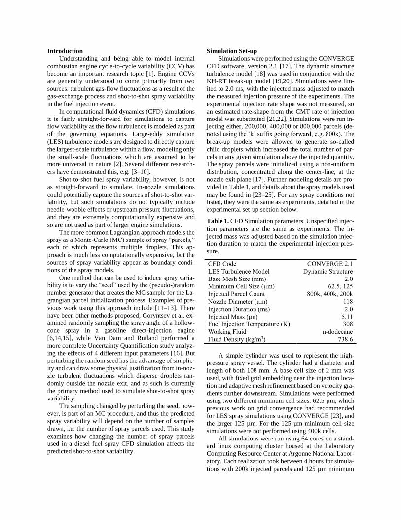
chamber was measured with a PIN diode. A schematic

of the set-up is given in Figure 1.

Figure 1. Schematic of the x-ray radiography set-up. X-

rays travel from right to left in the image.

The x-ray beam was focused to a relatively small

spot-size of approximately 5x6 µm. To build the 2D data

field, measurements were made for different spray

events at many different raster-scan positions. For the

current study, approximately 750 points were used as

part of the raster grid at locations across the spray width

and as far as 9 mm downstream of the nozzle exit. A plot

of the raster positions is shown in Figure 2. Visualization

was performed by interpolating the measurements from

the raster locations to a regular grid with Δ𝑋 ≈ 45 µm

and Δ𝑌 ≈ 4.6 µm. No extrapolation was used for points

on the visualization grid outside the convex hull of the

raster points, these points were simply assigned PMD

values of zero. The same visualization procedure was

used for simulations to maintain consistency.

Figure 2. X-ray measurement grid. The nozzle-hole exit

is located at (0,0). The injector axis is along the Y=0 plot

axis and the spray travels in the positive X direction.

At each raster point, the full time-history of 32 sep-

arate injection events was recorded to allow for calcula-

tion of ensemble mean and standard deviation (SD) sta-

tistics. For comparison with simulations time-averaging

was also used once the near-nozzle region investigated

by the x-ray measurements reached a quasi-steady state.

Using the x-ray beam intensity time-histories the

PMD was calculated using the Beer-Lambert law:

𝐼(𝑥, 𝑦, 𝑡)

𝐼0(𝑥, 𝑦)= 𝑒−𝜇𝑀(𝑥,𝑦,𝑡) (1)

where 𝐼0(𝑥, 𝑦) is the baseline beam intensity, i.e. without

any spray, 𝐼(𝑥, 𝑦, 𝑡) is the beam intensity during the

spray, 𝜇 the mass absorption coefficient and 𝑀(𝑥, 𝑦, 𝑡)

the PMD. The mass absorption coefficient is determined

from a calibration procedure with fuel from the experi-

ments placed in a cuvette of known size.

The transverse integrated mass (TIM) and trans-

verse integrated fluctuations (TIF) are two further quan-

tities derived from the PMD measurements. They are re-

lated to the local spray velocity and also present a way to

compare sprays that is independent of local spray width.

They are calculated from the PMD by integrating in the

transverse direction across the spray (i.e. the Y-direction

in the current coordinate system, which is shown in Fig-

ure 2):

𝑇𝐼𝑀(𝑥, 𝑡) = ∫ 𝑀(𝑥, 𝑦, 𝑡)

∞

−∞

d𝑦 (2)

𝑇𝐼𝐹(𝑥, 𝑡) = ∫ 𝑀′(𝑥, 𝑦, 𝑡)

∞

−∞

d𝑦 (3)

In this study a single-hole hydro-ground research

diesel injector was used. The injector had a conical noz-

zle geometry with K=1.5, and a nominal nozzle hole size

of 110 µm though later x-ray tomography measurements

showed an actual diameter of 118 µm. All simulations

presented in this work used 118 µm as the nozzle-hole

diameter.

Fuel was supplied through an automotive diesel

common-rail injection system. The injection pressure

was set to 500 bar. The ambient gas was at room temper-

ature, with a pressure of 20 bar absolute. The working

fluid used for the injections was a diesel calibration fluid

(Viscor 1487) doped with 4% by weight cerium additive

to increase x-ray absorptivity. The resulting fuel had a

higher density than the standard simulation diesel surro-

gate n-dodecane. A density correction was applied to the

simulation results to account for this.

Other experimental details are listed in Table 2. Fur-

ther details of the experimental set-up and measurement

techniques may be found in [26].

Table 2. Experimental measurement details. The esti-

mated injector nozzle diameter was found as described

in the text.

Nozzle Diameter (µm) 118

Injection Pressure (bar) 500

Ambient Pressure (bar) 20

Ambient Temperature (K) 298

Working Fluid Viscor 1487+

Rhodia DPX9

Fluid Density (kg/m3) 866.4

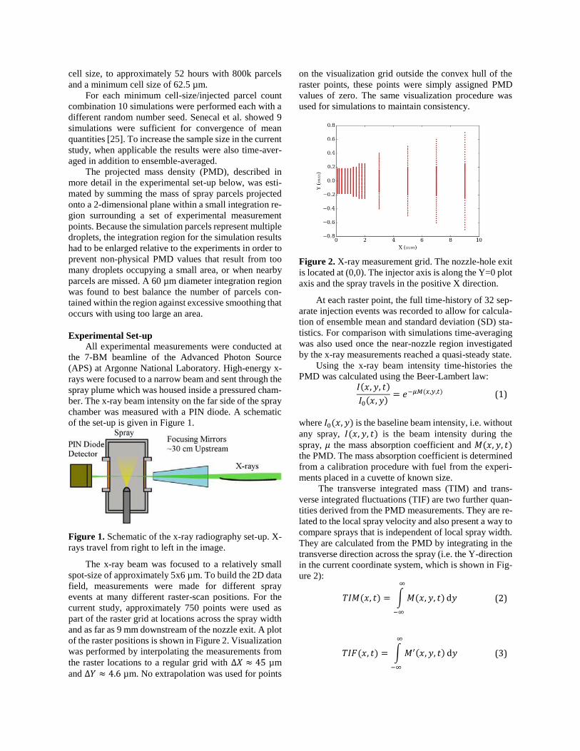
Liquid Penetration

Experimental liquid penetration data is derived from

the PMD measurements. Because the PMD measure-

ments were only taken in the near-nozzle region, up to 9

mm downstream of the nozzle exit, the measured liquid

penetration is also limited to this near-nozzle region. Fig-

ure 3 plots the mean liquid penetration from experiments

as well as simulations at the two different minimum cell

sizes and 3 different injected parcel counts in the near-

nozzle region. Changing the injected parcel count does

not affect the liquid penetration in this portion of the

spray. There are some differences based on the minimum

cell size. The simulations match experimental data very

close to the nozzle exit, but begin to over penetrate rela-

tive to the experimental results after approximately 0.03

ms after start-of-injection (SOI), when the sprays have

reached approximately 2 mm downstream of the nozzle

exit.

Figure 3. Near-nozzle liquid penetration for experiments

and simulations with different injected parcel counts and

minimum cell sizes.

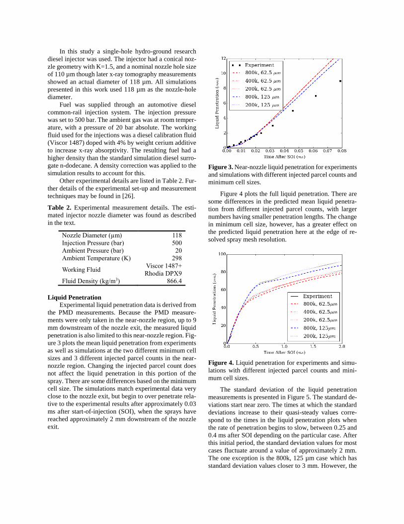
Figure 4 plots the full liquid penetration. There are

some differences in the predicted mean liquid penetra-

tion from different injected parcel counts, with larger

numbers having smaller penetration lengths. The change

in minimum cell size, however, has a greater effect on

the predicted liquid penetration here at the edge of re-

solved spray mesh resolution.

Figure 4. Liquid penetration for experiments and simu-

lations with different injected parcel counts and mini-

mum cell sizes.

The standard deviation of the liquid penetration

measurements is presented in Figure 5. The standard de-

viations start near zero. The times at which the standard

deviations increase to their quasi-steady values corre-

spond to the times in the liquid penetration plots when

the rate of penetration begins to slow, between 0.25 and

0.4 ms after SOI depending on the particular case. After

this initial period, the standard deviation values for most

cases fluctuate around a value of approximately 2 mm.

The one exception is the 800k, 125 µm case which has

standard deviation values closer to 3 mm. However, the

reported liquid penetration standard deviations fluctuate

as much as 1.5 mm in time. It should also be kept in mind

that since liquid penetration is only ensemble-averaged,

there are only 10 samples in the standard deviation fig-

ures, and thus the 95% confidence intervals (not shown)

are much larger than any differences shown in the figure.

It is therefore difficult to make any definitive compari-

sons between the simulation results.

Figure 5. Standard deviation of liquid penetration for

simulations with different injected parcel counts and

minimum cell sizes.

Projected Mass Density

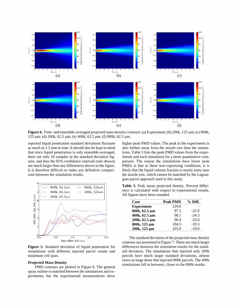
PMD contours are plotted in Figure 6. The general

spray outline is matched between the simulations and ex-

periments, but the experimental measurements show

higher peak PMD values. The peak in the experiments is

also further away from the nozzle exit than the simula-

tions. Table 3 lists the peak PMD values from the exper-

iments and each simulation for a more quantitative com-

parison. The reason the simulations have lower peak

PMDs is that at these non-vaporizing conditions, it is

likely that the liquid volume fraction is nearly unity near

the nozzle exit, which cannot be matched by the Lagran-

gian parcel approach used in this study.

Table 3. Peak mean projected density. Percent differ-

ence is calculated with respect to experimental results.

All figures have been rounded.

Case Peak PMD % Diff.

Experiment 129.6 -

800k, 62.5 µm 97.1 -25.0

400k, 62.5 µm 98.1 -24.3

200k, 62.5 µm 96.4 -25.6

800k, 125 µm 104.5 -19.3

200k, 125 µm 105.0 -19.0

The standard deviation of the projected mass density

contours are presented in Figure 7. There are much larger

differences between the simulation results for the stand-

ard deviation. The simulations that injected only 200k

parcels have much larger standard deviations, almost

twice as large those that injected 800k parcels. The 400k

simulations fall in between, closer to the 800k results.

(a) (b) (c)

(d) (e) (f)

Figure 6. Time- and ensemble-averaged projected mass density contours: (a) Experiment; (b) 200k, 125 µm; (c) 800k,

125 µm; (d) 200k, 62.5 µm; (e) 400k, 62.5 µm; (f) 800k, 62.5 µm.

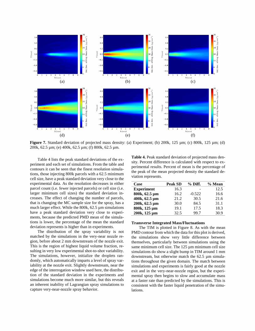
Table 4 lists the peak standard deviations of the ex-

periment and each set of simulations. From the table and

contours it can be seen that the finest resolution simula-

tions, those injecting 800k parcels with a 62.5 minimum

cell size, have a peak standard deviation very close to the

experimental data. As the resolution decreases in either

parcel count (i.e. fewer injected parcels) or cell size (i.e.

larger minimum cell sizes) the standard deviation in-

creases. The effect of changing the number of parcels,

that is changing the MC sample size for the spray, has a

much larger effect. While the 800k, 62.5 µm simulations

have a peak standard deviation very close to experi-

ments, because the predicted PMD mean of the simula-

tions is lower, the percentage of the mean the standard

deviation represents is higher than in experiments.

The distribution of the spray variability is not

matched by the simulations in the very-near nozzle re-

gion, before about 2 mm downstream of the nozzle exit.

This is the region of highest liquid volume fraction, re-

sulting in very low experimental shot-to-shot variability.

The simulations, however, initialize the droplets ran-

domly, which automatically imparts a level of spray var-

iability at the nozzle exit. Slightly downstream, near the

edge of the interrogation window used here, the distribu-

tion of the standard deviation in the experiments and

simulations become much more similar, but this reveals

an inherent inability of Lagrangian spray simulations to

capture very-near-nozzle spray behavior.

Table 4. Peak standard deviation of projected mass den-

sity. Percent difference is calculated with respect to ex-

perimental results. Percent of mean is the percentage of

the peak of the mean projected density the standard de-

viation represents.

Case Peak SD % Diff. % Mean

Experiment 16.3 - 12.5

800k, 62.5 µm 16.2 -0.522 16.6

400k, 62.5 µm 21.2 30.5 21.6

200k, 62.5 µm 30.0 84.5 31.1

800k, 125 µm 19.1 17.5 18.3

200k, 125 µm 32.5 99.7 30.9

Transverse Integrated Mass/Fluctuations

The TIM is plotted in Figure 8. As with the mean

PMD contour from which the data for this plot is derived,

the simulations show very little difference between

themselves, particularly between simulations using the

same minimum cell size. The 125 µm minimum cell size

simulations do show a slight bump in TIM around 1 mm

downstream, but otherwise match the 62.5 µm simula-

tions throughout the given domain. The match between

simulations and experiments is fairly good at the nozzle

exit and in the very-near-nozzle region, but the experi-

mental spray then begins to slow and accumulate mass

at a faster rate than predicted by the simulations. This is

consistent with the faster liquid penetration of the simu-

lations.

(a) (b) (c)

(d) (e) (f)

Figure 7. Standard deviation of projected mass density: (a) Experiment; (b) 200k, 125 µm; (c) 800k, 125 µm; (d)

200k, 62.5 µm; (e) 400k, 62.5 µm; (f) 800k, 62.5 µm.

Figure 8. Transverse integrated mass for experiments

and simulations with different injected parcel counts and

minimum cell sizes.

The TIF is plotted in Figure 9, and shows much

greater differences between the simulations. As with the

PMD contours, the primary difference among the simu-

lations is due to changing the number of parcels injected,

rather than differences in the minimum cell size used.

The simulations with 800k parcels lie closest to the ex-

perimental data, though still slightly higher. The simula-

tions also do not match the experimentally measured re-

gion of low TIF near the nozzle exit, again because the

Lagrangian parcel approach imposes a certain level of

variability in the spray due to the initialization proce-

dure.

Figure 9. Transverse integrated fluctuations for experi-

ments and simulations with different injected parcel

counts and minimum cell sizes.

Conclusions

Multiple realizations of large-eddy spray simula-

tions were run using different numbers of injected La-

grangian parcels and different minimum cell sizes. The

predicted mean quantities were nearly independent of the

number of parcels used in this study, while some depend-

ence on the minimum cell size was seen. This is expected

because the minimum cell sizes chosen here are at and

slightly above the converged cell sizes found in previous

work.

The Lagrangian spray modeling approach is based

on an MC sampling approach to the spray, and as such

the number of injected parcels significantly affects the

variability of the simulations. The standard deviation of

projected mass density doubled as the number of parcels

injected changed from 800k to 200k. 800k parcels is

many more than is typically used in spray calculations,

particularly those that are part of full engine simulations,

but the results here show that changing the number of

parcels will have a significant effect on the shot-to-shot

spray variability seen when perturbing the random seed.

Simply perturbing the random seed is an easy and

quick way to induce shot-to-shot spray variability in La-

grangian CFD simulations, but the parcel count sample

size effect must be understood and taken into considera-

tion in future studies of shot-to-shot or cycle-to-cycle

variability that rely on random seed perturbations.

Acknowledgment

The submitted manuscript has been created by

UChicago Argonne, LLC, Operator of Argonne National

Laboratory (Argonne). Argonne, a U.S. Department of

Energy Office of Science laboratory, is operated under

contract No. DE-AC02-06CH11357. The U.S. Govern-

ment retains for itself, and others acting on its behalf, a

paid-up nonexclusive, irrevocable worldwide license in

said article to reproduce, prepare derivative works, dis-

tribute copies to the public, and perform publicly and dis-

play publicly, by or on behalf of the Government. This

research was funded by U.S. DOE Office of Vehicle

Technologies, Office of Energy Efficiency and Renewa-

ble Energy under Contract No. DE-AC02-O6CH11357.

Experimental measurements were performed at the

7-BM beamline of the Advanced Photon Source at Ar-

gonne National Laboratory. Use of the APS is supported

by the U.S. Department of Energy (DOE) under Contract

No. DE-AC02-06CH11357.

The authors wish to thank Gurpreet Singh and Leo

Breton, program managers at DOE, for their support.

The computing resources were provided by the La-

boratory Computing Resource Center at Argonne Na-

tional Laboratory.

The authors would like to acknowledge Convergent

Sciences Inc. for providing CONVERGETM licenses

which were used for this work.

The authors would like to thank Ron Grover for in-

itial discussions on this topic. They also thank Lyle

Pickett for use of the fuel injection nozzle analyzed in

this work.

Nomenclature

I X-ray beam intensity

𝜇 Mass absorption coefficient

M Projected mass density

Abbreviations

APS Advanced Photon Source

CCV Cycle-to-cycle variation

CFD Computational fluid dynamics

LES Large-eddy simulation

MC Monte-Carlo

PMD Projected mass density

SD Standard deviation

SOI Start-of-injection

TIF Transverse integrated fluctuations

TIM Transverse integrated mass

Suffixes

k Thousand

References

1. W. Eckerle, and C. Rutland, “A Workshop to

Identify Research Needs and Impacts in Predictive

Simulation for Internal Combustion Engines

(PreSICE).”

2. S.B. Pope, Turbulent Flow, Cambridge University

Press, 2000.

3. V. Granet, O. Vermorel, C. Lacour, B. Enaux, V.

Dugué, and T. Poinsot, Combustion and Flame

159:1562–1575 (2012).

4. A. Banaeizadeh, A. Afshari, H. Schock, and F.

Jaberi, International Journal of Heat and Mass

Transfer 60:781–796 (2013).

5. S. Fontanesi, S. Paltrinieri, A. Tiberi, and A.

D’Adamo, SAE Technical Paper 2013-01-1080

(2013).

6. D. Goryntsev, A. Sadiki, and J. Janicka, SAE

Technical Paper 2012-01-0399 (2012).

7. T. Kuo, X. Yang, V. Gopalakrishnan, and Z. Chen,

Oil & Gas Science and Technology – Revue d’IFP

Energies nouvelles 69:61–81 (2013).

8. J. Koch, M. Schmitt, Y.M. Wright, K. Steurs, and

K. Boulouchos, SAE International Journal of

Engines 7 (2014).

9. D.C. Haworth, A. Anand, T.-W. Kuo, D.L. Reuss,

C.J. Rutland, V. Sick, P. Schiffmann, Y.

Shekhawat, N. Van Dam, and X. Yang, 9th U. S.

National Combustion Meeting, 2015.

10. N. Van Dam, and C. Rutland, Proceedings of the

2015 ASME Internal Combustion Engine Division

Fall Technical Conference, November 2015.

11. C. Habchi, and G. Bruneaux, 12th Triennial

International Conference on Liquid Atomization

and Spray Systems, September 2012.

12. Y. Pei, S. Som, E. Pomraning, P.K. Senecal, S.A.

Skeen, J. Manin, and L.M. Pickett, Combustion

and Flame 162:4442–4455 (2015).

13. M.M. Ameen, Y. Pei, and S. Som, SAE Technical

Paper 2016-01-0585 (2016).

14. D. Goryntsev, A. Sadiki, and J. Janicka, SAE

Technical Paper 2011-01-1884 (2011).

15. D. Goryntsev, K. Nishad, A. Sadiki, and J. Janicka,

Oil & Gas Science and Technology – Revue d’IFP

Energies nouvelles 69:129–140 (2013).

16. N. Van Dam, and C. Rutland, International

Journal of Engine Research 17:291–315 (2016).

17. K. Richards, P. Senecal, and E. Pomraning,

“Converge (Version 2.1.0) Manual.”

18. E. Pomraning, and C.J. Rutland, AIAA Journal

40:689–701 (2002).

19. R.D. Reitz, Atomisation and Spray Technology

3:309–337 (1987).

20. M.A. Patterson, and R.D. Reitz, SAE Technical

Paper 980131 (1998).

21. R. Payri, F.J. Salvador, J. Gimeno, and G. Bracho,

Experimental Techniques 32:46–49 (2008).

22. L.M. Pickett, J. Manin, R. Payri, M. Bardi, and J.

Gimeno, SAE Technical Paper 2013-24-0001

(2013).

23. P.K. Senecal, E. Pomraning, K.J. Richards, and S.

Som, SAE Technical Paper 2013-01-1083 (2013).

24. Q. Xue, S. Som, P.K. Senecal, and E. Pomraning,

Atomization and Sprays 23:925–955 (2013).

25. P.K. Senecal, E. Pomraning, Q. Xue, S. Som, S.

Banerjee, B. Hu, K. Liu, and J.M. Deur, Journal of

Engineering for Gas Turbines and Power

136:111504 (2014).

26. A.B. Swantek, D.J. Duke, C.F. Powell, and A.L.

Kastengren, JSAE Technical Paper 20159308

(2015).