THE EFFECTS OF INTERNATIONAL TRADE ON ECONOMIC GROWTH …
108
THE EFFECTS OF INTERNATIONAL TRADE ON ECONOMIC GROWTH IN SOUTH AFRICA (2000Q1 TO 2017Q1) AND ECONOMETRIC VIEW NDIVHUHO EUNICE RATOMBO Dissertation submitted for the requirements for the degree of MASTER OF COMMERCE IN ECONOMICS in FACULTY OF MANAGEMENT & LAW (School of Economics and Management) at the UNIVERSITY OF LIMPOPO SUPERVISOR: Prof IP MONGALE 2019
Transcript of THE EFFECTS OF INTERNATIONAL TRADE ON ECONOMIC GROWTH …

THE EFFECTS OF INTERNATIONAL TRADE ON ECONOMIC GROWTH IN
SOUTH AFRICA (2000Q1 TO 2017Q1) AND ECONOMETRIC VIEW
NDIVHUHO EUNICE RATOMBO
Dissertation submitted for the requirements for the degree of
MASTER OF COMMERCE IN ECONOMICS
in
FACULTY OF MANAGEMENT & LAW
(School of Economics and Management)
at the
UNIVERSITY OF LIMPOPO
SUPERVISOR: Prof IP MONGALE
2019
ii
DECLARATION
I declare that THE EFFECTS OF INTERNATIONAL TRADE ON ECONOMIC GROWTH
IN SOUTH AFRICA (2000Q1 TO 2017Q1) AND ECONOMETRIC VIEW is my
own work and that all the sources that I have used or quoted have been indicated and acknowledged
by means of complete references and that this work has not been submitted before for any other
degree at any other institution.
Ndivhuho Eunice Ratombo 25 March 2019
Full names Date

iii
ACKNOWLEDGEMENTS
Undertaking a research project of this type is necessarily demanding, nevertheless there are so
many important people who supported me in different ways during the development of this
dissertation that I would like to thank. Indeed, without their support, guidance, advice and
encouragement the completion of my research study would not have been possible.
First I would like to thank the Almighty God for giving me the ability to complete my dissertation.
Again I would like to extend a sincere thank you to my supervisor, Prof Itumeleng Mongale; it
was such an honour working with him, his guidance, support and encouragement are greatly
appreciated. Prof Ncanywa and Prof Mah thank you for the support. Apostle/Senior Pastor M.M
and Pastor V.J Ratombo, Pastor Maurice and Nokuthula, and the Ratombo family for being my
source of inspiration throughout the duration of the study, especially my mother Mrs NT Ratombo
whose prayers propelled me to this point. Mr K Vhengani and my son Akonaho Munangiwa, Mr
T and R.J Khumisi, The BBC family, My fellow students Manyaka K, Baloyi L, Mulaudzi MP
and all masters of economics students at the University of Limpopo. Thank you all so much for
your flexibility, understanding, openness, willingness and support throughout the entire process.

iv
ABSTRACT
International trade has been identified by many economists to be an engine for growth and
development. There has been an increase in the number of bilateral and multilateral trade
agreements across the globe. Trade has gained significant attention among developed and
developing countries and it hugely attributed to the impact of technology and globalisation. The
study employs autoregressive distributed lag (ARDL) bounds testing approach to analyse The
effects of international trade on economic growth in South Africa from (2000Q1 to 2017Q1) and
economic review. The quarterly time series data from 2000Q1 to 2017Q1 is sourced from the
South African Reserve Bank (SARB) and Quantec Easy Data. This study is envisaged to provide
a better understanding on the relationship between South African economic growth and
international trade. The findings brought light on how growth can be improved in South Africa.
The unit root tests indicate a mixture of I(0) and I(1) variables which implied the employment of
the ARDL approach. The cointegration model emphasizes the long-run equilibrium relationship
between the dependant and independent variables. The findings reveal that exchange rate and
import are positively related with GDP while one export is negatively related to it. The conclusion
from this work is that there is correlation between GDP and its regressors. Since the results show
that South African export have negative impact on growth, it is recommended that South African
government must promote trading of goods and services internally and not focus much on exporting its
primary goods and services abroad because it weakens the economy. It is recommended that South
Africa must produce or export according to the need of the industry, so that the country benefit in
return. Lastly, it is recommended that South Africa must support local industries and firms to create
more employment opportunities and start programmes that will make youth to be active in
businesses and reduce over reliance to the government.
KEY CONCEPTS: Economic growth, International trade, ARDL approach, South Africa, GDP

v
TABLE OF CONTENTS
DECLARATION ............................................................................................................................ ii
ACKNOWLEDGEMENTS ........................................................................................................... iii
ABSTRACT ................................................................................................................................... iv
ACRONYMS ............................................................................................................................... viii
LIST OF FIGURES ....................................................................................................................... ix
LIST OF TABLES .......................................................................................................................... x
CHAPTER 1 ................................................................................................................................... 1
ORIENTATION TO THE STUDY ................................................................................................ 1
1.1 INTRODUCTION AND BACKGROUND ........................................................................ 1
1.2 STATEMENT OF THE PROBLEM .................................................................................. 4
1.3 RESEARCH QUESTIONS ................................................................................................. 5
1.4 RESEARCH AIM AND OBJECTIVES ............................................................................. 5
1.4.1 Aim ...................................................................................................................................... 5
1.4.2 Objectives ............................................................................................................................ 5
1.5 DEFINITION OF CONCEPTS........................................................................................... 6
1.6 ETHICAL CONSIDERATIONS ........................................................................................ 7
1.7 SIGNIFICANCE OF THE STUDY .................................................................................... 7
LITERATURE REVIEW ............................................................................................................... 9
2.1 Introduction ......................................................................................................................... 9
2.2 Theoretical Framework ....................................................................................................... 9
2.2.1 Classical period: international trade and growth ................................................................ 9
2.2.2 Post classical period: international trade and growth ......................................................... 9
2.2.2.1 Neoclassical International theory ...................................................................................... 10

vi
2.2.2.2 The Neoclassical paradigm ............................................................................................... 10
2.2.3 Post-classical growth before Solow ..................................................................................... 11
2.3 Empirical literature............................................................................................................ 11
2.3.1 Exchange rate theory ............................................................................................................ 16
2.3.2 Some theories on how international trade benefits can be shared among countries are
discussed below:- .......................................................................................................................... 18
2.4 Summary ........................................................................................................................... 22
CHAPTER 3 ................................................................................................................................. 23
RESEARCH METHODOLOGY.................................................................................................. 23
3.1 Introduction ....................................................................................................................... 23
3.2 Data ................................................................................................................................... 23
3.3 Model specification ........................................................................................................... 23
3.4 Estimation techniques ....................................................................................................... 24
3.4.1 Stationarity/Unit root test .................................................................................................. 25
3.4.1.1 Visual inspection ............................................................................................................... 25
3.4.1.2 Formal unit root tests ........................................................................................................ 25
3.4.1.2.1 Augmented Dickey Fuller (ADF) test ........................................................................ 25
3.4.1.2.2 Phillips-Perron (PP) test ............................................................................................. 26
3.4.1.2.3 Dickey Fuller Generalized Least Squares (DF-GLS) test .......................................... 27
3.4.2 ARDL Bounds Testing Procedure .................................................................................... 27
3.4.3 Diagnostic testing .............................................................................................................. 29
3.4.3.1 Serial correlation ............................................................................................................... 29
3.4.3.2 Heteroskedasticity ............................................................................................................. 29
3.4.3.3 Normality test .................................................................................................................... 29
3.4.3.4 Autocorrelation ................................................................................................................. 30
3.4.4 Stability testing ................................................................................................................. 31

vii
3.4.5 Error Correction Model (ECM) ........................................................................................ 32
3.5 Summary ........................................................................................................................... 32
CHAPTER 4 ................................................................................................................................. 33
DISCUSSION / PRESENTATION / INTERPRETATION OF FINDINGS ............................... 33
4.1 Introduction ....................................................................................................................... 33
4.2 Empirical tests results ....................................................................................................... 33
4.2.1 Stationarity/Unit root tests results ..................................................................................... 33
4.2.1.1 Visual inspection ............................................................................................................... 33
4.2.1.2 Formal unit root tests results ............................................................................................. 34
4.2.2 Bounds test results ............................................................................................................ 37
4.2.3 ARDL long-run coefficients model .................................................................................. 38
4.2.4 Diagnostic tests results ...................................................................................................... 42
4.3 Summary ........................................................................................................................... 44
CHAPTER 5 ................................................................................................................................. 45
SUMMARY, RECOMMENDATIONS, CONCLUSION ........................................................... 45
5.1 Introduction ....................................................................................................................... 45
5.2 Summary and Interpretation of Findings .......................................................................... 45
5.3 Conclusions ....................................................................................................................... 45
5.4 Limitations of the study .................................................................................................... 46
5.5 Policy recommendations ................................................................................................... 46
APPENDIX A: ADF TEST UNIT ROOT TESTS .................................................................... 55
APPENDIX B: PHILLIPS-PERRON UNIT ROOT TESTS ................................................... 70
APPENDIX C: DF-GLS UNIT ROOT TESTS ............................................................................ 77
APPENDIX D: ARDL COINTEGRATING AND LONG RUN FORM ..................................... 94
APPENDIX E: RAMSEY RESET ............................................................................................... 97
viii
ACRONYMS
ASGISA- Accelerated and Shared Growth Initiative for South Africa
GDP- Gross Domestic Product
OLS- Ordinary Least Squares
ARDL- Autoregressive Distributed Lag
ADF- Augmented Dickey Fuller
DF- GLS-Dickey Fuller Generalized Least Squares
PP- Phillip-Perron
IT- International Trade
EG- Economic Growth
IS- Import Substitution
EP- Export Promotion
IR- Industrial Revolution
SARB- South African Reserve Bank
OECD- Organisation for Economic Co-operation and Development
R&D- Research and Development
HOS- Heckscher-Ohlin-Samuelson
FDI- Foreign Direct Investment

ix
LIST OF FIGURES
Figure 4.1 GDP at level 34
Figure 4. 2 GDP at first difference 34
Figure 4.3 Normality test results 42

x
LIST OF TABLES
Table 4.1: Augmented Dickey Fuller test at level ......................................................... 34
Table 4.2: Augmented Dickey Fuller test at 1st difference ............................................ 35
Table 4.3: Phillips Perron test at level ........................................................................... 35
Table 4.4: Phillips Perron test at 1st difference .............................................................. 36
Table 4.5: Dickey Fuller Generalized Least Squares test at level ................................. 36
Table 4.6: Dickey Fuller Generalized Least Squares test at 1st difference .................... 37
Table 4.7: Bounds test .................................................................................................... 38
Table 4.8: Lower and Upper bound test by Persaran et al. ............................................ 38
Table 4.9: ARDL long-run coefficients model .............................................................. 38
Table 4.10: Error Correction Model .............................................................................. 41
Table 4.11: Stability Diagnostic check .......................................................................... 42
Table 4.12: Ramsey Reset .............................................................................................. 44

1
CHAPTER 1
ORIENTATION TO THE STUDY
1.1 INTRODUCTION AND BACKGROUND
International trade has been identified by many economists to be an engine for growth and
development. International trade has experienced mixed results on growth and development.
Presently there is no country around the world that does not trade; hence there has been an
increase in the number of bilateral and multilateral trade agreements across the globe.
International trade among nations has gained significant attention among both developed and
developing countries; it is hugely attributed to the impact of technology and globalisation
(Nageri, Olodo, Bukulo and Babatunde, 2013).
The issue of international trade and economic growth have gained substantial importance with
the introduction of trade liberalization policies in the developing nations across the world.
International trade and its impact on economic growth crucially depend on globalization.
Impact of international trade on economic growth divided economists of the developed and
developing countries into two separate groups. One group of economists believed that
international trade has brought unfavourable changes in economic and financial scenarios of
the developing countries. Meaning that gains from trade benefited developed nations of the
world (Vijayasri 2013).
The other group of economists speak in favour of globalization and international trade with a
brighter view of the international trade and its impact on economic growth of the developing
nations. According to this group of economists, developing countries which have followed
trade liberalization policies have experienced all the favourable effects of globalization and
international trade. There is no denying that international trade is beneficial for the countries
involved in trade, if practiced properly (Vijayasri 2013).
The importance of international trade stems from the fact that no country can produce all goods
and services which people require for their consumption largely owing to resources differences
and constraints. As a result, this trade relationship suggests that economies need to export
goods and services in order to generate revenue to finance imported goods and services which
cannot be produced domestically (Adeleye, Adewuyi and Adeteye, 2015).

2
The effects of international trade on a nation are neither direct nor indirect. The effects of
international trade are both positive and negative, it is a two-way process where the country
neither benefit nor lose. The direct effects relate to bilateral trade between countries, whereas
the indirect effect involves competing with other countries in a third market. Below, the
researcher illustrated some of the effects of international trade on participating countries: -
Firstly, international trade affects employment opportunities in both importing and exporting
countries. Developing countries have been experiencing loss of “good” manufacturing jobs as
a result of import competition; conversely there is an increase in “bad” jobs which hamper
exports in developing countries. Job losses results in both political and economic instabilities,
which retard economic growth (Jenkins and Sen, 2006).
Secondly, international trade affects commodity prices, but mostly in importing countries.
Import competition drives prices down. The impact of the import flow from low-income
countries on developed countries’ prices is more pronounced in sectors with an elastic demand.
This is due to the fact that it is easier for foreign firms to penetrate a market with elastic demand.
The response of prices to a percentage increase in import competition is higher in sectors with
inelastic demand. As highlighted by Auer (2008:3), the Import effect on sectors with different
elasticity of demand is larger in the short run than in the long run. According to Unite Nation
report cited in Auer and Fischer (2008) it has been revealed that the combined effect of higher
prices of commodity exports and lower prices of exports of labour-intensive manufacturers is
more pronounced in countries exporting primary commodities and this has been noted in Latin
American countries (e.g. Brazil and Mexico), as well as in South Africa. Lastly, international
trade affects industrial productivity. Compositional theory suggests lower trade cost induces
firms to change their product mix so that it can fit in the existing menu of products. This is
mostly a result of importing from low-cost countries that reduces a firm’s production costs.
Firms will tend to move to producing high-technological commodities if the fall in trade cost
occurs with low-wage countries. It is a challenge to developing countries because they cannot
read the signs of growth on the international market, they act only after the developed countries
has done so.
The participation in international trade and an improvement in export performance as believed
by many economists contribute largely to developing countries’ economic growth since the
1960s and 1970s (Ahmend, Cheng and Messinis, 2008). International trade creates economic
incentives that boost productivity through two dynamics: - in the short-run trade reduces

3
resource use misallocation while in the long-run it facilitates transfer of technological
development. Trade can also force government to commit to reform programs under the
pressure of international competition while enhancing economic growth. It is also in the hands
of nations or country to see how they pave the way for their economy to grow (Sachs and
Warner, 1995; Rajan and Zingales 2003). International trade is one of the leading and trending
discussions taken not only in South Africa but worldwide on daily basis. International trade is
important because one country can assist the other country to meet its needs, which can help
develop the level of economic growth of the assisted country (Mogoe, 2013).
There have been increasing arguments and discussions in favour of export-led strategy
development stating that an expansion of international trade will enhance productivity through
increased economies of scale in the export sector, productivity will be positively affected
through an increase in better allocation of resources which will be driven by specialization and
increase in efficiency. In the long-run, this will generate dynamic comparative advantage
through reduction in costs for the exporting country. Another advantage in the export-led
strategy is through the process of interaction with the international markets, there will be
diffusion or exchange of knowledge through learning by-by-doing and a greater efficiency in
management through efficient management techniques which will have a net positive effect on
the other parts of the economy (Ahmend et al., 2008).
International trade might constitute an effective channel for international transmission of know-
how and dissemination of technological progress. In emerging economies, openness to
international trade could be a means of overcoming the narrowness of the domestic market and
provide an outlet for surplus products in relation to domestic requirements. Extension of the
market size due to export orientation can bring economies of scale in the required production
processes. Exposure to new products such as import of high technological inputs, new
advanced methods and production processes could stimulate technological upgrades and
greater development (Deumal and Ozyurt, 2011).
Trade in Africa as a share of Gross Domestic Product (GDP) increased from 38% to 43%
between 1988 to 1989 and 1999 to 2000, respectively. African continent has been resisting
open trade regimes instead of focusing on growth enhancing policies including promotion of
exports of dynamic products. The region’s export share in the global market decline to about
3.1% which was almost half of the original growth rate, but with time, as most African
countries began to open up their markets to the rest of the world; the share of exports in GDP

4
has reversed its descent (Ahmend et al., 2008). The adoption of the Accelerated and Shared
Growth Initiative for South Africa (ASGISA) in February 2006 signalled the Government
intention to pursue a developmental strategy that will promote and accelerate economic growth
along a path that generates sustainable and decent jobs. Although the role international trade
can play in this endeavour should not be exaggerated because other factors such as commodity
prices, investment rates, global and national demand can be more decisive in shaping the
economic growth path. With time, between 1994 and 2002, growth in South Africa averaged
around 3% annually - this accelerated to an average of over 5% for the five years ending in
2008. This led to a virtuous combination of positive domestic sentiment and a favourable
international environment created the basis for eight years of uninterrupted growth (Davies,
2010).
1.2 STATEMENT OF THE PROBLEM
Since the initiation of economic reforms and the adoption of the door policy, international trade
and South African economy have experienced dramatic growth in 1994. According to Du
Plessis (2014), in the year 1994 democratic transition created turnaround in the South African
economic performance. Due to little openness to international trade South Africa is failing to
improve its economic growth which lead to inadequate infrastructure, high levels of
unemployment, limited growth path and unsustainable growth. These trade barriers promote
trade deficit in many African countries, neglect long-term growth and fail to sustain future
growth.
The growth performance of the South African economy has been neglected and this has lead
the country to face rising interest rates which lead to strong credit growth, widen current
account deficit and high inflation which restricted consumer spending on their own produce.
South Africa growth is highly resource intensive, specialising in exporting primary agricultural
products which are unsustainable and hence, address the needs of the most developing
countries without support to promote rapid economic growth. The country has been under
pressure with the declining or non-stability in the value of the currency (Rand), which caused
export performance to be pressurised.
For South Africa, endowments of natural resources or basic industries are no longer necessary
or sufficient for participation in this new global environment. International trade is a substitute
for self-sufficiency at all stages in product value chains and if these raw materials are not
managed properly there can be hindrance rather than solution to economic growth (Stern and

5
Flatters, 2007). South Africa must use international trade and capital flows as their main keys
to openness and strength to rapid growth in global market to close the gap that was lagged
behind. Another study by Mogoe (2013), indicate that export is important on international trade
since it can create growth and expansion at the same time
The previous studies did not mention whether the effects of international trade had led to
increase or decrease on economic growth in South Africa. Most of the previous studies on
international trade and economic growth in South Africa have used ADF unlike this study
where ARDL is used. Most studies focus on two or three variables unlike this one which
focuses on four variables to bring out change and come up with measures that will strengthen
the country’s growth. In South Africa economic growth and international trade are not
happening at the same time, and if the two are moving in different or parallel directions, it is
difficult to enjoy the benefits of international trade. Thus, the current study or methodology
sought to investigate the effects of international trade on economic growth in South Africa
during the period 2000Q1 to 2017Q1 using quarterly data. The study further seeks to determine
whether international trade presents export and imports opportunities for economic growth in
South Africa.
1.3 RESEARCH QUESTIONS
Does international trade promote economic growth?
Does international trade promote exchange rate in South Africa?
Does international trade promote export?
1.4 RESEARCH AIM AND OBJECTIVES
1.4.1 Aim
The aim of this study is to analyse the effect of international trade on economic growth in
South Africa from 2000Q1 to 2017Q1.
1.4.2 Objectives
The following objectives will be used to reach the main aim:
To examine the relationship between international trade and economic growth.
To examine the relationship between international trade and exchange rate.
To examine the relationship between international trade and export.
The stated objectives will be attained by the use of ARDL framework.

6
1.5 DEFINITION OF CONCEPTS
1.5.1 Economic growth
According to Lopez (2005) economic growth means the steady process by which the productive
capacity of the economy is increased over time to bring about rising levels of national output
and income. In contrast, Mankiw (2011) defined economic growth as the increase in the
amount of goods and services in an economy over a period of time; it is also caused by rising
number of labour force in the market.
1.5.2 International trade
International trade is known as the exchange of goods and services between nations of the
world. At least two countries should be involved, that is the aggregate of activities relating to
trading between merchants across borders. Traders engage in economic activities for the
purpose of the profit maximization engendered from differentials among international
economic environment of nations (Adedeji, 2006). According to Krugman, Maurice and
Melitjz (2012) International trade focuses on the transactions of international economy.
1.5.3 Foreign trade
According to Vijayasri (2013) trade is essentially an international transformation of
commodities, inputs and technology which promote welfare in two ways. Foreign trade is
measured by the sum of imports and exports of goods and services with other countries.
1.5.4 Exchange rate
According to Odoemena (2016) exchange rate is the price of the currency of one country
expressed in terms of the currency of another. Foreign trade involves payment in foreign
currencies such as euro, pound, dollars, pula, naira, yuan, metical and yen. South African
importers have to pay in these currencies for the goods they buy and importers are obligated to
exchange South African rand for these currencies (Mohr and Fourie, 2008).
1.5.5 Export
Exports are goods and services produced in South Africa by South Africans and purchased by
citizens of other countries. South African exports are determined by the factors similar to those
concerning imports. The exports decision is taken in another country of the country in need of
particular produce (Fourie and Philippe, 2009).

7
1.5.6 Import
According to Fourie et al., (2009) imports focused on purchasing of foreign products. When
South Africa is buying goods from China, we are importing certain commodities. South
African importers have to pay in Yuan which is China currency for the goods they received.
1.6 ETHICAL CONSIDERATIONS
The study makes use of secondary data and all the sources are acknowledged. In addition, all
the rules of University of Limpopo for conducting research projects for Masters are taken into
account. This research will be done without conducting any unlawful act such as misquoting
other studies. The research uses different kinds of sources without plagiarism and misquoting
other given information with the aim of performing the work without unlawful conducts.
This study will be conducted with the utmost care so as to avoid any international or
unintentional harm of any participant or anyone that could be affected by this study, it is also
written without any form of plagiarism or misinformation. All sources have been cited and
acknowledged.
1.7 SIGNIFICANCE OF THE STUDY
Literature review revealed that there are some levels of contradictions about the impact of
international trade on economic growth. These contradictions might be because of the
differences in approaches and the compositions of data and also the methodologies applied
through the studies. The study is aimed at contributing to the debate because based on
Eravwoke and Oyivwi (2012), from the theoretical and empirical literature there will always
be losers and those who will benefit from trade, depending on how the country policies has
been structured to address openness and growth. Once international trade become fully
effective in South Africa trade will be affected in a positive or negative way. This study is
therefore envisaged to contribute to the growth policy making process in terms of
understanding how to maintain growth and the benefits of international trade liberalization.
Furthermore, the findings are expected to raise awareness to international trade policy
implementers and encourage participation in promoting economic growth in South Africa.

8
The rest of the dissertation is structured as follows: chapter 2 provides a theoretical framework
of the effect of international trade on economic growth in South Africa, targeting classical
period, post classical period, the neoclassical paradigm and post classical growth before Solow
of international trade and growth theories together with their empirical framework. Chapter 3
outlines the research methodology. Chapter 4 provide analyses of the results based on the
method chosen above. Chapter 5 provides conclusion, summary and recommendations of the
study.

9
CHAPTER 2
LITERATURE REVIEW
2.1 Introduction
This chapter presents several theories on international trade and economic growth.
International trade and economic growth have been outlined through “old” and “new” trade
and growth theories which explain why countries trade among each other (Bahmani and
Nimrod, 1991). This section is sub-divided into theoretical and empirical literature of the effect
of international trade on economic growth in South Africa.
2.2 Theoretical Framework
2.2.1 Classical period: international trade and growth
The interaction between International Trade (IT) and Economic Growth (EG) is based on two
main ideas (Smith, 1776). International trade made it possible to overcome the reduced
dimension of the internal market and on the other hand, it increases the extension of the market.
The international trade would therefore constitute a dynamic force capable of intensifying the
ability and skills of workers by encouraging technical innovations and accumulating capitals
by making it possible to overcome technical indivisibilities and giving participating countries
the possibility of enjoying economic growth (Afonso, 2011).
According to Mills (1948), cited in Afonso (2011) international trade is viewed according to
the production resulted from labour, capital, land and their productivities. In the same vein as
Ricardo, he recognized that underlying the ‘progressive state’ there was the ‘stationary state’,
and that ultimately the force capable of delaying this state was technical progress. Accordingly,
the emphasis that Smith had placed on the extension of the market decreases, even though he
also defended free trade among countries. It is believed that this situation was the result of the
expectation created by the Industrial Revolution (IR) in regards to technical progress.
2.2.2 Post classical period: international trade and growth
Classical thought gave way to ‘marginalism’ from the 1870s onwards. This fact led to a ‘new
theory’ (neoclassical) which, for some time, kept the main lines of the evolution of the economy
in the long-term away from the studies. This section takes into account the separation that
occurred between international trade and economic growth theories and neoclassical theories.

10
We begin with the neoclassical international trade theory; proceed to the post-classical
economic growth and modern neoclassical theory of economic growth.
2.2.2.1 Neoclassical International theory
The Ricardian theory demonstrated the increase of welfare caused by international trade and
ignored gains in the rate of economic growth. In the neoclassical general equilibrium context,
the model of Heckscher (1919) and Ohlin (1933) appeared and was completed in the late 40’s.
In a rigid analysis of the model, it was observed that it permits to advocate the opening of the
countries to international trade, showing that it is efficient, mutually beneficial and positive for
the entire world (Afonso, 2011). Heckscher – Ohlin theory focuses on the differences in
relative factors endowments and factors prices between nations as the most determinants of
trade. The model identified difference in pre-trade product prices between nations as the basis
for trade. The theory assumed two countries, two commodities and two factors. There is
perfect competition in both factor and product market. It assumed that factor inputs; labour
and capital in the two countries are homogeneous. Production function also exhibits constant
return to scale. Production possibility curve is concave to the origin. Meaning that there is
increasing opportunity cost, to produce additional unit of one good, more and more unit of
other goods need to be satisfied. The model suggests that the less develop countries that are
labour abundant should specialize in the production of primary product especially agricultural
product because the labour requirement of agricultural is high except in the mechanized form
of farming (Usman, 2011).
2.2.2.2 The Neoclassical paradigm
Until the 1980s, the ‘Neoclassical Paradigm’ dominates the international economic theory and
the growth theory. According to neoclassical growth model, without technical progress the
macroeconomic capital accumulation is prone to diminishing returns to scale. Meaning that
one additional unit of the homogenous input factor capital contributes less to output than the
precedent unit. This lead the economy to reach steady-state equilibrium, characterized as
equilibrium path where per capita consumption is constant when the marginal product of capital
equals the rate of time preference. Through increasing the efficiency of labour by exogenous
technological progress the country finds the opportunity of introducing permanent growth rate,
which sometimes occur after a decade. While theorists acknowledge the relative restrictiveness

11
of labour mobility, the world has seen more and more liberalisation rounds in international
capital flows (Hofman, 2013).
2.2.3 Post-classical growth before Solow
According to Marshall (1890), cited in Afonso (2011) pointed out that “the causes which
determine the economic progress of nations belong to the study of international trade”. Infact,
the expansion of the market that it presented led to the increase of global production and
originated the increase of internal and external economies, which resulted in increasing income
for the economy. In his concern about economic growth, like Smith, he also considered the
dimension of the market limited the labour division and productivity. Therefore, he examined
the inter-relation between industries in the process of economic growth, the creation of new
industries due to the specialization resulting from the extension of the market, the importance
of specialization and standardization in a vast market and the influence of this market on
technological progress.
Theories are applicable in todays world because all models point at the benefits of international
trade and encourage that a country should specialise in the production of one commodity for a
country to realise benefits of international trade. Countries need one another to address the
needs of its citizens, and to promote economic growth. According to Angomoko (2017) It is
from these theories that different countries tend to realises which commodities they should
produce in the international market in order to obtain the more foreign reserves to help them
acquire foreign goods and increase their economic growth. Based on the theories, every country
can gain from trade, depending on the choice of trading commodities and trading partners.
Which country to trade with and how that country trade policies are structured also plays a vital
role on the economic growth of that country.
2.3 Empirical literature
The empirical literature on the relationship between economic growths has grown to huge
proportions over the past years. The literature demonstrates enormous empirical studies which
have been done with regard to the long run relationships and causality between GDP growth,
Export, Imports and Exchange rate. However, many of the studies explain relationship between
two or three variables. Few have considered four variables (Gross Domestic Product, Exchange
rate, Export and Import) like this study attempt to do. After a brief introduction of empirical

12
literature then previous studies are resumed of which others are in favour or against the effects
of international trade on economic growth in South Africa.
According to Sun and Heshmati (2010), empirically there appears to be good evidence that
international trade affects economic growth positively by facilitating capital accumulation,
industrial structure upgrading, technological progress and institutional advancement. Increase
in imports of capital and intermediate products, which are not available in the domestic market,
may result in the rise in productivity of manufacturing. More active participation in the
international market by promoting exports leads to more intense competition and improvement
in terms of productivity. Learning-by-doing may be more rapid in export industry thanks to
the knowledge and technology spill over effects. In addition, the benefits of international trade
are mainly generated from the external environment, appropriate trade strategy and structure
of trade patterns.
Sun et al,. (2010) examine the effects of international trade on China’s economic growth,
applying econometric and non-parametric techniques on six (6) years data of 31 provinces in
China from 2002 to 2007, their finding reveals that an increase participation in international
trade helps stimulate rapid national economic growth in China. Thus, international trade
volume and China’s trade structure on technological exports positively affects China’s regional
production.
Omoju and Adesanya (2012) investigate international trade and growth in developing country
using Nigeria as a case study. They make use of secondary data from 1980 – 2010 and applying
the Ordinary Least Square (OLS) regression method, they find out that exports, imports and
exchange rate have a significant positive impact on economic growth in developing countries.
Empirically, there appears to be good evidence that international trade affects economic growth
positively by facilitating capital accumulation, industrial structure upgrading, technological
progress and institutional advancement. Specifically, increased imports of capital and
intermediate products, which are not available in the domestic market, can result in the rise in
productivity of manufacturing (Lee 1995).
Similarly, Maizels (1963) discussed the positive relationship between international trade and
economic development by rank correlation analysis among 7 developed countries. In the same
vein, Kavoussi (1984) after studying 73 middle and low-income developing countries found
out that a higher rate of economic growth was strongly correlated with higher rates of export

13
growth. He showed that the positive correlation between exports and growth holds for both
middle-and low-income countries, but the effects tend to diminish according to the level of
development. In contrast, Sachs and Warner (1995) constructed a policy index to analyse
economic growth rate, and found that the average growth rate in the period after trade
liberalisation is significantly higher than that in the period before liberalisation.
Coe and Helpman (1995) studied the international Research and Development (R&D) diffusion
among 21 Organisation for Economic Co-operation and Development (OECD) countries and
Israel over the period of 1971-1990, and found that international trade is an important channel
of transfering technology. Most empirical studies support the positive effects of openness on
economic growth. From the comprehensive literature, both static and dynamic gains from trade
could be found. The static gains from international trade refer to the improvement in output or
social welfare with fixed amount of input or resource supply. They are mainly the results from
the increase in foregin reserves and national welfare. Firstly, opening up to the global market
offers an opportunity to trade at international prices rather than domestic prices. This
opportunity provides a gain from exchange, as domestic consumers can buy cheaper imported
goods and producers can export goods at higher foreign prices.
Furthermore, there is a gain from specialisation. The new prices established in free trade
encourage industries to reallocate production from goods that the closed economy was
producing at a relatively high cost (comparative disadvantage) to goods that it was producing
at a relatively low cost (comparative advantage). By utilizing its comparative advantage in
international trade, a country could increase the total output and social welfare (Coe et al.,
1995).
The surveyed analyses indicate the existence of a positive link between international trade and
growth, but the validity of the results may be questioned based on (i) the robustness tests
perfomed by Rodriquez and Rodrik; (ii) the fact that many of the analyses fail to address the
endogeneity problem; and (iii) the “open endedness” of growth theories. Durlauf (2000)
describes growth theories, as “open ended” in the sense that if one variable influences growth
it does not typically imply that other variables do not. In this case, the error term is the
accumulation of omitted growth determinats and a valid instrument is uncorrelated with these
variables. Since many growth determinants are extant plausible, acceptance of an instrument
variable estimator is based on subjective.

14
Ezike, Ikepsu and Amah (2012) investigage the macroeconomic impact of trade on Nigerian
growth, using the Ordinary Least Squares (OLS) regression technique and appliying a
combination of variants and multivariate models from the data covering the period 1970 – 2008
observed that the two predictors used in the study for trade, namely exports and foreign direct
investment have a positive and significant impact on Nigeria’s growth during the period.
In the same vein, Eravwoke et al., (2012) studies growth persective via trade in Nigeria,
employing the OLS method, Augmented Dickey Fuller (ADF) and the Johansen cointegration
statistical approach on data covering the period 1970 – 2009. They find that the ADF reveals
that the series are integrated of order one I(1), but for total trade the series became stationary
after taking the second difference I(2) and concludes that the variables are non-stationary. The
Johansen cointegration test shows that there is long run relationship between total trade,
exchange rate, export and gross domestic product of Nigeria. The OLS resultt revealed that
total trade and export are not statistically significant in explaning economic growth in Nigeria
but exchange rate is statistically significant in explaning growth in Nigeria.
Njikam (2003) investigated the relationship between exports and economic growth in 12 Sub-
Saharan African countries to test the change of the direction of the causality when these
countries switched from Import Substitution (IS) to Export Promotion (EP). Exports were
disaggregated into agricultural and manufactured exports. Using Granger causality, during the
IS period unidirectional causality was observed between economic growth towards exports in
five countries, manufactured exports towards economic growth in one country. Bidirectional
causality existed between economic growth and total exports in three countries, economic
growth and agricultural exports in one country and economic growth and manufactured exports
in three countries. During the EP period, unidirectional causality existed between agricultural
exports towards economic growth in nine countries, manufactured exports towards economic
growth in these three countries, economic growth and agricultural exports in three countries.
This shows that, agricultural exports were very much associated with economic growth during
the export promotion period than during the import substitution period. Therefore, export
promotion is a better option for countries whose economy is dominated by agricultural
production since it is closely related to economic growth.
Anwer and Sampath (1997) examined causality relationship betweeen exports and economic
growth for 96 countries for the period of 1960 – 1992 and found out that GDP and exports are
integrated of different orders for 35 countries, there were no long run relationship between the

15
two variables for 30 countries, a unidirectional causality from GDP to exports for 12 countries
and from exports to GDP for 6 countries. Bidirectional causality was found in 2 countries, and
no causality between GDP and exports for 11 countries. Of the 96 countries which were
studied, only 6 showed optimistic impact of economic growth on exports conversely to the
ordinary thinking that exports promote economic growth.
On the other hand, Melina, Chaido and Antonios (2004) studied the relationship between
exports, economic growth and Foreign Direct Investment (FDI) in Greece using annual data
for the period 1960 - 2002. They used Johansen cointegration test to test for long-run
equilibrium relationship among these variables. The error correction model was applied to
estimate the short-run and long-run relationships. The study used Granger causality test and
found a bilateral causal relationship between exports and economic growth. There was
undirectional causal relationship from FDI to GDP and FDI to exports.
According to Kandil (2004) exchange rate fluctuations influence domestic prices through their
effects on aggregate supply and demand. When a currency depreciates it will result in high
import prices if the country is an international price taker, while lower import prices result from
appreciation. The implication is that overvaluation of exchange rate reduces output growth.
Similarly, a study by Adubi (1999) used empirical study to determine the dynamic effects of
exchange rate fluctuations on exchange rate risk in agro trade flows. He observed that exchange
rate changes have a negative effect on agricultural export. He concluded that, the more volatile
the exchange rate changes the low income earnings of farmers which in turn leads to a decline
in output production and a reduction in export trade.
Another study by Akpan and Atan (2012) investigated the effect of exchange rate movement
on real output growth in Nigeria based on quarterly series for the period 1986 – 2010, the paper
examined the possible direct and indirect relationship between exchange rates and GDP
growth; the 4 estimation results suggest that there is no evidence of a strong direct relationship
between changes in exchange rate and output growth, rather Nigerian’s economic growth has
been directly affected by monetary variables. Kamin and Klan (1998) used error correction
technique to estimate a regression equation linking the ouput to the real exchange rate for a
group of twenty seven countries. They did not find that devaluation were contractionary in the
long-run.
Empirically, South Africa’s international trade is affected by foreign competition, its trade
policy and real exchange rate. According to the United States International Trade Commission

16
2008, cited on Angomoko (2017) South African exporters experienced strong foreign
competition. From 2002 to 2006 the competition between South African and Chinese export
become stiff. China decreases the export of wood furniture from South Africa to the US and
EU market. Rankin (2013) suggested that South Africa must increase the competitiveness of
its local firms in foreign markets by keeping its production costs low and improve its domestic
business environment. Edwards and Lawrence, (2006) highlited that the South African
government must raise its export costs by increasing the prices of intermediate inputs; while
reducing the profitability of export promotion
2.3.1 Exchange rate theory
Excahange rate is one of the instrument that governments use to stabilise the macroeconomic
policies. Governments have limited ability to pursue one policy independently of others
because of their effectiveness, equity and development towards economic growth. For
example, under a fixed exchange rate system, the exchange rate chosen by the government
might not be sustained, this is true with open capital markets, since monetary or fiscal policy
choices can cause capital to leave or enter the country, putting pressure on the fixed exchange
rate. When other instruments for stimulating the economy are limited (as they typically are in
developing countries), a weak exchange rate can be effective instrument for economic growth
and job creation. Weak exchange rates increases the attractiveness of exporting by making the
country’s product cheaper abroad and help domestic industries that compete with imports
(imports substitution industries) by making foreign goods more expensive relative to domestic
goods (Spiegel, 2007).
The exchange rate has been used as a tool for regulating flows of trade and capital by many
developing economies, which tend to have persistent defecits in the balance of payment
because of structural gap between the volumes of exports and imports. In addition, the rate of
growth of imports is often higher than the rate of growth of exports resulting in rising
imbalances in trade. There have been many discussions in the literature about the determinants
of real and nominal exchange rate and how these affect the trade and growth in the economy
(Keshab and Armah, 2005).
A competitive exchange is seen today as an esential ingredient of dynamic growth and
employment in developing countries. It allows domestic firms to benefit from rapid growth in
international trade and attracts international firms searching for the best location for their

17
worldwide sourcing of their goods. This may also have positive spill over’s for domestic
technological development, and lead to a process of learning how to prodoce with the best
technologies available, and with the best marketing tools for the global economy (Spiegel,
2007).
According to Ito (1996) “the real exchange rate is one of the popular key relative prices in an
economy”. When prices are not constant, problems may arise when trying to explain changes
between two currencies. When domestic goods‟ prices change simultaneously, it would be
impossible to know the changes in the relative prices of foreign goods and services just by
observing the changes in the nominal bilateral exchange rate except if one takes into account,
the new price levels domestically and in the trade partner country”. If the price of ZAR
appreciates by 10% against the Dollar, we would expect that ceteris paribus, American goods
would be more or less, 10% more competitive against South African goods in world markets
than was the case before the appreciation.
Theoretical literature has explored the relationship between international trade and growth.
Economists viewed international trade as an “engine of growth” since the the 1960s.
International trade is expected to bring about both static and dynamic gains. Static gains are
linked to conventional trade theory (Ricardo’s comparative advantage theory). According to
the hypothesis of free movement of production factors across sectors, the international trade
theory of Heckscher-Ohlin-Samuelson (HOS) suggested that trade openness might generate
substantial gains in two ways: by specialization in production according to country’s or
region’s comparative advantage and by reallocation of resources between traded and non-
traded sectors (Deumal, 2011).
Mercantalism to classicism and modern trade theories as stated in the history of economic
thought have urgued in favour of global trade. They viewed trade as sinequa-non to the
improvement of welfare through the efficient allocation of resources factors across various
sectors and countries. The Heckscher Ohlin theory as argued by many international economists,
is an improvement of David Ricardo’s theory of comparative advantage because trade occurs
as a result of differences in comparative cost which is also due to inter-country differences in
relative factor endowment. Heckscher Ohlin theory is relevant because it began with the
comparative advantage and links the pattern of global trade to the economic structure of trading
nations. This provides the model of explaining a change in global trade on the growth of
economies (Opukri and Edoumlekomu, 2013).

18
Kehinde, Adekunjo, Olufemi and Kayode (2012) assert that trade can promote growth from
the supply side, but if the balance of payment cost reduce the availability of imported inputs
which enter the product of exports, thus forcing exporters to use expensive imports of double
quality. They concludes that high level of trade restriction have been an important obstacle to
export performance and growth. They contends that the reduction of this restriction can be
expected to result in significantly improved trade performance in the region. Countries that are
more open to trade are likely to experience higher growth rate and higher per capita income
than closd economy, general equilibrium model was used to establish that the greater number
of intermediate inputs combination results in productivity gain and higher outputs, whether
their using capital and labour input which exhibit increasing return to scale or not.
2.3.2 Some theories on how international trade benefits can be shared among countries are
discussed below:-
The current study also looks at what brings about an unequal share of international trade
benefits. Countries will not gain equal benefits from trade due to the factors involved. Some
of these different factors will be discussed as follows: Firstly, the current measure of benefits
from trade is economic growth and development of nations. Benefits from trade with a rapidly
growing emerging economy are not static, as claimed by Ricardo. Economic growth changes
the relative economic circumstances of trading partners; it alters the relative abundance of
economic resources, sources of comparative advantage and relative trade gains.
According to Elwell (2006) trade can still leave a country better off than it would be without
trade, but the size of the country’s gains from trade could rise or fall, depending on the situation
and magnitude of changes in the economic growth of its trading partners. The current study
also looks at what brings about an unequal share of international trade benefits. Countries will
not gain equal benefits from trade due to the factors involved. Some of these different factors
will be discussed as follows: Firstly, the current measure of benefits from trade is economic
growth and development of nations. Benefits from trade with a rapidly growing emerging
economy are not static, as claimed by Ricardo. Economic growth changes the relative
economic circumstances of trading partners; it alters the relative abundance of economic
resources, sources of comparative advantage and relative trade gains. According to Elwell
(2006) trade can still leave a country better off than it would be without trade, but the size of
the country’s gains from trade could rise or fall, depending on the situation and magnitude of
changes in the economic growth of its trading partners.

19
Secondly, it is also believed that a country’s choice of trading partners affects its benefits from
trade. Developing countries may benefit more from trading with developed countries and this
could be more technically innovative than trading with their fellow developing countries.
Technically innovative countries open access to new goods and technologies necessary for
economic development. Developing country that trades with developed countries benefits
because it gains access to a larger market. Lastly, according to Dunn (2000) the major focus
of benefits from trade has shifted to the measure of terms of trade. Benefits of trade between
two trading countries now depend on terms of trade they set. Terms of trade are used as a scale
that measure the international exchange ratio that causes the equality of what one country wants
to export to the quantity that it imports.
On the other hand, Elwell (2006) argues that terms of trade are a measure of the average export
cost of acquiring desired imports. It depends on the prices of the exchanged commodities; the
country that trades in higher-valued commodities gains more than others. The problem with
terms of trade measurement is that it does not reflect the gains from trade that comes from other
bases of trade. Economies of scale are an important element in economic growth; they have
greater significance for trade between mature economies that have factors of similar
proportions. Nevertheless, movement in terms of trade would remain indicative of changes in
the benefits from trade coming from rising trade with low-wage economies that would still
have more resource endowments.
Smith pointed out the importance of trade among nations, as this increased productivity, widens
markets and motivates firms to increase production in order to satisfy the increasing market.
He found that benefits of trade between nations came about in two distinct ways: Firstly, if
there is no demand for items, surplus production can be taken to another country where there
is a demand and in return something else for which there is a demand at home can be brought
back. Secondly, when a commodity is exchanged for something else, that “something” else
may satisfy part of the community’s wants that cannot be satisfied by its own production
(Angomoko, 2017). This view can be applied and yield positive results if the country has lot
of resources and produce excess demand or more than its citizen’s needs.

20
Ricardo embrace international trade and compromise gains of economic growth of a country,
this will not be good for South Africa since it would not be able to eradicate poverty. This
means that the level of unemploymant will keep on rising. While according to Neo classical
paragm, it can take a while for a developing country to enjoy the fruits of international trade.
The post classical growth before Solow can be good for South African growth, if applied with
close observation and it can assist in strengthening and creating new industries that will
improve the wellbeing of the citizens and sustain future economic growth. Now unemployment
is unmeasurable in SouthAfrica.
The weaknesses and the strength of these theories lies in the fact that international trade can
have direct or indirect impact that will make the other countries to enjoy all the benefits of
international trade while the other country suffer.
Benefits of international trade
International trade is important because countries compensate each other due to their different
capabilities. It depends on the country ability to produce or what type of commodity is being
produced. For example, if country A produces oil, country B, C and D etc. will import oil from
country A. meaning that international trade gives raise to the economy of the world.
Advantage of international trade is that a country can buy from a country which has the lowest
price and sell goods and services to a country which has the highest price.
Buyers and sellers in developed countries use international trade as opportunity to accelerate
the economic development. Developed countries are benefiting from international trade
because their businesses grow faster and double the profit.
International trade injects global competitiveness of developing countries to be higher than that
of developed countries. The main idea is to make developing countries to be fully engaged in
international trade.
International trade increase protectionism of developing countries to be higher than the
developed countries. Developing countries want their economy to grow but have some
reservation about how international trade is done.
International trade has reduced poverty level in some countries. E.g. India has closed economy
since 1960s and a970s but since the arrival of international trade in, India employment
opportunities increases (Vijayasri G. , 2013).

21
Weaknesses of international trade
The weakness of international trade is that the welfare of the people in nations that produce
goods and services is sometimes compromised for profits sake. The country can produce goods
and services that carter the needs of other countries and ignore the needs of its citizens,
sometimes due to affordability.
Another weakness of international trade is that if a country produces only for its needs, its
production and consumption of goods will be limited, hence the country will not taste being
economically independence. In other words, economic independence can come as a package
that will decline or promote growth.
In developing countries international trade introduces some growth barriers which are: -
Informational and coordination failures that hamper the efficient operation of markets;
Limited financial services with lack of access to credit which cause small businesses to holds
back their production; and
Poverty which restricts growth of internal consumer demand and encourage large informal
spheres.
International trade also results in destruction and exhaustion of natural resources. Some
countries become too much profit-driven and allow their natural resources to be over-exploited
which lead to temporary solution and serious future problems (Vijayasri G. , 2013).
The researcher used the Sourh Africa’s Trade Policy and Strategy Framework (SATP-SF) that
states that Trade policy is an instrument of industrial policy that must support industrial
development and upgrading, employment growth and increased value-added exports. SATP-
FP further outlined that South African Government’s broad national development strategy aims
to accelerate growth along a path that generates sustainable and decent jobs to address apartheid
legacies, while promoting better life and equal opportunities to its citizens (Vickers, 2014).
South African economy was traditionally rooted in primary sector, but since 1990s there has
been a structural shift from primary sector to the secondary and tertiary sector. This shows that
the South African economy is reaching maturity. The tertiary sector is now the driver of
economic growth, now South Africa must focus on what will help to improve the level of export
and create lot of employment to young graduates. This is due to the fact that the economy is
gradually advancing and the agricultural sector is decreasing. The companies or firms that
benefit from international trade are the one’s which have higher inelastic demand. If South

22
Africa reaches inelastic demand the increases or decreases in the product demanded it will not
correspond or affect the fall or rise in its price.
2.4 Summary
In this chapter theoretical and empirical theory of the effect of international trade on economic
growth was examined. More attention was given to the positive relationship between GDP,
exchange rate, export and import and how they affect developing countries which specializes
on primary agricultural products as their means of participating to international trade. Most of
the studies reveal that there is positive correlation between economic growth and export than
the other variables. Import and export makes the country to be open to international trade.
Exchange rate is experienced through trading imports and exports of a country.

23
CHAPTER 3
RESEARCH METHODOLOGY
3.1 Introduction
This chapter presents methodology of the effects of international trade on economic growth in
South Africa. Purposefully, in this current study the Augmented Dickey Fuller (ADF) tests
was used to test stationarity and for supporting evidence, the Phillips-Perron (PP) test following
Phillips and Perron (1988) and the Dickey-Fuller Generalised Least Squares (DF-GLS) de-
trending test proposed by Elliot et al., (1996) were used. The DF (GLS) test is done so that if
variables may be integrated of different orders the study will employ ARDL. The ARDL
bounds test is based on the assumption that the variables are I(0) or I(1). So, before applying
this test, we determine the order of integration of all variables using the unit root tests. The
objective is to ensure that the variables are not I (2) so as to avoid spurious results, Phillips
(1988), cited in (Persaran et al., 2001). In this section, all the econometric methods, namely,
stationarity/unit root, autoregressive distributed lag (ARDL) model, diagnostic and stability
testing are explained.
3.2 Data
The study is performed by using a quarterly time series data from 2000Q1 – 2017Q1. The data
is sourced from the South African Reserve Bank (SARB) and Quantec. Some of the variables
such as exchange rate is measured in millions of rand whereas some variables such as GDP, export and
import were transformed into natural logarithmic form as to improve efficiency during estimation or
for standardisation. The study employs autoregressive distributed lag (ARDL) bounds testing
approach to provide a better understanding on the relationship between economic growth and
international trade in South African.
3.3 Model specification
For the better formulation of the study, a simple linear regression model which has four
variables was applied. Some of the variables such as exchange rate is measured in millions of
rand whereas some variables such as GDP, export and import were transformed into natural
logarithmic form as to improve efficiency during estimation or for standardisation. For the
better formulation of the model, Belloumi (2014) study that applied Bounds Testing

24
Approaches to analyse the relationship between trade, FDI and Economic growth in Tunisia
will be applied as the basis. Supported by Biru (2014)’s study of Testing Export-led Growth in
Bangladesh. The functional form of the model of the current study is expressed as follows:
,,, IMPTEXPTEXCRATfGDP 1.3
where;
GDP = Gross Domestic Product
EXCRAT = Exchange rate
EXPT = Export
IMPT = Import
= Error term
In line with statistical and economic theories, data expressed in terms of logarithms are pruned
and definite. Equation 3.1 fulfilled the assumptions of the classical linear model and the
parameters will be estimated using Ordinary Least Squares (OLS) (Gujarati, 2014).
Equation (3.1) is transformed to natural logarithm as follows:
ttttotIMPTEXPTEXCRATLogGDP loglog
321 2.3
Where;
0 is a constant intercept,
321, and
are the coefficients of the explanatory or associated
variables. t
is the stochastic or random error term that captures the effect of other variables
not included in the model (properties of zero mean and non-serial correlation).
Therefore, based on economic theory, the study expects international trade to have a positive
impact on economic growth in South Africa. This is due to the fact that South Africa is open
to international trade and in turn it promotes economic growth, therefore, the study prior
expectation is expressed as follows:
0LGDP 0EXCRAT 0LEXPT and 0LIMPT
3.4 Estimation techniques
The statistical package; EViews 9.5 will be used to run all the tests.

25
3.4.1 Stationarity/Unit root test
According to Persaran et al., (2001) in time series, before running the cointegration test the
variables must be tested for stationarity. According to Gujarati (2003), cited in Dlamini (2008)
if a model is estimated using non-stationary data series, the estimation will generate spurious
results. Then, the first step in the process of determining the existence of long-run relationship
is to determine the stationarity of the series, known as the order of integration. In order for
cointegration to exist, the variables must be stationary at level or first difference. There are
many ways of testing stationarity among variables, for example unit root test, autocorrelation
function and visual data plotting. The study will employ both the informal testing by means of
visual inspection using the line graphs and the formal testing by means of several unit root
tests. Stationarity tests have
t:
0 is stationary
t:
1 is non-stationary
3.4.1.1 Visual inspection
Visual data plotting will be done on one of the variables to confirm stationarity and non-
stationarity of the model. If a line graph is trending up or down it shows that there is non-
stationarity, but if it oscillates around the mean, where a straight line can be drawn across it
shows stationarity.
3.4.1.2 Formal unit root tests
The formal testing is done by means the Augmented Dickey Fuller (ADF), the Phillips-Perron
(PP) and the Dickey Fuller Generalized Least Squares (DF-GLS) tests.
3.4.1.2.1 Augmented Dickey Fuller (ADF) test
According to Maggiora and Skerman (2009) generally, the ADF and PP tests are consistent
with each other; however, we include both as to ensure accuracy regarding the unit root
conclusion. Our study will test each time series individually to ensure non-stationarity at the
levels of the data, and also run the unit root tests on the first differences to ensure I(1). The
equation for the ADF is given below:

26
tti
p
itt
YYY
1
1110
(3.3)
It must be noted that in order to select each model’s optimal lag length we maximize the log-
likelihood function of the corresponding model. That is done by selecting the model with the
lowest SBIC (Schwartz Bayesian Information Criterion). Cross-checking of the results using
the AIC (Akaike Information Criterion) ensures accuracy.
ittYY
110 (3.4)
3.4.1.2.2 Phillips-Perron (PP) test
The Phillips-Perron test is used to test the null hypothesis that a time series is integrated order
1. It builds on the Dickey–Fuller test of the null hypothesis 1 in ttt
1
, where is
the first difference operator. Like the augmented Dickey–Fuller test, the Phillips–Perron test
addresses the issue that the process generating data for t
might have a higher order of
autocorrelation than is admitted in the test equation, making endogenous and thus invalidating
the Dickey–Fuller t-test. The Phillips–Perron test makes a non-parametric correction to the t-
test statistic. The test is robust with respect to unspecified autocorrelation and
heteroskedasticity in the disturbance process of the test equation. Phillips and Perron have
developed a more comprehensive theory of unit root non-stationarity. The tests are similar to
ADF tests, but they incorporate an automatic correction to the DF procedure to allow for
autocorrelated residuals. The advantage to PP test is that it assumes no functional form for the
error process of the variable which means that is applicable to a very wide set of problems,
although it performs poorly in small sample sizes. The tests usually give the same conclusions
as the ADF tests (Davidson and Mackinnon, 2004).
The test regression for the Phillips – Perron tests is given by:
ttttD
1
' (3.5)
where t
is I(0) and may be heteroskedastic. The PP test corrects for any serial correlation
and heteroskedasticity in the errors t
of the test regression by modifying the test statistic

27
0nt and
so that no additional lags of the dependent variable are needed in the presence of
serially – correlated errors.
3.4.1.2.3 Dickey Fuller Generalized Least Squares (DF-GLS) test
The DF-GLS test is a de-trending test proposed by Elliot, Rothenberg and Stock (1996) which
is deemed suitable for the ARDL bounds test and it is based on the assumption that the variables
are I(0) or I(1). Therefore, before applying ARDL test, the study determines the order of
integration of all variables using unit root tests by testing for null hypothesis0
H : =0 (i.e.
has a unit root), alternative hypothesis is 1
H : <0. The objective is to ensure that there is no
I(2) variable so as to avoid spurious results. The reason is that, in the presence of variables
integrated of order two the study cannot interpret the values of F-statistics.
3.4.2 ARDL Bounds Testing Procedure
In order to empirically analyse the long-run relationships and short-run dynamic interactions
among the variables of interest in the study employs the autoregressive distributed lag (ARDL).
The ARDL cointegration approach that was developed by Persaran and Shin (1999) and
Persaran et al., (2001) will be employed in this study. This approach enjoys several advantages
over the traditional cointegration technique documented by (Johansen and Juseline, 1990).
Firstly, it requires small sample size, two set of critical values are provided, low and upper
value bounds for all classification of explanatory variables into pure I(1), purely I(0) or
mutually cointegrated. Indeed, these critical values are generated for various sample sizes.
However, Narayan (2005) argues that existing critical values of large samples sizes cannot be
employed for small sample sizes. Secondly, Johansen’s procedure requires that the variables
should be integrated of the same order, whereas ARDL approach does not require variables to
be of the same order. Thirdly, ARDL approach provides unbiased long-run estimates with
valid t’ statistics if some of the model repressors are endogenous (Narayan, 2005 and
Odhiambo, 2009). Lastly, this approach provides a method of assessing the short-run and long-
run effects of one variable on the other and as well separate both once an appropriate choice of
order of the ARDL model is made (Bentzen and Engsted, 2001). Once variables have been
classified as integration of order I(0), I(10) or both it is possible to set up models that lead to
stationary relations among the variables, and where standard inference is possible. The
necessary criterion for stationarity among non-stationary variables is called cointegration.

28
Testing for cointegration is a necessary step to check if one is modelling an empirically
meaningful relationship.
Cointegration is done to determine whether there exists a long-run equilibrium relationship and
interactions among all the variables of interest. If there is one or more cointegration vector in
the model, we say that there exists a long-run relationship among the variables (Hossain, 2008).
On the basis of the theory that integrated variables, of order one, I(1), it may have a
cointegration relationship, which is crucial to test for the existence of such a relationship. If a
group of variables are individually integrated of the same order and there is at least one linear
combination of these variables that is stationary, then the variables are said to be cointegrated.
The cointegrated variables will never move far apart, and will be attracted to their long-run
relationship. Testing for cointegration implies testing for the existence of such a long-run
relationship between economic variables (Sekuma, 2011).
According to Asterious and Hall (2007) to maintain cointegration is when two variables are
related in a sense that they move together and the stochastic trend tend to be similar to each
other. When the related variables are combined, it becomes difficult to eliminate the non-
stationarity. This symbolise the presence of cointegration. Basically, according Persaran et al.,
(2001) the ARDL approach to cointegration involves estimating the conditional error
correction (EC) version of the ARDL model for international trade and its determinants:
where L(GDP), EXCRAT, L(EXPT) and L(IMPT) are gross domestic product, exchange rate,
exports and imports respectively. GDP, export and imports are transferred to natural logarithm,
is first difference operator, P is the optimal lag length and β indicate long-run coefficients
and short-run coefficients are represented as follows:
The null hypothesis of no cointegration is shown by 0:43210 H and
1H :
04321 is the alternative hypothesis of cointegration. The next step is to
compare the F-statistic with the critical values from Narayan (2005) which were generated for
small sample sizes of between 30 and 80 observations. One set assumes that all variables in the
model are I(0) and the other set assumes they are all I(1). If the calculated F-statistics exceeds
)6.3(181716
154
1
31
21
11
0
tttt
tit
p
i
it
p
iit
p
iit
p
it
LIMPLEXPTEXCRAT
LGDPLIMPTLEXPTEXCRATLGDPLGDP

29
the upper critical bounds value, then 𝐻0 is rejected. If the F-statistic falls within the bounds,
then the test is inclusive. If the F-statistic falls below the lower critical bounds value, it implies
that there is no co-integration.
Should the above persist, then there is cointegration among the variables.
3.4.3 Diagnostic testing
To ensure the goodness fit of the model the diagnostic tests are conducted to examine the model
for serial correlation/autocorrelation, normality (Jarque Bera) and heteroskedasticity.
Diagnostic check will be used to extract information about the structure of data, particularly in
the Breuch-Godfrey test.
3.4.3.1 Serial correlation
Serial correlation occurs when error term from time periods, usually from adjacent periods is
correlated. If we ignore the serial correlation in error, the impacts on the OLS estimates are
unbiased and consistent even if the error terms are serially correlated. The problem is with the
efficiency of the estimates (Gou, Cheng and Dong, 2013).
3.4.3.2 Heteroskedasticity
The classical linear regression assumes that the variance of the error term is constant over time,
that is, the error term is homoskedastic. If the variance of the error term is changing over time,
then the assumption of homoskedastic is violated leading to heteroskedasticity. Ordinary least
squares estimates are consistent in the presence of heteroskedasticity, but the conventional
computed standard errors are no longer valid (Green, 2000). In this study heteroskedasticity
test is conducted using the Breusch-Pagan-Godfrey, Harvey, Glejser and Arch test method
where the null hypothesis is that the variance of the error term is constant. If existence of
heteroskedasticity is found, ARDL model using the robust standard errors is used to account
for the problem of heteroskedasticity.
3.4.3.3 Normality test
Normal distribution test is a nonstop probability distribution that occurs between two real
numbers. Normal distributions are regularly used in the natural and social sciences for real-
valued random variables whose distributions are not known. The normal distribution is also

30
just about zero once the value x lies more than a few standard deviations away from the mean
(Gou et al., 2013).
3.4.3.4 Autocorrelation
According to Hamilton (1994), cited in Kingori (2015) a common problem in using time series
regressions is that the estimated residuals tend to be correlated across time. For example, the
residuals at time t could be correlated with the residuals in time t-1. The presence of serial
correlation in OLS regressions leads to estimates that have small standard errors, inefficient,
biased and inconsistent especially when lagged dependent variables are included on the right
hand side of the test equation.
There are several causes which gives rise to autocorrelation. Sources of autocorrelation are;
Firstly, the omitted explanatory variables: It is generally known that one variable is affected
by so many variables. The error term represents the influence of omitted variables and because
of that an error term in one period many have a relation with the error terms in successive
periods. Thus the problem of autocorrelation arises. Secondly, misspecification of the
mathematical form of the model: If the study has adopted a mathematical form which differs
from the true form of the relationship, then the disturbance term must be shown as serial
correlation. Thirdly, interpolation in the statistical observation: Most of the published time
series data involve some of the interpolation and smoothing process, which do average the true
disturbance over successive time periods. As a consequence, the successive values of the series
are auto-correlated. Lastly, misspecification of the true error : Disturbance term may be auto-
correlated because it contains errors, of measurement. If the explanatory variable is measured
wrongly the serial disturbance will be auto-correlated (Hamilton, 1994).
The consequences of autocorrelation are, firstly, when the disturbance term is or are seriously
correlated then the least square (OLS) estimation are unbiased but optimist property (minimum
variance property) is not satisfied. Secondly, if the disturbance term is or are auto-correlated
then, the OLS variance is greater than the variances of estimate calculated by other method
therefore the use of t and f of significance are no longer valid. Thirdly, the variance of random
term may be seriously underestimated if the `s are auto-correlated. Lastly, if the
disturbance terms are auto-correlated then the OLS estimates are not asymptotic (Hamilton,
1994).
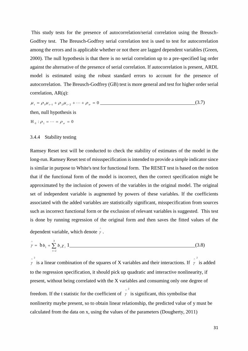
31
This study tests for the presence of autocorrelation/serial correlation using the Breusch-
Godfrey test. The Breusch-Godfrey serial correlation test is used to test for autocorrelation
among the errors and is applicable whether or not there are lagged dependent variables (Green,
2000). The null hypothesis is that there is no serial correlation up to a pre-specified lag order
against the alternative of the presence of serial correlation. If autocorrelation is present, ARDL
model is estimated using the robust standard errors to account for the presence of
autocorrelation. The Breusch-Godfrey (GB) test is more general and test for higher order serial
correlation, AR(q):
02211
ttt
(3.7)
then, null hypothesis is
0:10
3.4.4 Stability testing
Ramsey Reset test will be conducted to check the stability of estimates of the model in the
long-run. Ramsey Reset test of missspecification is intended to provide a simple indicator since
is similar in purpose to White's test for functional form. The RESET test is based on the notion
that if the functional form of the model is incorrect, then the correct specification might be
approximated by the inclusion of powers of the variables in the original model. The original
set of independent variable is augmented by powers of these variables. If the coefficients
associated with the added variables are statistically significant, misspecification from sources
such as incorrect functional form or the exclusion of relevant variables is suggested. This test
is done by running regression of the original form and then saves the fitted values of the
dependent variable, which denote
.
b
k
i
iibb
2
1 1 (3.8)
2
is a linear combination of the squares of X variables and their interactions. If
2
is added
to the regression specification, it should pick up quadratic and interactive nonlinearity, if
present, without being correlated with the X variables and consuming only one degree of
freedom. If the t statistic for the coefficient of
2
is significant, this symbolise that
nonlinerity maybe present, so to obtain linear relationship, the predicted value of y must be
calculated from the data on x, using the values of the parameters (Dougherty, 2011)

32
3.4.5 Error Correction Model (ECM)
An ECM has two important points: the study starts by estimating short-run coefficients and
then provide feedback or the speed of adjustment whereby short-run dynamics converge to the
long-run equilibrium path in the model. This study also develops the error correction model
(ECM) in order to test for the speed of adjustment and how the variables in the data set converge
towards equilibrium in the long run. Therefore, the ARDL version of the ECM for international
trade on economic growth is presented so as to check the speed of the error term towards
equilibrium. The sign of the error correction (EC) coefficient must be negative and significant
to ensure convergence of the dynamics of the long-run equilibrium. According to Dougherty
(2011) the model of the error correction model can be obtained as follows:
ttttt
31
1
43
2
1
211
)1( (3.9)
The model states that the change in Y in any period will be governed by the change in X.
3.5 Summary
A quarterly time series data was collected from 2000Q1 to 2017Q1 to help the researcher to
determine the relationship between international trade and economic growth in South Africa.
ADF, PP and DF-GLS were used to test if the variables are stationary or non-stationary. After
running stationarity test some variables were I(0) and others I(1) which lead to the adoption of
ARDL bounds test.

33
CHAPTER 4
DISCUSSION / PRESENTATION / INTERPRETATION OF FINDINGS
4.1 Introduction
This chapter presents the empirical results of all the tests outlined in previous chapter. There are some
levels of contradictions about the impact of international trade on economic growth. These
contradictions might be because of the differences in approaches and the compositions of data
and also the methodologies applied through the studies. Once international trade become fully
effective in South Africa trade will be affected in a positive or negative way. This study is
therefore envisaged to contribute to the growth policy making process in terms of
understanding how to maintain growth and the benefits of international trade liberalization.
The findings of data collected in previous chapter will clarify South Africa level on
international trade and economic growth.
4.2 Empirical tests results
This section presents the results of unit root tests the ARDL bounds test, the diagnostic and stability
tests.
4.2.1 Stationarity/Unit root tests results
4.2.1.1 Visual inspection
According to graphical presentation in figure 4.1, GDP seems to be non-stationary at level
because of the upwards trending movement over time. It gives the impression that economic
growth movement is controlled by time over the years (2000 – 2016). On the other hand,
figure 4.2 indicates that GDP seems to be stationary at first difference between the years 2000
to 2016. This is based on the oscillation around the mean of zero.

34
6.28
6.32
6.36
6.40
6.44
6.48
6.52
2000 2002 2004 2006 2008 2010 2012 2014 2016
LGDP
-.012
-.008
-.004
.000
.004
.008
.012
2000 2002 2004 2006 2008 2010 2012 2014 2016
Differenced LGDP
Figure 4.1 GDP at level difference Figure 4.2 GDP at 1st difference
Source: Authors estimations
4.2.1.2 Formal unit root tests results
The unit root tests were performed at intercept, trend and intercept models to determine
stationarity. The results are presented in Tables 4.1 to 4.12
Table 4.1: ADF test results at level
Variables
Model
specification
T-
statistics
Critical values Conclusion 1% 5% 10%
LGDP Intercept -1,905437 -3,530030 -2,904848 -2,589907 Non-stationarity I(0)
Trend &
intercept
-0,282102 -4,098741 -3,477275 -3,166190 Non-stationarity I(0)
EXCH Intercept -
7,282589***
-3,530030 -2,904848 -2,589907 Stationarity I(0)
Trend &
intercept
-
7,226035***
-4,098742 -3,477275 -3,166190 Stationarity I(0)
LEXP Intercept -1,469571 -3,536587 -2,907660 -2,591396 Non-stationarity I(0)
Trend &
intercept
-2,836769 -4,107947 -3,481595 -3,168695 Non-stationarity I(0)
LIMP Intercept -1,336194 -1,530030 -2,904848 -2,589907 Non-stationarity I(0)
Trend &
intercept
-2,393541 -4,098741 -3,477275 -3,166190 Non-stationarity I(0)
***0.01, **0.05, *0.10 significant level
Note: I (1) indicates unit root at first difference being stationary
I (0) indicates unit root in level being stationary
L indicates the logged variables
** indicates critical value at 5% level of significance
Source: Authors estimations
In table 4.1 exchange rate is stationary at level I(0) and some variables are non-stationary at
level and stationary at 1st different I(1).

35
Table 4.2: ADF test results at 1st difference
Variables
Model
specification T-statistics
Critical values Conclusion
1% 5% 10%
LGDP Intercept -6,453890*** -3,531592 -2,905519 -2,590262 Stationarity I(1)
Trend &
intercept
-6,750389*** -4,100935 -3,478305 -3,166788 Stationarity I(1)
LEXP Intercept -3,730950*** -3,536587 -2,907660 -2,591396 Stationarity I(1)
Trend &
intercept
-3,703980** -4,107947 -3,481595 -3,168695 Stationarity I(1)
LIMP Intercept -3,222882*** -3,536587 -2,907660 -2,591396 Stationarity I(1)
Trend &
intercept
-3,293051*** -4,107947 -3,481595 -3,168695 Stationarity I(1)
***0.01, **0.05, *0.10 significant level
Note: I (1) indicates unit root at first difference being stationary
I (0) indicates unit root in level being stationary
Indicate changes in first difference
L indicates the logged variables ** indicates critical value at 5% level of significance
Source: Authors estimations
In table 4.2: GDP, export and import are stationary at I(1) after first difference.
Table 4.3: Phillips - Perron test results at level
Variables
Model
specification T-statistics
Critical values Conclusion
1% 5% 10%
LGDP Intercept -1,586992 -3,530030 -2,904848 -2,58990 Non-stationarity I(0)
Trend &
intercept
-0,843730* -4,098741 -3,477275 -3,166190 Non-stationarity I(0)
EXCH Intercept -7,255711*** -3,530030 -2,904848 -2,589907 Stationarity I(0)
Trend &
intercept
-7,196922*** -4,098741 -3,477275 -3,166190 Stationarity I(0)
LEXP Intercept -1,888582 -3,530030 -2,904848 -2,589907 Non-stationarity I(0)
Trend &
intercept
-3,878191 -4,098741 -3,477275 -3,166190 Stationarity I(0)
LIMP Intercept -1,288125 -3,530030 -2,904848 -2,599907 Non-stationarity I(0)
Trend &
intercept
-2,501771 -4,098741 -3,477275 -3,166190 Non-stationarity I(0)
***0.01, **0.05, *0.10 significant level
Note: I (1) indicates unit root at first difference being stationary
I (0) indicates unit root in level being stationary
L indicates the logged variables ** indicates critical value at 5% level of significance
Source: Authors estimations

36
In table 4.3 exchange rate and log export under trend and intercept are stationary at level I (0)
at 5%.
Table 4.4: Phillips - Perron test results at 1st difference Variables Model
specification
T-statistics Critical values Conclusion
1% 5% 10%
LGDP Intercept -6,695452*** -3,531592 -2,905519 -2,590262 Stationarity I(1)
Trend & intercept -6,932077*** -4,100935 -3,478305 -3,166788 Stationarity I(1)
LEXP Intercept -16,68729*** -3,531592 -2,905519 -2,590262 Stationarity I(1)
Trend & intercept -18,77689*** -4,100935 -3,478305 -3,166788 Stationarity I(1)
LIMP Intercept -9,190217*** -3,531592 -2,905519 -2,590262 Stationarity I(1)
Trend & intercept -10,19689*** -4,100935 -3,478305 -3,166788 Stationarity I(1)
***0.01, **0.05, *0.10 significant level
Note: I (1) indicates unit root at first difference being stationary
I (0) indicates unit root in level being stationary
Indicate changes in first difference
L indicates the logged variables
** indicates critical value at 5% level of significance
Source: Authors estimations
Table 4.4: Shows that GDP, export and import are stationary at I(1) after first differencing. PP
tests support the ADF tests that all the logged variables are stationary at first difference I(1).
Table 4.5: DF-GLS test results at level
Variables
Model
specification T-statistics
Critical values
Conclusion
1% 5% 10%
LGDP Intercept 0,337636 -2,600471 -1,945823 -1,613589 Non-stationarity I(0)
Trend &
intercept
-0,947632 -3,709200 -3,138800 -2,842000 Non-stationarity I(0)
EXCH Intercept -6,466432*** -2,599413 -1,945669 -1,613677 Stationarity I(0)
Trend &
intercept
-7,067557*** -3,701600 -3,132400 -2,836000 Stationarity I(0)
LEXP Intercept -0,422211 -2,601596 -1,945987 -1,613496 Non-stationarity I(0)
Trend &
intercept
-2,745379 -3,716800 -3,145200 -2,848000 Non-stationarity I(0)
LIMP Intercept -0,100778 -2,599413 -1,945669 -1,613677 Non-stationarity I(0)

37
Trend &
intercept
-1,845598 -3,701600 -3,132400 -2,836000 Non-stationarity I(0)
***0.01, **0.05, *0.10 significant level
Note: I (1) indicates unit root at first difference being stationary
I (0) indicates unit root in level being stationary
L indicates the logged variables ** indicates critical value at 5% level of significance
Source: Authors estimations
Table 4.5: emphasis that the test on ADF, PP are correct because even in DF-GLS test exchange
rate is stationary at unit root level at 5% I(0).
Table 4.6: DF-GLS test results at 1st difference
Variables
Model
specification T-statistics
Critical values
Conclusion 1% 5% 10%
LGDP Intercept -3,761202*** -2,600471 -1,945823 -1,613589 Stationarity I(1)
Trend &
intercept
-6,683496*** -3,705400 -3,135600 -2,839000 Stationarity I(1)
LEXP Intercept -2,657457*** -2,601596 -1,945987 -1,613496 Stationarity I(1)
Trend &
intercept
-3,406301*** -3,716800 -3,145200 -2,848000 Stationarity I(1)
LIMP Intercept -3,053658*** -2,601596 -1,945987 -1,613496 Stationarity I(1)
Trend &
intercept
-3,225863*** -3,716800 -3,145200 -2,848000 Stationarity I(1)
***0.01, **0.05, *0.10 significant level
Note: I (1) indicates unit root at first difference being stationary
I (0) indicates unit root in level being stationary
Indicate changes in first difference
L indicates the logged variables
** indicates critical value at 5% level of significance
Source: Authors estimations
Table 4.6: back-up the results of unit root done by ADF, PP that symbolises that indeed GDP,
export and import are stationary at first difference I(1). In detail the results for the unit root test
are presented in appendix A. The results of the three tests indicate that some of the series are
found to be non-stationary; however, the first differences of these series lead to stationarity.
4.2.2 Bounds test results
Table 4.7 and Table 4.8 present results of the bounds testing approach. In detail the results for
the Bounds test are presented in appendix B. E-views 9 automatically selects the optimal lag

38
length of our model using the Akaike Information Criterion (AIC) and for this study a lag
length of 6 was selected to accommodate the variables in question.
Table 4.7 Bounds test results
Equation F-statistic Lower bound I(0)
@ 5%
Upper bound I(1)
@ 5%
Results/
Outcome
Economic growth 5.02 2.79 3.67 Cointegrated
Source: Authors estimations
According to Persaran et al., (2001) significant levels for lower bound and upper bound are
shown as follows hereafter:
Table 4.8: Significant levels for lower bound and upper bound
Significant level I(0) or Lower bound I(1) or Upper bound
10% 3.65 4.66
5% 2.79 3.67
1% 2.37 3.20
Persaran et al., (2001)
The number of independent variables in this model is 3, hence k=3. All the lower bound and
upper bound critical values are obtained from (Pesaran et al., 2001). The calculated F-statistic
= 5.02 and is greater than the lower bound critical value of 2.79 and the upper bound critical
value of 3.67 at 5% level of significance, therefore this symbolise the presence of cointegration
among the variables.
The bound testing approach has provided enough evidence of a long-run relationship between
all the variables on economic growth model, the study then proceeds to estimate the long-run
coefficients of the model. The calculated results show that F statistics exceeds the upper bound;
the null hypothesis of no cointegration can be rejected. Estimating the long-run coefficients
and the ECM along with the short-run parameters become necessary.
4.2.3 ARDL long-run coefficients model
Table 4.9: ARDL long-run coefficients
Variables Coefficients
EXCR 0.000014
LEXP -0.391893
LIMP 0.578821
C 5.315750
Source: Authors estimations

39
Table 4.9 presents the summary of the results of the long-run ARDL model for the international
trade equation and all the details are in appendix C. All the variables in the model exert
significant long-term influences on the economic growth. EXCH with a coefficient of 0.00%
indicates a positive long-run relationship between the EXCH and economic growth. This
suggests that a 1% appreciation of the exchange rate will lead to 0.00% improvement or
increase on economic growth. South Africa exchange rate is significant. This result is also
consistent with economic theory. A competitive exchange rate is seen as an esential ingredient
of dynamic growth and employment in developing countries. It allows domestic firms to
benefit from rapid growth in international trade and attracts international firms searching for
the best location for sourcing of their goods. This may also have positive spill over’s for
domestic technological development, which might lead to a process of learning how to produce
with the best technologies available, and with the best marketing tools for the global economy
(Spiegel, 2007).
Export stands at -0.361, suggesting a negative relationship between LEXP and LGDP in the
long-run. Export has no significant effect output in the long-run. A 10% increase in export will
lead to 3.61% deterioration in the level of the economic growth. The coefficient of LEXP is
negative and statistically not significant at 5 per cent level of confidence with a value of -0.361.
This implies that at 1% increase in the degree of export would lead to about 0.361 decreases in
economic growth (GDP) of South Africa. Export does not lead to economic growth in South
Africa. If the country exports more, economic growth will decrease since South Africa like
other developing countries relies much on homogeneous agricultural products, which some are
harvested seasonally and also depend on climate change. No rains-no crops, results will be poor
production on farms, livestock dies of drought and increase in food prices of home produce.
Although South Africa also exports some commodities such as minerals, iron, steel, vessels,
wood, plastic and rubber still the economic growth is unstable.
In this study, export impact growth negatively because South Africa is importing much from
its bilateral countries and export little. The other reason is that for South Africa, endowments
of natural resources or basic industries are no longer necessary or sufficient for participation in
this new global environment. South Africa focus on producing lot of agricultural commodities
that fail to compete in the global market. On the other hand, South Africa export is weak
because as the country is advancing or reaching maturity its agricultural sector demand

40
decreases and the focus shift to other performing sector. Another reason is that South Africa
prices are not stable and its trading partners always search for better trading partners.
The results presented in this study are similar to Flattrs and Stern (2007), that highlighted that
rising exports of resources in South Africa have led to appreciation of the rand. A stronger rand
against major currencies could contribute to the declining competiveness of South Africa’s
exports. Meaning that some countries can withdraw exporting from South African and while
South Africa do the same our economic growth remain on the same level and did not grow. In
the same vein, Kehinde et.al, (2012) concluded that higher level of trade restrictions has been
a huge obstacle to export and growth performance in developing countries like South Africa.
The results are also consistent with the Heckscher – Ohlin theory which focuses on the
differences in relative factors endowments and factors prices between nations as the most
determinants of trade. The model identified difference in pre-trade product prices between
nations as the basis for trade. The theory assumed two countries, two commodities and two
factors. There is perfect competition in both factor and product market. It assumed that factor
inputs; labour and capital in the two countries are homogeneous. Production function also
exhibits constant return to scale because the production situation increases exactly in the same
proportion which factor production increases. Production possibility curve is concave to the
origin. The model suggests that the less develop countries that are labour abundant should
specialize in the production of primary products especially agricultural product because the
labour requirement of agricultural is high except in the mechanized form of farming (Usman,
2011).
Import stands at 0.578, suggesting a positive relationship between LIMP and LGDP in the
long-run. A 10% increase in import will lead to 5.78% improvement in the level of economic
growth. The coefficients of import are 0.57 and highly significant suggesting that GDP rises
by 57 per cent of the increase in the long-run. South Africa imports have impact on economic
growth is sustained by higher level of import and little export. Omoju and Adesanya (2012)
find out that exports, imports and exchange rate have a significant positive impact on economic
growth in developing countries. Empirically, there appears to be good evidence that
international trade affects economic growth positively by facilitating capital accumulation,
industrial structure upgrading, technological progress and institutional advancement. The result
is also consistent with economic theory and more specifically, increased imports of capital and

41
intermediate products, which are not available in the domestic market, can result in the rise in
productivity of manufacturing (Lee 1995).
Table 4.10: Error Correction Model
Variables Coefficients Standard error T-statistic
EXCH 0.000002 0.000062 0.021681
LEXP(-1) 0.084169 0.021041 4.000230
LIMP(-1) -0.023217 0.023491 -0.408162
CointEq(-1) -0.125246 0.038971 -3.213864
Indicate changes in first difference
CointEq equals to the size of the error correction model
L indicates the logged variables
Source: Authors estimations
The results of the error-correction model are quite consistent between long-run and short-run.
The short-run impact of EXCH on GDP is positive and significant at 5 per cent level of
significance. Exchange rate and Import foster GDP growth in South Africa both in the short-
run and long-run. The role of export in the error-correction model remains as insignificant as
before or in short-run and long-run. The error-correction model is negative as expected but it
is significant at 10 per cent level of significant instead of the conventional 5 per cent level.
The negative sign before the error-correction term, -0.125 suggests that the long-run
equilibrium relation comes back to the speed of adjustment. The value of the coefficient
however is very low, which suggests that it will take long time to restore steady-state or speed
of adjustment if the system is distributed. The estimated model shows a fair level of goodness
of fit.

42
4.2.4 Diagnostic tests results
Figure 4.3: Normality test results
0
2
4
6
8
10
12
14
-0.006 -0.004 -0.002 0.000 0.002 0.004
Series: ResidualsSample 2001Q2 2017Q1Observations 64
Mean -1.29e-15Median 6.68e-05Maximum 0.004544Minimum -0.005678Std. Dev. 0.002111Skewness -0.145106Kurtosis 3.078125
Jarque-Bera 0.240872Probability 0.886534
The residuals are normally distributed in the model as shown by not rejecting the null
hypothesis of the Jarque-Bera test. The p-value is greater than 5 per cent; therefore the study
cannot reject the null hypothesis because at 8.86% probability is normally distributed. If P
value is less than 5 per cent the study cannot accept the null hypothesis and accept the
alternative, meaning that the x value is not normal. The skewness and the kurtosis rely on the
probability value. The bell shape of the histogram shows that the residuals are normally
distributed.
Table 4.11: Diagnostic checks on the error term
Test Null Hypothesis Test
Statistic
P-Value Conclusion
Jarque-Bera Residuals are
normally
distributed
0.240872 0.886534 Do not reject H0 as P-value is
greater than level of
significance at 5%, therefore
the residuals of the model are
normally distributed.
Breusch-
Pagan-
Godfrey
No Serial
correlation
1.851886 0.3962 Do not reject H0 as P-value is
greater than level of
significance at 5%, therefore
there is no serial correlation.
Breusch-
Pagan-
Godfrey
No
heteroskedasticity
9.139524 0.6090 Do not reject H0 as P-value is
greater than level of
significance at 5%, therefore,
no heteroskedasticity in the
model, but there is
homoscedasticity which is
desirable.

43
Harvey No
heteroskedasticity 10.02451 0.5282 Do not reject H0 as P-value is
greater than level of
significance at 5%, therefore,
no heteroskedasticity in the
model, but there is
homoscedasticity which is
desirable. Glejser No
heteroskedasticity 9.495565 0.5762 Do not reject H0 as P-value is
greater than level of
significance at 5%, therefore,
no heteroskedasticity in the
model, but there is
homoscedasticity which is
desirable. Arch No
heteroskedasticity 0.219560 0.6394 Do not reject H0 as P-value is
greater than L.O.S at 5%,
therefore, no heteroskedasticity
in the model, but there is
homoscedasticity which is
desirable. Null hypothesis: Homoskedacicity Alternative hypothesis: Heteroskedasticity
Source: Authors estimations
If the model has heteroskedasticity, we reject the null (homoskedacicity) and accept the
alternative. Table 4.11 presents the residual diagnostic of the economic growth model.
Detailed results for all the diagnostic tests are presented in Appendix D. The study tested for
serial correlation using the Breusch-Godfrey test. The test reports the F-statistic with a value
of 1.85 and a P-value of 0.39 implying that the study fails to reject the null hypothesis of no
serial correlation at all conventional level of significance. Breusch-Pagan-Godfrey test for
heteroskedasticity has LM statistic with a value of 9.13 and a P-value of 0.60 implying that the
LM statistic is insignificant at 5% level of significant. Therefore, failing to reject the null
hypothesis of constant variance and concluding that heteroskedasticity is not present in the
data. The study also tested for Arch effects using the Arch test. The test reports an LM statistic
with a value of 0.21 and a P-value of 0.63 implying that the null hypothesis of no Arch effects
in the data is rejected. Last0ly, according to Harvey and Glejser the model has no
heteroskedasticity as all their P-values are greater than level of significant at 5%. From the
results of diagnostic tests, this study estimated model is free of serial correlations,
misspecification errors, and heteroskedasticity at the 5 per cent level of significance.

44
4.2.5 Stability tests results
Table 4.12: Ramsey Reset tests results
Test H0 T-statistic P-value Conclusion
Ramsey Reset The model is
correctly specified
0.133163 0.8946 Do not reject H0 because the
P-value is greater than the
level of significant at 5%.
Source: Authors estimations
Table 4.12 reports the results from the Ramsey Reset test. Detailed results for the Ramsey
Reset test are presented in Appendix E. Null hypothesis states that the model is correctly
specified. The P-value is greater than the level of significant at 5%, the null hypothesis is not
rejected, and therefore, the model of economic growth is correctly specified.
4.3 Summary
This chapter sum-up the results of the study based on the methodology discussed in chapter 3.
Firstly, the time series quarterly data were discussed to visually check the stationarity of the
variables with ADF; in addition, PP and DF-GLS unit root test were used as supporting
evidence. Secondly, the ARDL bounds test was adopted to check short-run and long-run
cointegration in the model. Lastly, the diagnostic and stability test conclude the chapter.

45
CHAPTER 5
SUMMARY, RECOMMENDATIONS, CONCLUSION
5.1 Introduction
This chapter presents the summary and interpretation of the findings of the study, conclusions,
and contributions of the study and limitations of the study.
5.2 Summary and Interpretation of Findings
The study analysed the effect of international trade on economic growth in South Africa with
the aim of addressing three objectives. The first objective was to examine the relationship
between international trade and economic growth. The second one was to examine the
relationship between international trade and exchange rate and the last one examined the
relationship between international trade and export.
The ARDL bounds test was employed to analyse the effects of international trade on economic
growth in South Africa and Belloumi (2014)’s model was used as the basis for the formulation
of the model and The data was sourced from South African Reserve Bank (SARB) and
Quantec. The ADF, PP and DF-GLS analytic technique were performed to test stationarity and
the ARDL model was employed in data analysis to help address the objectives that the study
intended to address. The study found that exchange rate and import were the main determinants
of economic growth in the long-run in South Africa. Furthermore, the study found out that
the coefficient of export had negative relationship to economic growth it is not significant in
the long-run.
5.3 Conclusions
The study found out that gross domestic product, exchange rate and export were the important
variables in explaining variations in economic growth in South Africa. The other factors like
exports that were sought to be determinants of growth in South Africa turned out not to be
contrary to what most empirical studies suggested. This means that South African economic
growth is unique in its activities domestically and abroad. The study makes it clear that there
is over reliability to other countries done by South African economy. The study examines the

46
effect of international trade on economic growth in South Africa. The results show that
exchange rate and import are positively related to GDP, while export has a negative influence
on GDP. These results are in line with Zahonongo (2017) who concluded that sub-saharan
African countries must productively control trade opennesss, particularly the import of
consumption goods, boosting their economic growth through international trade. At the same
time this result is in contrast with Eravwoke and Onokero (2012) who found out that export is
highly significant in South African economy. According to Biru (2014) testing export-led
growth in Bangladesh, imports donot have any significant relationship with GDP. The study
findings add a new dimension to the existing literature on the examines the effect of
international trade on economic growth in South Africa, also due to the fact that the findings
contradict the conclusions reached by the majority of the past studies.
5.4 Limitations of the study
There were some limitations experienced in relation to the availability of some data. Although
most of the quarterly data was readily available, some of the data did not cover second quarter
of 2017. The data had to be adjusted to Q1 2017 for the purpose of the study. There was no
delimitation experienced in this study.
5.5 Policy recommendations
The study empirical findings have a certain implication for policy discussions. Since the results show
that South African export have negative impact on growth, it is recommended that South African
government must promote trading of goods and services internally and not focus much on exporting its
primary goods and services abroad because it weakens the economy. Since we have noticed that South
African economic growth is unique in its activities domestically and abroad this must help us
reduce over reliability to other countries and boost our economy by implementing or pursuing
policy that promote growth such as focusing on the other sectors or promoting the use of
technology gadgets as most developed countries relies on that. It is recommended that South
African government must rely on the strength it have in order to strengthen its currency and
reduce importing poor quality product “fongkong” that is weakening the economy. It is
recommended that South Africa must produce or export according to the need of the industry,
so that the country benefit in return. Lastly, it is recommended that South Africa must support
local industries and firms to create more employment opportunities and start programmes that
will make youth to be active in businesses and reduce over reliance to the government.

47
6. REFERENCES
Adedeji, S. Writing and Research Proporsal in G.O.edu.ul.ng/so Adedeji. 2006.
Adeleye, J.O and O.S. and Adewuyi, M.O Adeteye. “Impact of International Trade on Economic
Growth in Nigeria.” International Journal of Finance Research 6.3 (2015): 163.
Adubi, A.A. Price, Exchange Rate Volatility and Nigeria's Agricultural Trade Flows; A Dynamic
Analysis, (NCEMA). Ibadan Nigeria: National Centre for Economic Management and
Administration, 1999.
Price, Exchange rtae volatility and Nigeria's Agricultural Trade flows; A dynamic Analysis (NCEMA).
Ibadan Nigeria: National Centre for Economic Management and Administration., 1999.
Afonso, O. The Impact of International Trade on Economic Growth. Vol. 6. FEP Working Papers, 2001.
Agama, L. "Trade Openness and Economic Growth: Empirical Evidence from Africa". Washington D.C.:
US International Trade Commission., 2001.
Ahmend, A.D, Cheng, E. and Messinis, G. The Role of Exports, FDI and Imports in Development: New
Evidence from Sub-Saharan African Countries. Melbourne: Center for Strategic Economic
Studies, Victoria University., 2008.
Akpan, E.O. and Atan, J.A. “"Effects of Exchange rate Movement on Economic Growth in Nigeria".”
CBN Journal of Applies Statistics 2.21 (2012).
“Effects of Exchange Rate Movement on Economic Growth in Nigeria.” CBN JournaL of Applies
Statistics 2.21 (2012).
Angomoko, B.B. The Effect of Chinese Economic Growth on South Africa's Exports to China. Submitted
in accordance with the requirements for the degree of Master of Commerce in the subject
Economics. University of South Africa, 2017.
The effects of Chinese economic growth on South Africa's export to China. University of South africa,
2017.
Anwer, S.M. and Sampath, R.K. Exports and Economic Growth: Western Agricultural Economics
Association. Nevada, Sparks/Reno, 1997.
Asterious, D. and Halls,S. Applied Econometrics: A Modern Approach. Palgrave: Macmillan, 2007.
Auer, R. and Fisher, A.M. The Effect of trade with low-income countries on US industry. Federal
Reserve Bank of Dallas. Globalisation and Monetary Policy Institute. Working paper no.14,
2008.
Bahmani, O.M. and Nimrod, F. “Openness and Economic Growth".An Empirical Investigation Applied
Economics. 6 (1991): 557-561.
Balassa, B.,. “Policy Responses to Exogenous Shocks in Developing Countries,.” American Economic
Review, 5 (1986): 75-78.

48
Balassa, D.,. “Exports and Economic Growth:Further Evidence,.” Journal of Development Economics.
5.2 (1978): 181-189.
Baldwin, R.,. “Openness and Growth: What's the Empirical Relationship?” 2003.
Belloumi, M. The Relationship between Trade, FDI and Economic Growth in Tunisia:An Application of
autoregressive distributed lag model. Sousse Tunisia: University of Soussse, 2014.
Bentzen, J and Engsted, T. A Revival of the ARDL Model in Estimating Energy Demand Relationship
(Cointegration: Bounds Testing Approah). Vol. 26. 2001.
Biru, P.P. “Testing Export-Led Growth in Bangladesh: An ARDL Bounds Test Approach.” International
Journal of Trade, Economics and Finance 5.1 (2014): 1-5.
Borenstein, De Gregorio, J. and Lee, J. “How does Foreign Direct Investment Affect Economic
Growth?” Journal of International Economics 45 (1998): 115-135.
Caves, R.E. "Multinational Enterprise and Economic Analysis". Ed. 2nd edition. Cambridge:
Cambridge University Press, 1996.
Coe, D.T. and Helpman, E. "International Research & Development Spillovers" European Economic
Review. NBER Working Paper, No.4444., 1995.
Coe, D.T. and Helpman, E. "International Research & Development Spillovers". New York: European
Economic Review, 1995.
Cooper, D.R., and Schindler, P.S.,. Business Research Methods,. NY Mcgraw - Hill, 2003.
Davidson, R. and MacKinnon, J.G. Econometric Theory and Methods. New York: Oxford University
Press, 2004.
Davies, R. A South African Trade Policy and strategy Framework. Pretoria: Prepared by the
International Trade and Economic Development Division of the Department of Trade and
Industry South Africa., 2010.
A South African Trade Policy and Strategy Framework May 2010. Pretoria, Sunnyside.: Prepared by
the International Trade and Economic Development Division of the Department of Trade and
Industry South Africa., 2010.
De Melo, J.C.M and Panagariya, A. "Regional Integration Old and New". Working Paper Series 985.
World Bank., 1992.
Deumal, M. and Ozyurt, S. “Impact of International Trade Flows on Economic Growth in Brazil State.”
Review of Economics and Institutions. 2.1 (2011).
Dlamini, S. Bank credit extension to the private sector and inflation in South Africa. Grahamstown:
Rhodes University (Thesis-Masters), 2008.
Dollar, D. and Kraay, A.,. “Growth is Good for the Poor,.” Journal of Economic Growth, 7 (2000): 195-
225.

49
Dolllar, D.,. “Outward-Oriented Developing Economies Really do Growth Mor Rapidly,.” Economic
Development and Cultural Change, 40.3 (1992): 523-544.
Dougherty, C. Introduction to Econometrics. Fourth Edition. New York: Oxford University Press, 2011.
Du Plessis, S. Economic Growth in South Africa since 1994. Department of economics and Bureau of
economic research., 2014.
Durlauf, S. Econometric Analysis and the study of economic Growth: A Sceptical Perspective. In
Macroeconomics and the Real World. Oxford University Press., 2000.
Easterly, W., and Rebelo, S. “Fiscal Policy and Economic Growth: An Empirical Investigation.” Journal
of Monetary Economics 32 (1993): 417-458.
Edwards, L. and Lawrence, R. South African trade policy matters: Trade performance and trade
policy. CID Working paper No 135. USA: Centre of International Development at Havard
University, 2006.
Edwards, S. “Openness, Trade Liberalization, and Growth in Developing Countries.” Journal of
Economics 31.3 (1993): 1358-1393.
Elliot, G., Rothenberg, T and Stock, J. “'Efficient tests for an autoregressive unit root'.” Econometrica.
64.4 (1996): 813-836.
Eravwoke, K.E. and Oyivwi, D.O. “Growth Perspective via Trade in Nigeria: A Cointehration Approach,
African Research Review". An International Multidisciplinary Journal, Ethiopia 6.1 (2012): 18-
26.
Ezike, J.E, Ikpesu, F and Amah, P. “Macroeconomic Impact of Trade on Nigerian Growth: An Empirical
Evaluation.” Research Journal of Business Management and Accounting, 1.4 (2012): 079-083.
Flattrs, F. and Stern, M. Trade and trade policy in South Africa: Recent trends and future prospects.
Development Network Africa, 2007.
Fourie, F. and Philippe,B. How to Think and Reason in Macroeconomics. Juta & Co Ltd., 2009.
Frankel, J.A and Romer, D. “"Does Trade Cause Growth?".” American Economic Review, 89 (1999):
379-399.
Gou, H.F., Cheng, K. and Dong, H. Epidermal Growth Factor Receptor (EGFR)- RAS Signaling Pathway
in Penile Squamous Cell Carcinoma. China: https//doi.org/10.1371/journal.pone.0062175,
2013.
Green, W. Econometric Analysis (4th edition). Englewood Cliffs, New Jersey: Prentice Hall., 2000.
Greenaway, D. and Sapsford, D.,. 'What does Liberalisation Do for Exports and Growth?',. Vol. 130.
WeltwirtschaftlichesArchiv,, 1994.
Greenaway, D., Leybourne, S.J., and Sapsford, D.,. 'Modelling Growth and Liberalisation: Using
Smooth Transition Analysis',. Vol. 35. Economic Inquiry, 1997.

50
Grossman, G.M and Helpman, E. Innovation and Growth in the Global Economy. Cambridge, MA: MIT
Press, 1991.
Gujarati, D. Basic Econometrics. Ed. fouth edition. 2004.
Hamilton, D. Time Series Analysis- Princenton:. University Press, 1994.
Hofman, P. The Impact of International Trade and Foreign Direct Investment on Economic Growth
and Technological changes. Springer- Verlag Berlin Heidelberg., 2013.
Hossain, S. Econometrics Modelling, Frequently asked questions. multimedia university 63100
cyberjaya, www.sayedhossain.com, 2008.
Italianer, A. "Wither the Gains from European Economic Integration". Revue Economique., 1994.
Ito, T. Exchange Rate Movements and their Impact on Trade and Investment in the APEC Region.
Washing D.C.: International Monetary Fund Publication Servicess., 1996.
Jenkins, R. and Sewn, K. “International Trade and manufacturing Employment in the South: Four
country case studies.” International Development Centre 34.3 (2006): 299-322.
Johansen, S and Juselius, K. "Maximum Likelihood Estimation and Inference on Cointegration- with
Application to the Demand for Money". Vol. 52. Oxford Bulletin of Economics and Statistics,,
1990.
Johnsson, G. and Subramanian, A. Dynamic Gains from Trade: Evidence from South Africa.
Washington D.C.: International Monetary Fund Working Papaer 145., 2000.
Jude, C and Pop Silaghi, M.L. "Some Determinants of Economic Growth in Romania: Foreign trade
and Foreign Direct Investments". Romania: ISSN: 1582-5450, 2008.
Kamin, S.B. and Klan, M. "Some Multi-Counting Evidence on the Effect of Real Exchange rates on
Output". Washington D.C.: International Finance Discussion Paper no.611, 1998.
Kamin, S.B. and Marl, K. “Some Multi-Counting Evidence on the Effect of Real Exchange Rates on
Output.” International Finance Discussion Papers No.611. Washington D.C.: Federal Reserve
Board, 1998.
Kandil, M. “"Exchange rate Fluctuations and Economic activity in Developing Countries: Theory and
Evidence".” Journal of Economic Development 29.1 (2004): 15.
“Exchange Rate Fluctuations and Economic Activity in Developing Countries: Theory and Evidence.”
Journal of Economic Development 29.1 (2004).
Kavoussi, R.M. “Export Expansion and Economic Growth". Development Economics 14.1 (1984): 241-
250.
Kehinde, O., Adekunjo, O., Olufemi, E. and Kayode, K. “Foreign Trade and Economic Growth in
Nigeria: An Empirical Analysis.IOSR .” Journal of Humanities and Social Science (JHSS) 2.1
(2012): 73-80.

51
Keshab, R.B and Armah, M.K. The Effects of Exchange Rate on the Trade Balance in Ghana: Evidence
from Cointegration Analysis,. United Kingdom: Centre for Economic Policy, Business School,
University of Hull, 2005.
Khothari, R.,. Research Methodology: Methods and Techniques. New Delhi-India.: New Age
International, 2004.
Kingori, B.M. An Analysis of the determinants of Private Sector investment in Kenya using the
Autoregressive Distributed Lag (ARDL) Approach : A thesis For Masters of Science in
Economics. Namibia: University of Namibia, 2015.
Kojima, K., and Osawa, T. “"Micro and Macro-Economic Models of Foreign Direct Investment".”
Journal of Economics (1984).
Krueger, A.O.,. “'Trade Policy and Economic Development: How we Learn',.” American Economic
Review. 87 (1997): 1-22.
Kruger, A.O.,. “Foreign Trade Regimes and Economic Liberalisation.” The Economic Journal. (1978).
“Why Trade Liberalisation is Good for Growth.” The Economic Journal 108 (1998): 1513-1522.
Krugman, P. and Helpman, E. Imperfect Competition and International Trade: Evidence from
Fourteen Industrial Countries. Camnridge: Harvard University Press, 1988.
Krugman, P., Maurice, O. and Melitjz, M. International Economics Theory and Policy. Pearson, 2012.
Kumar, V.,. “"Developing Credit Bureau IFC's Effort" It is not just Technology: Planet Finance
Opportunities and Challenges, Micro Finance Focus.” Journal of Applied Economics, 5.2
(2009): 123-129.
Lall, S. Foreign Direct Investment, Technology Development and Competitiveness: Issues and
Evidence. Monograph, 2000.
Lee, J.W. “Capital Goods Import and Long-run Growth",. Development Economics, 48.1 (1995): 91-
110.
Lin, S.,. “Foreign Trade and China's Development: A Time Series Analysis,.” Journal of Economic
Development, 25.1 (2000): 145-153.
Lopez, R.A. “Trade and Growth: Reconciling the Macroeconomic and Microeconomic Evidence.”
Journal of Economic Surveys, 19.4 (2005): 623-647.
Maggiora, D.D. and Skerman, R. Johansen Cointegration analysis of American and European stock
Market indices: An Empirical study. United States: Lund University, Masters thesis in finance.
, 2009.
Maitena, D. and Banco, de Espana. Definitions of Foreign Direct Investment (FDI) a Methodological
note. [email protected]., 2013.
Maizels, A. Industrial Growth and World Trade. United Kingdom: Cambridge University Press., 1963.

52
Mankiw, G. Principles of Macroeconomics. Thomson South Western, 2011.
Marshall, A. Principles of Economics. London: Macmillan, 8st ed., 1920, 1890.
Mattoo, A., Rathindran, R. and Subramanian, A. Measuring Services Trade Liberalisation and its
Impact on Economic Growth:. Washington DC.: World Bank, 2001.
Melina, D. and D. and Antonios, A. Chaido. A Causal Relationship between Trade, FDI and Economic
Growth for Greece. Greece: Macedonia University Press, 2004.
Mill, J.S. Principles of Political Economy. Longmans, Green and Co., 1848.
Mogoe, S. The Impact of International Trade on Economic Growth in South Africa: An Econometrics
Analysis. The Research Project Submitted in partial fulfilment of requirement for a Masters
Degree in Economics in the faculty of Commerce and Administration. Mafikeng: North West
University, 2013.
Mohr, P. and Fourie,L. Economics for South African Students. Pretoria: Van Schaik, 2008.
Moudatsou, A. “Foreign Direct Investment and Economic Growth in the European Union.” Journal of
Economic Integration 18.4 (2003): 689-707.
Nageri, K. I. Olodo A. O. Bukulo, H. and Babatunde, A. M. “"An Empirical study of Growth through
Trade: Nigeria Evidence".” Arabian Journal of Business and Management Review (OMAN
chapter). 3.5 (2013): 1-2.
Nageri, K.I., Olodo, A.O., Bukulo, H. and Babatunde, A.M. “"An Empirical study of Growth through
Trade: Nigerian Evidence".” Arabian Journal of Business and Management Review (OMAN
chapter) 3.5 (2013): 1-2.
Narayan, P.K. “The Saving and Investment Nexus for China: Evidence from Cointegration Tests.”
Applied Economics 37.17 (2005): 1979-1990.
Njikam, O. Exports and Economic Growth in sub-saharan Africa: Is there a connection. Ghana:
University of Yaounde, 2003.
Nzimakwe, T.I.,. “South Africa's NGOs and the quest for Development.” International NGO Journal .
3.5 (2008): 90-97.
Odhiambo, N.M. “Energy Consumption and Economic Growth in Tanzania: An ARDL bounds Testing
Approach.” Energy Policy Journal 37.2 (2009): 617-622.
Odoemena, I.U. “"Effects of Exchange Rate Fluctuations on Economic Growth of Nigeria".”
International Journal of Innovative Finance and Economics Research 4.2 (2016): 1-7.
—. “Effects of Exchange Rate Fluctuations on Economic Growth of Nigeria.” International Journal of
Innovative Finance and Economics Research 4.2 (2016): 1-7.
Omoju, O. and Adesanya, O. “Does Trade Promote Growth in Developing Countries? Empirical
Evidence from Nigeria". International Journal of Development and Sustainability. 1.3 (2012).

53
Opukri, C. and Edoumlekomu, E. “Economic Growth Factor in Nigeria: The Role of Global Trade.”
American Journal of Humanities and Social Sciences. 1.2 (2013): 51-55.
O'scar, A.,. The Impact of International Trade on Economic Growth. University of Birmingham, UK:
Faculty of Economics., 2001.
Pesaran, M., Shin, Y and Smith, R. “Bounds Testing Approaches to the Analysis of Level
Relationships”. Journal of Applied Econometrics. 16.3 (2001): 289-326.
Pesaran, M.H and Shin, Y. An Autoregressive Distributed Lag Modelling Approach to Cointegration
Analysis. Chapter 11 in Econometrics and Economic Theory in the 20th Century: The Ragnar
Frisch Centennial Symposiumm, Strom S (ed.). Cambidge: Cambridge University Press:, 1999.
Phillips, P.C.B., and Perron, P.,. "Testing for a Unit Root in Time Series Regression",. Vol. 75.
Biometrica, 1988.
Rajan, R.G and Zingales, L. “The Great Reversals: The Politics of Financial Development in the
Twentieth Century .” Journal of Financial Economics 69.1 (2003): 5-50.
Rankin, N. Exporting and eport dynamics among South African firms. Economic Diplomacy
Programme Occassional paper No 149. Johannesburg: South African Institute of Internal
Affairs., 2013.
Rodriguez, F. and Rodrik, D. “"Trade Policy and Economic Growth: A Skeptic's Guide to the
Crossnational Evidence, In: Bernanke B and Rogoff K.S. eds".” Macroeconomics Annual 2000.
Cambridge, MA: MIT Press for NBER, 2000. 261-324.
'Trade Policy and Economic Growth: A Skeptic's Guide to the Cross-National Evidence', National
Bureau of Economics. Washington, DC.: Center for Economic Policy Research, Discussion
Paper 2143., 1999.
Rodrik, D. The New Global Economy and Developing Countries: Making Openness Work. Washington
D.C.: Overseas Development Council., 1999.
Sachs, J.D. and Warner, A. Economic Reform and Process of Global Integration. Vol. 26(1). Brookings
Papers of Economic Activity, 1995.
Saggi, K.,. Trade, Foreign Direct Investment, and International Technology Transfer:. A Survey, World
Bank Policy Research Working Paper, 2000.
Samuelson, P.A. “International Factor Price Equalization once again.” Economic Journal 59 (1949):
181-197.
“International Trade and the Equalisation of Factor Prices.” Economic Journal 58 (1948): 163-184.
Schurink, W.J.,. Evaluating Qualitative Research. Johannesburg: University of Johannesburg., 2005.
Lectuerthirteen: Evaluating Qualitative Research. Johannesburg.: University of Johannesburg, 2005.
Sekuma, R. A study of Cointegration Models with Applications. University of South Africa, 2011.

54
Sj"o, Bo. Testing for Unit Root and Cointegration. 2008.
Smith, A. An Inquiry into the Nature and Causes of the Wealth of Nations. Libson, 1776.
An Inquiry into the Nature and Causes of the Wealth of Nations. Libson, 1776.
Solow, R. “A Contribution to the Theory of Economic Growth .” Quarterly Journal of Economics
(1956): 65-94.
Spiegel, S. National Development Strategies Policy Notes Macroeconomic and Growth Policies. New
York-United Nations: Department for Economic and Social Affairs (UNDESA), 2007.
Stern, M. and Flatt. Trade and Trade Policy in South Africa: Recent Trends and Future Prospects.
Development Network Afrca. South Africa: http://www.dnaeconomics.com/fileuploadsfile
063020080109 file 101820070217, 2007.
Sun, P. and Heshmati, A. International Trade and Its Effects on Economic Growth in China. China:
Discussion Paper no 5151, 2010.
Swan, T. W. “Economic Growth and Capital Accumulation.” Economic Record 32 (1956): 334-361.
Te Velde, D.W. “Government Policies for Inward Foreign Direct Investment in Developing Countries.”
United States: Implications for Human Capital Formation and Income Inequality, Paper
presented at OECD Development Centre on FDI and Human Capital., 2001.
Usman, O.A. “Performance Evaluation of Foreign Trade and Economic Growth in Nigeria.” Research
Journal of Finance and Accounting. 2.2 (2011): 2222-1697.
Vamvakidis, A. “Regional Integration and Economic Growth.". The World Bank Economic Review,
12.2 (1998).
Vickers, B. South Africa's Trade Policy and Strategy Framework. SA- Johannesburg: International
Trade and Economic Development (ITED) and Department of Trade and Industry (DTI), 2014.
Vijayasri, G.M. “the Importance of International Trade in the World". International Journal of
Marketing, Finance Services & Management Research 2.9 (2013): 2277-3622.
Winter, A.,. Trade Policies for Poverty Alleviation. In Hoekman, Bernard, Mattoo, Aadiya and English,
Phillip (eds). Washington DC: Development, Trade and WTO, A Handbook. World Bank, 2002.
Young, A. “Increasing Returns and Economic Progress.” Economic Journal 38 (1928): 527-542.
Zahonongo, P. “Trade and Economic Growth in Developing Countries: Evidence from Sub-saharan
Africa.” Journal of African Trade (2017).
Zhang, H. “FDI and Economic Growth: Evidence from Ten East Asian Economies.” Economia
International 7.4 (1999): 517-535.

55
APPENDICES
APPENDIX A: ADF TEST UNIT ROOT TESTS
LGDP
INTERCEPT @ LEVEL
Null Hypothesis: LGDP has a unit root
Exogenous: Constant
Lag Length: 0 (Automatic - based on SIC, maxlag=10)
t-Statistic Prob.*
Augmented Dickey-Fuller test statistic -2.717934 0.0762
Test critical values: 1% level -3.530030
5% level -2.904848
10% level -2.589907
*MacKinnon (1996) one-sided p-values.
Augmented Dickey-Fuller Test Equation
Dependent Variable: D(LGDP)
Method: Least Squares
Sample (adjusted): 2000Q2 2017Q1
Included observations: 68 after adjustments
Variable Coefficient Std. Error t-Statistic Prob.
LGDP(-1) -0.017443 0.006418 -2.717934 0.0084
C 0.114729 0.041140 2.788747 0.0069
R-squared 0.100660 Mean dependent var 0.002919
Adjusted R-squared 0.087034 S.D. dependent var 0.003534
S.E. of regression 0.003377 Akaike info criterion -8.514932
Sum squared resid 0.000752 Schwarz criterion -8.449652
Log likelihood 291.5077 Hannan-Quinn criter. -8.489066
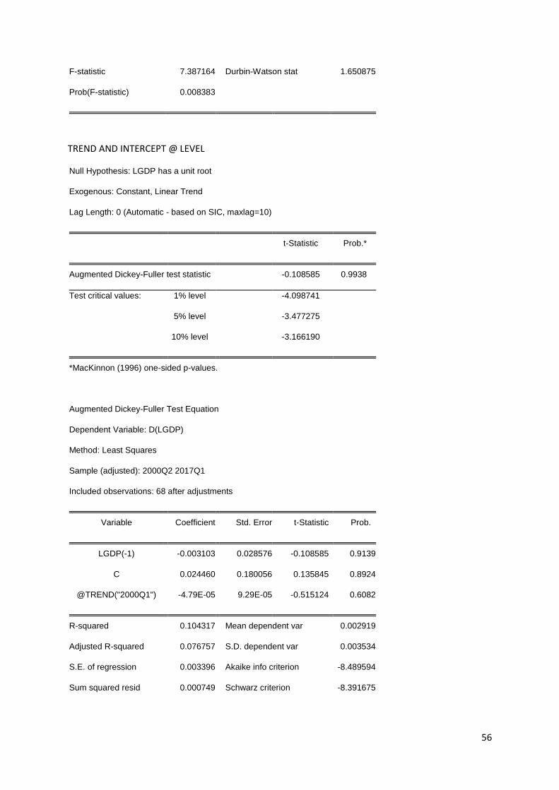
56
F-statistic 7.387164 Durbin-Watson stat 1.650875
Prob(F-statistic) 0.008383
TREND AND INTERCEPT @ LEVEL
Null Hypothesis: LGDP has a unit root
Exogenous: Constant, Linear Trend
Lag Length: 0 (Automatic - based on SIC, maxlag=10)
t-Statistic Prob.*
Augmented Dickey-Fuller test statistic -0.108585 0.9938
Test critical values: 1% level -4.098741
5% level -3.477275
10% level -3.166190
*MacKinnon (1996) one-sided p-values.
Augmented Dickey-Fuller Test Equation
Dependent Variable: D(LGDP)
Method: Least Squares
Sample (adjusted): 2000Q2 2017Q1
Included observations: 68 after adjustments
Variable Coefficient Std. Error t-Statistic Prob.
LGDP(-1) -0.003103 0.028576 -0.108585 0.9139
C 0.024460 0.180056 0.135845 0.8924
@TREND("2000Q1") -4.79E-05 9.29E-05 -0.515124 0.6082
R-squared 0.104317 Mean dependent var 0.002919
Adjusted R-squared 0.076757 S.D. dependent var 0.003534
S.E. of regression 0.003396 Akaike info criterion -8.489594
Sum squared resid 0.000749 Schwarz criterion -8.391675

57
Log likelihood 291.6462 Hannan-Quinn criter. -8.450796
F-statistic 3.785145 Durbin-Watson stat 1.681238
Prob(F-statistic) 0.027863
INTERCEPT @ 1ST DIFFFERENCE
Null Hypothesis: D(LGDP) has a unit root
Exogenous: Constant
Lag Length: 0 (Automatic - based on SIC, maxlag=10)
t-Statistic Prob.*
Augmented Dickey-Fuller test statistic -6.258682 0.0000
Test critical values: 1% level -3.531592
5% level -2.905519
10% level -2.590262
*MacKinnon (1996) one-sided p-values.
Augmented Dickey-Fuller Test Equation
Dependent Variable: D(LGDP,2)
Method: Least Squares
Sample (adjusted): 2000Q3 2017Q1
Included observations: 67 after adjustments
Variable Coefficient Std. Error t-Statistic Prob.
D(LGDP(-1)) -0.759781 0.121396 -6.258682 0.0000
C 0.002216 0.000558 3.971704 0.0002
R-squared 0.376027 Mean dependent var -4.28E-05
Adjusted R-squared 0.366427 S.D. dependent var 0.004376
S.E. of regression 0.003483 Akaike info criterion -8.452371
Sum squared resid 0.000789 Schwarz criterion -8.386559

58
Log likelihood 285.1544 Hannan-Quinn criter. -8.426329
F-statistic 39.17111 Durbin-Watson stat 2.092460
Prob(F-statistic) 0.000000
TREND AND INTERCEPT @ 1ST DIFFERENCE
Null Hypothesis: D(LGDP) has a unit root
Exogenous: Constant, Linear Trend
Lag Length: 0 (Automatic - based on SIC, maxlag=10)
t-Statistic Prob.*
Augmented Dickey-Fuller test statistic -6.893463 0.0000
Test critical values: 1% level -4.100935
5% level -3.478305
10% level -3.166788
*MacKinnon (1996) one-sided p-values.
Augmented Dickey-Fuller Test Equation
Dependent Variable: D(LGDP,2)
Method: Least Squares
Sample (adjusted): 2000Q3 2017Q1
Included observations: 67 after adjustments
Variable Coefficient Std. Error t-Statistic Prob.
D(LGDP(-1)) -0.849077 0.123171 -6.893463 0.0000
C 0.004337 0.001043 4.156524 0.0001
@TREND("2000Q1") -5.30E-05 2.23E-05 -2.373823 0.0206
R-squared 0.426520 Mean dependent var -4.28E-05
Adjusted R-squared 0.408599 S.D. dependent var 0.004376
S.E. of regression 0.003365 Akaike info criterion -8.506905
Sum squared resid 0.000725 Schwarz criterion -8.408188

59
Log likelihood 287.9813 Hannan-Quinn criter. -8.467842
F-statistic 23.79968 Durbin-Watson stat 2.054506
Prob(F-statistic) 0.000000
EXCHANGE RATE
INTERCEPT @ LEVEL
Null Hypothesis: EXCH has a unit root
Exogenous: Constant
Lag Length: 0 (Automatic - based on SIC, maxlag=10)
t-Statistic Prob.*
Augmented Dickey-Fuller test statistic -7.282589 0.0000
Test critical values: 1% level -3.530030
5% level -2.904848
10% level -2.589907
*MacKinnon (1996) one-sided p-values.
Augmented Dickey-Fuller Test Equation
Dependent Variable: D(EXCH)
Method: Least Squares
Sample (adjusted): 2000Q2 2017Q1
Included observations: 68 after adjustments
Variable Coefficient Std. Error t-Statistic Prob.
EXCH(-1) -0.887362 0.121847 -7.282589 0.0000
C 0.108060 0.622012 0.173727 0.8626
R-squared 0.445546 Mean dependent var 0.044118
Adjusted R-squared 0.437146 S.D. dependent var 6.836150
S.E. of regression 5.128728 Akaike info criterion 6.136563

60
Sum squared resid 1736.054 Schwarz criterion 6.201843
Log likelihood -206.6431 Hannan-Quinn criter. 6.162429
F-statistic 53.03610 Durbin-Watson stat 1.967446
Prob(F-statistic) 0.000000
TREND & INTERCEPT @ LEVEL
Null Hypothesis: EXCH has a unit root
Exogenous: Constant, Linear Trend
Lag Length: 0 (Automatic - based on SIC, maxlag=10)
t-Statistic Prob.*
Augmented Dickey-Fuller test statistic -7.226035 0.0000
Test critical values: 1% level -4.098741
5% level -3.477275
10% level -3.166190
*MacKinnon (1996) one-sided p-values.
Augmented Dickey-Fuller Test Equation
Dependent Variable: D(EXCH)
Method: Least Squares
Sample (adjusted): 2000Q2 2017Q1
Included observations: 68 after adjustments
Variable Coefficient Std. Error t-Statistic Prob.
EXCH(-1) -0.887227 0.122782 -7.226035 0.0000
C 0.208085 1.267312 0.164194 0.8701
@TREND("2000Q1") -0.002900 0.031930 -0.090809 0.9279
R-squared 0.445617 Mean dependent var 0.044118
Adjusted R-squared 0.428559 S.D. dependent var 6.836150

61
S.E. of regression 5.167701 Akaike info criterion 6.165848
Sum squared resid 1735.834 Schwarz criterion 6.263767
Log likelihood -206.6388 Hannan-Quinn criter. 6.204647
F-statistic 26.12370 Durbin-Watson stat 1.967927
Prob(F-statistic) 0.000000
LEXPORT
INTERCEPT @ LEVEL
Null Hypothesis: LEXP has a unit root
Exogenous: Constant
Lag Length: 4 (Automatic - based on SIC, maxlag=10)
t-Statistic Prob.*
Augmented Dickey-Fuller test statistic -1.486596 0.5340
Test critical values: 1% level -3.536587
5% level -2.907660
10% level -2.591396
*MacKinnon (1996) one-sided p-values.
Augmented Dickey-Fuller Test Equation
Dependent Variable: D(LEXP)
Method: Least Squares
Sample (adjusted): 2001Q2 2017Q1
Included observations: 64 after adjustments
Variable Coefficient Std. Error t-Statistic Prob.
LEXP(-1) -0.080737 0.054310 -1.486596 0.1425
D(LEXP(-1)) -0.135778 0.127367 -1.066034 0.2908
D(LEXP(-2)) -0.207133 0.123700 -1.674478 0.0994
D(LEXP(-3)) -0.180715 0.120940 -1.494253 0.1405
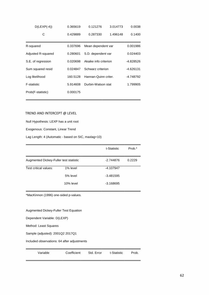
62
D(LEXP(-4)) 0.365619 0.121276 3.014773 0.0038
C 0.429889 0.287330 1.496148 0.1400
R-squared 0.337696 Mean dependent var 0.001986
Adjusted R-squared 0.280601 S.D. dependent var 0.024403
S.E. of regression 0.020698 Akaike info criterion -4.828526
Sum squared resid 0.024847 Schwarz criterion -4.626131
Log likelihood 160.5128 Hannan-Quinn criter. -4.748792
F-statistic 5.914608 Durbin-Watson stat 1.799905
Prob(F-statistic) 0.000175
TREND AND INTERCEPT @ LEVEL
Null Hypothesis: LEXP has a unit root
Exogenous: Constant, Linear Trend
Lag Length: 4 (Automatic - based on SIC, maxlag=10)
t-Statistic Prob.*
Augmented Dickey-Fuller test statistic -2.744876 0.2229
Test critical values: 1% level -4.107947
5% level -3.481595
10% level -3.168695
*MacKinnon (1996) one-sided p-values.
Augmented Dickey-Fuller Test Equation
Dependent Variable: D(LEXP)
Method: Least Squares
Sample (adjusted): 2001Q2 2017Q1
Included observations: 64 after adjustments
Variable Coefficient Std. Error t-Statistic Prob.

63
LEXP(-1) -0.306303 0.111591 -2.744876 0.0081
D(LEXP(-1)) 0.034932 0.143786 0.242944 0.8089
D(LEXP(-2)) -0.066387 0.134301 -0.494314 0.6230
D(LEXP(-3)) -0.088688 0.123469 -0.718301 0.4755
D(LEXP(-4)) 0.428558 0.120253 3.563813 0.0007
C 1.598938 0.581023 2.751936 0.0079
@TREND("2000Q1") 0.000660 0.000288 2.289802 0.0258
R-squared 0.393486 Mean dependent var 0.001986
Adjusted R-squared 0.329643 S.D. dependent var 0.024403
S.E. of regression 0.019980 Akaike info criterion -4.885274
Sum squared resid 0.022754 Schwarz criterion -4.649146
Log likelihood 163.3288 Hannan-Quinn criter. -4.792251
F-statistic 6.163293 Durbin-Watson stat 1.833775
Prob(F-statistic) 0.000050
INTERCEPT @ 1ST DIFFERENCE
Null Hypothesis: D(LEXP) has a unit root
Exogenous: Constant
Lag Length: 3 (Automatic - based on SIC, maxlag=10)
t-Statistic Prob.*
Augmented Dickey-Fuller test statistic -3.762010 0.0053
Test critical values: 1% level -3.536587
5% level -2.907660
10% level -2.591396
*MacKinnon (1996) one-sided p-values.
Augmented Dickey-Fuller Test Equation
Dependent Variable: D(LEXP,2)

64
Method: Least Squares
Sample (adjusted): 2001Q2 2017Q1
Included observations: 64 after adjustments
Variable Coefficient Std. Error t-Statistic Prob.
D(LEXP(-1)) -1.296905 0.344737 -3.762010 0.0004
D(LEXP(-1),2) 0.102397 0.271995 0.376467 0.7079
D(LEXP(-2),2) -0.146376 0.194983 -0.750712 0.4558
D(LEXP(-3),2) -0.353404 0.122232 -2.891265 0.0054
C 0.002764 0.002734 1.010810 0.3162
R-squared 0.697301 Mean dependent var -2.63E-05
Adjusted R-squared 0.676779 S.D. dependent var 0.036777
S.E. of regression 0.020909 Akaike info criterion -4.822381
Sum squared resid 0.025794 Schwarz criterion -4.653718
Log likelihood 159.3162 Hannan-Quinn criter. -4.755936
F-statistic 33.97827 Durbin-Watson stat 1.781889
Prob(F-statistic) 0.000000
TREND & INTERCEPT @ 1ST DIFFERENCE
Null Hypothesis: D(LEXP) has a unit root
Exogenous: Constant, Linear Trend
Lag Length: 3 (Automatic - based on SIC, maxlag=10)
t-Statistic Prob.*
Augmented Dickey-Fuller test statistic -3.740993 0.0266
Test critical values: 1% level -4.107947
5% level -3.481595
10% level -3.168695
*MacKinnon (1996) one-sided p-values.

65
Augmented Dickey-Fuller Test Equation
Dependent Variable: D(LEXP,2)
Method: Least Squares
Sample (adjusted): 2001Q2 2017Q1
Included observations: 64 after adjustments
Variable Coefficient Std. Error t-Statistic Prob.
D(LEXP(-1)) -1.301467 0.347893 -3.740993 0.0004
D(LEXP(-1),2) 0.106573 0.274598 0.388106 0.6994
D(LEXP(-2),2) -0.143621 0.196800 -0.729779 0.4685
D(LEXP(-3),2) -0.351727 0.123362 -2.851184 0.0060
C 0.004177 0.005933 0.703980 0.4843
@TREND("2000Q1") -3.84E-05 0.000143 -0.268975 0.7889
R-squared 0.697678 Mean dependent var -2.63E-05
Adjusted R-squared 0.671616 S.D. dependent var 0.036777
S.E. of regression 0.021075 Akaike info criterion -4.792378
Sum squared resid 0.025762 Schwarz criterion -4.589982
Log likelihood 159.3561 Hannan-Quinn criter. -4.712644
F-statistic 26.76970 Durbin-Watson stat 1.783842
Prob(F-statistic) 0.000000
LIMPORT
INTERCEPT @ LEVEL
Null Hypothesis: LIMP has a unit root
Exogenous: Constant
Lag Length: 0 (Automatic - based on SIC, maxlag=10)
t-Statistic Prob.*
Augmented Dickey-Fuller test statistic -1.594370 0.4800

66
Test critical values: 1% level -3.530030
5% level -2.904848
10% level -2.589907
*MacKinnon (1996) one-sided p-values.
Augmented Dickey-Fuller Test Equation
Dependent Variable: D(LIMP)
Method: Least Squares
Sample (adjusted): 2000Q2 2017Q1
Included observations: 68 after adjustments
Variable Coefficient Std. Error t-Statistic Prob.
LIMP(-1) -0.035910 0.022523 -1.594370 0.1156
C 0.193370 0.117989 1.638884 0.1060
R-squared 0.037087 Mean dependent var 0.005306
Adjusted R-squared 0.022497 S.D. dependent var 0.023473
S.E. of regression 0.023208 Akaike info criterion -4.659678
Sum squared resid 0.035548 Schwarz criterion -4.594399
Log likelihood 160.4291 Hannan-Quinn criter. -4.633812
F-statistic 2.542017 Durbin-Watson stat 2.045722
Prob(F-statistic) 0.115631
TREND & INTERCEPT @ LEVEL
Null Hypothesis: LIMP has a unit root
Exogenous: Constant, Linear Trend
Lag Length: 0 (Automatic - based on SIC, maxlag=10)
t-Statistic Prob.*
Augmented Dickey-Fuller test statistic -1.855959 0.6662

67
Test critical values: 1% level -4.098741
5% level -3.477275
10% level -3.166190
*MacKinnon (1996) one-sided p-values.
Augmented Dickey-Fuller Test Equation
Dependent Variable: D(LIMP)
Method: Least Squares
Sample (adjusted): 2000Q2 2017Q1
Included observations: 68 after adjustments
Variable Coefficient Std. Error t-Statistic Prob.
LIMP(-1) -0.113265 0.061027 -1.855959 0.0680
C 0.580229 0.307193 1.888809 0.0634
@TREND("2000Q1") 0.000529 0.000389 1.362445 0.1778
R-squared 0.063822 Mean dependent var 0.005306
Adjusted R-squared 0.035017 S.D. dependent var 0.023473
S.E. of regression 0.023059 Akaike info criterion -4.658424
Sum squared resid 0.034561 Schwarz criterion -4.560505
Log likelihood 161.3864 Hannan-Quinn criter. -4.619625
F-statistic 2.215627 Durbin-Watson stat 1.947935
Prob(F-statistic) 0.117259
INTERCEPT @ 1ST DIFFERENCE
Null Hypothesis: D(LIMP) has a unit root
Exogenous: Constant
Lag Length: 3 (Automatic - based on SIC, maxlag=10)
t-Statistic Prob.*

68
Augmented Dickey-Fuller test statistic -3.034913 0.0370
Test critical values: 1% level -3.536587
5% level -2.907660
10% level -2.591396
*MacKinnon (1996) one-sided p-values.
Augmented Dickey-Fuller Test Equation
Dependent Variable: D(LIMP,2)
Method: Least Squares
Sample (adjusted): 2001Q2 2017Q1
Included observations: 64 after adjustments
Variable Coefficient Std. Error t-Statistic Prob.
D(LIMP(-1)) -0.829748 0.273401 -3.034913 0.0036
D(LIMP(-1),2) -0.178351 0.222973 -0.799880 0.4270
D(LIMP(-2),2) -0.296238 0.168345 -1.759708 0.0836
D(LIMP(-3),2) -0.394169 0.116635 -3.379498 0.0013
C 0.004569 0.003050 1.498220 0.1394
R-squared 0.622757 Mean dependent var 0.000408
Adjusted R-squared 0.597182 S.D. dependent var 0.033756
S.E. of regression 0.021425 Akaike info criterion -4.773656
Sum squared resid 0.027082 Schwarz criterion -4.604993
Log likelihood 157.7570 Hannan-Quinn criter. -4.707211
F-statistic 24.34951 Durbin-Watson stat 1.841809
Prob(F-statistic) 0.000000
TREND & INTERCEPT @ 1ST DIFFERENCE
Null Hypothesis: D(LIMP) has a unit root
Exogenous: Constant, Linear Trend

69
Lag Length: 3 (Automatic - based on SIC, maxlag=10)
t-Statistic Prob.*
Augmented Dickey-Fuller test statistic -3.244214 0.0852
Test critical values: 1% level -4.107947
5% level -3.481595
10% level -3.168695
*MacKinnon (1996) one-sided p-values.
Augmented Dickey-Fuller Test Equation
Dependent Variable: D(LIMP,2)
Method: Least Squares
Sample (adjusted): 2001Q2 2017Q1
Included observations: 64 after adjustments
Variable Coefficient Std. Error t-Statistic Prob.
D(LIMP(-1)) -0.911331 0.280910 -3.244214 0.0020
D(LIMP(-1),2) -0.118661 0.227764 -0.520984 0.6044
D(LIMP(-2),2) -0.252321 0.171753 -1.469089 0.1472
D(LIMP(-3),2) -0.372774 0.117602 -3.169783 0.0024
C 0.011487 0.006554 1.752696 0.0849
@TREND("2000Q1") -0.000178 0.000149 -1.191331 0.2384
R-squared 0.631768 Mean dependent var 0.000408
Adjusted R-squared 0.600024 S.D. dependent var 0.033756
S.E. of regression 0.021349 Akaike info criterion -4.766581
Sum squared resid 0.026435 Schwarz criterion -4.564186
Log likelihood 158.5306 Hannan-Quinn criter. -4.686847
F-statistic 19.90189 Durbin-Watson stat 1.849053
Prob(F-statistic) 0.000000

70
APPENDIX B: PHILLIPS-PERRON UNIT ROOT TESTS
Null Hypothesis: GDP has a unit root
Exogenous: None
Bandwidth: 5 (Newey-West automatic) using Bartlett kernel
Adj. t-Stat Prob.*
Phillips-Perron test statistic 4.149622 1.0000
Test critical values: 1% level -2.599413
5% level -1.945669
10% level -1.613677
Null Hypothesis: GDP has a unit root
Exogenous: Constant
Bandwidth: 4 (Newey-West automatic) using Bartlett kernel
Adj. t-Stat Prob.*
Phillips-Perron test statistic -1.586992 0.4837
Test critical values: 1% level -3.530030
5% level -2.904848
10% level -2.589907
Null Hypothesis: GDP has a unit root
Exogenous: Constant, Linear Trend
Bandwidth: 4 (Newey-West automatic) using Bartlett kernel
Adj. t-Stat Prob.*
Phillips-Perron test statistic -0.843730 0.9559
Test critical values: 1% level -4.098741
5% level -3.477275
10% level -3.166190

71
Null Hypothesis: D(GDP) has a unit root
Exogenous: None
Bandwidth: 4 (Newey-West automatic) using Bartlett kernel
Adj. t-Stat Prob.*
Phillips-Perron test statistic -4.679389 0.0000
Test critical values: 1% level -2.599934
5% level -1.945745
10% level -1.613633
Null Hypothesis: D(GDP) has a unit root
Exogenous: Constant
Bandwidth: 4 (Newey-West automatic) using Bartlett kernel
Adj. t-Stat Prob.*
Phillips-Perron test statistic -6.695452 0.0000
Test critical values: 1% level -3.531592
5% level -2.905519
10% level -2.590262
Null Hypothesis: D(GDP) has a unit root
Exogenous: Constant, Linear Trend
Bandwidth: 4 (Newey-West automatic) using Bartlett kernel
Adj. t-Stat Prob.*
Phillips-Perron test statistic -6.932077 0.0000
Test critical values: 1% level -4.100935
5% level -3.478305
10% level -3.166788

72
Null Hypothesis: EXCH has a unit root
Exogenous: None
Bandwidth: 2 (Newey-West automatic) using Bartlett kernel
Adj. t-Stat Prob.*
Phillips-Perron test statistic -7.309246 0.0000
Test critical values: 1% level -2.599413
5% level -1.945669
10% level -1.613677
Null Hypothesis: EXCH has a unit root
Exogenous: Constant
Bandwidth: 2 (Newey-West automatic) using Bartlett kernel
Adj. t-Stat Prob.*
Phillips-Perron test statistic -7.255711 0.0000
Test critical values: 1% level -3.530030
5% level -2.904848
10% level -2.589907
Null Hypothesis: EXCH has a unit root
Exogenous: Constant, Linear Trend
Bandwidth: 2 (Newey-West automatic) using Bartlett kernel
Adj. t-Stat Prob.*
Phillips-Perron test statistic -7.196922 0.0000
Test critical values: 1% level -4.098741
5% level -3.477275

73
10% level -3.166190
Null Hypothesis: EXPORT has a unit root
Exogenous: None
Bandwidth: 23 (Newey-West automatic) using Bartlett kernel
Adj. t-Stat Prob.*
Phillips-Perron test statistic 1.545969 0.9690
Test critical values: 1% level -2.599413
5% level -1.945669
10% level -1.613677
Null Hypothesis: EXPORT has a unit root
Exogenous: Constant
Bandwidth: 26 (Newey-West automatic) using Bartlett kernel
Adj. t-Stat Prob.*
Phillips-Perron test statistic -1.888582 0.3357
Test critical values: 1% level -3.530030
5% level -2.904848
10% level -2.589907
Null Hypothesis: EXPORT has a unit root
Exogenous: Constant, Linear Trend
Bandwidth: 5 (Newey-West automatic) using Bartlett kernel
Adj. t-Stat Prob.*
Phillips-Perron test statistic -3.878191 0.0183
Test critical values: 1% level -4.098741

74
5% level -3.477275
10% level -3.166190
Null Hypothesis: D(EXPORT) has a unit root
Exogenous: None
Bandwidth: 57 (Newey-West automatic) using Bartlett kernel
Adj. t-Stat Prob.*
Phillips-Perron test statistic -10.10323 0.0000
Test critical values: 1% level -2.599934
5% level -1.945745
10% level -1.613633
Null Hypothesis: D(EXPORT) has a unit root
Exogenous: Constant
Bandwidth: 34 (Newey-West automatic) using Bartlett kernel
Adj. t-Stat Prob.*
Phillips-Perron test statistic -16.68729 0.0000
Test critical values: 1% level -3.531592
5% level -2.905519
10% level -2.590262
Null Hypothesis: D(EXPORT) has a unit root
Exogenous: Constant, Linear Trend
Bandwidth: 34 (Newey-West automatic) using Bartlett kernel
Adj. t-Stat Prob.*
Phillips-Perron test statistic -18.77689 0.0001

75
Test critical values: 1% level -4.100935
5% level -3.478305
10% level -3.166788
Null Hypothesis: IMPORT has a unit root
Exogenous: None
Bandwidth: 16 (Newey-West automatic) using Bartlett kernel
Adj. t-Stat Prob.*
Phillips-Perron test statistic 1.734336 0.9791
Test critical values: 1% level -2.599413
5% level -1.945669
10% level -1.613677
Null Hypothesis: IMPORT has a unit root
Exogenous: Constant
Bandwidth: 16 (Newey-West automatic) using Bartlett kernel
Adj. t-Stat Prob.*
Phillips-Perron test statistic -1.288125 0.6306
Test critical values: 1% level -3.530030
5% level -2.904848
10% level -2.589907
Null Hypothesis: IMPORT has a unit root
Exogenous: Constant, Linear Trend
Bandwidth: 5 (Newey-West automatic) using Bartlett kernel
Adj. t-Stat Prob.*

76
Phillips-Perron test statistic -2.501771 0.3265
Test critical values: 1% level -4.098741
5% level -3.477275
10% level -3.166190
Null Hypothesis: D(IMPORT) has a unit root
Exogenous: None
Bandwidth: 10 (Newey-West automatic) using Bartlett kernel
Adj. t-Stat Prob.*
Phillips-Perron test statistic -7.981299 0.0000
Test critical values: 1% level -2.599934
5% level -1.945745
10% level -1.613633
Null Hypothesis: D(IMPORT) has a unit root
Exogenous: Constant
Bandwidth: 18 (Newey-West automatic) using Bartlett kernel
Adj. t-Stat Prob.*
Phillips-Perron test statistic -9.190217 0.0000
Test critical values: 1% level -3.531592
5% level -2.905519
10% level -2.590262
Null Hypothesis: D(IMPORT) has a unit root
Exogenous: Constant, Linear Trend
Bandwidth: 20 (Newey-West automatic) using Bartlett kernel
Adj. t-Stat Prob.*

77
Phillips-Perron test statistic -10.19689 0.0000
Test critical values: 1% level -4.100935
5% level -3.478305
10% level -3.166788
APPENDIX C: DF-GLS UNIT ROOT TESTS
INTERCEPT@ LEVEL
Null Hypothesis: LGDP has a unit root
Exogenous: Constant
Lag Length: 2 (Automatic - based on SIC, maxlag=10)
t-Statistic
Elliott-Rothenberg-Stock DF-GLS test statistic 0.337636
Test critical values: 1% level -2.600471
5% level -1.945823
10% level -1.613589
*MacKinnon (1996)
DF-GLS Test Equation on GLS Detrended Residuals
Dependent Variable: D(GLSRESID)
Method: Least Squares
Sample (adjusted): 4 69
Included observations: 66 after adjustments
Variable Coefficient Std. Error t-Statistic Prob.
GLSRESID(-1) 0.001869 0.005534 0.337636 0.7368
D(GLSRESID(-1)) 0.334334 0.117974 2.833953 0.0062

78
D(GLSRESID(-2)) 0.367886 0.118873 3.094787 0.0029
R-squared 0.000289 Mean dependent var 0.002929
Adjusted R-squared -0.031448 S.D. dependent var 0.003586
S.E. of regression 0.003642 Akaike info criterion -8.347930
Sum squared resid 0.000836 Schwarz criterion -8.248401
Log likelihood 278.4817 Hannan-Quinn criter. -8.308601
Durbin-Watson stat 2.163278
TREND & INTERCEPT @LEVEL
Null Hypothesis: LGDP has a unit root
Exogenous: Constant, Linear Trend
Lag Length: 2 (Automatic - based on SIC, maxlag=10)
t-Statistic
Elliott-Rothenberg-Stock DF-GLS test statistic -0.947632
Test critical values: 1% level -3.709200
5% level -3.138800
10% level -2.842000
*Elliott-Rothenberg-Stock (1996, Table 1)
DF-GLS Test Equation on GLS Detrended Residuals
Dependent Variable: D(GLSRESID)
Method: Least Squares
Sample (adjusted): 4 69
Included observations: 66 after adjustments

79
Variable Coefficient Std. Error t-Statistic Prob.
GLSRESID(-1) -0.027059 0.028554 -0.947632 0.3469
D(GLSRESID(-1)) 0.209166 0.123938 1.687666 0.0964
D(GLSRESID(-2)) 0.244416 0.125604 1.945919 0.0561
R-squared 0.111847 Mean dependent var -0.000265
Adjusted R-squared 0.083652 S.D. dependent var 0.003586
S.E. of regression 0.003433 Akaike info criterion -8.466253
Sum squared resid 0.000743 Schwarz criterion -8.366723
Log likelihood 282.3863 Hannan-Quinn criter. -8.426924
Durbin-Watson stat 2.053137
INTERCEPT @1ST DIFFERENCE
Null Hypothesis: D(LGDP) has a unit root
Exogenous: Constant
Lag Length: 1 (Automatic - based on SIC, maxlag=10)
t-Statistic
Elliott-Rothenberg-Stock DF-GLS test statistic -3.761202
Test critical values: 1% level -2.600471
5% level -1.945823
10% level -1.613589
*MacKinnon (1996)
DF-GLS Test Equation on GLS Detrended Residuals
Dependent Variable: D(GLSRESID)

80
Method: Least Squares
Sample (adjusted): 4 69
Included observations: 66 after adjustments
Variable Coefficient Std. Error t-Statistic Prob.
GLSRESID(-1) -0.560395 0.148994 -3.761202 0.0004
D(GLSRESID(-1)) -0.235688 0.122359 -1.926193 0.0585
R-squared 0.400112 Mean dependent var -5.68E-05
Adjusted R-squared 0.390739 S.D. dependent var 0.004408
S.E. of regression 0.003441 Akaike info criterion -8.476482
Sum squared resid 0.000758 Schwarz criterion -8.410129
Log likelihood 281.7239 Hannan-Quinn criter. -8.450263
Durbin-Watson stat 2.051903
TREND & INTERCEPT @1ST DIFFERE
Null Hypothesis: D(LGDP) has a unit root
Exogenous: Constant, Linear Trend
Lag Length: 0 (Automatic - based on SIC, maxlag=10)
t-Statistic
Elliott-Rothenberg-Stock DF-GLS test statistic -6.683496
Test critical values: 1% level -3.705400
5% level -3.135600
10% level -2.839000
*Elliott-Rothenberg-Stock (1996, Table 1)
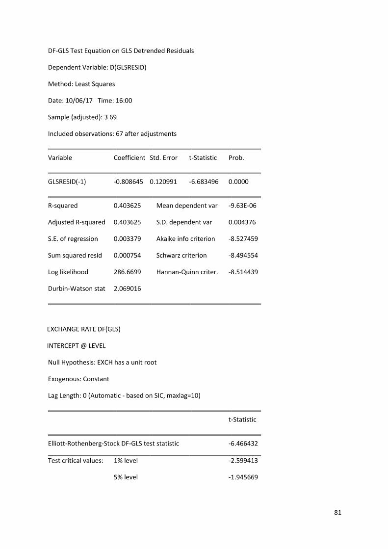
81
DF-GLS Test Equation on GLS Detrended Residuals
Dependent Variable: D(GLSRESID)
Method: Least Squares
Date: 10/06/17 Time: 16:00
Sample (adjusted): 3 69
Included observations: 67 after adjustments
Variable Coefficient Std. Error t-Statistic Prob.
GLSRESID(-1) -0.808645 0.120991 -6.683496 0.0000
R-squared 0.403625 Mean dependent var -9.63E-06
Adjusted R-squared 0.403625 S.D. dependent var 0.004376
S.E. of regression 0.003379 Akaike info criterion -8.527459
Sum squared resid 0.000754 Schwarz criterion -8.494554
Log likelihood 286.6699 Hannan-Quinn criter. -8.514439
Durbin-Watson stat 2.069016
EXCHANGE RATE DF(GLS)
INTERCEPT @ LEVEL
Null Hypothesis: EXCH has a unit root
Exogenous: Constant
Lag Length: 0 (Automatic - based on SIC, maxlag=10)
t-Statistic
Elliott-Rothenberg-Stock DF-GLS test statistic -6.466432
Test critical values: 1% level -2.599413
5% level -1.945669

82
10% level -1.613677
*MacKinnon (1996)
DF-GLS Test Equation on GLS Detrended Residuals
Dependent Variable: D(GLSRESID)
Method: Least Squares
Sample (adjusted): 2 69
Included observations: 68 after adjustments
Variable Coefficient Std. Error t-Statistic Prob.
GLSRESID(-1) -0.768268 0.118809 -6.466432 0.0000
R-squared 0.384249 Mean dependent var 0.044118
Adjusted R-squared 0.384249 S.D. dependent var 6.836150
S.E. of regression 5.364315 Akaike info criterion 6.212011
Sum squared resid 1927.984 Schwarz criterion 6.244651
Log likelihood -210.2084 Hannan-Quinn criter. 6.224944
Durbin-Watson stat 1.984598
TREND & INTERCEPT @ LEVEL
Null Hypothesis: EXCH has a unit root
Exogenous: Constant, Linear Trend
Lag Length: 0 (Automatic - based on SIC, maxlag=10)
t-Statistic
Elliott-Rothenberg-Stock DF-GLS test statistic -7.067557
Test critical values: 1% level -3.701600

83
5% level -3.132400
10% level -2.836000
*Elliott-Rothenberg-Stock (1996, Table 1)
DF-GLS Test Equation on GLS Detrended Residuals
Dependent Variable: D(GLSRESID)
Method: Least Squares
Sample (adjusted): 2 69
Included observations: 68 after adjustments
Variable Coefficient Std. Error t-Statistic Prob.
GLSRESID(-1) -0.853963 0.120829 -7.067557 0.0000
R-squared 0.427107 Mean dependent var 0.004360
Adjusted R-squared 0.427107 S.D. dependent var 6.836150
S.E. of regression 5.174261 Akaike info criterion 6.139867
Sum squared resid 1793.789 Schwarz criterion 6.172506
Log likelihood -207.7555 Hannan-Quinn criter. 6.152800
Durbin-Watson stat 1.963532
INTERCEPT @ 1ST DIFFERE
Null Hypothesis: D(EXCH) has a unit root
Exogenous: Constant
Lag Length: 0 (Automatic - based on SIC, maxlag=10)
t-Statistic
Elliott-Rothenberg-Stock DF-GLS test statistic -10.44462

84
Test critical values: 1% level -2.599934
5% level -1.945745
10% level -1.613633
*MacKinnon (1996)
DF-GLS Test Equation on GLS Detrended Residuals
Dependent Variable: D(GLSRESID)
Method: Least Squares
Sample (adjusted): 3 69
Included observations: 67 after adjustments
Variable Coefficient Std. Error t-Statistic Prob.
GLSRESID(-1) -1.253267 0.119992 -10.44462 0.0000
R-squared 0.622986 Mean dependent var -0.149254
Adjusted R-squared 0.622986 S.D. dependent var 11.40859
S.E. of regression 7.005042 Akaike info criterion 6.745950
Sum squared resid 3238.661 Schwarz criterion 6.778856
Log likelihood -224.9893 Hannan-Quinn criter. 6.758971
Durbin-Watson stat 2.071322
EXPORT @LEVEL DF(GLS)
Null Hypothesis: LEXP has a unit root
Exogenous: Constant
Lag Length: 4 (Automatic - based on SIC, maxlag=10)
t-Statistic

85
Elliott-Rothenberg-Stock DF-GLS test statistic -0.422211
Test critical values: 1% level -2.601596
5% level -1.945987
10% level -1.613496
*MacKinnon (1996)
DF-GLS Test Equation on GLS Detrended Residuals
Dependent Variable: D(GLSRESID)
Method: Least Squares
Sample (adjusted): 6 69
Included observations: 64 after adjustments
Variable Coefficient Std. Error t-Statistic Prob.
GLSRESID(-1) -0.017408 0.041231 -0.422211 0.6744
D(GLSRESID(-1)) -0.150156 0.129311 -1.161200 0.2502
D(GLSRESID(-2)) -0.206918 0.125850 -1.644166 0.1055
D(GLSRESID(-3)) -0.167372 0.122797 -1.362989 0.1781
D(GLSRESID(-4)) 0.388115 0.122689 3.163397 0.0025
R-squared 0.302660 Mean dependent var 0.001986
Adjusted R-squared 0.255383 S.D. dependent var 0.024403
S.E. of regression 0.021057 Akaike info criterion -4.808228
Sum squared resid 0.026161 Schwarz criterion -4.639566
Log likelihood 158.8633 Hannan-Quinn criter. -4.741784
Durbin-Watson stat 1.796151
TREND & INTERCEPT
Null Hypothesis: LEXP has a unit root

86
Exogenous: Constant, Linear Trend
Lag Length: 4 (Automatic - based on SIC, maxlag=10)
t-Statistic
Elliott-Rothenberg-Stock DF-GLS test statistic -2.745379
Test critical values: 1% level -3.716800
5% level -3.145200
10% level -2.848000
*Elliott-Rothenberg-Stock (1996, Table 1)
DF-GLS Test Equation on GLS Detrended Residuals
Dependent Variable: D(GLSRESID)
Method: Least Squares
Sample (adjusted): 6 69
Included observations: 64 after adjustments
Variable Coefficient Std. Error t-Statistic Prob.
GLSRESID(-1) -0.296603 0.108037 -2.745379 0.0080
D(GLSRESID(-1)) 0.027801 0.140785 0.197468 0.8441
D(GLSRESID(-2)) -0.070339 0.131770 -0.533801 0.5955
D(GLSRESID(-3)) -0.090481 0.121485 -0.744789 0.4594
D(GLSRESID(-4)) 0.428100 0.118276 3.619508 0.0006
R-squared 0.390252 Mean dependent var -0.000333
Adjusted R-squared 0.348913 S.D. dependent var 0.024403
S.E. of regression 0.019691 Akaike info criterion -4.942455
Sum squared resid 0.022875 Schwarz criterion -4.773793

87
Log likelihood 163.1586 Hannan-Quinn criter. -4.876010
Durbin-Watson stat 1.829487
INTERCEPT @ 1ST D
Null Hypothesis: D(LEXP) has a unit root
Exogenous: Constant
Lag Length: 3 (Automatic - based on SIC, maxlag=10)
t-Statistic
Elliott-Rothenberg-Stock DF-GLS test statistic -2.657457
Test critical values: 1% level -2.601596
5% level -1.945987
10% level -1.613496
*MacKinnon (1996)
DF-GLS Test Equation on GLS Detrended Residuals
Dependent Variable: D(GLSRESID)
Method: Least Squares
Sample (adjusted): 6 69
Included observations: 64 after adjustments
Variable Coefficient Std. Error t-Statistic Prob.
GLSRESID(-1) -0.689229 0.259357 -2.657457 0.0101
D(GLSRESID(-1)) -0.354089 0.213319 -1.659902 0.1022
D(GLSRESID(-2)) -0.450014 0.160934 -2.796257 0.0069
D(GLSRESID(-3)) -0.504852 0.111465 -4.529250 0.0000

88
R-squared 0.664172 Mean dependent var -2.63E-05
Adjusted R-squared 0.647380 S.D. dependent var 0.036777
S.E. of regression 0.021839 Akaike info criterion -4.749770
Sum squared resid 0.028617 Schwarz criterion -4.614839
Log likelihood 155.9926 Hannan-Quinn criter. -4.696614
Durbin-Watson stat 1.847381
TREND & INTERCEPT @1ST DIFF
Null Hypothesis: D(LEXP) has a unit root
Exogenous: Constant, Linear Trend
Lag Length: 3 (Automatic - based on SIC, maxlag=10)
t-Statistic
Elliott-Rothenberg-Stock DF-GLS test statistic -3.406301
Test critical values: 1% level -3.716800
5% level -3.145200
10% level -2.848000
*Elliott-Rothenberg-Stock (1996, Table 1)
DF-GLS Test Equation on GLS Detrended Residuals
Dependent Variable: D(GLSRESID)
Method: Least Squares
Sample (adjusted): 6 69
Included observations: 64 after adjustments
Variable Coefficient Std. Error t-Statistic Prob.

89
GLSRESID(-1) -1.071284 0.314501 -3.406301 0.0012
D(GLSRESID(-1)) -0.068382 0.250387 -0.273107 0.7857
D(GLSRESID(-2)) -0.260241 0.181967 -1.430159 0.1579
D(GLSRESID(-3)) -0.409785 0.117736 -3.480553 0.0009
R-squared 0.685441 Mean dependent var -4.94E-05
Adjusted R-squared 0.669713 S.D. dependent var 0.036777
S.E. of regression 0.021136 Akaike info criterion -4.815198
Sum squared resid 0.026804 Schwarz criterion -4.680267
Log likelihood 158.0863 Hannan-Quinn criter. -4.762042
Durbin-Watson stat 1.800408
LIMPORT DF GLS
INTERCEPT @ LEVEL
Null Hypothesis: LIMP has a unit root
Exogenous: Constant
Lag Length: 0 (Automatic - based on SIC, maxlag=10)
t-Statistic
Elliott-Rothenberg-Stock DF-GLS test statistic 0.100778
Test critical values: 1% level -2.599413
5% level -1.945669
10% level -1.613677
*MacKinnon (1996)
DF-GLS Test Equation on GLS Detrended Residuals
Dependent Variable: D(GLSRESID)

90
Method: Least Squares
Sample (adjusted): 2 69
Included observations: 68 after adjustments
Variable Coefficient Std. Error t-Statistic Prob.
GLSRESID(-1) 0.001732 0.017183 0.100778 0.9200
R-squared -0.051691 Mean dependent var 0.005306
Adjusted R-squared -0.051691 S.D. dependent var 0.023473
S.E. of regression 0.024072 Akaike info criterion -4.600899
Sum squared resid 0.038825 Schwarz criterion -4.568259
Log likelihood 157.4306 Hannan-Quinn criter. -4.587966
Durbin-Watson stat 1.944839
TREND & INTERCEPT @ LEVEL
Null Hypothesis: LIMP has a unit root
Exogenous: Constant, Linear Trend
Lag Length: 0 (Automatic - based on SIC, maxlag=10)
t-Statistic
Elliott-Rothenberg-Stock DF-GLS test statistic -1.845598
Test critical values: 1% level -3.701600
5% level -3.132400
10% level -2.836000
*Elliott-Rothenberg-Stock (1996, Table 1)
DF-GLS Test Equation on GLS Detrended Residuals
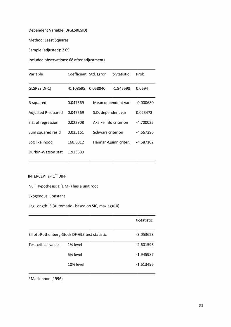
91
Dependent Variable: D(GLSRESID)
Method: Least Squares
Sample (adjusted): 2 69
Included observations: 68 after adjustments
Variable Coefficient Std. Error t-Statistic Prob.
GLSRESID(-1) -0.108595 0.058840 -1.845598 0.0694
R-squared 0.047569 Mean dependent var -0.000680
Adjusted R-squared 0.047569 S.D. dependent var 0.023473
S.E. of regression 0.022908 Akaike info criterion -4.700035
Sum squared resid 0.035161 Schwarz criterion -4.667396
Log likelihood 160.8012 Hannan-Quinn criter. -4.687102
Durbin-Watson stat 1.923680
INTERCEPT @ 1ST DIFF
Null Hypothesis: D(LIMP) has a unit root
Exogenous: Constant
Lag Length: 3 (Automatic - based on SIC, maxlag=10)
t-Statistic
Elliott-Rothenberg-Stock DF-GLS test statistic -3.053658
Test critical values: 1% level -2.601596
5% level -1.945987
10% level -1.613496
*MacKinnon (1996)

92
DF-GLS Test Equation on GLS Detrended Residuals
Dependent Variable: D(GLSRESID)
Method: Least Squares
Sample (adjusted): 6 69
Included observations: 64 after adjustments
Variable Coefficient Std. Error t-Statistic Prob.
GLSRESID(-1) -0.827241 0.270902 -3.053658 0.0034
D(GLSRESID(-1)) -0.180316 0.220953 -0.816080 0.4177
D(GLSRESID(-2)) -0.297727 0.166819 -1.784728 0.0794
D(GLSRESID(-3)) -0.395010 0.115618 -3.416514 0.0011
R-squared 0.622513 Mean dependent var 0.000408
Adjusted R-squared 0.603639 S.D. dependent var 0.033756
S.E. of regression 0.021252 Akaike info criterion -4.804259
Sum squared resid 0.027099 Schwarz criterion -4.669329
Log likelihood 157.7363 Hannan-Quinn criter. -4.751103
Durbin-Watson stat 1.841470
TREND & INTERCEPT @ 1ST DIFF
Null Hypothesis: D(LIMP) has a unit root
Exogenous: Constant, Linear Trend
Lag Length: 3 (Automatic - based on SIC, maxlag=10)
t-Statistic
Elliott-Rothenberg-Stock DF-GLS test statistic -3.225863

93
Test critical values: 1% level -3.716800
5% level -3.145200
10% level -2.848000
*Elliott-Rothenberg-Stock (1996, Table 1)
DF-GLS Test Equation on GLS Detrended Residuals
Dependent Variable: D(GLSRESID)
Method: Least Squares
Sample (adjusted): 6 69
Included observations: 64 after adjustments
Variable Coefficient Std. Error t-Statistic Prob.
GLSRESID(-1) -0.889629 0.275780 -3.225863 0.0020
D(GLSRESID(-1)) -0.134349 0.223877 -0.600101 0.5507
D(GLSRESID(-2)) -0.264928 0.168816 -1.569330 0.1218
D(GLSRESID(-3)) -0.378704 0.115883 -3.267996 0.0018
R-squared 0.628157 Mean dependent var 0.000514
Adjusted R-squared 0.609564 S.D. dependent var 0.033756
S.E. of regression 0.021093 Akaike info criterion -4.819321
Sum squared resid 0.026694 Schwarz criterion -4.684391
Log likelihood 158.2183 Hannan-Quinn criter. -4.766165
Durbin-Watson stat 1.841291
APPENDIX C: ARDL BOUNDS TEST
Sample: 2001Q2 2017Q1
Included observations: 64
Null Hypothesis: No long-run relationships exist

94
Test Statistic Value k F-statistic 5.028621 3
APPENDIX D: ARDL COINTEGRATING AND LONG RUN FORM
ARDL Cointegrating And Long Run Form
Dependent Variable: LGDP
Selected Model: ARDL(1, 0, 2, 5)
Sample: 2000Q1 2017Q4
Included observations: 64
Cointegrating Form
Variable Coefficient Std. Error t-Statistic Prob.
D(EXCH) 0.000002 0.000064 0.027681 0.9780
D(LEXP) 0.084169 0.021041 4.000232 0.0002
D(LEXP(-1)) 0.038482 0.022294 1.726094 0.0903
D(LIMP) -0.008497 0.020818 -0.408162 0.6848
D(LIMP(-1)) -0.023217 0.023491 -0.988345 0.3276
D(LIMP(-2)) -0.000738 0.018623 -0.039621 0.9685
D(LIMP(-3)) 0.057382 0.019903 2.883074 0.0057
D(LIMP(-4)) -0.037806 0.016339 -2.313895 0.0247
CointEq(-1) -0.125246 0.038971 -3.213864 0.0023
Cointeq = LGDP - (0.0000*EXCH -0.3619*LEXP + 0.5788*LIMP + 5.3157 )
Long Run Coefficients
Variable Coefficient Std. Error t-Statistic Prob.
EXCH 0.000014 0.000513 0.027701 0.9780
LEXP -0.361893 0.179090 -2.020737 0.0485
LIMP 0.578821 0.069079 8.379106 0.0000
C 5.315750 0.635277 8.367611 0.0000
Serial correlation
Breusch-Godfrey Serial Correlation LM Test: F-statistic 0.744949 Prob. F(2,50) 0.4800
Obs*R-squared 1.851886 Prob. Chi-Square(2) 0.3962
Test Equation:
Dependent Variable: RESID
Method: ARDL
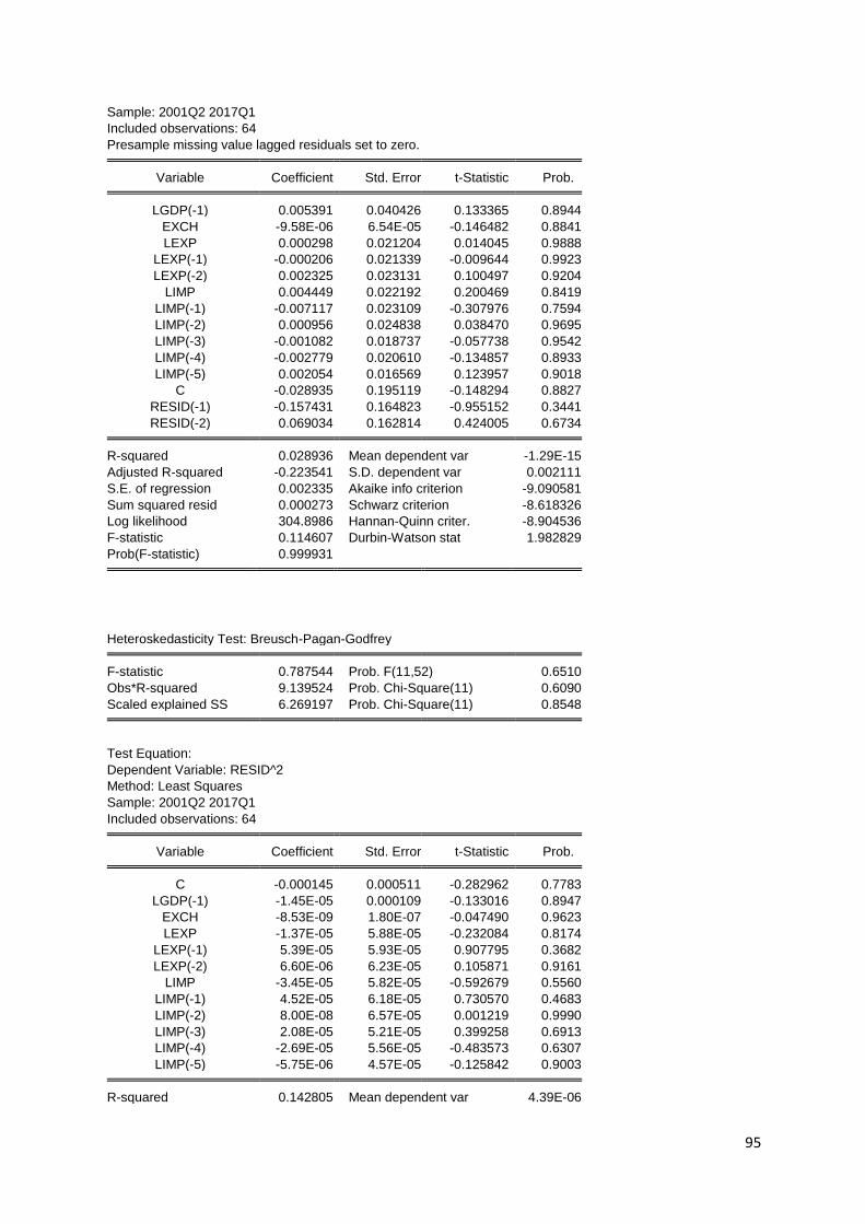
95
Sample: 2001Q2 2017Q1
Included observations: 64
Presample missing value lagged residuals set to zero. Variable Coefficient Std. Error t-Statistic Prob. LGDP(-1) 0.005391 0.040426 0.133365 0.8944
EXCH -9.58E-06 6.54E-05 -0.146482 0.8841
LEXP 0.000298 0.021204 0.014045 0.9888
LEXP(-1) -0.000206 0.021339 -0.009644 0.9923
LEXP(-2) 0.002325 0.023131 0.100497 0.9204
LIMP 0.004449 0.022192 0.200469 0.8419
LIMP(-1) -0.007117 0.023109 -0.307976 0.7594
LIMP(-2) 0.000956 0.024838 0.038470 0.9695
LIMP(-3) -0.001082 0.018737 -0.057738 0.9542
LIMP(-4) -0.002779 0.020610 -0.134857 0.8933
LIMP(-5) 0.002054 0.016569 0.123957 0.9018
C -0.028935 0.195119 -0.148294 0.8827
RESID(-1) -0.157431 0.164823 -0.955152 0.3441
RESID(-2) 0.069034 0.162814 0.424005 0.6734 R-squared 0.028936 Mean dependent var -1.29E-15
Adjusted R-squared -0.223541 S.D. dependent var 0.002111
S.E. of regression 0.002335 Akaike info criterion -9.090581
Sum squared resid 0.000273 Schwarz criterion -8.618326
Log likelihood 304.8986 Hannan-Quinn criter. -8.904536
F-statistic 0.114607 Durbin-Watson stat 1.982829
Prob(F-statistic) 0.999931
Heteroskedasticity Test: Breusch-Pagan-Godfrey F-statistic 0.787544 Prob. F(11,52) 0.6510
Obs*R-squared 9.139524 Prob. Chi-Square(11) 0.6090
Scaled explained SS 6.269197 Prob. Chi-Square(11) 0.8548
Test Equation:
Dependent Variable: RESID^2
Method: Least Squares
Sample: 2001Q2 2017Q1
Included observations: 64 Variable Coefficient Std. Error t-Statistic Prob. C -0.000145 0.000511 -0.282962 0.7783
LGDP(-1) -1.45E-05 0.000109 -0.133016 0.8947
EXCH -8.53E-09 1.80E-07 -0.047490 0.9623
LEXP -1.37E-05 5.88E-05 -0.232084 0.8174
LEXP(-1) 5.39E-05 5.93E-05 0.907795 0.3682
LEXP(-2) 6.60E-06 6.23E-05 0.105871 0.9161
LIMP -3.45E-05 5.82E-05 -0.592679 0.5560
LIMP(-1) 4.52E-05 6.18E-05 0.730570 0.4683
LIMP(-2) 8.00E-08 6.57E-05 0.001219 0.9990
LIMP(-3) 2.08E-05 5.21E-05 0.399258 0.6913
LIMP(-4) -2.69E-05 5.56E-05 -0.483573 0.6307
LIMP(-5) -5.75E-06 4.57E-05 -0.125842 0.9003 R-squared 0.142805 Mean dependent var 4.39E-06

96
Adjusted R-squared -0.038525 S.D. dependent var 6.38E-06
S.E. of regression 6.50E-06 Akaike info criterion -20.88294
Sum squared resid 2.20E-09 Schwarz criterion -20.47815
Log likelihood 680.2540 Hannan-Quinn criter. -20.72347
F-statistic 0.787544 Durbin-Watson stat 1.994210
Prob(F-statistic) 0.651048
Heteroskedasticity Test: Harvey F-statistic 0.877965 Prob. F(11,52) 0.5667
Obs*R-squared 10.02451 Prob. Chi-Square(11) 0.5282
Scaled explained SS 28.99235 Prob. Chi-Square(11) 0.0023
Test Equation:
Dependent Variable: LRESID2
Method: Least Squares
Sample: 2001Q2 2017Q1
Included observations: 64 Variable Coefficient Std. Error t-Statistic Prob. C 134.8509 302.7358 0.445441 0.6579
LGDP(-1) -45.82349 64.54299 -0.709968 0.4809
EXCH 0.117496 0.106456 1.103708 0.2748
LEXP -23.53494 34.84807 -0.675359 0.5024
LEXP(-1) 39.27533 35.15412 1.117232 0.2690
LEXP(-2) -10.29535 36.92357 -0.278829 0.7815
LIMP 8.518754 34.47928 0.247069 0.8058
LIMP(-1) -2.766179 36.60925 -0.075560 0.9401
LIMP(-2) 18.27458 38.90595 0.469712 0.6405
LIMP(-3) 6.634958 30.84378 0.215115 0.8305
LIMP(-4) -35.75827 32.96327 -1.084791 0.2830
LIMP(-5) 27.17692 27.06008 1.004318 0.3199 R-squared 0.156633 Mean dependent var -14.58728
Adjusted R-squared -0.021772 S.D. dependent var 3.807717
S.E. of regression 3.848944 Akaike info criterion 5.700835
Sum squared resid 770.3472 Schwarz criterion 6.105626
Log likelihood -170.4267 Hannan-Quinn criter. 5.860303
F-statistic 0.877965 Durbin-Watson stat 1.981971
Prob(F-statistic) 0.566745
Heteroskedasticity Test: Glejser F-statistic 0.823568 Prob. F(11,52) 0.6172
Obs*R-squared 9.495565 Prob. Chi-Square(11) 0.5762
Scaled explained SS 9.676761 Prob. Chi-Square(11) 0.5597
Test Equation:
Dependent Variable: ARESID
Method: Least Squares

97
Included observations: 64 Variable Coefficient Std. Error t-Statistic Prob. C 0.047972 0.113881 0.421250 0.6753
LGDP(-1) -0.019830 0.024279 -0.816757 0.4178
EXCH 1.59E-05 4.00E-05 0.396669 0.6932
LEXP -0.007818 0.013109 -0.596364 0.5535
LEXP(-1) 0.016589 0.013224 1.254483 0.2153
LEXP(-2) -0.003208 0.013890 -0.230994 0.8182
LIMP -2.88E-05 0.012970 -0.002219 0.9982
LIMP(-1) 0.003016 0.013771 0.219012 0.8275
LIMP(-2) 0.006381 0.014635 0.436016 0.6646
LIMP(-3) 0.004674 0.011603 0.402876 0.6887
LIMP(-4) -0.007067 0.012400 -0.569891 0.5712
LIMP(-5) 0.002816 0.010179 0.276605 0.7832 R-squared 0.148368 Mean dependent var 0.001545
Adjusted R-squared -0.031785 S.D. dependent var 0.001425
S.E. of regression 0.001448 Akaike info criterion -10.07008
Sum squared resid 0.000109 Schwarz criterion -9.665293
Log likelihood 334.2427 Hannan-Quinn criter. -9.910616
F-statistic 0.823568 Durbin-Watson stat 1.906979
Prob(F-statistic) 0.617240
Heteroskedasticity Test: ARCH F-statistic 0.213333 Prob. F(1,61) 0.6458
Obs*R-squared 0.219560 Prob. Chi-Square(1) 0.6394
Test Equation:
Dependent Variable: RESID^2
Method: Least Squares
Sample (adjusted): 2001Q3 2017Q1
Included observations: 63 after adjustments Variable Coefficient Std. Error t-Statistic Prob. C 4.17E-06 9.94E-07 4.201641 0.0001
RESID^2(-1) 0.059138 0.128039 0.461880 0.6458 R-squared 0.003485 Mean dependent var 4.44E-06
Adjusted R-squared -0.012851 S.D. dependent var 6.41E-06
S.E. of regression 6.46E-06 Akaike info criterion -21.03203
Sum squared resid 2.54E-09 Schwarz criterion -20.96399
Log likelihood 664.5089 Hannan-Quinn criter. -21.00527
F-statistic 0.213333 Durbin-Watson stat 1.975048
Prob(F-statistic) 0.645811
APPENDIX E: RAMSEY RESET
Ramsey RESET Test
Equation: UNTITLED
Specification: LGDP LGDP(-1) EXCH LEXP LEXP(-1) LEXP(-2) LIMP LIMP(
-1) LIMP(-2) LIMP(-3) LIMP(-4) LIMP(-5) C

98
Omitted Variables: Squares of fitted values Value df Probability
t-statistic 0.133163 51 0.8946
F-statistic 0.017732 (1, 51) 0.8946 F-test summary:
Sum of Sq. df Mean
Squares
Test SSR 9.76E-08 1 9.76E-08
Restricted SSR 0.000281 52 5.40E-06
Unrestricted SSR 0.000281 51 5.50E-06
Unrestricted Test Equation:
Dependent Variable: LGDP
Method: ARDL
Sample: 2001Q2 2017Q1
Included observations: 64
Maximum dependent lags: 6 (Automatic selection)
Model selection method: Akaike info criterion (AIC)
Dynamic regressors (6 lags, automatic):
Fixed regressors: C Variable Coefficient Std. Error t-Statistic Prob.* LGDP(-1) 0.649772 1.689981 0.384485 0.7022
EXCH 2.93E-06 6.55E-05 0.044807 0.9644
LEXP 0.062026 0.167635 0.370009 0.7129
LEXP(-1) -0.068388 0.171252 -0.399339 0.6913
LEXP(-2) -0.029351 0.072169 -0.406699 0.6859
LIMP -0.005365 0.031546 -0.170064 0.8656
LIMP(-1) 0.057719 0.143628 0.401868 0.6895
LIMP(-2) 0.018076 0.045309 0.398960 0.6916
LIMP(-3) 0.000719 0.018802 0.038238 0.9696
LIMP(-4) -0.042756 0.111654 -0.382936 0.7034
LIMP(-5) 0.028481 0.071947 0.395858 0.6939
C 1.327151 4.970058 0.267029 0.7905
FITTED^2 0.019737 0.148213 0.133163 0.8946 R-squared 0.998677 Mean dependent var 6.420104
Adjusted R-squared 0.998366 S.D. dependent var 0.058040
S.E. of regression 0.002346 Akaike info criterion -9.092816
Sum squared resid 0.000281 Schwarz criterion -8.654293
Log likelihood 303.9701 Hannan-Quinn criter. -8.920060
F-statistic 3208.422 Durbin-Watson stat 2.279092
Prob(F-statistic) 0.000000 *Note: p-values and any subsequent tests do not account for model
selection.