The Effect of State Income Tax Apportionment and Tax ... · The Effect of State Income Tax...

1

JATAVol. 25, Supplement2003pp. 1–25

The Effect of State Income TaxApportionment and Tax Incentives

on New Capital ExpendituresSanjay Gupta and Mary Ann Hofmann

ABSTRACT: This study examines how variations in states’ corporate income tax re-gimes affect new capital investment by business. Using U.S. state-aggregated datafrom 1983 to 1996, we find in pooled and fixed-effects regressions that new capitalexpenditures by corporations in the manufacturing sector are decreasing in the incometax burden on property (measured as the product of the statutory tax rate and theproperty factor weight), and increasing at a decreasing rate in investment-related taxincentives. The effect of the income tax burden on property is more pronounced forstates mandating unitary taxation or the throwback rule. Triangulating our empiricalfindings with prior analytical and simulation studies suggests the following hierarchyfor the relative importance of major attributes of state corporate income tax regimes:the unitary or throwback requirement is most influential on incremental capital invest-ment, followed by apportionment weights and tax rates, and, finally, investment-relatedincentives.

Keywords: state taxation; apportionment formula; tax incentives, unitary business prin-ciple, throwback rule.

JEL Classification: H20; H71.

INTRODUCTION

The purpose of this study is to provide empirical evidence on the effects of variationsin states’ corporate income tax regimes on new capital investment by business. Spe-cifically, the study examines whether states with lower income tax burdens on prop-

erty, measured as a combination of statutory corporate income tax rates and apportionmentformula factor weights, experience a higher level of new capital spending by corporations.In addition, the study examines whether such spending is higher in states with more in-vestment-related tax incentives. Finally, the study examines whether the effects of the stateincome tax burden and tax incentives on corporations’ new capital spending differ between

Sanjay Gupta is a Professor at Arizona State University and Mary Ann Hofmann is anAssociate Professor at Andrews University.

We gratefully acknowledge the comments and suggestions from Sonja Rego (discussant) and participants at the2003 The Journal of the American Taxation Association (JATA) Conference; from Richard Dye (discussant of thepaper at the National Tax Association’s 2001 annual conference); from participants at the 2002 American Ac-counting Association Annual Meeting and workshop participants at Arizona State University, University of Florida,and University of California, Los Angeles; and from Don Goldman, Steve Kaplan, Ed Maydew, Gary McGill,Lillian Mills, Tom Omer, Sue Porter, Doug Shackelford, Nathan Stuart, Rebecca Tsui, Michael Williams, and Sung-Soo Yoon. We thank Robert Gary for excellent research assistance. Research support to Professor Gupta wasprovided by the Dean’s Award for Excellence Summer Grant Program funded by the Dean’s Council of 100, TheEconomic Club of Phoenix, and the Alumni of the W.P. Carey School of Business, Arizona State University.

2 Gupta and Hofmann

The Journal of the American Taxation Association, Supplement 2003

states whose income tax base is determined using unitary taxation or the throwback rule,and states without those rules.

Although there is a growing body of literature aimed at understanding the effects ofsubnational fiscal policy on state-level economic activity, the emphasis in many prior studieshas been placed on employment levels and job creation (e.g., Lightner 1999; Goolsbee andMaydew 2000). In contrast, we focus on investment decisions in the form of incrementalcapital spending by corporations. Our focus is motivated in part by the belief that, eventhough job creation continues to occupy center stage in the political rhetoric surroundingstate tax policy, business location and investment decisions typically are the engines thatdrive employment and income growth. Moreover, the limited prior empirical research thatexamines the role of state corporate income taxes on investment location decisions hasyielded ambiguous and contradictory results.1

We contribute to this literature by going beyond the traditional state corporate incometax regime variables—tax rates and apportionment formula weights—that have been con-sidered in the prior studies. Specifically, we also include in our empirical model investment-related tax incentives and tax base differences in the form of unitary (combined) reportingand the throwback rule. We believe all of these attributes of state tax regimes togetherreflect more completely the true burden of the state corporate income tax on businessinvestment. Further, these attributes are likely correlated with each other, given states’ pro-pensity to use them interchangeably as instruments of fiscal policy; thus, not including themjointly could account for the ambiguous results of prior studies.

Using state-aggregated data from 1983 to 1996, we find that the state corporate incometax burden on property has a significant negative effect on new capital expenditures bymanufacturers, whereas the number of investment-related tax incentives available has asignificant positive, though declining, influence on capital spending. Although these resultsare robust to making comparisons across states or within states over time, the economicmagnitude of these effects is modest, at best. For the average state, a one-percentage-pointdecrease in the income tax burden on property is associated with an estimated $2 to $6million increase in capital spending; an additional incentive is associated with an estimated$0.5 to $2.5 million increase in new capital spending.

In our analysis that takes account of tax base differences between the states, we findthat, after controlling for state fixed effects, the results for income tax burden on propertyand tax incentives hold only in the subsample of states that impose unitary taxation or thethrowback rule. Because these tax regimes typically are considered more burdensome, ourresults suggest that the overall advantages of non-unitary and non-throwback tax systemsmay well offset the small-magnitude effects of any differential tax rates or general invest-ment-related tax incentives.

Our empirical analysis based on state-level panel data spanning a 14-year period cap-tures both cross-sectional and time-series variations in state tax regimes and, as such, theresults shed light on the relative importance of tax rates, apportionment formulae, tax in-centives, and the definition of the tax base on business investment decisions. In so doing,our results potentially can inform state tax policymakers. Triangulating our empirical find-ings with prior analytical and simulation studies suggests the unitary and throwback re-quirements are most influential on the location of capital investment, followed by appor-tionment weights and tax rates. Investment-related incentives have the least impact. It is

1 See Bartik (1994) and Wasylenko (1997) for reviews of this literature.

Apportionment, Incentives, and New Capital Expenditures 3


important to note, however, that while we find statistical significance for the tax policyvariables, the economic significance appears almost negligible. Nevertheless, we believethat this is an informative finding because it shows that the economic impact of changingstate corporate income tax variables is not as large as policymakers might expect. Facedwith continuing cutbacks in federal subsidies and threats of a shrinking tax base arisingfrom interstate competition, electronic commerce, and creative accounting and legal prac-tices, many states have adjusted their corporate income tax rate schedules, changed theirapportionment formulae, or offered different tax incentives to stimulate investment and firmlocation within the state. This study’s results provide a basis for evaluating the inevitabletrade-offs confronted in making these choices and suggest the need for caution.

At a broader level, our study contributes to the ongoing policy debate on tax compe-tition, stimulated in part by highly publicized instances of state and local governmentsvying, through various tax subsidies, to influence plant location decisions. Although thetheoretical literature on tax competition between independent governments suggestsstrongly that such competition is wasteful, recent contributions identify some efficiency-enhancing roles (Wilson 1999). Empirical evidence on whether and the extent to which realeconomic decisions are related to variations in state tax regimes can inform this debate(Hofmann 2002).

The rest of the paper proceeds as follows. The second section briefly reviews theprevious research and develops the hypotheses tested in the study; the third section describesour empirical procedures and data; the fourth section presents the results; and the lastsection offers concluding remarks.

HYPOTHESIS DEVELOPMENTReview of Previous Research

Beginning with the pioneering work of Hall and Jorgenson (1967), researchers havedevoted much attention at the national level to the impact of tax policy on investment. Atthe state level, however, empirical studies of the role of tax policy in economic developmenthave focused attention primarily on aggregate employment or changes in employment. Thestudies that have analyzed the impact of state-level tax differentials on capital investmentand the location of industry have yielded far from conclusive results (Wasylenko 1997).For example, Carlton (1979, 1983) studied the location decisions of new firms, and foundthat a weighted average of state corporate and individual income tax rates was not a sig-nificant factor in those decisions. Papke (1987, 1991) regressed new capital expenditureson three different measures of tax burden and found that the effective tax level measure(manufacturing tax revenue/manufacturing gross profits) and the proportional business bur-den measure (state and local taxes from business/ total state and local tax revenues) wereboth insignificant, but the simulated after-tax return measure (based on industry-specificsimulations of the change in the tax liability given an additional investment in the state)was strongly significant. However, in re-estimating Papke’s (1987) results with 1991 data,Tannenwald (1996) found a much smaller tax effect that was statistically insignificant.2

2 While the after-tax rate of return as a measure of tax burden has some appeal because it can be argued that itcaptures many hidden features of the tax code, there are also some conceptual problems. First, applying lessonsfrom theoretical tax competition models, Knight (2001) demonstrates that jurisdictions (such as states used inthis study) rather than firms or individual plants are the appropriate unit of observation, and that after-tax ratesof return do not vary across jurisdictions and, in any case, these rates are endogenous since they depend uponthe distribution of investment across jurisdictions. Second, calculating a after-tax rate of return at the firm levelrequires capturing tax incentives targeted at individual firms, which are increasingly playing a more dominantrole in state tax policy but which are inherently impossible to capture in any empirical study.

4 Gupta and Hofmann


Bartik (1994) reviewed this literature and concluded that the estimated tax elasticityfor investment in the manufacturing sector appears to range from �0.10 to �0.36. ButWasylenko (1997) contends that these elasticities are not measured with much precision,and it would matter a great deal from a policy perspective on which end of the range theactual elasticities lie. Unfortunately, most of these studies overlook the way that the incomeof a multistate firm is apportioned among the states in which it does business (explainedmore fully in the next section), and the specific effect the property (payroll) factor weighthas on the cost of locating property (labor) in a state.

McClure (1980) demonstrates how formulary apportionment transforms the state cor-porate income tax into separate taxes on sales, payroll, and property. Building on McClure(1980), analytical studies by Gordon and Wilson (1986) and Anand and Sansing (2000)show that variation in income tax rates and apportionment factor weights should affectfirms’ economic decisions relating to the location of jobs and property, but empirical studieshave yielded conflicting evidence.3 For example, Weiner (1996) finds that formula appor-tionment has no independent effect on capital-labor ratios across states in 1990, and onlya modest and marginally significant effect on capital spending when examining changes inapportionment formulae from 1982 to 1990. In studying employment changes from 1994to 1995, Lightner (1999) finds that low income tax rates, rather than factor weights, spuremployment growth. Goolsbee and Maydew (2000), however, find that the apportionmentformula, rather than the tax rate, is more influential—using panel data from 1978 through1994, they estimate that double-weighting the sales factor increases manufacturing em-ployment in the state by 1.1 percent. Employing a different methodological approach con-sisting of an eight-region applied general equilibrium model to simulate the effects ofheavier sales factor weights on economic development and corporate tax revenues,Edmiston (2002) finds that a significant positive impact on economic development existsonly in the very long run and that the short-run effects are negligible.

Inconsistencies thus remain about whether changes in formula apportionment can stim-ulate productive activity and, if so, what is the magnitude of these effects. As noted byKlassen (1999) and Edmiston and Arze (2002), further research is necessary to clarify theseinconsistencies. We believe that incorporating the role of tax incentives and differences inthe definition of the tax base (via unitary reporting or the throwback rule) together withformula apportionment can prove beneficial, and we develop those arguments below.

The Apportionment FormulaA key structural feature of the state corporate income tax in the U.S. is the apportion-

ment formula used to subdivide multistate firms’ income among jurisdictions with whichthey have sufficient contact (nexus). In general, a corporation’s business income is appor-tioned among the states based on what portion of its sales, payroll, and property occur ineach state. The theory is that these factors will fairly reflect the tax attributable to eachstate. Specifically, a multistate firm’s income tax expense, x, in any particular state i iscomputed by the following formula:

3 We should point out that studies examining tax-planning responses rather than real economic effects to state taxregime differences have had more success. For example, in state-aggregated data, Klassen and Shackelford (1998)find that companies likely structured their shipments strategically so as to reduce sales in states that apply ahigh assessment to gross receipts through the apportionment system. Similarly, in firm-level data, Gupta andMills (2002) find that firms’ state effective tax rates first increase and then decrease with the number of statesin which they do business, consistent with their strategic use of tax regime differences, including apportionmentformula, to lower their tax burdens.



s l pi i is L Px � w � w � (w � r ,* * * * *�� i i i i iS L P

where � is the firm’s U.S. (or worldwide) taxable income; ri is the statutory tax rate instate i; si, li, and pi are the firm’s sales, payroll, and property in state i, while S, L, and Pare the firm’s total sales, payroll, and property; and w , and are the factor weightsS L P, w wi i i

in state i for sales, payroll, and property, respectively, that must sum to 1. Thus, the termin the brackets captures the percentage of a firm’s income taxable in state i.

McLure (1980) has demonstrated that, to the extent tax rates vary across jurisdictions,this three-factor apportionment formula effectively transforms the state corporate incometax into separate (excise) taxes on sales, payroll, and property. For example, when a mul-tistate firm invests in new property, the property ratio will increase in that state, which, inturn, will increase the amount of income tax paid to that state by � (pi /P) * * ri, or byPwi

the change in the property ratio times the income tax burden on property. The propertyratio will decrease in all other states (because the denominator is now larger), and lowerthe income taxes paid to those states. Other things being equal, these effects provide thefirm with an incentive to locate property in states with lower property factor weights andtax rates.

These effects also provide states with an incentive to lower the property factor weightin order to attract new business investment.4 Figure 1 illustrates the changes that have takenplace in states’ apportionment formulae during the time span covered by our data. Consis-tent with the states’ incentives, the trend away from equally weighting the factors towarddouble-weighted sales or even 100 percent sales has been increasing since the late 1980s.

The combined, multiplicative effect of the property factor weight and the tax rate leadsto the first hypothesis, stated in alternate form:

H1: Ceteris paribus, new capital expenditures in a state are decreasing in its incometax burden on property.

Investment-Related Tax IncentivesApart from varying apportionment factor weights, states have also competed aggres-

sively with each other by offering a variety of tax incentives. These actions have beenmotivated in part by the fact that changes to statutory rate schedules or the apportionmentformulas have far-reaching impacts on a state’s tax revenues. A tax credit, on the otherhand, can be a more flexible tool for providing economic incentives to businesses—it canbe less permanent than a change in rates or apportionment formula, targeted to a specificsector of the economy, and structured to reward only incremental investments.

While the Tax Reform Act of 1986 did away with the federal investment tax credit, anumber of states have not only preserved their investment tax credit, but have also enactednew or expanded investment-related tax credits, such as enterprise zone credits, new

4 Historically, states have placed equal weights on all three factors such that each factor receives a one-thirdweight. However, states have increasingly begun placing a greater (smaller) weight on the sales (payroll, prop-erty) factor since the U.S. Supreme Court’s decision in Moorman Manufacturing Co. v. Bair, 437 U.S. 267, 98S.Ct. 2340 (1978), which upheld the constitutional validity of Iowa’s single-factor apportionment formula basedsolely on sales. The higher (lower) weight on the sales (property, payroll) factor also serves to export the taxburden to out-of-state firms that typically tend to have less property and payroll within the state. Some studieshave tried to identify the factors associated with states’ decision to switch their apportionment formulae. Omerand Shelley (2002) find that these changes are positively related to the number and timing of changes incompeting states’ apportionment formulae.

6 Gupta and Hofmann


FIGURE 1Trends in Apportionment

0

5

10

15

20

25

30

35

40

83 84 85 86 87 88 89 90 91 92 93 94 95 96

Year

Nu

mb

er o

f S

tate

s

100% Sales Double weighted sales Equally wieighted apportionment formula

facilities credits, corporate headquarters (relocation) credits, etc. The effect of such incen-tives is to lower the tax cost of doing business in the state. Thus, these incentives act assubstitutes for or complements to tax rate changes or apportionment formula changes de-signed to accomplish similar objectives. Consequently, any study of the relationship be-tween state income taxes and economic activity is incomplete, and perhaps misleading (dueto a correlated omitted variable problem), without also considering the effects of tax in-centives.5 Hypothesis 2 follows from the fact that the stated purpose of these tax incentivesis to stimulate business investment:

H2: Ceteris paribus, new capital expenditures in a state are increasing in the invest-ment-related tax incentives available in that state.

Unitary ReportingApart from tax rate and formula apportionment differences, states also differ funda-

mentally in how they define the corporate income tax base, i.e., the computation of a firm’staxable income subject to tax. The primary source of this difference lies in whether thestate applies the unitary business principle. States mandating unitary (combined) reportingdo so by requiring a company to file a combined return with all of its affiliates that forma unitary group. This allows the state to apply its apportionment formula to the combinedincome of a related group of corporations, even though some of the entities in the groupmight not otherwise be taxable in the state. On the other hand, non-unitary (separate re-porting) states require each entity conducting business within the state to file a separatereturn. Non-unitary reporting creates significant tax-planning opportunities for multistateenterprises by allowing them to shift income and profits to low-taxed jurisdictions using

5 Hines (1996) emphasizes this point in his study of the impact of state taxes on the surge in foreign directinvestment in the U.S. during the 1980s.



techniques such as transfer-pricing strategies, passive investment companies, or inter-company loans (Smith 2000).

Recently, Williams et al. (2001) demonstrated analytically and with simulations thattax rate changes cause little or no change in the allocation of property and labor for non-unitary states, but can result in significant changes for unitary states. These conclusions areconsistent with firms in unitary states being less able to use tax-planning techniques tominimize state income taxes, as well as being taxed on a broader base of income (Mooreet al. 1987). Thus, tax burdens tend to be more onerous in unitary states than in non-unitarystates, motivating the following hypothesis:

H3: Ceteris paribus, new capital expenditures in unitary states are decreasing in theincome tax burden on property and by a greater amount than in non-unitary states.

The Throwback RuleAnother feature that affects the apportioned state corporate income tax base is the

throwback rule. The rationale for this rule is to prevent any part of the corporation’s salesfrom being assigned to states where the taxpayer is not taxable and thus escape taxationaltogether. For purposes of the sales factor in the apportionment formula, sales of tangiblepersonal property are sourced to the state to which the goods are shipped or delivered tothe customer (the destination state). If the taxpayer is not taxable in the destination statebecause it lacks sufficient nexus, then those sales are not included in the numerator of thedestination state’s sales factor. States employing the throwback rule, however, reassign(throw back) those sales to the state of origin and include them in the numerator of thatstate’s sales factor. Firms can reduce their overall state effective tax rates by shipping fromnon-throwback states into states where they have no nexus such that those sales are notincluded in the numerator of any state’s sales factor, thus becoming ‘‘orphan’’ or ‘‘nowhere’’sales.

For this reason, the lack of a throwback rule is viewed as a major tax incentive for in-state corporations, and recently some states (e.g., Arizona) have abolished the throwbackrule in order to create incentives for corporations to remain or relocate to the state (Smith2000). Although the throwback rule applies specifically to the sales factor and not theproperty factor per se, which is the main focus of this study, it is possible that companieschoose to locate in non-throwback states so as to be able to engage in the tax planningafforded by the throwback rule. This reasoning motivates the following hypothesis for ourstudy:

H4: New capital expenditures in states employing the throwback rule are decreasing inthe income tax burden on property and by a greater amount than in states notemploying this rule.

EMPIRICAL PROCEDURESModel and Data

To test H1 and H2, we use data aggregated to the state level and estimate pooled andfixed-effects regression models of the following general form:6

Ln(CAPX ) � � � � � BURDEN � � � INCENT � � � VALADD � ε ,it 0 1 it 2 it 3 it�1 it

6 We also estimated this model cross-sectionally for each year and discuss these results (not tabulated) later.

8 Gupta and Hofmann


where CAPX is a measure of the dollar amount of new capital expenditures incurred bythe manufacturing sector in state i in year t, as reported by the U.S. Bureau of Census intheir Annual Survey of Manufactures (1982–1996);7 BURDEN is the product of the propertyfactor weight (PWT) and the average marginal corporate income tax rate (RATE) of statei in year t; INCENT is the number of business tax incentives in state i in year t, as reportedin Site Selection (1982–1995); and VALADD is the value added by the manufacturing sectorin state i in the year t � 1, as reported in the Bureau of Census, Annual Survey of Manu-factures (1982–1996). Apart from VALADD, we include the following additional controlvariables in alternative specifications of the regression model: energy costs (ENRG), definedas the total industrial sector energy price (per million Btu) as reported by the U.S. De-partment of Energy; public expenditures (PUB), defined as the total state and local directgeneral expenditures (less expenditures for welfare) as reported by the U.S. Census Bureau’s(1982–1996) State and Local Government Finances; and census region dummies. Table 1details a complete definition of each variable and the data sources for constructing them,and we discuss below certain measurement issues affecting some of these variables.

The choice of the dependent variable as the dollar amount of new capital expendituresin the manufacturing sector warrants some discussion, especially given the growing im-portance of the nonmanufacturing sectors in our economy. Our choice is motivated byseveral factors. First, the property factor in states’ apportionment formulae includes onlyreal and tangible personal property. Thus, intangibles do not impact the income tax burdenon property that is captured via the apportionment formula. Second, capital expendituresin nonmanufacturing sectors are not readily observable and hence reliable measures are notavailable for each state over time. Both of these reasons probably explain why prior studies(e.g., Carlton 1983; Weiner 1996; Goolsbee and Maydew 2000) are dominated by data fromthe manufacturing sector. Our use of these data allows for better comparability with thesestudies. Finally, concerns about generalizability of our results outside the manufacturingsector are mitigated by the fact that growth in manufacturing correlates highly with thegrowth in state gross domestic product (� � 0.65), an overall measure of states’ economicgrowth that also includes the contributions made by intangibles. For individual states, thiscorrelation ranges between 0.30 and 0.85 during our sample period.8

In constructing BURDEN, we use the top statutory rate as a proxy for the averagemarginal tax rate in each state. While many of the states have progressive tax rate schedules,the top statutory rate is reached at fairly low levels of income. During the time periodcovered by our study, six states allow federal income taxes to be deducted in the compu-tation of state taxable income; for these states, the statutory rate is adjusted for this differ-ence in the tax base.9

Constructing the INCENT variable is complicated. Ideally, we would like to quantifythe relative amount of tax relief available through these incentives across all states over

7 Apart from availability of reliable data, our choice of using state-aggregated data on capital expenditures as theleft-hand side variable, rather than individual firm or plant-level data, is reinforced by Knight’s (2001) recentwork based on tax competition models. He shows that plant-level data, as used in some prior studies (e.g.,Carlton 1983; Papke 1991), violate a key assumption of discrete choice analysis—that of independence of plantlocation choices. Further, we use the natural log of CAPX to correct for the nonlinearity of the relationshipbetween CAPX and the explanatory variables. A Box-Cox subroutine in SAS suggested a log transformation ofY. In addition to creating a tighter model, the log specification allows for the interpretation of the regressioncoefficients as the percentage change in CAPX that results from a one-unit change in the explanatory variables.

8 Only four states (Delaware, Hawaii, Kansas, and Montana) have correlations of less than 0.30 between growthin manufacturing and growth in state gross domestic product. This is not surprising given the large role oftourism and agriculture in these states.

9 The six states are Alabama, Arizona, Louisiana, Missouri, North Dakota, and Iowa. Arizona discontinued thedeductibility of federal income tax in 1990.



TABLE 1Variable Definitions and Data Sources

CAPX � dollar amount (in millions) of new capital expenditures for firms in themanufacturing sector, by state. The measure includes permanent additions and majoralterations to manufacturing establishments, and machinery and equipment subject todepreciation purchased during the year, or leased under capital leases. (See U. S.Census Bureau’s Annual Survey of Manufactures (1982–1996).);

LCAPX � the natural logarithm of CAPX;PWT � the property factor weight used in the state’s apportion formula, expressed as a

percent times 100 (1/4 � 25). (See ACIR’s (1982–1995) Significant Features ofFiscal Federalism and CCH’s (1982–1996) All States Tax Reporter.);

RATE � the top statutory corporate income tax rate, by state, expressed as a percent times100 (5% � 5). (See ACIR’s (1982–1995) Significant Features of Fiscal Federalismand CCH’s (1982–1996) All States Tax Reporter.);

BURDEN � the product of PWT and RATE divided by 100. For a state with a PWT of 25 and aRATE of 5, BURDEN � 1.25;

INCENT � the number of tax incentives for industry. These incentives include: corporateincome tax exemptions; exemptions or moratoriums on land and capitalimprovements; exemptions or moratoriums on equipment and machinery; taxexemptions for manufacturers inventories; sales /use tax exemptions on newequipment; tax exemptions on raw materials used in manufacturing; tax incentivesfor job creation; tax incentives for industrial investment; tax exemptions toencourage R&D; accelerated depreciation for industrial equipment; etc. (See SiteSelection (1982–1995).);

INCENTSQ � the squared value of INCENT;VALADD � dollar amount (in $billions) of value added by the manufacturing sector. This

measure of manufacturing activity is derived by subtracting the cost of materials,supplies, containers, fuel, purchased electricity, and contract work from the value ofshipments (products manufactured plus receipts for services rendered). This figure isadjusted for the net change in finished goods and work-in-process between thebeginning- and end-of-year inventories. Value added is considered to be the bestavailable value measure for comparing the relative economic importance ofmanufacturing among geographic areas. (See U.S. Census Bureau (1982–1996)Annual Survey of Manufactures.);

ENRG � the average total energy price (in nominal dollars per million Btu) for the IndustrialSector. It includes prices for Coal, Natural Gas, Petroleum products, and Electricity.(See U.S. Department of Energy, Energy Information Administration (1995) StateEnergy Price and Expenditure Report 1995.); and

PUB � state and local direct general expenditures (in $millions), less amounts expended forpublic welfare. (See ACIR’s (1982–1995) Significant Features of Fiscal Federalismand U.S. Census Bureau (1982–1996) State and Local Government Finances.)

time. However, these incentives vary widely in the tax base to which they apply, the ratesat which they are allowed, and their qualification criteria, making such quantification vir-tually impossible. Further, state-aggregated data on the cost (in lost revenues) of such taxincentives is not consistently available and, even if available, this measure is likely endog-enous.10 Hence, we define INCENT as the number of tax incentives for industry offered by

10 Even if the data were available, what we would get is the dollar amount of investment-related incentives actuallyused by firms, which would be endogenous to new capital expenditures. Furthermore, that data would still notaccurately reflect the relative amounts of tax relief available across states.

10 Gupta and Hofmann


each state in a given year and obtain the count from Site Selection (1982–1995).11 We usethis count as a rough proxy of tax relief—at the very least, a high count implies a legislativeclimate sympathetic to business.12 We note that our INCENT variable captures only generaltax incentives available to all taxpayers. Targeted tax incentives negotiated with specificfirms are not included in this study as this data is not available; in any event, omitting themshould only bias against finding significant results.

The practice of using tax incentives to compete for new and existing businesses iswidespread (Burstein and Rolnick 1996). Beyond some minimal number of incentives,additional incentives offered by the states are likely to be narrower in scope and offer lessincremental tax relief. Further, two or three narrowly defined incentives may not be betterthan one broad-based incentive. It seems plausible, therefore, to expect a diminishing mar-ginal response to incentives offered by a state. To capture this potential nonlinearity, wealso include INCENTSQ, the square of INCENT, in the model.

VALADD is used to control for size differences across states. In contrast with otherstudies that have used population to control for states’ size (Papke 1987, 1991; Weiner1996), we believe VALADD is more appropriate since it measures the size of the manufac-turing sector in each state’s economy (Klassen and Shackelford 1998).13 To mitigate thepotential endogeneity of VALADD with new capital expenditures, we use a one-year laggedvalue for VALADD.

We begin our sample period with 1983. Data for most of the above variables is availableonly through 1996, so we construct a panel for the 14-year period from 1983–1996. Duringthis time period, there are 44 states that impose a corporate income tax, so there are a totalof 616 (44 � 14) state-year observations.14

Descriptive StatisticsPanel A of Table 2 provides descriptive statistics for the variables included in the model.

The mean (median) dollar amount of new capital expenditures over the 14-year period isalmost $1.9 billion ($1.3 billion). The mean (median) top statutory corporate income taxrate during that period is 7.28 (7.13) percent and ranges from a low of 2.76 percent to a

11 The specific incentives included in the INCENT variable are listed in Table 1. Site Selection is the officialpublication of the International Development Research Council (IDRC) with a reported circulation to over 45,000executives responsible for making location-planning and facility-expansion decisions around the world. SiteSelection’s editorial claims that more than 50 percent of their subscribers are the highest-level managers anddecision makers. The Business Periodicals Index indexes this publication. See http: / /www.siteselection.com formore information.

12 Hines (1996, 1092) also struggles with the quantification of incentives, and concludes that ‘‘it is not possibleto obtain a precise and exogenous measure.’’ In an earlier paper, he also used a count of incentives offered toinvestors but found it to be insignificant in explaining foreign direct investment in the states (Hines 1993).

13 For example, according to 1990 census data, Connecticut and Oklahoma had similar populations, numberingbetween 3.2 and 3.3 million people. However, the more industrialized state of Connecticut had a VALADD of$23.8 billion that year, while the more agrarian Oklahoma had a VALADD of $11.9 billion. One would notexpect the same level of new capital expenditures for the manufacturing sector in Oklahoma as in Connecticut.Thus, population does not adequately control for the size of the manufacturing sector. In any event, we alsoused the gross state product (GSP) as an alternate control for state size. GSP is the state-level counterpart ofgross domestic product (GDP) at the national level. Results with GSP are similar. Finally, in the regressionresults reported later, we also use White’s (1980) procedure to correct for heteroscedasticity created by sizedifferences across states.

14 The six excluded states are Michigan, Nevada, South Dakota, Texas, Washington, and Wyoming. Michigan’sSingle Business Tax is a value-added tax; Texas’ franchise tax was a net-worth tax until 1991; Washington’sbusiness and occupation tax is based on gross receipts; Nevada, South Dakota, and Wyoming impose no businessincome tax. Since some of these states tax businesses in different ways, it did not seem proper to include themin the sample and simply assign an income tax rate of zero. However, for sensitivity purposes, we also estimatedthe regression models including Michigan, Texas, and Washington, as well as including all 50 states, and reportthese results later.



high of 13.80 percent. Half the states during the sample period use a one-third propertyfactor weight, implying an equally weighted formula apportionment. The average numberof incentives offered during the period of the study is 10, and ranges from a low of 3 to ahigh of 14.

Figure 2 shows the trends in the tax variables and new capital expenditures for the 44states in our sample over time. While the mean rate increased slightly—from 7.06 percentin 1983 to a high of 7.6 in 1992, and back down to 7.3 percent in 1996—the decline inthe mean property factor weight has resulted in a slight decline in the mean burden, from2.12 to 1.87 percent. The mean number of incentives increased from 7.7 to 11. However,the mean value for new capital expenditures in the manufacturing sector increased dra-matically from $1.2 billion to $3.4 billion during the same time period.

To better depict the variability in the tax variables over time, Panel B of Table 2categorizes the tax variables (PWT, RATE, BURDEN, and INCENT) into relevant ranges,and reports the number of states whose values fall in each category in each year. The meanof the natural log of capital expenditures is also shown for each category and by year.While the states with the highest property factor weights experienced the lowest new capitalexpenditures, the relation does not hold monotonically across all three categories. Likewise,the mean capital spending of states with the lowest top statutory tax rates is statisticallyindistinguishable from that of the states in the highest rate bracket. In contrast, BURDEN,which is the product of the property factor weight and tax rate, exhibits a significant neg-ative relationship with capital expenditures, supporting H1. With regard to INCENT, stateswith higher numbers of tax incentives seem to have higher capital expenditures, whichsupports H2. Because of the interactive and possibly offsetting relationships among thesetax variables, however, we examine them in a multivariate framework and present the resultsof this analysis next.

Panel C of Table 2 reports pairwise correlation coefficients between the different var-iables used in the regression models. BURDEN is highly correlated with RATE and PWT,which is to be expected since it is the product of those two variables. But the correlationsamong most of the other explanatory variables are less than 0.30, suggesting that the re-gression results should not suffer from harmful multicollinearity. It is interesting to notethat INCENT is negatively correlated with PWT and BURDEN, suggesting that incentivesare likely complements to lower property weights or burdens.

RESULTSResults for the Tax Rate VariablesPooled and Panel Data Regression Results

Table 3 reports the regression results for five models of new capital expenditures, withcoefficient estimates in the first row and related t-statistics (corrected for heteroskedasticityusing White’s (1980) standard errors) in parentheses in the second row. The first columnpresents the results of the basic regression model (Model 1). The coefficient for BURDENis negative, the coefficients on INCENT and INCENTSQ are positive and negative, respec-tively, and all are significant at the .01 level.15 Hypotheses 1 and 2 are supported; newcapital expenditures are declining in the property tax burden, but increasing (at a decreasingrate) for states offering more incentives. Finally, the coefficient for VALADD is positiveand highly significant, as expected.

15 Wald tests confirm the joint significance (at or below the .05 level) of INCENT and INCENTSQ in all modelspresented.

12G

uptaand

Hofm

ann

The

Journalof

theA

merican

TaxationA

ssociation,Supplem

ent2003

TABLE 2Descriptive Statistics

Panel A: Descriptive Statistics for the Variables Based on the Pooled Sample, 1983–1996 (616 state-year observations)

Mean Median Minimum Maximum Std. Dev.

CAPX 1,876 1,271 35 41,034 2,459LCAPX 13.86 14.06 10.45 17.53 1.19PWT 28.96 33 0 50 8.67RATE 7.28 7.13 2.76 13.8 1.94BURDEN 2.09 2.15 0 4.04 0.73INCENT 9.7 10 3 14 2.5VALADDt�1 24,382 15,432 501 178,000 27,292ENRGt�1 6.07 5.88 1.90 15.11 1.74PUBt�1 13,078 7,987 869 127,329 17,034

Panel B: State Tax Characteristics by Year, 1983–1996 (44 observations per year)

Variable Range 1983 1984 1985 1986 1987 1988 1989 1990 1991 1992 1993 1994 1995 1996 TotalMean

LCAPX

PWT �25 3 3 3 3 3 3 3 4 4 4 4 4 4 5 37 14.10225–32 6 6 6 8 9 9 10 10 13 13 17 18 19 24 142 14.588��32 35 35 35 33 32 32 31 30 27 27 23 22 21 15 261 13.522**

RATE �6% 11 11 10 10 9 7 10 9 9 9 9 9 9 9 89 14.1316–8.99% 22 22 23 24 25 28 25 26 24 24 25 25 25 25 171 13.634*�8.99% 11 11 11 10 10 9 9 9 11 11 10 10 10 10 180 14.157

BURDEN �1.75 9 9 9 9 9 8 10 10 12 12 12 12 12 15 112 14.2141.7–2.5 25 24 24 22 22 22 21 20 19 19 23 24 25 24 211 13.888*�2.5 10 11 11 13 13 14 13 14 13 13 9 8 7 5 117 13.483**

INCENT �8 21 20 15 12 11 11 9 8 6 6 6 5 4 4 70 13.2368–11 19 20 24 25 24 23 24 21 22 20 20 21 22 21 218 13.999��11 4 4 5 7 9 10 11 15 16 18 18 18 18 19 152 14.117�

Mean LCAPX 13.42 13.63 13.71 13.61 13.69 13.73 13.89 13.94 13.89 13.96 13.99 14.08 14.18 14.33 13.86

(continued on next page)

Apportionm

ent,Incentives,

andN

ewC

apitalE

xpenditures13

The

Journalof

theA

merican

TaxationA

ssociation,Supplem

ent2003

TABLE 2 (continued)

Panel C: Pairwise Correlation Coefficients Based on the Pooled Sample, 1983–1996 (616 state-year observations)a

LCAPX PWT RATE BURDEN INCENT VALADDt–1 ENRGt–1 PUBt–1

CAPX .694 �.092 .125 .021 .159 .814 �.006 .678LCAPX �.199 .003 �.172 .288 .775 �.055 .612PWT �.104 .682 �.265 �.140 �.035 �.099RATE .611 .028 .208 .222 .212BURDEN �.202 .053 .154 .079INCENT .183 �.133 .237VALADDt–1 .041 .898ENRGt–1 .048

* (�) Mean is significantly less than (more than) the mean of the first category at the .05 level of significance, one-tailed test.** Mean is significantly less than the means of the first two categories at the .05 level of significance, one-tailed test.a Correlations greater than .08 in absolute value are significant at the .05 level of significance (two-tailed test).



FIGURE 2Trends in Tax Variables and Capital Spending

0

5

10

15

20

25

30

35

83 84 85 86 87 88 89 90 91 92 93 94 95 96

Year

Per

cen

t / N

um

ber

of

Ince

nti

ves

/ $10

0,00

0,00

0 o

f N

ew C

apit

al

Exp

end

itu

res

Mean RATE Mean PWT Mean BURDEN Mean INC Mean CAPX

The basic model excludes many factors that are likely to influence capital investmentby firms. To the extent that one or more of these excluded factors is correlated with theexplanatory variables included in the model, the reported coefficient estimates will be bi-ased. Models 2–4 attempt to mitigate this problem in different ways.

Business investment decisions may be affected by regional differences in labor, energy,and transportation costs, as well as by agglomeration economies (Papke 1991). Therefore,in Model 2 we control for geographical variation in these and other macroeconomic factorsby including indicator variables for seven of the eight census regions (the Northeast regionwas omitted). The coefficients for these indicator variables are not presented; instead, thenumber of census regions with significant coefficients is indicated in the table. The coef-ficient estimates and statistical significance of the tax variables under this specification arevirtually identical to Model 1.

As mentioned earlier, previous studies have found variables such as energy prices andpublic expenditures to be statistically significant in models of capital investment (e.g., Papke1987; Weiner 1996). The influence of energy costs on capital expenditures is obvious.Public spending is included to capture the variation across states in the quantity/quality ofpublic goods and services provided (Helms 1985; Mofidi and Stone 1990). For instance,states that provide better highways or better schools might appear more attractive to busi-nesses; thus, public spending has an influence on business location decisions. The corre-lation matrix in Panel B of Table 2 shows that energy prices and public expenditures areboth somewhat correlated with the tax variables included in the basic model; omission ofthe former may result in biased estimates for the latter.

In Model 3, we include variables for energy prices (ENRG) and public expenditures(PUB) as additional controls (instead of the regional dummy variables in Model 2). As withVALADD, we use one-year lagged values for both ENRG and PUB to mitigate against



TABLE 3Regression Results of New Capital Expenditures

Coefficient Estimates from Pooled and Fixed-Effects Regressions of the Following Model for thePeriod 1983–1996 (t-statistics in parentheses; 616 state-year observations):

LCAPX � � � � � BURDEN � � � INCENT � � � INCENTSQ � � � VALADDit 0 1 it 2 it 3 it 4 it�1

� � � ENRG � � � PUB � ε5 it�1 6 it�1 it

Variable(Expected Sign)

Simple Pooled ModelsModel 1 Model 2 Model 3 Model 4

FixedEffectsModel

Model 3

Intercept 11.577(26.21)**

12.315(39.11)**

11.622(31.81)**

12.295(35.35)**

NA

BURDEN (�) �0.315(�9.57)**

�0.293(�6.27)**

�0.275(�7.43)**

�0.313(�6.95)**

�0.097(�2.37)**

INCENT (�) 0.437(4.64)**

0.298(4.14)**

0.391(5.25)**

0.303(4.40)**

0.137(3.43)**

INCENTSQ (�) �0.021(�4.26)**

�0.015(�3.79)**

�0.018(�4.38)**

�0.014(�3.77)**

�0.005(�2.13)*

VALADDt�1 (�) 0.033(17.13)**

0.033(22.84)**

0.050(22.99)**

0.047(23.01)**

0.026(9.56)**

ENRGt�1 (?) �0.013(�0.83)

�0.008(�0.54)

�0.077(�4.65)**

PUBt�1 (?) �0.03(�8.61)**

�0.024(�8.04)**

�0.015(�5.27)**

Number of SignificantCensus Regionsa

NA 5 NA 5 NA

Adj. R2 0.67 0.78 0.70 0.79 0.96

#, * and ** denotes significance at the .10, .05 and .01 levels (one-tailed test where directional predictions weremade), respectively.a Models 2 and 4 include indicator variables for 7 of the 8 Census regions. The Northeast region was omitted.The coefficients for constant terms are not shown.The t-statistics are corrected for heteroskedasticity using White’s (1980) standard errors.

potential endogeneity concerns. In Model 4, we include ENRG and PUB, as well as theregional indicator variables. The results from Models 3 and 4 are reported in the third andfourth columns of Table 3. The addition of these control variables does not appear to affectthe sign or significance of the tax variables, although the magnitude of the tax coefficientsis somewhat reduced. With respect to the control variables themselves, new capital expen-ditures are negatively related to both energy prices and public expenditures.16

Apart from energy costs and public expenditures, there are likely to be a whole hostof state-specific factors that may affect capital spending, including state business climate,

16 While the first result is intuitive, the latter requires further discussion. If the comparative level of public expen-ditures represents the quality or quantity of public goods and services in a state, then one would expect a positiverelationship with new capital expenditures by manufacturers. However, to the extent that public expendituresare funded by taxes, higher per-capita public spending may simply reflect higher tax burdens, and thus discouragebusiness expansion. It is this latter effect that appears to dominate in Models 3 and 4, which is also consistentwith the fairly high positive correlation between PUB and RATE in Panel B of Table 2.



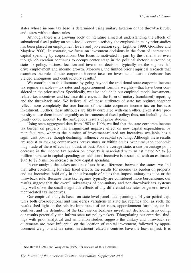
weather, quality of labor force, and endowments of natural resources. To the extent thesestate characteristics influence or are influenced by the state’s fiscal policies, they are po-tentially correlated omitted variables in our model of new capital expenditures. In fact, theplots of the residuals from all of the pooled models show a high degree of correlationamong the 14 observations from each state, suggesting the lack of independence amongthese observations. A fixed-effects specification should control for such influences to theextent they do not vary much over time.

The results of the fixed-effects regression using the 14-year panel estimated for Model3 that includes all control variables (except the regional dummies) are presented in the finalcolumn of Table 3. The likelihood ratio and F-test for the fixed-effects model imply that,although most of the variation in new capital spending across states is explained by statefixed effects, the X-variables do provide significant additional explanatory power.17 As faras the main tax variables are concerned, the coefficient for BURDEN remains negative andsignificant and the coefficient for INCENT is positive and significant. The coefficient forINCENTSQ is negative but insignificant.

Discussion of the ResultsBecause the dependent variable is in log form, the estimated coefficients in the regres-

sion models can be interpreted as the percentage change in new capital expenditures foreach one-unit change in the independent variables. The value of �1 from Model 4 of thepooled regressions in Table 3 is approximately �0.31. This implies that a state whoseBURDEN is one percentage point lower than another state (as it would be, for example, ifthe first state had a top statutory rate of 8 percent and a property weight of one-fourth,while the other state had a top statutory rate of 9 percent and a property weight of one-third), would experience 0.31 percent higher new capital expenditures, ceteris paribus. Atthe mean value for new capital expenditures, this represents an additional $6.2 million innew capital spending in the state with the lower income tax burden on property. In thefixed-effects model, the coefficient for BURDEN is much smaller. Using the �1 estimate of�0.097, a state that lowers its income tax burden on property by one percentage point(as it would, for example, if it had a top statutory rate of 12 percent and it went fromequal-weighting to double-weighting sales) would experience a little over $1.8 million inadditional new capital spending. These cross-state and within-state estimates suggest thatthe income tax burden on property does have a statistically significant, but economicallymodest, influence on new capital investment. To put it in perspective, consider the corre-sponding loss in state corporate income taxes collected. In 1996, the mean BURDEN forthe states in our sample was 1.87 percent. A one-percentage-point drop in BURDEN, to0.87 percent, would reduce corporate income tax revenues (at least those related to propertyand payroll) in the average state by more than one-half. The mean amount of state corporateincome taxes collected by the states in our sample was approximately $615.7 million. Thispotential revenue loss seems out of proportion to the capital investment gained, even if thenew business does broaden the tax base.

Given the inclusion of INCENTSQ in the model, the effect on new capital expendituresof adding one more incentive can be calculated using estimates of (�2 � 2�3 * INCENT).So, comparing a state with five incentives to one with six, and using the coefficients fromthe Model 4 pooled regressions, the state with one more incentive would experience ap-proximately (0.303 � [2 � �0.014 � 6]) � 0.135 percent more in capital spending, or

17 The Chi-square statistic for the likelihood ratio test that the X-variables provide incremental explanatory powerover the state fixed effects is 304.59, which is significant at less than the .001 level.



just over $2.5 million at the mean for new capital expenditures. On the other hand, com-paring a state with 11 incentives to one with 12, the state with 12 incentives would expe-rience approximately �0.033 percent, or about $0.62 million less in new capital spending.Using the smaller coefficient estimates from the fixed-effects regressions, these differenceswould be a 0.077 percent ($1.44 million) increase when going from five to six, and a 0.017percent ($0.32 million) increase when going from 11 to 12 incentives. Using the coefficientsfor INCENT and INCENTSQ from the Model 4 pooled regressions, capital spending in-creases with additional incentives up to a point around 11 incentives, which is approxi-mately the mean and median number of incentives in our data. After that, additional in-centives are associated with decreased spending. Using the estimates from the fixed-effectsModel 3, capital spending increases with the addition of incentives up to 14, which is themaximum of the range of our data. Again, it should be pointed out that the revenue lossfrom these incentives might very well exceed the value of the increased investment.

Sensitivity TestsTo examine the sensitivity of our results to data choices and model specification, we

conduct the following additional tests. First, we re-estimated the regressions includingMichigan, Texas, and Washington, the three states with some type of income-based taxationon businesses (see footnote 14), increasing our sample from 44 to 47 states. Similarly, were-estimate the regressions including all 50 states. In each case (results not shown), thecoefficients for BURDEN are of smaller magnitude and significance, while the coefficientsfor INCENT and INCENTSQ are larger and more strongly significant. The basic conclu-sions, however, are unchanged.

Second, with regard to model specification, we experiment with alternatives to theBURDEN variable. As illustrated in the hypothesis development, a new capital expenditurein a state will result in a change in the corporate income tax owed in that state, all elseheld constant, equal to the change in the property ratio times the product of the propertyfactor weight and the tax rate (BURDEN). Because firms making location decisions willlikely consider both tax rates and apportionment weights as a package, we do not considerBURDEN to be an interaction of two independent variables. Indeed, we have no reason tobelieve that either the rate or the factor weight exerts an independent influence on theproperty location decision. Nevertheless, previous studies have examined the separate ef-fects of the factor weights and the income tax rate. While Goolsbee and Maydew (2000)found that the payroll factor weight was far more influential than the tax rate in determiningstate employment, Lightner’s (1999) study led to the opposite conclusion. Hence, we re-estimate the pooled and fixed-effects models, using RATE and PWT instead of BURDEN(results not shown). In the pooled models, the coefficients for both PWT and RATE arenegative and significant. In the fixed-effects models, the coefficients are negative but, whilePWT is significant, RATE is not, a result similar to Goolsbee and Maydew (2000). Likewise,we re-estimate the models using PWT, RATE, and BURDEN (results not shown). In thiscase, PWT and RATE are both mildly positive, while BURDEN is strongly negative (all aresignificant). The results of the sensitivity analysis seem to suggest that, while both PWTand RATE are influential, it is the product of PWT and RATE (that is, the property BURDEN)that best captures the relationship between capital expenditures and income tax factors,particularly for between-state comparisons.

Third, in addition to the income tax burden on property arising from the apportionmentformula, a firm’s decision to locate property may also be influenced by other taxes, notablyproperty taxes levied on real and personal property by state and local governments. Moststates do not have a state-level property tax on real estate; instead, municipalities levy



property taxes that can vary widely from one municipality to the next within a state. A fewstates do have personal property taxes, but often exempt manufacturing equipment and/orinventories from such taxes. Hence, getting a clean measure for property taxes at the statelevel is difficult. Nevertheless, we re-estimate the models including a variable for propertytaxes (results not shown) based on the midpoint of the ranges of state and local prop-erty tax rates reported in Research Institute of America’s (RIA) (1982–1996) All States TaxHandbook for each state-year. The property tax variable is not statistically significant, andits inclusion does not change the signs or magnitudes of the other variables.18

Finally, the fixed-effects model controls for state-specific characteristics that do notvary over time. It is possible, however, that there are macroeconomic factors unique to thetime periods that do not vary across states. To the extent that these period effects arecorrelated with our independent variables, our results could be biased. We address thisconcern two ways. First, we run 14 annual cross-sectional regressions (results not shown).The coefficient estimates for BURDEN, INCENT, and INCENTSQ follow the hypothesizedpattern in all but two years. There is no detectable time trend in the coefficient estimates.Further, the Fama and MacBeth (1973) t-statistics calculated on the cross-sectional meansof coefficient estimates such that they are not affected by the cross-sectional correlationproblem, as well as the Rosenthal (1991) Z-statistics that are measures of combined prob-ability, indicate that all three variables are statistically significant at or below the 0.05 levelacross the 14-year span.19 Second, we estimate a two-way fixed-effects model, which si-multaneously controls for both state-specific and year-specific fixed effects. This specifi-cation results in reduced magnitude and loss of statistical significance for BURDEN andENRG. (However, in the analyses that include interactions between the tax variables andunitary or throwback dummies, discussed later, BURDEN retains its statistical significanceeven in two-way fixed effects models.)

Results for the Tax Base VariablesData Issues

To analyze the effects of unitary taxation and the throwback rule, we first classify statesas either unitary or non-unitary and throwback or non-throwback. While determiningwhether a state has adopted the throwback rule is straightforward, the unitary/non-unitaryclassification is open to interpretation. There are varying degrees to which states require,allow, or optionally impose the unitary principle in the form of combined reporting.20 Instates where combined reporting is permitted but not mandatory, firms are most likely tofile a combined report when it is to their advantage, while states are most likely to imposecombined reporting when it will result in a higher tax liability. Since we are trying toidentify those states in which imposition of the unitary principle results in a more onerous

18 It was suggested that sales taxes and other forms of state taxation also should be included in the analysis, butmeasures for such variables would suffer from the same shortcomings as the property tax variable, leading to acompounding of ‘‘noise.’’ Most measures of business climate are based heavily on income taxation, and wouldthus overlap our other tax variables.

19 The Fama and MacBeth (1973) t-statistics for BURDEN, INCENT, and INCENTSQ are �5.67, 1.58, �1.36,respectively. We also use two Z-statistics, Z1 and Z2, based on Rosenthal (1991) as measures of the combinedprobability that the coefficient in question could be greater than / less than zero in N different samples if thepopulation mean was zero. Z1 � �t / and Z2 � /�(�), where t is the t-statistic for�� df / (df � 2), ��(N � 1)each yearly regression, df is the degrees of freedom in each regression, N is the number of yearly regressions,� is the standard normal deviate corresponding to the statistical significance of t, and � and �(�) are the meanand standard deviation of the N realizations of �.

20 We thank the discussant for prompting us to carefully think about the classification of states as unitary becauseof these variations.



tax burden, we classify as unitary only those states identified in CCH’s (1982–1996) Mul-tistate Income Tax Guide as requiring combined reporting for all unitary businesses.21

Further, it is possible that states’ choice of tax rates or incentives depends on theirdefinition of the tax base, suggesting potential interactions between the tax rate and taxbase variables. To determine whether the subsamples are different enough that they meritbeing examined separately, we perform the Chow test for a structural break between thetwo groups. The test statistics are significant at less than the 0.001 level (the F-statistic is44.06 for the unitary/non-unitary states and 30.35 for the throwback/non-throwback states),confirming that the relationship among the variables differs across the subsamples. Con-sequently, we analyze each subsample separately and Table 4 reports the results of thisanalysis; footnotes to that table list the states that fall in each group.

Univariate Tests and Regression ResultsPanel A of Table 4 presents descriptive statistics for the new capital expenditures and

the tax variables as well as univariate tests of differences in the means of these variablesfor each of the two subgroups. As predicted in H4, throwback states have significantlylower mean CAPX than their counterpart non-throwback states. We do not see this pattern,however, in the unitary/non-unitary subsamples. Unitary states have a significantly higheraverage tax rate, which translates into a higher average BURDEN than non-unitary states.In contrast, throwback states have lower average tax rates but higher property factor weightsfor an overall lower average BURDEN than non-throwback states. In terms of tax incentives,both unitary and throwback states appear to have a significantly lesser number of incentivesavailable than their counterpart non-unitary and non-throwback states, respectively. Thispattern again suggests that INCENT and BURDEN are complements rather than substitutes.

Panel B of Table 4 reports the pooled and fixed-effects regression results separately forunitary/non-unitary states and throwback/non-throwback states. These results are limitedto Model 3 that includes the control variables VALADD, ENRG, and PUB (although thecoefficient estimates for these variables are not presented in the table). While the pooledregressions show that BURDEN has a significantly negative impact on LCAPX for allgroups, the coefficients imply that this effect is larger for unitary and throwback states thanfor their counterpart non-unitary and non-throwback states, respectively. Although theseresults are consistent with H3 and H4, the panel regressions that include a control for statefixed-effects show more clearly the hypothesized effects of unitary and throwback tax re-gimes. Specifically, whereas BURDEN has a significant negative effect on LCAPX in unitaryand throwback states, its effect is positive and/or insignificant in non-unitary and non-throwback states.

With regard to tax incentives, the pooled regressions show that new capital expendituresare increasing (at a decreasing rate) in INCENT in both unitary and throwback states, butthere is little or no association in non-unitary or non-throwback states. This result is partiallyreinforced by the fixed-effects regressions, except that in the unitary/non-unitary analysisincentives appear to have more of an impact in the non-unitary states. As a final check onwhether the regression results for the unitary/non-unitary and throwback/non-throwbacksub-samples are different, we conduct t-tests of differences in the coefficient estimates.

21 For comparison purposes, we re-estimate the models including in our definition of unitary those states that mayrequire combined reporting when separate reporting does not accurately reflect in-state income. (There is onlyone state that permits firms to choose combined reporting but does not retain the right to impose combinedreporting.) Results are similar, but not as strong. We get the most dramatic results when using the list of unitarystates from Williams et al. (2001), but were unable to confirm the basis by which they classify states as unitary.



TABLE 4Descriptive Statistics and Regression Results for Subsamples of States Classified as Unitary/

Non-Unitary and Throwback/Non-Throwback, 1983–1996

Panel A: Descriptive Statistics and Univariate Tests of Differences in Means of New CapitalExpenditures (CAPX) and the Tax Variablesa

UnitaryStates

Non-UnitaryStates

ThrowbackStates

Non-ThrowbackStates

Number of StatesState-years

13182

31434

26364

18252

Mean CAPXMinimumMaximum

1,606,99934,600

14,093,000

1,988,524*122,500

41,034,300

1,468,44134,600

14,093,000

2,464,211*185,600

41,034,300Mean RATEMinimumMaximum

7.624.00

12.00

7.13�2.76

13.80

6.902.769.82

7.83*4.49

13.80Mean PWTMinimumMaximum

290

33

29�0

50

29.970

50

27.5�0

33Mean BURDENMinimumMaximum

2.1803.17

2.05�04.04

2.07503.168

2.1104.04

Mean INCENTMinimumMaximum

93

14

10*4

14

9.3213

14

10.254

14

Panel B: Coefficient Estimates from Pooled and Fixed-Effects Regressions for SeparateSubsamples of Statesb

Dependent Variable is LCAPX; the constant term and the coefficient estimates for the controlvariables VALADD, ENRG, and PUBX are not shown (t-statistics are in parentheses).

Unitary(UNA)States

Non-UnitaryStates

ThrowbackStates

Non-ThrowbackStates

Number of StatesState-years

13182

31434

26364

18252

Cross-Sectional Pooled Model:BURDEN �0.261

(�2.85)**�0.188

(�6.56)**�0.213

(�4.15)**�0.217

(�5.61)**INCENT 0.610

(4.587)**0.087(1.34)#

0.721(7.42)**

0.009(0.01)

INCENTSQ �0.029(�3.89)**

�0.003(�1.00)

�0.036(�6.77)**

�0.001(�0.33)

Adj. R2 .76 .77 .74 .75Fixed-Effects (Panel) Model:BURDEN �0.160

(�2.34)**�0.051

(�0.98)�0.172

(�3.26)**0.082

(1.31)INCENT 0.110

(1.53)#0.140

(2.80)**0.118

(2.11)*0.011

(0.18)INCENTSQ �0.002

(�0.51)�0.006

(�2.28)*�0.002

(�0.75)�0.0002

(�0.07)Adj. R2 .96 .94 .95 .95

(continued on next page)



TABLE 4 (continued)

a * (�) denotes that mean of the first category is significantly less than (more than) the mean of the second categoryat the .05 level of significance, one-tailed test.

b #, * and ** denotes significance at the .10, .05 and .01 levels (one-tailed test where appropriate), respectively.The t-statistics are corrected for heteroskedasticity using White’s (1980) standard errors.States are classified as unitary /non-unitary and as throwback /non-throwback based on CCH’s (1982–1996) Mul-tistate Corporate Income Tax Guide:

Unitary states (UNA) � Alaska, Arizona, California, Hawaii, Idaho, Illinois, Kansas, Maine, Minnesota, Montana,Nebraska, New Hampshire, North Dakota;

Non-unitary states � Alabama, Arkansas, Colorado, Connecticut, Delaware, Florida, Georgia, Indiana, Iowa,Kentucky, Louisiana, Maryland, Massachusetts, Mississippi, Missouri, New Jersey, NewMexico, New York, North Carolina, Ohio, Oklahoma, Oregon, Pennsylvania, Rhode Is-land, South Carolina, Tennessee, Utah, Vermont, Virginia, West Virginia, Wisconsin;

Throwback states � Alabama, Alaska, Arizona, Arkansas, California, Colorado, Hawaii, Idaho, Illinois, In-diana, Kansas, Maine, Massachusetts, Mississippi, Missouri, Montana, Nebraska, NewHampshire, New Mexico, North Dakota, Oklahoma, Oregon, Utah, Vermont, West Vir-ginia (throw-out rule), Wisconsin; and

Non-throwback states � Connecticut, Delaware, Florida, Georgia, Iowa, Kentucky, Louisiana, Maryland, Min-nesota, New Jersey, New York, North Carolina, Ohio, Pennsylvania, Rhode Island, SouthCarolina, Tennessee, Virginia.

These tests confirm that the differences in the coefficient estimates in the regression mod-els between unitary/non-unitary and throwback/non-throwback states are statisticallysignificant.

Sensitivity TestsAlthough the Chow tests of a structural break support analyzing the unitary/non-unitary

and throwback/non-throwback subsamples separately, these specifications are inefficientbecause of the smaller sample sizes. Hence, we also estimate the regression models for allstates together as in Table 3, but including a dummy variable for unitary (throwback) statesand interacting that dummy with BURDEN, INCENT, and INCENTSQ (the dummy is omit-ted in the fixed-effects specifications). The results (not tabulated) yield similar insights asshown in Panel B of Table 4—the coefficients on the interactions between the unitarydummy and BURDEN, INCENT, and INCENTSQ are significantly negative, positive, andnegative, respectively, indicating that tax factors are more influential to the capital invest-ment decision in unitary states. The use of a throwback dummy and interactions yieldssimilar results as the unitary dummy.

It could also be argued that the interaction between unitary and throwback tax regimesis relevant because unitary states that also impose the throwback rule likely have the mostonerous income tax burden on property, whereas the non-unitary/non-throwback states havethe least onerous. Descriptive statistics are consistent with these expectations—a 2 � 2classification (not reported) shows that new capital expenditures are lowest in states thatare both unitary and throwback and highest in states that are neither unitary nor throwback.However, there is a substantial overlap in the states that apply the two tax rules. Specifically,12 of the 13 (92 percent) unitary states also impose the throwback rule, and 17 of the 18(94 percent) non-throwback states are also non-unitary. Thus, any attempts to include bothunitary and throwback dummies and interactions in a full-sample model are unsuccessful.The high correlation between the two classifications prevents a reliable identification oftheir separate and distinct effects.



CONCLUSIONSOur results, based on state-aggregated data from 1983–1996, consistently suggest that

the state corporate income tax burden on property has a statistically significant negativeeffect on new capital expenditures by corporations in the manufacturing sector, whereas thenumber of available investment-related tax incentives has a significant positive, thoughdeclining, influence on incremental capital spending. In further analysis that takes intoaccount tax-base differences among the states, we find that these effects are more pro-nounced in the subsample of states that impose unitary taxation or the throwback rule.Thus, although our study provides evidence that firms tend to locate property in stateswhere they are subject to lower income tax burdens, our results suggest that, on a relativebasis, the advantages of regimes that are non-unitary or do not employ the throwback rulemay well offset the effects of any differential tax rates, apportionment formula weights, orgeneral investment-related tax incentives. Triangulating our empirical findings with prioranalytical and simulation studies (Papke 1996; Williams et al. 2001) suggests that theunitary and throwback requirements are most influential on the location of capital invest-ment, followed by apportionment weights and tax rates, and investment-related incentiveshave the least impact.

While our results are robust to making comparisons across states or within states overtime, the magnitude of these responses is modest, at best; that is, regardless of statisticalsignificance, the economic significance of our coefficients is almost negligible. It is likely,however, that the magnitude effects are understated—in part because of the fundamentalcharacteristics underlying property investment decisions and also because of certain re-search design limitations. First, property, by nature, is not very mobile; once established, afirm would require large tax incentives to overcome the costs of relocation. In addition,since large capital expenditures often are budgeted for years in advance, the timing ofinvestment decisions is likely influenced by past rather than current tax factors. While weonly lagged the control variables, there may also be a considerable lag in firms’ reactionsto changes in tax policy.

Second, our variable measures are not without noise. Specifically, the incremental cap-ital expenditures variable includes routine replacements and additions, which are generallytied to the location of existing property and dilute the role tax factors may play in suchdecisions. Similarly, a simple count of tax incentives available in a state does not measurethe construct with much precision. Third, because most capital decisions are made at thefirm level, our use of state-level aggregated data potentially biases against finding significantresults.22 Finally, we assumed that tax burdens vary exogenously across jurisdictions. It hasbeen argued, however, that state tax rates are likely endogenous since, through the com-petition for capital, they depend on unobserved state characteristics (Knight 2001). Al-though our fixed-effects models control for such characteristics to the extent they do notvary over time, the use of instrumental variables could further cure any remaining endo-geneity concerns.

Notwithstanding these limitations and even allowing for empirical procedures that mayovercome them, it appears that the magnitude of the relationship between new capitalexpenditures and state income tax factors is unlikely to become economically significant.Yet we believe that this is an important finding because it shows that the economic impact

22 In a recent study using firm-level data from Georgia, which switched from an equally weighted three-factorformula to a double-weighted sales formula, Edmiston and Arze (2002) find the tax elasticities to be higher.Specifically, they estimate that the average firm increased its property in Georgia by 5.05 percent following theswitch.



of changing state corporate income tax variables is not as large as policymakers mightexpect. Therefore, our results suggest that state tax policymakers should think carefullyabout using the corporate income tax code as the means for stimulating economic growth,especially in non-unitary and non-throwback states. Although we did not specifically ex-amine the potential impact on state tax revenues, it seems very possible that any incrementalcapital investment resulting from a lowering of the state corporate income tax burden onproperty might be outweighed by the accompanying loss in tax revenues. Altering theapportionment formula or changing tax rates has broad-based implications for all firmsdoing business within the state. As the number of states employing apportionment formulasmore heavily weighted toward sales increases, these apportionment formulas no longerprovide the same level of incentives to corporations. If, as the literature on tax competitionsuggests, states are altering their apportionment formulas and/or rates to remain competitivewith other states that have already done so, then our results reflect the ‘‘race to the bottom’’characterized in other studies (Goolsbee and Maydew 2000). In the long run, a new equi-librium will be reached where all states are collecting less corporate income tax revenueand potentially providing fewer public goods as a result.

Similarly, investment-related tax incentives may also not play as large a role in aggre-gate economic growth as the political rhetoric might suggest. Since we do not have firm-level data, we cannot speak to the impact that targeted tax incentives have on individualfirm decisions. While such incentives when limited to new businesses can contain revenuelosses, the downside is that policymakers may have to contend with claims of inequity fromexisting businesses. Indeed the incidence of such controversy over tax fairness has reachedheightened levels in recent years (Brunori 1997; Burstein and Rolnick 1996). Clearly, theeconomic benefits to be gained from business growth must be weighed against the costs ofoffering major tax incentives.

REFERENCESAmerican Council on Intergovernmental Relations (ACIR). 1982–1995. Significant Features of Fiscal

Federalism. (Formerly U.S. Advisory Council on Intergovernmental Relations.) Washington,D.C.: ACIR.

Anand, B., and R. Sansing. 2000. The weighting game: Formula apportionment as an instrument ofpublic policy. National Tax Journal 53 (2): 183–199.

Bartik, T. 1994. Jobs, productivity, and local economic development: What implications does eco-nomic research have for the role of government? National Tax Journal 47 (4): 847–861.

Brunori, D. 1997. Principles of tax policy and targeted tax incentives. State Tax Notes (June 9): 111–127.

Burstein, M., and A. Rolnick. 1996. Congress should end the economic war among the states. StateTax Notes (June 24): 125–144.

Carlton, D. 1979. Why new firms locate where they do. In Interregional Movements and RegionalGrowth, edited by W. Wheaton. Washington, D.C.: The Urban Institute.

———. 1983. The location and employment choices of new firms: An econometric model withdiscrete and continuous endogenous variables. Review of Economics and Statistics 65 (3): 440–449.

Commerce Clearing House (CCH). 1982–1996. All States Tax Reporter. Chicago, IL: CCH.———. 1982–1996. Multistate Corporate Income Tax Guide. Chicago, IL: CCH.Edmiston, K. 2002. Strategic apportionment of the state corporate income tax. National Tax Journal

55 (2): 239–262.———, and F. Arze. 2002. Firm-level effects of apportionment formula changes. Working paper,

Georgia State University, Atlanta, GA.



Fama, E., and J. MacBeth. 1973. Risk, return, and equilibrium: Empirical tests. The Journal of Po-litical Economy 81 (3): 607–636.

Goolsbee, A., and E. Maydew. 2000. Coveting thy neighbor’s manufacturing: The dilemma of stateincome apportionment. Journal of Public Economics 75 (1): 125–143.

Gordon, R., and J. Wilson. 1986. An examination of multijurisdictional corporate income taxationunder formula apportionment. Econometrica 54 (6): 1357–1373.

Gupta, S., and L. Mills. 2002. Multistate tax planning: Benefits of multiple jurisdictions. Journal ofAccounting and Economics 33 (1): 117–139.

Hall, R., and D. Jorgenson. 1967. Tax policy and investment behavior. American Economic Review57 (3): 391–414.

Helms, L. 1985. The effect of state and local taxes on economic growth: A time series cross-sectionapproach. The Review of Economics and Statistics 67 (4): 574–582.

Hines, J. 1993. Altered states: Taxes and the location of foreign direct investment in America. WorkingPaper No. 4297. Cambridge, MA: National Bureau of Economic Research.

———. 1996. Altered states: Taxes and the location of foreign direct investment in America. Amer-ican Economic Review 86 (5): 1076–1094.

Hofmann, M. 2002. The state corporate income tax: A synthesis of recent research. Journal of Ac-counting Literature 21: 76–119.

Klassen, K., and D. Shackelford. 1998. State and provincial corporate tax planning: Income shiftingand sales apportionment factor management. Journal of Accounting and Economics 25 (3): 385–406.

———. 1999. Discussion of: The effect of the formulary apportionment system on state-level eco-nomic development and multijurisdictional tax planning. The Journal of the American TaxationAssociation 21 (Supplement): 58–62.

Knight, B. 2001. State capital taxes and the location of investment: Empirical lessons from the taxcompetition models. Working paper, Federal Reserve Board, Washington, D.C.

Lightner, T. 1999. The effect of the formulary apportionment system on state-level economic devel-opment and multijurisdictional tax planning. The Journal of the American Taxation Association21 (Supplement): 42–57.

McLure, C. 1980. The state corporate income tax: Lambs in wolves’ clothing. In The Economics ofTaxation, edited by H. Aaron, and M. Boskin. Washington, D.C.: Brookings Institution.

Mofidi, A., and J. Stone. 1990. Do state and local taxes affect economic growth? The Review ofEconomics and Statistics 72 (4): 686–691.

Moore, M., B. Steece, and C. Swenson. 1987. An analysis of the impact of state income tax ratesand bases on foreign investment. The Accounting Review 62 (4): 671–685.

Omer, T., and M. Shelley. 2002. Competitive, political and economic factors influencing state taxpolicy changes. Working paper, University of Illinois at Urbana–Champaign.

Papke, J. 1996. The convergence of state-local business tax costs: Evidence of de facto collaboration.In Proceedings of the 88th Annual Conference of the National Tax Association, 195–206. Co-lumbus, OH: National Tax Association.

Papke, L. 1987. Subnational taxation and capital mobility: Estimates of tax-price elasticities. NationalTax Journal 40 (2): 191–203.

———. 1991. Interstate business tax differentials and new firm location: Evidence from panel data.Journal of Public Economics 45 (1): 47–68.

RIA. 1982–1996. All States Tax Handbook. New York, NY: Research Institute of America.Rosenthal, R. 1991. Meta-Analytic Procedures for Social Research. Newbury Park, CA: Sage

Publications.Site Selection Magazine. 1982–1985. Norcross, GA: Conway Data, Inc.Smith, J. 2000. Guide to state corporate income tax apportionment—Part II. Journal of State Taxation

19 (2): 26–46.Tannenwald, R. 1996. State business tax climate: How should it be measured and how important is

it? New England Economic Review (Jan/Feb): 23–38.



U.S. Census Bureau. Various years. Annual Survey of Manufactures. Washington, D.C.: GovernmentPrinting Office.

———. Various years. State and Local Government Finances. Washington, D.C.: Government Print-ing Office.

U.S. Department of Energy, Energy Information Administration. 1995. State Energy Price and Ex-penditure Report 1995. Washington, D.C.: Government Printing Office.

Wasylenko, M. 1997. Taxation and economic development: The state of the economic literature. NewEngland Economic Review (March/April): 37–52.

Weiner, J. 1996. Estimates of How the Unitary Tax Affects Business Investment. Paper presented atthe Allied Social Science Meetings, San Francisco, California.

White, H. 1980. A heteroscedasticity-consistent covariance matrix estimator and a direct test forheteroscedasticity. Econometrica 48 (May): 817–838.

Williams, M., C. Swenson, and T. Lease. 2001. Effects of unitary versus non-unitary state incometaxes on interstate resource allocation: Some analytical and simulation results. The Journal ofthe American Taxation Association 23 (1): 39–60.

Wilson, J. 1999. Theories of tax competition. National Tax Journal 55 (2): 269–304.

The Effect of State Income Tax Apportionment and Tax ... · The Effect of State Income Tax...

Documents

Transcript of The Effect of State Income Tax Apportionment and Tax ... · The Effect of State Income Tax...