K.7

The Effect of Monetary Policy on Housing Tenure Choice as an Explanation for the Price Puzzle Dias, Daniel A. and João B. Duarte

International Finance Discussion Papers Board of Governors of the Federal Reserve System

Number 1171 June 2016

Please cite paper as: Dias, Daniel A. and João B. Duarte (2016). The Effect of Monetary Policy on Housing Tenure Choice as an Explanation for the Price Puzzle. International Finance Discussion Papers 1171. http://dx.doi.org/10.17016/IFDP.2016.1171

 Board of Governors of the Federal Reserve System  

International Finance Discussion Papers  

Number 1171    

June 2016    

 The Effect of Monetary Policy on Housing Tenure Choice as an Explanation for the Price Puzzle 

 Daniel A. Dias 

 João B. Duarte 

         

      NOTE: International Finance Discussion Papers are preliminary materials circulated to stimulate discussion and critical comment. References to International Finance Discussion Papers (other than an acknowledgment that the writer has had access to unpublished material) should be cleared with the author or authors. Recent IFDPs are available on the Web at www.federalreserve.gov/pubs/ifdp/. This paper can be downloaded without charge from the Social Science Research Network electronic library at www.ssrn.com. 

The effect of monetary policy on housing tenure choice as an

explanation for the price puzzle∗

Daniel A. Dias† Joao B. Duarte‡

June 23, 2016

Abstract

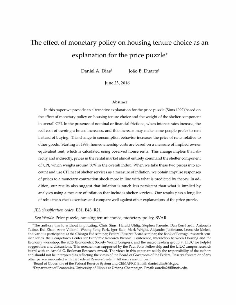
In this paper we provide an alternative explanation for the price puzzle (Sims 1992) based on

the effect of monetary policy on housing tenure choice and the weight of the shelter component

in overall CPI. In the presence of nominal or financial frictions, when interest rates increase, the

real cost of owning a house increases, and this increase may make some people prefer to rent

instead of buying. This change in consumption behavior increases the price of rents relative to

other goods. Starting in 1983, homeownership costs are based on a measure of implied owner

equivalent rent, which is calculated using observed house rents. This change implies that, di-

rectly and indirectly, prices in the rental market almost entirely command the shelter component

of CPI, which weighs around 30% in the overall index. When we take these two pieces into ac-

count and use CPI net of shelter services as a measure of inflation, we obtain impulse responses

of prices to a monetary contraction shock more in line with what is predicted by theory. In ad-

dition, our results also suggest that inflation is much less persistent than what is implied by

analyses using a measure of inflation that includes shelter services. Our results pass a long list

of robustness check exercises and compare well against other explanations of the price puzzle.

JEL classification codes: E31, E43, R21.

Key Words: Price puzzle, housing tenure choice, monetary policy, SVAR.∗The authors thank, without implicating, Chris Sims, Harald Uhlig, Stephen Parente, Dan Bernhardt, Antonella

Tutino, Rui Zhao, Anne Villamil, Woong Yong Park, Igor Ezio, Mark Wright, Alejandro Justiniano, Leonardo Melosi,and various participants at the Chicago Fed seminar, Federal Reserve Board seminar, the Bank of Portugal research sem-inar series, the Georgetown Center for Economic Research Biennial Conference, Interaction between Housing and theEconomy workshop, the 2015 Econometric Society World Congress, and the macro reading group at UIUC for helpfulsuggestions and discussions. This research was supported by the Paul Boltz Fellowship and the UIUC campus researchboard with an Arnold O. Beckman Research Award. The views in this paper are solely the responsibility of the authorsand should not be interpreted as reflecting the views of the Board of Governors of the Federal Reserve System or of anyother person associated with the Federal Reserve System. All errors are our own.†Board of Governors of the Federal Reserve System and CEMAPRE. Email: daniel.dias@frb.gov.‡Department of Economics, University of Illinois at Urbana-Champaign. Email: aurelio2@illinois.edu.

1 Introduction

Using structural vector autoregression (SVAR) analysis, Sims (1992) noted that inflation re-

sponded positively and persistently to a contractionary monetary policy shock. This result is puz-

zling because a central tenet of monetary policy is the ability to control prices by contracting or

expanding monetary supply (vis-a-vis increasing or decreasing interest rates) when prices are above

or below the desired level, respectively. Since this result was first found, and starting with the pa-

per where it was first shown (Sims (1992), several explanations have been proposed. In this paper,

we contribute to this literature by proposing an alternative explanation of the price puzzle based

on the effects of monetary policy on housing tenure choice and the weight of shelter in the overall

consumer price index (CPI).

In Duarte and Dias (2015) we show that, in response to an expansionary monetary policy shock,

house rents decrease while house prices increase. We use the effects of monetary policy on hous-

ing tenure choice decisions together with heterogeneous valuation of homeownership by agents to

explain this result. When interest rates change, the marginal home buyer may change, which may

make house and rent prices change. Because with a higher interest rate the cost of homeowner-

ship may increase, more people may prefer to rent instead of buying. This shift in consumption

behavior makes house prices decrease and rents increase. This mechanism, together with the fact

that shelter, directly and indirectly, accounts for about 30% of the overall CPI, can help explain the

price puzzle. When interest rates increase (a contractionary monetary policy shock), the nominal

price level decreases, but rents will increase if the share of buyers declines and the share of renters

increases. If the increase of rents is sufficiently larger than the decrease of the nominal price level,

then it can be expected that, after a contractionary monetary policy shock, inflation, measured by

CPI, will increase. We test this idea using structural vector autoregression analysis, similar Sims

(1992). Our empirical results strongly support our idea, and when we take into account the effect

of monetary policy on rents and the weight of shelter in CPI, we find that after a contractionary

monetary policy shock, the price puzzle is substantially reduced or even disappears. Our results

are robust to alternative shocks identification strategies, measures of the price level, sample peri-

ods, and identification strategies. Exogenous changes in the construction of CPI allowed us to test

our theory further. In addition, using different measures of inflation, like the personal consumption

expenditure (PCE) and the deflator of gross domestic product (GDP), in which the weight of shel-

ter/housing is lower than in the CPI, permitted us to conduct additional robustness check exercises.

1

As already mentioned, Sims (1992) proposes the first solution to the price puzzle. The author

argues that the puzzle is due to model misspecification and that, when a commodity price index

variable is included in the SVAR model, most of the puzzle disappears. Hanson (2004) shows that

this solution is sensitive to the sample period. In particular, the inclusion of commodity prices

solves the puzzle for sample periods before 1980 but not for posterior sample periods. In line with

the explanation of Sims (1992), several other papers justify the puzzle with model misspecification.

Giordani (2004) argues that the price puzzle is mostly a spurious result due to not including a

measure of the output gap in the empirical model. Once this variable is included in the SVAR model,

the effect of a contractionary monetary policy shock on prices is still positive in the first periods

but then becomes negative. Bernanke, Boivin, and Eliasz (2005) also argue that the SVAR model

used by Sims (1992) was misspecified and suggest the utilization of a factor augmented vector

autoregressive (FAVAR) model to correct for the misspecification. Using the suggested model, the

authors obtain a response of inflation to a contractionary monetary policy shock that is closer to the

expected response. Brissimis and Magginas (2006) also argue that the model used by Sims (1992) is

misspecified and the source of misspecification is the lack of forward-looking variables to account

for expectations at the time of the change of interest rates. To fix this problem, the authors added

the fed funds futures rates and a composite leading indicator of economic activity to the empirical

model. With the new specification, these authors obtain a response of inflation to monetary shocks

that is much more in line with what would be expected.

An alternative line of research that also aims to explain the price puzzle tries to produce theo-

retical models in which prices increase after a contractionary monetary policy shock. One theory

that could deliver such a result is the so-called channel cost of monetary policy (Barth and Ramey

(2001)). To test this hypothesis, Rabanal (2006) estimates a New Keynesian model of the business cy-

cle and tests the conditions under which a cost channel of monetary policy could generate a positive

response of prices to a contractionary monetary policy shock. This author finds that demand side

effects always dominate supply-side effects in prices and, therefore, there is no evidence that the

cost channel of monetary policy can explain the price puzzle. Our results provide some insights on

the type of demand shocks that drive the response of prices. In contrast to Rabanal (2006), Henzel

et al. (2009) estimate a New Keynesian DSGE model for the euro area and argue that, under certain

parameter restrictions, which are not rejected by the data, the channel cost of monetary policy can

explain the price puzzle.

Our contribution combines both types of explanations and adds to them. We also find that the

2

SVAR model in Sims (1992) is misspecified, and suggest a way to improve the specification of the

model. In addition, we provide a theoretical explanation (the effect of monetary policy on housing

tenure choice) for why (some) prices may increase after a contractionary monetary policy shock.

The rest of the paper is organized as follows: in section 2 we discuss some practical issues

regarding the calculation of the CPI; in section 3 we present a simple conceptual framework to

guide our empirical implementation; in section 4 we describe our data and data sources; in section

5 we present our main empirical results; in section 6 we perform several robustness checks; in

section 7 we compare our explanation of the price puzzle to other explanations; and in section 8 we

conclude.

2 Housing in the CPI

In this section we present some information regarding the construction of the CPI and discuss

how some of the methodologies used in the construction of the CPI can help in understanding

the price puzzle. The first aspect about the CPI that we note is that total housing expenses have

a 46% weight in the index. This component has two sub-components, shelter and other housing

related expenses, with the former currently weighing 31% in total CPI and the latter 15%.1 This

information suggests that the overall CPI may be very sensitive to what happens in the housing

component given how large its weight is.

A second aspect to note is that, although the price of most of the sub-components of housing

(e.g., utilities or insurance) are relatively easy to measure, the price of shelter is not. The price of

shelter is easy to measure when someone lives in a house that does not belong to her, but very hard

to measure in the case of someone living in a house that belongs to her. When someone lives in her

own house, there is no established price for the rent that this person would have to pay if she was

renting that same house. Over time, there have been different methods to address this problem,

and these different methods can attenuate or exacerbate the price puzzle.

Before February 1983, the CPI calculated shelter costs differently than what is done today.2 The

cost of housing shelter for homeowners was based on housing prices, mortgage interest rates, prop-

1In this paper, shelter costs only corresponds to rents and the owners’ equivalent rent. The shelter sub-component ofCPI also includes other items which are not relevant to the discussion of the paper. These other items only weigh 1.1% intotal CPI. Hence, total shelter is around 31% and rent plus owners’ equivalent rent is almost 30%.

2For a more detailed discussion about the changes in the CPI methodology, please see Gillingham and Lane (1982)and the BLS document on CPI methodology, “How the CPI measures price change of Owner’s equivalent rent of primaryresidence (OER) and Rent of primary residence (Rent). ”

3

erty taxes, insurance, and maintenance costs. Hence, it included the asset as well as the service

characteristics of housing when estimating the costs of shelter for homeowners. Some problems

with the methodology and with the technical measurement itself were pointed out by the Bureau of

Labor and Statistics (BLS) and the research community. The main concerns raised were the follow-

ing: the difficulty faced by the BLS in correctly estimating the mortgage interest rate cost because of

the new financial contracts involving variable interest rates and specific special arrangements; the

difficulty in estimating housing prices given the small sample and the low frequency with which

houses are traded; the general concern of the BLS that CPI should have a strong credibility and the

possibility that the way housing shelter was being estimated together with its importance in the

CPI could be negatively affecting the credibility of the index; and lastly, the idea that CPI should

be as close as possible as a good measure of consumption expenditure and, hence, homeownership

costs should be computed as closely as possible to a consumption good and not to an asset.

Given the dissatisfaction with how the cost of shelter for homeowners was computed and the

necessity for a more purely consumption-oriented index, the BLS suggested an alternative measure

called owner’s equivalent rent (OER) of primary residence. The idea behind this new measure was

to ask how much rent would the homeowner have to pay if she had to rent her own house. In order

to answer this question, the BLS defined small geographic areas, called segments, within each of

the 87 CPI pricing areas. A segment corresponds to one or more Census blocks. For each segment,

the BLS collects prices from the rental market of houses that are representative of that segment.

This approach allows the BLS to get an implicit rent for owners by comparing houses that have

similar characteristics as the representative ones in the rental market in the same segment. In other

words, the BLS uses hedonic pricing methods to estimate the OER. Hence, the OER is very closely

related to the rental prices observed – the correlation between the level of rental prices and OER is

0.996 while the correlation between the year-on-year growth rates is 0.842. Therefore, the OER can

essentially be seen as a measure of shelter costs faced by homeowners that is based almost solely on

the price of rents from the rental market. The CPI based on this new measure was first introduced

in February 1983, and during a period of six months, until July 1983, the CPI was calculated using

the two measures of shelter costs. This change in methodology allows us to compare the size of the

price puzzle when two alternative measures of shelter costs are used in the construction of the CPI.

In our baseline empirical estimation we consider a sample starting in January 1983 and ending in

December 2006.3

3We truncate the sample at the end of 2006 to avoid the financial crisis period because during this period, there were

4

1985 1990 1995 2000 2005 20100

5

10

15

20

25

30

35

40

Years

Wei

ghti

nC

PI(i

npe

rcen

tage

poin

ts)

ShelterOERRentTotal rent

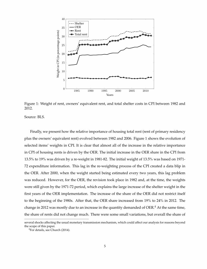
Figure 1: Weight of rent, owners’ equivalent rent, and total shelter costs in CPI between 1982 and2012.

Source: BLS.

Finally, we present how the relative importance of housing total rent (rent of primary residency

plus the owners’ equivalent rent) evolved between 1982 and 2006. Figure 1 shows the evolution of

selected items’ weights in CPI. It is clear that almost all of the increase in the relative importance

in CPI of housing rents is driven by the OER. The initial increase in the OER share in the CPI from

13.5% to 19% was driven by a re-weight in 1981-82. The initial weight of 13.5% was based on 1971-

72 expenditure information. This lag in the re-weighting process of the CPI created a data blip in

the OER. After 2000, when the weight started being estimated every two years, this lag problem

was reduced. However, for the OER, the revision took place in 1982 and, at the time, the weights

were still given by the 1971-72 period, which explains the large increase of the shelter weight in the

first years of the OER implementation. The increase of the share of the OER did not restrict itself

to the beginning of the 1980s. After that, the OER share increased from 19% to 24% in 2012. The

change in 2012 was mostly due to an increase in the quantity demanded of OER.4 At the same time,

the share of rents did not change much. There were some small variations, but overall the share of

several shocks affecting the usual monetary transmission mechanism, which could affect our analysis for reasons beyondthe scope of this paper.

4For details, see Church (2014).

5

rents remained fairly stable. One possible explanation is that the housing sizes for rental units did

not increase as much as the size of the houses that are owned by its occupants. Also, there was a

large increase of homeownership, especially during the 2000-2006 period. This fact seems relevant

in explaining the slight decrease of the weight of rent and the increase of the weight of OER in the

overall CPI in this period.

Before proceeding to the discussion of the conceptual framework, an important remark is in

place. Although all the previous discussion was only about the construction of the CPI, similar

problems are faced by other alternative measures of inflation such as the the PCE and the deflator

of GDP. The problem of estimating the price of shelter is also present in these two indexes, but it

is less important for explaining the price puzzle because the weight of shelter is significantly lower

than in the CPI (15% in the PCE and 13% in the deflator of GDP).

3 The effect of interest rates on the nominal state of the economy and

the CPI

It is well known that the CPI as a measure of monetary inflation has several problems for the

conduct of monetary policy. One of these problems is that the CPI is not able to separate price

changes caused by changes in the nominal state of the economy from price changes caused by

supply and/or demand shocks (relative price changes). The usual way to solve this problem is to

construct measures of core inflation. These can be as simple as removing the more volatile com-

ponents of CPI like energy and unprocessed food, or they can be more elaborate and come out of

econometric models (see Clark (2001) for a survey of core inflation measures). The measurement

issue that we point out in this paper adds to the list of problems with using CPI (or other measures

like the PCE or the deflator of GDP) as a measure of monetary inflation, but it has important dif-

ferences from the other problems previously identified because, according to our idea, the relative

price change is due to changes in interest rates vis-a-vis monetary policy. In order to make our point

clearer, we write the CPI as the product of two components.

CPI(t) = P (t)(αC(t) + (1− α)R(t)) (1)

The first component in equation 1 corresponds to the nominal state of the economy at time t – P(t) –

while the second component corresponds to the real prices of non shelter and shelter consumption

6

– (αC(t) + (1− α)R(t)). In this example we only consider two goods/services, consumption net of

shelter – C(t) – and shelter – R(t) – because we want to focus our discussion on the different behavior

of the two groups of goods/services in response to a monetary shock. In the same equation, α

represents the weight of non-shelter consumption in total consumption.

In Duarte and Dias (2015) we argue that monetary policy affects the choice between housing

tenure (rent vs. own) and therefore the relative prices of the two change when interest rates change.

From our discussion in the previous section, for the purpose of computing the costs of shelter, most

of the information used in these calculations comes from the shelter rental market, which leads

to the shelter component of CPI behaving almost identically to shelter rents. With this in mind,

and with equation 1, we can now discuss when we expect to observe a price puzzle based on our

mechanism.

When the central bank increases interest rates it is normally for the purpose of reducing inflation,

that is, to reduce the growth rate of P(t). If the change in interest rates had no effect on real prices

of shelter and non-shelter goods then it should be expected that, after a contractionary monetary

policy shock, the impulse response function (IRF) of CPI would be negative because the real prices

of both goods would not change. According to our mechanism, after a contractionary monetary

policy shock, not only would P(t), the nominal level of the economy, change, but possibly also R(t),

the price of shelter services. In order for this effect to generate a price puzzle it would be necessary

that the effect of interest rates on R(t), weighed by (1− α), be larger than the effect of interest rates

on P(t):

If∆P (t)

∆i< (1− α)

∆R(t)

∆i=⇒ ∆CPI(t)

∆i> 0 (2)

From equation 2 it is straightforward to see that the smaller the weight of non-shelter goods in

total CPI – α – or the larger the response of shelter prices to interest rates, the more likely it is that

the overall CPI will increase after a contractionary monetary shock.5 This consideration implies that

the ”size” of the price puzzle may be time varying, which is consistent with the findings of Hanson

(2004).

Importantly, and regardless of the overall effect of interest rates changes on total CPI being

positive or negative, based on this discussion, for monetary policy conduct and evaluation, the

shelter component of the CPI (or PCE, or deflator of GDP) should be excluded if the goal is to

5Although our discussion here is informal, in Duarte and Dias (2015) we add an endogenous housing tenure choiceto a standard New Keynesian model, which allows us to have a more formal and precise discussion of this mechanism.

7

measure the nominal state of the economy. In addition, this result also highlights the importance of

using data that are model consistent (or vice-versa).

4 Data

The data that we use in this paper come from multiple sources. The data used in the main

results were collected from the St. Louis Fed Fred economic database. We collected the same four

variables used in Sims (1992) – the federal funds rate (FFR), M1 money stock (M1SL), industrial

production (INDPRO), and CPI index (CPIAUCSL). In addition, we also collected information for

the consumer price index of rent of primary residence (CUSR0000SEHA) and consumer price index

of owners’ equivalent rent of residence (CUSR0000SEHC), which we use to construct the variable

CPI net of shelter. With the exception of the monetary variables (M1SL and FFR), all series were

seasonally adjusted and all variables but the federal funds rate are in log levels. Although most of

our data ranges from 1960 to 2006, our main empirical results concern the period from 1983 to 2006.

We restrict the sample to this period because, as explained in section 2, the CPI suffered a major

revision in 1983 that changed the way shelter costs were estimated. In the same methodological

revision, housing prices were excluded from the CPI.

Because we perform various robustness checks of our main results and also show how our

results compare to previous explanations of the price puzzle, we had to collect several other data. As

alternative inflation measures we use the personal consumption price index (PCE) and the deflator

of GDP. The former is observed at a monthly frequency, while the latter is observed at a quarterly

frequency. Both were obtained from the St. Louis Fed Fred economic database and cover the period

1960 to 2006. As an alternative measure of monetary policy shocks we use the Romer and Romer

(2004) monetary policy shocks measure, which was updated to a more recent period by Coibion et

al. (2012). To replicate the results of Giordani (2004) we used the Federal Reserve Board measure of

capacity utilization, which we obtained from the St. Louis Fed Fred economic database. To replicate

the results of Brissimis and Magginas (2006) we used the composite index of leading indicators

variable that is published by the Conference Board and the expected federal funds rate for the

current month.6 Finally, in order to implement the FAVAR methodology of Bernanke, Boivin, and

Eliasz (2005), we used an updated version of the original dataset covering the period 1960 to 2007

at a monthly frequency.7

6This variable was kindly provided by TradeNavigator.com.7We thank Dalibor Stevanovic for sharing these data with us.

8

5 Empirical Results

5.1 SVAR Model and Identification Strategy

The SVAR model we estimate as well as the shock identification strategy we use in our baseline

results, correspond exactly to Sims (1992). That is, we estimate a SVAR model with four variables:

federal funds rate, industrial production index, M1 money stock, and some measure of the price

level. In the original paper, the author used the CPI as a measure of the price level. In our applica-

tion, we use the CPI, sub-components of the CPI, and alternative measures of inflation like the PCE

and the GDP deflator.

The identification of shocks in the SVAR model used to obtain the baseline results is based on

a Cholesky decomposition with the variables ordered as in Sims (1992): federal funds rate, M1

money stock, price variable and industrial production index. In this shock identification strategy,

the first variable contemporaneously affects all other variables; the second variable affects all other

variables contemporaneously but the first one; the third variable only affects the fourth variable

contemporaneously; and the fourth variable has no contemporaneous effects on the other variables.

In section 6 we present results with alternative identification strategies to show that our main result

does not depend on using a particular identification strategy.

5.2 Main Results

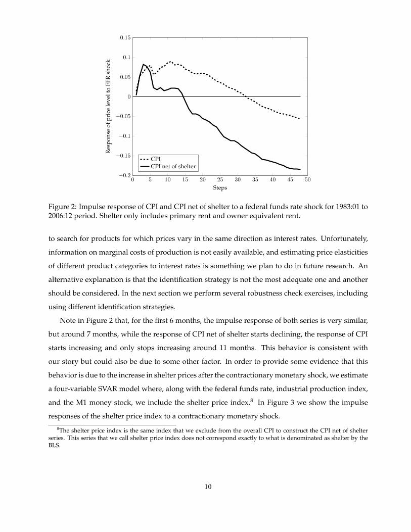
Figure 2 summarizes our main result. In this figure we show the impulse response to a positive

federal funds rate shock of overall CPI and CPI net of shelter.

The impulse response of overall CPI to an increase of the federal funds rate corresponds to what

is perceived as being puzzling and at odds with economic theory. After an increase of the interest

rate, CPI is above the baseline level for more than 30 months. In the the case where we use CPI net

of shelter, we still observe a period of around 14 months where CPI is still above zero, but after 4 to

5 months the level is significantly lower than overall CPI and after 14 months it actually becomes

negative, as would be expected. The reason why even when we use CPI net of shelter we still

observe an initial period where CPI is above zero after a contractionary monetary shock is not easy

to explain. This initial behavior could be explained by the theory of the cost channel of monetary

policy. It is also possible that there are other products for which demand increases after a negative

interest rate shock. In order to test the first hypothesis we would need some information about

the evolution of marginal costs of production, while to test the second hypothesis we would have

9

0 5 10 15 20 25 30 35 40 45 50−0.2

−0.15

−0.1

−0.05

0

0.05

0.1

0.15

Steps

Res

pons

eof

pric

ele

velt

oFF

Rsh

ock

CPICPI net of shelter

Figure 2: Impulse response of CPI and CPI net of shelter to a federal funds rate shock for 1983:01 to2006:12 period. Shelter only includes primary rent and owner equivalent rent.

to search for products for which prices vary in the same direction as interest rates. Unfortunately,

information on marginal costs of production is not easily available, and estimating price elasticities

of different product categories to interest rates is something we plan to do in future research. An

alternative explanation is that the identification strategy is not the most adequate one and another

should be considered. In the next section we perform several robustness check exercises, including

using different identification strategies.

Note in Figure 2 that, for the first 6 months, the impulse response of both series is very similar,

but around 7 months, while the response of CPI net of shelter starts declining, the response of CPI

starts increasing and only stops increasing around 11 months. This behavior is consistent with

our story but could also be due to some other factor. In order to provide some evidence that this

behavior is due to the increase in shelter prices after the contractionary monetary shock, we estimate

a four-variable SVAR model where, along with the federal funds rate, industrial production index,

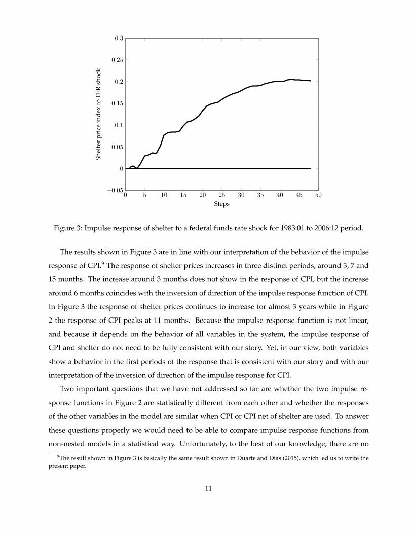
and the M1 money stock, we include the shelter price index.8 In Figure 3 we show the impulse

responses of the shelter price index to a contractionary monetary shock.

8The shelter price index is the same index that we exclude from the overall CPI to construct the CPI net of shelterseries. This series that we call shelter price index does not correspond exactly to what is denominated as shelter by theBLS.

10

0 5 10 15 20 25 30 35 40 45 50−0.05

0

0.05

0.1

0.15

0.2

0.25

0.3

Steps

Shel

ter

pric

ein

dex

toFF

Rsh

ock

Figure 3: Impulse response of shelter to a federal funds rate shock for 1983:01 to 2006:12 period.

The results shown in Figure 3 are in line with our interpretation of the behavior of the impulse

response of CPI.9 The response of shelter prices increases in three distinct periods, around 3, 7 and

15 months. The increase around 3 months does not show in the response of CPI, but the increase

around 6 months coincides with the inversion of direction of the impulse response function of CPI.

In Figure 3 the response of shelter prices continues to increase for almost 3 years while in Figure

2 the response of CPI peaks at 11 months. Because the impulse response function is not linear,

and because it depends on the behavior of all variables in the system, the impulse response of

CPI and shelter do not need to be fully consistent with our story. Yet, in our view, both variables

show a behavior in the first periods of the response that is consistent with our story and with our

interpretation of the inversion of direction of the impulse response for CPI.

Two important questions that we have not addressed so far are whether the two impulse re-

sponse functions in Figure 2 are statistically different from each other and whether the responses

of the other variables in the model are similar when CPI or CPI net of shelter are used. To answer

these questions properly we would need to be able to compare impulse response functions from

non-nested models in a statistical way. Unfortunately, to the best of our knowledge, there are no

9The result shown in Figure 3 is basically the same result shown in Duarte and Dias (2015), which led us to write thepresent paper.

11

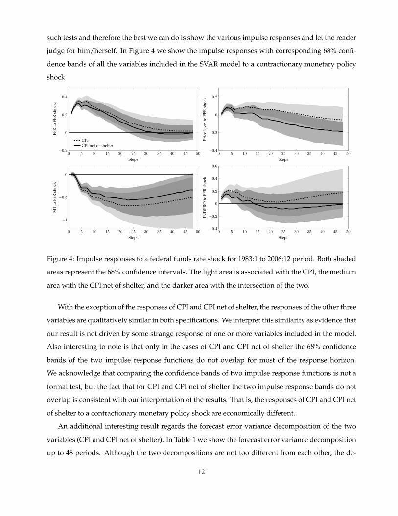
such tests and therefore the best we can do is show the various impulse responses and let the reader

judge for him/herself. In Figure 4 we show the impulse responses with corresponding 68% confi-

dence bands of all the variables included in the SVAR model to a contractionary monetary policy

shock.

0 5 10 15 20 25 30 35 40 45 50−0.2

0

0.2

0.4

Steps

FFR

toFF

Rsh

ock

CPICPI net of shelter

0 5 10 15 20 25 30 35 40 45 50−0.4

−0.2

0

0.2

Steps

Pric

ele

velt

oFF

Rsh

ock

0 5 10 15 20 25 30 35 40 45 50−0.4

−0.2

0

0.2

0.4

0.6

Steps

IND

PRO

toFF

Rsh

ock

0 5 10 15 20 25 30 35 40 45 50

−1

−0.5

0

Steps

M1

toFF

Rsh

ock

Figure 4: Impulse responses to a federal funds rate shock for 1983:1 to 2006:12 period. Both shaded

areas represent the 68% confidence intervals. The light area is associated with the CPI, the medium

area with the CPI net of shelter, and the darker area with the intersection of the two.

With the exception of the responses of CPI and CPI net of shelter, the responses of the other three

variables are qualitatively similar in both specifications. We interpret this similarity as evidence that

our result is not driven by some strange response of one or more variables included in the model.

Also interesting to note is that only in the cases of CPI and CPI net of shelter the 68% confidence

bands of the two impulse response functions do not overlap for most of the response horizon.

We acknowledge that comparing the confidence bands of two impulse response functions is not a

formal test, but the fact that for CPI and CPI net of shelter the two impulse response bands do not

overlap is consistent with our interpretation of the results. That is, the responses of CPI and CPI net

of shelter to a contractionary monetary policy shock are economically different.

An additional interesting result regards the forecast error variance decomposition of the two

variables (CPI and CPI net of shelter). In Table 1 we show the forecast error variance decomposition

up to 48 periods. Although the two decompositions are not too different from each other, the de-

12

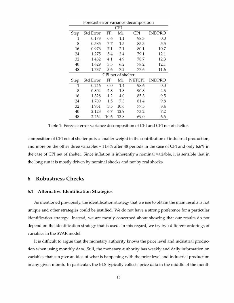
Forecast error variance decompositionCPI

Step Std Error FF M1 CPI INDPRO1 0.173 0.6 1.1 98.3 0.08 0.585 7.7 1.5 85.3 5.5

16 0.976 7.1 2.1 80.1 10.724 1.275 5.4 3.4 79.1 12.132 1.482 4.1 4.9 78.7 12.340 1.629 3.5 6.2 78.2 12.148 1.737 3.6 7.2 77.6 11.6

CPI net of shelterStep Std Error FF M1 NETCPI INDPRO

1 0.246 0.0 1.4 98.6 0.08 0.804 2.8 1.8 90.8 4.6

16 1.328 1.2 4.0 85.3 9.524 1.709 1.5 7.3 81.4 9.832 1.951 3.5 10.6 77.5 8.440 2.123 6.7 12.9 73.2 7.248 2.264 10.6 13.8 69.0 6.6

Table 1: Forecast error variance decomposition of CPI and CPI net of shelter.

composition of CPI net of shelter puts a smaller weight in the contribution of industrial production,

and more on the other three variables – 11.6% after 48 periods in the case of CPI and only 6.6% in

the case of CPI net of shelter. Since inflation is inherently a nominal variable, it is sensible that in

the long run it is mostly driven by nominal shocks and not by real shocks.

6 Robustness Checks

6.1 Alternative Identification Strategies

As mentioned previously, the identification strategy that we use to obtain the main results is not

unique and other strategies could be justified. We do not have a strong preference for a particular

identification strategy. Instead, we are mostly concerned about showing that our results do not

depend on the identification strategy that is used. In this regard, we try two different orderings of

variables in the SVAR model.

It is difficult to argue that the monetary authority knows the price level and industrial produc-

tion when using monthly data. Still, the monetary authority has weekly and daily information on

variables that can give an idea of what is happening with the price level and industrial production

in any given month. In particular, the BLS typically collects price data in the middle of the month

13

while the Federal Open Market Committee (FOMC) meets either in the middle or at the end of the

month. We present here two different orderings: one where the monetary authority observes con-

temporaneously industrial production and the price level, as in Christiano et al. (1996), and one

where it just observes the price level. Results of the these two alternative identification strategies

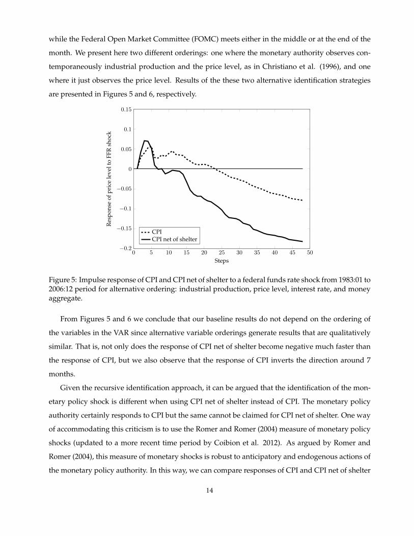
are presented in Figures 5 and 6, respectively.

0 5 10 15 20 25 30 35 40 45 50−0.2

−0.15

−0.1

−0.05

0

0.05

0.1

0.15

Steps

Res

pons

eof

pric

ele

velt

oFF

Rsh

ock

CPICPI net of shelter

Figure 5: Impulse response of CPI and CPI net of shelter to a federal funds rate shock from 1983:01 to2006:12 period for alternative ordering: industrial production, price level, interest rate, and moneyaggregate.

From Figures 5 and 6 we conclude that our baseline results do not depend on the ordering of

the variables in the VAR since alternative variable orderings generate results that are qualitatively

similar. That is, not only does the response of CPI net of shelter become negative much faster than

the response of CPI, but we also observe that the response of CPI inverts the direction around 7

months.

Given the recursive identification approach, it can be argued that the identification of the mon-

etary policy shock is different when using CPI net of shelter instead of CPI. The monetary policy

authority certainly responds to CPI but the same cannot be claimed for CPI net of shelter. One way

of accommodating this criticism is to use the Romer and Romer (2004) measure of monetary policy

shocks (updated to a more recent time period by Coibion et al. 2012). As argued by Romer and

Romer (2004), this measure of monetary shocks is robust to anticipatory and endogenous actions of

the monetary policy authority. In this way, we can compare responses of CPI and CPI net of shelter

14

0 5 10 15 20 25 30 35 40 45 50−0.25

−0.2

−0.15

−0.1

−0.05

0

0.05

0.1

Steps

Res

pons

eof

pric

ele

velt

oFF

Rsh

ock

CPICPI net of shelter

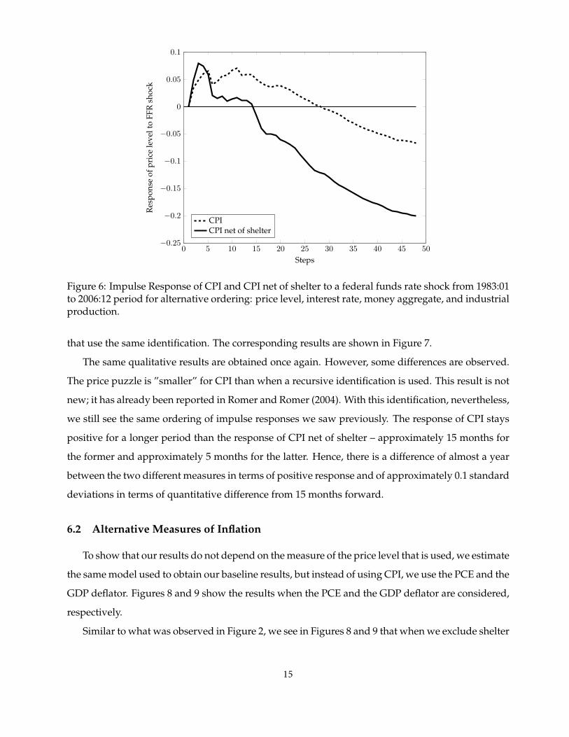
Figure 6: Impulse Response of CPI and CPI net of shelter to a federal funds rate shock from 1983:01to 2006:12 period for alternative ordering: price level, interest rate, money aggregate, and industrialproduction.

that use the same identification. The corresponding results are shown in Figure 7.

The same qualitative results are obtained once again. However, some differences are observed.

The price puzzle is ”smaller” for CPI than when a recursive identification is used. This result is not

new; it has already been reported in Romer and Romer (2004). With this identification, nevertheless,

we still see the same ordering of impulse responses we saw previously. The response of CPI stays

positive for a longer period than the response of CPI net of shelter – approximately 15 months for

the former and approximately 5 months for the latter. Hence, there is a difference of almost a year

between the two different measures in terms of positive response and of approximately 0.1 standard

deviations in terms of quantitative difference from 15 months forward.

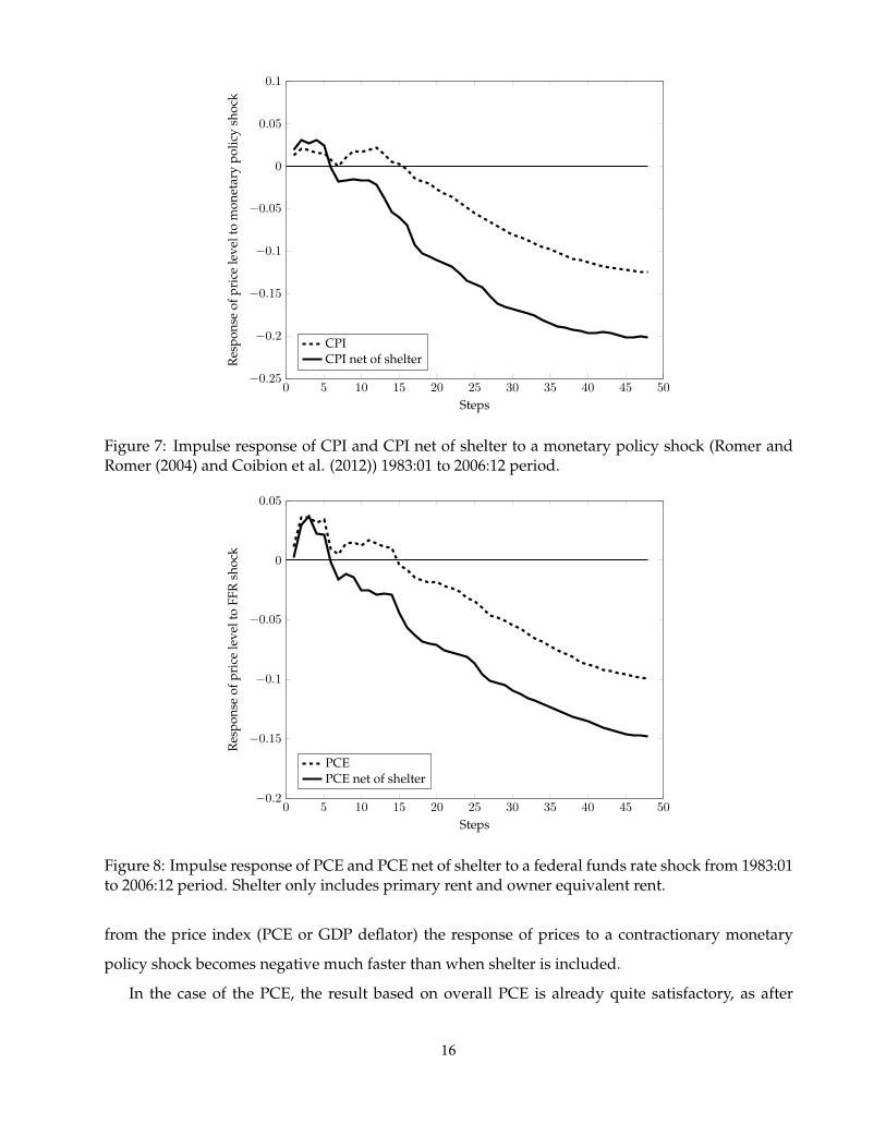
6.2 Alternative Measures of Inflation

To show that our results do not depend on the measure of the price level that is used, we estimate

the same model used to obtain our baseline results, but instead of using CPI, we use the PCE and the

GDP deflator. Figures 8 and 9 show the results when the PCE and the GDP deflator are considered,

respectively.

Similar to what was observed in Figure 2, we see in Figures 8 and 9 that when we exclude shelter

15

0 5 10 15 20 25 30 35 40 45 50−0.25

−0.2

−0.15

−0.1

−0.05

0

0.05

0.1

Steps

Res

pons

eof

pric

ele

velt

om

onet

ary

polic

ysh

ock

CPICPI net of shelter

Figure 7: Impulse response of CPI and CPI net of shelter to a monetary policy shock (Romer andRomer (2004) and Coibion et al. (2012)) 1983:01 to 2006:12 period.

0 5 10 15 20 25 30 35 40 45 50−0.2

−0.15

−0.1

−0.05

0

0.05

Steps

Res

pons

eof

pric

ele

velt

oFF

Rsh

ock

PCEPCE net of shelter

Figure 8: Impulse response of PCE and PCE net of shelter to a federal funds rate shock from 1983:01to 2006:12 period. Shelter only includes primary rent and owner equivalent rent.

from the price index (PCE or GDP deflator) the response of prices to a contractionary monetary

policy shock becomes negative much faster than when shelter is included.

In the case of the PCE, the result based on overall PCE is already quite satisfactory, as after

16

0 1 2 3 4 5 6 7 8 9 10 11 12 13−0.3

−0.25

−0.2

−0.15

−0.1

−0.05

0

0.05

0.1

Steps

Res

pons

eof

pric

ele

velt

oFF

Rsh

ock

GDP deflatorGDP deflator net of shelter

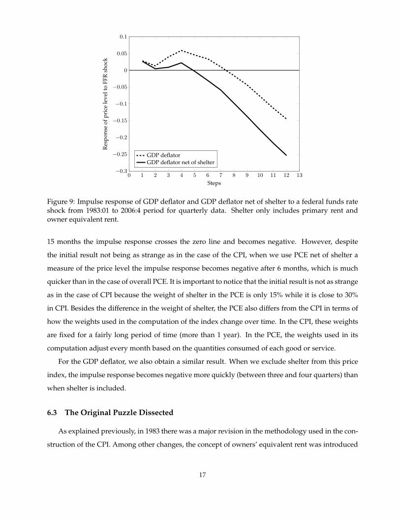
Figure 9: Impulse response of GDP deflator and GDP deflator net of shelter to a federal funds rateshock from 1983:01 to 2006:4 period for quarterly data. Shelter only includes primary rent andowner equivalent rent.

15 months the impulse response crosses the zero line and becomes negative. However, despite

the initial result not being as strange as in the case of the CPI, when we use PCE net of shelter a

measure of the price level the impulse response becomes negative after 6 months, which is much

quicker than in the case of overall PCE. It is important to notice that the initial result is not as strange

as in the case of CPI because the weight of shelter in the PCE is only 15% while it is close to 30%

in CPI. Besides the difference in the weight of shelter, the PCE also differs from the CPI in terms of

how the weights used in the computation of the index change over time. In the CPI, these weights

are fixed for a fairly long period of time (more than 1 year). In the PCE, the weights used in its

computation adjust every month based on the quantities consumed of each good or service.

For the GDP deflator, we also obtain a similar result. When we exclude shelter from this price

index, the impulse response becomes negative more quickly (between three and four quarters) than

when shelter is included.

6.3 The Original Puzzle Dissected

As explained previously, in 1983 there was a major revision in the methodology used in the con-

struction of the CPI. Among other changes, the concept of owners’ equivalent rent was introduced

17

and the cost of home ownership item was removed from the index. This change brings naturally

the investigation of the pre-1983 period as a robustness check. Figure 10 shows results based on the

sample used in the original article as well as results for two sub-samples – before and after 1983.

Given our previous discussion, it would be expected that the price puzzle would be ”worse” af-

ter 1983 because that corresponds to the period with a higher weight of shelter. This hypothesis

is confirmed in Figure 10, where it can be seen that the CPI impulse response function is positive

for more than 48 months. Also interesting is that only in the post-1983 sample is a change of di-

rection of the impulse response function observed. This inversion of direction also takes place at

around 8 months, and the impulse response stabilizes around month 13/14. Regarding the pre-1983

sub-period we observe a slightly ”smaller” puzzle than the original.

0 5 10 15 20 25 30 35 40 45 50−0.4

−0.3

−0.2

−0.1

0

0.1

0.2

0.3

Steps

Res

pons

eof

CPI

toFF

Rsh

ock

1960:1-1992:12 original puzzle1983:1-1992:121960:1-1982:12

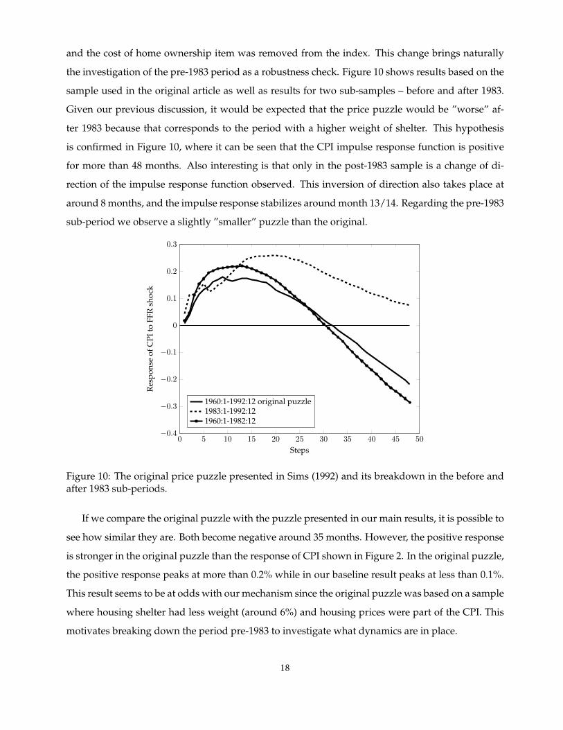
Figure 10: The original price puzzle presented in Sims (1992) and its breakdown in the before andafter 1983 sub-periods.

If we compare the original puzzle with the puzzle presented in our main results, it is possible to

see how similar they are. Both become negative around 35 months. However, the positive response

is stronger in the original puzzle than the response of CPI shown in Figure 2. In the original puzzle,

the positive response peaks at more than 0.2% while in our baseline result peaks at less than 0.1%.

This result seems to be at odds with our mechanism since the original puzzle was based on a sample

where housing shelter had less weight (around 6%) and housing prices were part of the CPI. This

motivates breaking down the period pre-1983 to investigate what dynamics are in place.

18

0 5 10 15 20 25 30 35 40 45 50−7

−6

−5

−4

−3

−2

−1

0

1

2

3·10−3

Steps

Res

pons

eof

CPI

toFF

Rsh

ock

1960:1-1969:121970:1-1982:121970:1-1982:12 with comm. price

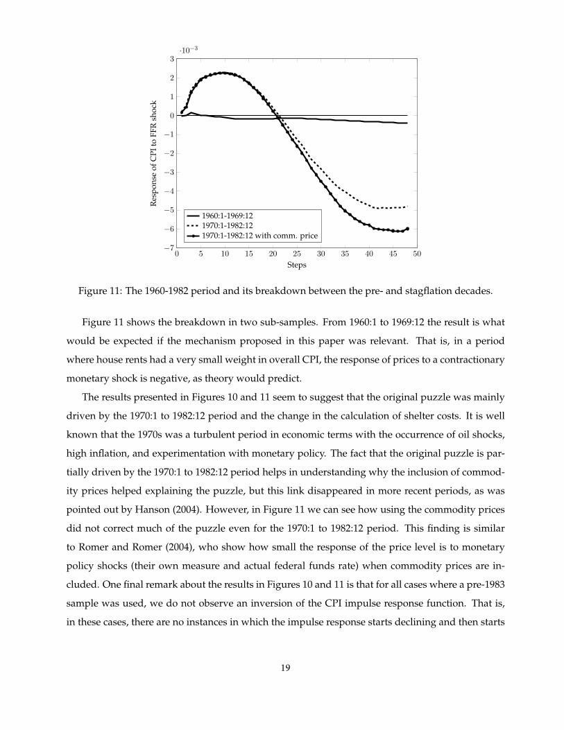
Figure 11: The 1960-1982 period and its breakdown between the pre- and stagflation decades.

Figure 11 shows the breakdown in two sub-samples. From 1960:1 to 1969:12 the result is what

would be expected if the mechanism proposed in this paper was relevant. That is, in a period

where house rents had a very small weight in overall CPI, the response of prices to a contractionary

monetary shock is negative, as theory would predict.

The results presented in Figures 10 and 11 seem to suggest that the original puzzle was mainly

driven by the 1970:1 to 1982:12 period and the change in the calculation of shelter costs. It is well

known that the 1970s was a turbulent period in economic terms with the occurrence of oil shocks,

high inflation, and experimentation with monetary policy. The fact that the original puzzle is par-

tially driven by the 1970:1 to 1982:12 period helps in understanding why the inclusion of commod-

ity prices helped explaining the puzzle, but this link disappeared in more recent periods, as was

pointed out by Hanson (2004). However, in Figure 11 we can see how using the commodity prices

did not correct much of the puzzle even for the 1970:1 to 1982:12 period. This finding is similar

to Romer and Romer (2004), who show how small the response of the price level is to monetary

policy shocks (their own measure and actual federal funds rate) when commodity prices are in-

cluded. One final remark about the results in Figures 10 and 11 is that for all cases where a pre-1983

sample was used, we do not observe an inversion of the CPI impulse response function. That is,

in these cases, there are no instances in which the impulse response starts declining and then starts

19

increasing again, as was the case for impulse responses based on post-1983 samples.

7 Alternative Explanations of the Price Puzzle

As discussed in the introduction, there are several explanations for the price puzzle, each with

its own merits. We do not want to discuss whether our explanation is better than existing ones nor

take a stand on which explanation is our preferred one. Instead, we want to see how our explanation

fits with existing ones. To do so, we replicate some of the leading explanations of the price puzzle

incorporating our idea. We choose four alternative explanations: 1) exclusion of a measure of output

gap - Giordani (2004); 2) exclusion of forward looking variables - Brissimis and Magginas (2006); 3)

insufficient controlling for other variables used in the information set of the central banker - FAVAR

model of Bernanke, Boiving and Eliasz (2005); 4) theory based sign restriction method of Uhligh

(2005).10

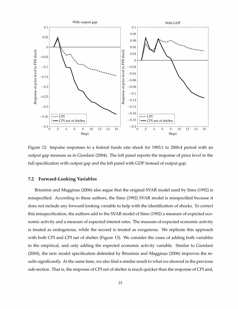
7.1 Output Gap

Giordani (2004) argues that the SVAR model used by Sims (1992) is misspecified, and this mis-

specification lead to a spurious price puzzle. The source of the misspecification is the inclusion of a

measure of GDP (or industrial production) instead of using a measure of output gap. In Figure 12

we show the impulse response function of CPI and CPI net of a shelter to a contractionary monetary

policy shock in the context of a model with output gap (left panel) and with GDP (right panel). As

is visible in Figure 12, the SVAR model with output gap delivers results where there is almost no

price puzzle for both CPI and CPI net of shelter, but it also shows that CPI net of shelter responds

more negatively than CPI to the same monetary shock. In the case of the SVAR model that uses

GDP, the response of CPI is always positive for the first four years, while the response of CPI net

of shelter becomes negative after two years. These results make it very clear that the point made

by Giordani (2004) is important, but the results also show that using the response of inflation to

monetary shocks is quicker than what is implied by the response of CPI. From our discussion in

section 2, the fact that rents increase after a contractionary monetary policy shock does not always

lead to a price puzzle, but the response of CPI is always a combination of two distinct responses:

the response of the shelter and the non-shelter components of CPI.

10To be fair to the author, the main goal of Uhligh (2005) is to study the effects of monetary policy shocks on output,and in order to better identify monetary policy shocks, the author imposes restrictions on the response of prices.

20

0 2 4 6 8 10 12 14 16−0.4

−0.35

−0.3

−0.25

−0.2

−0.15

−0.1

−0.05

0

0.05

0.1

Steps

Res

pons

eof

pric

ele

velt

oFF

Rsh

ock

With output gap

CPICPI net of shelter

0 2 4 6 8 10 12 14 16−0.2

−0.18

−0.16

−0.14

−0.12

−0.1

−0.08

−0.06

−0.04

−0.02

0

0.02

0.04

0.06

0.08

0.1

Steps

Res

pons

eof

pric

ele

velt

oFF

Rsh

ock

With GDP

CPICPI net of shelter

Figure 12: Impulse responses to a federal funds rate shock for 1983:1 to 2006:4 period with an

output gap measure as in Giordani (2004). The left panel reports the response of price level to the

full specification with output gap and the left panel with GDP instead of output gap.

7.2 Forward-Looking Variables

Brissimis and Magginas (2006) also argue that the original SVAR model used by Sims (1992) is

misspecified. According to these authors, the Sims (1992) SVAR model is misspecified because it

does not include any forward-looking variable to help with the identification of shocks. To correct

this misspecification, the authors add to the SVAR model of Sims (1992) a measure of expected eco-

nomic activity and a measure of expected interest rates. The measure of expected economic activity

is treated as endogenous, while the second is treated as exogenous. We replicate this approach

with both CPI and CPI net of shelter (Figure 13). We consider the cases of adding both variables

to the empirical, and only adding the expected economic activity variable. Similar to Giordani

(2004), the new model specification defended by Brissimis and Magginas (2006) improves the re-

sults significantly. At the same time, we also find a similar result to what we showed in the previous

sub-section. That is, the response of CPI net of shelter is much quicker than the response of CPI and,

21

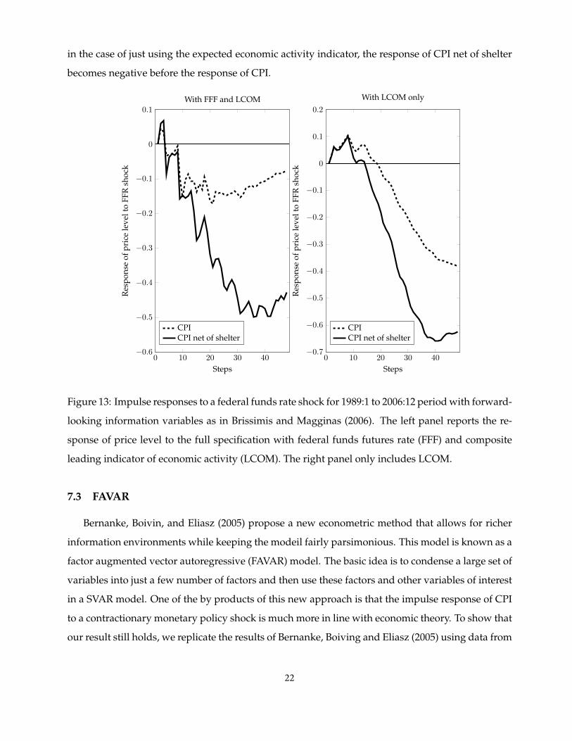
in the case of just using the expected economic activity indicator, the response of CPI net of shelter

becomes negative before the response of CPI.

0 10 20 30 40−0.6

−0.5

−0.4

−0.3

−0.2

−0.1

0

0.1

Steps

Res

pons

eof

pric

ele

velt

oFF

Rsh

ock

With FFF and LCOM

CPICPI net of shelter

0 10 20 30 40−0.7

−0.6

−0.5

−0.4

−0.3

−0.2

−0.1

0

0.1

0.2

Steps

Res

pons

eof

pric

ele

velt

oFF

Rsh

ock

With LCOM only

CPICPI net of shelter

Figure 13: Impulse responses to a federal funds rate shock for 1989:1 to 2006:12 period with forward-

looking information variables as in Brissimis and Magginas (2006). The left panel reports the re-

sponse of price level to the full specification with federal funds futures rate (FFF) and composite

leading indicator of economic activity (LCOM). The right panel only includes LCOM.

7.3 FAVAR

Bernanke, Boivin, and Eliasz (2005) propose a new econometric method that allows for richer

information environments while keeping the modeil fairly parsimonious. This model is known as a

factor augmented vector autoregressive (FAVAR) model. The basic idea is to condense a large set of

variables into just a few number of factors and then use these factors and other variables of interest

in a SVAR model. One of the by products of this new approach is that the impulse response of CPI

to a contractionary monetary policy shock is much more in line with economic theory. To show that

our result still holds, we replicate the results of Bernanke, Boiving and Eliasz (2005) using data from

22

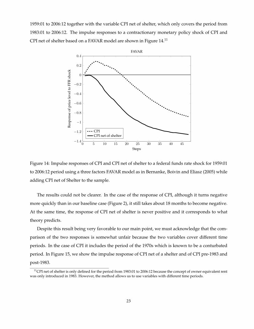
1959:01 to 2006:12 together with the variable CPI net of shelter, which only covers the period from

1983:01 to 2006:12. The impulse responses to a contractionary monetary policy shock of CPI and

CPI net of shelter based on a FAVAR model are shown in Figure 14.11

0 5 10 15 20 25 30 35 40 45−1.4

−1.2

−1

−0.8

−0.6

−0.4

−0.2

0

0.2

0.4

Steps

Res

pons

eof

pric

ele

velt

oFF

Rsh

ock

FAVAR

CPICPI net of shelter

Figure 14: Impulse responses of CPI and CPI net of shelter to a federal funds rate shock for 1959:01

to 2006:12 period using a three factors FAVAR model as in Bernanke, Boivin and Eliasz (2005) while

adding CPI net of Shelter to the sample.

The results could not be clearer. In the case of the response of CPI, although it turns negative

more quickly than in our baseline case (Figure 2), it still takes about 18 months to become negative.

At the same time, the response of CPI net of shelter is never positive and it corresponds to what

theory predicts.

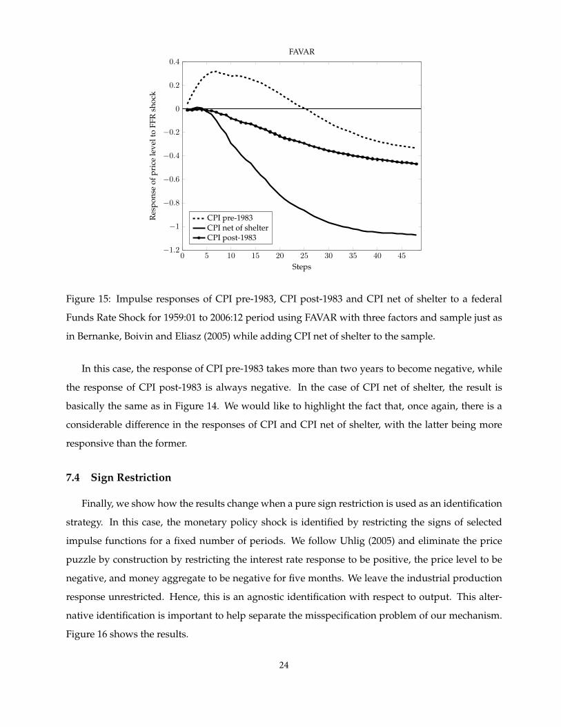
Despite this result being very favorable to our main point, we must acknowledge that the com-

parison of the two responses is somewhat unfair because the two variables cover different time

periods. In the case of CPI it includes the period of the 1970s which is known to be a conturbated

period. In Figure 15, we show the impulse response of CPI net of a shelter and of CPI pre-1983 and

post-1983.

11CPI net of shelter is only defined for the period from 1983:01 to 2006:12 because the concept of owner equivalent rentwas only introduced in 1983. However, the method allows us to use variables with different time periods.

23

0 5 10 15 20 25 30 35 40 45−1.2

−1

−0.8

−0.6

−0.4

−0.2

0

0.2

0.4

Steps

Res

pons

eof

pric

ele

velt

oFF

Rsh

ock

FAVAR

CPI pre-1983CPI net of shelterCPI post-1983

Figure 15: Impulse responses of CPI pre-1983, CPI post-1983 and CPI net of shelter to a federal

Funds Rate Shock for 1959:01 to 2006:12 period using FAVAR with three factors and sample just as

in Bernanke, Boivin and Eliasz (2005) while adding CPI net of shelter to the sample.

In this case, the response of CPI pre-1983 takes more than two years to become negative, while

the response of CPI post-1983 is always negative. In the case of CPI net of shelter, the result is

basically the same as in Figure 14. We would like to highlight the fact that, once again, there is a

considerable difference in the responses of CPI and CPI net of shelter, with the latter being more

responsive than the former.

7.4 Sign Restriction

Finally, we show how the results change when a pure sign restriction is used as an identification

strategy. In this case, the monetary policy shock is identified by restricting the signs of selected

impulse functions for a fixed number of periods. We follow Uhlig (2005) and eliminate the price

puzzle by construction by restricting the interest rate response to be positive, the price level to be

negative, and money aggregate to be negative for five months. We leave the industrial production

response unrestricted. Hence, this is an agnostic identification with respect to output. This alter-

native identification is important to help separate the misspecification problem of our mechanism.

Figure 16 shows the results.

24

0 5 10 15 20 25 30 35 40 45 50−0.5

−0.45

−0.4

−0.35

−0.3

−0.25

−0.2

−0.15

−0.1

−0.05

0

Steps

Res

pons

eof

pric

ele

velt

oFF

Rsh

ock

CPICPI net of shelter

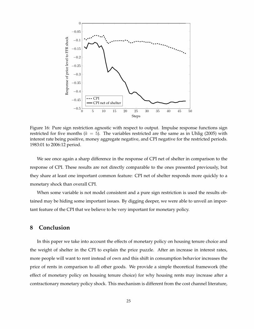
Figure 16: Pure sign restriction agnostic with respect to output. Impulse response functions signrestricted for five months (k = 5). The variables restricted are the same as in Uhlig (2005) withinterest rate being positive, money aggregate negative, and CPI negative for the restricted periods.1983:01 to 2006:12 period.

We see once again a sharp difference in the response of CPI net of shelter in comparison to the

response of CPI. These results are not directly comparable to the ones presented previously, but

they share at least one important common feature: CPI net of shelter responds more quickly to a

monetary shock than overall CPI.

When some variable is not model consistent and a pure sign restriction is used the results ob-

tained may be hiding some important issues. By digging deeper, we were able to unveil an impor-

tant feature of the CPI that we believe to be very important for monetary policy.

8 Conclusion

In this paper we take into account the effects of monetary policy on housing tenure choice and

the weight of shelter in the CPI to explain the price puzzle. After an increase in interest rates,

more people will want to rent instead of own and this shift in consumption behavior increases the

price of rents in comparison to all other goods. We provide a simple theoretical framework (the

effect of monetary policy on housing tenure choice) for why housing rents may increase after a

contractionary monetary policy shock. This mechanism is different from the cost channel literature,

25

and our empirical results suggest that it is relevant in explaining the price puzzle. Our results are

qualitatively robust to different identification strategies, measures of inflation, sample periods, and

they compare well against alternative explanations.

In our opinion, these results would be interesting on their own, but they may be significantly

more far-reaching than just explaining the price puzzle. While providing a possible explanation

for the price puzzle, we showed that, when we exclude shelter from the CPI, inflation seems to be

much less persistent than previously thought. More generally, the results of this paper highlight the

importance of measuring inflation in a theoretically consistent way to better separate price changes

cause by inflation from price changes caused by relative price changes.

References

Barth, Marvin J., and Ramey, Valerie A., 2001, “The Cost Channel of Monetary Transmission,”

NBER Macroeconomics Annual.

Bernanke, Ben S., Boivin, Jean, and Eliasz, Piotr, 2005, “Measuring the Effects of Mone-

tary Policy: A Factor-Augmented Vector Autoregressive (FAVAR) Approach,” The Quarterly

Journal of Economics, Volume 120 (1), 387-422.

BLS, 2009, “How the CPI measures price change of Owner’s equivalent rent of primary resi-

dence (OER) and Rent of primary residence (Rent), ” Bureau of Labor Statistics.

Brissimis, Sophocles N., and Magginas, Nicholas S., 2006, “Forward-Looking Information in

VAR Models and the Price Puzzle,” Journal of Monetary Economics, Volume 53(6), pp. 1225-

1234.

Christiano, Lawrence J., Eichenbaum, Martin, and Evans, Charles, 1996, “The Effects of Mon-

etary Policy Shocks: Evidence from the Flow of Funds,” Review of Economics and Statistics,

Volume 78(1), pp. 16-34.

Church, Jonathan D., 2014, “Explaining the 30-year shift in consumer expenditures from com-

modities to services, 1982-2012.,” Monthly Labor Review, April.

Clark, Todd E., 2001, “Comparing Measures of Core Inflation,” Economic Review, second quar-

ter, pp. 5-31.

26

Coibion, Olivier, Gorodnichenko, Yuriy, Kueng, Lorenz, and Silvia, John, 2012, “Innocent

Bystanders? Monetary Policy and Inequality in the U.S.,” NBER Working Paper No. 18170

Duarte, Joao B. and Dias, Daniel A., 2015, “Housing, Inflation and Monetary Policy in the

Business Cycle: What Do Housing Rents Have to Say?,”mimeo, UIUC.

Gillingham, Robert, and Lane, Walter, 1982, “Changing the Treatment of Shelter Costs for

Homeowners in the CPI, ” Montlhy Labor Review, June, pp. 9-14.

Giordani, Paolo, 2004, “An Alternative Explanation of the Price Puzzle, ” Journal of Monetary

Economics, Volume 51, pp. 1271-1296.

Hanson, Michael S., 2004, “The ’Price Puzzle’ Reconsidered,” Journal of Monetary Economics,

Volume 51, pp. 1385-1413.

Henzel, Steffen, Hlsewig, Oliver, Mayer, Eric, and Wollmershuser, Timo, 2009, “The price

puzzle revisited: Can the Cost Channel Explain a Rise in Inflation after a Monetary Policy

Shock?,” Journal of Macroeconomics, Volume 31(2), pp. 268-289.

Rabanal, Pau, 2006, “Does inflation increase after a monetary policy tightening? Answers

based on an estimated DSGE model,” Journal of Economics Dynamics Control, Volume 31,

pp. 906-937.

Romer, Christina D., and David H. Romer., 2004, “A New Measure of Monetary Shocks:

Derivation and Implications,” American Economic Review, Volume 94(4), pp. 1055-1084.

Sims, Chris A., 1992, “Interpreting the macroeconomic time series facts: the effects of mone-

tary policy,” European Economic Review, Volume 36 (5), pp. 975-1000.

Uhlig, Harald, 2005, “What are the effects of monetary policy on output? Results from an

agnostic identification procedure,” Journal of Monetary Economics, Volume 52, pp. 381-419.

27