AE Kaiser Effect and Electromagnetic Emission in The - NDT.net

DEGREE PROJECT IN MATERIALS SCIENCE AND ENGINEERING, SECOND CYCLE, 30 CREDITS STOCKHOLM, SWEDEN 2018
The Effect of Electromagnetic
Stirring and Flow Control Devices
on Eight-Strand Tundish
Performance
BINTANG BERGAS CENDEKIA
KTH ROYAL INSTITUTE OF TECHNOLOGY SCHOOL OF INDUSTRIAL ENGINEERING AND MANAGEMENT

i
ABSTRACT The strand similarity and inclusion removal capability are two critical parameters to
measure the performance of multi-strand tundish in clean steel production. In this work, the
effect of two flow regulators, i.e., Flow Control Devices (FCD) and Electromagnetic Stirring
(EMS) on eight-strand tundish performance have been investigated by establishing a water
model and conducting numerical simulations of water model. The water model was focused on
revealing the effect of stirring while the simulation was employed to investigate the effect of
two FCDs, namely baffle wall and turbo-stopper. The analysis of strand similarity and inclusion
removal were conducted by analyzing flow characteristics derived from Combined Model of
Residence Time Distribution (RTD) curve and observing the flow movement in the tundish
model. In addition, the tundish capability to remove inclusions was also studied by injecting
inclusion particles using Discrete Phase Model (DPM) in ANSYS Fluent. Experiment results
cause the Combined Model needs to be modified. This modification was employed when
analyzing tundish configuration involving stirring. By using the modified Combined Model,
the stirring can significantly increase the well-mix volume to almost 100% as it annihilates
dead zone. The stirring also increases the similarity between strands and makes the RTD curve
more similar to ideal mixing curve. However, the problem of short-circuiting flow need to be
solved and care should be taken into consideration regarding the selection of stirring direction
as well as bath surface condition when implementing EMS in reality. The simulation results
show that the addition of baffle wall and turbo-stopper are beneficial to improve mixing as well
as to avoid the short-circuiting flow. Furthermore, compared to individual FCD, the
combination of baffle wall and turbo-stopper results in the best performance to remove
inclusions by providing surface-directed flow and generating a higher plug flow.
Keywords: multi-strand tundish, strand similarity, flow characteristic, EMS, flow control
device

ii
PREFACE
I would like to express my gratitude to my supervisor at KTH, Mikael Ersson for all his
help and guidance throughout this project. I also want to thank Lidong Teng and Hongliang
Yang as my supervisor in ABB Metallurgy for all their support and advice during my time in
ABB Metallurgy. Finally, I want to thank LPDP (Indonesia Endowment Fund for Education)
for giving me scholarship during my master degree education in KTH.

iii
TABLE OF CONTENT
1 INTRODUCTION ................................................................................................................... 1
2 TUNDISH METALLURGY AND PHYSICAL MODELLING .......................................................... 3
2.1 Tundish Role in Clean Steel Production ..................................................................... 3
2.2 Non-Metallic Inclusion Removal in the tundish ......................................................... 4
2.3 Current Strategies on Inclusion Removal in the tundish ............................................. 4
2.4 Tundish Flow............................................................................................................... 5
2.4.1 Tundish Flow Characterization ............................................................................ 5
2.4.2 Tundish Flow Problem ......................................................................................... 6
2.5 Tundish Performance Measurement............................................................................ 6
2.6 Residence Time Distribution Experiment ................................................................... 7
2.6.1 Tracer Injection Method ...................................................................................... 7
2.6.2 Dimensionless C-Curve ....................................................................................... 8
2.7 Flow Characterization Calculation .............................................................................. 9
2.7.1 RTD curve of Plug flow ....................................................................................... 9
2.7.2 RTD curve of Well-Mixed Volume ................................................................... 10
2.7.3 Combined Model ............................................................................................... 10
2.7.4 Plug Volume Fraction ........................................................................................ 11
2.7.5 Dead Volume Definition .................................................................................... 11
2.7.6 Dead Volume Fraction ....................................................................................... 12
2.7.7 Well-Mixed Volume Fraction ............................................................................ 13
2.7.8 Multi-strand Tundish Model .............................................................................. 13
2.7.9 Strand Similarity ................................................................................................ 14
2.8 Tundish Water Model Criteria .................................................................................. 14
2.8.1 Geometric Similarity .......................................................................................... 14
2.8.2 Dynamic Similarity Consideration .................................................................... 15
2.9 Multi-strand tundish problem .................................................................................... 16
2.10 Electromagnetic Stirring Technology .................................................................... 17
3 BASIC THEORY OF NUMERICAL MODELLING .................................................................... 18
3.1 Governing Equations ................................................................................................. 18
3.1.1 Conservation of Mass ........................................................................................ 18
3.1.2 Conservation of Momentum .............................................................................. 18
3.1.3 Species Transport Conservation ........................................................................ 18
3.1.4 Discrete Phase Model (DPM) ............................................................................ 19
3.2 Turbulence Model ..................................................................................................... 19
3.2.1 The Reynold Average Navier Stokes (RANS) model ....................................... 19
3.2.2 The realizable 𝒌−∈ method ............................................................................... 20
3.2.3 Law of the wall and Near Wall-Treatment ........................................................ 20

iv
4 EXPERIMENT SETUP .......................................................................................................... 21
4.1 Model selection ......................................................................................................... 21
4.2 Similarity Consideration ........................................................................................... 22
4.3 Experimental Tools design ........................................................................................ 22
4.3.1 General Setup : Material and – Scale consideration .......................................... 22
4.3.2 Water Tank Requirement ................................................................................... 23
4.3.3 Inlet and Outlet Configuration ........................................................................... 23
4.3.4 Turbo-stopper and Baffle wall attachment ........................................................ 23
4.4 Water Pump for Stirring Position .............................................................................. 26
4.4.1 Pump Location-1 ................................................................................................ 26
4.4.2 Pump Location-2 ................................................................................................ 27
4.4.3 Pump Location-3 ................................................................................................ 27
4.5 Experimental Method and Setup ............................................................................... 28
4.5.1 Velocity Mapping .............................................................................................. 28
4.5.2 Flow Behavior Observation ............................................................................... 29
4.5.3 RTD Experiment ................................................................................................ 29
4.5.4 Dye-Color Injection ........................................................................................... 30
4.6 Data Processing Steps of RTD Experiment .............................................................. 30
4.7 Experiment variables ................................................................................................. 31
5 NUMERICAL SIMULATION SETUP ...................................................................................... 33
5.1 Computer specifications ............................................................................................ 33
5.2 Geometry Domain ..................................................................................................... 33
5.3 Simulation Steps ........................................................................................................ 33
5.3.1 Tracer Injection Simulation ............................................................................... 34
5.3.2 Inclusion Injection Simulation ........................................................................... 34
5.4 Simulation List .......................................................................................................... 35
5.5 Assumption and Model Setup ................................................................................... 36
5.6 Meshing ..................................................................................................................... 36
5.7 Convergence Criteria................................................................................................. 37
5.8 Mesh Sensitivity Study ............................................................................................. 38
6 EXPERIMENT RESULTS ...................................................................................................... 40
6.1 Velocity Mapping ...................................................................................................... 40
6.2 Flow Behavior Observation ...................................................................................... 40
6.3 RTD Experiment ....................................................................................................... 42
6.3.1 Repeatability ...................................................................................................... 42
6.3.2 RTD Curve ......................................................................................................... 43
6.3.3 Flow Characteristics........................................................................................... 46
6.4 Dye-Color Injection................................................................................................... 46
7 NUMERICAL SIMULATION RESULT .................................................................................... 50

v
7.1 RTD Curve ................................................................................................................ 50
7.2 Flow Characteristics Calculation .............................................................................. 51
7.3 Flow-related variable Comparison ............................................................................ 51
7.4 Results of Inclusion Injection Simulation ................................................................. 52
8 EXPERIMENT ANALYSIS ............................................................................................ 53
8.1 Velocity Mapping ...................................................................................................... 53
8.2 Analysis of individual strand..................................................................................... 54
8.3 Analysis of Overall Performance of tundish ............................................................. 54
8.3.1 Plug Flow ........................................................................................................... 55
8.3.2 Dead and Well-Mixed Volume .......................................................................... 56
8.3.3 Plug to Dead Zone ratio ..................................................................................... 56
8.4 New Approach of Dead Zone calculation in Stirring Case ....................................... 58
8.4.1 Reason 1: Fast Moving Fluid ............................................................................. 58
8.4.2 Reason 2: Quick Mixing time ............................................................................ 58
8.4.3 Reason 3: Similarity with RTD Curve of Ideal Mix Flow................................. 59
8.4.4 Modified Combined Model................................................................................ 60
8.5 Type of RTD curve in Stirring Case ......................................................................... 61
8.6 Analysis of Overall Performance Using the New Approach .................................... 63
8.7 Strand Similarity ....................................................................................................... 64
8.8 The Similarity with Ideal Mix Curve ........................................................................ 64
8.8.1 Derivation formula ............................................................................................. 67
8.8.2 Analysis of deviation from ideal mix................................................................. 68
8.9 Plug to Well-Mix Volume ratio ................................................................................ 69
8.10 Particle Collision ................................................................................................... 70
8.11 Surface Condition .................................................................................................. 71
8.12 Ethical and Social Aspect Consideration............................................................... 72
9 NUMERICAL SIMULATION ANALYSIS ................................................................................ 73
9.1 Wall Y+ Problem ...................................................................................................... 73
9.2 Validation of CFD Simulation .................................................................................. 73
9.2.1 Validation of Color Tracer Injection .................................................................. 73
9.2.2 Validation of Prediction Regarding Dead Zone Location ................................. 74
9.2.3 Validation of RTD Curve and Flow Characteristics .......................................... 75
9.3 Effect of Baffle wall .................................................................................................. 77
9.4 Effect of Turbo-stopper ............................................................................................. 79
9.5 Dead Zone Comparison ............................................................................................. 81
9.6 Inclusion Injection Simulation .................................................................................. 81
10 CONCLUSION ..................................................................................................................... 83
11 FURTHER STUDY ............................................................................................................... 84
12 REFERENCES ................................................................................................................ 85

1
1 INTRODUCTION
Tundish has become a fundamental component in clean steel production because it acts as
a metallurgical reactor to remove non-metallic inclusions by allowing floatation of non-
metallic inclusion towards the slag on the surface. Besides, tundish can also homogenize the
steel composition and temperature in such a way by providing a proper flow that promotes
floatation of inclusion and sufficient residence time so that the heat and concentration can be
distributed homogeneously to the whole tundish. Thus, the melt flow has become an interesting
parameter for researchers as it is an influencing factor to improve tundish performance [1].
Currently, several tools to adjust the melt flow within the tundish has been developed as
standard practices in casting foundries such as baffles, weird, dam, or turbo-stopper. Those
techniques, which commonly known as flow control devices (FCD), aim to optimize the melt
flow by creating optimum turbulence and mixing within the melt. However, the consideration
of FCD installation becomes more complicated in a multi-strand tundish. The vast amount of
strands lead to increase the tendency of non-homogeneous melt [2]. The melt flowed to the
strand closer to the ladle shroud only needs a shorter time to reach the strand so that it tends to
have a higher temperature and contains more inclusions compared to the melt which flows to
the further strand [3]. The uneven temperature of each strand can also lead to the different cast
steel microstructure [4].
The particular combination of FCD could still be used to overcome the similarity
problem in the multi-strand tundish. Several studies related to the use of FCD in multi-strand
tundish have been conducted by researchers. Zheng and Zhu conducted an experimental study
using a physical model of the ten-strand tundish and they stated that the combination of the
specific design of turbulence inhibitor and baffles could reduce the inclusion as 42% and lead
an evener distribution of inclusion among the strands [5]. This result has a good agreement
with Tomasz and Marek who did the similar study for six-strand tundish by numerical
modelling and industrial measurements. It is concluded that specific design of baffle could
reduce the transient zone in the tundish [6].
Nevertheless, there are some limitations when using FCD in the multi-strand tundish.
Firstly, the multi-strand tundish usually has insufficient working spaces which make
challenging to install several FCD. In addition, the shape and design of FCD are also very case
sensitive [2, 5, 7, 8] which means the selection of flow control devices must involve both of
tundish design and casting parameters. Moreover, the FCD refractory material is also
susceptible to wear during the long practice so that it affects the productivity, quality as well
as the total cost of its implementation. The last, FCD cannot provide the adjustment of flow for
the whole process time.
One of the solutions that could overcome those problems is to use electromagnetic stirring
(EMS) installed on the tundish to control the melt flow. This technology has been developed
by ABB Metallurgy in Västerås, Sweden. One or two EMS which is installed on the side wall
of tundish can provide stirring during the whole casting process thus there is a possibility to
replace or simplify the FCDs using EMS technology. Theoretically, a horizontal stirring
generated in the melt will mix the melt and adjust the melt flow so that the composition and
temperature could be homogenized. From the flexibility point of view, it can be adjusted easily

2
based on the tundish design and the casting process. Furthermore, although the EMS equipment
is more expensive than FCD, the longer lifetime and lower running cost will make the total
cost becomes comparable. All those advantages make this technology seems to be promising
in the future.
However, a comprehensive analysis of the melt flow generated from EMS has not well-
understood due to the lack of studies related to the application of this technology in the tundish
application. Hence, the focus of this work is to investigate the possibility to replace FCD with
EMS in multi-strand tundish application by comparing the flow pattern generated in the tundish
for both cases. The investigation was conducted via physical modelling of eight strand tundish
and numerical modelling of the experiment. The water model experiment was focused on
revealing the effect of stirring while the numerical modelling was employed to investigate the
effect of such FCD. The analysis of flow movement, Residence Time Distribution (RTD)
curve and dye-color injection were employed to measure two parameters of tundish
performance, i.e., flow characteristics and strand similarity in different tundish configurations.
In addition, a simulation of inclusion injection was also conducted to get more understanding
regarding the effect of baffle wall and turbo-stopper on inclusion removal.
3
2 TUNDISH METALLURGY AND PHYSICAL MODELLING
2.1 Tundish Role in Clean Steel Production
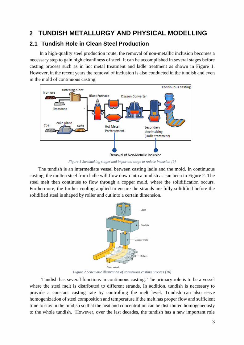
In a high-quality steel production route, the removal of non-metallic inclusion becomes a
necessary step to gain high cleanliness of steel. It can be accomplished in several stages before
casting process such as in hot metal treatment and ladle treatment as shown in Figure 1.
However, in the recent years the removal of inclusion is also conducted in the tundish and even
in the mold of continuous casting.
Figure 1 Steelmaking stages and important stage to reduce inclusion [9]
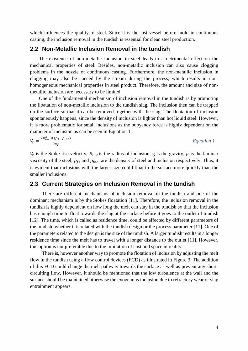
The tundish is an intermediate vessel between casting ladle and the mold. In continuous
casting, the molten steel from ladle will flow down into a tundish as can been in Figure 2. The
steel melt then continues to flow through a copper mold, where the solidification occurs.
Furthermore, the further cooling applied to ensure the strands are fully solidified before the
solidified steel is shaped by roller and cut into a certain dimension.
Figure 2 Schematic illustration of continuous casting process [10]
Tundish has several functions in continuous casting. The primary role is to be a vessel
where the steel melt is distributed to different strands. In addition, tundish is necessary to
provide a constant casting rate by controlling the melt level. Tundish can also serve
homogenization of steel composition and temperature if the melt has proper flow and sufficient
time to stay in the tundish so that the heat and concentration can be distributed homogeneously
to the whole tundish. However, over the last decades, the tundish has a new important role
4
which influences the quality of steel. Since it is the last vessel before mold in continuous
casting, the inclusion removal in the tundish is essential for clean steel production.
2.2 Non-Metallic Inclusion Removal in the tundish
The existence of non-metallic inclusion in steel leads to a detrimental effect on the
mechanical properties of steel. Besides, non-metallic inclusion can also cause clogging
problems in the nozzle of continuous casting. Furthermore, the non-metallic inclusion in
clogging may also be carried by the stream during the process, which results in non-
homogeneous mechanical properties in steel product. Therefore, the amount and size of non-
metallic inclusion are necessary to be limited.
One of the fundamental mechanism of inclusion removal in the tundish is by promoting
the floatation of non-metallic inclusion to the tundish slag. The inclusion then can be trapped
on the surface so that it can be removed together with the slag. The floatation of inclusion
spontaneously happens, since the density of inclusion is lighter than hot liquid steel. However,
it is more problematic for small inclusions as the buoyancy force is highly dependent on the
diameter of inclusion as can be seen in Equation 1.
𝑉𝑟 =2𝑅𝑖𝑛𝑐
2 𝑔 (𝜌𝑓−𝜌𝑖𝑛𝑐)
9𝜇𝑓 Equation 11
𝑉𝑟 is the Stoke rise velocity, 𝑅𝑖𝑛𝑐 is the radius of inclusion, g is the gravity, 𝜇 is the laminar
viscosity of the steel, 𝜌𝑓, and 𝜌𝑖𝑛𝑐 are the density of steel and inclusion respectively. Thus, it
is evident that inclusions with the larger size could float to the surface more quickly than the
smaller inclusions.
2.3 Current Strategies on Inclusion Removal in the tundish
There are different mechanisms of inclusion removal in the tundish and one of the
dominant mechanism is by the Stokes floatation [11]. Therefore, the inclusion removal in the
tundish is highly dependent on how long the melt can stay in the tundish so that the inclusion
has enough time to float towards the slag at the surface before it goes to the outlet of tundish
[12]. The time, which is called as residence time, could be affected by different parameters of
the tundish, whether it is related with the tundish design or the process parameter [11]. One of
the parameters related to the design is the size of the tundish. A larger tundish results in a longer
residence time since the melt has to travel with a longer distance to the outlet [11]. However,
this option is not preferable due to the limitation of cost and space in reality.
There is, however another way to promote the flotation of inclusion by adjusting the melt
flow in the tundish using a flow control devices (FCD) as illustrated in Figure 3. The addition
of this FCD could change the melt pathway towards the surface as well as prevent any short-
circuiting flow. However, it should be mentioned that the low turbulence at the wall and the
surface should be maintained otherwise the exogenous inclusion due to refractory wear or slag
entrainment appears.

5
Figure 3 Different type of flow control devices (FCD) in the tundish [13]
Nevertheless, the addition of FCD is limited by the available space inside the tundish.
In addition, it is also highly dependent on tundish design. The parameter, such as the location
or the height of turbo-stopper, influences the mixing phenomena significantly [8]. The different
design of baffles can also create different phenomena which are very specific for every tundish
[5, 7]. Moreover, the position of strand and casting parameter such as shroud immersion depth
can also affect the performance of FCD [2, 8]. Therefore the consideration when selecting a
type and design of FCD must involve both tundish and casting parameters. Another
disadvantage is the FCD is susceptible to wear for long time usage. This can affect the
productivity, quality and as well as the total cost of its implementation. The last, the FCD
cannot provide the adjustment of flow for the whole process time.
The other method to adjust the melt flow inside tundish is by performing a stirring by
argon gas or electromagnetic stirring (EMS). Theoretically, the stirring enhances the
probability of collision and agglomeration between inclusions resulting in a larger size and
floatation velocity [11]. In addition, it also helps the temperature and composition
homogenization due to increasing of mixing intensity. However, the gas stirring is limited by
injection rate due to a possibility of slag entrainment may occur. The limitation of using FCD
and argon stirring could be partly solved by using EMS, which is investigated in this project.
2.4 Tundish Flow
The main objective when designing a tundish is to provide a melt flow that promotes
floatation of inclusions and a homogeneous composition in the whole tundish [14]. On the other
hand, the flow should be carefully controlled to prevent over-stirring that may induce an
exogenous inclusion in the melt. In this chapter, the model of flow characteristic in the tundish
was discussed and the preferable flow was also elaborated.
2.4.1 Tundish Flow Characterization
Since the melt flow affects the performance of tundish, a Combined Models of flow
characterization has been developed by Sahai and Emi [11]. In this model, the flow inside
tundish consists of three types: Plug flow, well-mixed, and dead volumes.
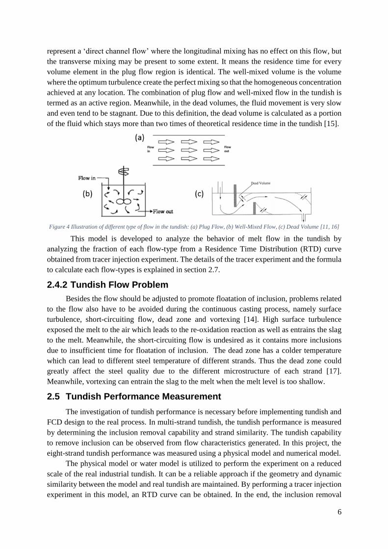
Figure 4 illustrates the difference between those flows in the tundish. The plug volumes
6
represent a ‘direct channel flow’ where the longitudinal mixing has no effect on this flow, but
the transverse mixing may be present to some extent. It means the residence time for every
volume element in the plug flow region is identical. The well-mixed volume is the volume
where the optimum turbulence create the perfect mixing so that the homogeneous concentration
achieved at any location. The combination of plug flow and well-mixed flow in the tundish is
termed as an active region. Meanwhile, in the dead volumes, the fluid movement is very slow
and even tend to be stagnant. Due to this definition, the dead volume is calculated as a portion
of the fluid which stays more than two times of theoretical residence time in the tundish [15].
Figure 4 Illustration of different type of flow in the tundish: (a) Plug Flow, (b) Well-Mixed Flow, (c) Dead Volume [11, 16]
This model is developed to analyze the behavior of melt flow in the tundish by
analyzing the fraction of each flow-type from a Residence Time Distribution (RTD) curve
obtained from tracer injection experiment. The details of the tracer experiment and the formula
to calculate each flow-types is explained in section 2.7.
2.4.2 Tundish Flow Problem
Besides the flow should be adjusted to promote floatation of inclusion, problems related
to the flow also have to be avoided during the continuous casting process, namely surface
turbulence, short-circuiting flow, dead zone and vortexing [14]. High surface turbulence
exposed the melt to the air which leads to the re-oxidation reaction as well as entrains the slag
to the melt. Meanwhile, the short-circuiting flow is undesired as it contains more inclusions
due to insufficient time for floatation of inclusion. The dead zone has a colder temperature
which can lead to different steel temperature of different strands. Thus the dead zone could
greatly affect the steel quality due to the different microstructure of each strand [17].
Meanwhile, vortexing can entrain the slag to the melt when the melt level is too shallow.
2.5 Tundish Performance Measurement
The investigation of tundish performance is necessary before implementing tundish and
FCD design to the real process. In multi-strand tundish, the tundish performance is measured
by determining the inclusion removal capability and strand similarity. The tundish capability
to remove inclusion can be observed from flow characteristics generated. In this project, the
eight-strand tundish performance was measured using a physical model and numerical model.
The physical model or water model is utilized to perform the experiment on a reduced
scale of the real industrial tundish. It can be a reliable approach if the geometry and dynamic
similarity between the model and real tundish are maintained. By performing a tracer injection
experiment in this model, an RTD curve can be obtained. In the end, the inclusion removal
7
capability can be determined by calculating the fraction of flow-type from the RTD curve.
Meanwhile, the numerical model is carried out by simulating the fluid flow in CFD
software. Besides analyzing the RTD Curve, the numerical model is also useful to predict the
behavior of melt flow in the tundish. The relevant variables in fluid flow such as turbulence
energy in any location of tundish can also be observed. Another advantage is the quick result
may be obtained for every configuration change in the tundish. However, the appropriate
assumption and correct input of boundary condition is necessary to obtain a reliable result.
For both methods, following variables are determined in order to quantify the
performance of tundish as a metallurgical reactor to remove inclusions:
1. Minimum dead volume;
2. High Mixing Volume;
3. The melt flow with less turbulence near the wall and slag-metal interface;
4. High Plug Volume or no short-circuiting melt flow from inlet to the outlet of
tundish;
5. The Long residence time of melt in the tundish;
6. Large Plug to dead or mixing ratio [11].
2.6 Residence Time Distribution Experiment
The residence time distribution (RTD) curve has been obtained by performing the
experiment in water model. A certain amount of soluble and non-reactive chemical is injected
through the inlet so that the tracer flows together with the water stream. The tracer should be
detectable so that the important phenomena such as short-circuiting stream could be easily
observed. Commonly, the tracer used in such experiment is a dye, acid or salt. The time in
which the tracer injected is defined as t =0 and then the concentration of tracer will be measured
at the outlet of the model. The results are plotted as an RTD curve where the dimensionless
time and the dimensionless concentration becomes x- and y-axes respectively.
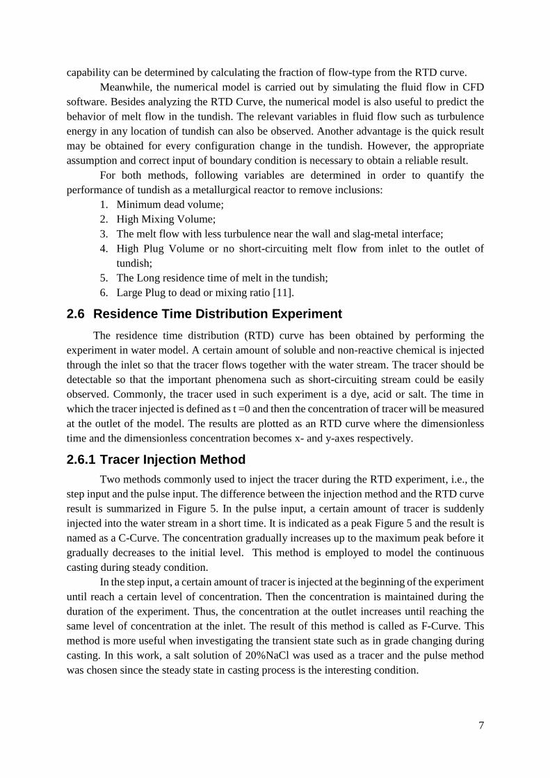
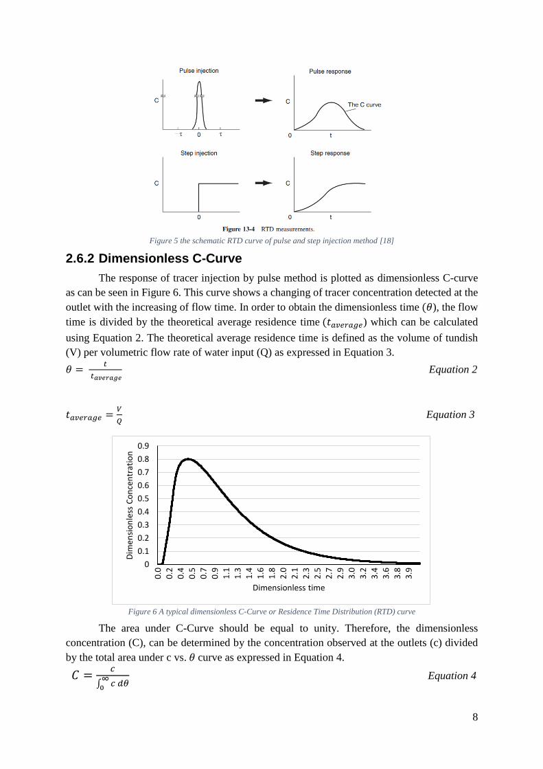
2.6.1 Tracer Injection Method
Two methods commonly used to inject the tracer during the RTD experiment, i.e., the
step input and the pulse input. The difference between the injection method and the RTD curve
result is summarized in Figure 5. In the pulse input, a certain amount of tracer is suddenly
injected into the water stream in a short time. It is indicated as a peak Figure 5 and the result is
named as a C-Curve. The concentration gradually increases up to the maximum peak before it
gradually decreases to the initial level. This method is employed to model the continuous
casting during steady condition.
In the step input, a certain amount of tracer is injected at the beginning of the experiment
until reach a certain level of concentration. Then the concentration is maintained during the
duration of the experiment. Thus, the concentration at the outlet increases until reaching the
same level of concentration at the inlet. The result of this method is called as F-Curve. This
method is more useful when investigating the transient state such as in grade changing during
casting. In this work, a salt solution of 20%NaCl was used as a tracer and the pulse method
was chosen since the steady state in casting process is the interesting condition.
8
Figure 5 the schematic RTD curve of pulse and step injection method [18]
2.6.2 Dimensionless C-Curve
The response of tracer injection by pulse method is plotted as dimensionless C-curve
as can be seen in Figure 6. This curve shows a changing of tracer concentration detected at the
outlet with the increasing of flow time. In order to obtain the dimensionless time (𝜃), the flow
time is divided by the theoretical average residence time (𝑡𝑎𝑣𝑒𝑟𝑎𝑔𝑒) which can be calculated
using Equation 2. The theoretical average residence time is defined as the volume of tundish
(V) per volumetric flow rate of water input (Q) as expressed in Equation 3.
𝜃 = 𝑡
𝑡𝑎𝑣𝑒𝑟𝑎𝑔𝑒 Equation 2
𝑡𝑎𝑣𝑒𝑟𝑎𝑔𝑒 =𝑉
𝑄 Equation 3
Figure 6 A typical dimensionless C-Curve or Residence Time Distribution (RTD) curve
The area under C-Curve should be equal to unity. Therefore, the dimensionless
concentration (C), can be determined by the concentration observed at the outlets (c) divided
by the total area under c vs. 𝜃 curve as expressed in Equation 4.
𝐶 =𝑐
∫ 𝑐 𝑑𝜃∞
0
Equation 4
0
0.1
0.2
0.3
0.4
0.5
0.6
0.7
0.8
0.9
0.0
0.2
0.4
0.5
0.7
0.9
1.1
1.3
1.4
1.6
1.8
2.0
2.1
2.3
2.5
2.7
2.9
3.0
3.2
3.4
3.6
3.8
3.9
Dim
ensi
on
less
Co
nce
ntr
atio
n
Dimensionless time

9
When investigating the similarity between strands, the mean of dimensionless residence
time (𝜃𝑚) is necessary to describe the difference of RTD curve and to calculate the dead volume
fraction. The mean residence time can be determined by Equation 5.
𝜃𝑚 =∑ 𝜃𝑖𝑐𝑖 ∞
𝑖=0
∑ 𝑐𝑖 ∞𝑖=0
Equation 5
2.7 Flow Characterization Calculation
The dimensionless C-Curve was used to study the similarity between strands in the model
as well as the tundish performance by determining the flow characteristics. The explanation of
each flow characteristics and its formula is explained in this section.
2.7.1 RTD curve of Plug flow
Due to the absence of longitudinal mixing in the ideal plug flow, the liquid melt will
have the same residence time in the tundish. This will produce a maximum peak at the
theoretical residence time (𝜃 = 1 ) as shown in Figure 7. However, in the actual process, a
horizontal mixing always presence due to the turbulence or the molecular diffusion [11]. This
lead to a dispersed plug flow which has a broader peak than the ideal condition as illustrated in
Figure 8.
Figure 7 RTD curve of ideal plug flow
Figure 8 RTD curves of Non-ideal plug flow with various dispersion number constants [16]
0.00
0.20
0.40
0.60
0.80
1.00
1.20
0.0
0.1
0.2
0.3
0.4
0.5
0.6
0.7
0.7
0.8
0.9
1.0
1.1
1.2
1.3
1.4
1.5
1.6
1.7
1.8
1.9
Dim
ensi
on
less
Co
nce
ntr
atio
n
Dimensionless time

10
2.7.2 RTD curve of Well-Mixed Volume
In an ideal well-mixed flow, the extreme mixing causes an identical tracer concentration
at the outlet and at any position in the tundish. The residence curve of this flow is derived from
the mass balance equation of tracer injection as written in Equation 6 to Equation 9 [11].
𝑅𝑎𝑡𝑒 𝑜𝑓 𝑡𝑟𝑎𝑐𝑒𝑟 𝑖𝑛𝑝𝑢𝑡 − 𝑅𝑎𝑡𝑒 𝑜𝑓 𝑇𝑟𝑎𝑐𝑒 𝑂𝑢𝑡𝑝𝑢𝑡 = 𝑅𝑎𝑡𝑒 𝑜𝑓 𝑎𝑐𝑐𝑢𝑚𝑢𝑙𝑎𝑡𝑖𝑜𝑛 Equation 6
𝑄(0) − 𝑄(𝑐) = 𝑑
𝑑𝑡𝑉𝑐 Equation 7
𝑑𝑐
𝐶= −
𝑄
𝑉 𝑑𝑡 Equation 8
The integration of Equation 8 leads to the solution as stated in Equation 9. From this equation,
the RTD curve is plotted and presented in Figure 9.
𝑐 = 𝑒−𝜃 Equation 9
In an ideal mix curve, the dimensionless concentration at 𝜃 = 0 equals the average
concentration of tracer injected (𝐶 = 1). Then the concentration at any point of tundish
decreases exponentially with the increasing of time.
Figure 9 RTD curve of ideal mix volume
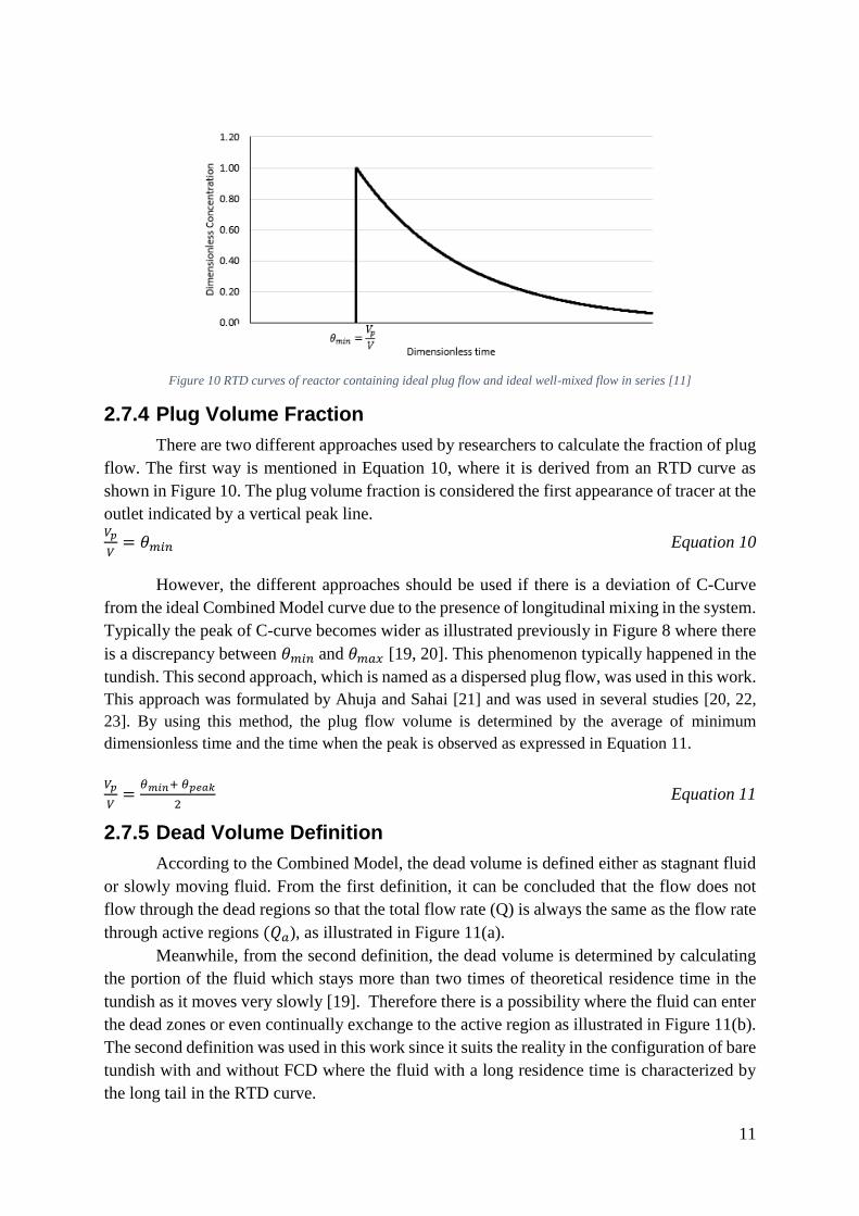
2.7.3 Combined Model
Sahai and Emi proposed a new model for analyzing flow in the tundish based on an
assumption that the tundish contains three different type of flow: plug flow volume, well-mix
flow volume and the dead volume [11]. The model is derived based on a configuration where
the plug flow and well-mixed flow presence in a series reactor. The result of RTD curve of this
configuration is presented in Figure 10. In this model, the minimum residence time is
considered as the plug volume fraction. Meanwhile, the dead zone is defined as a melt that
moves very slowly or tends to be stagnant so that it has a long residence time in the tundish.
The further explanation regarding the calculation of those three flow-type fractions are
discussed in the next chapter.
0.00
0.20
0.40
0.60
0.80
1.00
1.20
0.0
0.2
0.3
0.5
0.6
0.8
0.9
1.1
1.3
1.4
1.6
1.7
1.9
2.0
2.2
2.4
2.5
2.7
2.8
3.0
3.1
3.3
3.5
3.6
Dim
ensi
on
less
Co
nce
ntr
atio
n
Dimensionless time
11
Figure 10 RTD curves of reactor containing ideal plug flow and ideal well-mixed flow in series [11]
2.7.4 Plug Volume Fraction
There are two different approaches used by researchers to calculate the fraction of plug
flow. The first way is mentioned in Equation 10, where it is derived from an RTD curve as
shown in Figure 10. The plug volume fraction is considered the first appearance of tracer at the
outlet indicated by a vertical peak line. 𝑉𝑝
𝑉= 𝜃𝑚𝑖𝑛 Equation 10
However, the different approaches should be used if there is a deviation of C-Curve
from the ideal Combined Model curve due to the presence of longitudinal mixing in the system.
Typically the peak of C-curve becomes wider as illustrated previously in Figure 8 where there
is a discrepancy between 𝜃𝑚𝑖𝑛 and 𝜃𝑚𝑎𝑥 [19, 20]. This phenomenon typically happened in the
tundish. This second approach, which is named as a dispersed plug flow, was used in this work.
This approach was formulated by Ahuja and Sahai [21] and was used in several studies [20, 22,
23]. By using this method, the plug flow volume is determined by the average of minimum
dimensionless time and the time when the peak is observed as expressed in Equation 11.
𝑉𝑝
𝑉=
𝜃𝑚𝑖𝑛+ 𝜃𝑝𝑒𝑎𝑘
2 Equation 11
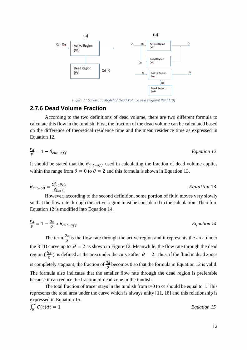
2.7.5 Dead Volume Definition
According to the Combined Model, the dead volume is defined either as stagnant fluid
or slowly moving fluid. From the first definition, it can be concluded that the flow does not
flow through the dead regions so that the total flow rate (Q) is always the same as the flow rate
through active regions (𝑄𝑎), as illustrated in Figure 11(a).
Meanwhile, from the second definition, the dead volume is determined by calculating
the portion of the fluid which stays more than two times of theoretical residence time in the
tundish as it moves very slowly [19]. Therefore there is a possibility where the fluid can enter
the dead zones or even continually exchange to the active region as illustrated in Figure 11(b).
The second definition was used in this work since it suits the reality in the configuration of bare
tundish with and without FCD where the fluid with a long residence time is characterized by
the long tail in the RTD curve.
12
Figure 11 Schematic Model of Dead Volume as a stagnant fluid [19]
2.7.6 Dead Volume Fraction
According to the two definitions of dead volume, there are two different formula to
calculate this flow in the tundish. First, the fraction of the dead volume can be calculated based
on the difference of theoretical residence time and the mean residence time as expressed in
Equation 12.
𝑉𝑑
𝑉= 1 − 𝜃𝑐𝑢𝑡−𝑜𝑓𝑓 Equation 12
It should be stated that the 𝜃𝑐𝑢𝑡−𝑜𝑓𝑓 used in calculating the fraction of dead volume applies
within the range from 𝜃 = 0 to 𝜃 = 2 and this formula is shown in Equation 13.
𝜃cut−off =∑ 𝜃𝑖
2𝑖=0 𝑐𝑖
∑ 𝑐𝑖2𝑖=0
𝐸𝑞𝑢𝑎𝑡𝑖𝑜𝑛 13
However, according to the second definition, some portion of fluid moves very slowly
so that the flow rate through the active region must be considered in the calculation. Therefore
Equation 12 is modified into Equation 14.
𝑉𝑑
𝑉= 1 −
𝑄𝑎
𝑄 𝑥 𝜃𝑐𝑢𝑡−𝑜𝑓𝑓 Equation 14
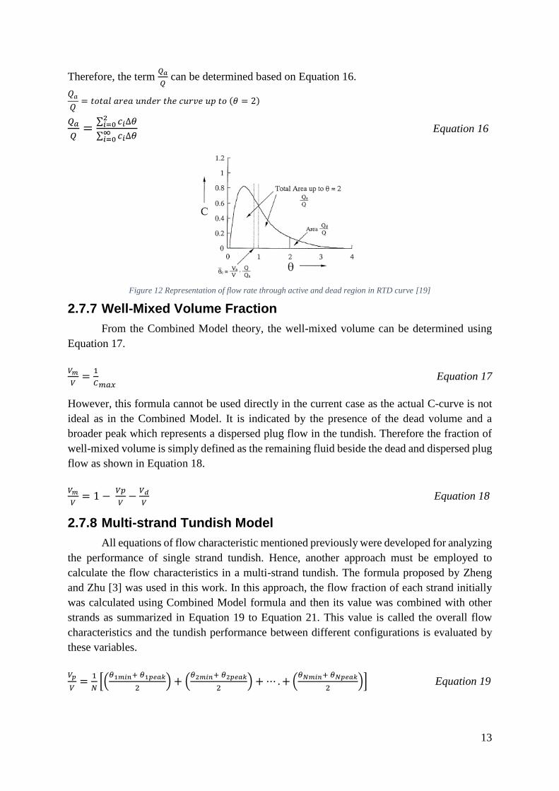
The term 𝑄𝑎
𝑄 is the flow rate through the active region and it represents the area under
the RTD curve up to 𝜃 = 2 as shown in Figure 12. Meanwhile, the flow rate through the dead
region ( 𝑄𝑑
𝑄 ) is defined as the area under the curve after 𝜃 = 2. Thus, if the fluid in dead zones
is completely stagnant, the fraction of 𝑄𝑑
𝑄 becomes 0 so that the formula in Equation 12 is valid.
The formula also indicates that the smaller flow rate through the dead region is preferable
because it can reduce the fraction of dead zone in the tundish.
The total fraction of tracer stays in the tundish from t=0 to ∞ should be equal to 1. This
represents the total area under the curve which is always unity [11, 18] and this relationship is
expressed in Equation 15.
∫ 𝐶(𝑡)𝑑𝑡∞
0= 1 Equation 15
13
Therefore, the term 𝑄𝑎
𝑄 can be determined based on Equation 16.
𝑄𝑎
𝑄= 𝑡𝑜𝑡𝑎𝑙 𝑎𝑟𝑒𝑎 𝑢𝑛𝑑𝑒𝑟 𝑡ℎ𝑒 𝑐𝑢𝑟𝑣𝑒 𝑢𝑝 𝑡𝑜 (𝜃 = 2)
𝑄𝑎
𝑄=
∑ 𝑐𝑖∆𝜃2𝑖=0
∑ 𝑐𝑖∆𝜃∞𝑖=0
Equation 16
Figure 12 Representation of flow rate through active and dead region in RTD curve [19]
2.7.7 Well-Mixed Volume Fraction
From the Combined Model theory, the well-mixed volume can be determined using
Equation 17.
𝑉𝑚
𝑉=
1
𝐶𝑚𝑎𝑥 Equation 17
However, this formula cannot be used directly in the current case as the actual C-curve is not
ideal as in the Combined Model. It is indicated by the presence of the dead volume and a
broader peak which represents a dispersed plug flow in the tundish. Therefore the fraction of
well-mixed volume is simply defined as the remaining fluid beside the dead and dispersed plug
flow as shown in Equation 18.
𝑉𝑚
𝑉= 1 −
𝑉𝑝
𝑉−
𝑉𝑑
𝑉 Equation 18
2.7.8 Multi-strand Tundish Model
All equations of flow characteristic mentioned previously were developed for analyzing
the performance of single strand tundish. Hence, another approach must be employed to
calculate the flow characteristics in a multi-strand tundish. The formula proposed by Zheng
and Zhu [3] was used in this work. In this approach, the flow fraction of each strand initially
was calculated using Combined Model formula and then its value was combined with other
strands as summarized in Equation 19 to Equation 21. This value is called the overall flow
characteristics and the tundish performance between different configurations is evaluated by
these variables.
𝑉𝑝
𝑉=
1
𝑁[(
𝜃1𝑚𝑖𝑛+ 𝜃1𝑝𝑒𝑎𝑘
2) + (
𝜃2𝑚𝑖𝑛+ 𝜃2𝑝𝑒𝑎𝑘
2) + ⋯ . + (
𝜃𝑁𝑚𝑖𝑛+ 𝜃𝑁𝑝𝑒𝑎𝑘
2)] Equation 19

14
𝑉𝑑
𝑉= 1 −
1
𝑁(
𝑄1𝑎
𝑄1 𝑥 𝜃1𝑐𝑢𝑡−𝑜𝑓𝑓 +
𝑄2𝑎
𝑄2 𝑥 𝜃2𝑐𝑢𝑡−𝑜𝑓𝑓 + ⋯ +
𝑄𝑁𝑎
𝑄𝑁 𝑥 𝜃𝑁𝑐𝑢𝑡−𝑜𝑓𝑓 ) Equation 20
𝑉𝑚
𝑉= 1 −
𝑉𝑝
𝑉−
𝑉𝑑
𝑉 Equation 21
2.7.9 Strand Similarity
Besides the flow characteristics which become a reference to measure tundish
capability to remove inclusion, a similarity among strands also become an essential parameter
to measure the performance of multi-strands tundish. It is because the excellent similarity
among strands is essential to guarantee an uniform temperature and steel cleanliness.
Unfortunately, researchers have a different way to measure this parameter, such as by
comparing the maximum concentration of the inner and outer strand tundish [24] or by
calculating the standard deviation of some important variables, i.e., the first time tracer appears
at the outlets [25, 26]. However, an approach developed by Zheng and Zhu was used in this
work and the formula is presented by Equation 22 [5]. The N in the equation represents the
number of strands, z is the number of instantaneous time 𝑡𝑗 and ��(𝑡𝑗) is the average of
dimensionless concentration at time 𝑡𝑗.
𝑆𝑁 =
1
𝑍∑ {
[∑ (𝐶𝑖(𝑡𝑗)−��(𝑡𝑗))2𝑁𝑗=1 ]
𝑁−1}
1/2
𝑍𝑗=1 Equation 22
In the other word, 𝑆𝑁 is the strand similarity from strand 1 to N which defined as the
average of total standard deviation of the dimensionless concentration from time j=1 to t=z.
Therefore, the lower this value means the deviation of concentration in all strands at every time
is small so that it leads to the better strand similarity. This approach is better than others since
it considers all of the concentration of every strand in every recorded time in the experiment
[5].
2.8 Tundish Water Model Criteria
The utilization of water model to perform RTD experiment is useful due to its reliability
to represent the actual industrial tundish. However, it is obvious that several parameters are
different and it is impossible to create similar condition as the reality. Hence, the model has to
fulfill a number of similarity criteria, i.e., geometric, dynamic, kinetic, thermal, and chemical
similarity. Since the steel melt is assumed as non-reactive in isothermal condition, the thermal
and chemical similarity consideration is excluded in this study.
2.8.1 Geometric Similarity
The tundish size has a great effect on the capability of tundish to remove inclusions
since the melt can stay longer in a bigger tundish [1]. Besides, the design parameter such as
FCD location in the tundish also influences the tundish performance [27]. Thus, the changing
of geometry may lead to a different result in the physical modelling. In order to minimize this
effect, each linear dimensions in the tundish have to be reduced by the same scale factor 𝜆 as
shown in Equation 23. Lm is the dimension of model and Lp is the prototype or real industrial

15
tundish dimension, so that λ may vary from 0 to 1. A reduced scale model has a benefit
concerning space and for experiment setting. Nevertheless, a reduced scale model has the
drawback as it is impossible to achieve a similar Froude and Reynold number in dynamic
similarity consideration [15]. The more detail explanation of the problem to achieve a similar
Froude and Reynold Number in dynamic similarity is explained in section 2.8.2.
𝜆 =𝐿𝑚
𝐿𝑝 Equation 23
2.8.2 Dynamic Similarity Consideration
The dynamic similarity between industrial tundish and water model entails that the
presence of all forces act on steel melt must be changed by a certain scale in the water model.
In the tundish, the considered forces are the forces related to fluid flow behavior such as the
gravity, the viscosity and the inertial forces. In fluid mechanics, the flow behavior could be
expressed in the form of a ratio between the two forces which is known as the Reynold and
Froude number. The Reynold number is a ratio between the inertial to the viscous forces
whereas the Froude number represents the ratio of viscous to the gravitational forces. Formulas
of those two similarity considerations were shown in Equation 24 and Equation 25 where the
Re and Fr is the symbol of Reynold and Froude number respectively, 𝜐 is the velocity of the
fluid, 𝜌 is the density of the fluid, 𝐿 is the characteristic length and 𝜇 is the dynamic viscosity
of the melt.
𝑅𝑒 =𝜐𝜌𝐿
𝜇 Equation 24
𝐹𝑟 =𝜐2
𝑔𝐿 Equation 25
In dynamic similarity consideration, the Reynold and Froude numbers are desired to be
similar between model and the industrial tundish. For Reynold number similarity, this leads to
Equation 26.
(𝜐𝜌𝐿
𝜇)
𝑚𝑜𝑑𝑒𝑙= (
𝜐𝜌𝐿
𝜇)
𝑖𝑛𝑑𝑢𝑠𝑡𝑟𝑖𝑎𝑙 𝑡𝑢𝑛𝑑𝑖𝑠ℎ Equation 26
Since the difference between the kinematic viscosity of steel at 1600℃ and water at room
temperature as shown in Table 1 is insignificant, the Equation 26 can be simplified into
Equation 27. By using a similar step in Froude number similarity consideration, the relationship
between model and industrial tundish is expressed in Equation 28. Table 1 Comparison of kinematic viscosity of steel and water [28]
𝜐𝑚𝑜𝑑𝑒𝑙 ≈1
𝜆 𝜐𝑖𝑛𝑑𝑢𝑠𝑡𝑟𝑖𝑎𝑙 𝑡𝑢𝑛𝑑𝑖𝑠ℎ Equation 27
𝜐𝑚𝑜𝑑𝑒𝑙 ≈ √𝜆 𝜐𝑖𝑛𝑑𝑢𝑠𝑡𝑟𝑖𝑎𝑙 𝑡𝑢𝑛𝑑𝑖𝑠ℎ Equation 28
Based on Equation 27 and Equation 28, it is clear that the similarity of Froude and
Reynold number can only be achieved in a full-scale model as 𝜆 = 1. It is impossible to satisfy
Property Steel at 1600 ℃ Water at 20 ℃
Dynamic Viscosity, 𝜇 (kg m-1 s-1) 0.0064 0.001
Density,𝜌 (kg m-3) 7014 1000
Kinematic Viscosity, 𝜇
𝜌 (m2 s-1) 1. 10-6 0.913. 10-6
16
both number in a reduced scale model, because when the Reynold number similarity is
achieved, the velocity becomes higher in the model and the opposite result occurs if the Froude
number similarity becomes the reference. That is the reason why researchers have a different
opinion regarding which number should be used when developing a water model.
In relation with this problem, a comparison study of the importance of Reynold and
Froude number on fluid flow behavior in the tundish has been carried out by Sahai and Emi.
They stated that actually neither of the Reynold number nor Froude number similarity is
necessary to predict the fluid flow behavior in water model experiment. However, the Froude
number similarity is useful for the prediction of the inclusion removal in the tundish [15].
The reason of why Reynold number similarity is not important in water model
experiment is because the turbulent flow becomes the dominant fluid flow in the tundish. In
turbulent flow, a combination of molecular and turbulent viscosity is used to describe the
diffusive momentum transfer capability. The turbulent viscosity is much important due to the
exchange happened by eddies length are much dominant than by the molecular exchange.
Therefore, a Reynold number similarity is not so important to be fulfilled as in turbulent flow
the inertia flow is much higher than the viscous forces. The Reynold number similarity is only
important to be considered in a laminar flow where the viscous layer becomes the only
mechanism of diffusive momentum transfer [15].
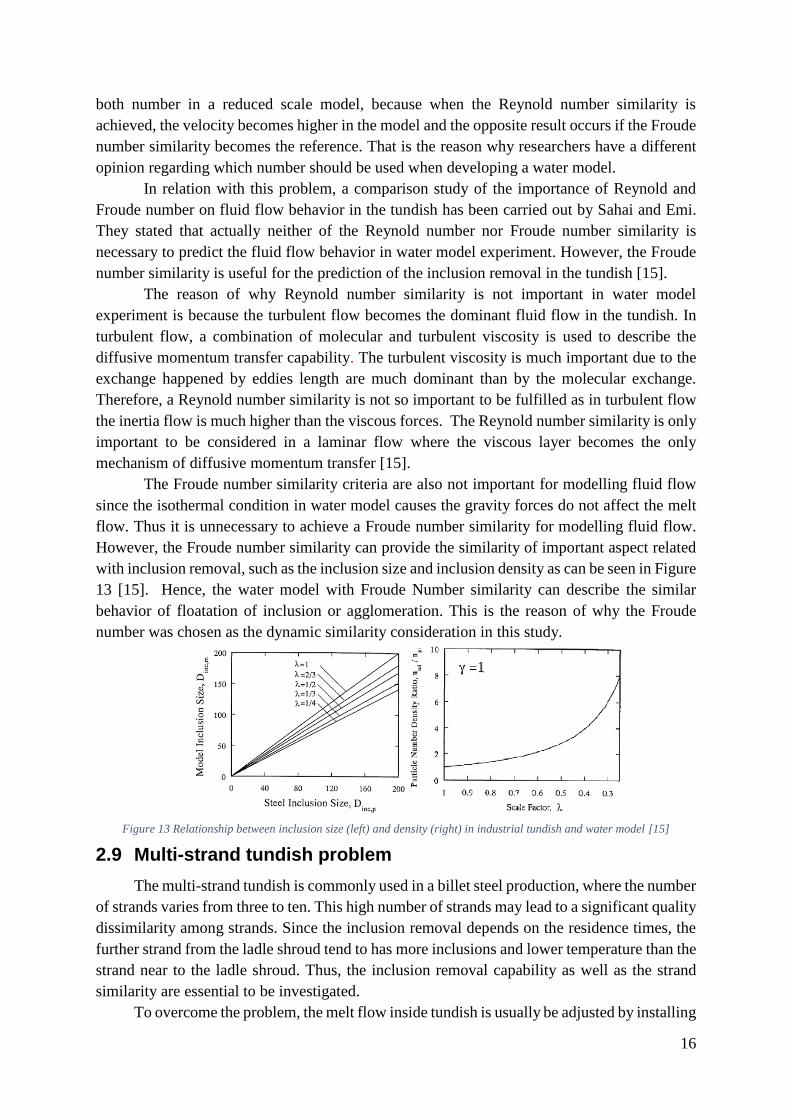
The Froude number similarity criteria are also not important for modelling fluid flow
since the isothermal condition in water model causes the gravity forces do not affect the melt
flow. Thus it is unnecessary to achieve a Froude number similarity for modelling fluid flow.
However, the Froude number similarity can provide the similarity of important aspect related
with inclusion removal, such as the inclusion size and inclusion density as can be seen in Figure
13 [15]. Hence, the water model with Froude Number similarity can describe the similar
behavior of floatation of inclusion or agglomeration. This is the reason of why the Froude
number was chosen as the dynamic similarity consideration in this study.
Figure 13 Relationship between inclusion size (left) and density (right) in industrial tundish and water model [15]
2.9 Multi-strand tundish problem
The multi-strand tundish is commonly used in a billet steel production, where the number
of strands varies from three to ten. This high number of strands may lead to a significant quality
dissimilarity among strands. Since the inclusion removal depends on the residence times, the
further strand from the ladle shroud tend to has more inclusions and lower temperature than the
strand near to the ladle shroud. Thus, the inclusion removal capability as well as the strand
similarity are essential to be investigated.
To overcome the problem, the melt flow inside tundish is usually be adjusted by installing

17
several flow control devices (FCD) such as dams, weirds, or baffle wall. However, the proper
FCD varies for different tundish geometry and design. This means the solution of optimum
FCD design and its position in the tundish is very specific for each case. In addition, the multi-
strand tundish typically has a limited working space and the refractory material may
contaminate the steel. Another weakness of FCD is it is vulnerable to wear for long-term usage.
It affects the productivity, quality and also the total cost of its implementation. The last, the
FCD cannot provide the adjustment of melt flow for the whole process time.
One solution that could overcome those problems is using electromagnetic stirring
(EMS) for stirring the melt. This technology has been developed by ABB Metallurgy in
Västerås, Sweden. The horizontal stirring created by EMS will mix and adjust the melt flow
then it homogenize the composition and temperature. Thus, there is a possibility to replace
FCD with EMS. In addition, EMS is also more flexible to be controlled based on the tundish
design and the casting process. Despite being more expensive than FCD, EMS has a much
longer lifetime that the total cost becomes comparable. However, the comprehensive behavior
of the flow generated by EMS has not been understood due to the lack of studies related with
EMS in the tundish.
2.10 Electromagnetic Stirring Technology
EMS is a set of tools which can provide mixing in the melt with the help of
electromagnetic force generated by coil induction. This technology can be used as a method to
adjust flow behavior inside the tundish so that better steel cleanliness can be obtained. The
EMS unit consists of four components namely an electromagnetic coil, frequency converter,
transformer and a water station as can be seen in Figure 14.
Figure 14 Typical Electromagnetic Stirring System and Components [29]
The basic principle is the current from the converter will flow into the coil. This current
then will produce a strengthened electromagnetic field which penetrates into the steel melt.
Furthermore, the electromagnetic field induces a current in the steel melt. As a result, the
Lorentz Force will be generated in the steel melt and this becomes the source of stirring force.
Meanwhile, the water station act as a cooling unit for reducing the temperature of iron ore
inside the coil. In this work, the EMS will be replaced by the water pumps in the water model
experiment. This method has not been used previously in the tundish stirring. Even though it
is definitely not similar, however, it can be the good way to model the EMS in water.
18
3 BASIC THEORY OF NUMERICAL MODELLING
A Computational Fluid Dynamics (CFD) can be a method to predict the fluid behavior in
the tundish model by solving governing equations related to fluid flow. It can also complement
the result of physical experiments since it is allowed us to observe more variables related to
fluid flow. However, correct settings such as meshing or turbulence model are required in order
to have reliable results,. In this project, a CFD Software ANSYS Fluent 18.2 was used.
Theories behind some setup in this software are elaborated in this section.
3.1 Governing Equations
ANSYS Fluent simulates the fluid flow behavior based on the conservation of mass and
momentum equation. Since the tracer as a chemical species is injected during the water model
experiment, the conservation of species equation was activated. For simulating particle trap
during particle injection, a Discrete Phase Model (DPM) was selected. Meanwhile, the equation
of heat transfer was turned due to isothermal assumption. Those equations are solved together
during simulation in this work. Firstly, the mass and momentum are iterated until reach a steady
state condition. The conservation of species and discrete phase model equation are solved after
the tracer or inclusion particle injection in a transient simulation.
3.1.1 Conservation of Mass
The conservation of mass is expressed in Equation 29: 𝜕𝜌
𝜕𝑡+ 𝛻 ∙ 𝜌�� = 𝑆𝑚 Equation 29
The 𝐯 represents the fluid velocity, ρ is the density and Sm is the mass added to the system
from a dispersed phase, which equals to 0 in this work.
3.1.2 Conservation of Momentum
The equation of momentum conservation is expressed in Equation 30.
𝜕
𝜕𝑡(𝜌��) + 𝛻 ∙ (𝜌����) = −𝛻𝑝 + 𝜌�� + 𝛻 ∙ 𝜏 + �� Equation 30
This equation is derived from the Newton’s second law where p represents the static pressure,
g is the gravity and 𝜏 is the stress tensor acts on fluid and �� is the external force. The left side
in the equation is the initial force and the right side represents pressure forces, viscous forces
and external forces respectively. This equation, together with the mass continuity equation is
known as Navier-Stokes equation [30].
3.1.3 Species Transport Conservation
Fluent predicts the mass fraction changing of the species Yi, by solving the equation of
convection-diffusion of the solution as shown in Equation 31. 𝜕
𝜕𝑡(𝜌𝑌𝑖) + 𝛻 ∙ (𝜌��𝑌𝑖) = −𝛻 ∙ 𝐽𝑖
+ 𝑅𝑖 + 𝑆𝑖 Equation 31
𝑅𝑖 and 𝑆𝑖 represent the net rate of production of species i by chemical reaction and by addition
from any other sources respectively. Meanwhile, 𝑱𝒊 represents the diffusive flux which occurs

19
due to the difference between temperature and concentration in the system.
3.1.4 Discrete Phase Model (DPM)
The Discrete Phase Model (DPM) was used to study the particle trajectory from an
injection. In this work, the particle injected represents the alumina inclusion which is dispersed
due to turbulent flow. The particle trajectory is calculated by solving the particle force balance
equation as expressed in Equation 32.
𝑑𝑈𝑖𝑃
𝑑𝑡= 𝐹𝐷(𝑢𝑖 − 𝑢𝑖
𝑜) + 𝑔𝑖 (𝜌𝑝−𝜌
𝜌𝑝) +
𝐹𝑖
𝜌𝑝 Equation 32
The first part in the right side of Equation 32 represents the drag force, while the second and
the last are the gravity and external forces [31]. The DPM also consider the particle-wall
interactions such as escape, reflect or trap as shown in Figure 15.
Figure 15 Particle Interaction in DPM [31]
3.2 Turbulence Model
The turbulence flow is characterized by a high Reynold number, high degree of instability
as well as irregular movements where the mass, momentum and species transport is always
changing every time [32]. Because the flow inside tundish always involves the turbulence flow,
it needs to be modelled aiming to get more accurate results as in reality.
Figure 16 Turbulence flow structure [32]
There are small and large structures in a turbulence flow as shown in Figure 16. In order
to describe the behavior of turbulence in those structures, several mathematical models which
solves the energy and dissipation rate in those structures has been developed. In CFD, three
approaches can be used to solve the turbulence flow: Reynold Average Navier Stokes (RANS),
Large Eddy Simulation (LES) or Direct Numerical Simulation (DNS). The illustration of those
approaches is shown in Figure 17. The RANS method, specifically a Realizable 𝑘−∈ model
was chosen due to its simplicity.
3.2.1 The Reynold Average Navier Stokes (RANS) model
The basic principle of RANs model is expressed in Equation 34.
𝑈𝑖 = �� + 𝑈′ Equation 33
20
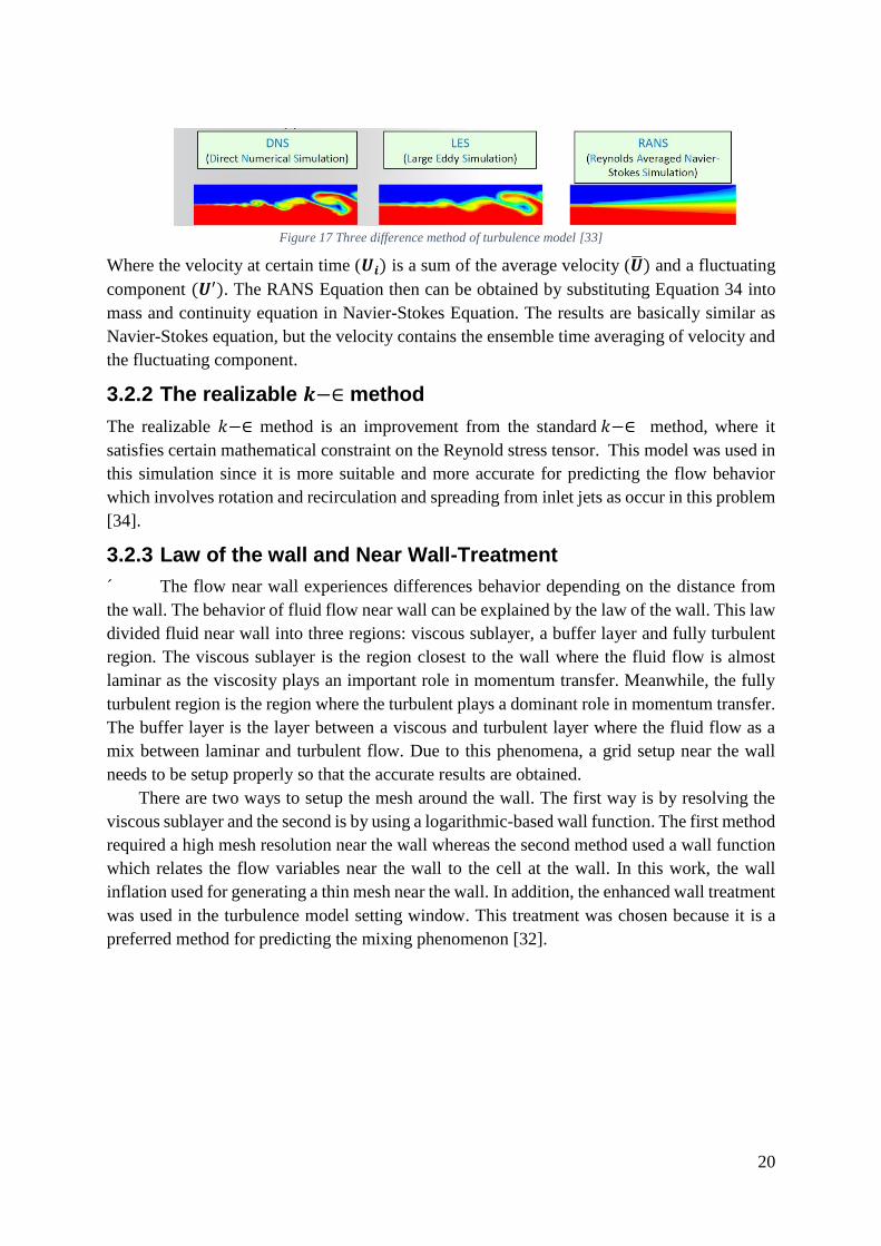
Figure 17 Three difference method of turbulence model [33]
Where the velocity at certain time (𝑼𝒊) is a sum of the average velocity (��) and a fluctuating
component (𝑼′). The RANS Equation then can be obtained by substituting Equation 34 into
mass and continuity equation in Navier-Stokes Equation. The results are basically similar as
Navier-Stokes equation, but the velocity contains the ensemble time averaging of velocity and
the fluctuating component.
3.2.2 The realizable 𝒌−∈ method
The realizable 𝑘−∈ method is an improvement from the standard 𝑘−∈ method, where it
satisfies certain mathematical constraint on the Reynold stress tensor. This model was used in
this simulation since it is more suitable and more accurate for predicting the flow behavior
which involves rotation and recirculation and spreading from inlet jets as occur in this problem
[34].
3.2.3 Law of the wall and Near Wall-Treatment
´ The flow near wall experiences differences behavior depending on the distance from
the wall. The behavior of fluid flow near wall can be explained by the law of the wall. This law
divided fluid near wall into three regions: viscous sublayer, a buffer layer and fully turbulent
region. The viscous sublayer is the region closest to the wall where the fluid flow is almost
laminar as the viscosity plays an important role in momentum transfer. Meanwhile, the fully
turbulent region is the region where the turbulent plays a dominant role in momentum transfer.
The buffer layer is the layer between a viscous and turbulent layer where the fluid flow as a
mix between laminar and turbulent flow. Due to this phenomena, a grid setup near the wall
needs to be setup properly so that the accurate results are obtained.
There are two ways to setup the mesh around the wall. The first way is by resolving the
viscous sublayer and the second is by using a logarithmic-based wall function. The first method
required a high mesh resolution near the wall whereas the second method used a wall function
which relates the flow variables near the wall to the cell at the wall. In this work, the wall
inflation used for generating a thin mesh near the wall. In addition, the enhanced wall treatment
was used in the turbulence model setting window. This treatment was chosen because it is a
preferred method for predicting the mixing phenomenon [32].
21
4 EXPERIMENT SETUP
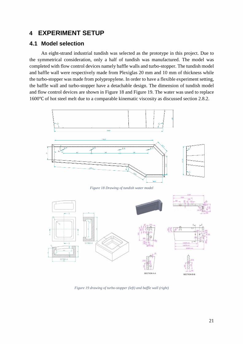
4.1 Model selection
An eight-strand industrial tundish was selected as the prototype in this project. Due to
the symmetrical consideration, only a half of tundish was manufactured. The model was
completed with flow control devices namely baffle walls and turbo-stopper. The tundish model
and baffle wall were respectively made from Plexiglas 20 mm and 10 mm of thickness while
the turbo-stopper was made from polypropylene. In order to have a flexible experiment setting,
the baffle wall and turbo-stopper have a detachable design. The dimension of tundish model
and flow control devices are shown in Figure 18 and Figure 19. The water was used to replace
1600℃ of hot steel melt due to a comparable kinematic viscosity as discussed section 2.8.2.
Figure 18 Drawing of tundish water model
Figure 19 drawing of turbo-stopper (left) and baffle wall (right)
22
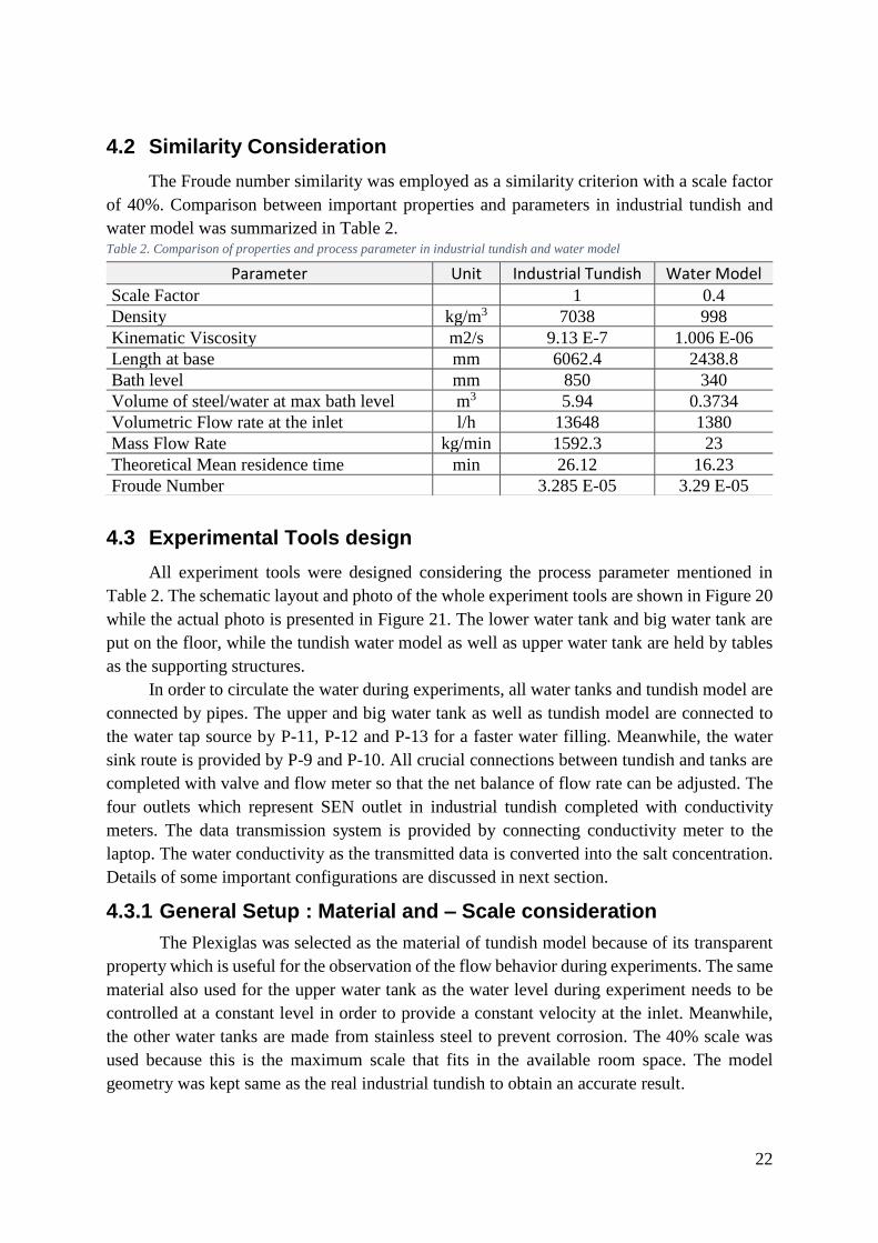
4.2 Similarity Consideration
The Froude number similarity was employed as a similarity criterion with a scale factor
of 40%. Comparison between important properties and parameters in industrial tundish and
water model was summarized in Table 2. Table 2. Comparison of properties and process parameter in industrial tundish and water model
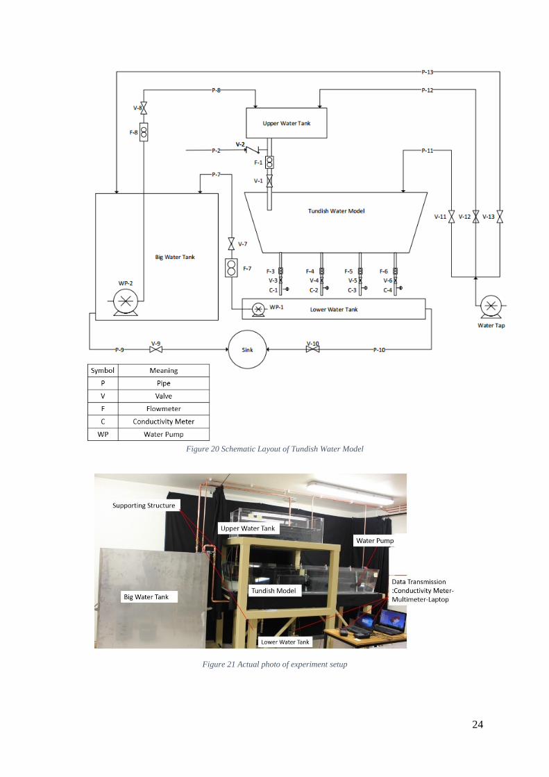
4.3 Experimental Tools design
All experiment tools were designed considering the process parameter mentioned in
Table 2. The schematic layout and photo of the whole experiment tools are shown in Figure 20
while the actual photo is presented in Figure 21. The lower water tank and big water tank are
put on the floor, while the tundish water model as well as upper water tank are held by tables
as the supporting structures.
In order to circulate the water during experiments, all water tanks and tundish model are
connected by pipes. The upper and big water tank as well as tundish model are connected to
the water tap source by P-11, P-12 and P-13 for a faster water filling. Meanwhile, the water
sink route is provided by P-9 and P-10. All crucial connections between tundish and tanks are
completed with valve and flow meter so that the net balance of flow rate can be adjusted. The
four outlets which represent SEN outlet in industrial tundish completed with conductivity
meters. The data transmission system is provided by connecting conductivity meter to the
laptop. The water conductivity as the transmitted data is converted into the salt concentration.
Details of some important configurations are discussed in next section.
4.3.1 General Setup : Material and – Scale consideration
The Plexiglas was selected as the material of tundish model because of its transparent
property which is useful for the observation of the flow behavior during experiments. The same
material also used for the upper water tank as the water level during experiment needs to be
controlled at a constant level in order to provide a constant velocity at the inlet. Meanwhile,
the other water tanks are made from stainless steel to prevent corrosion. The 40% scale was
used because this is the maximum scale that fits in the available room space. The model
geometry was kept same as the real industrial tundish to obtain an accurate result.
Parameter Unit Industrial Tundish Water Model Scale Factor 1 0.4
Density kg/m3 7038 998
Kinematic Viscosity m2/s 9.13 E-7 1.006 E-06
Length at base mm 6062.4 2438.8
Bath level mm 850 340
Volume of steel/water at max bath level m3 5.94 0.3734
Volumetric Flow rate at the inlet l/h 13648 1380
Mass Flow Rate kg/min 1592.3 23
Theoretical Mean residence time min 26.12 16.23
Froude Number 3.285 E-05 3.29 E-05

23
4.3.2 Water Tank Requirement
The three water tanks used in this work act as a temporary vessel as well as a water
storage for providing water during experiments. All tanks and water were filled by water and
the water is circulated from tundish model to the tanks until reach steady state as continuous
casting in the real process. Because of this, the total volume of all water tanks must be big
enough to supply the water up to four times of theoretical residence times with the desired flow
rate. The dimension of each water tank is listed in Table 3.
The smaller volume of upper and lower water tank compared to the big tank indicates
that the main role of these two tanks is not for providing water. The upper tank was built for
inlet installation and for providing tracer injection point location whereas the lower water tank
was fabricated to preserve the water from the four outlets. Table 3 Water tank dimension
4.3.3 Inlet and Outlet Configuration
The upper water tanks is a representation of a ladle in the industrial process whereas
the inlet acts a ladle shroud. In addition, the inlet is required since this is the location where the
tracer solution injected. The inlet was constructed from a 22 mm diameter of Plexiglas pipe
connected to the upper water tank as depicted in Figure 22. The inlet was completed with a
small pipe of 4 mm diameter for the tracer injection. The check valve was used as a connection
between the small pipe and the inlet so that the flow can only flow out to the inlet.
The outlets were fabricated from a small 12 mm diameter of Plexiglas pipe as displayed
in Figure 22. In this work, the outlet pipe furthest to the nearest from the inlet is called as strand
1 to strand 4. At the end of the outlets, a set of conductivity meter equipment was installed to
detect the changing of salt concentration during the experiment.
4.3.4 Turbo-stopper and Baffle wall attachment
Effects of two different flow control devices, turbo-stopper and a baffle wall, were
investigated in this experiment. The installation location of these two things can be seen in
Figure 23. The baffle wall covers the area around the inlet and the turbo-stopper is located
exactly below the inlet.
The baffle wall and turbo-stopper need to be fixed during the experiment. Therefore,
four steel bars tightened by bolt were utilized to hold the four corner of the turbo-stopper.
Meanwhile, the baffle wall was designed as a ‘box’ which is assembled by bolts to the bottom
surface of water model. Those two constructions are displayed in Figure 24.
Water Tank Dimension in mm (l x w x h) Volume (l)
Upper Water Tank 1420 x 480 x 420 208
Big Water Tank 1500 x 800 x 1535 1170
Lower Water Tank 2120 x 280 x 320 120
24
Figure 20 Schematic Layout of Tundish Water Model
Figure 21 Actual photo of experiment setup

25
Figure 22 Tracer injection system and conductivity meter arrangement
Figure 23 Location of baffle wall and turbo-stopper in experiment
Figure 24 Installation of turbo-stopper and baffle wall

26
4.4 Water Pump for Stirring Position
The aquarium water pump of Turbelle Stream 6105 was used as a stirring source as a
representation of electromagnetic stirring (EMS) in the reality. The product specification is
summarized in Table 4. The stirring power can be adjusted from 20 to 100% of its capacity
while the direction can also be altered freely. The pumps were installed at the tilt side of tundish
model because this is the only possible side to install EMS in the real industrial process due to
space limitation. The water pump was held by a magnetic clamp acts on steel bars as can be
seen in Figure 25. Table 4 Water pump specification
Three pumps were located along the tilt side of tundish model as displayed in Figure
25. The specific pump location and stirring direction are different for several tundish
configurations investigated in this work. This difference arises due to the consideration to avoid
high surface turbulence as well as high backflow from the wall. The pumps were located in
such a way to obtain more homogeneous stirring force distribution along the tilt side of the
model. From 13 different tundish configurations, there are three different pump location used
and the details of each pump location are discussed in the next section.
Figure 25 Water pump installation
4.4.1 Pump Location-1
In this configuration, three pumps were located 120 mm above the bottom at the tilt
side. The pumping force was directed to the left side so that the counterclockwise stirring was
generated. The distance between each pump is 510 mm and the right pump was located 250
mm from the right side wall as illustrated in Figure 26. This setup was employed for experiment
case number 2, 3,4,6,7 and 8. The details of each case number are listed in Table 5.
No Specification Information Picture
1 Brand Turbelle Stream 6105
2 Flow rate 3000 – 13000 l/h
3 Outlet diameter 63 mm
27
Figure 26 Schematic illustration of pump location-1
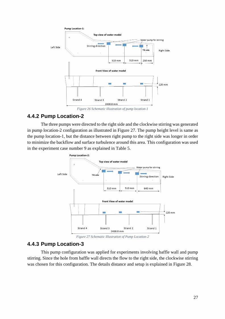
4.4.2 Pump Location-2
The three pumps were directed to the right side and the clockwise stirring was generated
in pump location-2 configuration as illustrated in Figure 27. The pump height level is same as
the pump location-1, but the distance between right pump to the right side was longer in order
to minimize the backflow and surface turbulence around this area. This configuration was used
in the experiment case number 9 as explained in Table 5.
Figure 27 Schematic Illustration of Pump Location-2
4.4.3 Pump Location-3
This pump configuration was applied for experiments involving baffle wall and pump
stirring. Since the hole from baffle wall directs the flow to the right side, the clockwise stirring
was chosen for this configuration. The details distance and setup is explained in Figure 28.

28
Figure 28 Schematic Illustration of Pump Location-3.
4.5 Experimental Method and Setup
Four types of experiments were conducted in this work. Firstly, a velocity mapping was
investigated in order to know the extent of stirring force by water pumps in 30 different
locations within the tundish model. By conducting this measurement, the degree of similarity
between the water pump and EMS can be imagined. Even though it is clear that the pump
stirring is not similar to EMS, at least this measurement can be a foundation to understand the
extent of stirring force that applied in different pump capacity. In addition, it can be a reference
to setup the EMS force in the reality. The second experiment is a flow behavior observation.
The objective is to understand the tendency of flow movement within the tundish. The third
experiment is a salt injection experiment aiming to obtain an RTD Curve for different tundish
configurations. Due to this goal, the RTD experiment term was used to mention this kind of
experiment. The last experiment type is dye color injection, where the flow behavior as well as
the changing of concentration distribution can be observed. In addition, a comparison of mixing
time of each case can also be investigated qualitatively.
4.5.1 Velocity Mapping
The velocity measurement was carried out by a low-velocity meter Nixon flowmeter
430. The measurement tools are displayed in Figure 29. It comprises of a sensing probe of five-
bladed PVC rotor connected to the meter. At the center of the rotor, an insulated gold wire is
installed within a slim tube. The principle of the measurement is when the rotor is moved by a
conductive liquid, the flow passes the gold wire and changes the impedances. This detection is
converted into velocity measurement. The velocity mapping was conducted by measuring 30
different locations. The illustration of measurement points is presented in Figure 30. In this
work, the longitudinal velocity or velocity in x-axes direction was measured for four different
configurations: bare tundish without any stirring and bare tundish with 20%, 30%, and 40% of
water pump capacity.

29
Figure 29 Low velocity meter used in the experiment
Figure 30 Schematic Illustration of measurement point in velocity measurement
4.5.2 Flow Behavior Observation
The flow behavior observation was conducted using a plastic particle which has a
similar density to water. The specific movement in every location was difficult to be observed,
but the general tendency can still be analyzed. The movement of particles at the top surface
from the top view and the right side of tundish model were observed and recorded. This
experiment was conducted for five different configurations, as summarized in Table 5.
4.5.3 RTD Experiment
The RTD experiment procedures are simplified in Figure 31. It was begun by filling the
tundish model and all water tanks with the water from a water tap using pipe P-11, P-12 and
P-13. Then all valves were adjusted to reach the desired volumetric flow rate except V-9 and
V-10 which is kept closed to prevent the water flow to the sink. The circulation of water was
maintained until the desired bath level in the tundish model was reached. Furthermore, the V-
11, V-12 and V-13 were turned off that the water circulation only relies on the water from the
tank. The water flow route is from V-1 to the tundish model, four outlets and then it is circulated
back to the tundish model. This continuous circulation was maintained for 20 minutes to make

30
sure the steady condition and flow pattern is fully generated. Furthermore, a 30 mL of 20%
NaCl as a tracer solution was injected through a syringe connected to the pipe P-2 and valve
V-2. At this time the conductivity meter was turned to record the conductivity data at each
outlet up to 4000 s which is similar around four times of theoretical residence times. Then the
data was transmitted to the computer and the RTD curve was plotted. In total, 13 different
configurations of experiments were conducted by this kind of experiment as summarized in
Table 5.
Figure 31 RTD Experiment Steps
4.5.4 Dye-Color Injection
In this experiment, a 30mL of Dr.Oetker liquid food color was injected at the same location
as salt injection point through a syringe. At the same time, a video was recorded to observe the
changing of concentration gradient inside tundish model. The video was documented until an
approximately homogeneous concentration for the whole tundish achieved. The mixing time
as well as the flow behavior then can be compared qualitatively between different
configurations of the tundish.
4.6 Data Processing Steps of RTD Experiment
In order to analyze the flow behavior at different strands, several flow characteristics such
as: 𝜃𝑚𝑖𝑛, 𝜃𝑝𝑒𝑎𝑘 , 𝐶𝑚𝑎𝑥 , 𝜃𝑚𝑒𝑎𝑛,, fraction of plug flow(𝑽𝒑
𝑽), fraction of dead volume(
𝑽𝒅
𝑽), fraction
of well-mixed volume (𝑽𝒎
𝑽) were calculated from RTD curve. Those flow characteristics can
be obtained using following steps:
1. Run the RTD Experiment up to four times of theoretical residence time and record the
conductivity at each strand.
2. Convert the conductivity value into the concentration (c) based on the relationship as
shown in Figure 32.
3. Determine 𝜃 using Equation 2 and Equation 3.
4. Plot the curve of concentration (c) vs 𝜃 and then determine the area under the curve.
5. Change the concentration (c) into a dimensionless concentration (C) using Equation 4.
6. Plot the C-curve (C vs 𝜃) for each strand and compare each flow characteristics of each
individual strands that have been calculated.
7. 𝜃𝑚𝑖𝑛 and 𝜃𝑝𝑒𝑎𝑘 can be determined from the data of dimensionless time where the tracer
appears for the first time and at the highest concentration value respectively. Meanwhile,
𝜃𝑚𝑒𝑎𝑛 can be calculated based on Equation 5.
8. Determine the plug flow fraction based on Equation 11 using the value obtained from step
(5).
9. In order to obtain the dead volume fraction (𝑉d
𝑉), calculate the cut-off time (𝜃𝑐𝑢𝑡−𝑜𝑓𝑓) then
flow rate through active region (𝑄𝑎
𝑄) using Equation 13 and 16 respectively.

31
10. Using the value obtained from steps (8), the fraction of dead volume can be determined
from Equation 14. The well-mixed volume is then calculated using Equation 18.
11. Calculate and compare the overall tundish performance as well as strand similarity of each
experiment configurations by Equation 19, Equation 20, Equation 21 and Equation 22.
Figure 32 Conductivity vs concentration relationship for a solution of NaCl and water tap at 25℃
4.7 Experiment variables
Four variables were investigated aiming to know the effect of its presence on the tundish
performance. The experiment variables are the existence of flow control devices, namely baffle
wall and turbo-stopper, the three different magnitudes of stirring force by water pump (20%,
30% and 40% of pump capacity) and the stirring direction (clockwise and counterclockwise).
In total, there are13 experiment case number with different configurations and the detail is
explained in Table 5.
y = -3828.7x2 + 1874.1x + 0.2703
0
50
100
150
200
250
0% 3% 5% 8% 10% 13% 15% 18% 20% 23%
Co
nd
uct
ivit
y (m
S/cm
)
NaCl Concentration (wt%)

32
Table 5Experiment Configuration List
Remark:
NS : No Stirring
CC : Counter Clockwise
CW : Clockwise
Case
No
Configuration Experiment Type/ Simulation
Tundish Model Construction Stirring
direction
Pump
Location CFD
Velocity
Mapping
RTD
Experiment
Particle
Movement
Dye
Injection
1 Bare Tundish NS -
2 Bare Tundish + 20% pump capacity CC 1 -
3 Bare Tundish + 30% pump capacity CC 1 - - -
4 Bare Tundish + 40% pump capacity CC 1 - -
5 Tundish + Turbo-stopper NS - - - -
6 Tundish + Turbo-stopper + 20%
pump capacity CC 1 - - - -
7 Tundish + Turbo-stopper + 30%
pump capacity CC 1 - - - -
8 Tundish + Turbo-stopper + 40%
pump capacity CC 1 - - - -
9 Bare Tundish + 20% pump capacity CW 2 - -
10 Tundish + Baffle wall NS 3 -
11 Tundish + Baffle wall + 20% pump
capacity CW 3 - -
12 Tundish + Baffle wall + Turbulence
pad CW - - -
13 Tundish + Baffle wall + Turbulence
pad + 20% pump capacity CW 3 - - - -
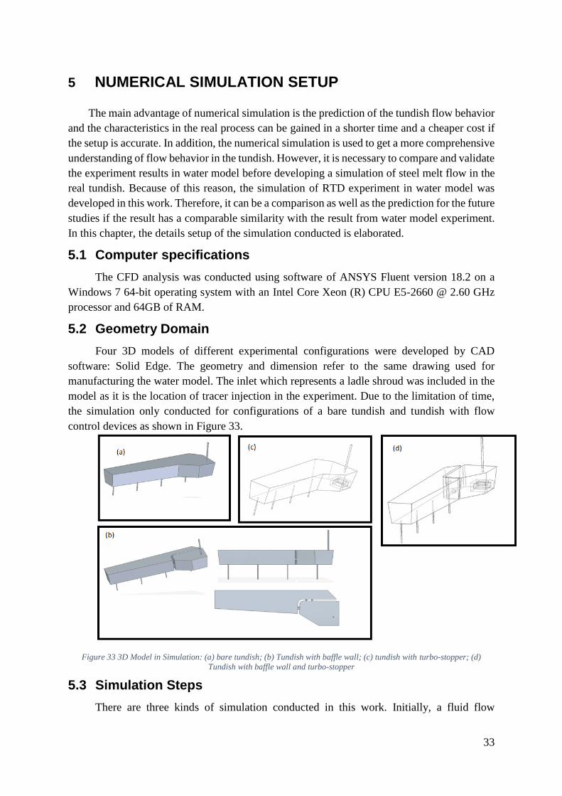
33
5 NUMERICAL SIMULATION SETUP
The main advantage of numerical simulation is the prediction of the tundish flow behavior
and the characteristics in the real process can be gained in a shorter time and a cheaper cost if
the setup is accurate. In addition, the numerical simulation is used to get a more comprehensive
understanding of flow behavior in the tundish. However, it is necessary to compare and validate
the experiment results in water model before developing a simulation of steel melt flow in the
real tundish. Because of this reason, the simulation of RTD experiment in water model was
developed in this work. Therefore, it can be a comparison as well as the prediction for the future
studies if the result has a comparable similarity with the result from water model experiment.
In this chapter, the details setup of the simulation conducted is elaborated.
5.1 Computer specifications
The CFD analysis was conducted using software of ANSYS Fluent version 18.2 on a
Windows 7 64-bit operating system with an Intel Core Xeon (R) CPU E5-2660 @ 2.60 GHz
processor and 64GB of RAM.
5.2 Geometry Domain
Four 3D models of different experimental configurations were developed by CAD
software: Solid Edge. The geometry and dimension refer to the same drawing used for
manufacturing the water model. The inlet which represents a ladle shroud was included in the
model as it is the location of tracer injection in the experiment. Due to the limitation of time,
the simulation only conducted for configurations of a bare tundish and tundish with flow
control devices as shown in Figure 33.
Figure 33 3D Model in Simulation: (a) bare tundish; (b) Tundish with baffle wall; (c) tundish with turbo-stopper; (d)
Tundish with baffle wall and turbo-stopper
5.3 Simulation Steps
There are three kinds of simulation conducted in this work. Initially, a fluid flow

34
simulation was run in order to simulate the fluid flow until reach the steady condition. Then,
the simulation was continued in the transient mode for simulating salt injection experiment.
The last is a simulation of floatation of inclusion by observing particle trajectory from an
injection of inclusion particle. This simulation was also conducted in the transient mode using
the convergence result of fluid flow simulation as the initial condition. The flow work, as well
as the boundary condition of tracer and inclusion injection simulation was elaborated in the
next section.
5.3.1 Tracer Injection Simulation
The summary of tracer injection simulation and its boundary condition was presented in
Figure 34 and Figure 35. The simulation was begun with a fluid flow simulation until reaching
a steady state. Then, the flow and turbulence equation was turned off while the species equation
was activated. Furthermore, the simulation was changed into the transient mode and the tracer
which is a mixture of water and NaCl was injected for a short period of 5s. The simulation
then was run until four times of theoretical residence time. During this period, the concentration
of tracer at each outlet was monitored and extracted in order to obtain an RTD curve.
Figure 34 Steps of salt injection experiment
Figure 35 Boundary condition in tracer injection simulation
5.3.2 Inclusion Injection Simulation
In this simulation, inclusion particles are injected from the inlet and then the amount of
inclusion that trapped on the surface is calculated. As described in Figure 36, the simulation
was started with a simulation of fluid flow until reaching a convergence condition before the
transient mode was activated. The inclusion particles are injected during 2s and the transient
simulation was run until 200s.
Simulation of fluid flow until steady state
Injection of tracer (5s)Transient Simulation up to 4 times of theretical
residence timePlot the results

35
Figure 36 Steps of inclusion injection simulation
Since the water was used as the fluid phase in the simulation instead of hot steel melt
as in the real process, an adjustment of inclusion particle density is necessary to maintain the
similar buoyancy force of inclusion. As a simple approach, the density of inclusion particle
was decided as 560 kg/m3 so that the ratio of inclusion to water density is similar as alumina
inclusion and steel melt in the real process as shown in Table 6.
For boundary condition, a specific interaction between particle and wall was defined.
The surface of the domain was defined as ‘trapped’ while outlets and wall were defined as
‘escaped’ and ‘reflect’ respectively. Thus, a ‘trapped’ surface represent a slag which can react
with inclusion as it is reached the surface. For a details analysis, the surface identity was divided
into two different regions of the surface inside baffle wall (surface 1) and surface outside the
wall (surface 2) for configuration involving baffle wall, as shown in Figure 37.
Table 6 Comparison of fluid-inclusion density in simulation and real industrial tundish
Figure 37 Surface defined as trapped in the configuration: (a) without a baffle wall; (b) and (c) with a baffle wall.
5.4 Simulation List
In this work, a total of eight simulations were run for different objectives as summarized
in Table 7. There are five simulations of bare tundish configurations with different mesh setup
in order to investigate the mesh independence. The rest of simulations were conducted using a
final mesh for simulating the fluid flow, RTD experiment and floatation of inclusion in the
tundish configuration involving flow control devices. As already mentioned previously, the
simulation of pump stirring has not been conducted due to the limitation of time in this work.
Therefore, the analysis from simulation result focuses on the effect of flow control devices.
Simulation of fluid flow until steady state
Injection of inclusion particles (2s)
Transient Simulation for 200s
Observe the results
Material Density (kg/m3) Representation
Steel Melt 7020 Real Industrial Process
Alumina Inclusion 3950
Water 998 CFD Simulation
Inclusion Particle 560
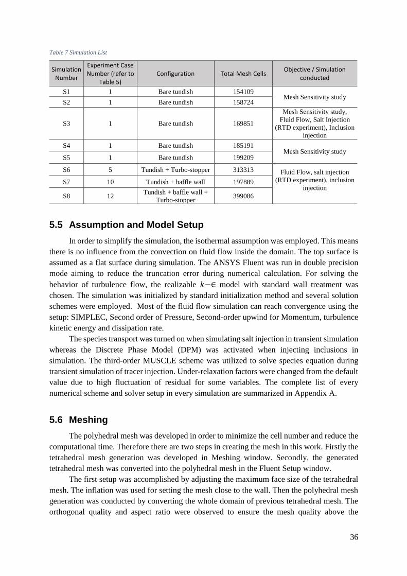
36
Table 7 Simulation List
5.5 Assumption and Model Setup
In order to simplify the simulation, the isothermal assumption was employed. This means
there is no influence from the convection on fluid flow inside the domain. The top surface is
assumed as a flat surface during simulation. The ANSYS Fluent was run in double precision
mode aiming to reduce the truncation error during numerical calculation. For solving the
behavior of turbulence flow, the realizable 𝑘−∈ model with standard wall treatment was
chosen. The simulation was initialized by standard initialization method and several solution
schemes were employed. Most of the fluid flow simulation can reach convergence using the
setup: SIMPLEC, Second order of Pressure, Second-order upwind for Momentum, turbulence
kinetic energy and dissipation rate.
The species transport was turned on when simulating salt injection in transient simulation
whereas the Discrete Phase Model (DPM) was activated when injecting inclusions in
simulation. The third-order MUSCLE scheme was utilized to solve species equation during
transient simulation of tracer injection. Under-relaxation factors were changed from the default
value due to high fluctuation of residual for some variables. The complete list of every
numerical scheme and solver setup in every simulation are summarized in Appendix A.
5.6 Meshing
The polyhedral mesh was developed in order to minimize the cell number and reduce the
computational time. Therefore there are two steps in creating the mesh in this work. Firstly the
tetrahedral mesh generation was developed in Meshing window. Secondly, the generated
tetrahedral mesh was converted into the polyhedral mesh in the Fluent Setup window.
The first setup was accomplished by adjusting the maximum face size of the tetrahedral
mesh. The inflation was used for setting the mesh close to the wall. Then the polyhedral mesh
generation was conducted by converting the whole domain of previous tetrahedral mesh. The
orthogonal quality and aspect ratio were observed to ensure the mesh quality above the
Simulation Number
Experiment Case Number (refer to
Table 5) Configuration Total Mesh Cells
Objective / Simulation conducted
S1 1 Bare tundish 154109 Mesh Sensitivity study
S2 1 Bare tundish 158724
S3 1 Bare tundish 169851
Mesh Sensitivity study,
Fluid Flow, Salt Injection
(RTD experiment), Inclusion
injection
S4 1 Bare tundish 185191 Mesh Sensitivity study
S5 1 Bare tundish 199209
S6 5 Tundish + Turbo-stopper 313313 Fluid Flow, salt injection
(RTD experiment), inclusion
injection
S7 10 Tundish + baffle wall 197889
S8 12 Tundish + baffle wall +
Turbo-stopper 399086

37
minimum requirement of a good mesh. However, for some simulations, several meshes have
orthogonal quality less than 0.1 when generating the tetrahedral mesh. However, those bad
meshess were neglected as the amount is small and the location exist at the unimportant area,
i.e., around the sharp corner of tundish model. The amount, complete setting and mesh quality
used in this work after were summarized in Appendix B.
5.7 Convergence Criteria
The standard criteria for convergence condition of residual for all variables related to
the flow and turbulence equation are less than 10-3 [35]. In this project, convergence criteria of
10-6 were employed to get more accurate steady state results. Meanwhile, the convergence level
10-5 was used for species equation during transient simulation as suggested in ANSYS Fluent
solver setting [36]. Figure 38 shows the simulation that has reached convergence based on this
residual criteria.
Figure 38 Convergence condition of simulation S3
In addition to this observation, several variables were also monitored to ensure a
convergence status has been reached. The volume-average of velocity magnitude, turbulence
related variables, vertex average of velocity at the end of strand 4 and the mass flow rate were
observed. The example of monitoring results is shown in Figure 39 and Figure 40. Based on
those monitoring, it is clear that the simulations have reached convergence as all monitored
variables already have a constant magnitude. Table 8 also shows that the net mass balance is
less than 1% of the smallest flow rate through the domain which also means a convergence
condition has been reached. All those observations were used for all simulations in this work.
Figure 39 Monitor of the average velocity of simulation S3

38
Figure 40 Monitor of velocity at outlet strand 4 of simulations S3
Table 8 Summary of Mass Flow Rate Observation of simulation S1 to S5
Simulation
Number
Mass Flow rate (kg/s)
Inlet Strand 4 Strand 3 Strand 2 Strand 1 Balance
S1 0.3641 -0.09045 -0.09094 -0.09129 -0.09142 -3.51E-08
S2 0.3641 -0.09039 -0.09088 -0.09148 -0.09135 -7.76E-08
S3 0.3641 -0.09009 -0.09094 -0.09155 -0.09152 -8.43E-08
S4 0.3641 -0.09033 -0.09089 -0.09152 -0.09135 -1.17E-07
S5 0.3641 -0.09031 -0.09083 -0.09155 -0.09141 4.94E-09
5.8 Mesh Sensitivity Study
Before analyzing the result of CFD simulation, the mesh sensitivity study was carried
out in order to ensure the grid size independence. This investigation was carried in bare tundish
model. Five different mesh setups were used to compare the volume-average of velocity in
steady state condition. The summary of mesh sensitivity study results was shown in Table 9
and Figure 41. The significant difference between the volume-average of velocity was clearly
observed in simulation number 1, 2 and 3 and the difference decreases gradually from
simulation 3 to simulation 5. Since the relative difference between simulations 3 to 4 is less
than 5%, the grid independence can be concluded has been achieved in simulation 3. Therefore,
the meshing setup of simulation 3 was decided to be used for all simulations in this work. The
final mesh of this setup is displayed in Figure 42.
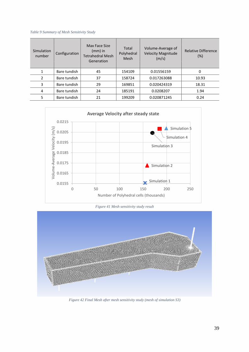
39
Table 9 Summary of Mesh Sensitivity Study
Simulation number
Configuration
Max Face Size (mm) in
Tetrahedral Mesh Generation
Total Polyhedral
Mesh
Volume-Average of Velocity Magnitude
(m/s)
Relative Difference (%)
1 Bare tundish 45 154109 0.01556159 0
2 Bare tundish 37 158724 0.017263088 10.93
3 Bare tundish 29 169851 0.020424319 18.31
4 Bare tundish 24 185191 0.0208207 1.94
5 Bare tundish 21 199209 0.020871245 0.24
Figure 41 Mesh sensitivity study result
Figure 42 Final Mesh after mesh sensitivity study (mesh of simulation S3)
Simulation 1
Simulation 2
Simulation 3
Simulation 4
Simulation 5
0.0155
0.0165
0.0175
0.0185
0.0195
0.0205
0.0215
0 50 100 150 200 250
Vo
lum
e-A
vera
ge V
elo
city
(m
/s)
Number of Polyhedral cells (thousands)
Average Velocity after steady state

40
6 EXPERIMENT RESULTS
6.1 Velocity Mapping
The velocity cannot be detected in all measurement points in a bare tundish
configuration (case 1) due to the very low velocity. Therefore it can be concluded that in
bare tundish configuration without stirring, the fluid is moving very slowly. When the
stirring of 20% pump capacity with counterclockwise direction was introduced (case 2), a
velocity distribution along measurement points appears as shown in Figure 43. The similar
curve of 30% and 40% pump capacity (case 3 and case 4) are provided in Appendix C.
Generally, the area in the center of tundish model specifically at point D to G is the most
affected area since this is the location where pumps installed. The velocity from point A to
J varies from 0.08 to 17.96 cm/s, 0.42 to 20 cm/s and 3.24 to 25.6 cm/s for case 2, 3, and 4
respectively. The average of velocity from the whole measurement points is 7.04, 9.07 and
13.3 cm/s for those case numbers.
Figure 43 Velocity mapping in case 2: bare tundish with stirring (20% capacity and CW direction)
6.2 Flow Behavior Observation
The examples of results from this experiment are presented in Figure 44 to Figure 47.
The plastic particle movement which represents the flow movement is illustrated by the
arrow. Nevertheless, the thickness and length of the arrow do not represent the velocity
magnitude. The top view illustration describes the fluid movement at the top surface while
the Section A-A demonstrates the fluid movement from the right side view of the tundish
model. In Figure 44 a strong inlet jet generates a counterclockwise movement. However,
the fluid moves very slowly from strand 4 to strand 1 so that the stagnant particles were
observed on the right side of tundish model. Meanwhile, examples of the fluid movement
in tundish configuration involving stirring are shown in Figure 45 to Figure 47. In those
cases, there is a strong movement of fluid in the whole tundish even as it creates a strong
backflow on the right side of the tundish. The results of flow behavior are discussed more
comprehensively in section 8 and section 9. Meanwhile, another result of flow illustration

41
in configuration of tundish with baffle wall is provided in Appendix D.
Figure 44 Flow illustration of case no.1: bare tundish
Figure 45 Flow illustration of case no.2: bare tundish + stirring (20% pump capacity, CC direction)
Figure 46 Flow illustration of case no.9: bare tundish + stirring (20% pump capacity and CW direction)
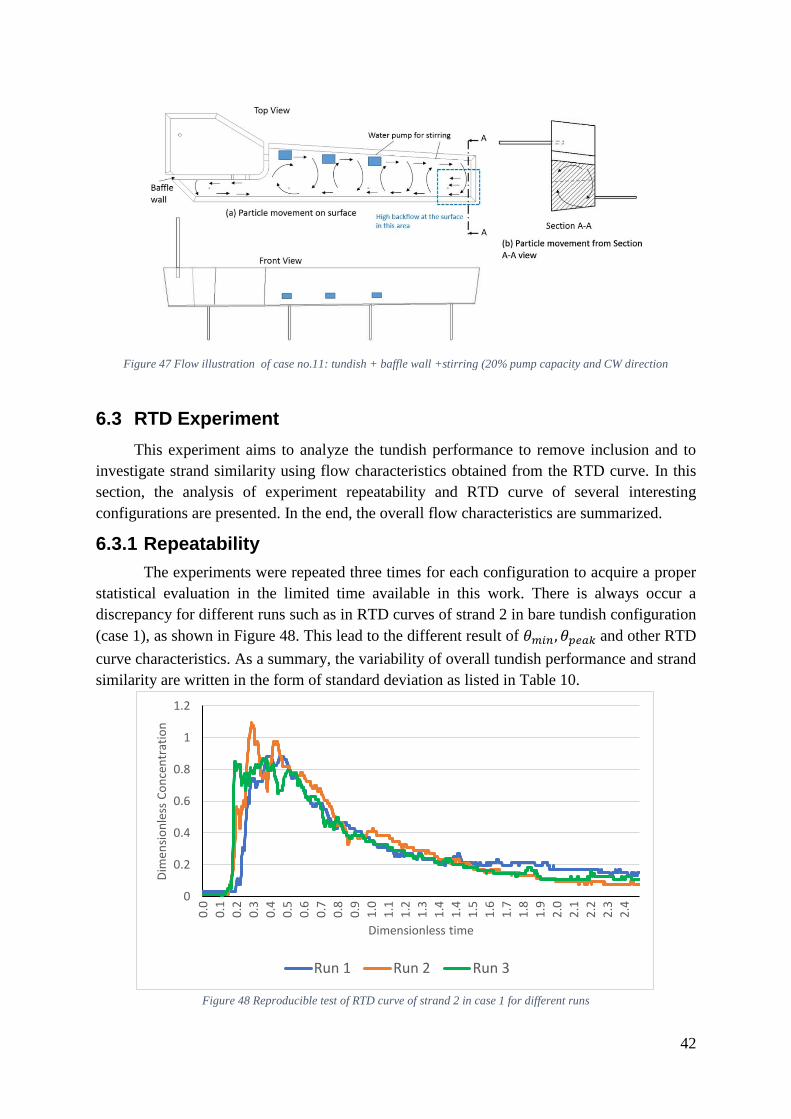
42
Figure 47 Flow illustration of case no.11: tundish + baffle wall +stirring (20% pump capacity and CW direction
6.3 RTD Experiment
This experiment aims to analyze the tundish performance to remove inclusion and to
investigate strand similarity using flow characteristics obtained from the RTD curve. In this
section, the analysis of experiment repeatability and RTD curve of several interesting
configurations are presented. In the end, the overall flow characteristics are summarized.
6.3.1 Repeatability
The experiments were repeated three times for each configuration to acquire a proper
statistical evaluation in the limited time available in this work. There is always occur a
discrepancy for different runs such as in RTD curves of strand 2 in bare tundish configuration
(case 1), as shown in Figure 48. This lead to the different result of 𝜃𝑚𝑖𝑛, 𝜃𝑝𝑒𝑎𝑘 and other RTD
curve characteristics. As a summary, the variability of overall tundish performance and strand
similarity are written in the form of standard deviation as listed in Table 10.
Figure 48 Reproducible test of RTD curve of strand 2 in case 1 for different runs
0
0.2
0.4
0.6
0.8
1
1.2
0.0
0.1
0.2
0.3
0.4
0.5
0.6
0.7
0.8
0.9
1.0
1.1
1.2
1.3
1.4
1.4
1.5
1.6
1.7
1.8
1.9
2.0
2.1
2.2
2.3
2.4
Dim
ensi
on
less
Co
nce
ntr
atio
n
Dimensionless time
Run 1 Run 2 Run 3

43
Table 10 Standard Deviation of Overall Performance of Tundish
Case Number
Standard Deviation
𝑉𝑝
𝑉
𝑉𝑑
𝑉
𝑉𝑚
𝑉 𝑆4
1 10.6% 5.7% 8.9% 18.8%
2 19.0% 10.0% 6.1% 8.2%
3 4.0% 2.4% 1.7% 15.3%
4 14.0% 5.4% 3.3% 0.0%
5 13.8% 6.0% 3.2% 22.8%
6 5.7% 1.7% 1.4% 20.5%
7 9.5% 10.4% 5.6% 24.6%
8 13.6% 2.2% 2.3% 12.4%
9 19.7% 7.7% 7.9% 4.5%
10 3.7% 7.6% 2.9% 3.7%
11 3.0% 2.6% 2.5% 10.4%
12 3.4% 0.4% 1.9% 14.2%
13 4.3% 9.9% 4.9% 15.5%
Most of the important flow characteristics demonstrate a relatively small standard
deviation, namely below 10%. However, there is a high degree of variability for some variables
in certain case number which varies from 10 to 24.6%. This large variation probably occurs
due to many factors such as difference of tracer amount and concentration injected, fluctuation
of the flow rate at inlet and outlets, unstable water tap conductivity, or natural variability of a
transient condition. However, a significant difference of specific variable can still be observed
in two or more cases despite the considerable variability. Therefore a reliable analysis can still
be executed by conducting a proper comparison.
6.3.2 RTD Curve
Several interesting RTD curves of different experiment configuration are presented in this
section. For a configuration without stirring, only a bare tundish configuration (case 1) is
displayed in this section. Figure 49 and Figure 50 displays the RTD curve in case 1 and case
10 while the other configurations involving flow control devices are shown in Appendix E.
Meanwhile Figure 51 to Figure 53 displays the RTD curve in the configuration involving
stirring. Since the RTD curve generated for stirring with different pump capacity have a similar
shape, the only configuration with 20% pump capacity stirring is presented.

44
Figure 49 RTD curve of case 1: bare tundish
Figure 50 RTD curve of case 10: tundish + baffle wall
0.0
0.5
1.0
1.5
2.0
2.5
3.0
3.5
4.0
0.0
0.1
0.3
0.4
0.6
0.7
0.9
1.0
1.1
1.3
1.4
1.6
1.7
1.9
2.0
2.1
2.3
2.4
2.6
2.7
2.9
3.0
3.1
3.3
3.4
3.6
3.7
3.9
4.0
Dim
ensi
on
less
Co
nce
ntr
atio
n
Dimensionless time
Strand 4 Strand 3 Strand 2 Strand 1
0
0.1
0.2
0.3
0.4
0.5
0.6
0.7
0.8
0.9
0.0
0.1
0.3
0.4
0.5
0.7
0.8
1.0
1.1
1.2
1.4
1.5
1.6
1.8
1.9
2.0
2.2
2.3
2.5
2.6
2.7
2.9
3.0
3.1
3.3
3.4
3.6
3.7
3.8
Dim
ensi
on
less
Co
nce
ntr
atio
n
Dimensionless time
Strand 4 Strand 3 Strand 2 Strand 1

45
Figure 51 RTD curve of case 2: bare tundish + stirring (20% pump capacity + CC direction)
Figure 52 RTD Curve of case 9: bare tundish +stirring (20% pump capacity, CW Direction)
0.0
0.5
1.0
1.5
2.0
2.5
3.0
0.0
0.1
0.3
0.4
0.6
0.7
0.8
1.0
1.1
1.2
1.4
1.5
1.7
1.8
1.9
2.1
2.2
2.3
2.5
2.6
2.8
2.9
3.0
3.2
3.3
3.4
3.6
3.7
3.9
4.0
Dim
ensi
on
less
Co
nce
ntr
atio
n
Dimensionless time
Strand 4 Strand 3 Strand 2 Strand 1
0.0
0.5
1.0
1.5
2.0
2.5
3.0
3.5
4.0
4.5
0.0
0.1
0.3
0.4
0.5
0.7
0.8
1.0
1.1
1.2
1.4
1.5
1.6
1.8
1.9
2.0
2.2
2.3
2.5
2.6
2.7
2.9
3.0
3.1
3.3
3.4
3.6
3.7
3.8
4.0
Dim
ensi
on
less
Co
nce
ntr
atio
n
Dimensionless time
Strand 4 Strand 3 Strand 2 Strand 1

46
Figure 53 RTD curve of case 13: tundish + baffle wall + turbo-stopper + stirring (20% pump capacity, CW direction)
6.3.3 Flow Characteristics
Before determining the overall performance of tundish, the flow characteristics of each
strand was calculated and the results are presented in Appendix F. Furthermore, the overall
flow characteristics were calculated using Equation 19, Equation 20 and Equation 21.
Meanwhile, the strand similarity was determined from Equation 22. The summary of overall
tundish performance of all configurations are summarized is in Table 11.
6.4 Dye-Color Injection
The results of color injection experiment for some configurations are presented in Figure
54 to Figure 59. In those figures, the sequence of color concentration changing from the
beginning to the estimated homogeneous concentration reached are displayed. The sequence
displayed in every case is unique depending on the interesting phenomenon observed.
0
0.1
0.2
0.3
0.4
0.5
0.6
0.7
0.8
0.9
0.0
0.1
0.3
0.4
0.6
0.7
0.8
1.0
1.1
1.2
1.4
1.5
1.7
1.8
1.9
2.1
2.2
2.3
2.5
2.6
2.8
2.9
3.0
3.2
3.3
3.4
3.6
3.7
3.9
4.0
Dim
ensi
on
less
Co
nce
ntr
atio
n
Dimensionless time
Strand 4 Strand 3 Strand 2 Strand 1
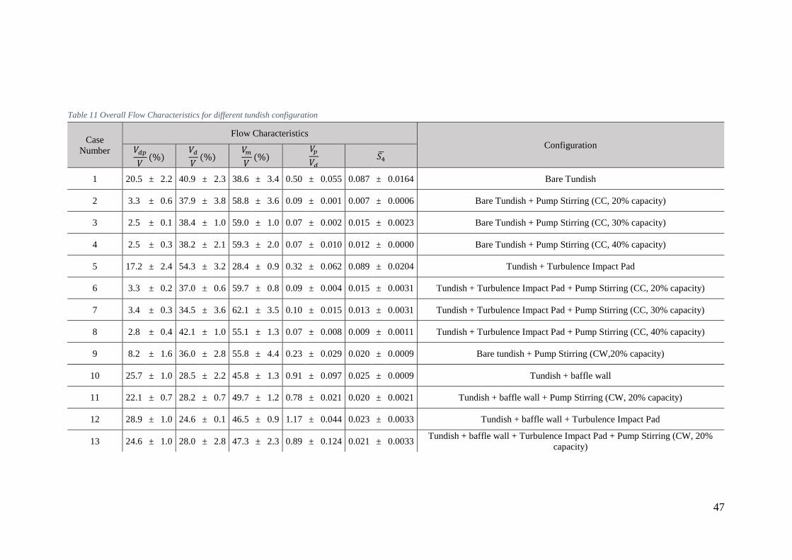
47
Table 11 Overall Flow Characteristics for different tundish configuration
Case
Number
Flow Characteristics
Configuration 𝑉𝑑𝑝
𝑉(%)
𝑉𝑑
𝑉(%)
𝑉𝑚
𝑉(%)
𝑉𝑝
𝑉𝑑
𝑆4
1 20.5 ± 2.2 40.9 ± 2.3 38.6 ± 3.4 0.50 ± 0.055 0.087 ± 0.0164 Bare Tundish
2 3.3 ± 0.6 37.9 ± 3.8 58.8 ± 3.6 0.09 ± 0.001 0.007 ± 0.0006 Bare Tundish + Pump Stirring (CC, 20% capacity)
3 2.5 ± 0.1 38.4 ± 1.0 59.0 ± 1.0 0.07 ± 0.002 0.015 ± 0.0023 Bare Tundish + Pump Stirring (CC, 30% capacity)
4 2.5 ± 0.3 38.2 ± 2.1 59.3 ± 2.0 0.07 ± 0.010 0.012 ± 0.0000 Bare Tundish + Pump Stirring (CC, 40% capacity)
5 17.2 ± 2.4 54.3 ± 3.2 28.4 ± 0.9 0.32 ± 0.062 0.089 ± 0.0204 Tundish + Turbulence Impact Pad
6 3.3 ± 0.2 37.0 ± 0.6 59.7 ± 0.8 0.09 ± 0.004 0.015 ± 0.0031 Tundish + Turbulence Impact Pad + Pump Stirring (CC, 20% capacity)
7 3.4 ± 0.3 34.5 ± 3.6 62.1 ± 3.5 0.10 ± 0.015 0.013 ± 0.0031 Tundish + Turbulence Impact Pad + Pump Stirring (CC, 30% capacity)
8 2.8 ± 0.4 42.1 ± 1.0 55.1 ± 1.3 0.07 ± 0.008 0.009 ± 0.0011 Tundish + Turbulence Impact Pad + Pump Stirring (CC, 40% capacity)
9 8.2 ± 1.6 36.0 ± 2.8 55.8 ± 4.4 0.23 ± 0.029 0.020 ± 0.0009 Bare tundish + Pump Stirring (CW,20% capacity)
10 25.7 ± 1.0 28.5 ± 2.2 45.8 ± 1.3 0.91 ± 0.097 0.025 ± 0.0009 Tundish + baffle wall
11 22.1 ± 0.7 28.2 ± 0.7 49.7 ± 1.2 0.78 ± 0.021 0.020 ± 0.0021 Tundish + baffle wall + Pump Stirring (CW, 20% capacity)
12 28.9 ± 1.0 24.6 ± 0.1 46.5 ± 0.9 1.17 ± 0.044 0.023 ± 0.0033 Tundish + baffle wall + Turbulence Impact Pad
13 24.6 ± 1.0 28.0 ± 2.8 47.3 ± 2.3 0.89 ± 0.124 0.021 ± 0.0033 Tundish + baffle wall + Turbulence Impact Pad + Pump Stirring (CW, 20%
capacity)
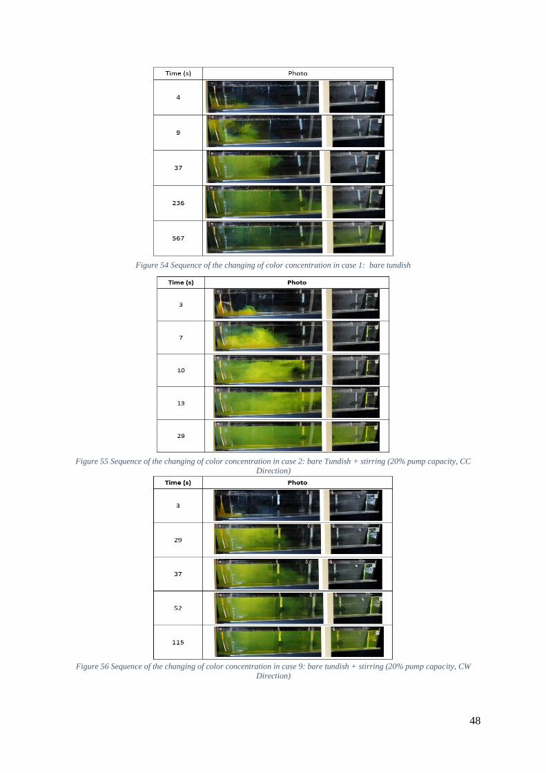
48
Figure 54 Sequence of the changing of color concentration in case 1: bare tundish
Figure 55 Sequence of the changing of color concentration in case 2: bare Tundish + stirring (20% pump capacity, CC
Direction)
Figure 56 Sequence of the changing of color concentration in case 9: bare tundish + stirring (20% pump capacity, CW
Direction)
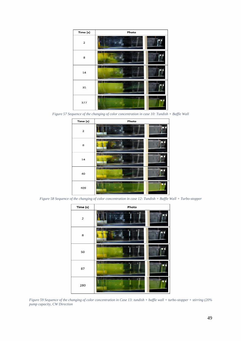
49
Figure 57 Sequence of the changing of color concentration in case 10: Tundish + Baffle Wall
Figure 58 Sequence of the changing of color concentration in case 12: Tundish + Baffle Wall + Turbo-stopper
Figure 59 Sequence of the changing of color concentration in Case 13: tundish + baffle wall + turbo-stopper + stirring (20%
pump capacity, CW Direction
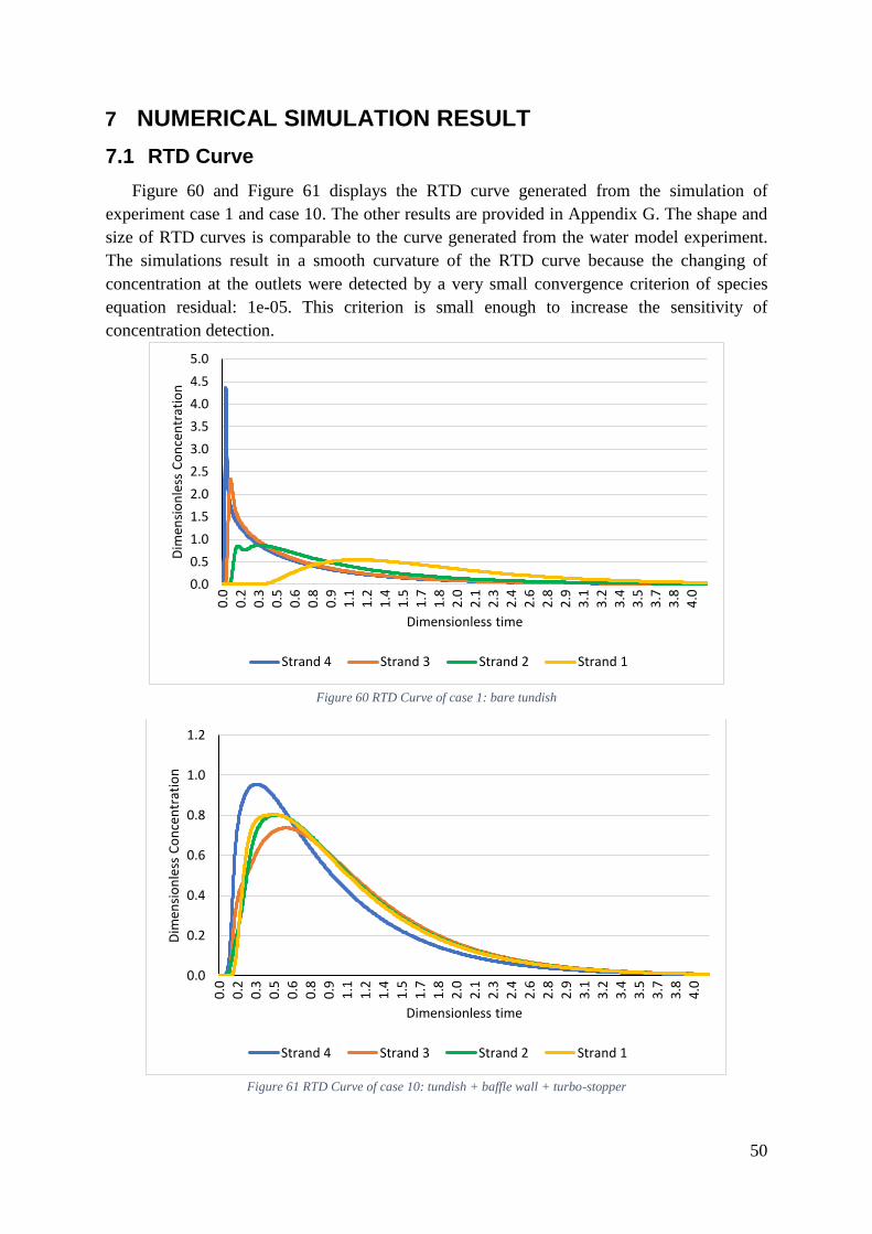
50
7 NUMERICAL SIMULATION RESULT
7.1 RTD Curve
Figure 60 and Figure 61 displays the RTD curve generated from the simulation of
experiment case 1 and case 10. The other results are provided in Appendix G. The shape and
size of RTD curves is comparable to the curve generated from the water model experiment.
The simulations result in a smooth curvature of the RTD curve because the changing of
concentration at the outlets were detected by a very small convergence criterion of species
equation residual: 1e-05. This criterion is small enough to increase the sensitivity of
concentration detection.
Figure 60 RTD Curve of case 1: bare tundish
Figure 61 RTD Curve of case 10: tundish + baffle wall + turbo-stopper
0.0
0.5
1.0
1.5
2.0
2.5
3.0
3.5
4.0
4.5
5.0
0.0
0.2
0.3
0.5
0.6
0.8
0.9
1.1
1.2
1.4
1.5
1.7
1.8
2.0
2.1
2.3
2.4
2.6
2.8
2.9
3.1
3.2
3.4
3.5
3.7
3.8
4.0
Dim
ensi
on
less
Co
nce
ntr
atio
n
Dimensionless time
Strand 4 Strand 3 Strand 2 Strand 1
0.0
0.2
0.4
0.6
0.8
1.0
1.2
0.0
0.2
0.3
0.5
0.6
0.8
0.9
1.1
1.2
1.4
1.5
1.7
1.8
2.0
2.1
2.3
2.4
2.6
2.8
2.9
3.1
3.2
3.4
3.5
3.7
3.8
4.0
Dim
ensi
on
less
Co
nce
ntr
atio
n
Dimensionless time
Strand 4 Strand 3 Strand 2 Strand 1
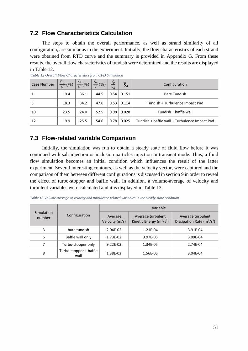
51
7.2 Flow Characteristics Calculation
The steps to obtain the overall performance, as well as strand similarity of all
configuration, are similar as in the experiment. Initially, the flow characteristics of each strand
were obtained from RTD curve and the summary is provided in Appendix G. From these
results, the overall flow characteristics of tundish were determined and the results are displayed
in Table 12. Table 12 Overall Flow Characteristics from CFD Simulation
7.3 Flow-related variable Comparison
Initially, the simulation was run to obtain a steady state of fluid flow before it was
continued with salt injection or inclusion particles injection in transient mode. Thus, a fluid
flow simulation becomes an initial condition which influences the result of the latter
experiment. Several interesting contours, as well as the velocity vector, were captured and the
comparison of them between different configurations is discussed in section 9 in order to reveal
the effect of turbo-stopper and baffle wall. In addition, a volume-average of velocity and
turbulent variables were calculated and it is displayed in Table 13.
Table 13 Volume-average of velocity and turbulence related variables in the steady-state condition
Simulation number
Configuration
Variable
Average Velocity (m/s)
Average turbulent Kinetic Energy (m2/s2)
Average turbulent Dissipation Rate (m2/s3)
3 bare tundish 2.04E-02 1.21E-04 3.91E-04
6 Baffle wall only 1.73E-02 3.97E-05 3.09E-04
7 Turbo-stopper only 9.22E-03 1.34E-05 2.74E-04
8 Turbo-stopper + baffle
wall 1.38E-02 1.56E-05 3.04E-04
Case Number 𝑉𝑑𝑝
𝑉(%)
𝑉𝑑
𝑉(%)
𝑉𝑚
𝑉(%)
𝑉𝑝
𝑉𝑑
Configuration
1 19.4 36.1 44.5 0.54 0.151 Bare Tundish
5 18.3 34.2 47.6 0.53 0.114 Tundish + Turbulence Impact Pad
10 23.5 24.0 52.5 0.98 0.028 Tundish + baffle wall
12 19.9 25.5 54.6 0.78 0.025 Tundish + baffle wall + Turbulence Impact Pad
��𝟒

52
7.4 Results of Inclusion Injection Simulation
In the simulation of inclusion injection, the trajectory of inclusion particles injected was
monitored and the number of particles trapped at the surface was observed. For the simulation
involving baffle wall in the domain, the number of particles trapped is separated for two
different surface definition as already explained in section 5.3.2. In addition, the simulation can
also show the number of inclusion particles escaped to each outlet and the residence time of
each different fate of particles as shown in Table 14.
Table 14 Summary of inclusion injection results
Configuration Fate of Particle
Position No. of
particles Percentage of Particle
Residence time in the tundish
Min Max Average
Bare Tundish
Trapped Surface 1861 84.4% 3.9 198.7 52.8
Escaped Strand 4 126 5.7% 9.1 198.2 75.2
Escaped Strand 3 135 6.1% 4.2 197.4 98.9
Escaped Strand 2 82 3.7% 7.8 196.5 119.3
Escaped Strand 1 0 0.0% 0.0 0.0 0.0
Tundish + Turbo-stopper
Trapped Surface 1876 83.4% 6.1 29.6 29.6
Escaped Strand 4 235 10.4% 47.7 199.1 126.2
Escaped Strand 3 113 5.0% 59.7 192.1 114.3
Escaped Strand 2 25 1.1% 166.5 196.9 184.8
Escaped Strand 1 0 0.0% 0.0 0.0 0.0
Tundish + Baffle Wall
Trapped Surface 1895 90.4% 6.1 198.2 6.3
Escaped Strand 4 56 2.7% 7.1 197.8 138.0
Escaped Strand 3 16 0.8% 110.2 188.7 140.0
Escaped Strand 2 20 1.0% 138.3 198.0 163.5
Escaped Strand 1 110 5.2% 147.6 198.2 172.2
Tundish + Baffle Wall +
Turbo-stopper
Trapped Surface1 68 3.1% 33.9 196.2 99.1
Trapped Surface2 2025 93.3% 6.1 198.6 39.9
Escaped Strand 4 42 1.9% 143.6 196.2 180.0
Escaped Strand 3 5 0.2% 153.8 190.5 175.5
Escaped Strand 2 2 0.1% 131.6 146.0 138.8
Escaped Strand 1 29 1.3% 96.7 198.5 135.1

53
8 EXPERIMENT ANALYSIS
8.1 Velocity Mapping
Figure 62 and Figure 63 displays a combination of several velocity measurement curves at
the different stirring force and different bath level. Two interesting phenomena can be
interpreted from those figures. Firstly, an extremely slow-moving fluid exists in a bare tundish
configuration without any stirring. It is indicated by undetected velocity, or in the other word
the velocity is very close to zero, which reflects a large dead fraction exist in the tundish.
Secondly, the addition of stirring drives the water to move faster. Moreover, a relatively higher
velocity was detected at the area furthest from the inlet. The fluid velocity was also observed
to increase with the increase of pump capacity. Nevertheless, pumps create a local high stirring
force, as shown in Figure 62 by a velocity distribution along the measurement points. The
middle area of the model (between E to G) tend to become the most affected area while the
area near strand 1 (the furthest strand from inlet) becomes the most unaffected area. This means
the velocity at every point is highly dependent on pump location. Therefore, probably the
velocity distribution generated is not precisely similar to EMS. However, the water pump can
still be considered as a good way to model EMS in water model because it generates a similar
macro-stirring as EMS.
The different stirring force was also detected in the vertical direction of the model as
depicted in Figure 63. Velocity detected near the bottom surface (bath level 2) is generally
higher than near the surface (bath level 1) because the pump was located closer to the bottom
than to the surface.
Figure 62 Velocity mapping for different pump stirring force at top side and bath level 2
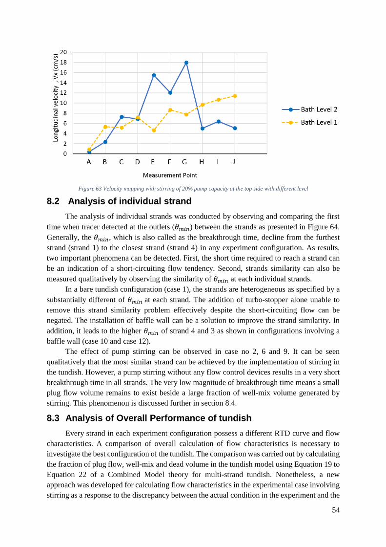
54
Figure 63 Velocity mapping with stirring of 20% pump capacity at the top side with different level
8.2 Analysis of individual strand
The analysis of individual strands was conducted by observing and comparing the first
time when tracer detected at the outlets (𝜃𝑚𝑖𝑛) between the strands as presented in Figure 64.
Generally, the 𝜃𝑚𝑖𝑛, which is also called as the breakthrough time, decline from the furthest
strand (strand 1) to the closest strand (strand 4) in any experiment configuration. As results,
two important phenomena can be detected. First, the short time required to reach a strand can
be an indication of a short-circuiting flow tendency. Second, strands similarity can also be
measured qualitatively by observing the similarity of 𝜃𝑚𝑖𝑛 at each individual strands.
In a bare tundish configuration (case 1), the strands are heterogeneous as specified by a
substantially different of 𝜃𝑚𝑖𝑛 at each strand. The addition of turbo-stopper alone unable to
remove this strand similarity problem effectively despite the short-circuiting flow can be
negated. The installation of baffle wall can be a solution to improve the strand similarity. In
addition, it leads to the higher 𝜃𝑚𝑖𝑛 of strand 4 and 3 as shown in configurations involving a
baffle wall (case 10 and case 12).
The effect of pump stirring can be observed in case no 2, 6 and 9. It can be seen
qualitatively that the most similar strand can be achieved by the implementation of stirring in
the tundish. However, a pump stirring without any flow control devices results in a very short
breakthrough time in all strands. The very low magnitude of breakthrough time means a small
plug flow volume remains to exist beside a large fraction of well-mix volume generated by
stirring. This phenomenon is discussed further in section 8.4.
8.3 Analysis of Overall Performance of tundish
Every strand in each experiment configuration possess a different RTD curve and flow
characteristics. A comparison of overall calculation of flow characteristics is necessary to
investigate the best configuration of the tundish. The comparison was carried out by calculating
the fraction of plug flow, well-mix and dead volume in the tundish model using Equation 19 to
Equation 22 of a Combined Model theory for multi-strand tundish. Nonetheless, a new
approach was developed for calculating flow characteristics in the experimental case involving
stirring as a response to the discrepancy between the actual condition in the experiment and the

55
results from Combined Model theory. In this section, the analysis was conducted using
Combined Model was elaborated while the explanation regarding the new approach of
Combined Model was discussed later in section 8.4.
Figure 64 Effect of experiment configuration on minimum dimensionless time at each strand
8.3.1 Plug Flow
A higher plug flow implies a capability of tundish to give more chances for inclusion
to float towards the surface. As the opposite, a lower plug flow means the flow tends to escape
directly to the outlet without any proper floatation of inclusion. Figure 65 displays the variation
of the fraction of plug flow in different experiment configurations. The highest plug fraction
exhibited by tundish configurations involving baffle wall without any stirring (case 10 and case
12), which means the presence of baffle wall can increase the plug flow fraction significantly.
In the other side, the stirring causes a much smaller plug flow fraction as shown in experiment
case 2-4 and 6-8. The effect of stirring on lowering the plug flow was also observed in the
tundish completed with baffle wall as can be seen in case 9 and 11. This effect occurs due to
the impossibility to gain a tundish with 100% of well-mix volume in stirring cases since the
existence of plug flow cannot be avoided. This phenomenon is discussed deeper in 8.4.
Meanwhile, note case 9 case 2-4 and 6-8 are significantly different, which suggest that the
stirring direction may affect the extent of mixing in the tundish.
0
0.05
0.1
0.15
0.2
0.25
0.3
0.35
0.4
0.45
0 1 2 3 4 5
Min
imu
m D
imen
sio
nle
ss T
ime
Strand
Case 1 (bare tundish)
Case 2 (Bare Tundish + 20% Pump Stirring CC)
Case 5 (Tundish +Turbostopper)
Case 6 (Tundish + Turbostopper + 20%pump stirring CC)
Case 9 (Bare Tundish + 20% Pump Stirring CW)
Case 10 (Tundish + Baffle Wall)
Case 12 (Tundish + Baffle wall + Turbostopper)

56
Figure 65 Fraction of plug flow obtained from Combined Model theory
8.3.2 Dead and Well-Mixed Volume
Figure 66 and Figure 67 present results of the well-mix and the dead volume fraction
determined by Combined Model theory. The well-mix volume increases quite significantly
from the bare tundish configuration (case 1) to the configuration involving baffle wall or
stirring. However, the well-mix and dead volume are unaffected by the addition of turbo-
stopper alone as shown in case 5. On the other hand, the pump stirring, as well as the baffle
wall, reduce the fraction of dead volume.
Unexpectedly, the configuration involving stirring exhibit similar results to configuration
of tundish with baffle wall even though both configurations behave differently during the
experiment. Contrast to baffle wall configuration, the stirring mix the water vigorously and
even create a high fluid circulation. In other words, stirring cases is expected to possess no
slow-moving fluid. Hence, by defining a dead zone in Combined Model as a slowly moving or
stagnant fluid, it can be concluded that Combined Model formula causes an inaccurate flow
fraction in stirring cases. For this argument, the fraction of dead volume in stirring cases
depicted in Figure 67 is still relatively high because the formula considers the fluid flow which
stays over than two times of theoretical residence time as a dead zone. Therefore, a new
approach was developed by the present author to calculate the dead and well-mix volume in
stirring cases. This approach was carried out by modifying the equations in Combined Model
theory and the explanation has been provided in section 8.4.4.
8.3.3 Plug to Dead Zone ratio
One of the purposes of tundish design is to reduce the fraction of dead volume and
increase the fraction of plug flow. A low dead volume is preferred to increase the strand
similarity and avoid the extreme difference of temperature between strands. Meanwhile, a
substantial plug flow indicates a good capability to avoid the short-circuiting flow as well as to
promote a channeling flow for floatation of inclusion. Thus, the plug to dead zone ratio was
used as an indicator for measuring the tundish performance by some researchers [21]. The
results of this ratio for all configurations are presented in Figure 68. The case 10 and case 12
of tundish with the baffle wall seems to be much better than the others. However, the incorrect
0
5
10
15
20
25
30
35
0 1 2 3 4 5 6 7 8 9 10 11 12 13 14
Plu
g FL
ow
Fra
ctio
n (
%)
Case Number
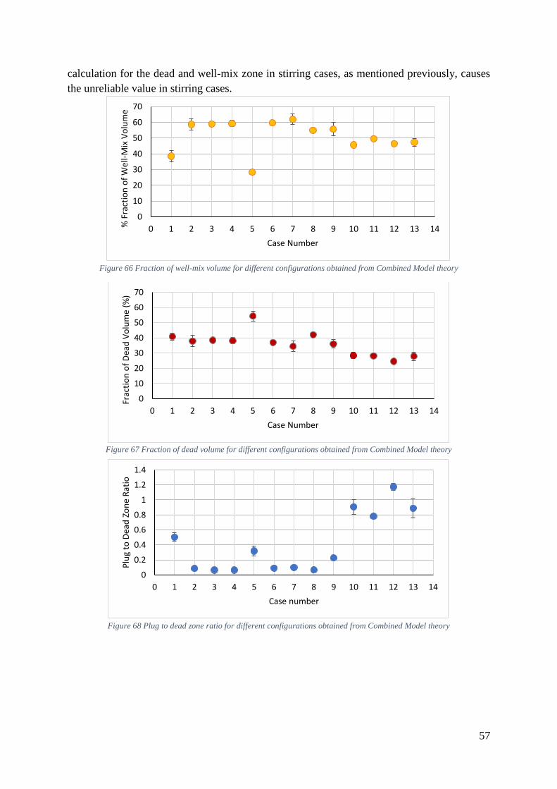
57
calculation for the dead and well-mix zone in stirring cases, as mentioned previously, causes
the unreliable value in stirring cases.
Figure 66 Fraction of well-mix volume for different configurations obtained from Combined Model theory
Figure 67 Fraction of dead volume for different configurations obtained from Combined Model theory
Figure 68 Plug to dead zone ratio for different configurations obtained from Combined Model theory
0
10
20
30
40
50
60
70
0 1 2 3 4 5 6 7 8 9 10 11 12 13 14% F
ract
ion
of
Wel
l-M
ix V
olu
me
Case Number
0
10
20
30
40
50
60
70
0 1 2 3 4 5 6 7 8 9 10 11 12 13 14
Frac
tio
n o
f D
ead
Vo
lum
e (%
)
Case Number
0
0.2
0.4
0.6
0.8
1
1.2
1.4
0 1 2 3 4 5 6 7 8 9 10 11 12 13 14
Plu
g to
Dea
d Z
on
e R
atio
Case number

58
8.4 New Approach of Dead Zone calculation in Stirring Case
As mentioned in the previous chapter, the formula developed by Sahai and Emi of
Combined Model result in the inaccurate fraction of dead and well mix volume for experiment
configuration involving stirring. In this section, the reasons which support that statement are
elaborated and a new approach for calculating the dead and well-mix volume in stirring cases
was proposed.
8.4.1 Reason 1: Fast Moving Fluid
When the stirring applied, the pump generates powerful forces that mix the whole water
in the tundish model. Even high turbulence and backflow observed in some areas in the model.
Thus, it can be concluded that the stirring significantly increases velocity and eliminate the
slow-moving fluid, i.e., dead zone. This conclusion also suggested by the velocity measurement
results which shows a substantial increase in velocity for three different pump capacity as
presented in Figure 55. In addition, the increasing of turbulence also increases the mixing
volume significantly which is undetected by the current formula of Combined Model. Details
explanation regarding the turbulence condition in the model is discussed in section 8.11.
8.4.2 Reason 2: Quick Mixing time
In a color tracer injection experiment, a qualitative comparison of mixing time between
different configurations can be estimated approximately. The mixing time of each
configuration was estimated at the condition where the color tracer has been distributed
homogeneously in the whole tundish as presented in chapter 6.4. On the other hand, the dead
volume existence can also be estimated from the area where the color changed slowly.
Therefore, if the color injected can be mixed very quickly and the homogeneous color
concentration quickly achieved, it can be concluded that there is no dead volume anymore in
the tundish. That is the case that happens in pump stirring configuration as written in Table 15
where the stirring configuration in case 2 only needs 29 s to mix the color homogeneously. It
is much faster compared to the configuration of bare tundish or tundish with a baffle wall which
requires 567 and 377 s respectively to reach a similar condition. The consistent result also
showed in the other cases involving stirring as the faster mixing time than case 1, 10 or 12 can
still be obtained. Based on this observation, it is clear that the velocity of water is much faster
in stirring cases. Therefore, there should be a very high fraction of well-mix volume as the dead
zone does not exist anymore.
Table 15 Summary of estimated mixing time obtained from color injection experiment in different tundish configurations
Case no
Estimated mixing time (s)
Configuration
1 567 Bare tundish
2 29 Tundish with stirring (20% pump capacity, CC direction)
9 115 Tundish with stirring (20% pump capacity, CCW direction)
10 377 Tundish + baffle wall
12 409 Tundish + baffle wall + turbo-stopper
13 280 Tundish + baffle wall + turbo-stopper + stirring (20% pump capacity, CW
direction)

59
8.4.3 Reason 3: Similarity with RTD Curve of Ideal Mix Flow
The argument regarding the influence of pump stirring on the significant increase of
well-mix volume can be understood more clearly from the comparison between two curves of
ideal mix flow and RTD curve involving stirring obtained from the experiment as shown in
Figure 69. In that figure, the ideal mixed flow was determined using equation 9 as explained
in the theory of well-mix flow in chapter 2. Meanwhile, the RTD curve of bare tundish with
20% pump capacity in case 2 was chosen to be compared since the other stirring case also
generates a similar curve.
Unlike the comparison with a bare tundish configuration displayed in Figure 70, it is
apparent that the curvature of ideal mix flow almost fits with the RTD curve from the
experiment involving stirring. It is considered a great similarity which means the pump stirring
results in an almost perfect mixing. However, there is a significant peak observed in the RTD
curve from the experiment which indicates the existence of a very small fraction of plug flow.
Therefore it is impossible to have tundish with 100% of well-mix volume.
Figure 69 Comparison between ideal mix flow and RTD curve from experiment case 2 (type I): tundish + stirring (20%
capacity and CC direction)
It can also be observed that a portion of the fluid which stays more than two times of
theoretical residence times still exist in the ideal mix curve. This dead portion exists not because
of a slow movement, but because there is some portion of the fluid which has a longer traveling
distance covered due to the stirring.
0.0
0.5
1.0
1.5
2.0
2.5
3.0
0.0
0.1
0.3
0.4
0.5
0.7
0.8
0.9
1.1
1.2
1.3
1.5
1.6
1.7
1.9
2.0
2.1
2.3
2.4
2.5
2.7
2.8
2.9
3.1
3.2
3.3
3.5
3.6
3.7
3.9
4.0
Dim
ensi
on
less
Co
nce
ntr
atio
n
Dimensionless timeStrand 4 Strand 3 Strand 2 Strand 1 Ideal Mix Flow

60
Figure 70 Comparison between ideal mix flow and RTD curve from experiment case no.1: bare tundish
8.4.4 Modified Combined Model
Based on the discussion above, the stirring from pumps increase the mixing volume
significantly and annihilate the dead zone. However, the calculation for case no. 2 using
formula developed in Combined Model still results in a contradictive outcome of 58.8% well-
mixed volume and 37.8% dead volume as mentioned in Table 11. Thus, a new approach should
be developed in order to calculate these two flows in all stirring cases more accurately. For this
purpose, a modified combine model was developed and the equations used were shown in
Equation 19, 33 and 34. In this approach, a dead volume is directly determined as 0 because
the slow-moving fluid does not exist anymore. Since the plug flow formula still identical to the
Combined Model theory, then a mixing volume is determined by equation 34. The summary
of the modification in this new approach is illustrated in Figure 71.
𝑉𝑝
𝑉=
1
𝑁(
𝜃1𝑚𝑖𝑛+ 𝜃1𝑝𝑒𝑎𝑘
2) + (
𝜃2𝑚𝑖𝑛+ 𝜃2𝑝𝑒𝑎𝑘
2) + ⋯ . + (
𝜃𝑁𝑚𝑖𝑛+ 𝜃𝑁𝑝𝑒𝑎𝑘
2) Equation 19
𝑉𝑑
𝑉= 0 Equation 34
𝑉𝑚
𝑉= 1 −
𝑉𝑝
𝑉 Equation 35
0.0
0.5
1.0
1.5
2.0
2.5
3.0
3.5
4.0
0.0
0.1
0.3
0.4
0.5
0.7
0.8
0.9
1.1
1.2
1.3
1.5
1.6
1.7
1.9
2.0
2.1
2.3
2.4
2.5
2.7
2.8
2.9
3.1
3.2
3.3
3.5
3.6
3.7
3.9
4.0
Dim
ensi
on
less
Co
nce
ntr
atio
n
Dimensionless time
Strand 4 Strand 3 Strand 2 Strand 1 Ideal Mix Flow

61
Figure 71 A modified combined model used for calculating flow characteristics in stirring cases
8.5 Type of RTD curve in Stirring Case
The new approach of modified Combined Model was employed in all configurations
involving stirring despite there are three different types of RTD curve generated in stirring
cases. Each type indicates a different phenomenon occurred in the experiment. The first type,
or type I, is the RTD curve that demonstrates a very good similarity among the strands and the
curvature almost fits perfectly with the ideal mix curve as already shown in Figure 69. RTD
curve type I occurs in the case number 2, 3, 4, 6, 7 and 8. In this type, the counterclockwise
stirring was successfully distributed the stirring forces homogeneously to all strands as
illustrated in flow behavior in Figure 45.
The second type, which is called type II in this work, is displayed in Figure 72. It is
characterized by one strand, namely the closest strand from the inlet (strand 4), which
experiences a remarkably different behavior compared to the other strands at the beginning of
tracer injection. Even though the difference in strand 4 gradually decreases with the increasing
of time, a slight discrepancy from other strands can still be observed. Figure 72 visualizes the
phenomenon occurred in case 9 where the CW stirring direction is applied on tundish model.
A very tall peak of strand 4 corresponds to the existence of a relatively larger plug flow fraction
compared to the other strands. Meanwhile, a slightly different curvature of strand 4 among the
other strands indicates a different intensity of pump stirring. As depicted in Figure 46, the
stirring forces in the area around strand 4 is a relatively weaker than the other strands because
of the clockwise direction of stirring direct the flow to the right side of tundish model.
Therefore, the velocity of fluid was getting slower when it reaches the area near inlet at the left
side of tundish model.
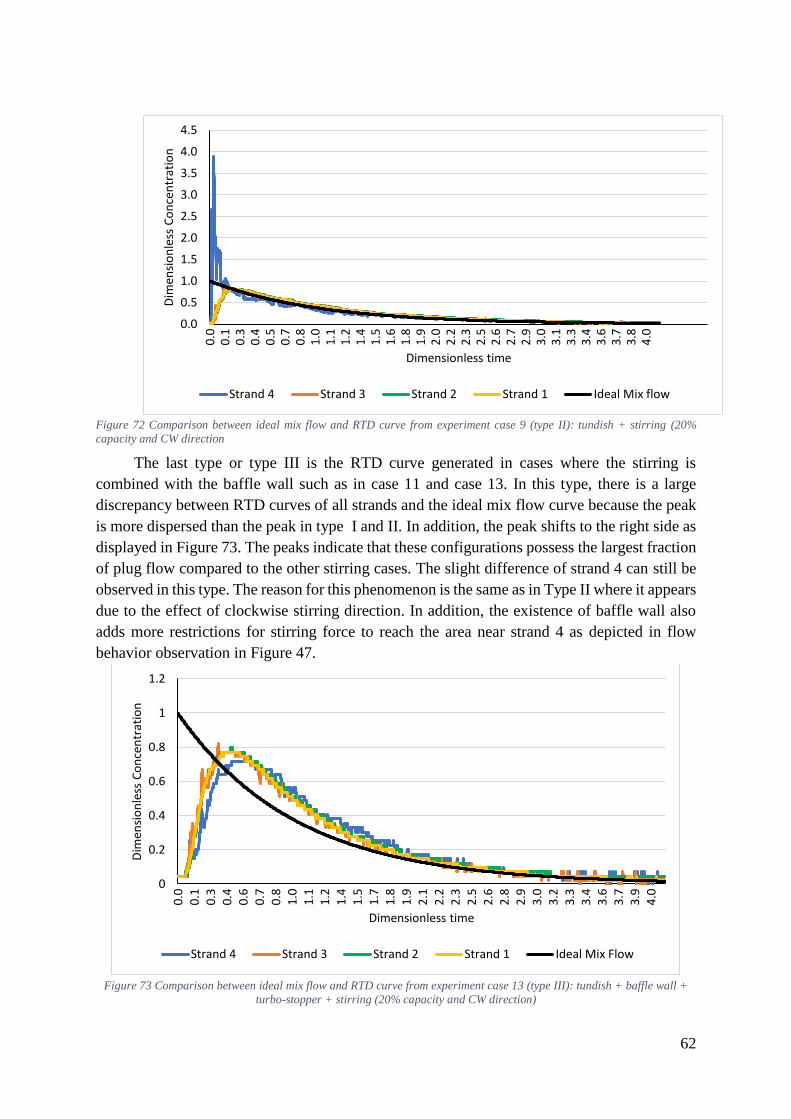
62
Figure 72 Comparison between ideal mix flow and RTD curve from experiment case 9 (type II): tundish + stirring (20%
capacity and CW direction
The last type or type III is the RTD curve generated in cases where the stirring is
combined with the baffle wall such as in case 11 and case 13. In this type, there is a large
discrepancy between RTD curves of all strands and the ideal mix flow curve because the peak
is more dispersed than the peak in type I and II. In addition, the peak shifts to the right side as
displayed in Figure 73. The peaks indicate that these configurations possess the largest fraction
of plug flow compared to the other stirring cases. The slight difference of strand 4 can still be
observed in this type. The reason for this phenomenon is the same as in Type II where it appears
due to the effect of clockwise stirring direction. In addition, the existence of baffle wall also
adds more restrictions for stirring force to reach the area near strand 4 as depicted in flow
behavior observation in Figure 47.
Figure 73 Comparison between ideal mix flow and RTD curve from experiment case 13 (type III): tundish + baffle wall +
turbo-stopper + stirring (20% capacity and CW direction)
0.0
0.5
1.0
1.5
2.0
2.5
3.0
3.5
4.0
4.5
0.0
0.1
0.3
0.4
0.5
0.7
0.8
1.0
1.1
1.2
1.4
1.5
1.6
1.8
1.9
2.0
2.2
2.3
2.5
2.6
2.7
2.9
3.0
3.1
3.3
3.4
3.6
3.7
3.8
4.0
Dim
ensi
on
less
Co
nce
ntr
atio
n
Dimensionless time
Strand 4 Strand 3 Strand 2 Strand 1 Ideal Mix flow
0
0.2
0.4
0.6
0.8
1
1.2
0.0
0.1
0.3
0.4
0.6
0.7
0.8
1.0
1.1
1.2
1.4
1.5
1.7
1.8
1.9
2.1
2.2
2.3
2.5
2.6
2.8
2.9
3.0
3.2
3.3
3.4
3.6
3.7
3.9
4.0
Dim
ensi
on
less
Co
nce
ntr
atio
n
Dimensionless time
Strand 4 Strand 3 Strand 2 Strand 1 Ideal Mix Flow

63
In conclusion, the stirring influences the curvature of RTD curve in all stirring cases so
that it becomes more similar to the ideal mix curve. The only difference in those three types of
RTD Curve types is the amount of plug flow as well as the different stirring intensity at each
strand. Nevertheless, the velocity of the fluid is still considered as fast enough that all strands
contain zero dead zones despite the different of stirring intensity that may happen at a strand.
Therefore, in all stirring cases, the tundish contains a relatively small plug flow and a high
fraction of well-mixed volume as explained in the new approach of Combined Model.
In the other hand, although the strand 4 in Type II and Type III had different mixing
intensity, the formula of well-mix volume in the new approach of Combined Model is assumed
to be valid in both types. It is because in this new approach, the well-mix volume is defined as
a portion of the fluid which has some extent of stirring which means it is independent of the
stirring intensity. As a consequence, the phenomenon of different behavior of strand 4 in type
II and type III cannot be detected by observing the fraction of a well-mix value since it is
possible that a big portion of the well-mixed volume contains some portion of volume with a
weaker stirring intensity. Therefore, a method to detect this ‘non-homogeneous stirring force’
as well as to measure the degree of similarity with ideal mix curve needs to be developed. For
the first mentioned, the strand similarity value (𝑆4) as mentioned in Equation 22 can be used
while for the latter problem, a measure of deviation to the ideal mix curve needs to be
developed. The analysis of these two variables is discussed in section 8.7 and section 8.8
8.6 Analysis of Overall Performance Using the New Approach
Two approaches may be utilized to calculate the overall flow characteristics in the tundish.
The first way is using an old approach or a Combined Model theory where the results are
displayed in Figure 74. In this approach, the Combined Model formula was employed in all
tundish configurations. The second way is the new approach or a modified Combined Model.
This method was developed to improve the accuracy when calculating the fraction of dead and
well-mix volume in configurations involving stirring. As a consequence of this new approach,
a new result of overall flow characteristics in all cases was obtained and it is presented in Figure
75. In this new results, both methods were used: an old approach or a Combined Model was
utilized to calculate the cases without stirring and the modified Combined Model for cases
involving stirring.
Based on the comparison between Figure 69 and Figure 70, it is obvious that there is a big
difference between the dead and well-mix volume fraction in stirring cases. By using the
definition of the dead zone as a slow-moving fluid as proposed by Sahai and Emi [11], it can
be concluded that the results in Figure 69 are inaccurate.
In Figure 75, it is shown that the stirring can exhibit almost 100% of well-mix volume.
However, as mentioned in the previous discussion, the quality of well-mix volume probably
not identical for every strand due to the different extent of stirring intensity reached every
strands. This phenomenon cannot be detected from this result summary, but it is possible to
observe it by analyzing the strand similarity value (𝑆4). Despite good effect to significantly
increase well-mix volume, noticed that the direction of stirring plays a fundamental role in
influencing the results. A change from CC to CW direction in case 9 slightly reduces the well-
mix volume because it affects the amount of plug flow generated inside tundish.
Another interesting fact is it is difficult to create a dominant or full mixing volume since
64
the existence of plug flow cannot be avoided. Therefore it becomes a challenge in stirring cases
to generate fluid flow which allows a bigger fraction of plug flow in order to avoid a short-
circuiting. For this purpose, a new parameter of the plug to well-mix ratio should be calculated
to measure the mixing capability as well as to measure the tendency of short-circuiting flow in
the tundish. This is also useful since the previous parameter used i.e., plug to dead volume ratio
cannot be used anymore due to the zero definition of the dead zone in the new approach for
stirring cases.
8.7 Strand Similarity
Figure 76 presents the similarity among the strands using a strand similarity value (𝑆4)
explained in equation 22. The blue bar represents the value of 𝑆4 in the tundish configuration
with and without flow control devices (baffle wall and turbo-stopper) while the yellow and
brown represent the same parameter in stirring cases but with different stirring direction. A
smaller strand similarity suggests a more homogeneous stirring that the strands quality
becomes more similar to each other.
From the result in Figure 76, it is obvious that the addition of baffle wall increases the
strand similarity significantly as displayed in case 10 and 12. However, an improvement was
presented by the implementation of stirring where the strand similarity is 84% better than in
are tundish configuration (case 1) and 12% better than the configuration involving baffle wall
(case 10 and 12). This result is consistent with the growing of well-mix volume in stirring cases
as presented in Figure 70. Hence, it is proved that a higher mixing is preferred for achieving a
better similarity among strands.
Nevertheless, the stirring direction has a fundamental role which affects the strand
similarity as the 𝑆4 value in CC direction is slightly lower than CW direction. This difference
becomes an indication of the phenomenon happen in RTD curve type II and type II regarding
the strand 4 behavior. Thus, the parameter of 𝑆4 can be used to predict the different intensity
of pump stirring in stirring cases. A lower 𝑆4 value, i.e., 𝑆4 < 0.017, guarantee a better similarity
of strand, and in the other hand, a higher𝑆4, i.e., 𝑆4 >0.017 can be an indication of a different
quality of one or more strands due to different stirring intensity. In addition, this phenomenon
means that careful consideration must be employed to decide the stirring direction as an
appropriate direction can exhibit a very high similarity between strands. The correct stirring
direction depends on the geometry of tundish, steel volume, as well as the EMS location.
8.8 The Similarity with Ideal Mix Curve
The similarity between RTD curves and the ideal mix curve was determined by
calculating the deviation of the area under the RTD curve. In this section, the explanation of
the deviation was presented and the results of all configurations were discussed.

65
Figure 74 Overall flow characteristics using Combined Model theory proposed by Sahai and Emi [19]
20.533.32 2.54 2.49
17.233.35 3.38
2.82 8.23
25.7122.05
28.8824.64
38.62
58.80 59.01 59.28 28.4259.69 62.09
55.08
55.76
45.7849.71
46.52
47.33
40.8537.89 38.45 38.24
54.35
36.96 34.52
42.1036.01
28.50 28.2324.60
28.03
0
20
40
60
80
100
1 2 3 4 5 6 7 8 9 10 11 12 13
Frac
tio
n o
f Fl
ow
Ch
arac
teri
stic
(%
)
Case Number
Plug Volume Well-Mixed Volume Dead Volume

66
Figure 75 Revision of overall flow characteristics after using modified Combined Model in stirring cases
20.533.32
2.54 2.49
17.233.35 3.38 2.82
8.23
25.7122.05
28.8824.64
38.62
96.68 97.46 97.51
28.42
96.65 96.62 97.1891.80
45.78
77.95
46.52
75.36
40.85
54.35
28.5024.60
0
20
40
60
80
100
1 2 3 4 5 6 7 8 9 10 11 12 13
Frac
tio
n o
f Fl
ow
Ch
arac
teri
stic
(%
)
Case Number
Plug Volume Well-Mixed Volume Dead Volume
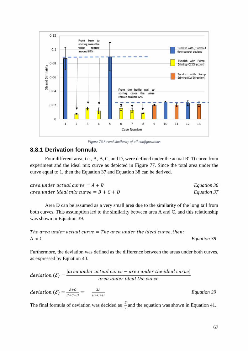
67
Figure 76 Strand similarity of all configurations
8.8.1 Derivation formula
Four different area, i.e., A, B, C, and D, were defined under the actual RTD curve from
experiment and the ideal mix curve as depicted in Figure 77. Since the total area under the
curve equal to 1, then the Equation 37 and Equation 38 can be derived.
𝑎𝑟𝑒𝑎 𝑢𝑛𝑑𝑒𝑟 𝑎𝑐𝑡𝑢𝑎𝑙 𝑐𝑢𝑟𝑣𝑒 = 𝐴 + 𝐵 Equation 36
𝑎𝑟𝑒𝑎 𝑢𝑛𝑑𝑒𝑟 𝑖𝑑𝑒𝑎𝑙 𝑚𝑖𝑥 𝑐𝑢𝑟𝑣𝑒 = 𝐵 + 𝐶 + 𝐷 Equation 37
Area D can be assumed as a very small area due to the similarity of the long tail from
both curves. This assumption led to the similarity between area A and C, and this relationship
was shown in Equation 39.
𝑇ℎ𝑒 𝑎𝑟𝑒𝑎 𝑢𝑛𝑑𝑒𝑟 𝑎𝑐𝑡𝑢𝑎𝑙 𝑐𝑢𝑟𝑣𝑒 = 𝑇ℎ𝑒 𝑎𝑟𝑒𝑎 𝑢𝑛𝑑𝑒𝑟 𝑡ℎ𝑒 𝑖𝑑𝑒𝑎𝑙 𝑐𝑢𝑟𝑣𝑒, 𝑡ℎ𝑒𝑛:
A ≈ C Equation 38
Furthermore, the deviation was defined as the difference between the areas under both curves,
as expressed by Equation 40.
𝑑𝑒𝑣𝑖𝑎𝑡𝑖𝑜𝑛 (𝛿) =|𝑎𝑟𝑒𝑎 𝑢𝑛𝑑𝑒𝑟 𝑎𝑐𝑡𝑢𝑎𝑙 𝑐𝑢𝑟𝑣𝑒 − 𝑎𝑟𝑒𝑎 𝑢𝑛𝑑𝑒𝑟 𝑡ℎ𝑒 𝑖𝑑𝑒𝑎𝑙 𝑐𝑢𝑟𝑣𝑒|
𝑎𝑟𝑒𝑎 𝑢𝑛𝑑𝑒𝑟 𝑖𝑑𝑒𝑎𝑙 𝑡ℎ𝑒 𝑐𝑢𝑟𝑣𝑒
𝑑𝑒𝑣𝑖𝑎𝑡𝑖𝑜𝑛 (𝛿) =𝐴+𝐶
𝐵+𝐶+𝐷=
2𝐴
𝐵+𝐶+𝐷 Equation 39
The final formula of deviation was decided as 𝛿
2 and the equation was shown in Equation 41.

68
𝑑𝑒𝑣𝑖𝑎𝑡𝑖𝑜𝑛 (𝛿
2) =
𝐴
𝐵+𝐶+𝐷=
∑ |𝐶𝑎𝑐𝑡,𝑖−𝐶𝑖𝑑𝑒𝑎𝑙,𝑖|𝑥 𝑑𝜃𝑁𝑖=1
𝐶𝑖𝑑𝑒𝑎𝑙,𝑖 𝑥 𝑑𝜃=
∑ |𝐶𝑎𝑐𝑡,𝑖−𝐶𝑖𝑑𝑒𝑎𝑙,𝑖|𝑁𝑖=1
𝐶𝑖𝑑𝑒𝑎𝑙,𝑖 Equation 40
By this definition, the closer 𝛿
2 value to 0, the more similar the RTD curve to the ideal mix
curve.
Figure 77 Deviation of area under the actual RTD curve and the ideal mix curve
8.8.2 Analysis of deviation from ideal mix
The deviation to the ideal mix ( 𝛿
2 ) of all strands for all configurations is summarized in
Table 16. The stirring not only causes the strands becomes more similar each other, but also it
become more similar to the ideal mix curve as a low 𝛿
2 found in all configurations of bare
tundish with stirring or in combination with a turbo-stopper (case 2-4 and case 6-8). However,
the similar result cannot be achieved by the addition of baffle wall as a higher 𝛿
2 observed in
case 11 and 13. This result is consistent with the RTD curve obtained from the experiment, i.e.,
RTD curve type III. In such RTD curve, the ideal mix curve is clearly not identical to the RTD
curve of all strands because of a relatively high fraction of plug flow results in a broader and
right-shifted peak. Meanwhile, noticed that the 𝛿
2 in stirring cases with a baffle wall (case 11
and case 13) and in baffle wall configuration (case 10 and case 12) are insignificantly different
to the bare tundish (case 1). It is strange considering the RTD in bare tundish should exhibit a
great difference with the ideal mix curve as already shown in Figure 65. Therefore, the 𝛿
2 value
cannot successfully describe the deviation to ideal mix in any configurations without stirring
as this approach cannot detect the difference of curvature in RTD curve.

69
Table 16 Deviation from ideal mix for all configurations
8.9 Plug to Well-Mix Volume ratio
The plug to well-mix ratio, which is also suggested to measure the performance of
tundish by Ahuja and Sahai [21], is a replacement for the similar parameter of the plug to dead
zone ratio. This replacement is necessary since after the revision from Combine Model to the
new approach, the previous ratio becomes invalid due to zero dead zone in all stirring cases. A
careful analysis should be considered when observing this ratio because in one side a higher
plug flow is preferred to promote floatation of inclusion, and in the other side a higher mixing
volume is also worthy for strand similarity.
Figure 78 shows the summary of this variable for all configurations. It can be seen that all
stirring cases in bare tundish with and without a turbo-stopper (case 2-4 and case 6-9) have the
lowest ratio since the tundish consists of very low plug flow and an extremely high well-mix
volume. Interestingly, the insignificant difference was observed between the unstirred
configuration of bare tundish with (case 10 and case 12) and without a baffle wall (case 1 and
case 5). Such insignificant difference happens because both of plug flow and well-mix volume
increases if the baffle wall is installed. Such result exposes a difficulty in determining an ideal
value of this ratio. Therefore, ranges of the optimal plug to the well-mix ratio for ideal tundish
need to be investigated further.
Case
no.
Deviation ( 𝛿
2 )
Configuration Strand
4
Strand
3
Strand
2
Strand
1 Average
1 20.1% 16.8% 16.5% 30.2% 20.9% Bare Tundish
2 6.7% 7.5% 7.6% 7.2% 7.3% Bare Tundish + Stirring (20% pump capacity
and CC direction)
3 5.9% 3.8% 5.2% 4.0% 4.7% Bare Tundish + Stirring (30% pump capacity
and CC direction)
4 8.6% 11.5% 10.2% 10.1% 10.1% Bare Tundish + Stirring (40% pump capacity
and CC direction)
5 24.5% 29.0% 20.4% 24.5% 24.6% Tundish + Turbo-stopper
6 6.1% 9.8% 7.3% 7.4% 7.6% Tundish + Turbo-stopper + Stirring (20%
pump capacity and CC Direction)
7 5.2% 6.6% 5.0% 6.9% 5.9% Tundish + Turbo-stopper + Stirring (30%
pump capacity and CC Direction)
8 9.9% 10.0% 9.0% 10.7% 9.9% Tundish + Turbo-stopper + Stirring (40%
pump capacity and CC Direction)
9 9.1% 9.2% 10.8% 8.9% 9.5% Bare Tundish + Stirring (20% pump capacity
and CW direction)
10 19.1% 21.8% 14.7% 15.6% 17.8% Tundish + Baffle Wall
11 19.0% 15.0% 16.1% 14.9% 16.2% Tundish + Baffle Wall + Stirring (20% pump
capacity and CW Direction)
12 21.4% 23.3% 19.3% 18.7% 20.7% Tundish + Baffle Wall + Turbo-stopper
13 21.0% 16.7% 18.9% 16.7% 18.3%
Tundish + Baffle Wall + Turbo-stopper
Stirring (20% pump capacity and CW
Direction)
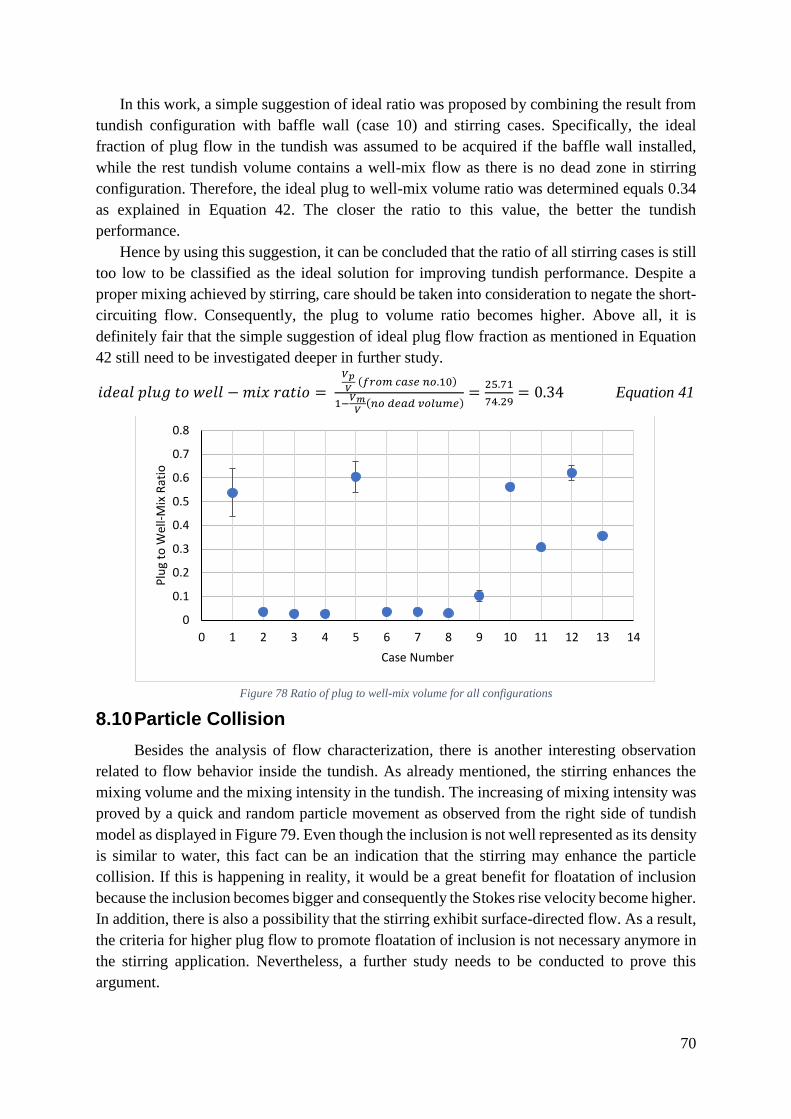
70
In this work, a simple suggestion of ideal ratio was proposed by combining the result from
tundish configuration with baffle wall (case 10) and stirring cases. Specifically, the ideal
fraction of plug flow in the tundish was assumed to be acquired if the baffle wall installed,
while the rest tundish volume contains a well-mix flow as there is no dead zone in stirring
configuration. Therefore, the ideal plug to well-mix volume ratio was determined equals 0.34
as explained in Equation 42. The closer the ratio to this value, the better the tundish
performance.
Hence by using this suggestion, it can be concluded that the ratio of all stirring cases is still
too low to be classified as the ideal solution for improving tundish performance. Despite a
proper mixing achieved by stirring, care should be taken into consideration to negate the short-
circuiting flow. Consequently, the plug to volume ratio becomes higher. Above all, it is
definitely fair that the simple suggestion of ideal plug flow fraction as mentioned in Equation
42 still need to be investigated deeper in further study.
𝑖𝑑𝑒𝑎𝑙 𝑝𝑙𝑢𝑔 𝑡𝑜 𝑤𝑒𝑙𝑙 − 𝑚𝑖𝑥 𝑟𝑎𝑡𝑖𝑜 =
𝑉𝑝
𝑉 (𝑓𝑟𝑜𝑚 𝑐𝑎𝑠𝑒 𝑛𝑜.10)
1−𝑉𝑚
𝑉(𝑛𝑜 𝑑𝑒𝑎𝑑 𝑣𝑜𝑙𝑢𝑚𝑒)
=25.71
74.29= 0.34 Equation 41
Figure 78 Ratio of plug to well-mix volume for all configurations
8.10 Particle Collision
Besides the analysis of flow characterization, there is another interesting observation
related to flow behavior inside the tundish. As already mentioned, the stirring enhances the
mixing volume and the mixing intensity in the tundish. The increasing of mixing intensity was
proved by a quick and random particle movement as observed from the right side of tundish
model as displayed in Figure 79. Even though the inclusion is not well represented as its density
is similar to water, this fact can be an indication that the stirring may enhance the particle
collision. If this is happening in reality, it would be a great benefit for floatation of inclusion
because the inclusion becomes bigger and consequently the Stokes rise velocity become higher.
In addition, there is also a possibility that the stirring exhibit surface-directed flow. As a result,
the criteria for higher plug flow to promote floatation of inclusion is not necessary anymore in
the stirring application. Nevertheless, a further study needs to be conducted to prove this
argument.
0
0.1
0.2
0.3
0.4
0.5
0.6
0.7
0.8
0 1 2 3 4 5 6 7 8 9 10 11 12 13 14
Plu
g to
Wel
l-M
ix R
atio
Case Number

71
Figure 79 Illustration and actual photo of particle collision from the right view of tundish in stirring application
8.11 Surface Condition
Despite the positive effect of pump stirring on increasing mixing volume, attention should
be taken into consideration regarding surface turbulence condition. Relatively low surface
turbulence observed at the surface of tundish with stirring of 20% pump capacity (Figure 80-
a) and stronger surface turbulence was observed when the stirring force changed into 30%
pump capacity (Figure 80-b). Although the pump stirring is not exactly similar to EMS in
reality and the pump position in different bath level highly affects the surface condition, a
careful setup should be measured when implementing stirring in the tundish as a relatively calm
surface is preferred to negate the slag entrainment.
In addition, the consideration of stirring direction selection is also vital because it may
affect the surface condition. Since the tundish shape in this work is asymmetrical, i.e., the
volume in the right side is smaller than in the left side, a high backflow was observed when
implementing a clockwise stirring direction as presented in Figure 80-c and Figure 80-d. Such
unstable surface condition around the corner is vulnerable to the slag entrainment in the real
industrial process.

72
Figure 80 Surface condition observed in stirring configuration: (a) with 20% pump capacity; (b) with 30% pump capacity;
(c) and (d) high backflow in the right side of tundish.
8.12 Ethical and Social Aspect Consideration
Based on the previous discussion it is clear that the stirring has many positive advantages
for increasing tundish performance although attention regarding the surface condition should
be taken into consideration. Concerning to the ethical and social aspect, the work conducted in
this project does not violate any ethical issues as it does not harm any person or any company
which relates to this technology. Even the EMS technology may give benefit to the society
since it helps the steelmaking company to improve their product quality and work efficiency.
This means the EMS technology, which is modelled in this work, is feasible to be implemented
in the real industrial casting process.

73
9 NUMERICAL SIMULATION ANALYSIS
The CFD simulation conducted in this work can be used for predicting the results in the
real industrial tundish if reliable results obtained. Therefore, some comparison between the
experiment and simulation results were presented in this chapter to validate the simulation
results. Furthermore, the effect of baffle wall and turbo-stopper were also investigated by
analyzing some variables that are difficult to be observed in the water model experiment. In
addition, a simulation of inclusion injection was also elaborated to give more comprehensive
analysis regarding the role of those two flow control devices.
9.1 Wall Y+ Problem
Before analyzing the result, the wall Y+ were checked to acquire the idea regarding the
validity of simulation around the wall. Since a Standard Wall Treatment used in the simulation
setup, the valid wall Y+ value should range from 30 to 300. The simulation results show that
there are some invalid wall Y+ as shown in Figure 81. However, since the mixing in the tundish
is the interest phenomena rather than the forces acting around the wall, the effect of invalid
wall Y+ was neglected. In addition, in such a big volume of the multi-strand tundish, the mixing
phenomena is independent of forces around the wall.
Figure 81 Wall Y value of Simulation number 1: Bare Tundish
9.2 Validation of CFD Simulation
Several comparisons between the experiment and simulation result were discussed in this
section as a way to validate the simulation result. The validation was examined in three
different experiment: color injection experiment, particle movement and RTD experiment. The
first two validation give a qualitative comparison while the last validation gives a quantitative
judgement.
9.2.1 Validation of Color Tracer Injection
Figure 82 and Figure 83 show a comparison of the concentration gradient of tracer
during color injection for a different flow time. In bare tundish simulation, the tracer moves
very slowly without any help from external force except inlet jet. Thus the tracer can only reach
the first-two strand after 37s. At this time, the contour of concentration gradient is slightly
different with experiment. Then the tracer travels to the right side of tundish with a higher

74
velocity around the bottom surface as also observed in the experiment.
A more similar comparison was observed in case 10 of tundish with the baffle wall. In
this case, a little amount of color appears from the inclined holes of the baffle wall at 14s before
a much higher concentration flow through these holes as detected at 35s. Both experiment and
simulation show the homogeneous condition is approximately reached at 377s. Based on these
two comparisons, it can be concluded that the simulation was successfully described the
tendency of concentration distribution during color injection the experiment. Therefore, a valid
and reliable result can be obtained.
Figure 82 Comparison between color injection experiment and simulation result in case no.1: bare tundish configuration
Figure 83 Comparison between color injection experiment and simulation result in simulation no.3: Tundish + baffle wall
9.2.2 Validation of Prediction Regarding Dead Zone Location
Even though the fraction of dead volume can be determined by calculating a portion of
fluid stays over than two times of theoretical residence time as explained in Combined Model,
the location is still unknown. The problem to determine the dead zone location can be solved

75
by numerical simulation. As the dead zone is defined as a slow-moving or stagnant fluid [19],
the prediction of dead zone location was determined by showing the area where the slow
velocity fluid exists.
As mentioned in Table 13, the simulation of bare tundish configuration specified that
average of velocity in the whole tundish in steady condition was 0.02 m/s. Hence, in this work,
a very slow-moving fluid is defined as the fluid which has the velocity less than 10% of the
average which displayed as the green area in Figure 84. The results show that most dead zones
exist at the area located around the two-furthest strand, i.e., strand 2 and 1 and it suits the result
from particle movement observation in the water model experiment, where the stagnant particle
exists at the right side of the tundish. Based on this validation, it can be concluded that the
result of velocity contour was also reliable to be analyzed.
Figure 84 Comparison of slow-moving fluid in the particle movement observation (top) and simulation (bottom)
9.2.3 Validation of RTD Curve and Flow Characteristics
The discrepancy between the experiment and simulation result was also observed in RTD
curve, as occurred in a bare tundish configuration shown in Figure 85 and tundish with the
baffle wall shown in Figure 86. In the first case, the clear difference was found at several
variables such as the maximum concentration, area under the curve, and minimum nor peak
dimensionless time (𝜃min and 𝜃𝑝𝑒𝑎𝑘) of each strand. However, a general tendency of RTD
curve between each strand seemed similar, as the closer strand from the inlet always appears
earlier before the further strand. In addition, a short-circuiting flow phenomenon clearly can be
detected in both experiment and simulation.
In the baffle wall configuration, even though there is a slight difference in term of the
sequence of tracer appearance among strands, the curves from experiment and simulation have
a relatively great similarity in total area under the curve, strand similarity as well as maximum

76
peak. In conclusion, some degree of similarity can be found between the RTD curve from
experiment and simulation. However, the discrepancy of the RTD curve generated in
experiment and simulation still leads to the difference of flow characteristics as quantified in
Table 17.
Figure 85 Comparison of RTD curves obtained from experiment and simulation in bare tundish configuration (case 1)
Figure 86 Comparison of RTD curves obtained from experiment and simulation in the tundish with baffle wall (case 10)
0
0.5
1
1.5
2
2.5
3
3.5
4
4.5
5
0.0
0.1
0.1
0.2
0.3
0.3
0.4
0.4
0.5
0.6
0.6
0.7
0.8
0.8
0.9
0.9
1.0
1.1
1.1
1.2
1.3
1.3
1.4
1.4
1.5
1.6
1.6
1.7
1.8
1.8
1.9
1.9
Dim
ensi
on
less
Co
nce
ntr
atio
n
Dimensionless time
Strand 4 (Exp) Strand 3 (Exp) Strand 2 (Exp) Strand 1 (Exp)
ST 4 (Sim) ST 3 (Sim) ST 2 (Sim) ST 1 (Sim)
0
0.2
0.4
0.6
0.8
1
1.2
0.0
0.1
0.1
0.2
0.3
0.3
0.4
0.4
0.5
0.6
0.6
0.7
0.8
0.8
0.9
0.9
1.0
1.1
1.1
1.2
1.3
1.3
1.4
1.4
1.5
1.6
1.6
1.7
1.8
1.8
1.9
1.9
Dim
ensi
on
less
Co
nce
ntr
atio
n
Dimensionless time
Strand 4 (Exp) Strand 3 (Exp) Strand 2 (Exp) Strand 1 (Exp)
ST 4 (Sim) ST 3 (Sim) ST 2 (Sim) ST 1 (Sim)

77
Table 17 the difference of flow characteristics from experiment and simulation
Based on the comparison in Table 17, it was observed that the result of flow
characteristics vary from a relatively small difference of 5.27% to a huge difference of 67.43%.
The difference which is less than 10% are believed as a reliable result while the rest means the
simulation cannot describe the reality in the experiment accurately.
However, despite the large discrepancies observed, the general effect of the addition of
flow control devices addition on certain flow characteristics can still be predicted by
simulation. The examples are the growing of the well-mix volume, the improvement of strand
similarity, and the decreasing of the dead zone which can be observed after the addition of
baffle wall. However, a contradictive result from experiment and simulation was found in the
configuration involving turbo-stopper. The discrepancy between experiment and simulation
may be caused by the simplification of the radius inside the turbo-stopper when developing the
3D model in simulation. The other factor is probably caused by inappropriate turbulence model
and wall Y+ value inside the turbo-stopper because of the strong turbulence and circulation.
9.3 Effect of Baffle wall
One of the main advantages of the baffle wall used in this work is the inclined holes
which direct the flow towards the surface. This effect was clearly shown in Figure 87, where
the tracer only needs 14s to reach the surface. The other benefit is the baffle wall has three
holes which serve to distribute the flow to different strands properly. This outcome was
displayed in Figure 88, where one hole direct the flow towards the strands 2 and 1 on the right
side of the tundish and the other two holes distribute the melt to the two-closer strand from the
inlet. Lastly, the baffle wall plays an important role to avoid the fluid flow directly to the strand
4 without any proper mixing inside the baffle wall as displayed in Figure 89.
Case Number Flow Characteristics Result
%Difference Experiment CFD Simulation
1
Plug flow fraction (%) 20.5 19.4 5.27%
Dead volume fraction (%) 40.9 36.1 11.66%
Well-mix volume fraction (%) 38.6 44.5 -15.13%
Plug to Dead Zone Ratio 0.50 0.53 -7.06%
Strand similarity 0.087 0.150 -73.24%
5
Plug flow fraction (%) 17.2 18.3 -6.01%
Dead volume fraction (%) 54.4 34.2 37.16%
Well-mix volume fraction (%) 28.4 47.6 -67.43%
Plug to Dead Ratio 0.32 0.53 -67.39%
Strand similarity 0.090 0.114 -27.52%
10
Plug flow fraction (%) 25.7 23.5 8.47%
Dead volume fraction (%) 28.5 23.9 15.92%
Well-mix volume fraction (%) 45.8 52.5 -14.67%
Plug to Dead Zone Ratio 0.91 0.98 -8.28%
Strand similarity 0.024 0.028 -14.19%
12
Plug flow fraction (%) 28.9 19.9 30.99%
Dead volume fraction (%) 24.6 25.4 -3.51%
Well-mix volume fraction (%) 46.5 54.6 -17.38%
Plug to Dead Zone Ratio 1.17 0.78 33.34%
Strand similarity 0.022 0.025 -9.77%

78
Figure 87 effect of baffle wall: surface-directed flow
Figure 88 Effect of the baffle holes on the flow distribution among strands
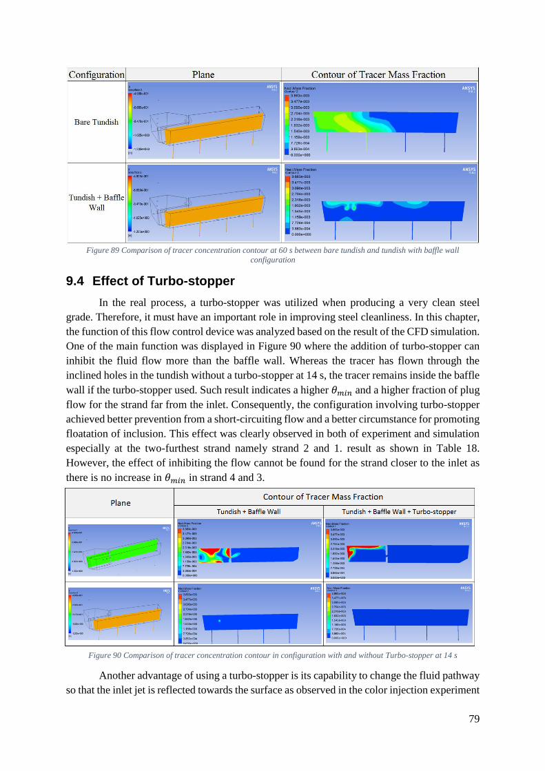
79
Figure 89 Comparison of tracer concentration contour at 60 s between bare tundish and tundish with baffle wall
configuration
9.4 Effect of Turbo-stopper
In the real process, a turbo-stopper was utilized when producing a very clean steel
grade. Therefore, it must have an important role in improving steel cleanliness. In this chapter,
the function of this flow control device was analyzed based on the result of the CFD simulation.
One of the main function was displayed in Figure 90 where the addition of turbo-stopper can
inhibit the fluid flow more than the baffle wall. Whereas the tracer has flown through the
inclined holes in the tundish without a turbo-stopper at 14 s, the tracer remains inside the baffle
wall if the turbo-stopper used. Such result indicates a higher 𝜃𝑚𝑖𝑛 and a higher fraction of plug
flow for the strand far from the inlet. Consequently, the configuration involving turbo-stopper
achieved better prevention from a short-circuiting flow and a better circumstance for promoting
floatation of inclusion. This effect was clearly observed in both of experiment and simulation
especially at the two-furthest strand namely strand 2 and 1. result as shown in Table 18.
However, the effect of inhibiting the flow cannot be found for the strand closer to the inlet as
there is no increase in 𝜃𝑚𝑖𝑛 in strand 4 and 3.
Figure 90 Comparison of tracer concentration contour in configuration with and without Turbo-stopper at 14 s
Another advantage of using a turbo-stopper is its capability to change the fluid pathway
so that the inlet jet is reflected towards the surface as observed in the color injection experiment

80
as well as the concertation contour from simulation in Figure 91. Moreover, a strong circulation
formed inside the turbo-stopper enhances a proper mixing and inclusion collision before the
melt moves through the hole of baffle wall as shown by strong circulation vector below inlet
jet in Figure 92.
Table 18 Comparison of minimum dimensionless time from experiment and simulation between case 10 and case 12
Strands
Minimum Dimensionless time
Tundish + baffle wall (case 10) Tundish + baffle wall + Turbo-stopper (case 12)
Experiment Simulation Experiment Simulation
1 0.0897 0.0185 0.1324 0.0277
2 0.0975 0.0164 0.1287 0.0164
3 0.1047 0.0144 0.1376 0.0133
4 0.0852 0.0123 0.0122 0.0123
Figure 91 Effect of turbo-stopper on creating surface-directed flow
Figure 92 Velocity vector below inlet jet

81
9.5 Dead Zone Comparison
Using the same approach when estimating the dead zone location in chapter 9.2.2, a
qualitative comparison between dead zone fractions can be investigated by observing the slow-
moving fluid of green area in Figure 93. It is clear that the addition of baffle wall and in
combination with turbo-stopper can reduce the dead zone. This result has a good agreement
with the experimental result, which means the simulation is successfully predicting this
phenomenon.
Figure 93 Qualitative comparison of location and fraction of dead zone in three different configurations
9.6 Inclusion Injection Simulation
In this section, a result of particle trajectory from an injection of inclusion particle with
the density around half of the water was presented. It can be seen in Figure 94 that the
percentage of particles trapped on the surface increase with the addition of baffle wall and it
even more with the addition of turbo-stopper. Such result probably occurs due to the surface
directed flow generated by both flow control devices. Besides, a baffle wall also adds more
‘restriction’ as has been discussed previously so that the inclusion stays longer in the tundish.
A comparison between the number of trapped particles at the surface 1 (surface inside the baffle
wall) and surface 2 (surface outside the baffle wall) was conducted to reveal the tendency of
particles to be trapped inside or outside of the baffle wall and the result was displayed in Figure
95. Based on the result, more inclusion particles tend to be trapped at the surface inside the
wall as the percentage of trapped inclusion is significantly higher on the surface 1. This result
means that the main function of baffle wall in inclusion removal aspect is to stop the flow and
avoid a short-circuiting flow. Therefore, it gives more chances for inclusion to float towards
the surface inside of the baffle wall.
Meanwhile, another interesting fact was displayed in Figure 96 where the number of
inclusion escaped to the outlet decreasing from strand 4 to strand 1. Even there is no inclusion
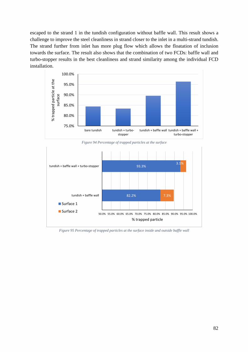
82
escaped to the strand 1 in the tundish configuration without baffle wall. This result shows a
challenge to improve the steel cleanliness in strand closer to the inlet in a multi-strand tundish.
The strand further from inlet has more plug flow which allows the floatation of inclusion
towards the surface. The result also shows that the combination of two FCDs: baffle wall and
turbo-stopper results in the best cleanliness and strand similarity among the individual FCD
installation.
Figure 94 Percentage of trapped particles at the surface
Figure 95 Percentage of trapped particles at the surface inside and outside baffle wall
75.0%
80.0%
85.0%
90.0%
95.0%
100.0%
bare tundish tundish + turbo-stopper
tundish + baffle wall tundish + baffle wall +turbo-stopper
% t
rap
ped
par
ticl
e at
th
e su
rfac
e
82.2%
93.3%
7.3%
3.1%
50.0% 55.0% 60.0% 65.0% 70.0% 75.0% 80.0% 85.0% 90.0% 95.0% 100.0%
tundish + baffle wall
tundish + baffle wall + turbo-stopper
% trapped particle
Surface 1
Surface 2
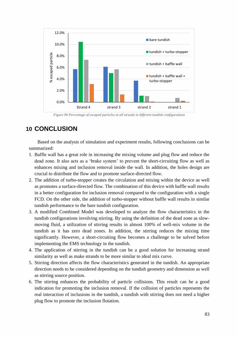
83
Figure 96 Percentage of escaped particles at all strands in different tundish configurations
10 CONCLUSION
Based on the analysis of simulation and experiment results, following conclusions can be
summarized:
1. Baffle wall has a great role in increasing the mixing volume and plug flow and reduce the
dead zone. It also acts as a ‘brake system’ to prevent the short-circuiting flow as well as
enhances mixing and inclusion removal inside the wall. In addition, the holes design are
crucial to distribute the flow and to promote surface-directed flow.
2. The addition of turbo-stopper creates the circulation and mixing within the device as well
as promotes a surface-directed flow. The combination of this device with baffle wall results
in a better configuration for inclusion removal compared to the configuration with a single
FCD. On the other side, the addition of turbo-stopper without baffle wall results in similar
tundish performance to the bare tundish configuration.
3. A modified Combined Model was developed to analyze the flow characteristics in the
tundish configurations involving stirring. By using the definition of the dead zone as slow-
moving fluid, a utilization of stirring results in almost 100% of well-mix volume in the
tundish as it has zero dead zones. In addition, the stirring reduces the mixing time
significantly. However, a short-circuiting flow becomes a challenge to be solved before
implementing the EMS technology in the tundish.
4. The application of stirring in the tundish can be a good solution for increasing strand
similarity as well as make strands to be more similar to ideal mix curve.
5. Stirring direction affects the flow characteristics generated in the tundish. An appropriate
direction needs to be considered depending on the tundish geometry and dimension as well
as stirring source position.
6. The stirring enhances the probability of particle collisions. This result can be a good
indication for promoting the inclusion removal. If the collision of particles represents the
real interaction of inclusions in the tundish, a tundish with stirring does not need a higher
plug flow to promote the inclusion flotation.
0.0%
2.0%
4.0%
6.0%
8.0%
10.0%
12.0%
Strand 4 strand 3 strand 2 strand 1
% e
scap
ed p
arti
cle
bare tundish
tundish + turbo-stopper
tundish + baffle wall
tundish + baffle wall +turbo-stopper

84
7. Care should be taken into consideration regarding the surface turbulence condition when
implement stirring in the tundish. Excessive stirring and inappropriate stirring direction may
generate high surface turbulence and a high backflow.
11 FURTHER STUDY
Considering some limitations in the results and analysis, following suggestion should be
conducted for further research:
1. A numerical simulation of pump stirring should be conducted to have more comprehensive
comparison regarding the effect of EMS and FCD on tundish performance.
2. A combination of stirring with other baffle wall design is necessary to find the best solution
to avoid short-circuiting flow in stirring configuration.
3. The ideal plug to well mix ratio in the tundish need to be investigated as this parameter can
be a reference to determine the best tundish configuration to solve problems in the multi-
strand tundish.
4. Modelling of inclusion removal in water model would be a beneficial experiment to have a
better understanding of inclusion removal from a physical model.

85
12 REFERENCES
[1] Yogeshwar Sahai, ”Tundish Technology for Casting Clean Steel : A review,”
Metallurgical and Materials Transactions B, vol. 47, nr 4, p. 2095–2106, 2016.
[2] A. Dewan and S. Gupta, "Comparison of Different Multi-Strand Tundishes,"
International Review of Mechanical Engineering, vol. 8, no. 1, 2014.
[3] S.-G. Zheng and M.-Y. Zhu, "Optimization of flow control devices in a ten-strand billet
caster tundish," China Foundry, vol. 13, pp. 414-421, 2016.
[4] J. Pieprzyca, Z. Kudlins and T. Merder, "Effect of Temperature Fields Heterogeneity in
the Tundish on Primary Structure of Continuously Cast Ingots," Metallurgy and Material,
vol. 60, no. I, 2015.
[5] S.-G. Zheng and M.-Y. Zhu, "Optimisation of baffles in six strand round bloom
continuous casting tundish : A physical modelling study," Ironmaking & Steelmaking,
vol. 33, no. 5, p. 398–406, 2013.
[6] T. Merder and M. Warzecha, "Optimization of a Six-Strand Continuous Casting Tundish
: Industrial Measurements and Numerical Investigation of the Tundish Modifications,"
Metallurgical and Materials Transactions B, vol. 43, no. 4, p. 856–868, 2012.
[7] C. M. Fan, S. M. Pan, H. S. Wang and W. S. Hwang, "Design of single element flow
control device in twin strand billet tundish for continuous casting of steel using flow,"
Ironmaking & Steelmaking, vol. 29, no. 5, pp. 376-382, 2013.
[8] P. K. Jha, S. Dash and S. Kumar, "Fluid Flow and Mixing in a Six Strand Billet Caster
Tundish: A Parametric Study," ISIJ Internationa, vol. 41, no. 12, pp. 1437-1446, 2001.
[9] "www.jfe-holdings.co.jp," Japan, [Online]. Available: http://www.jfe-
holdings.co.jp/en/investor/zaimu/ar/2005/tokusyu01.html. [Accessed 11 June 2018].
[10] [Online]. Available: http://www.designfax.net/cms/dfx/opens/article-view-
dfx.php?nid=4&bid=378&et=featurearticle&pn=01. [Accessed 11 June 2018].
[11] Y. Sahai and T. Emi, Tundish Technology for Clean Steel Production, World Scientific
Publishing Co. Pte. Ltd, 2008.
[12] L.Sowa, "Effect Of Steel Flow Control Devices On Flow And Temperature Field In The
Tundish," Archive of Metallurgy and Materials, vol. 60, no. 2, 2015.
[13] K. Badr, M. Tomas, M. Kirschen and G. McIlveney, "Refractory Solutions to Improve
Steel Cleanliness," RHI Bulletin, vol. I, pp. 43-50, 2011.
[14] B. G. Thomas, ”Continuous Casting Operation . Fluid Flow,” i Making, Shaping, and
Treating of Steel, 11th Ed, AISE Steel Found, 2000.
[15] Y. Sahai and T. Emi, "Criteria for Water Modeling of Melt Flow and Inclusion Removal
n Continuous Casting Tundishes," ISIJ International,, vol. 36, no. 9, pp. 1166-1173,
1996.
[16] J. H. Cloete, "Flow Analysis of a Four-strand Steelmaking Tundish Using Physical and
Numerical Modelling," Stellenbosch University, 2014.
[17] L.-c. Zhong, R.-c. Hao, J.-z. Li and Y.-x. Zhu, "Molten Steel Flow in a Slab Continuous-

86
casting Tundish," Journal of Iron and Steel Research, International, vol. 21, 2014.
[18] H. S. Fogler, "Distributions of Residence Times for Chemical Reactors," in Elements of
chemical reaction engineering, 4th edition, Upper Saddle River NJ, Prentice Hall PTR,
2006, p. 872.
[19] Y. Sahai and T. Emi, "Melt Flow Characterization in Continuous Casting Tundishes,"
ISIJ International, vol. 36, no. 6, pp. 667-672, 1996.
[20] A. Kumar, S. C. Koria and D. Mazumdar, "Basis for Systematic Hydrodynamic Analysis
of a Multi-strand Tundish," ISIJ International, vol. 47, no. 11, pp. 1618-1624, 2007.
[21] Ahuja and Sahai, "Steel Flow and Mixing of Melt in Steelmaking Tundishes,"
Ironmaking & Steelmaking, vol. 13, pp. 241-247, 1986.
[22] M. Bensouici, A. Bellaouar and K. Talbi, "Numerical Investigation of the Fluid Flow in
Continuous Casting Tundish Using Analysis of RTD Curves," Journal of Iron and Steel
Research International, vol. 16, no. 2, pp. 22-29, 2009.
[23] J. Cloete, G. Akdogan, S. Bradshaw and D. Chibwe, "Physical and numerical modelling
of a four-strand steelmaking tundish using flow analysis of different configurations,"
South African Institute of Mining and Metallurgy, vol. 11, pp. 355-362, 2015.
[24] J. K. a. J. Mastervich, "Proceedings of the 69th Steelmaking Conference," Washington
DC, I&S Society, 1986.
[25] J. Fan, Q. Zhang, Z. M. H. Lei and W. Wang, Iron Steel, vol. 33, pp. 24-28, 1998.
[26] S. Zheng, M. Zhu, G. Jiang and J. Song, Iorn Steel, vol. 39, pp. 23-25, 2004.
[27] K. Chattopadhyay, I. Mihaiela and R. I. Guthrie, "Physical and Mathematical Modelling
of SteelmakingTundish Operations: A Review of the Last Decade ( 1999- 2009)," ISIJ
International, vol. 50, no. 3, pp. 331-348, 2010.
[28] B. Bulko and J. Kijac, "Optimization of Tundish Equipment," Acta Metallurgica Slovaca,
vol. 16, no. 2, pp. 76-83, 2010.
[29] Z. Miaoyong, C. Nailiang and H. Yang, "http://millennium-steel.com," 2005. [Online].
Available: http://millennium-steel.com/wp-content/uploads/articles/pdf/2005/pp101-
104%20MS05.pdf. [Accessed 6 March 2018].
[30] [Online]. Available: https://www.comsol.com/multiphysics/navier-stokes-equations.
[Accessed 11 June 2018].
[31] A. Bakker. [Online]. Available: http://www.bakker.org/dartmouth06/engs150/15-
dpm.pdf. [Accessed 11 June 2018].
[32] ANSYS, "Modeling Turbulent FLows, Introductory FLuent Training," ANSYS, Inc,
2006.
[33] A. Fluent, "Introduction to Ansys Fluent 14.5, Lecture 7: Turbulence," Ansys, Inc, 2012.
[34] ”Modelling Of turbulent Flows, Introductory FLUENT training”.
[35] "ANSYS Fluent User Guide," [Online]. Available:
https://www.sharcnet.ca/Software/Fluent6/html/ug/node1067.htm. [Accessed 08 March
2018].
[36] A. Fluent, "Solver Settings, Introductory FLUENT Training," ANYS, Inc, 2006.

APPENDIX A
Numerical Scheme and Solver Setting in simulation
Simulation number
Experiment Configuration
(Case Number)
Solution Methods : Pressure-Velocity Coupling Under Relaxation Factors
Scheme Gradient Pressure Momentum Turbulence
Kinetic Energy
Turbulent Dissipation
Rate Pressure Density
Body Forces
Momentum
Turbulent Kinetic Energy
Turbulent Dissipatio
n Rate
Turbulent Viscosity
1 bare tundish(1) SIMPLEC Least
Squares Cell Based
Second Order
Second Order
Upwind
Second Order
Upwind
Second Order
Upwind 0.3 1 1 0.7 0.2 0.2 0.5
2 bare tundish(1) SIMPLEC Least
Squares Cell Based
Second Order
Second Order
Upwind
Second Order
Upwind
Second Order
Upwind 0.3 1 1 0.7 0.2 0.2 0.5
3 bare tundish(1) SIMPLEC Least
Squares Cell Based
Second Order
Second Order
Upwind
Second Order
Upwind
Second Order
Upwind 0.3 1 1 0.7 0.2 0.2 0.5
4 bare tundish(1) SIMPLEC Least
Squares Cell Based
Second Order
Second Order
Upwind
Second Order
Upwind
Second Order
Upwind 0.3 1 1 0.7 0.2 0.2 0.5
5 bare tundish(1) SIMPLEC Least
Squares Cell Based
Second Order
Second Order
Upwind
Second Order
Upwind
Second Order
Upwind 0.3 1 1 0.7 0.2 0.2 0.5
6 Tundish +
Turbo-stopper (5)
SIMPLEC Least
Squares Cell Based
Standard First Order
Upwind First Order
Upwind First Order
Upwind 0.3 1 1 0.1 0.2 0.2 0.5
7 Tundish +
Baffle wall (10) SIMPLEC
Least Squares
Cell Based Standard
First Order Upwind
First Order Upwind
First Order Upwind
0.3 1 1 0.7 0.2 0.2 0.5
8
Tundish + Turbo-stopper
+ baffle wall (12)
SIMPLEC Least
Squares Cell Based
Standard First Order
Upwind First Order
Upwind First Order
Upwind 0.3 1 1 0.1 0.2 0.2 0.5
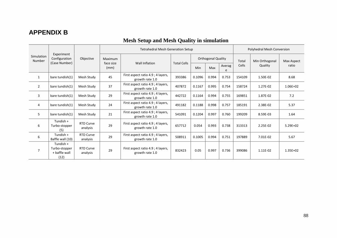
88
APPENDIX B
Mesh Setup and Mesh Quality in simulation
Simulation Number
Experiment Configuration
(Case Number) Objective
Tetrahedral Mesh Generation Setup Polyhedral Mesh Conversion
Maximum face size
(mm) Wall Inflation Total Cells
Orthogonal Quality Total Cells
Min Orthogonal Quality
Max Aspect ratio
Min Max Averag
e
1 bare tundish(1) Mesh Study 45 First aspect ratio 4.9 ; 4 layers,
growth rate 1.0 393386 0.1096 0.994 0.753 154109 1.50E-02 8.68
2 bare tundish(1) Mesh Study 37 First aspect ratio 4.9 ; 4 layers,
growth rate 1.0 407872 0.1167 0.995 0.754 158724 1.27E-02 1.06E+02
3 bare tundish(1) Mesh Study 29 First aspect ratio 4.9 ; 4 layers,
growth rate 1.0 442722 0.1164 0.994 0.755 169851 1.87E-02 7.2
4 bare tundish(1) Mesh Study 24 First aspect ratio 4.9 ; 4 layers,
growth rate 1.0 491182 0.1188 0.998 0.757 185191 2.38E-02 5.37
5 bare tundish(1) Mesh Study 21 First aspect ratio 4.9 ; 4 layers,
growth rate 1.0 541091 0.1204 0.997 0.760 199209 8.59E-03 1.64
6 Tundish +
Turbo-stopper (5)
RTD Curve analysis
29 First aspect ratio 4.9 ; 4 layers,
growth rate 1.0 657712 0.054 0.993 0.738 313313 2.25E-02 5.29E+02
6 Tundish +
Baffle wall (10) RTD Curve
analysis 29
First aspect ratio 4.9 ; 4 layers, growth rate 1.0
508911 0.1005 0.994 0.751 197889 7.01E-02 5.67
7
Tundish + Turbo-stopper
+ baffle wall (12)
RTD Curve analysis
29 First aspect ratio 4.9 ; 4 layers,
growth rate 1.0 832423 0.05 0.997 0.736 399086 1.11E-02 1.35E+02

APPENDIX C
• Velocity Mapping with stirring (30% pump capacity)
• Velocity Mapping with stirring (40% pump capacity)

90
APPENDIX D
Flow Behavior Observation
• Case 10: Tundish with baffle wall

91
APPENDIX E
Residence Time Distribution Curve from Experiment
• Case 5: Tundish + turbo-stopper
• Case 12: Tundish + baffle wall + turbo-stopper
0.0
0.5
1.0
1.5
2.0
2.5
3.0
0.0
0.2
0.4
0.5
0.7
0.9
1.1
1.3
1.4
1.6
1.8
2.0
2.2
2.3
2.5
2.7
2.9
3.1
3.2
3.4
3.6
3.8
4.0
Dim
ensi
on
less
Co
nce
ntr
atio
n
Dimensionless time
Strand 4 Strand 3 Strand 2 Strand 1
0
0.1
0.2
0.3
0.4
0.5
0.6
0.7
0.8
0.9
0.0
0.2
0.3
0.5
0.6
0.8
1.0
1.1
1.3
1.4
1.6
1.8
1.9
2.1
2.2
2.4
2.5
2.7
2.9
3.0
3.2
3.3
3.5
3.7
3.8
4.0
Dim
ensi
on
less
Co
nce
ntr
atio
n
Dimensionless time
Strand 4 Strand 3 Strand 2 Strand 1
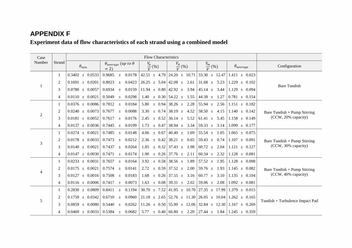
APPENDIX F
Experiment data of flow characteristics of each strand using a combined model
Case
Number
Strand
Flow Characteristics
𝜃𝑚𝑖𝑛 𝜃𝑎𝑣𝑒𝑟𝑎𝑔𝑒 (𝑢𝑝 𝑡𝑜 𝜃
= 2)
𝑉𝑝
𝑉(%)
𝑉𝑑
𝑉(%)
𝑉𝑚
𝑉(%) 𝜃𝑎𝑣𝑒𝑟𝑎𝑔𝑒 Configuration
1
1 0.3402 ± 0.0533 0.9685 ± 0.0178 42.51 ± 4.79 24.20 ± 10.71 33.30 ± 12.47 1.411 ± 0.023
Bare Tundish 2 0.1691 ± 0.0201 0.8023 ± 0.0423 26.25 ± 5.04 42.08 ± 2.61 31.68 ± 5.23 1.229 ± 0.102
3 0.0780 ± 0.0057 0.6934 ± 0.0159 11.94 ± 0.80 42.92 ± 3.94 45.14 ± 3.44 1.129 ± 0.094
4 0.0110 ± 0.0021 0.5049 ± 0.0298 1.40 ± 0.30 54.22 ± 1.55 44.38 ± 1.27 0.781 ± 0.154
2
1 0.0376 ± 0.0086 0.7812 ± 0.0184 5.80 ± 0.94 38.26 ± 2.28 55.94 ± 2.56 1.151 ± 0.182
Bare Tundish + Pump Stirring
(CCW, 20% capacity)
2 0.0240 ± 0.0073 0.7677 ± 0.0088 3.30 ± 0.74 38.19 ± 4.52 58.50 ± 4.15 1.140 ± 0.142
3 0.0181 ± 0.0052 0.7617 ± 0.0176 2.45 ± 0.52 36.14 ± 5.52 61.41 ± 5.45 1.158 ± 0.149
4 0.0137 ± 0.0036 0.7445 ± 0.0199 1.73 ± 0.47 38.94 ± 3.34 59.33 ± 3.14 1.099 ± 0.177
3
1 0.0274 ± 0.0021 0.7485 ± 0.0148 4.06 ± 0.67 40.40 ± 1.69 55.54 ± 1.05 1.065 ± 0.075
Bare Tundish + Pump Stirring
(CCW, 30% capacity)
2 0.0178 ± 0.0033 0.7473 ± 0.0212 2.36 ± 0.42 38.21 ± 0.65 59.43 ± 0.74 1.107 ± 0.091
3 0.0140 ± 0.0021 0.7437 ± 0.0264 1.85 ± 0.32 37.43 ± 1.98 60.72 ± 2.04 1.121 ± 0.127
4 0.0147 ± 0.0030 0.7471 ± 0.0174 1.90 ± 0.26 37.76 ± 2.11 60.34 ± 2.32 1.128 ± 0.081
4
1 0.0233 ± 0.0031 0.7657 ± 0.0164 3.92 ± 0.58 38.56 ± 1.89 57.52 ± 1.95 1.128 ± 0.098
Bare Tundish + Pump Stirring
(CCW, 40% capacity)
2 0.0175 ± 0.0021 0.7574 ± 0.0141 2.72 ± 0.59 37.52 ± 2.00 59.76 ± 1.93 1.145 ± 0.082
3 0.0127 ± 0.0016 0.7508 ± 0.0183 1.68 ± 0.26 37.55 ± 3.16 60.77 ± 3.10 1.135 ± 0.104
4 0.0116 ± 0.0006 0.7417 ± 0.0073 1.63 ± 0.08 39.31 ± 2.02 59.06 ± 2.08 1.092 ± 0.081
5
1 0.2830 ± 0.0809 0.8411 ± 0.1194 30.70 ± 7.52 41.95 ± 10.70 27.35 ± 17.99 1.379 ± 0.015
Tundish + Turbulence Impact Pad 2 0.1759 ± 0.0342 0.6710 ± 0.0960 21.18 ± 2.65 52.76 ± 11.30 26.05 ± 10.04 1.262 ± 0.165
3 0.0859 ± 0.0080 0.5440 ± 0.0262 11.26 ± 0.50 55.90 ± 12.06 32.84 ± 12.30 1.167 ± 0.269
4 0.0469 ± 0.0033 0.5384 ± 0.0682 5.77 ± 0.40 66.80 ± 2.20 27.44 ± 1.84 1.245 ± 0.359

93
APPENDIX F
Experiment data of flow characteristics of each strand using a combined model
Case
Number Strand
Flow Characteristics
𝜃𝑚𝑖𝑛 𝜃𝑎𝑣𝑒𝑟𝑎𝑔𝑒 (𝑢𝑝 𝑡𝑜 𝜃
= 2)
𝑉𝑑𝑝
𝑉(%)
𝑉𝑑
𝑉(%)
𝑉𝑚
𝑉(%) 𝜃𝑎𝑣𝑒𝑟𝑎𝑔𝑒 Configuration
6
1 0.0353 ± 0.0039 0.7621 ± 0.0258 4.66 ± 0.98 37.89 ± 1.32 57.45 ± 1.99 1.018 ± 0.147
Tundish + Turbulence Impact Pad
+ Pump Stirring (CCW, 20%
capacity)
2 0.0257 ± 0.0011 0.7538 ± 0.0314 3.87 ± 0.25 37.47 ± 2.47 58.66 ± 2.46 1.024 ± 0.170
3 0.0192 ± 0.0016 0.7563 ± 0.0208 2.91 ± 0.19 34.86 ± 1.21 62.23 ± 1.40 1.055 ± 0.158
4 0.0147 ± 0.0032 0.7443 ± 0.0202 1.95 ± 0.23 37.63 ± 1.57 60.41 ± 1.39 0.999 ± 0.126
7
1 0.0301 ± 0.0012 0.7843 ± 0.0220 4.19 ± 0.70 32.37 ± 4.43 63.44 ± 4.24 1.067 ± 0.167
Tundish + Turbulence Impact Pad
+ Pump Stirring (CCW, 30%
capacity)
2 0.0236 ± 0.0010 0.7746 ± 0.0303 3.95 ± 0.09 34.78 ± 2.93 61.27 ± 2.98 1.049 ± 0.192
3 0.0198 ± 0.0006 0.7699 ± 0.0221 3.18 ± 0.14 34.68 ± 4.40 62.13 ± 4.36 1.046 ± 0.158
4 0.0151 ± 0.0033 0.7571 ± 0.0209 2.21 ± 0.54 36.27 ± 3.56 61.53 ± 3.33 1.020 ± 0.162
8
1 0.0226 ± 0.0010 0.7684 ± 0.0059 4.11 ± 0.64 41.15 ± 0.97 54.74 ± 0.72 1.279 ± 0.048
Tundish + Turbulence Impact Pad
+ Pump Stirring (CCW, 40%
capacity)
2 0.0175 ± 0.0027 0.7578 ± 0.0175 3.20 ± 0.85 42.79 ± 0.78 54.01 ± 1.06 1.247 ± 0.070
3 0.0151 ± 0.0016 0.7520 ± 0.0075 2.34 ± 0.26 42.11 ± 1.52 55.55 ± 1.70 1.257 ± 0.035
4 0.0113 ± 0.0010 0.7462 ± 0.0030 1.64 ± 0.22 42.33 ± 1.76 56.03 ± 1.79 1.246 ± 0.032
9
1 0.0332 ± 0.0016 0.7932 ± 0.0279 11.36 ± 1.5412 33.53 ± 5.3711 55.11 ± 6.6905 1.144 ± 0.186
Bare tundish + Pump Stirring
(CW,20% capacity)
2 0.0352 ± 0.0036 0.8000 ± 0.0271 11.21 ± 1.3672 33.65 ± 2.8581 55.15 ± 4.2032 1.185 ± 0.166
3 0.0298 ± 0.0027 0.7879 ± 0.0255 7.51 ± 3.8676 34.68 ± 0.7022 57.81 ± 3.4188 1.172 ± 0.195
4 0.0128 ± 0.0007 0.6909 ± 0.0466 2.70 ± 1.0142 42.18 ± 3.2236 55.12 ± 4.1494 1.040 ± 0.195
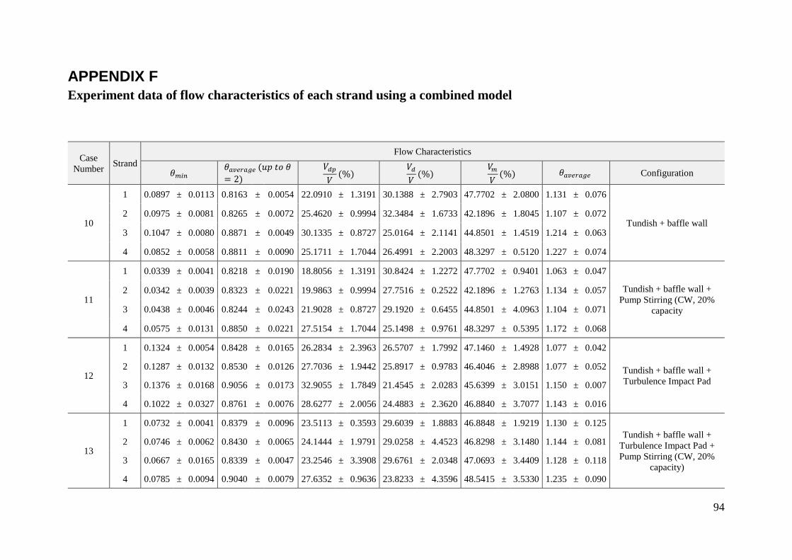
94
APPENDIX F
Experiment data of flow characteristics of each strand using a combined model
Case
Number Strand
Flow Characteristics
𝜃𝑚𝑖𝑛 𝜃𝑎𝑣𝑒𝑟𝑎𝑔𝑒 (𝑢𝑝 𝑡𝑜 𝜃
= 2)
𝑉𝑑𝑝
𝑉(%)
𝑉𝑑
𝑉(%)
𝑉𝑚
𝑉(%) 𝜃𝑎𝑣𝑒𝑟𝑎𝑔𝑒 Configuration
10
1 0.0897 ± 0.0113 0.8163 ± 0.0054 22.0910 ± 1.3191 30.1388 ± 2.7903 47.7702 ± 2.0800 1.131 ± 0.076
Tundish + baffle wall 2 0.0975 ± 0.0081 0.8265 ± 0.0072 25.4620 ± 0.9994 32.3484 ± 1.6733 42.1896 ± 1.8045 1.107 ± 0.072
3 0.1047 ± 0.0080 0.8871 ± 0.0049 30.1335 ± 0.8727 25.0164 ± 2.1141 44.8501 ± 1.4519 1.214 ± 0.063
4 0.0852 ± 0.0058 0.8811 ± 0.0090 25.1711 ± 1.7044 26.4991 ± 2.2003 48.3297 ± 0.5120 1.227 ± 0.074
11
1 0.0339 ± 0.0041 0.8218 ± 0.0190 18.8056 ± 1.3191 30.8424 ± 1.2272 47.7702 ± 0.9401 1.063 ± 0.047
Tundish + baffle wall +
Pump Stirring (CW, 20%
capacity
2 0.0342 ± 0.0039 0.8323 ± 0.0221 19.9863 ± 0.9994 27.7516 ± 0.2522 42.1896 ± 1.2763 1.134 ± 0.057
3 0.0438 ± 0.0046 0.8244 ± 0.0243 21.9028 ± 0.8727 29.1920 ± 0.6455 44.8501 ± 4.0963 1.104 ± 0.071
4 0.0575 ± 0.0131 0.8850 ± 0.0221 27.5154 ± 1.7044 25.1498 ± 0.9761 48.3297 ± 0.5395 1.172 ± 0.068
12
1 0.1324 ± 0.0054 0.8428 ± 0.0165 26.2834 ± 2.3963 26.5707 ± 1.7992 47.1460 ± 1.4928 1.077 ± 0.042
Tundish + baffle wall +
Turbulence Impact Pad
2 0.1287 ± 0.0132 0.8530 ± 0.0126 27.7036 ± 1.9442 25.8917 ± 0.9783 46.4046 ± 2.8988 1.077 ± 0.052
3 0.1376 ± 0.0168 0.9056 ± 0.0173 32.9055 ± 1.7849 21.4545 ± 2.0283 45.6399 ± 3.0151 1.150 ± 0.007
4 0.1022 ± 0.0327 0.8761 ± 0.0076 28.6277 ± 2.0056 24.4883 ± 2.3620 46.8840 ± 3.7077 1.143 ± 0.016
13
1 0.0732 ± 0.0041 0.8379 ± 0.0096 23.5113 ± 0.3593 29.6039 ± 1.8883 46.8848 ± 1.9219 1.130 ± 0.125
Tundish + baffle wall +
Turbulence Impact Pad +
Pump Stirring (CW, 20%
capacity)
2 0.0746 ± 0.0062 0.8430 ± 0.0065 24.1444 ± 1.9791 29.0258 ± 4.4523 46.8298 ± 3.1480 1.144 ± 0.081
3 0.0667 ± 0.0165 0.8339 ± 0.0047 23.2546 ± 3.3908 29.6761 ± 2.0348 47.0693 ± 3.4409 1.128 ± 0.118
4 0.0785 ± 0.0094 0.9040 ± 0.0079 27.6352 ± 0.9636 23.8233 ± 4.3596 48.5415 ± 3.5330 1.235 ± 0.090
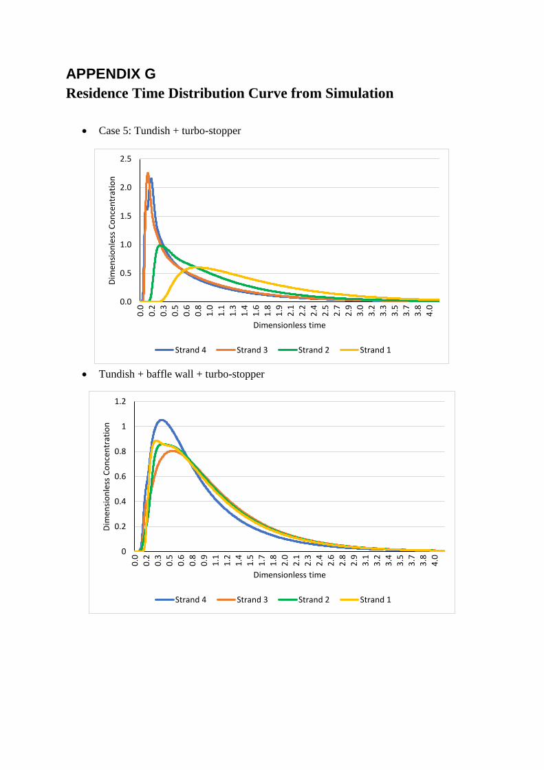
APPENDIX G
Residence Time Distribution Curve from Simulation
• Case 5: Tundish + turbo-stopper
• Tundish + baffle wall + turbo-stopper
0.0
0.5
1.0
1.5
2.0
2.5
0.0
0.2
0.3
0.5
0.6
0.8
1.0
1.1
1.3
1.4
1.6
1.8
1.9
2.1
2.2
2.4
2.5
2.7
2.9
3.0
3.2
3.3
3.5
3.7
3.8
4.0
Dim
ensi
on
less
Co
nce
ntr
atio
n
Dimensionless time
Strand 4 Strand 3 Strand 2 Strand 1
0
0.2
0.4
0.6
0.8
1
1.2
0.0
0.2
0.3
0.5
0.6
0.8
0.9
1.1
1.2
1.4
1.5
1.7
1.8
2.0
2.1
2.3
2.4
2.6
2.8
2.9
3.1
3.2
3.4
3.5
3.7
3.8
4.0
Dim
ensi
on
less
Co
nce
ntr
atio
n
Dimensionless time
Strand 4 Strand 3 Strand 2 Strand 1

APPENDIX H
Simulation data of flow characteristics of each strand using a combined model
Case Number Strand
𝜃𝑚𝑖𝑛 𝜃𝑎𝑣𝑒𝑟𝑎𝑔𝑒 (𝑢𝑝 𝑡𝑜 𝜃 = 2) 𝑉𝑑𝑝
𝑉(%)
𝑉𝑑
𝑉(%)
𝑉𝑚
𝑉(%)
𝑉𝑝
𝑉𝑑
Configuration
1
1 0.1324 1.2564 63.76 15.19 21.05 4.197
Bare Tundish 2 0.0257 0.7603 7.91 31.97 60.13 0.247
3 0.0113 0.5682 4.11 46.53 49.36 0.088
4 0.0092 0.5203 2.00 50.67 47.33 0.040
5
1 0.0893 1.1199 43.58 17.08 39.33 2.551
Tundish + Turbulence Impact Pad 2 0.0298 0.8223 15.25 27.32 57.44 0.558
3 0.0133 0.5947 6.11 44.59 49.30 0.137
4 0.0103 0.5548 8.11 47.63 44.26 0.170
10
1 0.0185 0.8590 23.9733 22.4977 53.5290 1.0656
Tundish + baffle wall 2 0.0164 0.8689 24.7433 21.7624 53.4943 1.1370
3 0.0144 0.8824 28.6961 21.1501 50.1538 1.3568
4 0.0123 0.7510 16.7351 30.4412 52.8237 0.5498
12
1 0.0277 0.8194 15.8111 25.1050 59.0839 0.6298
Tundish + baffle wall + Turbulence Impact Pad 2 0.0164 0.8401 19.4045 23.4817 57.1138 0.8264
3 0.0133 0.8542 25.7700 22.6310 51.5990 1.1387
4 0.0123 0.7417 18.7372 30.6461 50.6167 0.6114

www.kth.se