The Effect of Different Potentials for

Paul Traps and it’s Application as a Quan-

tum Simulator

Bachelor Thesis

Skrevet af Anton L. AndersenMarch 28, 2018

Under vejledning af

Anders Søndberg Sørensen

Københavns Universitet

Formal Data

Name: Anton L. AndersenEmail: wpl223@alumni.ku.dk

University of CopenhagenFaculty of ScienceNiels Borh Instituttet

Hand in date: 28.03.2018

Abstract

In this project we will consider the capabilities of a linear ion trap as a QuantumSimulator. The project considers di↵erent choices for potentials along the trap andexamines how the di↵erent potentials a↵ect the spacing of the ions held in place.Modes of transversal oscillations of the ions are found and used as a basis for theimplementation of the Mølmer–Sørensen gate. Coupling strength between the ionsare found from numerical evaluation.The proposed changes to the potentials seems to be an improvement over the har-monic potential, especially with detuning of � ⇠ 1.2!COM where behaves like adipole-dipole interaction. For detuning close to the center of mass motion � ⇠ !COM

the coupling strength will be constant across the ion chain and long range spin-spininteraction can occur.

2

Contents

1 Introduction 4

2 Linear Ion Trap 4

2.1 Choice of Trap Potential . . . . . . . . . . . . . . . . . . . . . . . . . 5

2.2 Longitudinal Oscillations . . . . . . . . . . . . . . . . . . . . . . . . . 7

2.3 Transversal Oscillations . . . . . . . . . . . . . . . . . . . . . . . . . . 8

2.4 Zigzag Configuration of the Ions . . . . . . . . . . . . . . . . . . . . . 9

3 Quantum Mechanics 11

3.1 Ion-Laser Interaction . . . . . . . . . . . . . . . . . . . . . . . . . . . 12

3.2 Perturbative Treatment of the Transitions . . . . . . . . . . . . . . . 13

3.3 Evaluating the Rabi frequency . . . . . . . . . . . . . . . . . . . . . . 15

4 Numerical Analysis 17

5 Possible Improvements 19

6 Conclusion 20

3

1 Introduction

A model of great importance in many areas of physics is the Ising Model, whichin it’s general form is described by the hamiltonian H = �

PJij�i�j � µ

Phj�j.

Models like this forms a basis for our understanding of ferromagnets. To calculatespin coupling for N ions in a lattice one needs to consider 2N di↵erent spin states,which quickly becomes to big of a problem to handle with classical computers. Feyn-man stipulated the idea of a quantum simulator, which makes use of the quantummechanical nature of the computer itself to solve problems[1]. One method whichhas enjoyed succes in recent years is the idea of using a ion trap as a quantum sim-ulator, in which a number of ions are held in place by an electric potential and thencontrolled by a laser. With this setup it has been possible to confine and control upto N = 53 ions in a linear trap paul-trap[2] and N ⇠ 300 ions in a two-dimensionalpenning trap[3].

2 Linear Ion Trap

Consider a chain of N ions held in place by an electric potential Vtrap along thedirection of the chain. Let R1(t),R2(t), . . . ,RN(t) denote the position of the ionsin a coordinate system placed such that the ions are placed along the z-axis. Wemay number the ions such that zm < zm+1 for m = 1, . . . , N � 1. The ions areheld in place radially by a rapidly oscillating electrical field, which we’ll assume fornow is so strong that xm = ym = 0 for all ions. Along with the potential the ionsalso interact with each other through coulomb interaction. Therefore the potentialenergy of the chain is,

V =NX

m=1

Vtrap(zm) +NX

n,m=1n 6=m

Z2e2

8⇡"0

1

|zn � zm|, (1)

where Z is the degree of ionisation of the ions, e is the elementary charge and "0 isthe vacuum permittivity. The equilibrium positions z01 , z

02 , . . . , z

0N

are given by thesolutions to the N coupled equations

@V

@zm

�

0

= 0, m = 1, . . . , N, (2)

where the notation [ · ]0 means that the term is to be evaluated at zm = z0mfor all

m. These equations are dependant on the choice of trap potential Vtrap, and willgenerally be too complicated to solve analytically. If the trap potential is chosen to

4

be harmonic Vtrap(z) =12M⌫

2z2 where M is the mass of the ion, it will be possible

to solve the system analytically for N = 2 and N = 3[4], but generally one have torely on numerical methods to find the equilibrium positions.

2.1 Choice of Trap Potential

It is generally desirable for the ions in the trap to be equidistance, as it will greatlysimplify any models that seek to describe the interaction between the ions. Anotherwish is for the trap potential to be simple, as that would make it easier to constructand work with experimentally. These two wishes can’t be achieved at the sametimes and thus a compromise between the two is needed.

A harmonic potential is an obvious choice to satisfy these criteria. This is also thepotential used in many experiments [2]. This potential has the advantages of beingeasy to work with both theoretically and experimentally, however it su↵ers fromthe fact that the ions are equidistance. To counter this one could change the trappotential used. This thesis examines four di↵erent choices of potential,

• V(2)trap(z) =

12M⌫

2z2

• V(4)trap(z) =

�44l2M⌫

2z4

• V(6)trap(z) =

�66l4M⌫

2z6

• V(8)trap(z) =

�88l6M⌫

2z8

where the scale length l is defined by,

l3 =

Z2e2

4⇡"0M⌫2, (3)

and �4,�6 and �8 allows us to tune the strength of the potentials such that thelength of the ion chain remains the same no matter the choice of potential. Theequilibrium positions for these potentials are found by solving (2) numerically. Todetermine �i for the di↵erent potentials, a method was used where the equilibriumpositions were found with �i = 1. This produced a set of coordinates z01, z

02, . . . , z

0N

for each potential, these were scaled to be the same length as the chain producedby V

(2)trap. The scaled coordinates were then plugged back into (2), which this time

were solved for �i. Then to double check the result (2) were used with the newlyfound �i to ensure that the coordinates matched the scaled coordinates. This was

5

done for chains consisting from 4 to 100 ions.

We can now compare how the ions are spaced for the di↵erent potentials. One wayto do this is to find the standard deviation � for the distance between neighbouringions

� =

vuut 1

N � 1

N�1X

i=1

(di � d) (4)

where di = (z0i+1 � z

0i)/l is the spacing between neighbouring ions in units of the

scale length l and d is the mean spacing. A plot with � for the di↵erent potentialsfor 4 N 100 is found in figure 1. From it we can see that the proposed potentialsV

(4)trap,V

(6)trap and V

(8)trap are significantly better at separating the ions with equal distance

than the harmonic potential V (2)trap when theres more than 10 ions in the chain.

Figure 1: The standard deviation of the distance between neighbouring ions in unitsof the scale length l as defined in (3). This makes it possible to determine the regimein which the di↵erent potentials will the give the most uniform distribution of theions. For N = 4 V

(2)trap is the best choice, for 5 N < 12 it is V (4)

trap, for 12 N < 22

it is V (6)trap and for 22 N it is V (8)

trap.

6

2.2 Longitudinal Oscillations

We now wish to consider the motion of the ions. Let zm(t) = z0m+ qm(t) such

that qm(t) describes the displacement of the ions compared to the equilibrium as afunction of time. The Lagrangian corresponding to this motion is

L =1

2

NX

m=1

q2mM � 1

2

NX

m,n=1

qnqm

@2V

@qn@qm

�

0

(5)

where dot notation is used to denote the time derivative and terms of order q3 andhigher have been omitted. Defining fk = �k(k�1)uk�2

mand letting the trap potential

be V(trapk), allows the Lagrangian to be rewritten as

L =M

2

"NX

m=1

q2m� ⌫

2NX

m,n=1

qnqmAnm

#, (6)

where

Anm =

(fk + 2

PN

i=11

|um�ui|3 , if n = m,

� 1|un�um|3 , if n 6= m.

(7)

The matrix A with as it’s entries is real, symmetric and positive semidefinite[4] so itseigenvalues must be non-negative. Number the eigenvalues µp and correspondingeigenvectors b

(p), p = 1, . . . , N , such that µ1 have the lowest eigenvalue, µ2 the

second lowest and so on. We may assume that the eigenvectors are normalised

NX

p=1

b(p)nb(p)m

= �nm,

NX

m=1

b(p)mb(q)m

= �pq (8)

where b(p)m is the m

th entry of the pth eigenvector. Define the normal modes as

Qp =X

m

b(p)mqm, (9)

then

qm =X

p

b(p)mQp. (10)

By defining the angular frequency of the pth mode as ⌫p =pµp⌫, allows us to write

the Lagrangian as

L =M

2

NX

p=1

hQ

2p� ⌫

2pQ

2p

i(11)

7

The canonical momentum is Pp = MQp and thus allows the hamiltonian to beexplicitly written

H =X

p

1

2MP

2p+

M

2⌫2pQ

2p

�. (12)

2.3 Transversal Oscillations

Let’s now consider transversal ocsillations. The ion trap is set up in the same wayas before with the N ions along the z direction. Along the z-direction the ions arestill held in place by the four di↵erent trap potentials. Along the x- and y-axis theions are held in place by a rapidly oscillating electrical field which to the secondorder may be approximated by the e↵ective radial potential,

Vrad =1

2M⌫

2rad

(x2m+ y

2m). (13)

This potential will be added to eq.(1) along with a change from |zn�zm| to |Rn�Rm|in the coulomb part to reflect that the ions now di↵er in the radial coordinate aswell,

V =NX

m=1

✓Vtrap(zm) +

1

2M⌫

2rad

(x2m+ y

2m)

◆+

NX

n,m=1n 6=m

Z2e2

8⇡"0

1

|Rn �Rm|. (14)

Suppose the ions all oscillate along the x-direction. The Lagrangian that describesthis motion is analogue to the longitudinal case

L =1

2

NX

m=1

x2mM �

NX

m,n=1

xnxm

@2V

@xn@xm

�

0

!(15)

Carrying out the di↵erentiation and evaluating at equilibrium position yields

@2V

@xn@xm

�

0

=

8<

:M⌫

2rad

� Z2e2

4⇡"0

PN

i=1i 6=n

1|zi�zn|3 , if n = m,

Z2e2

4⇡"01

|zn�zm|3 , if n 6= m.

(16)

Define the ratio between the radial potential strength and the strength of the har-monic trap potential as � = ⌫

⌫rad, such that the Lagrangian becomes

L =M

2

"NX

m=1

x2m� ⌫

2rad

NX

m,n=1

xnxmBnm

#(17)

8

where

Anm =

8<

:1� �

2P

N

i=1i 6=n

1|um�ui|3 , if n = m,

�2 1|un�um|3 , if n 6= m.

(18)

Just like before we can find eigenvalues ⇢p and eigenvectors 'p for B, and like beforethe Lagrangian can be written in terms of the modes defined by �p =

Pm'm,pxm

and the angular frequency of the modes !p =p⇢p⌫rad. Thus

L =M

2

NX

p=1

h�2

p� !

2p�2

p

i. (19)

However this time the eigenvalues could be negative. In the limit � ! 1 the matrixB will be negative definite, which will result in negative eigenvalues and imaginaryfrequencies. This reflects that the radial potential is not strong enough to keepthe lowest energy configuration of the ions to be a linear configuration. The lowestenergy configuration will instead be a zigzag or helical configuration.

2.4 Zigzag Configuration of the Ions

In order to avoid a zigzag configuration of the ions in the trap, the strength ofthe trap potential compared to the radial potential must be weak enough to avoidthe lowest energy configuration of the ions to be a zigzag configuration. Start byconsidering the potential of the ion chain as described in equation (14)

V =1

2M!

2rl2

2

664NX

m=1

⇣Vz(zm) + r

2m

⌘+

NX

n,m=1n 6=m

1

|Rn � Rm|

3

775 (20)

where the positions of the ions are described by the scaled cylindrical set of coordin-ates Rm(rm, ✓m, zm). The lowest energy configuration of this potential is either alinear, a zigzag or a helical configuration [5]. Because of the symmetry of the trapthe linear configuration where r1 = · · · = rN = 0 will always be at equilibrium. Itwill however not always be stable, if Vz is too strong a small perturbation such as alaser pulse will cause the ions to decay into a lower zigzag configuration. The linearconfiguration is stable if @

2V

@r2m> 0, which is equivalent to

@2

@r2m

2

664NX

m=1

⇣Vz(zm) + r

2m

⌘+

NX

n,m=1n 6=m

1

|Rn � Rm|

3

775 > 0 (21)

9

Carrying out the di↵erentiation and evaluating in the linear configuration yields therather pleasing

2�NX

n=1n 6=m

1

|⇣nm|3> 0 (22)

where ⇣nm = |rn � rm|. In practice it is only necessary to evaluate this expressionfor m ⇡ N/2 as this is the area with the least seperation between the ions. Thisequation relates the raidal potential trough the scale length l to the trap potentialthrough the set of zm. This along with the way of finding zm as described in a pre-vious section provides a way, although indirectly, to gauge the choices of potentialstrengths.For the rest of the thesis we’ll treat the transversal case as it produces signific-antly better results and it is the way the experiments are done today [6][2]. Thelongitudinal case follows analogously.

10

3 Quantum Mechanics

Now let’s consider the system quantum mechanically. Given the classical hamilto-nian of the system

H =1

2M

NX

p=1

P2p+

M

2

NX

p=1

!2p�2

p(23)

Introduce the ladder-operators a†pand ap which raises and lowers the respective

phonon mode and obeys the canonical commutation relations

[ai, aq] = 0, [a†q, a

†q] = 0, [ap, a

†q] = �qp. (24)

Make the substitution

�p ! �p =

s~

2M!p

(a†p+ ap) (25)

Pp ! Pp = i

r~M!p

2(a†

p� ap) (26)

(27)

which yields

H =1

2M

NX

p=1

i

r~M!p

2(a†

p� ap)

!2

+M

2

NX

p=1

!2p

s~

2M!p

(a†p+ ap)

!2

(28)

=X

p

!p~✓a†pap +

1

2

◆(29)

which is the hamiltonian corresponding to the quantum motion of the ions. This isaccompanied by an internal hamiltonian

H = ~!eg

NX

i=1

�zi

2(30)

where ~!eg is the energy di↵erence between the internal energy levels of a single ionand �zi is the Pauli matrix corresponding to the i’th ion in the chain. Combinedthese two yields the complete time independant part of the full hamiltonian

H0 =X

p

!p~✓a†pap +

1

2

◆+ ~!eg

NX

i=1

�zi

2(31)

with the set of eigenstates {|f1, f2, . . . , fN , n1, . . . , nNi} where fi = e or g and np isthe excitation of the p

th vibrational mode.

11

3.1 Ion-Laser Interaction

We can now turn our attention to the interaction between the laser and the ions.Consider the system consisting of a single ion which obeys the single ion version ofeq. (31),

H0 = ~⌫✓a†a+

1

2

◆+ ~!eg

�z

2. (32)

Suppose the system is exposed to a monochromatic electromagnetic plane-wave,described by the E-field,

E(r, t) = E0ei(k·r�!t) + E0e

�i(k·r�!t) (33)

where k is the wave vector and is chosen such that the wave propagates in the x-direction. We assume that the internal energy levels couple through the electricalfield, so we may write the hamiltonian for this interaction as [7]

H1 = �µd ·E(r, t), (34)

where µd is the electric dipole moment operator. This can be written as

H1 =~⌦2(�+ + ��)

�ei(k·r�!t) + e

�i(k·r�!t)�

(35)

where ⌦ is the Rabi frequency of the transition and is given by ~⌦ = �|µd|E0/2 and�± = �x ± i�y are the Pauli matrices relating to the internal energy levels. We’llnow transition to the interaction picture by the transformation U = e

i!egt|eihe| whichwe’ll expand in a series and utillize that |ei and |gi form an orthonormal basis so atheorem from linear algebra yields |ei he|+ |gi hg| = 1

U = 1 + i!egt |ei he|+1

2(i!egt)

2 |ei he|+ · · · (36)

= |gi hg|+ |ei he|+ i!egt |ei he|+1

2(i!egt)

2 |ei he|+ · · · (37)

Collecting the terms with |ei he| and substituting the terms which depends on |ei he|with an exponential yields,

U = |gi hg|+ ei!egt |ei he| (38)

(39)

We use this to transform H1 into the interaction picture,

H1,I = UH1U† = ~⌦

⇥�e�i(k·r�(!+!eg)t) + e

i(k·r�(!�!eg)t)�|ei hg|+ h.c.

⇤(40)

12

where h.c. is the Hermitian conjugate. We chose a detuning such that the energyof the laser is close to that of the internal energy di↵erence. This means that!�!eg ⌧ !+!eg and we may neglect the terms involving !+!eg because they arerapidly oscillating and thus will average to 0 on any applicable time scale. Usingthis approximation which is called a rotating wave approximation and transformingback to the Schrodinger picture gives us,

H1 = U†H1,IU =

~⌦2

��+e

i(k·r�!t) + h.c.�. (41)

The generalisation to the chain of N ions is straightforward

H1 =X

i

~⌦i

2

��+ie

i(ki·ri�!it) + h.c.�

(42)

where the sum is over all ions a↵ected by a laser. We have the freedom to let di↵erentlasers with di↵erent strength and frequency address the di↵erent ions. The last thingwe’ll do is to consider the term (k · r) in the exponent. The wave propagates in thex-direction and thus k = kx. Recall x-coordinate of the ion is described through thetransversal modes of oscillation, �p, by xm =

Pp'm,p�p and the modes are given

by eq. (25). This allows us to write

km · rm =X

p

km�m,p

s~

2M!p

(a†p+ ap). (43)

Define the Lamb-Dicke parameter as,

⌘m,p = km�m,p

s~

2M!p

, (44)

such that we may write the hamiltonian as

H1 =X

i

~⌦i

2

⇣�+ie

i[P

p ⌘i,p(a†p+ap)�!it] + h.c.

⌘, (45)

which will, along with eq. (31), form the basis of out further analysis.

3.2 Perturbative Treatment of the Transitions

We’ll let the laser be bichromatic with the two angular frequencies !1 = ! � � and!2 = ! + �. The way the vibrational modes are laid out means that the detuning �

is chosen to over/undershoot the first excitation of the di↵erent modes by a small

13

margin.

Because the lasers are to tuned to be o↵ resonant, the energy dosen’t add up foronly one ion to be excited. However if two ions are hit by a photon each with di↵er-ent frequencies, they will have enough energy to make the transition |ggni $ |eenithrough the intermediate stages {|egnp ± 1i , |genp ± 1i} which will become virtu-ally excited. This way of controlling the ions is called a Mølmer–Sørensen gate andwas first proposed in [8].

To find the transition rate we’ll use second order perturbation theory, where H1 willconsidered a perturbation to H0. Let the initial state at t0 = 0 be | i =

P|ii ci |ii,

where the sum is over the eigenstates to H0 with energy given by H0 |ii = Ei |ii.First order perturbation theory for the transition to the eigenstate |mi yields [9]

cm = � i

~X

|ii

ci hm|H1 |ii ei(Em�Ei)t/~ (46)

Integrating to get an approximation for cm

cm(t0) ⇡ cm(t = t0)�

i

~X

|ii

ci

Zt0

t0

dt⇥hm|H1 |ii ei(Em�Ei)t/~

⇤, (47)

To carry out the integration we need to pull out the time dependant part of H1.Split up H1 in the following way,

H1 =X

j

⇣V1je

�i!jt + V†1je

i!jt

⌘(48)

Then V1j and V†1j will be independant of time, so we can carry out the integration,

cm = cm(t0)�i

~X

|ii,j

ci

"hm|V1j |ii ei(Em�Ei�!j~)t/~

(Em � Ei � !j~)/~+

hm|V †1j |ii e�i(Em�Ei�!j~)t/~

(Em � Ei + !j~)/~

#t0

t0

(49)

The transitions we are interested in are close to resonant such that Ei+~!j ⇡ Em, sowe may neglect the last term as Em�(Ei+!j~) ⌧ Em+!j~�Ei which correspondsto absorption on a photon. If however that the transition occurred by emission of aphoton Em + !j~ ⇡ Ei and thus the second term would dominate. Throwing awaythe last term in the bracket and considering a further transition to the final state|fi by plugging cm back into (46) yields,

cf = � 1

~2X

|mi,|ii

cihf |H1 |mi hm|H1 |ii(Em � Ei � !j~)/~

ei(Ef�Em)t/~(ei(Em�Ei)t0/~ � 1) (50)

14

where we have assumed that the initial population of the intermediate states |miand |fi is zero. The probability of finding the system in the state |fi after timet0 � t0 is |Pf | = |cf |2 and so we recognise the Rabi frequency ⌦ of the transition as[10],

⌦ = � 1

~2

������

X

|mi,|ii

hf |H1 |mi hm|H1 |ii(Em � Ei � !j~)/~

������(51)

3.3 Evaluating the Rabi frequency

Let’s now try to evaluate the Rabi frequency for the transition where the ith and

jth ion start out in the ground state and some distribution of vibrational modes arepopulated, which we will represent with the state |ii = |gigjni. For the intermediatestates we’ll consider |mi = {|eigjnp ± 1i , |giejnp ± 1i} where one of the modes israised or lowered, and as the final state we consider |fi = |eiejni. We’ll start byevaluating the terms hf |H1 |mi and hm|H1 |ii,

heigjnp + 1|H1 |gigjni = heigjnp + 1|X

m=i,j

~⌦m

2

⇣�+me

i[P

q ⌘m,q(a†q+aq)�!mt] + h.c.

⌘|gigjni

(52)

The ions are cooled to the Lamb Dicke regime where |np + 1|⌘m,q ⌧ 1, such that

we may perform the expansion ei[P

q ⌘m,q(a†q+aq)] ⇡ 1 + i

Pq⌘m,q(a†q + aq). As we

are exciting the ions only terms involving �+m will yield anything when the innerproduct is taken. So we may throw away the hermitian conjugate.

heigjnp + 1|H1 |gigjni = heigjnp + 1|X

m=i,j

~⌦me�i!mt

2�+m

"1 + i

X

q

⌘m,q(a†q+ aq)

#|gigjni

(53)

15

Only the first ion is excited so can throw away the sum as only the term involving�+i will be non-zero.

heigjnp + 1|H1 |gigjni = heigjnp + 1| ~⌦ie�i!it

2�+i

"1 + i

X

q

⌘i,q(a†q+ aq)

#|gigjni

(54)

=~⌦ie

�i!it

2heigjnp + 1|

|eigjni+

X

q

⌘i,q

⇥pnq + 1 |eigjnq + 1i+p

nq |eigjnq � 1i⇤!

(55)

=~⌦ie

�i!it

⌘i,p

pnp + 1 (56)

Similar calculations yields

heigjnp � 1|H1 |gigjni =~⌦ie

�i!it

2⌘i,p

pnp (57)

hgiejnp + 1|H1 |gigjni =~⌦je

�i!jt

2⌘j,p

pnp + 1 (58)

hgiejnp � 1|H1 |gigjni =~⌦je

�i!jt

2⌘j,p

pnp (59)

And for hf |H1 |mi we get

heiejn|H1 |eigjnp + 1i = ~⌦je�i!jt

2⌘j,p

pnp + 1 (60)

heiejn|H1 |eigjnp � 1i = ~⌦je�i!jt

2⌘j,p

pnp (61)

heiejn|H1 |giejnp + 1i = ~⌦ie�i!it

2⌘i,p

pnp + 1 (62)

heiejn|H1 |giejnp � 1i = ~⌦ie�i!it

2⌘i,p

pnp (63)

Note that !j in the denominator of (51) is the angular frequency of the laser thatexcites in the |ii ! |mi transition. Plugging in the terms above into (51) yields

⌦i,j = � 1

~2

�����X

p

�~i2

�2⌦i⌦je

�i(!i+!j)t⌘i,p⌘j,p(np + 1)

!eg + !p � (!eg + �)+ · · ·

����� (64)

=1

4⌦j⌦i

�����X

p

⌘i,p⌘j,p

✓np + 1

!p � �+

np

�!p � �+

np + 1

!p + �+

np

�!p + �

◆����� (65)

=1

2⌦i⌦j

X

p

⌘i,p⌘j,p!p

�2 � !2p

(66)

16

Substituting in the expression for ⌘ as given by (44) yields

⌦i,j = !i!j

~kjki4M

X �i,p�j,p

�2 � !2(67)

This gives rise to the e↵ective Hamiltonian Heff = ~P

i,j⌦i,j, �x,i�x,j which de-

scribes the time evolution of the system [11]. In the next section we’ll evaluate thesum by using the modes found earlier.

4 Numerical Analysis

We can evaluate (67) by plugging in the values we found for the di↵erent transversalmodes. The transversal modes are laid out in such a way that the center of massoscillation has the highest frequency with !COM = ⌫rad. Depending on how � ischosen all other modes will have an angular frequency in the range 0 < !p < ⌫rad.Therefore we will consider detuning in the range � > !COM . When we have evaluatedwhat is the coupling strength ⌦i,j in the e↵ective Hamiltonian, we’ll want to see howit depends on |i � j|. Specifically the wish is for ⌦i,j / |i � j|�↵, where 0 < ↵ < 3depending on the detuning. The discrepancy " between the fit f(|i, j|) = �|i� j|�↵

and the values for ⌦i,j is to be measured by

" =

vuut 1

Ni,j

X

i>j

(f |i, j|)� ⌦i,j

f(|i, j|)

!2

, (68)

where Ni,j is the number of term that are summed.

If a detuning is chosen very close to the COM mode the coupling strength betweenthe ions ⌦i,j will be an almost constant function of the distance between the ions,as is seen in figure 2. For detuning in this area alle four potentials perform similarlywith roughly the same value for ↵. The discrepancies " for this regime of detuningare ordered like "(2) < "

(4)< "

(6)< "

(8) (see figure 2 for a specific example), howeversome of the reason for this is that the ↵’s are in the opposite order, and as we willsee later higher ↵ will lead to higher ".

17

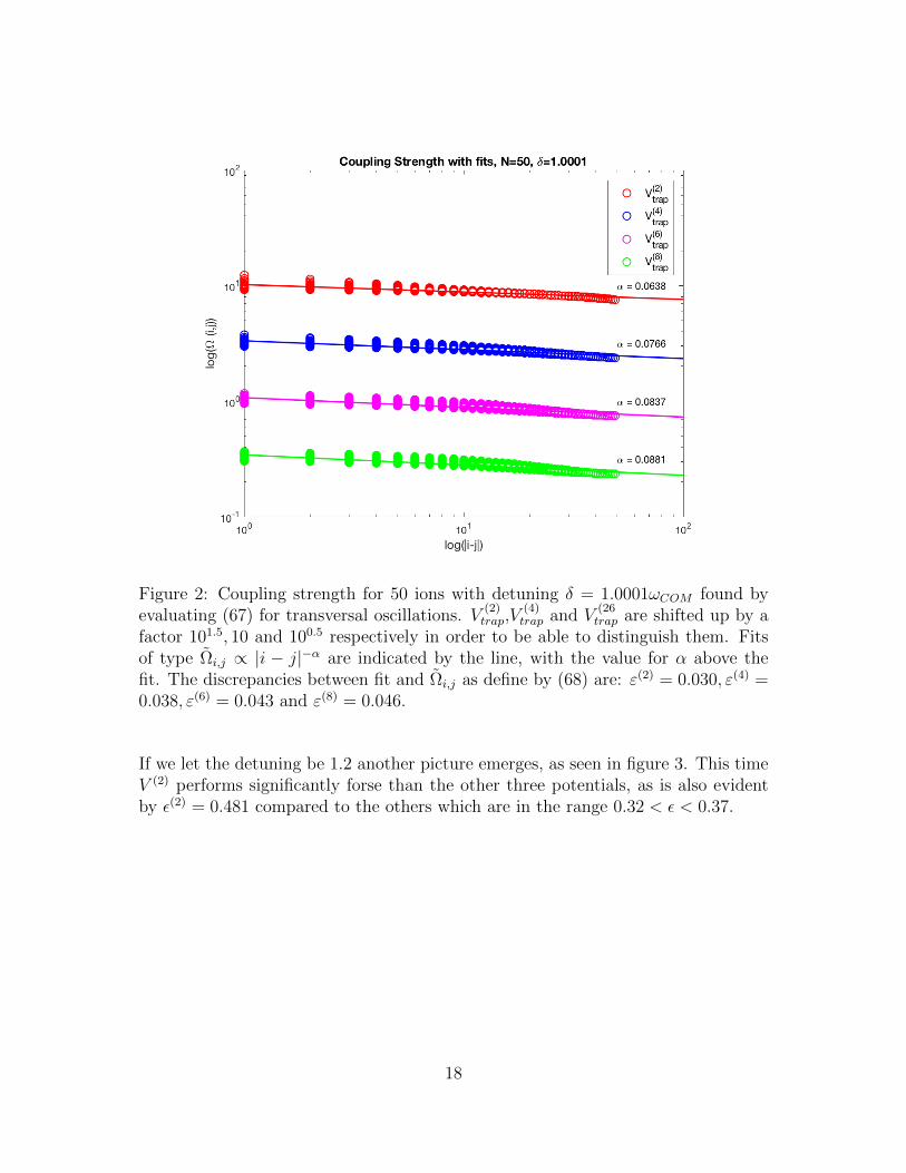
Figure 2: Coupling strength for 50 ions with detuning � = 1.0001!COM found byevaluating (67) for transversal oscillations. V (2)

trap,V(4)trap and V

(26trap are shifted up by a

factor 101.5, 10 and 100.5 respectively in order to be able to distinguish them. Fitsof type ⌦i,j / |i � j|�↵ are indicated by the line, with the value for ↵ above thefit. The discrepancies between fit and ⌦i,j as define by (68) are: "(2) = 0.030, "(4) =0.038, "(6) = 0.043 and "

(8) = 0.046.

If we let the detuning be 1.2 another picture emerges, as seen in figure 3. This timeV

(2) performs significantly forse than the other three potentials, as is also evidentby ✏

(2) = 0.481 compared to the others which are in the range 0.32 < ✏ < 0.37.

18

Figure 3: Coupling strength for 50 ions with detuning � = 1.2!COM found byevaluating (67) for transversal oscillations. V

(2)trap,V

(4)trap and V

(6)trap are shifted up by

a factor 103, 102 and 101 respectively in order to be able to distinguish them. Fitsof type ⌦i,j / |i � j|�↵ are indicated by the line, with the value for ↵ above thefit. The discrepancies between fit and ⌦i,j as define by (68) are: "(2) = 0.481, "(4) =0.361, "(6) = 0.333 and "

(8) = 0.328.

If we let � vary between !COM and 1.2!COM we see that we can indeed get ↵ in therange 0 < ↵ < 3 as seen in figure 4. Likewise we see in figure 5 that for detuningbigger than⇠ 1.02!COM the proposed new trappotential follows the power law closerthan the classical harmonic potential.

5 Possible Improvements

One possible further improvement would be to change the profile of the laser, suchthat it is stronger where the ions are further apart. In the numerical analysis thiswould correspond to change ⌦i, as the e↵ective Hamiltonian relates to the electricalfield through ⌦i. Now we have assumed that the profile is the same across the chain

19

Figure 4: The interaction range (↵) as a function of the detuning for N=50. All fourpotentials have similar performance with 0 < ↵ < 3. If the detuning is chosen to beclose to the center of mass mode !COM there will be long range interaction. Whileof the detuning is chosen to be further from the center of mass mode the interactionrange will become shorter and the hamiltonian will more or less turn into a nearestneighbour model.

as we chose ⌦i = ⌦j = ⌦. This can be done independently of proposed improvementof changing the trap potential.Another possible improvement is to choose another potential than the ones discussedhere. The whole method discussed in this thesis might be turned around such thatinstead of examining the e↵ects of the well known potentials chosen here, one mightconstruct a potential which will result in equal distance between the ions.

6 Conclusion

The proposed changes to the paul trap presentet in this thesis seems to be animprovement. The ability to simulate long-distance spin-spin coupling for detuningclose to the center of mass mode seems to be preserved. If detuning are chosen to befurther from the center of mass mode the changes proposed will lead to significantimprovements, as the coupling strength obeys a power law much more closely.

20

Figure 5: The discrepancy ✏ between the fit and the calculated values for the couplingstrength as defined in (68). It is evident that the proposed trap potentials V (4)

trap, V(6)trap

and V(8)trapobeys the power law much more strictly for higher detunings, while not

performing significantly worse close to resonant.

References

[1] Richard P. Feynman. Simulating physics with computers. International Journalof Theoretical Physics, 21:467–488, 1982.

[2] J. Zhang, G. Pagano, P. W. Hess, A. Kyprianidis, P. Becker, H. Kaplan, A. V.Gorshkov, Z. X. Gong, and C. Monroe. Observation of a many-body dynamicalphase transition with a 53-qubit quantum simulator. Nature, 551:601 EP –, 112017.

[3] Joseph W. Britton, Brian C. Sawyer, Adam C. Keith, C. C. Joseph Wang,James K. Freericks, Hermann Uys, Michael J. Biercuk, and John J. Bollinger.Engineered two-dimensional ising interactions in a trapped-ion quantum simu-lator with hundreds of spins. Nature, 484:489 EP –, 04 2012.

[4] D.F.V. James. Quantum dynamics of cold trapped ions with application toquantum computation. Applied Physics B, 66(2):181–190, Feb 1998.

[5] J. P. Schi↵er. Phase transitions in anisotropically confined ionic crystals.Physical Review Letters, 70(6):818, February 1993.

21

[6] P. Jurcevic, B. P. Lanyon, P. Hauke, C. Hempel, P. Zoller, R. Blatt, and C. F.Roos. Quasiparticle engineering and entanglement propagation in a quantummany-body system. Nature, 511:202 EP –, 07 2014.

[7] D.J. Wineland, C. Monroe, W.M. Itano, D. Leibfried, B.E. King, and D.M.Meekhof. Experimental issues in coherent quantum-state manipulation oftrapped atomic ions. J.Res.Natl.Inst.Stand.Tech., 103(3):259, May-June 1998.

[8] Anders Sørensen and Klaus Mølmer. Quantum computation with ions inthermal motion. Phys. Rev. Lett., 82:1971–1974, Mar 1999.

[9] David J. Gri�ths. Introduction to Quantum Mechanics, page 318. Pearsons,2014.

[10] J. J. Sakurai and Jim J. Napolitano. Modern Quantum Mechanics, page 349.Pearsons, 2014.

[11] Klaus Mølmer and Anders Sørensen. Multiparticle entanglement of hot trappedions. Phys. Rev. Lett., 82:1835–1838, Mar 1999.

22