The Effect of an Employer Health Insurance Mandate on ... · The Effect of an Employer Health...

FEDERAL RESERVE BANK OF SAN FRANCISCO

WORKING PAPER SERIES

Working Paper 2009-08 http://www.frbsf.org/publications/economics/papers/2009/wp09-08bk.pdf

The views in this paper are solely the responsibility of the authors and should not be interpreted as reflecting the views of the Federal Reserve Bank of San Francisco or the Board of Governors of the Federal Reserve System.

The Effect of an Employer Health Insurance Mandate on Health Insurance Coverage and the Demand for Labor:

Evidence from Hawaii

Thomas C. Buchmueller University of Michigan

John DiNardo

University of Michigan

Robert G. Valletta Federal Reserve Bank of San Francisco

April 2011

http://www.frbsf.org/publications/economics/papers/2009/wp09-08bk.pdf�

The Effect of an Employer Health Insurance Mandate on Health Insurance Coverage and the Demand for Labor: Evidence from Hawaii

Thomas C. Buchmueller Stephen M. Ross School of Business

University of Michigan 701 Tappan Street

Ann Arbor, MI 48109 Email: [email protected]

John DiNardo

Gerald R. Ford School of Public Policy and Department of Economics

University of Michigan 735 S. State St.

Ann Arbor, MI 48109 Email: [email protected]

Robert G. Valletta Federal Reserve Bank of San Francisco

101 Market Street San Francisco, CA 94105

email: [email protected]

April 2011 JEL Codes: J32, I18, J23 Keywords: health insurance, employment, hours, wages The authors thank Meryl Motika, Jaclyn Hodges, Monica Deza, Abigail Urtz, Aisling Cleary, and Katherine Kuang for excellent research assistance, Jennifer Diesman of HMSA for providing data, and Gary Hamada, Tom Paul, and Jerry Russo for providing essential background on the PHCA. Thanks also go to Nate Anderson, Julia Lane, Reagan Baughman, and seminar participants at Michigan State University, the University of Hawaii, Cornell University, and the University of Illinois (Chicago and Urbana-Champaign) for helpful comments and suggestions on earlier versions of the manuscript. The views expressed in this paper are those of the authors and should not be attributed to the Federal Reserve Bank of San Francisco or the Federal Reserve System.


ABSTRACT We examine the effects of the most durable employer health insurance mandate in the United States, Hawaii’s Prepaid Health Care Act, using Current Population Survey data covering the years 1979 to 2005. We find that Hawaii’s law increased insurance coverage over time for worker groups with low rates of coverage in the voluntary market. We find no statistically significant support for the hypothesis that the mandate reduced wages and employment probabilities. Instead, its primary detectable effect was an increased reliance on part-time workers who are exempt from the law. We arrive at these conclusions in part by use of a variation of the classical Fisher permutation test that compares the magnitude of the estimated “Hawaii effect” to “placebo effects” estimated for the other US states.

1


I. INTRODUCTION

Long before passage of the federal health care reform act in 2010, which eventually will

impose an individual mandate to obtain health insurance, policy makers had considered the

alternative approach of employer health insurance mandates as a strategy for expanding

coverage. At the Federal level, the failed health care reform plans proposed by the Nixon

administration in the early 1970s and the Clinton administration twenty years later both included

an employer mandate. At the state level, laws imposing employer mandates in Massachusetts

(1988), Oregon (1989), Washington (1993), and California (2003) were overturned by voter

referendums or voided due to conflicts with the federal Employee Retirement Insurance Security

Act (ERISA). Since these laws have not been adopted, direct evidence regarding the effects of

an employer sponsored insurance (ESI) mandate is scarce. One state law that has been enforced

for over two decades and therefore provides a potential source of information on ESI mandates is

Hawaii’s Prepaid Health Care Act (PHCA). Hawaii’s mandate requires that essentially all

private sector employers provide health insurance coverage to employees working at least 20

hours per week on a regular basis.

Despite the significance of Hawaii’s law and its relevance to ongoing policy debates,

quantitative research on its effects is limited (Dick 1994, Thurston 1997, Lee et al. 2005). A key

reason for the paucity of research is timing: the PHCA legislation was passed in 1974, five years

before any national survey provided information on health insurance coverage for individuals,

making it difficult to compare outcomes before and after the passage of the law. While the early

passage of the PHCA creates significant research hurdles, it does not preclude a meaningful

2

analysis of the law’s impact. As we show later, because ESI coverage was relatively stable in

Hawaii while it declined in other states over the past few decades, the coverage gap between

Hawaii and other states widened over time, particularly for worker groups with low rates of ESI

coverage. This divergence in coverage, combined with substantial growth in the relative price of

health care over the same period, implies that the cost of complying with the mandate has grown

over time. As a result, data pre-dating the original PHCA legislation is not necessary for testing

the hypothesis that the mandate has had labor market effects.

In this paper we use Current Population Survey (CPS) data for the years 1979 to 2005 to

compare trends in health insurance coverage and three labor market outcomes—wages, hours,

and employment—between Hawaii and the rest of the United States. Compared with previous

work, our analysis is the first to account for the prediction that the effects of Hawaii’s mandate

should be strongest for workers who are unlikely to receive health benefits in a voluntary

market—primarily low-skill workers—and should be minimal for workers with high rates of ESI

coverage in the absence of a mandate. Ours is also the first study to analyze the complete range

of predicted outcomes in a “difference-in-differences” setting: we use repeated cross-sections

from the CPS to compare changes over time in ESI coverage, alternative sources of coverage,

and labor market outcomes between Hawaii and the rest of the nation, conditional on an

extensive set of control variables.

Given the likely influence of unobserved effects at the state level, we take a conservative

approach to statistical inference by relying on a variant of Fisher’s (1935) permutation test. Our

tests entail comparisons of the usual difference in conditional means between the United States

and Hawaii to parallel “placebo” comparisons between each of the other 50 states (plus DC) and

the remainder of the United States. We find that by this metric Hawaii has an unusually high

3

fraction of individuals with ESI coverage compared with other states, and this gap has grown

over time for groups with low coverage rates, consistent with the expected effects of the

mandate. Using the same framework, we find that the increase in ESI coverage was mirrored by

a similar decline in insurance coverage through public sources (e.g., Medicaid). We also

uncover a rising tendency for Hawaiian employers to rely on part-time positions that are exempt

from the law. Like the coverage results, the effects on part-time work are concentrated on

workers with low probabilities of receiving health benefits in the absence of an employer

mandate. By contrast, we find that Hawaii’s distribution of wages and employment has not

diverged significantly from that in other states.

II. BACKGROUND AND PREVIOUS LITERATURE

II.A. Hawaii’s Health Insurance Mandate

Hawaii’s employer mandate legislation (PHCA) was passed in 1974, the same year that

the U.S. Congress passed ERISA, which established Federal regulation of employer-sponsored

benefit programs. ERISA preempts state laws and has been interpreted by the courts as

prohibiting state laws mandating that employers provide health insurance benefits (Mariner

1992). Shortly after it took effect in January of 1975, the PHCA was successfully challenged on

ERISA grounds; this decision was upheld by the U.S. Court of Appeals in 1980 and by the U.S.

Supreme Court in 1981. In 1983, the U.S. Congress granted a permanent ERISA exemption to

PHCA. Because that legislation specified that substantive changes to PHCA would void the

exemption, the law has been largely unchanged since then (Oliver 2004).

The PHCA requires all private-sector employers in Hawaii to provide health insurance to

employees working 20 or more hours per week. Non-complying employers face financial

4

sanctions and can be shut down after 30 days. In addition to low-hours employees, exemptions

also apply to new hires (employed less than four weeks), seasonal employees, commission-only

workers, and “low-wage” employees.1 Employers must pay at least 50% of the premium cost,

and the employee contribution is limited to an amount that is no greater than 1.5% of their

wages. Qualifying health insurance plans are required to contain certain minimal benefits,

including inpatient hospital coverage, emergency room care, maternity care, and medical and

surgical services.

Available evidence suggests that the legal uncertainty surrounding PHCA’s status limited

the law’s impact between its 1975 enactment and the Federal intervention in 1983. One estimate

is that after the law went into effect, private insurance enrollment increased by no more than

5,000 individuals, slightly less than one percent of the state’s working-age population (Friedman

1993, p. 54).2 Moreover, the state suspended employer compliance audits between the first court

ruling in 1977 and exhaustion of the state’s judicial appeals in 1981 (Agsalud 1982, p. 14). On

the other hand, as we show in Section IV, conditional on observable factors, ESI coverage was

already higher in Hawaii than it was in most other states during this early period. This gap

widened after 1983, which is important for our empirical framework.

II.B. The Economics of Employer Mandated Health Insurance

Summers (1989) showed how the labor market effects of an employer benefit mandate

can be analyzed using a simple supply and demand framework. In his analysis, a mandate causes

the labor demand curve to shift back and the labor supply curve to shift out, causing wages to

fall. The magnitude of the wage change, and the effect on hours and employment, will depend

1 Low-wage workers are defined as those with monthly earnings less than 86.67 times the legislated minimum hourly wage. 2 The U.S. GAO (1994, p. 16) also noted limited enrollment increases after the mandate took effect.

5

on how workers’ valuation of the benefit compares with employers’ cost of provision.

In the absence of any pre-existing market failures, the benefit will be voluntarily provided

to workers whose valuation exceeds employers’ cost. Therefore, such workers should not be

directly affected by a mandate. Instead, the most important effects of a mandate will be on

workers who would not otherwise receive the benefit, either because their valuation falls short of

its cost or because their wage is close to the minimum wage and therefore cannot be reduced

enough to offset the cost of the benefit. Thus, the effects of the mandate on ESI coverage should

be largest for low-wage, low-skill workers, who generally exhibit low rates of coverage in a

voluntary market. Some of this increase in coverage may be offset by declines in coverage

provided to working spouses.3 In addition, increases in ESI coverage among low-wage workers

may offset coverage through public sources such as Medicaid.

For workers most affected by the mandate, whose valuation of ESI falls short of its cost,

the wage reduction arising from the market adjustment to the mandate will fall short of the cost

of the benefit. Employers will therefore face incentives to substitute exempt for covered

workers. If this type of adjustment is not sufficient to offset the remaining costs of the mandate,

relative labor costs rise for covered workers and employers may act to reduce employment of

these workers. We test for such effects in our empirical section, focusing on worker groups

whose ESI coverage rates rose by the largest amount in response to the mandate.

II.C. Past Research on Hawaii’s Mandate

Any analysis of the PHCA must begin by estimating the law’s effect on insurance

coverage. Several prior studies used cross-sectional data to compare insurance coverage in

3The PHCA requires employers to cover a large share of the premiums for employees but imposes weaker requirements regarding contributions for dependent coverage. As a result, the out-of-pocket cost to employees of adding dependents is not necessarily lower in Hawaii than in other states, and married workers may face incentives to receive own ESI coverage rather than coverage as a dependent.

6

Hawaii and the rest of the nation, with mixed results. Based on a cross-section analysis of

Current Population Survey (CPS) data from the mid-1980s, Dick (1994) concluded that the

PHCA did not raise insurance coverage rates in Hawaii relative to other states. However, the

other studies, which used CPS data from later years in a cross-sectional framework, found that

ESI coverage was significantly higher in Hawaii and attributed this result to the PHCA (Thurston

1997, Lee et al. 2005). Differences in data and research design make it difficult to reconcile

these divergent results.4

To the extent that the PHCA prevented employers in Hawaii from dropping coverage in

response to rising premiums, as was observed for the nation as a whole over the past few

decades, we should expect to see adjustments along other margins, such as wages, hours, or

employment. The existing literature provides limited evidence on these labor market effects.

Thurston (1997) investigated the wage effects of Hawaii’s mandate using data from the 1970 and

1990 Censuses aggregated to the industry level (with ESI coverage measured in 1990 only). He

found mixed evidence for wage reductions due to the expansion of ESI, with results that are

highly sensitive to assumptions regarding counterfactual wage trends.

Thurston also tested for an effect on part-time work, again using aggregated industry data

from the 1970 and 1990 Censuses. His comparisons across industries based on ESI coverage in

1990 provided weak evidence in favor of the claim that the percentage of workers with low hours

increased more in Hawaii than in the rest of the United States. In addition to the inability to

identify changes in ESI coverage over time, a further limitation of his analysis is that the

measures of “low hours” work consistently available in his data used weekly hours cut-offs of 15

4 Relying on anecdotal evidence, some analysts have argued that the passage of PHCA had little immediate effect, but once the law was in place it slowed the erosion of employment based coverage as health care costs rose, leading to growing differences between Hawaii and other states over time (Neubauer 1993; U.S. GAO 1994). Our results discussed in subsequent sections are consistent with this.

7

and 30 hours, which are different than the 20 hour cut-off that defines coverage by the PHCA.

Lee et al.’s cross-sectional analysis also provided suggestive evidence that employers in Hawaii

are more likely to employ workers on low-hour schedules.

Much of the discussion and critique of employer mandates has centered on their potential

negative effects on employment. Several papers argued that for workers near the minimum

wage, an employer mandate will have effects similar to an increase in the minimum wage

(Yelowitz 2003; Baicker and Levy 2007; Burkhauser and Simon 2007). However, neither these

studies nor the prior studies on Hawaii’s PHCA tested whether the law had such a

disemployment effect. Compared with the analyses we conduct below, none of the existing

studies of Hawaii’s PHCA tested for the expected differential impacts of the mandate across

worker groups or investigated changes over time arising from the rising costs of compliance.

III. DATA AND DESCRIPTIVE EVIDENCE

III. A. Sample Construction

Our main analyses rely on annual data from the CPS March and Monthly Outgoing

Rotation Group (MORG) files.5 We constructed repeated cross-sections for years starting with

the availability of health insurance questions in the March survey in 1980 and continuing through

the mid-2000s (survey years 1980-2006, which correspond to the reference years of 1979-2005,

the same as in our MORG files). Unless otherwise indicated we focus on workers age 18-64

who are employed in the private sector (excluding the self employed); we exclude government

5 The March CPS provides information on ESI and other sources of health insurance coverage during the prior calendar year. For the analysis of labor market outcomes, we use the MORG files, which provide data on earnings and hours in their main job at the time of the survey. Compared with the March data, the MORG provides larger sample sizes and is not subject to the recall bias that may affect the retrospective data from the March survey.

8

employees because Hawaii’s PHCA law does not apply to them and their inclusion could bias

the cross-state comparisons (with the exception of their use in falsification tests, as described

below). In our analyses of wages and hours, we exclude observations with imputed values of

those variables. Additional details regarding the characteristics of our data files, variable

definitions, and treatment of imputed and top-coded data are provided in Appendix A. Mean

values of population and job variables for Hawaii and the rest of the U.S. are shown in Appendix

B, Table B1 (not for publication; will be made available online).6

III.B. Rising Costs of the PHCA: ESI Premiums and Coverage

In considering the possible labor market effects of the PHCA, it is important to recognize

that the burden of the mandate increased over time as the growth in health insurance premiums

outstripped growth in prices and wages more generally. While employers in the rest of the

nation also experienced rising insurance costs, unlike Hawaiian employers, they can avoid the

rising costs by dropping ESI coverage.7

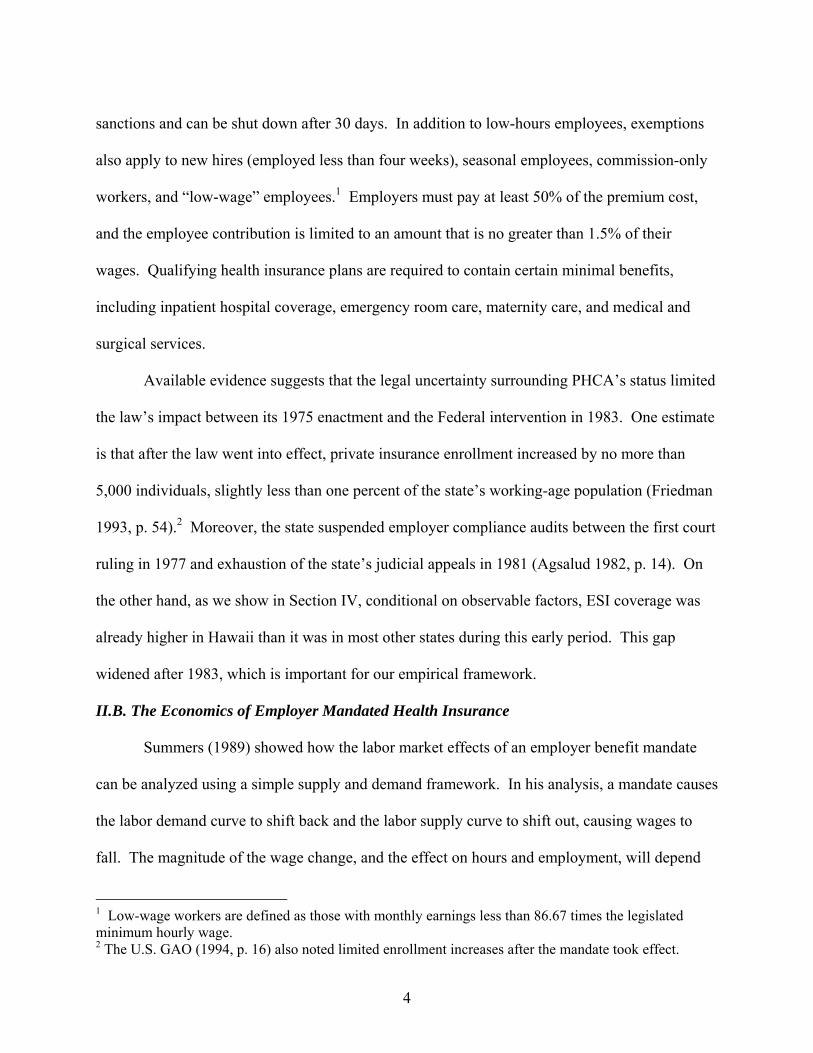
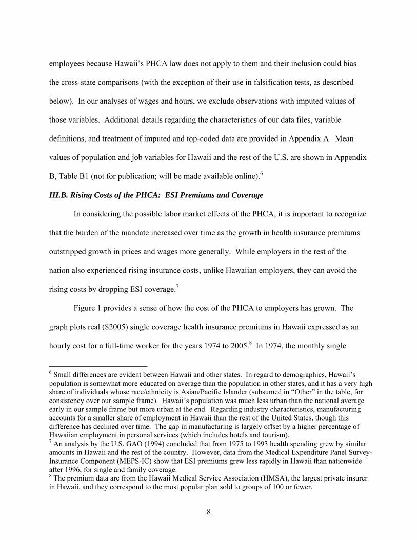
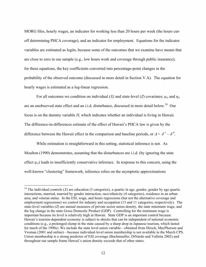
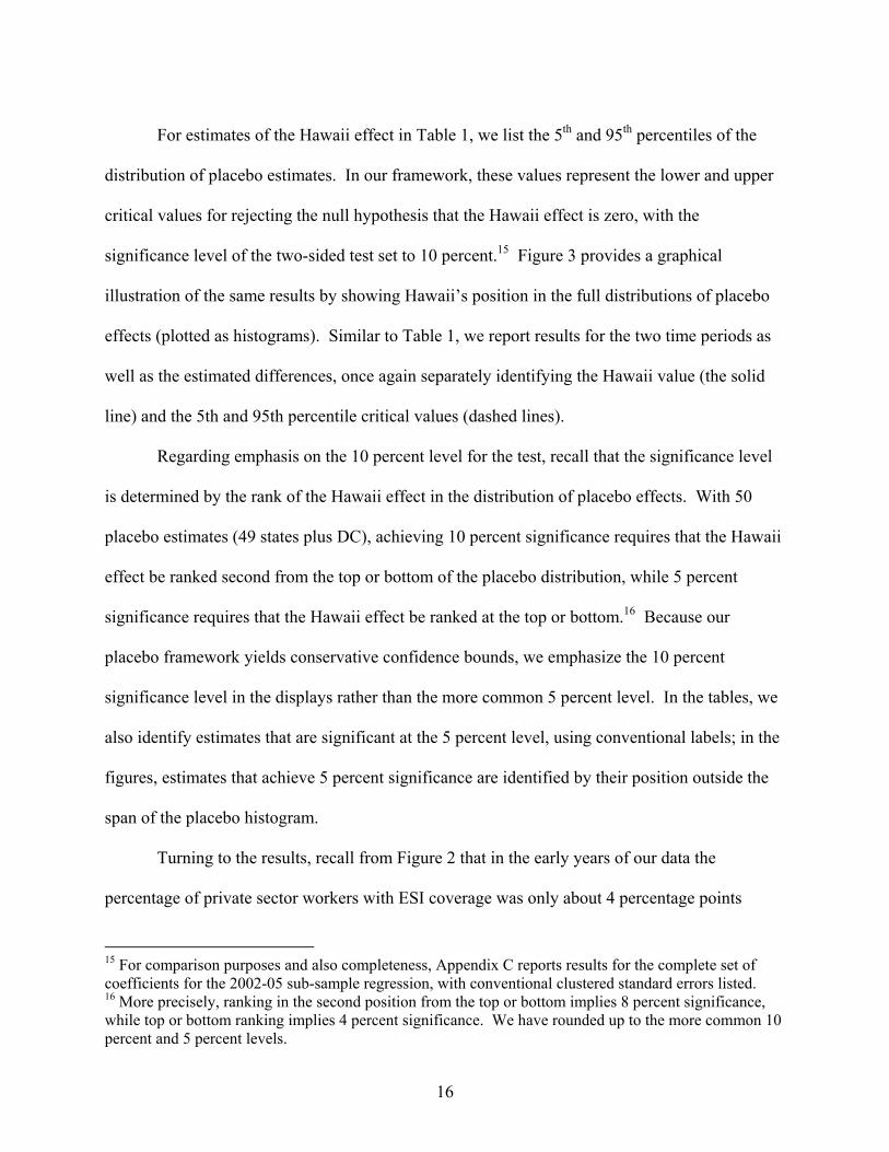
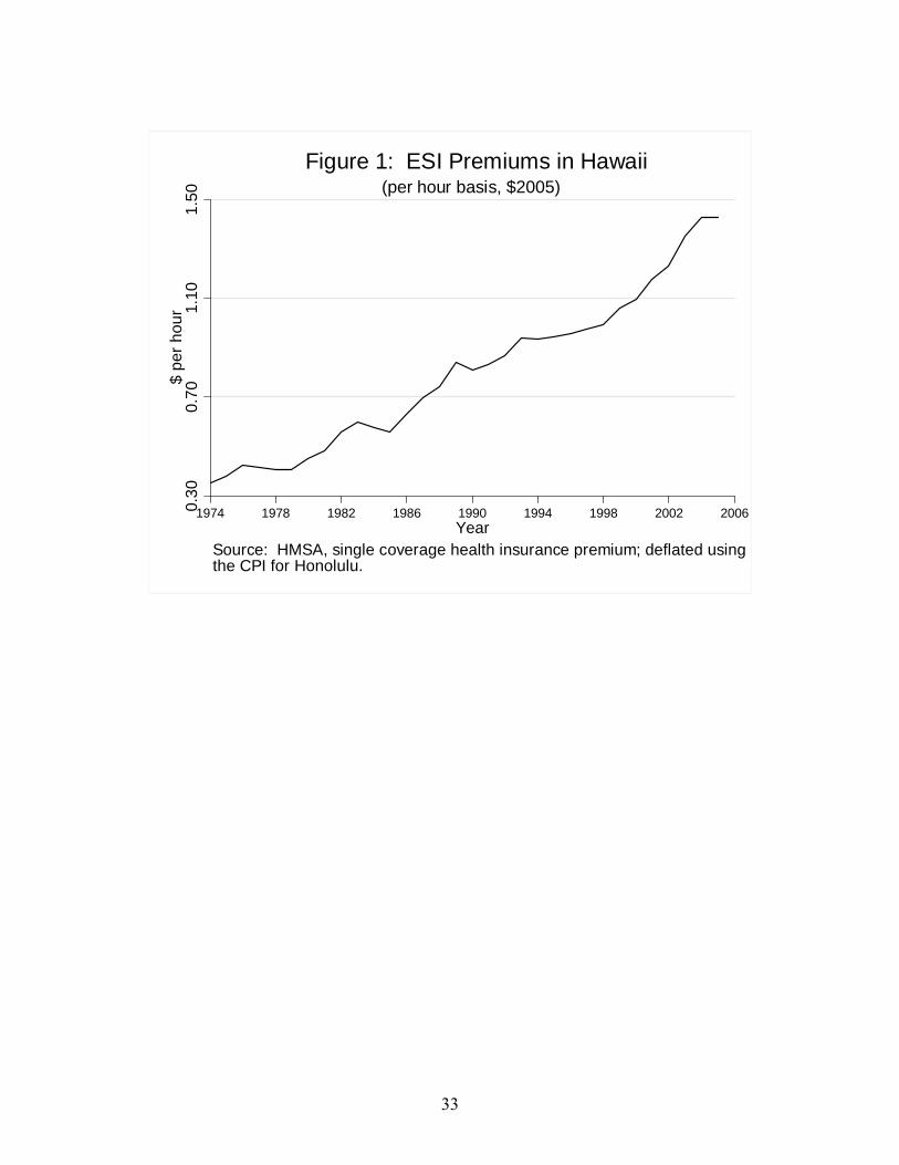
Figure 1 provides a sense of how the cost of the PHCA to employers has grown. The

graph plots real ($2005) single coverage health insurance premiums in Hawaii expressed as an

hourly cost for a full-time worker for the years 1974 to 2005.8 In 1974, the monthly single

6 Small differences are evident between Hawaii and other states. In regard to demographics, Hawaii’s population is somewhat more educated on average than the population in other states, and it has a very high share of individuals whose race/ethnicity is Asian/Pacific Islander (subsumed in “Other” in the table, for consistency over our sample frame). Hawaii’s population was much less urban than the national average early in our sample frame but more urban at the end. Regarding industry characteristics, manufacturing accounts for a smaller share of employment in Hawaii than the rest of the United States, though this difference has declined over time. The gap in manufacturing is largely offset by a higher percentage of Hawaiian employment in personal services (which includes hotels and tourism). 7 An analysis by the U.S. GAO (1994) concluded that from 1975 to 1993 health spending grew by similar amounts in Hawaii and the rest of the country. However, data from the Medical Expenditure Panel Survey-Insurance Component (MEPS-IC) show that ESI premiums grew less rapidly in Hawaii than nationwide after 1996, for single and family coverage. 8 The premium data are from the Hawaii Medical Service Association (HMSA), the largest private insurer in Hawaii, and they correspond to the most popular plan sold to groups of 100 or fewer.

9

coverage premium for a plan meeting the standards of the PHCA was $15.96, which for an

employee working 40 hours per week (assuming 4.3 weeks per month) translated to a cost of 9

cents per hour in current dollars, or 36 cents in 2005 dollars. The cost per hour was only slightly

higher in 1979, the first year in our data set, but then increased steadily thereafter. By 2005 the

monthly premium was $246, or $1.43 per hour for a full-time employee, more than three times

the real cost in 1980. The cumulative increase in the inflation-adjusted costs of insurance

coverage over our sample frame ($1.07 per hour worked) dwarfs the cost of providing health

insurance at the time the law was passed in 1975 ($0.38 per hour) and when it was permanently

authorized by the U.S. Congress in 1983 ($0.60 per hour). This implies that our strategy of

examining cumulative changes over time is likely to dominate the alternative strategy based on

before/after comparisons (which is not possible using available individual data in any event).

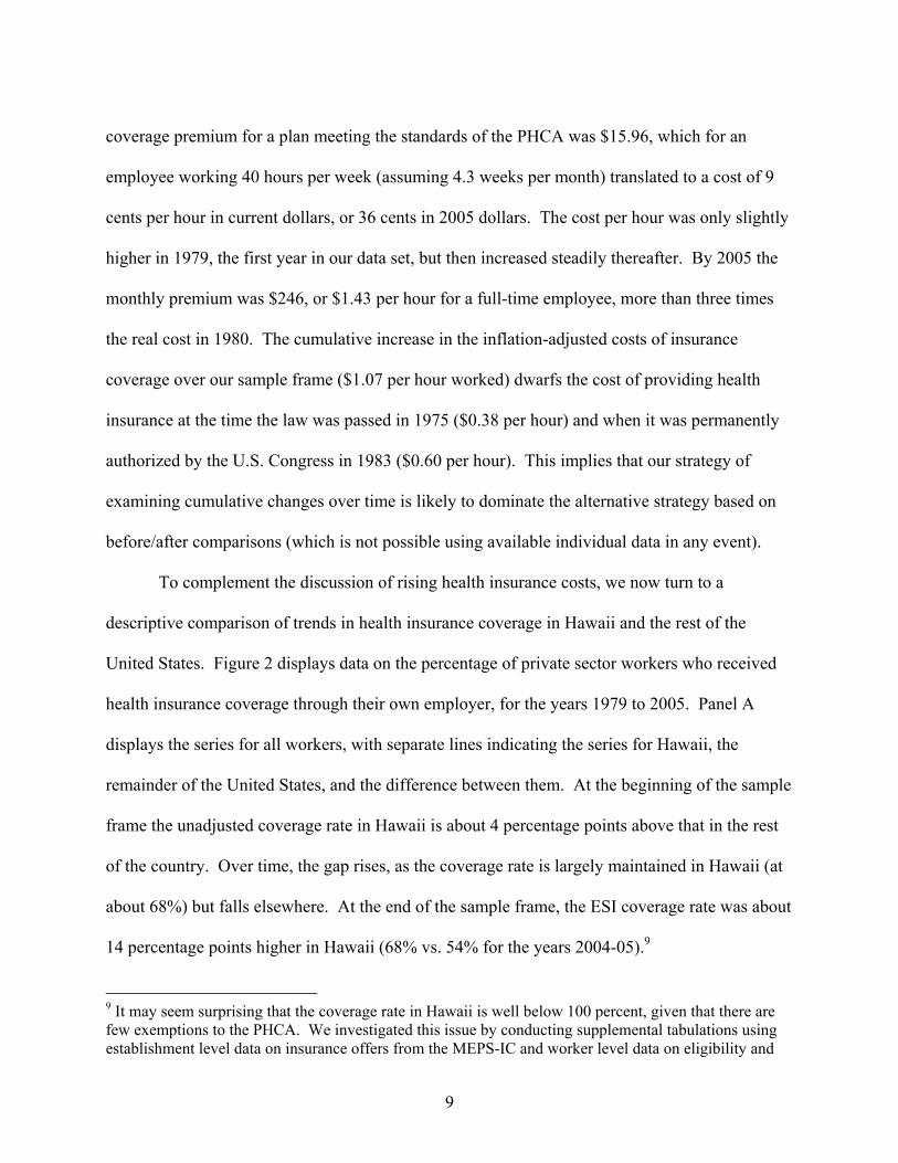
To complement the discussion of rising health insurance costs, we now turn to a

descriptive comparison of trends in health insurance coverage in Hawaii and the rest of the

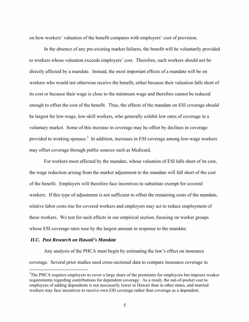
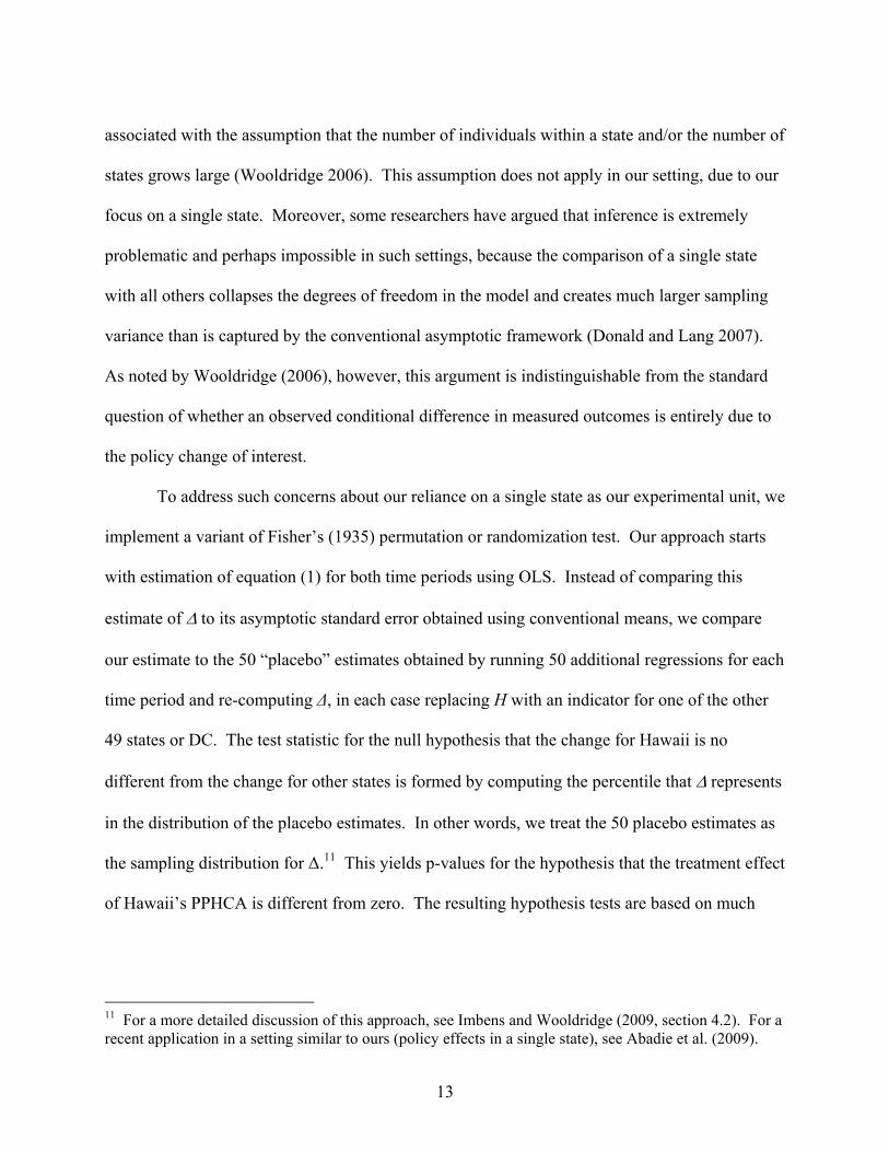
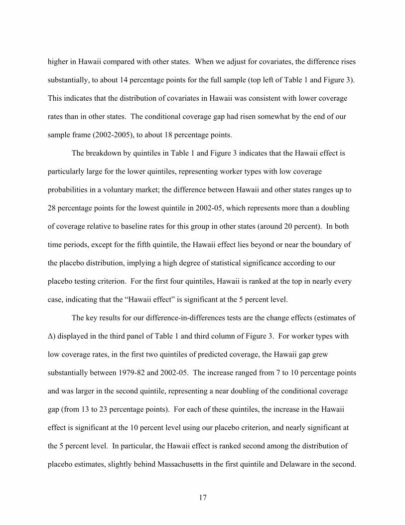
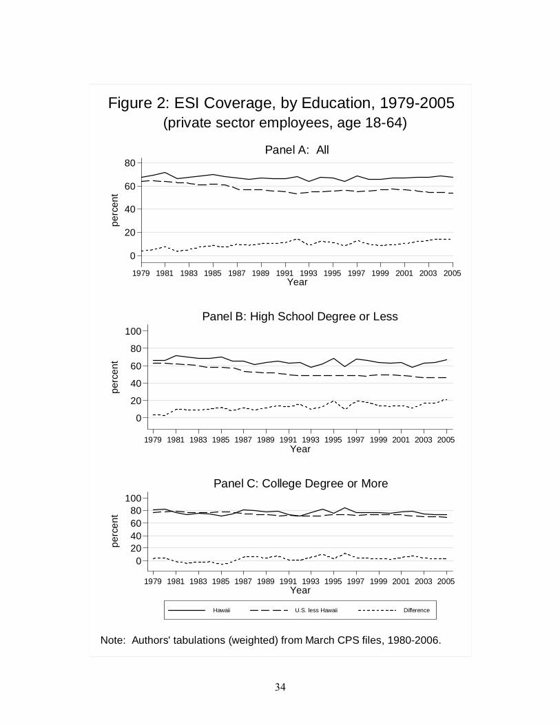
United States. Figure 2 displays data on the percentage of private sector workers who received

health insurance coverage through their own employer, for the years 1979 to 2005. Panel A

displays the series for all workers, with separate lines indicating the series for Hawaii, the

remainder of the United States, and the difference between them. At the beginning of the sample

frame the unadjusted coverage rate in Hawaii is about 4 percentage points above that in the rest

of the country. Over time, the gap rises, as the coverage rate is largely maintained in Hawaii (at

about 68%) but falls elsewhere. At the end of the sample frame, the ESI coverage rate was about

14 percentage points higher in Hawaii (68% vs. 54% for the years 2004-05).9

9 It may seem surprising that the coverage rate in Hawaii is well below 100 percent, given that there are few exemptions to the PHCA. We investigated this issue by conducting supplemental tabulations using establishment level data on insurance offers from the MEPS-IC and worker level data on eligibility and

10

As noted earlier, the basic supply and demand theory predicts that the effect of an

employer mandate on health insurance coverage should be greatest for workers who have low

rates of ESI coverage in the absence of a mandate, such as less skilled workers, and should have

little effect on workers who have a high probability of receiving ESI in a voluntary market. A

simple way to test this prediction is to divide the sample by educational attainment. Panels B

and C of Figure 2 display own ESI coverage rates for workers with a high school degree or less

and a college degree or more (workers with some college but no degree are excluded from these

samples). The results are consistent with our expectations. The rising ESI coverage gap

between Hawaii and the rest of the nation is largely confined to the low education sample. For

that sample, the coverage gap between Hawaii and the rest of the country rose from about 3

percentage points in 1979-1980 to about 19 percentage points in 2004-05. By contrast, for

college educated workers, Hawaii’s ESI coverage gap shifted from positive to negative across

different sub-periods, but it was around 3-4 percentage points at the start and periods of the

sample frame, suggesting little impact of Hawaii’s mandate for this group.

The combination of a large cumulative increase in ESI premium costs and a rising

coverage gap between Hawaii and other states implies that the PHCA mandate has become

increasingly costly to private-sector employers in Hawaii and therefore may have discernible

labor market effects. Testing this proposition more formally requires a statistical conditioning

framework, which we describe in the next section.

take-up from the CPS Contingent Worker Supplements; these data confirmed that most of this gap is accounted for by workers who decline coverage or are not eligible.

11

IV. ECONOMETRIC STRATEGY

IV. A. Permutation Tests

The descriptive results discussed in the preceding section suggest that the ESI coverage

gap between Hawaii and other states rose over our sample frame, particularly for low-skilled

workers. We are interested in testing more formally whether ESI coverage increased over time

in Hawaii relative to other states and also in testing for corresponding changes in labor market

outcomes. We take a difference-in-differences approach that compares changes in ESI coverage

and labor market outcomes in Hawaii to changes in the same outcomes in other states. Our

estimates are derived from cross-sectional regressions run for the baseline period of 1979-1982

(when the legal status of Hawaii’s PPHCA legislation was in dispute) and a later period. Since

we are interested in the long run effects of the law, our analyses focus on the most recent set of

years in our data extract (2002-2005) as the comparison period, though as a robustness test we

experiment with other comparison periods. We estimate separate regressions for the two time

periods rather than a single model with an interaction term, in order to allow for unrestricted

effects of the covariates over time. Also, we pool multiple years in order to ensure adequate

sample sizes for reliable estimation of the Hawaii effect. For each of the periods the model is:

Yist = Xistt + Zstt+Hit δt+ φst + ηit, (t = 0, 1) (1)

These equations are estimated using individual data from the CPS files. In addition to the

time period indicator t in equation (1), i indexes individuals and s indexes states. The dependent

variables Y that we analyze are: from the March CPS files, indicators of health insurance

coverage (own-name ESI as well as alternative sources, as described below); and from the CPS

12

MORG files, hourly wages, an indicator for working less than 20 hours per week (the hours cut-

off determining PHCA coverage), and an indicator for employment. Equations for the indicator

variables are estimated as logits, because some of the outcomes that we examine have means that

are close to zero in our sample (e.g., low hours work and coverage through public insurance);

for these equations, the key coefficients converted into percentage-point changes in the

probability of the observed outcome (discussed in more detail in Section V.A). The equation for

hourly wages is estimated as a log-linear regression.

For all outcomes we condition on individual (X) and state-level (Z) covariates; φst and ηit

are an unobserved state effect and an i.i.d. disturbance, discussed in more detail below.10 Our

focus is on the dummy variable H, which indicates whether an individual is living in Hawaii.

The difference-in-differences estimate of the effect of Hawaii’s PHCA law is given by the

difference between the Hawaii effect in the comparison and baseline periods, or = 1 – 0.

While estimation is straightforward in this setting, statistical inference is not. As

Moulton (1990) demonstrates, assuming that the disturbances are i.i.d. (by ignoring the state

effect φst) leads to insufficiently conservative inference. In response to this concern, using the

well-known “clustering” framework, inference relies on the asymptotic approximations

10 The individual controls (X) are education (5 categories), a quartic in age, gender, gender by age quartic interactions, married, married by gender interaction, race/ethnicity (4 categories), residence in an urban area, and veteran status. In the ESI, wage, and hours regressions (but not the alternative coverage and employment regressions) we control for industry and occupation (13 and 11 categories, respectively). The state-level variables (Z) are annual measures of private sector union density, the state minimum wage, and the log change in the state Gross Domestic Product (GDP). Controlling for the minimum wage is important because its level is relatively high in Hawaii. State GDP is an important control because Hawaii’s tourism-dependent economy is subject to shocks that can be independent of national economic conditions (e.g., a prolonged slump in the state caused by a sharp drop in Japanese tourism, which lasted for much of the 1990s). We include the state level union variable—obtained from Hirsch, MacPherson and Vroman (2001 and online)—because individual-level union membership is not available in the March CPS. Union membership is a strong predictor of ESI coverage (Buchmueller, DiNardo and Valletta 2002) and throughout our sample frame Hawaii’s union density exceeds that of other states.

13

associated with the assumption that the number of individuals within a state and/or the number of

states grows large (Wooldridge 2006). This assumption does not apply in our setting, due to our

focus on a single state. Moreover, some researchers have argued that inference is extremely

problematic and perhaps impossible in such settings, because the comparison of a single state

with all others collapses the degrees of freedom in the model and creates much larger sampling

variance than is captured by the conventional asymptotic framework (Donald and Lang 2007).

As noted by Wooldridge (2006), however, this argument is indistinguishable from the standard

question of whether an observed conditional difference in measured outcomes is entirely due to

the policy change of interest.

To address such concerns about our reliance on a single state as our experimental unit, we

implement a variant of Fisher’s (1935) permutation or randomization test. Our approach starts

with estimation of equation (1) for both time periods using OLS. Instead of comparing this

estimate of to its asymptotic standard error obtained using conventional means, we compare

our estimate to the 50 “placebo” estimates obtained by running 50 additional regressions for each

time period and re-computing Δ, in each case replacing H with an indicator for one of the other

49 states or DC. The test statistic for the null hypothesis that the change for Hawaii is no

different from the change for other states is formed by computing the percentile that represents

in the distribution of the placebo estimates. In other words, we treat the 50 placebo estimates as

the sampling distribution for Δ.11 This yields p-values for the hypothesis that the treatment effect

of Hawaii’s PPHCA is different from zero. The resulting hypothesis tests are based on much

11 For a more detailed discussion of this approach, see Imbens and Wooldridge (2009, section 4.2). For a recent application in a setting similar to ours (policy effects in a single state), see Abadie et al. (2009).

14

more conservative and appropriate confidence intervals than those produced using the standard

clustering alternative.12

IV. B. Accounting for Heterogeneous Policy Effects

As noted earlier, the basic supply and demand theory predicts that the effect of an

employer mandate on health insurance coverage should be greatest for workers who place a low

value on health insurance and therefore have low rates of ESI coverage in the absence of a

mandate, such as younger, less skilled workers, and should have little effect on workers who

have a high probability of receiving ESI in a voluntary market. The results in Figure 2, which

stratifies the data by education, are broadly consistent with this prediction. We can account for

heterogeneous policy effects more precisely by using a full range of explanatory variables to

categorize individuals according to their probability of receiving health benefits in a voluntary

market. To do this we fit the following regression on the complete sample of observations

excluding those in Hawaii, using a logit model estimated separately for each year of data:

Iist = Xistt+ Zstt+ it (2)

In (2), I is an indicator variable for own-name ESI coverage, X and Z are the same controls as in

equation (1), and i, s, and t index individuals, states, and year. Using the results of these

regressions, we fit the probability of ESI coverage for each individual in the full sample

(including Hawaii) and then sort the fitted probabilities and place individuals into quintiles of

this distribution (separately for each year). While education plays an important role in this 12 Our placebo estimates suggest important violations of the assumptions required for the usual clustered standard errors to be appropriate. For example, for some outcomes we investigate below, reliance on clustered standard errors would imply that virtually all of the placebo estimates are statistically significant at conventional levels.

15

prediction equation, other variables are important predictors as well (see Appendix C, intended

for the online version; it lists the results from the ESI equations discussed in the next section).13

V. RESULTS: INSURANCE COVERAGE

V.A. Employer-Sponsored Insurance Coverage

In Table 1 we list the regression-adjusted difference in own name ESI coverage between

Hawaii and other states for the initial period (0) in Panel A, the later period (1) in Panel B, and

the difference between these two estimates () in Panel C. For these numerical estimates and

subsequent results from logit equations, the estimated Hawaii coefficient δ (and placebo

coefficients) are converted into “Population Average Treatment Effects on the Treated” (PATT,

using the terminology of Imbens and Wooldridge 2009), expressed in percentage terms. These

represent the percentage-point change in the probability of the observed outcome arising from

residence in Hawaii (or a placebo state), conditional on other covariates, using the state-specific

distribution of covariates for the calculation.14

13 This approach relates closely to that of Card (1996), who used predictions from a wage equation estimated for non-union workers to examine how the union wage effect varies by skill level. In the statistics literature, such an approach to characterizing “treatment effect heterogeneity” has been called a “prognostic score” (Hansen 2008). 14 For example, the calculation of the PATT (in percentage-point terms) for a specific estimate of the Hawaii effect δ is:

1

1 0

The refer to the fitted logit probabilities (based on equation 1) for a specific individual i, with the coefficient on the Hawaii indicator included (H=1) or excluded (H=0). The PATT is the difference between these fitted probabilities averaged across the complete set of Hawaii observations used in the regression, with observations for other states excluded from the calculation; NH is the number of Hawaii observations. A similar procedure is followed to obtain the PATTs for the placebo estimates. Compared with the alternative calculation based on the entire sample in each case (the “PATE” in Imbens and Wooldridge 2009), the PATT relies on the state-specific covariate values ( 1 ).

16

For estimates of the Hawaii effect in Table 1, we list the 5th and 95th percentiles of the

distribution of placebo estimates. In our framework, these values represent the lower and upper

critical values for rejecting the null hypothesis that the Hawaii effect is zero, with the

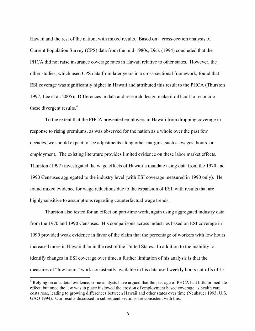
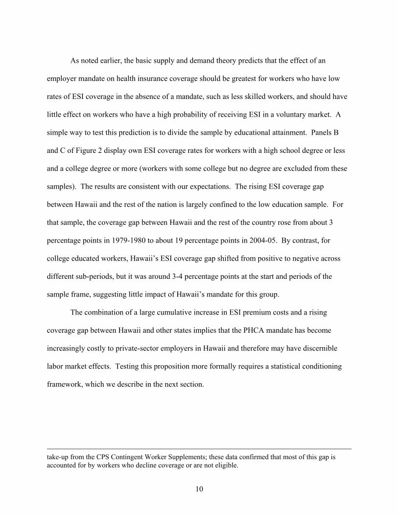
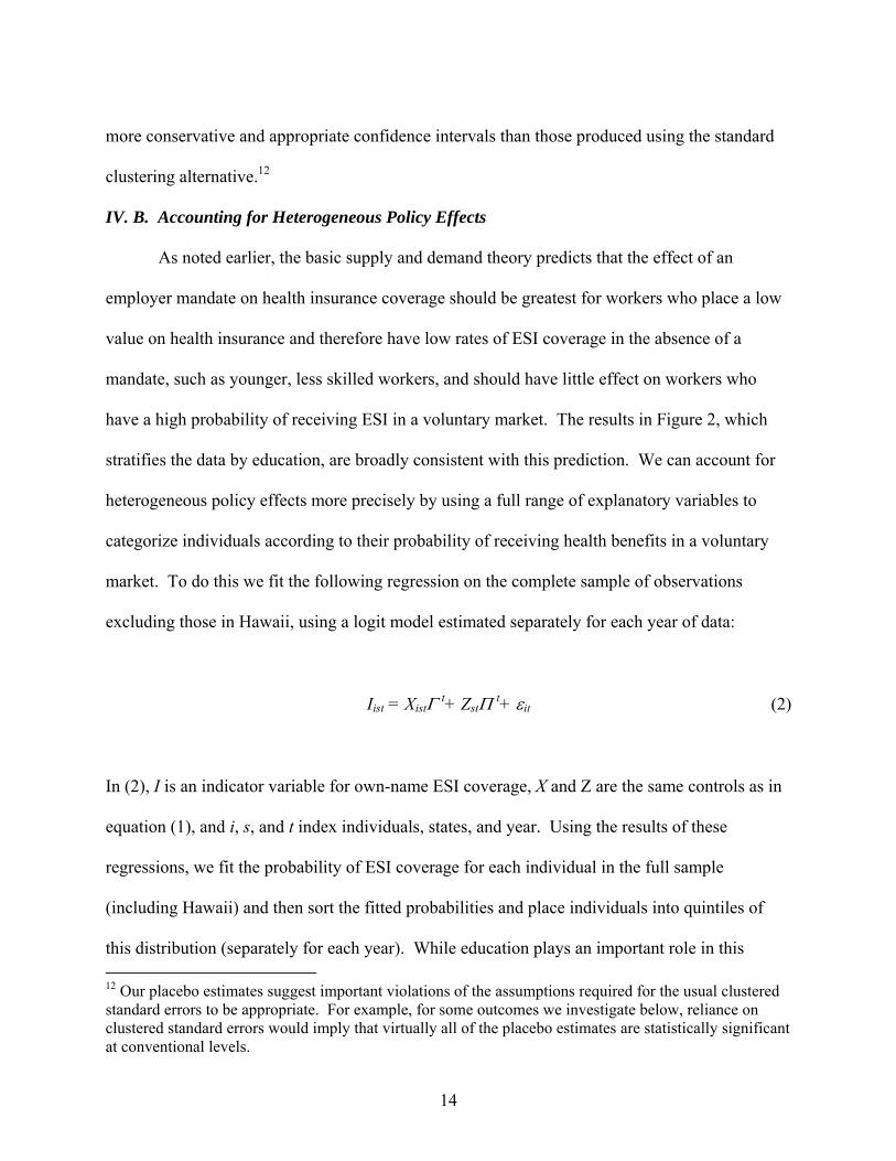
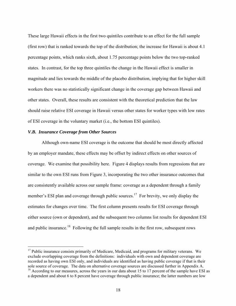
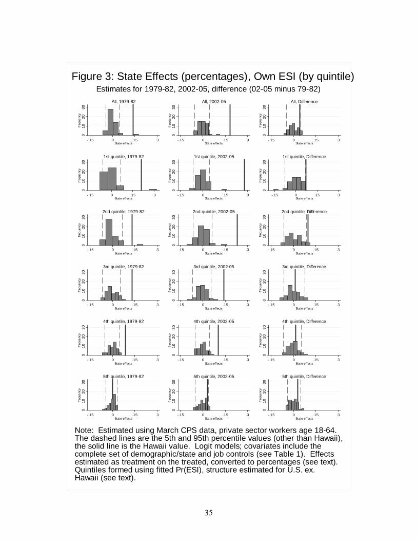
significance level of the two-sided test set to 10 percent.15 Figure 3 provides a graphical

illustration of the same results by showing Hawaii’s position in the full distributions of placebo

effects (plotted as histograms). Similar to Table 1, we report results for the two time periods as

well as the estimated differences, once again separately identifying the Hawaii value (the solid

line) and the 5th and 95th percentile critical values (dashed lines).

Regarding emphasis on the 10 percent level for the test, recall that the significance level

is determined by the rank of the Hawaii effect in the distribution of placebo effects. With 50

placebo estimates (49 states plus DC), achieving 10 percent significance requires that the Hawaii

effect be ranked second from the top or bottom of the placebo distribution, while 5 percent

significance requires that the Hawaii effect be ranked at the top or bottom.16 Because our

placebo framework yields conservative confidence bounds, we emphasize the 10 percent

significance level in the displays rather than the more common 5 percent level. In the tables, we

also identify estimates that are significant at the 5 percent level, using conventional labels; in the

figures, estimates that achieve 5 percent significance are identified by their position outside the

span of the placebo histogram.

Turning to the results, recall from Figure 2 that in the early years of our data the

percentage of private sector workers with ESI coverage was only about 4 percentage points

15 For comparison purposes and also completeness, Appendix C reports results for the complete set of coefficients for the 2002-05 sub-sample regression, with conventional clustered standard errors listed. 16 More precisely, ranking in the second position from the top or bottom implies 8 percent significance, while top or bottom ranking implies 4 percent significance. We have rounded up to the more common 10 percent and 5 percent levels.

17

higher in Hawaii compared with other states. When we adjust for covariates, the difference rises

substantially, to about 14 percentage points for the full sample (top left of Table 1 and Figure 3).

This indicates that the distribution of covariates in Hawaii was consistent with lower coverage

rates than in other states. The conditional coverage gap had risen somewhat by the end of our

sample frame (2002-2005), to about 18 percentage points.

The breakdown by quintiles in Table 1 and Figure 3 indicates that the Hawaii effect is

particularly large for the lower quintiles, representing worker types with low coverage

probabilities in a voluntary market; the difference between Hawaii and other states ranges up to

28 percentage points for the lowest quintile in 2002-05, which represents more than a doubling

of coverage relative to baseline rates for this group in other states (around 20 percent). In both

time periods, except for the fifth quintile, the Hawaii effect lies beyond or near the boundary of

the placebo distribution, implying a high degree of statistical significance according to our

placebo testing criterion. For the first four quintiles, Hawaii is ranked at the top in nearly every

case, indicating that the “Hawaii effect” is significant at the 5 percent level.

The key results for our difference-in-differences tests are the change effects (estimates of

Δ) displayed in the third panel of Table 1 and third column of Figure 3. For worker types with

low coverage rates, in the first two quintiles of predicted coverage, the Hawaii gap grew

substantially between 1979-82 and 2002-05. The increase ranged from 7 to 10 percentage points

and was larger in the second quintile, representing a near doubling of the conditional coverage

gap (from 13 to 23 percentage points). For each of these quintiles, the increase in the Hawaii

effect is significant at the 10 percent level using our placebo criterion, and nearly significant at

the 5 percent level. In particular, the Hawaii effect is ranked second among the distribution of

placebo estimates, slightly behind Massachusetts in the first quintile and Delaware in the second.

18

These large Hawaii effects in the first two quintiles contribute to an effect for the full sample

(first row) that is ranked towards the top of the distribution; the increase for Hawaii is about 4.1

percentage points, which ranks sixth, about 1.75 percentage points below the two top-ranked

states. In contrast, for the top three quintiles the change in the Hawaii effect is smaller in

magnitude and lies towards the middle of the placebo distribution, implying that for higher skill

workers there was no statistically significant change in the coverage gap between Hawaii and

other states. Overall, these results are consistent with the theoretical prediction that the law

should raise relative ESI coverage in Hawaii versus other states for worker types with low rates

of ESI coverage in the voluntary market (i.e., the bottom ESI quintiles).

V.B. Insurance Coverage from Other Sources

Although own-name ESI coverage is the outcome that should be most directly affected

by an employer mandate, these effects may be offset by indirect effects on other sources of

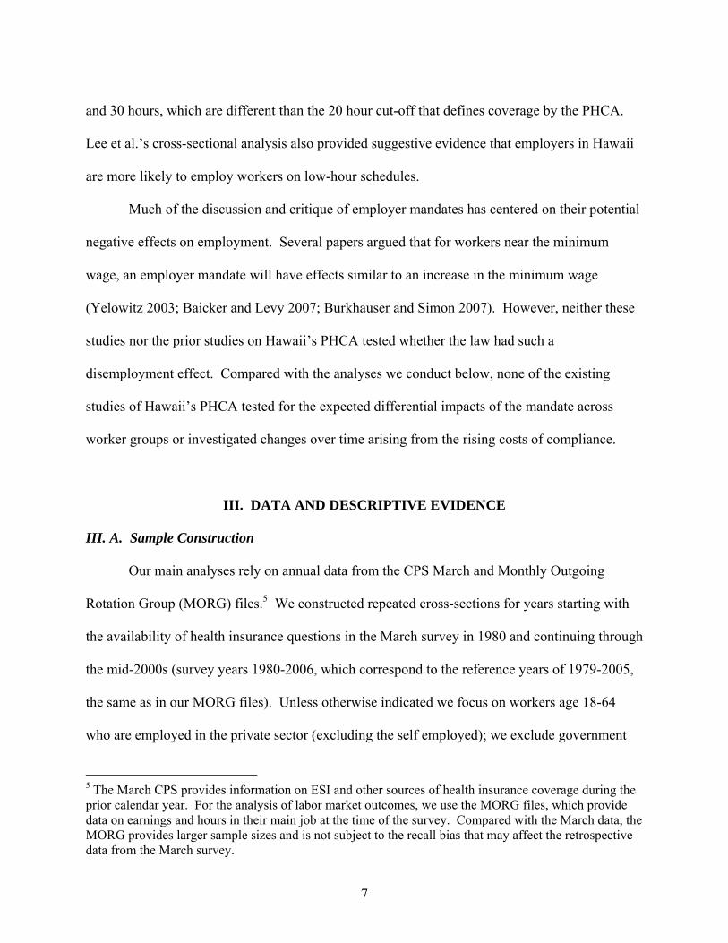
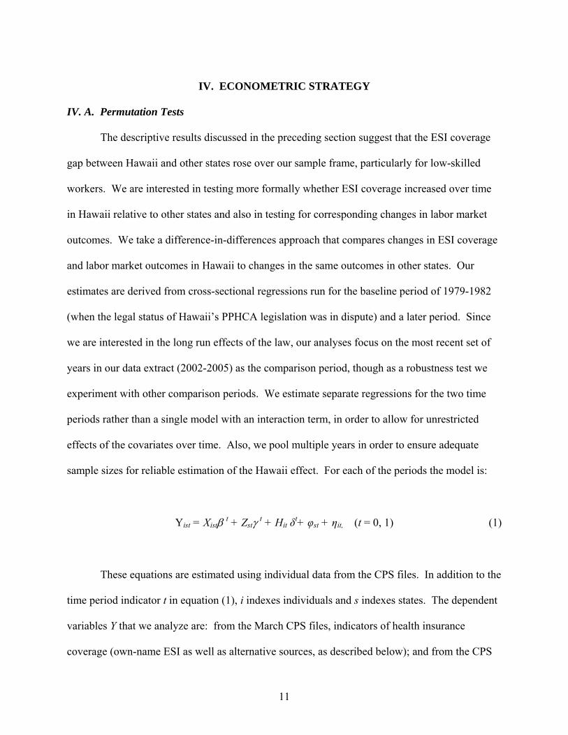
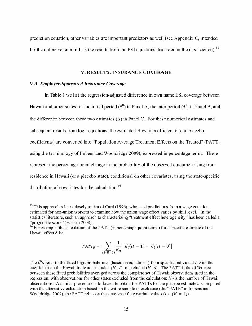
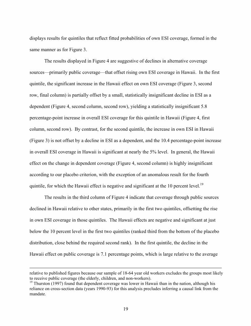
coverage. We examine that possibility here. Figure 4 displays results from regressions that are

similar to the own ESI runs from Figure 3, incorporating the two other insurance outcomes that

are consistently available across our sample frame: coverage as a dependent through a family

member’s ESI plan and coverage through public sources.17 For brevity, we only display the

estimates for changes over time. The first column presents results for ESI coverage through

either source (own or dependent), and the subsequent two columns list results for dependent ESI

and public insurance.18 Following the full sample results in the first row, subsequent rows

17 Public insurance consists primarily of Medicare, Medicaid, and programs for military veterans. We exclude overlapping coverage from the definitions: individuals with own and dependent coverage are recorded as having own ESI only, and individuals are identified as having public coverage if that is their sole source of coverage. The data on alternative coverage sources are discussed further in Appendix A. 18 According to our measures, across the years in our data about 15 to 17 percent of the sample have ESI as a dependent and about 6 to 8 percent have coverage through public insurance; the latter numbers are low

19

displays results for quintiles that reflect fitted probabilities of own ESI coverage, formed in the

same manner as for Figure 3.

The results displayed in Figure 4 are suggestive of declines in alternative coverage

sources—primarily public coverage—that offset rising own ESI coverage in Hawaii. In the first

quintile, the significant increase in the Hawaii effect on own ESI coverage (Figure 3, second

row, final column) is partially offset by a small, statistically insignificant decline in ESI as a

dependent (Figure 4, second column, second row), yielding a statistically insignificant 5.8

percentage-point increase in overall ESI coverage for this quintile in Hawaii (Figure 4, first

column, second row). By contrast, for the second quintile, the increase in own ESI in Hawaii

(Figure 3) is not offset by a decline in ESI as a dependent, and the 10.4 percentage-point increase

in overall ESI coverage in Hawaii is significant at nearly the 5% level. In general, the Hawaii

effect on the change in dependent coverage (Figure 4, second column) is highly insignificant

according to our placebo criterion, with the exception of an anomalous result for the fourth

quintile, for which the Hawaii effect is negative and significant at the 10 percent level.19

The results in the third column of Figure 4 indicate that coverage through public sources

declined in Hawaii relative to other states, primarily in the first two quintiles, offsetting the rise

in own ESI coverage in those quintiles. The Hawaii effects are negative and significant at just

below the 10 percent level in the first two quintiles (ranked third from the bottom of the placebo

distribution, close behind the required second rank). In the first quintile, the decline in the

Hawaii effect on public coverage is 7.1 percentage points, which is large relative to the average

relative to published figures because our sample of 18-64 year old workers excludes the groups most likely to receive public coverage (the elderly, children, and non-workers). 19 Thurston (1997) found that dependent coverage was lower in Hawaii than in the nation, although his reliance on cross-section data (years 1990-93) for this analysis precludes inferring a causal link from the mandate.

20

public coverage rate of about 33 percent in this quintile. It is essentially identical to the

estimated increase in own ESI coverage for this quintile, implying that the increase in own ESI

was exactly offset by a decline in public coverage.

Overall, the alternative coverage results in Figure 4 indicate that the rise in own ESI for

the first two quintiles (from Figure 3 and Table 1) was largely offset by declines in ESI from

public sources, possibly accompanied by some reductions in dependent coverage that may

reduce the cost burden of the mandate. These results help to explain the divergence among prior

studies. Dick’s (1994) conclusion that the PHCA had a minimal impact on insurance coverage

was based on analysis of health insurance from any source, whereas Thurston (1997) and Lee et

al. (2005) focused on own-name ESI.

V.C. Robustness and Falsification Tests

In this section, we discuss the results of several alternative data cuts, which help assess

the robustness of our ESI coverage results and also provide falsification tests. We describe the

results briefly here; the displays are contained in Appendix B, which is not intended for

publication but will appear in an expanded online version of the paper.

Our analysis has focused on the long-run effects of Hawaii’s PPHCA legislation, through

a comparison between the start and end periods of our data (1979-82 and 2002-05). To examine

the sensitivity of our results to the specific periods chosen, Figure B1 provides an analysis of

own ESI coverage parallel to that in Table 3, but with two alternative, intermediate time periods:

1979-82 vs. 1990-93, and 1990-93 vs. 2002-05. For brevity, we only display the results for

changes over time. The results largely confirm the significant Hawaii effect for the first and

second quintiles from Figure 3, although the sub-period breakdown in Figure B1 shows that the

21

increase was most pronounced during the second sub-period for the first quintile and the first

sub-period for the second quintile.

In addition to health insurance benefits, we also examined conditional trends in pension

benefits. Examination of pensions serves as a falsification test for the effects of the PHCA

mandate. If the increase in ESI coverage was accompanied by an increase in pension coverage,

this would suggest that rising ESI was due to unobserved factors affecting employment benefits

in Hawaii in general, rather than a direct effect of the PHCA.

We conducted permutation tests analogous to the ESI tests for two separate pension

variables, indicating whether a workers’ employer offers a pension to any of its employees, and

whether the individual worker is covered by a pension plan (see Appendix A for additional

details regarding these variables). The results are displayed in Appendix B (Figure B2); as

before, and for brevity, we only display the change estimates (Δ).20 These results show that

based on our placebo criterion, there was no increase in relative pension offers or coverage in

Hawaii over our sample frame: the Hawaii effect generally is small and near the middle of the

placebo distribution, or negative in some cases. The absence of an increase in pension

availability and coverage suggests that the increase in ESI coverage in Hawaii (Figure 3) was

likely due to the mandate rather than unobserved effects that increased benefit receipt in general.

Our preceding analyses have focused on private-sector workers, excluding government

employees because Hawaii’s mandate does not apply to them. As such, testing for a Hawaii

effect on the change in ESI coverage for government employees constitutes a additional

20 For this analysis, we formed the quintile groupings based on the fitted probabilities of pension offers and coverage. Separate runs indicated that the results are indistinguishable from those reported here when the quintiles are instead formed using fitted probabilities of ESI coverage instead.

22

falsification test of our finding that the law increased coverage: if the Hawaii effect is caused by

the mandate, we should not find a similar Hawaii effect for government employees.

The results of this test for government employees are displayed in Appendix B (Figure

B3).21 The figure is constructed analogously to Figure 3, with the two sub-periods and change

results displayed in three columns. On average, the point estimates indicate that government

employees in Hawaii have slightly higher coverage rates than do government employees

elsewhere. However, the Hawaii effect in general is statistically insignificant according to our

placebo criterion. Moreover, the only significant increase over time is found for the fifth

quintile, due to a large negative Hawaii effect in the initial sample period. This finding appears

to reflect random elements in the data and does not falsify our private-sector ESI results because

the mandate is not expected to affect the upper quintiles of the predicted ESI coverage

distribution. On balance, these results for government employees do not falsify the findings

regarding rising ESI coverage for private-sector employees.

VI. RESULTS: LABOR MARKET OUTCOMES

Figure 1 showed that Hawaiian employers’ cost of providing health insurance rose

significantly over our sample frame. In addition, the ESI results in Table 1 and Figure 3 showed

that by comparison with other states, own coverage rose significantly in Hawaii for workers

whose characteristics are consistent with low rates of coverage in an unconstrained labor market.

Combined, these sets of results indicate that Hawaii’s mandate created rising costs over time for

employers who hire such workers. Figure 4 showed that some of these costs may have been

21 The quintiles were formed as before but based on the probability of ESI coverage for government employees only; industry and occupation variables were excluded from the list of controls.

23

offset by slight declines in coverage as an ESI dependent, particularly in the first ESI quintile,

implying that the overall mandate costs may be small.

Assuming net positive costs of the mandate, our demand-supply framework from Section

II.B highlights three likely labor market effects. First, to the extent that employers are able to

pass the cost of the mandate on to workers, wage growth for affected workers should be lower in

Hawaii than in other states. If the wage offset is incomplete, perhaps because of a binding

minimum wage, the mandate may affect labor demand by raising the cost of employing less

skilled workers. One potential response is that employers may increase their reliance on part-

time workers who are exempt from the mandate. Alternatively, firms may hire fewer workers

from the available labor force, thereby reducing employment probabilities for worker groups

most likely to be affected by the mandate.

Results for all three labor market outcomes are displayed in Table 2 and Figure 5. For

brevity, we report only the results for the difference-in-differences parameter (Δ); for each

outcome, the full regression results for the most recent sample period are listed in Appendix C

(intended for the online version).

VI.A. Wages

Before turning to our empirical estimates of relative wage changes, it is useful to consider

what constitutes a plausible wage effect of Hawaii’s mandate. We assess this by calculating the

difference effect Δ that we would expect to estimate if the growing costs of the mandate for

employers were fully offset by an equivalent reduction in wages. We set the cost of the mandate

equal to the own-ESI coverage differential between Hawaii and the rest of the United States

multiplied by the full cost of ESI coverage in Hawaii. We focus on the second ESI quintile,

because it exhibits the largest effect on own ESI coverage and combined own and dependent

24

coverage in Figures 3 and 4. The calculations were performed under the assumption that

employers pay 85% of the full direct costs of workers’ health insurance in Hawaii and 80% of

the direct costs in other states.22 The implied decline in relative wages between the baseline

(1979-82) and comparison (2002-05) periods equals 1.6 percent. This represents a very small

change in the observed wage gap over our lengthy sample frame, and as such it is unlikely to be

detectable with acceptable statistical precision using our placebo criterion.

The estimated state effects for wages in difference form are displayed in the first column

of Figure 5 and the top panel of Table 2; the wage regressions were estimated with the log hourly

wage as the dependent variable, and the estimated state effects were translated into percentage

effects on wages using the standard transformation of the coefficient on a dummy variable in a

semi-log equation. The results indicate that wages on average fell slightly (about 3%) in Hawaii

relative to other states over our sample frame (first row, full sample). Across the quintiles,

relative wages in Hawaii fell 2.4% in the first quintile, rose slightly (1.7%) in the second quintile,

and fell by about 4-7.5% in the upper three quintiles.

These wage declines are not readily attributable to Hawaii’s mandate, for two reasons:

(1) the change in wages is wrong-signed in the second quintile (positive rather than negative),

and more generally the estimated wage declines in Hawaii are larger in the higher quintiles; these

findings are inconsistent with the predictions of the supply-demand framework for assessing the

effects of an employer mandate and also with our prior finding of larger ESI effects in the lower

quintiles; (2) the estimated Hawaii effect on wage changes is towards the middle of the

distribution of placebo estimates for other states, so according to our placebo criterion we are

unable to reject the hypothesis that wage changes in Hawaii were the same as in other states. 22 We based these assumptions on tabulations of employee contributions for health insurance plans, using the MEPS-IC data for private-sector establishments in Hawaii and the United States as a whole.

25

As a robustness check, we performed the same placebo test for wage changes using a

sample restricted to workers in the retail industry, who are among the groups most likely to be

affected by the mandate. As shown in Appendix B (Figure B4), the results for this group are

qualitatively similar to the full sample results.

It is important to note that a conventional statistical test would imply large negative wage

effects of Hawaii’s mandate: for the full sample, the t-statistic on the appropriate Hawaii*period

interaction in a fully interacted specification with clustered standard errors is -2.94, indicating a

high degree of statistical significance for the estimated wage declines in Hawaii. However,

applying the same statistical test to the other states effects, we obtain t-statistics that exceed an

absolute value of two in 43 of the 50 cases. As noted in Section IV, this over-rejection of the

null of no significant differences between states highlights why we use the placebo approach.

These results do not necessarily indicate that Hawaii’s ESI mandate had no effect on

wages, but rather that the effect is not detectable in our data using acceptable statistical criteria.

Our inability to reject the null of no wage effect is unsurprising, given the very small magnitude

of the simulated wage offset discussed at the beginning of this sub-section.23 Based solely on

this analysis one might conclude from our permutation testing approach that our design is not

powerful enough to detect effects of Hawaii’s mandate on any labor market outcomes using our

data. However, the results discussed in the next section indicate otherwise.

VI.B. Low Hours Employment

The second column of Figure 4 and second panel of Table 2 display results from

regressions that test whether there has been a long-run trend toward exempt part-time (low-

23 Our point here is similar to that made by Bhattacharya and Vogt (2000) regarding estimated employment effects of state insurance mandates. Using statistical power functions, they argued that the inability to reject the null of no effects in papers such as Gruber (1994) was largely noninformative.

26

hours) work in Hawaii relative to other states, once again showing results for the full sample and

the breakdown by ESI quintiles.24 Individuals are identified as working low hours if they

typically work fewer than 20 hours per week, which is the cutoff for determining whether a

worker is subject to the provisions of the mandate.

In the full sample, the estimate of the change effect for Hawaii is positive and exceeds the

95th percentile critical value from the distribution of placebo estimates; it thereby meets our

standard for statistical significance, indicating that over the entire period the percentage of adults

in short-hour jobs grew significantly faster in Hawaii than in other states. The additional results

in Figure 4 and Table 2 indicate that this full-sample result is driven primarily by the sub-sample

with the lowest probability of receiving ESI. The estimate for this group is statistically

significant at the 10 percent level.25

The estimated shift toward exempt part-time employment is consistent with findings from

past research, including anecdotal evidence cited by the U.S. GAO study (1994, page 15) and

limited quantitative evidence provided in Thurston (1997) and Lee et al. (2005). These findings

suggest employer avoidance behavior in response to the mandate, which reduces the costs of the

mandate and limits its labor market effects. The size of this reduction in mandate costs is

economically meaningful, even though the mandate costs themselves are not large. In particular,

the estimated increase in part-time work in the first ESI quintile for Hawaii is 3.7 percentage

points, compared with an estimated increase in own ESI coverage of 7.1 percentage points

(Table 1, Panel C). Assuming that all of the increase in low-hours employment offset the

24 See Appendix A for details regarding the hours variable. 25 A shift towards low-hours work also is evident in the third quintile. Recall that although the cross-sectional gap in ESI coverage was fairly large for this quintile, it did not grow significantly over time. Therefore, this effect on part-time work reflects the rising burden of the mandate associated with rising health insurance costs for groups that have higher coverage rates in Hawaii than in other states.

27

increase in mandated ESI coverage, had the switch to low-hours employment not occurred, the

increase in ESI coverage would have been 10.8 (7.1+3.7) rather than 7.1 percentage points. The

implied reduction in the costs of the mandate is about one-third (3.7/10.8 = 0.34).26

We subjected these findings for low-hours work to some of the same robustness and

falsification tests that we applied to the own ESI results in Section V.C. The results are

displayed in Appendix B (difference-differences estimate only). First, we estimated the low-

hours models for two alternative, intermediate time periods (1990-93 vs. 1979-82, 2002-05 vs.

1990-93) (Figure B5). The results indicate that the increase in low-hours work was restricted to

the second half of our sample frame. We also estimated the low-hours model for our sample of

government employees (Figure B6). The results suggest a switch to low-hours work in the

higher quintile groups (3rd and 4th; results for the 5th quintile cannot be estimated), which is

inconsistent with the expected effects of the mandate and therefore does not falsify our finding

for private sector workers.

VI.C. Employment

The final outcome we consider is employment, which has been the primary focus of

recent critiques of employer mandates (Yelowitz 2003; Baicker and Levy 2007; Burkhauser and

Simon 2007). The last column of Table 2 and bottom panel of Figure 5 displays results from

26 The estimated increase in low-hours employment is of moderate size compared with its base incidence in the first ESI quintile. The share of low-hours employment in this group ranged from about 10-16 percent across our sample frame (with a downward trend evident over time), and the increase of 3.7 percentage points represents about a 25-35% increase relative to this base level. Readers may note also that the switch to low-hours employment was larger in the first ESI quintile than in the second, despite the larger increase in ESI in the second quintile (from Table 1). This pattern likely arises because employers’ incentives to substitute towards low-hours employment depend not just on the mandate costs but also on detailed characteristics of their production functions that determine the costs of adjusting employees’ work schedules. Such costs are likely to be small for the low-skill workers most affected by the mandate.

28

regressions that use an indicator for employment status as the dependent variable.27 The

specification of these regressions is similar to the model used for wages and part-time work.

However, the sample now consists of all adults 18 to 64 years old (not just those who are

employed) and we exclude industry and occupation from the list of controls used in the ESI

prediction and outcome equations. The results are similar to the wage regressions, indicating that

although conditional employment probabilities declined in Hawaii over time, the changes do not

achieve statistical significance at or near the 10 percent level based on our placebo test.28 The

sole exception is the fourth ESI quintile, for which a 6.6 percentage point decline in employment

probabilities was estimated, significant at the 10% level based on our placebo criterion. Because

this group was not subject to significant mandate effects on coverage, we regard this result as

reflecting random elements in the data rather than the impact of the mandate.

VII. DISCUSSION AND CONCLUSIONS

We found that relative ESI coverage rose in Hawaii over time, and the increase was

larger for workers with characteristics that imply low coverage rates in the absence of a mandate,

consistent with the standard supply/demand theory regarding the effects of employer mandates.

This finding meets the stringent standards for statistical significance imposed by our placebo

testing framework, suggesting that it is a result of the state’s employer mandate rather than

random factors at the state level. Our findings regarding alternative coverage sources suggested

that coverage as a dependent on ESI programs may have declined by a small amount, reducing

the cost burden of the mandate, although this finding does not achieve statistical significance.

27 Individuals are identified as employed if they report working positive hours for pay during the reference week for the monthly CPS files; employment can be private, government, or self-employment. 28 The t-statistic on the Hawaii*(time period) interaction in a fully interacted specification with clustered standard errors is -2.70, indicating significance at the 1% level.

29

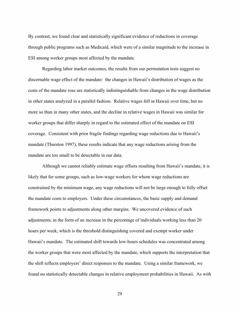
By contrast, we found clear and statistically significant evidence of reductions in coverage

through public programs such as Medicaid, which were of a similar magnitude to the increase in

ESI among worker groups most affected by the mandate.

Regarding labor market outcomes, the results from our permutation tests suggest no

discernable wage effect of the mandate: the changes in Hawaii’s distribution of wages as the

costs of the mandate rose are statistically indistinguishable from changes in the wage distribution

in other states analyzed in a parallel fashion. Relative wages fell in Hawaii over time, but no

more so than in many other states, and the decline in relative wages in Hawaii was similar for

worker groups that differ sharply in regard to the estimated effect of the mandate on ESI

coverage. Consistent with prior fragile findings regarding wage reductions due to Hawaii’s

mandate (Thurston 1997), these results indicate that any wage reductions arising from the

mandate are too small to be detectable in our data.

Although we cannot reliably estimate wage offsets resulting from Hawaii’s mandate, it is

likely that for some groups, such as low-wage workers for whom wage reductions are

constrained by the minimum wage, any wage reductions will not be large enough to fully offset

the mandate costs to employers. Under these circumstances, the basic supply and demand

framework points to adjustments along other margins. We uncovered evidence of such

adjustments, in the form of an increase in the percentage of individuals working less than 20

hours per week, which is the threshold distinguishing covered and exempt worker under

Hawaii’s mandate. The estimated shift towards low-hours schedules was concentrated among

the worker groups that were most affected by the mandate, which supports the interpretation that

the shift reflects employers’ direct responses to the mandate. Using a similar framework, we

found no statistically detectable changes in relative employment probabilities in Hawaii. As with

30

our findings for wages, our data and empirical design do not allow us to rule out employment

reductions arising from the mandate, especially for workers who face low probabilities of

receiving ESI in a voluntary market. However, such effects are small relative to the variation in

other unobserved factors that affect cross-state employment trends.

Our results on net suggest that Hawaii’s health insurance mandate succeeded in raising

ESI coverage rates for worker groups with low coverage rates in an unconstrained environment,

but the costs of this coverage expansion were small compared with other factors affecting labor

demand across states. Our results regarding declines in public coverage indicate that expanded

ESI coverage served largely to shift the coverage burden from public programs to the private

sector. While Hawaii is a somewhat unique state in terms of geography, our analyses indicate

that it is not an outlier in regard to labor market characteristics, suggesting that ESI mandates

may cause limited labor market distortions in other states as well. On the other hand, Hawaii’s

employer mandate has left the state well short of universal coverage, suggesting a need for

alternative approaches to expanding coverage if that is the ultimate policy goal.

31

REFERENCES Abadie, Alberto, Alexis Diamond, and Jens Hanimueller. 2009. “Synthetic Control Methods for

Comparative Case Studies: Estimating the Effect of California’s Tobacco Control Program.” Working Paper, Kennedy School of Government. August.

Agsalud, Joshua C. 1982. Testimony before the U.S. Congress, House Committee on Education

and Labor. ERISA: Exemption from Preemption for Hawaii Prepaid Health Care Act. 97th Congress, 2nd session, January 7 and 8.

Autor, David, Lawrence Katz, and Melissa Kearney. 2008. “Trends in U.S. Wage Inequality:

Revising the Revisionists.” Review of Economics and Statistics 90(2, May): 300-323. Baicker, Katherine and Helen Levy. 2007. “Employer Health Insurance Mandates and the Risk

of Unemployment,” National Bureau of Economic Research Working Paper No. 13528. Bhattacharya, Jay, and William Vogt. 2000. “Could We Tell if Health Insurance Mandates

Cause Unemployment? A Note on the Literature.” Working Paper, Rand Corporation.. Buchmueller, Thomas C., John DiNardo, and Robert G. Valletta. 2002. “Union Effects on

Health Insurance Provision and Coverage in the United States.” Industrial and Labor Relations Review 55(4, July): 610-627.

Burkhauser, Richard and Kosali Simon. 2007. “Who Gets What From Employer Pay or Play

Mandates?” National Bureau of Economic Research Working Paper No. 13578. Card, David. 1996. “The Effect of Unions on the Structure of Wages: A Longitudinal

Analysis.” Econometrica 64(4): 957-979. Dick, Andrew. 1994. “Will Employer Mandates Really Work? Another Look at Hawaii.”

Health Affairs (Spring): 343-349. Donald, Stephen G., and Kevin Lang. 2007. “Inference with Difference-in-Differences and

Other Panel Data.” Review of Economics and Statistics 89(2, May): 221-233. Fisher, R.A. 1935. The Design of Experiments. Edinburgh: Oliver and Boyd. Friedman, Emily. 1993. The Aloha Way: Health Care Structure and Finance in Hawaii.

Honolulu: Hawaii Medical Service Association Foundation,. Hansen, Ben B. 2008. “The prognostic analogue of the propensity score." Biometrika 95(2):

481-8.

32

Hirsch, Barry T., David A. Macpherson, and Wayne G. Vroman. 2001. “Estimates of Union Density by State.” Monthly Labor Review 124(7, July): 51-55 (accompanying data online at www.unionstats.com).

Imbens, Guido W. , and Jeffrey M. Wooldridge. 2009. “Recent Developments in the

Econometrics of Program Evaluation.” Journal of Economic Literature 47(1): 5-86. Lee, Sang-Hyop, Gerard Russo, Lawrence H. Nitz, and Abdul Jabbar. 2005. “The Effect of

Mandatory Employer-Sponsored Insurance (ESI) on Health Insurance Coverage and Labor Force Utilization in Hawaii: Evidence from the Current Population Survey (CPS) 1994-2004.” Working paper, Department of Economics, University of Hawaii.

Lemieux, Thomas. 2006. “Increasing Residual Wage Inequality: Composition Effects, Noisy

Data, or Rising Demand for Skills?” American Economic Review 96 (3, June): 461-498. Mariner, Wendy K. 1992. “Problems with Employer-provided Health Insurance -- the

Employee Retirement Income Security Act and Health Care Reform,” New England Journal of Medicine, 1327:1682-1685.

Moulton, Brent. 1990. “An Illustration of a Pitfall in Estimating the Effects of Aggregate

Variables on Micro Units.” Review of Economics and Statistics 72(2): 334-38. Neubauer, Dean. 1993. “A Pioneer in Health System Reform,” Health Affairs, 31-39. Oliver, Thomas. 2004. “State Employer Health Insurance Mandates: A Brief History.” Mimeo,

California HealthCare Foundation, March. http://www.chcf.org/topics/healthinsurance/ coverageexpansion/index.cfm?itemID=109984.

Summers, Lawrence H. 1989. “Some Simple Economics of Mandated Benefits,” American

Economic Review, 79(2):177-183. Thurston, Norman. 1997. “Labor Market Effects of Hawaii’s Mandatory Employer-Provided

Health Insurance,” Industrial and Labor Relations Review, 51(1): 117-138. U.S. General Accounting Office. 1994. “Health Care in Hawaii: Implications for National

Reform.” Report, GAO/HEHS-94-68, February. Wooldridge, Jeffrey M. 2006. “Cluster-Sample Methods in Applied Econometrics: An

Extended Analysis.” Manuscript, Department of Economics, Michigan State University, June.

Yelowitz, Aaron. 2004. “The Economic Impact of Proposition 72 on California Employers.”

Employment Policies Institute Report, September.

33

0.3

00

.70

1.1

01

.50

$ p

er

ho

ur

1974 1978 1982 1986 1990 1994 1998 2002 2006Year

Source: HMSA, single coverage health insurance premium; deflated usingthe CPI for Honolulu.

(per hour basis, $2005)Figure 1: ESI Premiums in Hawaii

34

0

20

40

60

80

pe

rce

nt

1979 1981 1983 1985 1987 1989 1991 1993 1995 1997 1999 2001 2003 2005Year

Panel A: All

0

20

40

60

80

100

pe

rce

nt

1979 1981 1983 1985 1987 1989 1991 1993 1995 1997 1999 2001 2003 2005Year

Panel B: High School Degree or Less

020406080

100

pe

rce

nt

1979 1981 1983 1985 1987 1989 1991 1993 1995 1997 1999 2001 2003 2005Year

Hawaii U.S. less Hawaii Difference

Panel C: College Degree or More

Note: Authors' tabulations (weighted) from March CPS files, 1980-2006.

(private sector employees, age 18-64)Figure 2: ESI Coverage, by Education, 1979-2005

35

01

02

03

0fr

eque

ncy

-.15 0 .15 .3State effects

All, 1979-82

01

02

03

0fr

eque

ncy


All, 2002-05

01

02

03

0fr

eque

ncy


All, Difference

01

02

03

0fr

eque

ncy


1st quintile, 1979-82

01

02

03

0fr

eque

ncy



01

02

03

0fr

eque

ncy


1st quintile, Difference

01

02

03

0fr

eque

ncy


2nd quintile, 1979-82

01

02

03

0fr

eque

ncy



01

02

03

0fr

eque

ncy


2nd quintile, Difference

01

02

03

0fr

eque

ncy


3rd quintile, 1979-82

01

02

03

0fr

eque

ncy



10

20

30

freq

uenc

y


3rd quintile, Difference

01

02

03

0fr

eque

ncy


4th quintile, 1979-82

01

02

03

0fr

eque

ncy



01

02

03

0fr

eque

ncy


4th quintile, Difference

01

02

03

0fr

eque

ncy



01

02

03

0fr

eque

ncy



01

02

03

0fr

eque

ncy



Note: Estimated using March CPS data, private sector workers age 18-64.The dashed lines are the 5th and 95th percentile values (other than Hawaii),the solid line is the Hawaii value. Logit models; covariates include thecomplete set of demographic/state and job controls (see Table 1). Effectsestimated as treatment on the treated, converted to percentages (see text).Quintiles formed using fitted Pr(ESI), structure estimated for U.S. ex.Hawaii (see text).

Estimates for 1979-82, 2002-05, difference (02-05 minus 79-82)

Figure 3: State Effects (percentages), Own ESI (by quintile)

36

05

10

15

freq

uenc

y

-.1 -.05 0 .05 .1State effects

ESI OWN OR DEPENDENT, All

05

10

15

freq

uenc

y


ESI AS DEPENDENT, All

05

10

15

freq

uenc

y


PUBLIC, All

05

10

15

freq

uenc

y


ESI OWN OR DEPENDENT, quintile 1

05

10

15

20

freq

uenc

y


ESI AS DEPENDENT, quintile 1

05

10

15

freq

uenc

y


PUBLIC, quintile 1

05

10

15

20

freq

uenc

y



05

10

15

freq

uenc

y



05

10

15

freq

uenc

y


PUBLIC, quintile 2

05

10

15

20

freq

uenc

y



05

10

15

20

freq

uenc

y



51

01

5fr

eque

ncy


PUBLIC, quintile 3

05

10

15

freq

uenc

y



05

10

15

freq

uenc

y



05

10

15

20

freq

uenc

y


PUBLIC, quintile 4

05

10

15

freq

uenc

y



05

10

15

20

freq

uenc

y



05

10

15

20

freq

uenc

y


PUBLIC, quintile 5


Difference estimates (2002-05 minus 1979-82)

Figure 4: State Effects (percentages), Alternative Coverage (by quintile)

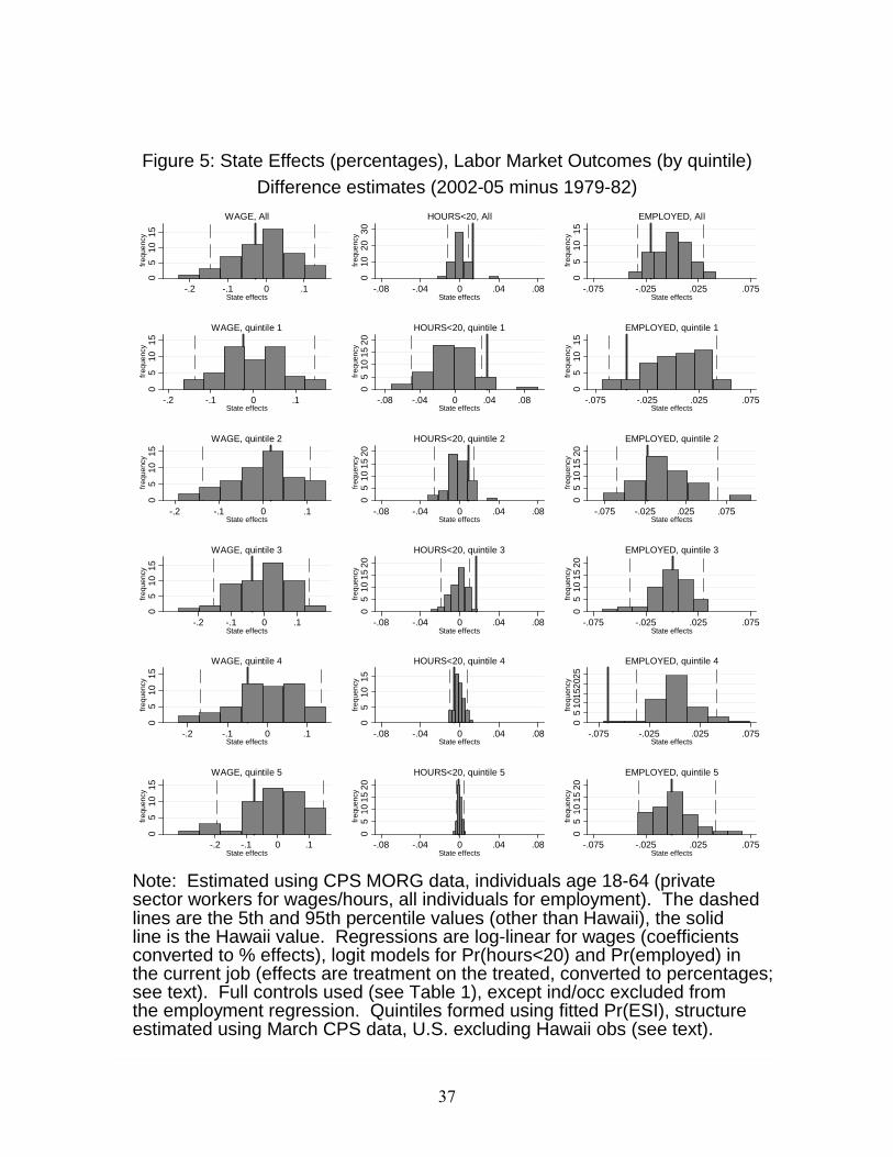
37

05

10

15fr

eque

ncy

-.2 -.1 0 .1State effects

WAGE, All

010

20

30

freq

uenc

y

-.08 -.04 0 .04 .08State effects

HOURS<20, All

05

10

15

freq

uenc

y

-.075 -.025 .025 .075State effects

EMPLOYED, All

05

101

5fr

eque

ncy


WAGE, quintile 1

05

10

152

0fr

eque

ncy

-.08 -.04 0 .04 .08State effects

HOURS<20, quintile 1

05

101

5fr

eque

ncy

-.075 -.025 .025 .075State effects

EMPLOYED, quintile 1

05

10

15fr

eque

ncy


WAGE, quintile 2

05

10

15

20fr

eque

ncy

-.08 -.04 0 .04 .08State effects


05

10

15

20fr

eque

ncy

-.075 -.025 .025 .075State effects


05

10

15fr

eque

ncy


WAGE, quintile 3

05

101

52

0fr

eque

ncy

-.08 -.04 0 .04 .08State effects


05

101

52

0fr

eque

ncy

-.075 -.025 .025 .075State effects


05

101

5fr

eque

ncy


WAGE, quintile 4

05

10

15

freq

uenc

y

-.08 -.04 0 .04 .08State effects


05

101

5202

5fr

eque

ncy

-.075 -.025 .025 .075State effects


05

10

15fr

eque

ncy


WAGE, quintile 5

05

10

15

20fr

eque

ncy

-.08 -.04 0 .04 .08State effects


05

10

15

20fr

eque

ncy

-.075 -.025 .025 .075State effects


Note: Estimated using CPS MORG data, individuals age 18-64 (privatesector workers for wages/hours, all individuals for employment). The dashedlines are the 5th and 95th percentile values (other than Hawaii), the solidline is the Hawaii value. Regressions are log-linear for wages (coefficientsconverted to % effects), logit models for Pr(hours<20) and Pr(employed) inthe current job (effects are treatment on the treated, converted to percentages;see text). Full controls used (see Table 1), except ind/occ excluded fromthe employment regression. Quintiles formed using fitted Pr(ESI), structureestimated using March CPS data, U.S. excluding Hawaii obs (see text).


Figure 5: State Effects (percentages), Labor Market Outcomes (by quintile)

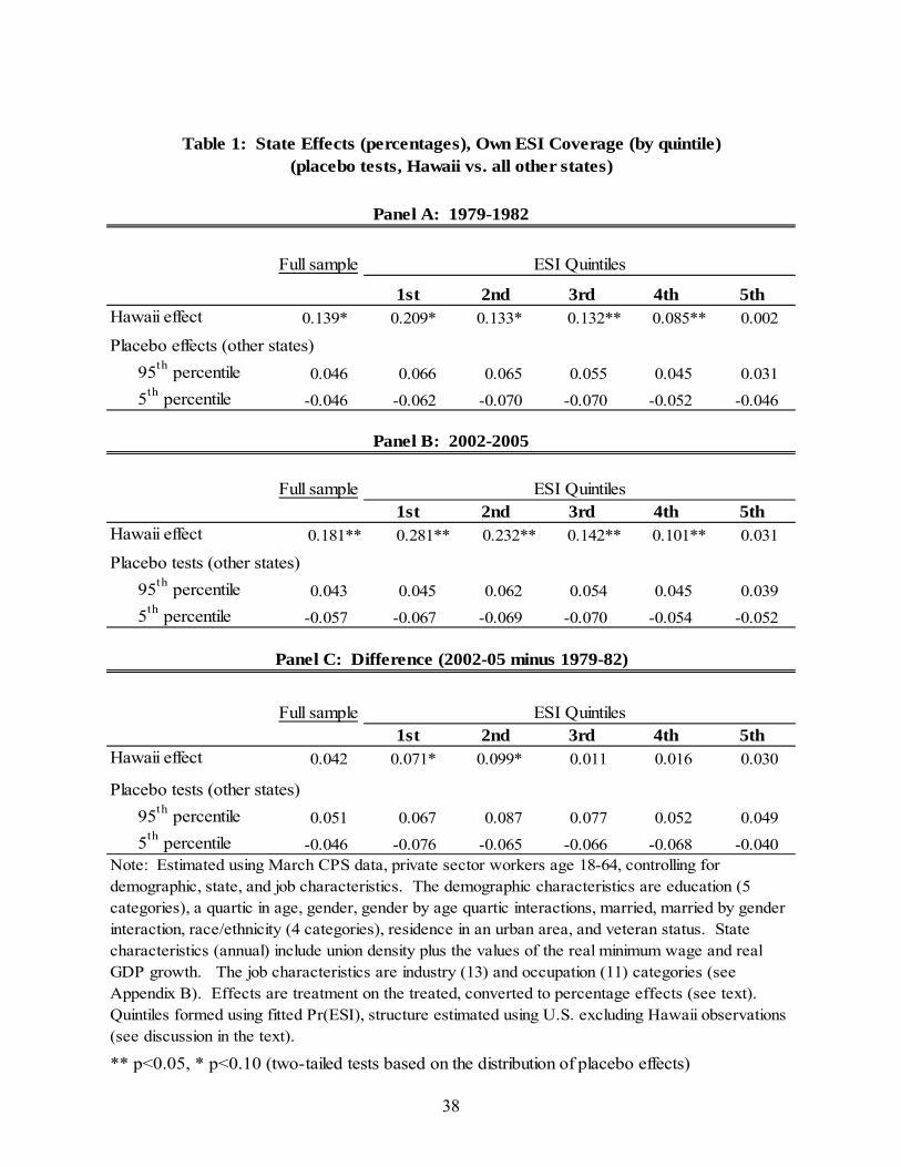
38

Full sample

1st 2nd 3rd 4th 5thHawaii effect 0.139* 0.209* 0.133* 0.132** 0.085** 0.002

95th percentile 0.046 0.066 0.065 0.055 0.045 0.031

5th percentile -0.046 -0.062 -0.070 -0.070 -0.052 -0.046

Full sample1st 2nd 3rd 4th 5th

Hawaii effect 0.181** 0.281** 0.232** 0.142** 0.101** 0.031

95th percentile 0.043 0.045 0.062 0.054 0.045 0.039

5th percentile -0.057 -0.067 -0.069 -0.070 -0.054 -0.052


Hawaii effect 0.042 0.071* 0.099* 0.011 0.016 0.030

95th percentile 0.051 0.067 0.087 0.077 0.052 0.049

5th percentile -0.046 -0.076 -0.065 -0.066 -0.068 -0.040

** p<0.05, * p<0.10 (two-tailed tests based on the distribution of placebo effects)

Note: Estimated using March CPS data, private sector workers age 18-64, controlling for demographic, state, and job characteristics. The demographic characteristics are education (5 categories), a quartic in age, gender, gender by age quartic interactions, married, married by gender interaction, race/ethnicity (4 categories), residence in an urban area, and veteran status. State characteristics (annual) include union density plus the values of the real minimum wage and real GDP growth. The job characteristics are industry (13) and occupation (11) categories (see Appendix B). Effects are treatment on the treated, converted to percentage effects (see text). Quintiles formed using fitted Pr(ESI), structure estimated using U.S. excluding Hawaii observations (see discussion in the text).

Table 1: State Effects (percentages), Own ESI Coverage (by quintile)(placebo tests, Hawaii vs. all other states)

Panel A: 1979-1982

ESI Quintiles

Panel B: 2002-2005

ESI Quintiles

Panel C: Difference (2002-05 minus 1979-82)

ESI Quintiles

Placebo effects (other states)

Placebo tests (other states)


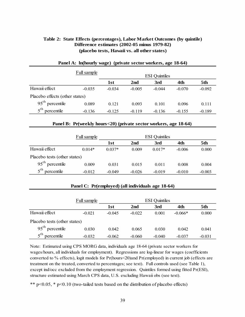
39

Full sample

1st 2nd 3rd 4th 5thHawaii effect -0.035 -0.034 -0.005 -0.044 -0.070 -0.092

95th percentile 0.089 0.121 0.093 0.101 0.096 0.111

5th percentile -0.136 -0.125 -0.119 -0.136 -0.155 -0.189


Hawaii effect 0.014* 0.037* 0.009 0.017* -0.006 0.000

95th percentile 0.009 0.031 0.015 0.011 0.008 0.004

5th percentile -0.012 -0.049 -0.026 -0.019 -0.010 -0.003


Hawaii effect -0.021 -0.045 -0.022 0.001 -0.066* 0.000

95th percentile 0.030 0.042 0.065 0.030 0.042 0.041

5th percentile -0.032 -0.062 -0.060 -0.040 -0.037 -0.031

** p<0.05, * p<0.10 (two-tailed tests based on the distribution of placebo effects)

Note: Estimated using CPS MORG data, individuals age 18-64 (private sector workers for wages/hours, all individuals for employment). Regressions are log-linear for wages (coefficients converted to % effects), logit models for Pr(hours<20)and Pr(employed) in current job (effects are treatment on the treated, converted to percentages; see text). Full controls used (see Table 1), except ind/occ excluded from the employment regression. Quintiles formed using fitted Pr(ESI), structure estimated using March CPS data, U.S. excluding Hawaii obs (see text).

Table 2: State Effects (percentages), Labor Market Outcomes (by quintile)

(placebo tests, Hawaii vs. all other states)

Panel A: ln(hourly wage) (private sector workers, age 18-64)

ESI Quintiles

Placebo effects (other states)

Panel B: Pr(weekly hours<20) (private sector workers, age 18-64)


ESI Quintiles


Panel C: Pr(employed) (all individuals age 18-64)

ESI Quintiles


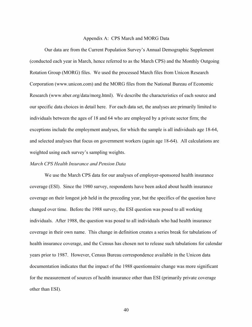
40

Appendix A: CPS March and MORG Data

Our data are from the Current Population Survey’s Annual Demographic Supplement

(conducted each year in March, hence referred to as the March CPS) and the Monthly Outgoing

Rotation Group (MORG) files. We used the processed March files from Unicon Research

Corporation (www.unicon.com) and the MORG files from the National Bureau of Economic

Research (www.nber.org/data/morg.html). We describe the characteristics of each source and

our specific data choices in detail here. For each data set, the analyses are primarily limited to

individuals between the ages of 18 and 64 who are employed by a private sector firm; the

exceptions include the employment analyses, for which the sample is all individuals age 18-64,

and selected analyses that focus on government workers (again age 18-64). All calculations are

weighted using each survey’s sampling weights.

March CPS Health Insurance and Pension Data

We use the March CPS data for our analyses of employer-sponsored health insurance

coverage (ESI). Since the 1980 survey, respondents have been asked about health insurance

coverage on their longest job held in the preceding year, but the specifics of the question have

changed over time. Before the 1988 survey, the ESI question was posed to all working

individuals. After 1988, the question was posed to all individuals who had health insurance

coverage in their own name. This change in definition creates a series break for tabulations of

health insurance coverage, and the Census has chosen not to release such tabulations for calendar

years prior to 1987. However, Census Bureau correspondence available in the Unicon data

documentation indicates that the impact of the 1988 questionnaire change was more significant

for the measurement of sources of health insurance other than ESI (primarily private coverage

other than ESI).

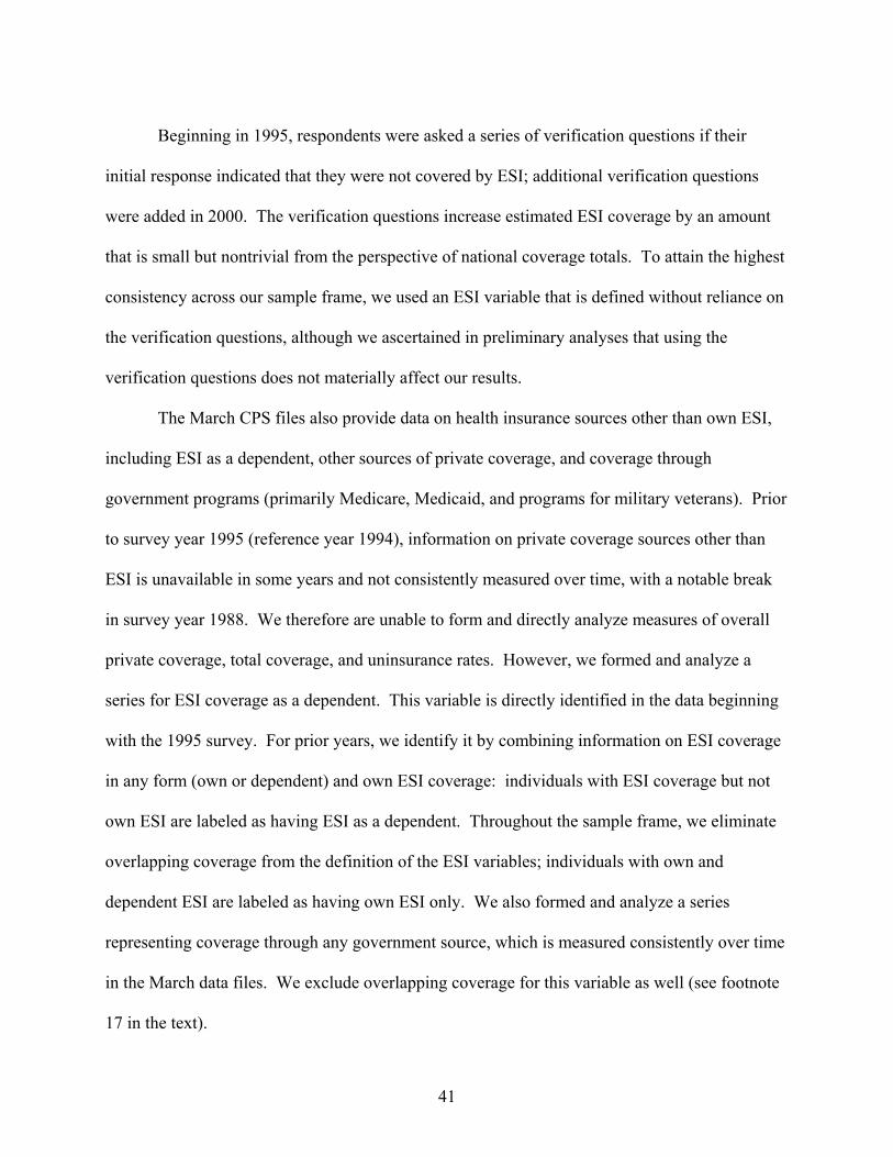
41

Beginning in 1995, respondents were asked a series of verification questions if their

initial response indicated that they were not covered by ESI; additional verification questions

were added in 2000. The verification questions increase estimated ESI coverage by an amount

that is small but nontrivial from the perspective of national coverage totals. To attain the highest

consistency across our sample frame, we used an ESI variable that is defined without reliance on

the verification questions, although we ascertained in preliminary analyses that using the

verification questions does not materially affect our results.

The March CPS files also provide data on health insurance sources other than own ESI,

including ESI as a dependent, other sources of private coverage, and coverage through

government programs (primarily Medicare, Medicaid, and programs for military veterans). Prior

to survey year 1995 (reference year 1994), information on private coverage sources other than

ESI is unavailable in some years and not consistently measured over time, with a notable break

in survey year 1988. We therefore are unable to form and directly analyze measures of overall

private coverage, total coverage, and uninsurance rates. However, we formed and analyze a

series for ESI coverage as a dependent. This variable is directly identified in the data beginning

with the 1995 survey. For prior years, we identify it by combining information on ESI coverage

in any form (own or dependent) and own ESI coverage: individuals with ESI coverage but not

own ESI are labeled as having ESI as a dependent. Throughout the sample frame, we eliminate

overlapping coverage from the definition of the ESI variables; individuals with own and

dependent ESI are labeled as having own ESI only. We also formed and analyze a series

representing coverage through any government source, which is measured consistently over time

in the March data files. We exclude overlapping coverage for this variable as well (see footnote

17 in the text).

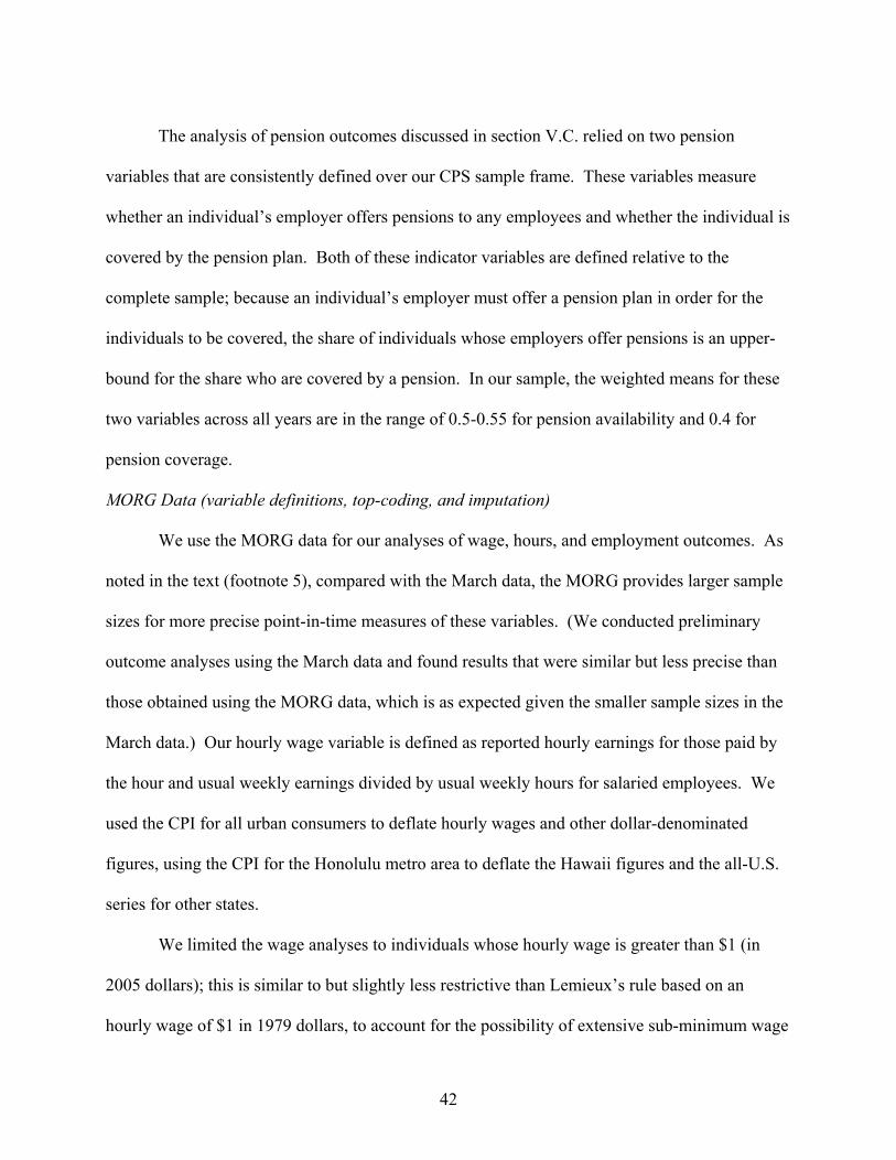
42

The analysis of pension outcomes discussed in section V.C. relied on two pension

variables that are consistently defined over our CPS sample frame. These variables measure

whether an individual’s employer offers pensions to any employees and whether the individual is

covered by the pension plan. Both of these indicator variables are defined relative to the

complete sample; because an individual’s employer must offer a pension plan in order for the

individuals to be covered, the share of individuals whose employers offer pensions is an upper-

bound for the share who are covered by a pension. In our sample, the weighted means for these

two variables across all years are in the range of 0.5-0.55 for pension availability and 0.4 for

pension coverage.

MORG Data (variable definitions, top-coding, and imputation)

We use the MORG data for our analyses of wage, hours, and employment outcomes. As

noted in the text (footnote 5), compared with the March data, the MORG provides larger sample

sizes for more precise point-in-time measures of these variables. (We conducted preliminary

outcome analyses using the March data and found results that were similar but less precise than

those obtained using the MORG data, which is as expected given the smaller sample sizes in the

March data.) Our hourly wage variable is defined as reported hourly earnings for those paid by

the hour and usual weekly earnings divided by usual weekly hours for salaried employees. We

used the CPI for all urban consumers to deflate hourly wages and other dollar-denominated

figures, using the CPI for the Honolulu metro area to deflate the Hawaii figures and the all-U.S.

series for other states.

We limited the wage analyses to individuals whose hourly wage is greater than $1 (in

2005 dollars); this is similar to but slightly less restrictive than Lemieux’s rule based on an

hourly wage of $1 in 1979 dollars, to account for the possibility of extensive sub-minimum wage

43

(tipped) work in Hawaii. We multiplied the value of top-coded earnings observations by 1.4;

this largely follows Lemieux (2006), with the exception that for the sake of consistency over

time, we did not rely on the higher topcode enabled by the use of unedited earnings values for

the years 1989-1993.

We also relied on the usual weekly hours variable to identify individuals who work fewer

than 20 hours per week. Autor, Katz, and Kearney (2008) noted that this hours variable is not

consistently available over time, causing missing observations for the 7-9 percent of the sample

after 1994 who report that their hours of work vary. We excluded these observations from the

sample rather than follow Autor et al’s approach of relying on a variable that measures hours

worked at all jobs during the reference week, because we need precise information on weekly

hours at sample members’ primary job in order to analyze the incidence of low-hours

employment. As noted in the text, we obtain similar results for the hours analysis when we use

the alternative variable based on hours worked in all jobs (the same is true for the wage analysis).

As discussed by Lemieux (2006) and Autor, Katz, and Kearney (2008), the incidence of

imputed values of earnings and hours is substantial in both CPS data sources and has grown over

time. Because the Census “hot deck” matching procedure used for imputation does not restrict

donor matches to individuals in the same state, our results, which focus on one small state, could

be substantially biased if we included imputed observations. We therefore dropped observations

with imputed values of earnings from the analysis of earnings and observations with imputed

values of hours worked from the analysis of low-hours work.29 We followed the procedures

outlined in Lemieux (2006) for identifying imputed earnings observations (including the

29 Because the frequency of imputation is much higher for earnings that it is for hours, our analysis samples are larger for the low-hours equations (see the observation counts for the cross-section equations reported in Appendix C).

44

comparison of unedited and edited earnings values during the years 1989-1993, when the

earnings imputation flags are incorrect). Supplementary analyses conducted for various

specifications indicated that the results are similar when imputed values are included.

Industry and Occupation Codes

Most of our analyses include industry and occupation controls (see Appendix B, Table

B1, for the categories). These definitions have changed over time, with especially large changes

in the 2003 data year, due to the switch to the new NAICS codes. We formed consistent broad

categories over time based on a comprehensive examination of the codes and consequent

reclassification of some industry categories. These recoding schemes are available on request.

45

Appendices B and C: SUPPLEMENTAL RESULTS

NOT FOR PUBLICATION

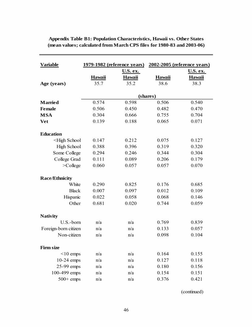
46

Variable

HawaiiU.S. ex. Hawaii Hawaii

U.S. ex. Hawaii

Age (years) 35.7 35.2 38.6 38.3

Married 0.574 0.598 0.506 0.540Female 0.506 0.450 0.482 0.470MSA 0.304 0.666 0.755 0.704Vet 0.139 0.188 0.065 0.071

Education<High School 0.147 0.212 0.075 0.127

High School 0.388 0.396 0.319 0.320Some College 0.294 0.246 0.344 0.304College Grad 0.111 0.089 0.206 0.179

>College 0.060 0.057 0.057 0.070

Race/EthnicityWhite 0.290 0.825 0.176 0.685Black 0.007 0.097 0.012 0.109

Hispanic 0.022 0.058 0.068 0.146Other 0.681 0.020 0.744 0.059

NativityU.S.-born n/a n/a 0.769 0.839

Foreign-born citizen n/a n/a 0.133 0.057Non-citizen n/a n/a 0.098 0.104

Firm size<10 emps n/a n/a 0.164 0.155

10-24 emps n/a n/a 0.127 0.11825-99 emps n/a n/a 0.180 0.156

100-499 emps n/a n/a 0.154 0.151500+ emps n/a n/a 0.376 0.421

(continued)

Appendix Table B1: Population Characteristics, Hawaii vs. Other States

1979-1982 (reference years) 2002-2005 (reference years)

(mean values; calculated from March CPS files for 1980-83 and 2003-06)

(shares)

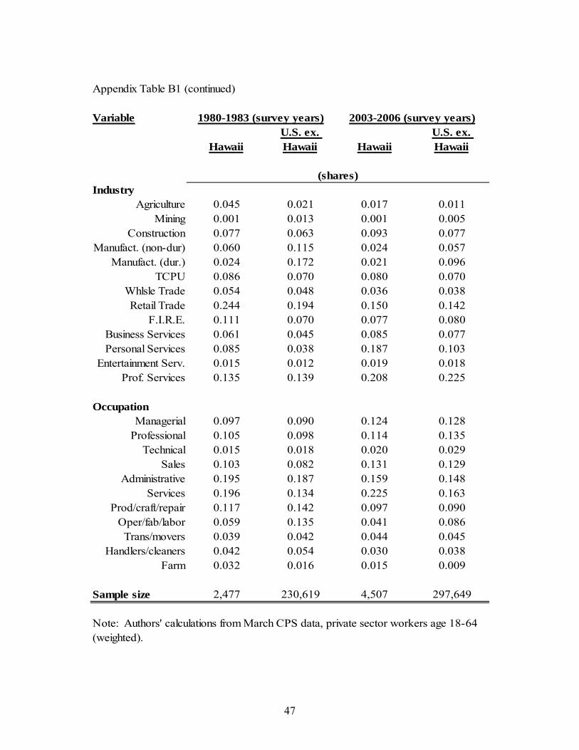
47

Appendix Table B1 (continued)

Variable

HawaiiU.S. ex. Hawaii Hawaii

U.S. ex. Hawaii

IndustryAgriculture 0.045 0.021 0.017 0.011

Mining 0.001 0.013 0.001 0.005Construction 0.077 0.063 0.093 0.077

Manufact. (non-dur) 0.060 0.115 0.024 0.057Manufact. (dur.) 0.024 0.172 0.021 0.096

TCPU 0.086 0.070 0.080 0.070Whlsle Trade 0.054 0.048 0.036 0.038Retail Trade 0.244 0.194 0.150 0.142

F.I.R.E. 0.111 0.070 0.077 0.080Business Services 0.061 0.045 0.085 0.077Personal Services 0.085 0.038 0.187 0.103

Entertainment Serv. 0.015 0.012 0.019 0.018Prof. Services 0.135 0.139 0.208 0.225

OccupationManagerial 0.097 0.090 0.124 0.128

Professional 0.105 0.098 0.114 0.135Technical 0.015 0.018 0.020 0.029

Sales 0.103 0.082 0.131 0.129Administrative 0.195 0.187 0.159 0.148

Services 0.196 0.134 0.225 0.163Prod/craft/repair 0.117 0.142 0.097 0.090

Oper/fab/labor 0.059 0.135 0.041 0.086Trans/movers 0.039 0.042 0.044 0.045

Handlers/cleaners 0.042 0.054 0.030 0.038Farm 0.032 0.016 0.015 0.009

Sample size 2,477 230,619 4,507 297,649

Note: Authors' calculations from March CPS data, private sector workers age 18-64 (weighted).

1980-1983 (survey years) 2003-2006 (survey years)

(shares)

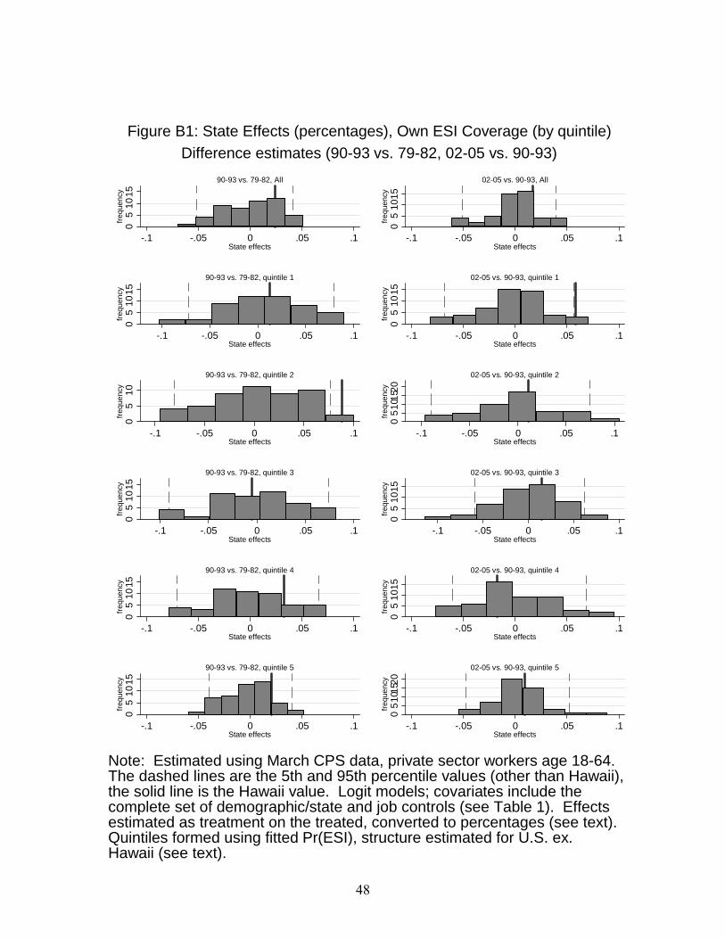
48

05

10

15

freq

uenc

y


90-93 vs. 79-82, All

05

10

15

freq

uenc

y


02-05 vs. 90-93, All

05

10

15

freq

uenc

y


90-93 vs. 79-82, quintile 1

05

10

15

freq

uenc

y


02-05 vs. 90-93, quintile 1

05

10

freq

uenc

y


90-93 vs. 79-82, quintile 2

05

101

520

freq

uenc

y


02-05 vs. 90-93, quintile 2

05

10

15

freq

uenc

y


90-93 vs. 79-82, quintile 3

05

10

15

freq

uenc

y


02-05 vs. 90-93, quintile 3

05

10

15

freq

uenc

y


90-93 vs. 79-82, quintile 4

05

10

15

freq

uenc

y


02-05 vs. 90-93, quintile 4

05

10

15

freq

uenc

y


90-93 vs. 79-82, quintile 5

05

101

520

freq

uenc

y


02-05 vs. 90-93, quintile 5


Difference estimates (90-93 vs. 79-82, 02-05 vs. 90-93)

Figure B1: State Effects (percentages), Own ESI Coverage (by quintile)

49

05

10

freq

uenc

y


Pension available, All

05

10

15

freq

uenc

y


Pension coverage, All

05

10fr

eque

ncy


Pension available, quintile 1

05

10

15fr

eque

ncy


Pension coverage, quintile 1

05

10fr

eque

ncy



05

10fr

eque

ncy



05

10

15fr

eque

ncy



05

10fr

eque

ncy



05

101

5fr

equ

ency



05

101

5fr

equ

ency



05

1015

freq

uen

cy



05

1015

freq

uen

cy



Note: Estimated using March CPS data, private sector workers age 18-64.The dashed lines are the 5th and 95th percentile values (other than Hawaii),the solid line is the Hawaii value. Logit models; covariates include thecomplete set of demographic/state and job controls (see Table 1). Effectsestimated as treatment on the treated, converted to percentages (see text).Quintiles formed using fitted Pr(pension), structure estimated for U.S. ex.Hawaii (see text).


Figure B2: State Effects (percentages), Pensions (by quintile)

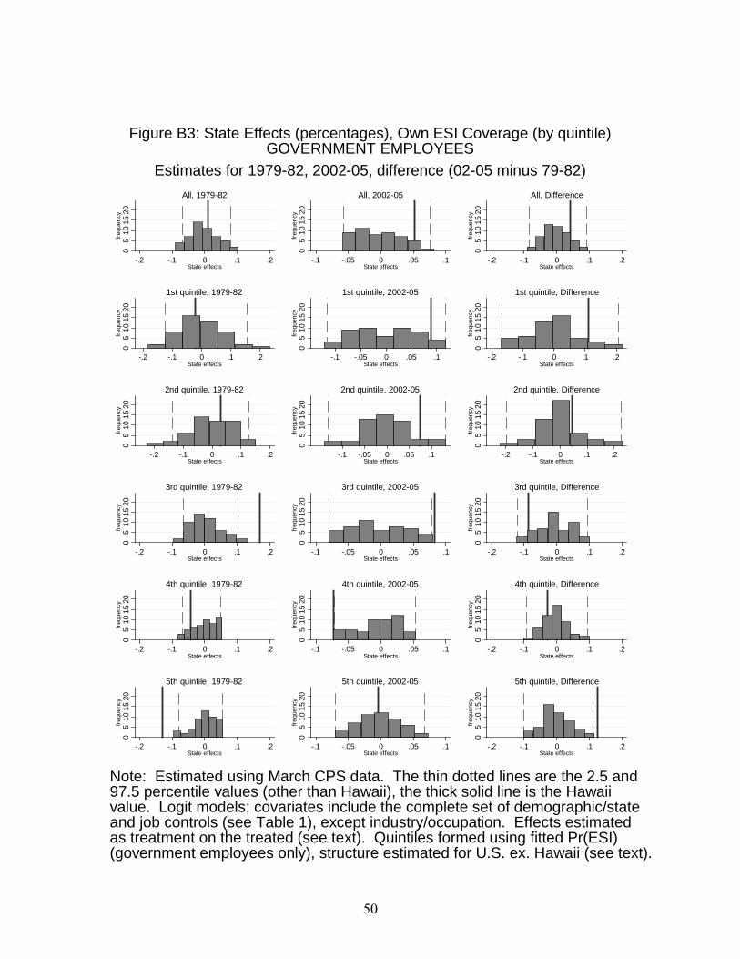
50

05

10

15

20fr

eque

ncy


All, 1979-82

05

10

15

20fr

eque

ncy


All, 2002-05

05

10

15

20fr

eque

ncy


All, Difference

05

10

15

20fr

eque

ncy



51

01

520

freq

uenc

y



05

10

15

20fr

eque

ncy


1st quintile, Difference

05

10

15

20fr

eque

ncy



05

10

15

20fr

eque

ncy



05

10

15

20fr

eque

ncy


2nd quintile, Difference

05

10

15

20fr

eque

ncy



05

10

15

20fr

eque

ncy



51

01

520

freq

uenc

y


3rd quintile, Difference

05

101

520

freq

uenc

y



05

101

520

freq

uenc

y



05

101

520

freq

uenc

y



05

101

520

freq

uenc

y



05

101

520

freq

uenc

y



05

101

520

freq

uenc

y



Note: Estimated using March CPS data. The thin dotted lines are the 2.5 and97.5 percentile values (other than Hawaii), the thick solid line is the Hawaiivalue. Logit models; covariates include the complete set of demographic/stateand job controls (see Table 1), except industry/occupation. Effects estimatedas treatment on the treated (see text). Quintiles formed using fitted Pr(ESI)(government employees only), structure estimated for U.S. ex. Hawaii (see text).

Estimates for 1979-82, 2002-05, difference (02-05 minus 79-82)

Figure B3: State Effects (percentages), Own ESI Coverage (by quintile)GOVERNMENT EMPLOYEES

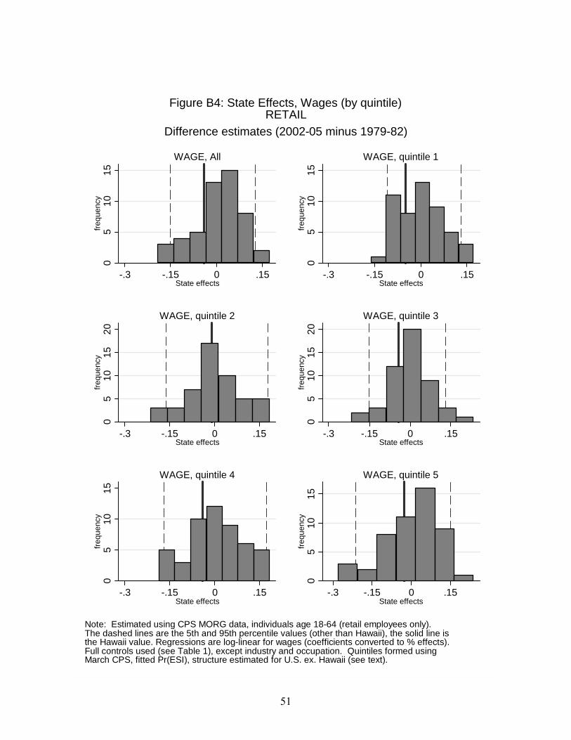
51

05

1015

freq

uenc

y


WAGE, All

05

1015

freq

uenc

y


WAGE, quintile 1

05

1015

20fr

eque

ncy


WAGE, quintile 20

510

1520

freq

uenc

y


WAGE, quintile 3

05

1015

freq

uen

cy


WAGE, quintile 4

05

1015

freq

uen

cy


WAGE, quintile 5

Note: Estimated using CPS MORG data, individuals age 18-64 (retail employees only).The dashed lines are the 5th and 95th percentile values (other than Hawaii), the solid line isthe Hawaii value. Regressions are log-linear for wages (coefficients converted to % effects).Full controls used (see Table 1), except industry and occupation. Quintiles formed usingMarch CPS, fitted Pr(ESI), structure estimated for U.S. ex. Hawaii (see text).


Figure B4: State Effects, Wages (by quintile)RETAIL

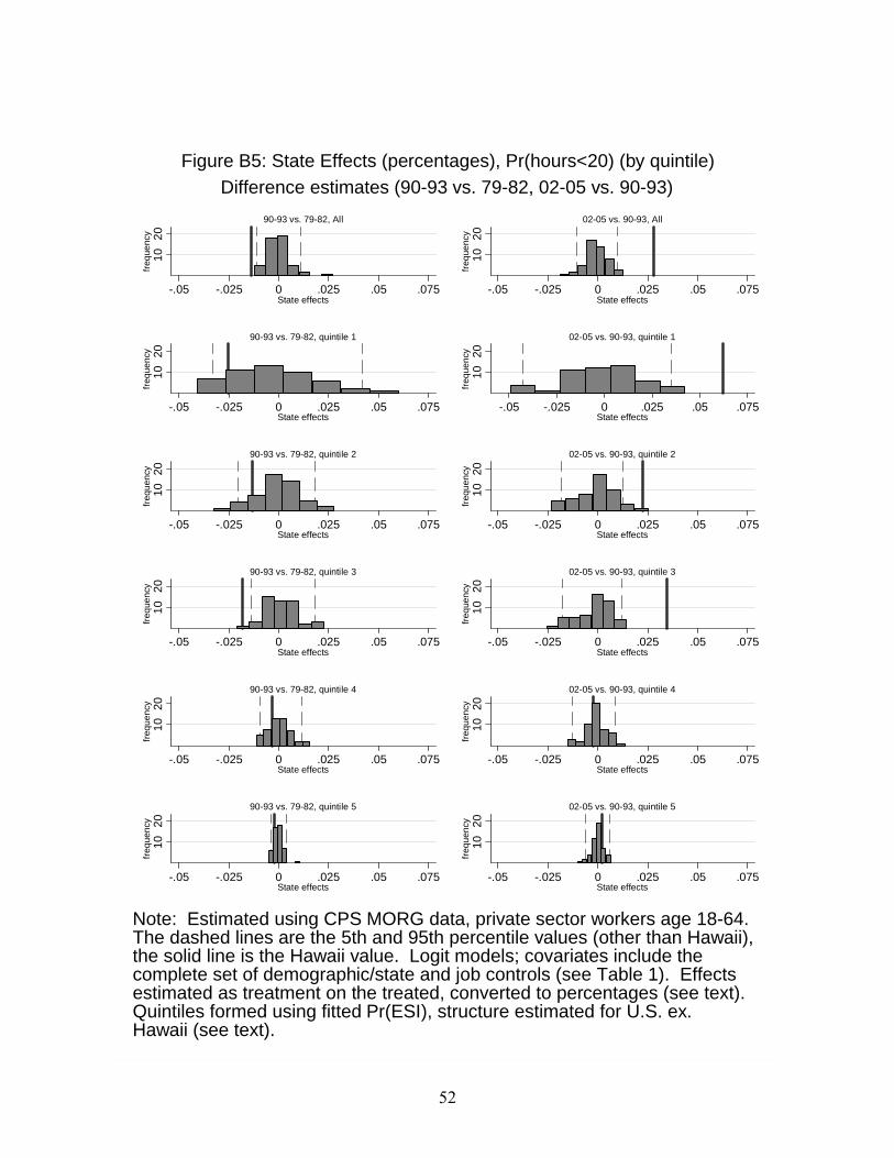
52

10

20

freq

uenc

y

-.05 -.025 0 .025 .05 .075State effects

90-93 vs. 79-82, All

10

20

freq

uenc

y

-.05 -.025 0 .025 .05 .075State effects

02-05 vs. 90-93, All

10

20fr

eque

ncy

-.05 -.025 0 .025 .05 .075State effects

90-93 vs. 79-82, quintile 1

10

20fr

eque

ncy

-.05 -.025 0 .025 .05 .075State effects

02-05 vs. 90-93, quintile 1

10

20fr

eque

ncy

-.05 -.025 0 .025 .05 .075State effects

90-93 vs. 79-82, quintile 2

10

20fr

eque

ncy

-.05 -.025 0 .025 .05 .075State effects

02-05 vs. 90-93, quintile 2

10

20fr

eque

ncy

-.05 -.025 0 .025 .05 .075State effects

90-93 vs. 79-82, quintile 3

10

20fr

eque

ncy

-.05 -.025 0 .025 .05 .075State effects

02-05 vs. 90-93, quintile 3

10

20fr

equ

ency

-.05 -.025 0 .025 .05 .075State effects

90-93 vs. 79-82, quintile 4

10

20fr

equ

ency

-.05 -.025 0 .025 .05 .075State effects

02-05 vs. 90-93, quintile 4

1020

freq

uen

cy

-.05 -.025 0 .025 .05 .075State effects

90-93 vs. 79-82, quintile 5

1020

freq

uen

cy

-.05 -.025 0 .025 .05 .075State effects

02-05 vs. 90-93, quintile 5

Note: Estimated using CPS MORG data, private sector workers age 18-64.The dashed lines are the 5th and 95th percentile values (other than Hawaii),the solid line is the Hawaii value. Logit models; covariates include thecomplete set of demographic/state and job controls (see Table 1). Effectsestimated as treatment on the treated, converted to percentages (see text).Quintiles formed using fitted Pr(ESI), structure estimated for U.S. ex.Hawaii (see text).

Difference estimates (90-93 vs. 79-82, 02-05 vs. 90-93)

Figure B5: State Effects (percentages), Pr(hours<20) (by quintile)

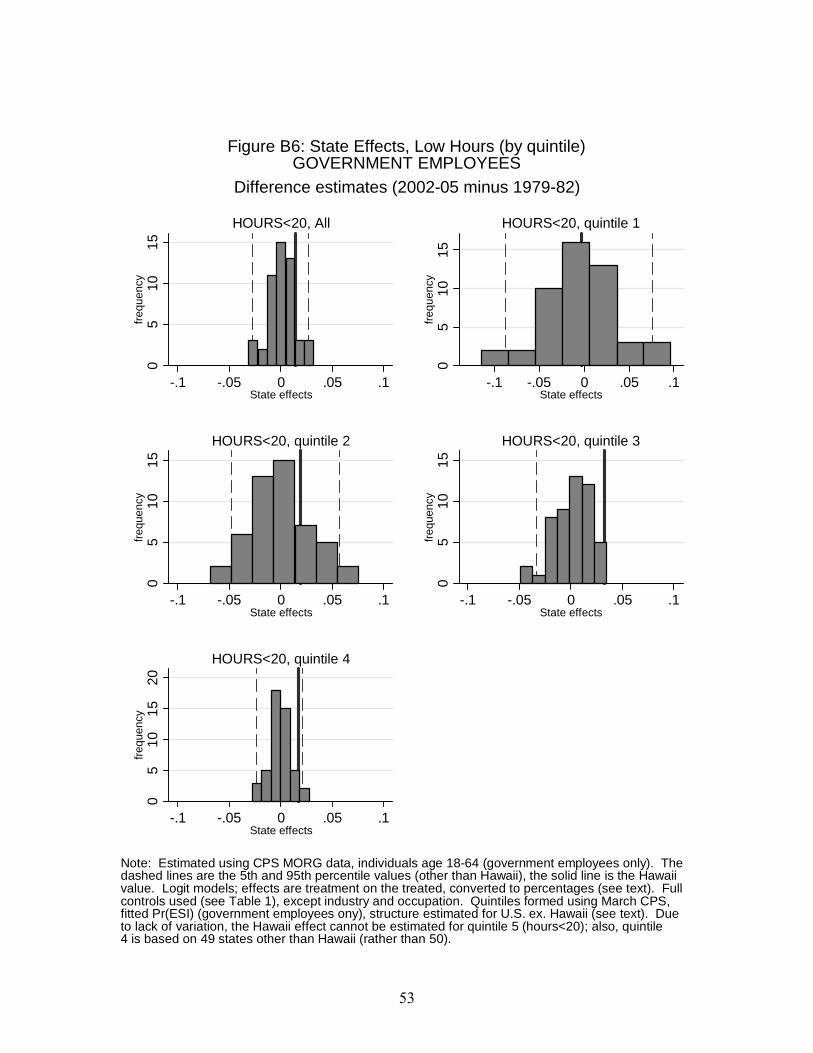
53

05

1015

freq

uenc

y


HOURS<20, All

05

1015

freq

uenc

y



05

1015

freq

uenc

y



510

15fr

eque

ncy



05

1015

20fr

eque

ncy



Note: Estimated using CPS MORG data, individuals age 18-64 (government employees only). Thedashed lines are the 5th and 95th percentile values (other than Hawaii), the solid line is the Hawaiivalue. Logit models; effects are treatment on the treated, converted to percentages (see text). Fullcontrols used (see Table 1), except industry and occupation. Quintiles formed using March CPS,fitted Pr(ESI) (government employees ony), structure estimated for U.S. ex. Hawaii (see text). Dueto lack of variation, the Hawaii effect cannot be estimated for quintile 5 (hours<20); also, quintile4 is based on 49 states other than Hawaii (rather than 50).


Figure B6: State Effects, Low Hours (by quintile)GOVERNMENT EMPLOYEES

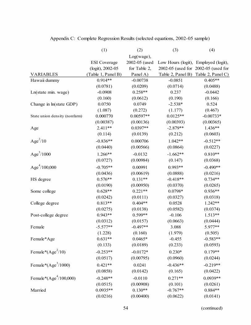
54

(1) (2) (3) (4)

VARIABLES

ESI Coverage (logit), 2002-05

(Table 1, Panel B)

Log(wage), 2002-05 (used

for Table 2, Panel A)

Low Hours (logit), 2002-05 (used for Table 2, Panel B)

Employed (logit), 2002-05 (used for Table 2, Panel C)

Hawaii dummy 0.914** -0.00738 -0.0851 0.405**(0.0781) (0.0209) (0.0714) (0.0488)

Ln(state min. wage) -0.0908 0.258** 0.237 -0.0442(0.160) (0.0612) (0.190) (0.166)

Change in ln(state GDP) 0.0750 0.0749 -2.538* 0.524(1.087) (0.272) (1.177) (0.467)

State union density (nonfarm) 0.000770 0.00597** 0.0125** -0.00733*(0.00387) (0.00136) (0.00393) (0.00365)

Age 2.411** 0.0397** -2.879** 1.436**(0.114) (0.0139) (0.212) (0.0603)

Age2/10 -0.836** 0.000706 1.042** -0.512**

(0.0440) (0.00566) (0.0864) (0.0227)

Age3/1000 1.266** -0.0132 -1.662** 0.810**

(0.0727) (0.00984) (0.147) (0.0368)

Age4/100,000 -0.705** 0.00991 0.993** -0.490**

(0.0436) (0.00619) (0.0888) (0.0216)HS degree 0.576** 0.131** -0.418** 0.734**

(0.0190) (0.00950) (0.0370) (0.0265)Some college 0.628** 0.221** 0.0798* 0.936**

(0.0242) (0.0111) (0.0327) (0.0318)College degree 0.813** 0.404** 0.0528 1.242**

(0.0275) (0.0138) (0.0582) (0.0374)Post-college degree 0.943** 0.599** -0.106 1.513**

(0.0312) (0.0157) (0.0663) (0.0444)Female -5.577** -0.497** 3.088 5.977**

(1.228) (0.160) (1.979) (0.505)Female*Age 0.631** 0.0465* -0.455 -0.583**

(0.133) (0.0189) (0.233) (0.0593)

Female*(Age2/10) -0.253** -0.0172* 0.230* 0.179**

(0.0517) (0.00795) (0.0960) (0.0244)

Female*(Age3/1000) 0.421** 0.0241 -0.436** -0.219**

(0.0858) (0.0142) (0.165) (0.0422)

Female*(Age4/100,000) -0.248** -0.0110 0.271** 0.0939**

(0.0515) (0.00908) (0.101) (0.0261)Married 0.0935** 0.130** -0.767** 0.884**

(0.0216) (0.00400) (0.0622) (0.0141)

(continued)

Appendix C: Complete Regression Results (selected equations, 2002-05 sample)

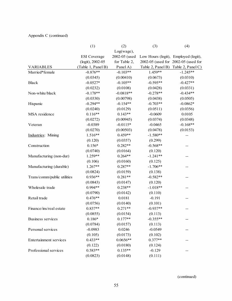
55

Appendix C (continued)

(1) (2) (3) (4)

VARIABLES


(Table 1, Panel B)





Married*female -0.876** -0.103** 1.459** -1.245**(0.0345) (0.00410) (0.0673) (0.0310)

Black -0.0527* -0.105** -0.595** -0.427**(0.0232) (0.0108) (0.0428) (0.0331)

Non-white/black -0.178** -0.0818** -0.278** -0.434**(0.0330) (0.00798) (0.0438) (0.0505)

Hispanic -0.294** -0.154** -0.703** -0.0862*(0.0240) (0.0129) (0.0511) (0.0356)

MSA residence 0.116** 0.143** -0.0609 0.0105(0.0272) (0.00945) (0.0374) (0.0348)

Veteran -0.0389 -0.0115* -0.0465 -0.168**(0.0270) (0.00503) (0.0478) (0.0153)

Industries: Mining 1.516** 0.459** -1.580** --(0.120) (0.0357) (0.299)

Construction 0.156* 0.282** -0.568** --(0.0740) (0.0164) (0.120)

Manufacturing (non-dur) 1.259** 0.264** -1.241** --(0.106) (0.0160) (0.125)

Manufacturing (durable) 1.267** 0.287** -1.706** --(0.0824) (0.0159) (0.138)

Trans/comm/public utilities 0.936** 0.281** -0.582** --(0.0843) (0.0147) (0.120)

Wholesale trade 0.994** 0.238** -1.018** --(0.0790) (0.0142) (0.110)

Retail trade 0.476** 0.0181 -0.191 --(0.0756) (0.0140) (0.101)

Finance/ins/real estate 0.837** 0.271** -0.937** --(0.0855) (0.0154) (0.113)

Business services 0.186* 0.177** -0.355** --(0.0784) (0.0157) (0.113)

Personal services -0.0983 0.0246 -0.0549 --(0.105) (0.0173) (0.102)

Entertainment services 0.433** 0.0656** 0.377** --(0.122) (0.0180) (0.124)

Professional services 0.583** 0.135** -0.129 --(0.0823) (0.0148) (0.111)

(continued)

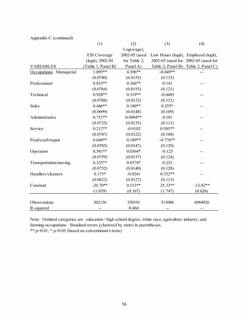
56

Appendix C (continued)(1) (2) (3) (4)

VARIABLES


(Table 1, Panel B)





Occupations: Managerial 1.095** 0.396** -0.849** --(0.0780) (0.0155) (0.133)

Professional 0.833** 0.366** 0.141 --(0.0764) (0.0155) (0.121)

Technical 0.928** 0.319** -0.0485 --(0.0788) (0.0132) (0.121)

Sales 0.446** 0.180** 0.255* --(0.0699) (0.0148) (0.109)

Administrative 0.751** 0.0904** 0.101 --(0.0735) (0.0135) (0.111)

Service 0.212** -0.0102 0.585** --(0.0747) (0.0122) (0.108)

Prod/craft/repair 0.640** 0.189** -0.776** --(0.0785) (0.0147) (0.129)

Operators 0.541** 0.0364* -0.125 --(0.0759) (0.0137) (0.124)

Transportation/moving 0.325** 0.0374* 0.232 --(0.0732) (0.0140) (0.128)

Handlers/cleaners 0.173* -0.0241 0.352** --(0.0822) (0.0127) (0.113)

Constant -26.70** 0.513** 25.33** -13.82**(1.059) (0.167) (1.747) (0.626)

Observations 302156 350191 513086 6984926R-squared -- 0.464 -- --

Note: Omitted categories are education <high school degree, white race, agriculture industry, and farming occupations. Standard errors (clustered by state) in parentheses.** p<0.01, * p<0.05 (based on conventional t-tests)

The Effect of an Employer Health Insurance Mandate on ... · The Effect of an Employer Health...

Documents

Transcript of The Effect of an Employer Health Insurance Mandate on ... · The Effect of an Employer Health...