The Economy of People’s Republic of China from 1953∗

Anton Cheremukhin, Mikhail Golosov, Sergei Guriev, Aleh Tsyvinski

March 29, 2014

Abstract

This paper studies structural transformation of the Chinese economy since 1953 througha lens of a two-sector growth model. We compute sectoral TFPs and wedges in the capital,labor, and product markets. This is a simple accounting procedure — given the wedges,the model matches the data exactly. Our first result is that the reduction in the labordistortion plays a key role in structural transformation in both the 1953-1978 and the1978-2011 period. The reduction of the labor distortion accounts for a half of the laborshare change in 1953-1978, almost all of the labor share change during the Great LeapForward, and 65 percent of the labor share change in 1978-2011. The reduction in thelabor distortion explains a half of GDP change during the Great Leap Forward and 1percent of the growth of GDP per year in 1978-2011. We further decompose the labordistortion in the wage wedge (the ratio of the sectoral nominal products of labor) and theprice wedge (the ratio of the relative price and the marginal rate of substitution). Wefind that the price wedge plays a dominant role in the sectoral labor change, on averagefour times as high as the wage wedge. The second set of the results is the quantitativeanalysis of the policies in 1953-1978. We find that the Great Leap Forward was a short-lived policy shock with welfare losses concentrated in one year but with an overall slightlypositive aggregate impact. Moreover, China’s development policies in 1953-1978 modeledto a large extent on the Soviet experience, significantly outperformed those during Stalin’sindustrialization. Our third result is to use the continuation of the 1953-1978 policies tomeasure the success and provide a benchmark for the post-1978 reforms. We find that theGDP growth would have been 2 percent per year lower, with higher distortions accountingfor 0.7 percent. The labor share would have been 27 percent higher, with higher labordistortions accounting for about 65 percent of the difference. Overall, we conclude thatchange in the intersectoral labor allocation distortion plays at least a role for the structuraltransformation in China as important as the change in the agricultural TFP emphasizedin the standard models of structural transformation, and that the wedge in prices ratherthan in the wedge in wages plays key role.

∗Cheremukhin: Federal Reserve Bank of Dallas; Golosov: Princeton and NES; Guriev: NES and SciencesPo; Tsyvinski: Yale. We are indebted to Carsten Holz for providing us with several data series in this paper andfor his many insightful discussions on Chinese statistics. We also thank Andrew Atkeson, Brent Neiman, LeeOhanian, and Stephen Roach for their comments and Stefano Malfitano and Kai Yan for research assistance.

“In 1949 a new stage was reached in the endeavors of successive Chinese elites to meet do-

mestic problems inherited from the Late Imperial era and to respond to the century-old challenge

posed by the industrialized West. A central government had now gained full control of the Chi-

nese mainland, thus achieving the national unity so long desired. Moreover, it was committed

for the first time to the overall modernization of the nation’s polity, economy, and society. The

history of the succeeding decades is of the most massive experiment in social engineering the

world has ever witnessed.” (Fairbank and MacFarquhar 1987, p. xiii)

1 Introduction

We study the Chinese economy from 1952, three years after the founding of the People’s Re-

public of China, through the lens of a two-sector neoclassical growth model. Our main focus

and the main contribution of the paper is the analysis of the 1953-1978 period.1 This “pre-

1978-reforms” period is important to study for several reasons. First, 1953-1978 was one of the

largest economic policy experiments and development programs in modern history. It is impor-

tant to evaluate the overall success or failure of this program as well as successes and failures of

the contributing factors and policies. Second, the successful First Five-Year Plan (FFYP), the

Great Leap Forward (GLF), and the post-1962 period of readjustment, recovery, and political

turmoil provide a range of interesting policies on their own. On one hand, the model of Chinese

development was based on Soviet Industrialization which we studied in Cheremukhin, Golosov,

Guriev, and Tsyvinski (2013). On the other hand, the Chinese policies were quite distinct from

their Soviet counterparts. We study a variety of questions using our model. What are the wel-

fare costs of the Great Leap Forward, and what were its main contributing elements? What if

China implemented the Soviet industrialization policies either starting with the First-Five Year

Plan in 1953, or with the Great Leap Forward in 1958? Thirdly, the analysis of the 1953-1978

period is perhaps the most important benchmark against which the post-1978 growth should

be measured. The main question here is how the Chinese economy would develop if the policies

of the 1953-1978 period continued. Relatedly, we provide a detailed analysis of the main factors

behind the 1978-2011 economic performance.

Specifically, our model is a two-sector (agricultural and non-agricultural) neo-classical model1Our analysis takes as an initial point the year of 1952 — after the Communist Party consolidated power

and launched a comprehensive modernization of economy and society. Coincidentally, this is also the start ofthe systematic collection of detailed economic statistics.

1

with frictions building on Cole and Ohanian (2004), Chari, Kehoe, McGrattan (2007) and

Chermukhin, et. al. (2013). The intratemporal labor distortion is the cost of intersectoral

reallocation of labor. The intratemporal capital distortion is the cost of intersectoral realloca-

tion of capital. We further decompose the intersectoral labor distortion in the wage wedge (the

ratio in the nominal sectoral products of labor) and the price wedge (the ratio of the relative

prices and the marginal rate of substitution). The intertemporal capital wedge is the cost of

reallocating capital across time. We further decompose the intersectoral capital distortion in

the interest rate wedge (the ratio in the nominal sectoral products of capital) and the price

wedge. Using a new constructed dataset covering 1952-2011 we then infer the wedges (and

other variables such as sectoral TFPs, government purchases, and international trade) from the

computed first order conditions of the model. We want to emphasize that the determination of

wedges is an accounting procedure. Given the wedges, the neoclassical model matches the data

exactly. In other words, the wedges are not calibrated but are determined to exactly match

the data. We provide an extensive discussion of the policies and historical evidence consistent

with the wedges that we find.

The first part of our analysis is to perform a wedge-accounting exercise for the whole period

of 1953-1978 to determine the main factors behind changes in the labor share, GDP, and

welfare. We fix wedges at their initial values (1953) for the whole period of interest (1953-78)

and simulate the economy. We then compare the simulated GDP, the labor share, and welfare

changes with the actual historical path. Compared to the counterfactual, welfare increases by

49.8 percent2, labor share is lower by 14.2 percent, and GDP growth is higher by 5.6 percent

per year. The growth of non-agricultural TFP contributed -8.5 percent, and the reduction of

labor distortion contributed -6.9 percent to the change in the labor share. Further decomposing

the labor distortion into the price wedge and the wage wedge we find that the former accounts

for -9.2 percent and the latter for 2.2 percent of the change in the labor share in agriculture.

The growth of non-agricultural TFP contributed 1.7 percent, the growth of agricultural TFP

contributed 0.8 percent, and the reduction of the labor barrier contributed 0.3 percent to the

annual growth of GDP. The same three factors are the largest contributors to the welfare change

during that period. While these are the numbers for the 1953-1978 period overall, changes in

the labor barrier played even more significant role in the GDP growth and the dominant role2The welfare numbers are reported in consumption equivalents, and in this case for generation born in 1953.

2

for changes in the labor share during the Great Leap Forward and the subsequent recovery.

The second part of our analysis is to assess the policies of the GLF, the FFYP, and the

1962-1978 period. We first simulate the economy assuming that the GLF did not happen. We

linearly extrapolate TFP in both sectors, the price wedge, the normalized capital and labor

wedges between 1957 and 1964. We find that the overall effect of the GLF on the welfare

of the consumer born in 1957 to be 2.6 percent of consumption. The most important factor

contributing to the change in the labor share (from peak to trough) is the reduction of the

labor distortion (-22 percent) with the sectoral TFP changes playing a minor role. Further

decomposing the labor distortion into the price wedge and the wage wedge we find that the

former accounts for -13.3 percent and the latter for 8.7 percent of the change in the labor share

in agriculture. The effect of the change in the labor distortion on GDP change is similarly large

(+22.8 percent) with +14.5 percent accounted by the price wedge but is counterbalanced by

the effects of the fall of TFP in non-agriculture (-14.7 percent) and agriculture (-6.5 percent).

It is also useful to consider changes in a year-by year welfare compared to the counterfactual.

Interestingly, the only year with a negative welfare effect of the GLF was 1960 (-3.9 percent).

The behavior of the wedges is consistent with the extensive overview of the policies and the

historical background that we provide. Overall, the GLF was a very short episode of disruption

to the economy with a negative welfare impact only in 19603. Summarizing, we find the

dominant role of the changes in the labor barrier for the structural transformation during the

Great Leap Forward.

We then perform two counterfactual simulations to compare China’s economic performance

and policies with those in the Soviet Union under Stalin. In the first comparison with the

Soviet Union, we start Stalin’s policies in 1957 (1956 is thus 1928 of Stalin’s policies) using

the wedges calculated in Cheremukhin et. al (2013). This choice of timing is guided by the

idea that the peak of the reforms in China under the Great Leap Forward (1960) should

coincide with Stalin’s peak of reforms (1932). This is done to isolate the GLF, and to highlight

striking similarities as well as differences between the GLF and the most intense phase of

Stalin’s collectivization. We find the overall effect on welfare of 3.9 percent of consumption.3It is important to emphasize that the welfare losses that we find for policies during the Great Leap Forward

are a lower bound. The representative consumer framework ignores the fact that different parts of populationbore very different consequences of economic policies (for example, it was the rural population that mainlysuffered famine). We also do not include the costs of political repressions. Taking these policies into account islikely to significantly increase welfare losses.

3

The overwhelmingly important factor for the difference in the labor share is the differences

in the labor barrier. While the price wedge behavior were strikingly similar in China and in

USSR, Stalin’s policies additionally succeeded in a dramatic decrease in the labor wedge. The

differences in GDP and welfare were accounted first by the much larger and permanent fall in

non-agricultural TFP in USSR contrasted with a smaller fall and a quick reversal in China and,

as a close second, by the differences in the labor barrier. We summarize the results as follows.

If China followed Soviet industrialization and collectivization policies, the results in terms of

welfare and GDP would have been worse but the labor share would have been significantly lower

than when it followed actual policies. The Great Leap Forward and Stalin’s collectivization

had similar negative effects on welfare at the peak of the campaigns. The quick reversal of the

policies under the Great Leap Forward led to a significantly higher labor barrier in China but

allowed to recover the losses in TFP. In contrast, Soviet collectivization policies implemented

in China would have achieved a long-term reduction of the labor barrier at the cost of a long-

term reduction of non-agricultural TFP. Again, we note the essential role played by the labor

barriers in comparison of these two policies.

Additionally, we contrast the combined effects of the FFYP and the GLF starting in 1953 to

Stalin’s collectivization and industrialization. This is done to compare the much milder initial

collectivization period of the very successful First-Five Year Plan together with the Great Leap

Forward to the much more brutal Soviet collectivization and industrialization. Specifically, we

impose the changes in wedges and sectoral TFPs calculated in Cheremukhin, et. al (2013) for

Stalin’s 1928-1939 economy on our model of the Chinese economy from 1953. Our main finding

is that Chinese policies in 1953-1964 led to significantly higher welfare (24.3 percent) compared

to Stalin’s policies in 1928-19394. The difference in the effects of the GLF versus collectivization

are very similar to the first comparison with the Soviet Union. However, China’s First Five-Year

Plan was indeed a very important success, especially, in its impact on non-agricultural TFP

(and also, albeit smaller, impact on agricultural TFP). In summary of these two comparisons

with the Soviet Union, China’s economic policies outperformed those in USSR.4One has to be careful with interpreting this comparison. By 1928, Soviet Russia recovered from the dis-

ruptions of the Civil War and also implemented a successful New Economic Policy Program (NEP). China,however, by 1953 might have still been in recovery from the Civil War. This may be one explanation for the fastTFP growth during the First Five Year Plan. Thus, we may overestimate the gains of our second comparison ofChina to USSR. However, the magnitude of the gain is large enough so that our main conclusion of the betterperformance of Chinese policies compared to Stalin’s policies remains.

4

We then study the 1978-2011 period through the lens of our model. We first perform

a wedge-accounting exercise for the 1978-2011 period. We fix wedges at their initial values

(1978) for the whole period of interest (1978-2011) and simulate the economy. We then compare

the simulated GDP growth, the labor share, welfare changes with the actual historical path.

Compared to the counterfactual, welfare increases by 99.1 percent, labor share is lower by

28.8 percent, and GDP growth is higher by 9.4 percent per year. The reduction of the labor

distortion contributed -19 percent to the change in the labor share and the growth of non-

agricultural TFP contributed -12.7 percent. Further decomposing the labor distortion into the

price wedge and the wage wedge we find that the former accounts for -14.9 percent and the

latter for -4.1 percent of the change in the labor share in agriculture. The growth of non-

agricultural TFP contributed 5.5 percent, the reduction of the labor distortion contributed 1

percent, and the the growth of agricultural TFP contributed 0.8 percent to the annual growth

of GDP. The same three factors are the largest contributors to the welfare change during that

period. Summarizing, the change in the labor barrier was the most significant factor for the

change in the labor share, the second largest factor in the growth of annual GDP, and had

almost as large impact on welfare as the agricultural TFP growth. It is useful to contrast our

results with Brandt, Hsieh, and Zhu (2008) and Dekle and Vandenbrouke (2012) who study

structural transformation of China post-1978 reforms. They find that the decrease in the barrier

to the labor reallocation played a relatively small role in the change in the labor share. The

key difference is that their notion of the barrier, the difference in the nominal wedges across

sectors, captures only a part of the labor distortion (that corresponds to our labor wedge but

omits the price wedge). When the reduction of the overall distortion is taken into account, as

we do here, the contribution of this factor increases almost fivefold. As such, our results are

closer to the conjecture of Young (2003) who argues that labor reallocation played a significant

role in the structural transformation in this period.

We then study what would happen if 1953-1978 policies continued after 1978. This is an

important counterfactual as it provides a benchmark against which to measure the success of

the post-1978 reforms. Specifically, we compare the actual data for the Chinese economy to the

simulated Chinese economy with 1953-1978 policies continued. We preserve the simulation for

the period 1952-1973, and impose the average trends in wedges and sectoral TFPs of 1953-1978

(excluding GLF) on the period 1974-2011. The most important result is that the average annual

5

GDP growth would be higher by 2 percent. The faster growth of the non-agricultural TFP

accounted for 0.8 percent, the faster reduction in labor and capital barriers (0.5 and 0.1 percent,

respectively) and in intertemporal capital wedge (0.1 percent) accounted for 0.7 percent, and

the faster growth of agricultural TFP accounted for 0.4. The reduction of labor distortion

played a dominant role (17.8 percent out of 27.3 percent) in the reduction of the labor share.

Further decomposing the labor distortion into the price wedge and the wage wedge we find that

the former accounts for -11.0 percent and the latter for -6.8 percent of the change in the labor

share in agriculture. In other words, the reduction in all wedges accounted for 35 percent of the

post-reform growth, while the reduction of the labor distortion accounted for 65 percent of the

change in the labor share. Summarizing, we conclude that the implementation of the post-1978

reforms in China led to a 2 percent increase in the annual GDP growth rates compared to the

continuation of the pre-1978 economy, and that the reduction of the distortions (and, most

importantly the labor distortion) played a very important role in the structural transformation

of the economy.

We now briefly discuss the state of the literature on the topic. Despite the importance of

the issue, there are no studies of the 1953-1978 period that use modern macroeconomic tools.

Ours is the first paper that analyzes this period from the point of view of the neoclassical

growth model, and provides a unified treatment of Chinese economy from 1953 to 2011. We

are aware of only one strand of papers dedicated to model-based macroeconomic analysis of

the 1953-1978 period by Gregory Chow (1985, 1993, 2002) whose work mainly focuses on data

issues. The post-1978 period received more attention from macroeconomists but perhaps less

prominence than its importance would suggest. Notable contributions are a collection of papers

in a landmark book edited by Brandt and Rawski (2008), an important quantitative analysis of

China’s post-1978 structural transformation and sectoral growth accounting by Brandt, Hsieh,

and Zhu (2008) and by Dekle and Vandenbroucke (2010, 2012), growth accounting by Young

(2003) and Zhu (2012), the model of “growing like China” with the focus on financial frictions

by Song, Storesletten, and Zilibotti (2011), and a model of misallocation by Hsieh and Klenow

(2010). We already commented on the key difference between our paper and Brandt, Hsieh,

and Zhu (2008) and Dekle and Vandenbroucke (2012) with regard to the notion of the labor

distortion and its consequentially significantly larger role in the structural transformation, and

in passing note that our model with wedges (by construction) matches the data exactly while

6

both of these papers rely on calibration to match some (but not all) features of the data.

More broadly, our paper is related to the studies of the the structural transformation as

Caselli and Coleman (2001), Konsagmut, Rebelo and Xie (2001), Stokey (2001), Ngai and

Pissarides (2007), Acemoglu and Guerrerie (2008), Buera and Kaboski (2009, 2012), Herrendorf,

Rogerson and Valentiniu (2013). The main difference with this literature is that we find that

the changes in the labor distortions (and policies associated with it) play an important role in

the structural transformation. Also notable is a two-sector model of growth accounting with

misallocation applied to Singapore by Fernald and Neiman (2010).

The paper is organized as follows. Section 2 develops the model and defines the wedges.

Section 3 describes the data and calibration. Section 4 calculates and describes the wedges and

provides an extensive overview of the policies and historical background consistent with the

wedges. Section 5 contains all the counterfactual simulations. Section 7 concludes.

2 Main Idea and Theoretical Framework

2.1 Model

We consider a standard two-sector neo-classical general equilibrium model in discrete time,

similar to the one we used to analyze Stalin’s industrialization (Cheremukhin et al., 2013).

There is an economy populated by Nt identical individuals. There are two sectors in the

economy, agricultural (A) and non-agricultural (M). In each period, t, output in sector i ∈

{A,M} is produced according to the Cobb-Douglas production function

Y it = F it

(Kit , N

it

)= Ait

(Kit

)αK,i(N it

)αN,i , (1)

where Ait, Kit , and N i

t are, respectively, total factor productivity, capital stock, and labor in

sector i; αK,i and αN,i satisfy αK,i + αN,i ≤ 1. We denote by F iK,t and FiN,t the derivatives of

F it with respect to Kit and N i

t .

Each individual maximizes discounted utility of consumption:

∞∑t=0

βtU(cAt , c

Mt

), (2)

where

U(cAt , c

Mt

)= η log

(cAt − γA

)+ (1− η) log cMt ,

7

cAt is consumption of agricultural goods and cMt is consumption of non-agricultural goods.5 The

subsistence consumption level of agricultural goods is denoted by γA ≥ 0. The discount factor

is β ∈ (0, 1). We use notation U ic,t to denote the derivative of U in period t with respect to the

consumption good i ∈ {A,M}.

Population growth is exogenous. The total population in period t is denoted by Nt. The

fraction of total labor allocated to agricultural and non-agricultural sector in period t are

denoted, respectively, by NAt +NM

t . Each working individual is endowed with one unit of labor

services which he supplies inelastically. The share of working age population χt is exogenous.

Therefore, the feasibility constraint for labor is

NAt +NM

t = χtNt, (3)

We assume that the new capital It can be produced only in the non-agricultural sector.

Capital can be used in any sector. Aggregate capital in period t is denoted by Kt. Capital

allocated in period t to agricultural and non-agricultural sector is denoted, respectively, by KAt

and KMt . The law of motion for aggregate capital is given by

Kt+1 = It + (1− δ)Kt, (4)

where δ is the depreciation rate. The capital is allocated to sectors according to

KAt +KM

t = Kt. (5)

We assume that there exists an exogenous sequence of government consumption of non-

agricultural goods, GMt . Let exAt and exMt denote net exports of agricultural and non-

agricultural goods in period t. Let qt be exogenous terms of trade for those goods.

The feasibility conditions in the two sectors are

NtcAt + exAt = Y A

t , (6)

and

NtcMt + exMt +GMt + It = YM

t . (7)5In the model, we use terms “non-agriculture” and “manufacturing” interchangeably. While construction

and services played a very important role in China’s industrialization, in this paper we focus on a two-sectormodel and aggregate all non-agricultural production into one sector. In the data, cMt corresponds to the privateconsumption of all non-agricultural goods and services.

8

Throughout the paper we assume that the trade balance is zero in all periods, so that the

net exports satisfy

qtexAt + exMt = 0. (8)

Given exogenous parameters and initial conditions (K), equations (2)-(8) provide a complete

description of our model.

2.2 First order conditions without frictions

We now characterize a standard social planner’s problem. The optimality conditions are as

follows:

the intratemporal capital allocation condition across sectors is

1 =UMc,t

UAc,t

FMK,t

FAK,t, (9)

the intratemporal labor allocation condition is

1 =UMc,t

UAc,t

FMN,t

FAN,t, (10)

and the intertemporal (Euler) condition is

1=(1 + FMK,t+1 − δ

)βUMc,t+1

UMc,t. (11)

The solution to this social planner’s problem coincides with the decentralized competitive equi-

librium. We omit the formal definition of the competitive equilibrium as it is standard. In the

competitive equilibrium, all agents pool their income and maximize their utility (2) subject to

a budget constraint in each period

pAt NtcAt +Ntc

Mt +KA

t+1 +KMt+1 =

= wAt NAt + wMt N

Mt +

(1 + rAt − δ

)KAt +

(1 + rMt − δ

)KMt + ΠM

t + ΠAt − Tt,

where wit, rit,Πit are, respectively, the wage, the rate of return on capital, and the profit in sector

i; pAt is the price of agricultural goods in terms of non-agricultural goods; and Tt is the lump

sum taxes.

Firms in sector i hire capital and labor to maximize profits

Πit = max{Ki

t ,Nit}pitA

it

(Kit

)αK,i(N it

)αN,i − witN it − ritKi

t ,

9

where pMt = 1.

Maximization behavior of the firms implies that wit and rit are equal to the marginal product

of capital and labor in sector i in each period. Maximization behavior of workers and owners of

capital implies that wit and rit are equalized across sectors. Maximization of utility by consumers

implies that

1 =UAc,t

pA,tUMc,t, (12)

We show that data rejects the implications of this frictionless competitive equilibrium.

2.3 Wedges accounting

The Chinese economy since 1950 had a large number of institutional frictions and government

policies that distorted decisions of households and firms. In order to map these frictions and

policies into distortions, we use the methodology developed by Cole and Ohanian (2004) and

Chari, Kehoe and McGrattan (2007) and applied in our paper to USSR (Cheremuknin, et. al.

2013).

Specifically, we define four wedges, each equal to deviations in the right hand side of equa-

tions (9), (10), (11), and (12) from 1. The first three wedges correspond to the intratemporal

distortions in capital and labor allocations between sectors and to the intertemporal distortion.

The fourth wedge is related to one of the main policies used by communist planners — price

scissors. This policy introduces a wedge between the relative prices that a producer of agri-

cultural goods faces, and the prices that consumers of agricultural goods pay. Specifically, if

producer of agricultural goods faces a price pA,t and a consumer faces a price p̃A,t, then the price

scissors wedge, 1 + τC,t, is given by 1 + τC,t = p̃A,t/pA,t =UAc,t

pA,tUMc,t. Thus, using additional data

on the producer relative prices (for the first three wedges), we define four wedges, τR,t, τW,t, τC,t

10

and τK,t+1 as follows

1 + τR,t ≡FMK,t

pA,tFAK,t=rMtrAt

, (13)

1 + τW,t =FMN,t

pA,tFAN,t=wMtwAt

,

1 + τC,t =UAc,t

pA,tUMc,t,

1 + τK,t+1=(1 + FMK,t+1 − δ

) βUMc,t+1

UMc,t.

Note that the intratemporal distortions for capital and labor implied by the right hand

side of expressions (9) and (10) are given by 1 + τ̃R,t = (1 + τR,t) / (1 + τC,t) and 1 + τ̃W,t =

(1 + τW,t) / (1 + τC,t). We call these two wedges a capital and a labor distortion, or normalized

capital and labor wedge. These normalized wedges (as well as the intertemporal wedge) do not

require knowledge of the prices.

The labor distortion, for example, implies that reduction in misallocation of labor between

agriculture and manufacturing can be achieved either by reducing the wedge τW,t, which is

determined by the ratio of the wages paid in the two sectors and in many models is often related

to the size of distortions to labor mobility or by increasing τC,t, which measures distortions

between consumer and producer prices. This distinction helps us to evaluate the effect of

different policies.

Finally, one can also think of{AMt , A

At , ex

it, G

Mt

}Tt=0

as wedges. These variables are exoge-

nous to the equilibrium and — as the wedges above — depend on the policies and institutional

frictions.

We want to emphasize that our analysis is essentially an accounting procedure. Given initial

K0, we find{AMt , A

At , τR,t, τW,t, τC,t, τK,t, ex

it, G

Mt

}Tt=0

such that the competitive general equi-

librium allocations with wedges{AMt , A

At , τR,t, τW,t, τC,t, τK,t, ex

it, G

Mt

}Tt=0

match data exactly.

This allows to compute the marginal contribution of each wedge to the deviations of data from

undistorted allocations and carry out quantitative analysis of various counterfactuals.

11

3 Data and calibration

In this section we discuss the construction of the data for a systematic analysis of the structural

transformation of the Chinese economy from 1952 to 2011. Most importantly, this section

details the procedure for constructing sectoral variables as well as defense spending, capital

series and international trade. To our knowledge, this construction of the data for this period

for an application of a two-sector neoclassical model is new.

3.1 Data sources and construction of the data

The main source of data on value added for the 1952-78 period is Hsueh and Li (1999), “China’s

national income 1952-1995” (HL). We use nominal value added by sector and the growth rate of

real value added by sector from HL to construct indices of real value added in the agricultural

(primary) sector and the non-agricultural (secondary and tertiary) sector in 1978 prices. The

same source allows us to estimate the relative prices of agricultural goods to non-agricultural

goods by taking the ratio of price deflators in the two sectors. The price deflator in each

sector is computed as the ratio of nominal to real value added in that sector. HL is also our

source for gross fixed capital formation in current prices which serves as our measure of nominal

investment. We convert it to real investment using the GDP deflator.

The second source of data on value added for the period of 1978-2011 is the China Statistical

Yearbook (2012) (CSY) provided to us by Carsten Holz. We apply the same method to the

data from the CSY to estimate real value added by sector, real aggregate investment and the

relative price of agricultural and non-agricultural goods.

We use Holz (2006), Tables 19 and 20 on pages 159-161, as our main source for aggregate

and sectoral capital stock. We use the level of capital and its ratio to GDP in 1953 to estimate

the initial level of capital in 1978 prices. We apply the perpetual inventory method (with

a depreciation rate of 5 percent) to our series for real investment in 1978 prices (computed

from CSY and HL) to obtain the series for aggregate capital in 1978 prices. The series that

we obtain is largely consistent with Holz’s estimates of aggregate capital stock for 1953-2006,

with two minor differences: Holz computes capital in constant 2000 prices and uses a variable

depreciation rate which ranges between 3 and 5 percent.

We also use data from Holz (2006) to divide the aggregate capital stock into capital used

12

in the agricultural and non-agricultural sectors. This sectoral division of capital stock is only

available for 1978-2011. For earlier years we use the data on sectoral investment from Chow

(1993) to estimate the composition of capital stock by sector. We use net capital stock accu-

mulation by sector from Table 5 on page 820 in Chow (1993), and then apply the perpetual

inventory method to accumulate sectoral capital stock for 1953-1978. As initial values we use

the value from the same table for non-agricultural capital, and the value of 450 for agricultural

capital. We then break down by sector the total real capital stock in 1978 prices computed

earlier using the relative proportions implied by Chow’s data.

We use data on the labor force and its composition from Holz (2006), Table 14 in the

appendix on page 238. We extrapolate it for the period 2003-2011 assuming a constant rate of

exit from the agricultural sector. We use data on population from the Palgrave International

Historical Statistics database and extrapolate values for the 2003-2011 period in the same way.

The data on defense spending comes from three main sources. The earlier period of 1952-

1995 is jointly covered by HL and CSY, which report nominal defense spending in yuan. For

the period 1983-2011 an alternative source of data is the website of the Stockholm International

Peace Research Institute (SIPRI) which reports spending on defense for a variety of countries

as a percent of GDP. For the overlapping period the trends are broadly consistent, but the

exact estimates vary by a factor of 1 to 1.5. As there seems to be no reliable way of obtaining

more precise estimates, we average the two available sources for the overlapping period. We

obtain an estimate of real defense spending in 1978 prices using the share of defense in GDP

from these two sources.

The main source for data on sectoral exports and imports is Fukao, Kiyota and Yue (2006)

(FKY). FKY report data on China’s exports and imports by commodity at the SITC-R 2-digit

level for 1952-1964 and for 1981-2000, obtained from the “China’s Long-Term International

Trade Statistics” database. Using data from FKY, we construct estimates of nominal exports

and imports of agricultural and non-agricultural commodities. We then subtract imports from

exports to obtain estimates of net exports by sector. We use the price deflators computed

earlier to estimate real net exports by sector in 1978 prices. For the 1965-1980 period, to our

knowledge, there is no available data on trade by sector. We linearly interpolate the ratios of

net export to value added by sector for this intermediate period. For the 2001-2011 period we

extrapolate these ratios using trends from 1995-2000.

13

We convert real GDP per capita in 1978 prices to 1990 international dollars using Maddison’s

estimate of 4803 dollars of 1990 per person for the year 2003. We then apply real GDP growth

rates (in constant 1978 prices) to construct real GDP per capita in international dollars for other

years in the 1952-2011 period. This series may differ slightly from real GDP in international

dollars reported by Maddison for other years, as relative prices changed. However, our index

captures well the general patterns and the long-term growth rates.

3.2 Summary of the data

Figures 1 and 2 show aggregate and sectoral, agricultural and non-agricultural, data for China

for 1952-2011. We subdivide the discussion of this period into two subperiods: pre- and post-

1978 reforms.

China 1952-1977

The Chinese economy in 1952-1977 grew rather rapidly, with a 3.9 percent average rate of

growth of real GDP per capita. However, the economy did not experience structural transfor-

mation from agriculture. The primary occupation for 83 percent of the working-age Chinese

population was agriculture in 1952, and this fraction declined very slowly (with the exception

of the brief period during the GLF when about 20 percent of the labor force was temporarily

moved from agriculture to manufacturing), remaining above 80 percent until 1970 and declining

to 75 percent in 1977. The role of agriculture in the economy was also very important, with

about 65 percent of value added produced in agriculture in 1952, declining only to 30 percent

in 1977 (with a similarly brief downward shift during the GLF). International trade was rather

insignificant – China’s net export of agricultural production was only 3 percent prior to the

GLF and declined to zero after 1960. The imports of non-agricultural goods constituted an

even smaller fraction of non-agricultural value added in the same period. Defense spending was

a large component of manufacturing production accounting for 6 percent of GDP.

China 1978-2011

In 1978-2011 growth in real GDP per capita increased to 8.4 percent annually. This coin-

cides with a rapid increase in investments (as a share of GDP) and reallocation of labor from

agriculture to non-agriculture. The share of labor force in agriculture fell from 75 percent in

1977 to 40 percent in 2011. The share of value added produced in the agricultural sector fell

from 30 percent to 5 percent respectively. Defense expenditures dropped abruptly from 6 per-

14

cent of GDP to 1.5 percent of GDP in the late 1980s. The relative prices of non-agricultural

goods show a 40-percent appreciation in the 5 years following the reforms, and then continued

appreciating at approximately the same pace as in the pre-reform period.

Figure 2 shows agricultural and non-agricultural per capita value added in 1978 prices,

capital stock, and government expenditures. Non-agricultural value added shows remarkable

growth throughout both periods, growing at 8.7 and 10.3 percent, respectively. Agricultural

value added grew much slower, at 2.8 percent prior to reforms, and 4.1 percent afterwards. The

ratios of sectoral capital stock to sectoral GDP remain roughly stable over the whole period.

Figure 1: Macroeconomic indicators of the People’s Republic of China, 1952-2011.

3.3 Calibration

To calibrate the model we need to choose the values of eight parameters and the initial value

of capital stock. The five technology parameters include the elasticities of production functions

in the agricultural and manufacturing sectors with regard to capital and labor, (αKi, αNi),

and the depreciation rate, δ. Three preference parameters include the discount factor, β, the

asymptotic agricultural consumption share, η, and the subsistence level in agriculture, γA.

The depreciation rate is set to δ = 0.05, and the discount factor is set to β = 0.96.

The asymptotic consumption shares of agricultural and non-agricultural goods are set to η =

15

Figure 2: Macroeconomic indicators of People’s Republic of China, 1952-2011.

0.15 and 1 − η = 0.85, correspondingly.6 We assume that all intermediate goods used in the

production of manufactured goods represent labor. We set the corresponding factor shares

for the manufacturing sector to αK,M = 0.3 and αN,M = 0.7. Instead, we assume that all

intermediate goods used in the production of agricultural goods represent land. We set the

remaining capital and labor shares to αK,A = 0.14 and αN,A = 0.55 (thus assuming that land’s

elasticity is 1-0.14-0.55=0.31). The values for these parameters are also in the range of values

adopted by Caselli and Coleman (2001) and Stokey (2001) and calibrated using direct estimates

for the U.S. and the U.K.7

The elasticities for the agricultural sector are also in line with estimates of Tang (1982),

who has the contributions of labor, capital and land at 0.5, 0.1 and 0.25 respectively, with the

remaining share of 0.15 assigned to intermediate inputs. However, there is a large variation in

estimates of factor shares in Chinese agriculture in the literature, neatly summarized by Wen

(1993, Table 9, page 27). We check the robustness of our results to these alternative estimates

of factor shares in an online appendix.6Parameter η only enters as a constant in one first-order condition and determines the scale of the price

wedge, τC,t. By the same token, since the relative price of agricultural to manufacturing goods is measured inthe data as an index, the scale of the price wedge, τC,t, means little, so we normalize it to be zero in 1952.

7Caselli and Coleman (2001) use the values αK,M = 0.6, αN,M = 0.34, αK,A = 0.21 and αN,A = 0.6. Stokeycalibrates αK,M = 0.5, αN,M = 0.5, αK,A = 0.17 and αN,A = 0.38.

16

We choose the initial capital stock to match the observed level of capital in 1952. We do not

have data needed to directly determine the subsistence parameter, γA. We set the subsistence

level to 56 yuan per capita per year in 1978 prices. This subsistence level accounts for 66

percent of agricultural consumption per capita in 1952. If we set it higher than 79 percent

of consumption of 1952, the simulated economy would go below the subsistence level in 1960

during the famine of the Great Leap Forward. We explore in an online appendix, how our main

results change in response to alternative calibrations of γA. Finally, for χt, the path of the

fraction of labor force in the population is pinned down by the data.

We provide extensive robustness checks for all key parameters in the online appendix.

4 Wedges and policies

We now proceed with the calibrated model to compute wedges using equations (13). Figure 3

shows wedges for China with solid lines and their average level (or trends, for the case of TFPs)

with dashed lines. In this figure, we draw the trends for the pre-reform (1953-1978) and for the

post-reform (post-1978) periods. This division is consistent with the common historical view

and with the related evidence for the structural break in 1978.

In the remaining part of the section, we give a more nuanced division in sub-periods.

Before starting the analysis of the wedges, it is useful to establish the periodization of the

PRC economic history. Naughton (2007) considers Economic Recovery (1949-52), the Twin

Peaks of the First Five-Year Plan (1953-1956), Great Leap Forward (1958-1960), Crisis and

“Readjustment” (1961-1963), Launch of the Third Front (1964-66), the Cultural Revolution

(1967-69), the Maoist Model: a New Leap (1970-1972), Consolidation and Drift (1972-76), and

the Leap Outward and end of Maoism (1978-). Cambridge History of China (MacFarquhar

and Fairbank 1987, Perkins 1991) considers the periodisation as follows: Emulating the Soviet

Model (1949-57) with three subperiods – Consolidation and Reconstruction (1949-52), Socialist

Construction and Transformation (1953-56), Adjusting the New Socialist System (1956-57);

the Search for a Chinese Road (1958-65) – with two subperiods Great Leap Forward (1958-

62) and Economic Recovery (1963-65); and the 1966-82 period with the following subperiods

– Disruption in the economy (1966-69), Industrial development strategy (1966-76), Changing

industrial strategies (1977—80), Accelerating industrial growth, 1982—1987. Selden (1979,

p.153) provides an exceptionally useful summary of the main stages in China’s development

17

priorities.

Figure 3: China: Wedges

In what follows, we consider a periodization into the First Five-Year Plan (1952-57), Great

Leap Forward (1958-62), the period of 1962-78, and the post-reform period of 1978 onward.

We stop at 2011 and do not discuss the reforms proposed in the Third Plenum in November

2013.

4.1 Initial conditions

We begin with briefly discussing the initial conditions and decisions and strategies chosen in

1949-52. The creation of the People’s Republic of China in 1949 was a turning point in Chinese

history. After the World War II and the Civil War, the Communist party consolidated power

and embarked on a comprehensive political, economic and social transformation. Following the

Soviet experience, the Chinese communists planned to turn a backward agrarian economy into

a modern industrial power through collectivization of agriculture, expropriation of agricultural

surplus, and a massive top-down industrial investment.

The initial conditions in China 1950 were different from those in the Soviet Union. Imperial

Russia was behind its Western counterparts, yet, it had been growing for several decades before

the World War I. Stalin inherited a relatively developed industry and urbanized population.

The Chinese economy before 1950 was a stagnating agrarian one. It had not experienced

18

growth; moreover, its very institutions were built to preserve the status quo rather than to

promote growth. “The Confucian political economy . . . was that of an agrarian empire and

was directed above all to the maintenance of social stability through the guarantee of minimal

standards of survival and the amelioration of unacceptable inequalities.” (Richardson, 1999, p.

85). Lin (2012, p. 32-34) also argues that the tradition of the Chinese bureaucratic state was

to reject the modern (or Western) approach to innovation thus creating a bias for the status

quo. The second important distinction was land scarcity. While in Russia, especially after the

World War I and the Civil War of 1917-22, labor was relatively scarce compared to land, in

China, the combination of centuries of stagnation and of rapid population growth8 resulted in

relative labor abundance and land scarcity.

Despite the difference in the initial conditions, the Communist Party immediately an-

nounced a program that was very similar to the Soviet model (see Lin, 2012, p. 75, Spence,

2013, p. 461 on the Common Program for China announced at the People’s Political Consulta-

tive Conference convened by Mao Zedong in September 1949). An ambitious plan was created

for rural reform through rent reduction and land redistribution based on the Soviet model; and

the work centered on the rehabilitation and development of the heavy industry.

By 1952, the communist government completed the initial post-war recovery: inflation had

been brought under control, output in both industry and agriculture surpassed the highest

pre-war levels. (Naughton, 2007, p. 64, Richardson, 1999, p. 103). At the very same time, the

government completed a massive redistribution of land from rich to poor households: about 43

percent of China’s cultivated land was redistributed to about 60 percent of the rural population

(Teiwes, p. 87). This redistribution was brutal: according to Spence (2013, p. 463), one

landlord family in six had a member killed during the land reform; a total of about 1 million

people who died. The redistribution to the poor also included massive investment in public

health (Perkins 1975, p. 127). By 1952, the government also introduced systematic collection

of economic data (Richardson, 1999, p. 25, Rawski, 1979, p.15, Perkins, 1975, p. 116).

4.2 Wedges in 1952-1957 (First Five-Year Plan)

The period of 1952-57 was that of the First Five-Year Plan, “an unusually successful program of

economic development” (Lardy 1987a, p.157). The plan was modeled on the Soviet experience8The population of China increased from 30 million in 1800 to 600 million in 1950 (Richardson, 1995, p. 2).

19

of collectivization and industrialization in 1928-1939: the development program was drawn

“half in Moscow, half in Peking” (Naughton 2007, p. 66), and the principal slogan was “Let’s be

modern and Soviet” (Selden 1979, p.153). On the other hand, there was a much more moderate

attitude towards agriculture than the abrupt Soviet change9. China’s planners – who learned

from the USSR and who also understood that agriculture was much more important for China

– never tried to sacrifice agriculture as badly (Perkins 1975, p. 143). China proceeded with

collectivization much more gradually.10 There was no single-minded focus on the expropriation

of the agricultural surplus. The rich peasants were restricted but not liquidated. (Teiwes, p.

110). This made China’s First Five Year Plan much more successful than its Soviet counterpart

(Lardy, p. 155).

We now turn to Figure 3 to document the behavior of the wedges and to provide the

historical background that is consistent with the wedges.

Sectoral TFPs grew significantly. Average annual TFP growth was 4.3 percent between

1952 and 1957 in agriculture, and by 7.8 percent in non-agriculture.

The growth of TFP in non-agriculture is consistent with several facts. First, Soviet assis-

tance played an important role. Lardy (1987a, p. 178) argues that Soviet technical assistance

was “unprecedented in the history of the transfer of technology” as China “received the most

advanced technology available within the Soviet Union, and in some cases this was the best

in the world”. Close to 6000 Soviet advisors helped establish and operate the 156 large-scale

capital intensive Soviet-assisted projects (Naughton 2007, p. 66; Rawski, 1979, p. 51)11. These

projects constituted “the core of the industrialization program” and absorbed about a half of

total industrial investment (Lardy 1987a, p. 158). Eckstein (1977, p. 102) considers these large

turnkey industrial installations designed in Russia, transported in full to China, installed and

often operated by Soviet advisors as one of the “crucial element[s] of industrialization of China9As evidenced, for example, in Mao’s famous Speech to the Political Bureau of the Central Committee, April

25, 1956 “On the Ten Major Relationships” which was the synthesis and perhaps the most important Mao’sstatement on a distinct approach China’s development and the first serious criticism of Soviet developmentstrategy (Selden 1979, p. 315-322).

10Mao was always “walking on two legs”, he was a Marxist but also wanted to adopt it to Chinese tradition(Schram, p. 1, p. 42-43).

11Li Fuchun, then the Chairperson of the State Planning Committee in the “Report on the First Five-YearPlan for Development of the National Economy of the People’s Republic of China in 1953-1957, July 5 and 6,1955” summarized: “We must center our main efforts on industrial construction ..., the core of which are the156 projects which the Soviet Union is designing for us, and which will lay out the preliminary groundwork forChina’s socialist industries” (Selden 1979, p. 296-7).

20

during the First Five-Year Plan”. The system of planning and development was itself modeled

on the Soviet Union and assisted by the advisors. Second and related to the first factor, the

import of the capital intensive goods and machinery (also to a large extent from USSR) played

an important role in allowing the economy to operate the “frontier technology” (Naughton 2007,

p.66). Eckstein (1977, p. 235) argues that import constituted as much as 40 percent of the

equipment component of investment in the 1950s. Third, the First Five-Year plan model was

a very technocratic approach that “paid considerable attention to complementarities, input-

output relations, and technical requirements in production and enterprise management” . The

management model placed great responsibilities on a director of enterprises, valued and utilized

technical experts, and provided some stratification in pay and benefits to improve incentives.

(Eckstein 1977, p. 89-90). The plan also stressed individual material incentives (Selden 1979,

p. 153). Overall, by the mid-1950s, modern technology was adopted on a large scale in industry

(Lardy 1987a, p. 144).12

The growth of TFP in agriculture is consistent with several facts. First, and unlike the Soviet

Union under Stalin, agriculture was never viewed purely as a source of revenue extraction for

the forced industrialization. Rural population was historically an important power base for the

Communist Party. Agriculture was also viewed as an important source of raw materials for the

industry. Overall, the process of collectivization in China was able to “limit the disorder and

destruction of economic resources that marked the Soviet comparing” (Teiwes 1987, p.141). We

return to this issue in a more detailed comparison with Stalin’s industrialization in Section 5.1.3.

Second, more efficient methods of agricultural production were implemented. Nolan (1976) gives

detailed figures and determines five such methods: (1) increase in irrigated areas; (2) increased

multiple cropping; (3) afforestation; (4) improved seeds; (5) increased collection and application

of organic fertilizers (see also Naughton 2007, Chapter 11). Thirdly, the collectivization led to

consolidation in the land plots that led to improvement in labor productivity, decreased the

travel time between plots, and allowed the use of mechanization (Spence 2013, p. 491)

The capital wedge decreased significantly. This is consistent with the main strategy of the

First Five-Year Plan that placed the overwhelming priority in allocation of investment resources

to industry and production of capital goods. Selden (1979, p. 153) states that the order of12Another factor that affected TFP in both the agricultural and the non-agricultural sectors of the economy

is the advances in basic hygiene, disease, and pest control that affected productivity and longevity (see, e.g.Spence 2013, p. 488).

21

economic priorities for that period was: heavy industry, light industry, agriculture. Lardy

(1987a, p. 158) and Eckstein (1977, p. 188) give details of investment allocation to industry

and agriculture to also argue about the low priority of agricultural investment.13

There is a slight increase in the price wedge starting in 1957. The First Five-Year Plan

laid the foundation of the government procurement at artificially low prices14 but certainly was

much more gradual and not to the extent of the Great Leap Forward or Stalin’s collectivization.

The magnitude of the increase in the price wedge is not surprising given the relative mildness

of the policies compared to the increase during the Great Leap Forward or during Stalin’s

collectivization.

There is an increase in the labor barrier starting in 1955. This is consistent with the start

of the implementation of the hukou system of registration of urban and rural population and

the restrictions on their movement. Cheng and Selden (1994) give a detailed account of the

origins of this system. The origins of the system can be be traced back to the 16th of July 1951

when the Ministry of Public Security issued “Regulations Governing the Urban Population”. At

that stage, the system was just a registration system. On 12 March 1954, the Ministry of the

Interior and Ministry of Labour issued an important “Joint Directive to Control Blind Influx

of Peasants into Cities” that was aimed at the cities and started to curb migration. Finally,

in 1954-1956 a set of measures was introduced to further limit and disincentivize migration

including, importantly, food rationing. While the hukou system and migration controls were

still in the incipient stage and far from the scope and strictness of the later years, the evidence

is consistent with the increase in the labor wedge starting from mid-1950s.15

In this and other subsections, we do not to focus on the the investment wedge. The primary

reason is that the investment wedge exhibits large short term fluctuations. This is consistent

with the large and frequent policy changes regarding investment but would necessitate a much

finer periodization of the economy, essentially, year by year.13The report by Li Fuchun gives the following state investment priorities: industrial departments – 58.2 percent

of total; agriculture – 7.6 percent; transport, post and telecommunications – 19.2 percent; trade, banking, andstockpiling – 3 percent; urban public utilities – 3.7 percent (cited in Selden 1979, p. 296-7).

14See, e.g., a detailed description in Eckstein (1977, p. 78 and p. 117 ) and Naughton (2007, p. 80).15Nolan and White (2007) also argue that the measures to control migration started to be effective after 1955.

For a longer history of hukou system see Chan and Zhang (1999).

22

4.3 Wedges in 1958-1962 (Great Leap Forward)

We now discuss the behavior of the wedges and sectoral TFPs during the Great Leap Forward

in Figure 3 and the policies and historical background consistent with these wedges. We also

use the calculation of the wedges and the connection of wedges to policies to argue in Section

5.1.3 that the GLF was even more drastic in some dimensions than Stalin’s Big Push.

The collectivization of agriculture was completed already by 1956: 98 percent of farm

households were members of cooperatives or collective farms (Naughton, 2007, p. 67). At

the same time, it was clear that the cooperatives failed — because of the lack of incentives

to exert effort and poor management and coordination (Naughton, 2007, p. 237, Spence,

2013, p. 509). The worrisome developments in agriculture resulted in a retrenchment. The

Eighth Party Congress (September 1956) discussed economic moderation; the earlier policies

were criticized as a “reckless advance”. Mao encouraged open debate and praised blooming

of the “Hundred Flowers”. However, already in 1957 Mao understood that freer debate may

be politically costly and changed his mind. He launched the “Anti-Rightist Campaign” that

targeted non-party intellectuals who had spoken out during the “Hundred Flowers”. About 800

000 were removed from their jobs, condemned and sent to labor camps (Naughton, 2007, 69).

Instead, Mao suggested to address the problem of falling agricultural output through a Great

Leap Forward. Instead of cooperatives (which included about 50 households), GLF introduced

communes (thousands of households). The communes would be used to mobilize resources

for construction, provide social services, and develop small-scale rural industries. Within the

communes, all material incentives were abolished. “These communes attempted to practice full

communism” (Rawski, 1979, p. 76.).

The reported results of 1958 were very positive. Partially, it was due to an exceptionally

good harvest, but falsification of reports by those who did not want to disappoint the author-

ities also played a role. “Evidently dazzled by claims that rural production under commune

management had doubled, increased tenfold, or even “scores of time”, the Central Committee

issued the ecstatic vision of the Great Leap forward” (Spence, 2013, p. 518). This resulted in

higher grain procurement quotas and higher targets of rural industrial production (notorious

“backyard furnaces”). At the same time, the complete destruction of incentives as well as poor

harvests had a dramatic negative effect on agricultural output. “In 1959, grain output declined

23

by 15 percent, in 1960 by another 15 percent, and in 1961 on par with 1960.” (Lin, 2012, p. 88).

The number of hogs in 1961 after private agricultural activity had been virtually eliminated

was only 52 percent of the 1957 peak.” (Perkins, 1991, p. 483). The combination of high plans

(and therefore procurement quota) and low output resulted in a great famine which cost about

30 million lives (Meng et al., 2013).

We find that TFP in agriculture fell by 50 percent from its peak in 1958 to the trough in

1962. TFP in manufacturing fell in 1958 by 33 percent and again in 1961 by 23 percent.

Several factors affected TFP in both manufacturing and agriculture in the first years of

GLF: rejection of material incentives, monetary rewards, bonuses in the industry, curtailment

of free markets in the countryside and the productive private farming plots – all of which

worsened incentives (Naughton 2007, p. 69; Lardy 1987b, p. 365).

The fall in TFP in agriculture is consistent with several factors. One factor was that pro-

ductivity fell due to poor management of agriculture under the commune system.16 Communes

that comprised over 5000 members became a predominant form of organization in agriculture,

and due to their size and organization were very difficult to effectively manage. Considering

the negative productivity impact of the communes Lardy (1987b, p. 370) argues that the most

important factor was in the construction and design of the irrigation projects which reduced

rather than raised yields. The unusually bad weather in 1960 also had serious adverse effects on

the yields.17 Li and Yang (2005) argue that the most important causal factors in the collapse of

agricultural output between 1958 and 1961 are: (1) the diversion of resources from agriculture,

which was responsible for 33 percent of the decline; (2) excessive procurement of grain affecting

physical strength of the peasantry accounting for 28.3 percent; (3) bad weather contributing

12.9 percent to the collapse.

The fall in productivity was reversed only after 1962. Following the agricultural crisis, the

state undertook the “Agriculture first” strategy. This strategy included reopening of private

plots (Lardy 1987b, p. 389), decentralization of commune management that essentially de-

creased the size of the production unit to that in 1955-56, and a greater reliance on material16Lin (1990) discusses a variety of hypotheses and presents a view emphasizing the role of incentives in the

fall of productivity.17See e.g. Selden (1979, p. 97) or a more recent study based on the meteorological data (Kueh 1995). The low

agricultural output was further exacerbated by miscalculation in the 1959 plan to reduce the area and resourcesallocated to grain production. This decision followed the successful harvest of 1958 and was done under thefalse supposition of the new era of significantly increased productivity in agriculture and following the massivefalsification of data on yields (Naughton 2007, p. 70)

24

incentives (Eckstein, 1977 p. 60-61).

The fall in manufacturing TFP is consistent with several factors. First, the collapse of

agricultural production led to severe shortage of agricultural materials for textile and food-

processing industries. Second, many small scale plants such as backyard steel furnaces were

extremely inefficient (e.g., Ekstein, 1977, p. 124).18 Third, the Sino-Soviet split led to the

departure of virtually all Soviet advisors in the late summer and early fall of 1960. This meant

that a large number of capital-goods projects had to be suspended (Eckstein, 1977, p.203;

Selden 1979, p. 97).

The reversal of the TFP fall after 1961 is consistent with the general “readjustment and

consolidation” policies that refocused industrial production to more specific and high produc-

tivity projects (e.g., petrochemical and fertilizer) rather than advancing on a broad front, and

to a revival of material incentives (Eckstein, 1977 p. 126).

The price wedge dramatically increased by a factor of 4.7 from 1958 to reach its peak in 1960,

before falling to the pre-GLF level in 1964. The level of state procurement of grain reached its

peak in 1959 and rural retentions per capita reached the trough in 1960 (Lardy 1987b, p. 381

Table 7; Li and Yang 2006, Table 1). Following the agricultural crisis, first attempts to scale

back procurement were evidenced in 1961. Also, in the winter of 1961, the fixed procurement

prices were raised (Lardy 1987b, p. 385). In 1962, procurement was drastically reduced (Lardy

1987b, p. 388).

The labor barrier dramatically decreased by 82 percent from 1957 to 1960 and then shot

back up returning to its 1957 level in 1964. It is not surprising that this was accompanied

by an unprecedented increase in the agricultural labor force.19 The reversal of the barrier is

consistent with the massive forced resettlement of urban population to the countryside. In

1961-62, about 30 million urbanites were thus moved to the countryside (Lardy 1987b, p. 387).

The capital barrier decreased dramatically to the trough in 1960 and then started its gradual

reversal. This behavior is consistent with several facts. The first years of the GLF strategy

were based on a massive infusion of capital both to the industries developed in the First-18Selden (1979, p. 100) gives the following estimates for these furnaces. In July 1958, there were 30-50

thousand small furnaces, in October – close to 1 million. By October 1960, only over 3000 were still operational,and the rest shut down. He further quotes an editorial from People’s Daily of August 1, 1959: “We must facethe problem frankly: Last year’s small furnaces could not produce iron”.

19In 1958, the number of workers state non-agricultural units rose by almost 21 million, an increase of 85percent compared with 1957. The peak level of employment in state units was 50.44 million at the end of 1960,more than double the number in 1957 (Lardy 1987b, p. 369)

25

Five Year plan, and importantly to small-scale industrial plants such as “backyard furnaces”

(Lardy 1987b, p.365)20. The reversal of the barrier afterwards is consistent with several facts.

There was a massive closure of the construction of industrial projects after the disastrous

first years of the GLF (Lardy 1987b, p. 387) and a corresponding increase in investment

allocated to agriculture. The “Agriculture first” strategy most significantly increased chemical

fertilizer production, electricity allocation, and the production of small agricultural implements

(Eckstein, 1977, p.60). These measures also are consistent with the increase in agricultural

TFP in those years.21

4.4 Wedges 1962-1978

The period of 1962-1966 was a period of recovery from the disaster of the Great Leap Forward

which we already started to discuss in the previous section. In 1962, the government backtracked

by reducing the size of communes to “production teams” of about 20-30 households per team.

(Lin, 2012, p. 89, p. 153.). Material incentives were reintroduced. 20 million workers were

sent back from cities to the countryside. Mao recognized that “backyard furnaces” were a

mistake (Mao Tse-tung, “Speech at the Lushan Conference,” 23 July 1959, in Stuart Schram,

ed. “Chairman Mao talks to the people,” 142-43, cited by Perkins, 1991, p. 478). These policies

continued throughout the Cultural Revolution, the last years of Mao and the first post-Mao

years — until the beginning of reforms in 1978. (Perkins, 1991, p. 486) The planning and Big

Push ideology persisted but was softer and less brutal than in the 1950s.

Agricultural TFP grew by 42 percent from the low of 1962 to the peak of 1966, but was

still 14 percent below the peak of 1958. The price wedge continued to decrease to reach its

trough in 1966. Both the increase in agricultural TFP and the decrease in the price wedge

are consistent with the continuation of the “readjustment and recovery” policy in agriculture.

Manufacturing TFP grew quickly — recovered to the pre-crisis peak of 1957 in 1964, and

increased by almost 60 percent from the low of 1961 to the peak of 1966. Both the growth of

manufacturing TFP and the rapidly increased capital wedge are consistent with the arguments20While often the first years of the Great Leap Forward are associated with the small scale projects such as

backyard furnaces (see, e.g. discussion in Spence 2013, p.), Lardy (1987b, p. 367) gives detailed statistics onthe preponderance of investment allocation to the medium and large-scale industrial plants.

21For example, special allocations of materials to produce small implements such as hand tools and carts wereimplemented in 1962, and the availability of these items was restored to the pre-GLF years (Lardy 1987b, p.391).

26

that the period of readjustment did not mean that fundamentally the growth strategy shifted

to prioritize agriculture. Rather, the moderates in the government – Zhou Enlai and Chen

Yun, among others – were successful in extending the period of readjustment until 1965 and in

deferring the Third Five-Year plan until 1966. In particular, they won in a critical debate on

the target for steel production, and were able to scale it down. However, the moderates only

slightly and temporarily altered the growth strategy of the primacy of the industrialization to

allow a respite with “agriculture first”. (Lardy 1987b, p. 396)22. The rapid increase in the

capital wedge is also consistent with the program of the “Third Front”. Mao worried about

US involvement in Vietnam and about the rift with the Soviet Union that potentially could

lead to a war. The “Third Front” was a massive construction program in the inland provinces

of the entire industrial base that would not be vulnerable to the attacks by the Soviets or

Americans.23 The Third Front was important even during the Cultural Revolution, but the

rapid expansion of the first phase was stopped by the Cultural Revolution. The labor wedge

continued its increase which is consistent with Ministry of Public Security starting to rigorously

control and enforce the restrictions on rural to urban migration (Chan and Zhang 1999).

The next subperiod (1967-69) is that of the peak of the Cultural Revolution.24 Despite the

events of the Cultural Revolution being of exceptional importance for the country, the economic

implications were much more muted. The fall in agricultural and manufacturing TFP in 1967

and 1968 was relatively minor, and agriculture was affected less than manufacturing. Sectoral

TFPs reached or exceeded the peak of 1966 already in 1969. The behavior of other wedges was

also rather uneventful. This is consistent with the conclusion of Perkins (1991, p. 482-483) that

“In short, all of the worker strikes, the battles between workers and Red Guards, and the use of

the railroads to transport Red Guards around the country had cost China two years of reduced

output but little more, at least in the short run... the contrast between the disruption caused by

the Cultural Revolution and that resulting from the Great Leap Forward of 1958-60 is striking”

and that “The Cultural Revolution at its peak (1967-68) was a severe but essentially temporary

interruption of a magnitude experienced by most countries at one time or another.” (Perkins22Eckstein, however, argues that the basic tenets of the “Agriculture first” strategy – higher priority of agricul-

ture and the industries that supply inputs to it – held even during and after the Cultural revolution (Eckstein,1977 p. 61).

23See Naughton 1974 for a detailed discussion of the industrial policies under the Third Front.24Historians typically define the period of Cultural Revolution starting in late 1965 and ending with the

convocation of the Ninth National Congress of the Chinese Communist Party in April 1969 (e.g., Harding 1991,p. 111) .

27

1991, p. 486). Naughton (1997, p. 75) reaches the same conclusion that “From an economic

standpoint, the Cultural Revolution (in the narrow definition [1966-69]) was, surprisingly, not

a particularly important event”. Eckstein (1977, p. 204-205) also argues that the economic

disruptions were minimized, at least, in agriculture with perhaps the largest impact being on

transport. Spence (2013, p. 549) provides an additional argument that PLA kept the Red

Guards out of its production plants, importantly, from the Daqing oil fields.

The period of 1970-1978 despite the power struggles, death of Mao, purges, had a relatively

minor impact on the economy and the wedges. Overall, this is consistent with Perkins (1991,

p. 486) who concludes that the period of 1966-76 was very similar to the original 1950s vision

of the First Five-Year Plan and that the early changes to the strategy started happening only

in 1977. Naughton (1997, p. 76) argues for a slightly more nuanced breakdown. The New Leap

in 1970 was a period of militarization of the economy that also instituted some principles of

the Great Leap Forward (decentralized decision making, simultaneous rural and urban industry

development, especially, “Five Small Industries” that served agriculture, and criticism of the

economic incentives). The period of 1972-1976 period was that of consolidation and drift. It

started with the economic problems of the 1970s whereas the heavy industry development was

both increasingly inefficient and outstripped the agricultural facilities to provide food. A new

more moderate course was started in 1972-74 by Zhou Enlai who decreased the prioritization

of the Third Front.

4.5 Wedges 1978-2011

After Mao’s death in 1976, Deng Xiaopin rose to power and eventually managed to become a

“paramount leader” of China. In December 1978, at the Third Plenum of the Central Committee

Deng consolidated his power and launched the course of reforms.

The dynamics of productivity growth and intersectoral wedges in 1978-2011 are very differ-

ent from those in 1952-78. As shown in Figure 3, after 1978 in both the agricultural and the

manufacturing sector there is a substantial acceleration in the total factor productivity growth,

and there is a large fall in the labor barrier. The labor barrier continues to decline slowly as

before 1978. The investment wedge remains very volatile, with the average value somewhat

lower than prior to 1978. It is also useful to refer to Figure 3 which shows 5-year moving

averages in percentage changes in wedges and sectoral TFPs.

28

We first discuss the changes in growth rates of TFP. Trend TFP growth before 1978 was

1.3 percent per year in agriculture and 2.5 percent per year in the non-agricultural sector.

After 1978, these growth rates increased to 3.0 percent and 4.9 percent, respectively. This

acceleration of productivity growth was however uneven across time and across sectors. As

shown in Figure 4, in 1978-85, TFP in agriculture grew faster than non-agricultural TFP. After

1985 agricultural TFP growth slowed down and was outpaced by the growth of non-agricultural

TFP.

Figure 4: Percentage Changes in Wedges and Sectoral TFPs (5-year moving averages)

In particular, in 1978-85 the growth in agricultural TFP was 4.7% per year, while in 1985-

2011 it decreased to 2.8 percent per year. The fast growth of agricultural productivity in 1978-85

is consistent with several explanations. First, these productivity gains can be attributed to the

reforms started by the Third Plenary Session of the 11th Central Committee of the Communist

Party (December 1978) which (i) scaled down production teams, (ii) raised agricultural prices

both for within-quota (by 17 percent) and above-quota production (by 30-50 percent), and (iii)

allowed farmers to sell their produce in local and remote markets (Lin, 1988, Lin, 2012, p. 155).

Another key change, the move from collective farming to the household responsibility system

(HRS), was not a top-down reform but instead emerged from bottom up. Also in December

1978, the peasants of the Xiaogang village — forced by bad weather and low harvest of 1978—

29

secretly agreed to effectively break the commune into individual household production units

where each household would be responsible for its own production. This brought outstanding

results which were discussed in the Central Rural Work Conference in the end of 1979. The

Conference decided to allow the introduction of the HRS in the poorest areas. Following its

success in 1980, the government made a decision to spread the system to all households in 1981

— even though the very Third Plenary Session of the 11th Central Committee in 1978 officially

banned decollectivization (Xu, 2011). By the end of 1981, 45 percent of rural households were

in the HRS, and by the end of 1984 this number reached 99.8 percent (Lin, 2012). At this

point, the HRS assigned the land to individual households for 15 years (Lin, 1992).

The empirical studies of the effect of these reforms (Lin, 1988, McMillan, Walley, and Zhu

1989; Lin 1992, Wen, 1993, see a survey in Huang, Otsuka, Rozelle, 2008) show that improved

incentives due to the introduction of the household responsibility system explained the vast

majority of TFP growth in agriculture during this period. Both McMillan, Walley, and Zhu

(1989) and Lin (1992) also find a significant effect of the increase in agricultural prices albeit

the effect of prices is much smaller than the effect of the HRS.25

After 1985, agricultural TFP continued to grow — although at a much lower rate (2.8 per-

cent per year on average). This slowdown is consistent with the following facts. First, the fast

growth of 1978-85 was difficult to sustain as it started from a very low base and the initial gains

were relatively easy to achieve through introducing basic incentives and raising procurement

prices (Lin, 2012). Second, after the impressive results in agriculture, the government’s focus

moved to developing the urban rather than the rural sector. The government even reduced the

relative agricultural prices after 1984 (Lin, 1992). Huang (2012) argues that “the rural policy

reversals coincided closely in timing with the assumption of power by a new group of leaders

in the aftermath of the 1989 Tiananmen crackdown.” The pro-rural economic policymakers

lost power to urban technocrats from Shanghai (Huang and Qian 2010) who focused on the

urban infrastructure investments at the expense of the rural sector (Brandt and Zhou, 2001).

Third, further agricultural reforms were postponed. Most importantly, land remained state-

owned. Tenure security and tenant rights were strengthened only in the early 2000s. The Rural25The immediate impact of the reform may seem implausible. Indeed, the reforms in agriculture were just

announced in the end of 1978; their full impact could only be salient in 1980 at the earliest. The improvementsin productivity in the years 1978 and partially 1979 should therefore be ascribed to the factors related to therise of Deng to leadership and the general improvements in quality of governance after the chaos of late Maoism(MacFarquhar, 1991).

30

Land Contract Law was adopted in 2002 and took effect in 2003 (Huang, Otsuka, and Rozelle,

2008).26 Article 20 of the Law established tenure length for arable land to be 30 years (with

grassland ranges at 30-50 years and forestland for 30-70 years).

In contrast with agricultural productivity, in 1978-85 the growth of non-agricultural TFP

was relatively slow (3.5 percent per year) — although higher than in 1952-78 (2.8 percent

per year). Only after 1985 non-agricultural TFP growth accelerated to 5.0 percent per year.

This is consistent with the fact that China undertook substantial pro-market reforms in the

non-agricultural sector but these reforms mostly started in 1985.27 Before that, the incentives

within large urban non-agricultural firms basically remained the same as in the command

economy of the pre-1978 period. Before 1985, the only two exceptions in the non-agricultural

reforms were the introduction of foreign-owned firms and the small rural firms. The Law on

Chinese–Foreign Equity Joint Ventures was passed already in 1979 but the contribution of

FDI to China’s macroeconomic performance remained very small. The firms funded by foreign

capital employed only 60 thousand people in 1985, 660 thousand in 1990, and 18 million people

in 2010 (Huang, 2012). The contribution of small rural firms (so called “township and village

enterprises”, or TVE) was much more important. These firms did not exist in 1978; but by

1985 12 million TVEs already employed 70 million people (Huang, 2012). These firms were

spawned by the rural reform as labor was freed by growth in agricultural TFP and the rural

residents were allowed to get non-farm jobs (see Yang and Zhou, 1999). The TVEs were not

controlled by the central government, and it was in the interest of the local governments to

make them grow to reduce poverty (Xu, 2011). The growth of TVEs — which continued after

1985 as well — was also supported by the financial reform. Huang (2012) cites a 1980 Politburo

document on the reform of rural credit cooperatives that foresaw the expansion of rural credit.

The reform took place in 1983, when the Agricultural Bank of China decentralized its control

of rural credit cooperatives (Huang, 2012).

The growth of TVEs is consistent with a moderate acceleration of TFP growth in 1978-85

relative to pre-reform era. But the most important changes in the non-agricultural sector came

after 1984; this is consistent with the rapid acceleration of non-agricultural TFP growth in26The length of land use tenure is an important determinant of productive incentives and therefore of TFP;

see Li, Rozelle, and Brandt (1998) for empirical evidence.27While government started to increase autonomy and profit retention for some firms already since 1980, the

scale of this reform was too small until 1985 (Jefferson and Rawski, 1994, Groves et al., 1994).

31

1985-2011 (5 percent per year on average).

First, building on the success of the household responsibility system in agriculture, the

government introduced a dual-pricing system and a contract management responsibility system

in state-owned industrial enterprises (Wu and Zhao, 1987, Groves et al., 1994, Chen, 1995, Lau

et al., 2000). This decision was made in several steps. In May 1984, the State Council issued

the “Ten Regulations” (more formally, “On Further Expansion of Decision Making Power on

the Part of State Run Industrial Enterprises” called “Ten Regulations”) which distinguished

between the planned economy and the non-planned economy. The latter was supposed to

function as a market economy provided that the enterprises fulfilled the plan; however, prices

for above-the-plan production could not be more than 20 percent higher or less than 20 percent

lower than state prices (Lau et al., 2000). In October 1984, the Third Plenum of the 12th

Central Committee adopted “A Decision on Economic Reform” which foresaw market pricing

for agricultural goods and dual pricing for raw materials and producer goods (Wu and Zhao,

1987). In February 1985, the State Price Administration and the State Material Administration

cancelled the 20 percent limit.

The contract management responsibility system (CMRS) provided the state-owned indus-

trial enterprises with autonomy to retain profits and flexibility to set wages and bonuses. The

system was rolled out gradually and by 1987 it covered 95 percent of state-owned enterprises

(Choe and Yin, 2000). Groves et al (1994) show that the introduction of the CMRS had a

significant positive effect on productivity. Furthermore, Li (1997) shows that over 87 percent of

industrial TFP growth in the 1980s was attributable to improved incentives, intensified product

market competition, and improved factor allocation.

These policies of “marketization and corporatization” of the state-owned enterprises (SOE)

were then followed by their partial and full privatization. Although the above mentioned Central

Committee’s “Decision on Economic Reform” (October 1984) clearly stated the commitment

to public ownership, already in the mid-1990s the Chinese government decided to start a pri-

vatization program. In September 1993, the Third Plenum of the 14th Central Committee

admitted the possibility of small-scale privatization. Selected provinces had started privatizing

small SOEs already since 1992 (Cai et al. 1999), but only in 1995, the central government

announced small-scale privatization as a national policy (“retain the large, release the small”

policy). Small-scale privatization was soon followed by large-scale privatization. In 1997, the

32

15th Party Congress decided that large state-owned enterprises should also be privatized (Cao,

1999). The effects of privatization on firm-level TFP were generally positive (see surveys of mi-

croeconomic studies in Guriev and Megginson, 2007, and Estrin et al., 2009), especially in those

firms that were privatized by the management (Gan et al., 2010).28 Although the largest SOEs

were privatized only partially (with the government remaining a majority shareholder), even

in these firms privatization brought higher transparency and some improvement in corporate

governance.

The dynamics of the price wedge also reflects the shift of the focus from agricultural reforms

before 1985 to reforms of the non-agricultural sector after 1985. The price wedge declined

from 48 percent in 1978 to about 33 percent in 1984. This is consistent with the substantial

increase in agricultural prices and the permission to sell above-quota agricultural products at

market prices described above. However, price wedges were not completely eliminated. This is

consistent with the detailed analysis of agricultural prices by Lardy (1983) who argues that the

government was also concerned about price stability and was still trying to use price wedges as

a major instrument for intersectoral reallocation.

After 1985, price wedges followed an upward trend (increasing to 200 percent by year

2000).29 One important explanation for this reversal is the change in reform priorities from

the agricultural to the non-agricultural sector in the late 1980s that we discussed above. The

other factor that contributed to the dynamics of the price wedges was the subsidization of

urban consumption. These subsidies explain why farmers faced different, less favorable, relative

prices than urban consumers. The subsidies (funded by the government and by urban firms)

included food price subsidies, welfare benefits, housing, heating, healthcare and transportation

subsidies and were quite sizable. For example, Yang and Zhou (1999, Table 2, p. 111) estimate

them at 19 percent of disposable income of urban households being non-pecuniary in 1992.28The benefits of privatization are also consistent with macroeconomic studies of three-sector models of

Chinese economy. Brandt, Hsieh, Zhu (2008) and Brandt, Tombe, Zhu (2008), Dekle and Vandenbroucke (2012)compare aggregate productivity growth in the state and non-state sectors and argue that the productivity growthin the non-state sector as well as the reallocation of resources from state to non-state sector were key drivers ofthe aggregate economic growth in China. The efficiency of the private sector is also a cornerstone of the modelin Song et al. (2011). In our model, we do not differentiate between private and state-owned non-agriculturalfirms; so in our calibrations, the growth of the more efficient non-state sector is tantamount to the faster TFPgrowth in the non-agricultural sector as a whole.

29Lin and Yu (2008) find that price wedge were mostly stable during the period. However, their definitionof price wedge is different from ours. While we define price wedge as the gap between the relative prices andthe ratio of marginal utilities, Lin and Yu simply look at the relative prices of agricultural and manufacturinggoods.

33

Yang (2007) shows that in 1986-92 these subsidies were always greater than 25 percent the

budget of an urban household. Also, these subsidies and other investments in urban amenities

were an important part of the government budget. As of 1992, price subsidies were about

10 percent of total government expenditures, with “other urban expenditures” being about 15

percent. (Yang, 2007, Table 9). These subsidies were available to permanent urban workers

(the so-called “non-agricultural population”, fei nongye renkou, Lardy, 1984) which included

non-agricultural workers in rural areas but excluded temporary urban workers (the peasants

who came to the city to get a temporary job). Even though the hukou system was relaxed in the

mid-1990s so the peasants could come to the cities, they would still not be able to enjoy public

services in the cities such as education, medical insurance, housing, and pensions available to

the permanent urban residents (Li, 2012).

The labor wedge τW immediately went down at the beginning of the reforms from 800

percent before 1978 to 430 percent in 1985. After 1985 the labor wedge τW increased, reaching

its 1978 level in 2000 and staying constant in the 2000s.

Given the non-transparency of urban subsidies and public goods, and therefore of the ef-

fective relative prices, it is more important to analyze the dynamics of the labor distortion

(1 + τW )/(1 + τC)− 1. As argued in Section 2.3, it does not depend on prices and price wedges

and captures the ratio of marginal productivities of agricultural and non-agricultural workers

normalized by the ratio of consumers’ marginal utilities of their respective products.

The labor barrier went down from 500 percent to 300 percent right after the start of the

reforms and continued to decline throughout the period, reaching 200 percent by 1985 and 100

percent by 2011. The fact that the labor barrier decreased substantially in the 1978-2011 era

(including a dramatic fall at the very beginning of the reforms) is consistent with the conscious

policy of softening the barriers to labor mobility. In 1984 the government allowed peasants to

register even if they work in non-agricultural firms in the rural areas or small towns (Cai et al.,

2008, p. 172).30 In 1988, China moved to issuing national identity cards that made it easier for

migrants to register as temporary workers in cities. Also, over time the development of urban30The rural nonagricultural labor force, which should not include permanent migrants to urban areas, increased

from 28 million in 1978 to 188 million in 2005 (Cai et al., 2008). For example, in 1978-92 rural non-agriculturalemployment tripled while urban labor increased by 50 percent and rural agricultural employment only grew by25 percent (Yang and Zhou, 1999, Table 6). Essentially, in those years, more than half of jobs added in ruralareas were in non-agricultural sector. As the cost of reallocation from agricultural to non-agricultural sectorin the rural areas is much lower than those of the proper rural-urban migration (that involves a geographicalmobility), it is not surprising that we find a substantial decrease in the labor barrier.

34

markets for housing, healthcare and education allowed at least the highest-paid migrants to

obtain public goods without having the hukou status, thus, partially moderating the effect of

the hukou system that remained in place (Cai et al., 2008, p. 197).

While it did decrease substantially after 1978-85, the labor wedge remained high. This

is consistent with the fact that many institutional barriers to reallocation of labor remain in

place. In particular, while the household responsibility system did give the land-use rights to

households, it did not transfer the ownership of land. The households could not sell land. If the

farmers moved to the city, they would have to give up the land to the state (Yang, 1997, Yang,

2007). This resulted in split family labor supply decisions where one member of the household

would seek a non-agricultural job and the other one would have to stay back in the farm sector.

The other important barrier to mobility was the continuation of the hukou system. While it

was relaxed and the temporary rural-urban migration was allowed, temporary workers still did

not get the same access to public goods and welfare benefits as permanent urban residents

(Wang and Zuo, 1999). Moreover, the migrants face labor market discrimination and receive

substantially lower wages than permanent urban residents (Meng, 2012).

For the sake of brevity we do not discuss the other wedges in detail. The capital reallocation

wedge also decreased from the average of 0 percent in 1952-78 to -50 percent after 1978. The

capital barrier was declining throughout the whole 1978-2011 period reaching -80 percent in

the end of the period. This is consistent with the fact that the government funded massive

infrastructure projects and increased the subsidies to the urban sector thus promoting the real-

location of capital to non-agricultural industries. The intertemporal wedge slightly improved on

average (from -5.5 percent before 1978 to -6.5 percent) but remained highly volatile. However,

the volatility was lower post 1978 (6 percent) than before 1978 (12 percent).

5 Counterfactuals

We divide the discussion in this section into two parts: 1953-1978 and 1978-2011.

5.1 Analyzing the economy in 1953-1978

First, we perform a wedge accounting exercise for the whole period to determine the main

factors behind changes in welfare, GDP, and labor share . Second, we analyze the Great Leap

Forward. Third, we analyze what would happen if China followed Soviet industrialization

35

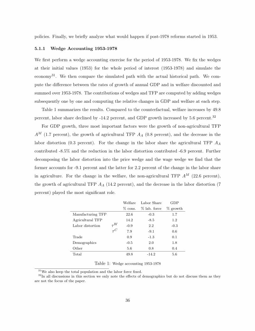
policies. Finally, we briefly analyze what would happen if post-1978 reforms started in 1953.

5.1.1 Wedge Accounting 1953-1978

We first perform a wedge accounting exercise for the period of 1953-1978. We fix the wedges

at their initial values (1953) for the whole period of interest (1953-1978) and simulate the

economy31. We then compare the simulated path with the actual historical path. We com-

pute the difference between the rates of growth of annual GDP and in welfare discounted and

summed over 1953-1978. The contributions of wedges and TFP are computed by adding wedges

subsequently one by one and computing the relative changes in GDP and welfare at each step.

Table 1 summarizes the results. Compared to the counterfactual, welfare increases by 49.8

percent, labor share declined by -14.2 percent, and GDP growth increased by 5.6 percent.32

For GDP growth, three most important factors were the growth of non-agricultural TFP

AM (1.7 percent), the growth of agricultural TFP AA (0.8 percent), and the decrease in the

labor distortion (0.3 percent). For the change in the labor share the agricultural TFP AA

contributed -8.5% and the reduction in the labor distortion contributed -6.9 percent. Further

decomposing the labor distortion into the price wedge and the wage wedge we find that the

former accounts for -9.1 percent and the latter for 2.2 percent of the change in the labor share

in agriculture. For the change in the welfare, the non-agricultural TFP AM (22.6 percent),

the growth of agricultural TFP AA (14.2 percent), and the decrease in the labor distortion (7

percent) played the most significant role.

Welfare Labor Share GDP% cons. % lab. force % growth

Manufacturing TFP 22.6 -0.3 1.7Agricultural TFP 14.2 -8.5 1.2Labor distortion τW -0.9 2.2 -0.3

τC 7.9 -9.1 0.6Trade 0.9 -1.3 0.1Demographics -0.5 2.0 1.8Other 5.6 0.8 0.4Total 49.8 -14.2 5.6

Table 1: Wedge accounting 1953-1978

31We also keep the total population and the labor force fixed.32In all discussions in this section we only note the effects of demographics but do not discuss them as they

are not the focus of the paper.

36

We now briefly compare the wedge accounting with the standard growth accounting in

Table 2

Capital Labor Aggregate TFP GDP

Non-agricultural TFP 0.8 0.0 0.9 1.7

Agricultural TFP 0.2 0.0 1.0 1.2

Labor distortion -0.5 0.0 0.8 0.3

Demographics 1.1 1.1 -0.4 1.8

Other Factors 0.8 0.0 -0.3 0.5

Total 2.4 1.1 2.0 5.6

Table 2: Decomposition of growth accounting: 1953-78

We note here that since the labor distortions exhibited a dramatic decline and then the

reversal during the GLF, their effects are muted in the analysis of the whole 1953-1978 period.

As we discuss in the next section, the behavior of the labor distortion plays a dominant role

during the GLF.

5.1.2 The Role of the Great Leap Forward

In this section, we simulate the behavior of the economy assuming that the Great Leap Forward

did not happen. Figure 5 plots the behavior of the actual and simulated wedges and sectoral

TFPs. We linearly extrapolate TFP in both sectors, the price wedge, the capital and labor

wedges between 1957 and 1964. We also linearly extrapolate the shares of export of agricultural

goods and imports of non-agricultural goods in respective value added between 1957 and 1970,

as the effect on trade was apparently somewhat more prolonged than on other wedges.

The key differences with the actual wedges are as follows. There is no drop in the man-

ufacturing TFP. There is no jump in 1958 and then no consequent fall in agricultural TFP.

There is no jump in the price wedge and the decrease in the labor distortion (normalized and

non-normalized). There is no sharp decline in defense spending. There is no expansion of

agricultural exports or the corresponding import of industrial equipment.

Figure 6 plots the behavior of actual and simulated real GDP, labor and value added

composition, sectoral consumption and capital stock. Fluctuations in most of the variables are

dampened in the absence of the GLF. In particular, the labor share remains stable around 85

percent, consumption of agricultural goods drop much less than it did during the famine, at

the expense of a somewhat lower path of non-agricultural consumption. The path of capital to

37

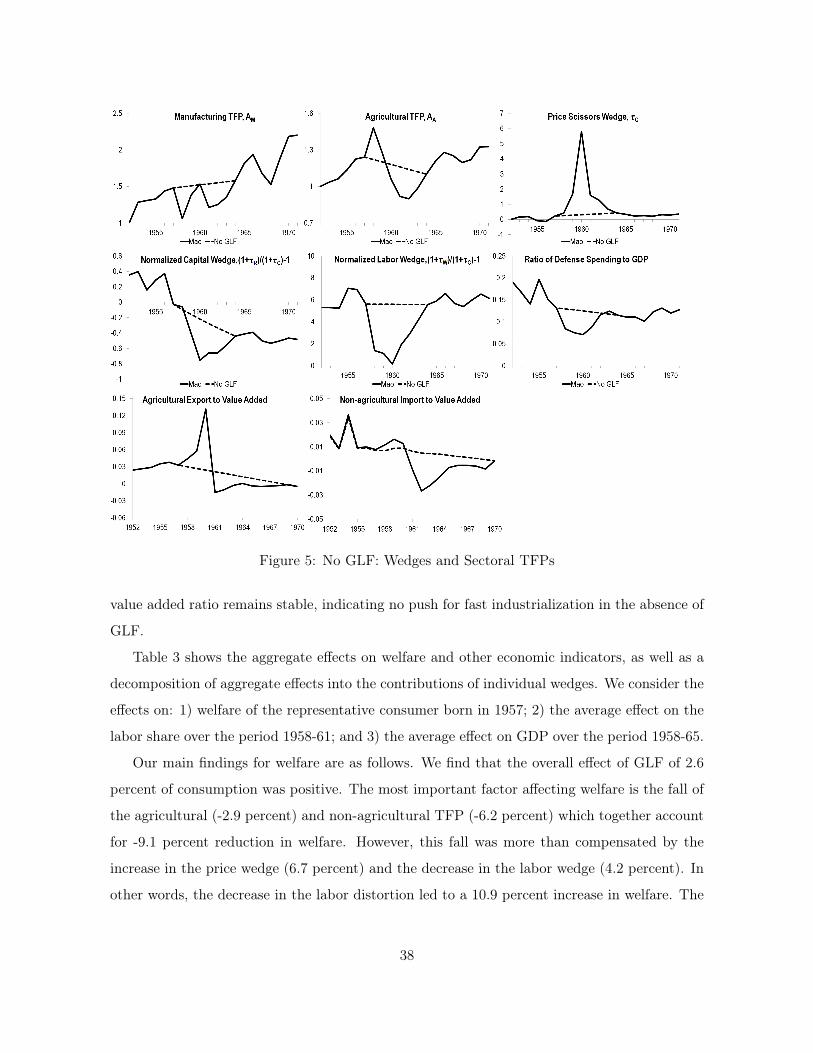
Figure 5: No GLF: Wedges and Sectoral TFPs

value added ratio remains stable, indicating no push for fast industrialization in the absence of

GLF.

Table 3 shows the aggregate effects on welfare and other economic indicators, as well as a

decomposition of aggregate effects into the contributions of individual wedges. We consider the

effects on: 1) welfare of the representative consumer born in 1957; 2) the average effect on the

labor share over the period 1958-61; and 3) the average effect on GDP over the period 1958-65.

Our main findings for welfare are as follows. We find that the overall effect of GLF of 2.6

percent of consumption was positive. The most important factor affecting welfare is the fall of

the agricultural (-2.9 percent) and non-agricultural TFP (-6.2 percent) which together account

for -9.1 percent reduction in welfare. However, this fall was more than compensated by the

increase in the price wedge (6.7 percent) and the decrease in the labor wedge (4.2 percent). In

other words, the decrease in the labor distortion led to a 10.9 percent increase in welfare. The

38

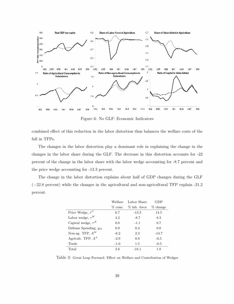
Figure 6: No GLF: Economic Indicators

combined effect of this reduction in the labor distortion thus balances the welfare costs of the

fall in TFPs.

The changes in the labor distortion play a dominant role in explaining the change in the

changes in the labor share during the GLF. The decrease in this distortion accounts for -22

percent of the change in the labor share with the labor wedge accounting for -8.7 percent and

the price wedge accounting for -13.3 percent.

The change in the labor distortion explains about half of GDP changes during the GLF

(+22.8 percent) while the changes in the agricultural and non-agricultural TFP explain -21.2

percent.

Welfare Labor Share GDP% cons. % lab. force % change

Price Wedge, τC 6.7 -13.3 14.5Labor wedge, τW 4.2 -8.7 8.3Capital wedge, τR 0.8 -1.1 0.7Defense Spending, gM 0.9 0.4 0.0Non-ag. TFP, AM -6.2 2.3 -14.7Agricult. TFP, AA -2.9 0.8 -6.5Trade -1.0 1.5 -0.5Total 2.6 -18.1 1.8

Table 3: Great Leap Forward: Effect on Welfare and Contribution of Wedges

39

It is also useful to look at the year-by-year decomposition of the effects on welfare of different

wedges which we present in Table 4. Interestingly, the only year in which the welfare effect of

the GLF was negative was 1960 (-3.9 percent of consumption).

1958 1959 1960 1961 1962 1963 1964 1965Price Wedge, τC 3.8 1.7 -2.7 8.4 9.5 12.0 12.8 11.7Labor wedge, τW 0.5 4.8 4.7 4.9 5.3 4.9 5.1 4.7Capital wedge, τR 0.3 1.5 2.1 0.7 0.2 0.1 0.4 0.4Defense Spending, gM 1.2 1.2 0.9 1.0 0.8 0.8 0.8 0.7Non-ag. TFP, AM -3.8 -6.2 -4.9 -5.0 -6.3 -7.9 -9.1 -8.4Agricult. TFP, AA 3.3 1.1 -2.4 -6.1 -7.4 -6.2 -3.8 -3.5Trade -0.6 -1.0 -1.7 -0.9 -0.8 -0.8 -0.8 -0.7Total 4.6 3.0 -3.9 2.9 1.4 1.4 5.5 4.9

Table 4: Great Leap Forward: Effect on Welfare and Contribution of Wedges by Year

Overall, the GLF was a very short episode of the disruption of the economy with the negative

welfare impact only in 1960. We note the importance of the changes in the labor distortion for

the behavior of the labor share and the GDP during that period.

5.1.3 Comparison with Collectivization in the USSR

The conclusion of the previous section that Great Leap Forward significantly reduced the labor

distortion while resulting in a significant fall in TFP naturally leads to the comparison with

the policies of the Soviet Union under Stalin.

We perform two counterfactual simulations. First, we start Stalin’s policies in 1957 (1956

thus being 1928 of Stalin’s policies). This choice of timing is guided by the idea that the peak

of the reforms in China under the Great Leap Forward (1960) should coincide with the peak of

Soviet collectivization (1932). This is done to isolate GLF, and to highlight striking similarities

as well as differences between the GLF and the most intense phase of Stalin’s collectivization.

This comparison highlights Mao’s way of transforming agriculture that was even more radical

than Stalin’s (see discussion in Section 4.3).33 Second, we impose Stalin’s policies starting in

1953. This is done, to compare the much milder initial collectivization period of the First-Five

Year Plan together with the Great Leap Forward to the much more brutal Soviet collectivization

and industrialization.33For a short survey of the existing literature on exactly this comparison see Yang (2008).

40

Comparing the effects of the GLF with Stalin’s Collectivization. Since Stalin’s

wedges and some policies during collectivization (Cheremukhin, et. al. 2013) are similar to

wedges in China during the Great Leap Forward, we choose the timing Stalin’s policies to co-

incide with those of the GLF. We impose the wedges and sectoral TFPs for Stalin’s 1928-1939

economy on our model of the Chinese economy over the period 1956-1967. We do this by multi-

plying each wedge by period-over-period relative changes in wedges implemented by Stalin. We

then compare the actual data for the Chinese economy to the simulated Chinese economy with

Stalin’s policies imposed. That is, the model in 1956-1967 has the same innovations to wedges

and sectoral TFP as that of Stalin. After 1967, the economy returns to the same growth rates

of wedges and the sectoral TFPs as in the baseline model.

Figure 7 plots both actual Chinese wedges and the simulated economy with Stalin’s wedges.

There are remarkable similarities between these economies and some important differences.

First, both the price wedges, the labor and capital wedges are virtually identical. The simi-

larities are consistent with our discussion in Section 4.3 and with Cheremukhin, et. al. (2013)

that the primary goals of both Chinese and Soviet economic policies were to move people from

agriculture to industry. Second, the policies both in China and Soviet Russia led to a collapse

of TFP. The fall of agricultural TFP from the peak to trough was 19 percent in Soviet Rus-

sia versus 40 percent in China. This is consistent with the more radical way of transforming

agriculture in China during the Great Leap Forward that we discussed in Section 4.3. The fall

of non-agricultural TFP from the peak to trough was 36 percent in Soviet Russia versus 28

percent in China. Third, and most importantly, the Great Leap Forward was much shorter

lasting than Stalin’s policies.

We summarize the behavior of the wedges and sectoral TFPs as follows. The size of the

changes in the wedges at the peak of the reforms were similar in China and USSR. The labor

distortion in China returned to the original high level promptly but was permanently reduced

in USSR. China had a more severe and slightly more protracted collapse of agricultural TFP

than USSR. The collapse of non-agricultural TFP was larger in China but was quickly reversed;

while in the USSR, the TFP in non-agriculture took much longer to recover.

Figure 8 plots the key variables for the simulated and actual economy. The most important

issues to notice are that the simulated Chinese economy with Stalin’s policies would have

achieved a much larger structural transformation with a significantly higher share of labor

41

Figure 7: Soviet Collectivization vs GLF: Wedges

force in non-agriculture (40 percent) compared to (20 percent) in the actual economy. As

noted earlier, the size of the changes in wedges in China during the GLF is essentially identical

to that under Stalin in Soviet Union’s First Five-Year Plan, but the changes to the labor

distortion were largely reversed in China, and not reversed in Soviet Russia. Similarly, the

differences in TFP (higher in agriculture, lower in manufacturing) persist in the USSR, but not

in China. However, these large shifts of factors of production have a very limited effect on the

paths of production and consumption, as they follow similar paths in China and USSR.

Table 5 shows the aggregate effects on welfare, and the labor share and GDP change as well

as contributions of individual wedges. Our main findings for welfare are as follows. We find the

overall effect of 3.9 percent of consumption. The most important factor affecting the difference

in welfare is that the fall in non-agricultural TFP was less severe in the Soviet economy. This

yields 25.8 percent of welfare. During the Great Leap Forward, the fall in the agricultural

TFP was larger, however, accounting for -3.7 percent of welfare. Stalin’s policies were more

successful in breaking the labor distortion. The of the reduction in the labor distortion was

-17.8 percent. The smaller decrease in the labor distortion under GLF policies accounted for

-16.7 percent. The effects of the price wedge were roughly comparable. The consequence of

this change is a 20.8 percent higher labor share in agriculture after the Great Leap Forward,

accounted almost fully by the combined effect of the higher labor distortion (21.1 percent).

42

Figure 8: Soviet Collectivization vs GLF: Economic Indicators

Welfare Labor Share GDP% cons. % lab. force % change

Price Wedge, τC -1.1 -1.0 -1.7Labor Wedge, τW -16.7 21.1 -13.1Capital wedge, τR -0.5 -0.2 -0.2Non-ag. TFP, AM 25.8 -2.1 22.4Agricult. TFP, AA -3.7 2.9 -8.5Total 3.9 20.8 -1.1

Table 5: Soviet Collectivization vs GLF: Welfare and Contribution of Wedges

The GDP changes also reflect the dominant role played by the behavior of TFP and the labor

distortion.

We summarize the results as follows. If China followed Soviet industrialization and col-

lectivization policies the results in terms of welfare would have been worse (and GDP slightly

lower) than a combination of the Great Leap Forward and the post-1962 retrenchment.The

Great Leap Forward and Stalin’s collectivization had similar effects on welfare at the peak

of the campaigns. The quick reversal of the policies under the Great Leap Forward led to a

significantly higher labor distortion in China but coincided with the recovery of the losses in

agricultural TFP. In contrast, Soviet collectivization would have achieved a long-term reduction

in the labor distortion at a cost of a long-term reduction in manufacturing TFP.

43

Comparing the effects of the FFYP and GLF with Stalin’s Collectivization. We now

turn to a slightly different view of China’s development strategy — comparing the combined

effects of the FFYP and the GLF starting in 1953 to Stalin’s collectivization.

The first First Five-Year Plan was modeled on that of the Soviet Union but still remained

rather distinct (see, e.g., “Part 1: Emulating Soviet Model” in MacFarquhar and Fairbank 1987

and Chapter 2 “Development Strategies and Policies in Contemporary China” in Eckstein 1977).

We briefly expand our discussion in Section 4.2 to focus on the differences between the policies

in China and USSR from 1953. The process of collectivization during the First Five-Year Plan

was a “gradual, stage-by-stage process, rather than the sudden and chaotic pattern of the Soviet

Union”. CCP avoided during the FFYP, the “single minded focus on extracting agricultural

surplus” (Teiwes 1987, p.141). Nolan (1976) in an insightful study compares the main features of

collectivization in China and the Soviet Union and argues for three key differences: (1) the core

explanation was the rural origin of the CCP reflecting the different way in which the revolution

happened; (2) the Chinese village was less polarized than in the Soviet Union limiting the

scope of expropriation; (3) the low level of agricultural output per capita forced China to the

more positive approach of trying to raise production and incomes as well as surplus extraction.

Nolan (1976, p. 194-195) concludes that “the process of collectivization was carried through

in fundamentally different ways in China and the Soviet Union, and with sharply contrasting

results. The disastrous losses sustained to the means of production in agriculture in Russia

during collectivization had a direct and lasting negative impact on agricultural output; the

losses sustained by China were of an altogether smaller magnitude.”34

Specifically, we start with initial values of agricultural and non-agricultural TFP and three

intersectoral wedges in 1952. We impose the wedges and sectoral TFPs calculated in Chere-

mukhin, et. al (2013) for Stalin’s 1928-1939 economy on our model of the Chinese economy.

We do this by multiplying each wedge by period-over-period relative changes in wedges imple-

mented by Stalin. We then compare the actual data for the Chinese economy to the simulated

Chinese economy with Stalin’s policies imposed. That is, the model in 1953-1964 has the same34To provide one example, Nolan (1976, Table 3 and 4) gives a number of comparative estimates on the

losses in live animals and grain output. Forced collectivization in Russia lead to the widespread slaughter ofthe draft animals that severely affected the amount of horsepower available in agriculture. The total amountof horsepower available was not recovered until late 1930s, even counting the tractors. In contrast, in China in1955-56 during the height of the campaign of collectivization there was only a small reduction in the stock ofdraft animals (Lardy 1987b, p. 157; Cheremukhin et. al 2013).

44

Welfare Labor Share GDP% cons. % lab. force % change

Price Wedge, τC -3.4 -1.1 -4.8Labor Wedge, τL -26.2 25.7 -13.6Capital Wedge, τR 1.5 -0.3 1.2Non-ag. TFP, AM 48.5 -2.3 24.4Agricult. TFP, AA 3.8 1.7 3.1Total 24.3 23.6 10.4

Table 6: Soviet Collectivization vs FFYP and GLF: Welfare and Contribution of Wedges

innovations to wedges and sectoral TFP as that of USSR. After 1964, the economy returns to

the same growth rates of wedges and sectoral TFPs as in the baseline model.

Figure 9 plots both actual Chinese wedges and the simulated economy with Stalin’s wedges.

Figure 10 plots the key variables for the simulated and actual economy. Table 6 shows the

aggregate effects on the economic indicators and welfare as well as contributions of individual

wedges. Our main finding is that Chinese policies in 1953-1964 lead to significantly higher

welfare (24.3 percent) compared to Stalin policies in 1928-1939. The difference in the effects of

the GLF versus collectivization are very similar to Section 5.1.3. However, China’s First Five-

Year Plan was indeed a very important success, especially, in the difference in non-agricultural

TFP (and also, albeit smaller, difference in agricultural TFP).

Figure 9: Soviet Collectivization vs FFYP and GLF: Wedges

45

Figure 10: Soviet Collectivization vs FFYP and GLF: Economic Indicators

5.1.4 Market Reforms Starting in 1953

We briefly note another, however, rather obvious counterfactual: what if post-1978 reforms

started in 1953. Specifically, we compare the actual data for the Chinese economy to the sim-

ulated Chinese economy with post-1978 policies. We impose trend changes in intersectoral

wedges and sectoral TFPs of 1978-2012 on the period of 1953-1978. For 1978-2011 we keep the

same changes to wedges and sectoral TFPs as calculated in Section 5. We find dramatically

higher welfare and GDP in the simulated economy, and equally dramatic structural transforma-

tion in terms of the labor share. In other words, if China started reforms earlier, its generation

1953 would have 28.6 percent higher welfare, 3.2 times higher GDP, and -31.9 percent labor

share by year 1978. By far the most important factor affecting the difference in welfare is the

difference in TFP.

5.2 Post-1978 Reforms

We conduct two experiments in this section. We first perform a wedge-accounting exercise for

the period of 1978-2011. Second, we simulate the continuation in the trends of the 1953-1978

policies in the post-1978 period to provide a benchmark against which to measure the success

of the post-1978 reforms.

46

5.2.1 Wedge Accounting 1978-2011

We first perform a wedge-accounting exercise for the period of 1978-2011. We fix wedges at their

initial values (1978) for the whole period of interest (1978-2011) and simulate the economy35.

We then compare the simulated path with the actual historical path.

Table 7 summarizes the results. Compared to the counterfactual, welfare increases by 99.1

percent, labor share declines by -28.8 percent, and GDP growth increases by 9.4 percent. For

GDP growth, three most important factors were the growth of non-agricultural TFP AM (5.5

percent), the decrease in the labor distortion (1 percent), and the growth of agricultural TFP

AA (0.8 percent). For the change in the labor share, the reduction in the labor distortion

contributed -19 percent and the agricultural TFP AA contributed -12.7 percent. Further de-

composing the labor distortion into the price wedge and the wage wedge we find that the former

accounts for -14.9 percent and the latter for -4.1 percent of the change in the labor share in

agriculture. For the change in the welfare, the non-agricultural TFP AM (49.8 percent), the

growth of agricultural TFP AA (19.9 percent), and the decrease in the labor distortion (16.2

percent) played the most significant role.

Welfare Labor Share GDP% cons. % lab. force % growth

Manufacturing TFP 49.8 0.9 5.5Agricultural TFP 19.9 -12.7 0.8Labor Distortion τW 8.9 -4.1 0.3

τC 7.3 -14.9 0.7Trade -2.1 0.4 0.0Demographics 10.6 -2.6 1.8Other 4.8 4.2 0.2Total 99.1 -28.8 9.4

Table 7: Wedge Accounting 1978-2011

We also compare the wedge-accounting with the standard growth accounting for this period

in Table 8.35As in the wedge accounting simulation for the pre-reform period, here we also assume that the in the

simulated economy the intertemporal wedge is equal to zero.

47

Capital Labor Aggregate TFP GDP

Non-agricultural TFP 2.3 0.0 3.2 5.5

Agricultural TFP 0.7 0.0 0.1 0.8

Labor Distortion 0.7 0.0 0.3 1.0

Demographics 1.1 0.7 0.0 1.8

Other Factors 0.5 0.0 -0.3 0.2

Total 5.3 0.7 3.3 9.4

Table 8: Decomposition of growth accounting: 1978-11

We finish this section with Figure 11 and Figure 12 that highlight the importance of the

contributions of the changes in the labor distortions in both the changes in the labor share and

the GDP growth in the 1953-2011. The same breakdown is documented in Tables 9 and 10.

53-57 57-60 60-68 68-77 77-84 84-98 98-11Non-agricultural TFP, AM 1.5 1.3 -0.9 4.1 0.1 5.8 7.1Agricultural TFP, AA 4.2 -3.5 0.5 2.0 3.2 0.6 0.2Labor Distortion, τW ,τC -1.6 9.5 -3.1 0.6 1.4 1.2 0.7Demographics 1.5 3.2 2.1 1.2 2.5 2.0 1.1Other factors 1.9 -1.3 2.0 -0.3 1.2 0.0 0.5Total 7.4 9.1 0.6 7.5 9.2 9.6 9.5

Table 9: Wedge accounting for GDP per capita: 1953-2011

53-57 57-60 60-68 68-77 77-84 84-98 98-11Non-agricultural TFP, AM 1.5 1.3 -0.9 -4.2 6.7 -3.1 -2.7Agricultural TFP, AA -3.8 2.9 0.0 -5.8 -6.3 -3.5 -2.9Labor Distortion, τW ,τC 4.5 -24.9 24.0 -7.2 -3.2 -7.6 -5.5Demographics 0.0 -2.0 0.4 3.1 -1.5 0.0 -1.0Other factors -5.3 5.0 -2.6 -0.2 0.4 2.9 -1.4Total -3.2 -17.8 20.9 -14.2 -3.9 -11.4 -13.6

Table 10: Wedge accounting for labor share: 1953-2011

48

Figure 11: Contributions to Labor Reallocation by period: 1953-2011.

Figure 12: Contributions to Growth by period: 1953-2011.

5.2.2 China Without Post-1978 Reforms

In this section, we consider a key benchmark against which to measure the success of the

post-1978 reforms: what if 1953-1978 policies continued after 1978.

Specifically, we compare the actual data for the Chinese economy to the simulated Chinese

economy with 1953-1978 policies continued. We preserve the wedges for the period 1952-1973,

and impose the average trends in wedges and sectoral TFPs of 1953-1978 (excluding GLF)

49

on the period 1974-2011 (there is a brief 1974-77 transition period towards trend to eliminate

large jumps towards the trend line). Figure 13 plots both actual Chinese wedges and the

simulated economy with 1953-1978 policies extended after 1978; Figure 14 plots the main

economic indicators.

Figure 13: No Market Reforms in 1978: Wedges and Sectoral TFPs

Table 11 shows the aggregate effects on the economic indicators (their average level in year

2000) and welfare of generation 1978, as well as contributions of individual wedges. Specifically,

this table shows the difference of the actual over the simulated economy.

We find that the welfare is higher by 46.4 percent with the decreased labor distortion playing

the most important role (19.8 percent) and the higher growth of the agricultural (10.5 percent)

and non-agricultural (9.6) TFP being two other important factors.

The decreased labor distortion plays a dominant role in explaining the change in the labor

share (-17.8 percent) and is followed in importance by the higher growth of agricultural TFP

(-7.8 percent).

50

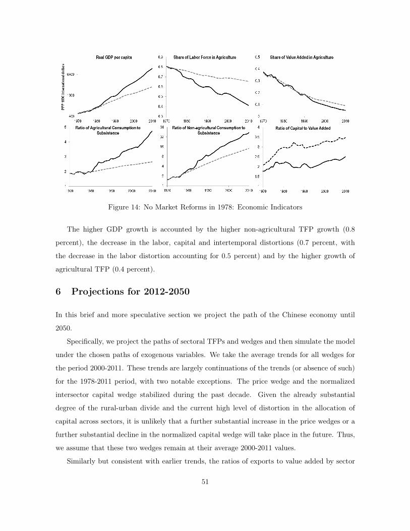
Figure 14: No Market Reforms in 1978: Economic Indicators

The higher GDP growth is accounted by the higher non-agricultural TFP growth (0.8

percent), the decrease in the labor, capital and intertemporal distortions (0.7 percent, with

the decrease in the labor distortion accounting for 0.5 percent) and by the higher growth of

agricultural TFP (0.4 percent).

6 Projections for 2012-2050

In this brief and more speculative section we project the path of the Chinese economy until

2050.

Specifically, we project the paths of sectoral TFPs and wedges and then simulate the model

under the chosen paths of exogenous variables. We take the average trends for all wedges for

the period 2000-2011. These trends are largely continuations of the trends (or absence of such)

for the 1978-2011 period, with two notable exceptions. The price wedge and the normalized

intersector capital wedge stabilized during the past decade. Given the already substantial

degree of the rural-urban divide and the current high level of distortion in the allocation of

capital across sectors, it is unlikely that a further substantial increase in the price wedges or a

further substantial decline in the normalized capital wedge will take place in the future. Thus,

we assume that these two wedges remain at their average 2000-2011 values.

Similarly but consistent with earlier trends, the ratios of exports to value added by sector

51

Actual No Reforms Welfare Labor Share ∆GDP% gr. rate % gr. rate % cons. % lab. force % growth

Labor Distortion τW and τC -2.3 -1.0 19.8 -17.8 0.5τW -0.1 0.7 3.8 -11.0 0.3τC 2.2 1.7 16.0 -6.8 0.2

Capital Distortion τR and τC -1.8 -5.4 0.8 -2.3 0.1Government gM 4.7 2.5 0.0Non-ag. TFP, AM 4.5 2.4 9.6 1.4 0.8Agricult. TFP AA 3.1 1.3 10.5 -7.8 0.4Capital wedge τK 2.7 -2.6 0.1Trade -1.6 -0.8 0.1Total 46.4 -27.3 2.0

Table 11: No Market Reforms in 1978: Welfare and Contribution of Wedges

and the ratio of defense spending to GDP are assumed to stay constant at their average 2000-

2011 levels. Population and labor force are assumed to continue growing at the same rates as

in 2000-2011. The normalized intersector labor wedge is assumed to keep declining at the same

rate as in the 2000-2011 period. The intertemporal capital wedge is assumed to converge to its

average 2000-2011 level from its 2011 level.

We assume that both agricultural and non-agricultural TFP continue growing initially at

their average 2000-2011 growth rates. However, at their current speed, TFP in both sectors

is bound to exceed by orders of magnitude the level of TFP in the USA by 2050. We thus

assume that, after Chinese TFP in either sector reaches the level of 70 percent of the US TFP,

it slows down its growth and exponentially converges to US trend, as shown in Figure 15. These

assumptions imply that non-agricultural TFP growth will slow down within the next 10 years,

while agricultural TFP will keep growing at current rates until around 2030. These projections

are consistent with the large literature on growth convergence, which documents that the closer

a country is to the frontier, the slower its growth rate.

52

Figure 15: Actual and projected wedges in China in 2000-2050.

Figure 16 further describes the simulated path of the Chinese economy. Our projection

implies a stable share of investment in GDP at 40 percent. The movement of labor from

agriculture to other sectors will continue, with the labor share in agriculture declining from 40

percent in 2010 to 25 percent in 2050. The share of value added by the agricultural sector will

reach 2 percent in 2050 from 5 percent currently. The level of GDP per capita will approach

that of the US by 2040, when China will likely be considered a developed country.

Figure 16: Actual and projected economic indicators in China in 2000-2050.

53

Finally, we summarize the results of the comparison of the wedge and growth accounting

for the simulated 2011-2050 economy in Table 12 and for the wedge accounting by different

periods in Table 13.

Capital Labor Aggregate TFP GDPDemographics, N , POP 0.0 0.5 0.0 0.5Labor Distortion 0.3 0.0 0.5 0.8Non-agricultural TFP, AM 1.5 0.0 2.5 4.0Agricultural TFP, AA 0.0 0.0 0.2 0.2Total 1.8 0.5 3.2 5.5

Table 12: Decomposition of growth accounting: 2011-50

11-20 20-30 30-50 2011-50Labor Distortion, τL 0.7 0.7 0.8 0.8Non-agricultural TFP, AM 7.0 4.5 2.5 4.0Agricultural TFP, AA 0.4 0.4 0.0 0.2Total 8.1 5.6 3.3 5.0

Table 13: Wedge accounting for projected GDP per capita: 2011-2050

7 Conclusions

This paper provides a unified treatment of the 1953-2011 period of economic development of

People’s Republic of China. First, we find the importance of the change in the labor distortions

in the structural transformation. These changes are at least as important as the changes

in agricultural TFP emphasized by models of structural transformation. Moreover, further

decomposing the labor distortion we find that the changes in the price wedge rather than the

wage wedge play key role. Second, we provide a careful analysis of the important changes in

the economy of China in 1953-1978 and assess the key driving factors behind these changes.

As such, the model is a useful lens through which to view different policies implemented during

that time of a significant transformation of the country. Third, our analysis of 1953-1978 serves

as a key benchmark against which to compare the success of reforms in post-1978 period. We

find that continuation of 1953-1978 policies would lead to a 2 percent per year slower growth

and a significantly smaller share of of the non-agriculture. Again, one of the key determinants

of these differences are the changes in the labor distortions. Overall, our conclusion is that the

study of 1953-1978 reforms is not only interesting because of the policies implemented during

54

that time, but also as an essential initial point for the analysis of the post-1978 Chinese growth.

55

8 References

Acemoglu, Daron and Veronica Guerrieri, “Capital Deepening and Non–Balanced Economic

Growth,” Journal of Political Economy, 2008, 116, 467–498.

Borensztein, Eduardo, and Jonathan D. Ostry (1996) “Accounting for China’s Growth Per-

formance” The American Economic Review, Papers and Proceedings, 86(2), pp 224-228.

Brandt, Loren (1997). “Reflections on China’s Late 19th and Early 20th-century Economy.”

The China Quarterly, 150, pp. 282-308.

Brandt, Loren, Hsieh, Chang-Tai, and Xiadong Zhu (2008) “Growth, and Structural Trans-

formation in China,” in Loren Brandt and Thomas Rawski ed., China’s Great Economic Trans-

formation. Cambridge University Press.

Brandt, Loren, and Xiaodong Zhu (2010) “Accounting for China’s growth,” IZA Discussion

Paper No. 4764.

Brandt, Loren, Trevor Tombe, and Xiadong Zhu (2013) “Factor Market Distortions across

Time, Space, and Sectors in China,” Review of Economic Dynamics, 16(1), pp. 39-58.

Buera, Francisco J., and Joe P. Kaboski (2009). “Can traditional theories of structural

change fit the data?” Journal of the European Economic Association, 7 (2-3), pp. 469-477.

Buera, Francisco J., and Joe P. Kaboski (2012) “Scale and the origins of structural change”,

Journal of Economic Theory, 147(2), pp. 684-712.

Cai, Fang, Albert Park, and Yaohui Zhao (2008). “The Chinese Labor Market in the Re-

form Era,” in Loren Brandt and Thomas Rawski ed., China’s Great Economic Transformation.

Cambridge University Press.

Cao, Yuanzheng, Yingyi Qian, and Barry R. Weingast (1999) “From Federalism, Chinese

Style, to Privatization, Chinese Style,” Economics of Transition, 7(1), 103-131.

Caselli, Francesco, and Wilbur John II. Coleman (2001) “The U.S. structural transformation

and regional convergence: A reinterpretation,” Journal of Political Economy, 109(3), pp. 584-

616.

Chai, Joseph, C.H. (1992) “Consumption and living standard in China”, The China Quar-

terly, 131, pp. 721-49.

Chan, Kam Wing and Li Zhang, (1999). “The Hukou System and Rural-urban Migration:

Processes and Changes,” The China Quarterly, 160(1), pp. 818-855.

56

Chari, V. V., Patrick Kehoe, and Ellen McGrattan (2007) “Business cycle accounting,”

Econometrica, 75(3), pp. 781-836.

Chen, Derong (1995) “Chinese Firms Between Hierarchy and Market: The Contract Man-

agement Responsibility System” London: Macmillan.

Cheng, Tiejun and Mark Selden (1994) “The Origins and Social Consequences of China’s

Hukou System”, The China Quarterly, 139, pp. 644-668.

Cheremukhin, Anton, Mikhail, Golosov, Sergei Guriev, and Aleh Tsyvinski (2013) “Was

Stalin Necessary for Russia’s Economic Development?” NBER Working Paper No. 19425.

Choe, Chongwoo and Xiangkang Yin (2000) “Contract management responsibility system

and profit incentives in China’s state-owned enterprises,” China Economic Review, 11(1), pp.

98-112.

Chow, Gregory (1985) “A Model of Chinese National Income Determination,” Journal of

Political Economy, 93(4), pp. 782-792.

Chow, Gregory (1993) “Capital Formation and Economic Growth in China,” Quarterly

Journal of Economics, 108(3), pp. 809-842.

Chow, Gregory, and Kui-Wai Li (2002) “China’s Economic Growth: 1952–2010,” Economic

Development and Cultural Change, 51(1), pp. 247-256.

Cole, Harold L., and Lee E. Ohanian (2004) “New deal policies and the persistence of the

great depression: A general equilibrium analysis,” Journal of Political Economy, 112(4), pp.

779-816.

Dekle, Robert, and Guillaume Vandenbroucke (2012) “A quantitative analysis of China’s

structural transformation,” Journal of Economic Dynamics and Control 36, 119–135.

Eckstein, Alexander (1975) China’s Economic Development. University of Michigan Press.

Eckstein, Alexander (1977) China’s Economic Revolution. Cambridge University Press.

Estrin, Saul, Jan Hanousek, Evzen Kocenda, and Jan Svejnar (2009) “The Effects of Pri-

vatization and Ownership in Transition Economies,” Journal of Economic Literature 47(3),

699–728.

Fernald, John and Brent Neiman (2011), "Growth Accounting with Misallocation: Or,

Doing Less with More in Singapore", American Economic Journal: Macroeconomics, 3(2),

p.29-74.

Fukao, Kyoji, Kozo Kiyota, and Ximing Yue (2006) “China’s Long-Term International Trade

57

Statistics: By Commodity, 1952-1964 and 1981-2000,” Hi-Stat Discussion Paper Series d05-147,

Institute of Economic Research, Hitotsubashi University.

Feurwerker, Albert (1977) “Economic Trends in the Republic of China 1912-49.” Ann Arbor.

University of Michigan, Michigan Papers in Chinese Studies no. 31. Cited in Richardson (1999,

p. 47).

Gan, Jie, Yan Guo, and Chenggang Xu (2010) “Privatization and the Change of Control

Rights: The Case of China,” mimeo, London School of Economics.

Groves, Theodore, Yongmiao, Hong, John McMillan, and Barry Naughton (1994) ‘‘Auton-

omy and Incentives in Chinese State Enterprises,’’ Quarterly Journal of Economics, 109(1), pp

183–209.

Guriev, Sergei, and William L. Megginson (2007) “Privatization: What Have We Learned?”

In Beyond Transition, ed. Francois Bourguignon and Boris Pleskovic, 249–96. Washington,

D.C.: World Bank.

Hayashi, Fumio, and Edward C. Prescott (2008) “The depressing effect of agricultural insti-

tutions on the prewar Japanese economy,” Journal of Political Economy, 116(4), pp. 573-632.

Herrendorf, B., Rogerson, R., andValentinyi, A. (2013). “Growth and Structural Transfor-

mation (No. w18996). National Bureau of Economic Research.

Holz, Carsten (2006) “Measuring Chinese Productivity Growth, 1952-2005,” manuscript,

Hong Kong University of Science and Technology.

Hsiao, Liang-Lin (1974) “China’s Foreign Trade Statistics’ 1864-1949.” Cited in Richardson

(1999, p. 46).

Hsieh, Chang-Tai, and Peter Klenow (2009) “Misallocation and Manufacturing TFP in

China and India,” Quaterly Journal of Economics 124(4), pp. 1403-48.

Hsueh, Tien-tung, and Qiang Li (1999) “China’s national income, 1952-1995” Westview

Press.

Huang, Jikun, Keijiro Otsuka, and Scott Rozelle (2008) “Agriculture in China’s Develop-

ment: Past Disappointments, Recent Successes, and Future Challenges,” in Loren Brandt and

Thomas Rawski, ed., “China’s Great Economic Transformation,” Cambridge University Press.

Huang, Jikun, and Scott Rozelle (1996) “Technological Change: Rediscovering the Engine

of Productivity Growth in China’s Agricultural Economy,” Journal of Development Economics,

49(2), pp. 337–369.

58

Jefferson, Gary H. and Thomas G. Rawski (1994) “Enterprise Reform in Chinese Industry,”

Journal of Economic Perspectives, 8(2), pp. 47-70.

Kueh, Yak-Yeow(1995) “Agricultural instability in China, 1931–1991” Clarendon Press: Ox-

ford.

Kongsamut, Piyabha, Sergio Rebelo, and Danyang Xie, “Beyond Balanced Growth,” Review

of Economic Studies, 2001, 68, 869–882.

Lardy, Nicholas (1987a) “Economic Recovery and the First Five-Year Plan”, Chapter 3 in

MacFarquhar, Roderick and John K. Fairbank, ed., The Cambridge History of China, Vol-

ume 14, The People’s Republic, Part I: The Emergence of Revolutionary China 1949-1965.

Cambridge University Press.

Lardy, Nicholas (1987b), “The Chinese Economy under Stress, 1958-1965”, Chapter 8 in

MacFarquhar, Roderick and John K. Fairbank, ed., The Cambridge History of China, Vol-

ume 14, The People’s Republic, Part I: The Emergence of Revolutionary China 1949-1965.

Cambridge University Press.

Lardy, Nicholas (1994)“Consumption and living standards in China, 1978-83,” The China

Quarterly, 100, pp. 849-65.

Lau, Lawrence, Yingyi Qian, and Gerard Roland (2000) “Reform without Losers: An Inter-

pretation of China’s Dual-Track Approach to Transition,” Journal of Political Economy, 108(1),

pp. 120–43.

Li, David D. (1998) “Changing Incentives of the Chinese Bureaucracy,” American Economic

Review, Papers and Proceedings, 88(2), pp. 393-397.

Li, Guo, Scott Rozelle, and Loren Brandt (1998) “Tenure, land rights, and farmer investment

incentives in China,” Agricultural Economics 19 (1-2), pp. 63-71.

Li, Hongbin, Lei Li, Binzhen Wu, and Yanyan Xiong (2012) “The End of Cheap Chinese

Labor,” Journal of Economic Perspectives, 26 (4), pp 57-74.

Li, Wei (1997) “The Impact of Economic Reform on the Performance of Chinese State

Enterprises, 1980–1989,” Journal of Political Economy, 105(5), pp. 1080-1106.

Li, Wei, and Dennis Tao Yang (2005) “The Great Leap Forward: Anatomy of a Central

Planning Disaster,” Journal of Political Economy 113(4), pp. 840-870.

Lin, Justin Yifu (1988) “The Household Responsibility System in China’s Agricultural Re-

form: A Theoretical and Empirical Study,” Economic Development and Cultural Change, 36

59

(supplement), 199-224.

Lin, Justin Yifu (1990), “Collectivization and China’s Agricultural Crisis in 1959-1961,”

Journal of Political Economy, 98(6), pp. 1228-1252.

Lin, Justin Yifu (1992) “Rural reforms and agricultural growth in China,” The American

Economic Review, 82(1), pp 34-51.

Lin, Justin Yifu (2012) “Demystifying the Chinese Economy” Cambridge University Press.

Lin, Justin Yifu and Miaojie Yu (2008) "The Economics of Price Scissors: An Empirical

Investigation for China." China Center for Economic Research, NO. E 2008001.

MacFarquhar, Roderick (1991) “The succession to Mao and the end of Maoism,” Chapter

4 in The Cambridge History of China, Volume 15, The People’s Republic, Part 2: Revolutions

within the Chinese Revolution 1966-1982, Cambridge University Press.

MacFarquhar, Roderick, and John K. Fairbank (1987) “The Cambridge History of China,

Volume 14, The People’s Republic, Part I: The Emergence of Revolutionary China 1949-1965,”

Cambridge University Press.

Ngai, L. Rachel and Chrisopher A. Pissarides, “Structural Change in a Multisector Model

of Growth,” American Economic Review, 2007, 97, 429–443.

Xin Meng (2012) “Labor Market Outcomes and Reforms in China,” Journal of Economic

Perspectives, 26 (4), pp 75-102.

Meng, Xin, Nancy Qian, and Pierre Yared (2013) “The Institutional Causes of China’s Great

Famine, 1959-61,” Mimeo, Yale.

McMillan, John, John Whalley and Lijing Zhu (1989) “The Impact of China’s Economic

Reforms on Agricultural Productivity Growth,” Journal of Political Economy, 97(4), pp. 781-

807.

Naughton, Barry (1993) “Deng Xiaoping: The Economist,” The China Quarterly, 135,

Special Issue: “Deng Xiaoping: An Assessment”, pp. 491-514.

Naughton, Barry (2007) The Chinese Economy: Transformation and Growth. MIT Press.

Nolan, Peter (1976) “Collectivization in China: Some comparisons with the USSR,” The

Journal of Peasant Studies, 3(2), 192-220.

Nolan, Peter, and Gordon White (2008) “Urban bias, rural bias or state bias? Urban-rural

relations in post-revolutionary China,” Journal of Development Studies, 20(3), 52-81.

Perkins, Dwight (1973) “Plans and Their Implementation in the People’s Republic of

60

China,” American Economic Review Papers and Proceedings, 63(2), pp. 224-231.

Perkins, Dwight (1975) “Growth and structural change of China’s 20th century economy”

In Perkins, Dwight, ed. China’s modern economy in historical perspective. Stanford University

Press.

Perkins, Dwight (1991) “China’s Economic Policy and Performance” In MacFarquhar, Rod-

erick, and John K. Fairbank, ed., The Cambridge History of China, Vol. 15. Cambridge

University Press.

Rozman, Gilbert, ed. (1981) The Modernization of China. New York: The Free Press.

Riskin, C (1975) “Surplus and stagnation in modern China” in Perkins, Dwight, ed. China’s

Modern Economy in Historical Perspective. Stanford University Press.

Rawski, Thomas (1979) Economic Growth and Employment in China. Oxford University

Press.

Richardson, Philip (1999) Economic Change in China c.1800-1950. Cambridge University

Press.

Schram, Stuart (1991) “Mao Tse-tung’s thought from 1949 to 1976.” In MacFarquhar, Rod-

erick, and John K. Fairbank, ed., The Cambridge History of China, Vol. 15. Cambridge

University Press.

Mark Selden (1979)“The People’s Republic of China. A Documentary History of Revolu-

tionary China. New York: Monthly Review Press.

Song, Zheng, Kjetil Storesletten, and Fabrizio Zilibotti (2011) “Growing Like China,” Amer-

ican Economic Review, 101 (1), pp 196–233.

Spence, Jonathan (2013) “The Search for Modern China”, Third Edition, W.W. Norton &

Company.

Statistical Yearbook (2012). Zhongguo tongji nianjian (Statistical Yearbook of China).

Beijing: Zhongguo tongji chubanshe.

Stokey, Nancy (2001) “A quantitative model of the British industrial revolution, 1780-1850”.

Carnegie-Rochester Conference Series on Public Policy, 55(1), pp. 55-109.

Teiwes, Frederick (1987) “Establishment and consolidation of the new regime,” In Mac-

Farquhar, Roderick, and John K. Fairbank, ed., The Cambridge History of China, Vol. 14.

Cambridge University Press.

Ungor, Murat (2011) “Some Aspects of the Chinese Industrialization.” Mimeo, Central

61

Bank of the Republic of Turkey.

Wang, Yan and Yudong Yao (2003) “Sources of China’s economic growth 1952–1999: in-

corporating human capital accumulation,” China Economic Review, 14(1), pp. 32–52.

Wang, Feng, and Xuejin Zuo (1999) “Inside China’s Cities: Institutional Barriers and Op-

portunities for Urban Migrants” American Economic Review, 89(2), 276-280.

Wu, Jinglian, and Zhao, Renwei (1987) “The Dual Pricing System in China’s Industry”

Journal of Comparative Economics, 11(3), pp 309–18.

Xu, Chenggang (2011) “The Fundamental Institutions of China’s Reforms and Develop-

ment,” Journal of Economic Literature, 49(4), pp. 1076-1151.

Yang, Alwyn (2003) “Gold into Base Metals: Productivity Growth in the People’s Republic

of China during the Reform Period,” Journal of Political Economy, 111 (6), pp. 1220-1261.

Yang, Dennis Tao (1997) "China’s Land Arrangements and Rural Labor Mobility," China

Economic Review, 18(2), pp. 101-15.

Yang, Dennis Tao (1999) "Urban-biased policies and rising income inequality in China,"

American Economic Review 89(2), pp. 306-310.

Yang, Dennis Tao (2008) “China’s Agricultural Crisis and Famine of 1959–1961: A Survey

and Comparison to Soviet Famines,” Comparative Economic Studies, 50, pp 1–29.

Yang, Dennis Tao, and Hao Zhou (1999) "Rural-urban disparity and sectoral labour allo-

cation in China," Journal of Development Studies 35(3), pp. 105-133.

Yu, Miaojie, and Justin Y. Lin (2008) “The Economics of Price Scissors: An Empirical

Investigation for China,” available at SSRN: http://ssrn.com/abstract=1032404.

Zhu, Xiaodong (2012) “Understanding China’s Economic Growth: Past, Present and Fu-

ture,” Journal of Economic Perspectives, 26(4), pp. 103-24.

62