The Economics of Trade Disputes,

the GATT’s Article XXIII, and

the WTO’s Dispute Settlement Understanding

Chad P. Bown†,‡

Department of Economics andGraduate School of International Economics and Finance

Brandeis UniversityRevised Version: January 2002

Abstract

Economic theory has yet to provide a convincing argument that can explain whythe threat of retaliation under the GATT/WTO dispute settlement procedures is not suf-ficient to prevent countries from violating the agreement. We consider the question of whycountries violate the agreed-upon rules in the face of explicit provisions which allow themto legally adjust their trade policy. Using the GATT/WTO institutional structure and theguiding principle of reciprocity, we provide a theory suggesting when countries will chooseto implement protection in violation of GATT/WTO rules, as opposed to under the relevantsafeguards provisions, when trade policy adjustments are necessary between ‘negotiatingrounds.’

JEL No. F13Keywords: Trade Disputes; GATT; WTO; Reciprocity; Political Economy; Terms of Trade

† correspondence: Department of Economics, MS 021, Brandeis University, Waltham, MA02454-9110 USAtel: (781) 736-4823, fax: (781) 736-2269, email: cbown@brandeis.edu

‡ I gratefully acknowledge financial support from the Mellon Foundation through an Eco-nomics Department Granick Fellowship at the University of Wisconsin. I would like to thankRobert Staiger for his advice and Peter Rosendorff, Wolfgang Keller, Robert Baldwin, Gre-gory Shaffer, Alan Sykes, David Vanness, Mikhail Klimenko, two anonymous referees andseminar participants at the University of Wisconsin and the University of California-SantaCruz for helpful comments. All remaining errors are my own.

1 Introduction

Since 1947 over 140 countries have either signed the original General Agreement on Tariffs and Trade

(GATT 1947) or have become members of the World Trade Organization (WTO). Under these agree-

ments, countries subject themselves to rules that place limitations on their available trade policies,

bind tariffs to agreed-upon levels and prohibit most other non-tariff barriers to trade. Article XXIII

of the GATT 1947 and the Dispute Settlement Understanding (DSU) of the WTO provide fora to

which countries bring grievances claiming that other participating countries have violated the agreed-

upon rules-of-trade. Legal scholars such as Dam (1970) have emphasized that the GATT system is

structured so that countries that are injured by rules violations are authorized to threaten retaliation

under the dispute settlement mechanism so that the agreements may maintain a balance of obligations.

Yet even in the presence of such a system, trade disputes in which countries deliberately violate the

GATT/WTO rules are frequent to occur. Since its 1995 inception, the WTO has been notified of over

240 complaints (WTO, 2001). The central purpose of this paper is to provide an economic framework

that can be used to further our understanding of the dispute settlement mechanism and to interpret

the role of disputes in the formal institutions of international trade.

The normative role of the GATT/WTO dispute settlement mechanism has been a subject of con-

siderable historic controversy, and as Jackson states,

A number of interesting policy issues are raised by the experience of the [dispute settlement] procedure,

not the least of which is the question of what should be the fundamental objective of the system - to solve

the instant dispute (by conciliation, obfuscation, power threats or other means), or to promote certain

longer-term goals... The historical question is whether the GATT preparatory work and practice through

its decades establishes a goal of dispute-settlement more oriented toward “conciliation and negotiation” or

toward “rule integrity.” (Jackson, 1989, pp. 92-93)

In the economics literature, analysis of the dispute settlement mechanism has focused almost exclu-

sively on Jackson’s “rule integrity” orientation. Theorists typically model the mechanism as a trigger

strategy (i.e. a policy that governments will enact so as to follow a given ‘rule’) in an infinitely-repeated,

noncooperative, tariff-setting game between countries, exploring the mechanism’s role in supporting

low equilibrium tariffs (i.e. one important “longer-term goal” of the GATT).1 However, the typical

equilibria of these models either never exhibit trade disputes, or the equilibria exhibit disputes that are1Riezman (1991), Hungerford (1991) and Ludema (2001) use this structure in a bilateral setting, as does Maggi (1999)

in a multilateral setting. This line of analysis applies the dynamic oligopoly theory of implicit collusion of Green

and Porter (1984) and Rotemberg and Saloner (1986) to the implicit enforcement of trade policy in a dynamic tariff-

setting game between countries. Relying on the notion of “international obligation,” Kovenock and Thursby (1992)

add a cooperative component to this structure by allowing countries to violate the agreement at some positive cost.

Staiger (1995, pp. 1519-28) provides a more complete survey of this literature.

1

automatically triggered after the observance of a random fluctuation, such as a terms of trade change.2

Once the structure of the GATT institution is taken as given, the trade disputes are neither avoidable

nor the result of a deliberate, rational policy choice of a government.

Our first contribution is to focus on Jackson’s alternative “conciliation and negotiation” aspect

of the dispute settlement mechanism, which we feel has largely been ignored.3 However, in order to

provide a convincing interpretation of this role, we must determine why a country that seeks flexibility

in its trade policy chooses to deliberately disregard GATT rules and its obligations, even knowing

that it would be caught and that a trade dispute would result. There are, of course, explicit GATT

safeguards provisions whose purpose is to give governments flexibility under the agreement so that they

may ‘legally’ alter their trade policy and avoid disputes.4 To understand the GATT/WTO dispute

settlement mechanism and the basis of the disputes, we attempt to justify one motive for why countries

sometimes prefer to implement policies in violation of GATT/WTO rules or their obligations, so that

negotiations occur under the dispute settlement mechanism, as opposed to implementing the policies

in a manner that would allow for negotiations to be held under the GATT’s safeguards provisions.

In order to better motivate our perspective, consider the issues that most frequently lead to a trade

dispute. Most disputes under the GATT regime, for example, involved a claim that a government had

provided more protection for an import-competing industry than it had stipulated it would limit itself

to in a prior negotiating round. Table 1 illustrates this by providing a description of the trade disputes

that occurred during the GATT tenure. Of these 254 trade disputes, over 81% (206) involve such a

claim: a country has violated the GATT rules in order to provide excessive import protection. The most

common infractions were countries using quantitative restrictions to limit trade (violations of Article

XI), but countries have also failed to observe the rules on MFN (Article I), national treatment (Article

III), subsidies (Article XVI) or the various Codes of the Tokyo Round, or have failed to implement

lower negotiated tariffs thereby nullifying expected benefits (Article II). The other 48 cases primarily

involve the use of subsidy policies for export promotion (violating Article XVI), though there have

been instances in which disputes occurred over trade policies that were undertaken for purely political2The exception to this is Kovenock and Thursby (1992), where trade disputes can occur when policymakers cheat

because they are possessed by a “demon.”3Ludema (2001) does consider “renegotiation-proof” equilibria, but with the intent of understanding how this affects

the longer-term goal of lower cooperative tariffs.4Countries have most frequently sought trade policy flexibility under Article XIX (for temporary import protection)

and also Article XXVIII (for permanent import protection). Though less common, countries can alter their trade policy

on the grounds of national security or other general exceptions (Articles XX and XXI) or under unusual circumstances

when granted a waiver (Article XXV), or when suffering balance-of-payments crises under Articles XII or XVIII:B. For

a discussion see Finger (1998).

2

reasons.5 Surprisingly, there have been few submissions in which a country sought a GATT panel

opinion over a question of legal interpretation.6 A good number of these cases involve legitimate

claims that a country has provided import protection that is (i) excessive, relative to its negotiated

trade liberalization commitments made in an earlier negotiating round, and (ii) this excessive protection

has not been afforded under the safeguards provisions. In what follows, we will refer to these types of

policy adjustments as GATT-‘illegal’ protection.

Table 2 illustrates the historic use of GATT Articles XIX, XXIII and XXVIII pitting the fre-

quency of countries violating the rules and getting caught against those instances in which countries

implemented protection under two of the most easily quantifiable safeguards provisions. With the

exception of a period in the 1960s when the dispute settlement mechanism was not often utilized,7

GATT countries appear to have been frequent in implementing protection both legally and illegally

(and getting caught).8 Table 3 also shows clearly that most governments who have been accused under

Article XXIII of violating their obligations have also frequently utilized the GATT provisions in order

to afford protection legally under Articles XIX and XXVIII.

The tables provide evidence that countries understand the GATT system and their basic rights

and obligations. The policies that provide excessive protection to import-competing industries and

lead to GATT trade disputes have been undertaken by countries with experience in using the GATT’s

safeguards provisions. This then begs the following question. When a country seeks trade policy

flexibility, why would it at one instance and with one set of trading partners adhere to the rules of the

GATT system and at another instance with other partners disregard the rules and implement a policy

that would cause it to face the threat of sanctions under the dispute settlement mechanism?

Dam (1970) has suggested that trade disputes may occur because the GATT’s dispute settlement

mechanism is ineffective in preventing countries from violating their obligations when trade is with

respect to a certain class of partners. As an example, he states,

[a]nd even retaliation itself may prove to be a relatively weak sanction when the injured contracting party is

not a major customer for a major product of the offending contracting party. Many less-developed countries

5For example, Poland v. US (1982) for US sanctions due to suppression of the “Solidarity” movement, Argentina v.

EC, Canada & Australia (1982) for the Falklands War embargo, Nicaragua v. US (1985) for the US trade embargo, and

Yugoslavia v. EC (1992) for trade restrictions over the war in Yugoslavia.6The recent high-profile disputes such as Tuna/Dolphin, Beef/Hormones and Shrimp/Sea Turtle are clear exceptions,

but these cases over international environmental and health standards are relatively atypical.7The 1960s should not be mistaken as a period when countries were relatively more ‘law-abiding.’ As Hudec notes,

“... the 1960s can be seen as a period when GATT more or less suspended its legal system while it tried to sort out, by

negotiation, the legal and economic adjustments that were needed...” (Hudec, 1993, p. 13).8Presumably there were many more instances not captured in these tables in which countries were not ‘caught’ but

nevertheless implemented protection in a manner that violated GATT rules.

3

have felt powerless to influence the restrictive commercial policies of developed countries because they did

not consume enough of any of the latters’ exports. (Dam, 1970, p. 368)

Our focus on the GATT/WTO dispute settlement mechanism as a forum of negotiation enables us to

provide an economic model that can be used to address Dam’s general point. Consider a country’s

protection implementation decision: it can make the trade policy adjustment legally under the GATT’s

safeguards provisions, where compensation due to affected trading partners is limited by the rule

of reciprocity,9 or it can implement the protection illegally, get caught, and face a dispute. This

framework serves to establish two negotiating fora that the protection-affording country ultimately

chooses between when making its policy decision. Following Dam’s observation, when a country’s

trading partners are relatively “powerless,” the country may readily initiate a policy that leads to

a trade dispute simply because there is little fear of retribution should compensation negotiations

break down. Interpreted from the perspective of a ‘weaker’ country, this bilateral imbalance of power

motivates why other countries implement policies under the safeguards provisions: it is a means to

avoid disputes and the threats of unprotected retaliation.10

This paper provides a theory to explain why countries deliberately implement trade policy adjust-

ments in violation of GATT/WTO rules that may knowingly result in a trade dispute. Formally, our

theory of the GATT/WTO dispute settlement mechanism utilizes a simple model of international trade

with political economy influences. As will be clarified from our modeling assumptions, we deliberately

abstract from questions as to the enforcement of international trade agreements, which is arguably the

approach taken by the literature referred to earlier (see footnote 1). Our intent instead is to focus on

the rules of the GATT/WTO as they apply to negotiations over adjustments to trade policies neces-

sitated ‘between rounds.’ Thus, we start our analysis from an efficient trade agreement and suppose

that a government experiences an unanticipated ‘shock’ so that it has a legitimate efficiency reason to

adjust its trade policy away from tariff bindings negotiated in an earlier ‘round.’ We assume that a

country which chooses to implement the policy under the safeguards provisions will do so in a straight-

forward manner, by simply updating its level of protection to the new efficient level. The only essential

conditionality for countries who implement protection legally under the GATT’s safeguards provisions9In order to clarify, reciprocity, in its formal role in the GATT (see Bagwell and Staiger 1999, 2001, and our discussion

below), serves as a rule of moderation in determining the affected trading partners’ permissible retaliatory response to a

country that follows the rules when increasing protection. This is distinct from the notion that countries seek reciprocity

in ‘market opening,’ trade liberalization negotiations, which is not required in the GATT statute, but is simply more a

‘rule of thumb.’ This informal role for reciprocity is not a focus of our analysis.10Our results concerning the role of ‘power imbalances’ are reminiscent of Maggi (1999). Note, however, that Maggi’s

focus is not on trade disputes but on showing that a multilateral trade agreement can support a lower level of cooperative

tariffs than a collection of bilateral agreements in the presence of bilateral imbalances of power.

4

is that they are to negotiate compensation with the affected trading partner in accordance with the

principle of reciprocity. On the other hand, countries could choose to implement protection illegally

and face the threat of retaliation under the dispute settlement mechanism.

We model the GATT rules of retaliation under the safeguards and dispute settlement provisions

as establishing two distinct threat points to be used in a bargaining game between countries which

ultimately negotiate to the new, efficient outcome. The country implementing protection will choose the

route (legal or illegal) which gives it the more advantageous bargaining position. In order to understand

the intuition behind the results, it is again necessary to recognize the nature of self-reliance that the

GATT/WTO system requires. Countries must have the capacity to retaliate in order to put themselves

in a favorable bargaining position in compensation negotiations.

Our results can be summarized as follows. We show that the rules of retaliation in the GATT/WTO

system induce efficient behavior on the part of countries that face the question of whether or not to

update their trade policies. However, in terms of the pattern of behavior, the results indicate that

a protection-affording country will have little fear of retribution and will use the illegal route when

the terms-of-trade effect induced by its tariff increase outweighs the terms-of-trade effect induced by

the threatened retaliatory tariff increase of the affected trading partner. Conversely, if the terms-of-

trade effects are aligned to favor the affected trading partner, the protection-affording country uses the

GATT’s safeguards provisions so as to mitigate the powerful, affected country’s potential response.

Once we have developed a basic understanding of Jackson’s “conciliation and negotiation” role of

the GATT’s dispute settlement mechanism and the role of reciprocity as it applies to the safeguards

provisions, we consider some of the WTO reforms that apply to this framework. From the perspective of

our model, we interpret the reforms as providing substantive change to the incentives facing protection-

affording countries under the Agreement on Safeguards and the DSU, suggesting a weakening in the

permissible retaliatory threats and thus a change in the resulting qualitative pattern determining how

countries make trade policy adjustments under the new system ‘between rounds.’

The rest of this paper proceeds as follows. Section 2 establishes the basic theoretical model, and

Section 3 presents the decision-making structure and economic incentives facing countries that choose

between affording protection illegally versus legally under the GATT 1947. Section 4 illustrates the

effects of the WTO reforms, and Section 5 then concludes.

2 The Model

To address these issues we use a model with political economy influences in the spirit of Bagwell and

Staiger (2001). Assume a world with two countries, Home (no *) and Foreign (*). Each country

5

produces and consumes two goods, and x (y) is the natural import good of Home (Foreign).

2.1 Market Structure

Assume that demand in each country for each good shares a common linear function. Let px and py

denote the local prices for the imported and exported good, respectively, in the Home market, and let

p∗x and p∗y denote the local prices in the Foreign market. Home’s demand functions are then given by

D(px) = 1 − px and D(py) = 1 − py. Foreign’s demand functions are symmetrically defined as

D(p∗x) = 1 − p∗x and D(p∗y) = 1 − p∗y.

The supply functions for each good are also assumed linear, and the production of each good takes

place under the conditions of perfect competition. Home is assumed to have a comparative advantage

over production of the y good (which it exports), and Foreign is assumed to have a comparative

advantage over the x good (which it exports). The supply functions in Home are given by Qx(px) = px

for the import-competing good and Qy(py) = 1 + py for the export good. Similarly, the supply

functions in Foreign are given by Q∗y(p∗y) = p∗y and Q∗

x(p∗x) = 1 + p∗x.

The profit functions in Home are therefore Πx(px) = p2x/2 for the import-competing industry

and Πy(py) = p2y/2 + py for the export industry. Similarly, the profit functions in Foreign are

Π∗y(p∗y) = p∗2y /2 and Π∗

x(p∗x) = p∗2x /2 + p∗x.11

2.2 Price Determination

In order to focus exclusively on governments providing protection for import-competing industries and

the associated implications for the GATT/WTO dispute settlement mechanism, we allow governments

to affect local and world prices via import tariffs only. Therefore let τ (τ∗) denote the specific import

tariff in Home (Foreign) on imports of x (y).

As long as the tariff rates are not prohibitive, the local prices in each country will obey both

a no arbitrage and a market clearing condition. No arbitrage requires that px = p∗x + τ and

p∗y = py + τ∗. Market clearing requires simply that supply equal demand between the two countries,

i.e. D(px) + D(p∗x) = Qx(px) + Q∗x(p∗x), and D(py) + D(p∗y) = Qy(py) + Q∗

y(p∗y). We use

11Home’s functions derive from production functions of the form Qx = (2Lx)1/2 and Qy = (2Ly)1/2+1, where Lx (Ly)

is the labor used in the production of the x (y) good, assuming that the supply of labor is infinitely elastic at a unitary wage

and noting that Foreign’s functions can be defined symmetrically. Then close the partial equilibrium model by adding a

traded numeraire good, z, where we assume the utility of the representative agent is U = Cz +(Cx−C2x/2)+(Cy−C2

y/2)

where Ci denotes the consumption of good i ∈ x, y, z. Assuming that z is sufficiently abundant in each country so

that it is always consumed in positive amounts by each agent, the marginal utility of income is fixed at unity, and we

can utilize partial equilibrium analysis of the two non-numeraire sectors. Trade in z will then be determined by the

requirement of overall trade balance.

6

these two conditions to then solve for the local prices as a function of the available trade policies,

px(τ), p∗x(τ), py(τ∗), and p∗y(τ∗). Since there are no export policy instruments, the world prices of x

and y, given by pwx and pw

y , respectively, are equivalent to the local prices in the exporting country.

2.3 Trade Volume

Next we look to characterize the trade volume that will occur between these two countries as a function

of local prices. The import demand functions M(·) and M∗(·) and export supply functions E(·) and

E∗(·) are given in Home and Foreign, respectively, by the following

M(px(τ)) = 1− 2px(τ), and M∗(p∗y(τ∗)) = 1− 2p∗y(τ∗) (1)

E(py(τ∗)) = 2py(τ∗), and E∗(p∗x(τ)) = 2p∗x(τ).

The conditions under which trade volume is positive are given by:

M(px) > 0 ⇔ τ < 1/2, and M∗(p∗y) > 0 ⇔ τ∗ < 1/2. (2)

Since M(px) = E∗(p∗x) and M∗(p∗y) = E(py), equation (2) states that trade volumes will be positive

so long as the import tariffs are not prohibitively large.

2.4 Politically Motivated Governments

We now define the objective functions of the Home and Foreign governments. Governments are assumed

to maximize the politically-weighted sum of consumer surplus, producer surplus, and tariff revenue.

However, in order to narrow our focus, we restrict each country’s government to be politically motivated

with respect to its import-competing industry only.12 That is, define γ and γ∗ (≥ 1) to be the political

economy weight on the surplus of the producers of x in Home and the producers of y in Foreign,

respectively. To further simplify the analysis, we allow a secondary policy instrument, T , so that the

two governments have the ability to redistribute income internationally, lump sum.13

The Home government’s welfare function is given by W (τ, τ∗, T ) = Wx(τ) + Wy(τ∗) + T , where

12Grossman and Helpman (1994) have given this political economy representation a micro-analytic foundation in their

lobbying model.13In lieu of the transfer, in their original model Bagwell and Staiger (2001) include exports subsidies as a secondary

policy instrument. The implications of our inclusion of T are discussed in considerable detail below, and for now we note

that a T > 0 (T < 0) will be interpreted as a transfer from Foreign (Home) to Home (Foreign). For an exploration of

inclusion of such a mechanism in models of trade agreements see, for example, Kowalczyk and Sjostrom (1994).

7

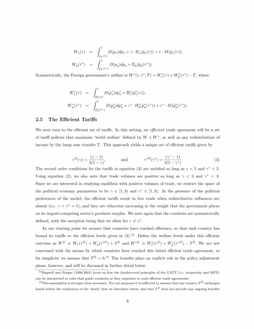
Wx(τ) =∫ 1

px(τ)

D(px)dpx + γ ·Πx(px(τ)) + τ ·M(px(τ)),

Wy(τ∗) =∫ 1

py(τ∗)

D(py)dpy + Πy(py(τ∗)).

Symmetrically, the Foreign government’s welfare is W ∗(τ, τ∗, T ) = W ∗x (τ) + W ∗

y (τ∗)− T , where

W ∗x (τ) =

∫ 1

p∗x(τ)

D(p∗x)dp∗x + Π∗x(p∗x(τ)),

W ∗y (τ∗) =

∫ 1

p∗y(τ∗)

D(p∗y)dp∗y + γ∗ ·Π∗y(p∗y(τ∗)) + τ∗ ·M(p∗y(τ∗)).

2.5 The Efficient Tariffs

We next turn to the efficient set of tariffs. In this setting, an efficient trade agreement will be a set

of tariff policies that maximize ‘world welfare’ defined by W + W ∗, as well as any redistribution of

income by the lump sum transfer T . This approach yields a unique set of efficient tariffs given by

τE(γ) =(γ − 1)2(5− γ)

, and τ∗E(γ∗) =(γ∗ − 1)2(5− γ∗)

. (3)

The second order conditions for the tariffs in equation (3) are satisfied so long as γ < 5 and γ∗ < 5.

Using equation (2), we also note that trade volumes are positive so long as γ < 3 and γ∗ < 3.

Since we are interested in studying equilibria with positive volumes of trade, we restrict the space of

the political economy parameters to be γ ∈ [1, 3) and γ∗ ∈ [1, 3). In the presence of the political

preferences of the model, the efficient tariffs result in free trade when redistributive influences are

absent (i.e. γ = γ∗ = 1), and they are otherwise increasing in the weight that the government places

on its import-competing sector’s producer surplus. We note again that the countries are symmetrically

defined, with the exception being that we allow for γ 6= γ∗.

As our starting point we assume that countries have reached efficiency, so that each country has

bound its tariffs to the efficient levels given in (3).14 Define the welfare levels under this efficient

outcome as WE ≡ Wx(τE) + Wy(τ∗E) + TE and W ∗E ≡ W ∗x (τE) + W ∗

y (τ∗E) − TE . We are not

concerned with the means by which countries have reached this initial efficient trade agreement, so

for simplicity we assume that TE = 0.15 The transfer plays an explicit role in the policy adjustment

phase, however, and will be discussed in further detail below.14Bagwell and Staiger (1999,2001) focus on how the fundamental principles of the GATT (i.e. reciprocity and MFN)

can be interpreted as rules that guide countries as they negotiate to such efficient trade agreements.15This assumption is stronger than necessary. For our purposes it is sufficient to assume that any nonzero T E exchanges

hands before the realization of the ‘shock’ that we introduce below, and that T E does not provide any ongoing benefits

8

2.6 Unilateral Policy Changes and their Welfare Effects

Before we discuss policy changes within the context of the GATT/WTO, it is illustrative to first

decompose by standard means the welfare effects of a unilateral tariff increase. Suppose Home raises its

tariff from its initial level, τE , to some nonprohibitive level τ1. The welfare effects of a non-prohibitive

tariff increase are illustrated in Figure 1 and can be broken down exhaustively as follows.

2.6.1 Terms of Trade Effect

When Home imposes a higher tariff, it shifts the terms of trade in its favor by driving down the price

that the Foreign exporters receive for good x. The result is a terms of trade gain to Home (given by

the black rectangle in panel a) and an equivalent terms of trade loss to Foreign (given by the striped

rectangle in panel b) of

12(τ1 − τE)(

12− τ1)

2.6.2 Offsetting Deadweight Losses

When Home increases its tariff, there are also associated deadweight losses. The sum of Home’s

traditional consumption and production distortion associated with the tariff increase (Home’s grey

shaded triangles in panel a of Figure 1) is equivalent to the deadweight loss imposed on Foreign (the

grey shaded triangle of panel b), given by

14(τ1 − τE)2.

2.6.3 Local Effects

The two remaining effects on welfare will be referred to jointly as the local effects as they only affect

the welfare of the policy changing (Home) country.

Politically-Weighted Producer Surplus Gain

When Home imposes a higher tariff, some of what was previously its consumer surplus is now

shifted to producer surplus, which is weighted more heavily in the government’s objective function.

The result is a gain (given by (γ − 1) multiplied by the black trapezoid of panel a) equivalent to

that one party might credibly threaten to take away from the other after the shock. This assumption is necessary because

we are interested in isolating an analysis on the GATT/WTO rules of tariff adjustments and tariff retaliation, and not

on the means by which countries might retaliate through non-tariff measures such as a threat to revoke any side benefits

captured in T E .

9

γ − 18

(τ1 − τE)(1 + τ1 + τE).

Additional Deadweight Loss Due to Lost Tariff Revenue

Finally, when Home starts from an initial positive tariff τE , there is another deadweight loss given

by a portion of lost tariff revenue. This additional deadweight loss is given graphically by the sum of

the small striped rectangles in panel a and is

τE(τ1 − τE).

2.6.4 Combining the Welfare Effects

Next let us combine the effects on Home and Foreign welfare that arise when Home imposes a higher

tariff on its imports of x. One means by which we can aggregate the effects that will simplify the

analysis that follows in the bargaining section is to consider the net welfare effect (Home effect minus

Foreign effect) of a tariff increase from τE to τ1, defined as follows

Ωx(τE , τ1) ≡ [Wx(τ1)−Wx(τE)]− [W ∗x (τ1)−W ∗

x (τE)] (4)

=[(τ1 − τE)(

12− τ1)

]+

γ − 1

8(τ1 − τE)(1 + τ1 − 9− γ

γ − 1τE)

.

The term in square brackets is twice the terms of trade effect (Home gain - Foreign loss), and the term

in curly brackets represents the local effect on welfare due to Home’s tariff increase in the x sector.

In a symmetric fashion we can define the net welfare effects that arise should Foreign raise its tariff

from τ∗E to some nonprohibitive τ∗1 as

Ωy(τ∗E , τ∗1) ≡ [W ∗y (τ∗1)−W ∗

y (τ∗E)]− [Wy(τ∗1)−Wy(τ∗E)] (5)

=[(τ∗1 − τ∗E)(

12− τ∗1)

]+

γ∗ − 1

8(τ∗1 − τ∗E)(1 + τ∗1 − 9− γ∗

γ∗ − 1τ∗E)

.

This is also the combination of twice the terms of trade effect (Foreign gain - Home loss) plus the local

effect on welfare due to Foreign’s tariff increase in the y sector.

10

2.7 Nash Bargaining and the Comparison of Threat Points

2.7.1 The Political Economy Shock

Recall that we begin our analysis under the assumption that countries have reached an initial efficient

agreement. In the following sections we consider how a country reacts when faced with a preference

‘shock’ that causes it to seek an adjustment to its trade policy away from the initial efficient level.

One motivation for this ‘shock’ is a country having elections and facing a new government in power

that prefers less trade than its predecessor. Perhaps the countries could not wait to sign the agreement

until after all elections were held due to a time constraint on the round of negotiations, for example,

imposed by the legislative time limit on the United State’s executive’s ‘fast-track’ authority.

Without loss of generality we assume that Home receives the shock to its political economy param-

eter. Let ε ≥ 0 be the size of the shock and define γ(γ, ε) ≡ γ + ε to be the level of Home’s political

economy parameter after the shock has been received. For simplicity we require that the ‘shock’ be

sufficiently small so that if γ < γ∗, then γ < γ∗ as well. First note that with the shock to the political

economy parameter, Home’s welfare is no longer WE . With the new political economy parameter,

define Home’s new transitional level of welfare as WT ≡ W (τE , τ∗E , γ). Foreign’s welfare is unchanged

and is still W ∗E . The shock then provides an efficiency reason for Home to ultimately implement a

new efficient tariff given by

τE(γ) ≡ (γ − 1)2(5− γ)

. (6)

2.7.2 Updating the Policy Change: Two Routes

We interpret the GATT/WTO system as having established two routes that Home can choose between

in eventually implementing the new efficient tariff when such trade policy adjustments are necessary

‘between rounds.’16 First, Home could proceed ‘legally’ by following the rules of the GATT/WTO’s

safeguards provisions. We assume that the process of legal implementation of protection requires (i)

that Home immediately update its tariff to the new efficient level, and (ii) that Home notify Foreign

of the tariff change so as negotiate compensation under the threat of sanctions determined by the

GATT/WTO rules on safeguards. On the other hand, Home could implement a new tariff ‘illegally.’

As we are not interested here in questions of uncertainty and monitoring, we assume that an illegal16We have greatly simplified the analysis by assuming that any policy adjustments take the form of tariff barriers,

neglecting consideration of quantitative restrictions, domestic policies and other non-tariff barriers which might lead

to ‘nonviolation nullification and impairment’ complaints. We address how it is that the model might be expanded to

include these additional issues in section 5.

11

tariff is detected instantaneously and with certainty, and that Home negotiates to the new efficient

outcome under the threat of Foreign sanctions as determined under the dispute settlement mechanism.

We model the illegal and legal routes as establishing two distinct fora which have two associated sets

of rules over the retaliatory tariff threats that Foreign is committed to using. We use the GATT/WTO

statutes to interpret and identify the levels of retaliation under each of the two routes. We then

assume that Home’s initial tariff (illegal or legal) and the associated Foreign retaliatory tariff threat

imply welfare benchmarks that serve as threat points used during the negotiations back to the efficiency

frontier. Instead of implementing a specific bargaining procedure, we use the Nash bargaining solution

and assume equal bargaining power across countries, in order to illustrate the negotiated outcome on

the efficiency frontier.17 Ultimately in this structure Home makes its protection-implementation choice

of which path to follow by simply comparing threat points.

Consider next the role of the transfer mechanism in the renegotiations phase. After the shock the

‘new’ efficient tariffs are uniquely determined by τE and τ∗E of (6) and (3), respectively. Therefore,

as illustrated in Figure 2, the assumptions generate a linear efficiency frontier determined by WE ≡

W (τE , τ∗E) and W ∗E ≡ W (τE , τ∗E), and the two countries are renegotiating over the size of a transfer,

T . Figure 2 also provides a pair of hypothetical threat points to provide intuition for our approach:

one threat point under the illegal route (I) and the other under the legal route (L). Assume that the

benchmark welfare levels at I and L are W I , W ∗I and WL, W ∗L, respectively, where the welfare

levels are to be determined by the illegal and legal sets of tariff changes that we formally identify

below. Given our assumptions, the equilibrium value for T in the renegotiations phase is determined

by the combination of the threat point of the chosen route and the position of the efficiency frontier.

As illustrated in Figure 2, if we identify WS,L as the final negotiated settlement (S) level of welfare

on the efficiency frontier that Home achieves under the legal route, the legal route transfer is simply

TL ≡ WS,L − WE . We calculate the value for TL explicitly below.

Before we proceed to a formal comparison of the threat points and a determination of Home’s equi-

librium protection implementation behavior as well as the equilibrium transfer, we pause to interpret

the role of the transfer at, for example, the conclusion of negotiations under the safeguards provisions.

Recall that our model assumes the existence of import policies only. We think of TL as substituting

for export policies in the model, allowing countries to transfer welfare directly, in lieu of redistributing17For a discussion of Nash bargaining in a general equilibrium trade model see Mayer (1981) or Riezman (1982).

Though our results are determined by relative power imbalances which refer to ‘weak’ and ‘strong’ countries, these

imbalances are determined by the interaction of the rules of the system and each country’s capacity to retaliate and

affect the terms of trade. A more general bargaining game with asymmetric bargaining powers across governments (and

perhaps even across statutes) would provide interesting additional insights.

12

rents through a restructuring of Home’s tariff into a Foreign VER. Ono (1991) has noted the economic

efficiency gains that arise when countries conclude compensation negotiations with a VER which has

one layer of efficiency losses and a transfer of rents, as opposed to two layers of efficiency losses, the

second of which would be due to a retaliatory tariff.18

Finally, while we often refer to Foreign’s retaliation in the discussion that follows, note that re-

taliation is only used to establish a threat point from which countries commence their compensation

negotiations. Ultimately countries do not retaliate and the outcome results in efficiency. Our interests

lie in the equilibrium path that countries choose in order to negotiate to the new efficiency frontier.19

2.7.3 Comparing the Threat Points

Since we are using the Nash bargaining solution to determine the negotiated equilibrium, we can make

this simple comparison of the threat points in Figure 2 with

Observation 1 Home will follow the illegal route if its threat point yields a better bargaining position,

i.e. if [W I − W ∗I ]− [WL − W ∗L] > 0.

But we can expand this algebraically and rewrite it for this general case as

[W I − W ∗I ]− [WL − W ∗L]

=[(W I − WT )− (W ∗I − W ∗E)

]−

[(WL − WT )− (W ∗L − W ∗E)

]=

[(W I

x − WTx ) + (W I

y −WEy )

−

(W ∗I

x − W ∗Ex ) + (W ∗I

y −W ∗Ey )

]−

[(WL

x − WTx ) + (WL

y −WEy )

−

(W ∗L

x − W ∗Ex ) + (W ∗L

y −W ∗Ey )

]=

[Ωx(τE , τ I)− Ωy(τ∗E , τ∗I)

]−

[Ωx(τE , τL)− Ωy(τ∗E , τ∗L)

]. (7)

Note first that after substituting γ for γ we replace (4) with

Ωx(τE , τ1) =[(τ1 − τE)(

12− τ1)

]+

γ − 1

8(τ1 − τE)(1 + τ1 − 9− γ

γ − 1τE)

, (8)

18However, for a discussion of the GATT-legality of voluntary export restraints see Jackson (1993).19While retaliation is permissible under the GATT, it has rarely been the ‘final outcome’ in practice, for the noted

efficiency reasons. Until the recent US v. EC Banana Regime and Beef/Hormone cases, no GATT/WTO dispute had

ever concluded with GATT/WTO sanctioned retaliation being implemented, and only in the 1951 Netherlands v. US

Dairy Quotas case was retaliation itself actually sanctioned (see Hudec, 1990, pp. 181-200). It would be misleading to

suggest, however, that retaliation is irrelevant because it is rarely carried out. It can be presumed that retaliation has

been threatened during negotiations and was GATT/WTO permissible much more frequently. For example, the GATT

reports 11 safeguards instances in which an affected country either cited Article XIX:3 or made a formal appeal for

retaliation (WTO, 1995, pp. 539-59).

13

where τ1 ∈ τL, τ I. We use (8) in the last step of (7) as well as Ωy(·), which is determined as it was

in (5). Therefore, we can restate Observation 1 as

Observation 2 Home will follow the illegal route if the associated net terms of trade and local effects

are larger than they are under the legal route, i.e. if [Ωx(τE , τ I) − Ωy(τ∗E , τ∗I)] − [Ωx(τE , τL) −

Ωy(τ∗E , τ∗L)] > 0.

In the following sections we add structure to Observation 2 by interpreting first how the GATT

(section 3) and now WTO (section 4) statutes determine the illegal (τ I , τ∗I) and legal (τL, τ∗L) tariff

combinations which, in turn, determine the benchmark threat points. After establishing the threat

points, we proceed to characterize the equilibria of the model.

3 The Rules under the GATT 1947

We focus in this section on interpreting the GATT 1947 rules of retaliation. In Section 4 we interpret

the Uruguay Round reforms and illustrate how these changes affect the rules of retaliation and thus

the qualitative nature of the results. We first look to formally determine the threat point that ensues

under the rules of the GATT if Home were to implement the protection ‘legally.’

3.1 The Legal Route and the Role of Reciprocity

The GATT-founders realized that governments face changing political economy pressures from their

private sectors that require a certain degree of flexibility with respect to their international obligations.

As previously discussed, there are many areas of the GATT including Articles XIX and XXVIII under

which countries are permitted to alter their tariff bindings without fear that the entire agreement will

fall apart.20 With respect to these safeguards measures, the GATT authorizes a Foreign country that

has been affected by Home’s tariff increase to (at least threaten to) obtain compensation through a

limited retaliation in which it imposes additional protection for its import-competing sectors. If Home

legally alters its trade policy, the language of the GATT 1947 implies that Foreign may not retaliate

beyond the point where it withdraws substantially equivalent concessions.21

20While Articles XIX and XXVIII are not perfect substitutes as Article XIX also has a “serious injury” provision,

Jackson (1989, p. 165) notes that meeting such requirements was usually “abused or ignored” and rarely challenged.21See Article XIX: 3(a) for temporary measures and Article XXVIII: 3(b) for permanent modifications of tariff bindings.

Furthermore, unlike the case of Article XXIII which we will discuss below, the reciprocity limit on retaliation under these

safeguards provisions was arguably policed by the GATT. For example, the 1978 Panel Report on Lead and Zinc (see

Pescatore et al., 1995, pp. 165-168) involved a case between the EC and Canada over the level of permissible retaliation

by Canada in response to an EC Article XXVIII modification of its tariff binding.

14

Suppose therefore that Home chooses to use the safeguards provisions. With a change in its political

economy parameter to γ, we define Home as proceeding ‘legally’ by assuming that the safeguards

provisions require Home to notify the GATT that it wishes to increase its tariff directly from τE ,

given by equation (3), to its new efficient level, τE , given by equation (6).22 Following the definition

of Bagwell and Staiger (2001),23 we say that given a set of tariffs τE , τ∗E, a second set of tariffs

τE , τ∗R is defined as balancing substantially equivalent concessions (or satisfying the condition of

reciprocity) if the proposed tariff change brings about equal changes in the volume of each country’s

imports and exports, when valued at existing world prices.24 That is, Bagwell and Staiger have shown

that this definition implies that the tariff pairs then satisfy the following condition

[pwx (τE)− pw

x (τE)]M(τE) = [pwy (τ∗E)− pw

y (τ∗R)]M∗(τ∗R), (9)

where τ∗R is the Foreign reciprocity tariff. But comparing equation (9) to Figure 1, we can make

Observation 3 The Foreign retaliatory tariff that satisfies the reciprocity condition will serve to neu-

tralize the terms of trade effect induced by Home’s original tariff increase.

Rather than solve for an explicit formula for the Foreign reciprocity tariff, it is sufficient to charac-

terize its important properties. If we define Home’s tariff change and Foreign’s retaliatory response as

τE = τE + ∆ and τ∗R = τ∗E + ∆∗, respectively, then we can rewrite (9) as

12(∆)

[12− τE −∆

]=

12(∆∗)

[12− τ∗E −∆∗

]. (10)

Clearly if τE = τ∗E , then ∆ = ∆∗ and τ∗R = τE , and equation (10) indicates that under symmetry

(when γ = γ∗), Foreign’s reciprocity response will be identical to the original Home tariff increase.

But if τE 6= τ∗E , then we note the following25

22We do not consider a setting whereby Home solves for some optimal legal tariff given the reciprocity condition. We

assume that the rules require that Home directly implement its new efficient tariff, and then the negotiations under the

safeguards provisions concern the size of the transfer determined by the Foreign reciprocity tariff response and the Nash

bargaining procedure. The efficiency and distributional properties of such a rule are explored in more detail below.23A discussion of reciprocity in the GATT as it applies to renegotiations of tariff bindings can be found in Dam (1970,

pp. 87-91). See also Bagwell and Staiger (1999).24Referring again to the general equilibrium interpretation of the model, the reciprocity condition is defined as

pwx (τE)[M(τE) − M(τE)] + Mz(τE , τ∗R) − Mz(τE , τ∗E) = pw

y (τ∗E)[M∗(τ∗R) − M∗(τ∗E)].

where Mz denotes Home imports of z. We then proceed in two steps. First, eliminate existing trade volumes from this

condition by utilizing the requirement of balanced trade at the existing set of world prices. Second, use the requirement

of balanced trade at the proposed tariffs set of world prices to eliminate trade in the numeraire good under the proposed

tariff. Given these two conditions, the definition of reciprocity implies the condition found in (9).25The proofs of all Propositions are found in the Appendix.

15

Proposition 1 If Home’s initial efficient tariff is larger (smaller) than Foreign’s, then when Home

increases its tariff, Foreign must make a proportionately smaller (larger) tariff increase in order for

the reciprocity condition to be satisfied. That is, ∂∆∗/∂τE < 0.

This result has direct implications of consequent importance. Specifically, note that τ∗R has the

following properties

Corollary 1 If γ < γ∗, then (τE − τE) < (τ∗R − τ∗E), and if γ > γ∗, then (τE − τE) > (τ∗R − τ∗E).

In reference to Figure 2, so long as τ∗R 6= τ∗E , any legal threat point L which is now determined

by the pair τE , τ∗R will be strictly interior to the new efficiency frontier so that both countries can

be made better off by negotiating a settlement under which they reach the frontier.

Finally, it is important to note that we are assuming that Foreign is also committed to only re-

sponding with its reciprocity tariff, τ∗R, when Home changes its tariff policy under the safeguards

provisions. We return to a discussion of this assumption in section 3.3.2.

3.2 The Illegal Route and Dispute Settlement

Article XXIII of the GATT 1947 was the forum to which countries brought complaints that trading

partners had undertaken policies which either violated GATT rules or nullified or impaired benefits

that trading partners had expected to receive under the Agreement. In either case, Article XXIII

allowed for countries affected by these measures to seek compensation through retaliation. Is the level

of retaliation that a country might face under Article XXIII truly different from that which it might

confront under the safeguards provisions? We argue in the affirmative, and our structure rests entirely

on this assumption. We use the rest of this section to argue in support of this distinction.26

To address this issue we consider two different arguments made by legal scholars. First, one could

take the position that limits on the level of permissible retaliation under Article XXIII were never

adequately defined. In fact, in reference to the 1951 Dairy case discussed earlier, Hudec notes that

during the dispute “[t]he Contracting Parties had brought out their biggest guns against the dominant

partner [the US]. They had threatened everything that could be threatened, including the collapse

of the Agreement itself.” (Hudec, 1990, p. 184). In this early GATT dispute, the retaliation threat

reached the level of the breakdown of the entire set of established rules. We assume that the “collapse

of the Agreement” would be followed by countries implementing nationally optimal (Nash) policies.

Alternatively, other scholars have argued that the statute did limit the level of permissible retaliation

in a trade dispute, it was simply that this level was not monitored. Roessler et al. have argued along26One clear way in which they are different is the language across the statutes. While both Article XIX and Article

XXVIII us the phrase substantially equivalent concessions, Article XXIII:2 contains the distinct such concessions clause.

16

these lines, stating that “Article XXIII nominally put a constraint on the magnitude of ‘damages,’ [i.e.

retaliation,] but there was no satisfactory mechanism for reviewing them and thus nations aggrieved

by violations could threaten or even impose damages out of proportion to the harm that they had

suffered.” (Roessler et al., forthcoming, emphasis added). In this case, we assume that if left un-

monitored, countries could threaten to implement nationally optimal (Nash) retaliatory policies.

Taking either of these perspectives leads us to conclude that a country could face the threat of a

more substantial retaliation under a policy which led to a trade dispute than it could face if it had

proceeded legally under either Article XIX or XXVIII. We now turn to a consideration of the modeling

implications of this assumption.

3.2.1 Trade Policies and Retaliation under the Illegal Route

In the context of our model, we focus on Article XXIII as the forum for countries to obtain compensation

for their trading partners’ ‘illegal’ changes in trade policy. Based on our arguments of the previous

section, we interpret the ‘rules’ (or perhaps the lack of well-defined rules) of the GATT’s dispute

settlement mechanism as imposing no binding constraint on the level of retaliation that an affected

Foreign country could threaten.27

With no external binding constraint, in recognition of the negotiations phase that would follow,

we assume that Foreign threatens to respond with its Nash tariff, or the tariff that would serve to

unilaterally maximize its objective function, W ∗. In recognition of this policy response and with the

similar intention of putting itself in an advantageous bargaining position for the negotiations to follow,

if Home were to decide to implement the protection ‘illegally’ in the first place, we assume that it would

proceed by increasing its tariff to the Nash level.28 Therefore, we can work through each country’s

best response function and solve for the set of Nash tariffs yielding

τN (γ) =γ + 1

2(7− γ), and τ∗N (γ∗) =

γ∗ + 12(7− γ∗)

. (11)

27As suggested, this assumption is not without controversy, though we do explore the sensitivity of our results to

changes in this assumption in section 4 below. Note also that throughout the analysis we do not consider the fact that

under the GATT regime each country had a veto-power in which it could essentially block any panel report that might

sanction retaliation. We assume that even in such cases, countries could still threaten retaliation either outside of Article

XXIII negotiations, or as a last resort, perhaps through threats of the “collapse of the Agreement.”28This approach is broadly consistent with the statements of the previous section, where we interpret threats as to

the “collapse of the Agreement” as countries reverting to Nash tariff policies. An alternative ‘credible’ threat could be

the reversion to autarky, though we consider this threat to be less relevant to the context presented here. We provide a

discussion of other potential policies (in the context of how they relate to trade disputes) aside from Home’s Nash import

tariff in the conclusion.

17

The second order conditions for the tariffs given in equation (11) are satisfied and the Nash tariffs are

nonprohibitive given the parametric restrictions already imposed. Note that for γ, γ∗ ∈ [1, 3) the Nash

tariffs are always positive, as the terms of trade gain is larger than the efficiency loss associated with

the reduction in imports. We note as well that

Observation 4 The difference between Home’s (Foreign’s) Nash and efficient tariffs is maximal when

the political economy weight is one, and it decreases monotonically until it is smallest, i.e. the tariffs

are equivalent, when the tariffs become prohibitive at γ = 3 (γ∗ = 3).

Again, we reiterate that there is no uncertainty or observational delay in the model. Ours is not a

dynamic model where Home ‘defects’ in order to achieve periods where it reverts to its Nash tariff and

time passes before this is observed and Foreign is permitted to retaliate. We obtain our basic results

even with the assumption that no time passes between when Home implements its illegal tariff and

when Foreign is authorized to retaliate. Home’s illegal tariff and Foreign’s retaliatory tariff establish a

threat point from which the countries immediately engage in Nash bargaining back to efficiency. Thus,

if Home were to choose the illegal route so that both it and Foreign implement their Nash tariffs, the

Nash threat point after the political economy shock would serve as point I in Figure 2. We now turn

to a characterization of the equilibria of the model.

3.3 Characterizing the Equilibria

Home’s choice of whether to implement protection legally or illegally is dependent on the relationship

between the two threat points established in the prior sections. Given that we have now established

the legal and illegal tariffs under the GATT as τL = τE , τ∗L = τ∗R, τ I = τN and τ∗I = τ∗N , we can

now restate Observation 2 as

Observation 5 Home will follow the illegal route if [Ωx(τE , τN ) − Ωy(τ∗E , τ∗N )] − [Ωx(τE , τE) −

Ωy(τ∗E , τ∗R)] > 0.

And we can characterize our first substantive result with

Proposition 2 If γ∗ ≥ γ then Home will choose the illegal route and implement protection by circum-

venting the GATT rules, leading to a trade dispute. However, if γ∗ < γ then a shock will cause Home

to implement protection legally under the GATT’s safeguards provisions.

While we relegate the formal proof to the appendix, we discuss here the intuition behind the result.

Consider Observation 5, equations (8) and (5), and the definitions of the tariffs, as these are the factors

that serve to affect the welfare levels of the threat points in the model.

18

Under the legal route, by definition of the Foreign reciprocity tariff (see Observation 3), the terms

of trade effects induced by the tariff changes in the x and y sectors would cancel, so we are simply left

with the local effects. However, under the illegal route we must contend with the local effect and the

terms of trade effect. Consider Figure 3 which illustrates the size of (twice) the terms of trade effect as

well as the local effects of Ωx and Ωy of equations (8) and (5), as a function of the political economy

parameters under the illegal route for Home (panel a) and Foreign (panel b). Clearly the terms of

trade effect dominates the local effect in absolute terms for political economy weights that are not too

large.29 Thus with any asymmetry in political economy weights, the country with the lower political

economy weight will also have the dominant terms of trade effect.

Since Home chooses which route to take, if it were the country with the relatively low political

economy weight (e.g. take γA and γ∗A in Figure 3) it will take advantage of its dominant terms of trade

effect by utilizing the illegal route. If Foreign has the lower weight (i.e. take the pair γB and γ∗B) then

Home will avoid the illegal route and the threat of the terms of trade loss imposed by Foreign, and it

will choose the legal route instead.

To further develop the intuition behind this result, note how varying the political economy param-

eter levels affect certain features of the model. First, combining (3) with equation (1) yields

ME ≡ M(px(τE(γ))) =3− γ

5− γand EE ≡ E(py(τ∗E(γ∗))) =

3− γ∗

5− γ∗. (12)

Equation (12) and the fact that ∂EE/∂γ∗ < 0 can be seen to provide support for Dam’s (1970) point:

a high γ∗ would imply that Foreign “does not consume enough of [Home’s]...exports...” to be able

to shift the terms of trade by an amount that is sufficient to induce Home into proceeding legally.

Suppose furthermore that γ < γ∗. By equation (3), under the original efficient agreement, Foreign’s

tariff bindings are already relatively high and by equations (3) and (12), a low γ implies that Home has

low bindings and large pre-shock imports of x from Foreign. By using the illegal route and its Nash

tariff, Home capitalizes on its own large imports and low initial efficient tariff to shift the terms of trade

and put itself in an advantageous bargaining position. Thus trade disputes occur when ‘strong’ Home

countries implement illegal policies that affect weaker trading partners who are relatively powerless in

their ability to threaten retaliation in compensation negotiations.

Suppose on the other hand that γ > γ∗. Then via the equations in (3) we have the opposite result:

high (low) values of γ (γ∗) imply that Home (Foreign) has high (low) tariff bindings. By equation (12)

Home (Foreign) imports are small (large). By Home choosing the legal route, it prevents Foreign from

threatening retaliation with its Nash tariff thereby avoiding a potentially large terms-of-trade loss in29Note that by (8) and (5) the legal local effects are smaller than the illegal local effects as τE < τN and τ∗R < τ∗N .

19

the y sector. Since Home’s efficient tariff is already high and relatively close to its Nash tariff (see

Observation 4) and its import volume is small, any terms-of-trade gains through Nash reversion in the

x sector would be limited. Thus ‘weak’ Home countries protect themselves by using the safeguards

provisions to limit the retaliation of their ‘strong’ trading partners to reciprocity compensation.

Another perspective on this result is to consider how a Home country with given political preferences

proceeds when faced with protection-implementation decisions and Foreign trading partners who are

differentiated by their γ∗ parameter. Proposition 2 thus suggests that Home will proceed illegally with

its most political trading partners and legally with the least political partners.

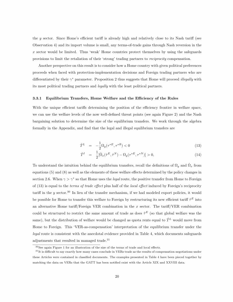
3.3.1 Equilibrium Transfers, Home Welfare and the Efficiency of the Rules

With the unique efficient tariffs determining the position of the efficiency frontier in welfare space,

we can use the welfare levels of the now well-defined threat points (see again Figure 2) and the Nash

bargaining solution to determine the size of the equilibrium transfers. We work through the algebra

formally in the Appendix, and find that the legal and illegal equilibrium transfers are

TL = −12Ωy(τ∗E , τ∗R) < 0 (13)

T I =12[Ωx(τE , τN )− Ωy(τ∗E , τ∗N )] > 0, (14)

To understand the intuition behind the equilibrium transfers, recall the definitions of Ωy and Ωx from

equations (5) and (8) as well as the elements of these welfare effects determined by the policy changes in

section 2.6. When γ > γ∗ so that Home uses the legal route, the positive transfer from Home to Foreign

of (13) is equal to the terms of trade effect plus half of the local effect induced by Foreign’s reciprocity

tariff in the y sector.30 In lieu of the transfer mechanism, if we had modeled export policies, it would

be possible for Home to transfer this welfare to Foreign by restructuring its new efficient tariff τE into

an alternative Home tariff/Foreign VER combination in the x sector. The tariff/VER combination

could be structured to restrict the same amount of trade as does τE (so that global welfare was the

same), but the distribution of welfare would be changed as quota rents equal to TL would move from

Home to Foreign. This ‘VER-as-compensation’ interpretation of the equilibrium transfer under the

legal route is consistent with the anecdotal evidence provided in Table 4, which documents safeguards

adjustments that resulted in managed trade.31

30See again Figure 1 for an illustration of the size of the terms of trade and local effects.31It is difficult to say exactly how many cases conclude in VERs trade as the results of compensation negotiations under

these Articles were contained in classified documents. The examples presented in Table 4 have been pieced together by

matching the data on VERs that the GATT has been notified exist with the Article XIX and XXVIII data.

20

On the other hand, when γ < γ∗ and Home uses the ‘illegal’ route, it receives an equilibrium

transfer from Foreign equal to T I of (14). Again referring to equations (5) and (8), in the illegal

case the size of the transfer is the difference between the Home and Foreign tariff-induced terms of

trade effects plus the difference between half the Home and Foreign tariff-induced local effects of their

Nash policies. A realistic interpretation of an equilibrium transfer from Foreign to Home that occurs

in actual trade disputes is the welfare gain that Home receives by the GATT (i) permitting Home a

period of time to bring its GATT-inconsistent policy into conformity, and (ii) not allowing Foreign to

retaliate in this interim period.

Consider next the efficiency of these rules of retaliation. We have not yet addressed the question

of whether or not these rules on ‘between rounds’ policy adjustments and retaliation responses under

the legal and illegal routes actually induce countries to update their trade policies to the new, efficient

level. Therefore, suppose we assume that Home has the option of not adjusting its trade policy after

receipt of the initial shock, would it choose to do so? Recall the alternative is Home’s transitional level

of welfare given by WT = W (τE , τ∗E , γ).

Clearly if Home is ‘powerful’ in the sense that it would use the illegal route in equilibrium, the

answer to this question is trivial as the illegal route yields to Home a positive transfer (T I) in addition

to the efficient level of welfare it achieves from updating its trade policy, where W (τE , τ∗E , γ) > WT

by the definition of τE . However, the answer to this question is not obvious with respect to a ‘weak’

Home country’s potential equilibrium use of the safeguards provisions. When γ > γ∗ would Home

actually utilize the ‘legal route’ in practice, even though we have found that under the safeguards

provisions it pays Foreign an equilibrium transfer? Does the reciprocity requirement of the legal route

induce efficient behavior, or does the requirement of compensation deter Home from updating its trade

policy and remaining at the (newly inefficient) τE? We conclude this discussion with the following

Proposition 3 The GATT rules induce efficient behavior. Even when γ > γ∗ Home is better off

having followed the legal route than it would have been by not responding to the shock and remaining

with the newly inefficient tariff τE and the transitional level of welfare WT .

3.3.2 The Rules on Safeguards and the Foreign ‘Welfare Compromise’

In terms of Foreign welfare, we can show that Foreign is worse off relative to W ∗E , i.e. its pre-

shock level of welfare. However, to understand an additional (distributional) motive for the safeguards

provisions, it is instructive to consider a thought experiment in which we contrast these results with

an alternate set of rules for ‘policy-updating.’ Suppose Home could simply update its trade policy to

the new efficient tariff without having to negotiate any compensation with Foreign.

21

The Legal Route

First consider the legal route. With the ‘no-compensation’ thought experiment determining the

third level of welfare, the ordering from Foreign’s perspective would be

W ∗(τE , τ∗E) > W ∗(τE , τ∗E)− TL > W ∗(τE , τ∗E)

Since TL < 0 (an equilibrium transfer from Home to Foreign) the safeguards provisions under the

GATT can be interpreted as a welfare compromise from the perspective of Foreign. When Home uses

the legal route, Foreign is clearly not as well off as it is would have been had Home not updated its

tariff at all. However, if we make the assumption that a role for the GATT is to generate rules which

create incentives for countries to update their policies to efficient levels, we can interpret the safeguards

provisions as at least providing Foreign with more welfare than it would have received had Home been

able to update its tariff to the new efficient level without having to yield any compensation.

However, one potentially troubling matter that we have not yet addressed is the assumption that

there is an external enforcement mechanism that compels Foreign to respond with its reciprocity tariff

when a ‘weak’ Home country uses the legal route in equilibrium. Whenever a ‘weak’ Home country

proceeds legally, Foreign would clearly prefer to respond with its Nash tariff, which would then pre-

sumably move the negotiations away from the safeguards provisions and into the dispute settlement

forum where, because γ > γ∗, Foreign would have a more favorable bargaining position.

We motivate this assumption by appealing to our discussion of the welfare compromise. We have

essentially assumed that Home and Foreign have agreed to a set of rules whereby each trades away the

right to respond illegally if the other initiates a policy change legally. In exchange, the countries agree

to abide by the efficiency-enhancing rule of reciprocity compensation which leads, as we have noted, to

the welfare compromise. We claim that the reciprocity rule is efficiency-enhancing by considering what

would transpire in the absence of such a rule. If countries had not agreed to those rules and there were

nothing to constrain Foreign from a Nash response when Home acted legally, a ‘weak’ Home country

would simply avoid the safeguards provisions altogether. Home would not, however, implement its

new, efficient tariff by proceeding illegally. In fact, the transfer under the illegal route, T I , is negative

when γ > γ∗ by (14), and we can show that a ‘weak’ Home achieves a higher level of welfare by not

updating its policy at all. Therefore, without a constraint on Foreign retaliation under the legal route,

GATT rules would not induce efficient policy updating by ‘weak’ Home countries.32

32Alternatively, we could appeal to the notion of “international obligation” of Kovenock and Thursby (1992), which

we could assume in this context to be a sizable cost that Foreign would face for implementing additional protection in

the absence of a shock. Both approaches admittedly point to a shortcoming of a framework which abstracts from the

issues of enforcement. We address this issue further in section 5.

22

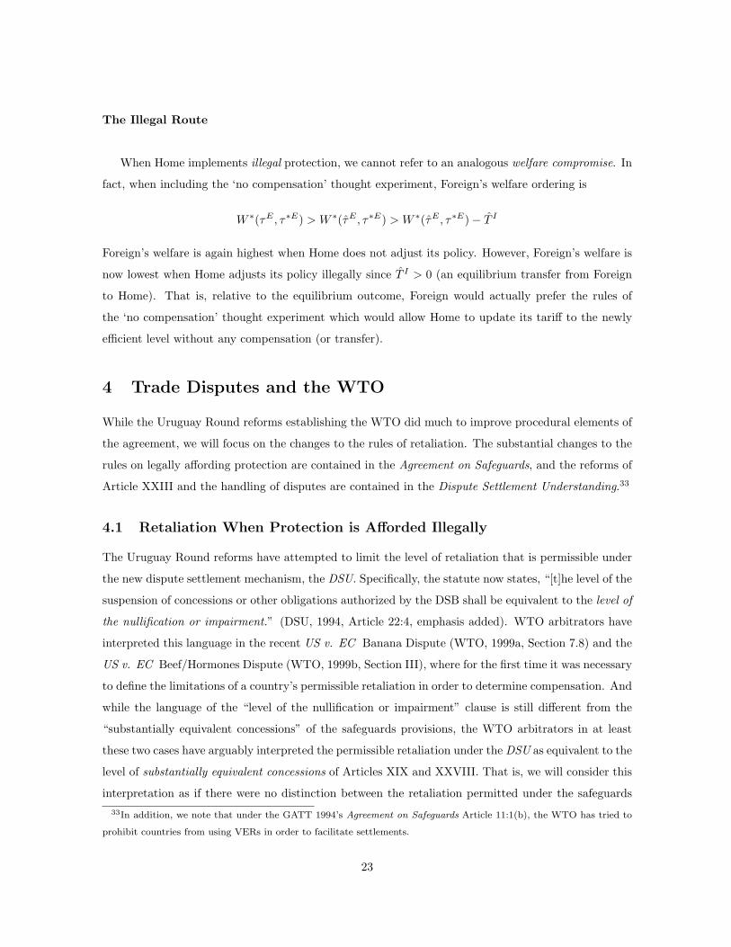
The Illegal Route

When Home implements illegal protection, we cannot refer to an analogous welfare compromise. In

fact, when including the ‘no compensation’ thought experiment, Foreign’s welfare ordering is

W ∗(τE , τ∗E) > W ∗(τE , τ∗E) > W ∗(τE , τ∗E)− T I

Foreign’s welfare is again highest when Home does not adjust its policy. However, Foreign’s welfare is

now lowest when Home adjusts its policy illegally since T I > 0 (an equilibrium transfer from Foreign

to Home). That is, relative to the equilibrium outcome, Foreign would actually prefer the rules of

the ‘no compensation’ thought experiment which would allow Home to update its tariff to the newly

efficient level without any compensation (or transfer).

4 Trade Disputes and the WTO

While the Uruguay Round reforms establishing the WTO did much to improve procedural elements of

the agreement, we will focus on the changes to the rules of retaliation. The substantial changes to the

rules on legally affording protection are contained in the Agreement on Safeguards, and the reforms of

Article XXIII and the handling of disputes are contained in the Dispute Settlement Understanding.33

4.1 Retaliation When Protection is Afforded Illegally

The Uruguay Round reforms have attempted to limit the level of retaliation that is permissible under

the new dispute settlement mechanism, the DSU. Specifically, the statute now states, “[t]he level of the

suspension of concessions or other obligations authorized by the DSB shall be equivalent to the level of

the nullification or impairment.” (DSU, 1994, Article 22:4, emphasis added). WTO arbitrators have

interpreted this language in the recent US v. EC Banana Dispute (WTO, 1999a, Section 7.8) and the

US v. EC Beef/Hormones Dispute (WTO, 1999b, Section III), where for the first time it was necessary

to define the limitations of a country’s permissible retaliation in order to determine compensation. And

while the language of the “level of the nullification or impairment” clause is still different from the

“substantially equivalent concessions” of the safeguards provisions, the WTO arbitrators in at least

these two cases have arguably interpreted the permissible retaliation under the DSU as equivalent to the

level of substantially equivalent concessions of Articles XIX and XXVIII. That is, we will consider this

interpretation as if there were no distinction between the retaliation permitted under the safeguards33In addition, we note that under the GATT 1994’s Agreement on Safeguards Article 11:1(b), the WTO has tried to

prohibit countries from using VERs in order to facilitate settlements.

23

provisions of the GATT 1947 and the illegal route of the WTO’s DSU.34 While this was not the only

change in the rules of retaliation under the WTO, it is instructive to first consider the implications as

if this were the only change.

4.1.1 DSU Reciprocity and the Model

Whereas we modeled the GATT’s dispute settlement as if there were no limit on retaliation, under the

DSU we now interpret an affected country’s permissible retaliation as being the suspension of trade

that is designed to stabilize the value of export and import trade volumes between countries, as in

equation (9). To make a consistent comparison with our earlier results, we again assume that Home

raises its tariff under the illegal route to τN . In this case, Foreign is only be permitted to raise its tariff

to the DSU tariff, τ∗DSU , implicitly defined in the reciprocity condition

[pwx (τE)− pw

x (τN )]M(τN ) = [pwy (τ∗E)− pw

y (τ∗DSU )]M∗(τ∗DSU ). (15)

First, this condition will be non-binding if γ < γ∗. We have already shown (see Figure 3) that Foreign

will not be able to offset Home’s terms of trade effect even with its Nash tariff, if Home has a smaller

political economy weight than Foreign. If γ < γ∗, Foreign will simply retaliate with its Nash tariff and

the terms of trade and local effects are determined just as they were in Observation 5.35

However, if γ > γ∗, then the reciprocity condition binds and Foreign will only be permitted a

retaliation that serves to neutralize the terms of trade effects as detailed in equation (15). From the

properties derived from Proposition 1 we note that this has the following implications

Corollary 2 If γ > γ∗, then (τN − τE) > (τ∗DSU − τ∗E).

Given that the legal and illegal tariffs under the WTO and under this set of parameter conditions are

τL = τE , τ∗L = τ∗R, τ I = τN and τ∗I = τ∗DSU , we can now restate Observation 2 in this case as

Observation 6 If γ > γ∗, Home will follow the illegal route if [Ωx(τE , τN ) − Ωy(τ∗E , τ∗DSU )] −

[Ωx(τE , τE)− Ωy(τ∗E , τ∗R)] > 0.

Finally, we can summarize the implications of this section with

Proposition 4 In the absence of any other changes, the DSU constraint on Foreign retaliation would

influence Home to always implement its protection changes illegally, leading to a dispute.34Without external enforcement, however, there will always be the implicit threat of the “collapse of the Agreement.”35Foreign would never credibly threaten to raise its tariff above τ∗N as any increase above this level would be welfare-

reducing relative to τ∗N . Second, note that we also do not consider a setting where Home solves for some optimal illegal

tariff given the DSU condition of (15).

24

Again while the proof is relegated to the Appendix, we discuss the intuition here. Clearly for γ ≤ γ∗

we have the same result (and intuition) as was previously the case under the GATT and was discussed

in Section 3.3. Since Home and Foreign both implement their Nash tariffs under the illegal route,

Home’s terms of trade effect would dominate and it would hence prefer the illegal route.

When compared to the GATT system described earlier, the incentives have changed when γ > γ∗.

Under the WTO, Foreign’s retaliatory tariff is binding below its Nash level and, by its definition, the

terms of trade effects under the illegal route are neutralized, just as they are under the legal route as

well. This constrains Foreign’s retaliation when compared to the GATT regime, where it would have

had the dominant terms of trade effect (with γ > γ∗), the threat of which thus induced Home into

proceeding legally. With the neutralized terms of trade effects, we can then show that the remaining

local effects are larger for Home under the illegal route.

4.2 Retaliation when Protection is Afforded Legally

The reform of the WTO rules of retaliation under the DSU were not the only changes to the GATT

system. While the WTO rules have made the level of permissible DSU retaliation essentially equivalent

to the level that affected countries were limited to under the legal route of the GATT 1947, the

level of permissible retaliation facing countries who implement protection under the Agreement on

Safeguards has also been modified. When a WTO Member country utilizes the escape clause to raise

its tariff on imported goods, its trading partners are still free to threaten the withdrawal of substantially

equivalent concessions.36 However, the statute forces affected trading partners to restrain from seeking

compensation until three years have passed since the original safeguard measure was put in place.37 We

interpret this rule change as attempting to make the safeguards provisions a more attractive alternative

to protection-affording Home countries, relative to the use of ‘illegal’ policy adjustments.

4.2.1 Analyzing the Safeguards Reforms

In considering the effects of these WTO reforms, we illustrate the changes by placing a µ ∈ [0, 1]

parameter on Foreign welfare under the legal route. Therefore, the combination of welfare effects

under the illegal and legal route is now

[Ωx(τE , τN )− Ωy(τ∗E , τ∗)]− [Ωx(τE , τE)− µ · Ωy(τ∗E , τ∗R)],

36See Agreement on Safeguards (1994) Article 8:2. Many additional revisions were also undertaken in order to provide

stricter standards to the injury test and specific time limits on the process. We do not address those issues here and

instead focus purely on the level of compensation due to affected countries.37Specifically the statute states, that “[t]he right of suspension...shall not be exercised for the first three years that a

safeguard measure is in effect...” (AS, 1994, Article 8:3, emphasis added).

25

where τ∗ ∈ τ∗DSU , τ∗N, just as was discussed in Section 4.1.1. If µ = 1, we have the results of

the GATT 1947 system, Proposition 4, and importantly, the continued Article XXVIII case where

compensation is still necessary. On the other hand, setting µ = 0 is equivalent to focusing on the other

extreme, under the assumption that Home does not compensate Foreign if it follows the legal route.

For illustrative purposes that is the case that we will consider here.

Thus consider the case that µ = 0, and note again that if γ < γ∗ the DSU constraint does not

bind and Foreign retaliates under the illegal route with its Nash tariff. However, if γ > γ∗ the DSU

constraint binds and Foreign retaliates under the illegal route with the tariff implicitly defined by

equation (15). Building again from Observation 2, in this case we have that the legal and illegal tariffs

are τL = τE , τ∗L = τ∗E , τ I = τN and τ∗I = τ∗, so if we assume µ = 0 we can make the following

Observation 7 If γ < γ∗, Home will follow the illegal route if [Ωx(τE , τN )−Ωy(τ∗E , τ∗N )]−Ωx(τE , τE) >

0. If γ > γ∗, Home will follow the illegal route if [Ωx(τE , τN )− Ωy(τ∗E , τ∗DSU )]− Ωx(τE , τE) > 0.

We consider the effects that this has on the equilibrium with

Proposition 5 With µ = 0 indicating no Foreign retaliation under the legal route, there exists a γ∗

such that we have the following

• if γ ∈ [1, γ∗), Home would proceed illegally,

• if γ ∈ [γ∗, γ∗), Home would proceed legally, and

• if γ ∈ [γ∗, 3), Home would proceed illegally.

The intuition behind this result is more subtle than for the earlier cases. Again with γ < γ∗, Home’s

terms of trade effect dominates under the illegal route, and even though Home does not compensate

Foreign under the legal route, the legal terms of trade and local effects are still small relative to the

improved bargaining position that Home would be able to obtain when taking advantage of its dominant

terms of trade effect when it proceeds illegally. The result is again a trade dispute.

However, when γ ≥ γ∗ there are two more cases to consider. The Safeguards reform eliminate

Foreign compensation and improve Home’s bargaining position (relative to the net effects of the illegal

route), provided the two countries aren’t too asymmetric (i.e. provided γ ∈ [γ∗, γ∗)). Once Home’s

political economy weight crosses a threshold given by γ∗, the constraint on Foreign’s DSU tariff

dominates, and the incentives become such that Home finds it preferable for it to proceed illegally.

Finally, in terms of the equilibrium transfers that are generated in this context, first note that when

Home uses the legal route, because there is no compensation due, the transfer will be zero (i.e. for

26

γ ∈ [γ∗, γ∗) we have TL = 0). When Home utilizes the illegal route, just as in the GATT case, it will

extract a transfer from Foreign in the negotiations back to efficiency.38

4.3 Comparing the GATT and WTO Systems

Consider finally Figure 4. When compared to the GATT 1947 system (panel a.), the DSU constraint

which limits Foreign retaliation serves to weaken the potential threat facing a country which proceeds

illegally (panel b.). While the reforms contained in the Agreement on Safeguards limit the necessary

compensation under the legal route, this has only served to partially mitigate this effect (panel c.).

As the asymmetry between countries increases, the DSU constraint dominates the reforms to the legal

route, even with the elimination of all necessary compensation. The WTO reforms of the retaliatory

rules under the DSU and Agreement on Safeguards can be interpreted as having opposing effects on

the incentives facing countries that seek to make ‘between rounds’ trade policy adjustments.

We highlight this result, as researchers such as Messerlin (2000) have called for the next negotiating

round to consider reforms designed to make utilization of the safeguards provisions more appealing,

especially in light of the proliferation in the use of antidumping measures. Our results suggest that in

order to effectively induce countries to more frequently utilize the safeguards provisions, the WTO will

need to simultaneously address the rules of retaliation under the trading system’s dispute settlement

mechanism. An important alternative to use of the safeguards provisions are countries implementing

GATT/WTO-‘illegal’ policies. Rules which weaken the level of authorizable retaliation under the DSU

create a disincentive for countries to utilize the safeguards provisions.

5 Conclusion

This paper is a first attempt at providing a theory to illustrate a motive for countries to implement

GATT/WTO illegal trade policy adjustments that will knowingly lead to trade disputes. We model

the dispute settlement mechanism as establishing a forum in which countries who have implemented

an illegal trade policy negotiate with affected trading partners back to efficiency. Countries in need

of trade policy flexibility are given the choice of implementing protection illegally or legally, where, in

this second case, negotiations take place under the GATT/WTO’s safeguards provisions.

We have shown that a country implements protection illegally, leading to a trade dispute, when it

has the capacity to take advantage of its own terms-of-trade gains and when its trading partners do not

have the potential to impose terms-of-trade losses through retaliation. On the other hand, consider a38Under the illegal route, the equilibrium transfer when γ < γ∗ is equivalent to the level under the GATT, given by

(14). On the other hand, when γ ∈ [γ∗, 3) the transfer is T I = 1/2[Ωx(τE , τN ) − Ωy(τ∗DSU , τ∗N )] > 0.

27

country that seeks a change in policy over a small volume of imports that are already protected with

high tariffs. If the trade affects a partner who has the capacity to inflict damages through large changes

in the terms of trade, then the country will be more likely to implement the necessary protection legally

under the GATT/WTO safeguards provisions so as to avoid a dispute.39

Our model illustrates the WTO reforms as having altered the rules of retaliation on two fronts. First,

we interpret the DSU reforms which limit retaliation as weakening the GATT system’s disincentive

facing countries which proceed illegally. Second, the reforms to the safeguards provisions that limit

retaliation (or compensation) when a country proceeds legally does create an additional incentive for

countries to follow the rules. However, our results indicate that the net result is only a partial offset

of the effect induced by the DSU reforms, and therefore that the changes to WTO rules on retaliation

have done little to decrease the likelihood that ‘strong’ countries will proceed illegally.

This simplified approach is only a first step toward improving our understanding of the role of trade

disputes in the international system. Certainly terms of trade considerations are not the only factor

that can influence such policy decisions, as is evidenced by the fact that most trade disputes do not

result from illegal import tariffs, but instead from quantitative restrictions, subsidies, domestic policies

or other NTBs. One could extend the model to include these alternative policies as well as perhaps

time delays, the introduction of a cost for pursuing disputes, differences in bargaining powers across

countries, and a positive probability of escaping detection.

Next, our modelling approach also does not allow for retaliation through non-tariff barriers. One

example of NTB retaliation occurring in practice is Ecuador threatening to withdraw its TRIPs com-

mitments as a means of retaliating against the EC for its refusal to bring its Banana Regime into

compliance with its WTO obligations (WTO, 2001, p.6). This issue should also be explored in fu-

ture research. Nevertheless, it is our conjecture that the capacity for Foreign retaliation will remain a

significant factor in a country’s decision of how to proceed with ‘between rounds’ policy adjustments.

Finally, as we have noted earlier, we have deliberately abstracted from issues of enforcement in this

model. A next step would be to take this model and embed it into a dynamic model of self-enforcing

trade agreements, in order to better address the interaction between Jackson’s “rule integrity” and

“conciliation and negotiation” approaches to understanding dispute settlement.39Empirical support for this initial proposition can be found in Bown (2001), which studies how countries implemented

additional protection under the GATT 1947. The study utilizes a data set on the illegal and legal cases (broken down as

in Table 3) under Articles XXIII, XIX and XXVIII between 1973 and 1994.

28

Appendix

Note that we simplify notation in the following manner. In terms of the levels of welfare, for Home let

WE ≡ W (τE , τ∗E , γ), WN ≡ W (τN , τ∗N , γ), WR ≡ W (τE , τ∗R, γ), and WDSU ≡ W (τN , τ∗DSU , γ),and

for Foreign let W ∗E ≡ W ∗(τE , τ∗E), W ∗N ≡ W ∗(τN , τ∗N ), W ∗R ≡ W ∗(τE , τ∗R), and W ∗DSU ≡

W ∗(τN , τ∗DSU ). Second, whenever the initial efficient tariffs serve as the initial trade policy in (8) or

(5) we will rewrite these welfare effects as ΩNx ≡ Ωx(τE , τN ), Ω∗R

y ≡ Ωy(τ∗E , τ∗R), etc. For many of

the proofs it is useful to have the following alternative formulations of (8) and (5):

Ω1x = [(τ1 − τE)(

12− τ1)] +

ε

8(τ1 − τE)(1 + τ1 + τE) +

γ − 18

(τ1 − τE)2 (16)

Ω1x =

ε

8(τ1 − τE)(1 + τ1 + τE) + [(τ1 − τE)(

12− 9− γ

8τ1 − γ − 1

8τE)] (17)

Ω1y = [(τ∗1 − τ∗E)(

12− τ∗1)] +

γ∗ − 18

(τ∗1 − τ∗E)2 (18)

Ω1y = [(τ∗1 − τ∗E)(

12− 9− γ∗

8τ∗1 − γ∗ − 1

8τ∗E)]. (19)

Calculation of the Transfers under the GATT Equilibrium of Equations (13) and (14)

With the linear (with slope -1) efficiency frontier and the equal bargaining powers assumption

(implying a negotiations ‘path’ of slope +1 from the benchmark), calculation of the equilibrium level

of welfare at the conclusion of the negotiations is very straightforward. For Home, the final equilibrium

level of welfare under the illegal and legal routes’ settlement (S), respectively, can be shown to be

WS,I =12WE +

12[W ∗E + WN − W ∗N ]

WS,L =12WE +

12[W ∗E + WR − W ∗R]

Since Home’s (pre-transfer) welfare at the newly efficient set of tariffs is given by WE , the transfers

are T I = 12 [(WN − WE)− (W ∗N − W ∗E)] and TL = 1

2 [(WR − WE)− (W ∗R − W ∗E)] or expanding,

T I =12

[(WN

x − WEx )− (W ∗N

x − W ∗Ex )] + [(WN

y −WEy )− (W ∗N

y −W ∗Ey )]

TL =

12

[(WR

x − WEx )− (W ∗R

x − W ∗Ex )] + [(WR

y −WEy )− (W ∗R

y −W ∗Ey )]

But note that WR

x = WEx and W ∗R

x = W ∗Ex and by (8) and (5) we have the forms given in the text

T I =12[Ωx(τE , τN )− Ωy(τ∗E , τ∗N )]

TL =12[WR

y −WEy )− (W ∗R

y −W ∗Ey )] = −1

2Ωy(τ∗R, τ∗E).

29

Calculation of the Transfers under the WTO Equilibrium

With no compensation under the legal route in the WTO, TL = 0. Under the illegal route, the final

equilibrium level of welfare under the settlement (S) is different depending on whether γ < γ∗, where

the transfer would again be given by (14) or whether γ ∈ [γ∗, 3), in which case we follow the same

steps as above (except substituting τ∗DSU for τ∗N ) yielding T I = 12 [Ωx(τE , τN ) − Ωy(τ∗E , τ∗DSU )],

which is the form given in footnote 38.

Proof of Proposition 1

Using the implicit function theorem, we find that ∂∆∗/∂τE = −∆/( 12 − τ∗E − 2∆∗) < 0, provided τ∗E

is not too large. Q.E.D.

Proof of Proposition 2

Case (i) Claim: with γ ≤ γ∗ Home prefers the illegal route.

By Observation 5 this requires showing that [ΩNx −ΩN

y ]− [ΩEx −ΩR

y ] > 0. By definition of τ∗R, the

terms of trade effects under the legal route are neutralized by Observation 3. Applying this information

to (16) and (18), the welfare effects under the legal route can be rewritten as

ΩEx − ΩR

y =ε

8(τE − τE)(1 + τE + τE) +

γ − 1

8(τE − τE)2 − γ∗ − 1

8(τ∗R − τ∗E)2

(20)

By Corollary 1, (τE − τE) < (τ∗R − τ∗E), so the term in curly brackets in (20) is negative. Under the

illegal route, we can use (17) and (19) to rewrite [ΩNx − ΩN

y ] as

ΩNx − ΩN

y =ε

8(τN − τE)(1 + τN + τE) + (21)

(τN − τE)(

12− γ − 1

8τE − 9− γ

8τN

)− (τ∗N − τ∗E)

(12− γ∗ − 1

8τ∗E − 9− γ∗

8τ∗N

)

With γ ≤ γ∗ we have (τN−τE) > (τ∗N−τ∗E) by Observation 4 and τE > τE . It is then straightforward

to show that the term in curly brackets in (21) is nonnegative and the first term of (21) is larger than

the first term of (20), thereby proving the result.

Case (ii) Claim: with γ > γ∗ Home prefers the legal route.

By Observation 5 this requires showing that [ΩNx −ΩN

y ]−[ΩEx −ΩR

y ] < 0. By Corollary 1, (τE−τE) >

(τ∗R − τ∗E), so equation (20) is now positive. With respect to the illegal route, rewrite (21) as

30

ΩNx − ΩN

y = (τN − τE)([

3 + γ

8− 9− γ

8τE

]− 9− γ

8τN

)(22)

−(τ∗N − τ∗E)([

3 + γ∗

8− 9− γ∗

8τ∗E

]− 9− γ∗

8τ∗N

).

Since γ > γ∗, we can show that (τN − τE) < (τ∗N − τ∗E). It is then straightforward to show that the

second term in square brackets in (22) dominates the first term in square brackets provided that ε is

sufficiently small, so (22) is negative, proving the result. Q.E.D.

Proof of Proposition 3

This requires showing W (τE , τ∗E , γ) + TL > W (τE , τ∗E , γ), where TL is defined by (13). But note

that by (8) this implies that we will show that

W (τE , τ∗E , γ)−W (τE , τ∗E , γ) >12Ωy(τ∗E , τ∗R) (23)

The left-hand side of (23) is simply the change in Home welfare due to a unilateral increase in Home’s

tariff from τE to τE , which can be broken down into the components given in Section 2.6 (i.e. the

terms of trade effect, local effect and a third deadweight loss term that doesn’t ‘offset’ in this case).

Recall that Ωy(τ∗E , τ∗R) contains a term that is twice the terms of trade effect from an increase from

τE to τE , (by definition of τ∗R), so these terms would cancel from each side of (23) leaving

γ − 18

(τE − τE)[1 + τE − 9− γ

γ − 1τE

]− 1

4(τE − τE)2 >

12

[γ∗ − 1

8(τ∗R − τ∗E)2

]Working through some algebraic steps leaves us needing to show

[τE − τE ]

γ − 14

− 3− γ

4τE − 7− γ

4τE

>

(γ∗ − 1

8

)[τ∗R − τ∗E ]τ∗R − τ∗E (24)

But comparing the two sides of (24), we have 1 > (γ∗ − 1)/8 and [τE − τE ] > [τ∗R − τ∗E ] by γ > γ∗

and Corollary 1. With respect to the terms in curly brackets in (24), it is straightforward to expand

out the terms of the left-hand side and show that (γ−1)/4− (3− γ)/4τE− (7− γ)/4τE > (τE−τE),

and from there, again by Corollary 1 we have that (τE−τE) > (τ∗R−τ∗E), thereby proving the result.

Q.E.D.

Proof of Proposition 4

Case (i) Claim: with γ ≤ γ∗ Home prefers the illegal route.

31

For γ ≤ γ∗ the proof is identical to Proposition 2, since the DSU constraint does not bind.

Case (ii) Claim: with γ > γ∗ Home now also prefers the illegal route.

This requires showing that [ΩNx − ΩDSU

y ] − [ΩEx − ΩR

y ] > 0. By definition of τ∗R and τ∗DSU , the

terms of trade effects under both the legal and illegal routes cancel, so the welfare effects under the

illegal and legal routes can be rewritten, respectively, from (16) and (17) as

ΩNx − ΩDSU

y =ε

8(τN − τE)(1 + τN + τE) +

[γ − 1

8(τN − τE)2 − γ∗ − 1

8(τ∗DSU − τ∗E)2

](25)

ΩEx − ΩR

y =ε

8(τE − τE)(1 + τE + τE) +

[γ − 1

8(τE − τE)2 − γ∗ − 1

8(τ∗R − τ∗E)2

](26)

If we subtract (26) from (25) and do some algebra we get

[ΩNx − ΩDSU

y ]− [ΩEx − ΩR

y ] = ε

8(τN − τE)(1 + τN + τE)− ε

8(τE − τE)(1 + τE + τE)

+ (27)

γ − 18

(τN − τE)[(τN − τE) + (τE − τE)

]− γ∗ − 1

8(τ∗DSU − τ∗R)

[(τ∗DSU − τ∗E) + (τ∗R − τ∗E)

]

Clearly the term in curly brackets in (27) is positive. With regards to the other terms, with γ > γ∗, by

Corollary 2 (τN − τE) > (τ∗DSU − τ∗E), and by Corollary 1 (τE − τE) > (τ∗R− τ∗E). In order to show

that (τN − τE) > (τ∗DSU − τ∗R), subtract the left hand side (right hand side) of the DSU reciprocity

condition (15) from the left hand side (right hand side) of the GATT reciprocity condition (9) and

expand out the terms yielding

(τN − τE)[(

12− τN

)−

(τE − τE

)]= (τ∗DSU − τ∗R)

[(12− τ∗DSU

)−

(τ∗R − τ∗E

)](28)

Therefore, with γ > γ∗ we must have (τN − τE) > (τ∗DSU − τ∗R) in order for the equality of (28) to

hold. Thus (27) > 0 thereby proving the result. Q.E.D.

Proof of Proposition 5

Case (i) With γ < γ∗ Home prefers the illegal route.

Note then that τ∗ = τ∗N and let Λ ≡ [ΩNx − ΩN

y ]− ΩEx . Rearranging the elements of Λ yields

Λ = (τN − τE)[3 + γ

8− 9− γ

8τN − 9− γ

8τE

]− (τ∗N − τ∗E)

[3 + γ∗

8− 9− γ∗

8τ∗N − 9− γ∗

8τ∗E

](29)

32

To show that Λ > 0 from (29), recall that γ < γ∗ implies (τN − τE) > (τ∗N −τ∗E) from Observation 4.

It is then straightforward to show that the terms in the first square brackets are larger than those in

the second thereby proving the result.

Case (ii) With γ = γ∗ Home prefers the legal route.

In order to show that Λ < 0, note that since γ∗ = γ, (29) turns into

Λ = (τN − τE)[3 + γ

8− 9− γ

8τN − 9− γ

8τE

]− (τN − τE)

[3 + γ

8− 9− γ

8τN − 9− γ

8τE

](30)

With γ > γ, (τN − τE) < (τN − τE), and it is straightforward to show that the terms of the second

square brackets of (30) are larger than those of the first, showing that (30) < 0 and giving us the result.

Case (iii) There exists a γ∗ such that with γ ∈ [γ∗, γ∗) Home prefers the legal route, and γ ∈ [γ∗, 3)

Home prefers the illegal route.

Note here that the constraint binds so τ∗ = τ∗DSU . Now under the illegal route the terms of trade

effects cancel and Home proceeds legally if

[ΩNx − ΩDSU

y ]− ΩEx =

γ − 18

(τN − τE)[1 + τN − 9− γ

γ − 1τE

](31)

− γ∗ − 18

(τ∗DSU − τ∗E)2 − (τE − τE)[3 + γ

8− 9− γ

8τE − 9− γ

8τE

]< 0.

With no analytical formula for τ∗DSU we lack a formal means to characterize the last solution,

so we appeal to Figure 5. There we plot the three effects identified in equation (31) (the Home and

Foreign illegal local effects and the Home welfare effects of the legal route) as a function of γ and

γ∗. In panel a we consider the case for Home and Foreign in which they are fairly symmetric (i.e.

γ ∈ [γ∗, γ∗)), in which case it is reasonable to substitute in τ∗DSU ≈ τ∗N . Take a pair of political

economy parameters that aren’t too asymmetric, such as γ∗1 and γ1 and locate the associated welfare

effects. The difference between the Home and Foreign local effects under the illegal route is given by

B1C1, while the welfare effects under the legal route are the distance OA1 which is clearly larger.

Consider panel b and suppose we increase the asymmetry between the political economy parameters

(to γ ∈ [γ∗, 3)) and take the pair γ∗2 << γ2. As γ∗ falls relative to γ, the first thing to note is that

τ∗DSU is further constrained below τ∗N shifting in the γ∗−18 (τ∗DSU − τ∗E)2 function. Thus, in panel b

the difference between the Home and Foreign local effects under the illegal route is now B2C2, which

is larger than the welfare effects under the legal route, given by the distance OA2. Q.E.D.

33

References

[1] Bagwell, K. and R. Staiger, 1999, An economic theory of GATT, American Economic Review, 89, 215-48.

[2] Bagwell, K. and R. Staiger, 2001, Reciprocity, non-discrimination and preferential agreements in the

multilateral trading system, European Journal of Political Economy, 17 (2): 281-325.

[3] Bown, C., 2001, Trade disputes and the implementation of protection under the GATT: an empirical

assessment, Brandeis University manuscript, December.

[4] Dam, K., 1970, The GATT: law and international organization, (Univ. of Chicago Press, Chicago).

[5] Finger, J.M., 1998, GATT experience with safeguards: making economic and political sense of the possi-

bilities that the GATT allows to restrict imports, World Bank working paper 2000.

[6] GATT, 1947, General agreement on tariffs and trade 1947, as amended, including notes and supplementary

provision (GATT, Geneva).

[7] GATT, 1989, Review of developments in the trading system, September 1988-February 1989 (GATT,

Geneva).

[8] GATT, 1994, Uruguay round agreement establishing the world trade organization, including the agreement

on safeguards and the Uruguay round understanding on rules and procedures governing the settlement of

disputes (GATT, Geneva).

[9] Green, E. and R. Porter, 1984, Noncooperative collusion under imperfect price information, Econometrica,

52, 87-100.

[10] Grossman, G. and E. Helpman, 1994, Protection for sale, American Economic Review, 84, 833-50.

[11] Hudec, R., 1990, The GATT legal system and world trade diplomacy (Butterworth Legal Publishers, New

Hampshire).

[12] Hudec, R., 1993, Enforcing international trade law: the evolution of the modern GATT legal system

(Butterworth Legal Publishers, New Hampshire).

[13] Hungerford, T.L., 1991, GATT: a cooperative equilibrium in a noncooperative trading regime? Journal

of International Economics, 31, 357-69.

[14] Jackson, J., 1989, The world trading system: law and policy of international trading relations (MIT Press,

Cambridge).

[15] Jackson, J., 1993, The GATT-consistency of export-restraint arrangements, in R. Stern, ed., The multi-

lateral trading system: analysis and options for change, (Univ. of Michigan Press, Ann Arbor).

[16] Kovenock, D. and M. Thursby, 1992, GATT, dispute settlement, and cooperation, Economics and Politics,

4, 151-70.

[17] Kowalczyk, C. and T. Sjostrom, 1994, Bringing GATT into the core, Economica, 61, 301-17.

[18] Ludema, R., 2001, Optimal international trade agreements and dispute settlement procedures, European

Journal of Political Economy, (17)2: 355-376

[19] Maggi, G., 1999, The role of multilateral institutions in international trade cooperation, American Eco-

nomic Review, 89, 190-214.

[20] Mayer, W., 1981, Theoretical considerations on negotiated tariff adjustments, Oxford Economic Paper,

33, 135-53.

34

[21] Messerlin, P., 2000, Antidumping and Safeguards, in J. Schott, ed., The WTO after Seattle, (Institute for

International Economics, Washington, DC).

[22] Ono, Y., 1991, Orderly-marketing arrangements in the context of the GATT regime, Economics and

Politics, 3, 151-162.

[23] Pescatore, P., W. Davey and A. Lowenfeld, 1995, Handbook of WTO/GATT dispute settlement (Kluwer

Law International, the Hague).

[24] Riezman, R., 1982, Tariff retaliation from a strategic viewpoint, Southern Economic Journal, 48, 583-93.

[25] Riezman, R., 1991, Dynamic tariffs with asymmetric information, Journal of International Economics,

30, 267-83.

[26] Roessler, F., W. Schwartz, and A. Sykes, forthcoming, The economic structure of renegotiation and

dispute resolution in the WTO/GATT system, Journal of Legal Studies.

[27] Rotemberg, J. and G. Saloner, 1986, A supergame-theoretic model of price wars during booms, American

Economic Review, 76, 390-407.

[28] Staiger, R., 1995, International rules and institutions for trade policy, in G. Grossman and K. Rogoff,

eds., Handbook of international economics, Vol. 3 (North-Holland, Amsterdam).

[29] WTO, 1995, Analytical index: guide to GATT law and practice, Vols. 1 and 2 (WTO, Geneva).

[30] WTO, 1997, Panel reports under the MTN agreements and arrangements (Tokyo Round Codes) of 1979,

unpublished document.

[31] WTO, 1999a, European Communities - regime for the importation, sale and distribution of bananas -

recourse to arbitration by the European Communities under Article 22.6 of the DSU - decision by the

arbitrators, WTO on-line document at http://www.wto.org, classified as WT/DS27/ARB, April.

[32] WTO, 1999b, European Communities - measures concerning meat and meat products (hormones), original

complaint by the United States - recourse to arbitration by the European Communities under Article

22.6 of the DSU: decision by the arbitrators, WTO on-line document at http://www.wto.org, classified

as WT/DS26/ARB, July.

[33] WTO, 2001, Overview of the state-of-play of WTO disputes, on-line document at

http://www.wto.org/english/tratop e/dispu e/stplay e.doc , access date of May 2nd.

35

Table 1: GATT Trade Disputes and Alleged Violations, 1947-1994

Total GATT Disputes 254

Allegations of excessive import protection causing ...206the nullification or impairment of GATT benefits

Other Disputes ....48

Disputes Brought Under Article XXIII 196

Allegations of import protection by violating ...162Articles I (MFN), II (Tariff Bindings), III (NationalTreatment), XI (Quantitative Restrictions), other

Allegations of export (subsidies) promotion, measures ....34taken for non-economic (political/retaliatory) reasons,or valid submissions for legal interpretations

Disputes Brought Under 1979 Tokyo Round Codes† 24

Allegations of import protection under Subsidies, ....21Antidumping, Procurement, Standards or Aircraft Codes

Allegations of export promotion under Subsidies Code .....3

Other Documented Disputes‡ 34

Allegations of import protection ....23

Allegations of export promotion ....11

†Disputes under provisions of the 1979 MTN Codes were brought to the Code’s own dispute resolutionforum and not under Article XXIII as not all GATT countries had signed on to each of the individual Codes.

‡Compiled and published in Hudec (1993). These disputes were often brought forth at ministerialmeetings or without following the proper Article XXIII channels and have hence not been documented byGATT/WTO publications as Article XXIII disputes, even though they are substantively equivalent.

Sources: Compiled by the author from WTO (1995,1997) and Hudec (1993).

36

Table 2: The Frequency of Article XIX, XXIII and XXVIII Actions over GATT History, 1947-1994

Illegal Activity Legal Import Protection

Article XXIII† Article XIX Article XXVIII

1947-56 48 8 441957-66 15 34 691967-76 20 41 521977-86 77 39 841987-94 94 18 26

Total 254 150 275

† Cases falling under Article XXIII, the MTN Codes’ dispute resolution fora, or ‘Other DocumentedDisputes’ of Table 1.

Sources: Compiled by the author from WTO (1995,1997) and Hudec (1993).

37

Table 3: Country Involvement in GATT Article XIX, XXIII and XXVIII Actions, 1947-1994

Illegal Activity Legal Import Protection

Article XXIII∗ Article XIX Article XXVIII

Taken TakenDefendant Plaintiff Action Affected† Action Affected†

EC‡ 92 55 26 49 18 110US 71 81 25 38 20 105

Japan 20 5 0 37 6 20Canada 14 22 22 16 18 27Norway 6 6 1 6 6 25

Brazil 5 12 0 5 3 2Australia 4 12 38 6 33 15

Korea 4 1 0 15 0 1Sweden 3 3 0 6 11 38Finland 3 3 2 3 11 16

Chile 3 9 3 1 1 6Argentina 2 6 0 6 0 0

N. Zealand 1 3 1 4 32 6Austria 1 2 8 6 10 14

S. Africa 0 1 4 2 40 14

Other 39 64 20 104 66 236

Total 268 285 150 304 275 635

*Cases falling under Article XXIII, the MTN Codes’ dispute resolution fora, or ‘Other DocumentedDisputes’ of Table 1. Though there have been only 254 distinct disputes, there are many examples of(i) multiple plaintiffs v. a common defendant and (ii) a single plaintiff v. multiple defendants.

†A country that is ‘affected’ under Article XIX or XXVIII is a country that has notified GATT thatit is seeking negotiations with a country taking action in order to obtain compensation to balancesubstantially equivalent concessions, as authorized under the statute. For one Article XIX or XXVIIIaction taken, there may be multiple ‘affected’ countries or the measure implemented may be so in-significant that there may be zero ‘affected’ countries. The figures listed in the table are the numberof times each country has notified the GATT that it has been ‘affected’ by an Article XIX or XXVIII action.

‡‘EC’ is entire EC or EC member country or group of EC member countries within the same action taken.Any pre-1957 actions involving one of the original six Treaty of Rome countries have been categorized as‘EC’ as well.

Sources: Compiled by the author from WTO (1995,1997) and Hudec (1993).

38

Table 4: Examples of GATT Article XIX and XXVIII Compensation Negotiations in the 1980s thatResulted in VERs

Importing GATT Year of

Country Article† Action Product VER Partners

Switzerland XXVIII 1980 Cheese Austria, EC, Finland

US XXVIII 1981 Steel Wire Various countries

Sweden XXVIII 1983 Textiles/Clothing Hungary, Malta, Romania

Norway XXVIII 1984 Textiles/Clothing Malta, East Germany

(XIX) (1986)

EC XXVIII 1984 Cheese Austria, Finland, Norway

EC XXVIII 1985 Image/Sound Recorders Japan

Canada XIX 1986 Non-leather footwear Korea, Taiwan

EC XXVIII 1987 Sweet Potatoes Thailand

EC XIX 1987 Sweet Potatoes/Manioc Indonesia, Thailand

EC (Por.) XIX 1987 Refrigerator/Freezer Various countries

EC (Ita.) XIX 1987 Frozen Squid Korea

EC (Spa.) XIX 1987 Steel Products Various countries

† The Article under which the original implementation of protection by the importing country was madeknown to the GATT.

Sources: Article XIX and XXVIII data compiled by the author from WTO (1995,1997) and Hudec (1993)and matched to VER data of GATT (1989), Appendix V “Export Restraint Arrangements including Volun-tary Export restraints, Orderly Marketing Arrangements, Export Forecasts, Basic Price Systems, Industry-to-Industry Arrangements, Discriminatory Import Systems, etc.”

39

)(ˆ E

xp τ

)(ˆ 1τxp

)( 1τwxp

)( Ewxp τ

)()( 01 ττ MM

Home Terms of Trade GainForeign Terms of Trade Loss

Home Deadweight Loss

(γ-1) • HomeProducer

Surplus Gain Foreign Deadweight Loss

)(⋅M

)(* ⋅E

)(⋅D

)(⋅xQ

xp

x x

xp

a. b.

)(ˆ E

xp τ

)(ˆ 1τxp

)( 1τwxp

)( Ewxp τ

Figure 1: Welfare Effects Associated with a Unilateral Tariff Increase

40

W

*WLW*ˆ IW*ˆ

LW

Post-Shock Efficiency Frontier

L

IIW

EE WW *ˆˆ +

LSW ,ˆISW ,ˆ

Figure 2: The ‘Illegal’ and ‘Legal’ Threat Points

41

a. b.

γ1 3

0

− NN ˆ

2

1ˆ ττ Terms of Trade Effect

*γ1 3

0

− N*N*

2

1 ττ Terms of Trade Effect

LocalEffectLocal Effect

Aγ Bγ*Bγ *

Aγ

Figure 3: The Terms of Trade and Local Effects

42

a. GATT 1947

*γ

∈γ 1 3

Illegally

Legally

b. WTO with µ = 1

*γ

∈γ 1 3Illegally

c. WTO with µ = 0

*γ

∈γ 1 3

Illegally Legally Illegally

*γ

Figure 4: A Comparison of Results Under the GATT and WTO

43

WelfareEffects

*1γ 1γ1 3 *,γγ

O

1A

1B

1C

b.

WelfareEffects

*2γ 2γ1 3 *,γγ

O

2A

2B

2C

Home’s Illegal Local Effects

Foreign’s Illegal Local Effects

Home’s Legal Welfare Effects

a.

Figure 5: WTO Welfare Effects when µ = 0.

44