The EBRI Retirement Readiness Rating:™ Retirement · PDF Issue Brief • July 2010...

A research report from the EBRI Education and Research Fund © 2010 Employee Benefit Research Institute

July 2010 • No. 344

The EBRI Retirement Readiness Rating:™ Retirement Income Preparation and Future Prospects By Jack VanDerhei and Craig Copeland, Employee Benefit Research Institute

E X E C U T I V E S U M M A R Y

MODELING RETIREMENT INCOME ADEQUACY: The EBRI Retirement Readiness Rating™ was developed in 2003 to provide assessment of national retirement income prospects. The 2010 update uses the most recent data and considers retirement plan changes (e.g., automatic enrollment, auto escalation of contributions, and diversified default investments resulting from the Pension Protection Act of 2006) as well as updates for financial market performance and employee behavior (based on a database of 24 million 401(k) participants).

“AT RISK” LEVELS, BY AGE AND INCOME: The baseline 2010 Retirement Readiness Rating™ finds that nearly one-half (47.2 percent) of the oldest cohort (Early Baby Boomers) are simulated to be “at risk” of not having sufficient retirement resources to pay for “basic” retirement expenditures and uninsured health care costs. The percentage “at risk” drops for the Late Boomers (to 43.7 percent) but then increases slightly for Generation Xers to 44.5 percent. Households in the lowest one-third when ranked by preretirement income are simulated to be “at risk” 70.3 percent of the time, while the middle-income group has an “at-risk” level of 41.6 percent. This figure drops to 23.3 percent for the highest-income group. These numbers are generally much more optimistic than those simulated for the same groups seven years earlier. In 2003, 59.2 percent of the Early Boomers were simulated to be “at risk,” as well as 54.7 percent of the Late Boomers and 57.4 percent of the Generation Xers. When analyzed by preretirement income in 2003, households were simulated to be “at risk” 79.5 percent of the time for the lowest one-third, 57.3 percent for the middle-income group, and 39.6 percent for the highest-income group.

FUTURE ELIGIBILITY IN A DEFINED CONTRIBUTION PLAN: When the simulation results are classified by future eligibility in a defined contribution plan, the differences in the “at-risk” percentages are quite large. For example, Gen Xers with no future years of eligibility have an “at-risk” level of 60 percent, compared with only 20 percent for those with 20 or more years of future eligibility.

RUNNING SHORT OF MONEY: The model simulates a distribution of how long retirement money will cover the expenses for Early Boomers (assuming retirement at age 65). A household is considered to “run short of money” if their resources in retirement are not sufficient to meet minimum retirement expenditures plus uncovered expenses from nursing home and home health care expenses. After 10 years of retirement, 41 percent of those in the lowest (preretirement) income quartile are assumed to have run short of money, but only 23 percent of the next-lowest quartile, 13 percent of the third quartile, and less than 5 percent of the highest-income quartile.

ADDITIONAL SAVINGS NEEDED: While knowing the percentage of households that are “at risk” is obviously valuable, it does nothing to inform one of how much additional savings is required to achieve the desired probability of success. Therefore, this analysis also models how much additional savings would need to be contributed from 2010 until age 65 to achieve adequate retirement income 50, 70, and 90 percent of the time for each household. While this concept may be difficult to comprehend at first, it is important to understand that a retirement target based on averages (such as average life expectancy, average investment experience, and average health care expenditures in retirement) provides, in essence, a retirement planning target that has approximately a 50 percent “failure” rate. Adding the 70 and 90 percent probabilities allows more realistic modeling of a worker’s risk aversion.

ebri.org Issue Brief • July 2010 • No. 344 2

Jack VanDerhei is research director of the Employee Benefit Research Institute. Craig Copeland is senior research associate at EBRI. This Issue Brief was written with assistance from the Institute’s research and editorial staffs. Any views expressed in this report are those of the authors and should not be ascribed to the officers, trustees, or other sponsors of EBRI, EBRI-ERF, or their staffs. Neither EBRI nor EBRI-ERF lobbies or takes positions on specific policy proposals. EBRI invites comment on this research.

The authors would like to thank Paul Fronstin and Youngkyun Park for valuable assistance in setting the assumptions for the model, and Don Ezra, Howard Fluhr, Stephen Goss, and John Rother for valuable suggestions on an earlier version of this analysis. Copyright Information: This report is copyrighted by the Employee Benefit Research Institute (EBRI). It may be used without permission but citation of the source is required.

Recommended Citation: Jack VanDerhei and Craig Copeland, “The EBRI Retirement Readiness Rating:™ Retirement Income Preparation and Future Prospects” EBRI Issue Brief, no. 344 (July 2010).

Report availability: This report is available on the Internet at www.ebri.org

Table of Contents

Introduction ................................................................................................................................................................ 4

Brief Description of RSPM ......................................................................................................................................... 5

Results for the 2010 Retirement Readiness Ratings ................................................................................................ 6

Baseline by Age Cohort ......................................................................................................................................... 6

Baseline by Preretirement Income Groups ........................................................................................................... 9

Baseline by Age Cohort and Preretirement Income Quartile .............................................................................. 10

Sensitivity Analysis on Baseline RSPM ................................................................................................................... 10

Baseline by Future Years of Eligibility in a Defined Contribution Plan ................................................................ 12

Sensitivity Analysis on the Baseline Assumptions .............................................................................................. 12

Policy Changes ................................................................................................................................................... 15

Net Housing Equity .............................................................................................................................................. 17

Results for Length of Time Until the Household Runs Out of Money ...................................................................... 17

Results for Percentage of Additional Compensation Needed to Eliminate Deficits ................................................ 20

Conclusion ............................................................................................................................................................... 23

Appendix .................................................................................................................................................................. 26

Brief Chronology of RSPM .................................................................................................................................. 26

Retirement Income and Wealth Assumptions ..................................................................................................... 26

Defined Benefit Plans .......................................................................................................................................... 27

Defined Contribution Plans ................................................................................................................................. 27

Social Security Benefits ....................................................................................................................................... 28

Expenditure Assumptions.................................................................................................................................... 28

Deterministic Expenses ....................................................................................................................................... 28

Health .................................................................................................................................................................. 28

Stochastic Expenses ........................................................................................................................................... 29

Total Expenditures .............................................................................................................................................. 30

References .............................................................................................................................................................. 31

Endnotes .................................................................................................................................................................. 33


Figures Figure 1, Baseline EBRI Retirement Readiness Rating (RRR) vs. National Retirement Risk Index (NRRI) ............ 7

Figure 2, Auto-Enrollment With Auto-Escalation vs. Voluntary Enrollment: 50th Percentiles (assuming future eligibility IS a function of current eligibility and historic equity returns) ........................................................ 7

Figure 3, Auto-Enrollment With Auto-Escalation vs. Voluntary Enrollment: 50th Percentiles (assuming future eligibility is NOT a function of current eligibility and historic equity returns)................................................. 8

Figure 4, Auto-Enrollment (With 2009 Formulas) vs. Voluntary Enrollment (With 2005 Formulas): 50th Percentiles .................................................................................................................................................... 8

Figure 5, Impact of Income Group on At-Risk Probability ....................................................................................... 11

Figure 6, Impact of Age and Income Group on Retirement Readiness Rating ....................................................... 11

Figure 7, Sensitivity Analysis on Baseline RSPM, by Age Cohort .......................................................................... 13

Figure 8, Sensitivity Analysis on Baseline RSPM, by Income Group ...................................................................... 13

Figure 9, Impact of Age and Future Years of Eligibility for Participation in a Defined Contribution Plan on At-Risk Probabilities ................................................................................................................................................ 14

Figure 10, Impact of Lowering the Rate-of-Return Assumptions From 8.9% Equity and 6.3% Fixed Income to 4.45% Equity and 3.8% Fixed Income ....................................................................................................... 14

Figure 11, Impact of Reducing Social Security Benefits by 24% Starting in 2037: Percentage of population “at risk” for inadequate retirement income, by age cohort ............................................................................... 16

Figure 12, Impact of Reducing Social Security Benefits by 24% Starting in 2037: Percentage of population “at risk” for inadequate retirement income, by income quartile for Gen Xers only .......................................... 16

Figure 13, Impact of Medicare Modifications ........................................................................................................... 18

Figure 14, Impact of Mandatory 3% Add-On ........................................................................................................... 18

Figure 15, Impact of Medicare and Social Security Modifications Combined With 3% Add-On: Percentage of population “at risk” for inadequate retirement income, by age cohort ........................................................ 19

Figure 16, Impact of Medicare and Social Security Modifications Combined With 3% Add-On: Percentage of population “at risk” for inadequate retirement income, by income quartile, Gen Xers only ........................ 19

Figure 17, Impact of Net Housing Equity Utilization ................................................................................................ 21

Figure 18, Years in Retirement Before Early Boomers Run Short of Money, by Preretirement Income Quartile ... 21

Figure 19, For Early Boomers Simulated to Run Short of Money in Retirement: Distribution of the Number of Years in Retirement Before They Do So, by Preretirement Income Quartile ............................................. 22

Figure 20, Amounts Needed to Be Saved for a 50% Probability of Success .......................................................... 22




Introduction With the first wave of the 80 million post-World War II “baby boom” demographic reaching “normal” retirement age, the need to predict which households are “at risk” for inadequate retirement income has never been greater in this country. Most workers have always been responsible for saving to have more than Social Security benefits in order to afford an adequate retirement—but many have not done so. The EBRI Retirement Readiness Rating™ was developed in 2003 using the EBRI Retirement Security Projection Model® (RSPM) to track retirement preparation.

In the last three decades, there has been a seemingly inexorable evolution from a private retirement plan system, in which longevity risk and investment risk was largely borne by employers (with some guarantees provided by government entities such as the Pension Benefit Guaranty Corporation) to one in which these risks have been shifted to the workers who participate in the plan, along with the attendant benefits and risks of making many key choices (such as participation, contribution, and asset-allocation decisions) that previously were in the employer’s purview.

Researchers have made great strides understanding the behavioral aspects of retirement economics in recent years and many of these concepts are now flowing through to the employment-based retirement system. However, as the retirement plan system transitions from a largely paternalistic one to a system in which workers must make their own decisions, and a growing proportion of savings ends up in individual retirement accounts (IRAs), policymakers need to understand what percentage of the population is likely to fail to achieve retirement security under current conditions, and—even more importantly—which of those households still have time to modify their behavior to reach this goal and how they need to proceed.

The definition of “at risk” of inadequate retirement income depends to a large extent on the type of model used to analyze the various contingencies. For example, some studies project retirement income and wealth to a particular age, and then simply compare the annuitized value of the various components with a threshold based on some type of replacement rate analysis.1 While this is a useful metric to determine what percentage of the households being studied will achieve certain benchmarks, it is difficult (if not impossible) to accurately integrate the concepts of longevity risk, post-retirement investment risk, and uninsured post-retirement health care risk in such a formulation.

The EBRI Retirement Readiness Rating,™ as well as other results in this Issue Brief, are based on an updated version of RSPM. As explained briefly below (and in much more detail in the appendix), this model was originally developed in 2003 to provide detailed micro-simulation projections of the percentage of preretirement households “at risk” of having inadequate retirement income to finance basic retirement expenditures, as well as uninsured retiree health care expenses (including nursing home care). This model benefits greatly from having access to administrative records on tens of millions of 401(k) participants,2 dating back in some cases to 1996, to permit simulating the accumulations under the most important component (but also the most complicated in terms of modeling) of future wealth generated by the employer-sponsored retirement system. These household projections are combined with the other components of retirement income/wealth (such as Social Security, defined benefit annuities and lump-sum distributions, IRA rollovers, non-rollover IRAs, and net housing equity) at retirement age, and run though 1,000 alternative retirement paths to see what percentage of the time the households “run short of money” in retirement. The present value of the deficits generated in retirement are also computed, and divided by the accumulated remaining wages of the household to provide a percentage of compensation that would need to be saved in each year (in addition to any employee contributions simulated to be made to defined contribution plans and/or IRAs) to provide a 50, 70, or 90 percent probability of adequate retirement income.

The resulting “at risk” percentages for households are reported by age cohort, relative levels of preretirement income, and percentage of future time in an employer-sponsored defined contribution plan. A limited amount of sensitivity analysis is also provided as an indication of the potential variability of the results.3

The coding of the RSPM model also allows analysis of a wide variety of potential policy changes. That capacity is illustrated in this Issue Brief by analyzing generic proposals to:


Reduce Social Security benefits in 2037.

Reduce the value of Medicare benefits for retirees with incomes above stipulated thresholds.

Impose a mandatory individual account add-on to Social Security, amounting to 3 percent of compensation.

While knowing the percentage of households that are “at risk,” as well as their composition by age, income levels, and level of participation in defined contribution plans is obviously valuable, it does nothing to inform policymakers, employers, or workers of how much additional savings is required to achieve the desired probability of success.

Similar to the concepts applied in VanDerhei and Copeland (2003), this analysis also models how much additional savings would need to be contributed from 2010 until age 65 (the baseline retirement assumption) to achieve adequate retirement income 50, 70, and 90 percent of the time for each household. While this concept may be difficult to comprehend at first, it is important to understand that a retirement target based on averages (such as average life expectancy, average investment experience, average health care expenditures in retirement) would, in essence, provide the appropriate target only if one was willing to settle for a retirement planning procedure with approximately a 50 per-cent “failure” rate. Adding the 70 and 90 percent probabilities allows more realistic modeling of a worker’s risk aversion.

Brief Description of RSPM One of the basic objectives of RSPM is to simulate the percentage of the population that will be “at risk” of having retirement income that is inadequate to cover basic expenses and pay for uninsured health care costs for the remainder of their lives once they retire.4 However, the EBRI Retirement Readiness Rating™ also provides information on the distribution of the likely number of years before those at risk “run short of money,” as well as the percentage of compensation they would need in terms of additional savings to have a 50, 70, or 90 percent probability of retirement income adequacy.

The appendix to this Issue Brief describes how households (whose heads are currently ages 36–62) are tracked through retirement age, and how their retirement income/wealth is simulated for the following components:

Social Security.

Defined contribution balances.

IRA balances.

Defined benefit annuities and/or lump-sum distributions.

Net housing equity.5

A household is considered to run short of money in this model if aggregate resources in retirement are not sufficient to meet aggregate minimum retirement expenditures, which are defined as a combination of deterministic expenses from the Consumer Expenditure Survey (as a function of income), and some health insurance and out-of-pocket health-related expenses, plus stochastic expenses from nursing home and home health care expenses (at least until the point they are picked up by Medicaid). This version of the model is constructed to simulate "basic" retirement income adequacy; however, alternative versions of the model allow similar analysis for replacement rates, standard-of-living calculations, and other ad hoc thresholds.

The version of the model used in this Issue Brief assumes all workers retire at age 65 and immediately begin to withdraw money from their individual accounts (defined contribution and cash balance plans, as well as IRAs) whenever the sum of their basic expenses and uninsured medical expenses exceed the after-tax6 annual income from Social Security and defined benefit plans (if any). If there is sufficient money to pay expenses without tapping into the tax-qualified individual accounts,7 the excess is assumed to be invested in a non-tax-advantaged account where the investment income is taxed as ordinary income.8 The individual accounts are tracked until the point at which they are depleted; if the Social Security and defined benefit payments are not sufficient to pay basic expenses, the entity is designated as having “run short of money” at that time.


Results for the 2010 Retirement Readiness Ratings

Baseline by Age Cohort

Figure 1 provides the baseline analysis for the 2010 Retirement Readiness Ratings in terms of the percentage of the population simulated to be “at risk” for three age cohorts:9

Early Boomers (born between 1948–1954, now ages 56–62).

Late Boomers (born between 1955–1964, now ages 46–55).

Generation Xers (born between 1965–1974, now ages 36–45).

In 2010, nearly one-half (47.2 percent) of the oldest cohort (Early Boomers) are simulated to be at risk of not having sufficient retirement income to pay for “basic” retirement expenditures as well as uninsured health care costs.10 The percentage at risk drops for the Late Boomers (to 43.7 percent) but then increases slightly for Generation Xers to 44.5 percent.

In contrast, the most recent National Retirement Risk Index (NRRI) shows significantly higher at-risk percentages for the younger cohorts (Munnell, Webb, and Golub-Sass, 2009).11 They use 2007 Survey of Consumer Finances information, with a modification for asset values based on broad market averages, and conclude that 41 percent of the Early Boomer households are "at risk" of not having enough to maintain their living standards in retirement, but 48 per-cent of the Late Boomers are at risk and 56 percent of Generation Xers are at risk.

There are several reasons for the different trends between these two models.12 However, the most likely difference is the treatment of defined contribution account balances with respect to future time periods. While NRRI projects financial assets in 401(k) plans and other accounts “based on wealth-to-income patterns by age group from the 1983–2004 SCF surveys,”13 RSPM has been completely revamped since the original 2003 model to account for the trends toward automatic enrollment in 401(k) plans, automatic escalation of contributions, and the increased utilization of target-date funds (TDFs) whether through qualified default investment accounts (QDIAs) or through participant-directed investments. Holden and VanDerhei (2005) demonstrated the large impact automatic enrollment (AE) would likely have on employees eligible to participate in 401(k) plans, especially at the lower-income quartiles. VanDerhei (September 2007) used the Pension Protection Act (PPA) safe harbors to show how much larger balances in auto-enrolled 401(k) plans would likely be for eligible employees as a result of automatic escalation of employee contributions. VanDerhei and Copeland (2008) used a version of RSPM to model the impact of automatic enrollment and automatic escalation of employee contributions for all workers (whether or not they are currently 401(k) participants or eligible nonparticipants).

Figures 2 and 3 provide the median post-PPA 401(k) accumulations as a multiple of final earnings for both voluntary enrollment (VE) and AE plans with automatic escalation as a function of current age. The older cohort will have only minimal accumulations due to their proximity to retirement; but even for those currently in their late 50s, the median multiples are approximately twice as large for the AE plans when compared with the VE plans. Differences in type of 401(k) plan obviously have the largest impact on the youngest cohorts, who would have the most time in the work force to experience the difference. For those currently ages 25–29, the difference in the median multiples would be approximately 2.39 times final salary in an AE plan, as opposed to a VE plan, if one assumes that future eligibility is not a function of current eligibility. This value increases to 2.56 times final salary if, instead, one assumes that future eligibility is related to current eligibility.14

Finally, VanDerhei (2010) uses actual plan-specific data from sponsors that have converted from traditional types of 401(k) plans to auto-enrollment from 2005 (the year prior to the enactment of PPA) to 2009, inclusive. Previous EBRI research15 has demonstrated the propensity of defined benefit plan sponsors that have either recently frozen their defined benefit plan or closed it to new employees, or planned to do so soon after the enactment of PPA in 2006, to adopt automatic enrollment provisions in their 401(k) plans. However, until recently there was little, if any, direct

50%

60%

70%

80%

90%

100%NRRI w/2009 Corrections for SCF Asset Values

NRRI w/LTC

EBRI RRR Baseline 2010


Figure 1Baseline EBRI Retirement Readiness RatingTM (RRR) vs.

National Retirement Risk Index (NRRI)Percentage of population “at risk” for inadequate retirement income,

0%

10%

20%

30%

40%

50%

60%

70%

80%

90%

100%

Early Boomers Late Boomers Gen Xers

NRRI w/2009 Corrections for SCF Asset Values

NRRI w/LTC



Sources: EBRI Retirement Security Projection Model™ versions 100504e and 100708e; “The National Retirement Risk Index: Afterthe Crash,” Center for Retirement Research at Boston College, October 2009; “Long-term Care Costs and the National Retirement Risk Index,” Center for Retirement Research at Boston College, March 2009.

Figure 1Baseline EBRI Retirement Readiness RatingTM (RRR) vs.

National Retirement Risk Index (NRRI)Percentage of population “at risk” for inadequate retirement income,

2

2.5

3

3.5

4

4.5

Post-PPA 401(k) "Accumulations" as a

Multiple of Final Earnings

Figure 2Auto-Enrollment With Auto-Escalation,*

vs. Voluntary Enrollment: 50th Percentiles

(assuming future eligibility IS a function of current eligibility and historic equity returns)

Voluntary Enrollment

Automatic Enrollment With Automatic Escalation*

0

0.5

1

1.5

2

2.5

3

3.5

4

4.5

25–29 30–34 35–39 40–44 45–49 50–54 55–59 60–64



Current Age

Figure 2Auto-Enrollment With Auto-Escalation,*

vs. Voluntary Enrollment: 50th Percentiles

(assuming future eligibility IS a function of current eligibility and historic equity returns)



Source: VanDerhei and Copeland (2008).* There are several sensitivity analyses for automatic escalation described in this report. This figure assumes the most conservative set of assumptions: viz., that individuals will opt out of future increases as described in the empirical findings presented in VanDerhei (September 2007); that employers will limit the automatic increases to 6 percent of compensation; and that workers will start over from the default contribution when they change jobs.


2

2.5

3

3.5

4

4.5



Figure 3Auto-Enrollment With Auto-Escalation*

vs. Voluntary Enrollment: 50th Percentiles(assuming future eligibility is NOT a function of current eligibility and historic equity returns)



0

0.5

1

1.5

2

2.5

3

3.5

4

4.5

25–29 30–34 35–39 40–44 45–49 50–54 55–59 60–64



Current Age

Figure 3Auto-Enrollment With Auto-Escalation*

vs. Voluntary Enrollment: 50th Percentiles(assuming future eligibility is NOT a function of current eligibility and historic equity returns)



Source: VanDerhei and Copeland (2008).* There are several sensitivity analyses for automatic escalation described in this report. This figure assumes the most conservative set of assumptions: viz., that individuals will opt out of future increases as described in the empirical findings presented in VanDerhei (September 2007); that employers will limit the automatic increases to 6 percent of compensation; and that employees will start over from the default contribution when they change jobs.

3

4

5

6

7

Post-2009 401(k) "Accumulations" as a


Figure 4Auto-Enrollment (With 2009 Formulas)

vs. Voluntary Enrollment (With 2005 Formulas): 50th Percentiles (assuming future eligibility is a function of current eligibility)


Automatic Enrollment

0

1

2

3

4

5

6

7

25–29 30–34 35–39 40–44 45–49 50–54 55–59 60–64

Post-2009 401(k) "Accumulations" as a


Current Age

Figure 4Auto-Enrollment (With 2009 Formulas)

vs. Voluntary Enrollment (With 2005 Formulas): 50th Percentiles (assuming future eligibility is a function of current eligibility)


Automatic Enrollment

Source: EBRI/ERF Retirement Security Projection Model,® versions 100205a1 and 100205b1. See text for explanations of models and assumptions.



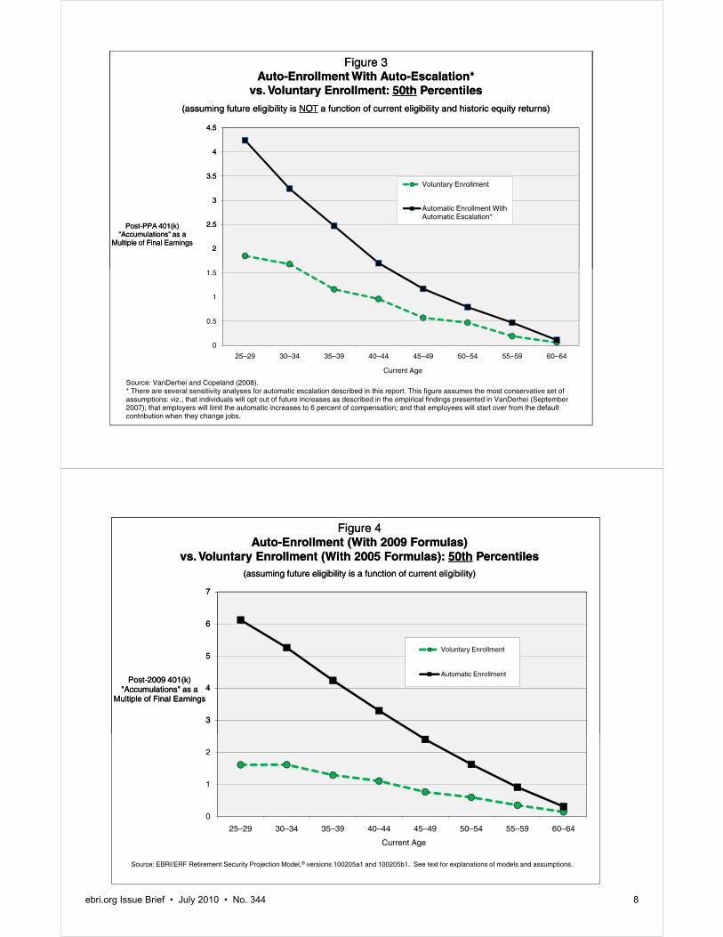
empirical evidence of whether the overall employer contribution rates to AE plans would be more or less generous than their VE counterparts. Figure 4 provides the median post-2009 401(k) accumulations as a multiple of final earnings for both VE plans (with the 2005 plan formulas) and AE plans (with the 2009 plan formulas) as a function of current age. For those currently ages 25–29, the difference in the median multiples would be approximately 4.52 times final salary in an AE plan relative to a VE plan.

Given the extremely large differences in simulated 401(k) balances (and IRA rollovers resulting from 401(k) balances), especially for younger cohorts, it is difficult to understand how a model based primarily on pre-PPA historical behaviors and trends in defined contribution plans would be able to accurately project what 401(k) and IRA balances would accumulate to in the future.

A second NRRI “at-risk” percentage is included for each age cohort in Figure 1. The original NRRI did not explicitly include health care costs; however, this was fixed in 2008 (Munnell et al., 2008), and the overall “at-risk” percentages for 2006 increased from 44 percent to 61 percent as a result. More recently (Munnell et al., March 2009), the NRRI model was modified to attempt to incorporate long-term care into the model with two alternative strategies:

Purchasing long-term care insurance.

Refraining from taking a reverse annuity mortgage, so that housing equity is potentially available to fund long-term care.

The implementation of these alternative strategies in NRRI produced very similar results, with the overall “at-risk” percentages for 2006 increasing to either 64 or 65 percent. In contrast, since its inception in 2003, RSPM has recognized that very few retirees actually have long-term care insurance and chooses to deal with this potentially catastrophic risk by stochastically generating both frequency and severity functions for each household in each of their 1,000 simulated lifepaths.16

For purposes of historical comparisons, the 2003 Retirement Readiness Ratings are also included in Figure 1. The Retirement Readiness Ratings show there has been a significant decrease in the “at-risk” levels for all three groups between 2003 and 2010, with the largest decrease (12.9 percentage points) experienced by the Gen Xers. The major reason for the large magnitude of these decreases is attributed to the projection of future defined contribution account balances (which would have the largest impact on the youngest group). As mentioned above, the 2010 Retirement Readiness Ratings fully reflect the trend to auto-enrollment, auto-escalation of contributions, and QDIAs as a result of PPA and subsequent regulations. While some plans had already adopted auto-escalation at the time of the 2003 model, the percentage of workers affected was minimal and hence not included in the simulations.

Baseline by Preretirement Income Groups

Although the 2010 Retirement Readiness Ratings show relatively little change in “at-risk” probability by age cohort, Figure 5 shows a significant impact of the relative level of preretirement income.17 In this case, households in the lowest one-third when ranked by age-specific preretirement income are simulated to be “at risk” 70.3 percent of the time, while the middle-income group has an “at-risk” percentage of 41.6 percent. This figure drops to 23.3 percent for the highest-income group.

The 2010 Retirement Readiness Ratings show a much greater variation with income group than do similar results produced by NRRI (Munnell et al., October 2009). In their model, the “at-risk” percentages vary only from 60 percent for the lowest-income group to 42 percent for the highest-income group. Again, there are several reasons to expect significant differences in the results of the two models, but one of the major differences no doubt stems from the two approaches to determine retirement wealth created by 401(k) and other defined contribution plans. RSPM provides annual micro-simulations for participation, contribution, asset allocation, and cash-out behavior, whereas as NRRI is based solely on point-in-time extrapolations of the wealth-to-income patterns by age group based on historical data from 1983–2004 (a time period prior to virtually all of the experience under auto-enrollment, auto-escalation of contributions, and the creation of QDIAs and the explosive trend in target-date funds).


Again for historical comparisons, the 2003 Retirement Readiness Ratings by income group are included in Figure 5. Both the middle- and high-income cohorts experience a 16 percentage point decrease, while the low-income cohort has a Retirement Readiness Rating that decreases by only 9 percentage points between 2003 and 2010. While this may appear counterintuitive at first given the huge positive impact of auto-enrollment and auto-escalation of contributions on the low income (VanDerhei and Copeland, 2008 and VanDerhei, 2010), the explanation will be clear later in this Issue Brief (Figure 8) when it is demonstrated how far many of the lower-income cohorts are from the point they will no longer be classified as “at risk.”

Baseline by Age Cohort and Preretirement Income Quartile

Figure 6 shows the 2003 and 2010 baseline Retirement Readiness Ratings by both age cohort and preretirement income quartile simultaneously. Similar to Figure 1, there appears to be very little, if any, trend by age cohort for most preretirement income quartiles in 2010. The one exception is for the lowest-income quartile, where the “at-risk” level is 81 percent for the Early Boomers and then drops substantially to 74 percent for the younger age cohorts. This is likely due to the impact of switching to AE 401(k) plans while the worker is young enough to benefit from the new plan design for several years prior to retirement.

Comparing the 2003 and 2010 Retirement Readiness Ratings shows at least a double-digit decrease in “at-risk” percentages for all groups except the lowest-income quartile for the Early Boomers (2 percentage point decrease) and the Late Boomers (6 percentage point decrease). Not only are many of the lowest-income quartile workers (regardless of age) often located too far from the “at-risk” threshold to have any real chance of having retirement income adequacy by retirement age, those closest to retirement age will have the least amount of time to benefit from the switch to programs that will produce a significant increase in participation rates for low-income workers.

Sensitivity Analysis on Baseline RSPM While the “at-risk” percentages in Figures 1, 5, and 6 provide a convenient summary statistic of the percentage of households that are likely to have inadequate retirement income, they provide little information on the dispersion around this binary variable.18 For example, public policy concerns may be vastly different if a significant percentage of “at-risk” households are extremely close to meeting the definition of adequacy, as opposed to those who miss the threshold by a very wide margin.

Figure 7 provides this sensitivity analysis on the baseline RSPM by age cohort, while Figure 8 provides a similar analysis by preretirement “income” quartile. In each case, the figures display the percentage of households expected to be at or above the percentage of deemed adequate income. The percentage of deemed adequate income is defined as:

For those households not at risk: 1+ (the individual account balance accumulated at the time all members of the household have died, divided by the accumulated value of the total retirement expenditures for the household); and

For those households at risk: 1– (accumulated value of deficits generated at the time all members of the household have died, divided by the accumulated value of the total retirement expenditures for the household).

Admittedly, this formulation results in an asymmetric treatment of deficits vs. surplus balances, but it provides a relatively simple way of determining what percentage of households are close to the threshold. For example, the following shows the impact of modifying the threshold for “at-risk” determination from Figure 7:

Those “At Risk,” by Income Threshold Percentage of Deemed Adequate Income Early Boomers Late Boomers Gen Xers 100% 47.2% 43.7% 44.5% 90% 35.0 32.0 34.1 80% 18.4 16.9 19.7

20%

30%

40%

50%

60%

70%

80%

90%

100%

Figure 5Impact of Income Group on At-Risk* Probability

Percentage of population “at risk” for inadequate retirement income, by age-specific remaining career income group (baseline assumptions)

Baseline�RSPM�2010


NRRI�With�2009�Corrections�for�SCF�Asset�Values

0%

10%

20%

30%

40%

50%

60%

70%

80%

90%

100%

Low Income Middle Income High Income

Figure 5Impact of Income Group on At-Risk* Probability

Percentage of population “at risk” for inadequate retirement income, by age-specific remaining career income group (baseline assumptions)



NRRI�With�2009�Corrections�for�SCF�Asset�Values

Source: EBRI Retirement Security Projection Model® versions 100504e and 100708e, and “The National Retirement Risk Index: After the Crash,” Center for Retirement Research at Boston College, October 2009. * An individual or family is considered to be “at risk” in this version of the model if their aggregate resources in retirement are not sufficient to meet aggregate minimum retirement expenditures defined as a combination of deterministic expenses from the Consumer Expenditure Survey (as a function of income) and some health insurance and out-of-pocket health related expenses, plus stochastic expenses from nursing home and home health care expenses (at least until the point they are picked up by Medicaid). The resources in retirement will consist of Social Security (either status quo or one of the specified reform alternatives), account balances from defined contribution plans, IRAs and/or cash balance plans, annuities from defined benefit plans (unless the lump-sum distribution scenario is chosen) and (in some cases) net housing equity (either in the form of an annuity or as a lump-sum distribution). This version of the model is constructed to simulate "basic" retirement income adequacy; however, alternative versions of the model allow similar analysis for replacement rates, standard of living and other ad hoc thresholds.

Income Group

Figure 6Impact of Age and Income Group on Retirement Readiness Rating

Percentage of population “at risk”* for inadequate retirement income, by age cohort

70%

80%

90%

Percentage of population at risk for inadequate retirement income, by age cohortand age-specific remaining career income groups (baseline assumptions)

2003 2010

40%

50%

60%

70%

10%

20%

30%

40%

0%

Lowest 2 3 Highest Lowest 2 3 Highest Lowest 2 3 Highest


Source: EBRI Retirement Security Projection Model® versions 100504e and 100708e.* An individual or family is considered to be “at risk” in this version of the model if their aggregate resources in retirement are not sufficient to meet aggregate minimum retirement expenditures defined as a combination of deterministic expenses from the Consumer Expenditure Survey (as a function of income) and some health insurance and out-of-pocket health-related expenses, plus stochastic expenses from nursing home and home health care expenses (at least until the point they are picked up by Medicaid) The resources in retirement will consist of Social

Age Cohort, by Income Group

and home health care expenses (at least until the point they are picked up by Medicaid). The resources in retirement will consist of Social Security (either status quo or one of the specified reform alternatives), account balances from defined contribution plans, IRAs and/or cash balance plans, annuities from defined benefit plans (unless the lump-sum distribution scenario is chosen), and (in some cases) net housing equity (either in the form of an annuity or as a lump-sum distribution). This version of the model is constructed to simulate "basic" retirement income adequacy; however, alternative versions of the model allow similar analysis for replacement rates, standard-of-living, and other ad hoc thresholds.



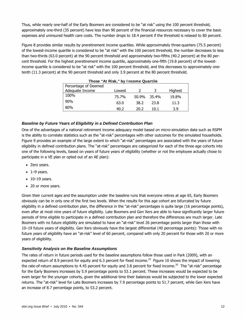
Thus, while nearly one-half of the Early Boomers are considered to be “at risk” using the 100 percent threshold, approximately one-third (35 percent) have less than 90 percent of the financial resources necessary to cover the basic expenses and uninsured health care costs. The number drops to 18.4 percent if the threshold is relaxed to 80 percent.

Figure 8 provides similar results by preretirement income quartiles. While approximately three-quarters (75.5 percent) of the lowest-income quartile is considered to be “at risk” with the 100 percent threshold, the number decreases to less than two-thirds (63.0 percent) at the 90 percent threshold and approximately two-fifths (40.2 percent) at the 80 per-cent threshold. For the highest preretirement income quartile, approximately one-fifth (19.8 percent) of the lowest-income quartile is considered to be “at risk” with the 100 percent threshold, and this decreases to approximately one-tenth (11.3 percent) at the 90 percent threshold and only 3.9 percent at the 80 percent threshold.

Those “At Risk,” by Income Quartile Percentage of Deemed Adequate Income Lowest 2 3 Highest 100% 75.7% 50.9% 35.4% 19.8% 90% 63.0 38.2 23.8 11.3 80% 40.2 20.2 10.1 3.9

Baseline by Future Years of Eligibility in a Defined Contribution Plan

One of the advantages of a national retirement income adequacy model based on micro-simulation data such as RSPM is the ability to correlate statistics such as the “at-risk” percentages with other outcomes for the simulated households. Figure 9 provides an example of the large extent to which “at-risk” percentages are associated with the years of future eligibility in defined contribution plans. The “at-risk” percentages are categorized for each of the three age cohorts into one of the following levels, based on years of future years of eligibility (whether or not the employee actually chose to participate in a VE plan or opted out of an AE plan):

Zero years.

1–9 years.

10–19 years.

20 or more years.

Given their current ages and the assumption under the baseline runs that everyone retires at age 65, Early Boomers obviously can be in only one of the first two levels. When the results for this age cohort are bifurcated by future eligibility in a defined contribution plan, the difference in the “at-risk” percentages is quite large (16 percentage points), even after at most nine years of future eligibility. Late Boomers and Gen Xers are able to have significantly larger future periods of time eligible to participate in a defined contribution plan and therefore the differences are much larger. Late Boomers with no future eligibility are simulated to have an “at-risk” level 26 percentage points larger than those with 10–19 future years of eligibility. Gen Xers obviously have the largest differential (40 percentage points): Those with no future years of eligibility have an “at-risk” level of 60 percent, compared with only 20 percent for those with 20 or more years of eligibility.

Sensitivity Analysis on the Baseline Assumptions

The rates of return in future periods used for the baseline assumptions follow those used in Park (2009), with an expected return of 8.9 percent for equity and 6.3 percent for fixed income.19 Figure 10 shows the impact of lowering the rate-of-return assumptions to 4.45 percent for equity and 3.8 percent for fixed income.20 The “at-risk” percentage for the Early Boomers increases by 5.9 percentage points to 53.1 percent. These increases would be expected to be even larger for the younger cohorts, given the additional time their balances would be subjected to the lower expected returns. The “at-risk” level for Late Boomers increases by 7.9 percentage points to 51.7 percent, while Gen Xers have an increase of 8.7 percentage points, to 53.2 percent.

20%

30%

40%

50%

60%

70%

80%

90%

Percentage of PopulationExpected to Be at Percentage of Deemed Adequate Income

or Lower

Figure 7Sensitivity Analysis on Baseline RSPM, by Age Cohort

Percentage of population "at risk"* for inadequate retirement income, by age cohort (baseline assumptions)

Early Boomers

Late Boomers

Gen Xers

0%

10%

20%

30%

40%

50%

60%

70%

80%

90%

0% 50% 100% 150% 200% 250% 300% 350%

Percentage of PopulationExpected to Be at Percentage of Deemed Adequate Income

or Lower

Percentage of Deemed Adequate Income

Figure 7Sensitivity Analysis on Baseline RSPM, by Age Cohort

Percentage of population "at risk"* for inadequate retirement income, by age cohort (baseline assumptions)

Early Boomers

Late Boomers

Gen Xers

Sources: EBRI Retirement Security Projection Model® versions 100504e and 100601e.* An individual or family is considered to be “at risk” in this version of the model if their aggregate resources in retirement are not sufficient to meet aggregate minimum retirement expenditures defined as a combination of deterministic expenses from the Consumer Expenditure Survey (as a function of income) and some health insurance and out-of-pocket health-related expenses plus stochastic expenses from nursing home and home health care expenses (at least until the point they are picked up by Medicaid). The resources in retirement will consist of Social Security (either status quo or one of the specified reform alternatives), account balances from defined contribution plans, IRAs and/or cash balance plans, annuities from defined benefit plans (unless the lump-sum distribution scenario is chosen), and (in some cases) net housing equity (either in the form of an annuity or as a lump-sum distribution). This version of the model is constructed to simulate "basic" retirement income adequacy; however, alternative versions of the model allow similar analysis for replacement rates, standard-of-living, and other ad hoc thresholds.

20%

30%

40%

50%

60%

70%

80%

90%

100%

Percentage of PopulationExpected to Be at Per-

centage of Deemed Adequate Income or Lower

Figure 8Sensitivity Analysis on Baseline RSPM, by Income Group

Percentage of population "at risk"* for inadequate retirement income, by age-specific remaining career income quartiles (baseline assumptions)

Lowest

2

3

Hi h t

Remaining Career Income Quartile

0%

10%

20%

30%

40%

50%

60%

70%

80%

90%

100%

0% 50% 100% 150% 200% 250% 300% 350% 400% 450% 500%

Percentage of PopulationExpected to Be at Per-

centage of Deemed Adequate Income or Lower

Percentage of Deemed Adequate Income

Figure 8Sensitivity Analysis on Baseline RSPM, by Income Group

Percentage of population "at risk"* for inadequate retirement income, by age-specific remaining career income quartiles (baseline assumptions)

Lowest

2

3

Highest

Sources: EBRI Retirement Security Projection Model® versions 100504e and 100601e.* An individual or family is considered to be “at risk” in this version of the model if their aggregate resources in retirement are not sufficient to meet aggregate minimum retirement expenditures defined as a combination of deterministic expenses from the Consumer Expenditure Survey (as a function of income) and some health insurance and out-of-pocket health-related expenses, plus stochastic expenses from nursing home and home health care expenses (at least until the point they are picked up by Medicaid). The resources in retirement will consist of Social Security (either status quo or one of the specified reform alternatives), account balances from defined contribution plans, IRAs and/or cash balance plans, annuities from defined benefit plans (unless the lump-sum distribution scenario is chosen), and (in some cases) net housing equity (either in the form of an annuity or as a lump-sum distribution). This version of the model is constructed to simulate "basic" retirement income adequacy; however, alternative versions of the model allow similar analysis for replacement rates, standard-of-living, and other ad hoc thresholds.

Remaining Career Income Quartile


30%

40%

50%

60%

70%

80%

90%

100%

0 1–9 10–19 20+

Figure 9Impact of Age and Future Years of Eligibility for Participation

in a Defined Contribution Plan on At-Risk* ProbabilitiesPercentage of population “at risk” for inadequate retirement income,

by age cohort, and future years eligible for participation

Future Years of Eligible Participation

0%

10%

20%

30%

40%

50%

60%

70%

80%

90%

100%


0 1–9 10–19 20+

Source: EBRI Retirement Security Projection Model® version 100504e.* An individual or family is considered to be “at risk” in this version of the model if their aggregate resources in retirement are not sufficient to meet aggregate minimum retirement expenditures defined as a combination of deterministic expenses from the Consumer Expenditure Survey (as a function of income) and some health insurance and out-of-pocket health-related expenses, plus stochastic expenses from nursing home and home health care expenses (at least until the point they are picked up by Medicaid). The resources in retirement will consist of Social Security (either status quo or one of the specified reform alternatives), account balances from defined contribution plans, IRAs and/or cash balance plans, annuities from defined benefit plans (unless the lump-sum distribution scenario is chosen), and (in some cases) net housing equity (either in the form of an annuity or as a lump-sum distribution). This version of the model is constructed to simulate "basic" retirement income adequacy; however, alternative versions of the model allow similar analysis for replacement rates, standard-of-living, and other ad hoc thresholds..

Figure 9Impact of Age and Future Years of Eligibility for Participation

in a Defined Contribution Plan on At-Risk* ProbabilitiesPercentage of population “at risk” for inadequate retirement income,

by age cohort, and future years eligible for participation

Future Years of Eligible Participation

30%

40%

50%

60%

70%

80%

90%

100%

Baseline Lower Rate of Return

Figure 10Impact of Lowering the Rate-of-Return Assumptions From 8.9% Equity and

6.3% Fixed Income to 4.45% Equity and 3.8% Fixed Income Percentage of population “at risk”* for inadequate retirement income, by age cohort

0%

10%

20%

30%

40%

50%

60%

70%

80%

90%

100%


Baseline Lower Rate of Return

Source: EBRI Retirement Security Projection Model® version 100504e vs. 100505e.* An individual or family is considered to be “at risk” in this version of the model if their aggregate resources in retirement are not sufficient to meet aggregate minimum retirement expenditures defined as a combination of deterministic expenses from the Consumer Expenditure Survey (as a function of income) and some health insurance and out-of-pocket health-related expenses, plus stochastic expenses from nursing home and home health care expenses (at least until the point they are picked up by Medicaid). The resources in retirement will consist of Social Security (either status quo or one of the specified reform alternatives), account balances from defined contribution plans, IRAs and/or cash balance plans, annuities from defined benefit plans (unless the lump-sum distribution scenario is chosen), and (in some cases) net housing equity (either in the form of an annuity or as a lump-sum distribution). This version of the model is constructed to simulate "basic" retirement income adequacy; however, alternative versions of the model allow similar analysis for replacement rates, standard-of-living, and other ad hoc thresholds.

Figure 10Impact of Lowering the Rate-of-Return Assumptions From 8.9% Equity and

6.3% Fixed Income to 4.45% Equity and 3.8% Fixed Income Percentage of population “at risk”* for inadequate retirement income, by age cohort



Policy Changes

Another advantage of the RSPM model over other models computing retirement income adequacy is that it is able to provide policy analysts with feedback on how various policy changes might be expected to modify the “at-risk” percentages of various segments of the population. Figure 11 provides analysis of a generic type of Social Security reform proposal that, in essence, would keep Social Security retirement benefits in their current statutory form until 2037 (the year in which the trust fund is estimated to reach zero under the intermediate set of assumptions in The 2009 Annual Report of the Board of Trustees of the Federal Old-Age and Survivors Insurance and Federal Disability Insurance Trust Funds), and at that point subject all Social Security retirement benefits to a permanent 24 percent reduction.21

As expected, the impact should be minimal for those currently on the verge of retirement—so the “at-risk” level for Early Boomers increases by only 0.3 percentage points. But Late Boomers will have a larger percentage of their expected Social Security benefits reduced as a result of this change, and their “at-risk” level increases by 1.6 percent-age points under the baseline assumptions. Gen Xers will have even more years of their expected retirement affected by this change, and their increase in “at-risk” percentage is simulated to be 5.8 percentage points.

Given that the Gen Xer cohort would experience a significantly larger effect under this modification, this cohort is the exclusive focus when analyzing the impact by preretirement income quartile. Since Social Security represents a larger percentage of total retirement income for retirees with lower income,22 it would be expected that the lowest-income quartile would experience a larger overall impact from the proposed Social Security benefit decrease than their higher-income counterparts.

This is borne out by the results in Figure 12. The lowest-income quartile is simulated to have an increase of 7.2 per-centage points in their “at-risk” level, compared with only 6.9 percentage points for the second quartile, 5.2 percentage points for the third quartile, and 4.2 percentage points for the highest-income quartile.

A second policy change that has been discussed recently that would affect the retirement income adequacy of current workers is a modification of Medicare benefits. One such proposal is found in the “Roadmap for America’s Future” issued by Rep. Paul Ryan (R-WI).23 While insufficient detail is available to simulate the complete proposal, this analysis attempts to approximate some of the major components by assuming Medicare beneficiaries will receive, on average, $11,000 per year, indexed for inflation by a blended rate of the Consumer Price Index (CPI) and the medical care component of the CPI. The payment amount is modified based on income: Beneficiaries with incomes below $80,000 ($160,000 for couples) receive the full standard payment amounts; beneficiaries with annual incomes between $80,000–$200,000 ($160,000–$400,000 for couples) receive 50 percent of the standard; and beneficiaries with incomes above $200,000 ($400,000 for couples) receive 30 percent.

Figure 13 shows the impact of this change on “at-risk” percentages. Similar to the Social Security modification, it has the largest impact on younger cohorts: 9.3 percentage points for Gen Xers, 2.9 percentage points for Late Boomers, and only 0.3 percentage points for Early Boomers.

Another policy change that has been suggested in previous years as an attempt to increase overall retirement income and therefore reduce the “at-risk” percentage is a mandatory individual account in addition to Social Security, which would require each employee to contribute a stipulated percentage of wages in addition to the current FICA taxation. Obviously, the net impact of such a modification would require detailed modeling on the likely substitution effect between the new mandatory add-on contribution and the possible reduction in employee savings through defined contribution or IRA contributions and/or employer modifications in retirement plan provisions. Still, a first approximation for the gross amount of new savings can be modeled at this time and used to see if the reduction in simulated “at-risk” levels is of the same magnitude as the combined impact of the increase in “at-risk” levels from reducing Social Security benefits and Medicare modifications, as mentioned above.

20%

30%

40%

50%

60%

70%

80%

90%

100%

Baseline Reduced Social Security Benefits

Figure 11Impact of Reducing Social Security Benefits by 24% Starting in 2037


0%

10%

20%

30%

40%

50%

60%

70%

80%

90%

100%


Baseline Reduced Social Security Benefits

Source: EBRI Retirement Security Projection Model® version 100504e vs. 100504e1.* An individual or family is considered to be “at risk” in this version of the model if their aggregate resources in retirement are not sufficient to meet aggregate minimum retirement expenditures defined as a combination of deterministic expenses from the Consumer Expenditure Survey (as a function of income) and some health insurance and out-of-pocket health-related expenses, plus stochastic expenses from nursing home and home health care expenses (at least until the point they are picked up by Medicaid). The resources in retirement will consist of Social Security (either status quo or one of the specified reform alternatives), account balances from defined contribution plans, IRAs and/or cash balance plans, annuities from defined benefit plans (unless the lump-sum distribution scenario is chosen), and (in some cases) net housing equity (either in the form of an annuity or as a lump-sum distribution). This version of the model is constructed to simulate "basic" retirement income adequacy; however, alternative versions of the model allow similar analysis for replacement rates, standard-of-living and other ad hoc thresholds.



30%

40%

50%

60%

70%

80%

90%

100%

Baseline

Reduced Social Security Benefits


Percentage of population “at risk”* for inadequate retirement income, by income quartile for Gen Xers only

0%

10%

20%

30%

40%

50%

60%

70%

80%

90%

100%

Lowest 2 3 HighestIncome Quartile

Baseline

Reduced Social Security Benefits

Source: EBRI Retirement Security Projection Model® version 100504e vs. 100504e1.* An individual or family is considered to be “at risk” in this version of the model if their aggregate resources in retirement are not sufficient to meet aggregate minimum retirement expenditures defined as a combination of deterministic expenses from the Consumer Expenditure Survey (as a function of income) and some health insurance and out-of-pocket health-related expenses, plus stochastic expenses from nursing home and home health care expenses (at least until the point they are picked up by Medicaid). The resources in retirement will consist of Social Security (either status quo or one of the specified reform alternatives), account balances from defined contribution plans, IRAs and/or cash balance plans, annuities from defined benefit plans (unless the lump-sum distribution scenario is chosen), and (in some cases) net housing equity (either in the form of an annuity or as a lump-sum distribution). This version of the model is constructed to simulate "basic" retirement income adequacy; however, alternative versions of the model allow similar analysis for replacement rates, standard-of-living, and other ad hoc thresholds.


Percentage of population “at risk”* for inadequate retirement income, by income quartile for Gen Xers only



Figure 14 provides the results of a contribution add-on amounting to 3 percent of compensation (assuming no impact on employee contributions or employer retirement plans). Given the additional time that Gen Xers would be contributing (assuming the new contributions begin immediately), they have the largest reduction in “at-risk” levels, at 10.4 percentage points. Smaller reductions apply to the older cohorts: 4.2 percentage points for Late Boomers and 1.5 percentage points for Early Boomers.

Figure 15 provides the results of combining all three modifications (Social Security benefit reduction, Medicare reform, and 3 percent add-on), assuming no impact on employee contributions or employer retirement plans. The additional retirement wealth generated by the additional savings more than makes up for the modification of the Social Security benefits and Medicare for the Early and Late Boomers, and their simulated “at-risk” levels decrease by 0.8 and 0.6 per-centage points, respectively. The overall impact on Gen Xers is almost completely offset by the additional savings, and their “at-risk” level increases by only 0.03 percentage points. However, there is still a significant difference in the impact of the combination of programs for Gen Xers when broken out by preretirement income quartile. Figure 16 shows that the “at-risk” level for the lowest preretirement income quartile would increase by 7.1 percentage points, while the second and third quartiles would both have less than a 0.5 percentage-point change. The highest-income quartile would have its “at-risk” level decreased by 7.3 percentage points.

Net Housing Equity The original version of RSPM in 2003 attempted to deal with the prospect of a household using net equity in the house (if any) as a means of supporting retirement expenditures by simulating whether households would be expected to have net housing equity at retirement and, if so, its expected value. Under the baseline scenario, it was assumed that retirees would not use their net housing equity to supplement their retirement income in any way (including housing equity loans). The second scenario assumed any net housing equity is annuitized at retirement. Given the stochastic nature of the analysis, a third scenario was also able to be modeled where it is assumed housing equity is not liquidated until the time it is first needed to mitigate an annual deficit. At that point it is assumed any residual value is invested in the same manner as an individual account retirement plan. Figure 17 provides the simulated “at-risk” percentages by age cohort under the baseline assumptions and the two alternatives. Under the first alternative (assuming that the households purchase a reverse annuity mortgage at age 65), the results are relatively small: Early Boomers would experience the largest reduction in the “at-risk” level of 1.8 per-centage points, decreasing to a reduction of 1.4 percentage points for Gen Xers. Similar to the results in VanDerhei and Copeland (2003), the benefit of using the net housing equity only when the household has insufficient financial resources has a larger impact (even though only approximately one-half of the households would actually sell the house under this option). In the second alternative, Early Boomers would experience the largest reduction in the “at-risk” level of 5.7 percentage points, decreasing to a reduction of 4.4 percentage points for Gen Xers.

Results for Length of Time Until the Household Runs Out of Money In addition to information with respect to the percentage of the population that will be “at-risk” of having inadequate retirement income to cover basic expenses and pay for uninsured health care costs for the remainder of their lives, the distribution of the likely number of years before those on the verge of retirement “run short of money” has been a major topic of concern.24 Figures 18 and 19 provide this type of information for the Early Boomer generation, broken down by preretirement income quartile.25 This analysis is more complicated than a simple computation of when individuals or families run short of retirement income (which in most cases will be never, due to lifetime Social Security benefits). Instead, an individual or family is considered to “run short of money” in this version of the model if their aggregate resources in retirement are not sufficient to meet aggregate minimum retirement expenditures—defined as a combination of deterministic expenses from the Consumer Expenditure Survey (as a function of income) and some health insurance and out‐of‐pocket health-related expenses, plus stochastic expenses from nursing home and home health care expenses (at least until the point they are picked up by Medicaid).

20%

30%

40%

50%

60%

70%

80%

90%

100%

Figure 13Impact of Medicare Modifications


Baseline Medicare Modifications

0%

10%

20%

30%

40%

50%

60%

70%

80%

90%

100%


Figure 13Impact of Medicare Modifications


Baseline Medicare Modifications

Sources: EBRI Retirement Security Projection Model® version 100504e vs. 100504e2; www.roadmap.republicans.budget.house.gov/plan/#Healthsecurity* An individual or family is considered to be “at risk” in this version of the model if their aggregate resources in retirement are not sufficient to meet aggregate minimum retirement expenditures defined as a combination of deterministic expenses from the Consumer Expenditure Survey (as a function of income) and some health insurance and out-of-pocket health-related expenses, plus stochastic expenses from nursing home and home health care expenses (at least until the point they are picked up by Medicaid). The resources in retirement will consist of Social Security (either status quo or one of the specified reform alternatives), account balances from defined contribution plans, IRAs and/or cash balance plans, annuities from defined benefit plans (unless the lump-sum distribution scenario is chosen), and (in some cases) net housing equity (either in the form of an annuity or as a lump-sum distribution). This version of the model is constructed to simulate "basic" retirement income adequacy; however, alternative versions of the model allow similar analysis for replacement rates, standard-of-living, and other ad hoc thresholds.

30%

40%

50%

60%

70%

80%

90%

100%

Baseline Mandatory 3% Add-on

Figure 14Impact of Mandatory 3% Add-On


0%

10%

20%

30%

40%

50%

60%

70%

80%

90%

100%


Baseline Mandatory 3% Add-on

Figure 14Impact of Mandatory 3% Add-On




30%

40%

50%

60%

70%

80%

90%

100%

Baseline

Medicare and Social Security Modifications Combined With 3% Add-On

Figure 15Impact of Medicare and Social Security Modifications

Combined With 3% Add-OnPercentage of population “at risk”* for inadequate retirement income, by age cohort

0%

10%

20%

30%

40%

50%

60%

70%

80%

90%

100%


Baseline



Combined With 3% Add-OnPercentage of population “at risk”* for inadequate retirement income, by age cohort


20%

30%

40%

50%

60%

70%

80%

90%

100%

Baseline



Combined With 3% Add-OnPercentage of population “at risk”* for inadequate retirement

income, by income quartile, Gen Xers only

0%

10%

20%

30%

40%

50%

60%

70%

80%

90%

100%

Lowest 2 3 HighestIncome Quartile

Baseline



Combined With 3% Add-OnPercentage of population “at risk”* for inadequate retirement

income, by income quartile, Gen Xers only




Figure 18 shows the distribution of how long retirement money will last for Early Boomers in each of the four preretirement income quartiles (assuming retirement at age 65). For example:

After 10 years of retirement, 41 percent of those in the lowest (preretirement) income quartile are assumed to have run short of money, but only 23 percent of the next-lowest quartile, 13 percent of the third quartile, and less than 5 percent of the highest-income quartile.

After 20 years of retirement, the numbers are 57 percent of those in the lowest-income quartile, 44 percent of the next-lowest quartile, 29 percent of the third quartile, and 13 percent of the highest-income quartile.

To illustrate, 61 percent of Early Boomers in the lowest quartile who had non-zero individual account balances at age 65 would eventually run short of money while they were still alive. This percentage drops to 49 percent for the second-lowest quartile, 35 percent for the third quartile, and only 17 percent for the highest quartile.

Figure 19 provides the same information as Figure 18, but limited only to those who run short of money in retirement. In other words, the percentages will be greater in Figure 19 than Figure 18 for any combination of income quartile and years in retirement, because these percentages are conditional upon the Early Boomer having run short of money. For example, of those Early Boomers in the lowest-income quartile who are simulated to run short of money in retirement, the median number of years before they do so is 7. This increases to 11 years for the next lowest income quartile, 13 for the third quartile, and 15 for the highest-income quartile.

Results for Percentage of Additional Compensation Needed to Eliminate Deficits Informing policymakers of the percentage of various demographic groups that are likely to be at risk for inadequate retirement income is an extremely valuable exercise.26 However, when RSPM was constructed in 2003, it was considered to be equally important to structure the simulation model so as to allow assessment of whether those at risk would be able to save additional amounts while they are still working to mitigate these risks—and, if so, how much would be needed.

This portion of the analysis combines simulated retirement income and wealth with simulated retiree expenditures to determine how much each household would need to save today (as percentage of current wages) to maintain a pre-specified “comfort level” (i.e., probability level) that they will be able to afford the simulated expenses for the remainder of the lifetime of the family unit (i.e., death of second spouse in a family).

It is important to note that within each of the groups modeled there will undoubtedly be significant percentages in the zero category27 as well as those at levels beyond which anyone could reasonably assume more than a de minimis number of individuals could possibly save. These situations are accounted for in two ways:

First, medians and 75th percentiles are reported for each of the groups. In other words, the numbers presented in Figures 20–22 provide a number representing the estimate for the 50th and 75th percentiles when ranked by percentage of compensation.

Second, the reported values of additional savings are limited to 25 percent of compensation, assuming that few (if any) households would be able to contribute in excess of this percentage on a continuous basis until retirement age.

It is also important to note that these percentages merely represent savings that need to be generated in addition to what retirement income and/or wealth is simulated by the model. Therefore, if the household is already generating savings for retirement that is not included in defined benefit or defined contribution plans, IRAs, Social Security and/or net housing equity, that value needs to be deducted from the estimated percentages.

20%

30%

40%

50%

60%

70%

80%

90%

100%

Baseline LSD** RAM**&

Figure 17Impact of Net Housing Equity Utilization


Impact of Net Housing Equity UtilizationPercentage of population “at risk”* for inadequate

retirement income, by age cohort



***

0%

10%

20%

30%

40%

50%

60%

70%

80%

90%

100%


Baseline LSD** RAM**&

Figure 17Impact of Net Housing Equity Utilization


Source: EBRI Retirement Security Projection Model® version 100504e vs. 100504e3 and 100504e4.* An individual or family is considered to be “at risk” in this version of the model if their aggregate resources in retirement are not sufficient to meet aggregate minimum retirement expenditures defined as a combination of deterministic expenses from the Consumer Expenditure Survey (as a function of income) and some health insurance and out-of-pocket health-related expenses, plus stochastic expenses from nursing home and home health care expenses (at least until the point they are picked up by Medicaid). The resources in retirement will consist of Social Security (either status quo or one of the specified reform alternatives), account balances from defined contribution plans, IRAs and/or cash balance plans, annuities from defined benefit plans (unless the lump-sum distribution scenario is chosen), and (in some cases) net housing equity (either in the form of an annuity or as a lump-sum distribution). This version of the model is constructed to simulate "basic" retirement income adequacy; however, alternative versions of the model allow similar analysis for replacement rates, standard-of-living, and other ad hoc thresholds.** This option assumes the net housing equity is used when other financial resources are exhausted and used as a lump-sum distribution (LSD).*** This option assumes the net housing equity is annuitized at the time of retirement as a reverse annuity mortgage (RAM).





***

10%

20%

30%

40%

50%

60%

70%

Cum

ulat

ive

Pro

babi

lity

Figure 18Years in Retirement Before Early Boomers Run ShorSrtOut

of Money,* by Preretirement Income Quartile

Lowest

2

3

Highest

Income Quartile

0%

10%

20%

30%

40%

50%

60%

70%

0 5 10 15 20 25 30 35 40 45

Cum

ulat

ive

Pro

babi

lity

Years in Retirement (Assuming retirement at age 65)

Figure 18Years in Retirement Before Early Boomers Run Short

of Money,* by Preretirement Income Quartile

Lowest

2

3

Highest

Source: EBRI Retirement Security Projection Model® version 100610e.* An individual or family is considered to be “at risk” in this version of the model if their aggregate resources in retirement are not sufficient to meet aggregate minimum retirement expenditures defined as a combination of deterministic expenses from the Consumer Expenditure Survey (as a function of income) and some health insurance and out-of-pocket health-related expenses, plus stochastic expenses from nursing home and home health care expenses (at least until the point they are picked up by Medicaid). The resources in retirement will consist of Social Security (either status quo or one of the specified reform alternatives), account balances from defined contribution plans, IRAs and/or cash balance plans, annuities from defined benefit plans (unless the lump-sum distribution scenario is chosen), and (in some cases) net housing equity (either in the form of an annuity or as a lump-sum distribution). This version of the model is constructed to simulate "basic" retirement income adequacy; however, alternative versions of the model allow similar analysis for replacement rates, standard-of-living, and other ad hoc thresholds.

Income Quartile


20%

30%

40%

50%

60%

70%

80%

90%

100%C

umul

ativ

e P

roba

bilit

y

Figure 19For Early Boomers Simulated to Run ShShortut of Money* in Retirement:

Distribution of the Number of Years in Retirement Before They Do So, by Preretirement Income Quartile

Lowest

2

3

Highest

Income Quartile

0%

10%

20%

30%

40%

50%

60%

70%

80%

90%

100%

0 5 10 15 20 25 30 35 40 45

Cum

ulat

ive

Pro

babi

lity

Years in Retirement (Assuming retirement at age 65)

Figure 19For Early Boomers Simulated to Run Short of Money* in Retirement:

Distribution of the Number of Years in Retirement Before They Do So, by Preretirement Income Quartile

Lowest

2

3

Highest

Source: EBRI Retirement Security Projection Model® version 100610e.* An individual or family is considered to be “at risk” in this version of the model if their aggregate resources in retirement are not sufficient to meet aggregate minimum retirement expenditures defined as a combination of deterministic expenses from the Consumer Expenditure Survey (as a function of income) and some health insurance and out-of-pocket health-related expenses, plus stochastic expenses from nursing home and home health care expenses (at least until the point they are picked up by Medicaid). The resources in retirement will consist of Social Security (either status quo or one of the specified reform alternatives), account balances from defined contribution plans, IRAs and/or cash balance plans, annuities from defined benefit plans (unless the lump-sum distribution scenario is chosen), and (in some cases) net housing equity (either in the form of an annuity or as a lump-sum distribution). This version of the model is constructed to simulate "basic" retirement income adequacy; however, alternative versions of the model allow similar analysis for replacement rates, standard-of-living, and other ad hoc thresholds.

Income Quartile

10%

15%

20%

25%

Lowest 2 3 Highest

Figure 20Amounts Needed to Be Saved for a 50% Probability of Success

Median vs. 75th percentile percentage of additional compensation that must be savedeach year until retirement age for a 50% probability of "adequate" retirement

income, by age cohort and age‐specific salary quartiles (baseline assumptions)

Salary Quartiles

0%

5%

10%

15%

20%

25%

Early Boomers, Medians

Late Boomers, Medians

Gen Xers, Medians Early Boomers, 75th pctl.

Late Boomers, 75th pctl.

Gen Xers, 75th pctl.

Lowest 2 3 Highest


Median vs. 75th percentile percentage of additional compensation that must be savedeach year until retirement age for a 50% probability of "adequate" retirement


Source: EBRI Retirement Security Projection Model® version 100504e.Note: 25% = 25% or more.

Salary Quartiles



After the retirement income and wealth is simulated for each household, 1,000 observations are simulated (from retirement age until death of the individual for single males and single females, or the second person to die for families) and the present value of the aggregated deficits is computed at retirement age. Next, the future simulated retirement income accumulated to retirement age is determined, and this information is used to determine the percentage of compensation that would need to be saved to have sufficient additional income to offset the present value of accumulated deficits. At that point, the observations are rank ordered in terms of the percentages of compensation, and the 50,th 70,th and 90th percentiles of the distribution are determined.

Figure 20 shows the median and 75th percentile percentage of compensation that must be saved each year until retirement for a 50 percent probability of retirement income adequacy, when combined with simulated retirement wealth, assuming current Social Security benefits and housing equity is never liquidated. For example, the three sets of columns on the left half of Figure 20 show that for the median household of the three age cohorts modeled in this Issue Brief, only the lowest-income quartile would need to save additional amounts (over and above those already modeled) to have a 50/50 chance of retirement income adequacy.

Unfortunately, given their proximity to retirement age, the median Early Boomer percentage for the lowest-income quartile exceeds 25 percent of compensation. This suggests that at least one-half of the households in this age/income cohort will need to find alternative solutions to the problem of securing retirement income adequacy. The problem appears to be more controllable for those in the lowest-income quartile for the younger cohorts: the median additional percentage of compensation that would need to be saved for Late Boomers in the lowest-income quartile is 12 percent, and only 6 percent for Gen Xers. The median additional percentage of compensation for the other income quartiles in each age cohort is zero.

Since the medians only provide information on the household in each cohort that is exactly in the middle of the distribution, information is also provided on the 75th percentile.28 The right half of Figure 20 shows three sets of columns for this additional information. If additional savings were to be provided at levels high enough for 3 of 4 households in each cohort to have a 50/50 chance of retirement income adequacy, the lowest-income quartiles of both the Early and Late boomers would need to save more than 25 percent of compensation per year. The lowest-income quartile for Gen Xers would require less (17 percent), but this is still an amount that would be extremely difficult for most households to save.

The second-income quartiles for the 75th percentile appear to be within range for all but the Early Boomers (23 percent for Early Boomers, but only 6 percent for Late Boomers and 2 percent for Gen Xers). The third- and fourth-income quartiles all generate values of zero at the 75th percentile, with the exception of the third quartile for Early Boomers (they would be required to contribute an additional 5 percent of compensation per year).

Given that most individuals would be unlikely to choose a situation that would provide them with adequate retirement income only 50 percent of the time, this analysis also provides results for the 70 percent and 90 percent probability levels. Figure 21 shows the additional savings required to provide retirement adequacy in 7 of 10 simulated life paths, while Figure 22 provides similar numbers for a 90 percent probability of retirement income adequacy.

Focusing on the medians (the left half of the figures), both the third- and fourth-income quartiles for all three age cohorts appear to be on track for adequate retirement income in 7 of 10 simulated retirement paths (Figure 21). However, increasing the probability of success to 9 of 10 simulated lifepaths (Figure 22) shows that only the highest-income quartiles appear to be on track, with the third-income quartiles requiring between 2 percent (for Gen Xers) and 17 percent (for Early Boomers) of compensation per year as additional savings.

Conclusion The EBRI Retirement Readiness Rating™ was developed in 2003 to provide assessment of national retirement income prospects. The 2010 update uses the most recent data and considers retirement plan changes (e.g., auto-enrollment, auto-escalation of contributions, and diversified default investments resulting from the Pension Protection Act of 2006)


as well as updates for financial market performance and employee behavior (based on a database of 24 million 401(k) participants).

The baseline 2010 Retirement Readiness Rating finds that nearly one-half (47.2 percent) of the oldest cohort (Early Baby Boomers) are simulated to be “at risk” of not having sufficient retirement resources to pay for “basic” retirement expenditures as well as uninsured health care costs. The percentage “at risk” drops for the Late Boomers (to 43.7 per-cent) but then increases slightly for Generation Xers to 44.5 percent.

Households in the lowest one-third when ranked by preretirement income are simulated to be “at risk” 70.3 percent of the time, while the middle income group has an “at-risk” level of 41.6 percent. This figure drops to 23.3 percent for the highest-income group. These numbers are generally much more optimistic than those simulated for the same groups seven years earlier: In 2003, 59.2 percent of the Early Boomers were simulated to be “at risk,” as well as 54.7 percent of the Late Boomers, and 57.4 percent of the Generation Xers. When analyzed by preretirement income in 2003, households in the lowest one-third were simulated to be “at risk” 79.5 percent of the time, 57.3 percent for the middle income group and 39.6 percent for the highest income group.

This Issue Brief provides just a brief overview of the types of analyses that are feasible under the updated version of RSPM. EBRI will produce a new set of annual Retirement Readiness Ratings in the first quarter of each year starting in 2011. Moreover, several requests have been made for additional analyses since the May 2010 EBRI policy forum where these results were initially presented, and EBRI will attempt to respond to these through a series of publications in forthcoming EBRI Notes (http://ebri.org/publications/notes/).

15%

20%

25%

Lowest 2 3 Highest


Median vs. 75th percentile percentage of additional compensation that must be savedeach year until retirement age for a 70 percent probability of "adequate" retirement


Salary Quartile

0%

5%

10%

15%

20%

25%






Lowest 2 3 Highest





Salary Quartile

15%

20%

25%

Lowest

2

3

Highest




Salary Quartile

0%

5%

10%

15%

20%

25%






Lowest

2

3

Highest





Salary Quartile



Appendix

Brief Chronology of RSPM

The original version of Retirement Security Projection Model® (RSPM) was used to analyze the future economic well-being of the retired population at the state level. The Employee Benefit Research Institute and the Milbank Memorial Fund, working with the governor of Oregon, set out to see if this situation could be addressed for Oregon. The analysis29 focused primarily on simulated retirement wealth with a comparison to ad hoc thresholds for retirement expenditures, but the results made it clear that major decisions lie ahead if the state’s population is to have adequate resources in retirement.

Subsequent to the release of the Oregon study, it was decided that the approach could be carried to other states as well. Kansas and Massachusetts were chosen as the next states for analysis. Results of the Kansas study were presented to the state’s Long-Term Care Services Task Force on July 11, 2002,30 and the results of the Massachusetts study were presented on Dec. 1, 2002.31 With the assistance of the Kansas Insurance Department, EBRI was able to create Retirement Readiness Ratings based on a full stochastic decumulation model that took into account the household’s longevity risk, post-retirement investment risk, and exposure to potentially catastrophic nursing home and home health care risks. This was followed by the expansion of RSPM, as well as the Retirement Readiness Ratings produced by it, to a national model and the presentation of the first micro-simulation retirement income adequacy model built in part from administrative 401(k) data at the EBRI December 2003 policy forum.32 The basic model was then modified for Senate Aging testimony in 2004 to quantify the beneficial impact of a mandatory contribution of 5 percent of compensation.33

The first major modification of the model occurred for the EBRI May 2004 policy forum. In an analysis to determine the impact of annuitizing defined contribution and IRA balances at retirement age, VanDerhei and Copeland (2004) were able to demonstrate that for a household seeking a 75 percent probability of retirement income adequacy, the additional savings that would otherwise need to be set aside each year until retirement to achieve this objective would decrease by a median amount of 30 percent. Additional refinements were introduced in 2005 to evaluate the impact of purchasing long-term care insurance on retirement income adequacy.34

The model was next used in March of 2006 to evaluate the impact of defined benefit freezes on participants by simulating the minimum employer contribution rate that would be needed to financially indemnify the employees for the reduction in their expected retirement income under various rate-of-return assumptions.35 Later that year, an updated version of the model was developed to enhance the EBRI interactive Ballpark E$timate® worksheet by providing Monte Carlo simulations of the necessary replacement rates needed for specific probabilities of retirement income adequacy under alternative risk management treatments.36

RSPM was significantly enhanced for the May 2008 EBRI policy forum by allowing automatic enrollment of 401(k) participants with the potential for automatic escalation of contributions to be included.37 Additional modifications were added in 2009 for a Pension Research Council presentation that involved a winners/losers analysis of defined benefit freezes and the enhanced defined contribution employer contributions provided as a quid pro quo.38

A new subroutine was added to the model to allow simulations of various styles of target-date funds for a comparison with participant-directed investments in 2009.39 Most recently, the model was completely reparameterized with 401(k) plan design parameters for sponsors that have adopted automatic enrollment provisions.40

Retirement Income and Wealth Assumptions

RSPM is based in part on a 13-year time series of administrative data from several million 401(k) participants and tens of thousands of 401(k) plans,41 as well as a time series of several hundred plan descriptions used to provide a sample of the various defined benefit and defined contribution plan provisions applicable to plan participants. In addition, several public surveys based on participants’ self-reported answers (the Survey of Consumer Finances [SCF], the Current Population Survey [CPS], and the Survey of Income and Program Participation [SIPP]) were used to model participation, wages, and initial account balance information.


This information is combined to model participation and initial account balance information for all defined contribution participants, as well as contribution behavior for non-401(k) defined contribution plans. Asset allocation information is based on previously published results of the EBRI/ICI Participant-Directed Retirement Plan Data Collection Project, and employee contribution behavior to 401(k) plans is provided by an expansion of a method developed in VanDerhei and Copeland (2008) and further refined in VanDerhei (2010).

A combination of Form 5500 data and self-reported results was also used to estimate defined benefit participation models; however, it appears information in the latter is rather unreliable with respect to estimating current and/or future accrued benefits. Therefore, a database of defined benefit plan provisions for salary-related plans was constructed to estimate benefit accruals.

Combinations of self-reported results were used to initialize IRA accounts. Future IRA contributions were modeled from SIPP data, while future rollover activity was assumed to flow from future separation from employment in those cases in which the employee was participating in a defined contribution plan sponsored by the previous employer. Industry data are used to estimate the relative likelihood that the balances are rolled over to an IRA, left with the previous employer, transferred to a new employer, or used for other purposes.

Defined Benefit Plans

A stochastic job duration algorithm was estimated and applied to each individual in RSPM to predict the number of jobs held and age at each job change. Each time the individual starts a new job, RSPM simulates whether or not it will result in coverage in a defined benefit plan, a defined contribution plan, both, or neither. If coverage in a defined benefit plan is predicted, time series information from the Bureau of Labor Statistics (BLS) is used to predict what type of plan it will be.42

While the BLS information provides significant detail on the generosity parameters for defined benefit plans, preliminary analysis indicated that several of these provisions were likely to be highly correlated (especially for integrated plans). Therefore, a time series of several hundred defined benefit plans per year was coded to allow for assignment to the individuals in RSPM.43

Although the Tax Reform Act of 1986 at least partially modified the constraints on integrated pension plans by adding Sec. 401(l) to the Internal Revenue Code, it would appear that a significant percentage of defined benefit sponsors have retained Primary Insurance Amount (PIA)-offset plans. In order to estimate the offset provided under the plan formulas, RSPM computes the employee’s Average Indexed Monthly Earnings, Primary Insurance Amount, and covered compensation values for the birth cohort.

Defined Contribution Plans

Previous studies on the EBRI/ICI Participant-Directed Retirement Plan Data Collection Project have analyzed the average account balances for 401(k) participants by age and tenure. Recently published results (VanDerhei, Holden and Alonso, 2009) show that the year-end 2008 average balance ranged from $3,237 for participants in their 20s with less than three years of tenure with their current employer to $172,555 for participants in their 60s who have been with the current employer for at least 30 years (thereby effectively eliminating any capability for IRA rollovers).

Unfortunately, the EBRI/ICI database does not currently provide detailed information on other types of defined contribution plans nor does it allow analysis of defined contribution balances that may have been left with previous employers. RSPM uses self-reported responses for whether an individual has a defined contribution balance to estimate a participation model and the reported value is modeled as a function of age and tenure.

The procedure for modeling participation and contribution behavior and asset allocation for defined contribution plans that have not adopted automatic enrollment is described in VanDerhei and Copeland (2008). The procedure for modeling contribution behavior (with and without automatic escalation of contributions) for 401(k) plans is described in VanDerhei (2010). Asset allocation for automatic enrollment plans is assumed to follow average age-appropriate target-date funds as described in VanDerhei (2009). Investment returns are based on those used in Park (2009).


Social Security Benefits

Social Security’s current-law benefits are assumed to be paid and received by those qualifying for the benefits under the baseline scenario. This funding could either be from an increase in the payroll tax or from a general revenue transfer. The benefits are projected for each cohort assuming the intermediate assumptions within the 2009 OASDI Trustee’s Report. A second alternative is used where all recipients’ benefits are cut 24 percent on the date that the OASDI Trust Fund is depleted (2037).

Expenditure Assumptions

The expenditures used in the model for the elderly consist of two components—deterministic and stochastic expenses. The deterministic expenses include those expenses that the elderly incur in their basic daily life, while the stochastic expenses in this model are exclusively health-event related—such as an admission to a nursing home or the commencement of an episode of home health care—that occur only for a portion, if ever, during retirement, not on an annual or certain basis.

Deterministic Expenses

The deterministic expenses are broken down into seven categories—food, apparel and services (dry cleaning, haircuts), transportation, entertainment, reading and education, housing, and basic health expenditures. Each of these expenses is estimated for the elderly (65 or older) by family size (single or couple) and family income (less than $20,000, $20,000–$39,999, and $40,000 or more in 2008 dollars) of the family/individual.

The estimates are derived from the 2008 Consumer Expenditure Survey (CES) conducted by the Bureau of Labor Statistics of the U.S. Department of Labor. The survey targets the total noninstitutionalized population (urban and rural) of the United States and is the basic source of data for revising the items and weights in the market basket of consumer purchases to be priced for the Consumer Price Index. Therefore, an expense value is calculated using actual experience of the elderly for each family size and income level by averaging the observed expenses for the elderly within each category meeting the above criteria. The basic health expenditure category has additional data needs besides just the CES.

Health

The basic health expenditures are estimated using a somewhat different technique and are comprised of two parts. The first part uses the CES as above to estimate the elderly’s annual health expenditures that are paid out-of-pocket or are not fully reimbursed (or not covered) by Medicare and/or private Medigap health insurance.

The second part contains insurance premium estimates, including Medicare Part B and Part D premiums. All of the elderly are assumed to participate in Part B and Part D, and the premium is determined annually by the Medicare program and is the same nationally with an increasing contribution from the individual/family on the basis of their income. For the Medigap insurance premium, it is assumed all of the elderly purchase a Medigap policy. A national estimate is derived from a 2005 survey done by Thestreet.com that received average quotes for Plan F in 47 states and the District. The estimates are calculated based on a 65-year-old female. The 2005 premium level is the average of the 47 state average quotes. The 2010 premium level was estimated by applying the annual growth rates in the Part B premiums from 2006 through 2010 to the average 2005 premium.

This approach is taken for two reasons. First, sufficient quality data do not exist for the matching of retiree medical care (as well as the generosity of and cost of the coverage) and Medigap policy use to various characteristics of the elderly. Second, the health status of the elderly at the age of 65 is not known, let alone over the entire course of their remaining life. Thus, by assuming everyone one has a standard level of coverage eliminates trying to differentiate among all possible coverage types as well as determining whether the sick or healthy have the coverage. Therefore, averaging of the expenses over the entire population should have offsetting effects in the aggregate.

The total deterministic expenses for the elderly individual or family are then the sum of the values in all the expense categories for family size and family income level of the individual or family. These expenses make up the basic annual


(recurring) expenses for the individual or family. However, if the individual or family meet the income and asset tests for Medicaid, Medicaid is assumed to cover the basic health care expenses (both parts), not the individual or family. Furthermore, Part D and Part B premium relief for the low-income elderly (not qualifying for Medicaid) is also incorporated.

Stochastic Expenses

The second component of health expenditures is the result of simulated health events that would require long-term care in a nursing home or home-based setting for the elderly. Neither of these simulated types of care would be reimbursed by Medicare because they would be for custodial (not rehabilitative) care. The incidence of the nursing home and home health care and the resulting expenditures on the care are estimated from the 1999 and 2004 National Nursing Home Survey (NNHS) and the 2000 and 2007 National Home and Hospice Care Survey (NHHCS). NNHS is a nationwide sample survey of nursing homes, their current residents and discharges that was conducted by the National Center for Health Statistics from July through December 1999 and 2004. The NHHCS is a nationwide sample survey of home health and hospice care agencies, their current and discharge patients that was conducted by the National Center for Health Statistics from August 2000 through December 2000 and from August 2007 through February 2008.

For determining whether an individual has these expenses, the following process is undertaken. An individual reaching the Social Security normal retirement age has a probability of being in one of four possible assumed “health” statuses:

Not receiving either home health or nursing home care,

Home health care patient,

Nursing home care patient,

Death,

based upon the estimates of the use of each type of care from the surveys above and mortality. The individual is randomly assigned to each of these four categories with the likelihood of falling into one of the four categories based upon the estimated probabilities of each event. If the individual does not need long-term care, no stochastic expenses are incurred. Each year, the individual will again face these probabilities (the probabilities of being in the different statuses will change as the individual becomes older after reaching age 75 then again at age 85) of being in each of the four statuses. This continues until death or the need for long-term care.

For those who have a resulting status of home health care or nursing home care, their duration of care is simulated based upon the distribution of the durations of care found in the NNHS and NHHCS. After the duration of care for a nursing home stay or episode of home health care, the individual will have a probability of being discharged to one of the other three statuses based upon the discharge estimates from NNHS and NHHCS, respectively. The stochastic expenses incurred are then determined by the length of the stay/number of days of care times the per diem charge estimated for the nursing home care and home health care, respectively.

For any person without the need for long-term care, this process repeats annually. The process repeats for individuals receiving home health care or nursing home care at the end of their duration of stay/care and subsequently if not receiving the specialized care again at their next birthday. Those who are simulated to die, of course, are not further simulated.

As with the basic health care expenses, the qualification of Medicaid by income and asset levels is considered to see how much of the stochastic expenses must be covered by the individual to determine the individual’s final expenditures for the care. Only those expenditures attributable to the individualnot the Medicaid programare considered as expenses to the individual and as a result in any of the “deficit” calculations.


Total Expenditures

The elderly individuals’ or families’ expenses are then the sum of their assumed deterministic expenses based upon their retirement income plus any simulated stochastic expenses that they may have incurred. In each subsequent year of life, the total expenditures are again calculated in this manner. The base year’s expenditure value estimates excluding the health care expenses are adjusting annually using the assumed general inflation rate of 2.8 percent from the 2009 OASDI Trustees Report, while the health care expenses are adjusted annually using the 4.0 percent medical consumer price index that corresponds to the average annual level from 20042009.44


References Copeland, Craig, and Jack VanDerhei. The Declining Role of Private Defined Benefit Pension Plans: Who Is Affected,

and How. Oxford University Press, “Restructuring Retirement Risk Management in a Defined Contribution World,” (forthcoming).

Holden, Sarah, and Jack VanDerhei. “The Influence of Automatic Enrollment, Catch-Up, and IRA Contributions on 401(k) Accumulations at Retirement.” EBRI Issue Brief, no. 283 (Employee Benefits Research Institute, July 2005).

Ippolito, Richard A. Pension Plans and Employee Performance: Evidence, Analysis, and Policy. Chicago: University of Chicago, 1997.

McDonnell, Ken. “Income of the Elderly Population Age 65 and Over, 2008.” EBRI Notes, no. 6 (June 2010): 2–7.

Munnell, Alicia H., Anthony Webb, and Francesca Golub-Sass. “The National Retirement Risk Index: After The Crash.” Issue In Brief, 9–22. Chestnut Hill, MA: Center for Retirement Research at Boston College, October 2009.

Munnell, Alicia H., Mauricio Soto, Anthony Webb, Francesca Golub-Sass, and Dan Muldoon. “Health Care Costs Drive up the National Retirement Risk Index.” Issue in Brief, 8–3. Chestnut Hill, MA: Center for Retirement Research at Boston College, February 2008.

Munnell, Alicia H., Anthony Webb, Francesca Golub-Sass, and Dan Muldoon. “Long-Term Care Costs and the National Retirement Risk Index.” Issue In Brief, 9−7. Chestnut Hill, MA: Center for Retirement Research at Boston College, March 2009.

Park, Youngkyun. “Plan Demographics, Participants’ Saving Behavior, and Target-Date Fund Investments.” EBRI Issue Brief, no. 329 (Employee Benefit Research Institute, May 2009).

Ryan, Paul D. A Roadmap for America’s Future, Version 2.0, A Plan to Solve America’s Long-Term Economic and Fiscal Crisis. Committee on the Budget, January 2010.

VanDerhei, Jack. Testimony for the U.S. Senate Special Committee on Aging Hearing on Retirement Planning: “Do We Have a Crisis in America? Results From the EBRI-ERF Retirement Security Projection Model,” Jan. 27, 2004 (T-141).

_____. “Measuring Retirement Income Adequacy, Part One: Traditional Replacement Ratios and Results for Workers at Large Companies.” EBRI Notes, no. 9 (Employee Benefit Research Institute, September 2004): 2−12.

_____. Projections of Future Retirement Income Security: Impact of Long- Term Care Insurance, American Society on Aging/National Council on Aging joint conference, March 2005.

_____. “Defined Benefit Plan Freezes: Who's Affected, How Much, and Replacing Lost Accruals.” EBRI Issue Brief, no. 291 (Employee Benefit Research Institute, March 2006).

_____. "Measuring Retirement Income Adequacy: Calculating Realistic Income Replacement Rates." EBRI Issue Brief, no. 297 (Employee Benefit Research Institute, September 2006).

_____. “Retirement Income Adequacy After PPA and FAS 158: Part One─Plan Sponsors' Reactions.” EBRI Issue Brief, no. 307 (Employee Benefit Research Institute, July 2007).

_____. “The Expected Impact of Automatic Escalation of 401(k) Contributions on Retirement Income.” EBRI Notes, no. 9 (Employee Benefit Research Institute, September 2007): 1−8.

_____. How Would Target-Date Funds Likely Impact Future 401(k) Contributions. Testimony before the joint DOL/SEC Hearing, Target Date Fund Public Hearing, June 2009.


_____. “The Impact of Automatic Enrollment in 401(k) Plans on Future Retirement Accumulations: A Simulation Study Based on Plan Design Modifications of Large Plan Sponsors.” EBRI Issue Brief, no. 341 (Employee Benefit Research Institute, April 2010).

VanDerhei, Jack, and Craig Copeland. Oregon Future Retirement Income Assessment Project. A project of the EBRI Education and Research Fund and the Milbank Memorial Fund, 2001.

_____. Kansas Future Retirement Income Assessment Project. A project of the EBRI Education and Research Fund and the Milbank Memorial Fund, July 16, 2002.

_____. Massachusetts Future Retirement Income Assessment Project. A project of the EBRI Education and Research Fund and the Milbank Memorial Fund, December 1, 2002.

_____. “Can America Afford Tomorrow's Retirees: Results From the EBRI-ERF Retirement Security Projection Model.” EBRI Issue Brief, no. 263 (Employee Benefit Research Institute, November 2003).

_____. “ERISA At 30: The Decline of Private-Sector Defined Benefit Promises and Annuity Payments: What Will It Mean?” EBRI Issue Brief, no. 269 (Employee Benefit Research Institute, May 2004).

_____. ”The Impact of PPA on Retirement Income for 401(k) Participants.” EBRI Issue Brief, no. 318 (Employee Benefit Research Institute, June 2008).

VanDerhei, Jack, Sarah Holden, and Louis Alonso. “401(k) Plan Asset Allocation, Account Balances, and Loan Activity in 2008.” EBRI Issue Brief, no. 335, and ICI Perspective, Vol. 15, no. 2 (Employee Benefit Research Institute and Investment Company Institute, October 2009).


Endnotes 1 See VanDerhei (September 2004) for a description of the various approaches to benchmarking retirement income needs. 2 For a description of the EBRI/ICI Participant-Directed Retirement Plan Data Collection Project, see the October 2009 EBRI Issue Brief and ICI Perspective, at www.ebri.org/publications/ib and www.ici.org/research/perspective 3 Sensitivity analysis in this Issue Brief is limited exclusively to the impact of alternative (lower) rates of return and the utilization of net housing equity on the “at risk” calculations. Additional sensitivity analysis will be published in forthcoming EBRI Notes publications. 4 The nominal cost of these expenditures increases with component-specific inflation assumptions. See the appendix for more details. 5 Net housing equity is introduced into the model in three different mechanisms (explained below). 6 IRS tax tables from 2009 are used to compute the tax owed on the amounts received from defined benefit plans and Social Security (with the percentage of Social Security benefits subject to Federal Income Tax proxied as a function of the various retirement income components) as well as the individual account withdrawals. 7 Roth IRA and 401(k) accounts are not used in this version of the model but will be incorporated into a forthcoming EBRI publication. 8 Capital gains treatment is not used in this version of the model. 9 This allows simulations for those currently ages 36–62 in 2010. In previous work with this model (VanDerhei and Copeland, 2003), workers between the ages of 38 and 67 in 2003 were simulated. 10 The nominal cost of these expenditures increase with component-specific inflation assumptions. See the appendix for more details. 11 The NRRI projects replacement rates for each member of the SCF sample of households and compares the projection with a target replacement rate that would allow the household to “maintain its preretirement standard of living in retirement.” Households whose projected replacement rates fall more than 10 percent below the target are denoted as being “at risk” of having insufficient income to meet this standard. 12 One likely difference deals with the asset allocation of investments in defined contribution plans. VanDerhei (June 2009) conducts simulations using RSPM showing the improvement in terms of risk and return for large cohorts of 401(k) participants when TDF asset allocations (simulations are run for average, conservative, and aggressive TDF asset allocations) are substituted for participant-directed investments. In contrast, the NRRI methodology is based on historical data over a time period that largely excludes any potential beneficial impact from this trend. Another difference that remains to be quantified is the assessment of defined benefit accruals. Whereas NRRI is based on SCF data that have the survey respondents assess what their eventual defined benefit payouts will be, RSPM bases the defined benefit accruals on a time series of defined benefit plan type and generosity parameters coded from, inter alia, summary plan description-type information on more than 1,000 large salaried defined benefit plans per year. 13 Munnell, Webb, and Golub-Sass (2009). 14 Until empirical information is available to track individual employees from one job to the next and track their 401(k) eligibility status, one needs to rely on some type of assumption with respect to this variable. Since there appears to be a well-documented body of evidence (Ippolito, 1997) that individuals with a propensity to save would seek out 401(k) sponsors (or vice versa), an admittedly ad-hoc approach was developed to compute eligibility probabilities conditional upon the eligibility status on the previous job, as shown below:

Let z = unconditional probability of being covered (empirical value as a function of age and wage).

Let x = probability of being covered given that your last job was covered.

Let y = probability of being covered given that your last job was NOT covered.

There are two cases for x in VanDerhei and Copeland (2008):

Complete independence (e.g., x=z=y).

An ad-hoc assumption that the value of x will be half-way between the unconditional value and 100 percent. In other words, x = (1+z)/2 and y = (z-.5*(z)(1+z))/(1-z).

There is no way to tell at this point which of these assumptions is likely to be more realistic. However, all simulations were conducted using both sets of assumptions to check the sensitivity of the results.


15 See VanDerhei (July 2007) for detail on the EBRI/Mercer survey of defined benefit sponsors to gauge their recent activity as well as planned modifications with respect to both defined benefit and defined contribution plan design. 16 EBRI has modeled the likely cost/benefit impact of purchasing long-term care insurance on retirement income adequacy. VanDerhei (2005) demonstrated that this purchase appears to be quite favorable for those in the second and third income quartile who desire more than a 50 percent chance of adequacy, whereas those in the lowest-income quartile often have the ability to satisfy the financial thresholds necessary to be covered by Medicaid and those in the fourth quartile will sometimes find self-insurance a more efficient method of dealing with this risk. 17 Preretirement income in RSPM is determined in a manner similar to the average indexed monthly earnings computation for Social Security with the following modifications:

All earned income is included up to the age of retirement (i.e., there is no maximum taxable wage base constraint and the calculation terminates at retirement age).

Instead of indexing for changes in average national wages, the model indexes based on assumed after‐tax rate of return based on asset allocations that are a function of the individual’s age in each year.

Percentile distributions are then established based on population statistics for each five‐year age cohort. Whereas households are split into three income groups in Figure 5 to allow a direct comparison with the NRRI results, the remainder of this Issue Brief presents these results as quartiles to provide more useful results.

18 We thank Stephen Goss for suggesting this improvement. 19 The standard deviations were 18.0 percent for U.S. equity, 19.1 percent for non-U.S. equity and 2.9 percent for fixed income. 20 The standard deviations were 9.0 percent for U.S. equity, 9.55 percent for non-U.S. equity and 1.75 percent for fixed income. See Park (2009) for the rationale behind these assumptions. 21 More complex Social Security reform scenarios were modeled in the original RSPM EBRI Issue Brief (VanDerhei and Copeland, 2003). These will be updated and published in a forthcoming EBRI Notes article. 22 In 2008, the lowest-income quintile among the elderly received 88.4 percent of its income from Social Security, while the highest-income quintile received 18.6 percent of its income from Social Security (McDonnell, 2010). 23 www.roadmap.republicans.budget.house.gov/

24 We are unable to compare our results with those of NRRI in this case since they assume that all individual accounts are annuitized at retirement age. In reality, only an extremely small percentage of those currently retiring appear to be annuitizing a significant percentage of their individual accounts. For example, see the public comments to “Lifetime Income Options For Participants And Beneficiaries In Retirement Plans—RFI,” at www.dol.gov/ebsa/regs/cmt-1210-AB33.html

25 In a slight departure from the previous analysis, this analysis excludes any individuals or families with zero individual account balances at age 65. This new definition has only minimal impact on the numbers produced for the figures but is computationally more efficient. This does prevent direct comparison of results from Figures 18 and 19 with those described earlier in the Issue Brief, however. 26 Charts 12–17 of the authors’ presentation at the May 13, 2010, EBRI policy forum provided additional analysis of the amounts needed to be saved for a 50, 70, and 90 percent probability of retirement income adequacy, as a function of the percentage of future years of eligibility for participation in a defined contribution plan. The charts are available at www.ebri.org/pdf/programs/policyforums/VanDerhei-Copeland0510PF.pdf 27 This does not mean they have already saved enough for retirement income adequacy at the specified level. Instead, it means that their current resources PLUS the additional retirement wealth that will be accumulated under the expected benefits from employee savings, employer-provided benefits, Social Security, and (in some cases) net housing equity would be sufficient. 28 For example, if there were 100 households in a specific cohort and their additional percentages of compensation required for retirement income adequacy were ranked in ascending order, the 75th percentile would be the percentage associated with the 75th household. In other words, only 25 percent of the households in the cohort would have percentages greater than this amount. 29 VanDerhei and Copeland (2001). 30 VanDerhei and Copeland (July 2002). 31 VanDerhei and Copeland (December 2002).


32 VanDerhei and Copeland (2003) 33 VanDerhei (January 2004). 34 VanDerhei (2005). 35 VanDerhei (March 2006). 36 VanDerhei (September 2006) 37 VanDerhei and Copeland (2008). 38 Copeland and VanDerhei (forthcoming). 39 VanDerhei (2009). 40 VanDerhei (2010). 41 The EBRI/ICI Participant-Directed Retirement Plan Data Collection Project is the largest, most representative repository of information about individual 401(k) plan participant accounts. As of December 31, 2008, the database included statistical information about:

24.0 million 401(k) plan participants, in

54,765 employer-sponsored 401(k) plans, holding

$1.092 trillion in assets.

The 2008 database covered 48 percent of the universe of active 401(k) plan participants, 12 percent of plans, and 47 percent of 401(k) plan assets. The EBRI/ICI project is unique because it includes data provided by a wide variety of plan recordkeepers and, therefore, portrays the activity of participants in 401(k) plans of varying sizes—from very large corporations to small businesses—with a variety of investment options. 42 The model is currently programmed to allow the employee to participate in a nonintegrated career average plan; an integrated career average plan; a five-year final average plan without integration; a three-year final average plan without integration; a five-year final average plan with covered compensation as the integration level; a three-year final average plan with covered compensation as the integration level; a five-year final average plan with a PIA offset; a three-year final average plan with a PIA offset; a cash balance plan, or a flat benefit plan. 43 BLS information was utilized to code the distribution of generosity parameters for flat benefit plans. 44 While the medical consumer price index only accounts for the increases in prices of the health care services, it does not account for the changes in the number and/or intensity of services obtained. Thus, with increased longevity, the rate of health care expenditure growth will be significantly higher than the 4.0 percent medical inflation rate, as has been the case in recent years.

EBRI Employee Benefit Research Institute Issue Brief (ISSN 0887137X) is published monthly by the Employee Benefit Research Institute, 1100 13th St. NW, Suite 878, Washington, DC, 20005-4051, at $300 per year or is included as part of a membership subscription. Periodi-cals postage rate paid in Washington, DC, and additional mailing offices. POSTMASTER: Send address changes to: EBRI Issue Brief, 1100 13th St. NW, Suite 878, Washington, DC, 20005-4051. Copyright 2010 by Employee Benefit Research Institute. All rights reserved. No. 344.

The Employee Benefit Research Institute (EBRI) was founded in 1978. Its mission is to contribute to, to encourage, and to enhance the development of sound employee benefit programs and sound public policy through objective research and education. EBRI is the only private, nonprofit, nonpartisan, Washington, DC-based organization committed exclusively to public policy research and education on economic security and employee benefit issues. EBRI’s membership includes a cross-section of pension funds; businesses; trade associations; labor unions; health care providers and insurers; government organizations; and service firms.

EBRI’s work advances knowledge and understanding of employee benefits and their importance to the nation’s economy among policymakers, the news media, and the public. It does this by conducting and publishing policy research, analysis, and special reports on employee benefits issues; holding educational briefings for EBRI members, congressional and federal agency staff, and the news media; and sponsoring public opinion surveys on employee benefit issues. EBRI’s Education and Research Fund (EBRI-ERF) performs the charitable, educational, and scientific functions of the Institute. EBRI-ERF is a tax-exempt organization supported by contributions and grants.

EBRI Issue Briefs are periodicals providing expert evaluations of employee benefit issues and trends, as well as critical analyses of employee benefit policies and proposals. EBRI Notes is a monthly periodical providing current information on a variety of employee benefit topics. EBRI’s Pension Investment Report provides detailed financial information on the universe of defined benefit, defined contribution, and 401(k) plans. EBRI Fundamentals of Employee Benefit Programs offers a straightforward, basic explanation of employee benefit programs in the private and public sectors. The EBRI Databook on Employee Benefits is a statistical reference work on employee benefit programs and work force-related issues. www.ebri.org

Contact EBRI Publications, (202) 659-0670; fax publication orders to (202) 775-6312. Subscriptions to EBRI Issue Briefs are included as part of EBRI membership, or as part of a $199 annual subscription to EBRI Notes and EBRI Issue Briefs. Individual copies are available with prepayment for $25 each (for printed copies). Change of Address: EBRI, 1100 13th St. NW, Suite 878, Washington, DC, 20005-4051, (202) 659-0670; fax number, (202) 775-6312; e-mail: [email protected] Membership Information: Inquiries regarding EBRI membership and/or contributions to EBRI-ERF should be directed to EBRI President/ASEC Chairman Dallas Salisbury at the above address, (202) 659-0670; e-mail: [email protected]

Editorial Board: Dallas L. Salisbury, publisher; Stephen Blakely, editor. Any views expressed in this publication and those of the authors should not be ascribed to the officers, trustees, members, or other sponsors of the Employee Benefit Research Institute, the EBRI Education and Research Fund, or their staffs. Nothing herein is to be construed as an attempt to aid or hinder the adoption of any pending legislation, regulation, or interpretative rule, or as legal, accounting, actuarial, or other such professional advice. EBRI Issue Brief is registered in the U.S. Patent and Trademark Office. ISSN: 0887137X/90 0887137X/90 $ .50+.50

© 2010, Employee Benefit Research InstituteEducation and Research Fund. All rights reserved.

Who we are

What we do

Our publications

Orders/ Subscriptions

The EBRI Retirement Readiness Rating:™ Retirement · PDF Issue Brief • July 2010...

Documents

Transcript of The EBRI Retirement Readiness Rating:™ Retirement · PDF Issue Brief • July 2010...