The effect of Medicaid on Children’s Health: a Regression

Discontinuity Approach

Dolores de la Mata∗†

Job Market Paper

This version: December 2010

Abstract

In this paper I estimate the impact of Medicaid on children’s health care utilization and their

subsequent health outcomes. I estimate the causal effects using a Regression Discontinuity (RD)

design. I exploit the discontinuity generated by Medicaid’s eligibility rule, based on family income,

on program participation rates. In contrast with a standard regression discontinuity approach,

here there are multiple eligibility thresholds that vary across states. This allows me to estimate

heterogeneous effects of the program at different income thresholds. Using data from the Panel

Study of Income Dynamics (PSID) and its Child Development Study (CDS) supplement, I find that

the effects of Medicaid on measures of children’s health are heterogeneous depending on the family

income level. Negative impacts of Medicaid are generally observed for children of higher-income

families −185 and 250% of the poverty line−, while generally null or positive effects are observed for

poorer children −with family income lower than 185% of the poverty line. A possible explanation

for the heterogeneous impacts is the differential effect of Medicaid on health care utilization. While

I find that Medicaid increases the use of preventive medical care among children with low family

income, no significant effects are observed among those with higher income. Also, if higher-income

families are switching from a private health insurance that allowed them to access to better quality

of health care than the public program, then Medicaid may have negative effects on children’s health

outcomes.

JEL Classification: I18, G22.

Keywords: Health insurance, children health, Medicaid, regression discontinuity design.

∗Department of Economics, Universidad Carlos III de Madrid. Email: mlmata@eco.uc3m.es.†I am grateful to Matilde Machado for her constant support, encouragement and valuable advice. I also want to

thank Lucila Berniell, Julio Caceres, Joaquın Coleff, Ramiro de Elejalde, Roger Feldman, Eva Garcıa Moran, FelixLobo, and participants at the UC3M Student Workshop and the UC3M Applied Economics and Econometricsseminar for helpful comments and discussions. All remaining errors are my own.

1

1 Introduction

There is strong evidence showing the positive relationship between parental socioeconomic status

and children’s health, leading to health inequalities in early childhood. To the extent that poor

health affects the formation of human capital, it is then possible that health could play a key

role in the intergenerational transmission of socioeconomic inequalities (Currie (2009), Almond

and Currie (2010)). Currie (2009) suggests that children’s health inequalities may be partially

explained by disparities in the access to health care services. The provision of public health

insurance coverage to children of low-income families facilitates the access to medical care and,

therefore, may help to break the link between socioeconomic status and health.

In this paper, I address the question of whether a public health insurance targeting poor

children contributes to the improvement of their subsequent health outcomes. In particular, I

study the contemporaneous and mid-term impacts of Medicaid, the US public health insurance

program for low-income families, on children’s health care utilization and health outcomes.

I exploit the particular characteristics of Medicaid’s eligibility rules to identify the causal

effects of the program on children’s outcomes. A child is eligible to receive Medicaid coverage

if her family income is below a given threshold, defined as a percentage of the poverty line.

This rule generates a discontinuity in the enrollment rates of children with family income close

to the threshold, which allows me to implement a regression discontinuity (RD) design. Since

enrollment into Medicaid is not mandatory, the RD design is denoted as “fuzzy” RD.

Eligibility criteria for the Medicaid program are set at the state level. Thus, the income

threshold that determines eligibility varies across states. Moreover, the income thresholds may

depend on the child’s age. The multiplicity of thresholds is advantageous for the external validity

of the RD design I implement since the effects estimated are not restricted to the individuals

located around a single income threshold, but they are averages of the effects across different

thresholds. I quantify the effects of the program on children with different levels of family

income, and check whether these effects are heterogeneous.

I use data from the Panel Study of Income Dynamics (PSID) and complement it with the

Child Development Study (CDS) supplement, which provides rich information about children’s

health and health care utilization as well as detailed information on socioeconomic characteristics

of the family. The PSID data allows tracking of children’s Medicaid status at different ages

through childhood.

2

Some studies have addressed the question of whether health insurance has a positive effect

on children’s health. Among the studies using data on Medicaid the results are mixed. For

example, Currie and Gruber (1996) find evidence that the expansions in Medicaid eligibility

thresholds between 1984 and 1992 increased the utilization of medical care and reduced child

mortality. In contrast, Currie et al. (2008) find that expansions in Medicaid eligibility thresholds

from 1986 to 2005 had no effect on the health of children between 9 and 17 years old, as reported

by their parents. Their estimates, however, suggest that expansions that affected children of

ages between 2 and 4 are associated with better health by the time they are 9-17 years old.

This paper contributes to this literature in several ways. First, I analyze both the con-

temporaneous and the lagged effects of Medicaid on different measures of health. Since health

is a stock, the effects of insurance coverage may be visible with a lag. The paper by Currie

et al. (2008) is among the first to attempt estimating these lagged effects. However, in the cross

sectional datasets they use, they must impute the family income and the state of residence of

the child, since these variables are not observed during childhood. In contrast, I exploit the

panel dimension of PSID data to match past eligibility with current health outcomes. Second,

the identification strategy I propose allows the estimation of Medicaid effects that vary across

different levels of income. Results show the importance of this disaggregation when drawing any

conclusions about the effects of the program.

Results show that Medicaid enrollment rates are relatively low, consistent with previous

findings (e.g. Currie and Gruber (1996)), and that they decrease with family income. Making

a child eligible for Medicaid increases the likelihood that she will be enrolled in the program by

12 percentage points on average.

Moreover, I find that Medicaid eligibility increases the utilization of preventive medical care

−measured by the probability of visiting a doctor for a routine check-up in the last 12 months−,

by 12 percentage points, but only for children whose family income is lower than 185% of the

poverty line. The effect is much larger for “compliers” −those who enroll in the program when it

is available. According to LATE estimates, Medicaid increases compliers’ likelihood of visiting

a doctor by 63 percentage points. I do not observe significant effects on utilization for children

with family income between 185 and 250% of the poverty line.

In the short run, Medicaid’s effects on health are null or even negative. Even the medium run

effects −1 to 3 years after being eligible− tend to be negative on average. When disaggregating

3

the results by income, however, I find that the average negative impact of Medicaid on children’s

outcomes is driven by its negative impact on the health of children in higher-income families. I

show that the impact of Medicaid on the health of poorer children is relatively higher, and in

some cases also positive.

One possible explanation for the heterogeneous effects of Medicaid on children with different

levels of family income could be the heterogeneous impact of Medicaid on health care utilization.

In fact, my findings indicate that only poorer children increase health care utilization, which in

turn may positively affect their health in the mid-run.

A second reason why Medicaid’s impact varies by family income is that while Medicaid may

be the only option for poorest families to access health care, this may not be so for higher-income

families, who, more likely, have enough resources to buy health insurance in the private market.

Then, for poorer children enrolled in Medicaid, we may expect better health outcomes because

for them the counterfactual situation is, more likely, being uninsured. However, for children of

higher-income families enrolled in Medicaid, this is not necessarily the expected effect. These

children were enrolled into Medicaid because the public insurance program allows their families

to reduce the expenditures on health care.1 But switching to the public system may have a cost

in terms of the quality of care they have access to. The higher the family income, the better

the quality of care they may be sacrificing when switching to Medicaid. In an independent and

simultaneous work, Koch (2010) also finds evidence that supports this hypothesis. His results

indicate that families with larger incomes have access to better insurance quality and that the

quality of care received by children decreases as they become eligible for public health insurance.

Hence, Medicaid coverage in this case may actually have a negative impact on children’s health.

The remainder of the paper is organized as follows: Section 2 describes the Medicaid program;

Section 3 presents the empirical strategy; Section 4 describes the data; Section 5 validates

the regression discontinuity strategy; Section 6 presents the results; and section 7 presents a

discussion of the results and concludes.

1There is a large literature studying to what extent Medicaid expansions have lead eligible families to switchfrom the private to the public sector. This effect is known in the literature as “crowding-out” effect (Cutler andGruber (1996), Lo Sasso and Buchmueller (2004), Card and Shore-Sheppard (2004), Ham and Shore-Sheppard(2005), Gruber and Simon (2007)).

4

2 Medicaid Program

The Medicaid program was introduced in the late 1960s as a health insurance component for

state cash welfare programs targeting low-income single female head families. It is a state

administered program and each state sets its own guidelines regarding eligibility and services,

but subject to federal rules requiring minimum levels of coverage and services.

Medicaid eligibility for children was in its origins tied to the participation in the Aid for

Families with Dependent Children (AFDC) program. Since the mid 1980s the linkage between

AFDC coverage and eligibility for Medicaid has been gradually weakened, by eliminating the

family structure requirements for young children and by allowing states to increase the income

thresholds that determine eligibility. The increase in the thresholds was first a state option,

but later minimum levels of coverage were imposed by federal mandates. By April 1990, states

were required to offer coverage to all children under 6 years old in families with income up to

133% of the poverty line and, starting in July 1991, they were required to provide coverage to

all children under age 19, who were born after September 1983 and lived in households with

incomes below 100% of the poverty line. As a result, by the mid-1990s, most children in the US

living in households with incomes below 100% of the poverty line, and all young children living

in households with incomes below 133% of the poverty line were eligible for Medicaid.

In practice, most states opted to raise the income thresholds beyond 133% of the poverty

level and some did further increases using own state funds. States also set different threshold

levels for different age groups. In 1997, the Medicaid program for children was augmented

by the Children’s Health Insurance Program (CHIP), which provided extra funds to expand

eligibility for children beyond the existing limits of Medicaid program. The CHIP program

was implemented either by expanding the Medicaid program, or designing a new program, with

features that mimic private health insurance.

The types of services that Medicaid must cover according to the federal rules include major

services as outpatient and inpatient hospital services. Services such as prescription drugs or

dental care are not mandatory, however all states in practice cover most of them. For the

traditional Medicaid population these services are provided with little or no copayment required

(Gruber and Simon, 2007).2 In terms of the package of services covered, Medicaid tends to be

more generous than many private insurance plans.

2In states that have CHIP, the copayments are allowed to be higher for those above 150% of the poverty line.

5

States also determine the rules to reimburse health care providers. In most cases, Medi-

caid’s reimbursement is lower than the obtained from private insurance, which may induce some

physicians to reject Medicaid patients or to lower the quality of the service provided.3

3 Identification

3.1 Contemporaneous effects

The main objective is to estimate a simple model of the causal effect of Medicaid coverage on

children’s health care utilization and health outcomes:

yi = α+ βMi + ui (1)

where Mi indicates whether the child received Medicaid coverage. A simple OLS regression

of equation 1 would yield a biased estimate. Medicaid coverage is an endogenous variable, be-

cause the access to this type of coverage is correlated with family income. Even after controlling

for family income, there exists the problem of selection, because taking Medicaid is not manda-

tory. Among eligibles, the decision to take Medicaid may be correlated with other unobserved

characteristics that are correlated with the outcomes of interest.

In order to identify the effect of interest, I exploit the rule of assignment into Medicaid to

implement a Regression Discontinuity (RD) design. The RD design is a quasi-experimental

design with the defining characteristic that the probability of receiving treatment changes dis-

continuously as a function of the variable that determines eligibility (Hahn et al. (2001)).4

The intuition behind the RD is the following. Under the assumption that families have

imperfect control of their income −which in the RD jargon is called the assignment or forcing

variable− the variation in eligibility status will be as good as randomization in the neighbor-

hood of the threshold, approximating a randomized experiment. This implies that children’s

3For example, Decker (2007) finds that higher Medicaid fees increase the number of private physicians, espe-cially in medical and surgical specialties, who see Medicaid patients. She also finds that higher fees also lead tovisit times with physicians that are more comparable to visit times with private pay patients. Another paper byCunningham and OMalley (2009) finds that not only reimbursement fees matters, but also delays in reimburse-ment. They find evidence that Medicaid reimbursement time affects physicians’ willingness to accept Medicaidpatients.

4For a comprehensive discussion of the RD design and its application in economics see Imbens and Lemieux(2008), van der Klaauw (2002), and (Lee and Lemieux, 2010)

6

observable and unobservable characteristics should have the same distribution just above and

just below the threshold. Making the additional assumption that the outcome is a smooth func-

tion of income, the causal effect of being assigned into treatment −being eligible for Medicaid−

can be identified by comparing the average outcome of children just below the income thresh-

old (“treatment group”) with children just above it (“control group”). Any difference observed

between these two groups can be attributed to the availability of treatment −being eligible to

Medicaid− for treatment group members. This difference would identify an average treatment

effect only in the case of perfect compliance, that is, the probability of receiving the treatment

−being enrolled into Medicaid− is equal one for eligible individuals and zero for non-eligibles.5

Under imperfect compliance, which is the case in my dataset because enrolling into Medicaid

is not mandatory, the comparison of outcomes of eligible and non eligible individuals close to

the threshold does not identify the average treatment effect, but the average effect of assignment

into treatment or the intent to treat effect (ITT) at the threshold.6 The ITT effects, however,

could be significantly lower in absolute value than the effect the program for those who are

actually covered by Medicaid. I can still estimate β implementing a “fuzzy” RD design under the

assumptions that the probability of treatment− having Medicaid coverage− is discontinuous at

the threshold, the association between the outcome variable and income is smooth, and persons

close to the threshold are similar in baseline (pre-treatment) characteristics.

As shown by Hahn et al. (2001), the treatment effect can be recovered by dividing the

“jump” in the relationship between the outcome and eligibility −the ITT at the threshold− by

the fraction of individuals induced to take Medicaid at the threshold:

β =limz→z−0

E[yi|zi = z]− limz→z+0E[yi|zi = z]

limz→z−0E[Mi|zi = z]− limz→z+

0E[Mi|zi = z]

(2)

where zi is the family income and z0 is the eligibility threshold.

Hahn et al. (2001) were the first to show the connection between how the treatment effect

is defined in the fuzzy RD design and the “Wald” estimation of the treatment effect in an

instrumental variables setting. They suggest estimating the treatment effect in the fuzzy RD

5This would mean that Mi is equal to and indicator of eligibility status, Elii, that takes the value one whenthe child is eligible for Medicaid.

6For instance, studies like Currie and Gruber (1996) and Currie et al. (2008), although using different identi-fication strategies than in this paper, identify the intent to treat effects of Medicaid on children who where newlyeligible to receive Medicaid benefits with the Medicaid expansion.

7

setting using two-stage least-squares (TSLS). Furthermore, they also pointed out that equation

2 can be interpreted as a Local Average Treatment Effect (LATE) at the threshold under the

same assumptions as in Imbens and Angrist (1994). Under these assumptions, the LATE is

defined as the average effect of treatment on eligible individuals at the threshold who receive the

treatment if and only if they are assigned to it. These individuals are called the “compliers”.

Given that Medicaid is a state administered program, and that each state sets its own

eligibility threshold, there are multiple thresholds. Assuming that treatment effects are different

for different thresholds, the estimates obtained using a sample that pools all states reflects an

average of LATE’s at each threshold.

I implement a parametric RD strategy that controls for a flexible function of income as pro-

posed by van der Klaauw (2002), in order to retain observations that are not necessarily close to

threshold. This flexible function of income controls for variation coming from income differences

far from the threshold. I also include flexible functions of other variables that determine eligi-

bility (family size, and child age) and I follow a similar functional specification as in Carneiro

and Ginja (2009).

First I estimate the following equation:

yi = α+ θElii + fg(zit; γg) + ui (3)

where Elii is a dummy variable that takes the value one if the child is eligible for Medicaid,

fg(zit; γg) is a flexible function of income −second-order polynomials in my baseline estimations−

and other determinants of eligibility. The parameter θ is the ITT effect of Medicaid. The periods

for which I observe the outcomes are t=1997, 2002, 2007, as I explain in section 4.

I also implement the Fuzzy RD parametrically −using polynomial regression− and estimate

β by 2SLS, where I instrument the treatment dummy Mi with Eligibility, Elii. The two equation

system is:

yi = α+ βMi + k2g(zi;α2g) + ui (4)

Mi = π0 + π1Elii + k1g(zi;α1g) + vi (5)

8

where k1g(.) and k1g(.) are polynomials of order g of zi (family income, child’s age and family

size), and ui and vi are an unobserved error components. Since the model is exactly identified,

2SLS estimates or β are numerically identical to the ratio of the reduced form coefficients θ/π1,

provided the same order of polynomial is used for k1(.) and k2(.) (Lee and Lemieux, 2010). In

all the baseline estimates I use second order polynomials.

3.2 Lagged effects

In order to identify mid-run effects of Medicaid, I should account for the possibility of mul-

titreatment. Children may have multiple opportunities to be assigned to treatment during

their childhood. Therefore, the dynamic dimensions of the effects of the Medicaid Program are

twofold: 1) the effects of being assigned to treatment or receiving treatment in a given period

t may be visible −in terms of health outcomes− with some lag, 2) current assignment to treat-

ment may affect participation in the program in subsequent periods, which in turn may have a

cumulative effect on health.

Then, the marginal effect of making a child randomly eligible for Medicaid in a period t− τ

on health outcomes in period t would reflect a cumulative effect which is the sum of: 1) a direct

effect on health outcomes τ years later, if it were possible to prohibit her from being assigned

to treatment in any other subsequent period; 2) an indirect effect on health outcomes through

the effects on subsequent participation in the program. The total effect or mid-run ITT effect

Medicaid eligibility on subsequent health is the effect of exogenously making a child eligible in a

given period, without controlling for the family behavior in subsequent years. Following Cellini

et al. (2010) the ITT parameter is:7

θITTτ =dyit

dElii,t−τ=

∂yit∂Mi,t−τ

× ∂Mi,t−τ∂Elii,t−τ

+

τ∑h=1

(∂yit

∂Mi,t−τ+h×∂Mi,t−τ+h

∂Elii,t−τ

)(6)

where Elii,t−τ is a dummy variable that takes the value one if the child was eligible for

Medicaid in the year t − τ ; ∂yit∂Mi,t−τ

is the direct effect of Medicaid in period t − τ under the

assumption that the child would not have access to Medicaid in the subsequent years.8

7The main difference with Cellini et al. (2010) is that in their paper they have a “sharp” RD design, that is,being eligible is equivalent to receiving the treatment.

8Health outcomes in period t can be written as a function of the history of eligibility status yit =∑Tτ=0 δτElii,t−τ + ui. Each of the partial effects δτ capture the direct effects of Medicaid eligibility on sub-

9

I implement an RD design similar Cellini et al. (2010) to estimate the θITTτ parameters. I

regress the outcomes in period t on eligibility status t − τ , controlling for flexible functions of

family income and family characteristics in t − τ but not for any subsequent income or other

characteristics:

yit = α+ θτElii,t−τ + fg(zi,t−τ ; γτ ) + uit (7)

where fg is a polynomial of order g. As in previous specifications the baseline estimate

controls for second-order polynomials of income and other variables that determine eligibility,

such as age and family size.

4 Data

I use the data from the Child Development Study (CDS), a supplementary study to the Panel

Study of Income Dynamics (PSID). The CDS gathers information of a nationally representative

sample of children between 1 and 12 years old by 1997 and collects health care utilization and

health outcomes, obtained from the child’s primary caregiver, as well as characteristics such as

age and race of the child. Data for this cohort of children were collected in three waves: 1997,

2002, and 2007. Information on family income, Medicaid coverage, and family characteristics is

provided in the PSID dataset. I use the three CDS waves-matched with PSID data as repeated

cross-sections, and I restrict the sample to children between 5 and 18 years old. I keep only

those children for whom I can follow back their eligibility and Medicaid status up to 5 years

before the outcomes are observed.

First, I assign Medicaid eligibility status of each child in the survey on a yearly basis. To

impute eligibility I need to compare the annual family income with the annualized income

threshold that determines eligibility. The family income is reported in each wave of PSID and

it always refers to the previous calendar year. I compute the income threshold that corresponds

to each child, zoit, according to the following formula:

zoit = PLt(family sizeit)× kt(stateit, ageit) (8)

sequent outcomes. Cellini et al. (2010) propose a methodology to estimate also these partial effects.

10

where PLt is the poverty threshold in period t and kt(.) is the state-age specific factor of

adjustment in period t. I use the annualized official poverty threshold which is provided in

the PSID data file for each family.9 I get the information of state-age-year specific adjustment

factors from various reports of the National Governors’ Association. All income measures are

expressed in 2000 dollars. A child is eligible for Medicaid in period t if his family income is

below the income threshold, Eliit = 1{incomeit <= zoit}.

I use three types of outcome variables: preventive health care utilization, objective measures

of health, and subjective measures of health. The measure of preventive health care utilization

is a variable that indicates whether the child had visited a doctor at least once in the last 12

months for a routine health check-up. This measure is generally used to capture the utilization

of medical resources for preventive purposes. Other measures of health care utilization, such as

the number of hospitalizations, may confound access and morbidity, as pointed out by Currie

and Gruber (1996). An absence of a doctor visits for a regular check-up, however, better reflects

an “access” problem. Preventive medical care may help to improve and maintain the health

stock of the child, hence it is an important measure to look at.

For an objective measure of the child health I use the Body Mass Index (BMI).10 A child’s

weight status is determined based on an age and sex-specific percentile for BMI rather than

by the BMI categories used for adults, because children’s body composition varies as they age

and varies between boys and girls. The CDS dataset provides indicators of the child’s obesity

and overweight status, based on the Centers for Disease Control and Prevention (CDC) growth

charts.11 Hence, a child is classified as obese if her BMI is at or above the 95th percentile of

the BMI distribution of children of the same age and sex. A child is overweight if her BMI is

at or above the 85th percentile but below the 95th percentile. Medicaid coverage may facilitate

and increase the contact with physicians, which in turn increases the likelihood that children’s

weight status is monitored. Physicians recommendations about the quality of the diet and the

adequate level of physical activity the child might do, may be critical inputs to improve poorer

children’s health status.

Additionally, I use two subjective health measures, both reported by the child’s caregiver:

9See Grieger et al. (2009) for further details on the measures of family income and poverty thresholds in PSID.10Although it is not completely “objective”, since during the interview, the primary caregiver reports the weight

of the child, and the interviewer measures his or her height11Each of the CDC BMI-for-age gender specific charts contains a series of curved lines indicating specific

percentiles. See the CDC Growth Charts for children at: http:\www.cdc.gov\growthcharts.

11

an indicator of whether the child has an excellent health status and a dummy of whether the

child missed more than five days of school due to illness during the last 12 months. The first

measure reflects the caregiver’s perception about the child’s overall health status. I interpret

any deviation from excellent health as reflecting some health problem. The second measure links

child’s health status and school attendance, thus, it captures some aspect of how health may

affect her human capital formation. A better health status allows to prevent illnesses and to be

in better health for not missing school days.

One drawback of using subjective health measures is that they are difficult to interpret.

Currie and Gruber (1996) argue that these measures may capture two possible effects. If the

public insurance coverage leads individuals to increase the contacts with the medical system,

then there could be a “true” effect on child health, resulting in better child’s health reports.

The increased contacts with physicians, however, may also affect parents’ perception about the

health of the child. Parents may learn about health conditions the child already had but, because

they did not contact physicians so frequently before having the public insurance coverage, they

were not aware of them. Also, if targeted children are switching from a private insurance to the

public, parent’s reports may be sensitive to perceived changes in the quality of health care they

have access with the public insurance relative to the private. Thus, these measures should be

interpreted with caution.

Samples I restrict the sample to children for whom I observe all the outcomes of interest

in at least one of the three CDS waves. I pool the three years treating them as repeated cross

sections.12 Each outcome is matched with eligibility and Medicaid status up to 5 years before

the outcomes is observed.

The objective is to analyze the effect of making someone randomly eligible in a given year,

on his outcomes τ years latter. I look at effects up to 5 years later, thus τ takes values from 0

to 5. I center the periods in the year t when outcomes are observed (t = 1997, 2002, 2007). To

estimate both the contemporaneous effect and each of the lagged effects of Medicaid −which I

do in separate regressions− I define a specific sample according to the following criteria. In each

sample, I keep those children whose family income in the period t− τ was close to the eligibility

threshold of that period. Because of the small sample sizes I would get by restricting the analysis

only to observations in a tight neighborhood of the threshold, I focus on an implementation of the

12All estimations control for year effects.

12

RD strategy that retains observations that may be far from it. The parametric RD estimation

I implement uses a flexible function of income to absorb the variation coming from non-close

income levels. The baseline estimates are based on samples of individuals whose family income,

in the respective year eligibility is analyzed, is within a distance of ± 50 thousand dollars from

the income threshold.

The means describing the main characteristics of the sample are presented in the table 1.13

Columns 1 and 2 present descriptive statistics for the full sample. Columns 3 to 8 present

the same descriptives but for three subsamples, defined by the level of Medicaid generosity in

each state: the first subsample is composed of children living in states where the generosity

of Medicaid coverage is relatively low −the eligibility thresholds are less than 185% of the

poverty line; the second subsample keeps children living in states with middle level of generosity

−the eligibility thresholds are between 185 and 250% of the poverty line; and finally, the third

subsample is composed by children living in states with relatively high levels of generosity −the

eligibility thresholds are above 250% of the poverty line.

From columns 1 and 2, it is clear that Medicaid eligibles are more disadvantaged than

non-eligibles in several dimensions. They have not only lower family income −by definition of

eligible− but also they are likely to be minorities, to live in a female-headed family, and to

live with a less educated head of household. They are worse off in terms of health outcomes;

however they are more likely to have visited a doctor for a check up in the last 12 months.

The same picture emerges if I split the sample according to the different levels of Medicaid’s

coverage generosity. In the 3 groups, eligible children are always more disadvantaged in terms

of socioeconomic characteristics, they also tend to have worse health outcomes and to use more

preventative health are services, with the exception of states with higher levels of Medicaid

generosity, where utilization is higher for non-eligibles.

About 53% of eligible children are actually enrolled in Medicaid, although enrollment is

heterogeneous depending on family income level.14 The incentives to enroll in Medicaid decreases

13These descriptive statistics corresponds to the sample selected to analyze the contemporaneous effects ofMedicaid. That is, it is restricted to children whose annual family income is within a distance of ± 50 thousanddollars in period t, for t=1997, 2002, and 2007.

14Notice that among non-eligibles there are individuals with Medicaid coverage. This happens because theremay be timing problems in the reports of individuals eligibility and Medicaid coverage. Also, income fluctuationsduring the year can make an individual eligible for Medicaid but using their annual income I classify them asnon-eligible. Approximately 10% of the non-eligibles in the full sample report having Medicaid, although thispercentage rise up to a 20% for the subgroup of individuals just below the eligibility threshold, as will be showedin section 5.

13

with income, as can be observed by comparing eligible children in states with increasing levels of

Medicaid generosity. The take-up rate is 61% in states with modest Medicaid coverage generosity,

where eligibles’ average family income is 12.1 thousand dollars per year; this proportion falls to

53% in states with middle level generosity and where eligibles’ average income is 21.4 thousand

dollars; and it is even lower −35%− in states with the most generous coverage, where eligibles’

average income is 33,6 thousand dollars. The incentives to enroll in Medicaid may decline with

income because, as income rises, the family’s financial constraint is less binding, which allows

them to acquire an alternative source of coverage in private markets.

14

Table 1: Descriptive Statistics

Pooling all Thresholds Thresholds<185 Thresholds [185,250] Thresholds>250Eligible Non-Eligible Eligible Non-Eligible Eligible Non-Eligible Eligible Non-Eligible

(1) (2) (3) (4) (5) (6) (7) (8)

Outcome Measures

Visited a doctor at least once in last 12 months 0.75 0.68 0.70 0.62 0.76 0.71 0.74 0.77

Obese (over 95 percentile BMI dist.) 0.24 0.19 0.23 0.19 0.24 0.20 0.28 0.17

Overweight (85-95 percentile BMI dist.) 0.15 0.15 0.15 0.15 0.15 0.16 0.14 0.18

Obese + Overweight 0.39 0.35 0.38 0.34 0.39 0.36 0.42 0.35

More than 5 days of school missed 0.12 0.12 0.18 0.12 0.10 0.13 0.12 0.11

Health Excellent 0.39 0.54 0.27 0.47 0.42 0.58 0.47 0.62

Insurance Coverage

Medicaid Coverage 0.53 0.09 0.61 0.12 0.53 0.07 0.35 0.05

Private Insurance 0.32 0.81 0.21 0.77 0.32 0.82 0.58 0.90

Family and Child Characteristics

Family Income (2000 dollars) 20,438 53,349 12,101 44,120 21,352 58,124 33,641 78,361(12,481) (18,574) (7,325) (15,010) (11,076) (16,290) (15,220) (20,573)

Income Cutoff (eligibility threshold) 35,768 30,898 22,465 21,315 37,260 35,681 56,647 58,971(13,557) (12,832) (6,755) (5,993) (9,339) (8,384) (13,475) (14,546)

Income threshold as % of poverty line 200.65 174.30 123.68 120.02 205.67 201.91 341.23 331.43(66.33) (61.07) (24.56) (24.62) (18.05) (16.45) (46.78) (41.84)

Metropolitan Area 0.67 0.60 0.76 0.60 0.64 0.57 0.61 0.80

Rural Area 0.15 0.16 0.11 0.14 0.15 0.20 0.20 0.090.35 0.37 0.31 0.35 0.36 0.40 0.40 0.28

Family Size 4.20 4.09 4.30 4.09 4.24 4.08 3.75 4.08(1.35) (1.13) (1.34) (1.07) (1.38) (1.19) (1.16) (1.16)

Education (yrs.) of the Head of the Household 11.84 12.92 11.91 12.66 11.69 12.97 12.55 14.10(2.29) (2.04) (1.84) (2.01) (2.47) (2.00) (1.98) (2.13)

Female Head 0.61 0.23 0.68 0.27 0.60 0.21 0.46 0.16

Child Age 11.20 10.97 9.41 9.57 11.82 12.09 11.74 12.30(3.17) (3.28) (3.18) (2.96) (2.93) (3.05) (2.95) (3.26)

Male 0.52 0.50 0.49 0.50 0.52 0.51 0.58 0.52

Black 0.61 0.35 0.73 0.45 0.61 0.29 0.37 0.30

Hispanic 0.06 0.03 0.00 0.01 0.09 0.04 0.00 0.00

Birth Weight (kg) 3.20 3.36 3.17 3.34 3.19 3.37 3.30 3.38(0.69) (0.64) (0.72) (0.65) (0.67) (0.64) (0.71) (0.60)

Mother Age at Child’s Birth 25.16 27.02 25.22 26.61 25.06 27.21 25.63 27.94(6.01) (5.37) (5.97) (5.14) (6.12) (5.55) (5.49) (5.29)

N 1,127 1,668 284 700 713 835 130 105

Observations are always restricted to children whose family income is at a distance of ± 50 thousand dollars from the threshold in years 1997, 2002 or 2007.

15

5 Validity of RD design: robustness analysis

The empirical strategy is based on the assumption that eligibility to receive Medicaid coverage

is as good as randomly assigned in the neighborhood of the income thresholds. This implies

that individuals at either side of the threshold are similar both in observed and unobserved

characteristics. Additionally, for the validity of the design, it should be observed a jump in

the probability of participation at the threshold, and no signs of manipulation of the forcing

variable. A first step in the analysis, therefore, involves testing these identification assumptions.

To check the validity of the design I perform a series of robustness analyses, as proposed by

Imbens and Lemieux (2008) and Lee and Lemieux (2010). First, I inspect the histogram of the

family income −the assignment variable− to check whether individuals have imprecise control

over it. A spike to the left of the threshold may indicate that families may be manipulating their

income to fall below the eligibility threshold. Second, I estimate the enrollment equation to check

whether the eligibility rule induces a discontinuity in Medicaid participation at the threshold.

Finally, I examine whether baseline covariates (variables that should not be affected by the

program as well as individual characteristics not taken into account to participate) are balanced

on either side of the threshold. I run falsification tests to check whether the discontinuity in

eligibility status affects these variables.

5.1 Manipulation of the assignment variable

Figure 1 presents the distribution of family income, pooling all observations for the period 1994

to 2007. Given that there are multiple thresholds, income is normalized by subtracting the

corresponding eligibility threshold. A negative difference indicates that the child is eligible for

Medicaid. I calculate the number of observations within bins of 2.5 thousand dollars width.

An accumulation of observations below the normalized threshold (equal to zero) may be an

indication of income manipulation. At first sight it does not seem that families manipulate their

income in order to be below the threshold.

16

Figure 1: Distribution of the Family Income. Years 1994-2007.

17

5.2 Discontinuity in the probability of participating in Medicaid

As I discussed in section 3, an RD analysis can still identify treatment effects despite imperfect

compliance, as long as the eligibility rule generates a jump in the participation rate at the

threshold. I check this assumption first with a graphical analysis and them by a regression

analysis.

Figure 2 plots the proportion of children who are enrolled in Medicaid over family income.

This proportion is calculated within family income bins of 2 thousand dollars width. We can

observe that at the threshold −which in this graph is normalized to 0− the probability of

participation has a discontinuity of about 10 percentage points.

Figure 2: Participation decision

Table 2 reports the results of the parametric estimate of the participation equation specified

as:

Mi,t−τ = π0 + π1Elii,t−τ + k1g(zi,t−τ ;α1g) + ui,t−τ (9)

where Elii,t−τ is the eligibility indicator in period t − τ and Mi,t−τ is Medicaid enrollment

status in the same period, for τ = 0, ..., 5. Each row of table 2 reports the participation equation

for different subsamples, according to the period in which eligibility is analyzed. The first

column reports the estimated jump in the probability of participation at the threshold, for a

sample that pools all states, that is, all possible thresholds. Making a child with family income

at the threshold eligible for Medicaid increases the probability of enrollment between about 12

18

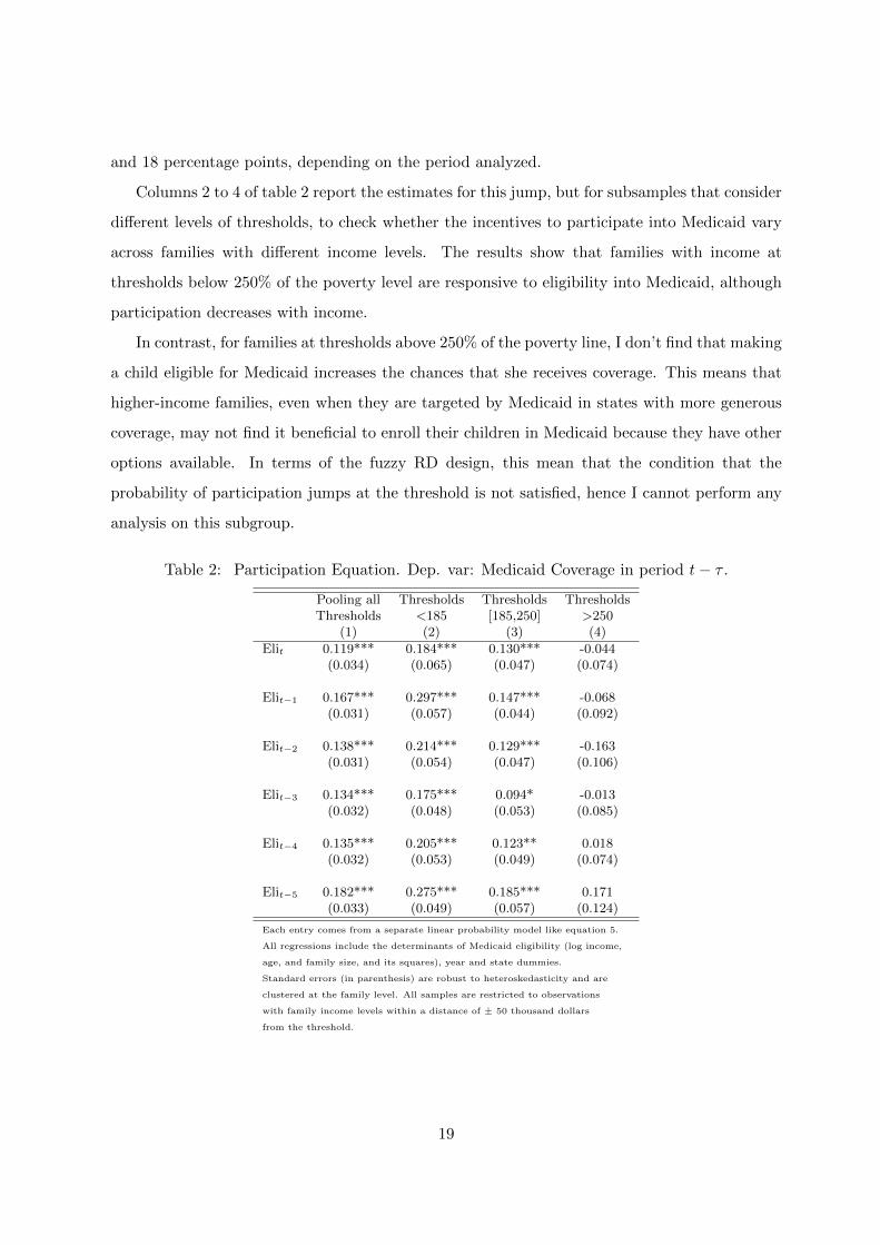
and 18 percentage points, depending on the period analyzed.

Columns 2 to 4 of table 2 report the estimates for this jump, but for subsamples that consider

different levels of thresholds, to check whether the incentives to participate into Medicaid vary

across families with different income levels. The results show that families with income at

thresholds below 250% of the poverty level are responsive to eligibility into Medicaid, although

participation decreases with income.

In contrast, for families at thresholds above 250% of the poverty line, I don’t find that making

a child eligible for Medicaid increases the chances that she receives coverage. This means that

higher-income families, even when they are targeted by Medicaid in states with more generous

coverage, may not find it beneficial to enroll their children in Medicaid because they have other

options available. In terms of the fuzzy RD design, this mean that the condition that the

probability of participation jumps at the threshold is not satisfied, hence I cannot perform any

analysis on this subgroup.

Table 2: Participation Equation. Dep. var: Medicaid Coverage in period t− τ .

Pooling all Thresholds Thresholds ThresholdsThresholds <185 [185,250] >250

(1) (2) (3) (4)

Elit 0.119*** 0.184*** 0.130*** -0.044(0.034) (0.065) (0.047) (0.074)

Elit−1 0.167*** 0.297*** 0.147*** -0.068(0.031) (0.057) (0.044) (0.092)

Elit−2 0.138*** 0.214*** 0.129*** -0.163(0.031) (0.054) (0.047) (0.106)

Elit−3 0.134*** 0.175*** 0.094* -0.013(0.032) (0.048) (0.053) (0.085)

Elit−4 0.135*** 0.205*** 0.123** 0.018(0.032) (0.053) (0.049) (0.074)

Elit−5 0.182*** 0.275*** 0.185*** 0.171(0.033) (0.049) (0.057) (0.124)

Each entry comes from a separate linear probability model like equation 5.

All regressions include the determinants of Medicaid eligibility (log income,

age, and family size, and its squares), year and state dummies.

Standard errors (in parenthesis) are robust to heteroskedasticity and are

clustered at the family level. All samples are restricted to observations

with family income levels within a distance of ± 50 thousand dollars

from the threshold.

19

5.3 Falsification test: balance of individual characteristics on either side of

the thresholds

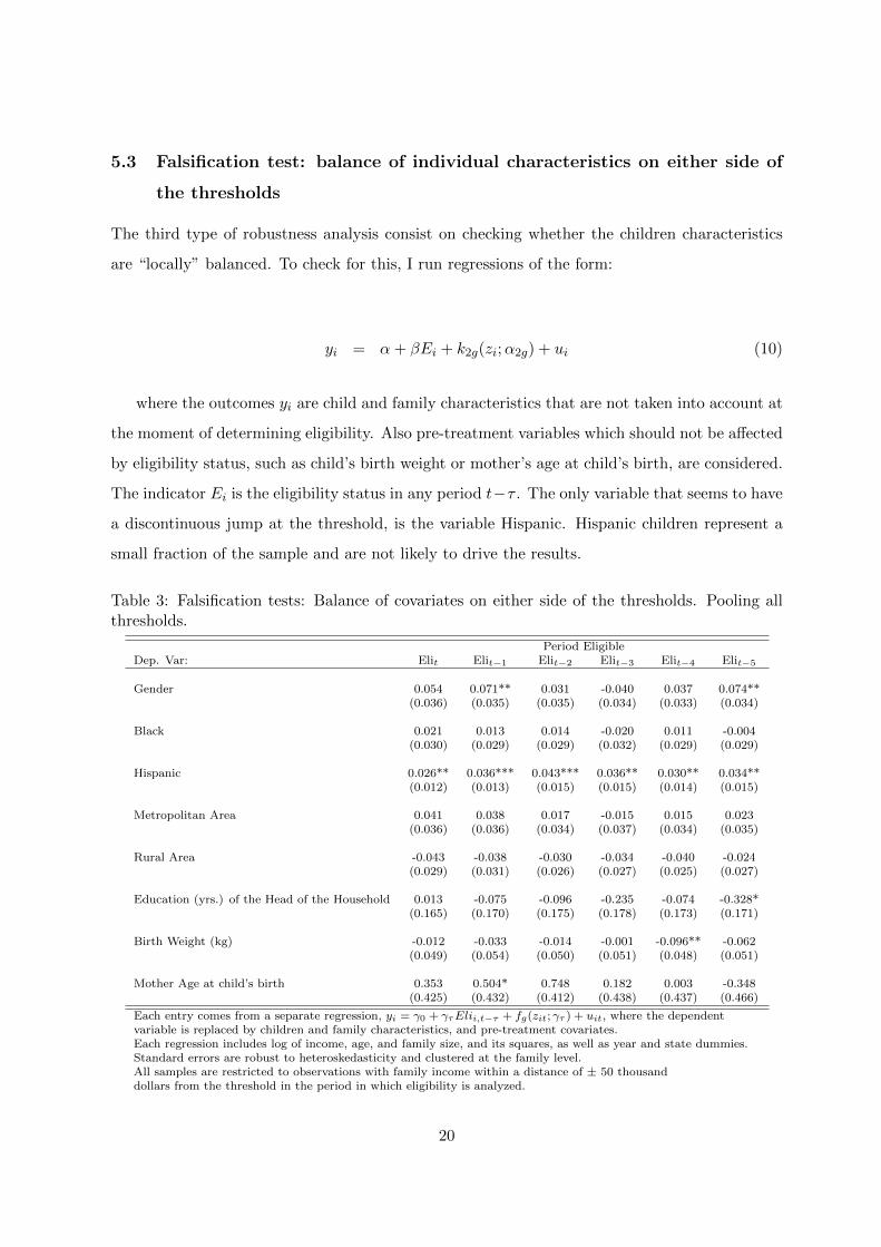
The third type of robustness analysis consist on checking whether the children characteristics

are “locally” balanced. To check for this, I run regressions of the form:

yi = α+ βEi + k2g(zi;α2g) + ui (10)

where the outcomes yi are child and family characteristics that are not taken into account at

the moment of determining eligibility. Also pre-treatment variables which should not be affected

by eligibility status, such as child’s birth weight or mother’s age at child’s birth, are considered.

The indicator Ei is the eligibility status in any period t−τ . The only variable that seems to have

a discontinuous jump at the threshold, is the variable Hispanic. Hispanic children represent a

small fraction of the sample and are not likely to drive the results.

Table 3: Falsification tests: Balance of covariates on either side of the thresholds. Pooling allthresholds.

Period EligibleDep. Var: Elit Elit−1 Elit−2 Elit−3 Elit−4 Elit−5

Gender 0.054 0.071** 0.031 -0.040 0.037 0.074**(0.036) (0.035) (0.035) (0.034) (0.033) (0.034)

Black 0.021 0.013 0.014 -0.020 0.011 -0.004(0.030) (0.029) (0.029) (0.032) (0.029) (0.029)

Hispanic 0.026** 0.036*** 0.043*** 0.036** 0.030** 0.034**(0.012) (0.013) (0.015) (0.015) (0.014) (0.015)

Metropolitan Area 0.041 0.038 0.017 -0.015 0.015 0.023(0.036) (0.036) (0.034) (0.037) (0.034) (0.035)

Rural Area -0.043 -0.038 -0.030 -0.034 -0.040 -0.024(0.029) (0.031) (0.026) (0.027) (0.025) (0.027)

Education (yrs.) of the Head of the Household 0.013 -0.075 -0.096 -0.235 -0.074 -0.328*(0.165) (0.170) (0.175) (0.178) (0.173) (0.171)

Birth Weight (kg) -0.012 -0.033 -0.014 -0.001 -0.096** -0.062(0.049) (0.054) (0.050) (0.051) (0.048) (0.051)

Mother Age at child’s birth 0.353 0.504* 0.748 0.182 0.003 -0.348(0.425) (0.432) (0.412) (0.438) (0.437) (0.466)

Each entry comes from a separate regression, yi = γ0 + γτElii,t−τ + fg(zit; γτ ) + uit, where the dependentvariable is replaced by children and family characteristics, and pre-treatment covariates.Each regression includes log of income, age, and family size, and its squares, as well as year and state dummies.Standard errors are robust to heteroskedasticity and clustered at the family level.All samples are restricted to observations with family income within a distance of ± 50 thousanddollars from the threshold in the period in which eligibility is analyzed.

20

6 Results

6.1 Contemporaneous effects on utilization and health

The models for utilization of preventive medical care are presented in table 4. All models

reported in this table are linear probability models that control for flexible functions of income,

child age, and family size. The first column reports estimates for the full sample, which pools

all the eligibility thresholds. The effects reported in this column are thus average effects across

thresholds. OLS estimates show a positive correlation between having Medicaid coverage and

health care utilization. The intention to treat estimate in the third row shows that making

a child eligible for Medicaid slightly increase health care utilization by 4.4 percentage points;

the IV estimate, however, indicates that the average effect for the subpopulation of compliers

−those who, made eligible for Medicaid, would enroll into the program− rises to 35 percentage

points. These estimates are, however, not statistically significant.

In columns 2 and 3, I do the same estimation, but dividing the sample in two subgroups,

according to the thresholds levels: states with thresholds under 185% of poverty line, and states

with thresholds between 185 and 250%. I do not estimate the effects for thresholds above 250%

of the poverty line, because I showed that Medicaid eligibility does not predict participation for

individuals in the neighborhood of these thresholds. Medicaid eligibility induces a 12 percentage

points increase in utilization for poorer children, with an average effect of 63 percentage points

increase for compliers. For relatively richer children, there is not a statistically significant impact

of Medicaid eligibility on utilization. Also the sign of the point estimates are negative.

The results for the contemporaneous effects of Medicaid on children’s health are presented in

table 5. Panel A of the table presents the ITT estimates, while Panel B shows the IV estimates,

which are the LATE estimates. The first two outcomes are the objective measures of health -

Obese and Overweight. These measures should not be contaminated from effects of “perception”

due to an increase in physician contacts or to a change in health care quality associated with

access to Medicaid. The other two measures are subjective health outcomes.

21

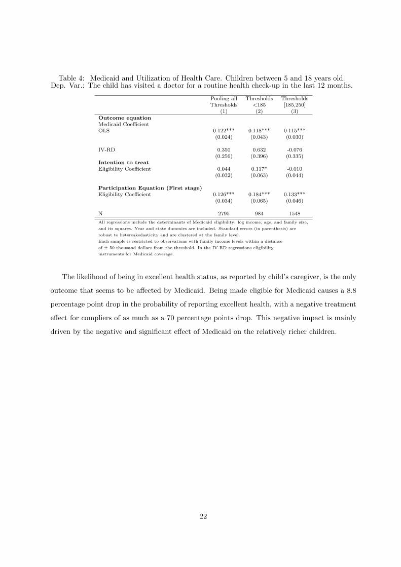
Table 4: Medicaid and Utilization of Health Care. Children between 5 and 18 years old.Dep. Var.: The child has visited a doctor for a routine health check-up in the last 12 months.

Pooling all Thresholds ThresholdsThresholds <185 [185,250]

(1) (2) (3)Outcome equationMedicaid CoefficientOLS 0.122*** 0.118*** 0.115***

(0.024) (0.043) (0.030)

IV-RD 0.350 0.632 -0.076(0.256) (0.396) (0.335)

Intention to treatEligibility Coefficient 0.044 0.117* -0.010

(0.032) (0.063) (0.044)

Participation Equation (First stage)Eligibility Coefficient 0.126*** 0.184*** 0.133***

(0.034) (0.065) (0.046)

N 2795 984 1548

All regressions include the determinants of Medicaid eligibility: log income, age, and family size,

and its squares. Year and state dummies are included. Standard errors (in parenthesis) are

robust to heteroskedasticity and are clustered at the family level.

Each sample is restricted to observations with family income levels within a distance

of ± 50 thousand dollars from the threshold. In the IV-RD regressions eligibility

instruments for Medicaid coverage.

The likelihood of being in excellent health status, as reported by child’s caregiver, is the only

outcome that seems to be affected by Medicaid. Being made eligible for Medicaid causes a 8.8

percentage point drop in the probability of reporting excellent health, with a negative treatment

effect for compliers of as much as a 70 percentage points drop. This negative impact is mainly

driven by the negative and significant effect of Medicaid on the relatively richer children.

22

Table 5: Medicaid and Health outcomes. Contemporaneous effects.Children between 5 and 18 years old.

Pooling All Thresholds ThresholdsDep. Var.: Thresholds <185 [185-250]

(1) (2) (3)

A. ITT

Obese -0.027 -0.067 -0.002(0.030) (0.054) (0.041)

Overweight 0.035 0.060 0.015(0.024) (0.047) (0.033)

Days school missed (> 5) due to illness -0.014 -0.019 -0.031(0.022) (0.047) (0.030)

Health Excellent -0.088** -0.086 -0.125**(0.035) (0.064) (0.050)

B. IV-RD

Obese -0.217 -0.363 -0.017(0.249) (0.323) (0.311)

Overweight 0.277 0.326 0.116(0.206) (0.269) (0.256)

Days school missed (> 5) due to illness -0.110 -0.104 -0.232(0.180) (0.258) (0.245)

Health Excellent -0.698** -0.467 -0.938**(0.336) (0.386) (0.508)

N 2795 984 1548

Each entry comes from a separate regression. All regressions include the determinants

of Medicaid eligibility: log income, age, and family size, and its squares. Year and state

dummies are included. Standard errors (in parenthesis) are robust to heteroskedasticity and

clustered at the family level. Each sample is restricted to observations with family income

levels within a distance of ± 50 thousand dollars from the threshold. In the IV-RD regressions

eligibility instruments for Medicaid coverage.

23

6.2 Lagged effects on health

The finding that Medicaid eligibility and coverage have no statistically significant contempora-

neous effect over health - with the only exception of a negative effect on the parent’s evaluation

of child’s health-, may reflect the fact that health is a stock, and the effects of health insurance

coverage on this health stock may be observed with some lag.

Table 6 reports the IIT estimates, which capture the effect of making a child randomly

eligible for Medicaid in a given period, on outcomes after τ periods, for a sample that pools all

income thresholds. Remember that the ITT estimate identifies the effects of eligibility in one

moment of time on future outcomes, without controlling for behavioral changes in the period

between assignment and when outcomes are measured. Thus, IIT estimates reflect accumulated

effects.

The results in table 6 suggest that Medicaid eligibility neither induced, on average, better

outcomes in the medium (1 to 3 year after) or in the long run (4 and 5 years after). Moreover, in

the medium term, some health measures seems to be negatively affected by Medicaid eligibility.

In particular, being made eligible for Medicaid increases the probability of being obese by 8.5

percentage points and decreases the probability of having excellent health by 8.4 percentage

points, after two years. Being made eligible for Medicaid increases the probability of being obese

by 5.4 percentage points after three years. On average, Medicaid does not have a significant

effect on the probability of missing more than 5 days of school days due to illness. Eligibility

seems to have almost no effects on any of the measures considered after 4 or 5 years.

24

Table 6: Lagged Medicaid Eligibility and Children’s Health. Lagged Intent to Treat (ITT)Effects. Children between 5 and 18 years old. All thresholds.

Average Objective Measures Subjective MeasuresTime elapsed Average Age threshold Obese Overweight School days Excellent

when eligible when eligible Missed (>5) health(1) (2) (3) (4) (5) (6)

0 years ( θ0) 11.1 184.9 -0.027 0.035 -0.014 -0.088**(0.030) (0.024) (0.022) (0.035)

1 years ( θ1) 10.0 184.8 -0.006 0.018 0.021 -0.061*(0.027) (0.023) (0.022) (0.034)

2 years ( θ2) 9.0 174.7 0.085*** -0.009 0.006 -0.084**(0.029) (0.023) (0.024) (0.037)

3 years ( θ3) 8.0 166.8 0.054* -0.033 -0.005 -0.060(0.030) (0.024) (0.023) (0.038)

4 years ( θ4) 7.0 168.3 0.033 0.025 -0.022 0.007(0.029) (0.024) (0.020) (0.036)

5 years ( θ5) 6.0 156.2 0.034 0.001 -0.011 -0.022(0.029) (0.025) (0.021) (0.038)

Each entry comes from a separate regression, yit = α+ θτElii,t−τ + fg(zi,t−τ ; γτ ) + uit.Regressions controls for log of income, age, and family size, and its squares in period t− τ , as wellas year and state dummies. Standard errors are robust to heteroskedasticity and clustered at thefamily level. All samples are restricted to observations with family income within a distance of± 50 thousand dollars from the threshold in period t− τ . Columns 2 and 3 report the averagechildren’s age and the average threshold in period t− τ .

6.3 Heterogeneous lagged effects

In order to investigate whether the lagged effects are heterogeneous across different thresholds,

I split again the sample into two income subgroups: thresholds below 185% of the poverty line,

and thresholds between 185 and 250%.15 Results are shown in tables 7 to 9. I also disaggregate

effects by ages: 5 to 11, and 12 to 18-years old subgroups.

The comparison between the two income subgroups, shows a good deal of heterogeneity of

the impact of Medicaid depending of children’s family income level, as well as a differentials

effect for children of different age groups. This heterogeneity highlights the importance of doing

this disaggregation to draw any conclusions about the lagged effects of Medicaid.

6.3.1 Objective health measures: obesity and overweight

Table 7 presents the lagged effects of Medicaid eligibility on measures of weight status, by level

of income threshold and by age groups. Medicaid eligibility tends to have a negative impact

15Again, I drop the thresholds above 250% of the poverty line, because for this group I cannot find evidencethat eligibility induces, at the threshold, an increase in Medicaid participation rates

25

for children in the the higher-income subgroup −185 and 250% of poverty line− in this health

dimension, since it increases the probability of obesity by 7.8 and 9.4 percentage points, after

2 and 3 years, respectively (column 4, panel B). It also has a positive and significant effect on

the probability of being overweight- a 8.3 percentage point increase- after 4 years. In contrast,

for poorer children, the only negative effect of Medicaid is found 2 years later, as it increases

the probability of obesity by 10 percentage points (column 1, panel B). The rest of the lagged

effects estimated, both on obesity and overweight, are not statistically significant.

Interestingly, looking at different age subgroups I find that Medicaid eligibility has beneficial

effects for poorer children aged 12-18. Being eligible for Medicaid reduces the likelihood of being

overweight for this group by 14.5 percentage points after two years; however this effect is almost

offset by with a rise in the probability of being obese, which increases by 11.3 percentage points,

but the effect is not statistically significant (column 3). Moreover, for this subgroup, Medicaid

eligibility systematically reduces both the probability of being obese or overweight after 4 and 5

years, although the point estimates are not statistically different from zero. For poorer children

with ages between 5 and 11 (column 2), in contrast, the only statistically significant effect is an

increase in the probability of being obese after 2 years of being eligible. For children of higher-

income families, the negative impact of Medicaid eligibility on measures of obesity is driven by

the negative impact it has on the subgroup of children between 5 and 11 years old (column 5).

26

Table 7: Lagged Medicaid Eligibility and Children’s Health. Lagged Intent to Treat (ITT)Effects on Objective Measures of Health, by level of Income Thresholds and by Age Group.

Thresholds<185% Thresholds[185-250]%Time Elapsed 5-18 years old 5-11 years old 12-18 years old 5-18 years old 5-11 years old 12-18 years old

(1) (2) (3) (4) (5) (6)

A. Overweight0 years ( θ0) 0.060 0.070 -0.144 0.015 0.058 -0.087

(0.047) (0.053) (0.107) (0.033) (0.047) (0.298)

1 years ( θ1) -0.0001 0.021 -0.157 0.013 0.050 -0.022(0.043) (0.048) (0.101) (0.032) (0.043) (0.048)

2 years ( θ2) -0.037 -0.018 -0.145* -0.015 0.015 -0.073(0.039) (0.046) (0.080) (0.035) (0.047) (0.052)

3 years ( θ3) -0.041 -0.034 -0.062 -0.007 -0.003 -0.024(0.039) (0.046) (0.067) (0.038) (0.056) (0.057)

4 years ( θ4) -0.006 0.002 -0.050 0.083** 0.076 0.071(0.037) (0.043) (0.071) (0.040) (0.062) (0.051)

5 years ( θ5) -0.012 0.011 -0.078 0.025 -0.015 0.089(0.036) (0.045) (0.065) (0.046) (0.062) (0.063)

B. Obesity0 years ( θ0) -0.067 -0.027 -0.184 -0.002 -0.002 0.035

(0.054) (0.060) (0.121) (0.041) (0.053) (0.069)

1 years ( θ1) 0.037 0.048 -0.001 -0.005 0.003 -0.005(0.052) (0.056) (0.122) (0.038) (0.049) (0.066)

2 years ( θ2) 0.101** 0.103* 0.113 0.078* 0.126** 0.028(0.050) (0.053) (0.118) (0.045) (0.057) (0.070)

3 years ( θ3) -0.014 -0.024 0.015 0.094* 0.124** 0.050(0.045) (0.052) (0.101) (0.048) (0.063) (0.078)

4 years ( θ4) 0.039 0.080 -0.139 -0.005 0.019 0.015(0.043) (0.051) (0.085) (0.047) (0.064) (0.076)

5 years ( θ5) 0.034 0.028 -0.025 0.021 0.088 -0.019(0.040) (0.045) (0.080) (0.054) (0.068) (0.090)

Each entry comes from a separate regression, yit = α+ θτElii,t−τ + fg(zi,t−τ ; γτ ) + uit. Regressions controls forlog of income, age, and family size, and its squares in period t− τ , as well as year and state dummies. Standard errorsare robust to heteroskedasticity and clustered at the family level. All samples are restricted to observations withfamily income within a distance of ± 50 thousand dollars from the threshold in period t− τ .

6.3.2 Subjective health measures

Medicaid also seems to have heterogeneous effects on each on the subjective health measures at

different threshold levels.

Excellent Health. Table 8 reports the lagged effects of Medicaid on the probability of

having excellent health. A negative and statistically significant effect −i.e. a reduction in

the probability of having excellent health− is only observed for children in the higher-income

27

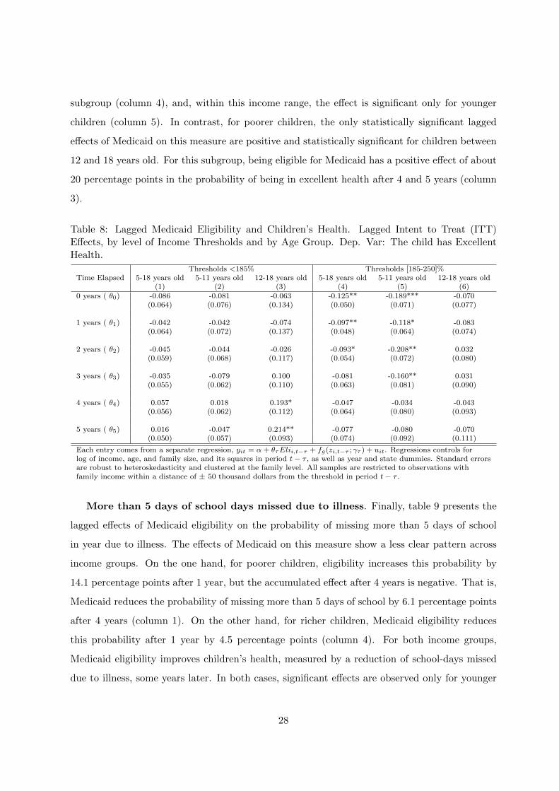
subgroup (column 4), and, within this income range, the effect is significant only for younger

children (column 5). In contrast, for poorer children, the only statistically significant lagged

effects of Medicaid on this measure are positive and statistically significant for children between

12 and 18 years old. For this subgroup, being eligible for Medicaid has a positive effect of about

20 percentage points in the probability of being in excellent health after 4 and 5 years (column

3).

Table 8: Lagged Medicaid Eligibility and Children’s Health. Lagged Intent to Treat (ITT)Effects, by level of Income Thresholds and by Age Group. Dep. Var: The child has ExcellentHealth.

Thresholds <185% Thresholds [185-250]%Time Elapsed 5-18 years old 5-11 years old 12-18 years old 5-18 years old 5-11 years old 12-18 years old

(1) (2) (3) (4) (5) (6)0 years ( θ0) -0.086 -0.081 -0.063 -0.125** -0.189*** -0.070

(0.064) (0.076) (0.134) (0.050) (0.071) (0.077)

1 years ( θ1) -0.042 -0.042 -0.074 -0.097** -0.118* -0.083(0.064) (0.072) (0.137) (0.048) (0.064) (0.074)

2 years ( θ2) -0.045 -0.044 -0.026 -0.093* -0.208** 0.032(0.059) (0.068) (0.117) (0.054) (0.072) (0.080)

3 years ( θ3) -0.035 -0.079 0.100 -0.081 -0.160** 0.031(0.055) (0.062) (0.110) (0.063) (0.081) (0.090)

4 years ( θ4) 0.057 0.018 0.193* -0.047 -0.034 -0.043(0.056) (0.062) (0.112) (0.064) (0.080) (0.093)

5 years ( θ5) 0.016 -0.047 0.214** -0.077 -0.080 -0.070(0.050) (0.057) (0.093) (0.074) (0.092) (0.111)

Each entry comes from a separate regression, yit = α+ θτElii,t−τ + fg(zi,t−τ ; γτ ) + uit. Regressions controls forlog of income, age, and family size, and its squares in period t− τ , as well as year and state dummies. Standard errorsare robust to heteroskedasticity and clustered at the family level. All samples are restricted to observations withfamily income within a distance of ± 50 thousand dollars from the threshold in period t− τ .

More than 5 days of school days missed due to illness. Finally, table 9 presents the

lagged effects of Medicaid eligibility on the probability of missing more than 5 days of school

in year due to illness. The effects of Medicaid on this measure show a less clear pattern across

income groups. On the one hand, for poorer children, eligibility increases this probability by

14.1 percentage points after 1 year, but the accumulated effect after 4 years is negative. That is,

Medicaid reduces the probability of missing more than 5 days of school by 6.1 percentage points

after 4 years (column 1). On the other hand, for richer children, Medicaid eligibility reduces

this probability after 1 year by 4.5 percentage points (column 4). For both income groups,

Medicaid eligibility improves children’s health, measured by a reduction of school-days missed

due to illness, some years later. In both cases, significant effects are observed only for younger

28

children, 5-11 years old (columns 2 and 5).

Table 9: Lagged Medicaid Eligibility and Children’s Health. Lagged Intent to Treat (ITT)Effects, by level of Income Thresholds and by Age Group. Dep. Var: More the 5 days of schoolmissed in the last 12 months due to illness.

Thresholds <185% Thresholds [185-250]%Time Elapsed 5-18 years old 5-11 years old 12-18 years old 5-18 years old 5-11 years old 12-18 years old

(1) (2) (3) (4) (5) (6)0 years ( θ0) -0.019 -0.003 -0.117 -0.031 -0.013 -0.006

(0.047) (0.052) (0.136) (0.030) (0.044) (0.047

1 years ( θ1) 0.141*** 0.134*** 0.133 -0.045* -0.048 -0.019(0.048) (0.049) (0.116) (0.027) (0.040) (0.039)

2 years ( θ2) 0.059 0.049 0.041 -0.057 -0.088* -0.019(0.037) (0.041) (0.083) (0.035) (0.049) (0.044)

3 years ( θ3) 0.002 -0.025 0.054 -0.006 -0.004 -0.034(0.037) (0.043) (0.065) (0.037) (0.048) (0.051)

4 years ( θ4) -0.061* -0.092* -0.003 0.045 0.062 0.023(0.035) (0.042) (0.066) (0.035) (0.049) (0.052)

5 years ( θ5) -0.041 -0.052 -0.012 0.008 0.004 0.017(0.031) (0.038) (0.061) (0.044) (0.059) (0.070)

Each entry comes from a separate regression, yit = α+ θτElii,t−τ + fg(zi,t−τ ; γτ ) + uit. Regressions controls forlog of income, age, and family size, and its squares in period t− τ , as well as year and state dummies. Standard errorsare robust to heteroskedasticity and clustered at the family level. All samples are restricted to observations withfamily income within a distance of ± 50 thousand dollars from the threshold in period t− τ .

29

7 Discussion and Conclusion

The main message from previous results is that Medicaid eligibility has heterogeneous lagged

effects across different income thresholds and also for different age groups. Particularly, in terms

of objective health measures, we saw that Medicaid eligibility has beneficial effects in reducing

obesity and risk of overweight −the two objective health measures analyzed− for children with

family income below 185% of the poverty line aged between 12 and 18 years old. However, I

do not find significant effects for younger children in this income range, nor for children with

family income between 185 and 250% of the poverty line. The heterogeneous effects of Medicaid

on health care utilization across income groups may help to explain this pattern.

On the one hand, we saw that Medicaid coverage tends to increase poorer children’s - under

185% of poverty line- likelihood of visiting a doctor for a routine check up −which may include

a weight check up. Given that the contact with doctors for preventive purposes increases, then

the heterogeneous effects on measures of obesity and overweight for older and younger children

in this income range, may be explained by how they and their families respond to physicians’

recommendations. One can imagine that in case of a child being obese or overweight, the

physician may recommend improving the quality of the diet and increasing the time devoted to

physical activity. For younger children, the effectiveness of these recommendations may depend

more on parents rather than children’s decisions. If parents do not follow the recommendations,

young children rarely will follow them by themselves. But, changing the diet and healthy

behaviors of relatively poorer parents could be a difficult task, which may explain why no

significant effects are observed for younger poorer children. However, older children may have

greater control on their diet and physical activity, which may allow them to adapt better to

physician’s recommendations. This, in turn, is reflected in a beneficial effect of Medicaid in

reducing poorer older children’s obesity and overweight.

On the other hand, health care utilization analysis showed that children with family income

between 185 and 250% of the poverty line do not increase the probability of visiting a doctor

for a routine check-up in response to Medicaid coverage. Moreover, although not significant,

the point estimate was negative. This negligible effect on utilization could be because many of

these children had previous access to health care through private health insurance. Hence, the

switch to the public system do not affect their contact with physicians. However, the quality

of services provided by the public insurance may differ from the quality they received with the

30

private insurance. Indeed, if the quality of physicians who serve Medicaid patients is worse, this

may be reflected in worse children’s health outcomes, relative to the the counterfactual situation

of having private insurance. This explanation could be consistent with the finding that Medicaid

eligibility induces worse results in terms of obesity and overweight for children in this range of

income.

Also consistent with this story is the finding that Medicaid has a negative effect on the

probability of having excellent health, according to parents’ reports, only among children in the

higher-income group. Again, higher-income families who enroll their children into Medicaid are

more likely to have switched from private insurance when made eligible for the public insurance.

These families may find the quality of services they receive with public coverage worse than

quality they received with private coverage, hence their perception about their children’s health

may capture this effect and which is then reflected in a drop of the probability of reporting

excellent health. This is less likely to have happened with poorer families, because they are

more likely to be either uninsured or to have only basic private coverage if the Medicaid option

is not available. This means that, in relative terms, higher-income families who take the public

benefit are more likely to be scarifying a higher level of health care quality than poorer families.

Finally, another interesting finding is the effect of Medicaid on the probability of missing

more than 5 days of school due to illness. The results indicate that Medicaid only affects children

between 5 and 11 years old. For poorer children, Medicaid eligibility increases this probability

after 1 year, but it reduces it after 4 periods. For children in higher income-families, the reduction

occurs after 2 years of being eligible. This result suggests that at some point, Medicaid may

contribute to the human capital formation of children, by allowing them to prevent illnesses and

to be in better health to attend school.

31

References

Almond, D. and J. Currie (2010): “Human Capital Development Before Age Five,” NBER

Working Papers 15827, National Bureau of Economic Research, Inc.

Card, D. and L. D. Shore-Sheppard (2004): “Using Discontinuous Eligibility Rules to

Identify the Effects of the Federal Medicaid Expansions on Low-Income Children,” The Review

of Economics and Statistics, 86, 752–766.

Carneiro, P. and R. Ginja (2009): “Preventing Behavior Problems in Childhood and Ado-

lescence: Evidence From Head Start,” Unpublished Manuscript.

Cellini, S. R., F. Ferreira, and J. Rothstein (2010): “The Value of School Facility

Investments: Evidence from a Dynamic Regression Discontinuity Design,” The Quarterly

Journal of Economics, 125, 215–261.

Cunningham, P. and A. OMalley (2009): “Do reimbursement delays discourage Medicaid

participation by physicians?” Health Affairs, w17–w28.

Currie, J. (2009): “Healthy, Wealthy, and Wise: Socioeconomic Status, Poor Health in Child-

hood, and Human Capital Development,” Journal of Economic Literature, 47, 87–122.

Currie, J., S. Decker, and W. Lin (2008): “Has public health insurance for older children

reduced disparities in access to care and health outcomes?” Journal of Health Economics, 27,

1567 – 1581.

Currie, J. and J. Gruber (1996): “Health Insurance Eligibility, Utilization of Medical Care,

and Child Health,” The Quarterly Journal of Economics, 111, 431–66.

Cutler, D. M. and J. Gruber (1996): “Does Public Insurance Crowd Out Private Insur-

ance?” The Quarterly Journal of Economics, 111, 391–430.

Decker, S. (2007): “Medicaid physician fees and the quality of medical care of Medicaid

patients in the USA,” Review of Economics of the Household, 5, 95–112.

Grieger, L., S. Danziger, and R. Schoeni (2009): “Accurately measuring the trend in

poverty in the United States using the Panel Study of Income Dynamics,” Journal of Economic

and Social Measurement, 34, 105–117.

32

Gruber, J. and K. Simon (2007): “Crowd-Out Ten Years Later: Have Recent Public Insur-

ance Expansions Crowded Out Private Health Insurance?” Working Paper 12858, National

Bureau of Economic Research.

Hahn, J., P. Todd, and W. Van der Klaauw (2001): “Identification and Estimation of

Treatment Effects with a Regression-Discontinuity Design,” Econometrica, 69, 201–09.

Ham, J. C. and L. Shore-Sheppard (2005): “The effect of Medicaid expansions for low-

income children on Medicaid participation and private insurance coverage: evidence from the

SIPP,” Journal of Public Economics, 89, 57–83.

Imbens, G. W. and J. D. Angrist (1994): “Identification and Estimation of Local Average

Treatment Effects,” Econometrica, 62, pp. 467–475.

Imbens, G. W. and T. Lemieux (2008): “Regression discontinuity designs: A guide to prac-

tice,” Journal of Econometrics, 142, 615 – 635, the regression discontinuity design: Theory

and applications.

Koch, T. (2010): “Using RD Design to Understand Heterogeneity in Health Insurance Crowd-

Out,” Working Paper.

Lee, D. S. and T. Lemieux (2010): “Regression Discontinuity Designs in Economics,” Journal

of Economic Literature, 48, 281–355.

Lo Sasso, A. T. and T. C. Buchmueller (2004): “The effect of the state children’s health

insurance program on health insurance coverage,” Journal of Health Economics, 23, 1059–

1082.

van der Klaauw, W. (2002): “Estimating the Effect of Financial Aid Offers on College Enroll-

ment: A Regression-Discontinuity Approach,” International Economic Review, 43, 1249–1287.

33

8 Appendix

Table 10: Falsification test: Balance of covariates on either side of the thresholds. Sample thresholds < 185 %of Poverty Line.

Period EligibleDep. Var: Elit Elit−1 Elit−2 Elit−3 Elit−4 Elit−5

Gender -0.015 0.012 -0.032 -0.099* 0.009 0.048(0.070 0.065 0.061 0.052 0.053 0.046

Black 0.086 -0.050 -0.056 -0.091* -0.009 0.012(0.061) (0.060) (0.054) (0.047) (0.044) (0.041)

Hispanic -0.010 -0.018 -0.008 0.017 0.007 -0.008(0.011) (0.011) (0.012) (0.012) (0.012) (0.013)

Metropolitan Area 0.115* 0.080 -0.030 -0.045 0.082 0.023(0.065) (0.063) (0.057) (0.055) (0.051) (0.050)

Rural Area -0.120** 0.012 0.033 0.001 -0.046 -0.007(0.049) (0.046) (0.039) (0.040) (0.036) (0.036)

Birth Weight -0.022 -0.086 0.078 0.145* 0.032 0.013(0.123) (0.110) (0.093) (0.075) (0.076) (0.067)

Education (yrs) of Head 0.491* 0.110 0.368 0.007 0.220 -0.038(0.293) (0.282) (0.262) (0.254) (0.255) (0.207)

Mother Age at child’S birth 0.805 0.172 0.650 0.095 0.104 -0.495(0.793) (0.760) (0.676) (0.623) (0.631) (0.591)

Notes: Each entry comes from a separate regression, yi = γ0 + γτElii,t−τ + fg(zit; γτ ) +uit, where individual

and family characteristics, and pre-treatment covariates are the dependent variables in the regression. Each

regression includes log of income, age, and family size, and its squares. Year and state dummies. Standard errors

are robust to heteroskedasticity and clustered at the family level. All samples are restricted to observations with

family income within a distance of ± 50 thousand dollars from the threshold in the period in which eligibility is

analyzed.

34

Table 11: Falsification test: Balance of covariates on either side of the thresholds. Sample thresholds [185-250]% of Poverty Line.

Period EligibleDep. Var: Elit Elit−1 Elit−2 Elit−3 Elit−4 Elit−5

Gender 0.089* 0.116** 0.055 0.008 0.066 0.085(0.050) (0.048) (0.052) (0.056) (0.060) (0.074)

Black 0.034 0.039 0.039 0.032 0.005 0.004(0.043) (0.040) (0.045) (0.051) (0.052) (0.061)

Hispanic 0.026 0.061*** 0.075*** 0.045 0.055 0.022(0.021) (0.021) (0.028) (0.032) (0.035) (0.045)

Metropolitan Area 0.029 0.029 0.014 -0.029 -0.032 0.032(0.056) (0.054) (0.054) (0.059) (0.065) (0.067)

Rural Area -0.054 -0.067 -0.073* -0.045 -0.050 -0.062(0.043) (0.044) (0.044) (0.033) (0.038) (0.052)

Education (yrs) of Head -0.036 -0.187 -0.501* -0.333 -0.319 -0.330(0.251) (0.252) (0.274) (0.327) (0.308) (0.347)

Birth Weight -0.048 -0.004 -0.008 -0.117 -0.324*** -0.210**(0.067) (0.069) (0.076) (0.081) (0.084) (0.094)

Mother Age at child birth 0.187 0.840 0.785 0.954 0.549 -0.5910.616 0.621 0.637 0.782 0.845 0.896

Notes: Each entry comes from a separate regression, yi = γ0 + γτElii,t−τ + fg(zit; γτ ) +uit, where individual

and family characteristics, and pre-treatment covariates are the dependent variables in the regression. Each

regression includes log of income, age, and family size, and its squares. Year and state dummies. Standard errors

are robust to heteroskedasticity and clustered at the family level. All samples are restricted to observations with

family income within a distance of ± 50 thousand dollars from the threshold in the period in which eligibility is

analyzed.

35