The Dynamics of Pendula: An Introduction to Hamiltonian ...mason/research/exp2.pdf · The Dynamics...
18
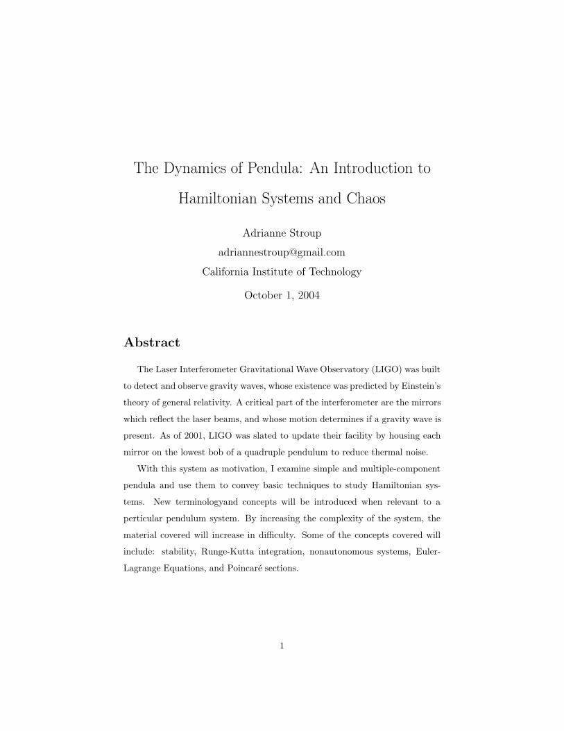
The Dynamics of Pendula: An Introduction to Hamiltonian Systems and Chaos Adrianne Stroup [email protected] California Institute of Technology October 1, 2004 Abstract The Laser Interferometer Gravitational Wave Observatory (LIGO) was built to detect and observe gravity waves, whose existence was predicted by Einstein’s theory of general relativity. A critical part of the interferometer are the mirrors which reflect the laser beams, and whose motion determines if a gravity wave is present. As of 2001, LIGO was slated to update their facility by housing each mirror on the lowest bob of a quadruple pendulum to reduce thermal noise. With this system as motivation, I examine simple and multiple-component pendula and use them to convey basic techniques to study Hamiltonian sys- tems. New terminologyand concepts will be introduced when relevant to a perticular pendulum system. By increasing the complexity of the system, the material covered will increase in difficulty. Some of the concepts covered will include: stability, Runge-Kutta integration, nonautonomous systems, Euler- Lagrange Equations, and Poincar´ e sections. 1
-
Upload
hoangduong -
Category
Documents
-
view
225 -
download
0
Transcript of The Dynamics of Pendula: An Introduction to Hamiltonian ...mason/research/exp2.pdf · The Dynamics...
The Dynamics of Pendula: An Introduction to
Hamiltonian Systems and Chaos
Adrianne Stroup
California Institute of Technology
October 1, 2004
Abstract
The Laser Interferometer Gravitational Wave Observatory (LIGO) was built
to detect and observe gravity waves, whose existence was predicted by Einstein’s
theory of general relativity. A critical part of the interferometer are the mirrors
which reflect the laser beams, and whose motion determines if a gravity wave is
present. As of 2001, LIGO was slated to update their facility by housing each
mirror on the lowest bob of a quadruple pendulum to reduce thermal noise.
With this system as motivation, I examine simple and multiple-component
pendula and use them to convey basic techniques to study Hamiltonian sys-
tems. New terminologyand concepts will be introduced when relevant to a
perticular pendulum system. By increasing the complexity of the system, the
material covered will increase in difficulty. Some of the concepts covered will
include: stability, Runge-Kutta integration, nonautonomous systems, Euler-
Lagrange Equations, and Poincare sections.
1

1 Introduction
Nonlinear dynamics is the study of time-evolving systems governed by equa-
tions where superposition fails [13]. Numerous analytical and numerical tech-
niques have been developed to analyze such dynamical systems.
Even elementary systems introduced in one’s first physics class are nonlinear
in nature. For example, consider the unforced simple pendulum described by
the following differential equation:
θ +g
Lsin θ = 0, (1)
where g is the constant gravitational acceleration, L is the length of the pendu-
lum, and θ is the displaced angle. One uses a small angle approximation (sin x
∼ x+ O(x3) for small x) to approximate the motion of the simple pendulum as
linear. This simplification eliminates several solutions to a pendulum’s motion
such as when a pendulum whirls completely around its pivot [13]. The exact
analytical solution of (1) can be expressed in terms of Jacobian elliptic func-
tions [3], but one can gain a considerable amount of insight by instead using
qualitative methods.
1.1 Hamiltonian Systems
Hamiltonian systems comprise a class of dynamical systems in which some
quantity (typically energy) is constant along the system’s trajectories [3]. Such
systems take the form H(x, p) = constant for some set of displacements and
momenta. The associated dynamical system is given by
x =∂H
∂p,
p = −∂H
∂x, (2)
which are termed Hamiltons’s Equations. The quantity H is called the Hamilto-
nian. If the conserved quantity is energy, it is given by the sum of the potential
and kinetic terms. Hamiltonian systems have an equal number of positions and
2

momenta that describe the motion of the system. Each position-momentum pair
comprises a degree of freedom (dof). The Hamiltonian structure of a system can
be exploited when studying dynamics [16].
Undamped pendula are canonical examples of Hamiltonian systems. The dy-
namics of multiple-component pendula are of great practical interest, as evinced
by GEO 600, a gravity wave detection facility in Germany that uses triple pen-
dula to reduce thermal noise in their interferometers [12]. Additionally the Laser
Interferometer Gravitational Wave Observatory (LIGO) was built to detect and
observe gravity waves, whose existence was predicted by Einstein’s theory of
general relativity. A critical part of the interferometer are the mirrors which re-
flect the laser beams, and whose motion determines if a gravity wave is present.
As of 2001, LIGO was slated to update their facility by housing each mirror on
the lowest bob of a quadruple pendulum to reduce thermal noise [11]. These
developments have produced scientific interest in the dynamics of triple pendula
[15, 4, 14].
1
m1
m2
m3
L1
L2
L3
3
2
Figure 1: Triple pendulum with mass (m1, m2, m3), length (L1, L2, L3), and
angle (θ1, θ2, θ3) labeled.
To be described as chaotic, a system must satisfy three general criteria [13]:
the motion of the system must be extremely (i.e., exponentially) sensitive to the
3

initial conditions, as small input errors can produce drastically different outputs.
It is impossible to predict the motion of a chaotic system after a short period of
time because of such sensitivity. Second, chaotic systems are recurrent, in that
if one defines a neighborhood (no matter how small) around an initial point
in phase space, the trajectory starting at that point will intersect that neigh-
borhood infinitely many times during its time-evolution. Third, trajectories do
not settle down. As t goes to ∞ the trajectory does not become a fixed point,
periodic orbit, or a quasi-periodic orbit [13].
2 Simple Pendulum
We begin our discussion with some terminology from nonlinear dynamics. In
the autonomous system x = f(x), the phase space is the space with coordinates
(x1, ..., xn), which is is n-dimensional [13]. (Autonomous means the system is
not dependent on time). The trajectories are solutions of the system plotted in
the phase space starting at an initial condition x(0). Along them, the Hamilto-
nian is constant. Equilibria occur at points in phase space that satisfy f = 0,
they are called equilibria because if a trajectory begins at an equilibrium it will
remain there for all time. A plot of all the qualitatively different trajectories is
called a phase portrait [13]. Equilibria determine the appearance of the phase
portrait.
The simple pendulum has one dof. With Newtons laws, one can derive the
equations of motion for the simple pendulum (1).
2.1 Linearization about the Equilibria
Linearization determines the local stability of the equilibrium by computing
if a small disturbance from the equilibrium grows or decays [13]. This is done
by computing the Jacobian matrix for the system at the specified equilibrium.
For the simple pendulum, we begin by writing equation (1) as a pair of first
order differential equations
4

θ = v,
v = − sin θ. (3)
The Jacobian for the simple pendulum is
0 1
− cos θ 0
. (4)
With the Jacobian, a new matrix A can be computed for each of the equilibria.
The equilibria for the simple pendulum are (0, 0) and (π, 0). The matrix A is
the Jacobian matrix solved at one of the equilibria. So at (0, 0), A is
0 1
−1 0
. (5)
From this matrix we can compute the eigenvalues using the characteristic equa-
tion det(A − γI) = 0, where I is the identity matrix. (Solving for γ will yeild
the eigenvalues). At (0, 0), γ =√−1 so the eigenvalues are complex. While at
(π, 0), γ = 1,−1. (Computation of A at (π, 0) is left for the readers). Then, af-
ter solving for the eigenvalues of this matrix the local stability of the equillibria
can be determined depending on the values of the eigenvalues.
2.2 Stability of Equilibria
The two equilibria of the simple pendulum occur at the apex and the lowest
point of the pendulum’s motion. In the previous section, we found the eigen-
values at the origin (the lowest point of the pendulum’s swing) to be complex.
Complex eigenvalues occur when the equilibrium is a center or a spiral. The
distinction is made when the eigenvalues are pure imaginary, when the trace is
equal to zero. (The trace is the addition of the diagonal entries of the matrix).
Otherwise the equilibria is a spiral. The bottom position of a simple pendulum
is a center, for which trajectories nearby are neither attracted nor repelled and
remain in periodic orbits nearby. An equilibrium that is a center is stable. To
5

find the direction of the flow compute a few vectors in the vector field [13]. The
rotation about the equilibria located at the origin (a center) is clockwise.
The pendulum has another equilibrium at θ = π (the top of its motion).
The eigenvalues at this equilibrium are positive and negative. This equilibrium
is a saddle, so trajectories are both attracted and repelled. Saddles are unstable
because of this. With this information and the energy equation (6) of this
system,
12θ2 − cos θ = E, (6)
where θ is the velocity, and E = constant, one obtains a complete qualitative
description of the system’s dynamics (see Figure 2).
2.3 Numerical Analysis of the Simple Pendulum
Numerical integration must be used to complement analytical work because
differential equations can almost never be exactly solved analytically. Using the
Runge-Kutta method [7], we can simulate the single pendulum using Matlab
(Figure 2).
The phase space for the simple pendulum is cylindrical because θ is a periodic
variable. The different saddle points in the phase plane represent the same state,
as indicated by the cylindrical phase space. They are all unstable equilibrium at
the apex of the pendulum’s motion. (When the pendulum is positioned straight
up, any disturbance will cause the pendulum to be repelled from the equilibrium
and swing from the apex).
The trajectory which intersects the saddle forms a separatrix; on either side
of this trajectory the motions are qualitatively different. Trajectories outside the
separatrix correspond to periodic whirling motion, while trajectories inside of
the separatrix are librations. Librations are small oscillations about an equilib-
rium. This is the motion commonly identified with a pendulum: the oscillations
about the origin.
In a cylindrical phase space, the separatrix becomes a homoclinic orbit where
6

the trajectory begins and ends at the same point in phase space. Homoclinic
orbits are common in Hamiltonian systems, but rare in non-conservative sys-
tems. (The separatrix would be a pair of heteroclinic orbits if the phase space
was planar, two trajectories beginning and ending at equilibria).
−4 −3 −2 −1 0 1 2 3 4−2
−1.5
−1
−0.5
0
0.5
1
1.5
2
Figure 2: Phase portrait of the simple pendulum: a plot in the plane (θ, θ) where
θ is from (−π, π]. Theta is a periodic variable. The phase space is divided into
two distinct types of motion by the separatrix: at high energies the pendulum
whirls over the top (outside the separatrix), while at low energies the pendulum
oscillates back and forth.
3 Forced Simple Pendula
3.1 Nonautonomous Systems
The forced simple pendulum is an example of a nonautonomous system, or
a time-dependent system. This is because the forcing function is dependent on
time. It consists of a simple pendulum which is perturbed in some direction, in
this case horizontal. The new Hamiltonian H will simply be the addition of the
old Hamiltonian and a perturbation in the horizontal direction.
H = H0 + ε cos(ωt), (7)
7

where ε is the amplitude of forcing, ω is the freqency of forcing, and t is time.
There is also parametric forcing which corresponds to forcing in the vertical
direction. The equation for a pendulum being shaken up and down is
H = H0 + ε sin(ωt), (8)
but we will focus on horizontal forcing.
The forced simple pendulum has 2 dof, time adds another dof. Actually
there is still much mathematical debate about the number of degrees of freedom.
Many people say that the system has 1 12 degrees of freedom because time is not
an entire position and momentum pair and therefore cannot constitute an entire
degree of freedom [5]. With time dependence, the forced simple pendulum is
represented as a system of three first order differential equations (9).
θ = v
v =−g
Lsin θ + ε cos(ωt)
t = 1, (9)
where θ is the displaced angle, v is the velocity, g is the constant gravitational
acceleration, L is the length of the pendulum, ε is the amplitude of forcing, and
ω is the freqency of forcing. The third equation could also be defined as z = ωt.
3.2 Numerical Analysis
To understand the forced simple pendulum system (9), it is essential to
simulate it numerically. This can be done by using the Runge-Kutta method[7].
The Runge-Kutta method is a fourth-order integration method. Basically, the
Runge Kutta method extrapolates each successive point over a discrete time
interval. This method is prefered by many scientists because of its simplicity
and accuracy [13].
No phase portrait can be derived from the trajectories calculated because
no general qualitative behavior applies to any one area in the phase plane. For
8

−4 −3 −2 −1 0 1 2 3 4−6
−4
−2
0
2
4
6
8
10
Figure 3: This is a sample trajectory from a Runge-Kutta simulation where
x(0) = π2 , y(0) = 0, ω = 3, ε = 5, and run from t = [0, 15] with a time step of
δt = .001.
example, with the simple pendulum, the separatrix separated rotations and
librations. Another method must be used to numerically analyze the motion of
the forced simple pendulum.
3.3 Poincare Sections
The numerical analysis of the forced simple and double pendulum will involve
some new concepts, including Poincare sections, which are created as follows.
Whenever a trajectory meets some ”stopping condition,” all variables (aside
from that used to determine the condition) are plotted. This is repeated for
qualitatively different trajectories. The resulting Poincare section is a map
rather than a vector field; it has one dimension less than the phase space. A
useful analogy is to imagine that a piece of paper is inserted into the phase space
so that the trajectory intersects with it [6]. At such intersections, one marks
the paper; repeating this procedure for qualitatively different trajectories yields
a Poincare section. Poincare sections are useful when analyzing chaotic systems
[13], as they make it easier to understand their dynamics.
It is very important to construct Poincare sections intelligently to be able
to visualize the dynamics of chaotic systems. For example, with periodically
forced single pendula, one defines a Poincare section by plotting the location of
trajectories for t = nT , where T is the forcing period and n > 1 is an integer.
9

−4 −3 −2 −1 0 1 2 3 4−6
−4
−2
0
2
4
6
Figure 4: This plot is shows many places where the forced simple pendulum
exhibits periodic behavior. The axises are (θ, v).
In comparison a Poincare section of a simple pendulum looks exactly like the
phase portrait, this is why Poincare sections are not necessary for non-chaotic
systems.
−4 −2 0 2 4−4
−2
0
2
4
6
8
Figure 5: In comparison to the other figure, this plot is very similar to the phase
plane of the simple pendulum no extra information can be garnered by using
Poincare sections on non-chaotic systems.
4 Double Pendula
For the simple pendulum, the equations of motion were derived using force
balance. For the forced simple pendulum, the equations of motion were derived
by adding a perterbation to the Hamiltonian of the simple pendulum. The dou-
ble pendulum is more complex and force balace would quickly become rigorous.
10

Instead we can derive the equations of motion for the double pendulum using
energy balance producing the equations of motion using the Euler-Lagrange
equations.
4.1 Euler-Lagrange Equations
The Euler-Lagrange equations [3] can be used instead of force balance to
derive equations of motion. Lagrangian and Hamiltonian descriptions are com-
plementary ways to describe physical systems, as one can convert from one to
the other with a Legendre transform [8]. Using the Euler-Lagrange equations we
can derive the equations of motion for the double pendulum by initially defining
the positions of the first and second pendulum bobs:
x1 = L1 sin(θ1),
y1 = L1 cos(θ1),
x2 = L1 sin(θ1) + L2 sin(θ2),
y2 = L1 cos(θ1) + L2 cos(θ2), (10)
where (x1, y1) and (x2, y2) represent the cordinates of the pendulum bob in a
plane, L1 and L2 are the lengths of the arms, and θ1 and θ2 are the displaced
angles. The velocities are the derivatives of the position equations:
x1 = θ1L1 cos(θ1),
y1 = −θ1L1 sin(θ1),
x2 = θ1L1 cos(θ1) + θ′2L2 cos(θ2),
y2 = −θ1L1 sin(θ1) − θ′2L2 sin(θ2). (11)
To understand this, the triple pendulum in Fig. 1 provides a good guide.
These values are then used to compute the kinetic (T ) and potential (V ) ener-
11

gies.
T =2∑
n=1
12mnv2
n
V =2∑
n=1
gmnhn (12)
where mi is the mass of each pendulum bob, vi is the velocity of each bob, g
is the constant gravitational acceleration, and hi is the distance from the local
zero potential of each bob [10]. The kinetic and potential energy are then used
to compute the Lagrangian,
L = T − V , (13)
which gives the Euler-Lagrange equation,
d
dt
(∂
∂θ′n
)− ∂L
∂θn= 0, n ∈ {1, 2}. (14)
The resulting equations of motion are
(m1+m2)L21θ
′′1+m2L1L2θ
′′2 cos(θ1−θ2)+m2L1L2θ
′1θ
′2 sin(θ1−θ2)+gL1 sin θ1(m1+m2) = 0
m2L22θ
′′2 + m2L1L2θ
′′1 cos(θ1 − θ2) − m2L1L2θ
′21 sin(θ1 − θ2) + gm2L2 sin θ2 = 0.
(16)
4.2 Nondimensionalization
An important method of simplifying systems of equations is nondimension-
alization, which reduces the number of parameters by creating dimensionless
ratios [2]. Nondimentionalization makes it easier to determine which combi-
nations of parameters are important to understand the qualitative behavior of
dynamical systems. For the double pendulum, he dimensionless terms M and l
are defined as follows:
M =m2
m1 + m2
12
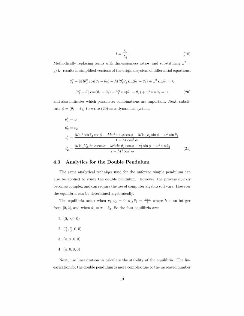
l =L2
L1(18)
Methodically replacing terms with dimensionless ratios, and substituting ω2 =
g/L1 results in simplified versions of the original system of differential equations,
θ′′1 + Mlθ′′2 cos(θ1 − θ2) + Mlθ′1θ′2 sin(θ1 − θ2) + ω2 sin θ1 = 0
lθ′′2 + θ′′1 cos(θ1 − θ2) − θ′21 sin(θ1 − θ2) + ω2 sin θ2 = 0, (20)
and also indicates which parameter combinations are important. Next, substi-
tute φ = (θ1 − θ2) to write (20) as a dynamical system,
θ′1 = v1
θ′2 = v2
v′1 =Mω2 sin θ2 cosφ − Mv2
1 sin φ cosφ − Mlv1v2 sin φ − ω2 sin θ1
1 − M cos2 φ
v′2 =Mlv1V2 sin φ cosφ + ω2 sin θ1 cosφ + v2
1 sin φ − ω2 sin θ2
l − Ml cos2 φ. (21)
4.3 Analytics for the Double Pendulum
The same analytical techniqes used for the unforced simple pendulum can
also be applied to study the double pendulum. However, the process quickly
becomes complex and can require the use of computer algebra software. However
the equilibria can be determined algebraically.
The equilibria occur when v1, v2 = 0, θ1, θ2 = k+π2 where k is an integer
from [0, 2], and when θ1 = π + θ2. So the four equilibria are:
1. (0, 0, 0, 0)
2. (π2 , π
2 , 0, 0)
3. (π, π, 0, 0)
4. (π, 0, 0, 0)
Next, use linearization to calculate the stability of the equilibria. The lin-
earization for the double pendulum is more complex due to the increased number
13

and complexity of the equations of motion. For example, the Jacobian matrix
for the double pendulum is 4 × 4, while for the unforced simple pendulum it
was 2 × 2. To compute the eigenvalues one must compute the determinant of a
4 × 4 matrix, on how to do this see [1].
At this point, it becomes necessary to use computer algebra software. However,
this article is not expositing computer algebra software, so we will pursue an
alternate method of determining the stability of the equilibria.
One can also find stabilities numerically. For example, by looking at the
phase portrait of the simple pendulum once can easily see that the origin is a
stable equilibrium.
4.4 Numerics for the Double Pendulum
The double pendulum is a system of four differential equations and has 2 dof.
The phase space for the double pendulum is four-dimensional. Despite this, the
Runge-Kutta method can be used. However, it is difficult to visualize what is
happening because no graph produced by Matlab can capture all the informa-
tion. One way to visualize the data is by producing four different graphs: (a)
θ1 v. θ2, (b) v1 v. v2, (c) θ1 v. v1, and (d) θ2 v. v2. Figure (6) below is an
example.
Since looking at four graphs at once and deriving useful information from
them is difficult and tedius, we will employ another method to study double
pendula.
4.5 Poincare Sections
For the unforced double pendulum, one can make a Poincare section by
plotting the location of the trajectories when θ1 = 0. This results in a three
dimentional Poincare section. For simplicity’s sake I eliminated one variable
from the maps I produced.
14

(a)−0.8 −0.6 −0.4 −0.2 0 0.2 0.4 0.6 0.8−4
−3
−2
−1
0
1
2
3
4
(b)−4 −3 −2 −1 0 1 2 3 4
17
18
19
20
21
22
23
24
25
(c)−0.8 −0.6 −0.4 −0.2 0 0.2 0.4 0.6 0.8−4
−3
−2
−1
0
1
2
3
4
(d)−4 −3 −2 −1 0 1 2 3 4
17
18
19
20
21
22
23
24
25
Figure 6: This is a compellation of trajectories from a simulation from the
double pendulum. It is difficult to see what the system is doing as a whole, but
graph (c) representing the top bob has a quasi-periodic orbit about its origin,
while graph (d) representing the second bob shows that it is whirling. This
graph had the initial conditions: θ1 = 0, θ2 = 0, v1 = 2, v2 = 20, and run for
10, 000 iterations with a step-size of .001.
Future Considerations
4.6 Triple Pendulum
The equations of motion for the triple pendulum can be derived using the
Euler-Lagrange equations. It is actually the most convenient method especially
since the equations become large.
The triple pendulum has three degrees of freedom. Poincare sections can be
used to analyze the motion of the triple pendulum, however phase space analysis
and perturbation theory are more common techniques when studying chaotic
systems [9]. Also common are perturbative techniques that include averaging
15

−3 −2 −1 0 1 2 3 4−3
−2
−1
0
1
2
3
4
Figure 7: When representing chaotic behavior Poincare sections resemble scatter
plots, with enough iterations, they begin to define and encircle areas that are
non-chaotic and periodic areas.
−3 −2 −1 0 1 2 3−6
−4
−2
0
2
4
6
Figure 8: This is a plot of quasi-periodic areas on the double pendulum’s phase
plane.
and the method of multiple scales. To continue studying chaos and Hamiltonian
systems the autor reccomends researching these methods.
Acknowledgements
I’d like to thank my mentor Mason A. Porter, Ph.D. for all of his time, advice,
and endless patience! Also I’d like to thank my co-mentor Anthony Leonard,
Ph.D for providing realworld examples of the techniques I was studying. I’d
also like to thank the Georgia Institute of Technology for making their resources
available to me for my research.
16

References
[1] Eric Carlen and Conceicao Carvalho. Beggining with linear algebra.
http://www.math.gatech.edu/∼carlen/1502S/cnotes.html.
[2] A.C. Fowler. Mathematical Models in the Applied Sciences. Cambridge
Texts in Applied Mathematics, 1997.
[3] Herbert Goldstein. Classical Mechanics. Addison-Wesley, second edition,
1980.
[4] Erik Neuman. Double pendulum. http://www.myphysicslab.com/dbl pendulum.htm,
Retrieved 27 February 2004.
[5] Martijin van Noort, Mason A. Porter, Yingfei Yi, and Shui-
Nee Chow. Quasiperiodic and chaotic dynamics in bose-einstein
condensates in periodic lattices and superlatticies. arXvi,
(http://arxiv.org/abs/math.DS/0405112), Retrieved 18 September
2004.
[6] Mason A. Porter and Richard L. Liboff. Chaos on the quantum scale.
American Scientist, November-December 2001.
[7] William H. Press, Brian P. Flannery, Saul A. Teukolsky, and William T.
Vetterling. Numerical Recipes: The Art of Scientific Computing. FOR-
TRAN. Cambridge University Press, Cambridge, 1989.
[8] Richard H. Rand. Topics in Nonlinear Dynamics with Computer Algebra,
volume 1 of Computation in Education: Mathematics, Science and Engi-
neering. Gordon and Breach Science Publishers, 1994.
[9] Richard H. Rand. Lecture notes on nonlinear vibrations. Version 45,
http://www.tam.cornell.edu/randdocs/, Retrieved June 17 2004.
[10] Robert Resnick and David Halliday. Physics Part 1. John Wiley and Sons
Inc., New York, 1966.
17

[11] Keith Riles. The ligo experiment present and future.
http://tenaya.physics.lsa.umich.edu/∼keithr/talks/riles aps2004.pdf,
Retrieved 5 July 2004.
[12] N. A. Robertson et al. Quadruple suspension design for advanced LIGO.
Classical and Quantum Gravity, 19:4043–4058, 2002.
[13] Steven H. Strogatz. Nonlinear Dynamics and Chaos. Addison-Wesley, 1994.
[14] University of Bristol. The Single Pendulum.
http://www.enm.bris.ac.uk/teaching/projects/2000 01/tg7360/Single%20Pendulum.htm,
Retrieved 26 February 2004.
[15] Simon Yeung. The triple spherical pendulum. Technical report, Califor-
nia Institute of Technology, December 1995. Division of Chemistry and
Chemical Engineering.
[16] Vadim Zharnitsky. The geometrical description of nonlinear dynamics of a
multiple pendulum. SIAM Journal on Applied Mathematics, 55(6):1753–
1763, 1995.
18