The Dynamic Relationship between Stock Returns, Trading ... · PDF fileThe Dynamic...
49
The Dynamic Relationship between Stock Returns, Trading Volume and Volatility: Evidence from Indian Stock Market Brajesh Kumar 1 Priyanka Singh 2 Abstract This paper empirically examines the relationship between returns, volatility and trading volume for 50 Indian stocks. Three measures of trading volume namely number of transactions, number of shares traded and value of shares traded are used. The contemporaneous correlation between returns and trading volume and asymmetric relation between level of trading volume and returns is examined. The dynamic relation as marked by lead-lag relationship is also investigated between the returns and volume. In case of volatility, the contemporaneous and asymmetric relation is examined between unconditional volatility and volume. The Mixture of Distributions Hypothesis (MDH), which tests the GARCH vs Volume effect, is also studied between the conditional volatility and volume. The evidence for positive contemporaneous relation between returns and volume as well as conditional and unconditional volatility and volume is found. We also find that the level of volume is dependent on the direction of price change only in case of 60% of the stocks in the sample. The results of VAR model, Granger causality, impulse response function and variance decomposition, indicate that in some stocks returns Granger cause trading volume, which is easily conceivable in the context of an emerging market where development of the market causes sequential information dissemination (Assogbavi, 2007). While analyzing the MDH, the results provide mixed conclusions, neither entirely rejecting the MDH nor giving it an unconditional support. Similar kind of result has been found by Ane and Ureche-Rangau (2008) in the context of MDH. It is also found that in Indian stock market, the number of transactions may be a better proxy of information than the number of shares traded and the value of shares traded. Keywords: Trading volume, Volatility, Mixture of distributions hypothesis, GARCH, Granger Causality, VAR, Impulse response function, Variance decomposition 1 Doctoral Student, Indian Institute of Management Ahmedabad, email: [email protected] 2 Doctoral Student, Indian Institute of Management Ahmedabad, email: [email protected] The authors are thankful to Prof. Ajay Pandey, Indian Institute of Management Ahmedabad, for valuable guidance. We also thank the two anonymous referees for their comments on the proposal, which helped in improvising the research undertaken. The views expressed in this paper are that of authors and not necessarily of NSE.
Transcript of The Dynamic Relationship between Stock Returns, Trading ... · PDF fileThe Dynamic...
The Dynamic Relationship between Stock Returns, Trading Volume and Volatility: Evidence from Indian Stock Market
Brajesh Kumar1 Priyanka Singh2
Abstract
This paper empirically examines the relationship between returns, volatility and trading volume for 50
Indian stocks. Three measures of trading volume namely number of transactions, number of shares traded
and value of shares traded are used. The contemporaneous correlation between returns and trading
volume and asymmetric relation between level of trading volume and returns is examined. The dynamic
relation as marked by lead-lag relationship is also investigated between the returns and volume. In case
of volatility, the contemporaneous and asymmetric relation is examined between unconditional volatility
and volume. The Mixture of Distributions Hypothesis (MDH), which tests the GARCH vs Volume effect, is
also studied between the conditional volatility and volume. The evidence for positive contemporaneous
relation between returns and volume as well as conditional and unconditional volatility and volume is
found. We also find that the level of volume is dependent on the direction of price change only in case of
60% of the stocks in the sample. The results of VAR model, Granger causality, impulse response function
and variance decomposition, indicate that in some stocks returns Granger cause trading volume, which is
easily conceivable in the context of an emerging market where development of the market causes
sequential information dissemination (Assogbavi, 2007). While analyzing the MDH, the results provide
mixed conclusions, neither entirely rejecting the MDH nor giving it an unconditional support. Similar
kind of result has been found by Ane and Ureche-Rangau (2008) in the context of MDH. It is also found
that in Indian stock market, the number of transactions may be a better proxy of information than the
number of shares traded and the value of shares traded.
Keywords: Trading volume, Volatility, Mixture of distributions hypothesis, GARCH, Granger
Causality, VAR, Impulse response function, Variance decomposition
1 Doctoral Student, Indian Institute of Management Ahmedabad, email: [email protected]
2 Doctoral Student, Indian Institute of Management Ahmedabad, email: [email protected]
The authors are thankful to Prof. Ajay Pandey, Indian Institute of Management Ahmedabad, for valuable guidance.
We also thank the two anonymous referees for their comments on the proposal, which helped in improvising the
research undertaken. The views expressed in this paper are that of authors and not necessarily of NSE.
2/49
The Dynamic Relationship between Stock Returns, Trading Volume and Volatility: Evidence from Indian Stock Market
1. Introduction
In financial economics, considerable attention has been given to understand the relationship
between return, volatility and trading volume. As argued by Karpoff (1986, 1987), price-volume
relationship is important because this empirical relationship helps in understanding the
competing theories of dissemination of information flow into the market. This may also help in
event (informational event/liquidity event) studies by improving the construction of test and its
validity. This relationship is also critical in assessing the empirical distribution of returns as
many financial models are based on an assumed distribution of return series.
There are extensive empirical studies which support the positive relationship between price,
trading volume and volatility of a tradable asset (Crouch, 1970; Epps and Epps, 1976; Karpoff,
1986 1987, Assogbavi et al., 1995; Chen et al, 2000). Various theoretical models have been
developed to explain the relationship between price and trading volume. These include
sequential arrival of information models (Copeland, 1976; Morse, 1980 and Jennings and Barry,
1983), a mixture of distributions model (Clark, 1973; Epps and Epps, 1976; Tauchen and Pitts,
1983; and Harris, 1986 Lamoureux & Lastrapes, 1990) asymmetric information models (Kyle,
1985; Admati and Pieiderer, 1988), and differences in opinion models (Varian, 1985, 1989;
Harris and Raviv, 1993). All these models advocate the positive relationship between price,
trading volume and volatility. In a similar strand of literature, the asymmetric nature of volume
response to return (volatility) i.e. the trading volume is higher in which price ticks up than
volume on downtick, has been explained (Epps 1975; Karpoff 1987, 1988; Assogbavi et al.,
1995). The asymmetric nature is explained through heterogeneous expectation model and costs
involved in short selling. Recently, Henry and McKenzie (2006) examined the relationship
between volume and volatility allowing for the impact of short sales for Hong-Kong market and
found that the asymmetric bidirectional relationship exists between volatility and volume.
Other than positive contemporaneous relationship between returns and trading volume and
asymmetric relationship between level of volume and price changes, recent studies also report
bidirectional causality between returns and volume (Smirlock and Starks, 1988; Hiemstra and
Jones, 1994; Bhagat and Bhatiya, 1996; Chen, Firth, and Rui, 2001; and Ratner and Leal; 2001).
This dynamic relationship between returns and volume is explained by various theoretical
models. These include models developed by Blume, Easley, and O’Hara (1994), Wang (1994),
He and Wang (1995) and Chordia and Swaminathan (2000). Most of these models assume
volume as a proxy for quality and precision of information. It is found that the information
content of volume and sequential processing of information may lead to dynamic relationship
between returns and trading volume. Blume, Easley, and O’Hara (1994) developed a model in
which prices and volume of the past carry information about the value of security and explained
that the traders who include past volume measures in their technical analysis performed better.
Wang (1994) and He and Wang (1995) developed a model based on asymmetric information and
showed that the trading volume is related to information flow in the market and investor’s
private information is revealed through trading volume. Chordia and Swaminathan (2000) also
3/49
examined the predictability of short-term stock returns based on trading volume and concluded
that high volume stocks respond promptly to market-wide information.
Similar to returns and volume, considerable attention has also been given to understand the
relationship between volatility and trading volume of an asset by the researchers. Most of the
studies report the evidence of ARCH effects in the time series of returns. However, very few of
them try to give the theoretical economic explanation of the autoregressive nature of conditional
volatility. One of the possible theoretical explanations is the mixture of distributions hypothesis
(Clark, 1973; Epps and Epps, 1976; Tauchen and Pitts, 1983; and Lamoureux and Lastrapes,
1990). The Mixture of distributions hypothesis (MDH) explains the positive relationship between
price volatility and trading volume as they jointly depend on a common factor, information
innovation. According to MDH, returns are generated by mixture of distribution and information
arrival is the mixing variable. This mixing variable causes momentum in the squared residual of
daily returns and hence autoregressive nature of the conditional volatility. As, information
arrival is unobserved, trading volume is usually considered as a proxy of information flow into
the market. Any unexpected information affects both volatility and volume contemporaneously
and, therefore volatility and volume are hypothesized to be positively related.
While a fair amount of empirical evidence on the daily returns, volatility and volume
relationship, asymmetric relationship between volume and price change, and mixed distribution
hypothesis exists for developed countries, very few empirical studies have been reported from
emerging markets and specifically from Indian stock market. This paper reports same empirical
evidence on those issues for Indian Stock market which is an order driven continuous market. All
the 50 stocks of S&P CNX Nifty, a value-weighted stock index of National Stock Exchange
(www.nseindia.com), Mumbai, derived from prices of 50 large capitalization stocks, for the
period of 1st January 2000 to 31
st December 2008 are analyzed. We specifically address the
following issues related to relationship between returns, volatility and trading volume in this
paper.
� What kind of relationship exists between trading volume and returns? Is the relationship
asymmetric in nature?
� Do trading volume and returns exhibit dynamic relationship? If yes then, what is
direction and extent of relationship between these variables?
� What kind of relationship exists between trading volume and price volatility
(unconditional)? Is the relationship asymmetric in nature?
� Does there exist ARCH effects in the stock returns? If yes then, is this ARCH effects
diminished or reduced when trading volume is incorporated as an explanatory variable in
the GARCH equation?
The remainder of this paper is organized as follows. A brief review of empirical literature is
given in section 2. Section 3 explains the sample and basic characteristics of the data. The
empirical models of the contemporaneous and dynamic relationship between returns and trading
volume, and models of the mixture of distributions hypothesis are explained in section 4. Section
5 discusses the empirical findings and the last section summarizes them and gives a conclusion.
4/49
2. Literature on Relationship among Returns, Trading Volume and Volatility
There have been number of empirical studies in developed markets that provide evidence on the
relationship between trading volume and stock returns. Crouch (1970) studied the relationship
between daily trading volume and daily absolute changes of market index and individual stocks
and found positive correlation between them. Rogalski (1978) used monthly stock data and Epps
(1975, 1977) used transactions data and found a positive contemporaneous correlation between
trading volume and absolute returns. In an emerging market context, Brailsford (1996) for the
Australian stock market, Saatcioglu and Starks (1998) for Latin America stock market found a
positive contemporaneous relationship between absolute returns and volatility. Smirlock and
Starks (1988) analyzed the dynamic relationship between trading volume and returns using
individual stock transactions data and found a positive lagged relation between volume and
absolute price changes. Using nonlinear Granger causality test, Hiemstra and Jones (1994)
analyzed the bidirectional causality between trading volume and returns for New York Stock
Exchange and found support for positive bidirectional causality between them. However, Bhagat
and Bhatia (1996) found strong one-directional causality running from price changes to trading
volume while analyzing the lead-lag relationship between trading volume and volatility using
Granger causality test. Moosa and Al-Loughani (1995) examined the dynamic relationship
between price and volume for four Asian stock markets excluding India and found a strong
evidence for bi-directional causality for Malaysia, Singapore, and Thailand. Assogbavi (2007)
used vector auto-regression model to analyze dynamic relationship between returns and trading
volume using weekly data of individual equities of the Russian Stock Exchange. They found a
strong evidence of bi-directional relationship between volume and returns.
The relationship between stock return volatility and trading volume has also been analyzed in
several studies. Harris (1987) used the number of transactions as a measure of volume and found
a positive correlation between changes in volume and changes in squared returns for individual
NYSE stocks. In the U.S. stock market, Andersen (1996), Gallo and Pacini (2000), Kim and Kon
(1994), and Lamoureux and Lastrapes (1990, 1994) found support for the MDH. In emerging
markets context, Pyun et al. (2000) investigated 15 individual shares of the Korean stock market,
Brailsford (1996) analyzed the effect of information arrivals on volatility persistence in the
Australian stock market and Lange (1999) for the small Vancouver stock exchange. All of them
found support for the mixed distribution hypothesis. Wang et al. (2005) examined the Chinese
stock market and investigated the dynamic causal relation between stock return volatility and
trading volume. They found support for the MDH as the inclusion of trading volume in the
GARCH specification of volatility reduced the persistence of the conditional variance. In
general, most of empirical studies in the developed and developing market context have found
evidence that the inclusion of trading volume in GARCH models for volatility results in
reduction of the estimated persistence or even causes it to vanish. However, Huang and Yang
(2001) for the Taiwan Stock Market and Ahmed et al. (2005) for the Kuala Lumpur Stock
Exchange found that the persistence in return volatility remains even after volume is included in
the conditional variance equation.
The relationship between volume and volatility has also been studied in the market
microstructure strand of literature. However, the results are not consistent. For example, the
model of Admati and Pfleiderer (1988) which assumes three kinds of traders, informed traders
5/49
who trade on information, discretionary liquidity traders who can choose the time they want to
trade but must satisfy their liquidity demands before the end of the trading day, and non
discretionary traders who transact due to the reasons exogenous at a specific time and don’t have
the flexibility of choosing the trade time, supports the positive relationship between volatility and
trading volume. On the other hand Foster and Viswanathan (1990) model suggests that this
relationship does not necessarily follow even when they use the same classification of traders as
used by Admati and Pfleiderer.
Another very important issue that has been has been addressed by researchers is the
measurement of trading volume. Generally, three kinds of measures, namely, number of trades,
volume of trade or total dollar value of trades have been used as a proxy of volume. The
theoretical models of the past did not support the effect of trade size in the volatility volume
relationship. However, recent models consider the effect of trade size on the volume volatility
relationship but contradictory results. On one hand, some models (Grundy and McNichols, 1989;
Holthausen and Verrecchia, 1990; Kim and Verrecchia, 1991) show that informed traders prefer
to trade large amounts at any given price and hence size is positively related to the quality of
information and is therefore correlated with price volatility. On the other hand, some other
models (Kyle, 1985; Admati and Pfeiderer, 1988) indicate that a monopolist informed trader may
disguise his trading activity by splitting one large trade into several small trades. Thus trade size
may not necessarily convey adverse information.
Given the mixed results between price and trading volume especially in emerging markets
context, some additional results from other emerging financial markets are needed to better
understand the price-volume relationship. Very few studies have examined the price-volume
relationship in Indian market. This paper represents one such attempt to investigate returns,
volatility and trading volume relationship in Indian Stock market.
2. The Sample and its Characteristics
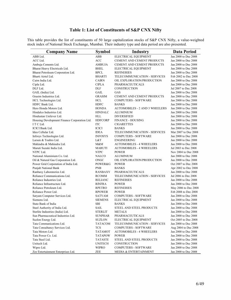
In this study our data set consists of all the stocks of S&P CNX Nifty Index. S&P CNX Nifty is a
well diversified 50 stock index accounting for 21 sectors of the Indian economy. Table 1
provides the list of these companies, industry type and the period considered in the analysis. Data
has been collected for the period of 1st January 2000 to 31
st December 2008. For companies that
were listed after 1st January 2000, the data has been taken from the listing date to 31
st December
2008. The data set consists of 82674 data points of adjusted daily closing prices and three
different measures of daily volume (number of transactions, number of shares traded and total
value of shares). The daily adjusted closing prices have been used for estimating daily returns.
The percentage return of the stock is defined as 100ln1
×
=
−t
tt p
pR , where, Rt is logarithmic
daily percentage return at time t and Pt–1 and Pt are daily price of an asset on two successive days
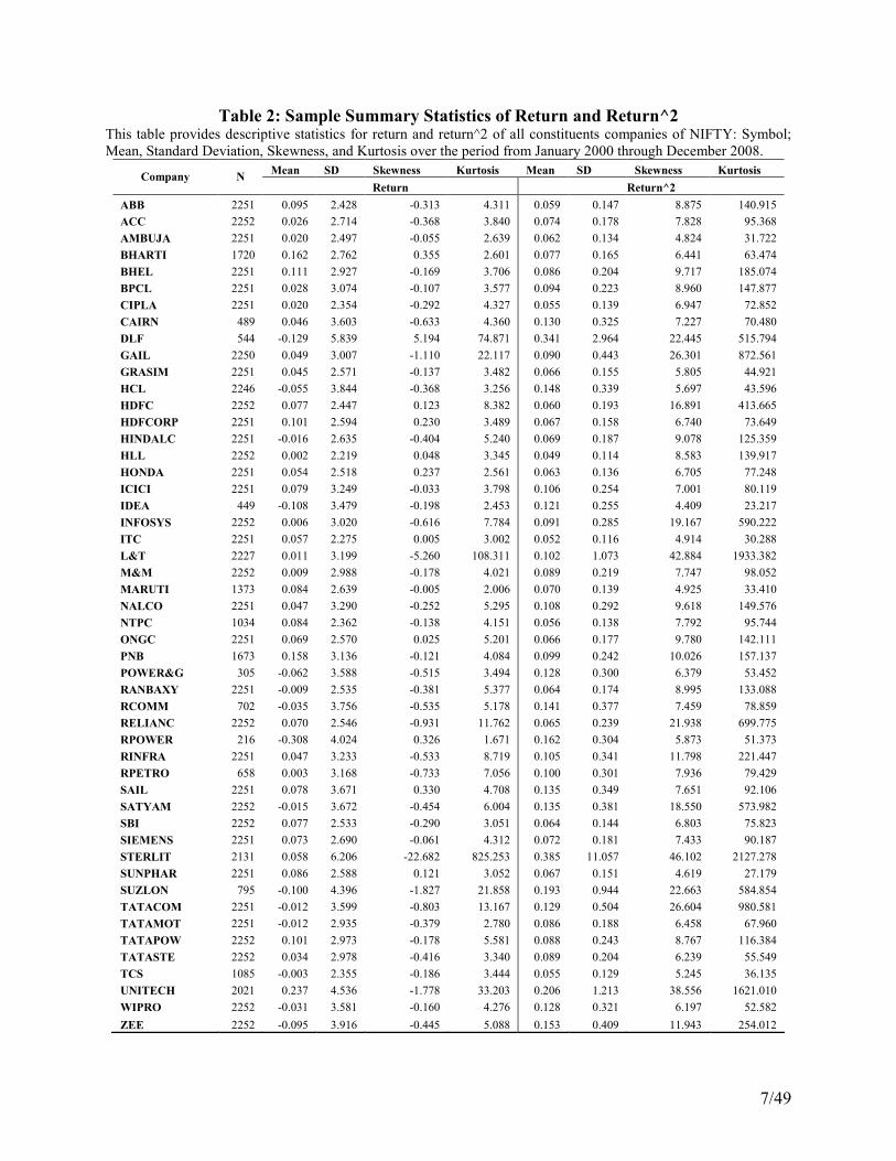
t-1 and t respectively. Table 2 presents the basic statistics relating to the returns and the squared
returns of each stock in the sample.
6/49
Table 1: List of Constituents of S&P CNX Nifty
This table provides the list of constituents of 50 large capitalization stocks of S&P CNX Nifty, a value-weighted
stock index of National Stock Exchange, Mumbai. Their industry type and data period are also presented.
Company Name Symbol Industry Data Period ABB Ltd. ABB ELECTRICAL EQUIPMENT Jan 2000 to Dec 2008
ACC Ltd. ACC CEMENT AND CEMENT PRODUCTS Jan 2000 to Dec 2008
Ambuja Cements Ltd. AMBUJA CEMENT AND CEMENT PRODUCTS Jan 2000 to Dec 2008
Bharat Heavy Electricals Ltd. BHEL ELECTRICAL EQUIPMENT Jan 2000 to Dec 2008
Bharat Petroleum Corporation Ltd. BPCL REFINERIES Jan 2000 to Dec 2008
Bharti Airtel Ltd. BHARTI TELECOMMUNICATION - SERVICES Feb 2002 to Dec 2008
Cairn India Ltd. CAIRN OIL EXPLORATION/PRODUCTION Jan 2000 to Dec 2008
Cipla Ltd. CIPLA PHARMACEUTICALS Jan 2000 to Dec 2008
DLF Ltd. DLF CONSTRUCTION Jul 2007 to Dec 2008
GAIL (India) Ltd. GAIL GAS Jan 2000 to Dec 2008
Grasim Industries Ltd. GRASIM CEMENT AND CEMENT PRODUCTS Jan 2000 to Dec 2008
HCL Technologies Ltd. HCL COMPUTERS - SOFTWARE Jan 2000 to Dec 2008
HDFC Bank Ltd. HDFC BANKS Jan 2000 to Dec 2008
Hero Honda Motors Ltd. HONDA AUTOMOBILES - 2 AND 3 WHEELERS Jan 2000 to Dec 2008
Hindalco Industries Ltd. HINDALC ALUMINIUM Jan 2000 to Dec 2008
Hindustan Unilever Ltd. HLL DIVERSIFIED Jan 2000 to Dec 2008
Housing Development Finance Corporation Ltd. HDFCORP FINANCE - HOUSING Jan 2000 to Dec 2008
I T C Ltd. ITC CIGARETTES Jan 2000 to Dec 2008
ICICI Bank Ltd. ICICI BANKS Jan 2000 to Dec 2008
Idea Cellular Ltd. IDEA TELECOMMUNICATION - SERVICES Mar 2007 to Dec 2008
Infosys Technologies Ltd. INFOSYS COMPUTERS - SOFTWARE Jan 2000 to Dec 2008
Larsen & Toubro Ltd. L&T ENGINEERING Jan 2000 to Dec 2008
Mahindra & Mahindra Ltd. M&M AUTOMOBILES - 4 WHEELERS Jan 2000 to Dec 2008
Maruti Suzuki India Ltd. MARUTI AUTOMOBILES - 4 WHEELERS Jul 2003 to Dec 2008
NTPC Ltd. NTPC POWER Nov 2004 to Dec 2008
National Aluminium Co. Ltd. NALCO ALUMINIUM Jan 2000 to Dec 2008
Oil & Natural Gas Corporation Ltd. ONGC OIL EXPLORATION/PRODUCTION Jan 2000 to Dec 2008
Power Grid Corporation of India Ltd. POWER&G POWER Oct 2007 to Dec 2008
Punjab National Bank PNB BANKS Apr 2002 to Dec 2008
Ranbaxy Laboratories Ltd. RANBAXY PHARMACEUTICALS Jan 2000 to Dec 2008
Reliance Communications Ltd. RCOMM TELECOMMUNICATION - SERVICES Jul 2006 to Dec 2008
Reliance Industries Ltd. RELIANC REFINERIES Jan 2000 to Dec 2008
Reliance Infrastructure Ltd. RINFRA POWER Jan 2000 to Dec 2008
Reliance Petroleum Ltd. RPETRO REFINERIES May 2006 to Dec 2008
Reliance Power Ltd. RPOWER POWER Feb 2008 to Dec 2008
Satyam Computer Services Ltd. SATYAM COMPUTERS - SOFTWARE Jan 2000 to Dec 2008
Siemens Ltd. SIEMENS ELECTRICAL EQUIPMENT Jan 2000 to Dec 2008
State Bank of India SBI BANKS Jan 2000 to Dec 2008
Steel Authority of India Ltd. SAIL STEEL AND STEEL PRODUCTS Jan 2000 to Dec 2008
Sterlite Industries (India) Ltd. STERLIT METALS Jan 2000 to Dec 2008
Sun Pharmaceutical Industries Ltd. SUNPHAR PHARMACEUTICALS Jan 2000 to Dec 2008
Suzlon Energy Ltd. SUZLON ELECTRICAL EQUIPMENT Oct 2005 to Dec 2008
Tata Communications Ltd. TATACOM TELECOMMUNICATION - SERVICES Jan 2000 to Dec 2008
Tata Consultancy Services Ltd. TCS COMPUTERS - SOFTWARE Aug 2004 to Dec 2008
Tata Motors Ltd. TATAMOT AUTOMOBILES - 4 WHEELERS Jan 2000 to Dec 2008
Tata Power Co. Ltd. TATAPOW POWER Jan 2000 to Dec 2008
Tata Steel Ltd. TATASTE STEEL AND STEEL PRODUCTS Jan 2000 to Dec 2008
Unitech Ltd. UNITECH CONSTRUCTION Jan 2000 to Dec 2008
Wipro Ltd. WIPRO COMPUTERS - SOFTWARE Jan 2000 to Dec 2008
Zee Entertainment Enterprises Ltd. ZEE MEDIA & ENTERTAINMENT Jan 2000 to Dec 2008
7/49
Table 2: Sample Summary Statistics of Return and Return^2 This table provides descriptive statistics for return and return^2 of all constituents companies of NIFTY: Symbol;
Mean, Standard Deviation, Skewness, and Kurtosis over the period from January 2000 through December 2008.
Mean SD Skewness Kurtosis Mean SD Skewness Kurtosis Company N
Return Return^2
ABB 2251 0.095 2.428 -0.313 4.311 0.059 0.147 8.875 140.915
ACC 2252 0.026 2.714 -0.368 3.840 0.074 0.178 7.828 95.368
AMBUJA 2251 0.020 2.497 -0.055 2.639 0.062 0.134 4.824 31.722
BHARTI 1720 0.162 2.762 0.355 2.601 0.077 0.165 6.441 63.474
BHEL 2251 0.111 2.927 -0.169 3.706 0.086 0.204 9.717 185.074
BPCL 2251 0.028 3.074 -0.107 3.577 0.094 0.223 8.960 147.877
CIPLA 2251 0.020 2.354 -0.292 4.327 0.055 0.139 6.947 72.852
CAIRN 489 0.046 3.603 -0.633 4.360 0.130 0.325 7.227 70.480
DLF 544 -0.129 5.839 5.194 74.871 0.341 2.964 22.445 515.794
GAIL 2250 0.049 3.007 -1.110 22.117 0.090 0.443 26.301 872.561
GRASIM 2251 0.045 2.571 -0.137 3.482 0.066 0.155 5.805 44.921
HCL 2246 -0.055 3.844 -0.368 3.256 0.148 0.339 5.697 43.596
HDFC 2252 0.077 2.447 0.123 8.382 0.060 0.193 16.891 413.665
HDFCORP 2251 0.101 2.594 0.230 3.489 0.067 0.158 6.740 73.649
HINDALC 2251 -0.016 2.635 -0.404 5.240 0.069 0.187 9.078 125.359
HLL 2252 0.002 2.219 0.048 3.345 0.049 0.114 8.583 139.917
HONDA 2251 0.054 2.518 0.237 2.561 0.063 0.136 6.705 77.248
ICICI 2251 0.079 3.249 -0.033 3.798 0.106 0.254 7.001 80.119
IDEA 449 -0.108 3.479 -0.198 2.453 0.121 0.255 4.409 23.217
INFOSYS 2252 0.006 3.020 -0.616 7.784 0.091 0.285 19.167 590.222
ITC 2251 0.057 2.275 0.005 3.002 0.052 0.116 4.914 30.288
L&T 2227 0.011 3.199 -5.260 108.311 0.102 1.073 42.884 1933.382
M&M 2252 0.009 2.988 -0.178 4.021 0.089 0.219 7.747 98.052
MARUTI 1373 0.084 2.639 -0.005 2.006 0.070 0.139 4.925 33.410
NALCO 2251 0.047 3.290 -0.252 5.295 0.108 0.292 9.618 149.576
NTPC 1034 0.084 2.362 -0.138 4.151 0.056 0.138 7.792 95.744
ONGC 2251 0.069 2.570 0.025 5.201 0.066 0.177 9.780 142.111
PNB 1673 0.158 3.136 -0.121 4.084 0.099 0.242 10.026 157.137
POWER&G 305 -0.062 3.588 -0.515 3.494 0.128 0.300 6.379 53.452
RANBAXY 2251 -0.009 2.535 -0.381 5.377 0.064 0.174 8.995 133.088
RCOMM 702 -0.035 3.756 -0.535 5.178 0.141 0.377 7.459 78.859
RELIANC 2252 0.070 2.546 -0.931 11.762 0.065 0.239 21.938 699.775
RPOWER 216 -0.308 4.024 0.326 1.671 0.162 0.304 5.873 51.373
RINFRA 2251 0.047 3.233 -0.533 8.719 0.105 0.341 11.798 221.447
RPETRO 658 0.003 3.168 -0.733 7.056 0.100 0.301 7.936 79.429
SAIL 2251 0.078 3.671 0.330 4.708 0.135 0.349 7.651 92.106
SATYAM 2252 -0.015 3.672 -0.454 6.004 0.135 0.381 18.550 573.982
SBI 2252 0.077 2.533 -0.290 3.051 0.064 0.144 6.803 75.823
SIEMENS 2251 0.073 2.690 -0.061 4.312 0.072 0.181 7.433 90.187
STERLIT 2131 0.058 6.206 -22.682 825.253 0.385 11.057 46.102 2127.278
SUNPHAR 2251 0.086 2.588 0.121 3.052 0.067 0.151 4.619 27.179
SUZLON 795 -0.100 4.396 -1.827 21.858 0.193 0.944 22.663 584.854
TATACOM 2251 -0.012 3.599 -0.803 13.167 0.129 0.504 26.604 980.581
TATAMOT 2251 -0.012 2.935 -0.379 2.780 0.086 0.188 6.458 67.960
TATAPOW 2252 0.101 2.973 -0.178 5.581 0.088 0.243 8.767 116.384
TATASTE 2252 0.034 2.978 -0.416 3.340 0.089 0.204 6.239 55.549
TCS 1085 -0.003 2.355 -0.186 3.444 0.055 0.129 5.245 36.135
UNITECH 2021 0.237 4.536 -1.778 33.203 0.206 1.213 38.556 1621.010
WIPRO 2252 -0.031 3.581 -0.160 4.276 0.128 0.321 6.197 52.582
ZEE 2252 -0.095 3.916 -0.445 5.088 0.153 0.409 11.943 254.012
8/49
The statistics from Table 2 show that most of the stock returns are negatively skewed during the
period, although the skewness statistics are not large. The negative skewness implies that there is
higher probability of earning negative returns. These stock returns also show higher kurtosis
(>3). This implies that the distribution of returns have fat tails compared to the normal
distribution. In squared return series the kurtosis is much higher than three. This implies fat tails
in volatility and is an indicator of ARCH effect.
Given the multiple possible measures of trading volume and the inconsistent results from
previous research, we have employed three different measures of trading volume:
� The daily number of equity traded or daily number of transactions (trade);
� The daily number of shares traded (volume);
� The daily total value of shares traded (value).
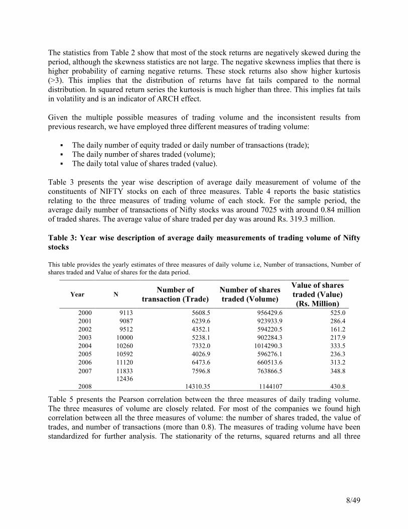
Table 3 presents the year wise description of average daily measurement of volume of the
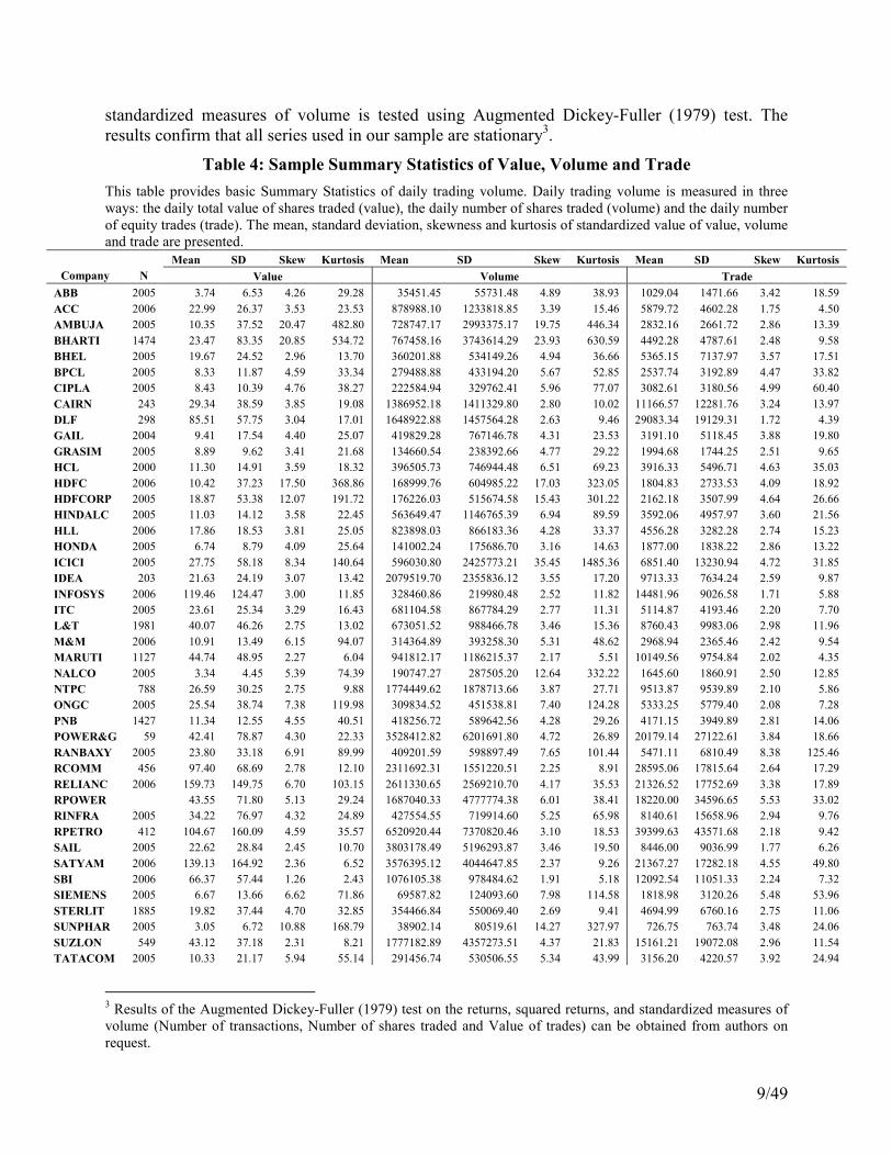
constituents of NIFTY stocks on each of three measures. Table 4 reports the basic statistics
relating to the three measures of trading volume of each stock. For the sample period, the
average daily number of transactions of Nifty stocks was around 7025 with around 0.84 million
of traded shares. The average value of share traded per day was around Rs. 319.3 million.
Table 3: Year wise description of average daily measurements of trading volume of Nifty
stocks
This table provides the yearly estimates of three measures of daily volume i.e, Number of transactions, Number of
shares traded and Value of shares for the data period.
Year N Number of
transaction (Trade)
Number of shares
traded (Volume)
Value of shares
traded (Value)
(Rs. Million) 2000 9113 5608.5 956429.6 525.0
2001 9087 6239.6 923933.9 286.4
2002 9512 4352.1 594220.5 161.2
2003 10000 5238.1 902284.3 217.9
2004 10260 7332.0 1014290.3 333.5
2005 10592 4026.9 596276.1 236.3
2006 11120 6473.6 660513.6 313.2
2007 11833 7596.8 763866.5 348.8
2008
12436
14310.35 1144107 430.8
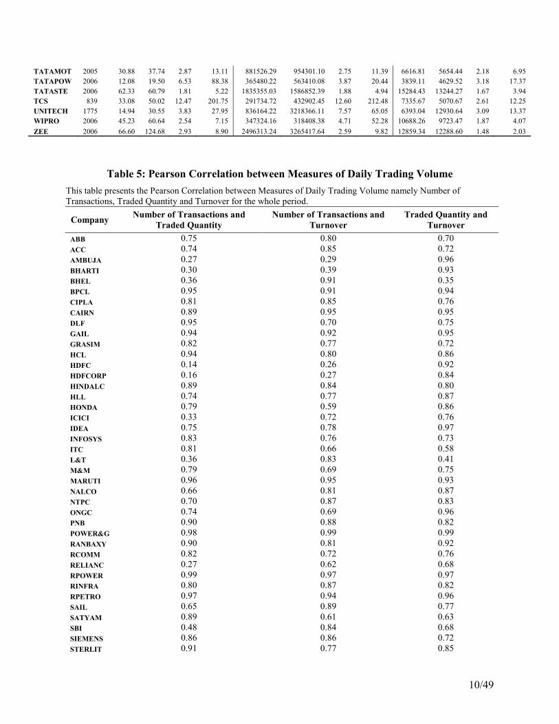
Table 5 presents the Pearson correlation between the three measures of daily trading volume.
The three measures of volume are closely related. For most of the companies we found high
correlation between all the three measures of volume: the number of shares traded, the value of
trades, and number of transactions (more than 0.8). The measures of trading volume have been
standardized for further analysis. The stationarity of the returns, squared returns and all three
9/49
standardized measures of volume is tested using Augmented Dickey-Fuller (1979) test. The
results confirm that all series used in our sample are stationary3.
Table 4: Sample Summary Statistics of Value, Volume and Trade
This table provides basic Summary Statistics of daily trading volume. Daily trading volume is measured in three
ways: the daily total value of shares traded (value), the daily number of shares traded (volume) and the daily number
of equity trades (trade). The mean, standard deviation, skewness and kurtosis of standardized value of value, volume
and trade are presented.
Mean SD Skew Kurtosis Mean SD Skew Kurtosis Mean SD Skew Kurtosis
Company N Value Volume Trade
ABB 2005 3.74 6.53 4.26 29.28 35451.45 55731.48 4.89 38.93 1029.04 1471.66 3.42 18.59
ACC 2006 22.99 26.37 3.53 23.53 878988.10 1233818.85 3.39 15.46 5879.72 4602.28 1.75 4.50
AMBUJA 2005 10.35 37.52 20.47 482.80 728747.17 2993375.17 19.75 446.34 2832.16 2661.72 2.86 13.39
BHARTI 1474 23.47 83.35 20.85 534.72 767458.16 3743614.29 23.93 630.59 4492.28 4787.61 2.48 9.58
BHEL 2005 19.67 24.52 2.96 13.70 360201.88 534149.26 4.94 36.66 5365.15 7137.97 3.57 17.51
BPCL 2005 8.33 11.87 4.59 33.34 279488.88 433194.20 5.67 52.85 2537.74 3192.89 4.47 33.82
CIPLA 2005 8.43 10.39 4.76 38.27 222584.94 329762.41 5.96 77.07 3082.61 3180.56 4.99 60.40
CAIRN 243 29.34 38.59 3.85 19.08 1386952.18 1411329.80 2.80 10.02 11166.57 12281.76 3.24 13.97
DLF 298 85.51 57.75 3.04 17.01 1648922.88 1457564.28 2.63 9.46 29083.34 19129.31 1.72 4.39
GAIL 2004 9.41 17.54 4.40 25.07 419829.28 767146.78 4.31 23.53 3191.10 5118.45 3.88 19.80
GRASIM 2005 8.89 9.62 3.41 21.68 134660.54 238392.66 4.77 29.22 1994.68 1744.25 2.51 9.65
HCL 2000 11.30 14.91 3.59 18.32 396505.73 746944.48 6.51 69.23 3916.33 5496.71 4.63 35.03
HDFC 2006 10.42 37.23 17.50 368.86 168999.76 604985.22 17.03 323.05 1804.83 2733.53 4.09 18.92
HDFCORP 2005 18.87 53.38 12.07 191.72 176226.03 515674.58 15.43 301.22 2162.18 3507.99 4.64 26.66
HINDALC 2005 11.03 14.12 3.58 22.45 563649.47 1146765.39 6.94 89.59 3592.06 4957.97 3.60 21.56
HLL 2006 17.86 18.53 3.81 25.05 823898.03 866183.36 4.28 33.37 4556.28 3282.28 2.74 15.23
HONDA 2005 6.74 8.79 4.09 25.64 141002.24 175686.70 3.16 14.63 1877.00 1838.22 2.86 13.22
ICICI 2005 27.75 58.18 8.34 140.64 596030.80 2425773.21 35.45 1485.36 6851.40 13230.94 4.72 31.85
IDEA 203 21.63 24.19 3.07 13.42 2079519.70 2355836.12 3.55 17.20 9713.33 7634.24 2.59 9.87
INFOSYS 2006 119.46 124.47 3.00 11.85 328460.86 219980.48 2.52 11.82 14481.96 9026.58 1.71 5.88
ITC 2005 23.61 25.34 3.29 16.43 681104.58 867784.29 2.77 11.31 5114.87 4193.46 2.20 7.70
L&T 1981 40.07 46.26 2.75 13.02 673051.52 988466.78 3.46 15.36 8760.43 9983.06 2.98 11.96
M&M 2006 10.91 13.49 6.15 94.07 314364.89 393258.30 5.31 48.62 2968.94 2365.46 2.42 9.54
MARUTI 1127 44.74 48.95 2.27 6.04 941812.17 1186215.37 2.17 5.51 10149.56 9754.84 2.02 4.35
NALCO 2005 3.34 4.45 5.39 74.39 190747.27 287505.20 12.64 332.22 1645.60 1860.91 2.50 12.85
NTPC 788 26.59 30.25 2.75 9.88 1774449.62 1878713.66 3.87 27.71 9513.87 9539.89 2.10 5.86
ONGC 2005 25.54 38.74 7.38 119.98 309834.52 451538.81 7.40 124.28 5333.25 5779.40 2.08 7.28
PNB 1427 11.34 12.55 4.55 40.51 418256.72 589642.56 4.28 29.26 4171.15 3949.89 2.81 14.06
POWER&G 59 42.41 78.87 4.30 22.33 3528412.82 6201691.80 4.72 26.89 20179.14 27122.61 3.84 18.66
RANBAXY 2005 23.80 33.18 6.91 89.99 409201.59 598897.49 7.65 101.44 5471.11 6810.49 8.38 125.46
RCOMM 456 97.40 68.69 2.78 12.10 2311692.31 1551220.51 2.25 8.91 28595.06 17815.64 2.64 17.29
RELIANC 2006 159.73 149.75 6.70 103.15 2611330.65 2569210.70 4.17 35.53 21326.52 17752.69 3.38 17.89
RPOWER 43.55 71.80 5.13 29.24 1687040.33 4777774.38 6.01 38.41 18220.00 34596.65 5.53 33.02
RINFRA 2005 34.22 76.97 4.32 24.89 427554.55 719914.60 5.25 65.98 8140.61 15658.96 2.94 9.76
RPETRO 412 104.67 160.09 4.59 35.57 6520920.44 7370820.46 3.10 18.53 39399.63 43571.68 2.18 9.42
SAIL 2005 22.62 28.84 2.45 10.70 3803178.49 5196293.87 3.46 19.50 8446.00 9036.99 1.77 6.26
SATYAM 2006 139.13 164.92 2.36 6.52 3576395.12 4044647.85 2.37 9.26 21367.27 17282.18 4.55 49.80
SBI 2006 66.37 57.44 1.26 2.43 1076105.38 978484.62 1.91 5.18 12092.54 11051.33 2.24 7.32
SIEMENS 2005 6.67 13.66 6.62 71.86 69587.82 124093.60 7.98 114.58 1818.98 3120.26 5.48 53.96
STERLIT 1885 19.82 37.44 4.70 32.85 354466.84 550069.40 2.69 9.41 4694.99 6760.16 2.75 11.06
SUNPHAR 2005 3.05 6.72 10.88 168.79 38902.14 80519.61 14.27 327.97 726.75 763.74 3.48 24.06
SUZLON 549 43.12 37.18 2.31 8.21 1777182.89 4357273.51 4.37 21.83 15161.21 19072.08 2.96 11.54
TATACOM 2005 10.33 21.17 5.94 55.14 291456.74 530506.55 5.34 43.99 3156.20 4220.57 3.92 24.94
3 Results of the Augmented Dickey-Fuller (1979) test on the returns, squared returns, and standardized measures of
volume (Number of transactions, Number of shares traded and Value of trades) can be obtained from authors on
request.
10/49
TATAMOT 2005 30.88 37.74 2.87 13.11 881526.29 954301.10 2.75 11.39 6616.81 5654.44 2.18 6.95
TATAPOW 2006 12.08 19.50 6.53 88.38 365480.22 563410.08 3.87 20.44 3839.11 4629.52 3.18 17.37
TATASTE 2006 62.33 60.79 1.81 5.22 1835355.03 1586852.39 1.88 4.94 15284.43 13244.27 1.67 3.94
TCS 839 33.08 50.02 12.47 201.75 291734.72 432902.45 12.60 212.48 7335.67 5070.67 2.61 12.25
UNITECH 1775 14.94 30.55 3.83 27.95 836164.22 3218366.11 7.57 65.05 6393.04 12930.64 3.09 13.37
WIPRO 2006 45.23 60.64 2.54 7.15 347324.16 318408.38 4.71 52.28 10688.26 9723.47 1.87 4.07
ZEE 2006 66.60 124.68 2.93 8.90 2496313.24 3265417.64 2.59 9.82 12859.34 12288.60 1.48 2.03
Table 5: Pearson Correlation between Measures of Daily Trading Volume
This table presents the Pearson Correlation between Measures of Daily Trading Volume namely Number of
Transactions, Traded Quantity and Turnover for the whole period.
Company Number of Transactions and
Traded Quantity
Number of Transactions and
Turnover
Traded Quantity and
Turnover
ABB 0.75 0.80 0.70
ACC 0.74 0.85 0.72
AMBUJA 0.27 0.29 0.96
BHARTI 0.30 0.39 0.93
BHEL 0.36 0.91 0.35
BPCL 0.95 0.91 0.94
CIPLA 0.81 0.85 0.76
CAIRN 0.89 0.95 0.95
DLF 0.95 0.70 0.75
GAIL 0.94 0.92 0.95
GRASIM 0.82 0.77 0.72
HCL 0.94 0.80 0.86
HDFC 0.14 0.26 0.92
HDFCORP 0.16 0.27 0.84
HINDALC 0.89 0.84 0.80
HLL 0.74 0.77 0.87
HONDA 0.79 0.59 0.86
ICICI 0.33 0.72 0.76
IDEA 0.75 0.78 0.97
INFOSYS 0.83 0.76 0.73
ITC 0.81 0.66 0.58
L&T 0.36 0.83 0.41
M&M 0.79 0.69 0.75
MARUTI 0.96 0.95 0.93
NALCO 0.66 0.81 0.87
NTPC 0.70 0.87 0.83
ONGC 0.74 0.69 0.96
PNB 0.90 0.88 0.82
POWER&G 0.98 0.99 0.99
RANBAXY 0.90 0.81 0.92
RCOMM 0.82 0.72 0.76
RELIANC 0.27 0.62 0.68
RPOWER 0.99 0.97 0.97
RINFRA 0.80 0.87 0.82
RPETRO 0.97 0.94 0.96
SAIL 0.65 0.89 0.77
SATYAM 0.89 0.61 0.63
SBI 0.48 0.84 0.68
SIEMENS 0.86 0.86 0.72
STERLIT 0.91 0.77 0.85
11/49
SUNPHAR 0.39 0.39 0.89
SUZLON 0.91 0.70 0.56
TATACOM 0.91 0.89 0.97
TATAMOT 0.82 0.89 0.77
TATAPOW 0.81 0.88 0.71
TATASTE 0.70 0.79 0.84
TCS 0.43 0.37 0.97
UNITECH 0.80 0.81 0.54
WIPRO 0.75 0.85 0.73
ZEE 0.92 0.78 0.75
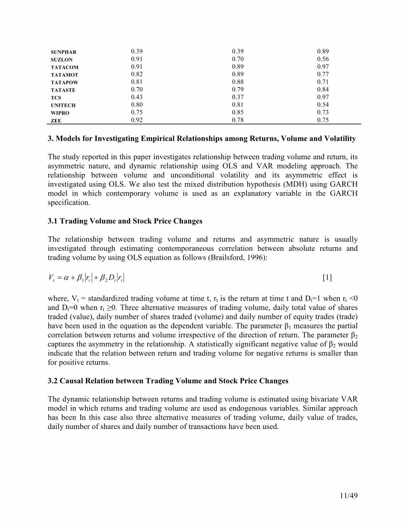
3. Models for Investigating Empirical Relationships among Returns, Volume and Volatility
The study reported in this paper investigates relationship between trading volume and return, its
asymmetric nature, and dynamic relationship using OLS and VAR modeling approach. The
relationship between volume and unconditional volatility and its asymmetric effect is
investigated using OLS. We also test the mixed distribution hypothesis (MDH) using GARCH
model in which contemporary volume is used as an explanatory variable in the GARCH
specification.
3.1 Trading Volume and Stock Price Changes
The relationship between trading volume and returns and asymmetric nature is usually
investigated through estimating contemporaneous correlation between absolute returns and
trading volume by using OLS equation as follows (Brailsford, 1996):
tttt rDrV 21 ββα ++= [1]
where, Vt = standardized trading volume at time t, rt is the return at time t and Dt=1 when rt <0
and Dt=0 when rt ≥0. Three alternative measures of trading volume, daily total value of shares
traded (value), daily number of shares traded (volume) and daily number of equity trades (trade)
have been used in the equation as the dependent variable. The parameter β1 measures the partial
correlation between returns and volume irrespective of the direction of return. The parameter β2
captures the asymmetry in the relationship. A statistically significant negative value of β2 would
indicate that the relation between return and trading volume for negative returns is smaller than
for positive returns.
3.2 Causal Relation between Trading Volume and Stock Price Changes
The dynamic relationship between returns and trading volume is estimated using bivariate VAR
model in which returns and trading volume are used as endogenous variables. Similar approach
has been In this case also three alternative measures of trading volume, daily value of trades,
daily number of shares and daily number of transactions have been used.
12/49
∑∑
∑∑
=−
=−
=−
=−
++=
++=
5
1
5
1
0
5
1
5
1
0
j
jtj
i
itit
j
jtj
i
itit
rVV
Vrr
δγγ
βαα
[2]
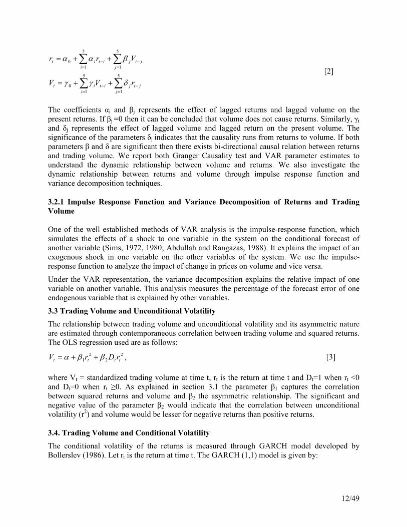
The coefficients αi and βj represents the effect of lagged returns and lagged volume on the
present returns. If βj =0 then it can be concluded that volume does not cause returns. Similarly, γi
and δj represents the effect of lagged volume and lagged return on the present volume. The
significance of the parameters δj indicates that the causality runs from returns to volume. If both
parameters β and δ are significant then there exists bi-directional causal relation between returns
and trading volume. We report both Granger Causality test and VAR parameter estimates to
understand the dynamic relationship between volume and returns. We also investigate the
dynamic relationship between returns and volume through impulse response function and
variance decomposition techniques.
3.2.1 Impulse Response Function and Variance Decomposition of Returns and Trading
Volume
One of the well established methods of VAR analysis is the impulse-response function, which
simulates the effects of a shock to one variable in the system on the conditional forecast of
another variable (Sims, 1972, 1980; Abdullah and Rangazas, 1988). It explains the impact of an
exogenous shock in one variable on the other variables of the system. We use the impulse-
response function to analyze the impact of change in prices on volume and vice versa.
Under the VAR representation, the variance decomposition explains the relative impact of one
variable on another variable. This analysis measures the percentage of the forecast error of one
endogenous variable that is explained by other variables.
3.3 Trading Volume and Unconditional Volatility
The relationship between trading volume and unconditional volatility and its asymmetric nature
are estimated through contemporaneous correlation between trading volume and squared returns.
The OLS regression used are as follows:
2
2
2
1 tttt rDrV ββα ++= , [3]
where Vt = standardized trading volume at time t, rt is the return at time t and Dt=1 when rt <0
and Dt=0 when rt ≥0. As explained in section 3.1 the parameter β1 captures the correlation
between squared returns and volume and β2 the asymmetric relationship. The significant and
negative value of the parameter β2 would indicate that the correlation between unconditional
volatility (r2) and volume would be lesser for negative returns than positive returns.
3.4. Trading Volume and Conditional Volatility
The conditional volatility of the returns is measured through GARCH model developed by
Bollerslev (1986). Let rt is the return at time t. The GARCH (1,1) model is given by:
13/49
t
i
itit rbar ε++= ∑=
−
5
1
),0(~| 2
1 ttt N σψε − and [4]
∑∑=
−=
− ++=p
j
jtJ
q
i
itit
1
2
1
2
0
2 σβεαασ .
The parameters α and β measure the dependence of present volatility ( 2σ ) on innovation term
( it−ε ) and past volatility ( jt−σ ) respectively. The persistence of the conditional volatility is
measured by α+β. The relationship between conditional volatility and trading volume is modeled
by modifying GARCH equation. The contemporaneous volume is used as explanatory variable
in GARCH equation (Lamoureux and Lastrapes, 1990) as follows:
t
i
itit rbar ε++= ∑=
−
5
1
),0(~| 2
1 ttt N σψε − and [5]
t
p
j
jtJ
q
i
itit Vχσβεαασ +++= ∑∑=
−=
−1
2
1
2
0
2.
The significance of the coefficient estimate ( χ ) of volume indicates the influence of trading
volume on the conditional volatility.
4. Results and Discussions on Relationship between Volume, Returns and Volatility
In this section of the paper we present empirical results on the relationship between trading
volume, returns and volatility (conditional and unconditional). Firstly we report the relationship
between trading volume and price changes. Later, we report the relationship between volume and
unconditional and conditional volatility.
4.1 Trading Volume and Stock Price Changes
The results of the OLS regression using equation [1] to explain the relation between volume and
price changes and its asymmetric nature are presented in Table 6. The estimates of β1, which
measure the relationship between price changes and volume irrespective of the direction of the
price change, are significant and positive at 1% level (except for Idea Cellular Ltd., where the
coefficient is significant at 5% level and Reliance Power, where it is not significant) across all
three measures of trading volume. The coefficients are higher for most of the companies, when
the number of transactions is taken as a measure of trading volume.
The asymmetric behavior of relation between volume and returns is indicated by coefficient β2. In most of the cases, β2 is significant and negative i.e. for most stocks β2 is negative for at least
two out of the three trading volume measures. The negative value of β2 indicates that the relation
between price changes and trading volume is smaller for negative returns than for positive
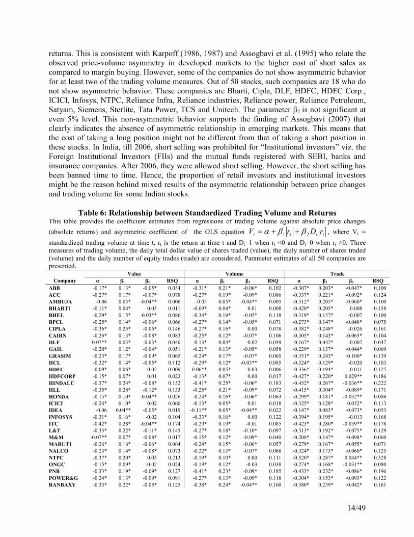
14/49
returns. This is consistent with Karpoff (1986, 1987) and Assogbavi et al. (1995) who relate the
observed price-volume asymmetry in developed markets to the higher cost of short sales as
compared to margin buying. However, some of the companies do not show asymmetric behavior
for at least two of the trading volume measures. Out of 50 stocks, such companies are 18 who do
not show asymmetric behavior. These companies are Bharti, Cipla, DLF, HDFC, HDFC Corp.,
ICICI, Infosys, NTPC, Reliance Infra, Reliance industries, Reliance power, Reliance Petroleum,
Satyam, Siemens, Sterlite, Tata Power, TCS and Unitech. The parameter β2 is not significant at
even 5% level. This non-asymmetric behavior supports the finding of Assogbavi (2007) that
clearly indicates the absence of asymmetric relationship in emerging markets. This means that
the cost of taking a long position might not be different from that of taking a short position in
these stocks. In India, till 2006, short selling was prohibited for “Institutional investors” viz. the
Foreign Institutional Investors (FIIs) and the mutual funds registered with SEBI, banks and
insurance companies. After 2006, they were allowed short selling. However, the short selling has
been banned time to time. Hence, the proportion of retail investors and institutional investors
might be the reason behind mixed results of the asymmetric relationship between price changes
and trading volume for some Indian stocks.
Table 6: Relationship between Standardized Trading Volume and Returns This table provides the coefficient estimates from regressions of trading volume against absolute price changes
(absolute returns) and asymmetric coefficient of the OLS equation tttt rDrV 21 ββα ++= , where Vt =
standardized trading volume at time t, rt is the return at time t and Dt=1 when rt <0 and Dt=0 when rt ≥0. Three
measures of trading volume, the daily total dollar value of shares traded (value), the daily number of shares traded
(volume) and the daily number of equity trades (trade) are considered. Parameter estimates of all 50 companies are
presented. Value Volume Trade
Company α β1 β2 RSQ α β1 β2 RSQ α β1 β2 RSQ
ABB -0.17* 0.13* -0.05* 0.034 -0.31* 0.21* -0.06* 0.102 -0.307* 0.203* -0.047* 0.100
ACC -0.27* 0.17* -0.07* 0.078 -0.27* 0.19* -0.09* 0.086 -0.337* 0.221* -0.092* 0.124
AMBUJA -0.06 0.05* -0.04** 0.006 -0.05 0.05* -0.04** 0.005 -0.312* 0.205* -0.060* 0.100
BHARTI -0.11* 0.04* 0.03 0.011 -0.09* 0.04* 0.01 0.008 -0.420* 0.205* 0.008 0.158
BHEL -0.29* 0.15* -0.03** 0.086 -0.34* 0.19* -0.05* 0.118 -0.319* 0.157* -0.007 0.100
BPCL -0.25* 0.14* -0.06* 0.066 -0.27* 0.14* -0.05* 0.071 -0.273* 0.147* -0.048* 0.075
CIPLA -0.36* 0.25* -0.06* 0.146 -0.27* 0.16* 0.00 0.078 -0.382* 0.248* -0.026 0.161
CAIRN -0.26* 0.13* -0.08* 0.083 -0.25* 0.12* -0.07* 0.106 -0.305* 0.143* -0.065* 0.104
DLF -0.07** 0.03* -0.03* 0.040 -0.13* 0.04* -0.02 0.049 -0.167* 0.042* -0.002 0.047
GAIL -0.20* 0.12* -0.04* 0.051 -0.21* 0.13* -0.05* 0.058 -0.229* 0.137* -0.044* 0.069
GRASIM -0.23* 0.17* -0.09* 0.065 -0.24* 0.17* -0.07* 0.065 -0.351* 0.243* -0.100* 0.139
HCL -0.32* 0.14* -0.05* 0.112 -0.29* 0.12* -0.03** 0.085 -0.324* 0.129* -0.020 0.103
HDFC -0.09* 0.06* -0.02 0.009 -0.06** 0.05* -0.03 0.006 -0.336* 0.194* 0.011 0.125
HDFCORP -0.15* 0.07* 0.01 0.022 -0.13* 0.07* 0.00 0.017 -0.427* 0.220* 0.029** 0.186
HINDALC -0.37* 0.24* -0.08* 0.152 -0.41* 0.25* -0.06* 0.183 -0.452* 0.267* -0.036** 0.222
HLL -0.35* 0.28* -0.12* 0.133 -0.25* 0.21* -0.09* 0.072 -0.415* 0.304* -0.089* 0.171
HONDA -0.15* 0.10* -0.04** 0.026 -0.24* 0.16* -0.06* 0.063 -0.299* 0.181* -0.032** 0.086
ICICI -0.24* 0.10* 0.02 0.060 -0.13* 0.05* 0.01 0.018 -0.325* 0.128* 0.032* 0.113
IDEA -0.06 0.04** -0.05* 0.019 -0.11** 0.05* -0.04** 0.022 -0.147* 0.083* -0.073* 0.053
INFOSYS -0.31* 0.16* -0.02 0.104 -0.33* 0.16* 0.00 0.122 -0.394* 0.195* -0.013 0.168
ITC -0.42* 0.28* -0.04** 0.174 -0.29* 0.19* -0.01 0.085 -0.423* 0.280* -0.039** 0.178
L&T -0.33* 0.22* -0.11* 0.145 -0.27* 0.18* -0.10* 0.097 -0.313* 0.192* -0.075* 0.129
M&M -0.07** 0.07* -0.08* 0.017 -0.15* 0.12* -0.09* 0.040 -0.208* 0.147* -0.098* 0.060
MARUTI -0.26* 0.16* -0.06* 0.064 -0.24* 0.15* -0.06* 0.057 -0.279* 0.167* -0.055* 0.071
NALCO -0.23* 0.14* -0.08* 0.073 -0.22* 0.13* -0.07* 0.068 -0.324* 0.173* -0.060* 0.125
NTPC -0.37* 0.20* 0.03 0.213 -0.19* 0.10* 0.00 0.111 -0.520* 0.287* 0.044** 0.328
ONGC -0.15* 0.09* -0.02 0.024 -0.19* 0.12* -0.03 0.038 -0.274* 0.168* -0.031** 0.080
PNB -0.33* 0.19* -0.09* 0.127 -0.41* 0.23* -0.09* 0.185 -0.433* 0.232* -0.086* 0.196
POWER&G -0.24* 0.13* -0.09* 0.091 -0.27* 0.13* -0.09* 0.118 -0.304* 0.153* -0.093* 0.122
RANBAXY -0.33* 0.22* -0.05* 0.125 -0.38* 0.24* -0.04** 0.160 -0.380* 0.239* -0.042* 0.161
15/49
RCOMM -0.24* 0.11* -0.04** 0.064 -0.38* 0.16* -0.04** 0.175 -0.459* 0.194* -0.038** 0.229
RELIANC -0.35* 0.20* 0.01 0.140 -0.33* 0.21* -0.04* 0.119 -0.445* 0.244* 0.019 0.223
RPOWER -0.04* 0.00* 0.02* 0.002 -0.05 0.00 0.02 0.004 -0.060 0.009 0.019 0.004
RINFRA -0.33* 0.18* -0.04* 0.152 -0.40* 0.22* -0.06* 0.227 -0.372* 0.188* -0.023 0.190
RPETRO -0.40* 0.21* -0.03 0.211 -0.48* 0.25* -0.04** 0.325 -0.465* 0.235* -0.026 0.281
SAIL -0.26* 0.12* -0.04* 0.083 -0.31* 0.15* -0.05* 0.116 -0.314* 0.134* -0.020 0.111
SATYAM -0.34* 0.14* -0.02 0.116 -0.33* 0.13* -0.01 0.107 -0.409* 0.157* 0.000 0.164
SBI -0.32* 0.20* -0.04** 0.096 -0.32* 0.20* -0.06* 0.097 -0.361* 0.208* -0.024 0.118
SIEMENS -0.25* 0.15* -0.03 0.072 -0.35* 0.17* 0.04** 0.141 -0.330* 0.167* 0.023 0.120
STERLIT -0.17* 0.10* -0.08* 0.063 -0.20* 0.11* -0.07* 0.096 -0.175* 0.097* -0.065* 0.070
SUNPHAR -0.13* 0.09* -0.03 0.020 -0.13* 0.09* -0.04* 0.022 -0.371* 0.234* -0.056* 0.158
SUZLON -0.33* 0.14* -0.07* 0.202 -0.37* 0.15* -0.04* 0.162 -0.452* 0.171* -0.040* 0.257
TATACOM -0.14* 0.09* -0.07* 0.038 -0.15* 0.10* -0.07* 0.040 -0.177* 0.108* -0.068* 0.051
TATAMOT -0.08* 0.06* -0.04* 0.009 -0.24* 0.15* -0.08* 0.059 -0.205* 0.119* -0.046* 0.039
TATAPOW -0.33* 0.17* -0.02 0.123 -0.29* 0.16* -0.04* 0.093 -0.335* 0.171* -0.016 0.124
TATASTE -0.26* 0.14* -0.04* 0.066 -0.30* 0.17* -0.06* 0.091 -0.396* 0.196* -0.019 0.149
TCS -0.10** 0.06* -0.02 0.009 -0.16* 0.10* -0.02 0.025 -0.376* 0.212* 0.007 0.190
UNITECH -0.21* 0.08* -0.03* 0.049 -0.30* 0.10* -0.01 0.092 -0.294* 0.094* -0.004 0.089
WIPRO -0.27* 0.13* -0.03* 0.085 -0.25* 0.12* -0.03* 0.072 -0.320* 0.142* -0.023** 0.117
ZEE -0.26* 0.11* -0.03** 0.066 -0.32* 0.14* -0.05* 0.105 -0.360* 0.155* -0.049* 0.134
*(**) represents significance of the parameter at 1 %( 5%) significance level.
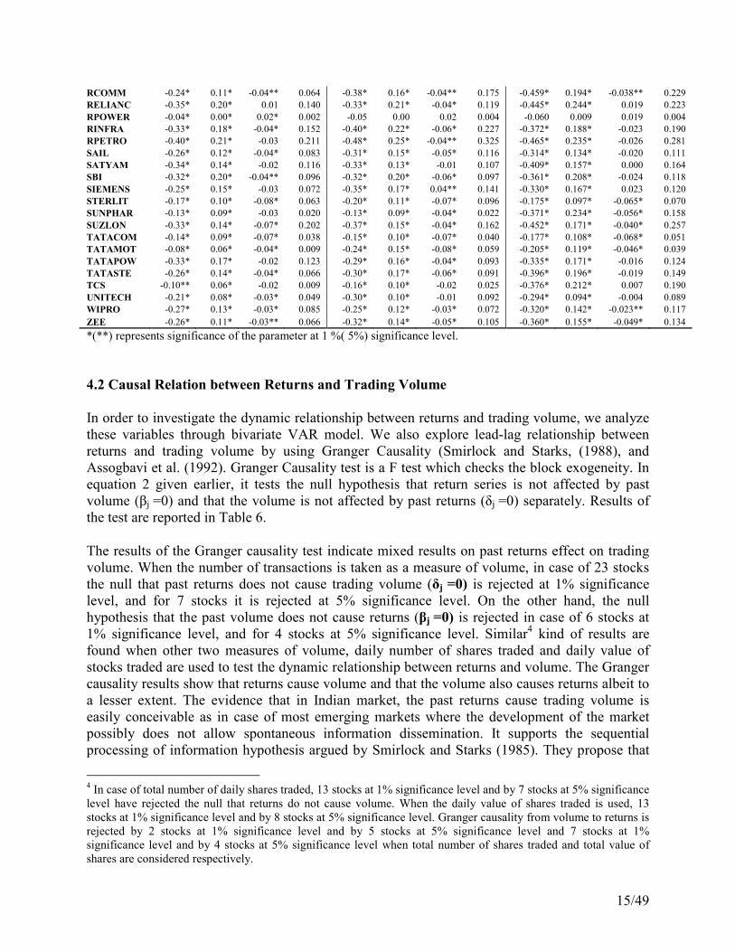
4.2 Causal Relation between Returns and Trading Volume
In order to investigate the dynamic relationship between returns and trading volume, we analyze
these variables through bivariate VAR model. We also explore lead-lag relationship between
returns and trading volume by using Granger Causality (Smirlock and Starks, (1988), and
Assogbavi et al. (1992). Granger Causality test is a F test which checks the block exogeneity. In
equation 2 given earlier, it tests the null hypothesis that return series is not affected by past
volume (βj =0) and that the volume is not affected by past returns (δj =0) separately. Results of
the test are reported in Table 6.
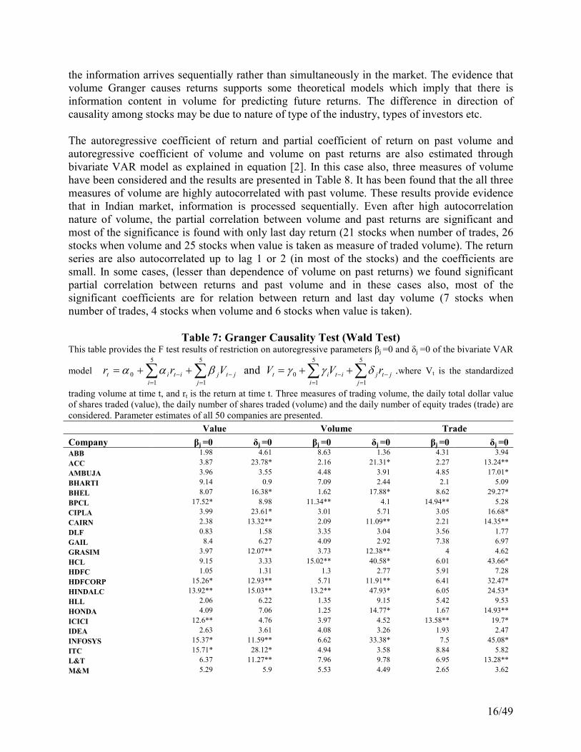
The results of the Granger causality test indicate mixed results on past returns effect on trading
volume. When the number of transactions is taken as a measure of volume, in case of 23 stocks
the null that past returns does not cause trading volume (δj =0) is rejected at 1% significance
level, and for 7 stocks it is rejected at 5% significance level. On the other hand, the null
hypothesis that the past volume does not cause returns (βj =0) is rejected in case of 6 stocks at
1% significance level, and for 4 stocks at 5% significance level. Similar4 kind of results are
found when other two measures of volume, daily number of shares traded and daily value of
stocks traded are used to test the dynamic relationship between returns and volume. The Granger
causality results show that returns cause volume and that the volume also causes returns albeit to
a lesser extent. The evidence that in Indian market, the past returns cause trading volume is
easily conceivable as in case of most emerging markets where the development of the market
possibly does not allow spontaneous information dissemination. It supports the sequential
processing of information hypothesis argued by Smirlock and Starks (1985). They propose that
4 In case of total number of daily shares traded, 13 stocks at 1% significance level and by 7 stocks at 5% significance
level have rejected the null that returns do not cause volume. When the daily value of shares traded is used, 13
stocks at 1% significance level and by 8 stocks at 5% significance level. Granger causality from volume to returns is
rejected by 2 stocks at 1% significance level and by 5 stocks at 5% significance level and 7 stocks at 1%
significance level and by 4 stocks at 5% significance level when total number of shares traded and total value of
shares are considered respectively.
16/49
the information arrives sequentially rather than simultaneously in the market. The evidence that
volume Granger causes returns supports some theoretical models which imply that there is
information content in volume for predicting future returns. The difference in direction of
causality among stocks may be due to nature of type of the industry, types of investors etc.
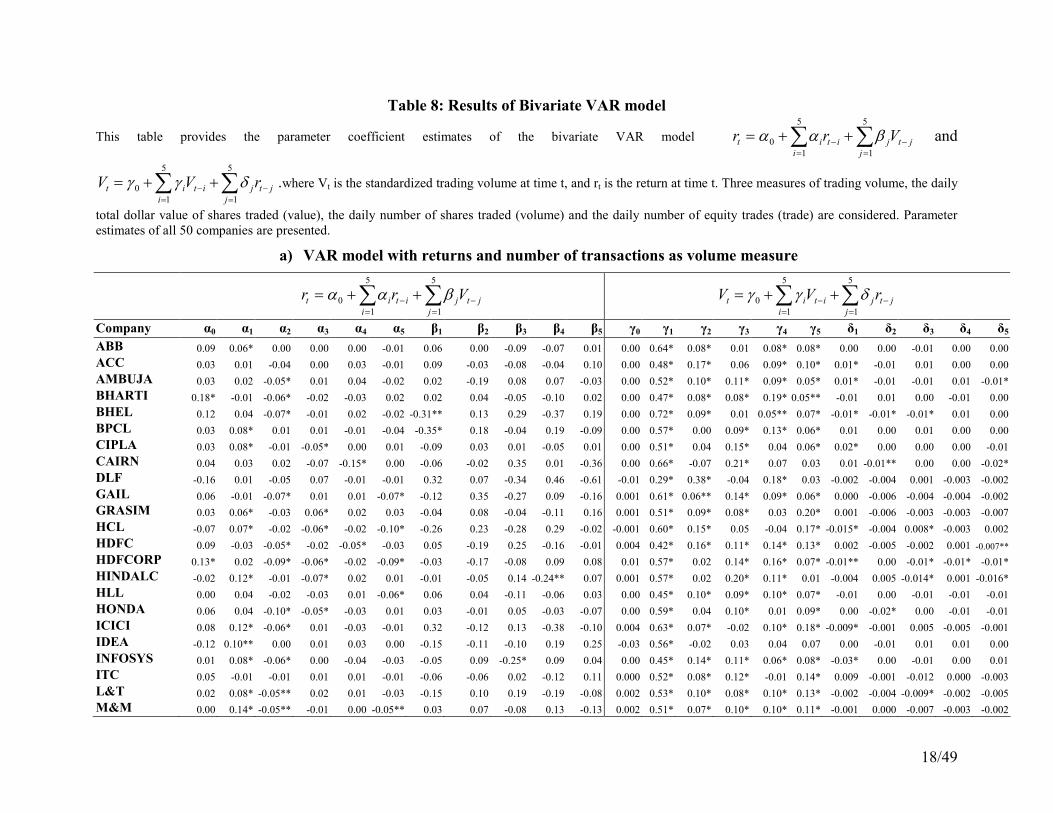
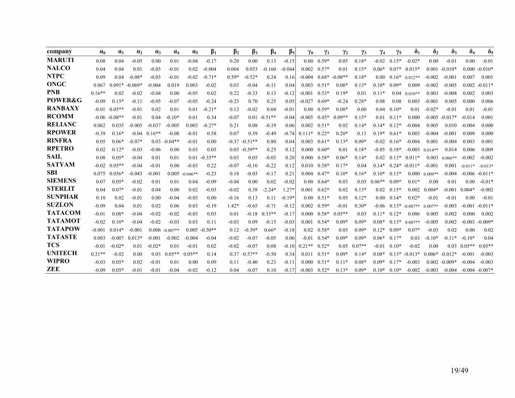
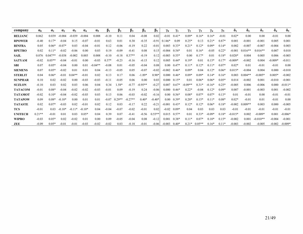
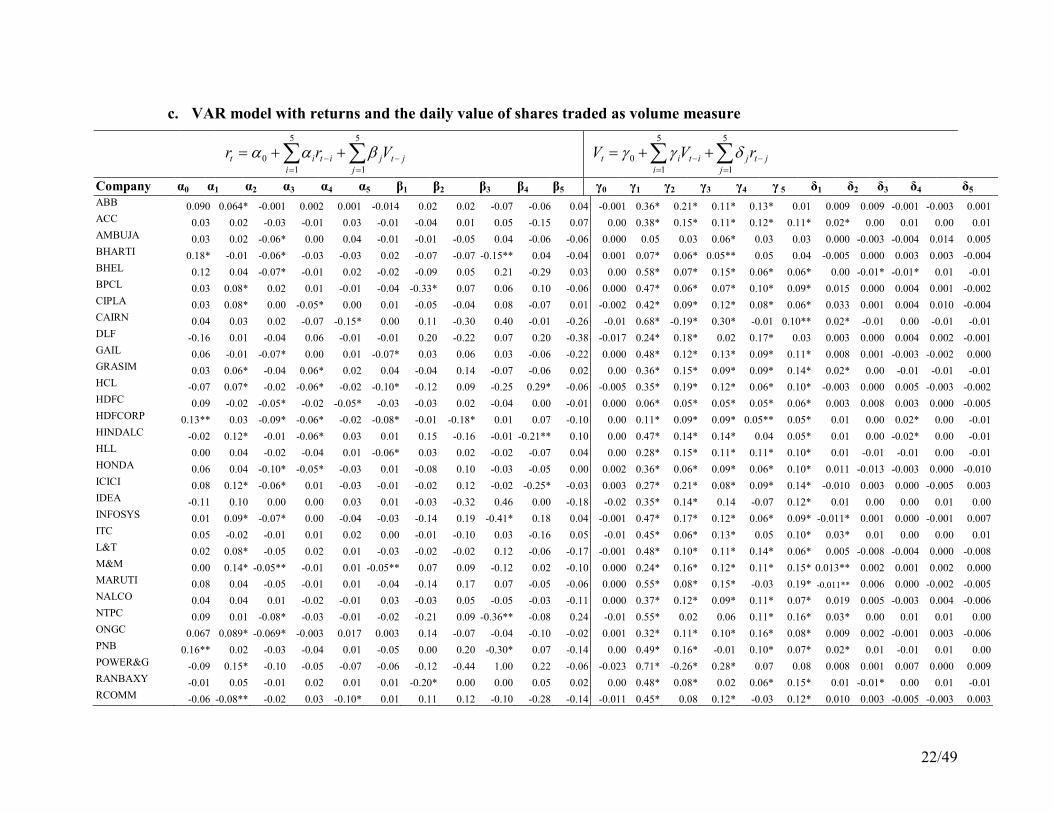
The autoregressive coefficient of return and partial coefficient of return on past volume and
autoregressive coefficient of volume and volume on past returns are also estimated through
bivariate VAR model as explained in equation [2]. In this case also, three measures of volume
have been considered and the results are presented in Table 8. It has been found that the all three
measures of volume are highly autocorrelated with past volume. These results provide evidence
that in Indian market, information is processed sequentially. Even after high autocorrelation
nature of volume, the partial correlation between volume and past returns are significant and
most of the significance is found with only last day return (21 stocks when number of trades, 26
stocks when volume and 25 stocks when value is taken as measure of traded volume). The return
series are also autocorrelated up to lag 1 or 2 (in most of the stocks) and the coefficients are
small. In some cases, (lesser than dependence of volume on past returns) we found significant
partial correlation between returns and past volume and in these cases also, most of the
significant coefficients are for relation between return and last day volume (7 stocks when
number of trades, 4 stocks when volume and 6 stocks when value is taken).
Table 7: Granger Causality Test (Wald Test) This table provides the F test results of restriction on autoregressive parameters βj =0 and δj =0 of the bivariate VAR
model ∑∑=
−=
− ++=5
1
5
1
0
j
jtj
i
itit Vrr βαα and ∑∑=
−=
− ++=5
1
5
1
0
j
jtj
i
itit rVV δγγ .where Vt is the standardized
trading volume at time t, and rt is the return at time t. Three measures of trading volume, the daily total dollar value
of shares traded (value), the daily number of shares traded (volume) and the daily number of equity trades (trade) are
considered. Parameter estimates of all 50 companies are presented.
Value Volume Trade
Company βj =0 δj =0 βj =0 δj =0 βj =0 δj =0
ABB 1.98 4.61 8.63 1.36 4.31 3.94
ACC 3.87 23.78* 2.16 21.31* 2.27 13.24**
AMBUJA 3.96 3.55 4.48 3.91 4.85 17.01*
BHARTI 9.14 0.9 7.09 2.44 2.1 5.09
BHEL 8.07 16.38* 1.62 17.88* 8.62 29.27*
BPCL 17.52* 8.98 11.34** 4.1 14.94** 5.28
CIPLA 3.99 23.61* 3.01 5.71 3.05 16.68*
CAIRN 2.38 13.32** 2.09 11.09** 2.21 14.35**
DLF 0.83 1.58 3.35 3.04 3.56 1.77
GAIL 8.4 6.27 4.09 2.92 7.38 6.97
GRASIM 3.97 12.07** 3.73 12.38** 4 4.62
HCL 9.15 3.33 15.02** 40.58* 6.01 43.66*
HDFC 1.05 1.31 1.3 2.77 5.91 7.28
HDFCORP 15.26* 12.93** 5.71 11.91** 6.41 32.47*
HINDALC 13.92** 15.03** 13.2** 47.93* 6.05 24.53*
HLL 2.06 6.22 1.35 9.15 5.42 9.53
HONDA 4.09 7.06 1.25 14.77* 1.67 14.93**
ICICI 12.6** 4.76 3.97 4.52 13.58** 19.7*
IDEA 2.63 3.61 4.08 3.26 1.93 2.47
INFOSYS 15.37* 11.59** 6.62 33.38* 7.5 45.08*
ITC 15.71* 28.12* 4.94 3.58 8.84 5.82
L&T 6.37 11.27** 7.96 9.78 6.95 13.28**
M&M 5.29 5.9 5.53 4.49 2.65 3.62

17/49
MARUTI 2.01 7.24 2.15 17.61* 2.35 23.39*
NALCO 5.28 17.01* 1.74 11.58** 5.18 24.06*
NTPC 16.76* 20.98* 5.4 7.15 29.9* 5.44
ONGC 8.18 3.07 5.88 2.74 3.89 11.05
PNB 11.33 12.6 14.99** 10.94 6.71 7.82
POWER&G 8.85 5.32 9.95 2.69 6.87 1.92
RANBAXY 10.42 10.9 7.68 13.8** 7.98 24.68*
RCOMM 6.16 2.31 5.88 5.7 10.64 8.57
RELIANC 8.19 12.04** 4.03 9.19 14.37** 7.91
RPOWER 7.36 0.49 6.22 0.27 6.48 0.9
RINFRA 14.34** 4.37 7 7.38 17.72* 8.07
RPETRO 7.38 23.75* 4.75 13.79** 5.9 13.63**
SAIL 8.14 43.76* 6.1 48.39* 7.6 20.42*
SATYAM 10.16 33.63* 8.52 39.95* 6.43 39.27*
SBI 4.59 21.39* 2.85 17.14* 7.88 17.91*
SIEMENS 5.82 8.65 11.55** 9.6 5.02 15.75*
STERLIT 190.34 78.76 67.15 20.33 63* 17.96*
SUNPHAR 12.59** 6.5 6.53 4.58 12.54** 22.57*
SUZLON 8.61 7.07 27.91* 21.39* 20.81* 18.29*
TATACOM 5.7 5.47 5.63 4.19 5.07 5.18
TATAMOT 0.84 11.11** 4.63 17.94* 2.11 13.8**
TATAPOW 40.51* 79.04* 22.31* 37.94* 25.21* 24.31*
TATASTE 6.12 17.55* 7.44 6.96 3 20.87*
TCS 0.67 0.11 1.24 2.57 1.57 19.06*
UNITECH 5.44 10.73 10.49 92.56* 16.82* 77.95*
WIPRO 10.9 8.91 2.43 6.44 5.16 21.26*
ZEE 15.19* 15.39* 7.61 14.51** 6.89 12.95**
18/49
Table 8: Results of Bivariate VAR model
This table provides the parameter coefficient estimates of the bivariate VAR model ∑∑=
−=
− ++=5
1
5
1
0
j
jtj
i
itit Vrr βαα and
∑∑=
−=
− ++=5
1
5
1
0
j
jtj
i
itit rVV δγγ .where Vt is the standardized trading volume at time t, and rt is the return at time t. Three measures of trading volume, the daily
total dollar value of shares traded (value), the daily number of shares traded (volume) and the daily number of equity trades (trade) are considered. Parameter
estimates of all 50 companies are presented.
a) VAR model with returns and number of transactions as volume measure
∑∑=
−=
− ++=5
1
5
1
0
j
jtj
i
itit Vrr βαα ∑∑=
−=
− ++=5
1
5
1
0
j
jtj
i
itit rVV δγγ
Company α0 α1 α2 α3 α4 α5 β1 β2 β3 β4 β5 γ0 γ1 γ2 γ3 γ4 γ5 δ1 δ2 δ3 δ4 δ5
ABB 0.09 0.06* 0.00 0.00 0.00 -0.01 0.06 0.00 -0.09 -0.07 0.01 0.00 0.64* 0.08* 0.01 0.08* 0.08* 0.00 0.00 -0.01 0.00 0.00
ACC 0.03 0.01 -0.04 0.00 0.03 -0.01 0.09 -0.03 -0.08 -0.04 0.10 0.00 0.48* 0.17* 0.06 0.09* 0.10* 0.01* -0.01 0.01 0.00 0.00
AMBUJA 0.03 0.02 -0.05* 0.01 0.04 -0.02 0.02 -0.19 0.08 0.07 -0.03 0.00 0.52* 0.10* 0.11* 0.09* 0.05* 0.01* -0.01 -0.01 0.01 -0.01*
BHARTI 0.18* -0.01 -0.06* -0.02 -0.03 0.02 0.02 0.04 -0.05 -0.10 0.02 0.00 0.47* 0.08* 0.08* 0.19* 0.05** -0.01 0.01 0.00 -0.01 0.00
BHEL 0.12 0.04 -0.07* -0.01 0.02 -0.02 -0.31** 0.13 0.29 -0.37 0.19 0.00 0.72* 0.09* 0.01 0.05** 0.07* -0.01* -0.01* -0.01* 0.01 0.00
BPCL 0.03 0.08* 0.01 0.01 -0.01 -0.04 -0.35* 0.18 -0.04 0.19 -0.09 0.00 0.57* 0.00 0.09* 0.13* 0.06* 0.01 0.00 0.01 0.00 0.00
CIPLA 0.03 0.08* -0.01 -0.05* 0.00 0.01 -0.09 0.03 0.01 -0.05 0.01 0.00 0.51* 0.04 0.15* 0.04 0.06* 0.02* 0.00 0.00 0.00 -0.01
CAIRN 0.04 0.03 0.02 -0.07 -0.15* 0.00 -0.06 -0.02 0.35 0.01 -0.36 0.00 0.66* -0.07 0.21* 0.07 0.03 0.01 -0.01** 0.00 0.00 -0.02*
DLF -0.16 0.01 -0.05 0.07 -0.01 -0.01 0.32 0.07 -0.34 0.46 -0.61 -0.01 0.29* 0.38* -0.04 0.18* 0.03 -0.002 -0.004 0.001 -0.003 -0.002
GAIL 0.06 -0.01 -0.07* 0.01 0.01 -0.07* -0.12 0.35 -0.27 0.09 -0.16 0.001 0.61* 0.06** 0.14* 0.09* 0.06* 0.000 -0.006 -0.004 -0.004 -0.002
GRASIM 0.03 0.06* -0.03 0.06* 0.02 0.03 -0.04 0.08 -0.04 -0.11 0.16 0.001 0.51* 0.09* 0.08* 0.03 0.20* 0.001 -0.006 -0.003 -0.003 -0.007
HCL -0.07 0.07* -0.02 -0.06* -0.02 -0.10* -0.26 0.23 -0.28 0.29 -0.02 -0.001 0.60* 0.15* 0.05 -0.04 0.17* -0.015* -0.004 0.008* -0.003 0.002
HDFC 0.09 -0.03 -0.05* -0.02 -0.05* -0.03 0.05 -0.19 0.25 -0.16 -0.01 0.004 0.42* 0.16* 0.11* 0.14* 0.13* 0.002 -0.005 -0.002 0.001 -0.007**
HDFCORP 0.13* 0.02 -0.09* -0.06* -0.02 -0.09* -0.03 -0.17 -0.08 0.09 0.08 0.01 0.57* 0.02 0.14* 0.16* 0.07* -0.01** 0.00 -0.01* -0.01* -0.01*
HINDALC -0.02 0.12* -0.01 -0.07* 0.02 0.01 -0.01 -0.05 0.14 -0.24** 0.07 0.001 0.57* 0.02 0.20* 0.11* 0.01 -0.004 0.005 -0.014* 0.001 -0.016*
HLL 0.00 0.04 -0.02 -0.03 0.01 -0.06* 0.06 0.04 -0.11 -0.06 0.03 0.00 0.45* 0.10* 0.09* 0.10* 0.07* -0.01 0.00 -0.01 -0.01 -0.01
HONDA 0.06 0.04 -0.10* -0.05* -0.03 0.01 0.03 -0.01 0.05 -0.03 -0.07 0.00 0.59* 0.04 0.10* 0.01 0.09* 0.00 -0.02* 0.00 -0.01 -0.01
ICICI 0.08 0.12* -0.06* 0.01 -0.03 -0.01 0.32 -0.12 0.13 -0.38 -0.10 0.004 0.63* 0.07* -0.02 0.10* 0.18* -0.009* -0.001 0.005 -0.005 -0.001
IDEA -0.12 0.10** 0.00 0.01 0.03 0.00 -0.15 -0.11 -0.10 0.19 0.25 -0.03 0.56* -0.02 0.03 0.04 0.07 0.00 -0.01 0.01 0.01 0.00
INFOSYS 0.01 0.08* -0.06* 0.00 -0.04 -0.03 -0.05 0.09 -0.25* 0.09 0.04 0.00 0.45* 0.14* 0.11* 0.06* 0.08* -0.03* 0.00 -0.01 0.00 0.01
ITC 0.05 -0.01 -0.01 0.01 0.01 -0.01 -0.06 -0.06 0.02 -0.12 0.11 0.000 0.52* 0.08* 0.12* -0.01 0.14* 0.009 -0.001 -0.012 0.000 -0.003
L&T 0.02 0.08* -0.05** 0.02 0.01 -0.03 -0.15 0.10 0.19 -0.19 -0.08 0.002 0.53* 0.10* 0.08* 0.10* 0.13* -0.002 -0.004 -0.009* -0.002 -0.005
M&M 0.00 0.14* -0.05** -0.01 0.00 -0.05** 0.03 0.07 -0.08 0.13 -0.13 0.002 0.51* 0.07* 0.10* 0.10* 0.11* -0.001 0.000 -0.007 -0.003 -0.002
19/49
company α0 α1 α2 α3 α4 α5 β1 β2 β3 β4 β5 γ0 γ1 γ2 γ3 γ4 γ5 δ1 δ2 δ3 δ4 δ5
MARUTI 0.08 0.04 -0.05 0.00 0.01 -0.04 -0.17 0.20 0.00 0.13 -0.15 0.00 0.59* 0.05 0.18* -0.02 0.15* -0.02* 0.00 -0.01 0.00 -0.01
NALCO 0.04 0.04 0.01 -0.03 -0.01 0.02 -0.004 0.004 0.053 -0.160 -0.044 0.002 0.57* 0.01 0.15* 0.06* 0.07* 0.015* 0.001 -0.010* 0.000 -0.010*
NTPC 0.09 0.04 -0.08* -0.03 -0.01 -0.02 -0.71* 0.59* -0.52* 0.24 0.16 -0.004 0.68* -0.08** 0.18* 0.00 0.16* 0.012** -0.002 -0.001 0.007 0.001
ONGC 0.067 0.091* -0.069* -0.004 0.019 0.003 -0.02 0.03 -0.04 -0.11 0.04 0.003 0.51* 0.08* 0.13* 0.10* 0.09* 0.009 -0.002 -0.005 0.002 -0.011*
PNB 0.16** 0.02 -0.02 -0.04 0.00 -0.05 0.02 0.22 -0.33 0.13 -0.12 -0.001 0.53* 0.19* 0.01 0.11* 0.04 0.010** 0.003 -0.008 0.002 0.003
POWER&G -0.09 0.15* -0.11 -0.05 -0.07 -0.05 -0.24 -0.23 0.70 0.25 0.05 -0.027 0.69* -0.24 0.28* 0.08 0.08 0.003 -0.001 0.005 0.000 0.006
RANBAXY -0.01 0.05** -0.01 0.02 0.01 0.01 -0.21* 0.12 -0.02 0.04 -0.01 0.00 0.59* 0.08* 0.00 0.04 0.10* 0.01 -0.02* -0.01 0.01 -0.01
RCOMM -0.06 -0.08** -0.01 0.04 -0.10* 0.01 0.34 -0.07 0.01 -0.51** -0.04 -0.005 0.45* 0.09** 0.15* 0.01 0.11* 0.000 -0.005 -0.017* -0.014 0.001
RELIANC 0.062 0.035 -0.005 -0.037 -0.005 0.003 -0.27* 0.21 0.08 -0.19 0.06 0.002 0.51* 0.02 0.14* 0.14* 0.12* -0.004 0.005 0.010 -0.004 0.000
RPOWER -0.39 0.16* -0.04 0.16** -0.08 -0.01 0.58 0.07 0.39 -0.49 -0.74 0.111* 0.22* 0.20* 0.11 0.19* 0.61* 0.003 -0.004 -0.001 0.009 0.000
RINFRA 0.05 0.06* -0.07* 0.03 -0.04** -0.01 0.00 -0.37 -0.51** 0.80 0.04 0.003 0.61* 0.13* 0.09* -0.02 0.16* -0.004 0.001 -0.004 0.003 0.001
RPETRO 0.02 0.12* -0.03 -0.06 0.00 0.03 0.05 0.05 -0.59** 0.25 0.12 0.000 0.60* 0.01 0.18* -0.05 0.18* -0.003 0.014** 0.014 0.006 0.009
SAIL 0.08 0.05* -0.04 0.01 0.01 0.01 -0.35** 0.03 0.05 -0.03 0.20 0.000 0.58* 0.06* 0.14* 0.02 0.13* 0.011* 0.003 0.006** -0.002 -0.002
SATYAM -0.02 0.05** -0.04 -0.01 0.00 -0.03 0.22 -0.07 -0.10 -0.22 0.12 0.010 0.38* 0.17* 0.04 0.14* 0.24* -0.011* -0.001 0.001 -0.011* -0.013*
SBI 0.075 0.056* -0.043 -0.001 0.005 -0.046** -0.23 0.18 -0.03 -0.17 0.21 0.004 0.47* 0.10* 0.16* 0.10* 0.13* 0.000 0.009** -0.004 -0.006 -0.011*
SIEMENS 0.07 0.05* -0.02 0.01 0.01 0.04 -0.09 -0.04 0.00 0.02 -0.02 0.00 0.64* 0.03 0.05 0.06** 0.09* 0.01* 0.00 0.01 0.00 -0.01*
STERLIT 0.04 0.07* -0.01 0.04 0.00 0.02 -0.03 -0.02 0.38 -2.24* 1.27* 0.001 0.62* 0.02 0.13* 0.02 0.15* 0.002 0.004* -0.001 0.004* -0.002
SUNPHAR 0.10 0.02 -0.01 0.00 -0.04 -0.03 0.00 -0.16 0.13 0.11 -0.19* 0.00 0.51* 0.05 0.12* 0.00 0.14* 0.02* -0.01 -0.01 0.00 -0.01
SUZLON -0.09 0.04 0.01 0.02 0.06 0.03 -0.19 1.42* -0.65 -0.71 -0.12 0.002 0.59* -0.01 0.30* -0.06 0.13* -0.007** 0.007** -0.003 -0.001 -0.011*
TATACOM -0.01 0.08* -0.04 -0.02 -0.02 -0.03 0.03 0.01 -0.18 0.33** -0.17 0.000 0.58* 0.05** 0.03 0.11* 0.12* 0.006 0.005 0.002 0.000 0.002
TATAMOT -0.02 0.10* -0.04 -0.02 -0.03 0.03 0.11 -0.03 0.09 -0.15 -0.03 0.001 0.54* 0.09* 0.09* 0.08* 0.13* 0.007** -0.005 0.002 -0.003 -0.009*
TATAPOW -0.001 0.014* -0.001 0.006 -0.007** 0.005 -0.30** 0.12 -0.39* 0.66* -0.18 0.02 0.58* 0.05 0.09* 0.12* 0.09* 0.07* -0.03 0.02 0.00 0.02
TATASTE 0.003 -0.007 0.013* -0.001 -0.002 -0.004 -0.04 -0.02 -0.07 -0.05 0.06 -0.01 0.54* 0.09* 0.09* 0.06* 0.17* 0.03 -0.10* -0.11* -0.10* 0.04
TCS -0.01 -0.02* 0.01 -0.02* 0.01 -0.01 0.02 -0.02 -0.07 0.08 -0.10 0.21** 0.52* 0.05 0.07** -0.01 0.10* -0.02 0.00 0.03 0.05** 0.05**
UNITECH 0.21** -0.02 0.00 0.03 0.05** 0.05** 0.14 0.37 -0.57** -0.50 0.34 0.011 0.51* 0.09* 0.14* 0.08* 0.13* -0.013* 0.006* -0.012* -0.001 -0.003
WIPRO -0.03 0.05* 0.02 -0.01 0.01 0.00 0.09 0.11 -0.40 0.23 -0.11 0.000 0.51* 0.11* 0.08* 0.09* 0.17* -0.003 0.002 -0.009* -0.004 -0.003
ZEE -0.09 0.05* -0.01 -0.01 -0.04 -0.02 -0.12 0.04 -0.07 0.10 -0.17 -0.003 0.52* 0.13* 0.09* 0.10* 0.10* -0.002 -0.003 -0.004 -0.004 -0.007*

20/49
b. VAR model with returns and the daily number of shares traded as volume measure
∑∑=
−=
− ++=5
1
5
1
0
j
jtj
i
itit Vrr βαα ∑∑=
−=
− ++=5
1
5
1
0
j
jtj
i
itit rVV δγγ
Company α0 α1 α2 α3 α4 α5 β1 β2 β3 β4 β5 γ0 γ1 γ2 γ3 γ4 γ5 δ1 δ2 δ3 δ4 δ5
ABB 0.09 0.06* 0.00 0.00 0.00 -0.01 0.07 0.00 -0.12 0.03 -0.10 0.001 0.39* 0.15* 0.08* 0.14* 0.00 -0.002 -0.003 -0.003 -0.006 -0.001
ACC 0.03 0.01 -0.04 -0.01 0.03 -0.01 0.12 -0.04 0.02 -0.14 0.06 -0.002 0.42* 0.16* 0.13* 0.10* 0.11* 0.017* -0.007 0.003 -0.002 -0.003
AMBUJA 0.03 0.02 -0.06* 0.00 0.04 -0.01 0.01 -0.04 0.05 -0.06 -0.06 0.000 0.05* 0.03 0.12* 0.03 0.03 -0.002 -0.007 -0.008 0.012 0.002
BHARTI 0.18* -0.01 -0.06* -0.02 -0.03 0.02 -0.04 -0.06 -0.14** 0.08 -0.01 -0.005 0.03 0.02 0.03 0.03 0.02 0.003 0.003 0.011 0.007 0.000
BHEL 0.12 0.04 -0.06* 0.00 0.02 -0.02 0.03 -0.07 0.10 -0.06 -0.05 0.002 0.50* 0.15* 0.09* 0.12* 0.05** -0.002 -0.015* -0.007 0.002 -0.004
BPCL 0.03 0.08* 0.01 0.01 -0.01 -0.04 -0.27* 0.09 0.06 0.11 -0.07 0.000 0.52* 0.02 0.09* 0.12* 0.08* 0.009 -0.001 0.003 -0.002 -0.002
CIPLA 0.03 0.08* -0.01 -0.05* 0.00 0.01 -0.05 -0.04 0.10 -0.04 -0.01 0.000 0.40* 0.13* 0.10* 0.05** 0.09* 0.016** 0.004 -0.002 0.003 0.000
CAIRN 0.05 0.02 0.02 -0.07 -0.15* 0.00 0.23 -0.34 0.37 0.05 -0.25 -0.01 0.58* -0.11** 0.21* 0.05 0.08 0.01** -0.01 0.00 0.00 -0.01**
DLF -0.15 0.01 -0.05 0.07 -0.02 -0.01 0.58 0.15 -0.31 0.52 -0.86 -0.011 0.34* 0.31* 0.00 0.18* 0.03 -0.003 -0.003 0.001 -0.001 -0.004
GAIL 0.06 -0.01 -0.07* 0.01 0.01 -0.07* 0.00 0.12 -0.07 0.05 -0.18 0.001 0.51* 0.11* 0.12* 0.07* 0.10* -0.001 -0.003 -0.004 -0.004 -0.001
GRASIM 0.03 0.05* -0.04 0.06* 0.02 0.04 0.17 0.05 -0.09 -0.08 -0.04 0.000 0.48* 0.18* 0.12* 0.00 0.16* 0.003 -0.006 -0.005 -0.009** -0.006
HCL -0.07 0.07* -0.02 -0.06* -0.02 -0.10* -0.24 0.28 -0.35** 0.44 -0.08 -0.001 0.49* 0.15* 0.11* 0.02 0.12* -0.017* -0.004 0.010* -0.007** 0.001
HDFC 0.09 -0.02 -0.05* -0.02 -0.05* -0.03 -0.04 0.04 -0.02 0.01 0.00 -0.002 0.03 0.01 0.02 0.01 0.02 0.004 0.012 0.008 0.001 -0.001
HDFCORP 0.13* 0.03 -0.09* -0.06* -0.02 -0.09* 0.02 -0.06 0.02 0.03 -0.11** -0.01 0.03 0.02 0.04** 0.03 0.03 0.01 0.00 0.02* 0.00 -0.01
HINDALC -0.02 0.12* -0.01 -0.07* 0.02 0.01 0.12 0.04 0.18 -0.25* -0.11 0.001 0.46* 0.04 0.38* -0.04 0.03 -0.003 -0.010 -0.028* -0.004 -0.014*
HLL 0.00 0.04 -0.02 -0.04 0.01 -0.06 -0.01 0.04 0.01 -0.06 0.03 0.00 0.26* 0.15* 0.11* 0.10* 0.11* 0.00 -0.02** -0.02 0.00 -0.01
HONDA 0.06 0.04 -0.10 -0.05 -0.03 0.01 -0.02 0.07 -0.02 -0.04 0.02 0.00 0.42* 0.08* 0.08* 0.05* 0.08* 0.00 -0.02* -0.01 -0.01 -0.01
ICICI 0.08 0.12* -0.06* 0.02 -0.03 -0.01 0.05 0.05 0.00 -0.12 -0.02 0.002 0.08* 0.07* 0.05* 0.05* 0.05* -0.009 0.002 -0.005 -0.009 0.002
IDEA -0.12 0.10** 0.00 0.00 0.03 0.01 -0.14 -0.47 0.57 0.13 -0.17 -0.030 0.30* 0.16* 0.11** -0.05 0.11* 0.001 -0.006 -0.001 0.010 0.002
INFOSYS 0.01 0.08* -0.06* -0.01 -0.03 -0.03 -0.02 0.07 -0.21* 0.08 0.02 0.001 0.39* 0.14* 0.08* 0.06* 0.06* -0.031* -0.006 -0.004 -0.002 0.005
ITC 0.05 -0.02 -0.01 0.01 0.01 0.00 0.03 -0.08 0.05 -0.10 0.01 -0.001 0.47* 0.15* 0.09* 0.04 0.10* 0.010 0.001 -0.006 -0.002 -0.001
L&T 0.02 0.08* -0.04 0.02 0.01 -0.03 -0.11 -0.14 0.35* -0.03 -0.14 -0.001 0.54* 0.10* 0.10* 0.09* 0.09* 0.003 -0.009* -0.003 0.000 -0.005
M&M 0.00 0.13* -0.05* -0.01 0.01 -0.05 0.09 0.13 -0.07 0.01 -0.13 0.000 0.36* 0.12* 0.11* 0.14* 0.12* 0.011** -0.002 0.000 -0.001 0.000
MARUTI 0.08 0.04 -0.05 -0.01 0.01 -0.04 -0.13 0.14 0.06 0.08 -0.07 -0.001 0.59* 0.03 0.15* -0.01 0.19* -0.016* 0.004 -0.002 -0.006 -0.004
NALCO 0.04 0.04 0.01 -0.03 -0.01 0.02 -0.02 0.03 0.03 -0.03 -0.08 0.000 0.27* 0.14* 0.10* 0.09* 0.07* 0.016* 0.002 -0.006 0.002 -0.008
NTPC 0.08 0.02 -0.07* -0.03 -0.01 -0.02 -0.16 0.04 -0.30 -0.11 0.20 -0.010 0.45* 0.04 0.12* 0.06 0.16* 0.010* -0.004 0.000 0.004 -0.001
ONGC 0.07 0.09* -0.07* 0.00 0.02 0.00 0.15** -0.08 -0.03 -0.05 -0.02 0.001 0.33* 0.12* 0.10* 0.15* 0.08* 0.007 -0.003 -0.002 0.003 -0.008
PNB 0.16** 0.02 -0.03 -0.04 0.00 -0.05 0.15 0.27 -0.48* 0.25 -0.17 -0.003 0.42* 0.27* 0.01 0.17* 0.02 0.011* 0.004 -0.009 0.001 0.003
POWER&G -0.07 0.14* -0.11 -0.06 -0.07 -0.06 -0.05 -0.50 1.06** 0.24 0.03 -0.027 0.70* -0.28* 0.34* 0.04 0.08 0.003 0.001 0.005 0.000 0.006
RANBAXY -0.01 0.04** -0.01 0.02 0.01 0.01 -0.18* 0.03 0.00 0.00 0.06 -0.002 0.49* 0.08* 0.02 0.05** 0.11* 0.001 -0.020* -0.007 0.005 -0.009
21/49
company α0 α1 α2 α3 α4 α5 β1 β2 β3 β4 β5 γ0 γ1 γ2 γ3 γ4 γ5 δ1 δ2 δ3 δ4 δ5
RELIANC 0.062 0.039 -0.004 -0.039 -0.004 0.008 -0.10 0.11 0.04 -0.08 0.02 -0.01 0.41* 0.09* 0.16* 0.16* -0.01 0.02* 0.00 0.00 -0.01 0.00
RPOWER -0.40 0.17* -0.04 0.15 -0.07 -0.01 0.63 0.01 0.30 -0.35 -0.91 0.146* 0.09 0.25* 0.13 0.21* 0.87* 0.001 -0.001 -0.001 0.005 0.001
RINFRA 0.05 0.06* -0.07* 0.03 -0.04 -0.01 0.12 -0.06 -0.19 0.22 -0.01 0.003 0.33* 0.21* 0.12* 0.09* 0.14* 0.002 -0.007 -0.007 -0.004 0.003
RPETRO 0.02 0.11* -0.02 -0.06 0.00 0.03 0.19 -0.09 -0.41 0.08 0.15 -0.004 0.54* 0.01 0.16* -0.05 0.22* -0.001 0.016** 0.016** 0.007 0.010
SAIL 0.076 0.047** -0.038 -0.002 0.003 0.008 -0.10 -0.18 0.37** -0.19 0.12 -0.003 0.55* 0.00 0.17* 0.01 0.18* 0.020* 0.004 0.005 0.006 -0.003
SATYAM -0.02 0.05** -0.04 -0.01 0.00 -0.03 0.37* -0.23 -0.16 -0.15 0.12 0.005 0.44* 0.19* 0.01 0.15* 0.17* -0.009* -0.002 0.004 -0.009* -0.011
SBI 0.07 0.05* -0.04 0.00 0.01 -0.04** -0.08 0.01 -0.05 -0.04 0.08 0.00 0.47* 0.11* 0.12* 0.11* 0.07* 0.02* 0.01 -0.01 -0.01 0.00
SIEMENS 0.07 0.05* -0.02 0.01 0.01 0.04 -0.13 -0.05 0.05 -0.07 -0.02 -0.002 0.46* 0.09* 0.04 0.12* 0.06* 0.015* -0.004 0.004 0.000 -0.010
STERLIT 0.04 0.06* -0.01 0.04** -0.01 0.02 0.13 0.17 0.06 -1.89* 0.90* 0.000 0.46* 0.09* 0.09* 0.14* 0.16* 0.003 0.004** -0.005* 0.005* -0.002
SUNPHAR 0.10 0.02 -0.02 0.00 -0.03 -0.03 -0.11 -0.05 0.06 0.00 0.03 0.000 0.15* 0.01 0.06* 0.06* 0.05* 0.014 -0.002 0.001 -0.010 -0.001
SUZLON -0.10 0.03 0.02 0.03 0.06 0.04 0.34 1.58* -0.77 -0.95** -0.27 0.007 0.67* -0.09** 0.31* -0.16* 0.25* -0.005 0.006 -0.006 0.000 -0.011*
TATACOM -0.01 0.08* -0.04 -0.02 -0.02 -0.03 -0.01 0.09 -0.19 0.24 -0.06 0.000 0.46* 0.22* -0.04 0.12* 0.09* 0.007 -0.001 -0.003 0.001 -0.002
TATAMOT -0.02 0.10* -0.04 -0.02 -0.03 0.03 0.13 0.06 -0.03 -0.02 -0.16 0.00 0.56* 0.08* 0.07* 0.07* 0.13* 0.01 -0.01 0.00 -0.01 -0.01
TATAPOW 0.09 0.08* -0.10* 0.00 0.01 0.01 -0.07 0.29** -0.27** 0.40* -0.40* 0.00 0.39* 0.20* 0.15* 0.11* 0.08* 0.02* -0.01 0.01 -0.01 0.00
TATASTE 0.02 0.07* -0.03 0.02 -0.01 0.02 0.12 0.03 -0.17 0.22 -0.21 -0.001 0.43* 0.12* 0.12* 0.06* 0.18* -0.002 0.009** 0.003 0.000 -0.005
TCS -0.01 0.03 -0.10* -0.11* -0.10* 0.04 -0.04 -0.07 -0.02 -0.01 0.02 -0.02 0.09* 0.04 0.03 0.03 0.03 -0.01 -0.01 -0.01 -0.01 -0.01
UNITECH 0.21** -0.01 0.01 0.03 0.05* 0.04 0.39 0.07 -0.41 -0.56 0.55** 0.015 0.57* 0.01 0.33* -0.09* 0.18* -0.015* 0.002 -0.009* 0.001 -0.006*
WIPRO -0.03 0.05* 0.02 -0.02 0.01 0.00 0.09 -0.05 -0.04 0.08 -0.12 0.001 0.38* 0.11* 0.07* 0.10* 0.15* -0.002 0.001 -0.010** -0.004 -0.001
ZEE -0.09 0.05* -0.01 -0.01 -0.03 -0.02 -0.02 0.03 -0.18 -0.01 -0.06 -0.003 0.40* 0.21* 0.05** 0.16* 0.11* -0.003 -0.002 -0.005 -0.002 -0.009*
22/49
c. VAR model with returns and the daily value of shares traded as volume measure
∑∑=
−=
− ++=5
1
5
1
0
j
jtj
i
itit Vrr βαα ∑∑=
−=
− ++=5
1
5
1
0
j
jtj
i
itit rVV δγγ
Company α0 α1 α2 α3 α4 α5 β1 β2 β3 β4 β5 γ0 γ1 γ2 γ3 γ4 γ 5 δ1 δ2 δ3 δ4 δ5
ABB 0.090 0.064* -0.001 0.002 0.001 -0.014 0.02 0.02 -0.07 -0.06 0.04 -0.001 0.36* 0.21* 0.11* 0.13* 0.01 0.009 0.009 -0.001 -0.003 0.001
ACC 0.03 0.02 -0.03 -0.01 0.03 -0.01 -0.04 0.01 0.05 -0.15 0.07 0.00 0.38* 0.15* 0.11* 0.12* 0.11* 0.02* 0.00 0.01 0.00 0.01
AMBUJA 0.03 0.02 -0.06* 0.00 0.04 -0.01 -0.01 -0.05 0.04 -0.06 -0.06 0.000 0.05 0.03 0.06* 0.03 0.03 0.000 -0.003 -0.004 0.014 0.005
BHARTI 0.18* -0.01 -0.06* -0.03 -0.03 0.02 -0.07 -0.07 -0.15** 0.04 -0.04 0.001 0.07* 0.06* 0.05** 0.05 0.04 -0.005 0.000 0.003 0.003 -0.004
BHEL 0.12 0.04 -0.07* -0.01 0.02 -0.02 -0.09 0.05 0.21 -0.29 0.03 0.00 0.58* 0.07* 0.15* 0.06* 0.06* 0.00 -0.01* -0.01* 0.01 -0.01
BPCL 0.03 0.08* 0.02 0.01 -0.01 -0.04 -0.33* 0.07 0.06 0.10 -0.06 0.000 0.47* 0.06* 0.07* 0.10* 0.09* 0.015 0.000 0.004 0.001 -0.002
CIPLA 0.03 0.08* 0.00 -0.05* 0.00 0.01 -0.05 -0.04 0.08 -0.07 0.01 -0.002 0.42* 0.09* 0.12* 0.08* 0.06* 0.033 0.001 0.004 0.010 -0.004
CAIRN 0.04 0.03 0.02 -0.07 -0.15* 0.00 0.11 -0.30 0.40 -0.01 -0.26 -0.01 0.68* -0.19* 0.30* -0.01 0.10** 0.02* -0.01 0.00 -0.01 -0.01
DLF -0.16 0.01 -0.04 0.06 -0.01 -0.01 0.20 -0.22 0.07 0.20 -0.38 -0.017 0.24* 0.18* 0.02 0.17* 0.03 0.003 0.000 0.004 0.002 -0.001
GAIL 0.06 -0.01 -0.07* 0.00 0.01 -0.07* 0.03 0.06 0.03 -0.06 -0.22 0.000 0.48* 0.12* 0.13* 0.09* 0.11* 0.008 0.001 -0.003 -0.002 0.000 GRASIM 0.03 0.06* -0.04 0.06* 0.02 0.04 -0.04 0.14 -0.07 -0.06 0.02 0.00 0.36* 0.15* 0.09* 0.09* 0.14* 0.02* 0.00 -0.01 -0.01 -0.01 HCL -0.07 0.07* -0.02 -0.06* -0.02 -0.10* -0.12 0.09 -0.25 0.29* -0.06 -0.005 0.35* 0.19* 0.12* 0.06* 0.10* -0.003 0.000 0.005 -0.003 -0.002
HDFC 0.09 -0.02 -0.05* -0.02 -0.05* -0.03 -0.03 0.02 -0.04 0.00 -0.01 0.000 0.06* 0.05* 0.05* 0.05* 0.06* 0.003 0.008 0.003 0.000 -0.005
HDFCORP 0.13** 0.03 -0.09* -0.06* -0.02 -0.08* -0.01 -0.18* 0.01 0.07 -0.10 0.00 0.11* 0.09* 0.09* 0.05** 0.05* 0.01 0.00 0.02* 0.00 -0.01
HINDALC -0.02 0.12* -0.01 -0.06* 0.03 0.01 0.15 -0.16 -0.01 -0.21** 0.10 0.00 0.47* 0.14* 0.14* 0.04 0.05* 0.01 0.00 -0.02* 0.00 -0.01
HLL 0.00 0.04 -0.02 -0.04 0.01 -0.06* 0.03 0.02 -0.02 -0.07 0.04 0.00 0.28* 0.15* 0.11* 0.11* 0.10* 0.01 -0.01 -0.01 0.00 -0.01
HONDA 0.06 0.04 -0.10* -0.05* -0.03 0.01 -0.08 0.10 -0.03 -0.05 0.00 0.002 0.36* 0.06* 0.09* 0.06* 0.10* 0.011 -0.013 -0.003 0.000 -0.010
ICICI 0.08 0.12* -0.06* 0.01 -0.03 -0.01 -0.02 0.12 -0.02 -0.25* -0.03 0.003 0.27* 0.21* 0.08* 0.09* 0.14* -0.010 0.003 0.000 -0.005 0.003
IDEA -0.11 0.10 0.00 0.00 0.03 0.01 -0.03 -0.32 0.46 0.00 -0.18 -0.02 0.35* 0.14* 0.14 -0.07 0.12* 0.01 0.00 0.00 0.01 0.00
INFOSYS 0.01 0.09* -0.07* 0.00 -0.04 -0.03 -0.14 0.19 -0.41* 0.18 0.04 -0.001 0.47* 0.17* 0.12* 0.06* 0.09* -0.011* 0.001 0.000 -0.001 0.007
ITC 0.05 -0.02 -0.01 0.01 0.02 0.00 -0.01 -0.10 0.03 -0.16 0.05 -0.01 0.45* 0.06* 0.13* 0.05 0.10* 0.03* 0.01 0.00 0.00 0.01
L&T 0.02 0.08* -0.05 0.02 0.01 -0.03 -0.02 -0.02 0.12 -0.06 -0.17 -0.001 0.48* 0.10* 0.11* 0.14* 0.06* 0.005 -0.008 -0.004 0.000 -0.008
M&M 0.00 0.14* -0.05** -0.01 0.01 -0.05** 0.07 0.09 -0.12 0.02 -0.10 0.000 0.24* 0.16* 0.12* 0.11* 0.15* 0.013** 0.002 0.001 0.002 0.000 MARUTI 0.08 0.04 -0.05 -0.01 0.01 -0.04 -0.14 0.17 0.07 -0.05 -0.06 0.000 0.55* 0.08* 0.15* -0.03 0.19* -0.011** 0.006 0.000 -0.002 -0.005
NALCO 0.04 0.04 0.01 -0.02 -0.01 0.03 -0.03 0.05 -0.05 -0.03 -0.11 0.000 0.37* 0.12* 0.09* 0.11* 0.07* 0.019 0.005 -0.003 0.004 -0.006
NTPC 0.09 0.01 -0.08* -0.03 -0.01 -0.02 -0.21 0.09 -0.36** -0.08 0.24 -0.01 0.55* 0.02 0.06 0.11* 0.16* 0.03* 0.00 0.01 0.01 0.00
ONGC 0.067 0.089* -0.069* -0.003 0.017 0.003 0.14 -0.07 -0.04 -0.10 -0.02 0.001 0.32* 0.11* 0.10* 0.16* 0.08* 0.009 0.002 -0.001 0.003 -0.006
PNB 0.16** 0.02 -0.03 -0.04 0.01 -0.05 0.00 0.20 -0.30* 0.07 -0.14 0.00 0.49* 0.16* -0.01 0.10* 0.07* 0.02* 0.01 -0.01 0.01 0.00
POWER&G -0.09 0.15* -0.10 -0.05 -0.07 -0.06 -0.12 -0.44 1.00 0.22 -0.06 -0.023 0.71* -0.26* 0.28* 0.07 0.08 0.008 0.001 0.007 0.000 0.009
RANBAXY -0.01 0.05 -0.01 0.02 0.01 0.01 -0.20* 0.00 0.00 0.05 0.02 0.00 0.48* 0.08* 0.02 0.06* 0.15* 0.01 -0.01* 0.00 0.01 -0.01
RCOMM -0.06 -0.08** -0.02 0.03 -0.10* 0.01 0.11 0.12 -0.10 -0.28 -0.14 -0.011 0.45* 0.08 0.12* -0.03 0.12* 0.010 0.003 -0.005 -0.003 0.003
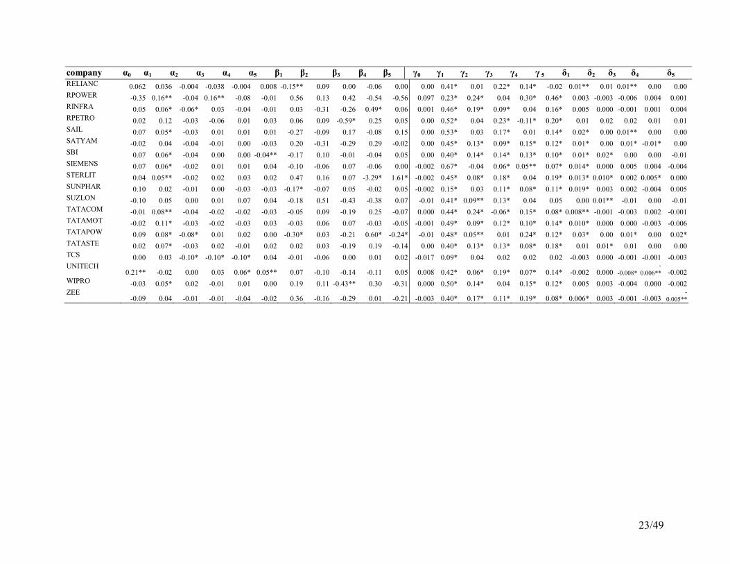
23/49
company α0 α1 α2 α3 α4 α5 β1 β2 β3 β4 β5 γ0 γ1 γ2 γ3 γ4 γ 5 δ1 δ2 δ3 δ4 δ5
RELIANC 0.062 0.036 -0.004 -0.038 -0.004 0.008 -0.15** 0.09 0.00 -0.06 0.00 0.00 0.41* 0.01 0.22* 0.14* -0.02 0.01** 0.01 0.01** 0.00 0.00
RPOWER -0.35 0.16** -0.04 0.16** -0.08 -0.01 0.56 0.13 0.42 -0.54 -0.56 0.097 0.23* 0.24* 0.04 0.30* 0.46* 0.003 -0.003 -0.006 0.004 0.001
RINFRA 0.05 0.06* -0.06* 0.03 -0.04 -0.01 0.03 -0.31 -0.26 0.49* 0.06 0.001 0.46* 0.19* 0.09* 0.04 0.16* 0.005 0.000 -0.001 0.001 0.004
RPETRO 0.02 0.12 -0.03 -0.06 0.01 0.03 0.06 0.09 -0.59* 0.25 0.05 0.00 0.52* 0.04 0.23* -0.11* 0.20* 0.01 0.02 0.02 0.01 0.01
SAIL 0.07 0.05* -0.03 0.01 0.01 0.01 -0.27 -0.09 0.17 -0.08 0.15 0.00 0.53* 0.03 0.17* 0.01 0.14* 0.02* 0.00 0.01** 0.00 0.00
SATYAM -0.02 0.04 -0.04 -0.01 0.00 -0.03 0.20 -0.31 -0.29 0.29 -0.02 0.00 0.45* 0.13* 0.09* 0.15* 0.12* 0.01* 0.00 0.01* -0.01* 0.00
SBI 0.07 0.06* -0.04 0.00 0.00 -0.04** -0.17 0.10 -0.01 -0.04 0.05 0.00 0.40* 0.14* 0.14* 0.13* 0.10* 0.01* 0.02* 0.00 0.00 -0.01
SIEMENS 0.07 0.06* -0.02 0.01 0.01 0.04 -0.10 -0.06 0.07 -0.06 0.00 -0.002 0.67* -0.04 0.06* 0.05** 0.07* 0.014* 0.000 0.005 0.004 -0.004
STERLIT 0.04 0.05** -0.02 0.02 0.03 0.02 0.47 0.16 0.07 -3.29* 1.61* -0.002 0.45* 0.08* 0.18* 0.04 0.19* 0.013* 0.010* 0.002 0.005* 0.000
SUNPHAR 0.10 0.02 -0.01 0.00 -0.03 -0.03 -0.17* -0.07 0.05 -0.02 0.05 -0.002 0.15* 0.03 0.11* 0.08* 0.11* 0.019* 0.003 0.002 -0.004 0.005
SUZLON -0.10 0.05 0.00 0.01 0.07 0.04 -0.18 0.51 -0.43 -0.38 0.07 -0.01 0.41* 0.09** 0.13* 0.04 0.05 0.00 0.01** -0.01 0.00 -0.01
TATACOM -0.01 0.08** -0.04 -0.02 -0.02 -0.03 -0.05 0.09 -0.19 0.25 -0.07 0.000 0.44* 0.24* -0.06* 0.15* 0.08* 0.008** -0.001 -0.003 0.002 -0.001
TATAMOT -0.02 0.11* -0.03 -0.02 -0.03 0.03 -0.03 0.06 0.07 -0.03 -0.05 -0.001 0.49* 0.09* 0.12* 0.10* 0.14* 0.010* 0.000 0.000 -0.003 -0.006 TATAPOW 0.09 0.08* -0.08* 0.01 0.02 0.00 -0.30* 0.03 -0.21 0.60* -0.24* -0.01 0.48* 0.05** 0.01 0.24* 0.12* 0.03* 0.00 0.01* 0.00 0.02*
TATASTE 0.02 0.07* -0.03 0.02 -0.01 0.02 0.02 0.03 -0.19 0.19 -0.14 0.00 0.40* 0.13* 0.13* 0.08* 0.18* 0.01 0.01* 0.01 0.00 0.00
TCS 0.00 0.03 -0.10* -0.10* -0.10* 0.04 -0.01 -0.06 0.00 0.01 0.02 -0.017 0.09* 0.04 0.02 0.02 0.02 -0.003 0.000 -0.001 -0.001 -0.003
UNITECH 0.21** -0.02 0.00 0.03 0.06* 0.05** 0.07 -0.10 -0.14 -0.11 0.05 0.008 0.42* 0.06* 0.19* 0.07* 0.14* -0.002 0.000 -0.008*
-
0.006** -0.002
WIPRO -0.03 0.05* 0.02 -0.01 0.01 0.00 0.19 0.11 -0.43** 0.30 -0.31 0.000 0.50* 0.14* 0.04 0.15* 0.12* 0.005 0.003 -0.004 0.000 -0.002
ZEE -0.09 0.04 -0.01 -0.01 -0.04 -0.02 0.36 -0.16 -0.29 0.01 -0.21 -0.003 0.40* 0.17* 0.11* 0.19* 0.08* 0.006* 0.003 -0.001 -0.003
-
0.005**
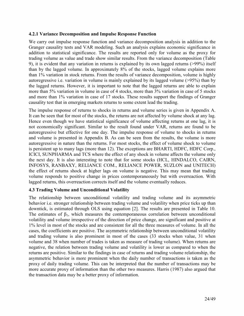
24/49
4.2.1 Variance Decomposition and Impulse Response Function
We carry out impulse response function and variance decomposition analysis in addition to the
Granger causality tests and VAR modeling. Such an analysis explains economic significance in
addition to statistical significance. The results are reported only for volume as the proxy for
trading volume as value and trade show similar results. From the variance decomposition (Table
9), it is evident that any variation in returns is explained by its own lagged returns (>99%) itself
than by the lagged volume. In approximately 8% of the stocks, lagged volume explains more
than 1% variation in stock returns. From the results of variance decomposition, volume is highly
autoregressive i.e. variation in volume is mainly explained by its lagged volume (>95%) than by
the lagged returns. However, it is important to note that the lagged returns are able to explain
more than 5% variation in volume in case of 4 stocks, more than 3% variation in case of 5 stocks
and more than 1% variation in case of 17 stocks. These results support the findings of Granger
causality test that in emerging markets returns to some extent lead the trading.
The impulse response of returns to shocks in returns and volume series is given in Appendix A.
It can be seen that for most of the stocks, the returns are not affected by volume shock at any lag.
Hence even though we have statistical significance of volume affecting returns at one lag, it is
not economically significant. Similar to the result found under VAR, returns are found to be
autoregressive but effective for one day. The impulse response of volume to shocks in returns
and volume is presented in Appendix B. As can be seen from the results, the volume is more
autoregressive in nature than the returns. For most stocks, the effect of volume shock to volume
is persistent up to many lags (more than 12). The exceptions are BHARTI, HDFC, HDFC Corp.,
ICICI, SUNPHARMA and TCS where the effect of any shock in volume affects the volume only
the next day. It is also interesting to note that for some stocks (HCL, HINDALCO, CAIRN,
INFOSYS, RANBAXY, RELIANCE COM., RELIANCE POWER, SUZLON and UNITECH)
the effect of returns shock at higher lags on volume is negative. This may mean that trading
volume responds to positive change in prices contemporaneously but with overreaction. With
lagged returns, this overreaction corrects itself and the volume eventually reduces.
4.3 Trading Volume and Unconditional Volatility
The relationship between unconditional volatility and trading volume and its asymmetric
behavior i.e. stronger relationship between trading volume and volatility when price ticks up than
downtick, is estimated through OLS using equation [2]. The results are presented in Table 10.
The estimates of β1, which measures the contemporaneous correlation between unconditional
volatility and volume irrespective of the direction of price change, are significant and positive at
1% level in most of the stocks and are consistent for all the three measures of volume. In all the
cases, the coefficients are positive. The asymmetric relationship between unconditional volatility
and trading volume is also prominent in most of the cases (33 stocks when value, 31 when
volume and 38 when number of trades is taken as measure of trading volume). When returns are
negative, the relation between trading volume and volatility is lower as compared to when the
returns are positive. Similar to the findings in case of returns and trading volume relationship, the
asymmetric behavior is more prominent when the daily number of transactions is taken as the
proxy of daily trading volume. This can be interpreted that the number of transactions may be
more accurate proxy of information than the other two measures. Harris (1987) also argued that
the transaction data may be a better proxy of information.

25/49
4.4. Trading Volume and Conditional Volatility
In order to investigate the effect of trading volume and conditional volatility, we first model the
time series of all the stock returns using GARCH (1,1) model. The parameter estimates of
GARCH (1,1) are presented in Table 11. It is found that for all stocks the conditional volatility is
time varying and shows persistence. The persistence of the conditional variance process, which
we measure by 1α +β1, is high (>0.9) except for DLF and is often close to unity.
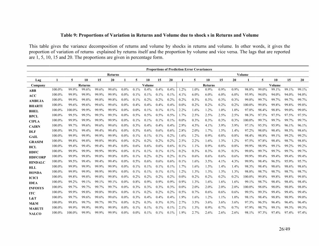
26/49
Table 9: Proportions of Variation in Returns and Volume due to shock s in Returns and Volume
This table gives the variance decomposition of returns and volume by shocks in returns and volume. In other words, it gives the
proportion of variation of returns explained by returns itself and the proportion by volume and vice versa. The lags that are reported
are 1, 5, 10, 15 and 20. The proportions are given in percentage form.
Proportions of Prediction Error Covariances
Returns Volume
Lag 1 5 10 15 20 1 5 10 15 20 1 5 10 15 20 1 5 10 15 20
Company Returns Volume Returns Volume
ABB 100.0% 99.9% 99.6% 99.6% 99.6% 0.0% 0.1% 0.4% 0.4% 0.4% 1.2% 1.0% 0.9% 0.9% 0.9% 98.8% 99.0% 99.1% 99.1% 99.1%
ACC 100.0% 99.9% 99.9% 99.9% 99.9% 0.0% 0.1% 0.1% 0.1% 0.1% 4.1% 6.0% 6.0% 6.0% 6.0% 95.9% 94.0% 94.0% 94.0% 94.0%
AMBUJA 100.0% 99.9% 99.8% 99.8% 99.8% 0.0% 0.1% 0.2% 0.2% 0.2% 0.2% 0.3% 0.3% 0.3% 0.3% 99.8% 99.7% 99.7% 99.7% 99.7%
BHARTI 100.0% 99.6% 99.6% 99.6% 99.6% 0.0% 0.4% 0.4% 0.4% 0.4% 0.0% 0.2% 0.2% 0.2% 0.2% 100.0% 99.8% 99.8% 99.8% 99.8%
BHEL 100.0% 100.0% 99.9% 99.9% 99.9% 0.0% 0.0% 0.1% 0.1% 0.1% 2.2% 1.6% 1.2% 1.0% 1.0% 97.8% 98.4% 98.8% 99.0% 99.0%
BPCL 100.0% 99.5% 99.5% 99.5% 99.5% 0.0% 0.5% 0.5% 0.5% 0.5% 1.7% 2.5% 2.5% 2.5% 2.5% 98.3% 97.5% 97.5% 97.5% 97.5%
CIPLA 100.0% 99.9% 99.9% 99.9% 99.9% 0.0% 0.1% 0.1% 0.1% 0.1% 0.0% 0.3% 0.3% 0.3% 0.3% 100.0% 99.7% 99.7% 99.7% 99.7%
CAIRN 100.0% 99.7% 99.6% 99.6% 99.6% 0.0% 0.3% 0.4% 0.4% 0.4% 2.9% 4.5% 4.1% 3.9% 3.9% 97.1% 95.5% 95.9% 96.1% 96.1%
DLF 100.0% 99.5% 99.4% 99.4% 99.4% 0.0% 0.5% 0.6% 0.6% 0.6% 2.8% 2.0% 1.7% 1.5% 1.4% 97.2% 98.0% 98.4% 98.5% 98.6%
GAIL 100.0% 99.9% 99.9% 99.9% 99.9% 0.0% 0.1% 0.1% 0.1% 0.2% 1.6% 1.2% 0.9% 0.8% 0.8% 98.4% 98.8% 99.1% 99.2% 99.2%
GRASIM 100.0% 99.8% 99.8% 99.8% 99.8% 0.0% 0.2% 0.2% 0.2% 0.2% 2.5% 2.2% 1.6% 1.3% 1.2% 97.5% 97.8% 98.4% 98.7% 98.8%
HCL 100.0% 99.4% 99.4% 99.4% 99.4% 0.0% 0.6% 0.6% 0.6% 0.6% 0.1% 1.1% 0.9% 0.8% 0.8% 99.9% 98.9% 99.1% 99.2% 99.2%
HDFC 100.0% 99.9% 99.9% 99.9% 99.9% 0.0% 0.1% 0.1% 0.1% 0.1% 0.2% 0.3% 0.3% 0.3% 0.3% 99.8% 99.7% 99.7% 99.7% 99.7%
HDFCORP 100.0% 99.9% 99.8% 99.8% 99.8% 0.0% 0.1% 0.2% 0.2% 0.2% 0.1% 0.6% 0.6% 0.6% 0.6% 99.9% 99.4% 99.4% 99.4% 99.4%
HINDALC 100.0% 99.5% 99.4% 99.4% 99.4% 0.0% 0.5% 0.6% 0.6% 0.6% 0.1% 1.6% 3.5% 4.1% 4.3% 99.9% 98.4% 96.5% 95.9% 95.7%
HLL 100.0% 99.9% 99.9% 99.9% 99.9% 0.0% 0.1% 0.1% 0.1% 0.1% 1.7% 1.6% 1.5% 1.4% 1.4% 98.3% 98.4% 98.6% 98.6% 98.6%
HONDA 100.0% 99.9% 99.9% 99.9% 99.9% 0.0% 0.1% 0.1% 0.1% 0.1% 1.2% 1.3% 1.3% 1.3% 1.3% 98.8% 98.7% 98.7% 98.7% 98.7%
ICICI 100.0% 99.8% 99.8% 99.8% 99.8% 0.0% 0.2% 0.2% 0.2% 0.2% 0.0% 0.2% 0.2% 0.2% 0.2% 100.0% 99.8% 99.8% 99.8% 99.8%
IDEA 100.0% 99.2% 99.1% 99.1% 99.1% 0.0% 0.8% 0.9% 0.9% 0.9% 0.9% 1.3% 1.6% 1.6% 1.6% 99.1% 98.7% 98.4% 98.4% 98.4%
INFOSYS 100.0% 99.7% 99.7% 99.7% 99.7% 0.0% 0.3% 0.3% 0.3% 0.3% 0.0% 2.0% 2.0% 2.0% 2.0% 100.0% 98.0% 98.0% 98.0% 98.0%
ITC 100.0% 99.9% 99.8% 99.8% 99.8% 0.0% 0.1% 0.2% 0.2% 0.2% 0.5% 0.7% 0.6% 0.6% 0.6% 99.5% 99.3% 99.4% 99.4% 99.4%
L&T 100.0% 99.7% 99.6% 99.6% 99.6% 0.0% 0.3% 0.4% 0.4% 0.4% 1.9% 1.6% 1.2% 1.1% 1.0% 98.1% 98.4% 98.8% 98.9% 99.0%
M&M 100.0% 99.8% 99.7% 99.7% 99.7% 0.0% 0.2% 0.3% 0.3% 0.3% 2.7% 3.5% 3.6% 3.6% 3.6% 97.3% 96.5% 96.4% 96.4% 96.4%
MARUTI 100.0% 99.9% 99.9% 99.9% 99.9% 0.0% 0.1% 0.1% 0.1% 0.1% 2.1% 1.3% 0.9% 0.7% 0.7% 97.9% 98.7% 99.1% 99.3% 99.3%
NALCO 100.0% 100.0% 99.9% 99.9% 99.9% 0.0% 0.0% 0.1% 0.1% 0.1% 1.9% 2.7% 2.6% 2.6% 2.6% 98.1% 97.3% 97.4% 97.4% 97.4%

27/49
NTPC 100.0% 99.6% 99.6% 99.6% 99.5% 0.0% 0.4% 0.4% 0.4% 0.5% 0.3% 1.2% 1.2% 1.2% 1.2% 99.7% 98.8% 98.8% 98.8% 98.8%
ONGC 100.0% 99.8% 99.7% 99.7% 99.7% 0.0% 0.2% 0.3% 0.3% 0.3% 0.2% 0.4% 0.3% 0.3% 0.3% 99.8% 99.6% 99.7% 99.7% 99.7%
PNB 100.0% 99.2% 99.1% 99.1% 99.1% 0.0% 0.8% 0.9% 0.9% 0.9% 8.4% 10.2% 10.7% 10.8% 10.8% 91.6% 89.8% 89.3% 89.2% 89.2%
POWER&G 100.0% 99.0% 98.8% 98.7% 98.7% 0.0% 1.0% 1.2% 1.3% 1.3% 0.3% 1.3% 2.5% 2.7% 2.9% 99.7% 98.7% 97.5% 97.3% 97.1%
RANBAXY 100.0% 99.7% 99.7% 99.6% 99.6% 0.0% 0.3% 0.4% 0.4% 0.4% 0.4% 0.6% 0.7% 0.7% 0.7% 99.6% 99.4% 99.3% 99.3% 99.3%
RCOMM 100.0% 99.4% 99.3% 99.3% 99.3% 0.0% 0.6% 0.7% 0.7% 0.7% 0.1% 1.1% 1.3% 1.3% 1.3% 99.9% 98.9% 98.7% 98.7% 98.7%
RELIANC 100.0% 99.8% 99.8% 99.8% 99.8% 0.0% 0.2% 0.2% 0.2% 0.2% 0.0% 0.4% 0.4% 0.4% 0.4% 100.0% 99.6% 99.6% 99.6% 99.7%
RPOWER 100.0% 98.6% 96.9% 96.1% 95.6% 0.0% 1.4% 3.1% 3.9% 4.4% 0.3% 0.3% 0.2% 0.1% 0.1% 99.7% 99.7% 99.8% 99.9% 99.9%
RINFRA 100.0% 99.7% 99.7% 99.7% 99.7% 0.0% 0.3% 0.3% 0.3% 0.3% 1.2% 1.0% 0.9% 0.8% 0.7% 98.8% 99.0% 99.1% 99.2% 99.3%
RPETRO 100.0% 99.3% 99.2% 99.2% 99.2% 0.0% 0.7% 0.8% 0.8% 0.8% 0.2% 3.4% 5.5% 6.3% 6.7% 99.8% 96.6% 94.5% 93.7% 93.3%
SAIL 100.0% 99.8% 99.7% 99.7% 99.7% 0.0% 0.2% 0.3% 0.3% 0.3% 5.6% 13.0% 14.5% 15.2% 15.6% 94.4% 87.0% 85.5% 84.8% 84.4%
SATYAM 100.0% 99.6% 99.6% 99.6% 99.6% 0.0% 0.4% 0.4% 0.4% 0.4% 0.0% 0.7% 1.9% 2.3% 2.4% 100.0% 99.3% 98.1% 97.7% 97.6%
SBI 100.0% 99.9% 99.9% 99.9% 99.9% 0.0% 0.1% 0.1% 0.1% 0.1% 1.5% 3.1% 3.0% 2.9% 2.9% 98.5% 96.9% 97.0% 97.1% 97.1%
SIEMENS 100.0% 99.7% 99.5% 99.4% 99.4% 0.0% 0.3% 0.5% 0.6% 0.6% 0.1% 0.5% 0.4% 0.4% 0.4% 99.9% 99.5% 99.6% 99.6% 99.6%
STERLIT 100.0% 97.7% 97.5% 97.3% 97.2% 0.0% 2.3% 2.5% 2.7% 2.8% 0.4% 1.3% 1.4% 1.4% 1.4% 99.6% 98.7% 98.6% 98.6% 98.6%
SUNPHAR 100.0% 99.7% 99.7% 99.7% 99.7% 0.0% 0.3% 0.3% 0.3% 0.3% 0.5% 0.8% 0.8% 0.8% 0.8% 99.5% 99.2% 99.2% 99.2% 99.2%
SUZLON 100.0% 96.7% 96.7% 96.6% 96.6% 0.0% 3.3% 3.3% 3.4% 3.4% 0.0% 0.3% 1.9% 2.4% 2.8% 100.0% 99.7% 98.1% 97.6% 97.2%
TATACOM 100.0% 99.8% 99.8% 99.8% 99.8% 0.0% 0.2% 0.2% 0.2% 0.2% 2.5% 3.1% 3.0% 3.0% 3.0% 97.5% 96.9% 97.0% 97.0% 97.0%
TATAMOT 100.0% 99.9% 99.8% 99.8% 99.8% 0.0% 0.1% 0.2% 0.2% 0.2% 2.3% 3.2% 2.6% 2.3% 2.2% 97.7% 96.8% 97.4% 97.7% 97.8%
TATAPOW 100.0% 99.4% 99.2% 99.2% 99.2% 0.0% 0.6% 0.8% 0.8% 0.8% 1.7% 4.1% 4.4% 4.5% 4.5% 98.3% 95.9% 95.6% 95.5% 95.5%
TATASTE 100.0% 99.7% 99.7% 99.7% 99.7% 0.0% 0.3% 0.3% 0.3% 0.3% 1.3% 1.8% 1.8% 1.8% 1.8% 98.7% 98.2% 98.2% 98.2% 98.2%
TCS 100.0% 99.9% 99.9% 99.9% 99.9% 0.0% 0.1% 0.1% 0.1% 0.1% 0.0% 0.2% 0.3% 0.3% 0.3% 100.0% 99.8% 99.7% 99.7% 99.7%
UNITECH 100.0% 99.6% 99.5% 99.5% 99.5% 0.0% 0.5% 0.5% 0.5% 0.5% 0.0% 3.7% 6.5% 7.8% 8.6% 100.0% 96.3% 93.5% 92.2% 91.4%
WIPRO 100.0% 99.9% 99.9% 99.9% 99.9% 0.0% 0.1% 0.1% 0.1% 0.1% 0.4% 0.5% 0.4% 0.4% 0.4% 99.6% 99.5% 99.6% 99.6% 99.6%
ZEE 100.0% 99.9% 99.9% 99.8% 99.8% 0.0% 0.1% 0.1% 0.2% 0.2% 3.7% 2.9% 2.2% 1.8% 1.7% 96.3% 97.1% 97.8% 98.2% 98.4%
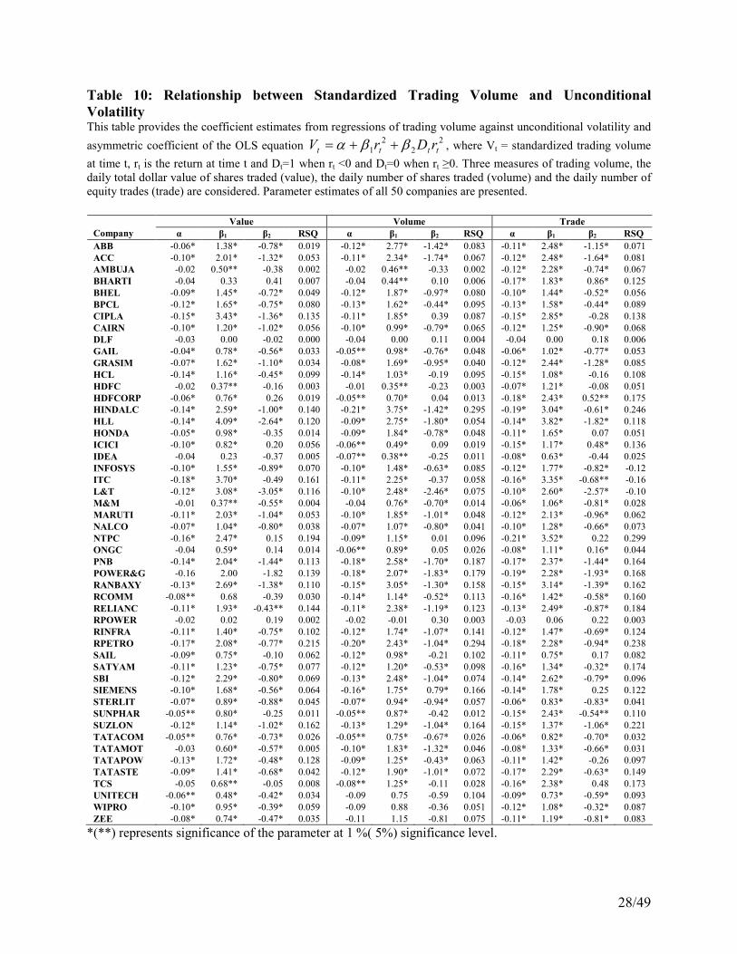
28/49
Table 10: Relationship between Standardized Trading Volume and Unconditional
Volatility This table provides the coefficient estimates from regressions of trading volume against unconditional volatility and
asymmetric coefficient of the OLS equation 2
2
2
1 tttt rDrV ββα ++= , where Vt = standardized trading volume
at time t, rt is the return at time t and Dt=1 when rt <0 and Dt=0 when rt ≥0. Three measures of trading volume, the
daily total dollar value of shares traded (value), the daily number of shares traded (volume) and the daily number of
equity trades (trade) are considered. Parameter estimates of all 50 companies are presented.
Value Volume Trade
Company α β1 β2 RSQ α β1 β2 RSQ α β1 β2 RSQ
ABB -0.06* 1.38* -0.78* 0.019 -0.12* 2.77* -1.42* 0.083 -0.11* 2.48* -1.15* 0.071
ACC -0.10* 2.01* -1.32* 0.053 -0.11* 2.34* -1.74* 0.067 -0.12* 2.48* -1.64* 0.081
AMBUJA -0.02 0.50** -0.38 0.002 -0.02 0.46** -0.33 0.002 -0.12* 2.28* -0.74* 0.067
BHARTI -0.04 0.33 0.41 0.007 -0.04 0.44** 0.10 0.006 -0.17* 1.83* 0.86* 0.125
BHEL -0.09* 1.45* -0.72* 0.049 -0.12* 1.87* -0.97* 0.080 -0.10* 1.44* -0.52* 0.056
BPCL -0.12* 1.65* -0.75* 0.080 -0.13* 1.62* -0.44* 0.095 -0.13* 1.58* -0.44* 0.089
CIPLA -0.15* 3.43* -1.36* 0.135 -0.11* 1.85* 0.39 0.087 -0.15* 2.85* -0.28 0.138
CAIRN -0.10* 1.20* -1.02* 0.056 -0.10* 0.99* -0.79* 0.065 -0.12* 1.25* -0.90* 0.068
DLF -0.03 0.00 -0.02 0.000 -0.04 0.00 0.11 0.004 -0.04 0.00 0.18 0.006
GAIL -0.04* 0.78* -0.56* 0.033 -0.05** 0.98* -0.76* 0.048 -0.06* 1.02* -0.77* 0.053
GRASIM -0.07* 1.62* -1.10* 0.034 -0.08* 1.69* -0.95* 0.040 -0.12* 2.44* -1.28* 0.085
HCL -0.14* 1.16* -0.45* 0.099 -0.14* 1.03* -0.19 0.095 -0.15* 1.08* -0.16 0.108
HDFC -0.02 0.37** -0.16 0.003 -0.01 0.35** -0.23 0.003 -0.07* 1.21* -0.08 0.051
HDFCORP -0.06* 0.76* 0.26 0.019 -0.05** 0.70* 0.04 0.013 -0.18* 2.43* 0.52** 0.175
HINDALC -0.14* 2.59* -1.00* 0.140 -0.21* 3.75* -1.42* 0.295 -0.19* 3.04* -0.61* 0.246
HLL -0.14* 4.09* -2.64* 0.120 -0.09* 2.75* -1.80* 0.054 -0.14* 3.82* -1.82* 0.118
HONDA -0.05* 0.98* -0.35 0.014 -0.09* 1.84* -0.78* 0.048 -0.11* 1.65* 0.07 0.051
ICICI -0.10* 0.82* 0.20 0.056 -0.06** 0.49* 0.09 0.019 -0.15* 1.17* 0.48* 0.136
IDEA -0.04 0.23 -0.37 0.005 -0.07** 0.38** -0.25 0.011 -0.08* 0.63* -0.44 0.025
INFOSYS -0.10* 1.55* -0.89* 0.070 -0.10* 1.48* -0.63* 0.085 -0.12* 1.77* -0.82* -0.12
ITC -0.18* 3.70* -0.49 0.161 -0.11* 2.25* -0.37 0.058 -0.16* 3.35* -0.68** -0.16
L&T -0.12* 3.08* -3.05* 0.116 -0.10* 2.48* -2.46* 0.075 -0.10* 2.60* -2.57* -0.10
M&M -0.01 0.37** -0.55* 0.004 -0.04 0.76* -0.70* 0.014 -0.06* 1.06* -0.81* 0.028
MARUTI -0.11* 2.03* -1.04* 0.053 -0.10* 1.85* -1.01* 0.048 -0.12* 2.13* -0.96* 0.062
NALCO -0.07* 1.04* -0.80* 0.038 -0.07* 1.07* -0.80* 0.041 -0.10* 1.28* -0.66* 0.073
NTPC -0.16* 2.47* 0.15 0.194 -0.09* 1.15* 0.01 0.096 -0.21* 3.52* 0.22 0.299
ONGC -0.04 0.59* 0.14 0.014 -0.06** 0.89* 0.05 0.026 -0.08* 1.11* 0.16* 0.044
PNB -0.14* 2.04* -1.44* 0.113 -0.18* 2.58* -1.70* 0.187 -0.17* 2.37* -1.44* 0.164
POWER&G -0.16 2.00 -1.82 0.139 -0.18* 2.07* -1.83* 0.179 -0.19* 2.28* -1.93* 0.168
RANBAXY -0.13* 2.69* -1.38* 0.110 -0.15* 3.05* -1.30* 0.158 -0.15* 3.14* -1.39* 0.162
RCOMM -0.08** 0.68 -0.39 0.030 -0.14* 1.14* -0.52* 0.113 -0.16* 1.42* -0.58* 0.160
RELIANC -0.11* 1.93* -0.43** 0.144 -0.11* 2.38* -1.19* 0.123 -0.13* 2.49* -0.87* 0.184
RPOWER -0.02 0.02 0.19 0.002 -0.02 -0.01 0.30 0.003 -0.03 0.06 0.22 0.003
RINFRA -0.11* 1.40* -0.75* 0.102 -0.12* 1.74* -1.07* 0.141 -0.12* 1.47* -0.69* 0.124
RPETRO -0.17* 2.08* -0.77* 0.215 -0.20* 2.43* -1.04* 0.294 -0.18* 2.28* -0.94* 0.238
SAIL -0.09* 0.75* -0.10 0.062 -0.12* 0.98* -0.21 0.102 -0.11* 0.75* 0.17 0.082
SATYAM -0.11* 1.23* -0.75* 0.077 -0.12* 1.20* -0.53* 0.098 -0.16* 1.34* -0.32* 0.174
SBI -0.12* 2.29* -0.80* 0.069 -0.13* 2.48* -1.04* 0.074 -0.14* 2.62* -0.79* 0.096
SIEMENS -0.10* 1.68* -0.56* 0.064 -0.16* 1.75* 0.79* 0.166 -0.14* 1.78* 0.25 0.122
STERLIT -0.07* 0.89* -0.88* 0.045 -0.07* 0.94* -0.94* 0.057 -0.06* 0.83* -0.83* 0.041
SUNPHAR -0.05** 0.80* -0.25 0.011 -0.05** 0.87* -0.42 0.012 -0.15* 2.43* -0.54** 0.110
SUZLON -0.12* 1.14* -1.02* 0.162 -0.13* 1.29* -1.04* 0.164 -0.15* 1.37* -1.06* 0.221
TATACOM -0.05** 0.76* -0.73* 0.026 -0.05** 0.75* -0.67* 0.026 -0.06* 0.82* -0.70* 0.032
TATAMOT -0.03 0.60* -0.57* 0.005 -0.10* 1.83* -1.32* 0.046 -0.08* 1.33* -0.66* 0.031
TATAPOW -0.13* 1.72* -0.48* 0.128 -0.09* 1.25* -0.43* 0.063 -0.11* 1.42* -0.26 0.097
TATASTE -0.09* 1.41* -0.68* 0.042 -0.12* 1.90* -1.01* 0.072 -0.17* 2.29* -0.63* 0.149
TCS -0.05 0.68** -0.05 0.008 -0.08** 1.25* -0.11 0.028 -0.16* 2.38* 0.48 0.173
UNITECH -0.06** 0.48* -0.42* 0.034 -0.09 0.75 -0.59 0.104 -0.09* 0.73* -0.59* 0.093
WIPRO -0.10* 0.95* -0.39* 0.059 -0.09 0.88 -0.36 0.051 -0.12* 1.08* -0.32* 0.087
ZEE -0.08* 0.74* -0.47* 0.035 -0.11 1.15 -0.81 0.075 -0.11* 1.19* -0.81* 0.083
*(**) represents significance of the parameter at 1 %( 5%) significance level.
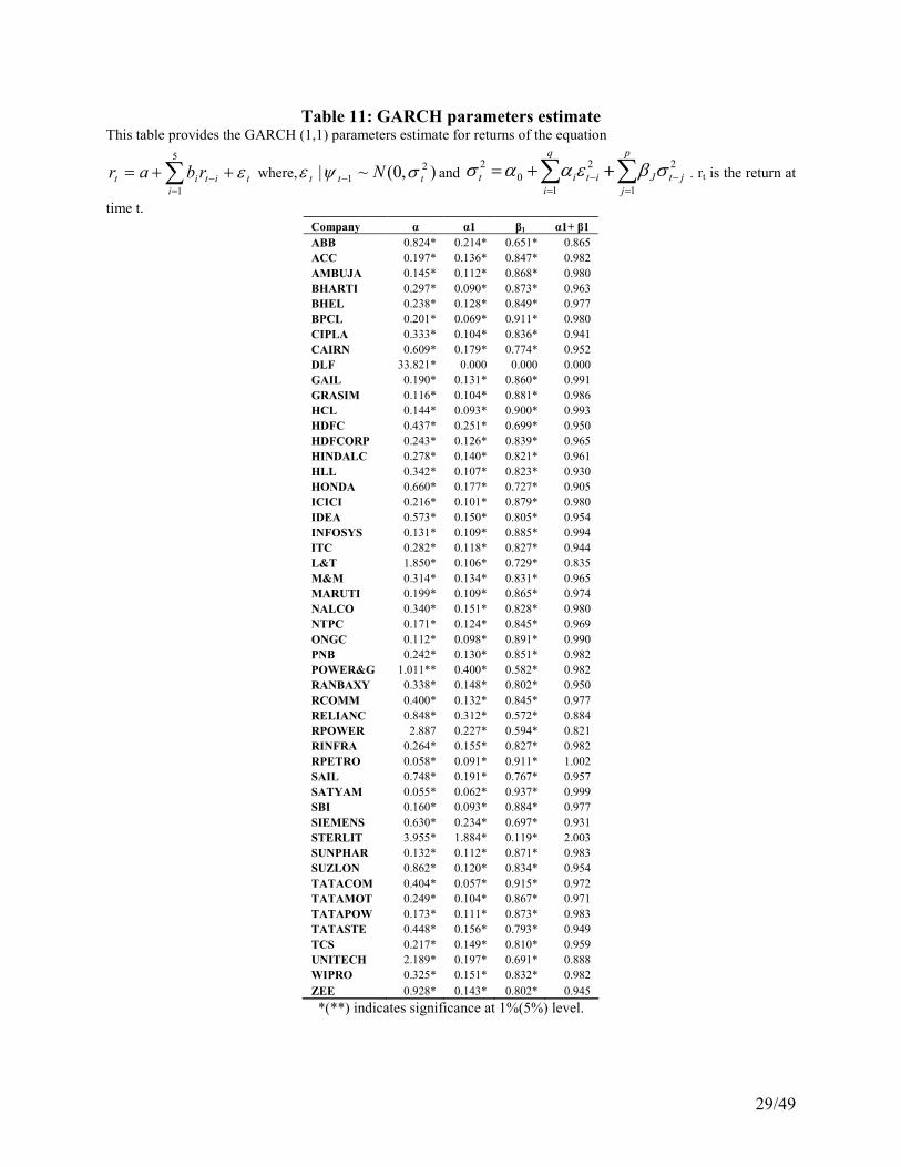
29/49
Table 11: GARCH parameters estimate This table provides the GARCH (1,1) parameters estimate for returns of the equation
t
i
itit rbar ε++= ∑=
−
5
1
where, ),0(~| 2
1 ttt N σψε − and ∑∑=
−=
− ++=p
j
jtJ
q
i
itit
1
2
1
2
0
2 σβεαασ . rt is the return at
time t.
Company α α1 β1 α1+ β1
ABB 0.824* 0.214* 0.651* 0.865
ACC 0.197* 0.136* 0.847* 0.982
AMBUJA 0.145* 0.112* 0.868* 0.980
BHARTI 0.297* 0.090* 0.873* 0.963
BHEL 0.238* 0.128* 0.849* 0.977
BPCL 0.201* 0.069* 0.911* 0.980
CIPLA 0.333* 0.104* 0.836* 0.941
CAIRN 0.609* 0.179* 0.774* 0.952
DLF 33.821* 0.000 0.000 0.000
GAIL 0.190* 0.131* 0.860* 0.991
GRASIM 0.116* 0.104* 0.881* 0.986
HCL 0.144* 0.093* 0.900* 0.993
HDFC 0.437* 0.251* 0.699* 0.950
HDFCORP 0.243* 0.126* 0.839* 0.965
HINDALC 0.278* 0.140* 0.821* 0.961
HLL 0.342* 0.107* 0.823* 0.930
HONDA 0.660* 0.177* 0.727* 0.905
ICICI 0.216* 0.101* 0.879* 0.980
IDEA 0.573* 0.150* 0.805* 0.954
INFOSYS 0.131* 0.109* 0.885* 0.994
ITC 0.282* 0.118* 0.827* 0.944
L&T 1.850* 0.106* 0.729* 0.835
M&M 0.314* 0.134* 0.831* 0.965
MARUTI 0.199* 0.109* 0.865* 0.974
NALCO 0.340* 0.151* 0.828* 0.980
NTPC 0.171* 0.124* 0.845* 0.969
ONGC 0.112* 0.098* 0.891* 0.990
PNB 0.242* 0.130* 0.851* 0.982
POWER&G 1.011** 0.400* 0.582* 0.982
RANBAXY 0.338* 0.148* 0.802* 0.950
RCOMM 0.400* 0.132* 0.845* 0.977
RELIANC 0.848* 0.312* 0.572* 0.884
RPOWER 2.887 0.227* 0.594* 0.821
RINFRA 0.264* 0.155* 0.827* 0.982
RPETRO 0.058* 0.091* 0.911* 1.002
SAIL 0.748* 0.191* 0.767* 0.957
SATYAM 0.055* 0.062* 0.937* 0.999
SBI 0.160* 0.093* 0.884* 0.977
SIEMENS 0.630* 0.234* 0.697* 0.931
STERLIT 3.955* 1.884* 0.119* 2.003
SUNPHAR 0.132* 0.112* 0.871* 0.983
SUZLON 0.862* 0.120* 0.834* 0.954
TATACOM 0.404* 0.057* 0.915* 0.972
TATAMOT 0.249* 0.104* 0.867* 0.971
TATAPOW 0.173* 0.111* 0.873* 0.983
TATASTE 0.448* 0.156* 0.793* 0.949
TCS 0.217* 0.149* 0.810* 0.959
UNITECH 2.189* 0.197* 0.691* 0.888
WIPRO 0.325* 0.151* 0.832* 0.982
ZEE 0.928* 0.143* 0.802* 0.945
*(**) indicates significance at 1%(5%) level.
30/49
In most of the cases, the autoregressive parameter of conditional volatility is higher than the
return innovations (except for STERLITE). The mixed distribution hypothesis or the relationship
between conditional volatility and trading volume is then estimated by modifying GARCH
equation as explained in equation [5].The MDH model predicts that if trading volume is a proxy
of information and if daily volume is serially correlated then the parameter χ> 0 and ( 1α +β1) will
become either small or statistically insignificant. The persistence of variance as measured by
( 1α +β1) should become negligible if accounting for the uneven flow of information (V) explains
the presence of ARCH effect in the data. The contemporaneous trading volume (V) is assumed
as the proxy of information5. The parameter estimates of equation [5] are presented in Table 12.
In most cases, the inclusion of trading volume as an explanatory variable in the conditional
variance equation results in a substantial reduction of volatility persistence in daily returns.
Hence, serially correlated news arrival processes proxied by trading volume as a source of
ARCH effect is indicated by results in the Indian stock market. It is found that around 80% of the
companies have trading volume as significant explanatory variable (across all three measures).
In approximately 34% of the stocks the GARCH parameters become statistically insignificant
and in case of another 44%, the persistence reduces dramatically when volume is used as an
explanatory variable in the conditional volatility equation. In 18 stocks, the explanatory power of
GARCH is not reduced by the inclusion of trading volume as explanatory variable. When value
is used, the GARCH effect becomes insignificant in 16% cases only and when trade is used, 54%
stocks show insignificant GARCH effect. However, in all stocks the volume parameter is
positive and significant at 1% significant level. This result supports strong relationship between
contemporaneous trading volume and conditional volatility. However, our results provide mixed
conclusions, not entirely rejecting the MDH nor giving it an unconditional support in case of
Indian stock market. Similar results have been reported by Ane and Ureche-Rangau (2008). Ane
and Ureche-Rangau (2008) analyzed the temporal dependence of volatility and volume on 50
LSE stocks and found mixed results. They found that in some stocks the effect of volume is very
strong, in some moderate and in some cases it has negligible effect. They tried to explain these
differences by understanding the long term behavior of volume and volatility and found that the
stocks for which the trading volume has negligible explanatory power as compared to the ARCH
effect, have highest difference in the fractional differencing parameter of volume and volatility.
It is possible that these two variables do share common short-term movements, but they may
have fundamentally different long-term behavior.
Other results which support MDH over ARCH effect for most of the stocks are in line with the
findings of Lamoureax and Lastrapes (1990), Kim & Kon, (1994), Gallo & Pacini, (2000), and
Omran & McKenzie (2000) in developed markets and Pyun, Lee, and Nam (2000) and Bohl and
Henke (2003) in emerging market. Pyun, Lee, and Nam (2000) studied 15 individual shares of
the Korean stock market and found that all stocks show high statistically significant positive
correlation with contemporaneous volume. They found that as the volume is used in GARCH
equation as an exogenous variable the return volatility persistence reduces dramatically. Bohl
and Henke (2003) investigated 20 Polish stocks and found that in majority of cases volatility
persistence tends to disappear when trading volume is included in the conditional variance
equation.
5 In most of the stocks and across all three measures of trading volume, we found very high autocorrelation. This
fact validates one of the assumption of MDH.

31/49
Table 11: GARCH parameters estimate with trading volatility as one of the exogenous
variable of the GARCH equation This table provides the GARCH (1,1) parameters estimate for returns of the equation
t
i
itit rbar ε++= ∑=
−
5
1
where, ),0(~| 2
1 ttt N σψε − and t
p
j
jtJ
q
i
itit Vχσβεαασ +++= ∑∑=
−=
−1
2
1
2
0
2. rt is the
return at time t and Vt is standardized trading volume at time t. Three measures of trading volume, the daily total
dollar value of shares traded (value), the daily number of shares traded (volume) and the daily number of equity
trades (trade) are considered.
*indicates significance at the 1% level.
Value Volume Trade Company
α β1 β1 χ α β1 β1 χ α β1 β1 Χ
ABB 1.131* 0.258* 0.560* 0.818 0.34* 5.015* 0.209* 0.000 0.209 5.80* 5.208* 0.229* 0.000 0.229 5.52*
ACC 0.573* 0.161* 0.771* 0.932 0.47* 3.569* 0.253* 0.310* 0.564 3.38* 6.235* 0.196* 0.001 0.197 5.04*
AMBUJA 0.174* 0.117* 0.858* 0.975 0.11 0.171* 0.116* 0.859* 0.975 0.10** 4.429* 0.297* 0.068** 0.365 4.05*
BHARTI 1.949* 0.215* 0.555* 0.770 2.67* 8.439* 0.153* 0.000 0.153 33.59* 6.581* 0.144* 0.000 0.144 4.92*
BHEL 5.237* 0.333* 0.151* 0.485 4.95* 8.495* 0.176* 0.000 0.176 11.84* 8.650* 0.216* 0.000 0.216 11.73*
BPCL 2.329* 0.255* 0.511* 0.766 1.36* 6.127* 0.282* 0.088** 0.370 4.41* 6.304* 0.293* 0.068 0.361 4.617*
CIPLA 4.364* 0.215* 0.054* 0.269 5.29* 4.389* 0.281* 0.047* 0.327 4.85* 4.254* 0.230* 0.032* 0.262 4.65*
CAIRN 4.744* 0.384* 0.305* 0.689 5.86* 5.877* 0.381* 0.222* 0.603 7.95* 10.46* 0.310* 0.000 0.310 13.35*
DLF 32.67* 0.000 0.002 0.002 0.00 33.84* 0.000 0.000 0.000 1.25 33.83* 0.000 0.000 0.000 0.00
GAIL 5.781* 0.351* 0.165* 0.516 6.17* 0.349* 0.145* 0.830* 0.975 0.30* 0.575* 0.162* 0.790* 0.953 0.55*
GRASIM 0.230* 0.120* 0.847* 0.967 0.16* 0.548* 0.170* 0.761* 0.932 0.66* 4.381* 0.271* 0.116* 0.387 4.09*
HCL 4.797* 0.415* 0.325* 0.740 5.41* 1.152* 0.189* 0.746* 0.935 1.64* 2.689* 0.263* 0.583* 0.846 3.29*
HDFC 1.248* 0.295* 0.550* 0.845 2.85* 5.877* 0.230* 0.013 0.242 18.85* 5.530* 0.191* 0.000 0.191 8.33*
HDFCORP 4.139* 0.230* 0.269* 0.499 9.41* 6.219* 0.139* 0.089* 0.228 15.85* 6.288* 0.108* 0.000 0.108 9.95*
HINDALC 3.928* 0.296* 0.150* 0.445 3.86* 0.807* 0.183* 0.700* 0.883 0.64* 5.123* 0.279* 0.040 0.319 5.61*
HLL 4.301* 0.149* 0.025 0.173 4.38* 1.983* 0.259* 0.348* 0.608 1.25* 3.867* 0.157* 0.005 0.162 3.05*
HONDA 0.790* 0.197* 0.689* 0.886 0.21* 1.032* 0.204* 0.645* 0.849 0.49* 4.888* 0.245* 0.000 0.245 2.94*
ICICI 0.283* 0.094* 0.879* 0.973 0.20* 0.335* 0.099* 0.869* 0.968 0.64* 0.323* 0.099* 0.870* 0.969 0.21*
IDEA 0.468* 0.216* 0.761* 0.978 0.34 0.684* 0.180* 0.771* 0.951 0.56 0.605* 0.170* 0.786* 0.955 0.20
INFOSYS 5.538* 0.301* 0.146* 0.447 6.20* 5.281* 0.184* 0.172* 0.356 4.47* 4.844* 0.203* 0.149* 0.353 3.50*
ITC 3.418* 0.231* 0.135* 0.366 3.60* 2.694* 0.297* 0.236* 0.533 2.38* 3.765* 0.249* 0.018 0.267 3.11*
L&T 12.75* 0.044* 0.000 0.044 14.71* 9.298* 0.067* 0.013 0.081 3.50* 11.06* 0.000 0.000 0.000 9.25*
M&M 0.340* 0.143* 0.819* 0.961 0.05 0.453* 0.148* 0.799* 0.947 0.19* 0.464* 0.154* 0.793* 0.947 0.12*
MARUTI 0.256* 0.117* 0.849* 0.966 0.08 0.239* 0.112* 0.856* 0.969 0.05 6.340* 0.119* 0.000 0.119 3.91*
NALCO 0.490* 0.222* 0.764* 0.985 0.20* 0.551* 0.206* 0.765* 0.972 0.37* 0.760* 0.216* 0.738* 0.954 0.41*
NTPC 5.180* 0.102* 0.000 0.102 6.76* 5.347* 0.090* 0.000 0.090 10.41* 5.267* 0.021 0.000 0.021 5.90*
ONGC 0.134* 0.108* 0.879* 0.988 0.06* 0.148* 0.111* 0.875* 0.986 0.07* 0.141* 0.107* 0.880* 0.987 0.03*
PNB 1.142* 0.224* 0.669* 0.893 0.86* 8.464* 0.206* 0.000 0.206 9.31* 7.709* 0.202* 0.000 0.202 6.35*
POWER&G 1.508* 0.488* 0.497* 0.985 1.57 2.412* 0.474* 0.466* 0.939 4.20** 10.65* 0.319* 0.000 0.319 14.61*
RANBAXY 5.352* 0.225* 0.011 0.236 7.33* 5.601* 0.141* 0.000 0.141 7.82* 5.129* 0.166* 0.000 0.166 6.52*
RCOMM 9.976* 0.243* 0.085* 0.328 8.42* 9.449* 0.074** 0.155** 0.229 8.33* 9.652* 0.394* 0.001 0.395 7.55*
RELIANC 3.673* 0.334* 0.063* 0.397 3.03* 2.385* 0.381* 0.267* 0.648 1.97* 4.427* 0.262* 0.000 0.262 4.14*
RPOWER 2.698 0.225* 0.609* 0.834 0.95 3.087 0.230* 0.580* 0.810 0.86 2.984 0.221* 0.597* 0.817 1.12
RINFRA 4.509* 0.306* 0.337* 0.642 7.42* 8.659* 0.206* 0.000 0.206 12.70* 11.10* 0.251* 0.000 0.251 19.43*
RPETRO 6.956* 0.269* 0.090 0.359 9.87* 8.566* 0.065 0.007 0.072 10.27* 10.09* 0.077 0.000 0.077 11.24*
SAIL 1.106* 0.215* 0.717* 0.933 0.46* 10.783* 0.290* 0.000 0.290 11.65* 1.832* 0.239* 0.640* 0.879 0.83*
SATYAM 5.890* 0.313* 0.301* 0.614 5.66* 1.930* 0.226* 0.648* 0.875 1.59* 6.960* 0.286* 0.186* 0.472 5.73*
SBI 4.804* 0.223* 0.024 0.247 2.47* 0.336* 0.113* 0.837* 0.950 0.15* 5.186* 0.210* 0.000 0.210 3.53*
SIEMENS 1.904* 0.314* 0.450* 0.764 1.72* 5.764* 0.231* 0.017 0.248 7.14* 5.321* 0.291* 0.038 0.328 5.92*
STERLIT 14.15* 0.673* 0.003 0.676 10.97* 22.911* 0.256* 0.000 0.256 32.01* 14.81* 0.143* 0.418* 0.562 20.40*
SUNPHAR 0.744* 0.257* 0.646* 0.903 0.83* 1.188* 0.298* 0.545 0.843 1.70* 3.996* 0.329* 0.082* 0.411 3.78*
SUZLON 14.69* 0.17* 0.009 0.184 16.3* 25.286* 0.084** 0.000 0.084 51.98* 18.54* 0.058 0.002 0.059 24.74*
TATACOM 9.35* 0.35* 0.09* 0.448 11.0* 6.530* 0.426* 0.203* 0.629 6.60* 7.564* 0.432* 0.169* 0.602 8.57*
TATAMOT 0.26* 0.10* 0.86* 0.969 0.00 0.286* 0.107* 0.859* 0.966 0.04 0.249* 0.104* 0.867* 0.971 0.00
TATAPOW 1.29* 0.21* 0.64* 0.856 0.7* 0.308* 0.114* 0.853* 0.967 0.20* 5.378* 0.274* 0.104* 0.378 4.20*
TATASTE 0.95* 0.207* 0.682* 0.889 0.36* 1.543* 0.245* 0.576* 0.821 0.73* 1.522* 0.234* 0.589* 0.823 0.67*
TCS 0.211* 0.154* 0.808* 0.961 0.01 3.699* 0.274* 0.107* 0.382 6.27* 3.950* 0.126* 0.052 0.178 3.74*
UNITECH 11.1* 0.292* 0.144** 0.436 5.19* 6.035* 0.228* 0.470* 0.698 6.29* 4.071* 0.233* 0.556* 0.790 1.57*
WIPRO 5.632* 0.366* 0.311* 0.677 7.08* 3.615* 0.397* 0.366* 0.763 3.72* 4.652* 0.375* 0.312* 0.687 4.60*
ZEE 7.99* 0.30* 0.247* 0.547 8.42* 11.543* 0.281* 0.031 0.313 10.79* 12.02* 0.259* 0.000 0.259 9.96*
32/49
In line with such empirical evidence in other emerging markets, our result partially supports the
implications of the MDH which provides, to a large extent, a valid theoretical explanation for
behavior of volatility. However, our results are mixed as opposed to the findings of Sharma et al.
(1996), Chen (2001) Argo and Nieto (2005) who found that the total trading volume is unable to
eliminate the ARCH effect.
5. Conclusions
Understanding the relationship between returns, volatility and trading volume in financial
markets is equally important for traders, researchers and policy makers. The distribution of
returns has implications for various financial models and risk management practices. The
dynamic relationship between returns and trading volume helps to understand the market
clearing process and frictions in the market. Also, implications of trading volume in forecasting
volatility helps agents like traders, with a very short-term investment horizon and many portfolio
managers that have a medium- to long-term investment horizon. In emerging markets generally
and in Indian stock market context specifically, very few empirical studies has been reported on
aforementioned issues. This paper reports an empirical study for Indian Stock market.
Using 50 Indian stocks, we analyze the returns and volume relationship, focusing on the
contemporaneous relation between absolute returns and trading volume, the asymmetric behavior
of trading volume in response to price changes and dynamic (lead-lag) relationship between
returns and trading volume. We model the dynamic relationship using VAR model. This study
also investigates the contemporaneous relationship between volatility and trading volume. In this
study we generalize the work of Lamoureax and Lastrapes (1990) which supports the influence
of trading volume on the persistence of GARCH effects on the returns of the financial assets.
Our findings indicate evidence of positive contemporaneous correlation between absolute price
changes and trading volume in Indian stock markets. However, we get mixed result on
asymmetric relationship between trading volume and returns. Most of the stocks show
asymmetric behavior which is in line with the findings of Assogbavi et al. (1995) and Brailsford
(1996). Some of the stocks, where we do not find asymmetric behavior, are consistent with the
findings of Assogbavi (2007) that clearly indicated the absence of asymmetric relationship in
emerging markets. The results of dynamic relationship between returns and trading volume show
very interesting results. We find strong evidence that in Indian market, past returns Granger
cause trading volume, which can easily conceived in an emerging market (Assogbavi, 2007)
where the state of development of the market possibly does not allow instantaneous information
dissemination. Our results are further supported by the variance decomposition. However, in
most of the cases the relationship lacks economic significance even when statistically significant.
The results of impulse response analysis indicate that both returns and volume are mostly
affected by their own lag and the volume is more autoregressive than returns i.e. any shock in
either returns or volume does not affect the return series beyond one lag.
In case of unconditional volatility and trading volume, we find positive contemporaneous
relationship between trading volume and unconditional volatility. However, the results on
asymmetric relationship are mixed. In most of the cases, there exists asymmetric relationship and
relationship is stronger when prices move up than when prices go down. In some stocks, we do
33/49
not find such asymmetric relationship. The results of relation between trading volume and
conditional volatility support strong contemporaneous relationship between trading volume and
conditional volatility. However, our results are mixed. They do not entirely reject the MDH nor
give it an unconditional support. In more than 70% of the stocks, ARCH effect is either reduced
or becomes insignificant when trading volume is included in GARCH equation. It indicates that
the trading volume is a better proxy of information than the volatility itself. However for some
stocks the GARCH parameters do not reduce. Similar kind of mixed results have been found for
LSE stocks by Ane and Ureche-Rangau (2008). Our results also indicate that in Indian stock
markets, the daily number of transactions may be a better proxy of information than the total
number of shares traded or the total value of shares traded.
34/49
References
Abdullah, D.A. and P.C. Rangazas (1988). "Money and the Business Cycle: Another Look",
Review of Economics and Statistics, 70, 680-85.
Admati, A.R. and Pfleiderer, P., (1988). "A Theory of Intraday Trading Patterns: Volume and
Price Variability", Review of Financial Studies, 1,3-40.
Andersen, T. (1996). “Return volatility and trading volume: An information flow interpretation
of stochastic volatility”, Journal of Finance, 51, 169–204.
Ane, T. Amd Ureche-Rangau, L. (2008).“ Does trading volume really explain stock returns
volatility?”, Journal of International Financial Markets, Institutions, and Money, 18, 216–
235.
Argo, V. and Nieto, L. (2005). “Heteroskedasticity in the returns of the main world stock
exchange indices: volume versus GARCH effects”, Journal of International Financial
Markets, Institutions, and Money, 15, 271–384.
Assogbavi, T. (2007) “Equity Price-Volume Relationship On The Russian Stock Exchange”,
International Business & Economics Research Journal, Vol 6, 9, 107-116.
Assogbavi, T., Khoury, N., and Yourougou, P. (1995). “Short interest and the asymmetry of the
price-volume relationship in the Canadian Stock market”, Journal of Banking & Finance
19 1341-1358
Bhagat, S., Bhatia. S. (1996). “Trading Volume and Price Variability: Evidence on Lead-Lag
Relations for Granger-Causality Tests”, Working paper, University of Colorado at
Boulder.
Bohl, M. T., and Henke, H. (2003). “Trading volume and stock market volatility: The Polish
case”, International Review of Financial Analysis, 12, 513–525
Blume, L., Easley, D., and O’Hara, M. (1994). “Market statistics and technical analysis: The role
of volume”, Journal of Finance, 491, 153-182.
Brailsford, T. (1996). “The empirical relationship between trading volume, returns, and
volatility”, Accounting and Finance, 35, 89–111.
Chen, K. and Fong W. N., (2000). “Trade size, order imbalance, and the volatility-volume
relation”, Journal of Financial Economics, 57, 247-273.
Chen, G. M., Firth, M., and Rui, O. M. (2001). “Dynamic relation between stock returns, trading
volume, and volatility”. Financial Review, 36, 153–73.
35/49
Chordia, T. and Swaminathan, B. (2000). “Trading volume and cross-autocorrelations in stock
returns”, Journal of Finance, 55,913-935.
Clark, P.K. (1973). “A subordinated stochastic process model with finite variance for speculative
prices”, Econometrica, 41, 135-55.
Copeland, T. E. (1976). “A model of asset trading under the assumption of sequential
information arrival”, Journal of Finance 31, 1149-1168.
Crouch, R. L., (1970). “The volume of transactions and price changes on the New York Stock
Exchange”, Financial Analysts Journal, 26, 104-109.
Epps, T., Epps, M. (1976). “The stochastic dependence of security price changes and transaction
volumes: Implications for the mixture-of-distributions hypothesis”, Econometrica, 44,
305}321.
Foster, F.D. and Viswanathan, S. (1990). "A Theory of Interday Variations in Volume, Variance
and Trading Costs in Securities Markets", Review of Financial Studies, 3, 593-624.
Gallo, G., & Pacini, B. (2000). “The effects of trading activity on market volatility”, European
Journal of Finance, 6, 163–175.
Grundy, B., and McNichols, M. (1989). “Trade and revelation of information through prices and
direct disclosure”, “Review of Financial Studies, 2, 495-526.
Harris, L. (1986). “Cross-security tests of the mixture of distributions hypothesis”, Journal of
Financial and Quantitative Analysis, 21, 39-46.
Harris, L. (1986). “A Transaction Data Study of Weekly and Intradaily Patterns in Stock
Returns”, Journal of Financial Economics,16, 99-117.
Harris, L., (1987), “Transaction Data Tests of the Mixture of Distributions Hypothesis”, Journal
of Financial and Quantitative Analysis, June, 22, 127-141.
Harris, M., Raviv, A. (1993). “Differences of opinion make a horse race”, Review of Financial
Studies, 6, 473–506.
He, H., and Wang, J. (1995). “Differential information and dynamic behaviour of stock trading
volume”, Review of Financial Studies, 8:919–72.
Henry and McKenzie (2006) “The Impact of Short Selling on the Price-Volume Relationship:
Evidence from Hong Kong”, Journal of Business, 2006, 79, 2, 671-691.
Hiemstra, C., and Jones, J. D. (1994). “Testing for linear and non-linear Granger causality in the
stock price–volume relationship”. Journal of Finance 49:1639–64.

36/49
Jennings, R.H. and Barry, C. (1983). “Information dissemination and portfolio choice”, Journal
of Financial and Quantitative Analysis, 18, 1-19.
Karpoff, J.M. (1986). “A theory of trading volume”, Journal of Finance, 41, 1069-1088.
Karpoff, J.M., (1987). “The relation between price changes and trading volume: A survey”,
Journal of Financial and Quantitative Analysis, 22, 109-126
Kim, D., & Kon, S. (1994). “Alternative models for the conditional heteroscedasticity of stock
returns”, Journal of Business, 67, 563–588.
Kim, O., and Verrecchia, R. (1991). “Market reactions to anticipated announcements”, Journal of
Financial Economics, 30, 273-310Kyle, A. (1988). “Trading halts and price limits.
Review of Futures Markets”, 7, 426–434.
Kyle, A. (1985). “Continuous auctions and insider trading”, Econometrica, 53, 1315-1335.
Lamoureux, C.G. and W.D. Lastrapes (1990). “Heteroskedasticity in stock return data: Volume
versus GARCH effects”, Journal of Finance, 45, 221-229.
Lamoureux, C.G. and W.D. Lastrapes (1994). “Endogenous trading volume and momentum in
stock-return volatility”, Journal of Business and Economic Statistics, 12, 253-260.
Lange, S. (1999). “Modeling asset market volatility in a small market: Accounting for non-
synchronous trading effects”, Journal of International Financial Markets, Institutions, and
Money, 9, 1–18.
Morse, D. (1980). “Asymmetrical information in securities markets and trading volume”,
Journal of Financial and Quantitative Analysis, 15, 1129-1 148.
Omran, M., & McKenzie, E. (2000). “Heteroscedasticity in stock returns data revisited: Volume
versus GARCH Effects”, Applied Financial Economics, 10, 553–560.
Pyun, C., Lee, S., & Nam, K. (2000). “Volatility and information flows in emerging equity
markets: A case of the Korean stock exchange”, International Review of Financial
Analysis, 9, 405–420.
Ratner, M., and Leal, R. P. C. (2001). “Stock returns and trading volume: Evidence from the
emerging markets of Latin America and Asia. Journal of Emerging Markets, 6, 5–22.
Rogalski, R.J. (1978). “The dependence of prices and volume”, Review of Economics and
Statistics, 60, 268-274.
Sharma, J.L., Mougoue, M., and Kamath, R. (1996). “Heteroscedasticity in stock market
indicator return data: volume versus GARCH effects”, Applied Financial Economics, 6,
337–342.
37/49
Sims, C. (1972), "Money, Income, and Causality", American Economic Review, 62, 540-52.
Sims, C. (1980), "Macroeconomics and Reality", Econometrica 48, 1-48.
Smirlock, M., and Starks, L. (1985). “A further examination of stock price changes and
transaction volume”, Journal of Financial Research 8, 217-225.
Smirlock, M., Starks, L.T. (1988). “An empirical analysis of the stock price-volume
relationship”, Journal of Banking Finance, 12, 1, 31-41.
Tauchen, G. E. and M. Pitts (1983). “The price variability-volume relationship on speculative
markets”, Econornetrica, 51, 485-505.
Varian, H. (1985). “Divergence of opinion in complete markets: a note”, Journal of Finance, 40,
309-317.
Varian, H. (1989). “Differences of opinion in financial markets. In: Stone, C. (Ed.), Financial
risk: theory, evidence and implications, Proceedings of the Eleventh Annual Economic
Policy Conference of the Federal Reserve Bank of St. Louis. Kluwer, Boston, pp. 3-37.
Wang, J. (1994). “A model of competitive stock trading volume”, Journal of Political Economy,
102, 127- 168.
Holthausen, R., and Verrecchia, R. (1990). “The e!ect of informedness and consensus on price
and volume behavior”, Accounting Review, 65, 191}208.
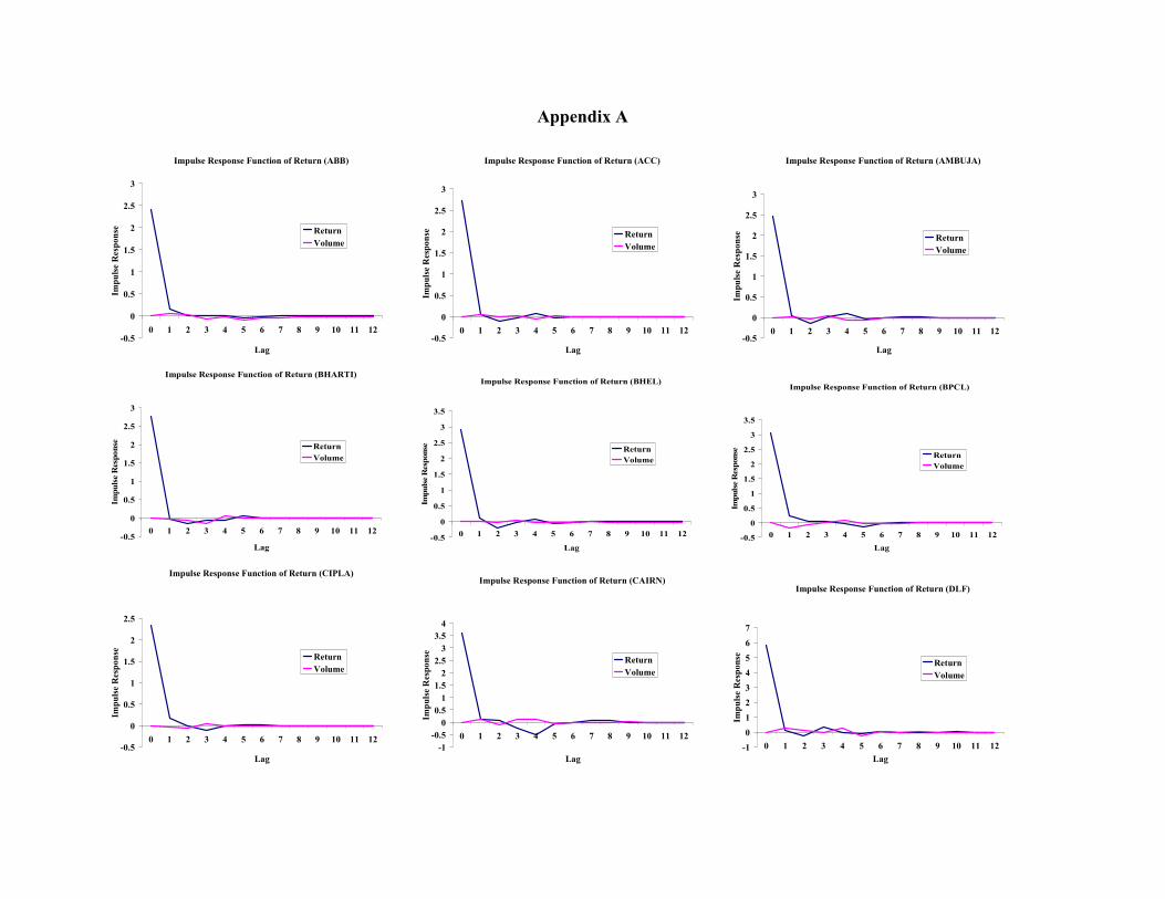
Appendix A
Impulse Response Function of Return (ABB)
-0.5
0
0.5
1
1.5
2
2.5
3
0 1 2 3 4 5 6 7 8 9 10 11 12
Lag
Impulse R
esp
onse Return
Volume
Impulse Response Function of Return (ACC)
-0.5
0
0.5
1
1.5
2
2.5
3
0 1 2 3 4 5 6 7 8 9 10 11 12
Lag
Impuls
e R
esp
onse Return
Volume
Impulse Response Function of Return (AMBUJA)
-0.5
0
0.5
1
1.5
2
2.5
3
0 1 2 3 4 5 6 7 8 9 10 11 12
Lag
Impulse R
esponse Return
Volume
Impulse Response Function of Return (BHARTI)
-0.5
0
0.5
1
1.5
2
2.5
3
0 1 2 3 4 5 6 7 8 9 10 11 12
Lag
Impulse R
esponse Return
Volume
Impulse Response Function of Return (BHEL)
-0.5
0
0.5
1
1.5
2
2.5
3
3.5
0 1 2 3 4 5 6 7 8 9 10 11 12
Lag
Impulse Res
ponse Return
Volume
Impulse Response Function of Return (BPCL)
-0.5
0
0.5
1
1.5
2
2.5
3
3.5
0 1 2 3 4 5 6 7 8 9 10 11 12
Lag
Impulse Res
ponse Return
Volume
Impulse Response Function of Return (CIPLA)
-0.5
0
0.5
1
1.5
2
2.5
0 1 2 3 4 5 6 7 8 9 10 11 12
Lag
Impulse R
esp
onse
Return
Volume
Impulse Response Function of Return (CAIRN)
-1
-0.5
0
0.5
1
1.5
2
2.5
3
3.5
4
0 1 2 3 4 5 6 7 8 9 10 11 12
Lag
Impuls
e R
esp
onse
Return
Volume
Impulse Response Function of Return (DLF)
-1
0
1
2
3
4
5
6
7
0 1 2 3 4 5 6 7 8 9 10 11 12
Lag
Impulse R
esp
onse
Return
Volume
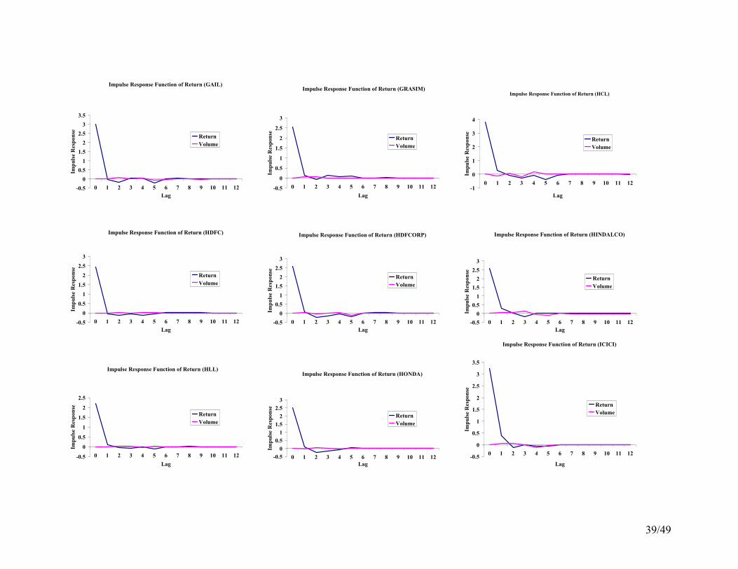
39/49
Impulse Response Function of Return (GAIL)
-0.5
0
0.5
1
1.5
2
2.5
3
3.5
0 1 2 3 4 5 6 7 8 9 10 11 12
Lag
Impuls
e R
esp
onse
Return
Volume
Impulse Response Function of Return (GRASIM)
-0.5
0
0.5
1
1.5
2
2.5
3
0 1 2 3 4 5 6 7 8 9 10 11 12
Lag
Impuls
e R
esp
onse
Return
Volume
Impulse Response Function of Return (HCL)
-1
0
1
2
3
4
0 1 2 3 4 5 6 7 8 9 10 11 12
Lag
Impulse R
esp
onse
Return
Volume
Impulse Response Function of Return (HDFC)
-0.5
0
0.5
1
1.5
2
2.5
3
0 1 2 3 4 5 6 7 8 9 10 11 12
Lag
Impulse R
esp
onse
Return
Volume
Impulse Response Function of Return (HDFCORP)
-0.5
0
0.5
1
1.5
2
2.5
3
0 1 2 3 4 5 6 7 8 9 10 11 12
Lag
Impulse R
esp
onse
Return
Volume
Impulse Response Function of Return (HINDALCO)
-0.5
0
0.5
1
1.5
2
2.5
3
0 1 2 3 4 5 6 7 8 9 10 11 12
Lag
Impulse R
esponse
Return
Volume
Impulse Response Function of Return (HLL)
-0.5
0
0.5
1
1.5
2
2.5
0 1 2 3 4 5 6 7 8 9 10 11 12
Lag
Impulse R
esp
onse
Return
Volume
Impulse Response Function of Return (HONDA)
-0.5
0
0.5
1
1.5
2
2.5
3
0 1 2 3 4 5 6 7 8 9 10 11 12
Lag
Impuls
e R
esp
onse
Return
Volume
Impulse Response Function of Return (ICICI)
-0.5
0
0.5
1
1.5
2
2.5
3
3.5
0 1 2 3 4 5 6 7 8 9 10 11 12
LagIm
puls
e R
esp
onse
Return
Volume
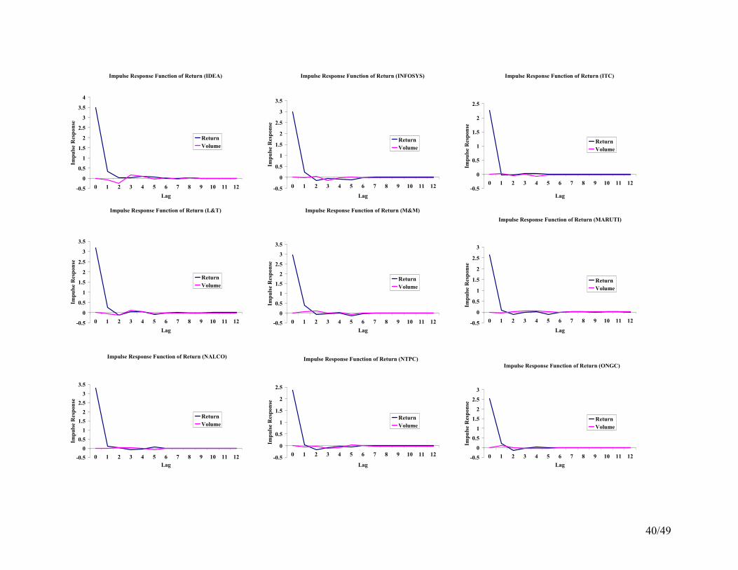
40/49
Impulse Response Function of Return (IDEA)
-0.5
0
0.5
1
1.5
2
2.5
3
3.5
4
0 1 2 3 4 5 6 7 8 9 10 11 12
Lag
Impulse R
esponse
Return
Volume
Impulse Response Function of Return (INFOSYS)
-0.5
0
0.5
1
1.5
2
2.5
3
3.5
0 1 2 3 4 5 6 7 8 9 10 11 12
Lag
Impulse R
esp
onse
Return
Volume
Impulse Response Function of Return (ITC)
-0.5
0
0.5
1
1.5
2
2.5
0 1 2 3 4 5 6 7 8 9 10 11 12
Lag
Impulse R
esp
onse
Return
Volume
Impulse Response Function of Return (L&T)
-0.5
0
0.5
1
1.5
2
2.5
3
3.5
0 1 2 3 4 5 6 7 8 9 10 11 12
Lag
Impulse R
esp
onse
Return
Volume
Impulse Response Function of Return (M&M)
-0.5
0
0.5
1
1.5
2
2.5
3
3.5
0 1 2 3 4 5 6 7 8 9 10 11 12
Lag
Impuls
e R
esp
onse
Return
Volume
Impulse Response Function of Return (MARUTI)
-0.5
0
0.5
1
1.5
2
2.5
3
0 1 2 3 4 5 6 7 8 9 10 11 12
Lag
Impulse R
esp
onse
Return
Volume
Impulse Response Function of Return (NALCO)
-0.5
0
0.5
1
1.5
2
2.5
3
3.5
0 1 2 3 4 5 6 7 8 9 10 11 12
Lag
Impuls
e R
esp
onse
Return
Volume
Impulse Response Function of Return (NTPC)
-0.5
0
0.5
1
1.5
2
2.5
0 1 2 3 4 5 6 7 8 9 10 11 12
Lag
Impuls
e R
esp
onse
Return
Volume
Impulse Response Function of Return (ONGC)
-0.5
0
0.5
1
1.5
2
2.5
3
0 1 2 3 4 5 6 7 8 9 10 11 12
LagIm
pulse R
esponse
Return
Volume
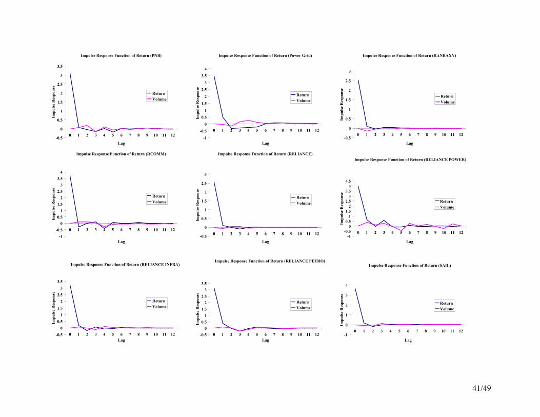
41/49
Impulse Response Function of Return (PNB)
-0.5
0
0.5
1
1.5
2
2.5
3
3.5
0 1 2 3 4 5 6 7 8 9 10 11 12
Lag
Impulse R
esp
onse
Return
Volume
Impulse Response Function of Return (Power Grid)
-1
-0.5
0
0.5
1
1.5
2
2.5
3
3.5
4
0 1 2 3 4 5 6 7 8 9 10 11 12
Lag
Impuls
e R
esp
onse
Return
Volume
Impulse Response Function of Return (RANBAXY)
-0.5
0
0.5
1
1.5
2
2.5
3
0 1 2 3 4 5 6 7 8 9 10 11 12
Lag
Impulse R
esponse
Return
Volume
Impulse Response Function of Return (RCOMM)
-1
-0.5
0
0.5
1
1.5
2
2.5
3
3.5
4
0 1 2 3 4 5 6 7 8 9 10 11 12
Lag
Impulse R
esp
onse
Return
Volume
Impulse Response Function of Return (RELIANCE)
-0.5
0
0.5
1
1.5
2
2.5
3
0 1 2 3 4 5 6 7 8 9 10 11 12
Lag
Impulse R
esp
onse
Return
Volume
Impulse Response Function of Return (RELIANCE POWER)
-1
-0.5
0
0.5
1
1.5
2
2.5
3
3.5
4
4.5
0 1 2 3 4 5 6 7 8 9 10 11 12
Lag
Impuls
e R
esp
onse
Return
Volume
Impulse Response Function of Return (RELIANCE INFRA)
-0.5
0
0.5
1
1.5
2
2.5
3
3.5
0 1 2 3 4 5 6 7 8 9 10 11 12
Lag
Impuls
e R
esp
onse
Return
Volume
Impulse Response Function of Return (RELIANCE PETRO)
-0.5
0
0.5
1
1.5
2
2.5
3
3.5
0 1 2 3 4 5 6 7 8 9 10 11 12
Lag
Impulse R
esp
onse
Return
Volume
Impulse Response Function of Return (SAIL)
-1
0
1
2
3
4
0 1 2 3 4 5 6 7 8 9 10 11 12
LagIm
puls
e R
esponse
Return
Volume
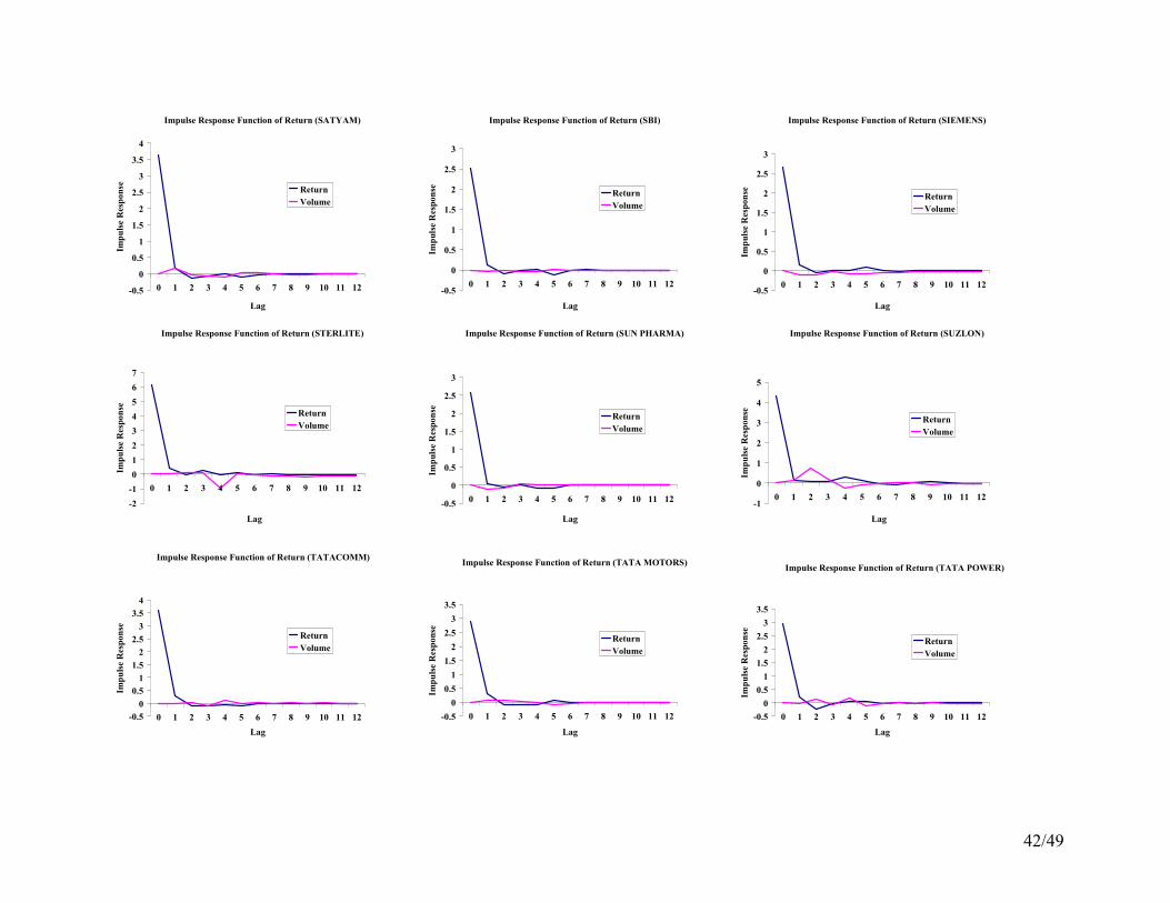
42/49
Impulse Response Function of Return (SATYAM)
-0.5
0
0.5
1
1.5
2
2.5
3
3.5
4
0 1 2 3 4 5 6 7 8 9 10 11 12
Lag
Impulse R
esp
onse Return
Volume
Impulse Response Function of Return (SBI)
-0.5
0
0.5
1
1.5
2
2.5
3
0 1 2 3 4 5 6 7 8 9 10 11 12
Lag
Impuls
e R
esp
onse Return
Volume
Impulse Response Function of Return (SIEMENS)
-0.5
0
0.5
1
1.5
2
2.5
3
0 1 2 3 4 5 6 7 8 9 10 11 12
Lag
Impuls
e R
esp
onse
Return
Volume
Impulse Response Function of Return (STERLITE)
-2
-1
0
1
2
3
4
5
6
7
0 1 2 3 4 5 6 7 8 9 10 11 12
Lag
Impulse R
esp
onse
Return
Volume
Impulse Response Function of Return (SUN PHARMA)
-0.5
0
0.5
1
1.5
2
2.5
3
0 1 2 3 4 5 6 7 8 9 10 11 12
Lag
Impuls
e R
esp
onse
Return
Volume
Impulse Response Function of Return (SUZLON)
-1
0
1
2
3
4
5
0 1 2 3 4 5 6 7 8 9 10 11 12
Lag
Impulse R
esp
onse
Return
Volume
Impulse Response Function of Return (TATACOMM)
-0.5
0
0.5
1
1.5
2
2.5
3
3.5
4
0 1 2 3 4 5 6 7 8 9 10 11 12
Lag
Impulse R
esp
onse
Return
Volume
Impulse Response Function of Return (TATA MOTORS)
-0.5
0
0.5
1
1.5
2
2.5
3
3.5
0 1 2 3 4 5 6 7 8 9 10 11 12
Lag
Impulse R
esp
onse
Return
Volume
Impulse Response Function of Return (TATA POWER)
-0.5
0
0.5
1
1.5
2
2.5
3
3.5
0 1 2 3 4 5 6 7 8 9 10 11 12
Lag
Impulse R
esp
onse
Return
Volume
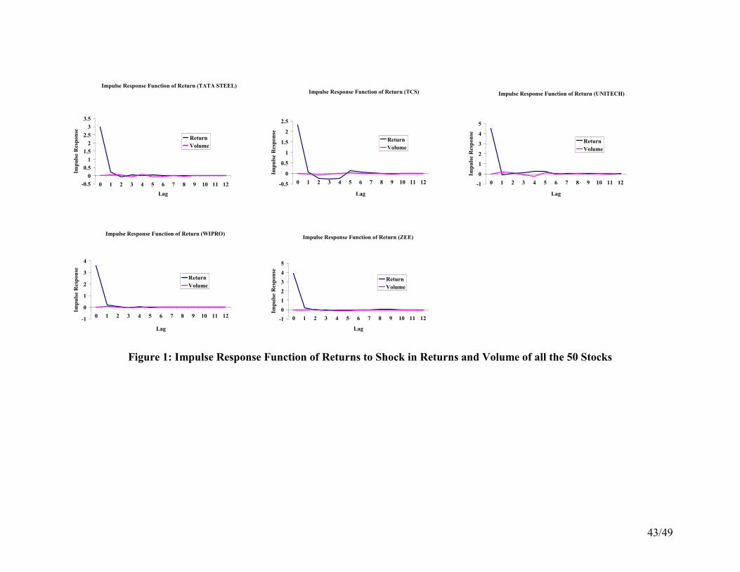
43/49
Impulse Response Function of Return (TATA STEEL)
-0.5
0
0.5
1
1.5
2
2.5
3
3.5
0 1 2 3 4 5 6 7 8 9 10 11 12
Lag
Impuls
e R
esp
onse
Return
Volume
Impulse Response Function of Return (TCS)
-0.5
0
0.5
1
1.5
2
2.5
0 1 2 3 4 5 6 7 8 9 10 11 12
Lag
Impulse R
esp
onse
Return
Volume
Impulse Response Function of Return (UNITECH)
-1
0
1
2
3
4
5
0 1 2 3 4 5 6 7 8 9 10 11 12
Lag
Impulse R
esp
onse
Return
Volume
Impulse Response Function of Return (WIPRO)
-1
0
1
2
3
4
0 1 2 3 4 5 6 7 8 9 10 11 12
Lag
Impuls
e R
esp
onse
Return
Volume
Impulse Response Function of Return (ZEE)
-1
0
1
2
3
4
5
0 1 2 3 4 5 6 7 8 9 10 11 12
Lag
Impulse R
esp
onse
Return
Volume
Figure 1: Impulse Response Function of Returns to Shock in Returns and Volume of all the 50 Stocks
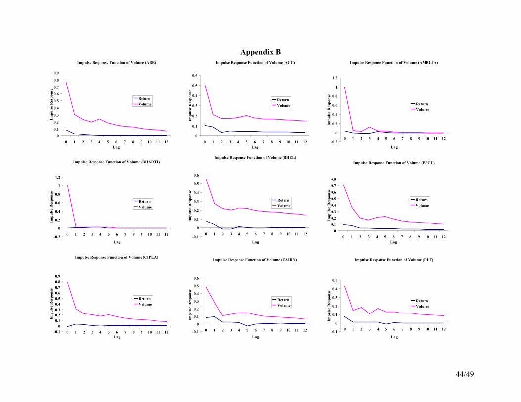
44/49
Appendix B
Impulse Response Function of Volume (ABB)
0
0.1
0.2
0.3
0.4
0.5
0.6
0.7
0.8
0.9
0 1 2 3 4 5 6 7 8 9 10 11 12
Lag
Impulse R
esp
onse
Return
Volume
Impulse Response Function of Volume (ACC)
0
0.1
0.2
0.3
0.4
0.5
0.6
0 1 2 3 4 5 6 7 8 9 10 11 12
Lag
Impulse R
esp
onse
Return
Volume
Impulse Response Function of Volume (AMBUJA)
-0.2
0
0.2
0.4
0.6
0.8
1
1.2
0 1 2 3 4 5 6 7 8 9 10 11 12
Lag
Impulse R
esponse
Return
Volume
Impulse Response Function of Volume (BHARTI)
-0.2
0
0.2
0.4
0.6
0.8
1
1.2
0 1 2 3 4 5 6 7 8 9 10 11 12
Lag
Impulse R
esp
onse
Return
Volume
Impulse Response Function of Volume (BHEL)
-0.1
0
0.1
0.2
0.3
0.4
0.5
0.6
0 1 2 3 4 5 6 7 8 9 10 11 12
Lag
Impulse R
esp
onse
Return
Volume
Impulse Response Function of Volume (BPCL)
0
0.1
0.2
0.3
0.4
0.5
0.6
0.7
0.8
0 1 2 3 4 5 6 7 8 9 10 11 12
Lag
Impulse R
esp
onse
Return
Volume
Impulse Response Function of Volume (CIPLA)
-0.1
0
0.1
0.2
0.3
0.4
0.5
0.6
0.7
0.8
0.9
0 1 2 3 4 5 6 7 8 9 10 11 12
Lag
Impuls
e R
esp
onse
Return
Volume
Impulse Response Function of Volume (CAIRN)
-0.1
0
0.1
0.2
0.3
0.4
0.5
0.6
0 1 2 3 4 5 6 7 8 9 10 11 12
Lag
Impulse R
esp
onse
Return
Volume
Impulse Response Function of Volume (DLF)
-0.1
0
0.1
0.2
0.3
0.4
0.5
0 1 2 3 4 5 6 7 8 9 10 11 12
Lag
Impuls
e R
esp
onse
Return
Volume
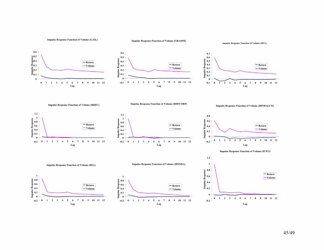
45/49
Impulse Response Function of Volume (GAIL)
0
0.1
0.2
0.3
0.4
0.5
0.6
0 1 2 3 4 5 6 7 8 9 10 11 12
Lag
Impulse R
esp
onse
Return
Volume
Impulse Response Function of Volume (GRASIM)
-0.1
0
0.1
0.2
0.3
0.4
0.5
0.6
0 1 2 3 4 5 6 7 8 9 10 11 12
Lag
Impulse R
esponse
Return
Volume
Impulse Response Function of Volume (HCL)
-0.1
0
0.1
0.2
0.3
0.4
0.5
0.6
0.7
0 1 2 3 4 5 6 7 8 9 10 11 12
Lag
Impulse R
esp
onse
Return
Volume
Impulse Response Function of Volume (HDFC)
-0.2
0
0.2
0.4
0.6
0.8
1
1.2
0 1 2 3 4 5 6 7 8 9 10 11 12
Lag
Impuls
e R
esp
onse
Return
Volume
Impulse Response Function of Volume (HDFCORP)
-0.2
0
0.2
0.4
0.6
0.8
1
1.2
0 1 2 3 4 5 6 7 8 9 10 11 12
Lag
Impulse R
esp
onse
Return
Volume
Impulse Response Function of Volume (HINDALCO)
-0.2
0
0.2
0.4
0.6
0.8
0 1 2 3 4 5 6 7 8 9 10 11 12
Lag
Impulse
Res
ponse
Return
Volume
Impulse Response Function of Volume (HLL)
-0.2
0
0.2
0.4
0.6
0.8
1
0 1 2 3 4 5 6 7 8 9 10 11 12
Lag
Impulse R
esp
onse
Return
Volume
Impulse Response Function of Volume (HONDA)
-0.2
0
0.2
0.4
0.6
0.8
1
0 1 2 3 4 5 6 7 8 9 10 11 12
Lag
Impulse R
esp
onse
Return
Volume
Impulse Response Function of Volume (ICICI)
-0.2
0
0.2
0.4
0.6
0.8
1
1.2
0 1 2 3 4 5 6 7 8 9 10 11 12
LagIm
pulse R
esp
onse
Return
Volume
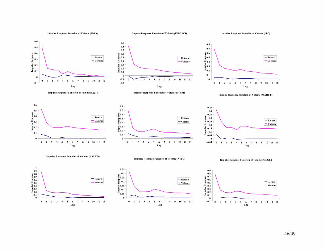
46/49
Impulse Response Function of Volume (IDEA)
-0.1
0
0.1
0.2
0.3
0.4
0.5
0.6
0 1 2 3 4 5 6 7 8 9 10 11 12
Lag
Impuls
e R
esp
onse
Return
Volume
Impulse Response Function of Volume (INFOSYS)
-0.2
-0.1
0
0.1
0.2
0.3
0.4
0.5
0.6
0.7
0.8
0.9
0 1 2 3 4 5 6 7 8 9 10 11 12
Lag
Impulse R
esponse
Return
Volume
Impulse Response Function of Volume (ITC)
0
0.1
0.2
0.3
0.4
0.5
0.6
0.7
0.8
0 1 2 3 4 5 6 7 8 9 10 11 12
Lag
Impuls
e R
esp
onse
Return
Volume
Impulse Response Function of Volume (L&T)
0
0.1
0.2
0.3
0.4
0.5
0.6
0 1 2 3 4 5 6 7 8 9 10 11 12
Lag
Impulse R
esponse
Return
Volume
Impulse Response Function of Volume (M&M)
0
0.1
0.2
0.3
0.4
0.5
0.6
0.7
0.8
0 1 2 3 4 5 6 7 8 9 10 11 12
Lag
Impulse R
esp
onse
Return
Volume
Impulse Response Function of Volume (MARUTI)
-0.05
0
0.05
0.1
0.15
0.2
0.25
0.3
0.35
0.4
0.45
0 1 2 3 4 5 6 7 8 9 10 11 12
Lag
Impuls
e R
esp
onse
Return
Volume
Impulse Response Function of Volume (NALCO)
0
0.1
0.2
0.3
0.4
0.5
0.6
0.7
0.8
0.9
1
0 1 2 3 4 5 6 7 8 9 10 11 12
Lag
Impuls
e R
esp
onse
Return
Volume
Impulse Response Function of Volume (NTPC)
0
0.05
0.1
0.15
0.2
0.25
0.3
0.35
0 1 2 3 4 5 6 7 8 9 10 11 12
Lag
Impulse R
esp
onse
Return
Volume
Impulse Response Function of Volume (ONGC)
-0.1
0
0.1
0.2
0.3
0.4
0.5
0.6
0.7
0.8
0.9
0 1 2 3 4 5 6 7 8 9 10 11 12Lag
Impulse R
esp
onse
Return
Volume
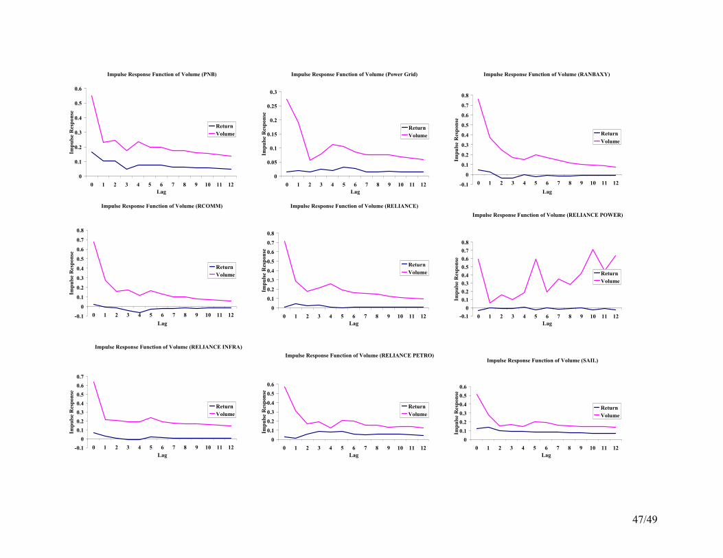
47/49
Impulse Response Function of Volume (PNB)
0
0.1
0.2
0.3
0.4
0.5
0.6
0 1 2 3 4 5 6 7 8 9 10 11 12
Lag
Impulse R
esp
onse
Return
Volume
Impulse Response Function of Volume (Power Grid)
0
0.05
0.1
0.15
0.2
0.25
0.3
0 1 2 3 4 5 6 7 8 9 10 11 12
Lag
Impulse R
esp
onse
Return
Volume
Impulse Response Function of Volume (RANBAXY)
-0.1
0
0.1
0.2
0.3
0.4
0.5
0.6
0.7
0.8
0 1 2 3 4 5 6 7 8 9 10 11 12
Lag
Impulse R
esponse
Return
Volume
Impulse Response Function of Volume (RCOMM)
-0.1
0
0.1
0.2
0.3
0.4
0.5
0.6
0.7
0.8
0 1 2 3 4 5 6 7 8 9 10 11 12
Lag
Impulse R
esp
onse
Return
Volume
Impulse Response Function of Volume (RELIANCE)
0
0.1
0.2
0.3
0.4
0.5
0.6
0.7
0.8
0 1 2 3 4 5 6 7 8 9 10 11 12
Lag
Impulse R
esponse
Return
Volume
Impulse Response Function of Volume (RELIANCE POWER)
-0.1
0
0.1
0.2
0.3
0.4
0.5
0.6
0.7
0.8
0 1 2 3 4 5 6 7 8 9 10 11 12
Lag
Impuls
e R
esp
onse
Return
Volume
Impulse Response Function of Volume (RELIANCE INFRA)
-0.1
0
0.1
0.2
0.3
0.4
0.5
0.6
0.7
0 1 2 3 4 5 6 7 8 9 10 11 12
Lag
Impuls
e R
esp
onse
Return
Volume
Impulse Response Function of Volume (RELIANCE PETRO)
0
0.1
0.2
0.3
0.4
0.5
0.6
0 1 2 3 4 5 6 7 8 9 10 11 12
Lag
Impulse R
esp
onse
Return
Volume
Impulse Response Function of Volume (SAIL)
0
0.1
0.2
0.3
0.4
0.5
0.6
0 1 2 3 4 5 6 7 8 9 10 11 12
LagIm
pulse R
esp
onse
Return
Volume
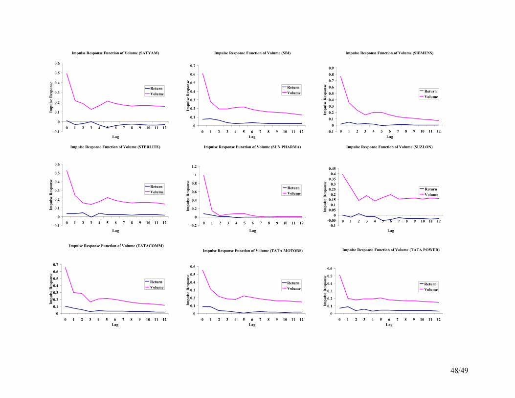
48/49
Impulse Response Function of Volume (SATYAM)
-0.1
0
0.1
0.2
0.3
0.4
0.5
0.6
0 1 2 3 4 5 6 7 8 9 10 11 12
Lag
Impulse R
esp
onse
Return
Volume
Impulse Response Function of Volume (SBI)
0
0.1
0.2
0.3
0.4
0.5
0.6
0.7
0 1 2 3 4 5 6 7 8 9 10 11 12
Lag
Impuls
e R
esponse
Return
Volume
Impulse Response Function of Volume (SIEMENS)
-0.1
0
0.1
0.2
0.3
0.4
0.5
0.6
0.7
0.8
0.9
0 1 2 3 4 5 6 7 8 9 10 11 12
Lag
Impulse R
esp
onse
Return
Volume
Impulse Response Function of Volume (STERLITE)
-0.1
0
0.1
0.2
0.3
0.4
0.5
0.6
0 1 2 3 4 5 6 7 8 9 10 11 12
Lag
Impulse R
esp
onse
Return
Volume
Impulse Response Function of Volume (SUN PHARMA)
-0.2
0
0.2
0.4
0.6
0.8
1
1.2
0 1 2 3 4 5 6 7 8 9 10 11 12
Lag
Impulse R
esp
onse
Return
Volume
Impulse Response Function of Volume (SUZLON)
-0.1
-0.05
0
0.05
0.1
0.15
0.2
0.25
0.3
0.35
0.4
0.45
0 1 2 3 4 5 6 7 8 9 10 11 12
Lag
Impulse R
esp
onse
Return
Volume
Impulse Response Function of Volume (TATACOMM)
0
0.1
0.2
0.3
0.4
0.5
0.6
0.7
0 1 2 3 4 5 6 7 8 9 10 11 12
Lag
Impuls
e R
esp
onse
Return
Volume
Impulse Response Function of Volume (TATA MOTORS)
0
0.1
0.2
0.3
0.4
0.5
0.6
0 1 2 3 4 5 6 7 8 9 10 11 12
Lag
Impulse R
esp
onse
Return
Volume
Impulse Response Function of Volume (TATA POWER)
0
0.1
0.2
0.3
0.4
0.5
0.6
0 1 2 3 4 5 6 7 8 9 10 11 12
LagIm
puls
e R
esp
onse
Return
Volume
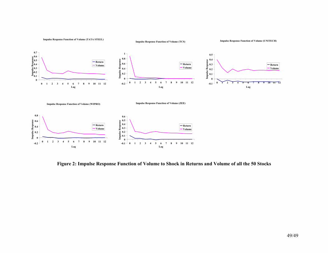
49/49
Impulse Response Function of Volume (TATA STEEL)
0
0.1
0.2
0.3
0.4
0.5
0.6
0.7
0 1 2 3 4 5 6 7 8 9 10 11 12
Lag
Impuls
e R
esponse
Return
Volume
Impulse Response Function of Volume (TCS)
-0.2
0
0.2
0.4
0.6
0.8
1
0 1 2 3 4 5 6 7 8 9 10 11 12
Lag
Impulse R
esponse
Return
Volume
Impulse Response Function of Volume (UNITECH)
-0.1
0
0.1
0.2
0.3
0.4
0.5
0 1 2 3 4 5 6 7 8 9 10 11 12
Lag
Impulse R
esponse
Return
Volume
Impulse Response Function of Volume (WIPRO)
-0.2
0
0.2
0.4
0.6
0.8
0 1 2 3 4 5 6 7 8 9 10 11 12
Lag
Impulse R
esp
onse
Return
Volume
Impulse Response Function of Volume (ZEE)
-0.1
0
0.1
0.2
0.3
0.4
0.5
0.6
0 1 2 3 4 5 6 7 8 9 10 11 12
Lag
Impulse R
esponse
Return
Volume
Figure 2: Impulse Response Function of Volume to Shock in Returns and Volume of all the 50 Stocks