Seediscussions,stats,andauthorprofilesforthispublicationat:https://www.researchgate.net/publication/278159272

TheDynamicEffectsofChangesinPricesandAffordabilityonAlcoholConsumption:AnImpulseResponseAnalysis

ArticleinAlcoholandAlcoholism·June2015

DOI:10.1093/alcalc/agv064·Source:PubMed

CITATIONS

4

READS

104

2authors:

HengJiang

LaTrobeUniversity

30PUBLICATIONS56CITATIONS

SEEPROFILE

MichaelJohnLivingston

LaTrobeUniversity

117PUBLICATIONS1,652CITATIONS

SEEPROFILE

AllcontentfollowingthispagewasuploadedbyHengJiangon29June2015.

Theuserhasrequestedenhancementofthedownloadedfile.Allin-textreferencesunderlinedinblueareaddedtotheoriginaldocumentandarelinkedtopublicationsonResearchGate,lettingyouaccessandreadthemimmediately.

1

The dynamic effects of changes in prices and affordability on alcohol

consumption: an impulse response analysis

Heng Jiang 1, 2, *

, Michael Livingston

1, 3

1 Centre for Alcohol Policy Research, Turning Point, Melbourne, Victoria, Australia

2 Eastern Health Clinical School, Monash University, Melbourne, Victoria, Australia

3 Drug Policy Modelling Program, National Drug and Alcohol Research Centre, The

University of New South Wales, New South Wales, Australia

Running title: Alcohol price and affordability on consumption

Total page count: 14

Word count for abstract: 241

Word count for body text: 3513

References: 28

Tables: 0

Figures: 6

*Corresponding address: Heng Jiang,

Centre for Alcohol Policy Research, Turning Point, 54 Gertrude

Street, Fitzroy, VIC, 3065,

E-mail: jasonj@turningpoint.org.au

P: 03 84138452

F: 03 94163420

2

Abstract

Aims: To investigate how changes in alcohol price and affordability are related to aggregate

level alcohol consumption in Australia to help to inform effective price and tax policy to

influence consumption.

Material and methods: Annual time series data between 1974 and 2012 on price and per-

capita consumption for beer, wine and spirits and average weekly income were collected

from the Australian Bureau of Statistics. Using a Vector Autoregressive model and impulse

response analysis, the dynamic responses of alcohol consumption to changes in alcohol prices

and affordability were estimated.

Results: Alcohol consumption in Australia was negatively associated with alcohol price and

positively associated with the affordability of alcohol. The results of the impulse response

analysis suggest that a 10% increase in the alcohol price was associated with a 2% decrease

in the population-level alcohol consumption in the following year, with further, diminishing,

effects up to year 8, leading to an overall 6% reduction in total consumption. In contrast,

when alcohol affordability increased, per capita alcohol consumption increased over the

following 6 years.

Conclusions: Our findings suggest that increasing alcohol prices or taxes can help to reduce

alcohol consumption at the population level in Australia. However, the impact of

affordability in our findings highlights that pricing policies need to consider increases in

income to ensure effectiveness. Alcohol price policy should only cautiously focus on

individual beverage types, because increasing the price of one beverage generally leads to an

increase in consumption of substitutes.

Key words: Alcohol price, affordability, price policy, VAR model, impulse response

3

INTRODUCTION

Preventing and reducing the health and social burden caused by the harmful use of alcohol

has become a public health priority and one of the objectives of the World Health

Organization (WHO) (2014). Policies that increase alcohol tax or retail prices are regarded as

one of the most effective means to reduce population level alcohol consumption and related

harm (Anderson et al., 2009). Studies examining the impact of price on consumption

generally talk about the price elasticity of a commodity – that is, the relative reduction in

consumption for a unit increase in price. If a 10% increase in price leads to a 10% reduction

in consumption, then the price elasticity is -1. Using this measure, a number of systematic

reviews have shown that the mean price elasticity of demand is -0.4 for beer, -0.7 for wine, -

0.7 for spirits and for overall, the response of alcohol consumption to changes of alcohol

price is estimated at approximately -0.5 (Gallet, 2007; Wagenaar et al., 2009; Fogarty, 2010).

This elasticity implies that a 10% rise in alcohol price will be expected to decrease the overall

demand for alcohol by about 5%. However, the price elasticity of alcohol demand varies

substantially depending on drinking culture, economic conditions and across different

beverages, which may have different social meanings and roles (Zhang and Casswell, 1999).

The meta-analyses described above summarise a significant literature on the price elasticity

of alcohol demand, but much of this research has focused on just the own-price elasticity of

beverages (own-price elasticity measures the responsiveness of demand for a good to a

change in its own price and cross-price elasticity measures the responsiveness of the demand

for a good to a change in the price of another good). As the prices and taxes for difference

types of alcohol are different in many countries (e.g. U.K., U.S., Australia, New Zealand and

etc.) and consumers may respond to price rises by shifting brand or beverage (Gruenewald et

al., 2006), estimating both own-price and cross-price elasticities is very important. The

4

estimation of cross-price elasticities can help to identify whether there are substitute or

complement relationships between two types of alcohol beverages (Meng et al., 2014),

providing clearer evidence on the likely changes in consumption following particular tax or

price changes. A substitute is something that can be used instead of a particular good or

service, and a complement is an item that can be used in conjunction with one another. In this

instance if, for example, beer and wine were substitutes then an increase in beer prices and

corresponding decrease in beer consumption may be offset by an increase in wine

consumption. If they were complements, then a beer tax increase would reduce both beer and

wine consumption.

Income or affordability has also been shown to be a significant factor that can affect alcohol

consumption. When income increases, alcohol consumption may increase as alcohol products

become more affordable for consumers (Gallet, 2007; Nelson, 2013). A study in European

countries found that alcohol beverages have become more affordable in most European

countries since the mid-1990s, with positive relationships found between affordability and

alcohol consumption and related harms (Rabinovich et al., 2009). Based on a time series

analysis, Wall and Casswell (2013) found that affordability had a stronger association with

demand for alcohol than the real price in New Zealand and suggested that alcohol

affordability is an important parameter to be considered in alcohol price or taxation policy. If

the income index increases faster than the real alcohol price index, then alcohol beverages

will become more affordable for consumers.

There has been some previous analyses of price and income elasticities of alcohol in

Australia, the price and income elasticities of demand for alcohol have been examined in a

number of studies (Haque, 1990; Clements and Selvanathan, 1991; Selvanathan and

5

Selvanathan, 2004; Fogarty, 2010). In an aggregate study of data between 1956 and 1999,

(Selvanathan and Selvanathan, 2004) found that income and prices were significantly related

to the consumption patterns of alcohol in Australia with the mean price and income

elasticities of -0.61 and 0.72 respectively. Based on panel survey data, Sharma et al. (2014)

estimated price elasticities of -0.49 for beer, -0.53 for wine and -1.28 for spirits in Victoria.

Using time series data from 1955 to 1986, Clements and Selvanathan (1991) reported that

own-price elasticity was -0.15 for beer, -0.32 for wine and -0.61 for spirits while income

elasticity was 0.73 for beer, 0.61 for wine and 2.51 for spirits.

The studies discussed above and reviewed in the cited meta-analyses have examined the

relationships between price, affordability and demand for alcohol using individual or

aggregate data, and by various methods (e.g. linear regression, autoregressive integrated

moving average model, panel data regression, survey analysis etc. (Clements and

Selvanathan, 1991; Gallet, 2007; Fogarty, 2010; Sharma et al., 2014). However, none of them

have explored the dynamic temporal effects of changes in price and affordability on alcohol

demand, e.g. if the alcohol price or affordability increases 10%, what are the immediate and

lagged effects on alcohol consumption and how long do the effects last. Changes in price will

have an immediate effect on consumption, but there is a potential for these effects to be

spread over time. For example, studies in the housing market have shown that a 10% increase

in interest rates will lead to a dynamic change in housing starts or demand over time – an

overall 12% decrease in following 10 quarters (Berger-Thomson and Ellis, 2004). In this

case, we explore whether there are longer-term effects of price and affordability changes and

how these effects are distributed over time using advanced econometric analysis techniques,

namely, vector autoregressive (VAR) model and impulse response analysis.

6

METHODS

Data

All time series data were collected from Australian Bureau of Statistics (ABS). Annual per

capita alcohol and beverage-specific (beer, wine and spirits) consumption in litres of pure

alcohol were obtained for 1974 to 2012 (age 15+) – were used as the measures of demand for

alcohol overall and for each of the three beverages (Australian Bureau of Statistics, 2013a).

A measure of price was estimated using data from the Consumer Price Index. A real alcohol

price index can be computed as: real alcohol or beverage-specific price indices = alcohol or

beverage-specific CPIs / all goods CPI (Seabrook, 2010). This method adjusts for inflation

and reflects the price of alcohol relative to all other consumable goods (Wall and Casswell,

2013). Quarterly alcohol and beer CPIs are available since 1974; CPI series for spirits and

wine both start in 1980 (Australian Bureau of Statistics, 2014). Quarterly time series were all

averaged to annual data for the analysis.

An alcohol affordability index was calculated, defined as the average income index divided

by real alcohol price index. The average weekly earnings from 1974 was used as the baseline

for the income index. The survey of average weekly earnings is used to measure the level of

average gross weekly earnings associated with employees in Australia, but does not capture

all the information about the distribution (Australian Bureau of Statistics, 2013c; 2013b).

Econometric estimating techniques

Vector autoregressive models and impulse response analyses were employed to estimate the

dynamic response of overall alcohol demand to changes in price and affordability. Further

models were developed for specific beverages, assessing the impact of changes either in its

7

own price and affordability or in other beverages’ prices and affordability. The VAR model,

developed by Sims (1980) in 1980, is one of the most applied models in time series analysis.

Stationary series with time trends removed reduce the risk of obtaining a spurious estimation

(George, 1994). In most cases, a differencing of the time series is sufficient to eliminate non-

stationarity. The Augmented Dickey-Fuller (ADF) unit root test, developed by Dickey and

Fuller was employed to test stationarity for the time series (Dickey and Fuller, 1979).

Differencing of time-series data also helps to minimise the risk of unmeasured confounding

(Norström, 2001).

Specifically the VAR models for alcohol demand ( ) can be presented as follows,

where is per capita alcohol consumption at time t, is the lagged per capita alcohol

consumption, represent alcohol price or affordability indices, is first difference of

the variables, k is the number of lags, represent the coefficients of independent variables,

C is the intercept, and the residuals. Estimates produced here are unconditional temporal

estimates. In this study, four key analyses were conducted: 1) response of alcohol

consumption to price change, 2) response of alcohol consumption to affordability change, 3)

responses of the consumption of the three specific beverage types to changes in beverage-

specific prices, and 4) responses of the consumption of the three beverage types to changes in

beverage-specific affordability.

The lag length is selected for a time series in VAR modelling on the basis of the sequential

modified likelihood ratio test statistic (LR), final prediction error (FPE), Akaike information

8

criterion (AIC), Schwarz information criterion (SC) and Hannan–Quinn information criterion

(HQ). The appropriate lag lengths for the alcohol and beverage-specific estimating models

were identified as one year. After establishing VAR models for demand for alcohol and the

three types of beverages, serial correlation Lagrange multiplier tests (LM), White’s

heteroskedasticity test (White) and Jarque–Bera normality tests (Jarque–Bera) were

conducted to verify the standard assumptions on residual correlation, heteroskedasticity and

normality respectively.

After the establishment of VAR model, the impulse response function can be conducted to

assess the dynamic impacts of price and affordability on alcohol demand in Australia. The

formulation and implementation of VAR model impulse response function were elaborated in

the study of Lütkepohl and Reimers (1992). The VAR impulse response function procedure

can be used to trace responses of a set of variables to shocks in another set of variables

(Hamilton, 1994). Impulse response functions are computed to give an indication of the

system's dynamic behaviour. It can indicate whether the impacts are positive or negative, or

whether these impacts are a temporary jump or indicate long-run persistence.

RESULTS

Between 1974 and 2012, the trends in real alcohol price and affordability indices and per

capita alcohol consumption are shown in Fig. 1. The indices of alcohol price and affordability

are set to equal 100 in 2010. Per capita alcohol consumption decreased gradually from 13 L

to 10 L between 1974 and 1992 and was then stable up to 2000. Between 2000 and 2006,

consumption increased again to about 11 L, and has dropped back to 10 L in the last 6 years.

The alcohol affordability index had similar fluctuations to per capita alcohol consumption in

the last 40 years. It can be observed that the alcohol affordability index decreased during the

9

1970s up to 1982 and had a small increase in 1983-84 and then remained as a same level after

1984. A possible reason for this increase in affordability is the introduction of an income tax-

free threshold in 1983-84, leading to an increase in average income. In contrast, the alcohol

price index increased steadily over the study period.

<Insert Figure 1 about here>

Fig. 2 shows the trend of total alcohol and beverage-specific consumption during 1974 and

2012. Per capita beer consumption decreased dramatically from 9 L to 4 L between 1974 and

2012, while per capita wine consumption increased steadily from 2 L to 4 L and per capita

spirits consumption increased slightly from 1.6 L to 2 L between 1980 and 2006 and

decreased to 1.8 L after 2006.

<Insert Figure 2 about here>

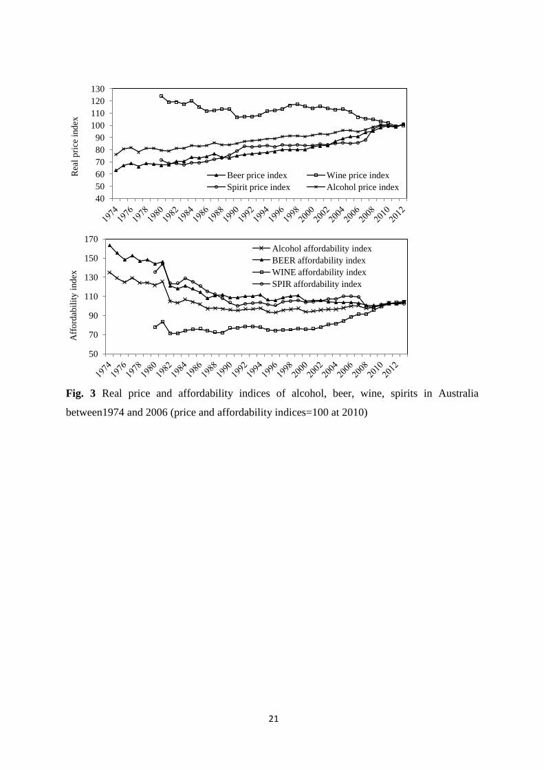
The fluctuations of the alcohol price and affordability indices are shown in Fig. 3 for beer,

wine and spirits. The wine price decreased from 1980 to 2012 and the affordability index of

wine increased significantly from 70 to 105. At the same time, beer and spirits price indices

both increased dramatically and their affordability indices decreased steadily during the study

period.

<Insert Figure 3 about here>

The stationarity of the selected time series was tested using the ADF tests and the results

suggest that all of the time series were stationary after first differencing I(1), (p<0.05). Based

10

on the VAR lag length selection system, the smallest values of the LR, FPE, AIC, SC, and

HQ tests indicate that the appropriate lag lengths for the alcohol and beverage-specific

estimating models were one year. Furthermore, all proposed models passed all validation

tests at the 5% significance level, indicating that there were no sigificant departures from the

standard assumptions for all VAR models, and the estimated coefficients were stable across

the sample period.

Impulse response analysis was then conducted to explore the short-term and long-term

temporal effects of changes in alcohol and beverage-specific prices and affordabilities on

alcohol and beverage-specific consumption level (results shown in Figs 4-6). Fig. 4 shows a

negative response from alcohol consumption to an increase in the alcohol price index and a

positive response to alcohol affordability, with time lags. These results indicate that if the

alcohol price increases 1% (or 10%) in one year, per capita alcohol consumption will

decrease by about 0. 2% (or 2%) in the second year, with effects becoming weaker in the

following years, and dissipating after the 8th

year. Overall, an increase of 10% in the alcohol

price will lead to a 6% accumulated reduction in per capita alcohol consumption over an 8-

year period. In contrast, if alcohol affodability increases 10%, per capita alcohol

consumption will increase by about 1% in the second year with weaker positive effects found

between the third and sixth years, leading to an overall 3% increase in per capita alcohol

consumption.

<Insert Figure 4 about here>

The responses of consumption to changes in beverage-specific prices over a 12-year period

are shown in Fig. 5. The results of impulse response analyses suggest that beer consumption

11

was negatively affected by increases in beer price, but was positively affected by the

increases in wine price, while an increase in spirits price would lead to a slight decrease in

beer consumption. Per capita wine consumption received very small impacts from the

changes in wine price and nearly no shock from the changes in beer price. However, wine

consumption was significantly and positively impacted by the increases in spirits price (a

10% increase in spirits price will lead to an accumulated 3% increase in per capita wine

consumption over 10 years). Spirits consumption was more sensitive to its own price change.

When spirits prices increased by 10%, spirits consumption decreased by 3% in the second

year, 2% in the third year and 1% in the fourth year with effects becoming weaker and

tending to disappear after the fourth year leading to an overall decline of 6%.

<Insert Figure 5 about here>

Fig. 6 shows the response of consumption of the three types of beverage to changes in

affordability. Beer consumption was positively associated with an increase in beer

affordability and negatively associated with an increase in wine affordability. The impact of

an increase in spirits affordability on beer consumption was moderate over the estimation

period. The results indicate that wine consumption level received very small impacts from

changes in affordabilities of wine, beer and spirits. Changes in spirits affordability had a

strong positive impact on spirits consumption at the population level (a 10% increase in

spirits affordability led to a 3% increase in per capita spirits consumption in the second year

and weaker increases in spirits consumption between the third and eighth years). However, an

increase in wine affordability led to a significant decrease in spirits consumption, with effects

spread across six years. It is worth noting that an increase in beer affordability was linked to

12

an increase in spirits consumption in the short-term, but in the long-term it was associated

with reduced spirits consumption.

<Insert Figure 6 about here>

DISCUSSION

This study has explored the dynamic responses of consumption levels to changes in prices

and affordabilities of alcohol overall and three types of beverages (e.g. beer, wine and spirits)

using over 30 years of time series data. The study findings suggest that a 10% increase in the

alcohol price was associated with a 2% reduction in per capita alcohol consumption in the

year after the price change and weaker reductions spread between the third and eighth years,

leading to an accumulated 6% reduction over an 8-year period (see Figure 4). In contrast, a

10% increase in alcohol affordability was associated with an increase in alcohol consumption

both in the short-term and long-term with overall 3% increases. A meta-analyses suggested

that the ratios of the percentage change in demand to the percentage change in alcohol price

under 2% are small, 5% are medium and over 8% are large (Wagenaar et al., 2009).

Compared with other studies, our estimates of price effectiveness sit slightly above the

middle of the broad literature, with a ratio of 6% change in total alcohol consumption,

suggesting that the manipulation of tax rates or prices can reduce the harms due to alcohol

consumption and achieve substantial health benefits in Australia.

Trends in beverage specific consumption are consistent with the trends in affordabilities of

beer, wine and spirits in the study period, e.g. beer consumption has steadily decreased in the

last 30 years and this may be linked to the continued inrease in beer price and decline in beer

affordability. The beverage-specific analyses suggest that wine consumption only received

13

moderate impact from the changes in prices and affordabilities of beer, wine and spirits.

However, the increase in wine affordability was linked to large reductions in beer and spirits

consumption, which may explain the long-term change in the preferences away from beer and

spirits towards wine in Australia. Compared with wine, per capita beer and spirits

consumption both received strong and negative impacts from the changes in prices of

themselves and other types of beverages. Changes in affordability of beer and spirits will lead

to siginificant impacts on the comsumption of all three beverages.

The Australian alcohol taxation system is complex, with tax rates varying between beverage

types and even container type. A particular issue is that beer and spirits are taxed on the basis

of alcohol content and wine on the basis of price, meaning that cheap wine (e.g. in casks) has

a very low level of tax associated with it (Vandenberg et al., 2008). Government policies

have tended to treat alcoholic beverages as independent, when there are complex links

between them. For example, the implementation of the alcopops tax in 2008 sharply reduced

alcopops consumption, but around half of this impact was offset by increases in the

consumption of spirits and other beverages (Chikritzhs et al., 2009). The results of the

beverage-specific impulse response analyses presented here suggest that alcohol price policy

should not focus on individual type of beverages, because of the complex substitute and

compliment relationships between beverages. Approaches that cover all beverages, such as

volumetric based taxation based on alcohol content are more likely to reduce alcohol

consumption and related harms (Sharma et al., 2014).

Additionally, our research findings highlight and confirm that raising alcohol prices or tax

can help to reduce alcohol consumption at the population level in Australia. Furthermore, the

results of temporal analsis reveal that when the price and affordability of alcohol changed,

14

consumption is affected for up to eight years (with the strongest effects immediately). This,

along with the positive effects on consumption seen for increased affordability, reinforces the

need for ongoing and regular review of the alcohol taxation system to ensure its effectiveness

as a public health measure.

While there have been many previous studies of the relationship between price, consumption

and affordability of alcohol (Gallet, 2007; Nelson, 2013), this study is the first study that

explores dynamic relationships between alcohol consumption, price and affordability in the

temporal dimension. This study is somewhat limited by its short time scale (39 years) and its

use of aggregate level data. This last fact in particular raises the issue of the ecological fallacy

and some care should be taken in applying these findings at the individual level. However,

the proposed models have passed all the validation tests, indicating that the estimates are

reliable and the aim of public health policies on alcohol prices is to reduce aggregate levels of

consumption. Furthermore, due to the data availability only three types of beverages were

estimated in proposed VAR models, and more sophisticated research on the cross-types

relationships between consumption on wider range of beverages (e.g. cider, Ready-To-Drink,

cask wine, and etc.), prices and affordabilities need to be conducted in the future.

Additionally, there are many other factors may affect alcohol consumption and we did not

include in the estimation, such as changes in economic conditions (e.g. GDP and

unemployment rates), changes in expenditure on other goods and necessities (e.g. housing

costs, fuel and tobacco price) and impacts of key alcohol policies (e.g. the introduction of

Random Breath Testing program in 1976-1980s etc.). However, as demonstrated by

Norström (2001), the use of differenced time-series data reduces the potential risk of

confounding, requiring a confounding variable to be correlated with annual changes in both

input (e.g. price) and output (e.g. alcohol consumption) series.

15

Acknowledgements

The research was funded by a project grant from the Australian National Health and Medical

Research Council (grant number #566629). The Centre for Alcohol Policy is funded by the

Foundation for Alcohol Research and Education (FARE), an independent, charitable

organisation working to prevent the harmful use of alcohol in Australia (www.fare.org.au).

ML is supported by a National Health and Medical Research Council Early Career

Fellowship.

Conflicts of Interest

Authors declare that we have no conflicts of interest.

16

References

Anderson P, Chisholm D, Fuhr DC. (2009) Effectiveness and cost-effectiveness of policies

and programmes to reduce the harm caused by alcohol, Lancet 373: 2234-2246.

Australian Bureau of Statistics (2013a), Apparent Consumption of Alcohol, Australia, 2012-

13, Cat. no. 4307.0.55.001, Australian Bureau of Statistics, Canberra, Australia.

Australian Bureau of Statistics (2013b), Average Weekly Earnings, Australia, Nov 2013 , Cat.

no. 6302.0, Australian Bureau of Statistics, Canberra, Australia.

Australian Bureau of Statistics (2013c), Employee Earnings, Benefits and Trade Union

Membership -- Cat. no. 6310.0, Australian Bureau of Statistics, Canberra, Australia.

Australian Bureau of Statistics (2014), Consumer Price Index, Australia, Jun 2014, Cat. no.

6401.0, Australian Bureau of Statistics, Canberra, Australia.

Berger-Thomson L, Ellis L (2004), Housing construction cycles and interest rates, Reserve

Bank of Australia, Canberra, Australia.

Chikritzhs T, Dietze P, Allsop S, Daube M, Hall W, Kypri K. (2009) The "alcopops" tax :

Heading in the right direction, Med J Aust 190: 294-295.

Clements KW, Selvanathan S. (1991) The economic determinants of alcohol consumption,

Australian Journal of Agricultural Economics 35: 209-231.

Dickey DA, Fuller WA. (1979) Distribution of the estimators for autoregressive time series

with a unit root, J Am Statist Assoc 74: 427-431.

Fogarty J. (2010) The demand for beer, wine and spirits: A survey of the literature, J Econ

Surv 24: 428-478.

Gallet CA. (2007) The demand for alcohol: a meta-analysis of elasticities, J Agr Resour Econ

51: 121-135.

George B (1994), Time Series Analysis: Forecasting & Control, 3rd Ed., Pearson Education,

17

Gruenewald PJ, Ponicki WR, Holder HD, Romelsjö A. (2006) Alcohol prices, beverage

quality, and the demand for alcohol: Quality substitutions and price elasticities,

Alcohol Clin Exp Res 30: 96-105.

Hamilton JD (1994), Time Series Analysis, Princeton University Press, Princeton.

Haque MO. (1990) The demand for alcohol in Australia, Drug Alcohol Rev 9: 43-52.

Lütkepohl H, Reimers H-E. (1992) Impulse response analysis of cointegrated systems, J

Econ Dyn Control 16: 53-78.

Meng Y, Brennan A, Purshouse R, Hill-McManus D, Angus C, Holmes J, Meier PS. (2014)

Estimation of own and cross price elasticities of alcohol demand in the UK—A

pseudo-panel approach using the Living Costs and Food Survey 2001–2009, J Health

Econ 34: 96-103.

Nelson J. (2013) Meta-analysis of alcohol price and income elasticities – with corrections for

publication bias, Health Econ Rev 3: 1-10.

Norström T. (2001) Per capita alcohol consumption and all-cause mortality in 14 European

countries, Addiction 96: 113-128.

Rabinovich L, Brutscher P-B, Vries Hd, Tiessen J, Clift J, Reding A (2009), The affordability

of alcoholic beverages in the European Union:Understanding the link between

alcohol affordability, consumption and harms, RAND Europe, R. Europe,

Camberidge, U.K.

Seabrook R. (2010) A new measure of alcohol affordability for the UK, Alcohol Alcohol 45:

581-585.

Selvanathan EA, Selvanathan S. (2004) Economic and demographic factors in Australian

alcohol demand, Appl Econ 36: 2405-2417.

18

Sharma A, Vandenberg B, Hollingsworth B. (2014) Minimum pricing of alcohol versus

volumetric taxation: Which policy will reduce heavy consumption without adversely

affecting light and moderate consumers?, PLoS ONE 9: 1-13.

Sims CA. (1980) Macroeconomics and reality, Econometrica 48: 1-48.

Vandenberg B, Livingston M, Hamilton M. (2008) Beyond cheap shots: reforming alcohol

taxation in Australia, Drug Alcohol Rev 27: 579.

Wagenaar AC, Salois MJ, Komro KA. (2009) Effects of beverage alcohol price and tax levels

on drinking: a meta-analysis of 1003 estimates from 112 studies, Addiction 104: 179-

190.

Wall M, Casswell S. (2013) Affordability of alcohol as a key driver of alcohol demand in

New Zealand: a co-integration analysis, Addiction 108: 72-79.

World Health Organisation (2014), Global status report on alcohol and health, Lausanne,

Switzerland.

Zhang J-F, Casswell S. (1999) The effects of real price and a change in the distribution

system on alcohol consumption, Drug Alcohol Rev 18: 371 - 378.

19

Fig. 1 Trends in the alcohol price index, affordability index and per capita alcohol

consumption between 1974 and 2012 (price and affordability indices=100 at 2010)

6

7

8

9

10

11

12

13

14

60

70

80

90

100

110

120

130

140

Per

cap

ita

alco

ho

l

consu

mp

tio

n (

Lit

re)

Pri

ce a

nd

aff

ord

abil

ity i

nd

ices

Alcohol affordability index

Real alcohol price index

Per capita alcohol consumption

20

Fig. 2 Alcohol, beer, wine, spirits consumption per capita between 1974 and 2006

0.00

2.00

4.00

6.00

8.00

10.00

12.00

14.00 P

er c

apit

a al

coho

l co

nsu

mp

tio

n

(Lit

re)

Beer Wine

Spirits Alcohol

21

Fig. 3 Real price and affordability indices of alcohol, beer, wine, spirits in Australia

between1974 and 2006 (price and affordability indices=100 at 2010)

40

50

60

70

80

90

100

110

120

130

Rea

l p

rice

ind

ex

Beer price index Wine price index

Spirit price index Alcohol price index

50

70

90

110

130

150

170

Aff

ord

abil

ity i

nd

ex

Alcohol affordability index

BEER affordability index

WINE affordability index

SPIR affordability index

22

Fig. 4 Response of alcohol consumption (ALC) to the changes in alcohol price (ALCP) and

affordability (ALCAFF) in the 12-year period [The solid line are estimated effects and dot

line are standard errors; D(ALC) is the difference of alcohol per capita consumption between

t and t-1 and D(ALCP) is the difference of alcohol prices between t and t-1, and same

denotation for other variables].

-.10

-.05

.00

.05

.10

.15

.20

1 2 3 4 5 6 7 8 9 10 11 12

Response of D(ALC) to D(ALCP)

-.05

.00

.05

.10

.15

.20

1 2 3 4 5 6 7 8 9 10 11 12

Response of D(ALC) to D(ALCAFF)

Year

Eff

ects

Year

Eff

ects

23

Fig. 5 Response of beverage-specific consumption to the changes in the prices of beer, wine

and spirits in the 12-year period [The solid line are estimated effects and dot line are standard

errors; D(BEER) is the difference of beer per capita consumption between t and t-1 and

D(BEERP) is the difference of beer prices between t and t-1, and same denotation for other

beverages].

-.10

-.05

.00

.05

.10

.15

2 4 6 8 10 12

Response of D(BEER) to D(SPIRP)

-.10

-.05

.00

.05

.10

.15

2 4 6 8 10 12

Response of D(BEER) to D(WINEP)

-.10

-.05

.00

.05

.10

.15

2 4 6 8 10 12

Response of D(BEER) to D(BEERP)

-.04

-.02

.00

.02

.04

.06

.08

2 4 6 8 10 12

Response of D(WINE) to D(BEERP)

-.04

-.02

.00

.02

.04

.06

.08

2 4 6 8 10 12

Response of D(WINE) to D(SPIRP)

-.04

-.02

.00

.02

.04

.06

.08

2 4 6 8 10 12

Response of D(WINE) to D(WINEP)

-.08

-.04

.00

.04

.08

.12

2 4 6 8 10 12

Response of D(SPIR) to D(BEERP)

-.08

-.04

.00

.04

.08

.12

2 4 6 8 10 12

Response of D(SPIR) to D(WINEP)

-.08

-.04

.00

.04

.08

.12

2 4 6 8 10 12

Response of D(SPIR) to D(SPIRP)

Year

Eff

ect

s

24

Fig. 6 Response of beverage-specific consumption to the changes in affordability of beer,

wine and spirits in the 12-year period [The solid line are estimated effects and dot line are

standard errors; D(BEER) is the difference of beer per capita consumption between t and t-1

and D(BEERAFF) is the difference of beer affordability between t and t-1, and same

denotation for other beverages].

-.10

-.05

.00

.05

.10

.15

2 4 6 8 10 12

Response of D(BEER) to D(BEERAFF)

-.10

-.05

.00

.05

.10

.15

2 4 6 8 10 12

Response of D(BEER) to D(SPIRAFF)

-.10

-.05

.00

.05

.10

.15

2 4 6 8 10 12

Response of D(BEER) to D(WINEAFF)

-.04

-.02

.00

.02

.04

.06

.08

2 4 6 8 10 12

Response of D(WINE) to D(BEERAFF)

-.04

-.02

.00

.02

.04

.06

.08

2 4 6 8 10 12

Response of D(WINE) to D(SPIRAFF)

-.04

-.02

.00

.02

.04

.06

.08

2 4 6 8 10 12

Response of D(WINE) to D(WINEAFF)

-.04

-.02

.00

.02

.04

.06

.08

2 4 6 8 10 12

Response of D(SPIR) to D(BEERAFF)

-.04

-.02

.00

.02

.04

.06

.08

2 4 6 8 10 12

Response of D(SPIR) to D(SPIRAFF)

-.04

-.02

.00

.02

.04

.06

.08

2 4 6 8 10 12

Response of D(SPIR) to D(WINEAFF)

Year

Eff

ect

s