The Dynamic Effects of Bundling as a Product Strategy Dynamic Effects of Bundling as a Product...
60
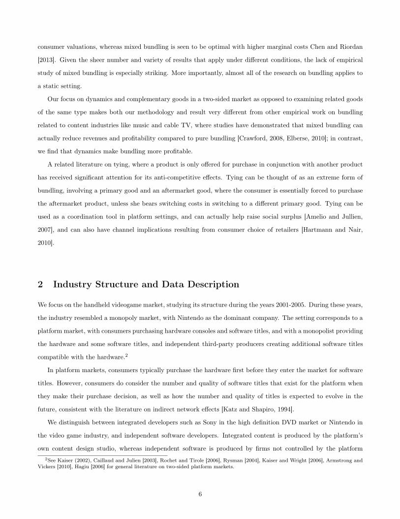
The Dynamic Effects of Bundling as a Product Strategy (Article begins on next page) The Harvard community has made this article openly available. Please share how this access benefits you. Your story matters. Citation Derdenger, Timothy, and Vineet Kumar. "The Dynamic Effects of Bundling as a Product Strategy." Marketing Science (forthcoming). Accessed May 25, 2018 11:15:03 PM EDT Citable Link http://nrs.harvard.edu/urn-3:HUL.InstRepos:11148069 Terms of Use This article was downloaded from Harvard University's DASH repository, and is made available under the terms and conditions applicable to Open Access Policy Articles, as set forth at http://nrs.harvard.edu/urn-3:HUL.InstRepos:dash.current.terms-of- use#OAP
-
Upload
nguyenkien -
Category
Documents
-
view
239 -
download
2
Transcript of The Dynamic Effects of Bundling as a Product Strategy Dynamic Effects of Bundling as a Product...

The Dynamic Effects of Bundling as a Product Strategy
(Article begins on next page)
The Harvard community has made this article openly available.Please share how this access benefits you. Your story matters.
Citation Derdenger, Timothy, and Vineet Kumar. "The Dynamic Effects ofBundling as a Product Strategy." Marketing Science (forthcoming).
Accessed May 25, 2018 11:15:03 PM EDT
Citable Link http://nrs.harvard.edu/urn-3:HUL.InstRepos:11148069
Terms of Use This article was downloaded from Harvard University's DASHrepository, and is made available under the terms and conditionsapplicable to Open Access Policy Articles, as set forth athttp://nrs.harvard.edu/urn-3:HUL.InstRepos:dash.current.terms-of-use#OAP

The Dynamic Effects of Bundling as a Product Strategy
Timothy Derdenger & Vineet Kumar
⇤
Abstract
Several key questions in bundling have not been empirically examined: Is mixed bundling more effective
than pure bundling or pure components? Does correlation in consumer valuations make bundling more or less
effective? Does bundling serve as a complement or substitute to network effects? To address these questions,
we develop a consumer-choice model from micro-foundations to capture the essentials of our setting, the hand-
held video game market. We provide a framework to understand the dynamic, long-term impacts of bundling
on demand. The primary explanation for the profitability of bundling relies on homogenization of consumer
valuations for the bundle, allowing the firm to extract more surplus. We find bundling can be effective through
a novel and previously unexamined mechanism of dynamic consumer segmentation, which operates independent
of the homogenization effect, and can in fact be stronger when the homogenization effect is weaker. We also
find that bundles are treated as separate products (distinct from component products) by consumers. Sales of
both hardware and software components decrease in the absence of bundling, and consumers who had previ-
ously purchased bundles might delay purchases, resulting in lower revenues. We also find that mixed bundling
dominates pure bundling and pure components in terms of both hardware and software revenues. Investigating
the link between bundling and indirect network effects, we find that they act as substitute strategies, with a
lower relative effectiveness for bundling when network effects are stronger.
⇤Both authors contributed equally to this paper, and are listed in alphabetical order.Tim Derdenger is Assistant Professor in Marketing & Strategy, Tepper School of Business, Carnegie Mellon University.e-mail:[email protected] Kumar is Assistant Professor of Business Administration, Marketing Unit, Harvard Business School, Harvard University.e-mail:[email protected] authors would like to thank Sunil Gupta, Brett Gordon and Minjung Park and for comments on an earlier draft of the paper.They gratefully acknowledge feedback from seminar participants at Yale University, Catholic University of Leuven, and the Universityof Zurich as well as conference participants at Marketing Science, Northeastern Marketing Conference and the UT Dallas FORMSconference. All errors remain their own.
1

1 Introduction
Bundling, the practice of including two or more products within a separate product bundle, is arguably the most
flexible element of product strategy, since the component products are already available. Bundling is commonly
used in a diverse range of industries, with examples including fast food (value meals at McDonalds), insurance
(automobile, home and umbrella), telecommunications (home internet & phone service). Bundling is especially
common in technology and content industries, ranging from music albums (bundle of songs), newspapers (bundle
of articles) to cable television (bundle of channels). Bundling could involve both similar products (e.g. season
tickets), and dissimilar or complementary products (e.g. consoles and video games).
It is interesting to note that record companies make both singles and entire albums available for purchase,
whereas most newspapers or online news sites commonly do not allow purchase of individual articles. We thus
find two types of bundling commonly used in practice: pure bundling refers to the practice of selling two or more
discrete products only as part of a bundle, whereas mixed bundling refers to the practice of selling a bundle of
the products as well as the individual products themselves.1 Another example of this dichotomy occurs in office
productivity suites: Microsoft only sells Microsoft Word as part of Microsoft Office (pure bundling), whereas Apple
has moved away from marketing the corresponding Pages software as part of the iWork bundle, and it is currently
available as a pure product. In the smartphone market, both Apple and Google bundle software applications like
Maps and GPS with the hardware and operating system as a pure bundle. The variety of bundling possibilities
in each market and its ease of implementation make bundling an important product strategy decision that hold
significant potential for the firm.
Our objective is to empirically examine the effectiveness of bundling as a product strategy, especially to un-
derstand the dynamic effects of bundling in markets with complementary products, where consumers could derive
additional utility from having both products, e.g. hardware and software, as opposed to having just one or the
other [Nalebuff, 2004]. We seek to understand and answer the following research questions:
1. Cannibalization and Market Expansion: Does bundling result in cannibalization of pure component
products or does it increase overall sales of both products?
2. Bundling Types: Are bundles equivalent to the product components purchased together? Is mixed bundling
(both bundle and component products are available) more effective than pure components or pure bundling?
3. Complementarity and Network Effects: Does the presence and strength of network effects or comple-
mentarity make bundling relatively more or less effective?
1Note that pure components refers to the strategy of selling individual products without bundling.
2

We develop a model to study these dynamics in the setting of handheld video game consoles (hardware) and games
(software), where consumers purchase products of a durable nature, with intertemporal tradeoffs playing a key role
in decision making.
Much prior research has focused on how bundling results in the homogenization of consumer valuations [Adams
and Yellen, 1976, Schmalensee, 1984, McAfee et al., 1989]. The central idea is that a monopolist can use bundles
profitably when consumer valuation for bundles is more homogeneous than for the component products, since this
would enable better extraction of consumer surplus. In the limit, it is easy to see that a monopolist facing a market
of identical consumers can use uniform pricing to achieve complete extraction of consumer surplus.
Our primary contributions are in investigating and helping understand the dynamics of bundling from an
empirical perspective. First, we uncover an additional indepedent mechanism for bundling in dynamic settings,
based on the notion of the bundle serving as a product to achieve more effective dynamic consumer segmentation.
The presence of bundles causes some consumers to advance their purchases from later periods to earlier periods,
resulting in more effective consumer segmentation over time. Broadly, we find that bundling can be effective under
a much wider range of conditions in a dynamic setting than proposed by the literature. Our findings provide more
insight into an alternative mechanism that can make bundling especially effective in markets with intertemporal
tradeoffs and significant consumer heterogeneity, e.g. durable goods like automobiles, consumer electronics and in
technology markets where tradeoffs on when to purchase as especially important. Second, we find that bundles
serve a role similar to an additional product in the firm’s product offering, since consumers do not value the bundle
identical to the sum of valuations of the component products. We also find that the presence of bundles increases the
sales of both component products, thus magnifying its beneficial effects. Third, we empirically examine the nature
and effectivenenss of different approaches to bundling, i.e. mixed bundling versus pure bundling ; the theoretical
literature has found support for either choice to be dominant depending on the setting and conditions [Chen and
Riordan, 2013, McAfee et al., 1989]. We find that relative to pure components, mixed bundling enhances revenues
for both hardware and software, whereas pure bundling diminishes sales of both types of products. Finally, we
examine the interaction between bundling and network effects, and find that they serve as substitutes, i.e. bundling
is more effective in settings with weaker network effects, suggesting that managers might find it useful to bundle
in settings where the network effect is weaker.
Since prior research on bundling has been mostly been developed for static settings, the dynamic segmentation
mechanism is a novel discovery. Indeed, it is easy to see why this mechanism is more effective when consumer
valuations for the two product components is positively correlated, i.e. consumers have high valuations for both
hardware and software, or low valuations for both. In such a market, we find that consumers with low valuation for
hardware and software intertemporally substitute and accelerate their hardware purchases when bundles discounted
from sum of component prices are available as an option. As expected, we find that heterogeneity plays a crucial
3

role in how bundling becomes effective, with more heterogenity increasing the effectiveness of bundling. The
company’s revenues for hardware are increased with bundling, and the intertemporal substitution effect of low
valuation consumers plays a significant role. Thus, we find that bundling increases revenues because consumers
with low hardware valuations accelerate their purchases in the presence of bundles, but high valuation consumers
still find individual consoles to provide flexibility in making software purchases, and of high enough value not to
substitute away from a choice of pure console.
From a methodological perspective, we provide a new strategy to identify correlation between consumer prefer-
ences for complementary products, i.e. hardware and software, using aggregate data. Our identification argument
is based on how the tying ratio (ratio of software sales to hardware installed base) varies dynamically and does
not rely on the presence of bundles. We also incorporate an explicit microfoundations-based link between the
hardware market and software that could be purchased by modeling consumer preferences across the set of possible
portfolios that the consumer could potentially purchase over time; such an explicit model of expectation of possible
consumer holdings in a market (software) has not been incorporated in another market (hardware) to the best of
our knowledge. Consumers place a higher value on hardware when there are more and better games available at
lower prices in the software market, and when more games are expected to become available in future periods.
Most other research in the marketing literature model the indirect network effect with a reduced form approach,
often using the number of products available as proxy, e.g. [Dube et al., 2010], while focusing on other dimensions
of the model.
Our model incorporates the durable nature of products, so that consumers choose between purchasing versus
waiting. The timing of the model is as follows: consumers who do not own hardware must decide whether or not
to purchase a console or bundle each period until they make a purchase. When consumers purchase a console
or bundle, they exit the hardware market and enter the software market. In each period in the software market,
consumers make decisions regarding whether and which game to purchase, depending on the available choice set
for games.
The framework uses the approach of tractably characterizing an inclusive value, and builds upon dynamic
demand frameworks Melnikov [2013], Hendel and Nevo [2006], Gowrisankaran and Rysman [2012], which in turn
are based on the BLP model [Berry et al., 1995], and we extend this framework along a number of dimensions. We
approximate the expected future value of both consoles and games separately as the inclusive value for hardware
and for software. The inclusive value is the present discounted value of making a purchase in the current period,
and consumers form expectations over the evolution of the inclusive value. The inclusive value abstraction is
designed to tractably capture the possible variations in product availability, pricing and other unobservable factors
that might evolve over time, collapsing multiple dimensions of the state space to two dimensions, one each for
the hardware and software markets. Similar to other dynamic demand models, we also abstract away supply-side
4

decisions like product development and design, although we do evaluate different supply-side configurations for
bundling as counterfactuals.
Although we use the setting of handheld video game consoles and games, the mechanisms we propose are
more general and could be found in other dynamic settings. Our findings point to practically relevant and highly
significant results for product strategy and management. Since bundles are created rather easily in most contexts,
we expect this to be a practical and easily achievable option for firms across a variety of industries.
Related Literature
The phenomenon of bundling, both of the pure and mixed varieties has received much attention in the theoretical
literature in marketing and economics. However, there has been little empirical understanding of the effects of
bundling, which is clearly required to characterize both the short-term product substitution effects as well as
dynamic long-term demand enhancing effects we seek to study.
A survey of the major practical tradeoffs in constructing bundles at a conceptual and theoretical level is presented
in Venkatesh et al. [2009]. Tellis and Stremersch [2002] present a detailed characterization of the types of bundling
and their optimality under different conditions, and distinguish between product bundling and price bundling.
Bundling has traditionally been considered a price discrimination strategy to extract more surplus from consumers
who have heterogeneous valuations for different products, as illustrated in early work by Adams and Yellen [1976],
and modeled in further detail [Schmalensee, 1984, McAfee et al., 1989]. These papers recognize that consumer
heterogeneity is the primary reason why a monopolist would not be able to extract full surplus from consumers,
and contribute the key idea that heterogeneity in valuation across consumers can be diminished by bundling
multiple products. Recall that consumer heterogeneity is a primary reason that a monopolist cannot fully extract
all surplus from consumers. The reduction in heterogeneity due to bundling happens because the variance in the
sum of product valuations is lower than the sum of variances in product valuations, which then allows a monopolist
to more effectively extract surplus. Bakos and Brynjolfsson [1999] have examined bundling for information goods
and considered the presence of a menu of bundles on consumer choices with large bundles using asymptotic theory,
whereas Fang and Norman [2006] provide exact results for the general case of a monopolist bundling a finite number
of goods.
Recent research on mixed bundling indicates that this strategy is likely to be more profitable when the products
to be bundled are sufficiently asymmetric in production costs as well as network effects [Prasad et al., 2010], whereas
more similarity between products makes pure bundling or pure components profitable. It is noteworthy that the
authors point to the lack of empirical research at the confluence of network effects and bundling, echoing more
general calls for an empirical measurement of the market effects of bundling [Kobayashi, 2005]. With regard to
the specific types of bundling, there is evidence for pure bundling dominating under low marginal costs relative to
5
consumer valuations, whereas mixed bundling is seen to be optimal with higher marginal costs Chen and Riordan
[2013]. Given the sheer number and variety of results that apply under different conditions, the lack of empirical
study of mixed bundling is especially striking. More importantly, almost all of the research on bundling applies to
a static setting.
Our focus on dynamics and complementary goods in a two-sided market as opposed to examining related goods
of the same type makes both our methodology and result very different from other empirical work on bundling
related to content industries like music and cable TV, where studies have demonstrated that mixed bundling can
actually reduce revenues and profitability compared to pure bundling [Crawford, 2008, Elberse, 2010]; in contrast,
we find that dynamics make bundling more profitable.
A related literature on tying, where a product is only offered for purchase in conjunction with another product
has received significant attention for its anti-competitive effects. Tying can be thought of as an extreme form of
bundling, involving a primary good and an aftermarket good, where the consumer is essentially forced to purchase
the aftermarket product, unless she bears switching costs in switching to a different primary good. Tying can be
used as a coordination tool in platform settings, and can actually help raise social surplus [Amelio and Jullien,
2007], and can also have channel implications resulting from consumer choice of retailers [Hartmann and Nair,
2010].
2 Industry Structure and Data Description
We focus on the handheld videogame market, studying its structure during the years 2001-2005. During these years,
the industry resembled a monopoly market, with Nintendo as the dominant company. The setting corresponds to a
platform market, with consumers purchasing hardware consoles and software titles, and with a monopolist providing
the hardware and some software titles, and independent third-party producers creating additional software titles
compatible with the hardware.2
In platform markets, consumers typically purchase the hardware first before they enter the market for software
titles. However, consumers do consider the number and quality of software titles that exist for the platform when
they make their purchase decision, as well as how the number and quality of titles is expected to evolve in the
future, consistent with the literature on indirect network effects [Katz and Shapiro, 1994].
We distinguish between integrated developers such as Sony in the high definition DVD market or Nintendo in
the video game industry, and independent software developers. Integrated content is produced by the platform’s
own content design studio, whereas independent software is produced by firms not controlled by the platform2See Kaiser (2002), Caillaud and Julien [2003], Rochet and Tirole [2006], Rysman [2004], Kaiser and Wright [2006], Armstrong and
Vickers [2010], Hagiu [2006] for general literature on two-sided platform markets.
6

manufacturer. In addition to selling access to consumers and producing content, the platform can also offer a
bundle of the hardware and software developed by its integrated development studio, as is the case in our setting.
Both hardware and software, including consoles, games and bundles were primarily marketed and sold through
brick-and-mortar retailers in the time period corresponding to our data. The bundles were packaged by the
manufacturer (Nintendo), and only included select games from their own integrated studio.
Data
The data used in this study originates from the marketing group NPD; they track sales and pricing for the
video game industry and collect data using point-of-sale scanners linked to a majority of the consumer electronics
retail stores in the United States. NPD extrapolates the data to project sales for the entire country. Included in
the data are quantity sold and total revenue for two consoles and three bundles and all of their compatible video
games, numbering approximately 700.
The data set covers 45 months starting in June 2001 and continues through February 2005, during which time
Nintendo was a monopolist in the portable video game market, and before Sony’s PlayStation Portable entered the
market. Nintendo was a multi-product monopolist producing two versions of its very popular Game Boy Advance
(GBA) console as well as a portfolio of games to be played on its console. Each version was internally identical, but
the second version dubbed the GBA SP was reoriented with the display placed horizontally rather than vertically.
The GBA SP looked like a mini laptop computer and was close to half the size of the original GBA. Moreover,
it is usually the case with the introduction of a new device that new games are released which are not backwards
compatible. However, with the introduction of the GBA SP, the internal hardware of both devices were essentially
identical, and both devices could share the same set of games.
The target market of these two devices was younger kids rather than teenagers or young adults, which were
the targeted demographic segments for the home video game console. Portable or handheld consoles differ from
traditional home video game consoles, since they are mobile, with the size of the device being no larger than an
adult hand. The devices are designed to easily travel with a consumer and can be played in a car or airplane,
whereas a home console is restricted to locations with a television display and electricity.
General statistics of the portable video game industry are provided in the tables below. We also present a plot
of aggregate sales data for hardware and software in Figure 2.3 In Tables 1 and 2, we present statistics on the
release date, total units sold and the number of months on the console market, average (min and max) prices and
total units sold for each of the two standalone consoles and three bundles.3 Sales data is presented in its raw and deseasoned form, where the data is deseasoned with the use of the X11 program from the
US Census.
7
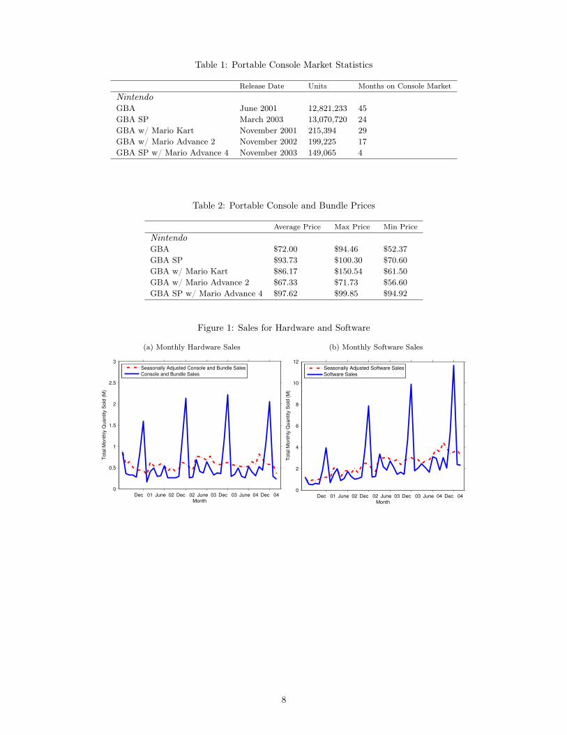
Table 1: Portable Console Market Statistics
Release Date Units Months on Console MarketNintendoGBA June 2001 12,821,233 45
GBA SP March 2003 13,070,720 24
GBA w/ Mario Kart November 2001 215,394 29
GBA w/ Mario Advance 2 November 2002 199,225 17
GBA SP w/ Mario Advance 4 November 2003 149,065 4
Table 2: Portable Console and Bundle Prices
Average Price Max Price Min PriceNintendoGBA $72.00 $94.46 $52.37
GBA SP $93.73 $100.30 $70.60
GBA w/ Mario Kart $86.17 $150.54 $61.50
GBA w/ Mario Advance 2 $67.33 $71.73 $56.60
GBA SP w/ Mario Advance 4 $97.62 $99.85 $94.92
Figure 1: Sales for Hardware and Software
(a) Monthly Hardware Sales
Dec 01 June 02 Dec 02 June 03 Dec 03 June 04 Dec 040
0.5
1
1.5
2
2.5
3
Tota
l Month
ly Q
uantit
y S
old
(M
)
Month
Seasonally Adjusted Console and Bundle SalesConsole and Bundle Sales
(b) Monthly Software Sales
Dec 01 June 02 Dec 02 June 03 Dec 03 June 04 Dec 040
2
4
6
8
10
12
Tota
l Month
ly Q
uantit
y S
old
(M
)
Month
Seasonally Adjusted Software SalesSoftware Sales
8
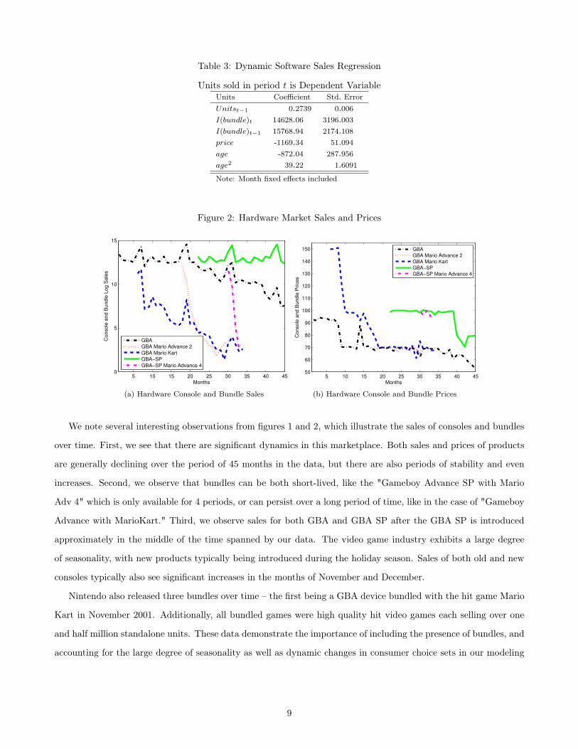
Table 3: Dynamic Software Sales Regression
Units sold in period t is Dependent VariableUnits Coefficient Std. ErrorUnitst�1 0.2739 0.006I(bundle)t 14628.06 3196.003I(bundle)t�1 15768.94 2174.108price -1169.34 51.094age -872.04 287.956age
2 39.22 1.6091
Note: Month fixed effects included
Figure 2: Hardware Market Sales and Prices
5 10 15 20 25 30 35 40 450
5
10
15
Months
Co
nso
le a
nd
Bu
nd
le L
og
Sa
les
GBAGBA Mario Advance 2GBA Mario KartGBA!SPGBA!SP Mario Advance 4
(a) Hardware Console and Bundle Sales
5 10 15 20 25 30 35 40 4550
60
70
80
90
100
110
120
130
140
150
Months
Console
and B
undle
Prices
GBA
GBA Mario Advance 2
GBA Mario Kart
GBA!SP
GBA!SP Mario Advance 4
(b) Hardware Console and Bundle Prices
We note several interesting observations from figures 1 and 2, which illustrate the sales of consoles and bundles
over time. First, we see that there are significant dynamics in this marketplace. Both sales and prices of products
are generally declining over the period of 45 months in the data, but there are also periods of stability and even
increases. Second, we observe that bundles can be both short-lived, like the "Gameboy Advance SP with Mario
Adv 4" which is only available for 4 periods, or can persist over a long period of time, like in the case of "Gameboy
Advance with MarioKart." Third, we observe sales for both GBA and GBA SP after the GBA SP is introduced
approximately in the middle of the time spanned by our data. The video game industry exhibits a large degree
of seasonality, with new products typically being introduced during the holiday season. Sales of both old and new
consoles typically also see significant increases in the months of November and December.
Nintendo also released three bundles over time – the first being a GBA device bundled with the hit game Mario
Kart in November 2001. Additionally, all bundled games were high quality hit video games each selling over one
and half million standalone units. These data demonstrate the importance of including the presence of bundles, and
accounting for the large degree of seasonality as well as dynamic changes in consumer choice sets in our modeling
9

framework.
To get an approximate idea of the dynamics of video game software sales (in units), we regress the current period
sales as a function of lagged sales, current price, age and age2 as well as an indicator for whether there is a bundle
present in the current or previous period:
s
g,t
= ✓1 sg,t�1 + ✓2I(bundlet) + ✓3I(bundlet�1) + ✓4 pg,t + ✓5 age+ ✓6 age2+ !
g,t
(1)
where !g,t
is distributed iid as a standard normal random variable. We estimate the above specification using
the Arellano-Bond GMM estimation procedure given the endogeneity of the one period lagged measure of the
dependent variable and price using standard instruments of lagged regessors.
Examining the results of the regression in Table 3, we find that having a bundle sold in period t or t � 1 is
associated with increased software sales, age appears to have a negative effect on sales, while the positive coefficient
on age
2 indicates that the magnitude of the marginal effect is diminished as the game ages. This finding implies
that there is likely to be pent up demand for games, and significant sales are achieved quickly after product release,
beyond which sales decline. Note that the above analysis is not intended to serve as a causal account, given the
multiple concerns it might raise, including endogeneity. Rather we use these results along with the model-free
evidence in Figure 1 to motivate the need for investigating the dynamics of the market by modeling the micro-
foundations of consumer decisions, which help in explaining and understanding these dynamic data patterns.
3 Model
We develop a model that captures the essentials of our institutional setting and consumer buying behavior,
and is suitable for use with aggregate market data. Consider the consumer decision journey, which begins in the
hardware market. When a consumer is present in the hardware market, she makes a discrete choice from the set
of available consoles or bundles or decides not to make a purchase. After purchasing a hardware unit, she exits the
hardware market and enters the software market, where she may purchase a video game in each period, or make
no purchase. The timeline of the consumer journey is detailed in Figure 3.
There are several specific details of our institutional setting that must be captured by our model to ensure that
the effects of bundling are appropriately characterized:
• Dynamics: There are several sources of dynamics in the model, including firm driven variations such as price
changes, variation in product availability for consoles, video games and bundles, as well as consumer dynamics
due to entry and exit of consumers from the hardware and software markets. In durable goods settings such
as ours, consumers face the option of delaying buying, and their purchases continue to provide flow utility in
future periods following purchase. Another issue that contributes to dynamics in our setting is the inherent
seasonality in purchases of videogame consoles and games, which we aim to explicitly incorporate.
10
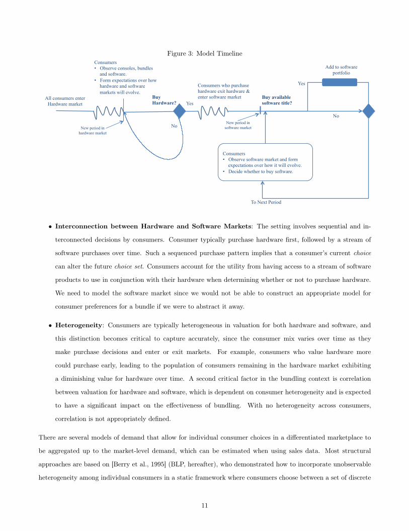
Figure 3: Model Timeline
All consumers enter Hardware market
Consumers • Observe consoles, bundles
and software. • Form expectations over how
hardware and software markets will evolve.
Yes
No
Buy Hardware?
Consumers • Observe software market and form
expectations over how it will evolve. • Decide whether to buy software.
New period in hardware market
To Next Period
No New period in
software market
Buy available software title?
Yes
Add to software portfolio
Consumers who purchase hardware exit hardware & enter software market
• Interconnection between Hardware and Software Markets: The setting involves sequential and in-
terconnected decisions by consumers. Consumer typically purchase hardware first, followed by a stream of
software purchases over time. Such a sequenced purchase pattern implies that a consumer’s current choice
can alter the future choice set. Consumers account for the utility from having access to a stream of software
products to use in conjunction with their hardware when determining whether or not to purchase hardware.
We need to model the software market since we would not be able to construct an appropriate model for
consumer preferences for a bundle if we were to abstract it away.
• Heterogeneity: Consumers are typically heterogeneous in valuation for both hardware and software, and
this distinction becomes critical to capture accurately, since the consumer mix varies over time as they
make purchase decisions and enter or exit markets. For example, consumers who value hardware more
could purchase early, leading to the population of consumers remaining in the hardware market exhibiting
a diminishing value for hardware over time. A second critical factor in the bundling context is correlation
between valuation for hardware and software, which is dependent on consumer heterogeneity and is expected
to have a significant impact on the effectiveness of bundling. With no heterogeneity across consumers,
correlation is not appropriately defined.
There are several models of demand that allow for individual consumer choices in a differentiated marketplace to
be aggregated up to the market-level demand, which can be estimated when using sales data. Most structural
approaches are based on [Berry et al., 1995] (BLP, hereafter), who demonstrated how to incorporate unobservable
heterogeneity among individual consumers in a static framework where consumers choose between a set of discrete
11

alternatives.
The BLP framework has been extended to incorporate dynamic effects with forward-looking consumers [Mel-
nikov, 2013, Hendel and Nevo, 2006, Gowrisankaran and Rysman, 2012, Schiraldi, 2011]. We base our model on the
inclusive value approach suggested by Melnikov [2013] and further expanded by Gowrisankaran and Rysman [2012]
(G&R, hereafter), who formulate a model of dynamic demand where the evolution of the market is captured by a
single inclusive value variable representing dynamic purchase utility that is specific to an individual consumer and
varies over time. This specification has an intuitive interpretation and captures the dynamics in a parsimonious
manner, enabling the development of a tractable model that aggregates the behavior of forward-looking consumers,
and allows for estimation with market-level data. The idea of collapsing the entire state space into an inclusive
variable allows us to capture multiple sources of dynamics in a tractable manner. Such dynamic changes might
include a rich array of possibly uncertain dimensions, e.g. the introduction of new hardware and software prod-
ucts and their features, price changes, promotions that are unobservable to the researcher. An alternative way
to approach this problem is to choose a small number of primary dimensions of interest, and model a consumer
expectation process for those specific variables, e.g. Gordon [2009], in his study of the personal computer market
considers the CPU Speed as the primary quality dimension, and the price as an additional dimension which helps
keep the state space tractable.
There are multiple approaches to modeling the interconnection between hardware and software markets. One
approach is to just include the number of games like [Nair et al., 2004, Dube et al., 2010], but in our case we would
not be able to capture the bundle’s included software appropriately. Another would be to model the software
utility like Gowrisankaran et al. [2010], who account for a consumer’s portfolio of owned products explicitly but
link consumer preference structures across hardware and software markets only by using the number of available
products. A third would be to abstract the model so that software titles are independent, allowing the expectation
of the software utility to be integrated in the hardware market like in Lee [2013], where consumers in the hardware
market explicitly account for the utility obtained by future software purchases in their hardware decision-making.
We believe the present paper is the first to model the software portfolio explicitly and incorporate the utility from
a portfolio of (software) content into the utility of purchasing in another (hardware) market, and we would expect
modeling the portfolio to be important since the number of software titles owned may have diminishing marginal
utility, which would not be captured without including consumer holdings, thus biasing the results.
To aid in exposition, we begin our description of the consumer utility in reverse sequential order, beginning with
software purchase decisions made by consumers. We must emphasize that, like in other durable goods settings,
consumers examine the dynamic stream of utilities obtained from a purchase when they make the decision to
purchase or not purchase, and the utilities in §3.1 and §3.2 below are not sufficient for consumer decision-making,
which is detailed in § 3.3.
12
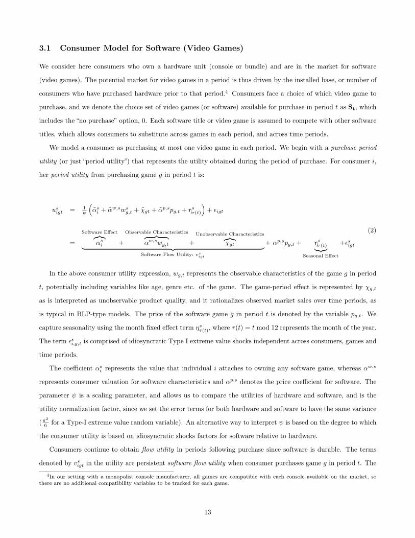
3.1 Consumer Model for Software (Video Games)
We consider here consumers who own a hardware unit (console or bundle) and are in the market for software
(video games). The potential market for video games in a period is thus driven by the installed base, or number of
consumers who have purchased hardware prior to that period.4 Consumers face a choice of which video game to
purchase, and we denote the choice set of video games (or software) available for purchase in period t as St, which
includes the “no purchase” option, 0. Each software title or video game is assumed to compete with other software
titles, which allows consumers to substitute across games in each period, and across time periods.
We model a consumer as purchasing at most one video game in each period. We begin with a purchase period
utility (or just “period utility”) that represents the utility obtained during the period of purchase. For consumer i,
her period utility from purchasing game g in period t is:
u
s
igt
=
1
⇣
↵
s
i
+ ↵
w,s
w
s
g,t
+ �
gt
+ ↵
p,s
p
g,t
+ hs⌧(t)
⌘
+ ✏
igt
=
Software Effectz}|{
↵
s
i
+
Observable Characteristicsz }| {
↵
w,s
w
g,t
+
Unobservable Characteristicsz}|{
�
gt
| {z }
Software Flow Utility: v
s
igt
+ ↵
p,s
p
g,t
+ hs⌧(t)|{z}
Seasonal Effect
+✏
s
igt
(2)
In the above consumer utility expression, wg,t
represents the observable characteristics of the game g in period
t, potentially including variables like age, genre etc. of the game. The game-period effect is represented by �
g,t
as is interpreted as unobservable product quality, and it rationalizes observed market sales over time periods, as
is typical in BLP-type models. The price of the software game g in period t is denoted by the variable p
g,t
. We
capture seasonality using the month fixed effect term ⌘
s
⌧(t), where ⌧(t) = t mod 12 represents the month of the year.
The term ✏
s
i,g,t
is comprised of idiosyncratic Type I extreme value shocks independent across consumers, games and
time periods.
The coefficient ↵s
i
represents the value that individual i attaches to owning any software game, whereas ↵w,s
represents consumer valuation for software characteristics and ↵
p,s denotes the price coefficient for software. The
parameter is a scaling parameter, and allows us to compare the utilities of hardware and software, and is the
utility normalization factor, since we set the error terms for both hardware and software to have the same variance
(⇡2
6 for a Type-I extreme value random variable). An alternative way to interpret is based on the degree to which
the consumer utility is based on idiosyncratic shocks factors for software relative to hardware.
Consumers continue to obtain flow utility in periods following purchase since software is durable. The terms
denoted by v
s
igt
in the utility are persistent software flow utility when consumer purchases game g in period t. The
4In our setting with a monopolist console manufacturer, all games are compatible with each console available on the market, sothere are no additional compatibility variables to be tracked for each game.
13

flow utility is persistent across time periods, whereas the other terms in the period utility are only obtained during
the period when the consumer makes a purchase. Consumer i thus receives period utility u
s
igt
in the period of
purchase t, and continues to receive flow utility�
v
s
igt
�
in all periods ! > t after purchasing, where the flow utility
is fixed during the period of purchase.
Since consumers are forward looking and the product is a durable good, consumers do not make the decision to
purchase based only on the above period utility or flow utility – these serve as “building blocks” for the consumer
decision making process, detailed in §3.3. The consumer has expectations about the choices she might make in the
future and how her current choice would impact the future, she would continue obtaining flow utility in periods
following a purchase.
3.2 Consumer Model for Hardware (Consoles and Bundles)
We develop a model of hardware choice, where consumers indexed by set I consider whether or not to purchase
hardware from the set of available consoles Jt or bundles Bt. The overall choice set for a consumer in the hardware
market is then Ht = {0} [ Jt[Bt. We model only consumers who have not purchased a console or a bundle to make
up the hardware market of potential buyers for bundles. Although consumers consider the entire set of hardware
available when making a purchase decision, for simplicity of exposition we first outline the utility specification for
consoles, followed by bundles. Consumers who make a hardware purchase exit the hardware market permanently.
Note that choice sets are allowed to vary over time.
Consoles
Consider the decision process when only consoles are available in the market: in each period, consumers can choose
to purchase a console, provided they have not already purchased a console in the past.5 Consumer i 2 I determines
in period t 2 T whether or not to purchase console j 2 Jt, and we denote this decision as dijt
2 {0, 1}. Consoles are
durable and consumers receive a stream of flow utilities in all periods following a purchase. If consumer i decides
to purchase console j in period t (dijt
= 1), he will obtain a purchase period utility given by:6
u
c
ijt
=
Hardware Effectz}|{
↵
h
i
+
Observable Characteristicsz }| {
↵
x,h
x
j,t
+
Unobservable Characteristicsz}|{
⇠
jt
| {z }
Console Flow Utility: v
h
ijt
+
Indirect Network Effectz }| {
W
c
it
(3)
+ ↵
p,h
p
j,t
+ ⌘
h
⌧(t)|{z}
Seasonal Effect
+✏
c
i,j,t
(4)
5For households with multiple users that purchase multiple consoles, our model would treat them as separate consumers, in linewith the current literature on aggregate demand models.
6Similar to the software market, the consumer does not make the decision to purchase based only on the period utility. Thedecision-making process is detailed in §3.3.
14

Each console is characterized by both observable product characteristics x
j,t
and an unobservable product charac-
teristic ⇠jt
, which may vary both over time as well as across consoles. Note that the unobserved characteristic ⇠jt
is observed by consumers and accounted for by the console manufacturer, but is not observed by the researcher.
Consistent with BLP, this characteristic could include product characteristics like style and design and usability as
well as all other factors that are not present in the data.
The period utility of a console is also directly related to the games available for the consumer to purchase, and
should incorporate the consumer’s expectation of how the software market might evolve after purchasing hardware.
We thus include the utility from software into the consumer’s hardware utility function, using the term W
c
it
to
represent the present discounted scaled software utility available for the platform in period t and the consumer’s
expectation of how it may evolve in the future. The issue is whether the expected value of software purchases is
obtained as a flow utility after the consumer has purchased hardware and entered the software market. Consider
two alternative viewpoints on this matter. First, if we interpret W
c
it
as the option value of being present on the
software market, then we would expect the consumer to obtain it as part of the flow utility. On the other hand,
if it’s interpreted as purely the expected discounted flow of utilities from optimal future purchases made in the
software market, then it would make sense for the term to be excluded from the flow utility of hardware. We choose
the latter interpretation and exclude the indirect network effect from the flow utility, although it does enter the
purchase period utility.
Note that unike most empirical research modeling two-sided markets in Marketing, we structurally connect the
hardware and software markets which both involve dynamic demand with forward-looking consumers, explicitly
incorporating the utility of purchasing software into the hardware utility term. We detail explicitly the specific
form of this connection between the markets in § 3.4 below.
The price of console j in period t is denoted p
j,t
. We capture seasonality in the hardware market with the
month fixed effect term ⌘
h
⌧(t) where ⌧(t) = t mod 12 represents the month of the year. The idiosyncratic shock
specific to the consumer, console and period ✏cijt
is unobservable and independently distributedas a Type I extreme
value random variable, and is uncorrelated with all other unobservables in the model.
The coefficient ↵h
i
denotes the degree to which consumer i values a console, whereas ↵x,h indicates the effect of
consoles characteristics on the consumer’s utility and finally ↵p,h is the consumer’s price coefficient. Note that the
terms denoted by v
h
ijt
in the utility are deterministic persistent flow utility in the event of a purchase in period t.
If consumer i purchases the product j in period t, then she exits the hardware market, and continues to receives a
flow-utility in each period ⌧ > t equal to v
h
ijt
, which is fixed at the time of purchase.
15

Bundles
The above utility specification for hardware only considered consoles; however, in addition to consoles, consumers
also have the choice to purchase a bundle of a console and a video game in periods when a bundle is available.
We denote this selection by Bt, where a bundle b 2 Bt is represented as b = (j, g), i.e. the bundle comprises
of hardware console j and software game g. In periods where there is no bundle available in the market, we set
Bt = ; and consumers in those periods can only purchase consoles and games, i.e. pure components. Note that if
the consumer purchases a bundle b = (j, g), she exits the market for hardware (bundles and consoles).
When consumer i considers the bundle option, the purchase period utility she derives from the purchase of
bundle b = (j, g) in period t is given by u
b
ibt
:
u
b
ibt
=
Total Bundle Flow: v
b
ibt
z }| {
↵
h
i
+ ↵
x,h
x
jt
| {z }
Hardware Flow: v
h
ijt
�⇠jt
+ ↵
s
i
+ ↵
w,s
w
gt
| {z }
Software Flow: v
s
igt
��gt
+µ
bt
+ ↵
b
|{z}
Bundle Effect
+ W
b
it
+ ↵
p,h
p
b,t
+ ⌘
b
⌧(t)|{z}
Seasonal Effects
+ ✏
b
ibt
(5)
Thus, for consumer i, the utility of a bundle b = (j, g) includes the deterministic components of the utility of console
j, i.e. v
h
ijt
and the utility of the game that is included, vsigt
. Note that the unobservable terms from the console
j and video game g corresponding to the bundle, ⇠j,t
and �
g,t
do not appear in the bundle utility function since
they are product-specific unobservables and the bundle is positioned as a distinct product. Therefore, a BLP-type
bundle-specific unobservable characteristic µ
bt
is included in the persistent flow utility, and would include design,
usability and other factors that may impact its utility above and beyond the utility of its constituent console and
video game. Such a formulation recognizes that bundles are separate products in their own right. We capture a
generic effect of purchasing a bundle using ↵b as the additional value that consumers have for the bundle over and
beyond the value of the constituent hardware console and software game.
The idiosyncratic shock specific to the consumer, bundle and period, ✏bibt
is again assumed to be distributed iid
as Type I extreme value and uncorrelated with the other unobservables. We assume that µ
bt
does persist beyond
the period in which it is purchased, i.e. it appears in the flow utility of the bundle, and the terms denoted by v
b
ibt
in the utility are persistent “flow utility” in the event of a purchase. Thus, consumer i who has purchased a bundle
b in period t continues to receive a flow-utility of vbibt
in period ⌧ > t, where the flow utility is fixed at the time
of purchase. However, consistent with the model for consoles and for software, the bundle seasonal effect is not
persistent in the model. As in the console model, we define the specific form of connection between the markets,
or the indirect network effect, W b
it
in § 3.4 below.
To complete the hardware model, we assume a consumer i who is on the hardware market and decides not to
purchase any hardware, console or bundle in period t receives utility ✏i,0,t, while retaining the option to purchase
hardware in future periods. Thus, the the vector of hardware error terms for consumer i in period t is ✏Hit =
16

⇣
✏
i0t, ✏c
i,1,t, . . . , ✏c
i,|Jt
|,t, ✏b
i,1,t . . . , ✏b
i,|Bt
|,t
⌘
, which are independently distributed across consumers, products and time
periods.
Lastly, we fix consumers’ price sensitivity to be equal for hardware and software, i.e. ↵
p,s
=
↵
p,h
. From a
structural viewpoint, the price coefficient for consumers might be different for hardware and software only when
the purchase of a hardware console would cause a change in wealth, leading to a change in price-sensitivity.7 We
note that consumer heterogeneity enters through the preference for consoles and gaming in general (a hardware
constant and software constant), and all other coefficients are homogeneous in our model specification.
3.3 Consumer’s Decision Problem
We now describe consumer decisions in chronological order, beginning with the hardware market, followed by those
in the software market.
3.3.1 Hardware Market Decisions
Consumers in the hardware market are forward-looking and in period t purchase a console or bundle after evaluating
dynamic utilities from options available in that period and forming expectations over the evolution of both hardware
and software markets. When a consumer purchases a bundle or console, she exits the hardware market and does
not return to it in future periods, and she enters the software market. Given this setup, the decision problem is
inherently dynamic, and the consumer faces a choice of when to purchase hardware.
Consider consumer i’s decision problem for the console or bundle in a specific period, t: she has to decide
whether to buy a hardware product now or wait until the next period to make a similar decision. In order to
account for the value of waiting, followed by adoption at some point in the future, the consumer has to anticipate
the evolution of all variables ⌦
i,t
that will affect the value of the future adoption decision. The state ⌦
i,t
ideally
ought to include the future evolution of console characteristics (both observable and unobservable), entry of new
hardware, i.e. consoles or bundles, future price trajectory, as well the video games that might be available in the
future software market, since each of these variables might affect the utility of a future hardware adoption.
For consumer i, the Bellman equation that describes her value for being in a current state ⌦
h
i,t
in the hardware
market is given by the recursive relationship:
V
h
i
(f
it
,⌦
h
i,t
, ✏
hit) = max
8
>
>
>
<
>
>
>
:
max
h2Ht\{0}
�
u
iht
(✏
iht
) + �E
⇥
V
i
�
v
h
iht
,⌦
h
i,t+1, ✏hi,t+1
�
�
⌦
h
it
�⇤
| {z }
Purchase hardware h
, � E⇥
V
h
i
�
f
it
,⌦
h
i,t+1, ✏hi,t+1|⌦i,t
�⇤
+ ✏
h
i0t| {z }
No Purchase
9
>
>
>
=
>
>
>
;
(6)7We ought to expect this effect to be very small in our setting, given the low price of consoles, relative to average income levels;
indeed, our results when using different price coefficients for hardware and software are quantitatively very similar and qualitativelythe same as with the primary specification.
17
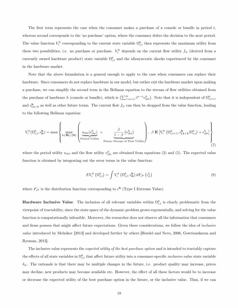
The first term represents the case when the consumer makes a purchase of a console or bundle in period t,
whereas second corresponds to the ‘no purchase’ option, where the consumer defers the decision to the next period.
The value function V
h
i
corresponding to the current state variable ⌦
h
i,t
then represents the maximum utility from
these two possibilities, i.e. no purchase or purchase. V
h
i
depends on the current flow utility f
it
(derived from a
currently owned hardware product) state variable ⌦
h
i,t
and the idiosyncratic shocks experienced by the consumer
in the hardware market.
Note that the above formulation is a general enough to apply to the case when consumers can replace their
hardware. Since consumers do not replace hardware in our model, but rather exit the hardware market upon making
a purchase, we can simplify the second term in the Bellman equation to the stream of flow utilities obtained from
the purchase of hardware h (console or bundle), which is�
P1⌧=t+1 �
⌧�t
v
h
iht
�
. Note that it is independent of ⌦h
i,t+1
and ✏hi,t+1 as well as other future terms. The current flow f
it
can then be dropped from the value function, leading
to the following Bellman equation:
V
h
i
(⌦
h
i,t
, ✏
hit) = max
8
>
>
>
<
>
>
>
:
max
h2Ht\{0}
0
B
B
B
@
u
iht
(✏
h
iht
)
| {z }
Period Utility
+
�
1� �
�
v
h
iht
�
| {z }
Future Stream of Flow Utility
1
C
C
C
A
, � E⇥
V
h
i
�
⌦
h
i,t+1, ✏hi,t+1|⌦
h
i,t
�
+ ✏
h
i0t
⇤
9
>
>
>
=
>
>
>
;
(7)
where the period utility u
iht
and the flow utility v
h
iht
are obtained from equations (3) and (5). The expected value
function is obtained by integrating out the error terms in the value function:
EV
h
i
�
⌦
h
i,t
�
=
ˆV
h
i
�
⌦
h
i,t
, ✏
hit
�
dF
✏
h
�
✏
h
it
�
(8)
where F
✏
h is the distribution function corresponding to ✏h (Type I Extreme Value).
Hardware Inclusive Value The inclusion of all relevant variables within ⌦
h
i,t
is clearly problematic from the
viewpoint of tractability, since the state space of the dynamic problem grows exponentially, and solving for the value
function is computationally infeasible. Moreover, the researcher does not observe all the information that consumers
and firms possess that might affect future expectations. Given these considerations, we follow the idea of inclusive
value introduced by Melnikov [2013] and developed further by others [Hendel and Nevo, 2006, Gowrisankaran and
Rysman, 2012].
The inclusive value represents the expected utility of the best purchase option and is intended to tractably capture
the effects of all state variables in ⌦
h
i,t
that affect future utility into a consumer-specific inclusive-value state variable
�
it
. The rationale is that there may be multiple changes in the future, i.e. product quality may increase, prices
may decline, new products may become available etc. However, the effect of all these factors would be to increase
or decrease the expected utility of the best purchase option in the future, or the inclusive value. Thus, if we can
18

characterize how the inclusive value evolves over time, we can capture all the key drivers of the consumer’s decision
making process. This approach requires the inclusive value sufficiency (IVS) assumption, implying that �hit
would
be “sufficient” to capture the variation in ⌦
h
it
for the purposes of a consumer’s decision making process. IVS is the
bridge that allows us to transform the large-dimensional ⌦h
it
space into the single dimensional �hit
space.We discuss
further details of the inclusive value specification and provide empirical support for its appropriateness in Appendix
B.
This inclusive value simplification ensures that the state space is tractable, and we assume that the individual
consumer’s inclusive value is sufficient to represent choice probabilities, dramatically reducing the state space to
one dimension. The expected utility from each purchase option for consoles and bundles depends on both the flow
utilities and the effects specific to the purchase period, and can be characterized as:
�
h
ikt
=
8
>
>
<
>
>
:
v
h
ikt
1�� + ↵
p,h
p
kt
+ ⌘
h
⌧(t), k 2 Jt
v
b
ikt
1�� + ↵
p,h
p
kt
+ ⌘
b
⌧(t), k 2 Bt
(9)
Note that v
h
ijt
and v
b
ibt
are the flow utilities for consoles and bundles and the present discounted value of the
flow utility is thus equal to v
h
ikt
1�� or v
b
ikt
1�� . The inclusive value �hit
is then defined based on the inclusive utilities to
represent the expected value of purchasing any of the hardware options (consoles or bundles) as:
�
h
it
= E✏
hit
max
k2Jt[Bt
�
�
h
ikt
+ ✏
h
ikt
�
�
= log
X
k2Jt[Bt
exp
�
�
h
ikt
�
!
. (10)
The Bellman equation can consequently be expressed in terms of the hardware inclusive value, �hit
:
EV
h
i
�
�
h
it
�
= log
0
B
@
exp
�
�
h
it
�
| {z }
Purchase
+exp
�
� E⇥
EV
i
(�
h
i,t+1)|�h
i,t
⇤�
| {z }
No Purchase
1
C
A
(11)
We model the inclusive value �hi,t
to be perceived by the consumer evolving according to an AR(1) process:
�
h
i,t+1 = �
h
i,0 + �
h
i,1�h
i,t
+ ⇣
h
i,t
(12)
where ⇣hi,t
is distributed as a standard normal and is iid across consumers and time periods. The individual-specific
parameters �hi,0 and �h
i,1 characterize the evolution of the inclusive value state, and yield a probability distribution
for the future state, conditional on the current state.
The expected value functions EV
h
i
from the Bellman equation are used to obtain the conditional purchase
probabilities for consumers. Consumer i’s probability of purchasing product k is given as a function of the inclusive
19

value in the corresponding period, �hit
as follows:
s
h
ik
�
�
h
it
�
=
exp
�
�
h
it
�
⇥
exp
�
EV
h
i
�
�
h
it
��⇤
exp
�
�
h
ikt
�
exp
�
�
h
it
�
. (13)
The first fraction represents the probability of purchase for consumer i and the second represents the probability
of choosing alternative k, conditional on deciding to make a purchase. The inclusive value this separates out the
probability from making a purchase from the probability of purchasing a specific product conditional of making a
purchase – this feature is important because the latter term does not depend on dynamic factors in the hardware
market and can be easily computed.
After a consumer makes a hardware purchase, she exits the hardware market and enters the software market,
and we examine the decision making process in that market next.
3.3.2 Software Market Decisions
The consumer’s decision problem for software is somewhat different from the hardware decision described above.
Consumers in each period face the choice of purchasing a software video game title, or making no purchase at all.
However, the decision making process in the software market differs conceptually from that of hardware along two
different dimensions:
• Consumers do not exit after they make a purchase in the software market, but continue to make further
software purchases over time as illustrated in Figure 3.
• Unlike all previous empirical works on video games (Lee [2013],Dube et al. [2010] & Nair [2007])8, we include
the concept of when a consumer purchases a new video game software title, it does not replace previously
owned video games, but adds to the consumer’s portfolio of software, all of which continue to provide flow util-
ity.9 Thus in period t, the consumer’s software flow utility F
s
it
accrues from past purchases and is represented
as:
F
s
it
=
0
@
t�1X
⌧=1
X
g2S⌧
v
s
ig⌧
1 {dig⌧
= 1}
1
A
.
We define F
s
it
as the flow utility at the beginning of period t, so that purchases made during period t are not
included until the following period.
Similar to the hardware market, the state variables affecting the current and future utility of consumers are
represented by ⌦
s
i,t
. In the software market, when a consumer adds an additional software title, her incremental
utility depends on her current software holdings (of Ng
games before the current purchase), and is modeled by the
declining marginal utility of holding multiple games, denoted by the function '.8This is not an exhaustive list of recent works on video games9In the hardware market, replacement consoles are often modeled as making older consoles owned by consumers irrelevant
20

The discounted flow utility associated with the software purchase isP1⌧=t
�
⌧�t
v
s
igt
=
v
s
igt
1�� , and is incorporated
into the period utility when the consumer is considering a purchase. The price effect in the second term and the
seasonal effect in the third term are only in effect during the purchase period and not beyond that time period.
Note that the consumer is modeled as having a decreasing marginal utility for games, represented by the function
' in N
g
, the number of game titles already owned by the consumer before making the current purchase. The final
term represents the expected value function of continuing to the future after making a purchase of game g in the
current period, and thus holding (N
g
+ 1) games when entering the next period.
The Bellman equation corresponding to the software market is consequently specified in terms of the state
variables representing overall evolution of the software market�
⌦
s
i,t
�
, flow utility from the consumer’s current
software portfolio (U
i0t), and the number of games owned by the consumer (N
g
).
EV
s
i
(⌦
s
, F
s
it
, N
g
) = F
s
it
+E✏
s
max
⇢
Purchase any available video gamez }| {
max
g2St
�
u
igt
�
✏
s
igt
�
� '(N
g
+ 1) + � E⌦s
⇥
EV
s
i
(F
s
it
+ v
s
igt
,⌦
s
i,t+1, Ng
+ 1)
�
�
⌦
s
i,t
⇤�
,
✏
s
i0t � '(N
g
) + � E⌦s
⇥
EV
s
i
(F
s
it
,⌦
s
i,t+1, Ng
)
�
�
⌦
s
i,t
⇤
| {z }
No Purchase
��
(14)
The first term in the above expectation represents the value of buying and continuing to hold software while the
second term is the value of not buying and continuing to hold software games. Observe that the consumer’s current
flow from her software portfolio, F s
it
, is additive across all options, and does not impact the decision directly; rather
the decision depends on the number of games owned by the consumer. This feature of the problem enables us to
simplify the characterization of the consumer’s decision as depending on the number of games, rather than specific
games owned by the consumer. The intuitive observation that two consumers with identical preferences, beginning
with different levels of flow utility, say F
s
it
= f and F
s
it
= f
0 will make the same decisions, conditional on having
the same number of games (say N
g
).10
10This can be easily proven, similar to the cases in Hendel and Nevo [2006], Gowrisankaran et al. [2010], by considering the followingtransformation: EV
si (⌦
s, Ng) = EV
si
�⌦
s, F
sit, Ng
��
Fs
it
1�� which when substituted in the Bellman equation (14) gives us:
EV
si (⌦
s, Ng) +
F
sit
1� �
= F
sit +E✏s
max
⇢max
g2St
0
@uigt
�✏
sigt
�� '(Ng + 1) + � E⌦s
2
4
⇣F
sit + v
sigt
⌘
1� �
+ EV
si (⌦
si,t+1, Ng + 1)
����⌦si,t
3
5
1
A
✏
si0t � '(Ng) + � E⌦s
F
sit
1� �
+ EV
si (⌦
si,t+1, Ng)
��⌦
si,t
���
where upon simplification the terms involving F
sit cancel out giving us the simplified software market Bellman equation (15).
21

We can then write the simplified expected value function without the flow utility in the software market as:
EV
s
i
(⌦
s
, N
g
) = E✏
s
max
⇢
Purchase any available video gamez }| {
max
g2St
✓
u
igt
�
✏
s
igt
�
+
�
1� �
v
s
igt
� '(N
g
+ 1) +E⌦s
⇥
EV
s
i
(⌦
s
i,t+1, Ng
+ 1)
�
�
⌦
s
i,t
⇤
◆
, (15)
✏
s
i0t � '(N
g
) +E⌦s
⇥
EV
s
i
(⌦
s
i,t+1, Ng
)
�
�
⌦
s
i,t
⇤
| {z }
No Purchase
��
where the consumer can be thought of as obtaining the present discounted flow utilities from the game⇣
�
1�� vs
igt
⌘
instantaneously upon purchase.
Modeling The Software Portfolio Given the situation that all we cannot tractably track the entire software
portfolio of the consumer, we face trade-offs in modeling the consumer decision making process. First, as an
approximation, we can track the number of titles purchased by each consumer, and update that each period.
However, with this approach, we would not be able to dynamically alter the choice set for each consumer based on
prior purchase decisions made by that consumer. The downside is that consumers might purchase the same game
multiple times over several periods, which we might believe to be less likely to happen in reality. Thus, in some
cases consumers might purchase the same game twice, although we might not expect this to happen frequently
for two reasons: (a) consumers in general have a low purchase probability for any game title, given that there are
hundreds of titles. (b) software titles reach their peak pretty early in their life-cycle and decline in sales beyond
that, so if a consumer hasn’t found a high-enough utility in an early period, she’s not likely to obtain a high utility
in later periods. Keeping these considerations in mind, we set the choice set in any period t to be equal to all
software titles available for sale in period t, denoted by St, even though the actual choice set for the consumer
would be arguably smaller and based on past purchases. We however capture the diminishing marginal utility from
software using the number of game titles owned by the consumer in the utility formulation.
As an alternative, we might model separately the market for each product, implicitly assuming that software
titles are local monopoly markets (Lee [2013] & Nair [2007]). We could in this case track the number of consumers
who have so far purchased the software, and dynamically update the potential market to include the number of
households who have previously purchased the product. However, we would not be able to track the competitive
interactions between different software titles, since we would have to assume that consumers make separate decisions
in the separate market for each software title. Observe that the true market reality has partial aspects of both
of these modeling options, and since these approaches represent extreme possibilities, we would expect them to
enclose the essential features of the market.
Inclusive Value in Software Market There are two primary sources of dynamic variation in consumer utility
that we must capture with the idea of inclusive value: (a) the consumer’s software portfolio of games, and (b) the
22

industry dynamics of the flow utility obtained from making a purchase in the software market.
We collapse all the factors that might affect the industry evolution ⌦
s into an evolving inclusive value !
s,
which is different from the case of the hardware market. We do this to simplify and separate out the evolution
of the industry from the evolution of the consumer’s portfolio, resulting from purchases made over time. Note
that this evolving inclusive value term could be interpreted as the expected stream of utilities from best purchase
option, independent of the software portfolio held by any consumer. We define the evolving inclusive value term
for consumer i in period t, !s
it
below and its evolution by an AR(1) process as follows:
!
s
it
= log
0
@
X
g2St
exp
✓
v
s
igt
1� �
+ ↵
p,s
p
gt
+ hs⌧(t)
◆
1
A (16)
!
s
it+1 = �
s
i,0 + �
s
i,1!s
it
+ ⇣
s
i,t
(17)
The utility of purchasing software game g in the inclusive value framework can then be defined net of the error
term in terms of the evolving inclusive value:
�
s
igt
(N
g
) =
✓
v
s
igt
1� �
+ ↵
p,s
p
gt
+ hs⌧(t)
◆
� '(N
g
+ 1) + � E!i
⇥
EV
s
i
(!
s
i,t+1, Ng
+ 1)|!
s
i,t
⇤
(18)
Similar to the hardware market, we attempt to capture the software inclusive value , �sit
, which is the
expected utility of the best purchase option in period t. This inclusive value would also track the consumer’s
software portfolio (of N
g
games), and incorporate the variation captured by the evolving inclusive value. The
software inclusive value �sit
representing the expected maximum utility from making a purchase and continuing in
the software market includes the evolving inclusive value as well the consumer’s current software portfolio of Ng
games and is defined as follows:
�
s
it
(N
g
) = log
⇣
P
g2Stexp(�
s
igt
)
⌘
= log
⇣
P
g2Stexp
⇣h
v
s
igt
1�� + ↵
p,g
p
gt
+ hs⌧(t)
i
� '(N
g
+ 1) + � E!i
⇥
EV
s
i
(!
s
i,t+1, Ng
+ 1)|!
s
i,t
⇤
⌘⌘
= !
s
it
� '(N
g
+ 1) + � E!i
⇥
EV
s
i
(!
s
i,t+1, Ng
+ 1)|!
s
i,t
⇤
(19)
since the last two terms in equation (19) are constant across all games.
The evolving inclusive value is designed to capture the changes that are occuring in the market, and the expec-
tation that the consumer has about how these changes will affect the future expected value of the software market.
Separating out the evolving inclusive value (which varies based on factors largely exogenous to the consumer), from
the dynamics of how consumers add to their software portfolio allows us to tractably characterize the software
market. Ideally, we would model the consumer’s entire software portfolio instead of capturing it with the number
of games owned by the consumer; however, the state space would explode in this setting and make the problem
23

intractable, and we therefore choose to approximate the portfolio by the number of games. The separation of the
industry evolution captured by the evolving inclusive value, and the consumer’s portfolio evolution captured by the
software inclusive value also enables the computation to be tractably carried out in a setting with a large number
of software choices and heterogeneous consumers.
We rewrite the Bellman equation in terms of the evolving inclusive value as:
EV
s
i
(!
s
it
, N
g
) = log
⇢
exp
�
!
s
it
� '(N
g
+ 1) + � E!
⇥
EV
s
i
(!
s
i,t+1, Ng
+ 1)|!
s
it
⇤�
| {z }
Purchase
+exp
�
�'(N
g
) + � E!
⇥
EV
s
i
(!
s
i,t+1, Ng
)|!
s
it
⇤�
| {z }
No Purchase
�
(20)
As detailed in the discussion following equation (14), we can eliminate the flow utility from the consumer’s portfolio
as a state variable from the Bellman equation, since it affects both the value of purchasing a new software title and
of not purchasing. After determining the expected value function, we then determine the conditional probability
of purchasing a specific software title g. For consumer i, the probability of making any purchase in period t is
represented by P
s
it
(�
s
it
, N
g
) as:
P
s
it
(�
s
it
, N
g
) =
exp (�
s
it
(N
g
))
exp (EV
s
i
(�
s
it
, N
g
))
(21)
Conditional on purchasing, the consumer chooses game g in period t with probability
P
s
igt
= exp(�
s
igt
� �
s
it
) = exp
✓
v
s
igt
1� �
+ ↵
p,s
p
gt
+ hs⌧(t) � !
s
it
◆
.
To find the unconditional purchase probability for game g, we must determine the fraction of consumers of type
i holding N
g
number of games in period t. Denote this proportion as ⇤
it
(N
g
). With this we can determine the
unconditional purchase probability of (forward-looking) consumers of type i purchasing software g in period t as:
s
dynamic
igt
= P
s
igt
0
@
N
max
X
N
g
=0
P
s
it
(�
s
it
, N
g
)⇤
it
(N
g
)
1
A
, (22)
where N
max
represents the number of games held by a consumer beyond which the utility effects are modeled to
be identical and aggregated in the state space of the model. Again, this maximum ensures that we can tractably
capture the diminishing marginal effect of software titles.
Comparison of Hardware and Software Inclusive Value It is worthwhile asking the question what exactly
the evolving and total software inclusive value represent, and how the software inclusive value is different from
24

the hardware inclusive value. We first detail what is common to the notion of inclusive value in both hardware
and software markets. The inclusive value (in both markets) is expected to be higher when: (a) there are more
products available for sale (giving the consumer better options to purchase), (b) when the price of any product is
lower (giving the consumer more surplus from any purchase), (c) the mix of products is newer and higher value,
and (d) products have higher unobserved product quality. All of the above factors affect the expected utility best
purchase option for the consumer in a specific period, and hence the inclusive value in both markets.
In the software market, the consumer continues in the market by either making a purchase and adding to
her software portfolio, or not making a purchase and obtaining the flow utility from the current portfolio (i.e.
with no addition). This feature of the setting results in a few crucial differences between the inclusive value in the
hardware market and in the software market. First and most important, in the hardware market, the inclusive value
determines the flow utility that a consumer obtains from a purchase (less the price effect and seasonality), since
a new purchase also implies exit from the hardware market.11 However, in the software market, this relationship
between inclusive value and flow utility does not hold. A consumer’s current flow utility derives from a number of
games held by the consumer, whereas the inclusive value represents the best purchase (i.e. a software title), which
only adds to the portfolio and thus adds to the flow utility of the consumer, rather than replacing it as in hardware.
Note that although we use the number of software titles as a sufficient statistic for current holdings, the software
purchase decision carefully accounts for the game characteristics, price and unobservable utility.
There are other subtle issues which result in the hardware and software inclusive values being different: con-
sumers in the software market are not replacing older software, so that a price decrease of an older game can still
have a significant positive impact on the inclusive value. Similarly, the introduction of a new product might not
change the inclusive value to the same degree that we might observe in the hardware market, given that there are
a large number of titles and the products are more likely to be horizontally differentiated.
Seasonal Myopic Consumers
Given that there are large seasonal spikes in software sales during the holiday season months of November and
December, we enrich the model by allowing the entry of myopic gift givers into the software market during these
months. We observe that the average number of games sold per hardware owner in November or December is more
than one, i.e. more games are sold than there are console owners. Thus, we model the entry of myopic consumers
due to two underlying reasons. First, we recognize the institutional importance of holiday gift giving in the video
game market, where the product is positioned at children. Second, this allows the model more flexibility to match
the reality of consumer decisions in the market more accurately. Myopic consumers have the same marginal utilities
toward game characteristics as the forward looking (or dynamic) consumers we have modeled above, but they do11Even in the case of repeat purchases, this would hold since the inclusive value would represent a replacement of the current flow
utility with the new purchased product’s flow utility.
25

not look into the future to form expectations or make intertemporal tradeoffs when making purchase decisions. We
account for these consumers in our model by characterizing the potential market size for software to be larger by
50% during the months of November and December than it would be in their absence. The market share for game
g in period t in the software market is then given by:
s
gt
= [1� I (seasonalt
)]
X
i2It
�
i,t
s
dynamic
igt
+ I(seasonalt
)
"
2
3
X
i2It
�
i,t
s
dynamic
igt
+
1
3
X
i2It
�
i,t
s
myopic
igt
#
(23)
where �i,t
is the fraction of consumers of type i in period t, I(seasonalt
) is an indicator variable for the periods
corresponding to the months of November or December and s
myopic
igt
is the probability of myopic consumer of type
i purchasing game g in period t. s
myopic
igt
then takes the form:
s
myopic
igt
=
exp
⇣
v
s
igt
+ ↵
p,s
p
g,t
+ hs⌧(t)
⌘
1 +
⇣
P
g2Stexp
⇣
v
s
igt
+ ↵
p,s
p
g,t
+ hs⌧(t)
⌘⌘
. (24)
3.4 Linking Hardware and Software: Indirect Network Effect
We structurally connect the utilities for the consumer in the hardware and software markets through the indirect
network effect. The intuition is that consumers have an expectation over the evolution of the software market and
the value provided by software in determining whether to make a hardware purchase. Thus, the expected value of
being present in the software market, which is opened up by making a hardware purchase is a key driver of hardware
utility. Referring to the hardware (console or bundle) period utility model in §3.2 above, the connection is defined
in terms of the evolving inclusive value in the software market. Specifically, it is the expected value function for
the software model in period t for consumer i, and thus accounts for the future evolution of the software market,
including changes in software availability (e.g. new games) as well as pricing dynamics. For consoles purchases, we
define it as:
W
c
it
= EV
s
i
(!
s
it
, N
g
= 0)
For bundle purchase, W b
it
is the term linking the bundle utility and the software market utility defined to be:
W
b
it
= EV
s
i
(!
s
it
, N
g
= 1)
and is contingent on the fact that the consumer will have one game in his portfolio when entering the software
market. Note that the above terms represent the indirect network effect at the time of purchase. However, after
purchase the network effect would be expected to increase e.g. due to more software titles becoming available.
In our rational expectations framework, the consumer would have an expectation that more titles would become
available after purchase, but if the future realization is that the software market is more attractive for consumers
26

than expected, the consumer would realize a higher post-purchase utility. However, such an effect would not be
identified since the consumer has already made a purchase, and we cannot include such an effect in our model.
3.5 Heterogeneity
We specify consumers to be heterogeneous in their value for hardware (↵
h
i
) and their value for software (↵
s
i
), but
consumers are homogenous in how they value the characteristics of hardware�
↵
x,h
�
and software (↵
x,s
), as well as
price (↵
p,h
). The specification leads to consumer type specific indirect network effects, denoted by W
it
. We discuss
the nature of identification issues and detail the reasons for this modeling choice in §4. The connection between
the dimensions of heterogeneity is captured by characterizing consumer i’s value for hardware ↵h
i
and for software
↵
s
i
to be jointly distributed normal random variables as follows:
0
B
@
↵
s
i
↵
h
i
1
C
A
⇠ N
0
B
@
0
B
@
↵
s
↵
h
1
C
A
,⌃
1
C
A
, where ⌃ =
0
B
@
�
2s
⇢�
s
�
h
⇢�
s
�
h
�
2h
1
C
A
(25)
Notice that the above specification generalizes the standard practice of assuming preferences for products
across multiple categories to be independent, used in all of the dynamic demand literature. We allow the data to
determine the correlation between console and gaming preferences, and do not impose a specific form of dependence.
We include this dependence to allow better flexibility in representing purchase patterns across the software and
videogame markets and more importantly, to characterize the homogenization effect, i.e. the degree by which
bundling reduces heterogeneity of consumer valuations and helps in extracting surplus.
4 Identification and Estimation
We have developed a model of consumer demand in a dynamic durable goods platform market for a monopolist
firm with multiple hardware consoles, and a software market characterized by a variety of video games produced
over time. Consumers in this market face several decisions, ranging from which hardware to purchase, and when
to make a purchase, as well as determining which software game title to purchase in each period when they own
a console. We next discuss how the parameters of the consumer utility model are identified using the variation in
the data from the handheld videogame industry, and detail the estimation process for our dynamic demand model
using aggregate sales data on consoles, videogames, and bundles.
Identification
We discuss the identification of the parameters in the above model to help understand what variation in the data
permits the estimation of each of the parameters. First, consider the consumer utility for video game software,
↵
s
i
: a higher value of this coefficient implies more game sales, other factors being the same. The heterogeneity
27

of consumer preferences for software (�
s
) is identified by the substitution between titles relative to their market
shares. Consider the extreme case with no heterogeneity, in which case the only difference between consumers is
due to the error term; in such a case, the demand drawn from each product will be in proportion to that product’s
market share. From an intertemporal substitution perspective, we would also expect that the spikes or drops in
sales with respect to changes in product characteristics across periods to be higher with less heterogeneity. Note
that we consider heterogeneity in consumer valuation for consoles and software (the intercept term), rather than
heterogeneity in price sensitivity. We focus on the above dimensions of heterogeneity since one of our key objectives
is to understand the effect of correlation in consumer valuation across products that comprise a bundle, and we
would be unable to capture these bundling effects if we had chosen to focus on heterogeneity in the coefficient of
price.
Next, consider the game characteristics, which are all dynamically varying: age, and higher powers of age
determine the variation of sales with product characteristics, and identifies the coefficient ↵w,s. Average effects
of these time trends identify these parameters, whereas the game-specific unobservable �gt
for game g in period t
rationalizes market sales. The price coefficient ↵p,s is identified as usual by dynamic variation in price levels and
sales levels.
In the hardware market, the product characteristics coefficients ↵x,h are identified by variations in console
characteristics over time, both from the variation of console sales and prices across time periods, and from the
degree by which increased sales for a specific product come from other products that are “more similar” or “less
similar” in terms of product characteristics, and rely on variation in choice sets. While these previous sources of
variation are the basic elements in BLP and much of the literature, our setting provides an additional source of
variation resulting from the explicit dynamic model that incorporates intertemporal trade-offs and the changing
mix of consumers in the market, that enables another source of support for identification. More specifically, if
consumers with the highest value for hardware (↵h
i
) purchase earlier and exit the hardware market, it would imply
that consumers who remain have a lower valuation for hardware. This dynamic effect along with the change in
product characteristics of hardware over time thus serves as an additional source of variation.
The identification for consumer heterogeneity in preference for hardware (�
h
) is similar to that of software, but
the variation in the availability of bundles over time provides an additional source for its identification, because it
allows the substitution between bundle and console sales to be used for this purpose. Note that the unobservable
product-period specific shocks to consoles and games also carry over to the bundles that include them. The
identification of the normalization parameter that permits direct comparison of the hardware and software
utilities follows from the constraint we impose on the marginal disutility toward hardware and software price,
↵
p,s
=
↵
p,h
. Consequently, the identification of originates from the differences in consumer responsiveness to
28
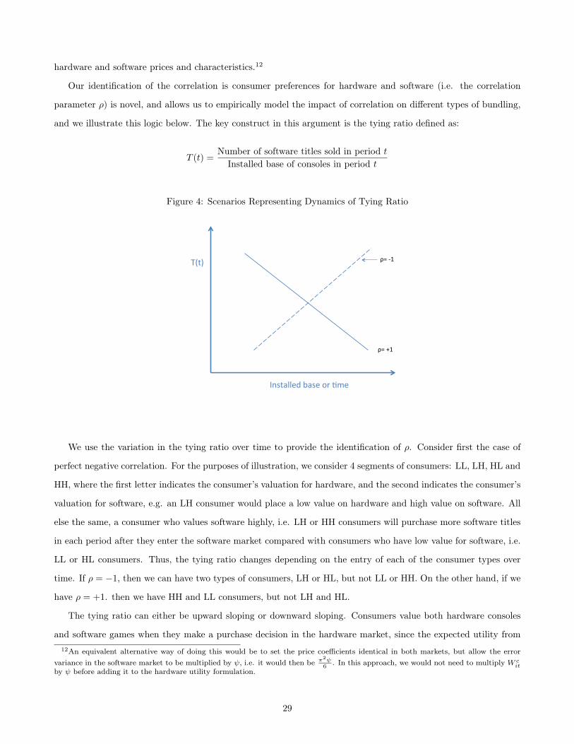
hardware and software prices and characteristics.12
Our identification of the correlation is consumer preferences for hardware and software (i.e. the correlation
parameter ⇢) is novel, and allows us to empirically model the impact of correlation on different types of bundling,
and we illustrate this logic below. The key construct in this argument is the tying ratio defined as:
T (t) =
Number of software titles sold in period t
Installed base of consoles in period t
Figure 4: Scenarios Representing Dynamics of Tying Ratio
T(t)%
Installed%base%or%0me%%%%%%%%%%%%%%%%%%%%%%%%%%
ρ=%41%
ρ=%+1%
We use the variation in the tying ratio over time to provide the identification of ⇢. Consider first the case of
perfect negative correlation. For the purposes of illustration, we consider 4 segments of consumers: LL, LH, HL and
HH, where the first letter indicates the consumer’s valuation for hardware, and the second indicates the consumer’s
valuation for software, e.g. an LH consumer would place a low value on hardware and high value on software. All
else the same, a consumer who values software highly, i.e. LH or HH consumers will purchase more software titles
in each period after they enter the software market compared with consumers who have low value for software, i.e.
LL or HL consumers. Thus, the tying ratio changes depending on the entry of each of the consumer types over
time. If ⇢ = �1, then we can have two types of consumers, LH or HL, but not LL or HH. On the other hand, if we
have ⇢ = +1. then we have HH and LL consumers, but not LH and HL.
The tying ratio can either be upward sloping or downward sloping. Consumers value both hardware consoles
and software games when they make a purchase decision in the hardware market, since the expected utility from12An equivalent alternative way of doing this would be to set the price coefficients identical in both markets, but allow the error
variance in the software market to be multiplied by , i.e. it would then be ⇡2 6 . In this approach, we would not need to multiply W
cit
by before adding it to the hardware utility formulation.
29

software purchases is included in the utility of purchasing the console or bundle. Now consider two cases for the
variation in tying ratio over time in Figure 4. When ⇢ = �1, i.e. the case with HL and LH consumers, consider the
sequence of how these consumers enter the hardware market. If HL enters first followed later by LH, observe that
the tying ratio increases over time, since consumers entering later value software highly and will purchase more
software titles per period than consumers who enter earlier. On the other hand, if LH enters first followed by HL,
then the tying ratio will decrease over time. Thus, the dynamic variation in the tying ratio gives us information
about the sequence of entry of heterogeneous consumers with different valuation for hardware and software.
If ⇢ = +1, i.e. with HH and LL consumers, the only possible entry sequence is the following: HH enters first
followed by LL, in which case the tying ratio is declining over time. Thus, if the tying ratio were increasing over
time, we could infer that ⇢ = �1, whereas with a decreasing tying ratio, we could have two possibilities:
1. ⇢ = +1 and the sequence with HH consumers entering first, followed by LL consumers, or
2. ⇢ = �1 and the entry sequence with LH consumers entering first, followed by HL consumer.
To separate out these two possibilities, we leverage the response of console sales to price variation. We begin with
the idea that HL or HH consumers who value consoles highly are less responsive to price variation in consoles than
LL or LH consumers. Thus, if case (1) above holds, then the HH consumers who enter early are likely to be less
sensitive to price than LL consumers who enter later, implying that the sales response to prices is less sensitive
in early periods and becomes more responsive over time. However, if case (2) above holds, we must find that sales
response to prices is more sensitive in early periods and becomes less responsive over time.
We find from the data that case (1) holds in our setting, consistent with our empirical finding that ⇢ is positive.
More generally, we note that we identify the correlation parameter ⇢ through the combined variation in the tying
ratio and the console sales response to price over time. Note that we have not used any arguments that require
the presence of bundles in the data, and have suggested a rather general identification rationale for correlation in
consumer preferences for two products that are sequentially purchased in a dynamic setting; the rationale relies on
the purchase paths followed by consumers for the two products, i.e. console and videogames in our setting.
The determination of a potential market size for consoles is an important step in properly estimating console
demand. One useful measure which is often used is the number of households with a TV in 2001, since the
introduction of the GBA occurred in 2001. But the GBA is geared toward families with children so the measure
of households with a TV seems to over estimate the potential market size.13 Therefore, we use the number of
households who have children under 18 living at home as the appropriate market, approximately 35.7 million.14
13Dube et al. [2010] and others use a similar approach.14An alternative approach would be to use an approach from Bass (1969) that illustrates how to infer the initial potential market
size of a product from its sales data. "An approximation to the discrete-time version of the model implies an estimation equation inwhich current sales are related linearly to cumulative sales and (cumulative sales)²" (Nair, 2007). Let kt and Kt denote the aggregatesales of all consoles in month t and cumulative sales up to and including month t, respectively. Also, let kt = a + bKt + cK
2t + vt be
the equation we estimate. Given the estimates, the Bass model implies the initial potential market size for all handheld consoles is
30

The potential hardware market in period t includes all consumers who have not made a purchase and remain
in the market in that period. The construction of the potential market size reflects the idea that a consumer is a
first time buyer and does not re-enter the market to purchase additional hardware. Again, it is important to note
that while the discussion here provides intuition for the specific patterns in the data that move parameter values
to vary in magnitude and sign, in practice all the variation in the data is used to estimate each of the parameters,
given the intertemporal substitution possibilities available to consumers, and the linkage between the console and
video game markets.
Estimation
We model heterogeneous consumers, with the consumer’s type drawn from a discrete distribution of Ns
types. The
coefficients are represented by ↵i
= ↵ + ⌫
i
⌃12 . We examine both Monte Carlo simulations in drawing individual-
specific coefficients and then summing over the individuals to obtain a simulation-based approximation, as well as
the quadrature approach [Skrainka and Judd, 2011], which takes a direct polynomial approximation approach to
compute the integral.15 Consistent with the dynamic demand literature, and that of studies of the video game
industry, we set the discount factor to be � = 0.975; however, recent studies have assumed a lower discount factor
in these settings, and demonstrated that consumers discount such purchases by more than the rate implied by a
“market interest rate.”
Our dataset on the videogame industry spans the years 2001-2005. The Nintendo Gameboy Advance (GBA)
introduced in Spring 2001 was a very significant leap in the handheld console market, and began a new generation of
consoles. This feature of the data setting helps us in our estimation process because it mitigates concerns regarding
whether the initial conditions present in the market at the beginning of our data may present persistent effects that
may make accurate estimation of existing consumer inventory more challenging. Having data from the beginning
of a significant market shift also permits us to consider a more tractable state space in the model, which enables
our estimation process to converge in a reasonable time, and permits us to incorporate richer substitution effects
and correlation between consumers’ preferences for hardware and software.
We model the process of market evolution for the hardware and software markets jointly in a consistent manner
that corresponds to aggregate choice behavior of individual consumers, who first purchase a console and then
purchase software games. Given N
s
discrete types of consumers, we denote the sets of consumers of each type to
be S1,S2, . . . ,SNs . The potential market size for hardware in period ⌧ can be captured by the variable Mh(⌧),
M = (a/f), where f is the positive root of the equation f
2+ fb+ ac = 0 and a is from the regression above. We have tried using this
model as an alternative to estimate the market size, and it gives a potential market size of 35.7 million.15 Specifically, we implement a Gaussian-Hermite quadrature approach with five nodes (Ns = 5) to obtain 25 segments from our two
dimensions of heterogeneity.
31

defined as a (N
s
⇥ 1)-vector that captures the number of each of the N
s
types that have not purchased hardware
by the beginning of period ⌧ :
Mh(⌧) =
M1 �
⌧�1X
t=1
m1(t),M2 �
⌧�1X
t=1
m2(t), . . . ,MN
s
�
⌧�1X
t=1
m
N
s
(t)
!
(26)
where m
s
(t) is the number of hardware purchases in period t by consumers in segment s and M
s
is the initial
number of consumers of segment s in period 0. This formalizes the notion that each consumer who purchases a
console or bundle exits the market for hardware. Consumers consequently enter the market for software video
games, and the potential market size of video game purchasers in period t includes consumers who have purchased
consoles across all periods upto and including period ⌧ :
Ms(⌧) =
⌧
X
t=1
m1(t),
⌧
X
t=1
m2(t), . . . ,
⌧
X
t=1
m
N
s
(t)
!
. (27)
Price endogeneity is known to be present for a variety of reasons. For instance, producers may set higher prices
for games with higher quality, where the latter is not observable by the researcher, which will result in the price
coefficients being biased upward. We also include game indicator variables, although with the use of fixed effects,
the proportion of the unobservable product characteristic, which is not accounted for may still be correlated with
price as a result of consumers and producers correctly observing and accounting for the deviation. Under this
assumption, market specific markups will be influenced by the deviation and will bias the estimate of hardware or
software price sensitivity.
In order to accurately estimate and identify a consumer’s price sensitivity for consoles, software and bundles,
we use instrumental variables to correct for endogeneity in prices. We use instruments which serve as proxies
for marginal cost. The instruments for software video game titles include one-month lags of the Japanese to
US exchange rate and the software producer price index. The producer price index is interacted with additional
variables to capture differences between game characteristics, including age, rating and an indicator for integrated
games. Specifically, the software producer price index is interacted with game rating, rating age as well as rating
and an indicator variable for an integrated game. The implementation of such instruments captures and proxies
for variable software costs among newer and older games, game type and quality levels.
Note that new products in most consumer electronics markets are introduced during the holiday season to take
advantage of the higher expected demand. We account for this by using seasonality variables that pick up aggregate
variation during the holiday period. Nevertheless, we acknowledge that strategic timing games played by the firm
have the potential to result in endogeneity and possibly bias the results. We note that this is true in other markets
as well (e.g. Berry et al. [1995] study the market for automobiles where new models are typically introduced in the
32

summer, and Melnikov [2013] and Gowrisankaran and Rysman [2012] examine other consumer electronics markets
where new products are introduced in the holiday season.
Our estimation is based on GMM, and the criterion function gives us the estimator based on the orthogonality
of the unobservable characteristics and the instruments for consoles, games and bundles:16
(↵, ⌃) = argmin
↵,⌃
⇠(↵,⌃); �(↵,⌃); µ(↵,⌃)
�
ZWZ0
2
6
6
6
6
4
⇠(↵,⌃)
�(↵,⌃)
µ(↵,⌃)
3
7
7
7
7
5
. (28)
For hardware, we use a one month lag of the Japanese to US exchange rate again and the retail price of
Nintendo’s home video game console the GameCube as console price instruments. We also include an indicator
variable of whether an additional console type is available (i.e. whether the Gameboy Advance SP has reached
the market) to account for the multi-product pricing effect. The foreign exchange rate is a suitable instrument
given the manufacturing of the console and games occur in Japan and would consequently affect the retail price of
consoles in the US. We employ a one month lag of the exchange rate to allow for the duration between shipping,
displaying and purchasing. Lastly, each instrument is interacted with a console indicator variable for either the
GBA or the GBA SP to allow each variable to enter the production function of each console differently, similar to
Villas-Boas [2007].
Handling the endogeneity of the bundle price is slightly more complicated thanconsoles alone. Given our
model specification where the unobservable bundle characteristic term would involve both hardware and software
characteristics, using only instruments from consoles to instrument for bundle price would still leave our bundle
price correlated with the unobserved term. We correct for the endogeneity problem with the use of both software
and console instruments. We report the first stage results for both software and hardware and an F -test for each
set of excluded instruments in Table 4, to demonstrate that the instruments are appropriate.17
We also supplement our estimation with the use of micro level survey data from Forrester Research’s 2005
Technographics survey. This data allows us to form micromoments based upon the difference between the predicted16 The matrix of instruments is constructed block-diagonally from the instruments for hardware, software and bundles and can be further
specified as:
Z =
2
6664
Z
h0
0 Z
s
Z
hZ
s
3
7775.
17First stage pricing model was jointly estimated given constraint from bundles. We employed the following model:2
4Pg
Pc
Pb
3
5=
2
4xg 0
0 xc
xg xc
3
5⇥
↵g
↵c
�+
2
4zg 0
0 zc
zg zc
3
5⇥
�g
�c
�+ ✏
where x represent product characteristics and z the excluded instruments.
33
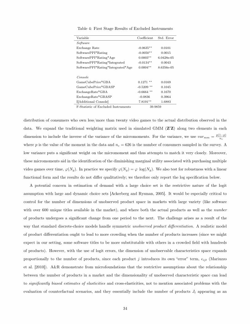
Table 4: First Stage Results of Excluded Instruments
Variable Coefficient Std. ErrorSoftware
Exchange Rate -0.0635⇤⇤ 0.0101SoftwarePPI*Rating -0.0050⇤⇤ 0.0015SoftwarePPI*Rating*Age 0.0003⇤⇤ 6.0428e-05SoftwarePPI*Rating*Integrated -0.0134⇤⇤ 0.0043SoftwarePPI*Rating*Integrated*Age 0.0004⇤⇤ 8.6356e-05
Console
GameCubePrice*GBA 0.1271 ⇤⇤ 0.0169GameCubePrice*GBASP -0.5209 ⇤⇤ 0.1045ExchangeRate*GBA -0.6664 ⇤⇤ 0.1670ExchangeRate*GBASP -0.0836 0.3964I[Additional Console] 7.8191⇤⇤ 1.6883F-Statistic of Excluded Instruments 39.9859
distribution of consumers who own less/more than twenty video games to the actual distribution observed in the
data. We expand the traditional weighting matrix used in simulated GMM (Z0Z) along two elements in each
dimension to include the inverse of the variance of the micromoments. For the variance, we use var
mm
=
p(1�p)n
c
where p is the value of the moment in the data and n
c
= 626 is the number of consumers sampled in the survey. A
low variance puts a significant weight on the micromoment and thus attempts to match it very closely. Moreover,
these micromoments aid in the identification of the diminishing marginal utility associated with purchasing multiple
video games over time, '(Ng
). In practice we specify '(Ng
) = ' log(N
g
). We also test for robustness with a linear
functional form and the results do not differ qualitatively; we therefore only report the log specification below.
A potential concern in estimation of demand with a large choice set is the restrictive nature of the logit
assumption with large and dynamic choice sets [Ackerberg and Rysman, 2005]. It would be especially critical to
control for the number of dimensions of unobserved product space in markets with large variety (like software
with over 600 unique titles available in the market), and where both the actual products as well as the number
of products undergoes a significant change from one period to the next. The challenge arises as a result of the
way that standard discrete-choice models handle symmetric unobserved product differentiation. A realistic model
of product differentiation ought to lead to more crowding when the number of products increases (since we might
expect in our setting, some software titles to be more substitutable with others in a crowded field with hundreds
of products). However, with the use of logit errors, the dimension of unobservable characteristics space expands
proportionally to the number of products, since each product j introduces its own “error” term, ✏ijt
(Mariuzzo
et al. [2010]). A&R demonstrate from microfoundations that the restrictive assumptions about the relationship
between the number of products in a market and the dimensionality of unobserved characteristic space can lead
to significantly biased estimates of elasticities and cross-elasticities, not to mention associated problems with the
evaluation of counterfactual scenarios, and they essentially include the number of products J
t
appearing as an
34
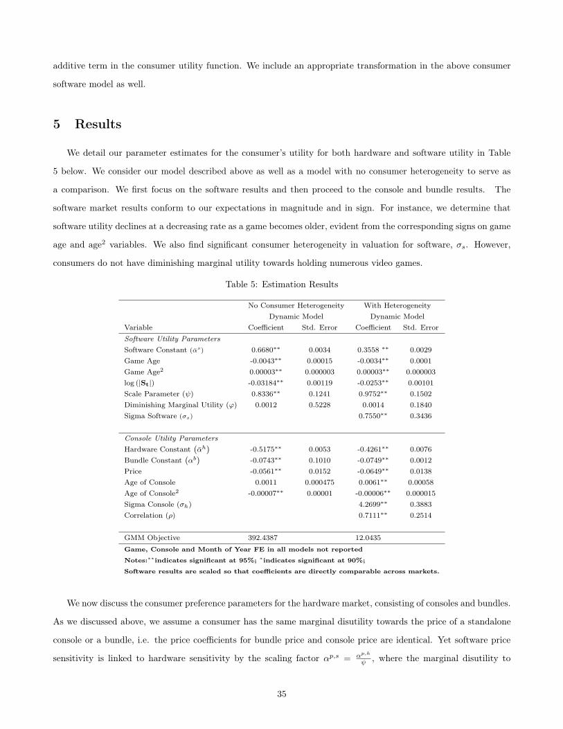
additive term in the consumer utility function. We include an appropriate transformation in the above consumer
software model as well.
5 Results
We detail our parameter estimates for the consumer’s utility for both hardware and software utility in Table
5 below. We consider our model described above as well as a model with no consumer heterogeneity to serve as
a comparison. We first focus on the software results and then proceed to the console and bundle results. The
software market results conform to our expectations in magnitude and in sign. For instance, we determine that
software utility declines at a decreasing rate as a game becomes older, evident from the corresponding signs on game
age and age2 variables. We also find significant consumer heterogeneity in valuation for software, �s
. However,
consumers do not have diminishing marginal utility towards holding numerous video games.
Table 5: Estimation Results
No Consumer Heterogeneity With HeterogeneityDynamic Model Dynamic Model
Variable Coefficient Std. Error Coefficient Std. ErrorSoftware Utility Parameters
Software Constant (↵s) 0.6680⇤⇤ 0.0034 0.3558 ⇤⇤ 0.0029Game Age -0.0043⇤⇤ 0.00015 -0.0034⇤⇤ 0.0001Game Age2 0.00003⇤⇤ 0.000003 0.00003⇤⇤ 0.000003log (|St|) -0.03184⇤⇤ 0.00119 -0.0253⇤⇤ 0.00101Scale Parameter ( ) 0.8336⇤⇤ 0.1241 0.9752⇤⇤ 0.1502Diminishing Marginal Utility (') 0.0012 0.5228 0.0014 0.1840Sigma Software (�
s
) 0.7550⇤⇤ 0.3436
Console Utility Parameters
Hardware Constant�↵
h�
-0.5175⇤⇤ 0.0053 -0.4261⇤⇤ 0.0076Bundle Constant
�↵
b�
-0.0743⇤⇤ 0.1010 -0.0749⇤⇤ 0.0012Price -0.0561⇤⇤ 0.0152 -0.0649⇤⇤ 0.0138Age of Console 0.0011 0.000475 0.0061⇤⇤ 0.00058Age of Console2 -0.00007⇤⇤ 0.00001 -0.00006⇤⇤ 0.000015Sigma Console (�h) 4.2699⇤⇤ 0.3883Correlation (⇢) 0.7111⇤⇤ 0.2514
GMM Objective 392.4387 12.0435Game, Console and Month of Year FE in all models not reported
Notes:
⇤⇤indicates significant at 95%;
⇤indicates significant at 90%;
Software results are scaled so that coefficients are directly comparable across markets.
We now discuss the consumer preference parameters for the hardware market, consisting of consoles and bundles.
As we discussed above, we assume a consumer has the same marginal disutility towards the price of a standalone
console or a bundle, i.e. the price coefficients for bundle price and console price are identical. Yet software price
sensitivity is linked to hardware sensitivity by the scaling factor ↵p,s
=
↵
p,h
, where the marginal disutility to
35

software price is equal to a scaled value of the disutility of hardware price. We determine the scale coefficient
to be statistically significant. We find the hardware price coefficient ↵p,h to be negative and significant as
expected, so that consumers have a marginal disutility toward higher price. Recall that we introduce heterogeneity
in a consumer’s preference for hardware and software. We find that there is a significant degree of consumer
heterogeneity toward consoles (�h
) and that consumer preferences for games and consoles are positively correlated,
and both heterogeneity and correlation are significant. Heterogeneity plays a vital role in the model as consumer
valuation for hardware and software dynamically alters the distribution of consumers who own a console, and who
are therefore present in the software market.
Figure 5: Distribution of (a Sample of) Consumer Types Over Time for the Console Market
0 5 10 15 20 25 30 35 40 450
0.05
0.1
0.15
0.2
0.25
0.3
0.35
Months
Dis
trib
utio
n of
Con
sum
er T
ype
Group 1Group 2Group 3
Figure 5 reflects the distribution of three consumer types over time for the hardware market. In estimation,
we discretize consumers into N
s
= 5 ⇥ 5 = 25 different segments or groups, based on their value for hardware
and software. The fraction of consumers belonging to each specific segment changes dynamically in each market,
depending on consumers’ purchase decisions. Group 1, for instance, is a group which possesses a relatively low
preference for hardware and software. With this low preference consumers within this group postpone consumption
which causes its percentage of consumers who remain in the market for consoles to increase over time (similarly
for Group 2 for the first part of the data period). On the other hand, Group 3 has relatively large preference for
hardware and software and as a result do not postpone consumption into the future as much as groups 1 and 2;
thus, these consumers leave the hardware market earlier, and their numbers subsequently decline over time. Lastly,
we examine whether consumers value bundles over and above the individual products in the bundle (console &
game). We find differences between bundles and consoles. Consumers have a different seasonality effect for bundles
than for consoles.
We next investigate consumer substitution patterns, and Table 6 provides the own and cross price console and
36

Table 6: Console and Bundle Elasticities
GBA GBAMA2 GBAMK SP SPMA4
Gameboy Advance (GBA) 1.09 -0.05 -0.14 -0.48 -0.01
GBA with MarioAdvance2 (GBAMA2) -3.82 4.09 -0.05 -0.01 -0.001
GBA with MarioKart (GBAMK) -4.76 -0.003 9.03 -0.01 -0.001
GBA SP (SP) -0.79 -0.01 -0.01 1.11 -0.06
GBA SP with Mario Adv4 (SPMA4) -1.24 -0.02 -0.01 -4.13 6.01
Note: Cell i,j, where i indexes row and j column, gives the precent change in the total quantity of row i with a one percent change in price of column j
bundle elasticities estimates. We evaluate the elasticity by considering a 1% price cut that is made permanently,
and is known by consumers as well as the firm to be a permanent cut, i.e. there is no uncertainty regarding the
future price cut unlike the case of a limited-time promotion. The model predicts that a permanent 1% percent
reduction in the price of a console would lead to an approximately 1-9% increase in the total number of a given
console sold during the time period. Also note that the own price elasticity for bundles is substantially larger than
for consoles. This result is consistent with previous literature where consumers are more price sensitive to bundles
than components [Sharpe and Staelin, 2010]. The cross-price elasticities correspond to the effect of a price cut
on consoles on sales of bundles, and vice versa and range from 0 to -5%. Moreover, the off-diagonal elements are
negative and the estimated cross-price elasticity measures are consistent with the belief that a standalone console’s
closest “competitor” is the bundle with the particular console included. For instance, the closest “competitor” to
the standalone Gameboy Advance console is the GBA bundle with Mario Advance 2 and not the GBA SP; such a
result would not have been apparent without modeling the microfoundations of consumer demand.
Figure 6 displays the intertemporal handheld console market elasticities. We present three variants of an
elasticity measure to highlight the role of consumer expectations, as is typical in these settings. We compare the
effects of a temporary 1% price decline at time period t when consumers believe the price change is temporary to
one in which consumers believe it is permanent. Our last measure we include is a 1% price decline that is permanent
and is believed to be permanent. In all cases, price changes are not expected in advance by the consumer.
The elasticity measures correspond to the median time period in the data, i.e. month 22. We find that
expectations play a vital role in how consumers respond to price changes. For a temporary and unexpected 1%
price change, we see that sales remain unchanged prior to period t and increase by roughly several percentage points
in that period. We also find that such an unexpected and temporary price change only results in a gain in sales in
the period the price decline is present and a subsequent decline in sales, suggesting inter-temporal substitution by
consumers. However, when the temporary price change is believed to be permanent, we see a smaller reaction in
consumer sales than when the price decline is temporary and believed to be temporary. This is due to consumers’
beliefs that such a price decline in period t will be available next period and so they postpone their purchase until
a future period. But when period (t+ 1) prices return to their higher price levels consumers who otherwise would
37
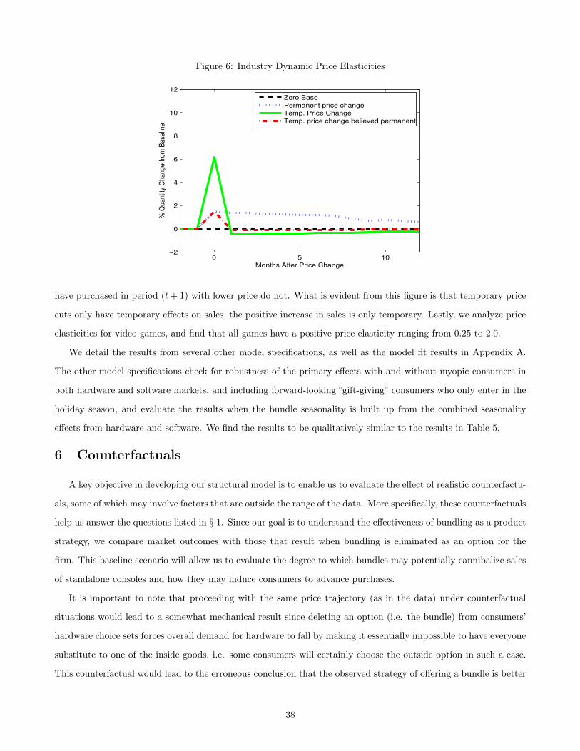
Figure 6: Industry Dynamic Price Elasticities
0 5 10!2
0
2
4
6
8
10
12
Months After Price Change
% Q
uant
ity C
hang
e fr
om B
asel
ine
Zero BasePermanent price changeTemp. Price ChangeTemp. price change believed permanent
have purchased in period (t+ 1) with lower price do not. What is evident from this figure is that temporary price
cuts only have temporary effects on sales, the positive increase in sales is only temporary. Lastly, we analyze price
elasticities for video games, and find that all games have a positive price elasticity ranging from 0.25 to 2.0.
We detail the results from several other model specifications, as well as the model fit results in Appendix A.
The other model specifications check for robustness of the primary effects with and without myopic consumers in
both hardware and software markets, and including forward-looking “gift-giving” consumers who only enter in the
holiday season, and evaluate the results when the bundle seasonality is built up from the combined seasonality
effects from hardware and software. We find the results to be qualitatively similar to the results in Table 5.
6 Counterfactuals
A key objective in developing our structural model is to enable us to evaluate the effect of realistic counterfactu-
als, some of which may involve factors that are outside the range of the data. More specifically, these counterfactuals
help us answer the questions listed in § 1. Since our goal is to understand the effectiveness of bundling as a product
strategy, we compare market outcomes with those that result when bundling is eliminated as an option for the
firm. This baseline scenario will allow us to evaluate the degree to which bundles may potentially cannibalize sales
of standalone consoles and how they may induce consumers to advance purchases.
It is important to note that proceeding with the same price trajectory (as in the data) under counterfactual
situations would lead to a somewhat mechanical result since deleting an option (i.e. the bundle) from consumers’
hardware choice sets forces overall demand for hardware to fall by making it essentially impossible to have everyone
substitute to one of the inside goods, i.e. some consumers will certainly choose the outside option in such a case.
This counterfactual would lead to the erroneous conclusion that the observed strategy of offering a bundle is better
38
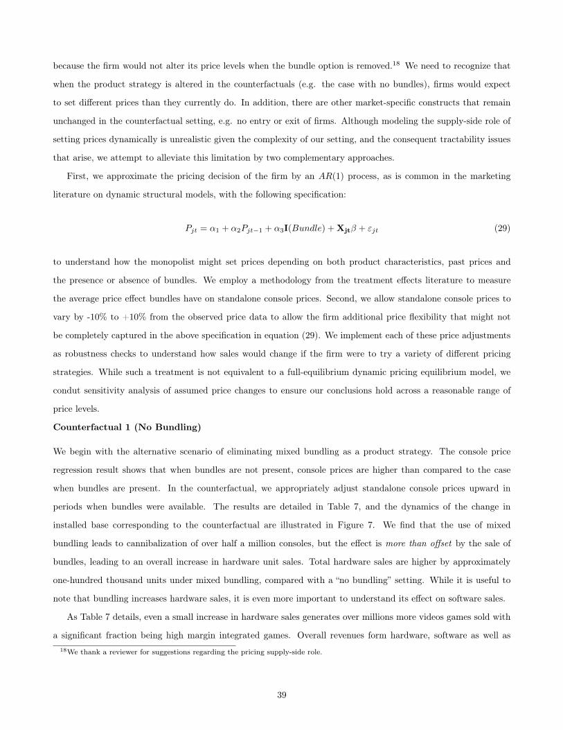
because the firm would not alter its price levels when the bundle option is removed.18 We need to recognize that
when the product strategy is altered in the counterfactuals (e.g. the case with no bundles), firms would expect
to set different prices than they currently do. In addition, there are other market-specific constructs that remain
unchanged in the counterfactual setting, e.g. no entry or exit of firms. Although modeling the supply-side role of
setting prices dynamically is unrealistic given the complexity of our setting, and the consequent tractability issues
that arise, we attempt to alleviate this limitation by two complementary approaches.
First, we approximate the pricing decision of the firm by an AR(1) process, as is common in the marketing
literature on dynamic structural models, with the following specification:
P
jt
= ↵1 + ↵2Pjt�1 + ↵3I(Bundle) +Xjt� + "
jt
(29)
to understand how the monopolist might set prices depending on both product characteristics, past prices and
the presence or absence of bundles. We employ a methodology from the treatment effects literature to measure
the average price effect bundles have on standalone console prices. Second, we allow standalone console prices to
vary by -10% to +10% from the observed price data to allow the firm additional price flexibility that might not
be completely captured in the above specification in equation (29). We implement each of these price adjustments
as robustness checks to understand how sales would change if the firm were to try a variety of different pricing
strategies. While such a treatment is not equivalent to a full-equilibrium dynamic pricing equilibrium model, we
condut sensitivity analysis of assumed price changes to ensure our conclusions hold across a reasonable range of
price levels.
Counterfactual 1 (No Bundling)
We begin with the alternative scenario of eliminating mixed bundling as a product strategy. The console price
regression result shows that when bundles are not present, console prices are higher than compared to the case
when bundles are present. In the counterfactual, we appropriately adjust standalone console prices upward in
periods when bundles were available. The results are detailed in Table 7, and the dynamics of the change in
installed base corresponding to the counterfactual are illustrated in Figure 7. We find that the use of mixed
bundling leads to cannibalization of over half a million consoles, but the effect is more than offset by the sale of
bundles, leading to an overall increase in hardware unit sales. Total hardware sales are higher by approximately
one-hundred thousand units under mixed bundling, compared with a “no bundling” setting. While it is useful to
note that bundling increases hardware sales, it is even more important to understand its effect on software sales.
As Table 7 details, even a small increase in hardware sales generates over millions more videos games sold with
a significant fraction being high margin integrated games. Overall revenues form hardware, software as well as18We thank a reviewer for suggestions regarding the pricing supply-side role.
39

Table 7: Counterfactual 1: Eliminate Bundles
Data Model (Base) CF (No Bundling) Model-CFConsole Sales 25,891,953 25,976,646 26,441,379 -464,733Bundle Sales 563,678 563,886 0 563,886Independent Software Sales 80,845,492 83,270,691 78,088,240 5,182,451Integrated Software Sales 31,400,467 32,308,682 30,311,074 1,997,608Discounted Revenue 2,112,371,134 2,138,564,056 2,087,724,081 50,839,975
overall revenues from mixed bundling are higher than with a component only product strategy.19
We see that bundling is particularly successful in time-shifting purchases of consoles earlier in the life cycle.
Figure 7 depicts the important dynamics of how the hardware installed base under a console only strategy differs
from a mixed bundling strategy. Examining Figure 7b, we find that the consumers who have a low value for
hardware and both low and high value for software are the most impacted by bundling, and accelerate their purchases
when bundles are present in their choice sets. We also find that consumers who have a high value for hardware
are not impacted by the presence of bundling. These results overall suggest that bundling has the potential to
attract lower-valuation segments of consumers to purchase when they might otherwise not do so. It thus provides
an additional mechanism to dynamically segment different types of consumers, and induce substitution from the
‘no purchase’ or ’delay purchase’ options. It is noteworthy that high type consumers do not substitute away
from component products to bundles, since bundles are lower in valuation (and are priced lower than the sum of
component products).
Although the results illustrate an increase in both hardware and software sales from a mixed bundling strategy,
the timing of these additional adoptions is important. A console manufacturer would prefer to sell as much hardware
as early in its life cycle as possible, which results in an increase in software demand due to indirect network effects.
We note that the installed base only considers the benefits of bundling on the hardware market. Thus, if software
producers develop more software when there is a larger installed base, the true effects of bundling are likely to be
even higher than we have documented.19Note that revenues are calculated by summing over three monthly revenues streams with 45 months of data: (i) hardware sales
(bundles and consoles) (ii) royalty fee from independent software sales, which is set at $8 per software title sold, and (iii) revenue fromintegrated games, i.e. those produced by the monopolist firm. Once monthly revenues are calculated, we discount revenues back to thefirst period of the data.
40
Figure 7: Counterfactual 1: Dynamics of Installed Base
(a) Difference in Installed Base with and withoutBundling
0 5 10 15 20 25 30 35 40 450
0.5
1
1.5
2
2.5
3x 10
5
Months
Change in
Inst
alle
d B
ase
(M
ixed B
undlin
g!
Conso
le O
nly
)(b) Consumer Heterogeneity and Bundling Effectiveness
0 5 10 15 20 25 30 35 40 45!0.5
0
0.5
1
1.5
2
2.5
3
3.5
4
Months
Perc
ent C
hange in
Inst
alle
d B
ase
L!Hardware L!SoftwareL!Hardware H!SoftwareH!Hardware L!SoftwareH!Hardware H!Software
Counterfactual 2 (Pure Bundling)
Next, we evaluate the scenario with pure bundling, where consumers must buy a bundle in order to own a console,
i.e. standalone consoles are not available as an option for consumers. Intuitively, pure bundling can be more
profitable when consumers who value either of the component products switch to purchasing the bundle, which can
be positioned to extract higher surplus from consumers, leading to more revenue for the firm. On the other hand,
if consumers switch more to the outside option in the absence of component products, then pure bundling could
result in revenue losses. We note that the literature reviewed in §1 finds support for mixed bundling being more
profitable than pure bundling, as well as the reverse case. We evaluate which effect dominates in our setting, i.e.
do pure bundles increase or decrease revenues? Note that since bundles are not present in every period in the data,
we allow the standalone console to be sold in those periods.
Figure 8 provides the results of the difference between pure and mixed bundling, and we find that mixed bundling
dominates pure bundling with respect to a revenue measure. Given that we do not observe what the bundle price
would be without the pure console, we run our counterfactual simulation for a range of prices, from 10% lower to
10% higher than the bundle price observed in the data. We find that there are highly significant revenue losses
from pure bundling compared with mixed bundling, with differences being at least 35%.
From the first two counterfactuals, we determine that mixed bundling dominates pure components as well as pure
bundling. Our conclusion is based on the role played by dynamics and intertemporal substitution. The firm can
attract consumers who might have only purchased a console in later periods by offering a bundle, which leads those
consumers to purchase bundles earlier. For such a consumer, the bundle is a more compelling value proposition
41
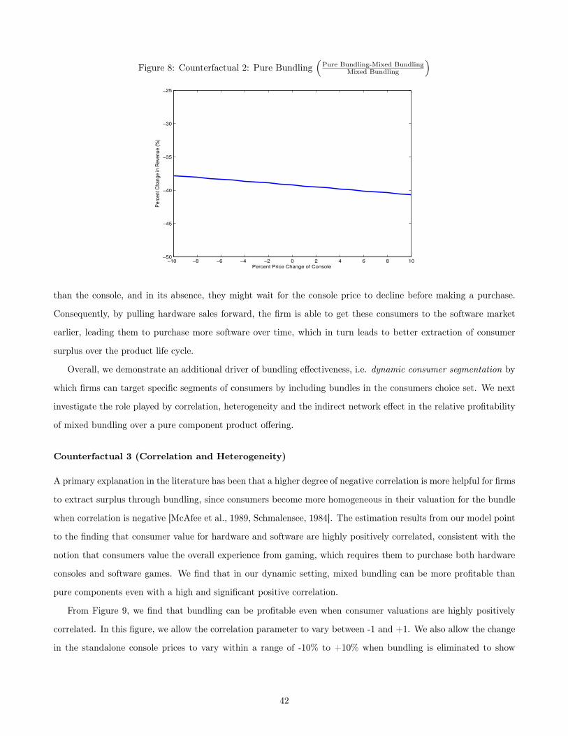
Figure 8: Counterfactual 2: Pure Bundling⇣
Pure Bundling-Mixed BundlingMixed Bundling
⌘
!10 !8 !6 !4 !2 0 2 4 6 8 10!50
!45
!40
!35
!30
!25
Percent Price Change of Console
Per
cent
Cha
nge
in R
even
ue (
%)
than the console, and in its absence, they might wait for the console price to decline before making a purchase.
Consequently, by pulling hardware sales forward, the firm is able to get these consumers to the software market
earlier, leading them to purchase more software over time, which in turn leads to better extraction of consumer
surplus over the product life cycle.
Overall, we demonstrate an additional driver of bundling effectiveness, i.e. dynamic consumer segmentation by
which firms can target specific segments of consumers by including bundles in the consumers choice set. We next
investigate the role played by correlation, heterogeneity and the indirect network effect in the relative profitability
of mixed bundling over a pure component product offering.
Counterfactual 3 (Correlation and Heterogeneity)
A primary explanation in the literature has been that a higher degree of negative correlation is more helpful for firms
to extract surplus through bundling, since consumers become more homogeneous in their valuation for the bundle
when correlation is negative [McAfee et al., 1989, Schmalensee, 1984]. The estimation results from our model point
to the finding that consumer value for hardware and software are highly positively correlated, consistent with the
notion that consumers value the overall experience from gaming, which requires them to purchase both hardware
consoles and software games. We find that in our dynamic setting, mixed bundling can be more profitable than
pure components even with a high and significant positive correlation.
From Figure 9, we find that bundling can be profitable even when consumer valuations are highly positively
correlated. In this figure, we allow the correlation parameter to vary between -1 and +1. We also allow the change
in the standalone console prices to vary within a range of -10% to +10% when bundling is eliminated to show
42
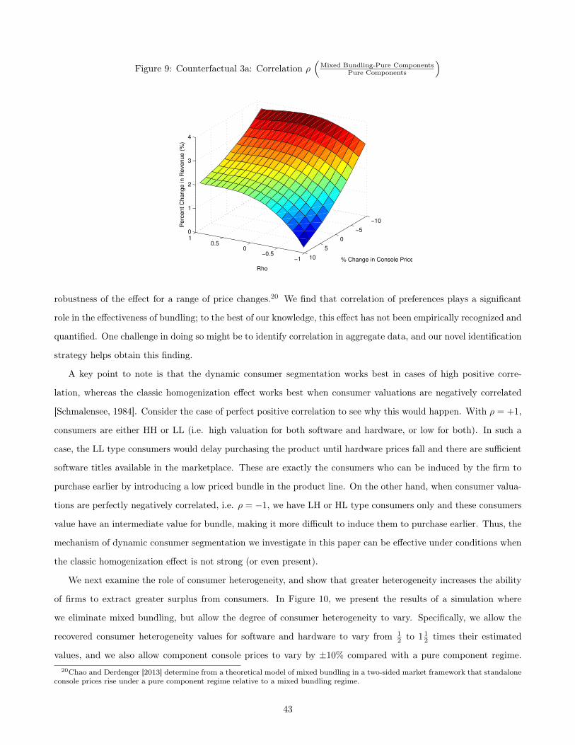
Figure 9: Counterfactual 3a: Correlation ⇢⇣
Mixed Bundling-Pure ComponentsPure Components
⌘
!1!0.5
00.5
1
!10
!5
0
5
10
0
1
2
3
4
% Change in Console Price
Rho
Pe
rce
nt
Ch
an
ge
in R
eve
nu
e (
%)
robustness of the effect for a range of price changes.20 We find that correlation of preferences plays a significant
role in the effectiveness of bundling; to the best of our knowledge, this effect has not been empirically recognized and
quantified. One challenge in doing so might be to identify correlation in aggregate data, and our novel identification
strategy helps obtain this finding.
A key point to note is that the dynamic consumer segmentation works best in cases of high positive corre-
lation, whereas the classic homogenization effect works best when consumer valuations are negatively correlated
[Schmalensee, 1984]. Consider the case of perfect positive correlation to see why this would happen. With ⇢ = +1,
consumers are either HH or LL (i.e. high valuation for both software and hardware, or low for both). In such a
case, the LL type consumers would delay purchasing the product until hardware prices fall and there are sufficient
software titles available in the marketplace. These are exactly the consumers who can be induced by the firm to
purchase earlier by introducing a low priced bundle in the product line. On the other hand, when consumer valua-
tions are perfectly negatively correlated, i.e. ⇢ = �1, we have LH or HL type consumers only and these consumers
value have an intermediate value for bundle, making it more difficult to induce them to purchase earlier. Thus, the
mechanism of dynamic consumer segmentation we investigate in this paper can be effective under conditions when
the classic homogenization effect is not strong (or even present).
We next examine the role of consumer heterogeneity, and show that greater heterogeneity increases the ability
of firms to extract greater surplus from consumers. In Figure 10, we present the results of a simulation where
we eliminate mixed bundling, but allow the degree of consumer heterogeneity to vary. Specifically, we allow the
recovered consumer heterogeneity values for software and hardware to vary from 12 to 1
12 times their estimated
values, and we also allow component console prices to vary by ±10% compared with a pure component regime.20Chao and Derdenger [2013] determine from a theoretical model of mixed bundling in a two-sided market framework that standalone
console prices rise under a pure component regime relative to a mixed bundling regime.
43

Figure 10: Counterfactual 3b: Sigma⇣
Mixed Bundling-Pure ComponentsPure Components
⌘
!50
0
50
!10!5
05
10
1
1.5
2
2.5
3
3.5
4
4.5
% Change in Console Price% Percent Change in Sigma
Pe
rce
nt
Ch
an
ge
in R
eve
nu
e (
%)
We observe that as consumer heterogeneity increases, the value of mixed bundling also increases. Such an increase
in profitability is a direct result of the ability of the bundle to pull consumer sales forward, particularly for those
consumers who do not separately value hardware enough to purchase it on its own early in the life cycle; this
effect in turn leads to more software sales over time. In summary, with a lower degree of heterogeneity among
consumers, the ability to pull sales to earlier periods through the introduction of a bundle is reduced, resulting in
a smaller relative impact of mixed bundling. Taken to the extreme, when all consumers are identical, the dynamic
consumer segmentation effect is highly diminished, and we find that this effect played a significant role in ensuring
the effectiveness of bundling.
Counterfactual 4 (Indirect Network Effect)
Next we examine Counterfactual 4, where we investigate whether an increase in the indirect network effect makes
bundling more or less effective for the firm. We set the marginal benefit of each game for the consumer to increase by
altering the software utility, as included in the hardware utility model. We use a range of one to two times the size
of this effect as recovered from the data, which allows us to determine dynamic comparative statics of the network
effect and mixed bundling. We again allow console prices to vary by ±10% from of the observed console price.
Consumers attach a higher or lower utility to the present discounted utility of software game titles when considering
a hardware purchase in this counterfactual scenario. In Figure 11, we find that a higher network effect decreases
the relative effectiveness of mixed bundling, but does lead to a significant increase in overall discounted revenues.
Moreover, we find that bundling has a smaller effect when the indirect network effect is stronger, suggesting that its
use as a product strategy is likely to be less effective in settings with strong interdependencies between hardware and
software. Thus, we find that bundling could serve as a substitute to network effects rather than as a complement,
44

and expect bundling to be more effectively used in cases where the firm is not able to create a product with strong
network effects. However, there are regions where we allow for significant decline in price changes from the observed
data, where bundling serves as a slight complement to strong network effects. Thus, overall, we would expect the
interaction between bundling and network effects to be more nuanced.
Figure 11: Counterfactual 4: Network Effects⇣
Mixed Bundling-Pure ComponentsPure Components
⌘
!30!20
!100
1020
30
!10!5
05
10
!1
0
1
2
3
4
5
6
% Change in Software Utility% Change in Console Price
Perc
ent
Cha
ng
e in
Reve
nu
e (
%)
7 Discussion, Limitations and Conclusion
We have examined the impact of bundling decisions of firms on consumer choices and market outcomes in a setting
with complementary goods, using data from the handheld video game market consisting of hardware consoles and
software games. Such a setting involves consumer purchases of durable goods that are characterized by indirect
network effects, and where dynamics are especially important. We develop a dynamic model based on individual
consumer behavior, where consumers face a choice of consoles, bundles and video games over time. Consumers
first enter the market for hardware (consoles), and following a hardware purchase, they enter the software (video
games) market. The model allows for forward-looking consumers who have expectations over the future evolution
of hardware and video games, and captures this effect in a tractable manner, building upon recent work on dynamic
demand models. A contribution is that this paper is the first to incorporate the explicit utility from consumer
holdings of a software portfolio into that hardware purchase utility, a framework that we expect to be useful in
many technology and content markets.
We set out to examine how bundling as a product strategy affects sales of consoles (cannibalization) as well
as video games, how bundling creates value through the homogenization effect, and how the presence of indirect
network effects interacts with bundling. We evaluate the mechanisms through which bundling complementary
products creates value for consumers, over and above the valuation for bundle components. First, we find that
bundles ought to be considered as separate products in the product line of a firm, i.e. bundles are not just the same as
putting component products together, i.e. in the terminology of Tellis and Stremersch [2002], we would find bundles
45

in our setting to be product bundles and not price bundles. We find consumer valuation for component products,
i.e. hardware and software, to be positively correlated across the population of consumers. Most importantly, we
identify a new driver of bundling effectiveness, resulting form dynamic consumer segmentation: bundles attract
some segments of consumers to advance their purchases, and others to enter the market when they might not have
otherwise. Note that this is a mechanism that operates independent of the classic “bundling reduces consumer
heterogeneity in valuation” mechanism. We find that the dynamic consumer segmentation explanation allows
bundling to be even mroe effective with positive correlation in consumer valuations for the two products because it
has the power to induce those consumers who have low valuations for both products to intertemporally substitute
purchase to enter the market earlier. On the other hand, the classic homogenization mechanism is likely to be
of limited value, since consumer valuations for component products are positively correlated. The mechanism
of dynamic consumer segmentation underlying the effectiveness of bundling is likely to be especially important
in markets where consumers have heterogeneous valuations for products, and where intertemporal tradeoffs are
especially important, e.g. durable goods or technology products.
We also evaluate whether alternative strategies like pure components or pure bundling may perform more
effectively in place of mixed bundling. We find that console sales diminish in the absence of mixed bundling, and
that consumers who had purchased bundles may not always purchase pure consoles, even though consoles may be
cheaper than bundles. Video game sales drop by millions of units and the overall discounted revenue reduces by
more than fifty million dollars. We find that bundling serves as a substitute to network effects, suggesting it can
be better leveraged when such effects are weaker, and that its relative benefit might not be as much in markets
with strong network or winner-take-all effects. Overall, we find bundling to be a flexible product strategy option,
which allows firms to create entire product lines where only one product existed. While our findings on bundling
are especially true for products with low or zero marginal costs, its effectiveness as a product strategy would be
interesting to examine in other markets.
The study could be enhanced by further work that could address the limitations arising from the nature of
the data and from the viewpoint of computational tractability. First, we develop a model based on individual
consumers with forward-looking behavior, but only have access to aggregate market-level aggregate data. While
this limitation is shared by most empirical studies of durable goods, having access to dis-aggregate individual-level
data would enable us to better examine the heterogeneity in consumer behavior, and could lead to more precise
marketing suggestions. However, we note that to characterize how bundling results in homogenization of valuations
requires aggregate type data, or at least a large sample individual data from a representative set of consumers
sampled across the heterogeneity spectrum.
Second, we do not model the firm’s decision to introduce products at specific time periods (often in the holiday
season as in most consumer electronics markets), which has the potential to bias our findings due to endogeneity
46

constraints. Although we do not model firm decisions as in most dynamic demand models, we instrument for
endogenous pricing and evaluate our findings across a range of counterfactual price levels, and find our results
to hold. Third, from a modeling perspective, we do not allow individual households to purchase hardware in a
repeated manner (they would be treated as different households if they made a repeat hardware purchase). Fourth,
we do not fully model the consumer problem of dynamically choosing the optimal software library or portfolio of
titles, since that would be intractable. Rather, we aim to capture the dynamics in the software market by modeling
decreasing marginal utility for software as well as capturing the dynamic evolution of the software market through
the evolving inclusive value. Fifth, our results may be biased due to limited bundle availability. Suppose that some
consumers did not have bundles in their choice set. Our model assumes all consumers have bundles in their choice
sets when bundles are available, and we find that many consumers choose not to buy bundles when offered the
opportunity. If instead there were limited availability, many consumers would not have bundles in their choice set,
and for consumers who had bundles in their choice set, bundles would receive a higher probability of purchase,
implying they have a higher utility. This would lead us to expect the bundle fixed effect to be less negative that it
currently is in the results. Thus, it has the potential to strengthen the purchase acceleration or dynamic consumer
segmentation, i.e. the mechanism underlying how the firm obtains higher revenue from mixed bundling. We also do
not model the software firms as able to reoptimize their decisions for video games across counterfactuals.21 Finally,
like most other research in this setting, we also abstract away from the used goods market, which has explicitly
been considered only by Ishihara and Ching [2012].
While our results lay the ground for a more empirically grounded understanding of bundling, there remain
several interesting avenues for further research. It would be useful to examine the dynamic introduction and
phase-outs of bundles, including the choice of games to be included in bundles and the choice of whether exclusive
software should be marketed only as part of bundles. Another prospect is to evaluate the competitive dynamics
between firms in introducing bundles, and in characterizing the incentives of third-party game producers to sell
their products bundled with consoles. More broadly, our examination of the role for bundling brings up the issue
of how firms ought to think about product line decisions for individual products when bundling allows them more
flexibility in enabling the creation of differentiated products that can be designed to be temporary or persist for
long periods. Bundling thus can be an effective, practical and profitable component of a firm’s product strategy.
21Although these assumptions create obvious limitations, we argue that we would expect qualitative findings would persist in equi-librium, since they are data-driven and persist across a variety of model specifications, beginning with the assumption of holding standalone software prices constant. If we follow a similar method to analyzing the impact of bundling on component console price as incounterfactual one, we would determine that component prices of bundled software when bundles are not present would decrease by avery small amount. Moreover, given that these video games are bundled late in their life cycle, the increase in pure component revenuerelative to revenue when bundle software prices do not change would be small, leading to the conclusion that the bias associated withour assumption of holding software prices fixed across regimes is rather small.
47

References
D. A. Ackerberg and M. Rysman. Unobserved product differentiation in discrete-choice models: Estimating price
elasticities and welfare effects. RAND Journal of Economics, 36(4):771–788, 2005.
W. J Adams and J. L Yellen. Commodity bundling and the burden of monopoly. The Quarterly Journal of
Economics, 90(3):475–498, 1976.
A. Amelio and B. Jullien. Tying and freebies in two-sided markets. IDEI Working Papers, 2007.
M. Armstrong and J. Vickers. Competitive non-linear pricing and bundling. Review of Economic Studies, 77(1):
30–60, 2010.
Y. Bakos and E. Brynjolfsson. Bundling information goods: Pricing, profits, and efficiency. Management Science,
page 1613–1630, 1999.
S. Berry, J. Levinsohn, and A. Pakes. Automobile prices in market equilibrium. Econometrica, 63(4):841–890,
1995.
B. Caillaud and B. Julien. Competing in network industries: Divide and conquer. RAND J. Econ, 34:309–328,
2003.
J. E. Carranza. Product innovation and adoption in market equilibrium: The case of digital cameras. International
Journal of Industrial Organization, 2010. ISSN 0167-7187.
Y. Chao and T. Derdenger. Mixed bundling in two-sided markets in the presence of installed base effects. Man-
agement Science, 2013.
Y. Chen and M.H. Riordan. Profitability of product bundling. International Economic Review, 54(1):35–57, 2013.
G. Crawford. The discriminatory incentives to bundle in the cable television industry. Quantitative Marketing and
Economics, 6:41–78, 2008.
J. P. Dube, G. J. Hitsch, and P. K. Chintagunta. Tipping and concentration in markets with indirect network
effects. Marketing Science, 29(2):216–249, 2010.
A. Elberse. Bye-Bye bundles: The unbundling of music in digital channels. Journal of Marketing, 74(3):107–123,
2010.
Hanming Fang and Peter Norman. To bundle or not to bundle. The RAND Journal of Economics, 37(4):946–963,
2006.
48

B. R. Gordon. A dynamic model of consumer replacement cycles in the PC processor industry. Marketing Science,
28(5):846–867, 2009.
G. Gowrisankaran and M. Rysman. Dynamics of consumer demand for new durable goods. Journal of Political
Economy, 2012.
G. Gowrisankaran, M. Park, and M. Rysman. Measuring network effects in a dynamic environment. Technical
report, NET Institute Working Paper No. 10, 2010.
A. Hagiu. Pricing and commitment by two-sided platforms. The RAND Journal of Economics, 37(3):720–737,
2006.
W. R Hartmann and H. S Nair. Retail competition and the dynamics of demand for tied goods. Marketing Science,
29(2):366–386, 2010.
I. Hendel and A. Nevo. Measuring the implications of sales and consumer inventory behavior. Econometrica, 74
(6):1637–1673, 2006.
M. Ishihara and A. Ching. Dynamic demand for new and used durable goods without physical depreciation: The
case of japanese video games. Available at SSRN 2189871, 2012.
U. Kaiser and J. Wright. Price structure in two-sided markets: Evidence from the magazine industry. International
Journal of Industrial Organization, 24(1):1–28, 2006.
M. L. Katz and C. Shapiro. Systems competition and network effects. Journal of Economic Perspectives, 8(2):
93–115, June 1994. doi: 10.1257/jep.8.2.93.
B. H Kobayashi. Does economics provide a reliable guide to regulating commodity bundling by firms? a survey of
the economic literature. Journal of Competition Law and Economics, 1(4):707, 2005.
Robin S. Lee. Vertical integration and exclusivity in platform and two-sided markets. American Economc Review,
2013.
F. Mariuzzo, P. P. Walsh, and C. Whelan. Coverage of retail stores and discrete choice models of demand:
Estimating price elasticities and welfare effects. International Journal of Industrial Organization, 28(5):555–578,
September 2010.
R. P. McAfee, J. McMillan, and M. D. Whinston. Multiproduct monopoly, commodity bundling, and correlation
of values. The Quarterly Journal of Economics, 104(2):371–383, 1989.
O. Melnikov. Demand for differentiated durable products: The case of the US computer printer market. Economic
Inquiry, 51(2):1277–1298, 2013.
49

H. Nair. Intertemporal price discrimination with forward-looking consumers: Application to the us market for
console video-games. Quantitative Marketing and Economics, 5:239–292, 2007. ISSN 1570-7156.
H. Nair, P. Chintagunta, and J.P. Dube. Empirical analysis of indirect network effects in the market for personal
digital assistants. Quantitative Marketing and Economics, 2(1):23–58, 2004.
B. Nalebuff. Bundling as an entry barrier. Quarterly Journal of Economics, 119(1):159–187, 2004.
A. Prasad, R. Venkatesh, and V. Mahajan. Optimal bundling of technological products with network externality.
Management Science, 56(12):2224, 2010.
J.C. Rochet and J. Tirole. Two-sided markets: a progress report. The RAND Journal of Economics, 37(3):645–667,
2006.
M. Rysman. Competition between networks: A study of the market for yellow pages. Review of Economic Studies,
71(2):483–512, 2004.
P. Schiraldi. Automobile replacement: a dynamic structural approach. The RAND Journal of Economics, 42(2):
266–291, 2011.
R. Schmalensee. Gaussian demand and commodity bundling. The Journal of Business, 57(1):211–230, 1984.
K.M. Sharpe and R. Staelin. Consumption effects of bundling: Consumer perceptions, firm actions, and public
policy implications. Journal of Public Policy & Marketing, 29(2):170–188, 2010.
B. Skrainka and K. Judd. High performance quadrature rules: How numerical integration affects a popular model
of product differentiation. 2011.
G. Tellis and S. Stremersch. Strategic bundling of products and prices: a new synthesis for marketing. Journal of
Marketing, 66:72, 2002.
R. Venkatesh, V. Mahajan, and V. Rao. The design and pricing of bundles: A review of normative guidelines and
practical approaches. Handbook of Pricing Research in Marketing, Edward Elgar Publishing, Northampton, MA,
pages 232–257, 2009.
S.B. Villas-Boas. Vertical relationships between manufacturers and retailers: Inference with limited data. The
Review of Economic Studies, 74(2):625–652, 2007.
50

Appendix A: Model Fit and Robustness across Specifications
Table 8 presents the seasonally adjusted raw sales data and the model predictions. As the table illustrates, our
above model does quite nicely in predicting console and bundle sales. We determine the model has a prediction
error of 0.44% for hardware and 6.59% for software, which indicates the model over predicts sales. We note that
our prediction errors correspond quite favorably with other results Carranza [2010], Gowrisankaran et al. [2010] .
Table 8: Model Prediction Error
Data Model Prediction ErrorHardware Sales 26,455,631 26,540,532 0.32%Software Sales 112,245,959 115,579,373 2.88%Discounted Revenue 2,112,371,134 2,138,564,056 1.2%
We also assess model fit by reporting the average hardware and software estimation error terms over the 45
month time period. Figure 12 presents this information. From this figure we see no evidence of systematic
auto-correlation or heteroscedasticity of the average hardware or software error term over the time period.
Figure 12: Average Hardware (⇠jt
) and Software (�gt
) Structural Error by Month
5 10 15 20 25 30 35 40 45
!3
!2
!1
0
1
2
3
Months
Hard
ware
Str
uctu
ral E
rror
Te
rm
Zero Base
Mean Hardware Structural Error
5 10 15 20 25 30 35 40 45!2
!1.5
!1
!0.5
0
0.5
1
1.5
2
Months
Softw
are
Str
uctu
ral E
rror
Te
rm
Zero Base
Mean Software Structural Error
Next, we evaluate the robustness of the model to different specifications. We detail the results from four such
specifications in Table 9 below. Note that each of the models below was a dynamic model with forward-looking
consumers, and the estimation approach explicitly recovered consumer heterogeneity. We examined the effect of
changes to our baseline model specification provided in the paper along the following dimensions:
• Bundle specific seasonal effects versus Hardware software seasonal effects: The rationale was to
try and examine whether having separate seasonal effects for the bundle might produce different results than
51

having the bundle seasonality accounted for by the sum of hardware and software seasonal effects.
• Dynamic Hardware: We evaluated the results from model specifications with the introduction of a separate
set of forward-looking consumers in the hardware market. These consumers would enter during the holiday
season (November and December) and not be present in the market during the other months.
• Myopic Software: Building on the baseline model, we investigated whether the presence of the myopic
segment of consumers in the software market actually impacted the results qualitatively. We found that
models with and without myopic consumers tended to produce similar results.
Overall, we find that across a wide range of model specifications, as detailed above, we find that the primary results
of our model are robust, and that the conclusions we report in the main paper follow through across these different
model specifications.
52
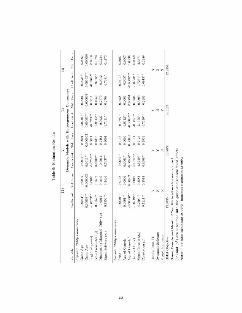
Tabl
e9:
Est
imat
ion
Res
ults
(1)
(2)
(3)
(4)
Dyn
amic
Mod
els
wit
hH
eter
ogen
eous
Con
sum
ers
Var
iabl
eC
oeffi
cien
tSt
d.E
rror
Coe
ffici
ent
Std.
Err
orC
oeffi
cien
tSt
d.E
rror
Coe
ffici
ent
Std.
Err
orSoftware
Utility
Param
eters
Gam
eA
ge-0
.003
4⇤⇤
0.00
01-0
.003
5⇤⇤
0.00
01-0
.003
8⇤⇤
0.00
01-0
.003
5⇤⇤
0.00
01G
ame
Age
20.
0000
3⇤⇤
0.00
0003
0.00
11⇤⇤
0.00
0003
0.00
003⇤
⇤0.
0000
030.
0000
3⇤⇤
0.00
0003
Log
(#of
gam
es)
-0.0
253⇤
⇤0.
0010
-0.0
265⇤
⇤0.
0011
-0.0
277⇤
⇤0.
0011
-0.0
260⇤
⇤0.
0010
Scal
ePar
amet
er(
)0.
9752
⇤⇤0.
1502
0.94
09⇤⇤
0.13
480.
9544
⇤⇤0.
1059
0.97
66⇤⇤
0.15
23D
imin
ishi
ngM
argi
nalU
tilty
(')
0.00
140.
1840
0.00
140.
2481
0.00
220.
2770
0.00
120.
3724
Sigm
aSo
ftw
are(�
s
)0.
7550
⇤⇤0.
3436
0.76
37⇤⇤
0.30
910.
7431
⇤⇤0.
2708
0.74
91⇤
0.41
73
Console
Utility
Param
eters
Pri
ce-0
.064
9⇤⇤
0.01
38-0
.064
9⇤⇤
0.01
43-0
.079
2⇤⇤
0.01
58-0
.071
3⇤⇤
0.01
67A
geof
Con
sole
0.00
61⇤⇤
0.00
060.
0061
⇤⇤0.
0006
0.00
32⇤⇤
0.00
060.
0057
0.00
07A
geof
Con
sole
2-0
.000
06⇤⇤
0.00
002
-0.0
0006
⇤⇤0.
0000
1-0
.000
05⇤⇤
0.00
001
-0.0
0005
⇤⇤0.
0000
2B
undl
eFE(↵
h)
-0.0
749⇤
⇤0.
0012
-0.0
740⇤
⇤0.
0114
-0.0
848⇤
⇤0.
0134
-0.0
720⇤
⇤0.
0069
Sigm
aC
onso
le(�
h)
4.26
99⇤⇤
0.38
834.
5249
⇤⇤0.
7124
2.19
78⇤⇤
0.38
094.
7251
⇤⇤2.
3471
Cor
rela
tion
(⇢)
0.71
11⇤⇤
0.25
140.
6608
⇤⇤0.
2933
0.70
40⇤⇤
0.31
860.
6813
⇤⇤0.
2386
Bun
dle
Tim
eFE
YY
YN
Dya
nam
icSo
ftw
are
NY
NN
Myo
pic
Har
dwar
eN
NY
NG
MM
Obj
ecti
ve12
.043
512
.895
014
.312
712
.825
1G
am
e,C
onsole
and
Month
ofYear
FE
in
allm
odels
not
reported
¯
(↵
s)
and
¯
(↵
h)
are
subsu
med
into
the
gam
ean
dco
nso
lefixe
deff
ects
Notes:
⇤⇤indicates
significant
at
95%
;
⇤indicates
significant
at
90%
;
53
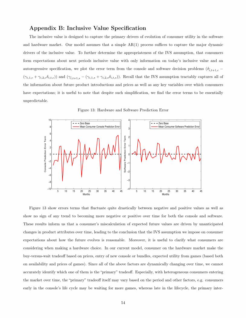
Appendix B: Inclusive Value Specification
The inclusive value is designed to capture the primary drivers of evolution of consumer utility in the software
and hardware market. Our model assumes that a simple AR(1) process suffices to capture the major dynamic
drivers of the inclusive value. To further determine the appropriateness of the IVS assumption, that consumers
form expectations about next periods inclusive value with only information on today’s inclusive value and an
autoregressive specification, we plot the error term from the console and software decision problems (�
i,t+1,c �
(�
i,1,c + �
i,2,c�i,t,c)) and (�
i,t+1,s � (�
i,1,s + �
i,2,s�i,t,s)). Recall that the IVS assumption tractably captures all of
the information about future product introductions and prices as well as any key variables over which consumers
have expectations; it is useful to note that despite such simplification, we find the error terms to be essentially
unpredictable.
Figure 13: Hardware and Software Prediction Error
5 10 15 20 25 30 35 40 45!10
!8
!6
!4
!2
0
2
4
6
8
10
Months
Console
Predic
tion E
rror T
erm
Zero Base
Mean Consumer Console Prediction Error
5 10 15 20 25 30 35 40 45!4
!3
!2
!1
0
1
2
3
4
Months
Softw
are
Pre
dic
tion E
rror
Term
Zero Base
Mean Consumer Software Prediction Error
Figure 13 show errors terms that fluctuate quite drastically between negative and positive values as well as
show no sign of any trend to becoming more negative or positive over time for both the console and software.
These results inform us that a consumer’s miscalculation of expected future values are driven by unanticipated
changes in product attributes over time, leading to the conclusion that the IVS assumption we impose on consumer
expectations about how the future evolves is reasonable. Moreover, it is useful to clarify what consumers are
considering when making a hardware choice. In our current model, consumer on the hardware market make the
buy-versus-wait tradeoff based on prices, entry of new console or bundles, expected utility from games (based both
on availability and prices of games). Since all of the above factors are dynamically changing over time, we cannot
accurately identify which one of them is the “primary” tradeoff. Especially, with heterogeneous consumers entering
the market over time, the “primary” tradeoff itself may vary based on the period and other factors, e.g. consumers
early in the console’s life cycle may be waiting for more games, whereas late in the lifecycle, the primary inter-
54
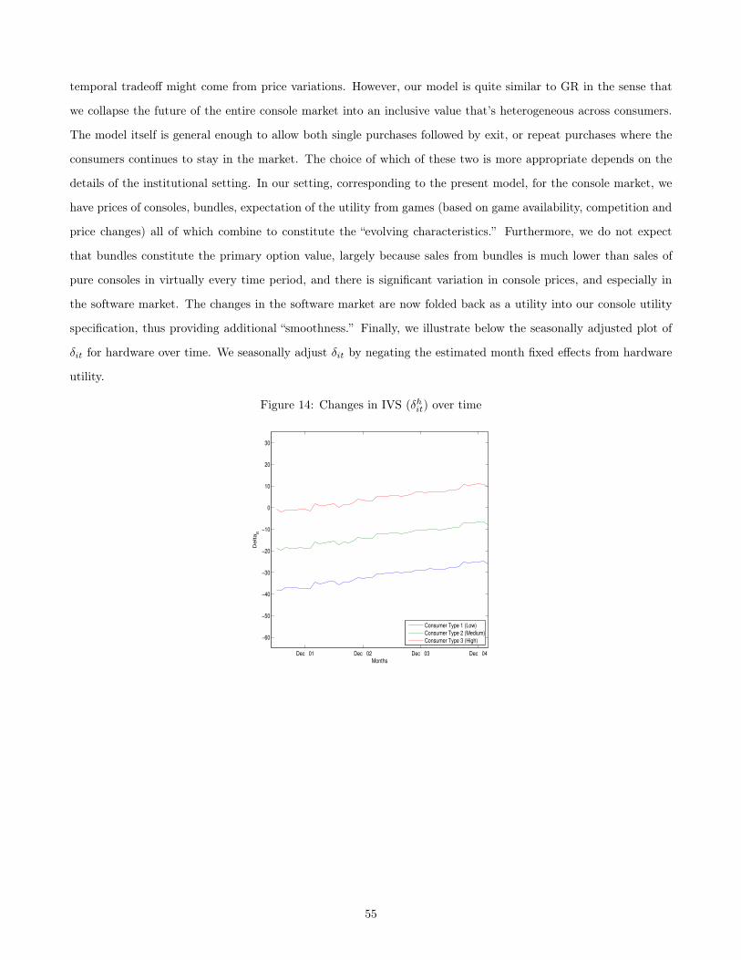
temporal tradeoff might come from price variations. However, our model is quite similar to GR in the sense that
we collapse the future of the entire console market into an inclusive value that’s heterogeneous across consumers.
The model itself is general enough to allow both single purchases followed by exit, or repeat purchases where the
consumers continues to stay in the market. The choice of which of these two is more appropriate depends on the
details of the institutional setting. In our setting, corresponding to the present model, for the console market, we
have prices of consoles, bundles, expectation of the utility from games (based on game availability, competition and
price changes) all of which combine to constitute the “evolving characteristics.” Furthermore, we do not expect
that bundles constitute the primary option value, largely because sales from bundles is much lower than sales of
pure consoles in virtually every time period, and there is significant variation in console prices, and especially in
the software market. The changes in the software market are now folded back as a utility into our console utility
specification, thus providing additional “smoothness.” Finally, we illustrate below the seasonally adjusted plot of
�
it
for hardware over time. We seasonally adjust �it
by negating the estimated month fixed effects from hardware
utility.
Figure 14: Changes in IVS (�hit
) over time
Dec 01 Dec 02 Dec 03 Dec 04
!60
!50
!40
!30
!20
!10
0
10
20
30
Months
De
lta
it
Consumer Type 1 (Low)Consumer Type 2 (Medium)Consumer Type 3 (High)
55

Appendix C: Computational Details
We use the following computational algorithm to begin the GMM procedure that provides a value to the GMM
objective function, given a guess of the parameters: ✓ =�
↵
h
,↵
s
,↵
p,h
,↵
p,s
,↵
x,h
,↵
w,s
,⌃
�
. Note that we set Nmax
=
30.
Overall GMM Objective Procedure:
1. Obtain individual-specific parameters for each hardware and software segment of consumers, i.e.�
↵
h
i
,↵
s
i
�
N
s
i=1
and using quadrature with�
↵
h
,↵
s
,⌃
�
as input. Make initial guess of �hi,t
.
2. Iterate through steps (1) - (15) in the software market procedure until tolerance is reached.
3. Update current estimate of indirect network effect in hardware market, W
s
it
, for each consumer and time
period.
4. Iterate through steps (1) - (9) in the hardware market procedure with current estimate of W
s
it
until
tolerance is reached.
5. Update guess of �hi,t
.
6. Iterate through steps (2) - (5) until tolerance on W
s
it
is reached
7. Compute the GMM objective function defined in equation (28) in the paper.
Software Market Procedure
1. Guess the mean flow utility of games, vsgt
for each g 2 St, and for each period t. For consumer type i, obtain
v
s
igt
= v
s
gt
+ ↵
s
i
.
2. The consumer segment mix is updated recursively for each consumer i and period t as follows:
�
s
i,(t+1) = �
h
i,0 � �
h
i,t
3. Obtain the evolving inclusive value !s
it
for each type of consumer i and period t, using the following equation:
!
s
it
= log
0
@
X
g2St
exp
✓
v
s
igt
1� �
+ ↵
p,g
p
gt
+ hs⌧(t)
◆
1
A
56

4. Obtain the software evolving inclusive value coefficients through estimation of AR(1) regression:
!
s
it+1 = �
s
i,0 + �
s
i,1!s
it
+ ⇣
s
i,t
5. Compute the utility of purchasing each game g 2 St in terms of the evolving inclusive value:
�
s
igt
=
v
s
igt
1� �
+ ↵
p,g
p
gt
+ hs⌧(t) � '(N
g
+ 1) + � E!i
⇥
EV
s
i
(!
s
i,t+1, Ng
+ 1)|!
s
i,t
⇤
6. Compute the total software inclusive value, �sit
based on period utility, flow utility and evolving inclusive
value:
�
s
it
(N
g
) = !
s
it
� '(N
g
+ 1) + � E!i
⇥
EV
s
i
(!
s
i,t+1, Ng
+ 1)|!
s
i,t
⇤
7. Obtain consumer-specific expected value of not purchasing (and continuing) in the software market:
EV
s
i
(!
s
it
, N
g
) = log
⇢
exp
�
!
s
it
� '(N
g
+ 1) + � E!
⇥
EV
s
i
(!
s
i,t+1, Ng
+ 1)|!
s
it
⇤�
| {z }
Purchase
+exp
�
�'(N
g
) + � E!
⇥
EV
s
i
(!
s
i,t+1, Ng
)|!
s
it
⇤�
| {z }
No Purchase
�
where the expectation is taken based on the coefficients recovered through the AR(1) regression above. The
state space is defined as: N
g
2 {1, 2, . . . , N
max
}. Note that when the consumer already holds N
g
� N
max
videogames, then the state continues to be N
max
and is not incremented with a purchase. Thus, the state
transition can more accurately be represented as: N
(t+1)g
= min
n
N
t
g
+
⇣
P
g2S
t
d
gt
⌘
, N
max
o
.
8. Calculate probability of consumer i purchasing in period t:
P
s
it
(�
s
it
, N
g
) =
exp (�
s
it
(N
g
))
exp (EV
s
i
(�
s
it
, N
g
))
9. Calculate the probability of consumer i purchasing product k in period t conditional on making a purchase
as:
P
s
ikt
=
exp(�
s
igt
)
exp (�
s
it
)
.
10. Determine ⇤
it
(N
g
), the fraction of consumers of type i holding N
g
number of games in period t, where
N
g
2 {1, . . . , N
max
}.
11. Compute the forward looking consumer i’s purchase probability share for each product k 2 St in each period
57

t as:
s
dynamic
ikt
= P
s
ikt
0
@
N
max
X
N
g
=0
P
s
it
(�
s
it
, N
g
)⇤
it
(N
g
)
1
A
.
12. If the model has myopic consumers, calculate the myopic consumer i’s purchase probability for each product
k in period t as:
s
myopic
igt
=
exp
⇣
v
s
igt
+ ↵
p,s
p
g,t
+ hs⌧(t)
⌘
1 +
⇣
P
g2Stexp
⇣
v
s
igt
+ ↵
p,s
p
g,t
+ hs⌧(t)
⌘⌘
.
13. The overall market share for product k in period t is determined by integrating out the individual-specific
coefficients, or in a quadrature approach, by weighting appropriately across consumer types (reported results
are from the quadrature approach):
s
kt
= [1� I (seasonalt
)]
X
i2It
�
s
i,t
s
dynamic
ikt
+ I(seasonalt
)
"
2
3
X
i2It
�
s
i,t
s
dynamic
ikt
+
1
3
X
i2It
�
s
i,t
s
myopic
ikt
#
14. Update the flow utilities corresponding to a product-period combination similar to BLP, based on how close
the model is to observed data:
v
s
kt
= v
s
kt
+ log
s
s,DATA
kt
s
s
kt
!
15. Iterate through Steps (3)-(13) until tolerance is reached.
16. Recover the indirect network effect for the hardware market, W c
it
= EV
s
i
(�
s
it
, N
g
= 0) and W
b
it
= EV
s
i
(�
s
it
, N
g
= 1)
.
Hardware Market Procedure
1. Guess F
h
kt
for each k 2 Jt [Bt, and for each period t.
2. Obtain �hikt
for each type of consumer i for each hardware product k and period t, using the following equation:
�
h
ikt
=
8
>
>
<
>
>
:
F
h
kt
+↵h
i
(1��) + ↵
p,h
p
k,t
+ ⌘
h
⌧(t), k 2 Jt
F
h
kt
+↵h
i
+↵s
i
+↵b
(1��) + ↵
p,h
p
k,t
+ ⌘
b
⌧(t),, k 2 Bt
3. Compute the inclusive value for each consumer:
�
h
it
= log
X
k2Jt[Bt
exp
�
�
h
ikt
�
!
58

4. Obtain the hardware coefficients through estimation of AR(1) regression:
�
h
i,t+1 = �
h
i,0 + �
h
i,1�h
i,t
+ ⇣
h
i,t
5. Obtain consumer-specific expected value of not purchasing (and hence continuing) in the hardware market:
EV
h
i
(�) = log
⇣
exp (�) + exp
⇣
� Eh
EV
i
(�
0)|�
i⌘⌘
where the expectation is taken based on the coefficients recovered through the AR(1) regression above.
6. The model-predicted purchase probability share for each product k in each period t is then given for consumer
i to be:
s
h
ikt
=
exp
�
�
h
it
�
⇥
exp
�
EV
h
i
�
�
h
it
��⇤
exp
�
�
h
ikt
�
exp
�
�
h
it
�
7. The overall market share for product k in period t is determined by integrating out the individual-specific
coefficients, or in a quadrature approach, by weighting appropriately across consumer types:
s
h
kt
=
N
s
X
i=1
�
h
i,t
s
h
ikt
8. The consumer segment mix is updated according to the equation, recursively for each consumer i and period
t:
�
i,(t+1) = �
i,t
1�
X
k2Jt[Bt
s
h
ikt
!
9. The flow utilities corresponding to a product-period combination are then updated similar to BLP, based on
how close the model is to the observed data:
F
h
kt
= F
h
kt
+ log
s
h,DATA
kt
s
h
kt
!
10. Iterate through Steps (2)-(9) until tolerance is reached.
59