The Duke Energy Indiana 2018 Integrated Resource Plan July 1, 2019 Volume 1

2

TABLE OF CONTENTS

Chapter/Section Page I. EXECUTIVE SUMMARY 4

A. Overview 4

B. Planning Process Results 7

C. Preferred Portfolio 19

D. Short Term Action Plan 19

E. Long Term Action Plan 19

II. RESOURCE PLANNING PROCESS, METHODS & TOOLS 21

A. Forecasting Methods 21

B. Planning Models 27

C. Resource Screening 28

D. Specifying IRP Objectives 29

E. Scenario Development & Optimized Portfolios 31

F. Alternative Portfolios & Selecting the Preferred Portfolio 33

G. Stakeholder Process 34

III. DUKE ENERGY INDIANA TODAY 36

A. Load and Customer Characteristics 36

B. Current Generating Resource Portfolio 38

C. Current Demand Side Programs 40

IV. DUKE ENERGY INDIANA IN THE FUTURE 42

A. Reference Case Scenario 43

B. Alternative Scenario: Slower Innovation 47

C. Alternative Scenario: High Tech Future 50

D. Alternative Scenario: Current Conditions Persist 53

E. References Case Without Carbon Legislation 55

3

Chapter/Section Page V. CANDIDATE RESOURCE PORTFOLIOS 56

A. Objectives of the 2018 IRP 56

B. Candidate Resources for the 2018 IRP 57

C. Optimized Resource Portfolios 61

D. Sensitivity Analysis 72

E. Alternative Portfolios 78

F. Summary of Candidate Resource Portfolios 87

VI. PREFERRED PORTFOLIO FOR 2018 INTEGRATED RESOURCE PLAN 94

A. Preferred Portfolio 94

B. Short Term Action Plan 97

C. Preferred Portfolios Ability to Adapt to Changing Conditions 97

D. Variables to Monitor and Ongoing Improvements to IRP Process 97

APPENDIX A – Financial & Operating Forecasts for Preferred Portfolio 99

APPENDIX B – Load Forecast 103

APPENDIX C – Supply Side Resources 118

APPENDIX D – Demand Side Resources 134

APPENDIX E – Transmission Planning 171

APPENDIX F – Environmental Compliance 181

APPENDIX G – Cross-Reference to Proposed Rule 194

VOLUME 2 – Summary Document and Stakeholder Meetings (See Volume 2)

4

SECTION I: EXECUTIVE SUMMARY

A. OVERVIEW

Duke Energy Indiana (Company) is Indiana’s largest electric utility, serving approximately

840,000 electric customers in 69 of Indiana’s 92 counties covering North Central, Central, and

Southern Indiana. Its service area spans 22,000 square miles and includes Bloomington, Terre

Haute, and Lafayette, and suburban areas near Indianapolis, Louisville, and Cincinnati.

The Company has a legal obligation and corporate commitment to reliably and economically meet

its customers’ energy needs. Duke Energy Indiana utilizes a resource planning process to identify

the best options to serve customers’ future energy and capacity needs, incorporating both

quantitative analysis and qualitative considerations. For example, quantitative analysis provides

insights into future risks and uncertainties associated with the load forecast, fuel and energy costs,

and renewable energy resource options. Qualitative perspectives, such as the importance of fuel

diversity, the Company’s environmental profile, and the stage of technology deployment are also

important factors to consider as long-term decisions are made regarding new resources. The end

result is a resource plan that serves as an important guide for the Company in making business

decisions to meet customers’ near-term and long-term energy needs.

The resource planning objective is to develop a robust economic strategy for meeting customers’

needs in a dynamic and uncertain environment. Uncertainty is a critical concern when dealing with

emerging environmental regulations, load growth or decline, and fuel and power prices.

Furthermore, particularly in light of the rapidly changing environmental regulations currently

impacting our resource planning process, the Integrated Resource Plan (“IRP” or the “Plan”) is

more like a compass than a road map by providing general direction at this time while leaving the

specific tactical resource decisions to Commission filings using then current information. Major

changes in the 2018 from the 2015 IRP follow.

More Comprehensive Scenarios

The 2018 IRP features five discrete and internally consistent scenarios that enhance analytical

robustness by covering a wider range of possible futures. A consulting firm performed the macro-

5

economic modeling for each scenario using a suite of equilibrium models that defined a set of

internally consistent assumptions. The five scenarios are:

Core Scenarios

1. Slower Innovation

2. Reference Case

3. High Technology

Stakeholder-Inspired Scenarios

4. Reference Case without Carbon Legislation

5. Current Conditions Continue

Uncertainty in a Carbon-Constrained Future

Carbon regulation has been talked about for over a decade and the company has modeled various

levels and forms of regulation. Although much is still not known about how carbon regulation

might be promulgated, the analysis over the last several IRPs has identified it as a major driver for

change in the generating portfolio.

Although the Clean Power Plan has been repealed and the Affordable Clean Energy Rule is

expected to have minimal impact, public sentiment concern about climate change is growing.

Thus, carbon regulation is more a matter of if, than when, and warrants consideration in the plan.

Given the magnitude of the change that would be driven by substantive carbon regulation, a

measured transition towards a less carbon intensive future is prudent.

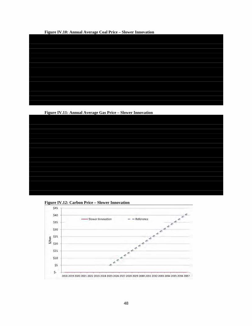
In this IRP, the Company included a price on carbon emissions in the Reference Case scenario of

$5/ton starting in 2025 and growing $3/ton per year to $41/ton by 2037 and in the High Technology

scenario of $10/ton in 2025 increasing $3/ton per year to $47/ton by 2037. This price is a proxy

for potential future legislation addressing carbon emissions.

Our current range of CO2 prices, including a zero price in a number of scenarios, is appropriate

given the outcome of past debates over federal climate change legislation, the uncertainty

6

surrounding future U.S. climate change policy, and that the belief that to be politically acceptable,

climate change policy would need to be moderate. If or when there is additional clarity around

future legislative or regulatory climate change policy, the Company will adjust its assumptions

related to carbon emissions as needed.

Compliance with New EPA Regulations

Additional emerging environmental regulations that will impact the Company’s retirement and

investment decisions include new water quality standards, fish impingement and entrainment

standards, the Coal Combustion Residuals (“CCR”) rule and the new Sulfur Dioxide (“SO2”),

Particulate Matter (“PM”) and Ozone National Ambient Air Quality Standards (“NAAQS”). All

compliance assumptions were reviewed and updated for consistency with other IRP assumptions.

Retirement Analysis

Retirement analysis for the generation fleet was included in overall optimization modeling. The

model optimizes retirement decisions and resource additions simultaneously.

Modeling Energy Efficiency (EE) Programs as Supply Side Resources

Duke Energy Indiana has continued to model EE as a supply-side resource and increased the

number of EE bundles in this IRP to 70 from the 10 bundles in the 2015 IRP. Challenges remain

in how EE is included in the load forecasting process, the uncertainty of EE forecasting, and

combining EE programs into a bundle that can be modeled with supply side resources like natural

gas fired combined cycle or solar resources.

Changes in the Load Forecast

Comparing the 2018 load forecast with 2015, the total energy and peak capacity need for Duke

Energy Indiana decreased across all customer classes primarily due to weak economic growth,

low-cost market power, adoption of federally mandated appliance standards, and energy efficiency

programs. Although long-term trends point toward recovery, energy demand is expected to grow

less than 1% annually for all scenarios.

7

The rest of this Executive Summary presents an overview of the scenarios and portfolios used to

determine the preferred resource plan. Further details regarding the planning process, issues,

uncertainties, and alternative plans are presented in following chapters. See Appendix G for the

location of information required by the Commission’s October 4, 2012 Proposed IRP Rules.

B. PLANNING PROCESS RESULTS

The most prudent approach to address uncertainties is to create a plan that is robust under various

future scenarios. The Company must maintain flexibility to adjust to evolving regulatory,

economic, environmental, and operating circumstances. The planning process includes scenario

analysis. Macro-level driving forces discussed in stakeholder meetings informed the development

of five distinct, internally consistent scenarios.

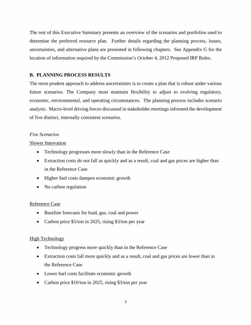
Five Scenarios

Slower Innovation

• Technology progresses more slowly than in the Reference Case

• Extraction costs do not fall as quickly and as a result, coal and gas prices are higher than

in the Reference Case

• Higher fuel costs dampen economic growth

• No carbon regulation

Reference Case

• Baseline forecasts for load, gas, coal and power

• Carbon price $5/ton in 2025, rising $3/ton per year

High Technology

• Technology progress more quickly than in the Reference Case

• Extraction costs fall more quickly and as a result, coal and gas prices are lower than in

the Reference Case

• Lower fuel costs facilitate economic growth

• Carbon price $10/ton in 2025, rising $3/ton per year

8

Reference Case without Carbon Legislation

• Reference Case assumptions except no price on carbon emissions

Current Conditions Continue

• Extrapolations of market curves for gas, coal and power

• Reference Case load forecast

• No carbon regulation

Nine Portfolios

Once the specific modeling assumptions for each scenario were determined, we used a capacity

expansion model to optimize a portfolio for each scenario. We evaluated Nine portfolios organized

into two groups to further increase the robustness of the planning analysis. The first group was

developed as part of the optimization of the assumptions defined by the five scenarios:

Optimized Resource Plans

1. Slower Innovation Portfolio - minimal near-term changes to fleet

2. Reference Case Portfolio - price on carbon drives a couple of coal retirements in 2020s. A

CT and solar are added starting in the mid-2020s

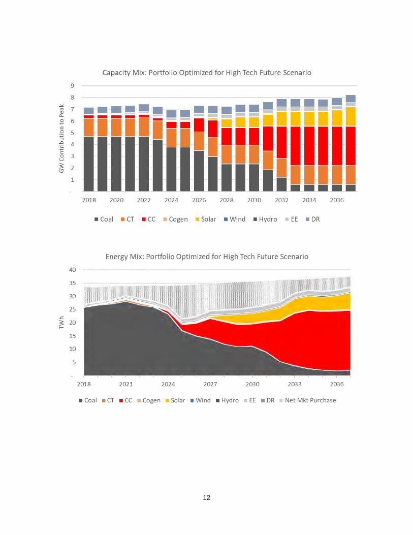
3. High Technology Future Portfolio - a higher price on carbon and lower renewables costs

drive a number of coal retirements in the 2020s; a CC and solar are added starting in the

mid-2020s

4. Reference Case without Carbon Legislation Portfolio - minimal near-term changes to the

fleet

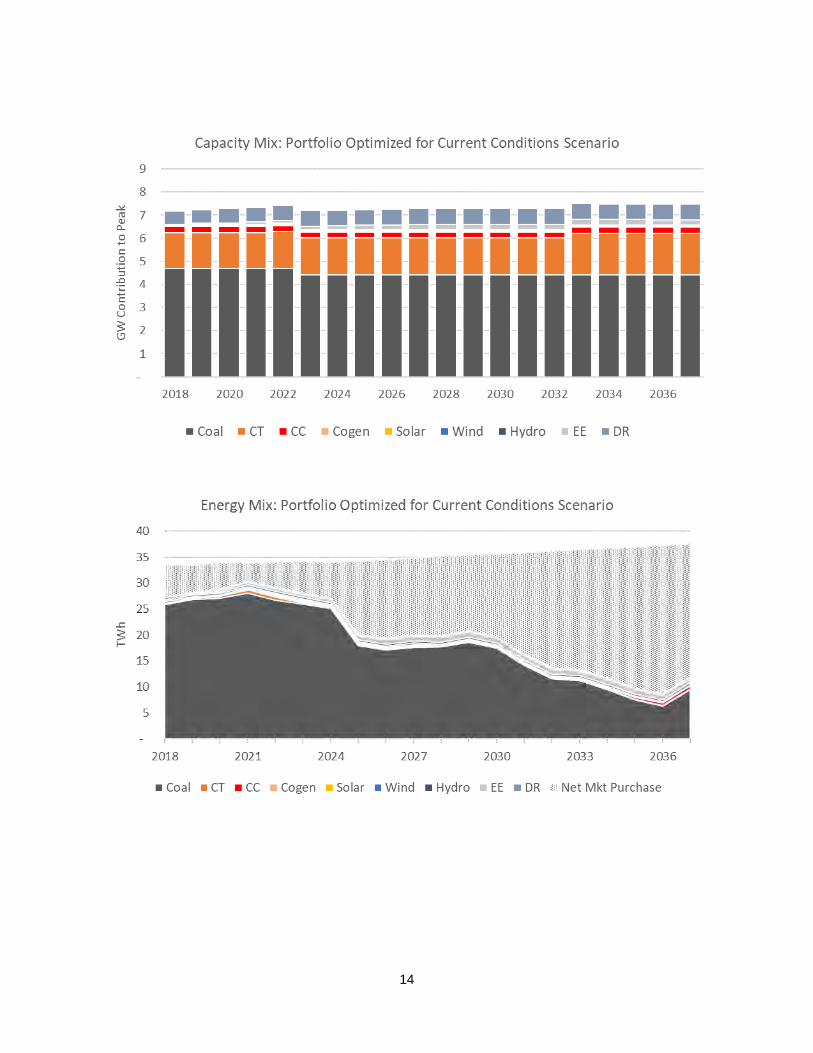
5. Current Conditions Continue Portfolio - minimal near-term changes to the fleet

We developed a group of alternative portfolios by evaluating the optimized portfolios and the

results of sensitivity analysis for lessons learned. The portfolios coming out of that process are:

Alternative Portfolios

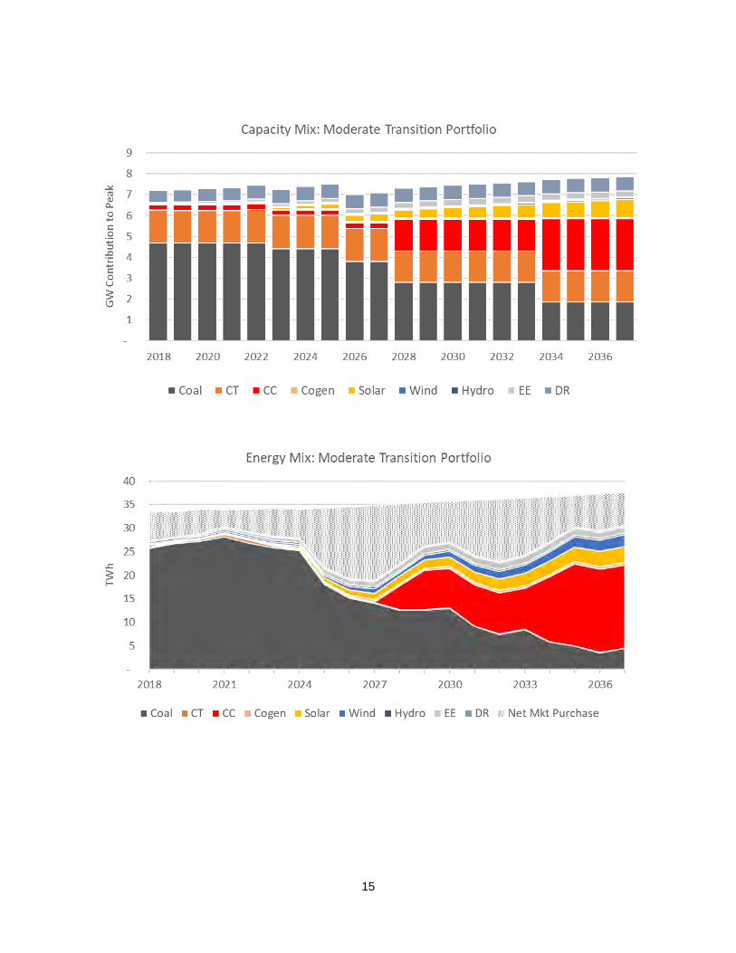
6. Moderate Transition Portfolio - includes three coal unit retirements in the 2020s as well as

a CC with solar and wind additions occurring in the mid/late 2020s

9

7. Aggressive Transition Portfolio - retires Cayuga and Gibson stations (3,800 MW) by the

mid-2030s; adds 3 CCs and solar and wind over time

8. Rapid Decarbonization: CT Portfolio - alters the Aggressive Transition portfolio by

replacing 2 CCs (2480 MW) with more wind, solar and CTs

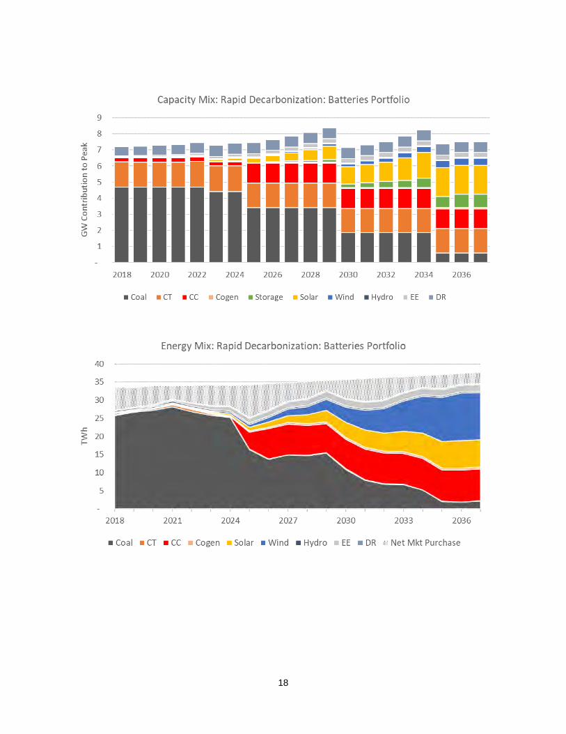
9. Rapid Decarbonization: Batteries Portfolio - alters Aggressive Transition portfolio by

replacing 2 CCs (2,480 MW) with additional wind, solar and storage

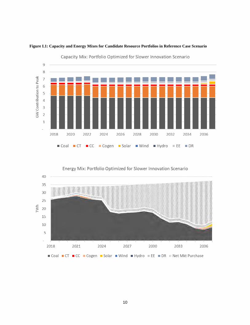
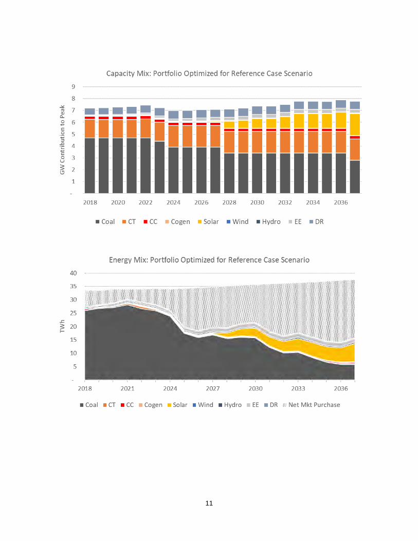
Figure I.1 includes more detail for each portfolio, including how the energy mix in each portfolio

changes over time under the Reference Case scenario.

10

Figure I.1: Capacity and Energy Mixes for Candidate Resource Portfolios in Reference Case Scenario

11

12

13

14

15

16

17

18

19

The objective of the IRP is to produce a robust portfolio that meets the Company’s obligation to

serve load while minimizing the Present Value Revenue Requirements (PVRR) at a reasonable

level of risk, subject to laws and regulations, reliability and adequacy requirements, and

operational feasibility. The selected plan must also meet Midcontinent Independent System

Operator, Inc. (MISO)’s 15.0% reserve margin requirement.

C. PREFERRED PORTFOLIO

Based on its superior performance in scenario and sensitivity analyses, the Moderate Transition

Portfolio was selected by Duke Energy Indiana as the preferred resource plan. This portfolio stands

out due its combination of relatively low cost, lower carbon emissions, greater fuel diversity with

lower exposure to market risk. The Moderate Transition portfolio also has the flexibility to adjust

for different forms of carbon regulation (including no regulation) as well as changing economics

of renewables.

D. SHORT-TERM ACTION PLAN

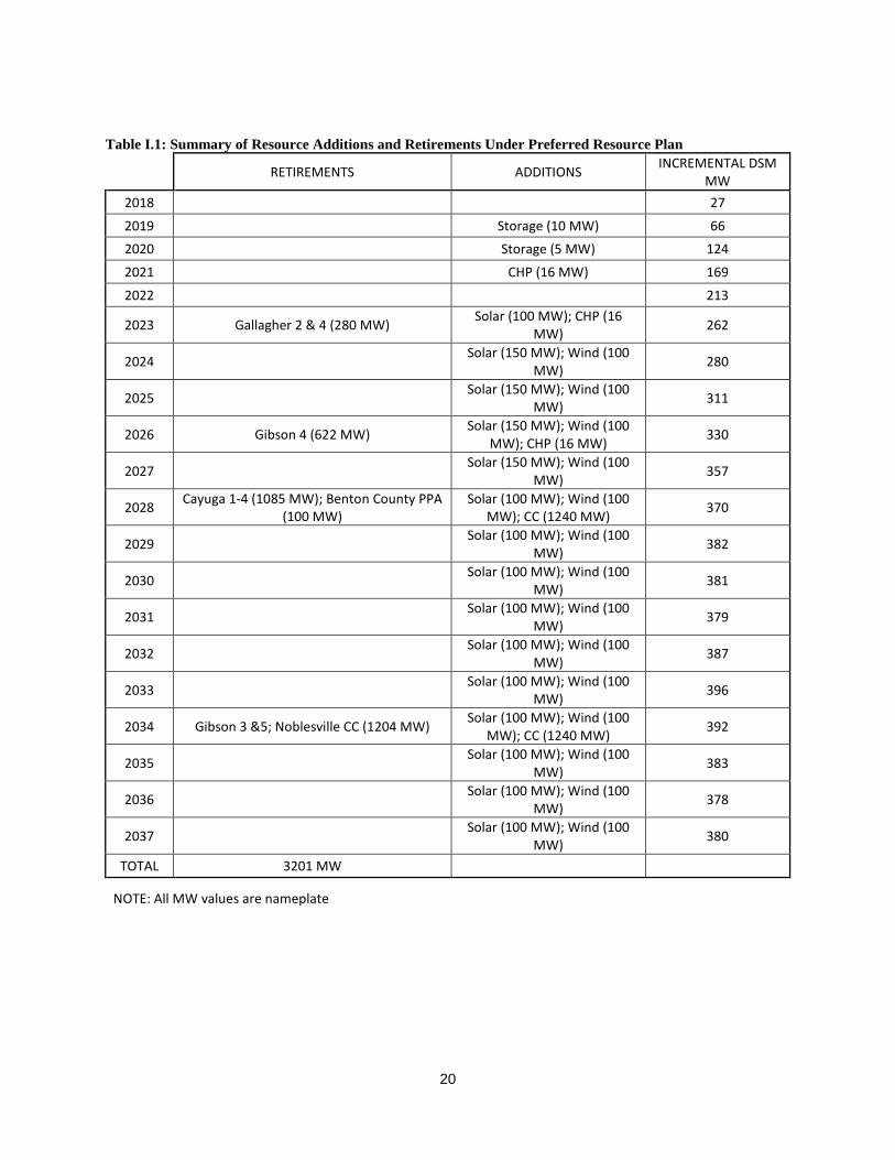
As can be seen in Table I.1, the Moderate Transition Portfolio features a measured approach with

renewable generation progressively added and coal units retired over time. The benefit of this plan

is the flexibility to adjust to changing market and regulatory conditions as well as to smoothly

transition to a more diverse and less carbon intensive fleet.

E. LONG-TERM ACTION PLAN

Longer term, this portfolio can add more renewable if carbon regulation is more stringent or the

cost of renewables decrease more than expected. The Moderate Transition portfolio is better able

to take advantage of low cost gas if that should happen. If carbon regulation is delayed, this

portfolio has the flexibility to adjust its transition. This portfolio takes the Duke Energy Indiana

fleet in a direction with greater flexibility, lower costs, risk and carbon emissions.

20

Table I.1: Summary of Resource Additions and Retirements Under Preferred Resource Plan

RETIREMENTS ADDITIONS INCREMENTAL DSM MW

2018 27

2019 Storage (10 MW) 66 2020 Storage (5 MW) 124

2021 CHP (16 MW) 169

2022 213

2023 Gallagher 2 & 4 (280 MW) Solar (100 MW); CHP (16 MW) 262

2024 Solar (150 MW); Wind (100 MW) 280

2025 Solar (150 MW); Wind (100 MW) 311

2026 Gibson 4 (622 MW) Solar (150 MW); Wind (100 MW); CHP (16 MW) 330

2027 Solar (150 MW); Wind (100 MW) 357

2028 Cayuga 1-4 (1085 MW); Benton County PPA (100 MW)

Solar (100 MW); Wind (100 MW); CC (1240 MW) 370

2029 Solar (100 MW); Wind (100 MW) 382

2030 Solar (100 MW); Wind (100 MW) 381

2031 Solar (100 MW); Wind (100 MW) 379

2032 Solar (100 MW); Wind (100 MW) 387

2033 Solar (100 MW); Wind (100 MW) 396

2034 Gibson 3 &5; Noblesville CC (1204 MW) Solar (100 MW); Wind (100 MW); CC (1240 MW) 392

2035 Solar (100 MW); Wind (100 MW) 383

2036 Solar (100 MW); Wind (100 MW) 378

2037 Solar (100 MW); Wind (100 MW) 380

TOTAL 3201 MW

NOTE: All MW values are nameplate

21

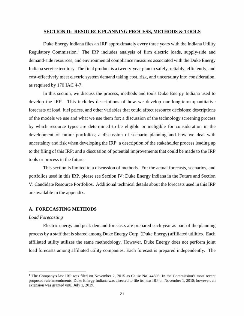
SECTION II: RESOURCE PLANNING PROCESS, METHODS & TOOLS

Duke Energy Indiana files an IRP approximately every three years with the Indiana Utility

Regulatory Commission.1 The IRP includes analysis of firm electric loads, supply-side and

demand-side resources, and environmental compliance measures associated with the Duke Energy

Indiana service territory. The final product is a twenty-year plan to safely, reliably, efficiently, and

cost-effectively meet electric system demand taking cost, risk, and uncertainty into consideration,

as required by 170 IAC 4-7.

In this section, we discuss the process, methods and tools Duke Energy Indiana used to

develop the IRP. This includes descriptions of how we develop our long-term quantitative

forecasts of load, fuel prices, and other variables that could affect resource decisions; descriptions

of the models we use and what we use them for; a discussion of the technology screening process

by which resource types are determined to be eligible or ineligible for consideration in the

development of future portfolios; a discussion of scenario planning and how we deal with

uncertainty and risk when developing the IRP; a description of the stakeholder process leading up

to the filing of this IRP; and a discussion of potential improvements that could be made to the IRP

tools or process in the future.

This section is limited to a discussion of methods. For the actual forecasts, scenarios, and

portfolios used in this IRP, please see Section IV: Duke Energy Indiana in the Future and Section

V: Candidate Resource Portfolios. Additional technical details about the forecasts used in this IRP

are available in the appendix.

A. FORECASTING METHODS

Load Forecasting

Electric energy and peak demand forecasts are prepared each year as part of the planning

process by a staff that is shared among Duke Energy Corp. (Duke Energy) affiliated utilities. Each

affiliated utility utilizes the same methodology. However, Duke Energy does not perform joint

load forecasts among affiliated utility companies. Each forecast is prepared independently. The

1 The Company's last IRP was filed on November 2, 2015 as Cause No. 44698. In the Commission's most recent proposed rule amendments, Duke Energy Indiana was directed to file its next IRP on November 1, 2018; however, an extension was granted until July 1, 2019.

22

load forecast is one of the most important parts of the IRP process. Customer demand provides the

basis for the resources and plans chosen to supply the load.

The general load forecasting framework includes a national economic forecast, a service

area economic forecast, and the electric load forecast. The national economic forecast includes

projections of national economic and demographic concepts such as population, employment,

industrial production, inflation, wage rates, and income. Moody’s Analytics, a national economic

consulting firm, provides the national economic forecast. Similarly, the histories and forecasts of

key economic and demographic variables for the service area economy are obtained from Moody’s

Analytics. The service area economic forecast is used together with the energy and peak demand

models to produce the electric load forecast. In addition, the company conducts customer surveys

every three to five years to determine end-use electricity consumption patterns.

Energy sales projections are prepared for the residential, commercial, industrial, street

lighting, and public authority sectors. Sales projections and electric system losses are combined to

produce a net energy forecast. These forecasts provide the starting point for the development of

the IRP. For additional technical details and data, please see Appendix B.

Forecasting Fuel Prices

The Company uses a combination of observable forward market prices and long-term

commodity price fundamentals to develop coal and gas price forecasts. The former incorporate

data from public exchanges including NYMEX, as well as fuel contracts and price quotes from

fuel providers in response to regular Duke Energy fuel supply requests for proposals. The long-

term fundamental fuels forecast is a proprietary product developed by IHS Markit Ltd., a leading

energy consulting firm2. Fuel price forecasts provided by IHS are based on granular, integrated

supply/demand modeling using fuel production costs and end-user consumption. The Duke Energy

long-term fundamental forecast is approved annually by Duke Energy's leadership for use in all

long-term planning studies and project evaluations.

2 This content is extracted from the IHS Markit North American Power, Gas, Coal and Renewables service and was developed as part of an ongoing subscription service. No part of this content was developed for or is meant to reflect a specific endorsement of a policy or regulatory outcome. The use of this content was approved in advance by IHS Markit. Any further use or redistribution of this content is strictly prohibited a without written permission by IHS Markit. Copyright 2018, all rights reserved.

23

The development of plausible high and low-price fuel forecasts is necessary to enable

creation of a range of future scenarios for long range resource planning. To accomplish this, the

Company’s long-term fundamental fuel forecasts were adjusted using forecast factors from the

Energy Information Administration’s (EIA) Annual Energy Outlook (AEO). The forecast factors

used for low fuel price development are from the AEO 2018 High Oil and Gas Resource and

Technology Case and the factors for high fuel price development are from the AEO 2018 Low Oil

and Gas Resource and Technology Case. These high and low fuel forecasts will be shown in

greater detail in the scenario descriptions in Section IV of this Document.

Fuel Supply Considerations

Duke Energy Indiana generates energy to serve its customers through a diverse mix of fuels

consisting primarily of coal, natural gas, and fuel oil; it also participates in the MISO power

market, which encompasses a variety of generation sources in parts of 15 U.S. states and the

Canadian province of Manitoba. The Company continues to generate a majority of its energy

using coal, with usage dictated by the relative prices of coal as compared to the fuel alternatives

in the economic dispatch process.

Coal

Over 90% of Duke Energy Indiana’s total energy is generated from burning or gasifying

coal. In evaluating the purchase of coal, the Fuels Department considers three primary factors: (1)

the reliability of supply in quantities sufficient to meet Duke Energy Indiana generating

requirements, (2) the quality required to meet environmental regulations and/or manage station

operational constraints, and (3) the lowest reasonable cost as compared to other purchase options.

The “cost” of the coal as evaluated by the Fuels Department includes the purchase price at the

delivery point, transportation costs, scrubbing costs for sulfur, and the evaluated economic impacts

of the coal quality on station operations.

To aid in fuel supply reliability, fuel procurement policies (such as contract versus short

term ratios or inventory target levels) guide decisions on when the Fuels Department should enter

the market to procure certain quantities and types of fuel. These policies are viewed in the context

of economic and market forecasts and probabilistic dispatch models to collectively provide the

24

Company with a five-year strategy for fuel purchasing. The strategy provides a guide to meet the

goal of having a reliable supply of low cost fuel.

To enhance fuel supply reliability and mitigate supply risk, Duke Energy Indiana purchases

coal from multiple mines in the geographic area of our stations. Stockpiles of coal are maintained

at each station to guard against short-term supply disruptions. Currently, coal supplied to the base

load coal stations comes primarily from Indiana and Illinois. These states are rich in coal reserves

with decades of remaining economically recoverable reserves. In 2018, over 95% of the coal

supplied to base load stations was under long-term coal contracts.

Prior to entering long-term commitments with coal suppliers, the Company evaluates the

financial stability, performance history and overall reputation of potential suppliers. By entering

into long-term commitments with suppliers, Duke Energy Indiana further protects itself from risk

of insufficient coal availability while also giving suppliers the needed financial stability to allow

them to make capital investments in the mines and hire the labor force. If the Company were to

try to purchase significant portions of its requirements on the short-term open market, the

Company likely would have severe difficulties in finding sufficient coal for purchase to meet our

needs due to the inability of the mines to increase production to accommodate the 10-12 million

annual tons of coal the Duke Energy Indiana typically consumes in such a short timeframe.

The current Duke Energy Indiana supply portfolio includes nine long-term coal supply

agreements. Under these contracts, the Company buys coal at the mine. Thus, the contracts do

not restrict our ability to move the coal to the various Duke Energy Indiana coal-fired generating

stations as necessary to meet generation requirements. This arrangement allows for greater

flexibility in meeting fluctuations in generating demand and any supply or transportation

disruptions.

For the low capacity factor Gallagher coal station, a much shorter-term procurement policy

is used due to the planned retirement of these aging units. Generally, we source lower-sulfur coal

for these intermediate units on a short-term basis, typically one-year or less, from such places as

Colorado, Wyoming, Indiana and West Virginia.

Duke Energy Indiana fills out the remainder of its fuel needs for both base load and

intermediate load stations with spot coal purchases. Spot coal purchases are used to 1) take

advantage of changing market conditions that may lead to low-priced incremental tonnage, 2) test

25

new coal supplies, and 3) supplement coal supplies during periods of increased demand for

generation or during contract delivery disruptions.

Natural Gas

The use of natural gas by Duke Energy Indiana for electric generating purposes has

generally been limited to CT and CC applications. Natural gas is currently purchased on the spot

market and is typically transported (delivered) using interruptible transportation contracts or as a

bundled delivered product (spot natural gas plus transportation), although the company does have

firm transportation contracts as follows: (1) Midwestern Gas pipeline for gas delivery to

Edwardsport, Vermillion, and Wheatland, and 2) Panhandle Eastern Pipeline for delivery to

Noblesville. The modeled future CC fuel cost incorporates both the natural gas commodity price

and firm transportation cost, and the modeled future CT fuel cost includes the natural gas

commodity price and interruptible transportation cost.

Oil

Duke Energy Indiana uses fuel oil for starting coal-fired boilers and for flame stabilization

during low load periods. Cayuga Unit CT4 uses oil as a back-up fuel. Oil supplies, are purchased

on an as-needed basis, and are expected to be sufficient to meet needs for the foreseeable future.

Forecasting Power Prices

As with fuel prices, we combine near-term observable market prices and long-term

fundamental projections to develop power price forecasts. The Company uses PROMOD to

develop long-term fundamental power price projections based on scenario-specific fuel price

forecasts, a scenario specific generation resource mix for the Eastern Interconnect, and carbon

price assumptions. PROMOD incorporates this information and simulates the dispatch of regional

power markets to develop a power price forecast for Duke Energy Indiana. We use this method

to ensure consistency and provide a linkage between fuel, carbon, and power price assumptions.

To better calibrate the way in which dispatch model replicates making real-world generating unit

commitment decisions, the IRP dispatch model is not permitted to purchase energy from the

market unless the wholesale power price forecast is at least $2/MWh greater than the forecasted

marginal cost of energy from company-owned resources.

26

Forecasting Prices for Carbon Emissions

In the current legislative/regulatory environment it is very difficult to project what a

carbon-constrained future will look like. However, the Company believes that a constraint or price

on carbon is likely to be imposed at some future date, so it is prudent to incorporate such a

constraint into our resource planning. To that end, Duke Energy used an iterative modeling process

to develop a forecast of the CO2 allowance price trajectory that would be required to achieve

reductions in CO2 emissions of 40% by 2030 and 60% by 2050 across the regulated enterprise

(DEI, Duke Energy Kentucky, Duke Energy Carolinas, Duke Energy Progress, and Duke Energy

Florida).

Forecasting Capital Costs

Duke Energy, in conjunction with a third party, developed capital cost projections for all

generation technologies included in the IRP optimization models. These projections are based on

Technology Forecast Factors from the EIA’s Annual Energy Outlook (AEO) 2018. The AEO

provides costs projections for various technologies through the planning period as an input to the

National Energy Modeling System (NEMS).

Using 2018 as a base year, an "annual forecast factor is calculated based on the

macroeconomic variable tracking the metals and metal products producer price index, thereby

creating a link between construction costs and commodity prices." (NEMS Model Documentation

2016, July 2017)

From NEMS Model Documentation 2016, July 2017:

"Uncertainty about investment costs for new technologies is captured in the

Electric Capacity Planning module of NEMS (ECP) using technological optimism

and learning factors.

• The technological optimism factor reflects the inherent tendency to

underestimate costs for new technologies. The degree of technological

optimism depends on the complexity of the engineering design and the

stage of development. As development proceeds and more data become

available, cost estimates become more accurate and the technological

optimism factor declines.

27

• Learning factors represent reductions in capital costs due to learning-

by-doing. Learning factors are calculated separately for each of the

major design components of the technology. For new technologies, cost

reductions due to learning also account for international experience in

building generating capacity. Generally, overnight costs for new,

untested components are assumed to decrease by a technology specific

percentage for each doubling of capacity for the first three doublings,

by 10% for each of the next five doublings of capacity, and by 1% for

each further doubling of capacity. For mature components or

conventional designs, costs decrease by 1% for each doubling of

capacity."

To develop a more accurate forecast for rapidly developing technologies such as solar PV

and battery storage, we blended the AEO forecast factors with additional third-party capital cost

projections. See Appendix C for all capital cost projections.

B. PLANNING MODELS

System Optimizer (SO) is an economic optimization model used to develop IRPs while

satisfying reliability criteria. The model assesses the economics of various resource investments

including conventional generating units such as CTs, CCs, coal units, or IGCC and renewable

resources such as wind or solar. SO uses a linear programming optimization procedure to select

the most economic expansion plan based on Present Value Revenue Requirements (PVRR). The

model calculates the cost and reliability effects of modifying the load with DSM programs or

adding supply-side resources to the system.

Planning and Risk (PAR) is a detailed production-cost model for simulation of the optimal

operation of an electric utility’s generation facilities. Key inputs include generating unit data, fuel

data, load data, transaction data, Demand Side Management (DSM) data, emission and allowance

cost data, and utility-specific system operating data.

PROMOD is a fundamental electric market simulation solution that incorporates extensive

details in generating unit operating characteristics, transmission grid topology and constraints, and

market system operations. A generator and portfolio modeling system, PROMOD, provides nodal

locational marginal price (LMP) forecasting and transmission analysis.

28

C. RESOURCE SCREENING

Supply-Side Resources

Supply-side resources may include existing generating units; repowering options for these

units; potential bilateral power purchases from other utilities, Independent Power Producers (IPPs)

and combined heat and power applications; short-term energy and capacity transactions within the

MISO market; and new utility-built generating units (conventional, advanced technologies, and

renewables). When considering these resources for inclusion in the portfolio, the Company

assesses their technical feasibility, commercial availability, fuel availability and price, useful life

or length of contract, construction or implementation lead time, capital cost, operations and

maintenance (O&M) cost, reliability, and environmental impacts.

The first step in the screening process for supply-side resources is a technical screening to

eliminate from consideration those technologies that are not both technically and commercially

available to the Company. Also excluded from further consideration are technologies that are not

feasible, available or economically viable in or near the Duke Energy Indiana service territory.

Supply-side resources not excluded for availability reasons are included as potential options in the

economic optimization modeling process using the SO model.

Additional details on the screening of supply-side resources can be found in Appendix C.

Retirement Analysis

Generating unit retirements are selected in the System Optimizer (SO) model using a three-step

process. This is necessary because fixed costs are an input to SO, and the model does not calculate

these costs in an iterative fashion. The steps include two SO runs and an intermediate step in

which future fixed costs are forecast using a separate tool.

1. An initial SO run is conducted in which the system is modeled over the planning period

with no units eligible for retirement. The key output of this run is the capacity factor of

each unit in each year of the planning period.

2. A spreadsheet tool is used to forecast future maintenance cycles, capital expenditures for

maintenance, and fixed operating costs, all based on forecasted run hours (capacity factors)

from the initial SO run. These fixed cost forecasts for each unit are used as an input for a

second SO run.

29

3. The second SO run is conducted using the fixed cost forecasts from Step 2 as an input. All

other inputs are identical to the initial run. In this final run, SO selects units for retirement

when the present value of future fixed and variable costs exceeds the costs associated with

retirement and replacement. That is, if the costs that can be avoided by retiring a unit are

greater than the cost of running the system without that unit (including the cost of

replacement), then the unit is retired.

Note that the cost of replacing a unit is never as simple as a one-for-one replacement of megawatts

based on capital cost. Costs may include new capacity from a variety of sources as well as changes

to the dispatch of existing units, and these changes may be realized over multiple years.

Furthermore, total replacement capacity will not equal the capacity of the retiring unit due to

differences in unit size and changes to peak load over time. The SO model considers all of these

factors and their interdependencies over the planning period when selecting resource retirements

and additions.

Demand-Side Resources

The Company received approval for its 2017-19 EE portfolio under Cause No. 43955

DSM-4 and is currently implementing that portfolio for 2019. For the purpose of this IRP, the EE

forecast is based on the implementation of the portfolio approved in Cause No. 43955 DSM-4 and

assumptions for future EE forecasts are based on this portfolio (for 2020) along with information

provided in a recent Market Potential Study conducted by Nexant for periods beyond

2020. Further details of the methodology used to forecast beyond 2019 are included in Appendix

D.

D. SPECIFYING IRP OBJECTIVES

The purpose of this IRP is to define a robust strategy to furnish electric energy services to

Duke Energy Indiana customers in a reliable, efficient, economic manner in accordance with all

applicable environmental regulations while remaining dynamic and adaptable to changing

conditions. We use scenario planning and sensitivity analysis to address areas of regulatory,

economic, environmental, and operating uncertainty. The triennial filing schedule allows the

Company to monitor key sources of uncertainty and adjust the plan as necessary, thereby

30

producing an IRP that represents the most reliable and economic path forward based upon robust

analysis of emerging information.

Our long-term planning objective is to develop a resource strategy that considers the costs

and benefits to all stakeholders (customers, shareholders, employees, suppliers, and community)

while maintaining the flexibility to adapt to changing conditions. At times, this involves striking a

balance between competing objectives.

Determining a Planning Reserve Margin

We address system reliability and resource adequacy in the planning process by targeting

an appropriate planning reserve margin for use in our IRP models. Duke Energy Indiana’s reserve

requirements are driven by ReliabilityFirst, which has adopted a Resource Planning Reserve

Requirement Standard that the Loss of Load Expectation (LOLE) due to resource inadequacy

cannot exceed one day in ten years (0.1 day per year). This Standard is applicable to the Planning

Coordinator, which is MISO for Duke Energy Indiana.

Planning Reserve Margin (PRM) can be expressed on either an ICAP (i.e., installed capacity)

or UCAP (i.e., unforced capacity) basis. The required MISO PRMICAP is translated to PRMUCAP

using the MISO system average equivalent forced outage rate excluding events outside of

management control (XEFORd)3 and assigned to each load serving entity (LSE) on a UCAP basis.

For the 2018/19 Planning Year, the Company is required to meet a PRMUCAP of 8.4%.

Duke Energy Indiana’s IRP models utilize the full installed capacity (ICAP) unit ratings to

estimate dispatch so the MISO assigned PRMUCAP is translated to an equivalent Installed Capacity

(PRMICAP) target which is the historical method used by the Company for modeling purposes. For

Planning Year 2018/19, the applicable RMICAP is 17.9%.4 Because the RMICAP derived from

MISO’s PRMUCAP fluctuates annually, Duke Energy Indiana selects a longer-term planning

reserve margin near the midpoint of recent MISO annual requirements. The long-term ICAP

planning reserve margin utilized for the 2018 integrated resource plan is 15.0%.

3 PRMUCAP = (1 – MISO Average XEFORd)(1 + PRMICAP) – 1 4 RMICAP = Coincidence Factor X [(PRMUCAP +1) / (1 – Duke Energy Indiana Average XEFORd)] – 1

31

E. SCENARIO DEVELOPMENT & OPTIMIZED PORTFOLIOS

The basic method for developing an IRP is to predict what the future will be like over the

20-year planning horizon and then design the best resource portfolio possible given that vision.

The major challenges are the obvious fact that it is impossible to perfectly forecast the future, and

the perhaps less obvious fact that the notion of what is “best” can be difficult to define. We use

scenario analysis to explore how different resource portfolios might perform under a variety of

future conditions, and to examine the tradeoffs that may need to be considered among potentially

competing objectives.

A scenario in this context is a formalized set of assumptions about the future. We do not

try to assess every possible future that could unfold over the planning horizon. That would be

futile. Instead we describe a small, manageable set of potential versions of the future that we

believe captures the full range of plausible possibilities. Each of these is a scenario.

It is important to note that the factors that go into describing a scenario are external to the

company. These include market structures and prices; energy demand and peak load; federal,

state, and local policy environments; and so on. In this context, scenarios include no assumptions

about company actions or resource portfolio decisions. Potential Duke Energy Indiana plans and

decisions are evaluated within and across the various scenarios.

The steps involved in scenario development are:

1. Define the planning objectives and scope of analysis. The scope of the analysis is

largely determined by Indiana IRP rules. The geographic boundary coincides with the

Duke Energy Indiana service territory and areas that immediately influence factors in

that territory, and the time horizon is the 20-year IRP planning window. The planning

objectives are determined by a mix of state and MISO rules governing reliability and

cost-effectiveness, and input from stakeholders.

2. Describe the fundamental trends affecting the company’s ability to meet the agreed-

upon objectives. These trends could include regulatory, economic, industry, or

technological factors, among others.

3. Identify key sources of uncertainty. These should be factors that are very difficult to

forecast and that will have a significant impact on portfolio choices. Selection of these

variables will be informed by the trends described in Step 2, and the scenario

framework will be constructed around them. Factors that are important but that can be

32

forecast with greater confidence will also be considered, but should not be the focus

when developing scenarios.

4. Describe visions for potential futures in qualitative terms. These narratives, which

should reference the trends and uncertainties explored in the previous steps, will form

the central themes for the different scenarios.

5. Describe the current conditions that are the baseline for planning for the future. The

world as it exists in the present is the starting point for all scenarios, and all forecasts

are informed by recent history. The further we look into the future, the more the

different scenarios diverge.

6. Develop quantitative sets of expectations for the future of the market, regulatory, and

technical environments in which the company operates. In order to perform the

quantitative analysis that provides the foundation for selecting the preferred portfolio,

each scenario must be fully described in quantitative terms. That is, each scenario must

have a quantitative forecast for each of the input variables used in the analysis.

Forecasts must be consistent within scenarios and with the scenario narratives

described in Step 4 for the scenarios to be valid. For instance, all else being equal, a

scenario that assumes rapid increases in natural gas prices and also the widespread

adoption of gas-fired generation is probably not plausible.

7. Review scenarios with stakeholders to confirm completeness. Consult stakeholders in

the planning process to obtain feedback on whether the set of scenarios covers the range

of plausible futures that needs to be addressed. Add, subtract, or modify scenarios if

necessary.

Once the set of scenarios is fully described and each scenario has a complete set of forecasted

input variables, we use the quantitative models to design the “optimized” resource portfolio for

each scenario. In other words, taking the scenarios one at a time, we plug the full set of input

variables into SO (described above) and the model determines which generating resources should

be added or retired and when those changes should occur, given the future as defined in the

scenario under consideration. The SO model solves for the least cost resource portfolio that meets

the planning reserve margin requirement, as measured by the present value of revenue

33

requirements (PVRR) over the 20-year planning period. The resulting resource mix for each

scenario is referred to as an optimized portfolio because it is selected entirely by the model.

Although we call these portfolios “optimized,” we shouldn’t immediately assume that one of

them is likely to be the preferred portfolio selected in the IRP. For one thing, each optimized

portfolio is created in the context of a specific scenario and may perform poorly under future

conditions that differ from the scenario for which it is designed. Second, while the model selects

the portfolio that minimizes future costs, it does not help us make judgements about other factors

(fuel diversity, environmental impacts, etc.) that may affect the desirability of the resource mix.

Finally, the model does not account for many feedbacks that occur in the real world, where

resource choices made today may influence the future state of the variables we treat as inputs. So,

while the optimized portfolios are a vital first step in the analysis that provide important insight

into the resource mixes that may be preferable under different future conditions, further analysis

is needed before the preferred portfolio can be selected.

F. ALTERNATIVE PORTFOLIOS & SELECTING THE PREFERRED PORTFOLIO

After developing the optimized portfolio for each of the scenarios under consideration, the

next step is to assess their strengths and weaknesses to understand how improvements could be

made. This is done by modeling how each optimized portfolio would perform under the scenarios

for which it was not specifically designed, and then by performing sensitivity analysis to see how

portfolio performance is affected by changing a single assumption of interest while holding others

constant.

The first step is to model all portfolio-scenario combinations in our production cost model,

PAR (described above). Both the portfolio (resource mix) and the scenario (possible future in

which that portfolio would exist) are inputs to PAR. The model output is a detailed estimate of

how the resources in the portfolio would operate under that scenario. That includes an hour-by-

hour account of how much energy each generator would produce, how much fuel of each type

would be consumed, how much energy would be purchased from (or sold to) the MISO market,

how many tons of carbon dioxide and other emissions would be produced, and what the total cost

of operating that portfolio would be in each hour over the 20-year planning period. This allows us

to understand how a given portfolio would operate under each of the scenarios we test, and what

the strengths and weaknesses of each portfolio are. Understanding how portfolio performance

34

changes as we change the scenario can also help highlight specific assumptions that we may wish

to focus on for additional analysis.

Focus on a single assumption is called sensitivity analysis. This goal is to assess the degree

to which portfolio performance or composition would be affected by changing a single assumption

that is of particular interest. For example, we may wish to vary only our forecast for the price of

natural gas while holding all other assumptions constant.

The results of the portfolio-scenario combinations and the sensitivity analysis provide us

with information about how different resource mixes perform under different conditions and about

how performance can vary if conditions change. We use these insights to design a small number

of alternative portfolios where we aim to capture or build on the positive aspects of the optimized

portfolios while minimizing their shortcomings. This could include, for example, adding more of

a resource type that provides benefits that the model does not recognize, removing resources that

perform well only under certain conditions, or diversifying the resource mix to reduce risk.

We then run the alternative portfolios through the production cost model to test how they

would perform under each scenario and, if necessary, we may make additional adjustments to the

alternatives to enhance their performance. After all of this we evaluate the full set of model outputs

describing the costs and performance characteristics of each portfolio under all scenarios and

sensitivity analyses. We use all of this information to select a preferred portfolio that cost-

effectively and reliably meets demand while balancing the other objectives identified at the

beginning of the process.

G. STAKEHOLDER PROCESS

Prior to submitting the IRP, Duke Energy Indiana conducts a series of stakeholder meetings

to discuss the IRP process and gather stakeholder input. Topics covered in the course of the

stakeholder process include:

• Background on the IRP process and scenario planning

• Discussion of the specific objectives for current IRP

• Overviews of specific scenarios under consideration for the current IRP

• Solicitation of stakeholder-proposed scenarios and feedback on Duke Energy

Indiana-proposed scenarios

• Specific forecasts and model inputs for each scenario

35

• Review of Duke Energy Indiana-proposed resource portfolios and stakeholder-

designed portfolios

• Preliminary modeling results and sensitivity analysis

• Final modeling results and presentation of the preferred portfolio

Materials covered in this IRP and meeting summaries are included in Volume 2 and are

posted on the company’s website at: https://www.duke-energy.com/home/products/in-2018-irp-

stakeholder.

36

SECTION III: DUKE ENERGY INDIANA TODAY

A. LOAD AND CUSTOMER CHARACTERISTICS

Duke Energy Indiana is Indiana’s largest electric utility electric serving approximately

840,000 electric customers in 69 of Indiana’s 92 counties covering North Central, Central, and

Southern Indiana. Its service area spans 22,000 square miles and includes Bloomington, Terre

Haute, Lafayette, and suburban areas near Indianapolis, Louisville and Cincinnati.

For the purposes of resource planning and load forecasting, customers are segmented into

the following categories: residential, commercial, industrial, government, and street lighting.

Additionally, Duke Energy Indiana provides power via wholesale contracts with several municipal

and cooperative power providers. The number of retail customers in each category, historical retail

energy sales by customer category, and historical peak demand and total energy sales, including

wholesale, are displayed in the figures below. For additional detail on historical load, see Appendix

B.

Figure III.1: Historical Number of Retail Customers by Category (Annual Average)

37

Figure III.2: Historical Retail Energy Sales by Customer Category (after UEE)

Figure III.3: Historical Peak Demand Including Wholesale (after UEE)

Figure III.4: Historical Total Energy Sales Including Wholesale (after UEE)

38

B. CURRENT GENERATING RESOURCE PORTFOLIO

The total installed net summer generation capability owned or purchased by Duke Energy

Indiana is currently 6,630 MW. This capacity consists of 4,097 MW of coal-fired steam capacity,

595 MW of syngas/natural gas combined cycle capacity, 264 MW of natural gas-fired CC capacity,

45 MW of hydroelectric capacity, 1,585 MW of natural gas-fired peaking capacity, 10 MW of oil

fired peaking capacity and 17 MW (8.5 MW contribution to peak) of owned solar photovoltaic

(PV) capacity. Also included are power purchase agreements with Benton County Wind Farm (100

MW, with a 13 MW contribution to peak) and five solar facilities totaling 24MW with a 12 MW

contribution to peak.

The coal-fired steam capacity consists of 9 units at three stations (Gibson, Cayuga, and

Gallagher). The syngas/natural combined cycle capacity is comprised of two syngas/natural gas-

fired combustion turbines and one steam turbine at the Edwardsport Integrated Gasification

Combined Cycle (IGCC) station. The CC capacity consists of a single unit comprised of three

natural gas-fired combustion turbines and two steam turbines at the Noblesville Station. The

hydroelectric generation is a run-of-river facility comprised of three units at Markland on the Ohio

River. The peaking capacity consists of 24 natural gas-fired CTs at five stations (Cayuga, Henry

County, Madison, Vermillion, and Wheatland). One of these natural gas-fired units has oil back-

up. Duke Energy Indiana also provides steam service to one industrial customer from Cayuga,

which reduces Duke Energy Indiana’s net capability to serve electric load by approximately 20

MW. The solar capacity consists of a 17 MW fixed-tilt PV plant located at the Naval Station in

Crane, Indiana as well as power purchase agreements with four 5 MW fixed-tilt PV facilities

located near Brazil, West Terre Haute, Kokomo and Sullivan, Indiana and a 4 MW fixed-tilt PV

facility near Staunton, Indiana.

39

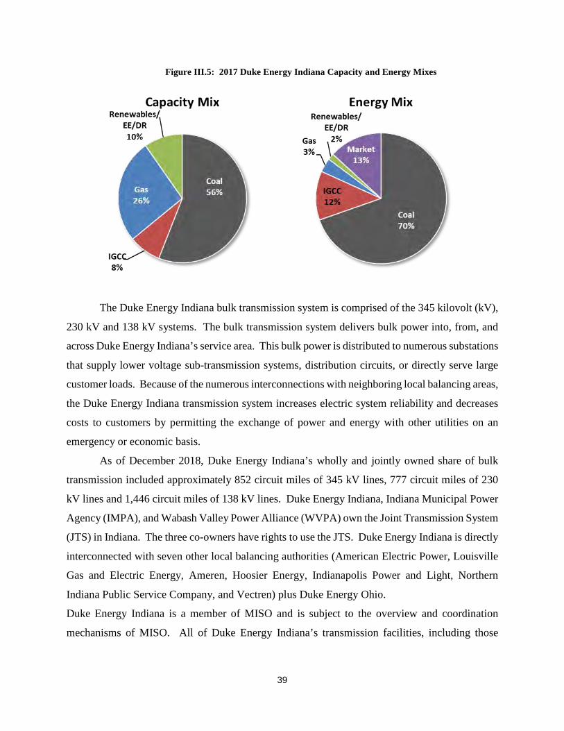
Figure III.5: 2017 Duke Energy Indiana Capacity and Energy Mixes

The Duke Energy Indiana bulk transmission system is comprised of the 345 kilovolt (kV),

230 kV and 138 kV systems. The bulk transmission system delivers bulk power into, from, and

across Duke Energy Indiana’s service area. This bulk power is distributed to numerous substations

that supply lower voltage sub-transmission systems, distribution circuits, or directly serve large

customer loads. Because of the numerous interconnections with neighboring local balancing areas,

the Duke Energy Indiana transmission system increases electric system reliability and decreases

costs to customers by permitting the exchange of power and energy with other utilities on an

emergency or economic basis.

As of December 2018, Duke Energy Indiana’s wholly and jointly owned share of bulk

transmission included approximately 852 circuit miles of 345 kV lines, 777 circuit miles of 230

kV lines and 1,446 circuit miles of 138 kV lines. Duke Energy Indiana, Indiana Municipal Power

Agency (IMPA), and Wabash Valley Power Alliance (WVPA) own the Joint Transmission System

(JTS) in Indiana. The three co-owners have rights to use the JTS. Duke Energy Indiana is directly

interconnected with seven other local balancing authorities (American Electric Power, Louisville

Gas and Electric Energy, Ameren, Hoosier Energy, Indianapolis Power and Light, Northern

Indiana Public Service Company, and Vectren) plus Duke Energy Ohio.

Duke Energy Indiana is a member of MISO and is subject to the overview and coordination

mechanisms of MISO. All of Duke Energy Indiana’s transmission facilities, including those

40

transmission facilities owned by WVPA and IMPA but operated and maintained by Duke Energy

Indiana, are included in these MISO planning processes.

C. CURRENT DEMAND-SIDE PROGRAMS

Duke Energy Indiana has a long history associated with the implementation of EE and DR

programs. Duke Energy Indiana’s EE and DR programs have been offered since 1991 and are

designed to help reduce demand on the Duke Energy Indiana system during times of peak load

and reduce energy consumption during peak and off-peak hours. Demand response programs

include customer-specific contract options and innovative pricing programs.

Implementing cost-effective EE and DR programs helps reduce overall long-term supply

costs. Duke Energy Indiana’s EE and DR programs are primarily selected for implementation

based upon their cost-effectiveness; however, there may be programs, such as a low-income

program, that are chosen for implementation due to desirability from an educational and/or social

perspective.

Current Energy Efficiency Programs

Duke Energy Indiana’s current Energy Efficiency (EE) program portfolio was approved

by the Commission in Cause No. 43955 – DSM4 for the periods 2017-19 and contains the

following set of programs described in greater detail in Appendix D:

Residential Programs

• Smart $aver® Residential HVAC Equipment Attic Insulation and Air Sealing Duct Sealing Heat Pump Water Heater Variable-Speed Pool Pump Referral Programs Free LED Program Specialty Lighting & other energy efficient products Retail Lighting Save Energy and Water Kit Low Income Neighborhood - Neighborhood Energy Saver Program Agency Assistance Portal Low Income Weatherization

41

• Multifamily Energy Efficiency Products & Services • Residential Energy Assessments • My Home Energy Report • Energy Efficiency Education Program for Schools • Power Manager® (Demand Response) • Bring Your Own Thermostat (Demand Response) • Energy Efficient Appliance • Manufactured Home • Multi-Family Retrofit • Residential New Construction

Non-Residential Programs • Smart $aver® Non-Residential Incentive Program Prescriptive Incentives Custom Incentives Performance Incentives

• Small Business Energy Saver • Power Manager® for Business

Current Demand Response Programs

In addition to the Residential Demand Response programs approved in Cause 43955 –

DSM4, Duke Energy Indiana also offers the following Non-Residential Demand Response

programs under its Rider 70 and other special contracts:

• PowerShare® CallOption • Special Curtailment Contracts

42

SECTION IV: DUKE ENERGY INDIANA IN THE FUTURE

Resource planning for an uncertain future requires consideration of the range of operating

conditions the Company may face in both the near and long term. Scenario analysis is a useful tool

for long range planning as it provides a basis for studying the impact of changes in key variables

over time. To achieve this, the scenarios developed must be plausible, internally consistent,

sufficiently different from each other to be meaningful and cover a broad range of potential futures.

The key uncertainties that form the basis of scenarios should be those that are most

impactful to resource selection, have been or are anticipated to be highly variable, and are difficult

to predict with confidence. Through internal analysis and discussions at the first stakeholder

meeting, the key variables selected as the foundation for scenario development were natural gas

prices, carbon regulation, and the cost of renewable technologies. Once the key variables were

determined, base case and alternate forecasts were developed for each and grouped into themes

which align with a narrative describing a future world consistent with the forecasts of the key

variables. To ensure internal consistency of the scenario, additional modeling was conducted to

develop MISO power price projections consistent with the other input variables.

Duke Energy Indiana initially proposed three scenarios; the Reference Case based upon

the corporate base case fundamentals forecasts, the High Tech Future scenario characterized by

increased technological innovation and higher economic growth, and the Slower Innovation

scenario characterized by decreased technological innovation and slower economic growth. After

reviewing these scenarios with stakeholders, two additional scenarios were developed based upon

stakeholder feedback; the Reference Case Scenario without Carbon Legislation, and a Current

Conditions scenario which assumes the status quo or current trends persists in most input variables.

A summary of the five scenarios is shown in the table below followed by more detailed

descriptions throughout the remainder of this section.

43

Table IV.1: Scenario Assumption Summary

A. REFERENCE CASE SCENARIO

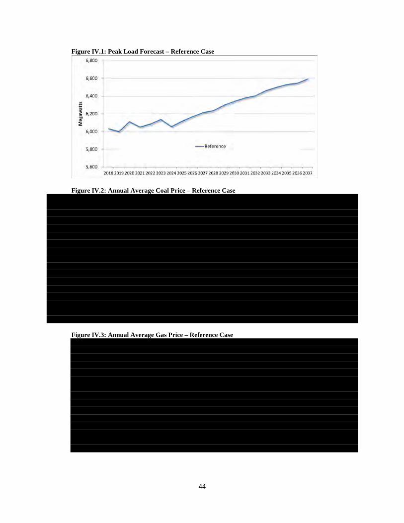
The Reference Case envisions many aspects and trends of the present persisting into the

future. Load growth is moderate with an average annual growth rate of approximately 0.5% over

the 20-year planning period. Technological innovation continues to drive down the cost of

renewable resources and energy efficiency measures, increasing the economic competitiveness

of these resources. Increases in the cost of oil, gas and coal are moderate, based on modest

inflation expectations and incremental improvements in extraction technology and methods.

Public opinion shows support for a response to climate change resulting in the imposition of a

price on carbon emissions of $5/ton beginning in 2025, increasing by $3/ton per year thereafter.

The lower capital costs for renewable projects and presence of a carbon price obviates any push

to extend federal tax incentives for renewables resulting in their phase out in accordance with

current policy.

44

Figure IV.1: Peak Load Forecast – Reference Case

Figure IV.2: Annual Average Coal Price – Reference Case Figure IV.3: Annual Average Gas Price – Reference Case

45

Figure IV.4: Carbon Price – Reference Case

Figure IV.5: Annual Average Power Price – Reference Case Figure IV.6: Installed Utility-Scale Solar Cost (including AFUDC) – Reference Case

46

Figure IV.7: Capacity Factor for new Wind – Reference Case

Figure IV.8: Installed Battery Cost (including AFUDC) – Reference Case

47

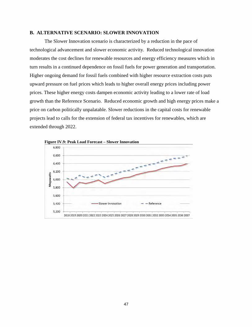
B. ALTERNATIVE SCENARIO: SLOWER INNOVATION

The Slower Innovation scenario is characterized by a reduction in the pace of

technological advancement and slower economic activity. Reduced technological innovation

moderates the cost declines for renewable resources and energy efficiency measures which in

turn results in a continued dependence on fossil fuels for power generation and transportation.

Higher ongoing demand for fossil fuels combined with higher resource extraction costs puts

upward pressure on fuel prices which leads to higher overall energy prices including power

prices. These higher energy costs dampen economic activity leading to a lower rate of load

growth than the Reference Scenario. Reduced economic growth and high energy prices make a

price on carbon politically unpalatable. Slower reductions in the capital costs for renewable

projects lead to calls for the extension of federal tax incentives for renewables, which are

extended through 2022.

Figure IV.9: Peak Load Forecast – Slower Innovation

48

Figure IV.10: Annual Average Coal Price – Slower Innovation Figure IV.11: Annual Average Gas Price – Slower Innovation Figure IV.12: Carbon Price – Slower Innovation

49

Figure IV.13: Annual Average Power Price – Slower Innovation Figure IV.14: Installed Utility-Scale Solar Cost (including AFUDC) – Slower Innovation

50

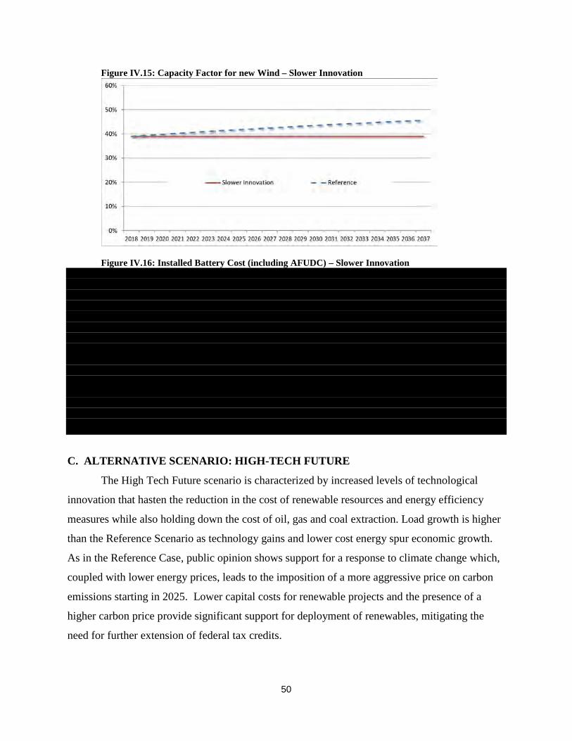
Figure IV.15: Capacity Factor for new Wind – Slower Innovation

Figure IV.16: Installed Battery Cost (including AFUDC) – Slower Innovation

C. ALTERNATIVE SCENARIO: HIGH-TECH FUTURE

The High Tech Future scenario is characterized by increased levels of technological

innovation that hasten the reduction in the cost of renewable resources and energy efficiency

measures while also holding down the cost of oil, gas and coal extraction. Load growth is higher

than the Reference Scenario as technology gains and lower cost energy spur economic growth.

As in the Reference Case, public opinion shows support for a response to climate change which,

coupled with lower energy prices, leads to the imposition of a more aggressive price on carbon

emissions starting in 2025. Lower capital costs for renewable projects and the presence of a

higher carbon price provide significant support for deployment of renewables, mitigating the

need for further extension of federal tax credits.

51

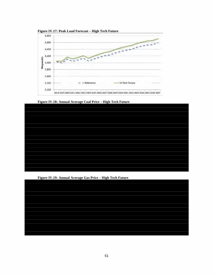
Figure IV.17: Peak Load Forecast – High Tech Future

Figure IV.18: Annual Average Coal Price – High Tech Future Figure IV.19: Annual Average Gas Price – High Tech Future

52

Figure IV.20: Carbon Price – High Tech Future

Figure IV.21: Annual Average Power Price – High Tech Future Figure IV.22: Installed Utility-Scale Solar Cost (including AFUDC) – High Tech Future

53

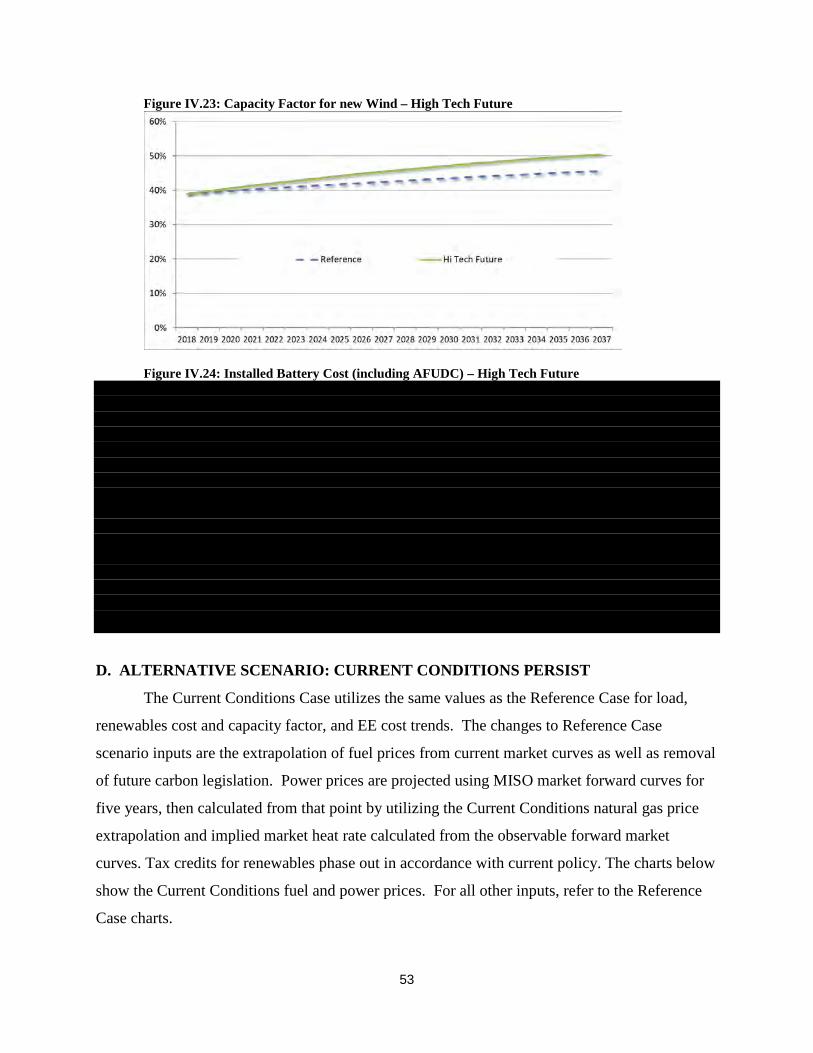
Figure IV.23: Capacity Factor for new Wind – High Tech Future

Figure IV.24: Installed Battery Cost (including AFUDC) – High Tech Future

D. ALTERNATIVE SCENARIO: CURRENT CONDITIONS PERSIST

The Current Conditions Case utilizes the same values as the Reference Case for load,

renewables cost and capacity factor, and EE cost trends. The changes to Reference Case

scenario inputs are the extrapolation of fuel prices from current market curves as well as removal

of future carbon legislation. Power prices are projected using MISO market forward curves for

five years, then calculated from that point by utilizing the Current Conditions natural gas price

extrapolation and implied market heat rate calculated from the observable forward market

curves. Tax credits for renewables phase out in accordance with current policy. The charts below

show the Current Conditions fuel and power prices. For all other inputs, refer to the Reference

Case charts.

54

Figure IV.25: Annual Average Coal Price – Current Conditions Figure IV.26: Annual Average Gas Price – Current Conditions Figure IV.27: Annual Average Power Price – Current Conditions

55

E. REFERENCE CASE WITHOUT CARBON LEGISLATION

The Reference Case without Carbon Legislation scenario utilizes the same values as the

Reference Case for load, fuel, renewables and EE cost trends. The only change to scenario

inputs is the removal of future carbon legislation. This change is further reflected in the modeled

MISO power prices. This scenario clearly demonstrates the impact of the presence or absence of

a price on carbon emissions, assuming all other inputs remain fixed. The chart below shows the

difference in MISO power prices resulting from the removal of the carbon price. For all other

inputs, refer to the Reference Case charts. Tax credits for renewables phase out in accordance

with current policy.

Figure IV.28: Annual Average Power Price – Reference Case without Carbon Legislation

56

SECTION V: CANDIDATE RESOURCE PORTFOLIOS

This section includes descriptions and analysis of the resource portfolios we evaluated for

the 2018 IRP. These include the optimized portfolios, each of which is designed to minimize costs

under a particular scenario, and the alternative portfolios, which are designed to improve upon the

optimized portfolios and balance our objectives in ways that SO cannot. The first part of this

section is a detailed list of the resource types available for selection in the IRP.

A. OBJECTIVES OF THE 2018 IRP

The major objectives of the IRP presented in this filing, developed with input from Duke

Energy Indiana stakeholders, are:

• Provide adequate, reliable, efficient, economic service. The metric for this objective is

PVRR.

• Maintain the flexibility and ability to alter the plan in the future as circumstances change.

All else being equal, portfolios that include more, larger, singular resource decisions are

less flexible.

• Minimize environmental impact, including carbon emissions. Because carbon emissions

are highly correlated with other environmental impacts, the metric for this objective is

annual CO2 emissions.

• Minimize risk. The most pressing risk factors for this IRP, as determined in consultation

with stakeholders, are reliability risk, compliance and cost risk associated with potential

carbon legislation, and cost risk associated with over-reliance on net energy purchases from

the MISO market. Reliability is addressed via the inclusion of the planning reserve margin

requirement in portfolio development, carbon risk is addressed by the inclusion of a carbon

price in two of the scenarios for this IRP, and the metric for market risk is the portion of

total annual energy demand that is met with market purchases.

57

B. CANDIDATE RESOURCES FOR THE 2018 IRP

Supply-Side Resources

Based on the technical and commercial availability screening described in Section II.C, the

following technologies were excluded from consideration in this IRP: small modular nuclear

reactors, solar steam augmentation, fuel cells, supercritical CO2 Brayton cycle, and liquid air

energy storage, geothermal, offshore wind, landfill gas, pumped storage hydropower, and

compressed air energy storage.

The Company considered for inclusion in this IRP a diverse range of technologies utilizing

a variety of different fuels, including pulverized coal units, CTs, CCs, combined heat and power,

reciprocating engines, and nuclear stations. In addition, onshore wind, solar photovoltaic, and

battery storage options were included in the analysis. Table V.1 below provides an overview of

the characteristics of the supply-side resources available for selection in this IRP. Further detail

can be found in Appendix C.

58

Table V.1: Unit Characteristics for Potential Supply-Side Resource Additions In addition to the characteristics listed in the table above, we imposed certain constraints on the

model governing when certain resources could be added or retired and how much of each

resource could be constructed in each year. The following limitations were imposed:

• No unit was permitted to retire before 2024. This reflects the time it would take for the

company to prepare to take a unit offline (including any regulatory filings and design,

permitting, and construction of replacement resources), as well as make any required

transmission upgrades. The exception is the retirement of Gallagher Units 2&4 in

December 2022, to which we are already committed, and for which we have already

conducted the necessary up-front preparations. The Gallagher retirement is part of all

portfolios considered for the IRP. In addition, Edwardsport IGCC was not considered for

59

retirement in this IRP. The plant is the newest on our system and has the longest

estimated life (2045), well past the review period in this IRP. The plant has successfully

improved operations over the past several years and going forward will be focused on

reducing its ongoing maintenance costs. A diversified portfolio will continue to be a

priority with Edwardsport IGCC contributing to the fleet’s diversity over the planning

period.

• Retirement analysis was conducted only on the coal units. Other units were not

considered for economic retirement.

• The SO model is permitted to add fractions of nuclear, coal, CC and CT units to allow us

to better understand how the timing of resource needs is distributed and to reflect our

ability to partner with other entities on new generating stations.

• Annual capacity additions for each resource type are capped to reflect practical

constraints. The caps are: 2,120 MW of ultra-supercritical coal, 2,070 MW of IGCC, 840

MW of nuclear, 3,100 MW of CC, 3,225 MW of CT, 80 MW of CHP, 1,212 MW of

reciprocating engines, 2,500 MW of solar, 250 MW of wind, and 250 MW of batteries.

• The time required to permit and construct each unit type is reflected in the first year

available shown in Table V.1.

• A variable operating cost of $5/MWh is imposed on solar additions over 800 MW of

nameplate capacity. This reflects our estimate of the additional cost of operating the

system with a high penetration of solar resource. The cost is increased by $5/MWh for

each additional 800 MW tranche of solar.

• Solar and wind resources contribute to meeting the planning reserve margin requirement

at less than nameplate capacity, reflecting the fact that these resources may not be fully

available at the time of peak load. Solar is counted at 50% of nameplate capacity (0% in

winter) and wind at 13%, which is consistent with MISO’s treatment of these resource

types. Battery storage is valued at 80% of installed capacity to reflect the possibility that

the battery may not be fully charged at the peak hour.

60

Demand-Side Resources

For the purposes of the 2018 IRP, the Company developed 150 sub-portfolios of EE programs

(also referred to as “bundles”). These bundles were designed to be treated as demand-side

resource options for selection by the IRP process and EE measures were grouped together in

these bundles based on the hourly shape of the savings contributed by these measures. For each

of these hourly shapes, three different levels of customer participation, a Base Case, a High Case,

and an Extra-High Case, were created. In order to reduce the amount of time required for

analyzing the overall portfolio of bundles, the Company further consolidated the 150 bundles

into a final group of 70 bundles. The consolidation was done by combining together the Base,

High and Extra-High cases for certain bundles of hourly shapes where the incremental amounts

of the High and Extra-High cases were not large compared to the Base Case. These bundles

were available for selection in the SO model alongside the supply-side resource options.

Additional details on demand-side resources, bundles and the screening process for demand-side

resources are available in Appendix D.

Resource Decisions Common to All Portfolios

Certain resource decisions to which the Company had committed prior to the completion of this

IRP analysis are included in all portfolios. These are:

• Retirement of Gallagher Units 2&4 in December 2022

• EE programs through 2020 as approved under Cause No. 43955 DSM-4

• 16 MW CHP project with planned completion in 2021

• 6 MW of solar added in 2019 and 2 MW in 2020

• 10 MW of battery storage added in 2019 and 5 MW added in 2020

• 100 MW Benton County wind PPA expires in 2028

• 21 MW of solar PPAs expire in 2036

• Contracted purchase of 8 MW of CT capacity ends in 2019

• Contracted sale of 50 MW of CT capacity at Henry County ends in 2022

• Demand response is not selected by the model. DR additions are forecasted and the

forecast is consistent across all portfolios

61

C. OPTIMIZED RESOURCE PORTFOLIOS

Recall that an optimized portfolio is designed to be least cost under the assumptions of a

specific scenario. Those scenario assumptions are the inputs to the SO model, which selects

resource additions and retirements to minimize the PVRR for the portfolio while meeting the

planning reserve margin requirement. There are five optimized portfolios, one for each IRP

scenario.

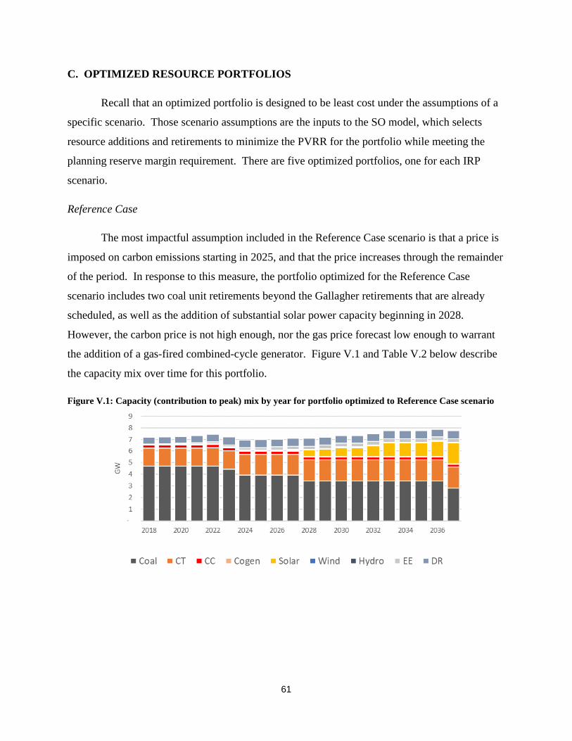
Reference Case

The most impactful assumption included in the Reference Case scenario is that a price is

imposed on carbon emissions starting in 2025, and that the price increases through the remainder

of the period. In response to this measure, the portfolio optimized for the Reference Case

scenario includes two coal unit retirements beyond the Gallagher retirements that are already

scheduled, as well as the addition of substantial solar power capacity beginning in 2028.

However, the carbon price is not high enough, nor the gas price forecast low enough to warrant

the addition of a gas-fired combined-cycle generator. Figure V.1 and Table V.2 below describe

the capacity mix over time for this portfolio.

Figure V.1: Capacity (contribution to peak) mix by year for portfolio optimized to Reference Case scenario

62

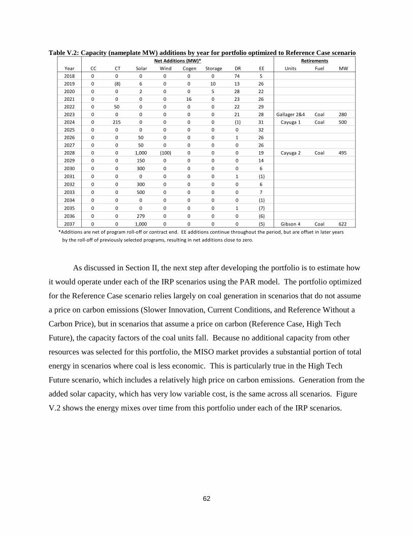
Table V.2: Capacity (nameplate MW) additions by year for portfolio optimized to Reference Case scenario

As discussed in Section II, the next step after developing the portfolio is to estimate how

it would operate under each of the IRP scenarios using the PAR model. The portfolio optimized

for the Reference Case scenario relies largely on coal generation in scenarios that do not assume

a price on carbon emissions (Slower Innovation, Current Conditions, and Reference Without a

Carbon Price), but in scenarios that assume a price on carbon (Reference Case, High Tech

Future), the capacity factors of the coal units fall. Because no additional capacity from other

resources was selected for this portfolio, the MISO market provides a substantial portion of total

energy in scenarios where coal is less economic. This is particularly true in the High Tech

Future scenario, which includes a relatively high price on carbon emissions. Generation from the

added solar capacity, which has very low variable cost, is the same across all scenarios. Figure

V.2 shows the energy mixes over time from this portfolio under each of the IRP scenarios.

Year CC CT Solar Wind Cogen Storage DR EE Units Fuel MW2018 0 0 0 0 0 0 74 52019 0 (8) 6 0 0 10 13 262020 0 0 2 0 0 5 28 222021 0 0 0 0 16 0 23 262022 0 50 0 0 0 0 22 292023 0 0 0 0 0 0 21 28 Gallager 2&4 Coal 2802024 0 215 0 0 0 0 (1) 31 Cayuga 1 Coal 5002025 0 0 0 0 0 0 0 322026 0 0 50 0 0 0 1 262027 0 0 50 0 0 0 0 262028 0 0 1,000 (100) 0 0 0 19 Cayuga 2 Coal 4952029 0 0 150 0 0 0 0 142030 0 0 300 0 0 0 0 62031 0 0 0 0 0 0 1 (1)2032 0 0 300 0 0 0 0 62033 0 0 500 0 0 0 0 72034 0 0 0 0 0 0 0 (1)2035 0 0 0 0 0 0 1 (7)2036 0 0 279 0 0 0 0 (6)2037 0 0 1,000 0 0 0 0 (5) Gibson 4 Coal 622

*Additions are net of program roll-off or contract end. EE additions continue throughout the period, but are offset in later years by the roll-off of previously selected programs, resulting in net additions close to zero.

RetirementsNet Additions (MW)*

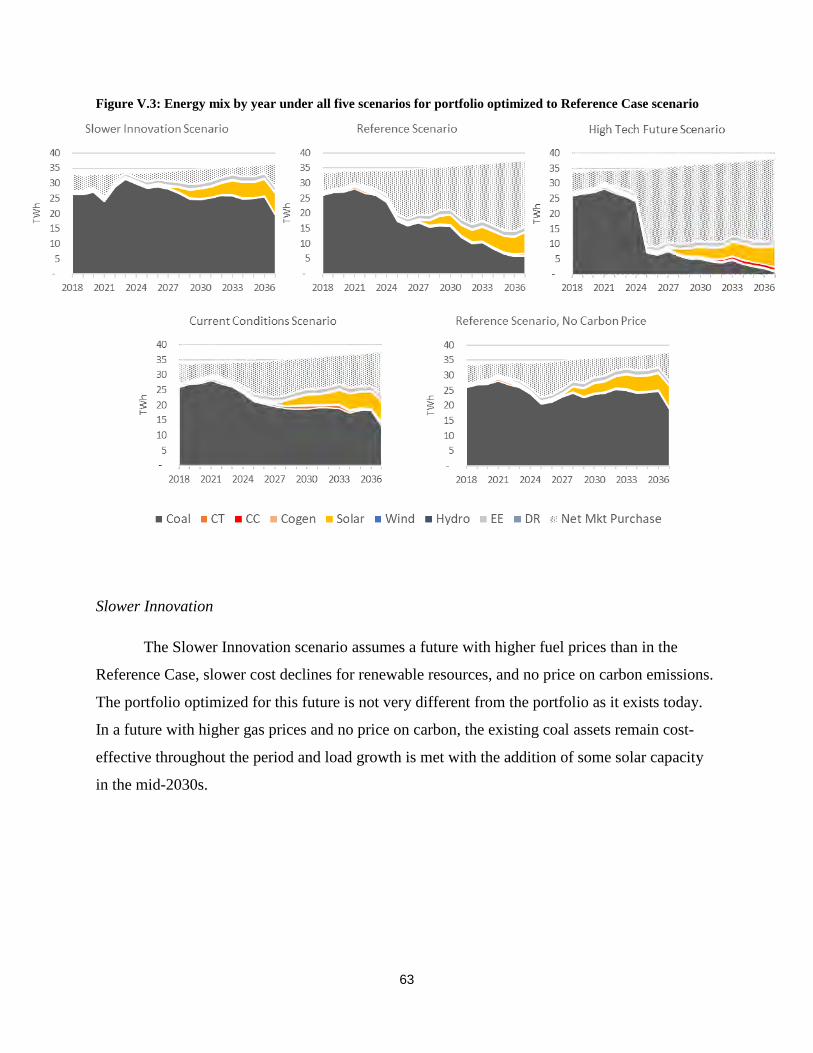
63

Figure V.3: Energy mix by year under all five scenarios for portfolio optimized to Reference Case scenario

Slower Innovation

The Slower Innovation scenario assumes a future with higher fuel prices than in the

Reference Case, slower cost declines for renewable resources, and no price on carbon emissions.

The portfolio optimized for this future is not very different from the portfolio as it exists today.

In a future with higher gas prices and no price on carbon, the existing coal assets remain cost-

effective throughout the period and load growth is met with the addition of some solar capacity

in the mid-2030s.

64

Figure V.4: Capacity (contribution to peak) mix by year for portfolio optimized to Slower Innovation scenario

Table V.3: Capacity (nameplate MW) additions by year for portfolio optimized to Slower Innovation scenario

The portfolio optimized for the Slower Innovation scenario remains weighted towards

coal-fired generating capacity throughout the planning period. In scenarios that have no price on

carbon emissions, coal-fired generation supplies over half of total energy in all years. However,

coal capacity factors do decline in the Current Conditions scenario as lower gas prices challenge

the competitiveness of coal in many hours and there is a gradual shift toward purchasing lower

cost energy from the MISO market. In the scenarios that include a price on carbon, the coal-

Year CC CT Solar Wind Cogen Storage DR EE Units Fuel MW2018 0 0 0 0 0 0 74 52019 0 (8) 6 0 0 10 13 262020 0 0 2 0 0 5 28 222021 0 0 0 0 16 0 23 232022 0 50 0 0 0 0 22 222023 0 0 0 0 0 0 21 22 Gallager 2&4 Coal 2802024 0 0 0 0 0 0 (1) 232025 0 0 0 0 0 0 0 212026 0 0 0 0 0 0 1 192027 0 0 0 0 0 0 0 202028 0 0 0 (100) 0 0 0 172029 0 0 0 0 0 0 0 122030 0 0 0 0 0 0 0 52031 0 0 0 0 0 0 1 12032 0 0 0 0 0 0 0 42033 0 0 0 0 0 0 0 52034 0 0 0 0 0 0 0 (1)2035 0 0 0 0 0 0 1 (6)2036 0 0 279 0 0 0 0 (7)2037 0 0 500 0 0 0 0 (1)

*Additions are net of program roll-off or contract end. EE additions continue throughout the period, but are offset in later years by the roll-off of previously selected programs, resulting in net additions close to zero.

RetirementsNet Additions (MW)*

65

heavy fleet is much less competitive and the shift towards energy supplied by the market is more

dramatic. Note that in the High Tech Future scenario, which includes both a relatively high price

on carbon emissions and a lower forecast for gas prices, coal is almost driven out of the energy

mix entirely with the market making up the difference.

Figure V.5: Energy mix by year under all five scenarios for portfolio optimized to Slower Innovation scenario

High Tech Future

The High Tech Future scenario describes a world with lower gas prices than in the

Reference Case, more rapidly declining costs for renewable resources, and a higher price on

carbon emissions. The portfolio optimized for this scenario includes the retirement of all

conventional coal-fired generation by the early 2030s and the replacement of that capacity with a

combination of gas-fired combined-cycle units and solar power.

66

Figure V.6: Capacity (contribution to peak) mix by year for portfolio optimized to High Tech Future scenario

Table V.4: Capacity (nameplate MW) additions by year for portfolio optimized to High Tech Future scenario

The combined-cycle generation added to the portfolio optimized for the High Tech

Future scenario is competitive in scenarios where coal is not, helping to limit market exposure.

In Slower Innovation and Reference Scenario, No Carbon Price, which feature higher gas prices

than the High Tech Future and no price on carbon emissions, the portfolio optimized for the

High Tech Future scenario leans more heavily on energy purchased from the market than do

Year CC CT Solar Wind Cogen Storage DR EE Units Fuel MW2018 0 0 0 0 0 0 74 52019 0 (8) 6 0 0 10 13 262020 0 0 2 0 0 5 28 222021 0 0 0 0 16 0 23 302022 0 50 0 0 0 0 22 372023 0 0 0 0 0 0 21 35 Gallager 2&4 Coal 2802024 310 0 0 0 0 0 (1) 39 Gibson 3 Coal 6302025 0 0 0 0 0 0 0 372026 620 0 0 0 0 0 1 30 Gibson 5 Coal 3102027 310 0 300 0 0 0 0 27 Cayuga 1 Coal 5002028 0 0 1,100 (100) 0 0 0 21 Gibson 2 Coal 6302029 0 0 300 0 0 0 0 142030 0 0 0 0 0 0 0 52031 620 0 200 0 0 0 1 (4) Cayuga 2 Coal 4952032 620 0 500 0 0 0 0 4 Gibson 1 Coal 6302033 620 0 0 0 0 0 0 6 Gibson 4 Coal 6222034 0 0 0 0 0 0 0 (2)2035 0 0 0 0 0 0 1 (8)2036 0 0 279 0 0 0 0 (6)2037 0 0 500 0 0 0 0 (6)

*Additions are net of program roll-off or contract end. EE additions continue throughout the period, but are offset in later years by the roll-off of previously selected programs, resulting in net additions close to zero.

RetirementsNet Additions (MW)*

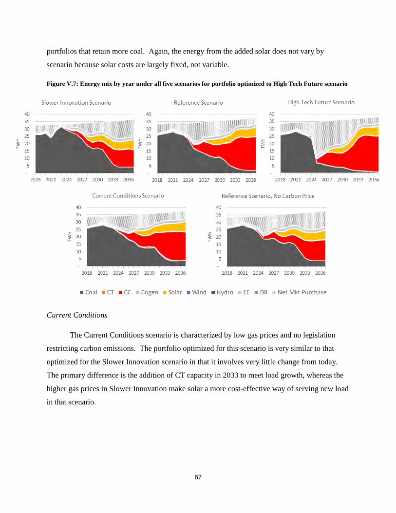
67

portfolios that retain more coal. Again, the energy from the added solar does not vary by

scenario because solar costs are largely fixed, not variable.

Figure V.7: Energy mix by year under all five scenarios for portfolio optimized to High Tech Future scenario

Current Conditions

The Current Conditions scenario is characterized by low gas prices and no legislation

restricting carbon emissions. The portfolio optimized for this scenario is very similar to that

optimized for the Slower Innovation scenario in that it involves very little change from today.

The primary difference is the addition of CT capacity in 2033 to meet load growth, whereas the

higher gas prices in Slower Innovation make solar a more cost-effective way of serving new load

in that scenario.

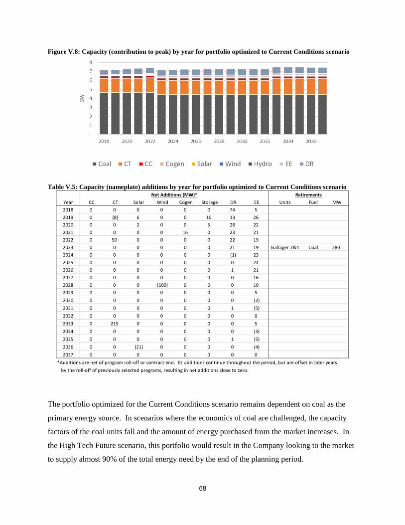
68

Figure V.8: Capacity (contribution to peak) by year for portfolio optimized to Current Conditions scenario

Table V.5: Capacity (nameplate) additions by year for portfolio optimized to Current Conditions scenario

The portfolio optimized for the Current Conditions scenario remains dependent on coal as the

primary energy source. In scenarios where the economics of coal are challenged, the capacity

factors of the coal units fall and the amount of energy purchased from the market increases. In

the High Tech Future scenario, this portfolio would result in the Company looking to the market

to supply almost 90% of the total energy need by the end of the planning period.

Year CC CT Solar Wind Cogen Storage DR EE Units Fuel MW2018 0 0 0 0 0 0 74 52019 0 (8) 6 0 0 10 13 262020 0 0 2 0 0 5 28 222021 0 0 0 0 16 0 23 212022 0 50 0 0 0 0 22 192023 0 0 0 0 0 0 21 19 Gallager 2&4 Coal 2802024 0 0 0 0 0 0 (1) 232025 0 0 0 0 0 0 0 242026 0 0 0 0 0 0 1 212027 0 0 0 0 0 0 0 162028 0 0 0 (100) 0 0 0 102029 0 0 0 0 0 0 0 52030 0 0 0 0 0 0 0 (2)2031 0 0 0 0 0 0 1 (5)2032 0 0 0 0 0 0 0 02033 0 215 0 0 0 0 0 52034 0 0 0 0 0 0 0 (3)2035 0 0 0 0 0 0 1 (5)2036 0 0 (21) 0 0 0 0 (4)2037 0 0 0 0 0 0 0 0

*Additions are net of program roll-off or contract end. EE additions continue throughout the period, but are offset in later years by the roll-off of previously selected programs, resulting in net additions close to zero.

RetirementsNet Additions (MW)*

69

Figure V.9: Energy mix under all five scenarios for portfolio optimized to Current Conditions scenario

Reference Case Without Carbon Legislation

Legislative action imposing a price on carbon emissions is one of the most impactful

assumptions we consider in this IRP. For this reason, we created a portfolio optimized for a

scenario identical to our Reference Case scenario in all respects except for the carbon price. The

portfolio optimized for the Reference Case Without Carbon Legislation is very similar to the

portfolio optimized for the Slower Innovation scenario, with few changes until the end of the

planning period when some solar capacity is added to serve new load. One significant difference

is the retirement of Cayuga 2 in 2037, the final year of the planning period. Recall that gas

prices are lower in the Reference Case Without Carbon Legislation than they are in Slower

Innovation.

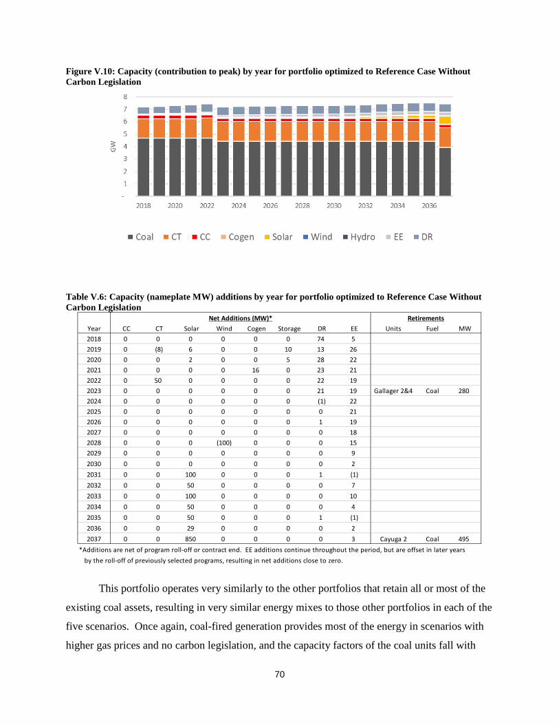
70

Figure V.10: Capacity (contribution to peak) by year for portfolio optimized to Reference Case Without Carbon Legislation

Table V.6: Capacity (nameplate MW) additions by year for portfolio optimized to Reference Case Without Carbon Legislation

This portfolio operates very similarly to the other portfolios that retain all or most of the

existing coal assets, resulting in very similar energy mixes to those other portfolios in each of the

five scenarios. Once again, coal-fired generation provides most of the energy in scenarios with

higher gas prices and no carbon legislation, and the capacity factors of the coal units fall with

Year CC CT Solar Wind Cogen Storage DR EE Units Fuel MW2018 0 0 0 0 0 0 74 52019 0 (8) 6 0 0 10 13 262020 0 0 2 0 0 5 28 222021 0 0 0 0 16 0 23 212022 0 50 0 0 0 0 22 192023 0 0 0 0 0 0 21 19 Gallager 2&4 Coal 2802024 0 0 0 0 0 0 (1) 222025 0 0 0 0 0 0 0 212026 0 0 0 0 0 0 1 192027 0 0 0 0 0 0 0 182028 0 0 0 (100) 0 0 0 152029 0 0 0 0 0 0 0 92030 0 0 0 0 0 0 0 22031 0 0 100 0 0 0 1 (1)2032 0 0 50 0 0 0 0 72033 0 0 100 0 0 0 0 102034 0 0 50 0 0 0 0 42035 0 0 50 0 0 0 1 (1)2036 0 0 29 0 0 0 0 22037 0 0 850 0 0 0 0 3 Cayuga 2 Coal 495

*Additions are net of program roll-off or contract end. EE additions continue throughout the period, but are offset in later years by the roll-off of previously selected programs, resulting in net additions close to zero.

RetirementsNet Additions (MW)*

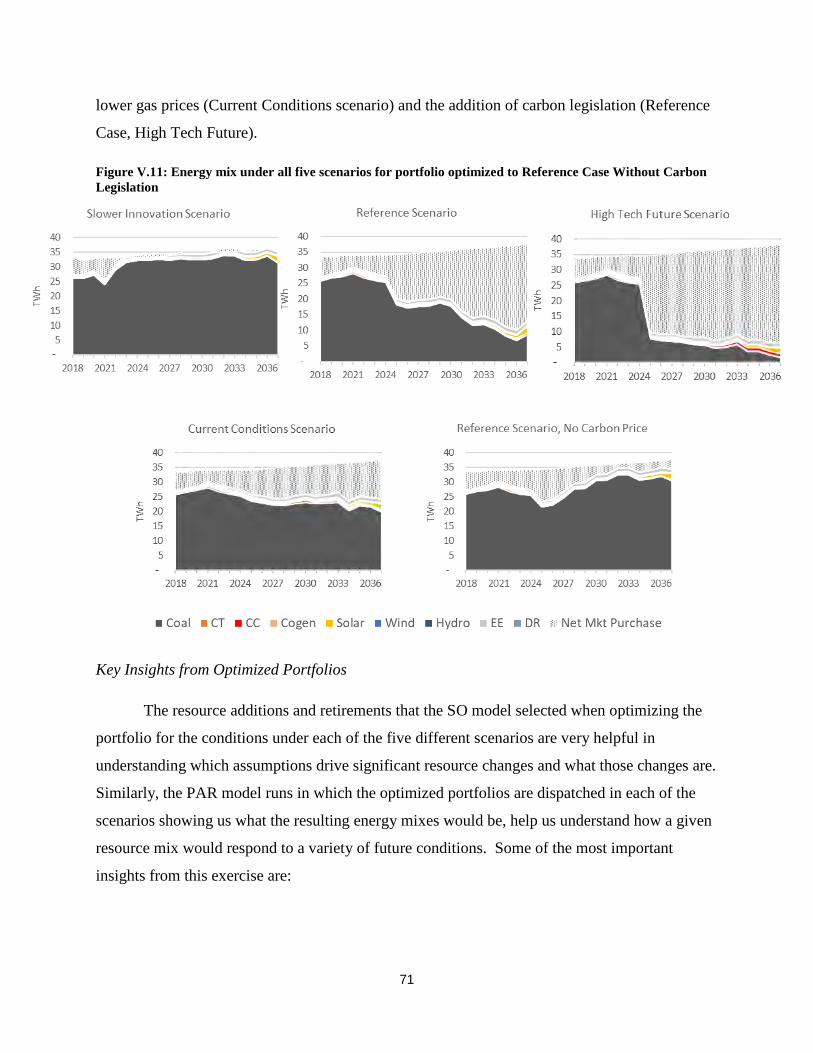
71

lower gas prices (Current Conditions scenario) and the addition of carbon legislation (Reference

Case, High Tech Future).

Figure V.11: Energy mix under all five scenarios for portfolio optimized to Reference Case Without Carbon Legislation

Key Insights from Optimized Portfolios

The resource additions and retirements that the SO model selected when optimizing the

portfolio for the conditions under each of the five different scenarios are very helpful in

understanding which assumptions drive significant resource changes and what those changes are.

Similarly, the PAR model runs in which the optimized portfolios are dispatched in each of the

scenarios showing us what the resulting energy mixes would be, help us understand how a given

resource mix would respond to a variety of future conditions. Some of the most important

insights from this exercise are:

72

• In a future without carbon legislation, the least cost portfolio is one that retains the

existing coal assets for capacity purposes and adds little new capacity. This is true even

in a future with very low gas prices, as in the Current Conditions scenario.

• A price on carbon emissions would accelerate coal retirements, resulting in a shift

towards CCs, CTs, and solar.

• Gas and solar are consistently selected over wind, which has a low capacity value (13%

of nameplate) and tends to generate more energy at times when demand is low.

• If the portfolio remained weighted towards coal, the Company would rely heavily on the

MISO market for low cost energy if a price were imposed on carbon emissions. With a

more diverse portfolio, the Company would be more self-reliant across a broader range of

conditions.

D. SENSITIVITY ANALYSIS

As discussed in Chapter 2, sensitivity analysis is an important tool for assessing how

changes to individual assumptions could impact our resource selections. If a change to a

particular assumption results in a significant change to the portfolio, then we know that it is very

important to either forecast that variable correctly or, more reasonably, to maintain flexibility

and be ready to respond to different outcomes for that variable. Reviewing the similarities and

differences across the optimized portfolios helps us understand which inputs warrant further

examination via sensitivity analysis.

Fuel Prices

The economic competitiveness of our coal assets is heavily influenced by the price of

coal relative to the price of natural gas. The price of coal is a major driver of our cost of

generation, and the price of gas is a major driver of price of energy in the MISO market. The

relative economics of coal generation are an important factor in retirement analysis, so it is

necessary for us to analyze both high gas prices relative to coal and low gas prices relative to

coal. We expect coal prices to be very stable throughout the planning period, so we focus on gas

prices, which are much more volatile, for this analysis. Because coal prices are stable, our

Slower Innovation scenario is essentially a “high gas” case. Similarly, our Current Conditions

73

scenario is a “low gas” case. The other assumptions are similar enough between those two

scenarios for us to be confident that comparing the respective optimized portfolios can tell us

whether we need to explore the question of fuel prices further. Since the two optimized

portfolios are nearly identical, we conclude that fuel prices alone will not be a major driver of

coal retirements. No additional sensitivity analysis is required.

Load

The top priority for the IRP is to design a resource portfolio that will reliably serve load

throughout the planning period. That makes the load forecast a very important input to the

process. If our load forecast is too low then reliability may be impacted, but if the forecast is too

high then we may build more capacity than necessary, adding unnecessary cost. The former risk

is mitigated by the inclusion of the planning reserve margin by which we retain capacity slightly

in excess of what we expect to need. In addition, some resources, like combustion turbines and

solar plants, can be added relatively quickly and in relatively small increments. For these

reasons, we conclude that the high load forecast included in the High Tech Future scenario

adequately addresses the possibility of actual load growth being more rapid than what is

anticipated in our Reference Case forecast.

Similarly, our analysis of optimized portfolios indicates that major new capacity

additions will be driven largely by coal retirements rather than by load growth. Therefore, we

expect that the risk of over-building capacity is relatively low. However, because capacity

additions cannot be undone, the decision to build carries more risk than the decision to wait. For

this reason, we conducted an additional “flat load” sensitivity analysis to assess how our

portfolio decisions might be impacted by load growth below even our “low load” forecast.

For this analysis, we re-ran the SO model under the Reference Case and High Tech

Future scenarios assuming load remains fixed at current levels (flat load) over the entire planning

period (no other assumptions were changed). We selected the High Tech Future in addition to

the Reference Case because that is the scenario with the highest load forecast, so we would

expect that the flat load assumption would be most impactful on the optimized portfolio for the

High Tech Future. The differences between the original optimized portfolios for those scenarios

and the new optimized portfolios that result from the flat load assumption provide insight into

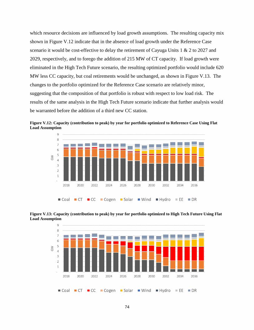
74

which resource decisions are influenced by load growth assumptions. The resulting capacity mix

shown in Figure V.12 indicate that in the absence of load growth under the Reference Case

scenario it would be cost-effective to delay the retirement of Cayuga Units 1 & 2 to 2027 and

2029, respectively, and to forego the addition of 215 MW of CT capacity. If load growth were

eliminated in the High Tech Future scenario, the resulting optimized portfolio would include 620

MW less CC capacity, but coal retirements would be unchanged, as shown in Figure V.13. The

changes to the portfolio optimized for the Reference Case scenario are relatively minor,

suggesting that the composition of that portfolio is robust with respect to low load risk. The

results of the same analysis in the High Tech Future scenario indicate that further analysis would

be warranted before the addition of a third new CC station.

Figure V.12: Capacity (contribution to peak) by year for portfolio optimized to Reference Case Using Flat Load Assumption

Figure V.13: Capacity (contribution to peak) by year for portfolio optimized to High Tech Future Using Flat Load Assumption

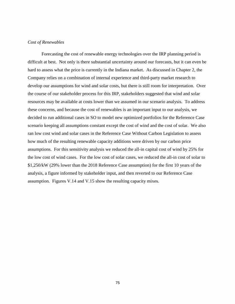
75

Cost of Renewables

Forecasting the cost of renewable energy technologies over the IRP planning period is

difficult at best. Not only is there substantial uncertainty around our forecasts, but it can even be

hard to assess what the price is currently in the Indiana market. As discussed in Chapter 2, the

Company relies on a combination of internal experience and third-party market research to

develop our assumptions for wind and solar costs, but there is still room for interpretation. Over

the course of our stakeholder process for this IRP, stakeholders suggested that wind and solar

resources may be available at costs lower than we assumed in our scenario analysis. To address

these concerns, and because the cost of renewables is an important input to our analysis, we

decided to run additional cases in SO to model new optimized portfolios for the Reference Case

scenario keeping all assumptions constant except the cost of wind and the cost of solar. We also

ran low cost wind and solar cases in the Reference Case Without Carbon Legislation to assess

how much of the resulting renewable capacity additions were driven by our carbon price

assumptions. For this sensitivity analysis we reduced the all-in capital cost of wind by 25% for

the low cost of wind cases. For the low cost of solar cases, we reduced the all-in cost of solar to

$1,250/kW (29% lower than the 2018 Reference Case assumption) for the first 10 years of the

analysis, a figure informed by stakeholder input, and then reverted to our Reference Case

assumption. Figures V.14 and V.15 show the resulting capacity mixes.

76

Figure V.14: Capacity (contribution to peak) by year for portfolio optimized for low cost of wind in Reference Case and Reference Case Without Carbon Legislation scenarios

77

Figure V.15: Capacity (contribution to peak) by year for portfolio optimized for low cost of solar in Reference Case and Reference Case Without Carbon Legislation scenarios

Notice that the new portfolios optimized for the Reference Case Without Carbon

Legislation do not include any additional renewable capacity, wind or solar, until the second half

of the planning period. This suggests that without a price on carbon, it is not cost-effective to

add renewable capacity to the system, even at capital costs well below our Reference Case

assumptions, for at least a decade. However, if we could be certain that carbon legislation would

pass and when, of which the model has perfect foresight in this scenario, then it would make

sense to start adding solar capacity in the relatively near term if it could be secured at very low

cost. Given the state of carbon policy, we do not have the certainty to justify such large scale

immediate action.

78

E. ALTERNATIVE PORTFOLIOS

Developing optimized portfolios helped us understand how the resource mix should be

adjusted to adapt to changes in key variables like load, fuel prices, and carbon legislation.

Running those portfolios through the PAR model showed us given resource mixes would operate

under different future conditions. Our sensitivity analysis provided additional insight to how the

resource mix might be adjusted if load were below even our low forecast, and how the Company

might (or might not) be able to take advantage of lower-than-expected renewable energy costs in

the absence of a near-term capacity need. All of this provides a starting point for developing

alternative portfolios designed to retain the strengths of the optimized portfolios while

minimizing risks. We identified the following as areas of focus for alternative portfolios:

• There are dramatic differences between portfolios optimized for a future with

carbon legislation and those optimized for a future without. Given the

unpredictability of this issue, we need a plan that prepares us for a low carbon

future without incurring major costs prematurely.

• Several of our optimized portfolios would rely heavily on market energy under

certain scenarios. The SO model selects resources as if our market price forecasts

are 100% accurate, but we could be exposed to considerable cost risk if prices

exceed our expectations. We need a plan that limits market exposure while still

allowing us to capture some of the potential benefits of low market prices.

• The SO model does not account for feedbacks by which resource choices may

change the trajectory of certain inputs. This is particularly true in the case of

renewables, where extensive adoption of solar capacity could dramatically affect

daytime power prices. We need a plan that accounts for the fact that the relative

value of wind may increase in the future.

• Unit retirements selected by the SO model are based entirely on as modeled cost

and capacity need. The model does not account for other practical constraints

such as known differences in condition among similar units, joint ownership, site

costs shared with other units, transmission constraints, etc. We need a plan that is

operable in the real world.

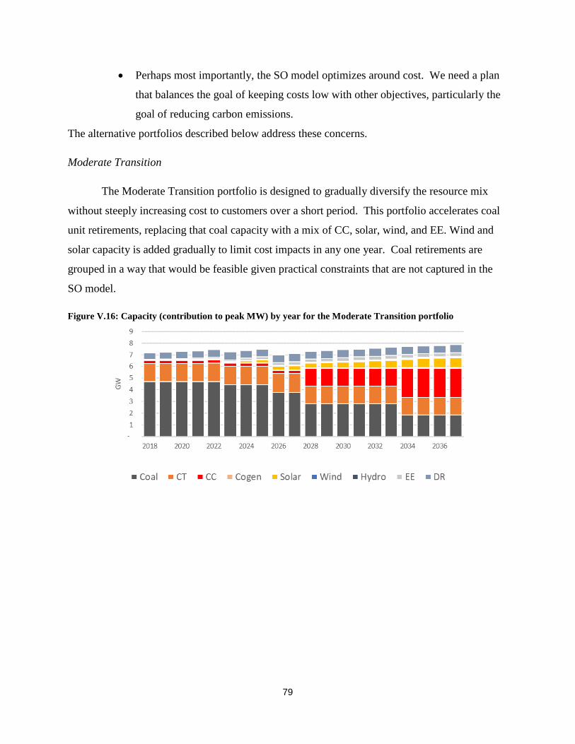
79

• Perhaps most importantly, the SO model optimizes around cost. We need a plan

that balances the goal of keeping costs low with other objectives, particularly the

goal of reducing carbon emissions.

The alternative portfolios described below address these concerns.

Moderate Transition

The Moderate Transition portfolio is designed to gradually diversify the resource mix

without steeply increasing cost to customers over a short period. This portfolio accelerates coal

unit retirements, replacing that coal capacity with a mix of CC, solar, wind, and EE. Wind and

solar capacity is added gradually to limit cost impacts in any one year. Coal retirements are

grouped in a way that would be feasible given practical constraints that are not captured in the

SO model.

Figure V.16: Capacity (contribution to peak MW) by year for the Moderate Transition portfolio

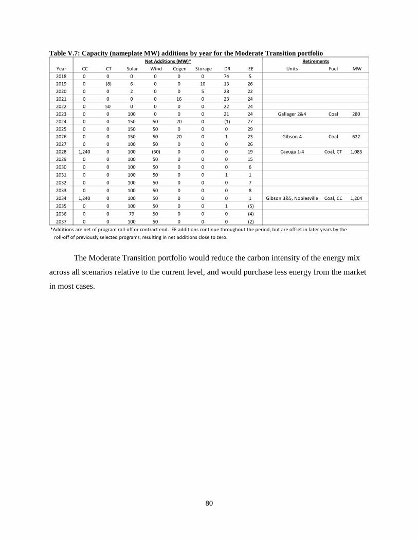
80

Table V.7: Capacity (nameplate MW) additions by year for the Moderate Transition portfolio

The Moderate Transition portfolio would reduce the carbon intensity of the energy mix

across all scenarios relative to the current level, and would purchase less energy from the market

in most cases.

Year CC CT Solar Wind Cogen Storage DR EE Units Fuel MW2018 0 0 0 0 0 0 74 52019 0 (8) 6 0 0 10 13 262020 0 0 2 0 0 5 28 222021 0 0 0 0 16 0 23 242022 0 50 0 0 0 0 22 242023 0 0 100 0 0 0 21 24 Gallager 2&4 Coal 2802024 0 0 150 50 20 0 (1) 272025 0 0 150 50 0 0 0 292026 0 0 150 50 20 0 1 23 Gibson 4 Coal 6222027 0 0 100 50 0 0 0 262028 1,240 0 100 (50) 0 0 0 19 Cayuga 1-4 Coal, CT 1,0852029 0 0 100 50 0 0 0 152030 0 0 100 50 0 0 0 62031 0 0 100 50 0 0 1 12032 0 0 100 50 0 0 0 72033 0 0 100 50 0 0 0 82034 1,240 0 100 50 0 0 0 1 Gibson 3&5, Noblesville Coal, CC 1,2042035 0 0 100 50 0 0 1 (5)2036 0 0 79 50 0 0 0 (4)2037 0 0 100 50 0 0 0 (2)

*Additions are net of program roll-off or contract end. EE additions continue throughout the period, but are offset in later years by the roll-off of previously selected programs, resulting in net additions close to zero.

RetirementsNet Additions (MW)*

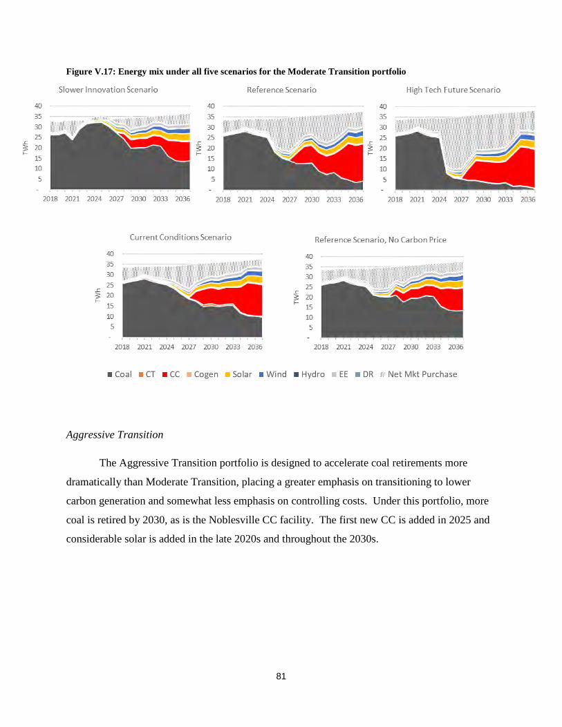
81

Figure V.17: Energy mix under all five scenarios for the Moderate Transition portfolio

Aggressive Transition

The Aggressive Transition portfolio is designed to accelerate coal retirements more

dramatically than Moderate Transition, placing a greater emphasis on transitioning to lower

carbon generation and somewhat less emphasis on controlling costs. Under this portfolio, more

coal is retired by 2030, as is the Noblesville CC facility. The first new CC is added in 2025 and

considerable solar is added in the late 2020s and throughout the 2030s.

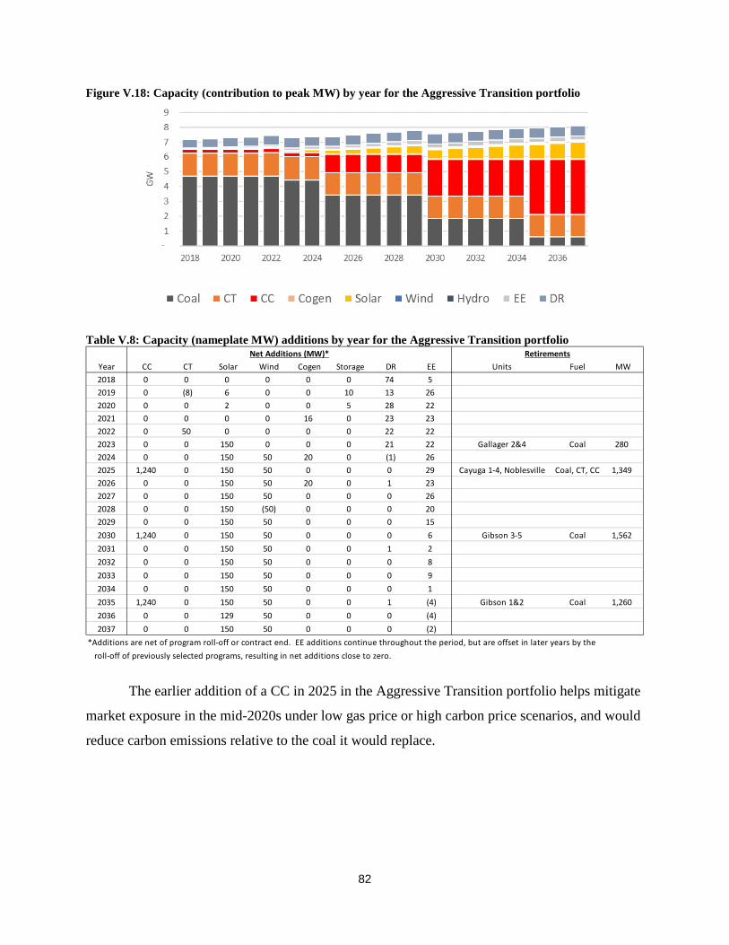
82

Figure V.18: Capacity (contribution to peak MW) by year for the Aggressive Transition portfolio

Table V.8: Capacity (nameplate MW) additions by year for the Aggressive Transition portfolio

The earlier addition of a CC in 2025 in the Aggressive Transition portfolio helps mitigate

market exposure in the mid-2020s under low gas price or high carbon price scenarios, and would

reduce carbon emissions relative to the coal it would replace.

Year CC CT Solar Wind Cogen Storage DR EE Units Fuel MW2018 0 0 0 0 0 0 74 52019 0 (8) 6 0 0 10 13 262020 0 0 2 0 0 5 28 222021 0 0 0 0 16 0 23 232022 0 50 0 0 0 0 22 222023 0 0 150 0 0 0 21 22 Gallager 2&4 Coal 2802024 0 0 150 50 20 0 (1) 262025 1,240 0 150 50 0 0 0 29 Cayuga 1-4, Noblesville Coal, CT, CC 1,3492026 0 0 150 50 20 0 1 232027 0 0 150 50 0 0 0 262028 0 0 150 (50) 0 0 0 202029 0 0 150 50 0 0 0 152030 1,240 0 150 50 0 0 0 6 Gibson 3-5 Coal 1,5622031 0 0 150 50 0 0 1 22032 0 0 150 50 0 0 0 82033 0 0 150 50 0 0 0 92034 0 0 150 50 0 0 0 12035 1,240 0 150 50 0 0 1 (4) Gibson 1&2 Coal 1,2602036 0 0 129 50 0 0 0 (4)2037 0 0 150 50 0 0 0 (2)

*Additions are net of program roll-off or contract end. EE additions continue throughout the period, but are offset in later years by the roll-off of previously selected programs, resulting in net additions close to zero.

Net Additions (MW)* Retirements

83

Figure V.19: Energy mix under all five scenarios for the Aggressive Transition portfolio

Rapid Decarbonization: CT

The Rapid Decarbonization: CT portfolio is modeled on the Aggressive Transition

portfolio in that the retirement schedule is the same, but with this portfolio we replace that retired

capacity almost entirely with renewables rather than including several gas-fired CCs. The first

CC is still added in 2025, but after that, wind and solar account for most other additions, with

just enough CT capacity added to meet the winter planning reserve margin requirement each

year.

- 5

10 15 20 25 30 35 40

2018 2021 2024 2027 2030 2033 2036

TWh

Reference Scenario, No Carbon Price

84

Figure V.20: Capacity (contribution to peak MW) by year for the Rapid Decarbonization: CT portfolio

Table V.9: Capacity (nameplate MW) additions by year for the Rapid Decarbonization: CT portfolio

The Rapid Decarbonization: CT portfolio includes a much greater proportion of low

variable cost resources (cost for renewables is almost entirely fixed and is mostly spent up front

on development and construction), making the energy mix much less sensitive to market

conditions. For that reason, the energy mix for the Rapid Decarbonization: CT portfolio looks

very similar across all five scenarios and there is little market exposure.

Year CC CT Solar Wind Cogen Storage DR EE Units Fuel MW2018 0 0 0 0 0 0 74 52019 0 (8) 6 0 0 10 13 262020 0 0 2 0 0 5 28 222021 0 0 0 0 16 0 23 232022 0 50 0 0 0 0 22 222023 0 0 150 0 0 0 21 22 Gallager 2&4 Coal 2802024 0 0 150 100 20 0 (1) 262025 1,240 0 200 100 0 0 0 29 Cayuga 1-4, Noblesville Coal, CT, CC 1,3492026 0 0 200 150 20 0 1 232027 0 0 250 150 0 0 0 262028 0 0 300 100 0 0 0 202029 0 0 400 250 0 0 0 152030 0 215 500 300 0 0 0 6 Gibson 3-5 Coal 1,5622031 0 0 100 350 0 0 1 22032 0 0 100 400 0 0 0 82033 0 0 400 450 0 0 0 92034 0 0 400 500 0 0 0 12035 0 645 400 500 0 0 1 (4) Gibson 1&2 Coal 1,2602036 0 0 (21) 0 0 0 0 (4)2037 0 0 0 0 0 0 0 (2)

*Additions are net of program roll-off or contract end. EE additions continue throughout the period, but are offset in later years by the roll-off of previously selected programs, resulting in net additions close to zero.

Net Additions (MW)* Retirements

85

Figure V.21: Energy mix under all five scenarios for the Rapid Decarbonization: CT portfolio

Rapid Decarbonization: Batteries

The Rapid Decarbonization: Batteries portfolio is designed to take the analysis one step

further and explore how the portfolio would perform if we used battery storage instead of CTs to

bolster the winter reserve margin. The retirements follow the same schedule as the Aggressive

Transition portfolio, and the first CC is still added in 2025, but after that all supply-side resource

additions are wind, solar, and batteries.

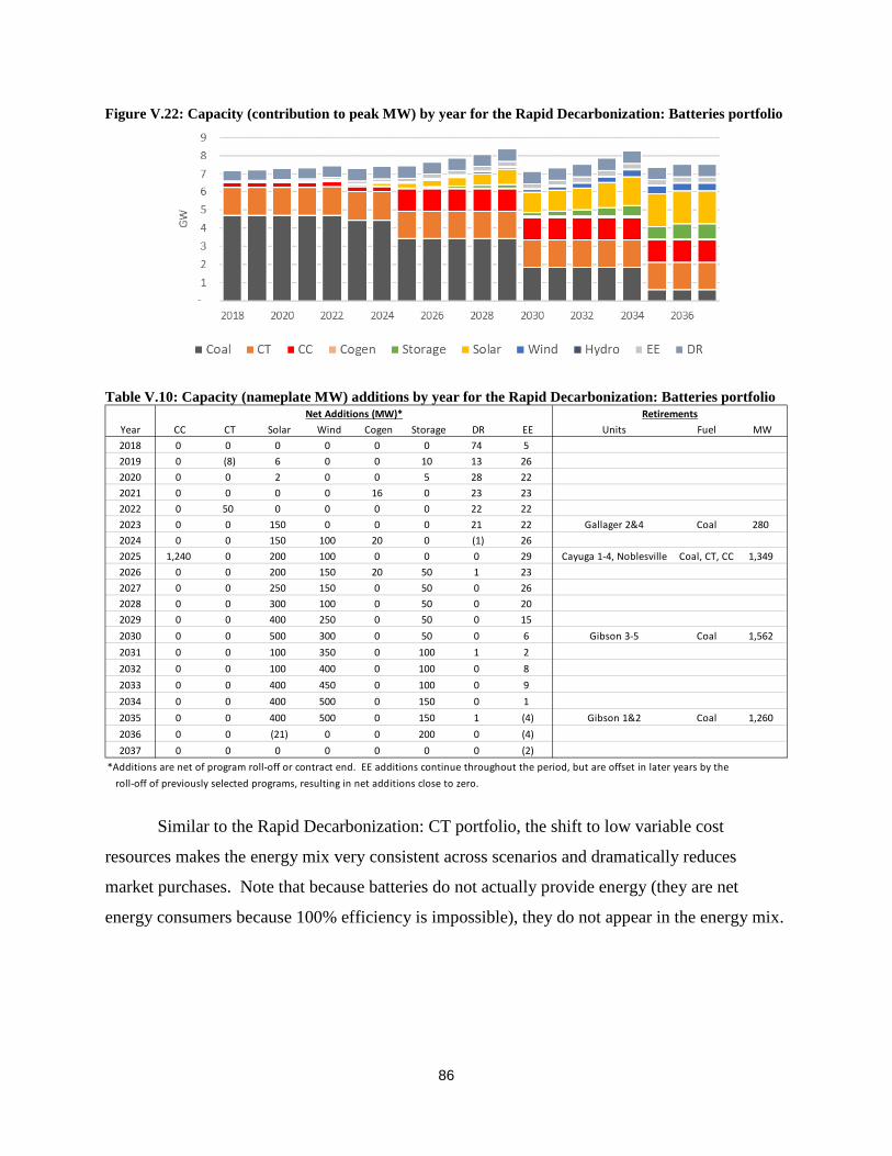
86

Figure V.22: Capacity (contribution to peak MW) by year for the Rapid Decarbonization: Batteries portfolio

Table V.10: Capacity (nameplate MW) additions by year for the Rapid Decarbonization: Batteries portfolio

Similar to the Rapid Decarbonization: CT portfolio, the shift to low variable cost

resources makes the energy mix very consistent across scenarios and dramatically reduces

market purchases. Note that because batteries do not actually provide energy (they are net

energy consumers because 100% efficiency is impossible), they do not appear in the energy mix.

Year CC CT Solar Wind Cogen Storage DR EE Units Fuel MW2018 0 0 0 0 0 0 74 52019 0 (8) 6 0 0 10 13 262020 0 0 2 0 0 5 28 222021 0 0 0 0 16 0 23 232022 0 50 0 0 0 0 22 222023 0 0 150 0 0 0 21 22 Gallager 2&4 Coal 2802024 0 0 150 100 20 0 (1) 262025 1,240 0 200 100 0 0 0 29 Cayuga 1-4, Noblesville Coal, CT, CC 1,3492026 0 0 200 150 20 50 1 232027 0 0 250 150 0 50 0 262028 0 0 300 100 0 50 0 202029 0 0 400 250 0 50 0 152030 0 0 500 300 0 50 0 6 Gibson 3-5 Coal 1,5622031 0 0 100 350 0 100 1 22032 0 0 100 400 0 100 0 82033 0 0 400 450 0 100 0 92034 0 0 400 500 0 150 0 12035 0 0 400 500 0 150 1 (4) Gibson 1&2 Coal 1,2602036 0 0 (21) 0 0 200 0 (4)2037 0 0 0 0 0 0 0 (2)

*Additions are net of program roll-off or contract end. EE additions continue throughout the period, but are offset in later years by the roll-off of previously selected programs, resulting in net additions close to zero.

Net Additions (MW)* Retirements

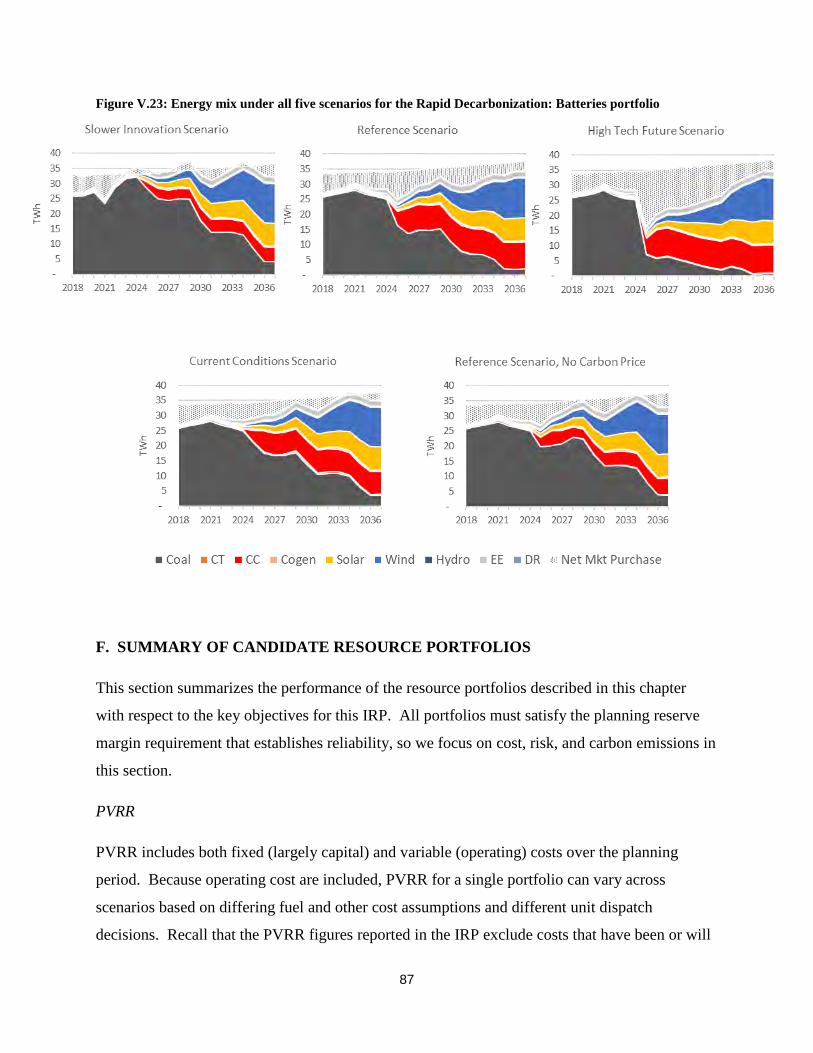
87

Figure V.23: Energy mix under all five scenarios for the Rapid Decarbonization: Batteries portfolio

F. SUMMARY OF CANDIDATE RESOURCE PORTFOLIOS

This section summarizes the performance of the resource portfolios described in this chapter

with respect to the key objectives for this IRP. All portfolios must satisfy the planning reserve

margin requirement that establishes reliability, so we focus on cost, risk, and carbon emissions in

this section.

PVRR

PVRR includes both fixed (largely capital) and variable (operating) costs over the planning

period. Because operating cost are included, PVRR for a single portfolio can vary across

scenarios based on differing fuel and other cost assumptions and different unit dispatch

decisions. Recall that the PVRR figures reported in the IRP exclude costs that have been or will

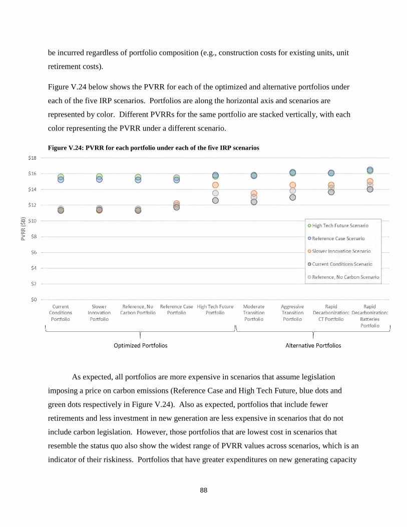
88

be incurred regardless of portfolio composition (e.g., construction costs for existing units, unit

retirement costs).

Figure V.24 below shows the PVRR for each of the optimized and alternative portfolios under

each of the five IRP scenarios. Portfolios are along the horizontal axis and scenarios are

represented by color. Different PVRRs for the same portfolio are stacked vertically, with each

color representing the PVRR under a different scenario.

Figure V.24: PVRR for each portfolio under each of the five IRP scenarios

As expected, all portfolios are more expensive in scenarios that assume legislation

imposing a price on carbon emissions (Reference Case and High Tech Future, blue dots and

green dots respectively in Figure V.24). Also as expected, portfolios that include fewer

retirements and less investment in new generation are less expensive in scenarios that do not

include carbon legislation. However, those portfolios that are lowest cost in scenarios that

resemble the status quo also show the widest range of PVRR values across scenarios, which is an

indicator of their riskiness. Portfolios that have greater expenditures on new generating capacity

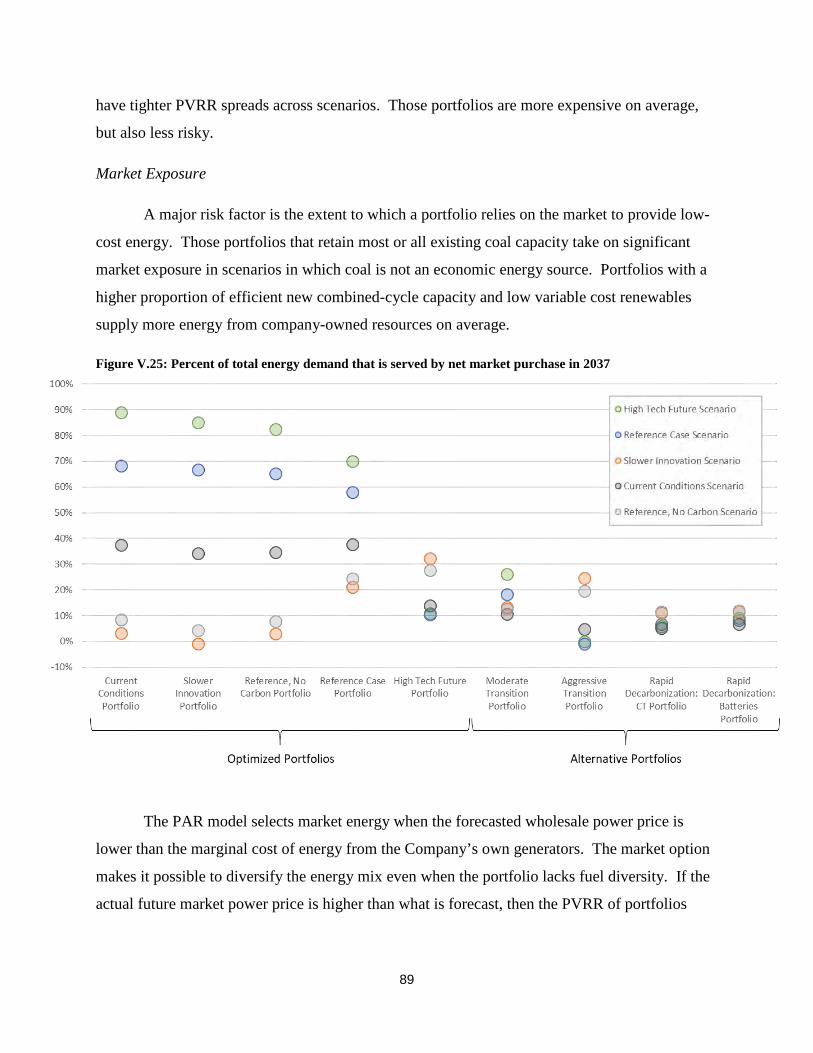
89

have tighter PVRR spreads across scenarios. Those portfolios are more expensive on average,

but also less risky.

Market Exposure

A major risk factor is the extent to which a portfolio relies on the market to provide low-

cost energy. Those portfolios that retain most or all existing coal capacity take on significant

market exposure in scenarios in which coal is not an economic energy source. Portfolios with a

higher proportion of efficient new combined-cycle capacity and low variable cost renewables

supply more energy from company-owned resources on average.

Figure V.25: Percent of total energy demand that is served by net market purchase in 2037

The PAR model selects market energy when the forecasted wholesale power price is

lower than the marginal cost of energy from the Company’s own generators. The market option

makes it possible to diversify the energy mix even when the portfolio lacks fuel diversity. If the

actual future market power price is higher than what is forecast, then the PVRR of portfolios

90

with substantial market exposure would also rise. Any cost increase would be capped at the cost

of meeting all energy demand with the company’s own resources.

Access to the MISO energy market also allows the Company to run the generating fleet

as efficiently as possible, even when doing so does not perfectly serve load. It can be costly to

meet rapid fluctuations in demand with coal units, and the market can be a cost-effective

alternative to doing so. Higher-than-forecast power prices limit this benefit.

To quantify the risk associated with relying on the market, we conducted additional PAR

model runs that did not include the market as an energy source. This simulates a situation in

which the wholesale power price is consistently above the cost of energy from the Company’s

own resources. Figure V.26 below shows how much the PVRR of each portfolio would increase

without recourse to the market.

Figure V.26: PVRR increase when market energy is prohibitively expensive

The portfolios optimized for the Current Conditions, Slower Innovation, Reference Case

Without Carbon Legislation, and Reference Case scenarios show the largest cost increases on

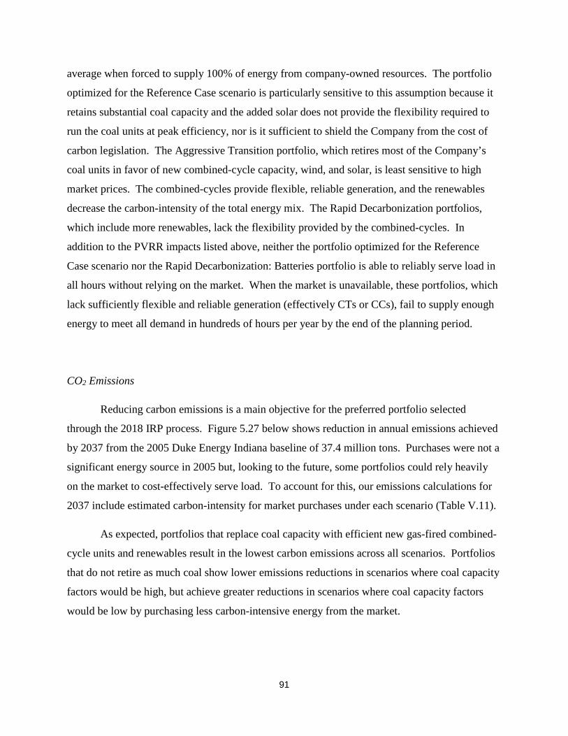
91

average when forced to supply 100% of energy from company-owned resources. The portfolio

optimized for the Reference Case scenario is particularly sensitive to this assumption because it

retains substantial coal capacity and the added solar does not provide the flexibility required to

run the coal units at peak efficiency, nor is it sufficient to shield the Company from the cost of

carbon legislation. The Aggressive Transition portfolio, which retires most of the Company’s

coal units in favor of new combined-cycle capacity, wind, and solar, is least sensitive to high

market prices. The combined-cycles provide flexible, reliable generation, and the renewables

decrease the carbon-intensity of the total energy mix. The Rapid Decarbonization portfolios,

which include more renewables, lack the flexibility provided by the combined-cycles. In

addition to the PVRR impacts listed above, neither the portfolio optimized for the Reference

Case scenario nor the Rapid Decarbonization: Batteries portfolio is able to reliably serve load in

all hours without relying on the market. When the market is unavailable, these portfolios, which

lack sufficiently flexible and reliable generation (effectively CTs or CCs), fail to supply enough

energy to meet all demand in hundreds of hours per year by the end of the planning period.

CO2 Emissions

Reducing carbon emissions is a main objective for the preferred portfolio selected

through the 2018 IRP process. Figure 5.27 below shows reduction in annual emissions achieved

by 2037 from the 2005 Duke Energy Indiana baseline of 37.4 million tons. Purchases were not a

significant energy source in 2005 but, looking to the future, some portfolios could rely heavily

on the market to cost-effectively serve load. To account for this, our emissions calculations for

2037 include estimated carbon-intensity for market purchases under each scenario (Table V.11).

As expected, portfolios that replace coal capacity with efficient new gas-fired combined-

cycle units and renewables result in the lowest carbon emissions across all scenarios. Portfolios

that do not retire as much coal show lower emissions reductions in scenarios where coal capacity

factors would be high, but achieve greater reductions in scenarios where coal capacity factors

would be low by purchasing less carbon-intensive energy from the market.

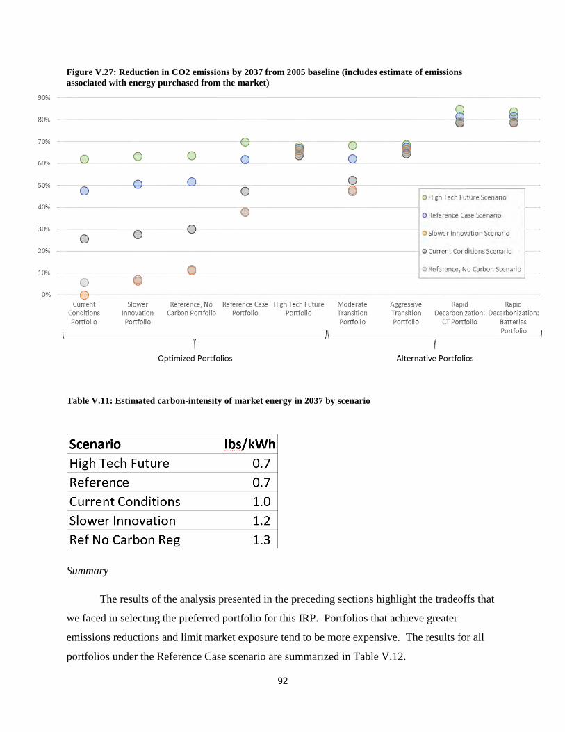
92

Figure V.27: Reduction in CO2 emissions by 2037 from 2005 baseline (includes estimate of emissions associated with energy purchased from the market)

Table V.11: Estimated carbon-intensity of market energy in 2037 by scenario

Summary

The results of the analysis presented in the preceding sections highlight the tradeoffs that

we faced in selecting the preferred portfolio for this IRP. Portfolios that achieve greater

emissions reductions and limit market exposure tend to be more expensive. The results for all

portfolios under the Reference Case scenario are summarized in Table V.12.

93

Table V.12: Summary of key results under Reference Case scenario

Portfolio PVRR ($B)

Energy from Market in 2037

(% of total energy)

CO2 Emissions Reduction from 2005

Baseline

Current Conditions $15.3 68% 48%

Slower Innovation $15.3 67% 51%

Reference, No Carbon $15.2 65% 52%

Reference Case $15.2 58% 62%

High Tech Future $15.8 10% 67%

Moderate Transition $15.8 18% 62%

Aggressive Transition $16.2 -1% 68%

Rapid Decarbonization: CT $16.1 7% 81%

Rapid Decarbonization: Batteries $16.5 8% 82%

OPT

IMIZ

EDAL

TERN

ATIV

E

94

SECTION VI: PREFERRED PORTFOLIO FOR 2018 INTEGRATED RESOURCE

PLAN

A. PREFERRED PORTFOLIO

We have selected the Moderate Transition portfolio described in Chapter V as the

preferred portfolio for the 2018 IRP. The energy and capacity mixes for this portfolio are shown

in Figures V.16 and V.17. Based on the results of our analysis discussed in Chapter 5, Section F,

we have concluded that this portfolio best balances the objectives of the 2018 IRP. Figure VI.1

shows the range of outcomes for the Moderate Transition portfolio across all scenarios (blue)

embedded in the range of outcomes for all portfolios across all scenarios (gray) under the three

key objectives we targeted for this IRP. The costs (PVRR) of this portfolio fall near the middle

of the range for all portfolios, while the market exposure (portion of total energy demand served

by the market by the end of the planning period) falls near the bottom of the range, and the

carbon emissions reduction (by the end of the planning period against the 2005 baseline) falls

near the top of the range for all portfolios. Under the Moderate Transition portfolio, the resource

mix will be diversified over time without committing to dramatic resource changes prematurely,

preserving decision-making flexibility going into the 2021 IRP analysis and shielding customers

from undue cost increases in the near-term. Duke Energy Indiana and its parent corporation

expect to maintain strong financial positions into the future and will be able to finance the

potential investments contemplated under the preferred portfolio.

95

Figure VI.1: Performance of Moderate Transition portfolio across all scenarios with respect to main IRP objectives (blue) within range of performance for all portfolios across all scenarios (gray)

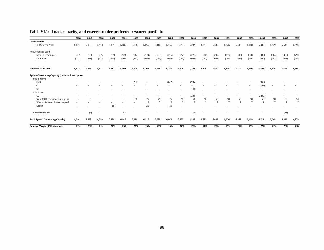
96

Table VI.1: Load, capacity, and reserves under preferred resource portfolio

2018 2019 2020 2021 2022 2023 2024 2025 2026 2027 2028 2029 2030 2031 2032 2033 2034 2035 2036 2037Load Forecast

DEI System Peak 6,031 6,000 6,110 6,051 6,086 6,136 6,056 6,114 6,166 6,213 6,237 6,297 6,339 6,376 6,403 6,460 6,499 6,529 6,543 6,593

Reductions to LoadNew EE Programs (27) (53) (75) (99) (123) (147) (174) (203) (226) (252) (271) (286) (292) (293) (300) (308) (309) (304) (300) (298) DR + IVVC (577) (591) (618) (640) (662) (685) (684) (683) (684) (683) (684) (685) (687) (688) (684) (684) (686) (687) (687) (689)

Adjusted Peak Load 5,427 5,356 5,417 5,312 5,302 5,304 5,197 5,228 5,256 5,278 5,282 5,326 5,360 5,395 5,419 5,469 5,503 5,538 5,556 5,606

System Generating Capacity (contribution to peak)Retirements

Coal - - - - - (280) - - (622) - (995) - - - - - (940) - - - CC - - - - - - - - - - - - - - - - (264) - - - CT - - - - - - - - - - (90) - - - - - - - - -

AdditionsCC - - - - - - - - - - 1,240 - - - - - 1,240 - - - Solar (50% contribution to peak) - 3 1 - - 50 75 75 75 50 50 50 50 50 50 50 50 50 50 50 Wind (13% contribution to peak - - - - - - 7 7 7 7 7 7 7 7 7 7 7 7 7 7 Cogen - - - 16 - - 20 - 20 - - - - - - - - - - -

Contract Rolloff - (8) - - 50 - - - - - (10) - - - - - - - (11) -

Total System Generating Capacity 6,584 6,579 6,580 6,596 6,646 6,416 6,517 6,599 6,078 6,135 6,336 6,393 6,449 6,506 6,562 6,619 6,711 6,768 6,814 6,870

Reserve Margin (15% minimum) 21% 23% 21% 24% 25% 21% 25% 26% 16% 16% 20% 20% 20% 21% 21% 21% 22% 22% 23% 23%

97

B. SHORT-TERM ACTION PLAN

The preferred portfolio for the 2018 IRP calls for little change through 2021. We will implement

the EE programs approved under Cause No. 43955 DSM-4, we will complete approximately 8

MW of new solar capacity that is currently in development, and a contract to purchase 8 MW of

CT capacity will expire. Additionally, we will install a total of approximately 15 MW of battery

energy storage systems at Crane Naval Station, the Indiana National Guard’s Camp Atterbury,

and a substation in Nabb, Indiana, providing grid support and backup power to critical facilities.

C. PREFERRED PORTFOLIOS ABILITY TO ADAPT TO CHANGING CONDITIONS

One of the benefits of increasing the diversity of the generating fleet is the increased flexibility

that can be leveraged in the face of a changing world. Given the measured pace of transition, the

company can adjust its plans accordingly. For example, if load grows more or less than

expected, the plan could adjust by accelerating or slowing down implementation of the preferred

portfolio. If the relative cost of a resource should change from what is being evaluated in this

IRP, the company can take advantage of resources with improved economics and move away

from those resources whose relative economics have worsened. This could happen due a

resources capital costs, O&M costs, environmental compliance costs, or other regulatory

requirements

D. VARIABLES TO MONITOR AND ONGOING IMPROVEMENTS TO IRP PROCESS

While the preferred portfolio for the 2018 IRP includes resource choices specified

through 2037, it is important to remember that resource planning is an ongoing, iterative process.

Every three years we reassess the state of our operating environment and adjust our plans

accordingly. The IRP will be updated again in 2021, at which time we will adapt the resource

selections based on new forecasts and technical, market, and political insights. Key factors to

monitor ahead of the 2021 IRP will be:

• The outcome of the 2020 elections

• Renewable energy and carbon policy at the state and local levels

• The cost trends for solar, wind, and batteries

• The evolution of MISO market rules for renewables and storage

98

• Natural gas prices

In addition to tracking factors external to the company, we are working on improving our

IRP analysis in the following ways:

• More detailed load forecasting informed by data from advanced meters

• Adoption of new modeling tools better equipped to capture the complexities of

the changing power industry

• Improved cost forecasting for supply-side resources

99

The Duke Energy Indiana 2018 Integrated Resource Plan July 1, 2019

Appendix A: Financial & Operating Forecasts For Preferred Portfolio

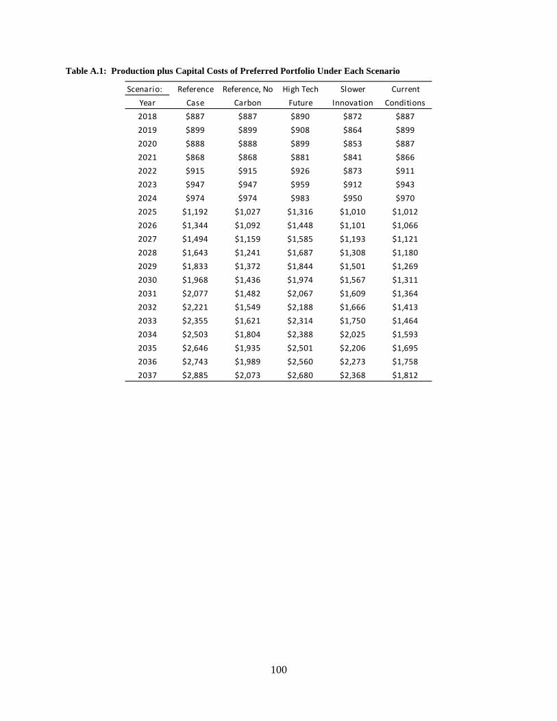
100

Table A.1: Production plus Capital Costs of Preferred Portfolio Under Each Scenario

Scenario: Reference Reference, No High Tech Slower CurrentYear Case Carbon Future Innovation Conditions2018 $887 $887 $890 $872 $8872019 $899 $899 $908 $864 $8992020 $888 $888 $899 $853 $8872021 $868 $868 $881 $841 $8662022 $915 $915 $926 $873 $9112023 $947 $947 $959 $912 $9432024 $974 $974 $983 $950 $9702025 $1,192 $1,027 $1,316 $1,010 $1,0122026 $1,344 $1,092 $1,448 $1,101 $1,0662027 $1,494 $1,159 $1,585 $1,193 $1,1212028 $1,643 $1,241 $1,687 $1,308 $1,1802029 $1,833 $1,372 $1,844 $1,501 $1,2692030 $1,968 $1,436 $1,974 $1,567 $1,3112031 $2,077 $1,482 $2,067 $1,609 $1,3642032 $2,221 $1,549 $2,188 $1,666 $1,4132033 $2,355 $1,621 $2,314 $1,750 $1,4642034 $2,503 $1,804 $2,388 $2,025 $1,5932035 $2,646 $1,935 $2,501 $2,206 $1,6952036 $2,743 $1,989 $2,560 $2,273 $1,7582037 $2,885 $2,073 $2,680 $2,368 $1,812

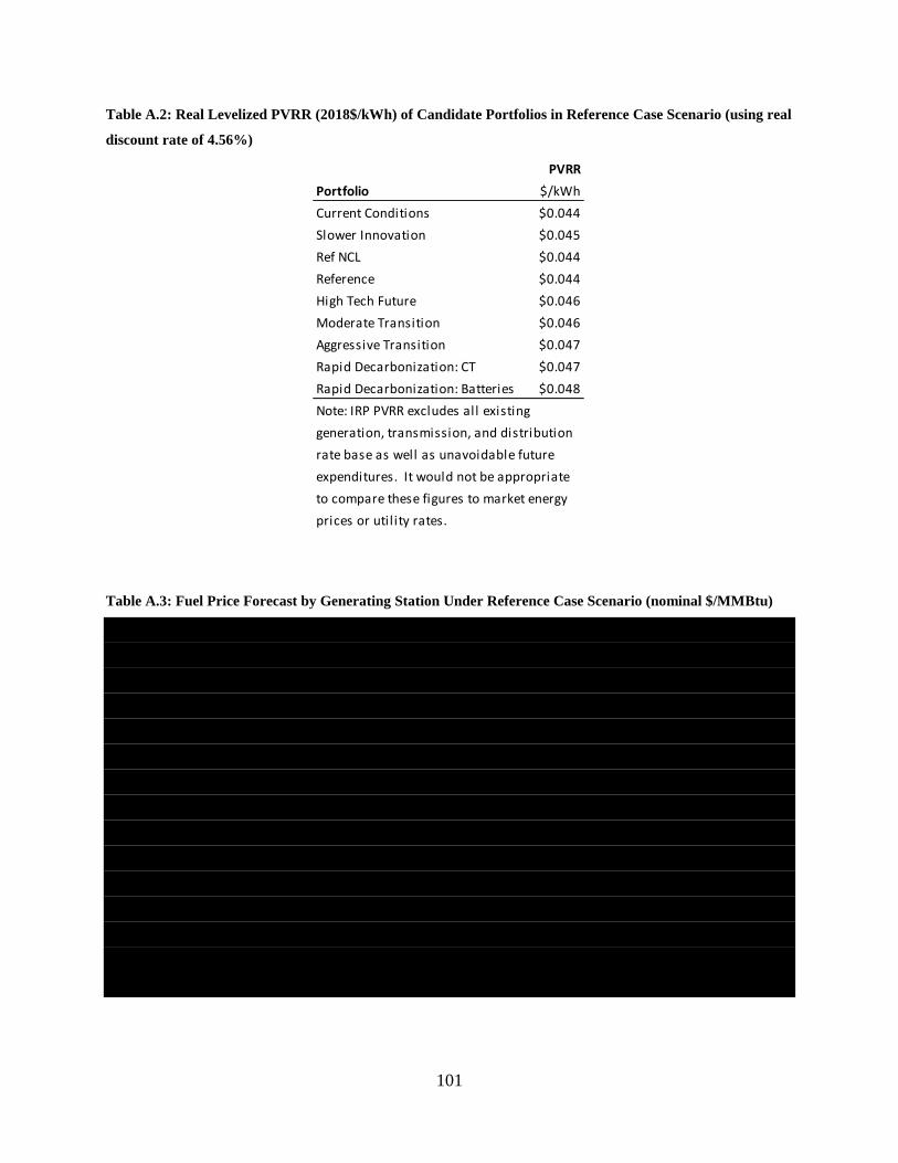
101

Table A.2: Real Levelized PVRR (2018$/kWh) of Candidate Portfolios in Reference Case Scenario (using real

discount rate of 4.56%)

Table A.3: Fuel Price Forecast by Generating Station Under Reference Case Scenario (nominal $/MMBtu)

PVRRPortfolio $/kWhCurrent Conditions $0.044Slower Innovation $0.045Ref NCL $0.044Reference $0.044High Tech Future $0.046Moderate Transition $0.046Aggressive Transition $0.047Rapid Decarbonization: CT $0.047Rapid Decarbonization: Batteries $0.048Note: IRP PVRR excludes all existinggeneration, transmission, and distributionrate base as well as unavoidable futureexpenditures. It would not be appropriateto compare these figures to market energyprices or util ity rates.

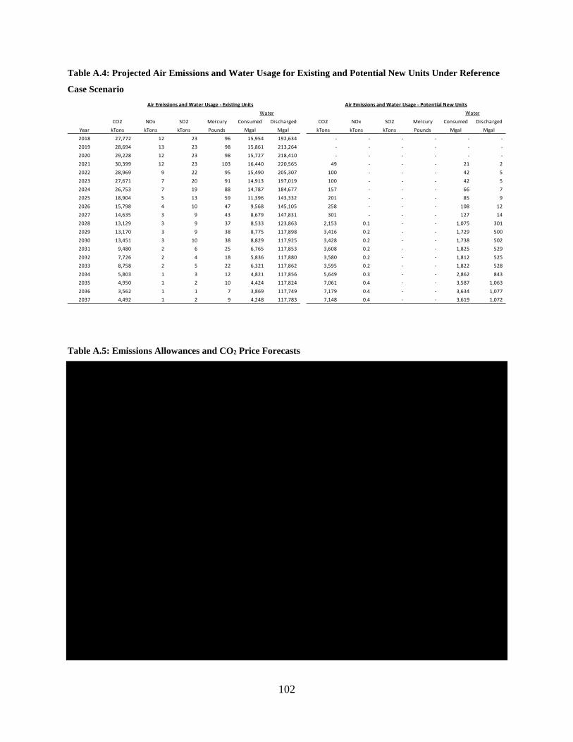
102

Table A.4: Projected Air Emissions and Water Usage for Existing and Potential New Units Under Reference

Case Scenario

Table A.5: Emissions Allowances and CO2 Price Forecasts

CO2 NOx SO2 Mercury Consumed Discharged CO2 NOx SO2 Mercury Consumed DischargedYear kTons kTons kTons Pounds Mgal Mgal kTons kTons kTons Pounds Mgal Mgal2018 27,772 12 23 96 15,954 192,634 - - - - - - 2019 28,694 13 23 98 15,861 213,264 - - - - - - 2020 29,228 12 23 98 15,727 218,410 - - - - - - 2021 30,399 12 23 103 16,440 220,565 49 - - - 21 2 2022 28,969 9 22 95 15,490 205,307 100 - - - 42 5 2023 27,671 7 20 91 14,913 197,019 100 - - - 42 5 2024 26,753 7 19 88 14,787 184,677 157 - - - 66 7 2025 18,904 5 13 59 11,396 143,332 201 - - - 85 9 2026 15,798 4 10 47 9,568 145,105 258 - - - 108 12 2027 14,635 3 9 43 8,679 147,831 301 - - - 127 14 2028 13,129 3 9 37 8,533 123,863 2,153 0.1 - - 1,075 301 2029 13,170 3 9 38 8,775 117,898 3,416 0.2 - - 1,729 500 2030 13,451 3 10 38 8,829 117,925 3,428 0.2 - - 1,738 502 2031 9,480 2 6 25 6,765 117,853 3,608 0.2 - - 1,825 529 2032 7,726 2 4 18 5,836 117,880 3,580 0.2 - - 1,812 525 2033 8,758 2 5 22 6,321 117,862 3,595 0.2 - - 1,822 528 2034 5,803 1 3 12 4,821 117,856 5,649 0.3 - - 2,862 843 2035 4,950 1 2 10 4,424 117,824 7,061 0.4 - - 3,587 1,063 2036 3,562 1 1 7 3,869 117,749 7,179 0.4 - - 3,634 1,077 2037 4,492 1 2 9 4,248 117,783 7,148 0.4 - - 3,619 1,072

Water WaterAir Emissions and Water Usage - Potential New UnitsAir Emissions and Water Usage - Existing Units

Year Annual NOx Seasonal NOx2 Annual SO2 Reference Slower Innovation High Tech Future2018 $3.50 $160.00 $2.50 $0.00 $0.00 $0.002019 $3.50 $160.00 $2.50 $0.00 $0.00 $0.002020 $3.50 $160.00 $2.50 $0.00 $0.00 $0.002021 $3.50 $160.00 $2.50 $0.00 $0.00 $0.002022 $3.50 $160.00 $2.50 $0.00 $0.00 $0.002023 $3.50 $160.00 $2.50 $0.00 $0.00 $0.002024 $3.50 $163.20 $2.55 $0.00 $0.00 $0.002025 $3.57 $166.46 $2.60 $5.00 $0.00 $10.002026 $3.64 $169.79 $2.65 $8.00 $0.00 $13.002027 $3.71 $173.19 $2.71 $11.00 $0.00 $16.002028 $3.79 $176.65 $2.76 $14.00 $0.00 $19.002029 $3.86 $180.19 $2.82 $17.00 $0.00 $22.002030 $3.94 $183.79 $2.87 $20.00 $0.00 $25.002031 $4.02 $187.47 $2.93 $23.00 $0.00 $28.002032 $4.10 $191.21 $2.99 $26.00 $0.00 $31.002033 $4.18 $195.04 $3.05 $29.00 $0.00 $34.002034 $4.27 $198.94 $3.11 $32.00 $0.00 $37.002035 $4.35 $202.92 $3.17 $35.00 $0.00 $40.002036 $4.44 $206.98 $3.23 $38.00 $0.00 $43.002037 $4.53 $211.12 $3.30 $41.00 $0.00 $46.00

1.) 2018-2028: CommodityXL pricing, escalated at 2%/year after 20282.) Seasonal NOx allowances cover May-September of each year

NOx and SO2 Price Forecasts ($/ton)1 CO2 Price Forecasts ($/ton)

103

The Duke Energy Indiana 2018 Integrated Resource Plan July 1, 2019

Appendix B: Load Forecast

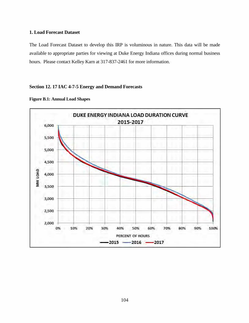
104

1. Load Forecast Dataset

The Load Forecast Dataset to develop this IRP is voluminous in nature. This data will be made

available to appropriate parties for viewing at Duke Energy Indiana offices during normal business

hours. Please contact Kelley Karn at 317-837-2461 for more information.

Section 12. 17 IAC 4-7-5 Energy and Demand Forecasts

Figure B.1: Annual Load Shapes

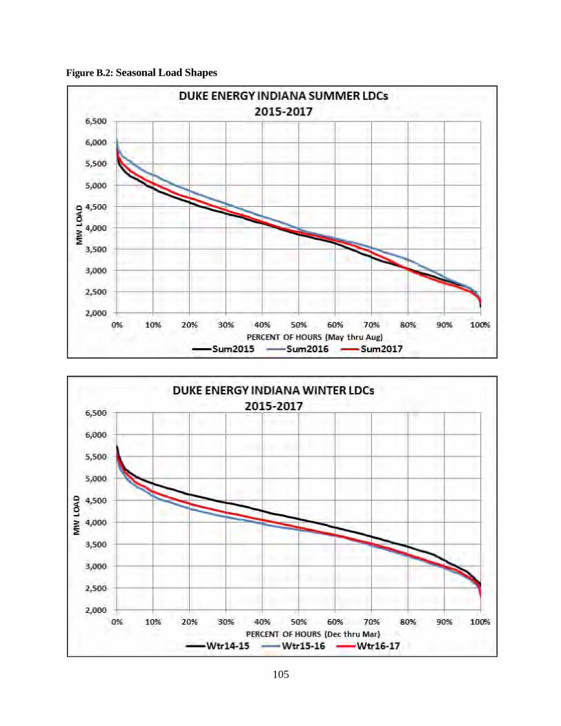
105

Figure B.2: Seasonal Load Shapes

106

Figure B.3: Monthly Load Shapes

107

Figure B.3: Monthly Load Shapes (con’t.)

108

Figure B.4: Selected Weekly Load Shapes

109

Figure B.4: Selected Weekly Load Shapes (con’t.)

2,000

2,500

3,000

3,500

4,000

4,500

5,000

5,500

6,000

6,500

7,000

1 25 49 73 97 121 145

MW

LO

AD

HOURS

DUKE ENERGY INDIANA - FALL WEEKLY LOAD SHAPE SUNDAY OCT 1 - SATURDAY OCT 7, 2017

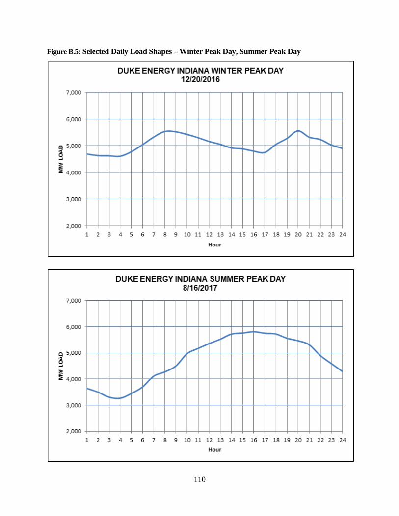
110

Figure B.5: Selected Daily Load Shapes – Winter Peak Day, Summer Peak Day

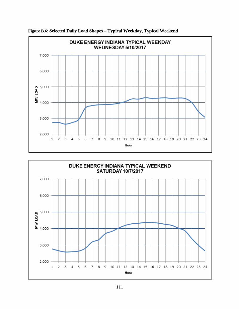
111

Figure B.6: Selected Daily Load Shapes – Typical Weekday, Typical Weekend

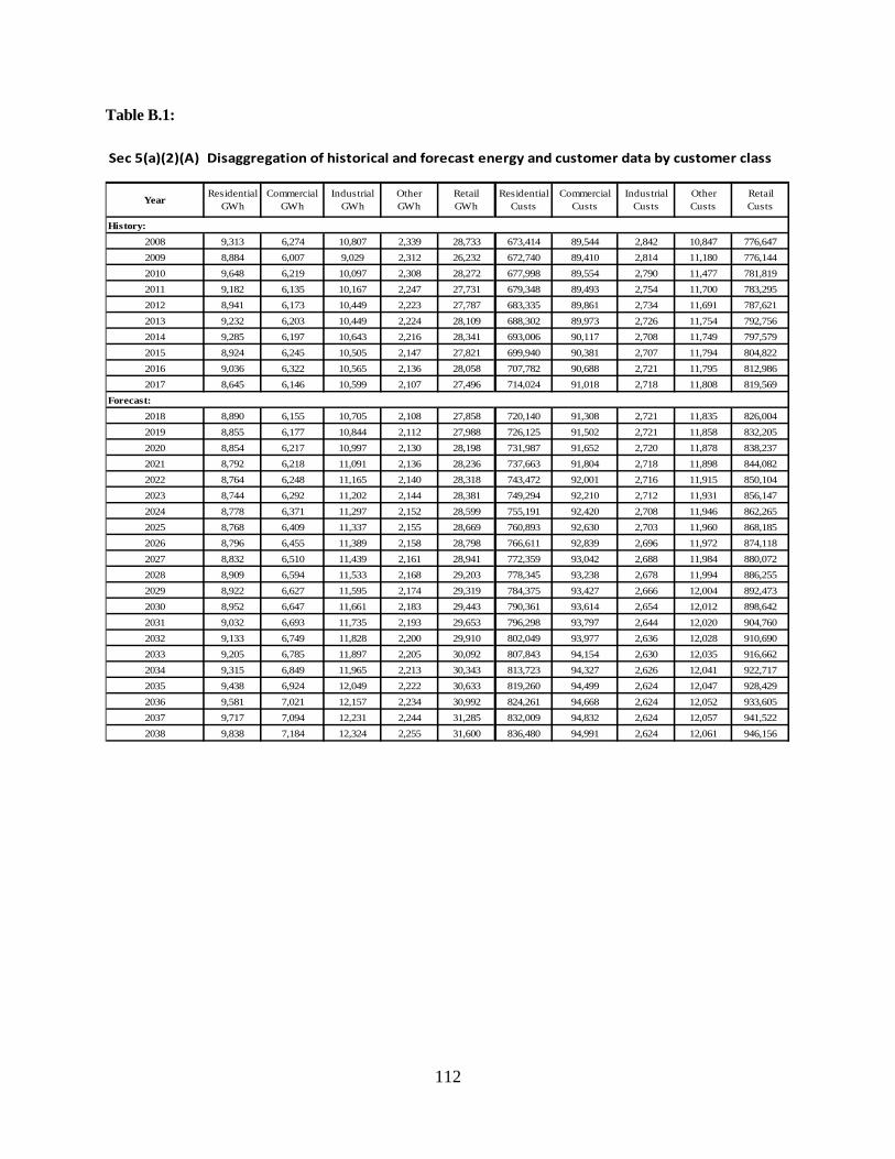
112

Table B.1:

Sec 5(a)(2)(A) Disaggregation of historical and forecast energy and customer data by customer class

History:2008 9,313 6,274 10,807 2,339 28,733 673,414 89,544 2,842 10,847 776,6472009 8,884 6,007 9,029 2,312 26,232 672,740 89,410 2,814 11,180 776,1442010 9,648 6,219 10,097 2,308 28,272 677,998 89,554 2,790 11,477 781,8192011 9,182 6,135 10,167 2,247 27,731 679,348 89,493 2,754 11,700 783,2952012 8,941 6,173 10,449 2,223 27,787 683,335 89,861 2,734 11,691 787,6212013 9,232 6,203 10,449 2,224 28,109 688,302 89,973 2,726 11,754 792,7562014 9,285 6,197 10,643 2,216 28,341 693,006 90,117 2,708 11,749 797,5792015 8,924 6,245 10,505 2,147 27,821 699,940 90,381 2,707 11,794 804,8222016 9,036 6,322 10,565 2,136 28,058 707,782 90,688 2,721 11,795 812,9862017 8,645 6,146 10,599 2,107 27,496 714,024 91,018 2,718 11,808 819,569

Forecast:2018 8,890 6,155 10,705 2,108 27,858 720,140 91,308 2,721 11,835 826,0042019 8,855 6,177 10,844 2,112 27,988 726,125 91,502 2,721 11,858 832,2052020 8,854 6,217 10,997 2,130 28,198 731,987 91,652 2,720 11,878 838,2372021 8,792 6,218 11,091 2,136 28,236 737,663 91,804 2,718 11,898 844,0822022 8,764 6,248 11,165 2,140 28,318 743,472 92,001 2,716 11,915 850,1042023 8,744 6,292 11,202 2,144 28,381 749,294 92,210 2,712 11,931 856,1472024 8,778 6,371 11,297 2,152 28,599 755,191 92,420 2,708 11,946 862,2652025 8,768 6,409 11,337 2,155 28,669 760,893 92,630 2,703 11,960 868,1852026 8,796 6,455 11,389 2,158 28,798 766,611 92,839 2,696 11,972 874,1182027 8,832 6,510 11,439 2,161 28,941 772,359 93,042 2,688 11,984 880,0722028 8,909 6,594 11,533 2,168 29,203 778,345 93,238 2,678 11,994 886,2552029 8,922 6,627 11,595 2,174 29,319 784,375 93,427 2,666 12,004 892,4732030 8,952 6,647 11,661 2,183 29,443 790,361 93,614 2,654 12,012 898,6422031 9,032 6,693 11,735 2,193 29,653 796,298 93,797 2,644 12,020 904,7602032 9,133 6,749 11,828 2,200 29,910 802,049 93,977 2,636 12,028 910,6902033 9,205 6,785 11,897 2,205 30,092 807,843 94,154 2,630 12,035 916,6622034 9,315 6,849 11,965 2,213 30,343 813,723 94,327 2,626 12,041 922,7172035 9,438 6,924 12,049 2,222 30,633 819,260 94,499 2,624 12,047 928,4292036 9,581 7,021 12,157 2,234 30,992 824,261 94,668 2,624 12,052 933,6052037 9,717 7,094 12,231 2,244 31,285 832,009 94,832 2,624 12,057 941,5222038 9,838 7,184 12,324 2,255 31,600 836,480 94,991 2,624 12,061 946,156

Commercial Custs

Industrial Custs

Other Custs

Retail CustsYear

Residential GWh

Commercial GWh

Industrial GWh

Other GWh

Retail GWh

Residential Custs

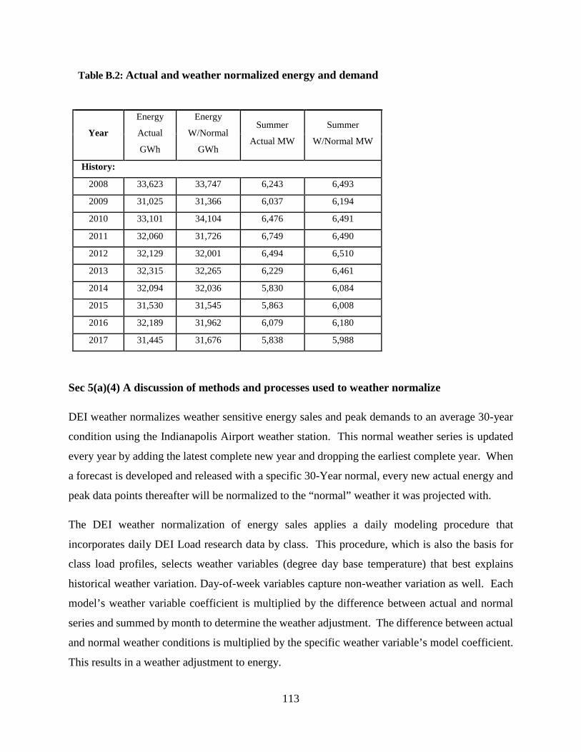
113

Table B.2: Actual and weather normalized energy and demand

Year

Energy

Actual

GWh

Energy

W/Normal

GWh

Summer

Actual MW

Summer

W/Normal MW

History:

2008 33,623 33,747 6,243 6,493

2009 31,025 31,366 6,037 6,194

2010 33,101 34,104 6,476 6,491

2011 32,060 31,726 6,749 6,490

2012 32,129 32,001 6,494 6,510

2013 32,315 32,265 6,229 6,461

2014 32,094 32,036 5,830 6,084

2015 31,530 31,545 5,863 6,008

2016 32,189 31,962 6,079 6,180

2017 31,445 31,676 5,838 5,988

Sec 5(a)(4) A discussion of methods and processes used to weather normalize

DEI weather normalizes weather sensitive energy sales and peak demands to an average 30-year

condition using the Indianapolis Airport weather station. This normal weather series is updated

every year by adding the latest complete new year and dropping the earliest complete year. When

a forecast is developed and released with a specific 30-Year normal, every new actual energy and

peak data points thereafter will be normalized to the “normal” weather it was projected with.

The DEI weather normalization of energy sales applies a daily modeling procedure that

incorporates daily DEI Load research data by class. This procedure, which is also the basis for

class load profiles, selects weather variables (degree day base temperature) that best explains

historical weather variation. Day-of-week variables capture non-weather variation as well. Each

model’s weather variable coefficient is multiplied by the difference between actual and normal

series and summed by month to determine the weather adjustment. The difference between actual

and normal weather conditions is multiplied by the specific weather variable’s model coefficient.

This results in a weather adjustment to energy.

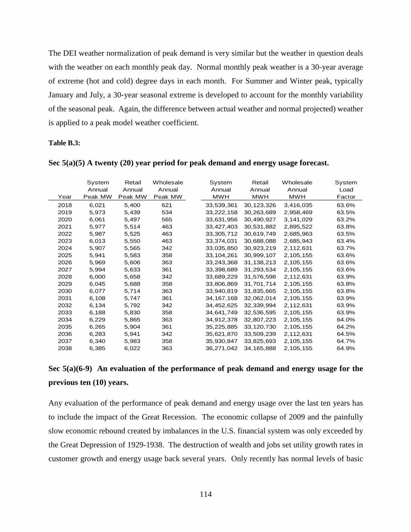
114

The DEI weather normalization of peak demand is very similar but the weather in question deals

with the weather on each monthly peak day. Normal monthly peak weather is a 30-year average

of extreme (hot and cold) degree days in each month. For Summer and Winter peak, typically

January and July, a 30-year seasonal extreme is developed to account for the monthly variability

of the seasonal peak. Again, the difference between actual weather and normal projected) weather

is applied to a peak model weather coefficient.

Table B.3:

Sec 5(a)(5) A twenty (20) year period for peak demand and energy usage forecast.

Sec 5(a)(6-9) An evaluation of the performance of peak demand and energy usage for the

previous ten (10) years.

Any evaluation of the performance of peak demand and energy usage over the last ten years has

to include the impact of the Great Recession. The economic collapse of 2009 and the painfully

slow economic rebound created by imbalances in the U.S. financial system was only exceeded by

the Great Depression of 1929-1938. The destruction of wealth and jobs set utility growth rates in

customer growth and energy usage back several years. Only recently has normal levels of basic

Year

System Annual

Peak MW

Retail Annual

Peak MW

Wholesale Annual

Peak MW

System Annual MWH

Retail Annual MWH

Wholesale Annual MWH

System Load

Factor2018 6,021 5,400 621 33,539,361 30,123,326 3,416,035 63.6%2019 5,973 5,439 534 33,222,158 30,263,689 2,958,469 63.5%2020 6,061 5,497 565 33,631,956 30,490,927 3,141,029 63.2%2021 5,977 5,514 463 33,427,403 30,531,882 2,895,522 63.8%2022 5,987 5,525 463 33,305,712 30,619,749 2,685,963 63.5%2023 6,013 5,550 463 33,374,031 30,688,088 2,685,943 63.4%2024 5,907 5,565 342 33,035,850 30,923,219 2,112,631 63.7%2025 5,941 5,583 358 33,104,261 30,999,107 2,105,155 63.6%2026 5,969 5,606 363 33,243,368 31,138,213 2,105,155 63.6%2027 5,994 5,633 361 33,398,689 31,293,534 2,105,155 63.6%2028 6,000 5,658 342 33,689,229 31,576,598 2,112,631 63.9%2029 6,045 5,688 358 33,806,869 31,701,714 2,105,155 63.8%2030 6,077 5,714 363 33,940,819 31,835,665 2,105,155 63.8%2031 6,108 5,747 361 34,167,168 32,062,014 2,105,155 63.9%2032 6,134 5,792 342 34,452,625 32,339,994 2,112,631 63.9%2033 6,188 5,830 358 34,641,749 32,536,595 2,105,155 63.9%2034 6,229 5,865 363 34,912,378 32,807,223 2,105,155 64.0%2035 6,265 5,904 361 35,225,885 33,120,730 2,105,155 64.2%2036 6,283 5,941 342 35,621,870 33,509,239 2,112,631 64.5%2037 6,340 5,983 358 35,930,847 33,825,693 2,105,155 64.7%2038 6,385 6,022 363 36,271,042 34,165,888 2,105,155 64.9%

115

economic growth stimulated any semblance of growth in energy sales and customer growth for

DEI.

A second industry event occurring over the last ten years that must be mentioned is the availability

of merchant generation. Cheap natural gas (central station or customer self-service) generation

and subsidized renewable generation has resulted in low-cost generation options for Sales for

Resale or wholesale service municipals and cooperatives. DEI has gone through a material drop

in Sales for Resale.

A third factor impacting the level of growth in DEI peak and energy sales is the adoption of

federally mandated highly efficient residential and commercial sector appliances and utility

sponsored programs offered to help spur more efficient use of electricity. DEI has observed that

the residential and commercial classes are more likely to participate in utility energy efficiency

programs with the current legislative landscape in Indiana for large industrial customers enabled

to opt-out of EE programs. Industrial customers are able to implement their own cost saving

efforts, measures which result in reducing both, kWh usage and billing demand charges.

Each of these events have worked to reduce electric energy sales growth and even shrink the

average annual kWh use per residential customer for several years. It forced DEI to move to the

Itron SAE (Statistically Adjusted End-use) forecast methodology. We have found this approach

to best capture the changing levels of more efficient appliances saturating through the residential

households and commercial class end-uses.

While DEI has been projecting impacts of roof-top solar and electric vehicles upon the energy and

peak demand projections for several years, there are improvements in the works applying actual

(more local) solar load shapes and EV “charging time” data to improve our understand these

influences upon class hourly load shapes.

Sec 5(b)(1-3) An evaluation of plausible risk boundaries or alternative forecasts of peak

demand and energy use.

DEI will often perform a High-Low scenario around a Base Case. All three projections were

centered around three economic scenarios developed in January 2018 by Moody’s Analytics. The

publishing address for Moody’s Analytics is 121 North Walnut Street, West Chester, PA 19380.

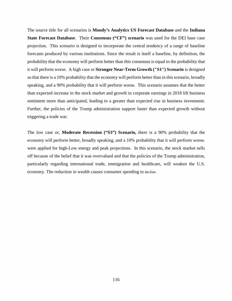
116

The source title for all scenarios is Moody’s Analytics US Forecast Database and the Indiana

State Forecast Database. Their Consensus (“CF”) scenario was used for the DEI base case

projection. This scenario is designed to incorporate the central tendency of a range of baseline

forecasts produced by various institutions. Since the result is itself a baseline, by definition, the

probability that the economy will perform better than this consensus is equal to the probability that

it will perform worse. A high case or Stronger Near-Term Growth ("S1") Scenario is designed

so that there is a 10% probability that the economy will perform better than in this scenario, broadly

speaking, and a 90% probability that it will perform worse. This scenario assumes that the better

than expected increase in the stock market and growth in corporate earnings in 2018 lift business

sentiment more than anticipated, leading to a greater than expected rise in business investment.

Further, the policies of the Trump administration support faster than expected growth without

triggering a trade war.

The low case or, Moderate Recession (“S3”) Scenario, there is a 90% probability that the

economy will perform better, broadly speaking, and a 10% probability that it will perform worse.

were applied for high-Low energy and peak projections. In this scenario, the stock market sells

off because of the belief that it was overvalued and that the policies of the Trump administration,

particularly regarding international trade, immigration and healthcare, will weaken the U.S.

economy. The reduction in wealth causes consumer spending to decline.

117

Table B.:

The scenario results above reflect the application of each scenario’s specific economic input series

into the base case model.

Year Low Base High Year Low Base High2018 33,110,064 -1.3% 33,539,361 0.3% 33,650,983 2018 5,932 -1.5% 6,021 0.4% 6,044 2019 32,103,505 -3.4% 33,222,158 0.9% 33,513,261 2019 5,768 -3.4% 5,973 0.9% 6,028 2020 32,630,633 -3.0% 33,631,956 1.0% 33,974,686 2020 5,885 -2.9% 6,061 1.0% 6,125 2021 32,604,637 -2.5% 33,427,403 1.1% 33,809,855 2021 5,831 -2.4% 5,977 1.2% 6,048 2022 32,505,611 -2.4% 33,305,712 1.2% 33,720,074 2022 5,844 -2.4% 5,987 1.3% 6,064 2023 32,564,919 -2.4% 33,374,031 1.3% 33,805,313 2023 5,868 -2.4% 6,013 1.3% 6,092 2024 32,188,762 -2.6% 33,035,850 1.4% 33,492,186 2024 5,755 -2.6% 5,907 1.4% 5,991 2025 32,228,469 -2.6% 33,104,261 1.5% 33,591,467 2025 5,783 -2.7% 5,941 1.5% 6,031 2026 32,343,278 -2.7% 33,243,368 1.5% 33,751,774 2026 5,807 -2.7% 5,969 1.6% 6,063 2027 32,477,272 -2.8% 33,398,689 1.6% 33,923,472 2027 5,828 -2.8% 5,994 1.6% 6,091 2028 32,745,050 -2.8% 33,689,229 1.6% 34,231,612 2028 5,830 -2.8% 6,000 1.7% 6,101 2029 32,847,699 -2.8% 33,806,869 1.7% 34,365,140 2029 5,874 -2.8% 6,045 1.7% 6,148 2030 32,967,855 -2.9% 33,940,819 1.7% 34,508,326 2030 5,903 -2.9% 6,077 1.7% 6,182 2031 33,179,930 -2.9% 34,167,168 1.7% 34,750,009 2031 5,931 -2.9% 6,108 1.8% 6,216 2032 33,450,809 -2.9% 34,452,625 1.7% 35,054,600 2032 5,954 -2.9% 6,134 1.8% 6,244 2033 33,623,841 -2.9% 34,641,749 1.8% 35,256,586 2033 6,004 -3.0% 6,188 1.8% 6,301 2034 33,878,385 -3.0% 34,912,378 1.8% 35,540,762 2034 6,042 -3.0% 6,229 1.9% 6,344 2035 34,175,361 -3.0% 35,225,885 1.8% 35,869,840 2035 6,075 -3.0% 6,265 1.9% 6,384 2036 34,550,822 -3.0% 35,621,870 1.8% 36,279,141 2036 6,089 -3.1% 6,283 1.9% 6,404 2037 34,841,657 -3.0% 35,930,847 1.9% 36,600,702 2037 6,143 -3.1% 6,340 2.0% 6,465 2038 35,162,682 -3.1% 36,271,042 1.9% 36,956,508 2038 6,184 -3.1% 6,385 2.0% 6,513

CAGR: CAGR:2018-38 0.3% 0.4% 0.5% 2018-38 0.2% 0.3% 0.4%

Annual System Requirements (MWH) Annual System Peak (MW)

Sec 5(b)(1-3) Low - Base - High Energy & Peak Scenarios

118

The Duke Energy Indiana 2018 Integrated Resource Plan July 1, 2019

Appendix C: Supply-Side Resources

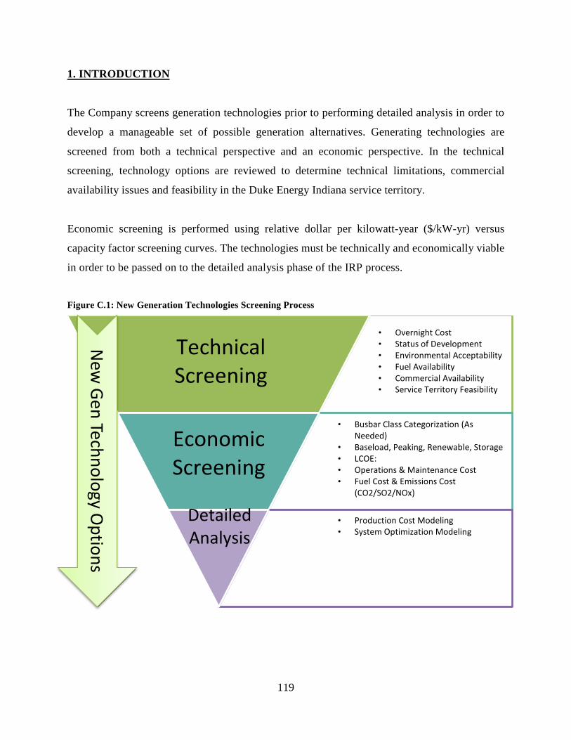
119

1. INTRODUCTION

The Company screens generation technologies prior to performing detailed analysis in order to

develop a manageable set of possible generation alternatives. Generating technologies are

screened from both a technical perspective and an economic perspective. In the technical

screening, technology options are reviewed to determine technical limitations, commercial

availability issues and feasibility in the Duke Energy Indiana service territory.

Economic screening is performed using relative dollar per kilowatt-year ($/kW-yr) versus

capacity factor screening curves. The technologies must be technically and economically viable

in order to be passed on to the detailed analysis phase of the IRP process.

Figure C.1: New Generation Technologies Screening Process

New

Gen Technology Options

Technical Screening

Economic Screening

Detailed Analysis

• Overnight Cost • Status of Development • Environmental Acceptability • Fuel Availability • Commercial Availability • Service Territory Feasibility

• Busbar Class Categorization (As Needed)

• Baseload, Peaking, Renewable, Storage • LCOE: • Operations & Maintenance Cost • Fuel Cost & Emissions Cost

(CO2/SO2/NOx)

• Production Cost Modeling • System Optimization Modeling

120

2. TECHNICAL SCREENING

The first step in the Company’s supply-side screening process for the IRP is a technical screening of

the technologies to eliminate those that have technical limitations, commercial availability issues, or

are cannot feasibly serve the Duke Energy Indiana service territory. A brief explanation of the

technologies excluded at this point and the basis for their exclusion follows:

• Geothermal was eliminated because there are no suitable geothermal resources in the

region to develop into a power generation project.

Figure C.2: Geothermal Map of the US (Source: NREL)

• Pumped Storage Hydropower (PSH) is the only conventional, mature, commercial,

utility-scale electricity storage option available currently. This technology consumes

off-peak electricity by pumping water from a lower reservoir to an upper reservoir.

When the electric grid needs more electricity and when electricity prices are higher,

121

water is released from the upper reservoir. As the water flows from the upper reservoir

to the lower reservoir, it goes through a hydroelectric turbine to generate electricity.

Many operational pumped storage hydropower plants are providing electric reliability

and reserves for the electric grid in high demand situations. PSH can provide a high

amount of power because its only limitation is the capacity of the upper reservoir.

Typically, these plants can be as large as 4,000 MW and have an efficiency of 76% -

85% (EPRI, 2012). Therefore, this technology is effective at meeting electric demand

and transmission overload by shifting, storing, and producing electricity. This is

important because an increasing supply of intermittent renewable energy generation

such as solar will cause challenges to the electric grid. PSH installations are greatly

dependent on regional geography and face several challenges including: environmental

impact concerns, a long permitting process, and a relatively high initial capital cost.

There are no suitable sites for PSH in the Duke Energy Indiana service territory.

• Compressed Air Energy Storage (CAES), although demonstrated on a utility scale

and generally commercially available, is not a widely applied technology and remains

relatively expensive. Traditional systems require a suitable storage site, commonly

underground where the compressed air is used to boost the output of a gas turbine. The

high capital requirements for these resources arise from the fact that suitable sites that

possess the proper geological formations and conditions necessary for the compressed

air storage reservoir are relatively scarce, especially in the Indiana. However, above-

ground compressed air energy storage (AGCAES) technologies are under development

but at a much smaller scale, approximately 0.5 - 20MW. Several companies have

attempted to develop cost effective CAES systems using above ground storage tanks.

Most attempts to date have not been commercially successful, but their development is

being monitored.

122

Figure C.3: CAES Potential US Salt Cavern Site Depiction (Source: NETL)

• Liquid Air Energy Storage (LAES) uses electricity to cool air until it liquefies, stores

the liquid air in a tank, brings the liquid air back to a gaseous state (by exposure to

ambient air or with waste heat from an industrial process) and uses that gas to turn a

turbine and generate electricity. Although demonstrated through several pilot projects,

the scaling of this technology and the resultant economics is not yet completely

understood. As research and pilots continues with LAES, Duke Energy will continue

to monitor as the technology offers bulk energy storage without the need for reservoir

construction.

• Small Modular Nuclear Reactors (SMR) are generally defined as having capabilities

of less than 300 MW per reactor and possessing the ability for the major nuclear island

components to be fully manufactured in a facility, thus reducing onsite construction

costs. A SMR vendor is undergoing the process to obtain a Design Certification with

the NRC while several other vendors perform Pre-Application work. A vendor has

successfully received a reduction in the Emergency Planning Zone (EPZ) area, which

greatly reduces the land and subsequent security requirement to support operation.

Several Early Site Permits are under evaluation by the NRC for SMR development,

123

one in Idaho and another in Tennessee. Duke Energy will be monitoring the progress

of these SMR projects for potential consideration and evaluation for future resource

plans as they provide an emission free source of fuel diverse, flexible generation.

• Fuel Cells, although originally envisioned as being a competitor for combustion

turbines and central power plants, are now targeted to mostly distributed power

generation systems. The size of the distributed generation applications ranges from a

few kW to tens of MW in the long-term. Cost and performance issues have generally

limited their application to niche markets and/or subsidized installations. While a

medium level of research and development continues, this technology is not

commercially viable/available for utility-scale application.

• Supercritical CO2 Brayton Cycle, an advanced heat recovery system that utilizes

liquid carbon dioxide to obtain much higher efficiencies than the traditional Rankine

Cycle used in power conversion systems, is of increasing interest. However, the

technology is not mature or ready for commercialization. Several pilots are underway

and Duke Energy will continue to monitor their development as a potential source of

future generation needs.

• Offshore Wind was eliminated because there are no suitable offshore locations for

Indiana.

• Solar Steam Augmentation systems utilize solar thermal energy to supplement a

Rankine steam cycle such as that in a fossil generating plant. The supplemental steam

could be integrated into the steam cycle and support additional MW generation similar

in concept to the purpose of duct firing a heat recovery steam generator. This

technology, although attractive, has several hurdles yet to clear, including a clean

operating history and initial capital cost reductions. This technology is very site-

specific and Duke Energy will continue to monitor developments in the area of steam

augmentation.

124

A brief explanation of the technology additions for 2018 and the basis for their inclusion follows:

• Addition of Battery Storage Options to the IRP

Energy storage solutions are becoming a viable tool in support of grid stability at peak demand

times and in support of energy shifting and smoothing from renewable sources. Energy Storage

in the form of battery storage is becoming more feasible with the advances in battery technology

(Tesla Lithium-ion battery technology) and the reduction in battery cost; however, their uses (even

within Duke Energy) have been concentrated on frequency regulation, solar smoothing, and/or

energy shifting from localized renewable energy sources with a high incidence of intermittency

(i.e. solar and wind applications). In order to generically evaluate the potential value of a

generation-connected battery storage system an unencumbered battery dedicated to capacity and

energy services will be utilized for screening purposes. Encumbrances to the battery are other

uses which may limit, or even completely eliminate the battery system's ability to provide capacity

and energy storage services. These encumbrances may include (but are not limited to) frequency

response, asset deferral, back-up power, black start, ancillary services, etc. Duke Energy

recognizes the potential benefits that battery connected systems can provide, especially at the

transmission and distribution (T&D) levels, which reside outside the scope of this IRP. Evaluation

of potential T&D benefits, along with other uses that can be "stacked" with these T&D benefits,

are being assessed on a case-by-case basis at this time through pilot projects.

Duke Energy has several projects in operation since 2011, mainly in support of regulating output

voltages/frequencies from renewable energy sources to the grid. Each of these applications

supports frequency regulation, solar smoothing, or energy shifting from a local solar array.

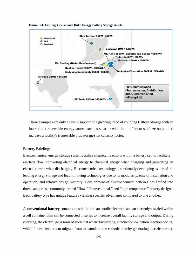
125

Figure C.4: Existing, Operational Duke Energy Battery Storage Assets

These examples are only a few in support of a growing trend of coupling Battery Storage with an

intermittent renewable energy source such as solar or wind in an effort to stabilize output and

increase a facility's (renewable plus storage) net capacity factor.

Battery Briefing:

Electrochemical energy storage systems utilize chemical reactions within a battery cell to facilitate

electron flow, converting electrical energy to chemical energy when charging and generating an

electric current when discharging. Electrochemical technology is continually developing as one of the

leading energy storage and load following technologies due to its modularity, ease of installation and

operation, and relative design maturity. Development of electrochemical batteries has shifted into

three categories, commonly termed “flow,” “conventional,” and “high temperature” battery designs.

Each battery type has unique features yielding specific advantages compared to one another.

A conventional battery contains a cathodic and an anodic electrode and an electrolyte sealed within

a cell container than can be connected in series to increase overall facility storage and output. During

charging, the electrolyte is ionized such that when discharging, a reduction-oxidation reaction occurs,

which forces electrons to migrate from the anode to the cathode thereby generating electric current.

126

Batteries are designated by the electro-chemicals utilized within the cell; the most popular

conventional batteries are lead acid and lithium ion type batteries.

Lead acid batteries are the most mature and commercially accessible battery technology, as their

design has undergone considerable development since conceptualized in the late 1800s. The

Department of Energy (DOE) estimates there is approximately 110 MW of lead acid battery storage

currently installed worldwide. Although lead acid batteries require relatively low capital cost, this

technology also has inherently high maintenance costs and handling issues associated with toxicity

as well as low energy density (yields higher land and civil work requirements). Lead acid batteries

also have a relatively short life cycle at 5 to 10 years, especially when used in high cycling

applications.

Lithium ion (Li-ion) batteries contain graphite and metal-oxide electrodes and lithium ions dissolved

within an organic electrolyte. The movement of lithium ions during cell charge and discharge

generates current. Li-ion technology has seen a resurgence of development in recent years due to its

high energy density, low self-discharge, and cycling tolerance. Many Li-ion manufacturers currently

offer 15-year warranties or performance guarantees. Consequently, Li- ion has gained traction in

several markets including the utility and automotive industries.

Li-ion battery prices are trending downward, and continued development and investment by

manufacturers are expected to further reduce production costs. While there is still a wide range of

project cost expectations due to market uncertainty, Li-ion batteries are anticipated to expand their

reach in the utility market sector. At present, Li-ion Battery Technology is the only battery technology

considered for the 2018 IRP based are market maturity and ease of commercialization.

Flow batteries utilize an electrode cell stack with externally stored electrolyte material. The flow

battery is comprised of positive and negative electrode cell stacks separated by a selectively

permeable ion exchange membrane. The charge-inducing chemical reaction occurs in liquid

electrolyte storage tanks, which hold the stored energy until discharge is required. Various control

and pumped circulation systems complete the flow battery system in which the cells can be stacked

in series to achieve the desired voltage difference.

127

The battery is charged as the liquid electrolytes are pumped through the electrode cell stacks, which

serve only as a catalyst and transport medium to the ion-inducing chemical reaction. The excess

positive ions at the anode are allowed through the ion-selective membrane to maintain

electroneutrality at the cathode, which experiences a buildup of negative ions. The charged electrolyte

solution is circulated back to storage tanks until the process is allowed to repeat in reverse for

discharge as necessary.

In addition to external electrolyte storage, flow batteries differ from traditional batteries in that energy

conversion occurs as a direct result of the reduction-oxidation reactions occurring in the electrolyte

solution itself. The electrode is not a component of the electrochemical fuel and does not participate

in the chemical reaction. Therefore, the electrodes are not subject to the same deterioration that

depletes electrical performance of traditional batteries, resulting in high cycling life of the flow

battery. Flow batteries are also scalable such that energy storage capacity is determined by the size of

the electrolyte storage tanks, allowing the system to approach its theoretical energy density. Flow

batteries are typically less capital intensive than some conventional batteries but require additional

installation and operation costs associated with balance of plant equipment.

High temperature batteries operate similarly to conventional batteries, but they utilize molten salt

electrodes and carry the added advantage that high temperature operation can yield heat for other

applications simultaneously. The technology is considered mature with ongoing commercial

development at the grid level. The most popular and technically developed high temperature option

is the Sodium Sulfur (NaS) battery. Japan-based NGK Insulators, the largest NaS battery

manufacturer, recently installed a 4 MW system in Presidio, Texas in 2010 following operation of

systems totaling more than 160 MW since the project’s inception in the 1980s.

The NaS battery is typically a hermetically sealed cell that consists of a molten sulfur electrolyte at

the cathode and molten sodium electrolyte at the anode, separated by a Beta-alumina ceramic

membrane and enclosed in an aluminum casing. The membrane is selectively permeable only to

positive sodium ions, which are created from the oxidation of sodium metal and pass through to

combine with sulfur resulting in the formation of sodium polysulfides. As power is supplied to the

128

battery in charging, the sodium ions are dissociated from the polysulfides and forced back through

the membrane to re-form elemental sodium. The melting points of sodium and sulfur are

approximately 98oC and 113oC, respectively. To maintain the electrolytes in liquid form and for

optimal performance, the NaS battery systems are typically operated and stored at around 300oC,

which results in a higher self-discharge rate of 14 percent to 18 percent. For this reason, these systems

are usually designed for use in high-cycling applications and longer discharge durations.

NaS systems are expected to have an operable life of around 15 years and are one of the most

developed chemical energy storage technologies. However, unlike other battery types, costs of NaS

systems have historically held, making other options more commercially viable at present.

Generation Flexibility

As more intermittent generation becomes associated with the system, there may be a greater need for

generation that has rapid load changing capabilities. This generation would need to be dispatchable,

possess desirable capacity/energy, and ramp at a desired rate. Some of the technologies that have

'technically' screened in possess these qualities or have the potential to in the near future. Effort is

being made to value the characteristics of flexibility and quantify that value to the system. As a result

of the flexible generation need, some features of 'generic' plant's base designs have been modified to

reflect the change in cost and performance to accomplish a more desired plant characteristic to

diminish the impact of the intermittent generation additions.

129

Tables C.1: 12x24 Energy Production Profiles for Wind and Solar Resources

3. ECONOMIC SCREENING

The Company selected the technologies listed below for the screening analysis in System Optimizer

(SO) for the Duke Energy Indiana territory. While regulation may effectively preclude new coal-fired

generation, Duke Energy Indiana has included ultra-supercritical pulverized coal (USCPC) with

carbon capture sequestration (CCS) and integrated gasification combined cycle (IGCC) technologies

with CCS of 1400 pounds/net MWh capture rate as options for base load analysis consistent with the

potential federal regulation standards. Additional detail on the expected impacts from EPA

regulations to new coal-fired options is included in Appendix F. 2018 additions include Combined

Heat & Power (CHP) as a base load technology and Lithium ion Battery Storage as a renewable

technology.

Dispatchable

• Base load – 782 MW Ultra-Supercritical Pulverized Coal with CCS

• Base load – 557 MW 2x1 IGCC with CCS

• Base load – 2 x 1,117 MW Nuclear Units

• Base load – 1,239 MW – 2x2x1 Advanced Combined Cycle (CC) (Fired)

SOLAR Hour EndMonth 1 2 3 4 5 6 7 8 9 10 11 12 13 14 15 16 17 18 19 20 21 22 23 24January 0% 0% 0% 0% 0% 0% 0% 0% 6% 28% 36% 34% 34% 35% 38% 45% 30% 6% 0% 0% 0% 0% 0% 0%February 0% 0% 0% 0% 0% 0% 0% 1% 21% 48% 50% 46% 44% 48% 54% 64% 62% 25% 1% 0% 0% 0% 0% 0%March 0% 0% 0% 0% 0% 0% 0% 1% 17% 47% 54% 63% 65% 64% 62% 60% 55% 44% 26% 4% 0% 0% 0% 0%April 0% 0% 0% 0% 0% 0% 0% 3% 35% 64% 66% 70% 71% 72% 74% 70% 66% 62% 52% 16% 0% 0% 0% 0%May 0% 0% 0% 0% 0% 0% 0% 13% 43% 58% 62% 68% 73% 73% 75% 72% 69% 61% 47% 25% 2% 0% 0% 0%June 0% 0% 0% 0% 0% 0% 1% 14% 38% 56% 67% 72% 77% 78% 78% 77% 76% 74% 64% 33% 8% 0% 0% 0%July 0% 0% 0% 0% 0% 0% 0% 14% 49% 64% 74% 76% 79% 78% 80% 79% 76% 72% 58% 37% 6% 0% 0% 0%August 0% 0% 0% 0% 0% 0% 0% 7% 36% 69% 77% 81% 81% 80% 79% 76% 76% 71% 55% 22% 2% 0% 0% 0%September 0% 0% 0% 0% 0% 0% 0% 2% 22% 56% 68% 69% 68% 67% 68% 69% 70% 64% 35% 7% 0% 0% 0% 0%October 0% 0% 0% 0% 0% 0% 0% 0% 8% 45% 60% 61% 59% 58% 57% 58% 55% 44% 10% 0% 0% 0% 0% 0%November 0% 0% 0% 0% 0% 0% 0% 0% 14% 39% 44% 44% 45% 45% 46% 44% 21% 2% 0% 0% 0% 0% 0% 0%December 0% 0% 0% 0% 0% 0% 0% 0% 5% 22% 31% 31% 31% 32% 35% 36% 16% 0% 0% 0% 0% 0% 0% 0%

WIND Hour EndMonth 1 2 3 4 5 6 7 8 9 10 11 12 13 14 15 16 17 18 19 20 21 22 23 24January 55% 53% 52% 52% 52% 51% 51% 52% 51% 48% 44% 44% 43% 43% 44% 46% 44% 46% 47% 50% 52% 56% 56% 57%February 58% 53% 47% 46% 49% 53% 56% 54% 54% 50% 47% 45% 42% 46% 48% 49% 49% 47% 50% 54% 55% 53% 49% 52%March 50% 49% 47% 48% 53% 51% 53% 47% 40% 43% 44% 44% 47% 46% 44% 40% 42% 44% 43% 43% 43% 47% 48% 45%April 44% 39% 36% 44% 46% 43% 40% 32% 27% 27% 27% 30% 32% 36% 37% 37% 38% 35% 31% 31% 33% 36% 43% 44%May 29% 27% 30% 29% 28% 25% 22% 16% 17% 22% 24% 21% 21% 24% 28% 26% 32% 26% 23% 24% 23% 27% 26% 28%June 33% 33% 30% 28% 31% 31% 26% 18% 11% 11% 12% 15% 15% 15% 18% 19% 19% 19% 19% 19% 21% 26% 28% 27%July 27% 24% 24% 23% 24% 24% 20% 14% 5% 5% 7% 8% 11% 10% 11% 12% 14% 13% 8% 11% 19% 22% 24% 28%August 33% 35% 32% 30% 29% 25% 23% 18% 5% 4% 7% 9% 9% 14% 15% 16% 16% 17% 15% 22% 29% 36% 37% 38%September 50% 54% 50% 52% 51% 52% 50% 50% 37% 37% 41% 44% 42% 41% 45% 46% 43% 43% 42% 46% 50% 49% 46% 49%October 62% 59% 60% 60% 59% 55% 54% 54% 53% 40% 36% 34% 37% 38% 38% 37% 39% 43% 47% 54% 59% 61% 65% 66%November 55% 57% 54% 55% 60% 59% 56% 55% 55% 52% 49% 46% 48% 47% 45% 47% 46% 46% 50% 52% 55% 60% 59% 57%December 62% 59% 56% 61% 58% 54% 50% 47% 49% 48% 46% 45% 45% 43% 43% 46% 46% 49% 51% 54% 61% 64% 65% 64%

130

• Base load – 16 MW – Combined Heat & Power (CHP, CT driven)

• Peaking/Intermediate – 202 MW, 12 x Reciprocating Engine Plant

• Peaking/Intermediate – 858 MW 4 x F-Frame Combustion Turbines (CTs)

• Renewable – 2 MW Solar PV plus 2MW / 8MWh Li-ion Battery

Non-Dispatchable

• Renewable – 150 MW Wind - On-Shore

• Renewable – 150 MW Solar PV - Fixed Tilt

• Renewable – 5 MW / 20 MWh Li-ion Battery

Information Sources

The cost and performance data for each technology being screened is based on research and

information from several sources. These sources include, but may not be limited to the following

internal Departments: Duke Energy’s Project Management & Construction, Emerging Technologies,

and Corporate & Regulatory Strategy. The following external sources may also be utilized:

proprietary third-party engineering studies, the Electric Power Research Institute (EPRI) Technical

Assessment Guide (TAG®), and Energy Information Administration (EIA). In addition, fuel and

operating cost estimates are developed internally by Duke Energy, from other sources such as those

mentioned above, or a combination of the two. EPRI information or other information or estimates

from external studies are not site-specific but generally reflect the costs and operating parameters for

installation in the Midwest. Finally, every effort is made to ensure that capital, operating and

maintenance costs (O&M), fuel costs and other parameters are current and include similar scope

across the technologies being screened. The supply-side screening analysis uses the same fuel prices

for coal and natural gas as well as NOx, SO2, and CO2 allowance prices as those utilized downstream

in the detailed analysis (discussed in Appendix A).

131

4. CAPITAL COST FORECAST

A capital cost forecast was developed with support from a third party to project not only Renewables

and Battery Storage capital costs, but the costs of all generation technologies technically screened in.

The Technology Forecast Factors were sourced from the EIA’s Annual Energy Outlook (AEO) 2017

which provides costs projections for various technologies through the planning period as an input to

the National Energy Modeling System (NEMS) utilized by the EIA for the AEO.

Using 2018 as a base year, an "annual forecast factor is calculated based on the macroeconomic

variable tracking the metals and metal products producer price index, thereby creating a link between

construction costs and commodity prices." (NEMS Model Documentation 2016, July 2017)

From NEMS Model Documentation 2016, July 2017:

"Uncertainty about investment costs for new technologies is captured in the Electric Capacity

Planning module of NEMS (ECP) using technological optimism and learning factors.

• The technological optimism factor reflects the inherent tendency to underestimate costs for

new technologies. The degree of technological optimism depends on the complexity of the

engineering design and the stage of development. As development proceeds and more data

become available, cost estimates become more accurate and the technological optimism factor

declines.

• Learning factors represent reductions in capital costs due to learning-by-doing. Learning

factors are calculated separately for each of the major design components of the technology.

For new technologies, cost reductions due to learning also account for international

experience in building generating capacity. Generally, overnight costs for new, untested

components are assumed to decrease by a technology specific percentage for each doubling of

capacity for the first three doublings, by 10% for each of the next five doublings of capacity,

and by 1% for each further doubling of capacity. For mature components or conventional

designs, costs decrease by 1% for each doubling of capacity."

132

The resulting Forecast Factor Table developed from the EIA technology maturity curves for each

corresponding technology screened is depicted in Table C.2.

Table C.2: Excerpt from Forecast Factor Table by Technology (Source: EIA-AEO 2017)

These forecast factors were blended with additional third-party capital cost projections for more

rapidly developing technologies (i.e. Solar PV, Battery Storage) in order to provide a consistent

forecast through the planning period for all technologies evaluated. The resulting Capital Cost

changes for the technologies shown in Table C.1 are depicted below in Figure C.5.

Year

AeroCT

F Class FrameCT

J Class FrameCT RICE

Onshore Wind

1x1 J ClassCombined

Cycle

2x1 J ClassCombined

Cycle

2018 1.000 1.000 1.000 1.000 1.000 1.000 1.0002019 0.996 0.995 0.995 0.996 0.996 0.995 0.9952020 0.993 0.990 0.990 0.993 0.993 0.991 0.9902021 0.989 0.984 0.984 0.989 0.989 0.986 0.9842022 0.983 0.978 0.978 0.983 0.983 0.980 0.9782023 0.974 0.967 0.967 0.974 0.974 0.970 0.9672024 0.965 0.957 0.957 0.965 0.965 0.960 0.9572025 0.954 0.942 0.942 0.954 0.954 0.947 0.9422026 0.941 0.920 0.920 0.941 0.941 0.928 0.9202027 0.928 0.902 0.902 0.928 0.928 0.913 0.9022028 0.918 0.877 0.877 0.918 0.918 0.894 0.8772029 0.910 0.859 0.859 0.910 0.910 0.879 0.8592030 0.901 0.840 0.840 0.901 0.901 0.864 0.8402031 0.892 0.827 0.827 0.892 0.892 0.853 0.8272032 0.884 0.815 0.815 0.884 0.884 0.842 0.815

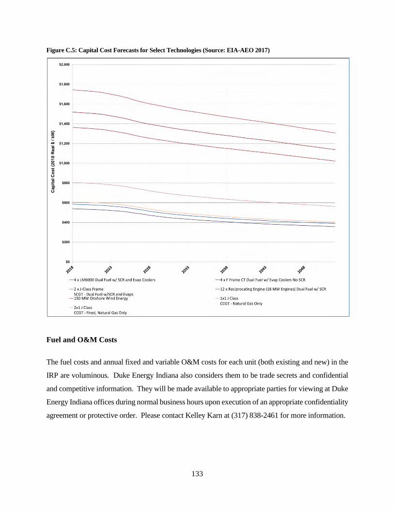
133

Figure C.5: Capital Cost Forecasts for Select Technologies (Source: EIA-AEO 2017)

Fuel and O&M Costs

The fuel costs and annual fixed and variable O&M costs for each unit (both existing and new) in the

IRP are voluminous. Duke Energy Indiana also considers them to be trade secrets and confidential

and competitive information. They will be made available to appropriate parties for viewing at Duke

Energy Indiana offices during normal business hours upon execution of an appropriate confidentiality

agreement or protective order. Please contact Kelley Karn at (317) 838-2461 for more information.

134

The Duke Energy Indiana 2018 Integrated Resource Plan July 1, 2019

Appendix D: Demand Side Resources

135

ENERGY EFFICIENCY RESOURCES

A. INTRODUCTION

As part of the IRP, Duke Energy Indiana analyzes the impacts associated with new Energy

Efficiency (EE) or Demand Response (DR) programs and any changes to existing EE or DR

measures/programs. The portfolio of existing and future EE and DR measures/programs is

evaluated within the IRP to examine the impact on the generation plan if the current set of

measures/programs were to continue and proposed programs were added. Additionally, all

proposed and current EE and DR programs are evaluated in the IRP modeling process to determine

if a given measure/program should be included in the IRP. The projected load impacts of all

measures/programs selected by the IRP model are then incorporated into the optimization process

of the IRP analysis as discussed further below.

B. HISTORY OF DUKE ENERGY INDIANA’S PROGRAMS

Duke Energy Indiana has a long history associated with the implementation of EE and DR

programs. Duke Energy Indiana’s EE and DR programs have been offered since 1991 and are

designed to help reduce demand on the Duke Energy Indiana system during times of peak load

and reduce energy consumption during peak and off-peak hours. Demand response programs

include customer-specific contract options and innovative pricing programs. Implementing cost-

effective EE and DR programs helps reduce overall long-term supply costs. Duke Energy

Indiana’s EE and DR programs are primarily selected for implementation based upon their cost-

effectiveness; however, there may be programs, such as a low-income program, that are chosen

for implementation due to desirability from an educational and/or societal perspective.

C. CURRENT ENERGY EFFICIENCY PROGRAMS Duke Energy Indiana’s current EE program portfolio was approved by the Commission in Cause No. 43955 – DSM4

for the periods 2017-19.

1. Residential Programs

The following programs are currently approved to be offered in 2018 and 2019

136

Smart $aver® Residential

HVAC Equipment

Program objectives include promoting energy savings and increased customer satisfaction

through offering prescriptive incentives to residential customers for the purchase and

installation of energy efficient measures designed to help customers improve the efficiency of

their HVAC system, building shell, in-ground swimming pool filtration, and water heating.

The HVAC Equipment program offers prescriptive incentives to residential customers for the

purchase and installation of energy efficient measures designed to help customers improve the

efficiency of their HVAC. As a result of increased federal energy efficiency standards for

baseline (SEER rating) and higher cost for energy efficient equipment, the Company will

implement modifications to its current program to offer a cost-effective Program.

Modifications include a tiered incentive structure for HVAC equipment, an optional add-on

measure, and a new referral channel component for eligible trade allies. Two incentive levels

will be made available for customers replacing HVAC equipment, based on the efficiency

rating of the new unit installed, along with an add-on optional efficiency measure for a smart

thermostat. Customers can choose to combine the optional smart thermostat measure with the

HVAC equipment replacement that will further improve the efficiency of the HVAC system.

The smart thermostat is a programmable Wi-Fi enabled thermostat to help customers monitor

and manage their HVAC from their smart device, and must be purchased and programmed as

part of the HVAC equipment installation.

Attic Insulation and Air Sealing

Program incentives are provided to customers that have a trained participating contractor to

seal and insulate the home’s attic. Trained technicians utilize diagnostic equipment and proven

procedures to identify and seal attic penetrations to improve the home’s comfort and to reduce

energy bills. After the sealing process is complete, attic insulation is installed to provide

protection from higher attic temperatures. Trade allies submit incentive applications following

successful completion of insulation and air sealing within the attic. The attic insulation and air

sealing incentive is available one time per household.

137

Duct Sealing

Program incentives are provided to customers that have a certified contractor seal the home’s

duct system to reduce air leakage. Trained technicians utilize diagnostic equipment and proven

procedures to seal leaks which can reduce energy bills and improve comfort. Trade allies

submit incentive applications following successful completion of duct sealing measure. The

duct sealing incentive will be paid one time per duct system.

Heat Pump Water Heater

Program incentives are provided to encourage the adoption and installation of high efficiency

heat pump water heaters in existing residences with electric water heating. Duke Energy

served homeowners currently residing in or building a single-family residence, condominium,

or duplex home are eligible for this program. Duke Energy program personnel establish

relationships with plumbing contractors and national home improvement retailers who

interface directly with residential customers. Incentives are paid directly to the customer

following the installation of a qualified heat pump water heater by a participating contractor

and approval of a completed application.

Variable-Speed Pool Pump

Program incentives are provided to encourage the adoption and installation of energy efficient,

variable-speed pool pumps for the main filtration of in-ground residential swimming pools.

Duke Energy served homeowners currently residing in or building a single-family residence

with an in-ground swimming pool are eligible for this program. Duke Energy program

personnel establish relationships with pool professionals who interface directly with residential

customers. Incentives are paid directly to the customer following the installation of a qualified

variable-speed pool pump by a participating contractor and approval of a completed

application.

Referral Channel

The referral component of the Program is a new delivery channel that provides a free referral

service to customers to enhance program awareness and participation. The service simplifies

the customer’s decision-making around energy efficiency purchases and takes the guesswork

138

out of finding reliable, qualified contractors with competitive offers. This delivery channel

supports the Company’s role as an energy efficiency program administrator while building

trusted partnerships with customers and HVAC and home performance contractors as well as

home builders (“Trade Allies”) who interface directly with residential customers.

The Referral Channel offers high achieving Trade Allies in the Program the ability to receive

referral services. The Referral Channel establishes designations between registered Trade

Allies as referred or non-referred. As part of the Program, the Company will generate leads

for qualified, referred Trade Allies by identifying prospective customers with interest in

eligible incentivized energy efficiency upgrades and/or subsequent non-incentivized services.

Duke Energy will continue to pay the customers of the referred and non-referred Trade Allies

an energy efficiency incentive for qualifying eligible measures.

Free LED Program

The Free LED program is designed to increase the energy efficiency of residential customers

by offering customers LEDs to install in high-use fixtures within their homes. The LEDs are

offered through an on-demand ordering platform, enabling eligible customers to request LEDs

and have them shipped directly to their homes. Eligibility and participation limits are based on

past participation in the CFL program and other Duke Energy programs distributing lighting.

The maximum number of bulbs available for each customer is 15, but customers may choose

to order less. Bulbs are available in 3, 6, 8, 12 and 15 pack and include 9 watts dimmable

LEDs.

Specialty Lighting & other energy efficient products

The Duke Energy Savings Store is an extension of the on-demand ordering platform enabling

eligible customers to purchase a variety of energy efficient products. These products are

shipped directly to customers’ homes. The Savings Store offers a variety of products such as

specialty Light Emitting Diodes lamps (“LEDs”) lighting, including; Reflectors, Globes,

Candelabra, 3 Way, Dimmable and A-Line type bulbs, smart thermostat, smart strips, water

savings products, dehumidifiers, air purifiers, & LED fixtures. Duke Energy incentive levels

139

vary by bulb type and product, and the customer pays the difference, including shipping. The

amount of products each customer can purchase is restricted by an account limit per product

type, but customers may choose to order more without the Duke Energy incentive.

Duke Energy residential customers with an active residential account are eligible to participate

and must agree to terms and conditions, including the condition that all products will be

installed at the accounts premise address, to participate in this program.

The primary goal for this program is to help customers lower their energy bills and to remove

inefficient equipment from the electric grid. This program educates customers about energy

consumption and how it compares to high efficiency alternatives.

This program provides discounted products for residential customers to help them reduce their

energy usage while maintaining a comfortable atmosphere.

Retail Lighting

This upstream, buy-down retail-based lighting program works through lighting manufacturers

and retailers to offer discounts to Duke Energy customers selecting incentivized LEDs and

energy-efficient fixtures at the shelf for purchase at the register. Retailers, such as, but not

limited to, Home Depot, Lowe’s, Sam’s Club, Walmart and Costco will be evaluated at the

store level for possible inclusion in this program.

This program encourages customers to adopt energy efficient lighting through incentives on a

wide range of LED products, including Reflectors, Globes, Candelabra, 3 Way, Dimmable and

A-Line type bulbs, as well as fixtures. Customer education is imperative to ensure customers

are purchasing the correct bulb for the application in order to obtain high satisfaction with

energy efficient lighting products, ensuring subsequent energy efficient purchases.

The incentive amount varies by product type and the customer pays the difference as well as

any applicable taxes. Pack limits will be in place and enforced to the best of the retailers’

ability.

140

CLEAResult (formerly Ecova) is the implementation vendor for the Retail program.

CLEAResult will utilize a field team to promote and monitor the program at the participating

retail locations. A toll-free call center and website will be hosted by CLEAResult to provide

program information to Duke Energy customers. The website will include a retailer locator

where customers can enter their zip code and search for retailers and specific bulb and fixture

types in their area. A tool available to customers is an interactive savings calculator, which will

explain the different types of lighting technologies, help guide customers to the appropriate

bulb/s for their application and provide an estimate of energy and monetary savings. Eligible

program participants include Duke Energy residential customers.

The primary goals for this program are to help customers lower their energy bills and to remove

inefficient equipment from the electric grid. This program educates customers about energy

consumption attributed to lighting and how to reduce their consumption by using high

efficiency alternatives.

Save Energy and Water Kit

The Save Energy and Water Kit (“SEWK”) is designed to increase the energy efficiency of

residential customers by offering customers energy efficient Water Fixtures and Insulated Pipe

Tape to install in high-use fixtures within their homes. These energy saving devices will be

offered to eligible customers and by opting in, customers can have these devices shipped

directly to their homes, free of charge. Eligibility is based on past campaign participation

(including this Program and any other programs offering energy efficient water devices that

Duke Energy has offered to Indiana customers) and the customer must have an electric water

heater. Customers receive a kit with varying amounts, based on the size of the home, of the

following devices: bath and kitchen aerators, state-of-the-art shower heads and insulated pipe

tape. The kit also includes directions and items to help with installation.

Low Income Neighborhood

The Low Income Neighborhood program, known as the Neighborhood Energy Saver Program, or NES, assists low-income customers in reducing energy costs through energy education and installation of energy efficient measures. The primary goal of this program is to empower low-income customers to better manage their energy usage.

141

Customers participating in this program will receive a walk-through energy assessment and one-on-one education. Additionally, the customer receives a comprehensive package of energy efficient measures. Each measure listed below is installed or provided to the extent the measure is identified as energy efficiency opportunity based on the results of the energy assessment.

1. Energy Efficient Bulbs - Up to 15 LED bulbs to replace incandescent bulbs. 2. Electric Water Heater Wrap and Insulation for Water Pipes. 3. Electric Water Heater Temperature Check and Adjustment. 4. Faucet Aerators - Up to three low-flow faucet aerators. 5. Showerheads - Up to two low-flow showerheads. 6. Wall Plate Thermometer –one per home. 7. HVAC Winterization Kits – Up to three winterization HVAC kits for wall/window air

conditioning units along with education on the proper use, installation and value of the winterization kit as a method of stopping air infiltration.

8. HVAC Filters - A one-year supply of HVAC filters will be provided along with instructions on the proper method for installing a replacement filter.

9. Refrigerator Magnet – highlighting the top 10 energy tips. 10. Air Infiltration Reduction Measures - Weather stripping, door sweeps, caulk, foam

sealant and clear patch tape will be installed to reduce or stop air infiltration around doors, windows, attic hatches and plumbing penetrations.

Targeted low-income neighborhoods qualify for this program if approximately 50% of the households have incomes of <200% of the Federal Poverty Guidelines. Duke Energy analyzes electric usage data to prioritize neighborhoods that have the greatest need and highest propensity to participate. While the goal is to serve neighborhoods where the majority of residents are low-income, this program is available to all Duke customers in the defined neighborhood. This program is available to both homeowners and renters occupying single family, manufactured housing and multi-family dwellings in the target neighborhoods with electric service provided by Duke Energy. The community approach offered by this program offers the following benefits:

• Community involvement raises awareness of energy efficiency opportunities • Community leaders provide a trusted voice • Greater acceptance is possible when neighbors and friends go through this program

together • Efficiencies are gained by working in the same close proximity for longer periods of

time • More resources are available to the individual participants to meet their needs

142

• Enrolling is simple • Implementation of measures is fast and easy • Timely tracking and reporting of activity

The primary goal for this program is to empower low-income customers to better manage their

energy bills. Duke Energy will engage low-income customers on a personal basis using a grass

roots marketing approach to gain their trust. Crucial steps include providing customers with

free energy saving measures and educating them on how to manage their energy needs. After

a one-on-one education session, energy efficiency technicians provide customers with leave-

behind materials to emphasize the measures installed, the importance of each measure, and

how to maintain the measure.

The marketing strategy for this program will focus on a grassroots approach. Below are some

of the marketing strategies Duke Energy may utilize to meet participation goals:

- Direct mail

- Door-to-door canvassing

- Door hangers

- Yard signs

- Press releases

- Flyers

- Social media

- Community presentations and partnerships

- Inclusion in community publications such as newsletters, etc.

Agency Assistance Portal

The Agency Assistance Portal assists low-income customers in reducing energy costs through

providing energy efficiency bulbs to eligible customers. Customers participating in this

program will receive a package of 12 LED bulbs delivered to the customer’s home.

Customers are eligible for this program if they apply for the federally funded Low Income

Home Energy Assistance Program (LIHEAP) through a low-income agency. This program is

143

available to both homeowners and renters occupying single family and multi-family dwellings

with electric service provided by Duke Energy.

By utilizing local agencies where low-income customers seek assistance, Duke Energy can

target customers most in need for energy savings.

The primary goal for this program is to help low-income customers save energy and money on

their utility bills by using energy efficient lighting. Duke Energy will utilize low income

agencies who distribute LIHEAP funds to administer this program. The marketing strategy for

this program will focus on utilizing the low-income agencies as the primary method of

informing customers. Duke Energy will provide table tents and posters for agencies to place

on display within their offices.

Low Income Weatherization

The Low Income Weatherization program is designed to help Duke Energy Indiana income-

qualified customers reduce their energy consumption and lower their energy cost. This

Program will specifically focus on owner occupied, single family homes meeting income

qualification levels based on DOE standards (i.e., income below 200% of the federal poverty

level). This program will provide direct installation of weatherization and energy-efficiency

measures including refrigerator and furnace replacement.

Duke Energy will utilize the Indiana Housing and Community Development Authority

(IHCDA) to administer the program, partnering with the current Indiana Community Action

Association weatherization network.

This program will operate on a tier system, based on an annual KWH/sq. ft. consumption.

Tier 1 services are as follows:

• Electric Heating System Tune-up & Cleaning

• Electric Heating System repair up to $600

• Water Heater Wrap for electric water heaters

• Water Heater Pipe Wrap

• Cleaning / replacing electric dryer vents

• Energy Efficient Light Bulbs

144

• Water saving shower heads and aerators

• Weather-stripping doors & windows

• Energy Education

Tier Two services are all Tier One Services plus: • Additional cost effective measures using the National Energy Audit Tool (“NEAT”)

audit where the energy savings pay for the measure over the life of the measure as determined by a standard heat loss/economic calculation. Such items can include but are not limited to attic insulation, air sealing, wall insulation, crawl space insulation, floor insulation, duct sealing.

• In addition, up to $750 can be spent on a home for Health & Safety issues which may prevent them from receiving weatherization assistance. However, the Health & Safety component must average no more than $250 per home.

In addition, refrigerator replacement will be available to income-eligible customers whose refrigerators test to be inefficient or >10 years old, including renters. Multifamily Energy Efficiency Products & Services

The Multifamily Energy Efficiency Products & Services program will allow Duke Energy

Indiana to utilize an alternative delivery channel which targets multifamily apartment

complexes. Often times, neither property managers/owners or tenants are motivated to make

energy efficiency improvements because they either don’t pay the electric bill or the residence

is considered temporary. This Program bridges this gap by educating property

managers/owners about benefits and provides a low cost/no cost solution for improving the

efficiency of the apartments. Franklin Energy is the implementation vendor who delivers this

program.

This program’s objective is the installation energy efficient measures including:

• LED Lighting

• Kitchen Faucet Aerators*

• Bathroom Faucet Aerators*

• Showerheads*

• Hot Water Pipe wrap*

*Water measures are only available if water is heated electrically

145

Measures are installed by program crews during scheduled direct install visits and the crews

are accompanied by property personnel. Franklin Energy installers carry tablets to keep track

of what is installed in each apartment.

After installations are complete, Quality Assurance (“QA”) inspections are conducted on

approximately 20% of properties that completed installations in a given month. The QA

inspections are conducted by an independent third party.

Promotion of this program is primarily focused on personalized outreach to targeted property

managers/owners where each unit is individually metered and has electric water heat. Program

collateral stresses the benefits of this program to property managers that are motivated by

higher occupancy rates, lower water bills and lower tenant turnover. In addition, tenants will

be informed about this program benefits and how it will help reduce their energy costs.

Once enrolled, this program provides property managers with a variety of marketing tools to

create awareness of this program to their tenants. This includes Program letters to each tenant

informing them of what is being installed and when the installation will take place. Tenants

are provided an educational leave-behind brochure when the installation is complete. The

brochure provides additional details on the installed measures as well as a tear-off customer

satisfaction survey to fill out and mail back to Duke Energy to provide valuable Program

feedback. Additionally, once the installation is complete the property will receive a

complementary window cling highlighting the participation in the program.

Residential Energy Assessments Residential Energy Assessments is a free in-home assessment designed to help customers

reduce energy usage and energy cost. A Building Performance Institute (”BPI”) certified

energy specialist completes a 60 to 90 minute walk through assessment of the home and

analyzes energy usage specific to the home to identify energy saving opportunities. As part

of the assessment, the energy specialist reviews and provides a customized report to the

customer that identifies actions the customer can take to increase energy efficiency in their

146

home. The recommendations may range from behavioral changes to equipment

modifications that can save energy and reduce cost.

Customers receive an Energy Efficiency Kit with a variety of measures that can be directly

installed by the energy specialist at the time of the assessment. The kit may include measures

such as energy efficient lighting and water measures, outlet/switch gaskets, weather

stripping and energy saving tips.

The primary goal is to empower customers to better manage their energy usage. Example

recommendations might include the following:

• Turning off vampire load equipment when not in use

• Turning off lights when not in the room

• Using energy efficient lighting in light fixtures

• Using a programmable thermostat to better manage heating and cooling usage

• Replacing older equipment

• Adding insulation and sealing the home

This program targets Duke Energy residential customers that own a single-family home with

at least 4 months of billing history. Program participation is primarily driven through bill

inserts and targeted mailings; however, for those who elect to receive offers electronically,

email marketing will be used to supplement. Additional channels include but are not limited to

mass media, billboards, community events, and online awareness via the Duke Energy website

as well as through online services.

My Home Energy Report

The My Home Energy Report (MyHER) program provides customers with a comparison of

their energy usage to similar single-family residences in the same geographical area based

upon the age, size and heating source of the home. Specific energy saving recommendations

are provided to encourage energy saving behavior. The paper reports are mailed 8 times a year

for single family dwellings. Multifamily dwellings receive a combination of 4 paper reports

and 8 electronic reports throughout the year. MyHER Interactive, a portal, provides similar

147

information as the printed report but also provides the ability to create a savings plan, see how

energy is used in the home by end use, provides an energy expert to respond to customer

questions and delivers weekly email challenges. MyHER Interactive customers also receive

email versions of their reports.

The objective of this program is to generate kWh savings, increase customer satisfaction and

educate customers on other Energy Efficiency offers from Duke Energy.

The paper report MyHER program is an opt out program that automatically creates and sends

reports for eligible customers. The MyHER Interactive portal is an opt in program and is

marketed through messages in the printed report and email marketing campaigns. Sweepstakes

offers are used to encourage enrollment on the Interactive Portal.

Energy Efficiency Education Program for Schools

The Energy Efficiency Education Program for Schools is available to students enrolled in

public and private schools who reside in households served by Duke Energy Indiana. The

current curriculum administered by The National Theatre for Children (NTC) targets K-12

grade students. The primary goal of this program is to educate students on the importance of

energy conservation and teach them how to lower energy bills in their homes. This program

includes both an energy saving curriculum for the school classroom and an Energy Efficiency

Starter kit at no cost to the participating student household. Beginning in February 2019, the

program also added a fun and educational game app, Kilowatt Krush, to the curriculum, which

is available to all students who see a performance, regardless of kit eligibility.

The Program provides principals and teachers with an innovative curriculum that educates

students about energy, resources, how energy and resources are related, ways energy is wasted

and how to be more energy efficient. The centerpiece of the curriculum is a live theatrical

production focused on concepts such as energy, renewable fuels and energy efficiency

performed by two professional actors. Teachers receive supportive educational material for

classroom and student take home assignments. The workbooks, assignments and activities

meet state curriculum requirements.

148

Students are encouraged to complete a home energy survey with their family (included in their

classroom and family activity book) to receive an Energy Efficiency Starter Kit. The kit

contains specific energy efficiency measures to reduce home energy consumption. The kit is

available at no cost to all student households at participating schools, including customers and

non-customers. Program participation is driven by student households that elect to receive the

Energy Efficiency Starter Kit.

The National Theatre for Children is responsible for all marketing campaigns and outreach.

NTC utilizes direct mail and email sent directly to principals to market the Program.

Power Manager®

Power Manager® is a residential load control program. It is used to reduce electricity demand

by controlling residential air conditioners and electric water heaters during periods of peak

demand. A load control switch is attached to the outdoor air conditioning unit of participating

customers. For water heaters, the switch is installed on or near the appliance. The device

enables Duke Energy Indiana to cycle central air conditioning systems off and on when the

load on Duke Energy Indiana’s system reaches peak levels. The water heater switch will

enable Duke Energy Indiana to cycle off electric water heaters during times of high electric

demand year-round.

The objective of the Power Manager® program is to provide customer bill savings to customers

through reducing their usage during times of high system loads or high wholesale energy

prices. This program delivers direct savings to participating customers in the form of bill

credits as well as reduces rates for all customers by providing a cheaper capacity option than

building generation for the small number of hours that the program impacts. For the apartment

complex marketplace, the program also provides property manager/owners incentives to

provide apartment units that will have lower monthly operating costs for their tenants.

Power Manager® is offered to residential customers that have a functional central air-

conditioning system with an outside compressor unit. Customers must agree to have the control

device installed on their A/C system and to allow Duke Energy Indiana to control their A/C

149

system during Power Manager® events. If the customer also has an electric water heater, the

customer may choose to also have a control device installed on or near that appliance and allow

Duke Energy Indiana to control the appliance during Power Manager® events.

Customers residing in single family homes participating in this Program receive a one-time

enrollment incentive and a bill credit for each Power Manager® event. Customers who select

Option A, which cycles their air conditioner to achieve a 1.0 kW load reduction, receive a $25

credit at installation. Customers selecting Option B, which cycles their air conditioner to

achieve a 1.5 kW load reduction, receive a $35 credit at installation. The bill credit provided

for each cycling event is based on: the kW reduction option selected by the customer, the

number of hours of the control event and the value of electricity during the event. For each

control season (May through Sept), customers will receive a minimum of $7.50 for Option A

and $10 for Option B in credits. For water heaters, participating customers receive a one-time

incentive of $5 and a bill credit for each Power Manager® event. Annually, customers will

receive a minimum of $6 in event credits.

Additionally, the Power Manager® program has a specific offer focused on customers who are

tenants in apartment complexes/communities—marketed as Power Manager® for Apartments.

The program is offered to property/managers/owners of individually metered apartment units

that have a functional central air-conditioning unit with an outside compressor unit. The

landlord must agree to have the control device installed on the A/C system and to allow Duke

Energy Indiana to control the A/C system during Power Manager® events and enroll tenants

in the program. In addition, if the apartments have electric water heaters, the property

managers/owners will be offered the opportunity to have load control switches installed on

those appliances and enroll the tenants in this program.

The property managers/owners will receive an annual incentive for each air conditioning unit

receiving a load control switch. This incentive is $5 per air conditioning switch installed. The

purpose of these incentives revolves around the fact that the landlord owns the equipment,

controls access to the equipment and the maintenance of the equipment. Communication about

maintenance events and that a switch has been disconnected is very valuable for persistence of

these measures. The most efficient way to deliver this Program (and provide savings in kW to

Duke Energy and in dollars to Customers) is via these property managers/owners. The

150

property manager/owners will receive a one-time enrollment incentive of $5 for each water

heater switch installed.

Additionally, the Customers (tenants) participating in this Program receive bill credits for each

Power Manager® event. Customers will receive a minimum of $10.00 annually for their

participation in the air conditioning part of this program. Customers who also have a water

heater switch installed on their unit will receive a minimum of $6.00 annually in bill credits.

After installation of the switch(es), tenants will be notified of their Program eligibility and

given the opportunity to opt-out of participation.

Power Manager® for Apartments is marketed through personalized outreach to targeted

property managers/owners with individually metered units. Program collateral will stress the

benefits of this program to property managers that are motivated by higher occupancy rates

and providing lower electric costs for their tenants. It is also planned to leverage opportunities,

contacts and learnings from the Residential Multifamily Energy Efficiency Program.

The following Residential programs were approved in DSM-4 and the projected savings are

included in the IRP forecast for 2019, however, these programs have not been implemented as

of the date of this IRP.

Bring Your Own Thermostat (In development)

Bring Your Own Thermostat (BYOT) provides residential Demand Response (DR) load

management using the customers’ own “smart” 2-way communicating thermostats instead of

traditional load control switches. It is intended for customers who already use smart

thermostats, allowing the utility to avoid the costs of hardware and installation associated with

traditional DR methods. The utility can verify how many thermostats are connected to the

network at any given time, and determine which thermostats are participating in DR events as

opposed to opting-out. Since it was first introduced in 2012, over a dozen utilities have

implemented, or are planning to implement BYOT pilot programs in the United States.

The program goals are to add kW savings during peak periods by adding new customers

without the time and cost of installing a traditional DR switch. In addition the program expects

to reach new customers who have not traditionally participated in demand response.

151

The program will be marketed to customers through participating device manufacturers who

offer utility branded marketing and enrollment services. One of the significant advantages of

Smart Thermostats is its ability to have two way communication. Agreements with the

aggregation vendor and the thermostat manufacturers include the ability to send messages to

device owners inviting them to participate in their utility’s DR program. Communication may

include, but is not limited to messages on the unit, email and text messages. Interested

customers are brought into the enrollment system, which can vary by manufacturer. In addition

to the unit manufacturer communication, the company may use a number of channels

including, but not limited to online marketing direct mail and social media.

Energy Efficient Appliance (In development)

The Energy Efficient Appliance program offers customers rebates on qualified energy

efficiency appliances and devices purchased through various methods and channels. The

efficiency of the units will be based on Energy Star or similar standards and may include

appliances such as electric water heaters, refrigerators, clothes washers, electronics,

televisions, computers and controls for water heaters, lighting and thermostats.

The goal of this program is to offer customers rebates on additional energy saving technologies

beyond HVAC equipment, lighting and water saving measures to large appliances, electronics

and other technologies that impact plug-in load within their homes. Through this program,

customers can achieve deeper savings while at the same time receiving an incentive from Duke

Energy to offset part of the cost of buying equipment designed to use less energy.

The program will be marketed through a number of channels including but not limited to retail

point of sale, E-commerce online marketing, direct mail, email and social media.

Manufactured Home (In development)

The Manufactured Home program offers owners of manufactured housing incentives to

improve the energy efficiency of their homes. Customers living in manufactured homes may

receive rebates when they implement one or more of the qualifying improvements. These may

include HVAC equipment and services, duct and/or thermal boundary improvements.

152

The program is designed to expand the opportunity for additional energy efficiency savings by

including manufactured homes eligible for rebates on energy saving improvements.

The program will be marketed to builders and developers through personal outreach, training

seminars and trade organization meetings.

Multi-Family Retrofit (In development)

The Multi Family Retro Fit program offers Property Managers incentives to improve the

energy efficiency of their existing rental properties by performing building envelope

improvements and increasing HVAC efficiency via equipment upgrades and/or services. The

program may include rebates for high efficiency HVAC equipment and services as well as

envelope measures to improve building thermal characteristics and seal penetrations to reduce

energy consumption and improve comfort.

The objective of this program is to expand the opportunity for energy efficiency savings by

including multifamily residential unit properties eligible for rebates on qualifying energy

improvements.

The program will be marketed to Property Managers, Building Owners and Property

Management companies using direct mail, email and direct selling techniques.

Residential New Construction (In development)

The Residential New Construction program offers incentives to builders of new single family

homes and new multi-family properties constructed to higher efficiency standard than existing

building codes. Builders may use a combination of construction techniques, equipment and

materials to achieve the higher energy savings.

The objective of this program is to improve the efficiency of single family and multi-family

building stock by building efficiency into the construction process. The program seeks to raise

153

builders' awareness of efficient building practices and ultimately incorporate those into their

standard building processes.

The program will be marketed to builders and developers through personal outreach, training

seminars and trade organization meetings.

2. Non-Residential Programs

The Smart $aver® Non-residential Incentive Program provides incentives to commercial,

industrial, and institutional consumers for installation of energy efficient equipment in

applications involving new construction, retrofit, and replacement of failed equipment. This

program also uses incentives to encourage maintenance of existing equipment in order to

reduce energy usage. Incentives are provided based on Duke Energy Indiana’s cost

effectiveness modeling to assure cost effectiveness over the life of the measure.

All non-residential customers served by Duke Energy in Indiana on a non-residential rate to

which the Energy Efficiency Revenue Adjustment is applicable are eligible for the Smart

$aver® program, except for those customers that choose to opt-out of the Duke Energy

Program.

This program is delivered to customers through three incentive categories: Prescriptive,

Custom and Performance.

Commercial, industrial, and institutional customers can have significant energy consumption,

but may lack knowledge and understanding of the benefits of high efficiency alternatives.

The Smart $aver Incentive Program is designed to meet the needs of Duke Energy customers

that have opportunities for electrical energy savings projects, whether the project involves

common energy efficiency equipment or more complicated or alternative technologies.

The financial incentives help reduce the cost differential between standard and high

efficiency equipment, offer a quicker return on investment, save money on customers’ utility

bills that can be reinvested in their business, and foster a cleaner environment. In addition,

154

the Prescriptive Incentives offered in the Program encourages dealers and distributors (or

market providers) to stock and provide these high efficiency alternatives to meet increased

demand for the products, including sometimes directly providing the incentive to customers.

The Custom Incentives and Performance Incentives offer options to encourage customers to

implement energy efficiency measures that are not included in the list of Prescriptive

Incentives.

Prescriptive Incentives

Prescriptive Incentives are pre-determined, fixed incentives for common energy efficiency

equipment. Pre-approval is not required; eligibility requirements and incentive amounts are

published on the application form posted to the Duke Energy Indiana website.

This program promotes prescriptive incentives for the following technologies – lighting,

HVAC, pumps, variable frequency drives, food services, process equipment, and information

technology equipment. Equipment and incentives are predefined based on current market

assumptions and Duke Energy’s engineering analysis. The eligible measures, incentives and

requirements for both equipment and customer eligibility are listed in the applications posted

on Duke Energy’s Business and Large Business websites for each technology type.

Duke Energy will investigate providing a limited quantity of low-cost energy efficient

equipment directly to eligible Nonresidential customers, at no cost to the customer, through

this program or in partnership with other Duke Energy programs.

Standards continue to change and new, more efficient technologies continue to emerge in the

market. The Company expects that new measures will be added to the program to increase

participation and provide customers a broader suite of products.

Prescriptive Incentives are offered to customers through multiple channels, including an

application form (paper and electronic), the online Energy Efficiency Store, and Midstream

155

network. Additional channels may be added in the future, in order to reach as many customers

as possible.

Custom Incentives

Unlike Prescriptive Incentive Program measures, Custom Incentives require approval prior to

the customer’s decision to implement the project. Proposed energy efficiency measures may

be eligible for Custom Incentives if they clearly reduce electrical consumption and/or demand.

There are two potential approaches for applying for Custom Incentives; Classic Custom and

Custom to Go. Application documents vary slightly depending on the approach taken. The

two approaches differ in terms of the method by which energy savings are calculated.

Customers eligible for the Custom to Go calculations approach may elect to apply under the

Classic Custom approach if that is their preference.

The following application forms are located on the Duke Energy website under Smart $aver

Custom Incentives (Business and Large Business tabs). These forms may be completed and

returned to the program via e-mail or through use of the Online Application Portal.

• Custom Application – Administrative Information

• Energy Savings Calculations & Basis

o Classic Custom Approach (> 700,000 kWh or no applicable Custom to Go

calculator)

Variable Frequency Drives

Energy Management Systems (HVAC)

Compressed Air Systems

Lighting

General (for technologies not listed above)

o Custom to Go Calculators (< 700,000 kWh unless otherwise noted and applicable

Custom to Go calculator)

Variable Frequency Drives (Fans & Pumps)

HVAC/Energy Management Systems

Compressed Air Systems

Lighting (> 700,000 kWh is supported)

156

The Smart $aver Custom Incentive team continues to explore additional program

enhancements designed to increase program participation.

During 2019, the software-based Custom-to-Go calculation tools will transition to a web-based

environment and marketed as the “Smart Saver Tools”. Lighting and HVAC tools have already

been transitioned.

Performance Incentives

Duke Energy Indiana’s $mart Saver Performance Incentive provides a mechanism to

encourage the installation of high efficiency measures not eligible for Smart $aver Prescriptive

or Custom Incentive payments. $mart Saver Performance Incentive has been designed to

complement the Company’s Smart $aver Prescriptive and Custom measures, and would

encourage the implementation of energy conservation measures which are characterized, at the

time of conception, by a degree of uncertainty associated with the end result. The types of

measures that will be covered by $mart Saver Performance Incentive will include some

combination of unknown building conditions or system constraints, coupled with uncertain

operating, occupancy, or production schedules. The specific type of measures will be included

in the contract with the Customer.

In order to receive payment under this program, the customer must submit an application and

receive approval before making a decision to implement the project. An estimated total project

savings will be calculated and agreed to by the applicant and the Company. Program incentives

will be based on the published incentive rate schedule. Incentives paid under Performance

Incentive may be divided into multiple payments. When applicable, the initial incentive

payment will be made upon completion of the project, and following a review and approval by

the company. This initial payment will be based on a portion of the initial estimated total

savings for the project that will be achieved with a high degree of confidence subsequent and,

ultimately, final measured incentive payment(s) will be made as savings are confirmed and

will be equal to the applicable incentive rate multiplied by the verified savings amount. The

percentage of payment made for the initial incentive versus the verified incentive payment

amount will be made on a project-by-project basis according to the measure of uncertainty

assigned to the project.

157

Performance Incentives will leverage the application materials and processing channels

established in the Smart Saver Custom program as well as the same promotional channels.

Due to the different types of projects, and the range of variables involved with these different

categories of energy efficiency measures, the program Evaluation, Measurement &

Verification will be performed separately for Prescriptive, Custom and Performance measures.

Optional energy assessments are available to identify and/or evaluate energy efficiency

projects and measures. The scope of an energy assessment may include but is not limited to

facility energy audit, new construction/renovation energy performance simulation, system

energy study and retro-commissioning service. Payments are available to offset a portion of

the costs of a qualifying energy assessment. The Company may vary the percentage of energy

assessment payment based on the facility size, age, equipment, and other criteria that could

affect the amount of energy efficiency opportunities identified. All, or a portion of, the energy

assessment payment may be contingent on the customer implementing a minimum amount of

cost effective energy efficiency measures within a set timeframe.

Small Business Energy Saver

The purpose of Duke Energy’s Small Business Energy Saver (SBES) program is to reduce

energy usage through the direct installation of energy efficiency measures within qualifying

small and medium non-residential customer facilities. SBES is designed to offer a convenient,

turn-key process for non-residential customers to make facility energy efficiency

improvements. Many small and medium business owners lack the time, upfront capital, or

technical expertise to facilitate the retrofit or replacement of older equipment within their

facilities. The SBES program effectively removes these barriers by offering a turn-key energy

efficiency offering which facilitates the direct installation of energy efficiency measures, and

minimizes financial obstacles with significant upfront incentives from Duke Energy Indiana

which offset the cost of projects. Participants may be in owner-occupied or tenant facilities

with owner permission.

158

All aspects of SBES are managed by a Duke Energy-authorized program vendor. Program

participants receive a free, no-obligation energy assessment of their facility followed by a

recommendation of energy efficiency measures to be installed in their facility along with the

projected energy savings, costs of all materials and installation, and up-front incentive amount

from Duke Energy. Upon receiving the results of the energy assessment, if the customer

decides to move forward with the proposed energy efficiency project, the customer makes the

final determination of which measures will be installed. The energy efficiency measure

installation is then scheduled at a convenient time for the customer and the measures are

installed by a Duke Energy-authorized vendor electrical subcontractor.

The SBES program incentive amount is calculated per project, based upon the estimated

energy savings of the energy efficiency improvements and the conditions found within the

customer's facility. Incentivized measures address major end-uses in lighting, refrigeration,

and heating ventilation and air conditioning (HVAC) applications. Lighting measures such as

interior and exterior light emitting diode (LED) fixtures, screw-in LED lamps, LED tubes and

LED retrofit kits; LED exit signs; and occupancy sensors may be offered. All lighting

measures offered are Consortium for Energy Efficiency (“CEE”), ENERGY STAR, or Design

Lights Consortium (“DLC”) qualified products. Refrigeration measures may include new

electronically commutated (“EC”) motors, anti-sweat heater controls, evaporator fan controls,

LED refrigeration case lighting, beverage machine/novelty cooler controls, and automatic door

closers for walk-in freezers. HVAC upgrades such as unitary, split systems, and air sourced

heat pumps and programmable thermostats may be included. In anticipation of technological

advancements, Duke Energy Indiana proposes the flexibility to incentivize additional cost

effective measures where appropriate within the lighting, refrigeration and HVAC fields. In

order to encourage participation within this hard-to-reach customer segment, Duke Energy

Indiana provides an upfront customer incentive for up to 80 percent of the total cost of installed

measures. Incentives will be provided based on Duke Energy Indiana’s cost effectiveness

modeling to ensure cost effectiveness over the life of the measures.

Duke Energy Indiana’s incentive payment for any installed measures will be paid directly to

the program vendor upon verification that the energy efficiency measure(s) have been installed.

The program vendor is only compensated by Duke Energy Indiana for energy savings produced

159

through the installation of energy efficiency measures. All project costs above the incentive

amount will be the responsibility of the customer and paid based upon payment terms arranged

between the customer and program vendor. The program vendor will offer interest-free

extended payment options to the customer, to further minimize any financial barriers to

participation.

The objective of the Small Business Energy Saver (SBES) program is to enable the direct

installation of high efficiency equipment in existing small and medium non-residential

facilities by removing common barriers to energy efficiency program participation.

This program may be promoted through various marketing channels that include, but are not

limited to:

• Direct mail (letters and postcards to qualifying customers)

• Duke Energy Indiana website

• Community outreach events

• Small Business Group outreach events

• Paid advertising/mass media

• Social media promotions

Marketing efforts will be designed to create customer awareness of this program, to educate

customers on energy saving opportunities and to emphasize the convenience of participation

in SBES.

Power Manager® for Business

Power Manager® for Business is a non-residential program that provides business customers

with the opportunity to participate in demand response, earn incentives and realize optional

energy efficiency benefits. This program is designed as a flexible offer that provides small-to-

medium size business customers with options on device types as well as level of demand

response participation. Customers first select the type of device from two available options:

thermostat or switch.

160

Customers who opt for the thermostat will have the ability to manage their thermostat remotely

via computer, tablet or smartphone. The thermostat comes with presets designed to help the

business manager/owner set an efficient schedule that works for their business. This realizes

additional benefits in the form of EE impacts/savings. Customers then select one of three

levels of summer demand response (“DR”) participation, and earn an incentive based upon that

selection. Both thermostat and switch customers have the same DR participation options, and

receive the same DR incentives.

Power Manager® for Business will be offered to business customers with qualifying air

conditioning systems, summer weekday energy usage and broadband/Wi-Fi internet.

Customers must agree to have the control device installed on their A/C system and to allow

Duke Energy Indiana to control their A/C system during Power Manager® events. Qualifying

air conditioning systems include:

Individual split air conditioning systems

Rooftop Units

Packaged terminal air conditioners (“PTACs”)

Customers participating in this Program receive an incentive based on upon the level of

demand response cycling they select:

30% cycling: $50 per DR summer season (per device)

50% cycling: $85 per DR summer season (per device)

75% cycling: $135 per DR summer season (per device

The incentive will be paid out after installation of the device(s) and then annually. Devices are

installed at the customer premise at no charge to the customer.

The objective of the Power Manager® for Business program is to provide customer bill savings

to customers through reducing their usage during times of high system loads or high wholesale

energy prices. This program delivers direct savings to participating customers in the form of

bill credits as well as reduces rates for all customers by providing a cheaper capacity option

than building generation for the small number of hours that the program impacts. In addition,

161

this program is reaching a subset of the customer base that previously has not been well-served

by similar demand response programs (too small for PowerShare® and not eligible for the

residential Power Manager® program).

Power Manager® for Business will be marketed through targeted direct mail campaigns,

targeted e-mail campaigns, outbound telemarketing, on Duke Energy Indiana’s Web site and

via cross selling with the Small Business Energy Saver Program. Direct sales via doo-to-door

outreach will also be evaluated for potential inclusion as a future marketing channel.

3. Demand Response Programs

In addition to the programs approved in Cause 43955 – DSM4, Duke Energy Indiana also

offers the following Demand Response programs under its Rider 70 and other special contracts:

PowerShare® CallOption

Program: PowerShare® CallOption is a non-residential demand response program. The

program has components for customers to respond with load curtailment for both emergency

and economic conditions and is marketed under the name PowerShare® CallOption.

Customers receive capacity credits monthly based on the amount of load they agree to curtail

during utility-initiated events triggered by capacity problems. Economic events are triggered

on a day-ahead notification based on projections of next day market prices. Customers may

“buy through” an economic event by paying the posted hourly price for the day of the

event. Emergency events are triggered by MISO and provide customers notification that

requires a response within 6 hours. There is no ability to buy through for emergency events.

Eligibility: Available to Customers served under Rates LLF and HLF that can provide at least

100 kW of load curtailment. Customers without load profile metering (less than 500 kW in

maximum annual 30-minute demand) must pay the incremental cost of metering. Customers

must enter into a service agreement.

Customer Incentive: Program participants will receive capacity credits (premiums) for loads

they agree to curtail during program events. The amount of the capacity credit will depend on

the offer and level of participation selected by the customer as well as the amount of load

response. For actual energy curtailed during an economic event, CallOption customers will

162

receive energy credits (event incentives). The amount of the event incentives will depend on

the energy curtailed during the event and the established strike price.

Special Curtailment Contracts

Duke Energy Indiana has contracted with several of its industrial customers to reduce their

demand for electricity during times of peak system demand. Currently, two contracts are in

effect. These contracts allow Duke Energy Indiana to provide “as available” or “non-firm”

service to those customers. Some of these contracts date back to the late 1980s and early

1990s. By the terms of these contracts, Duke Energy Indiana can interrupt those customers at

times of system peak, high marginal prices, or during times of system emergencies.

These interruptible contracts contain “buy-through” features except during times of system

emergency. The Company currently expects and plans for a 129 MW reduction in the load

forecasts for this “as available” load. This is projected to remain available and under contract

over the forecast horizon, although there is a risk that customers will not renew the interruptible

provisions of their contracts when they expire.

163

D. PROJECTED IMPACTS

Projected impacts from EE and demand response programs were developed for a 20-year planning

horizon from 2018 through 2037 as options for consideration in the IRP analytical process. In

preparing the projected impact options available for selection in this IRP, the Company developed

150 sub-portfolios of EE programs (also referred to as “bundles”).

These bundles were designed to be treated as demand-side resource options for selection by the

IRP process and EE measures were grouped together in these bundles based on the hourly shape

of the savings contributed by these measures. For each of these hourly shapes, three different

levels of customer participation, a Base Case, a High Case, and an Extra-High Case, were created.

The participation included in these three cases were provided by either the currently approved EE

Portfolio (2018-2020) or the Market Potential Study (2021-37). These bundles were also created

for various time periods based on the timing of incremental new additions of EE measures as

explained below.

In order to reduce the amount of time required for analyzing the overall portfolio of bundles, the

Company further consolidated the 150 bundles into a final group of 70 bundles. The consolidation

was done by combining together the Base, High and Extra-High cases for certain bundles of hourly

shapes where the incremental amounts of the High and Extra-High cases were not large compared

to the Base Case.

The annual megawatt-hours and costs for the final group of 70 bundles were used to calculate a

levelized cost in $/MWh for each bundle. The levelized cost and hourly MWh for each bundle

was loaded into the IRP models as discrete resource options for selection. This process enabled

the EE programs to compete for selection against traditional generating resources to serve

projected customer load.

164

2018-2020

For the first 3-year bundle (2018-20), the IRP model was required to select all Base bundles. These

bundles represent the currently approved 2017-19 Portfolio as submitted along with an assumption

that the portfolio in 2020 would be an extension of the same programs approved in 2019 with the

exception of the reduction in the size of the “Old Behavior” bundle to reflect the application of the

recent M&V performed in 2018. High and Extra-High bundles were not available in the 2018-20

period because the bundles were required to match the existing approved portfolio.

2021-2037

For all subsequent bundles, the recommended EE portfolio includes those bundles selected by the

IRP model but also includes the Residential Old Behavior bundle (adjusted for the 2018 M&V).

The current behavior program is an important part of the existing EE portfolio because it provides

customers with an awareness of their usage and provides them information that they can use to

reduce their monthly electric bill, including information about other EE measures available to them

through the Duke Energy Indiana Residential EE Portfolio. Because this is an established platform

for distributing the normative comparisons and EE tips and recommendations, this program

continues to be a critical base program to encourage customers savings and provide customers

with usage information.

In order to provide the model with increased granularity in the near term, a set of bundles was

analyzed with a duration of 3 years for the periods 2021-23 and 2024-26. In order to reduce the

amount of analytical burden in the overall IRP process, the next two sets of bundles were analyzed

with a duration of 5 years and 6 years for the periods 2027-31 and 2032-37.

Table D.1 below provides the potential projected annual Gross MWh impacts (includes Free

Riders) from the EE programs in the Moderate Transition Portfolio, as selected by the IRP

model.

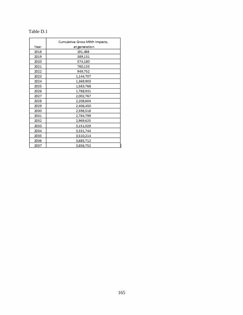
165

Table D.1

166

Please note that the table above reflects the projected impacts for 2018 based on the portfolio

approved in DSM-4 due to the timing of the IRP analysis. Actual results for 2018 were

approximately 233,000 MWh at generation (approximately 215,000 MWh at meter).

Table D.2 provides the MW impacts from the special contracts and demand response programs.

The MW impacts from the selected EE programs are included in the Load Forecasting section.

Table D.2 MW LOAD IMPACTS OF DR PROGRAMS5

Demand Response Program Load Impacts

MW Year PowerShare Power Manager Interruptible Total DR 2018 311 69 197 576 2019 316 76 197 588 2020 324 82 197 603 2021 332 86 197 615 2022 341 90 197 628 2023 349 95 197 640 2024 349 95 197 640 2025 349 95 197 640 2026 349 95 197 640 2027 349 95 197 640 2028 349 95 197 640 2029 349 95 197 640 2030 349 95 197 640 2031 349 95 197 640 2032 349 95 197 640 2033 349 95 197 640 2034 349 95 197 640 2035 349 95 197 640 2036 349 95 197 640 2037 349 95 197 640

5 DR MWs for Power Manager includes MWs from Power Manager, Power Manager Water Heaters, Power Manager for Apartments, and Power Manager for Business.

167

E. EXISTING ENERGY EFFICIENCY PROGRAMS, HISTORICAL PERFORMANCE

Duke Energy Indiana has been aggressive in the planning and implementation of energy efficiency

programs. The forecast of loads provided in Chapter 3 incorporates the effects of these historical

impacts in the baseline forecast, subject to anticipated “roll off” into prevailing codes and

standards.

F. INTEGRATED VOLT-VAR CONTROL (IVVC)

Duke Energy is implementing grid modernization throughout the enterprise with a vision of

creating a sustainable energy future for our customers and our business by being a leader of

innovative approaches that will modernize the grid.

Duke Energy Indiana is reviewing an IVVC project that will better manage the application and

operation of voltage regulators (the Volt) and capacitors (the VAR) on the Duke Energy Indiana

distribution system. In general, the project will optimize the operation of these devices, resulting

in a reduction and “flattening” of the voltage profile across an entire circuit, starting at the

substation and continuing out to the farthest endpoint on that circuit. This flattening of the voltage

profile is accomplished by automating the substation level voltage regulation devices and

capacitors, distribution line capacitors, and distribution line voltage regulators, while integrating

them into a single control system. The control system continuously monitors and operates the

voltage regulators and capacitors in near real time, coordinated control to maintain the optimized

“flat” voltage profile. Once the system is operating with a flat voltage profile across an entire

circuit, the net result is a reduction of system loading.

The deployment of an IVVC program for Duke Energy Indiana is anticipated to take

approximately seven years. This IVVC program is projected to reduce future distribution-only

system peak needs by approximately 0.215% in 2020, 0.38% in 2021, 0.53% in 2022, and 0.7% in

2023 and beyond. While the subject of grid modernization is very broad, only the supply and

demand impacts of the IVVC program is included in the IRP process.

168

1. Avoided Cost for EE Screening

The avoided costs used in screening the EE and DR programs in the Market Potential Study to

determine the Economic Potential were based on information in the New Portfolio Program filing

(Cause No. 43955 – DSM4) made with the Commission. The Company considers this

information to be a trade secret and confidential and competitive information. It will be made

available to appropriate parties for viewing at Duke Energy Indiana offices during normal

business hours upon execution of an appropriate confidentiality agreement or protective

order. Please contact Kelley Karn at (317) 838-2461 for more information.

2. Duke Energy Indiana EE Program Data EE and DR Program data is voluminous, and will be made available to appropriate parties for

viewing at Duke Energy Indiana offices during normal business hours. Please contact Kelley

Karn at (317) 838-2461 for more information.

169

Table D.4 Benefit/Cost Test Components and Equations

BENEFIT/COST TEST MATRIX Benefits:

Participant

Test

Utility Test

Ratepayer Impact

Test

Total Resource

Test

Societal

Test Customer Electric Bill Decrease X Customer Non-electric Bill Decrease X Customer O&M a nd Other Cost Decrease X X X Customer Income Tax Decrease X X Customer Investment Decrease X X X Customer Rebates Received X Utility Revenue Increase X Utility Electric Production Cost Decrease X X X X Utility Generation Capacity Credit X X X X Utility Transmission Capacity Credit X X X X Utility Distribution Capacity Credit X X X X Utility Administrative Cost Decrease X X X X Utility Cap. Administrative Cost Decrease X X X X Non-electric Acquisition Cost Decrease X X Utility Sales Tax Cost Decrease X X X Costs: Customer Electric Bill Increase X Customer Non-electric Bill Increase X X Customer O&M and Other Cost Increase X X X Customer Income Tax Increase X X Customer Capital Investment Increase X X X Utility Revenue Decrease X Utility Electric Production Cost Increase X X X X Utility Generation Capacity Debit X X X X Utility Transmission Capacity Debit X X X X Utility Distribution Capacity Debit X X X X Utility Rebates Paid X X Utility Administrative Cost Increase X X X X Utility Cap. Administrative Cost Increase X X X X Non-electric Acquisition Cost Increase X X Utility Sales Tax Cost Increase X X X

Benefit/Cost Ratio = Total Benefits/Total Costs

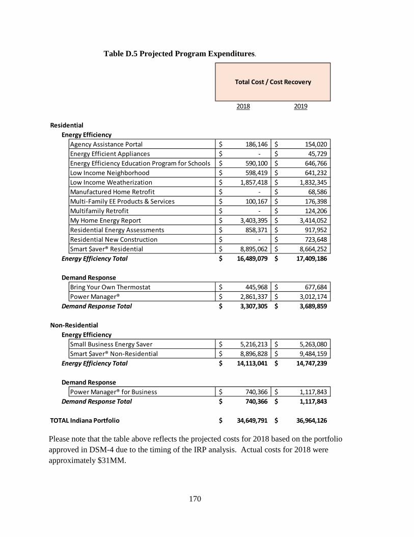
170

Table D.5 Projected Program Expenditures.

Please note that the table above reflects the projected costs for 2018 based on the portfolio approved in DSM-4 due to the timing of the IRP analysis. Actual costs for 2018 were approximately $31MM.

2018 2019

ResidentialEnergy Efficiency

Agency Assistance Portal 186,146$ 154,020$ Energy Efficient Appliances -$ 45,729$ Energy Efficiency Education Program for Schools 590,100$ 646,766$ Low Income Neighborhood 598,419$ 641,232$ Low Income Weatherization 1,857,418$ 1,832,345$ Manufactured Home Retrofit -$ 68,586$ Multi-Family EE Products & Services 100,167$ 176,398$ Multifamily Retrofit -$ 124,206$ My Home Energy Report 3,403,395$ 3,414,052$ Residential Energy Assessments 858,371$ 917,952$ Residential New Construction -$ 723,648$ Smart $aver® Residential 8,895,062$ 8,664,252$

Energy Efficiency Total 16,489,079$ 17,409,186$

Demand ResponseBring Your Own Thermostat 445,968$ 677,684$ Power Manager® 2,861,337$ 3,012,174$

Demand Response Total 3,307,305$ 3,689,859$

Non-ResidentialEnergy Efficiency

Small Business Energy Saver 5,216,213$ 5,263,080$ Smart $aver® Non-Residential 8,896,828$ 9,484,159$

Energy Efficiency Total 14,113,041$ 14,747,239$

Demand ResponseSB Power Manager® for Business 740,366$ 1,117,843$ Demand Response Total 740,366$ 1,117,843$

TOTAL Indiana Portfolio 34,649,791$ 36,964,126$

Total Cost / Cost Recovery

171

The Duke Energy Indiana 2018 Integrated Resource Plan July 1, 2019

Appendix E: Transmission Planning

172

1. TRANSMISSION EXECUTIVE SUMMARY

A. System Description

The Duke Energy Indiana bulk transmission system is comprised of the 345 kilovolt (kV), 230

kV, and 138 kV systems. The Duke Energy Indiana transmission system serves primarily to

deliver bulk power into and/or across Duke Energy Indiana service area. This bulk power is

distributed to numerous substations that supply lower voltage sub-transmission systems and

distribution circuits, or directly to large customer loads. Because of the numerous

interconnections Duke Energy Indiana has with neighboring local balancing areas, the Duke

Energy Indiana transmission system increases electric system reliability and decreases costs to

customer by permitting the exchange of power and energy with other utilities on an emergency

or economic basis.

As of December 2018, Duke Energy Indiana’s wholly and jointly owned share of bulk

transmission included approximately 852 circuit miles of 345 kV lines, 777 of 230 kV, and 1446

of 138 kV. Duke Energy Indiana, Indiana Municipal Power Agency (IMPA), and Wabash Valley

Power Alliance (WVPA) own the Joint Transmission System (JTS) in Indiana. The three co-

owners have rights to use the JTS. Duke Energy Indiana is directly interconnected with seven

other local balancing authorities (American Electric Power, Louisville Gas and Electric Energy,

Ameren, Hoosier Energy, Indianapolis Power and Light, Northern Indiana Public Service

Company, and Vectren) plus Duke Energy Ohio.

B. Electric Transmission Forecast

As a member of MISO, Duke Energy Indiana participates in the MISO planning processes, and

is subject to MISO overview and coordination mechanisms. All of Duke Energy Indiana’s

transmission facilities, including those transmission facilities owned by WVPA and IMPA but

operated and maintained by Duke Energy Indiana, are included in these MISO planning

processes. Additional coordination occurs through a variety of mechanisms, including

ReliabilityFirst Corporation (RFC) and joint meetings with the other entities held as necessary.

173

2. ELECTRIC TRANSMISSION FORECAST

A. General Description

The Duke Energy Indiana bulk transmission system is comprised of 138 kV, 230 kV, and 345 kV

systems. The 345 kV system distributes power from Duke Energy Indiana’s large generating units,

and interconnects the Duke Energy Indiana system with other systems. The 345 kV system is

connected to the 138 kV and 230 kV systems through large transformers at a number of substations

across the system. These 138 kV and 230 kV systems distribute power received through the

transformers and from several smaller generating units, which are connected directly at these

voltage levels. This power is distributed to substations, which supply lower voltage sub-

transmission systems and distribution circuits, or directly to a number of large customer loads.

B. Transmission and Distribution Planning Process

Transmission and distribution (T&D) planning is a complex process which requires the evaluation

of numerous factors to provide meaningful insights into the performance of the system. Duke

Energy Indiana’s distribution system planners gather information concerning actual distribution

substation transformer and line loadings. The loading trend for each transformer is examined, and

a projection of future transformer bank loading is made based on the historic load growth combined

with the distribution planners’ knowledge of load additions within the area. The load growth in a

distribution planning area tends to be somewhat more uncertain and difficult to predict than the

load forecasts made for Duke Energy Indiana as a whole.

Customers’ decisions can dramatically impact the location and timing of future distribution

capacity, and system improvement projects. Because of this uncertainty, distribution development

plans are under continual review to make sure proposed projects remain appropriate for the area’s

needs.

T&D planning generally depends on the specific location of the loads, therefore the effects of co-

generation capacity on T&D planning is location-specific. To the extent that fewer new T&D

resources are required to serve these customers or the local areas in which they reside, Duke

Energy Indiana's T&D planning will reflect this change.

174

Adding new distribution substation capacity to an area typically takes 18 to 24 months. Factors

related to the future customer load, such as local knowledge of growth potential based on zoning,

highway access and surrounding development, can help forecast ultimate distribution system

needs.

Transmission system planners utilize the historical distribution substation transformer bank

loading and trends, combined with the Duke Energy Indiana load forecast and resource plan and

firm service schedules, to develop models of the transmission system. These models are used to

simulate the transmission system performance under a range of credible conditions to ensure that

expected performance meets both North American Electric Reliability Corporation (NERC) and

Duke Energy Indiana planning criteria. Should these simulations indicate that a violation of the

planning criteria occurs, more detailed studies are conducted to determine the severity of the

problem and possible measures to alleviate it.

Duke Energy Indiana’s planning criteria are filed under the FERC Form 715 Part 4. The Company

adheres to any applicable NERC and RFC Reliability Standards, and to its own detailed planning

criteria, which are shown in the following paragraphs. Violations of these criteria would require

expansion of transmission system and/or new or revised operating procedures. Acceptance of

operating procedures is based on engineering judgment with the consideration of the probability

of violation weighed against its consequences and other factors.

Voltage

Bus voltages are screened using the Transmission System Voltage Limits below. These Limits

specify minimum and maximum voltage levels during both normal and contingency conditions.

Emergency Voltage Limits are defined as the upper and lower operating limits of each bus on the

system. Voltage limits are expressed as a percent of nominal voltage. All voltages should be

maintained within the appropriate Emergency voltage limits.

175

Table E.1: Transmission System Voltage Limits

Thermal

The following guidelines shall be used to ensure acceptable thermal loadings:

a) In normal conditions, no facility should exceed its continuous thermal loading capability.

b) For a single contingency, no facility should exceed its emergency loading capability.

Stability

The stability of the Duke Energy Indiana system and neighboring systems must be maintained for

the contingencies specified in the applicable sections of the NERC and RFC Reliability

Standards. Generating units must maintain angular stability under various contingency

situations. Many different contingencies are considered and the selection is dependent on the

location within the transmission system.

Fault Duty

All circuit breakers should be capable of interrupting the maximum fault current duty imposed

on the circuit breaker.

Single Contingencies

The thermal and voltage limits should not be violated for either normal operations or under the

loss of:

a) A single transmission circuit

b) A single transformer

c) A single generating unit

d) A single reactive power source or sink

Nominal Voltage (kV)

Normal Voltage Limits Minimum Maximum

Emergency Voltage Limits Minimum Maximum

345 95% 105% 90% 105% 230 95% 107% 90% 107% 138 95% 105% 90% 105%

176

Severe Contingencies

NERC Reliability Standards include evaluation of extreme (highly improbable) contingency

events causing multiple elements to be removed or cascade out of service. Severe contingencies

are evaluated to determine the impact on the Duke Energy Indiana and interconnected transmission

systems. These evaluations are not intended to be absolute or applied without exception. Other

factors, such as severity of consequences, availability of emergency switching procedures,

probability of occurrence and the cost of remedial action are also considered in the evaluation of

the transmission system.

C. System-Wide Reliability Measure

At the present time, there is no measure of system-wide reliability that covers the entire system

(transmission, distribution, and generation).

D. Evaluation of Adequacy for Load Growth

The transmission system of Duke Energy Indiana is adequate to support load growth and the

expected power transfers over the next ten years if the planned transmission system expansions

are completed as currently scheduled. Duke Energy Indiana’s transmission system can be

significantly affected by the actions of others. In an attempt to evaluate these effects, RFC

develops a series of power flow simulation base cases that reflect the expected transmission system

configuration and expected power transfers. Should actual conditions differ significantly from

those assumed in the base cases, a re-evaluation of the adequacy of the Duke Energy Indiana

transmission system would be required.

E. Economic/Loss Evaluation

As a member of MISO, Duke Energy Indiana actively participates in the MISO Transmission

Expansion Planning (MTEP) assessment and study processes which include economic analysis.

MISO utilizes PROMOD, a commercial production cost model, to evaluate potential economic

benefits of transmission projects or portfolios. Production cost model simulations are performed

with and without each developed transmission project or portfolio. Taking the difference between

these two cases provides the economic benefits associated with each project or portfolio. The

economic benefits include adjusted production cost savings, reduced energy and capacity losses,

177

and reduced congestion cost. Projects that meet initial qualification criteria will be further

evaluated under the appropriate MISO or interregional planning process.

F. Transmission Expansion Plans

The transmission system expansion plans for the Duke Energy Indiana system are developed for

the purpose of meeting the projected future requirements of the transmission system using power

flow analysis. Power flow representations of the Duke Energy Indiana electric transmission

system, which allow computer simulations to determine MW and MVAR flows and the voltages

across the system, are maintained for the peak periods of the current and future years. These power

flow base cases simulate the system under normal conditions with typical generation and no

transmission outages. They are used to determine the general performance of the existing and

planned transmission system under normal conditions.

Contingency cases based on the peak load base cases are studied to determine system performance

for planned and unplanned transmission and generation outages. The results of these studies are

used to determine the need for and timing of additions to the transmission system. As indicated

earlier, Duke Energy Indiana, as a member of the MISO actively participate in the MISO MTEP

assessment and study processes by reviewing the modeling data, providing simulation scenarios,

and reviewing and providing feedback on the results of MTEP assessments and studies. All of

Duke Energy Indiana’s transmission facilities, including those transmission facilities owned by

WVPA and IMPA but operated and maintained by Duke Energy Indiana, are included in these

MISO processes. In addition, MISO reviews Duke Energy Indiana’s proposed plans and makes

comments and suggestions. Ultimately, MISO has responsibility for development of the regional

transmission plan. MTEP 18 assessed the Duke Energy Indiana transmission system for the period

2018 through 2028 with simulations for years 2020, 2023 and 2028. These models were utilized

to simulate both steady state and dynamic performance under a wide variety of credible conditions,

such as Summer Peak, Shoulder Peak, and Light Load, to ensure that expected performance meets

both NERC and Duke Energy Indiana planning criteria.

The MTEP studies provide an indication of system performance under a variety of conditions to

guide the development of a comprehensive expansion plan that meets both reliability and economic

expansion needs. The planning process identifies solutions to reliability issues that arise from the

178

expected dispatch of network resources. These solutions include evaluating alternative costs

between capital expenditures for transmission expansion projects and increased operating

expenses from redispatching network resources or other operational actions.

G. Transmission Project Descriptions

The following planned transmission projects include new substation transformers, transmission

capacitors, transmission circuits, and upgrades of existing circuits and substations.

Sugar Creek to Ameren Kansas 345 kV line consist of construction of 1.5 miles of 345 kV line.

The new line will be routed from the Duke Energy Indiana Sugar Creek Substation to the state line

between Indiana and Illinois state line. The remaining section to will be built by Ameren. This

project will relief congestion for the Kansas area and promote access to renewable generation.

Lafayette South East to Concord Road Junction 138 kV reconductor project. Included in project,

adding a 138 kV breaker in the Lafayette South East Substation ring bus and tapping another line

between Lafayette South and Concord Road. The project will reduce 138 kV line exposure and

reduce outage minutes to Lafayette industrial customers.

The Speed to Jeffersonville 138kV line project enhances the bulk electric supply system serving

the Clarksville Maritime load area. The Clarksville Maritime Center industrial park has port access

off of the Ohio River and by the end of 2019 will be next to a new interstate highway extension

from I265 in Kentucky over the Ohio River to I65 in Indiana. Just east of the Clark Maritime

Center and the interstate extension is a new developing industrial park called River Ridge

Commerce Center. The existing bulk transmission source to the Clark Maritime Center Industrial

Park and River Ridge Commerce Center is provided from a tap off of a 138kV circuit that runs

between Jeffersonville and Gallagher. The reserving source is off of a 138kV circuit that runs

between the Speed substation and the Madison substation. This project will provide for a more

secure and reliable 138kV source line for this load area by creating a new looped bulk system

source line between the Speed substation and the Jeffersonville substation.

179

H. Economic Projects Comments

Duke Energy Indiana continues to stay abreast of MISO expansion criteria and participate in MISO

studies and evaluate transmission projects that provide economic value to Duke Energy Indiana

customers.

I. Short Term Implementation Plan - Planned New Transmission Facilities

Description of Projects

See the tables below for status of previous projects reported as well as a current projects listing.

More detailed descriptions of the current projects can be found in Section 2.G of this Appendix.

Criteria and Objectives for Monitoring Success

Milestones and criteria used to monitor the transmission facilities projects are typical of

construction projects and measured on the following factors:

• Comparison of the actual completion date to the targeted completion date

• Comparison of the actual cost to the budgeted cost

Anticipated Time Frame and Estimated Costs

The cash flows associated with the major new transmission facility projects planned are shown

below.

180

Table E.2: STATUS UPDATES AND CHANGES FROM PREVIOUS REPORT DUKE ENERGY INDIANA TRANSMISSION PROJECTS

CASH FLOWS ($000)*

PROJECT NAME

MILES or MVA

kV

PROGRESS/

COMPLETION DATE

2015 2016 2017

Westpoint 230 kV Switching Station

- 230 12/31/15 Canceled 6-18-2014 (Note 1)

Lafayette 230 kV Sub Breaker Repl with Ring Bus Phase 1

- 230 12/31/2014 Completed 12/31/14

$11 $2652 $0

Table E.3: CURRENT DUKE ENERGY INDIANA MAJOR TRANSMISSION PROJECTS

CASH FLOWS ($000)*

PROJECT NAME

MILES or MVA

kV

PROGRESS/

COMPLETION DATE

2018 2019 2020

Sugar Creek to Ameren Kansas

1.5 345 6/5/2019 $9,348 $5,986 $0

Laf SE Conc Rd. Jct 138kV Line (Note 2)

3.6 138 1/15/2020 $3,205 $116 $0

Speed to Jeffersonville 138 kV line (Note 2)

2.5 138 3/26/2019 $1,861 $3,998 $923

*Excluding AFUDC

Anticipated Project Milestones – update as needed

The completion of these projects, by their planned in-service dates and costs, are the project milestones. Individual project specific notes from the above tables are given as follows: Note 1 – Wind developer requested project to be canceled. Note 2 – Project will be partially funded by IMPA as part of their obligations as joint owner of the Duke Energy Indiana transmission system.

181

The Duke Energy Indiana 2018 Integrated Resource Plan July 1, 2019

Appendix F: Environmental Compliance

182

ENVIRONMENTAL COMPLIANCE

A. INTRODUCTION

The environmental compliance planning process develops an integrated resource/compliance plan

meeting future resource needs and environmental requirements in a reliable and economic manner.

Compliance planning associated with existing laws and regulations is discussed in Section B.

Risks associated with anticipated and potential changes to environmental regulations are discussed

in Section C. B. COMPLIANCE PLANNING – EXISTING LAWS AND REGULATIONS

1. Ozone National Ambient Air Quality Standards (“NAAQS”)

On October 1, 2015, EPA finalized a rule lowering the ozone standard from 75 to 70 ppb. The

EPA finalized attainment designations in 2017, based on actual 2014-2016 ozone air quality

data. EPA designated several Indiana counties as non-attainment including Lake and Porter

Counties (Chicago area), and Clark and Floyd Counties (Louisville area). These counties were

all classified as “marginal” non-attainment, which does not require Indiana to adopt any further

emission controls at facilities in the affected counties provided that the areas achieve

attainment during the first planning period (by 2021). Indiana filed a Good Neighbor plan on

November 2, 2018 which addresses potential significant impact from Indiana sources on

downwind areas in other states that are non-attainment for the 2015 ozone standard. No further

requirements are anticipated at this time.

2. Sulfur Dioxide Ambient Air Quality Standard

On June 22, 2010, EPA established a 75 ppb 1-hour SO2 NAAQS and revoked the annual and

24-hour SO2 standards. EPA finalized initial nonattainment area designations in July 2013.

The area around the Wabash River Station was designated as a nonattainment area. The

Indiana Department of Environmental Management (“IDEM”) submitted a state

implementation plan to EPA on October 2, 2015 that included SO2 emission limits for Wabash

River starting January 1, 2017. Wabash River Units 2-5 were retired in April 2016 in response

to the EPA’s Mercury and Air Toxics Standards (“MATS”) rule. Wabash River Unit 6 was

183

also retired, after a decision not to switch fuels to natural gas, also in response to the MATS

rule. EPA has proposed to redesignate Vigo county to attainment in the May 3, 2019 Federal

Register. All other areas of Indiana where Duke Energy Indiana facilities are located have been

classified as attaining the SO2 NAAQS, and no further SO2 controls or restrictions are

anticipated at these facilities as a result of the SO2 NAAQS.

3. Interstate Transport – Ozone

Phase I of the Cross State Air Pollution Rule (“CSAPR”) took effect on January 1, 2015 and

Phase II of CSAPR took effect on January 1, 2017 for the annual NOx and SO2 programs. EPA

promulgated a “CSAPR Update Rule” in September 2016 which set a more stringent cap on

ozone season NOx emissions, and those more stringent requirements became effective May 1,

2017. The additional reductions required have been achieved through enhanced utilization of

Selective Catalytic Reduction (“SCR”) systems installed at Cayuga and Gibson Stations. For

Cayuga Units 1&2, this enhanced utilization includes operating the SCRs with ammonia

injection during the ozone season to control NOx. Those SCR systems were installed to

promote oxidation and capture of mercury to meet MATS requirements, which does not require

ammonia injection.

On November 16, 2016, the State of Maryland submitted a petition to the EPA under

Section 126 of the Clean Air Act (“CAA”), requesting that EPA impose stringent, short-term

NOx emissions limits on a number of electric utility units that Maryland claimed were having

a significant impact on ozone attainment in Maryland. The sources listed in the petition

included Gibson Unit 3 and Unit 5. EPA formally denied the petition on October 15, 2018,

but the Maryland has filed litigation to appeal EPA’s decision. Duke Energy Indiana has filed

with the Court as an intervenor in support of EPA’s determination. On March 12, 2018, the

State of New York filed a similar Section 126 petition, which alleged that sources including

all of the units at Cayuga, Edwardsport, Gallagher and Gibson Stations were significantly

impacting ozone attainment in New York. On May 20, 2019, EPA published a proposal for

comment that it intended to deny the New York petition. It is possible that New York would

likewise challenge EPA in court if a final decision is made to deny the New York petition. If

either of these Section 126 petitions were granted, Duke Energy Indiana would be required to

comply with the more stringent limits within three months of a final decision, or up to three

184

years if EPA allowed for extensions provided under the CAA. Duke Energy Indiana would

need to evaluate enhancements to existing NOx control systems on any affected units at

Cayuga, Gallagher, and Gibson Stations to determine what additional steps, including potential

operating restrictions, would be required to meet the limits. No impact would be expected at

Edwardsport because of the inherently low emissions rate from those units.

4. MATS

On June 29, 2015 the Supreme Court found that EPA should have considered costs as part of

its determination of whether the regulation of hazardous air pollutants (“HAPs”) from power

plants was appropriate and necessary, and remanded the case to the D.C. Circuit Court for

further proceedings. Despite the Supreme Court’s decision, the MATS rule remains in effect

pending further action by the D.C. Circuit, meaning that all affected sources must continue to

meet the rule requirements. Duke Energy Indiana cannot predict the outcome of the court

proceedings or how it might affect the MATS requirements. However, Duke Energy Indiana’s

coal fired units are complying with all requirements of the MATS rule.

In February 2019, EPA proposed several actions related to the MATS Rule. In response

to the ongoing litigation of the MATS rule, EPA proposed to revoke its 2016 Supplemental

Finding which addressed the Supreme Court’s remand; however, it also proposed to keep the

existing MATS rule in place. EPA also proposed a combined Residual Risk and Technology

Review (“RTR”), which is required within 8 years of adopting a standard (such as MATS)

under Section 112 of the Clean Air Act. In the RTR, EPA proposed to find that any residual

risks are below any threshold of regulatory concern and that there are no developments in

practices, processes, and control technologies that warrant revisions of the current MATS

standards and no additional restrictions are anticipated at this time.

5. Steam Electric Effluent Limitation Guidelines

EPA signed the final revisions to the Steam Electric Effluent Limitations Guidelines (“ELG”)

on September 30, 2015. The new limitations are incorporated into a station’s National Pollutant

Discharge Elimination System (“NPDES”) permit upon renewal. The rule requires the new

limitations for some waste streams to apply based on a date determined by the permitting

authority that is as soon as possible beginning November 1, 2018 but no later than December

185

31, 2023. For flue gas desulfurization (“FGD”) and Bottom Ash Transport Water (“BATW”),

the EPA issued a final rule on September 18, 2017 to postpone the initial deadline to November

1, 2020, but no later than December 31, 2023. Furthermore, Best Available Technology

(“BAT”) for the FGD and BATW wastestreams will be subject to a proposed rulemaking

during 2019 that is scheduled to be finalized during 2020. For coal combustion residuals

(“CCR”) leachate, the limits are effective immediately upon issuance of the permit after the

effective date of the rule; however, this was vacated and remanded to the EPA for further

consideration on April 12, 2019 by the Fifth Circuit United States Court of Appeals. The

compliance dates determined by IDEM will be dependent on the site specific-modifications

necessary. Duke Energy Indiana has installed wastewater treatment that is believed to be

compliant with the rule, as appropriate for a specific DEI facility, including dry fly and bottom

ash systems, and plant process wastewater management systems.

6. Clean Water Act Section 316(a) and 316(b)

The latest 316(b) rule revision was published in the Federal Register on August 15, 2014, with

an effective date of October 14, 2014. The final regulation establishes aquatic protection

requirements at existing facilities and new on-site generation that withdraw 2 million gallons

per day (MGD) or more from rivers, streams, lakes, reservoirs, estuaries, oceans, or other U.S.

waters, utilizes at least 25% of the water withdrawn for cooling purposes, and has a NPDES

discharge permit.

The rule requires facilities with a NPDES permit expiring after July 14, 2018 to submit all

necessary 316(b) reports with the renewal application. For facilities with a NPDES permit

expiring prior to July 14, 2018 or are in the renewal process, the state permitting agency is

allowed to establish an alternate submittal schedule. Duke Energy Indiana submitted 316(b)

study reports for Gibson during 2019. The Gallagher reports will be submitted no later than

July 30, 2019 and the Cayuga reports will be submitted no later than April 30, 2020. Any

required intake modification would be anticipated to occur during the 2021 to 2023 timeframe,

depending on the NPDES compliance schedule developed by IDEM. At this time, we believe

that DEI facilities are compliant with the 316(b) rule; however, installation of new fish friendly

traveling screens (“modified Ristroph”) may be required at Cayuga.

186

C. ENVIRONMENTAL RISK/REGULATORY IMPACTS

Several environmental risks/regulatory changes can affect Duke Energy Indiana in the future. The

Company closely monitors these changes and develops responses when necessary.

1. Particulate Matter NAAQS (PM 2.5)

On December 14, 2012, EPA finalized a rule lowering the annual PM2.5 standard from 15 to

12 ug/m3 and retaining the 35 ug/m3 daily PM2.5 standard. The EPA finalized area designations

for the standard in early 2015. No areas in the Company’s service territory were designated as

nonattainment areas for the revised standard. To date, neither the annual nor the daily PM2.5

standard has directly driven emission reduction requirements at Duke Energy Indiana facilities.

The reduction in SO2 and NOx emissions to address the PM2.5 standards has been achieved

through CAIR and CSAPR, each developed to address interstate transport. At this time, there

is no indication that the revised PM2.5 standard will result in EPA developing a new PM2.5

interstate transport rule.

2. Coal Combustion Residuals

On April 17, 2015 EPA published its final rule for the disposal of CCRs. The rule regulates

CCRs as a non-hazardous waste under Subtitle D of the Resource Conservation Recovery Act

(“RCRA”). This is the first federal regulation of CCRs. The effective date of the rule was

October 19, 2015, starting with the obligation to comply with the operating requirements.

The rule is applicable to all new and existing landfills and surface impoundments used to

store or dispose of CCRs if they are located at a power plant actively generating electricity,

regardless of fuel source being used. In addition to surface impoundments that are actively

receiving CCRs, the rule applies to CCRs surface impoundments no longer receiving CCRs if

they contain CCRs and liquids and are located at a power plant that is currently producing

electricity. These impoundments are defined as inactive impoundments. The rule does not

apply to inactive landfills. The rule will result in the closure of all existing surface

impoundments used to store or dispose of CCRs and treat non-CCR wastewaters. The closure

of surface impoundments lead to dry handling of fly ash and bottom ash and the need for

additional landfill capacity. It has also result in a need for alternative wastewater treatment for

187

the non-CCR wastewaters in smaller lined ponds. The regulatory deadlines that have factored

into the closure of surface impoundments include non-compliance with structural integrity

standards (April 2017), exceedance of ground water protection standards (April 2018), or

failure to demonstrate compliance with location restrictions (April 2019). Duke Energy

Indiana filed with the IDEM in December 2016 closure plans to either close in place or

excavate impoundments at all facilities. At this time IDEM has not approved any of our

proposed closure plans.

3. Greenhouse Gas Regulation In June 2019, EPA finalized the Affordable Clean Energy (“ACE”) rule to replace the previous

Clean Power Plan. The ACE rule will require CO2 emissions reductions from existing coal-

fired electric generating units by requiring states to develop implementation plans based on

efficiency improvements that can be adopted “inside the fence” at existing power plants. The

EPA Administrator signed the final ACE rule on June 19, 2019. The rule will become effective

after it is published in the Federal Register. The final ACE lists seven measures for efficiency

improvements that states should consider for application at individual units6. States will have

three years to develop implementation plans. The implementation plans must include

enforceable emissions performance standards for each coal-fired unit, in terms of pounds of

CO2 per MWH of electricity produced. Compliance will be required within two years after

state plan approval by EPA, or roughly in the 2024-2025 timeframe.

Duke Energy Indiana’s Gibson and Cayuga coal-fired units have already installed the most

significant of the measures identified in the final ACE rule. That includes stream turbine blade

path upgrades, and variable frequency drives on induced draft fans. Gibson Station also has

operating neural networks on its units. The economizers on the Gibson and Cayuga units have

also already been replaced, having been optimized for heat recovery while balancing the

required gas temperatures for proper operation of SCR catalyst for NOx control. The

remaining measures are generally smaller in scope and cost to implement.

6The seven measures EPA lists in the ACE rule are neural networks/intelligent sootblowers; boiler feed pump upgrades; air heater and duct leakage control; variable frequency drives; steam turbine blade path upgrades; redesign/replace economizer; and improved operating and maintenance practices.

188

On August 3, 2015, EPA finalized a rule that established CO2 emission standards for new,

modified, and reconstructed fossil-fuel power plants, the Greenhouse Gas New Source

Performance Standards (“NSPS”). This final rule would have prevented Duke Energy Indiana

from developing any new coal-fired power plants that are not equipped with carbon capture

and storage technology. On December 6, 2018, EPA proposed to revise the CO2 emissions

standards for new-modified, and reconstructed fossil fuel-fired power plants. This proposal

would replace the 2015 rule with one that requires new large coal units to meet an emission

rate reflective of supercritical operation (1,900 lb CO2/MWhr).

D. ENVIRONMENTAL COMPLIANCE PLAN

The current modeling analysis primarily focused on compliance with the 316(b) rule requirements.

For CCR and ELG compliance, conversion to dry ash handling and waste water treatment projects

are already complete; ongoing future landfill construction costs were included in the analysis. For

316(b) compliance, based on site-specific considerations, standard mesh and fish friendly screens

and fish return systems were assumed. The Engineering Screening Model was used to provide the

cost of these technologies.

In summary, for purposes of this IRP, the suite of non-carbon related future environmental

regulations and general requirements modeled included:

• CCR Rule, and ELG revisions

o Ongoing Future Landfill construction costs

• 316(b) Intake Structure Rule

o Aquatic impingement and entrainment studies

o Intake structure and traveling screen upgrade costs

o Cooling tower installations were assumed to be mandated for coastal and estuarial

units, but this assumption only impacted the development of fundamental forecast

inputs as none of Duke Energy Indiana’s assets meets these criteria

o The unit compliance timeframes were based off of each facility’s NPDES permit

renewal schedule per the proposed rule.

The balance of all assumptions for the compliance analysis were reviewed and updated where

necessary to coincide with the other assumptions used for the development of this IRP.

189

1. Modeling Assumptions

For this analysis, Duke Energy Indiana utilized a similar analytical modeling process to past

compliance planning activities. Forecasts used in planning included fuel price forecasts from

IHS Markit, ABB’s PROMOD model for forecasting future MISO power prices, and

observable market curves and extrapolation for emission allowance prices. Duke Energy

Indiana’s internal Engineering Screening Model provided input to the modeling process as

described in paragraph 2 below.

2. Engineering Screening Model

Historically, Duke Energy Indiana’s in-house Engineering Environmental Compliance

Planning and Screening Model (“Engineering Screening Model”) has been used to pre-screen

environmental compliance options. As some generating units have already been committed to

retirement and others are already well controlled, no specific screening activity was performed

for this IRP. The Engineering Screening Model was used to support this IRP by organizing

modeling information and providing some modeling characteristic data for future compliance

costs to the System Optimizer and Planning and Risk models. The model is considered

proprietary confidential and competitive information by Duke Energy Indiana.

3. System Optimizer / Planning and Risk Results

The modeled costs associated with CCR, ELG, and 316(b) were passed to the System

Optimizer and Planning and Risk models from the Engineering Screening Model. The costs

associated with operations utilizing these emissions controls were reflected in unit operating

costs and considered in the integration step of this IRP in conjunction with energy efficiency

and various supply-side alternatives.

E. EMISSION ALLOWANCE MANAGEMENT

Table F.1 shows the base number of SO2 allowances allotted by the US EPA for affected units on

the Duke Energy Indiana system for the CSAPR 2019 through 2022 control periods. Tables F.2

and F.3 show the base number of Seasonal and Annual NOx allowances, respectively, allotted by

the US EPA for affected units on the Duke Energy Indiana system for the CSAPR 2019 through

2022 control periods. Beginning with control period 2023, the state of Indiana has an approved

190

State Implementation Plan to administer the CSAPR program. As a result, allowances that Duke

Energy Indiana receives beginning in 2023 may differ somewhat from the allocations that would

have been received under the federal program. The change to allocations is anticipated to be minor

and have minimal impact to compliance strategies.

The emission allowance markets can impact compliance strategies. The projected allowance

market price is a basis against which the costs of compliance options are compared to determine

whether the options are economic (i.e., a “market-based” compliance planning process). The

market pricing for annual SO2 and NOx allowances has seen a significant drop since 2015 (when

the CSAPR program went into effect) due to substantial decreases in regional annual SO2 and NOx

emissions, resulting in low demand for allowances. Those emissions decreases have been driven

largely by retirement of many older, uncontrolled coal-fired units and enhanced operation of

controls on operating coal-fired units in response to the MATS rule. This causes low projected

emission allowance prices for annual SO2 and NOx, typically below the variable cost of control.

Therefore, these markets are not playing a significant role in the environmental compliance

strategy at this time. There remains a demand for ozone season NOx allowances due to additional

limitations on NOx emissions as a result of the 2016 revised CSAPR ozone season rule. However,

even considering the higher cost of ozone season allowance as compared to annual NOx

allowances, the pricing of allowances is still typically below the variable cost of control and is not

a significant factor in longer term environmental compliance strategy. Allowance pricing for

ozone season NOx does play into shorter-term decisions relative to dispatch and short -term

operations and maintenance costs.

Duke Energy Indiana has maintained an interdepartmental group to perform SO2 and NOx

emission allowance management. Duke Energy Indiana manages emissions risk by utilizing a

mixture of purchasing or selling allowances, installing equipment and, when applicable,

purchasing power. The most economic decision is dependent upon the current and forecasted

market price of allowances, the cost and lead-time to install control equipment, and the current and

forecasted market price of power. These factors will be reviewed as the markets change and the

most economic emission compliance strategy will be employed.

191

Table F.1: SO2 Allowances (tons) Allocated to Duke Energy Indiana Units

Station Unit Percent Ownership 2019 2020 2021 2022Cayuga 1 100 4084 4084 4084 4084Cayuga 2 100 4027 4027 4027 4027Edwardsport 6-1 100 1 0 0 0Edwardsport 7-1 100 139 0 0 0Edwardsport 7-2 100 119 0 0 0Edwardsport 8-1 100 143 0 0 0R Gallagher 2 100 948 948 948 948R Gallagher 4 100 907 907 907 907Gibson 1 100 5694 5694 5694 5694Gibson 2 100 5624 5624 5624 5624Gibson 3 100 6082 6082 6082 6082Gibson 4 100 5615 5615 5615 5615Gibson 5 50.05 4825 4825 4825 4825Wabash River Gen Station 2 100 751 751 0 0Wabash River Gen Station 3 100 727 727 0 0Wabash River Gen Station 4 100 840 840 0 0Wabash River Gen Station 5 100 770 770 0 0Wabash River Gen Station 6 100 2857 2857 2857 2857

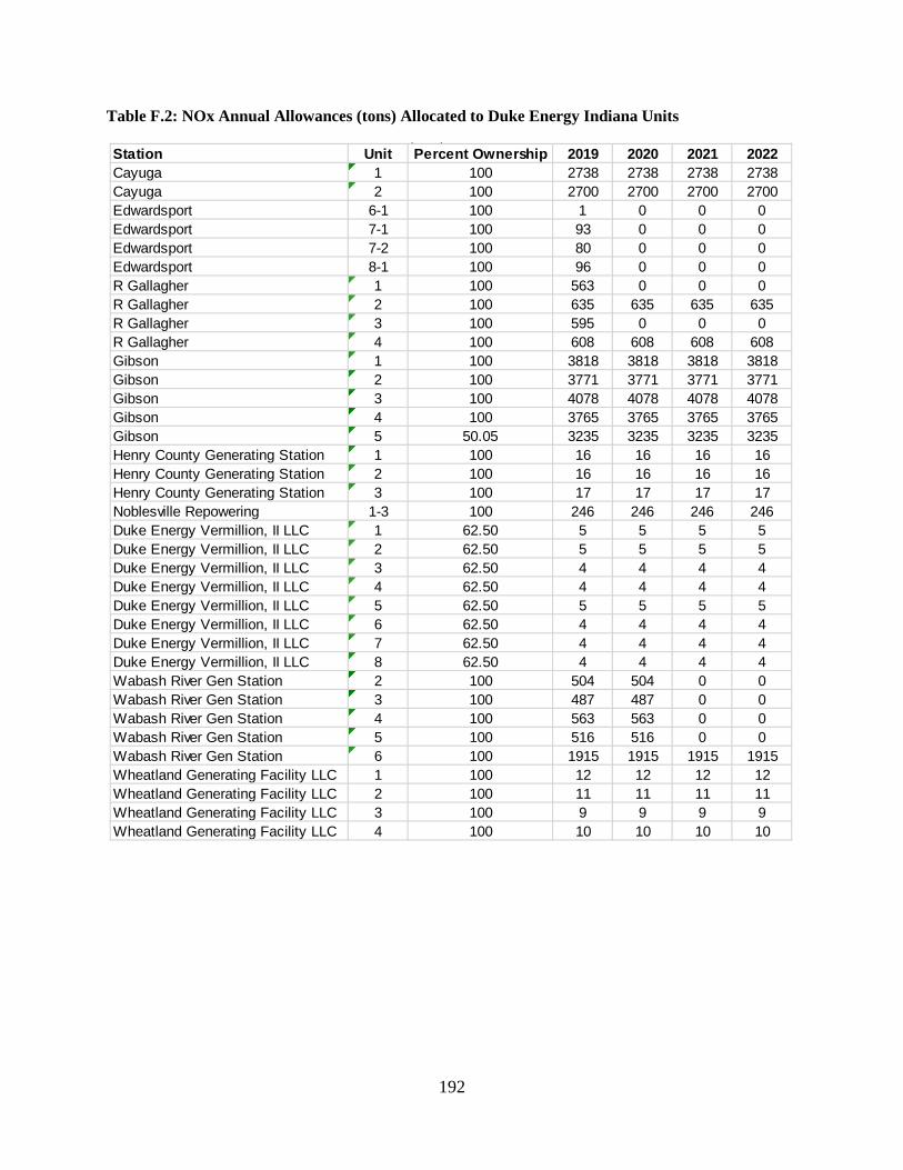
192

Table F.2: NOx Annual Allowances (tons) Allocated to Duke Energy Indiana Units

Station Unit Percent Ownership 2019 2020 2021 2022Cayuga 1 100 2738 2738 2738 2738Cayuga 2 100 2700 2700 2700 2700Edwardsport 6-1 100 1 0 0 0Edwardsport 7-1 100 93 0 0 0Edwardsport 7-2 100 80 0 0 0Edwardsport 8-1 100 96 0 0 0R Gallagher 1 100 563 0 0 0R Gallagher 2 100 635 635 635 635R Gallagher 3 100 595 0 0 0R Gallagher 4 100 608 608 608 608Gibson 1 100 3818 3818 3818 3818Gibson 2 100 3771 3771 3771 3771Gibson 3 100 4078 4078 4078 4078Gibson 4 100 3765 3765 3765 3765Gibson 5 50.05 3235 3235 3235 3235Henry County Generating Station 1 100 16 16 16 16Henry County Generating Station 2 100 16 16 16 16Henry County Generating Station 3 100 17 17 17 17Noblesville Repowering 1-3 100 246 246 246 246Duke Energy Vermillion, II LLC 1 62.50 5 5 5 5Duke Energy Vermillion, II LLC 2 62.50 5 5 5 5Duke Energy Vermillion, II LLC 3 62.50 4 4 4 4Duke Energy Vermillion, II LLC 4 62.50 4 4 4 4Duke Energy Vermillion, II LLC 5 62.50 5 5 5 5Duke Energy Vermillion, II LLC 6 62.50 4 4 4 4Duke Energy Vermillion, II LLC 7 62.50 4 4 4 4Duke Energy Vermillion, II LLC 8 62.50 4 4 4 4Wabash River Gen Station 2 100 504 504 0 0Wabash River Gen Station 3 100 487 487 0 0Wabash River Gen Station 4 100 563 563 0 0Wabash River Gen Station 5 100 516 516 0 0Wabash River Gen Station 6 100 1915 1915 1915 1915Wheatland Generating Facility LLC 1 100 12 12 12 12Wheatland Generating Facility LLC 2 100 11 11 11 11Wheatland Generating Facility LLC 3 100 9 9 9 9Wheatland Generating Facility LLC 4 100 10 10 10 10

( )

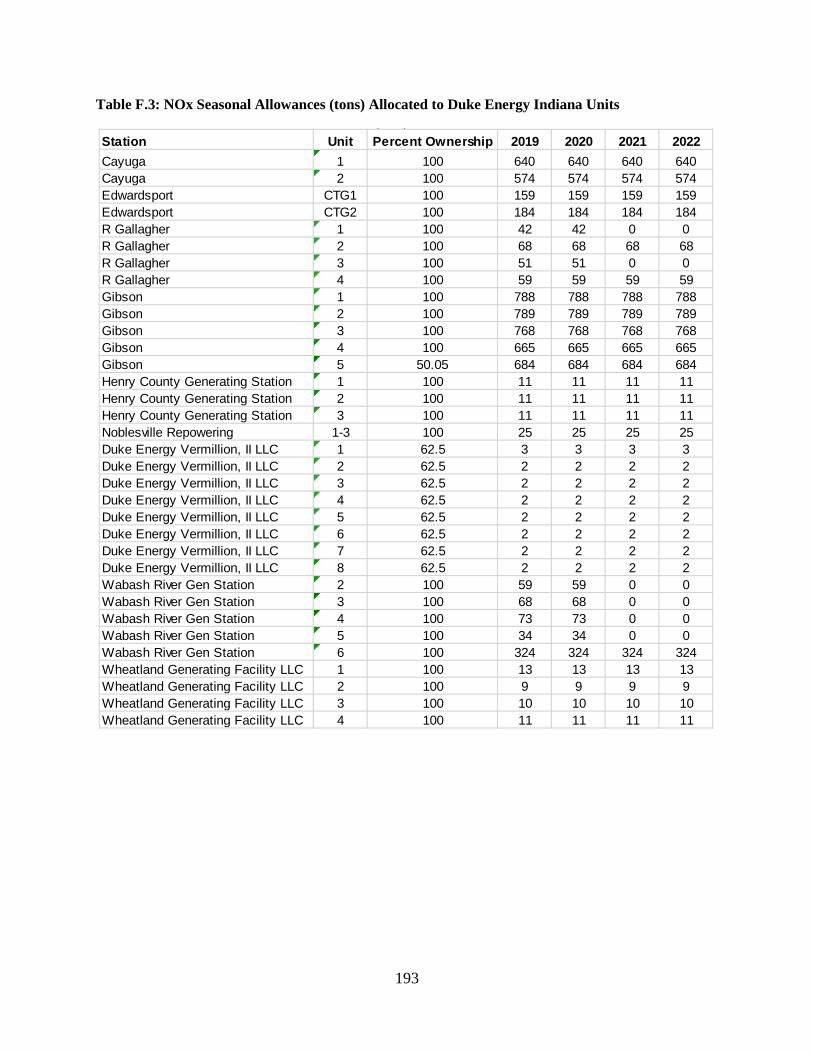
193

Table F.3: NOx Seasonal Allowances (tons) Allocated to Duke Energy Indiana Units

Station Unit Percent Ownership 2019 2020 2021 2022Cayuga 1 100 640 640 640 640Cayuga 2 100 574 574 574 574Edwardsport CTG1 100 159 159 159 159Edwardsport CTG2 100 184 184 184 184R Gallagher 1 100 42 42 0 0R Gallagher 2 100 68 68 68 68R Gallagher 3 100 51 51 0 0R Gallagher 4 100 59 59 59 59Gibson 1 100 788 788 788 788Gibson 2 100 789 789 789 789Gibson 3 100 768 768 768 768Gibson 4 100 665 665 665 665Gibson 5 50.05 684 684 684 684Henry County Generating Station 1 100 11 11 11 11Henry County Generating Station 2 100 11 11 11 11Henry County Generating Station 3 100 11 11 11 11Noblesville Repowering 1-3 100 25 25 25 25Duke Energy Vermillion, II LLC 1 62.5 3 3 3 3Duke Energy Vermillion, II LLC 2 62.5 2 2 2 2Duke Energy Vermillion, II LLC 3 62.5 2 2 2 2Duke Energy Vermillion, II LLC 4 62.5 2 2 2 2Duke Energy Vermillion, II LLC 5 62.5 2 2 2 2Duke Energy Vermillion, II LLC 6 62.5 2 2 2 2Duke Energy Vermillion, II LLC 7 62.5 2 2 2 2Duke Energy Vermillion, II LLC 8 62.5 2 2 2 2Wabash River Gen Station 2 100 59 59 0 0Wabash River Gen Station 3 100 68 68 0 0Wabash River Gen Station 4 100 73 73 0 0Wabash River Gen Station 5 100 34 34 0 0Wabash River Gen Station 6 100 324 324 324 324Wheatland Generating Facility LLC 1 100 13 13 13 13Wheatland Generating Facility LLC 2 100 9 9 9 9Wheatland Generating Facility LLC 3 100 10 10 10 10Wheatland Generating Facility LLC 4 100 11 11 11 11

( )

194

The Duke Energy Indiana 2018 Integrated Resource Plan July 1, 2019

Appendix G: Cross Reference to Proposed Rule

195

170 IAC 4-7 (Proposed 10/6/17) Location in Duke Energy Indiana 2018 IRP Document Regulatory Requirement

Section 0.5 - Purpose and applicability No Response Required Section 1 - Definitions No Response Required Section 2. - Integrated resource plan submission No Response Required

Section 2.1 - Confidentiality No Response Required Section 2.2 - Public comments and director's reports No Response Required Section 2.3 - Resource adequacy assessment No Response Required Section 2.5 - Effects of integrated resource plans in docketed proceedings No Response Required Section 2.6 - Public advisory process No Response Required Section 2.7 - Contemporary issues technical conference No Response Required Section 3. - Waiver or variance requests No Response Required Section 4. - Integrated resource plan contents (1) Twenty-year forecast Section IV

(2) Analysis of historical and forecasted peak demand and energy usage

Section III.A; Section IV.A; Appendix B

(3) Alternative forecasts of peak demand and Section IV; Appendix B energy usage (4) Description of existing resources Section III.B (5) Process for selecting possible future Section II resources (6) Description of possible future resources Section V.A; Appendix C (7) Screening analysis and summary table Section V.A; Appendix C (8) Candidate resource portfolios Section V (9) Preferred resource portfolio Section I; Section V.D; Section VI (10) Short-term action plan Section I; Section VI.B (11) Inputs, methods, and definitions for load forecasts Section II; Section IV

(12) Data sets and sources for load forecasts Appendix B (13) Efforts to develop a database of electricity Appendix B; Appendix D consumption patterns (14) Suggested methods for developing database in (13) No Response Required

(15) Schedule for customer surveys Section II.A (16) Usage of AMI data Section VI (17) Contemporary issues designated None designated

196

(18) Distributed generation Appendix B (19) Model structure and applicability Section II.B (20) Fuel inventory and procurement planning Section II.A (21) Emission allowance inventory and Appendix F procurement planning (22) Generation expansion planning criteria Section II.D; Section V.A (23) Consideration of compliance costs Section IV; Appendix F (24) Resource planning objectives Section II.D; Section V.A (25) Base case scenario Section IV.A (26) Alternative scenarios Section IV (27) Description of power flow models and transmission Appendix E

planning criteria (28) List and description of methods Section II

(29) Avoided cost calculation

The avoided cost is scenario specific

and voluminous. It can be obtained

contact Kelley Karn at (317) 838-2461

for more information.

(30) Summary of public advisory process Volume 2

(31) Assessment of resources considered Section II; Section V; Appendix C; Appendix D

Section 5. - Energy and demand forecasts (a)(1) Historical load shapes Section III.A; Appendix B (a)(2) Disaggregation of data Section III.A; Appendix B (a)(3) Actual and weather-normalized levels Section III.A; Appendix B (a)(4) Methods to weather-normalize Appendix B (a)(5) 20-year energy and demand forecasts Section IV; Appendix B (a)(6) 10-year historical analysis Section III.A; Appendix B (a)(7) Impact of historical DSM programs on Appendix B load forecast (a)(8) Justification for forecast methodology Appendix B (a)(9) Potential improvements for forecasting Appendix B (a)(10) Data sources for historical analysis Appendix B (b)(1) Alternative forecasts - high Section IV; Appendix B (b)(2) Alternative forecasts - low Section IV; Appendix B (b)(3) Alternative forecasts - most probable Section IV; Appendix B (c) Suggested inputs for most probable forecast No Response Required Section 6. - Description of available resources (a)(1) Net and gross dependable generating Section V.A

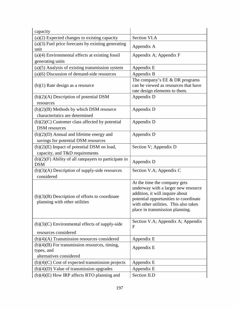
197

capacity (a)(2) Expected changes to existing capacity Section VI.A (a)(3) Fuel price forecasts by existing generating unit Appendix A

(a)(4) Environmental effects at existing fossil Appendix A; Appendix F generating units (a)(5) Analysis of existing transmission system Appendix E (a)(6) Discussion of demand-side resources Appendix B

(b)(1) Rate design as a resource The company’s EE & DR programs can be viewed as resources that have rate design elements to them.

(b)(2)(A) Description of potential DSM Appendix D resources (b)(2)(B) Methods by which DSM resource Appendix D characteristics are determined (b)(2)(C) Customer class affected by potential Appendix D DSM resources (b)(2)(D) Annual and lifetime energy and Appendix D savings for potential DSM resources (b)(2)(E) Impact of potential DSM on load, Section V; Appendix D capacity, and T&D requirements (b)(2)(F) Ability of all ratepayers to participate in DSM Appendix D

(b)(3)(A) Description of supply-side resources Section V.A; Appendix C considered

(b)(3)(B) Description of efforts to coordinate planning with other utilities

At the time the company gets underway with a larger new resource addition, it will inquire about potential opportunities to coordinate with other utilities. This also takes place in transmission planning.

(b)(3)(C) Environmental effects of supply-side Section V.A; Appendix A; Appendix F

resources considered (b)(4)(A) Transmission resources considered Appendix E (b)(4)(B) For transmission resources, timing, types, and Appendix E

alternatives considered (b)(4)(C) Cost of expected transmission projects Appendix E (b)(4)(D) Value of transmission upgrades Appendix E (b)(4)(E) How IRP affects RTO planning and Section II.D

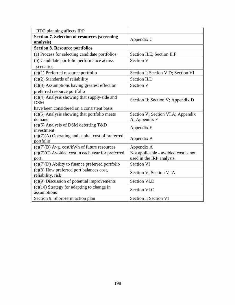
198

RTO planning affects IRP Section 7. Selection of resources (screening analysis) Appendix C

Section 8. Resource portfolios (a) Process for selecting candidate portfolios Section II.E; Section II.F (b) Candidate portfolio performance across Section V scenarios (c)(1) Preferred resource portfolio Section I; Section V.D; Section VI (c)(2) Standards of reliability Section II.D (c)(3) Assumptions having greatest effect on Section V preferred resource portfolio (c)(4) Analysis showing that supply-side and DSM Section II; Section V; Appendix D

have been considered on a consistent basis (c)(5) Analysis showing that portfolio meets demand

Section V; Section VI.A; Appendix A; Appendix F

(c)(6) Analysis of DSM deferring T&D investment Appendix E

(c)(7)(A) Operating and capital cost of preferred portfolio Appendix A

(c)(7)(B) Avg. cost/kWh of future resources Appendix A (c)(7)(C) Avoided cost in each year for preferred port.

Not applicable - avoided cost is not used in the IRP analysis

(c)(7)(D) Ability to finance preferred portfolio Section VI (c)(8) How preferred port balances cost, reliability, risk Section V; Section VI.A

(c)(9) Discussion of potential improvements Section VI.D (c)(10) Strategy for adapting to change in assumptions Section VI.C

Section 9. Short-term action plan Section I; Section VI