The DTW-based representation space for seismic pattern...

Computers & Geosciences 85 (2015) 86–95

Contents lists available at ScienceDirect

Computers & Geosciences

http://d0098-30

n CorrE-m

pacastrojmakari

journal homepage: www.elsevier.com/locate/cageo

The DTW-based representation space for seismic pattern classification

Mauricio Orozco-Alzate a,n, Paola Alexandra Castro-Cabrera a, Manuele Bicego b,John Makario Londoño-Bonilla c

a Universidad Nacional de Colombia, Sede Manizales, Departamento de Informática y Computación, km 7 vía al Magdalena, Manizales 170003, Colombiab Università degli Studi di Verona, Dipartimento di Informatica, Ca' Vignal 2, Strada le Grazie 15, Verona 37134, Italyc Servicio Geológico Colombiano, Observatorio Vulcanológico y Sismológico de Manizales, Av. 12 de Octubre No. 15 – 47, Manizales 170001, Colombia

a r t i c l e i n f o

Article history:Received 9 September 2014Received in revised form14 April 2015Accepted 14 June 2015Available online 17 June 2015

Keywords:ClassificationDissimilarity spaceDynamic time warpingSeismic patternsVolcano monitoring

x.doi.org/10.1016/j.cageo.2015.06.00704/& 2015 Elsevier Ltd. All rights reserved.

esponding author.ail addresses: [email protected] (M. [email protected] (P.A. Castro-Cabrera), [email protected] (J.M. Londoño-Bonilla).

a b s t r a c t

Distinguishing among the different seismic volcanic patterns is still one of the most important and labor-intensive tasks for volcano monitoring. This task could be lightened and made free from subjective biasby using automatic classification techniques. In this context, a core but often overlooked issue is thechoice of an appropriate representation of the data to be classified. Recently, it has been suggested thatusing a relative representation (i.e. proximities, namely dissimilarities on pairs of objects) instead of anabsolute one (i.e. features, namely measurements on single objects) is advantageous to exploit the re-lational information contained in the dissimilarities to derive highly discriminant vector spaces, whereany classifier can be used. According to that motivation, this paper investigates the suitability of a dy-namic time warping (DTW) dissimilarity-based vector representation for the classification of seismicpatterns. Results show the usefulness of such a representation in the seismic pattern classification sce-nario, including analyses of potential benefits from recent advances in the dissimilarity-based paradigmsuch as the proper selection of representation sets and the combination of different dissimilarity re-presentations that might be available for the same data.

& 2015 Elsevier Ltd. All rights reserved.

1. Introduction

Analyzing the type and intensity of seismic activity is one of themost important tasks in volcano monitoring. Even though so-phisticated monitoring techniques — mainly based on remotesensing equipment such as satellites and radars — are currentlywidely used, seismicity is still considered as the key vital sign thatreveals changes in geophysical processes beneath the volcanicedifice. The analysis of such seismicity requires the exhausting andrepetitive classification of seismic patterns into several pre-de-fined classes: a task that can be dramatically improved by applyingnovel statistical learning approaches for automated pattern clas-sification. Personnel relieved of that duty may concentrate on in-terpretation, characterization and understanding of the volcanicphenomena; moreover, the classification task itself turns fasterand, potentially, more accurate without the subjective judgmentsof experts or, in many cases, of temporary staff members.

Automatic pattern recognition systems are composed by twomain parts: representation and classification. The first part is aimed

co-Alzate),[email protected] (M. Bicego),

at characterizing the objects (also known as patterns) with a col-lection of descriptors, possibly resulting in a so-called featurespace where classification can be easily and accurately carried out;the second one consists in learning, typically from a labelledtraining set, a classifier which is able to assign to new unlabeledpatterns the corresponding class labels.

In the past, the statistical/machine learning community hasbeen particularly focused on the design and application of classi-fiers, typically paying less attention to the step of representation —

reasonably assuming that descriptors are already provided bysome experts, being application or domain dependent (Duin et al.,2007). However, studying the representation issue is of paramountimportance, mainly because any deficiencies in this step cannot berecovered later in the process of learning. Two types of re-presentations are basically distinguished in the literature (Pe-kalska and Duin, 2005): absolute representations and relative re-presentations. In the former case, which represents the classicaloption, patterns are represented as points in a feature vectorspace; in the latter case, only a set of (dis)similarity values derivedfrom pairwise comparisons between objects is available — beingalso known as (dis)similarity representations. This second re-presentation naturally arises in many different applications, par-ticularly in those fields which involve human judgments — i.e.situations where it is easier to derive a relational measure rather

www.elsevier.com/locate/cageo

http://dx.doi.org/10.1016/j.cageo.2015.06.007



http://crossmark.crossref.org/dialog/?doi=10.1016/j.cageo.2015.06.007&domain=pdf



mailto:[email protected]





M. Orozco-Alzate et al. / Computers & Geosciences 85 (2015) 86–95 87

than extracting descriptors, like when comparing medical images.More specifically, within the EU-FP7 SIMBAD1 project, a number ofadvantages of the dissimilarity representation as alternative to theclassical feature-based approach have been shown; results arereported in the recent book by Pelillo (2013).

Given the dissimilarity representations, the most natural choicefor the classification step is to resort to the nearest neighbor rule: asimple yet effective classifier that labels an unseen pattern withthe class label of its most similar (closest) pattern within a col-lection of representative examples; see (Theodoridis and Kou-troumbas, 2009, Section 2.6) for further details on this classicalrule. Actually, it is only in recent years that dissimilarity-basedclassification techniques which go beyond the nearest neighborrule have been investigated; among them, for instance, the so-called dissimilarity space (Duin and Pekalska, 2012), which isstraightforward in its formulation and of high interest for practicalapplications. Such approach proposes to exploit the dissimilarityrepresentations to derive a novel vector space, where dimensionsare associated to a set of representative patterns. The coordinatevalue in a given dimension, for points in that space, is given by thedissimilarity between the corresponding representative patternsand individual patterns from another set. Given this novel vectorspace, built directly from the dissimilarity representations, anyadvanced classifier can be used, thus going well beyond the simplenearest neighbor rule. This paradigm, which has shown to be veryeffective in many different practical applications (Duin and Pe-kalska, 2012), has been hardly applied in the seismic scenario, withan early example appeared in Orozco-Alzate et al. (2006). How-ever, such preliminary study was not conclusive enough for dif-ferent reasons. First, only two metrics — the Euclidean distanceand the L1 distance — were applied for comparing pairs of equal-length one-dimensional power spectral densities of seismic sig-nals. Therefore, with that choice, one of the most attractive, re-cently studied and promising advantages of the dissimilarity re-presentation was not exploited: the potential informativeness ofnon-Euclidean (Duin et al., 2013) or, even, non-metric dissimilaritymeasures (Pekalska et al., 2006b; Plasencia-Calaña et al., 2013).Second, other recent developments were not considered in suchstudy, such as those derived from the combination of different setsof differently measured dissimilarities (Ibba et al., 2010; Porro-Muñoz et al., 2011), or from the proper selection of representativeobjects employed to build the dissimilarity space (Pekalska et al.,2006a). From the seismic point of view, in addition, more ad-vanced signal characterizations can be used, which are richer thanone-dimensional spectra. One example is given by spectrograms,typically using the short-time Fourier transform, which map wa-veforms to the time–frequency domain and serve to analyze sta-tistically nonstationary signals (Theodoridis and Koutroumbas,2009, Section 7.5.1) such the seismic ones; another examplecorresponds to a two-dimensional characterization using the so-called Fisher–Shannon method: an information-theory basedfeature representation that has been successfully applied by Tel-esca et al. (2013) for discriminating between tsunamigenic andnon-tsunamigenic earthquakes as well as — among other analysis-oriented applications — to distinguish quarry blasts from earth-quakes (Telesca et al., 2011). Finally, in Orozco-Alzate et al. (2006)only two not very challenging classification problems were tried: atwo-class one and a three-class one. A much more realistic andchallenging case study must include more class labels that areroutinely assigned in volcano monitoring.

This paper makes one step further along this direction, ex-ploiting recent advances of the dissimilarity-based representation

1 Similarity-based Pattern Analysis and Recognition (SIMBAD) project: http://simbad-fp7.eu.

paradigm to derive a seismic signal classification procedure, whichis tested on a challenging multi-class classification problem ex-hibiting realistic conditions. The proposed approach stems fromthe dynamic time warping (DTW) distance (Lemire, 2009; Linet al., 2012), a widely used non-metric (dis)similarity measure ableto take into account the intrinsic temporal and sequential natureof the seismic signals — thus being more accurate than lock-stepmeasures. Moreover, the DTW measure does not require that bothinput signals are of the same length and is able to deal with dis-tortions, e.g. shifting along the time axis (Lin et al., 2012) which, inpractice, makes it robust to inaccuracies in the segmentation ofindividual isolated signals. It is important to note also that, despitethe fact that using the DTW measure for classifying signals is awell-known and established practice, this distance has been al-most always applied in a template matching framework, i.e. byapplying the nearest neighbor rule for classification. The applic-ability of this measure in order to build dissimilarity spaces hashardly been investigated, for instance in a case of sign languagerecognition (Duin et al., 2013). In the proposed approach, the DTWdissimilarities have been computed starting both from signals, alsoknown as waveforms, and spectrograms derived from the seismicevents (see Fig. 1). Different classifiers have been tested in theresulting vector space, and compared with the traditional nearestneighbor rule (i.e. template matching). Moreover, some recentadvanced versions of the dissimilarity based representation para-digm have also been tested, in particular the ones derived bycombining dissimilarities or by properly selecting the re-presentative sets. Experimental results, including learning curves,confirm that this approach represents a valid alternative to classicseismic classification techniques.

The remaining part of the paper is organized as follows. Basicconcepts behind the dissimilarity representations and the dis-similarity space are briefly summarized in Section 2, together withsome recent advances that we exploit in our proposed approach,which is described in detail in Section 3. Experimental results andtheir corresponding discussions are presented in Section 4. Finally,a number of concluding remarks are given in Section 5.

2. Background and framework

2.1. Dissimilarity representations and the dissimilarity space

Let be a set of labeled training patternsx i; 1, ,i{ }= = … | |( ) , where | | is the cardinality of , and let x

be an arbitrary pattern inside or outside . A dissimilarity re-presentation (Pekalska and Duin, 2005) of x consists in a row vector

⎡⎣ ⎤⎦x d x x id , ; 1, ,i( )( ) = = … | |( ) where d is an appropriate dis-

similarity measure for the nature of x, for instance the DTW dis-similarity measure in the case of our proposed approach. The DTWdissimilarity measure does not have a definition in the form of amathematical formula but is computed via an algorithm with twonested loops (see Algorithm 1); a more detailed description of it isprovided in Section 3.2.

In order to reduce the dimensionality of xd( ) and, thereby, theamount of dissimilarity computations, a subset of is usually usedas the so-called representation set : a collection of representativepatterns also known as prototypes; in such a way, the dissimilarityrepresentation for a single pattern x corresponds to

⎡⎣ ⎤⎦x d x x id , ; 1, ,i( )( ) = = … | |( ) . New incoming patterns to be

classified compose the so-called test set .According to the above-indicated notation, training and test

sets in the dissimilarity representation approach are contained inthe following two matrices of pairwise dissimilarities:

http://simbad-fp7.eu

http://simbad-fp7.eu

0 2 4 6 8 10 12 14−1

−0.5

0

0.5

1

x 104

Time (s)

Cou

nts

2 4 6 8 10 120

10

20

30

40

50

Time (s)

Freq

.(Hz)

Pow

er/fr

eq.(d

B/H

z)

10

20

30

40

50

60

0 5 10 15 20 25 30 35

−5000

0

5000

Time (s)

Cou

nts

5 10 15 20 25 300

10

20

30

40

50

Time (s)

Freq

.(Hz)

Pow

er/fr

eq.(d

B/H

z)

0

20

40

60

0 10 20 30 40 50 60−1.5

−1

−0.5

0

0.5

1

1.5x 104

Time (s)

Cou

nts

10 20 30 40 50 600

10

20

30

40

50

Time (s)

Freq

.(Hz)

Pow

er/fr

eq.(d

B/H

z)

20

40

60

0 5 10 15 20−2

−1

0

1

2x 104

Time (s)

Cou

nts

5 10 15 200

10

20

30

40

50

Time (s)

Freq

.(Hz)

Pow

er/fr

eq.(d

B/H

z)

10

20

30

40

50

60

0 5 10 15 20

−500

0

500

1000

Time (s)

Cou

nts

5 10 15 200

10

20

30

40

50

Time (s)

Freq

.(Hz)

Pow

er/fr

eq.(d

B/H

z)

−10

0

10

20

30

40

Fig. 1. An example of different classes of seismic-volcanic patterns (left) together with their corresponding spectrograms (right). (a) Volcano-tectonic (VT) event. (b) Longperiod (LP) event. (c) Tremor (TR). (d) Hybrid (HB) event. (e) screw-like (TO) event.

M. Orozco-Alzate et al. / Computers & Geosciences 85 (2015) 86–9588

⎡⎣ ⎤⎦⎡⎣ ⎤⎦

x x x

x x x

D D d d d

D D d d d

, ; ; ;

, ; ; ;

1 2

1 2( ) ( ) ( )( ) ( ) ( )= ( ) = …

= ( ) = …

( ) ( )| |( )

( ) ( )| |( )

where semicolon denotes vertical concatenation. Notice that,consequently, sizes of matrices D and D are | | × | | and | | × | |,respectively.

A straightforward way to classify objects from is to use thetemplate matching approach (denoted hereafter as 1-NND), that is,directly applying the nearest neighbor rule to the given dissim-ilarities which, in practice, consists in finding the minima per rowin D and, afterwards, assigning to each test object the class labelassociated to the column (representation object) where theminimum dissimilarity was found. Clearly, this classification


strategy does not use all the information contained in D , andcompletely disregards the information contained in D . The al-ternative, proposed by Pekalska and Duin (2005), is to considerthat entries of xd( ) span a vector space equipped with the con-ventional inner product and Euclidean metric; such a space iscalled the dissimilarity space (Duin and Pekalska, 2012), has | |dimensions and is populated with row vectors from D and D . Inthis way, all the information contained in the dissimilarity re-presentations are used and maintained, but a vector space is nowavailable: any traditional classifier can be built in the dissimilarityspace, thus going far beyond the classical nearest neighbor ap-proach. Please note that the dissimilarity space is now a propervector space, equipped with the Euclidean distance, which can becomputed between pairs of vectors. In this sense we will employin our experiments also the standard nearest neighbor rule (de-noted hereafter as 1-NN), which will permit to show the im-provement in the discriminative capabilities gained by exploitingthe dissimilarity space approach.

2.2. Advanced issues

The dissimilarity space has been largely investigated in recentyears, from both a theoretical and a practical perspective, leadingto many interesting variants and declinations (Duin and Pekalska,2012). Among others, here we investigated two issues; the firstone — known as prototype selection — involves techniques usableto prune the representation set (Pekalska et al., 2006a); thesecond one — known as combining dissimilarity representations —

exploits the possibility of combining sets of differently measureddissimilarities (Ibba et al., 2010; Porro-Muñoz et al., 2011).

The first issue starts from the following observation: dissim-ilarity representations based on a large training set can be com-putationally demanding (Duin and Pekalska, 2012). Therefore, it isimportant to prune the representation set to a size significantlysmaller than that of the training set. More formally, the prototypeselection issue can be formulated as the task of finding a reducedrepresentation set ⊂⁎ such that the classification performancedoes not deteriorate or, even, improves. The cardinality reductionof is achieved by applying prototype selection procedures thatare analogous to the well-known ones that are used for featureselection in the traditional pattern recognition framework (Theo-doridis and Koutroumbas, 2009, Chapter 5). An exhaustive studypresented by Pekalska et al. (2006a) showed that prototype se-lection is a crucial aspect in dissimilarity-based classification. Inour study we examine three different selection procedures: ran-dom selection (as a baseline approach), forward selection usingthe leave-one-out 1NN error estimation as criterion (a traditionalfeature selection procedure) and k-centres (an strategy fromcluster analysis). Pekalska et al. (2006a) showed that the latter, ingeneral, works well.

The second issue exploits the intuition that κ multiple dis-similarity matrices D D1 … κ( ) ( ), often available for the same data,may be combined in such a way that the resulting performance ishopefully increased. Several options can be applied to perform thecombination such as taking the entry-wise average, product,minimum and maximum operations (Pekalska and Duin, 2005, p.457) as well as computing an optimized weighted average (Ibbaet al., 2010) or, even, concatenating (extending) the available dif-ferent representations (Plasencia-Calaña et al., 2013). In spite ofthe diversity of options, averaging the κ available matrices seemsto be the simplest and cost-effective scheme, as shown in Duinand Pekalska (2012) and Ibba et al. (2010). Since different dis-similarity matrices may differ in their scales, it is important tonormalize them according to a given criterion in order to preventthat one of them dominates in the combination. A global rescalingis the typical option for normalization by, for example, setting

either the maximum or the average dissimilarity to 1 and scalingall the entries of the matrix accordingly.

3. The proposed classification system

In this section the proposed system for classification of seismicevents is described: the representation of the signals and the es-sential definitions and concepts of the DTW dissimilarity measureare presented, followed by the postulation of the DTW-based re-presentation space for seismic pattern classification.

3.1. Representation

The input signals correspond to raw sequential data as pro-vided by the acquisition system. They are typically digital; that is,both discrete in time at a given sampling rate (fs) and quantized ata finite precision. Here we assume, as in many other studies, thatautomatic segmentation of isolated seismic events has been car-ried out, for example using the so-called STA/LTA algorithm or,otherwise, by manually stamping the start of the primary waveand the end of the so-called coda. Since seismic events naturallyvary in duration, signals are sequences of different lengths. We callthis basic representation raw time signals (i.e. waveforms).

Another widely used representation is based on the frequencycontent of the waveforms. The easiest way is to consider thespectrum of the signal: since this method was used in Orozco-Al-zate et al. (2006), let us briefly summarize it here — it will also beconsidered in the experimental evaluation as a baseline compar-ison; see Section 4.5. The spectrum of a signal consists in theaverage power of it across the interval of frequencies f f/2, /2s s[ − ](Schilling and Harris, 2012). The spectral information of the firsthalf of the spectrum is a mirrored version of that contained in thesecond half; in consequence, only the latter, corresponding to theinterval f0, /2s[ ], is needed. The spectrum is typically computed byusing the well-known Fast Fourier Transform (FFT), which iscomputationally efficient and able to produce outputs of a fixedlength for inputs having arbitrary durations.

A richer representation is obtained by building a spectrogram(Fig. 1), which consists in computing the FFT for successive shortoverlapping frames. Such a computation produces, thereby, a se-quence of spectra that reveals how the spectral content of thesignal changes with the time. By fixing the length of the FFT out-put, spectrograms for signals with arbitrary different lengths co-incide at least in one dimension: the axis corresponding to thefrequency interval. Since the FFT gives complex numbers, only themagnitude (in dB) of the spectrograms was taken into account.

3.2. The dynamic time warping (DTW) dissimilarity measure

Dissimilarity measures are more general than metrics, in thesense that they are just required to obey conditions of being po-sitive d x x, 0i j( ( ) ≥ ), reflexive d x x, 0i i( ( ) = ) and definite or constant(d x x, 0i j( ) = if and only if xi and xj are identical). In contrast,metrics must also be symmetric d x x d x x, ,i j j i( ( ) = ( )) and satisfythe triangle inequality d x x d x x d x x, , ,i j i k j k( ( ) ≤ ( ) + ( )). Advantagesof the DTW dissimilarity measure over lock-step measures — e.g.the Euclidean distance and other classical metrics — were alreadymentioned in Section 1. Algorithm 1 shows the procedure tocompute the DTW dissimilarity measure between two arbitrarysequences x and y having lengths m and n, respectively. The al-gorithm, DTW x y,w ( ), is based on the code by Wang (2013) andcorresponds to an implementation using dynamic programmingwith a warping window of size w. The purpose of the warpingwindow is to fix a global constraint in order to narrow the search


space of the best alignment between the two sequences and,therefore, speed up the computation (Lin et al., 2012).

Algorithm 1. DTW algorithm. Brackets denote positions of thearrays where sequences are stored.

Re

En

2:3:4:5:6:

8:9:10:11:12:13:

quire: x, y: the two signals, of length m and n, respectively; w:the warping window size; d x i y j,( [ ] [ ]): a distance betweensingle elements of the signalssure: DTW x y,w ( ): the DTW distance between x and y, given thewarping window w.
// Adapt w w w m nmax ,= ( | − |) 1: // Initialize the array D, of size m n1 1( + ) × ( + ) for i¼1 to nþ1 do for j¼1 to mþ1 do
D i j,[ ]=+∞
end for
end for
D 1, 1 0[ ] = 7: // compute entries of D by dynamic programming for i¼1 to m do for j i wmax , 1= { − } to i w nmin ,{ + } do
dist d x i y j,= ( [ ] [ ])
D i j dist D i j D i j D i j1, 1 min , 1 , 1, , ,[ + + ] = + { [ + ] [ + ] [ ]}
end for
end for return D m n1, 1[ + + ] 14:
Notice that there are two nested loops in Algorithm 1; there-fore, even with the global constraint w, the DTW is computa-tionally expensive: O(wm) (Lemire, 2009). A popular rule-of-thumb to initialize w, before calling the algorithm, is setting it tothe 10% of the longest sequence. When comparing one-dimen-sional signals, such as the considered input waveforms, the typicalchoice for the dissimilarity measure between single elements ofthe signals d x i y j,( [ ] [ ]) is to use the Euclidean distance (see line 10in Algorithm 1):

d x i y j x i y j,( [ ] [ ]) = | [ ] − [ ]|

The algorithm can easily be generalized to a multi-dimensionalcase, provided that sizes of the multi-dimensional sequences x andy coincide in one of the dimensions; that is, if sizes of their as-sociated arrays are m� p and n� p, respectively. In such a case,d x i y j,( [ ] [ ]) can be any norm between two vectors, i.e.

d x i y j x i y j, , : , :( [ ] [ ]) = ∥ [ ] − [ ]∥

where colon denotes all entries in the second dimension of thearray, i.e. slices of length p from x and y are compared. This multi-dimensional version of the DTW dissimilarity measure allows usto compare pairs of spectrograms.

3.3. The DTW-based dissimilarity space

Given a training set x i; 1, ,i{ }= = … | |( ) , a representation

set x i; 1, ,i{ }= = … | |( ) (which can be inside or outside ),

and a testing set x i; 1, ,i{ }= = … | |( ) , the problem is mappedto the dissimilarity space via the DTW dissimilarity by followingthe scheme proposed in Section 2.1. In particular, every seismicevent x ,∈ , in its original time-domain form or considering thecorresponding spectrogram, is described with the row vector

⎡⎣ ⎤⎦x DTW x x DTW x x DTW x x, , , , , ,w w w1 2⟶ ( ) ( ) … ( )( ) ( )| |( )

It is important to note that can be, in the basic case, the wholetraining set; better choices can also be performed by using theselection procedures described in Section 2.2.

3.4. Classifiers in the dissimilarity space

A plethora of classification rules can be applied in the dissim-ilarity space. However, a number of them are commonly preferredto be used; for example, the linear support vector machine (SVM)classifier, because of its ability in dealing with high dimensionalspaces without suffering from the curse of the dimensionalityproblem; more than this, it has been shown that such linearclassifier becomes non-linear when applied to the dissimilarityspace (see Duin et al., 2013, Section 2.4 for more details). In ourapproach we considered three classic classifiers: the linear SVM,the 1-NN rule (as described in the previous section) and theFisher's least square linear discriminant (Fisher).

4. Experimental evaluation

In this section all the details related to the experimental eva-luation are given: data set, representations and classification ex-periments. The latter are discussed as figures and tables arepresented.

4.1. Data set and preprocessing

The Volcanological and Seismological Observatory of Manizales(OVSM by its acronym in Spanish) from Servicio Geológico Co-lombiano (SGC) has deployed a seismic network to monitor vol-canoes from the northern volcanic segment of Colombia, particu-larly the activity from Nevado del Ruiz volcano which is the mostactive one in that segment and have erupted a number of timesduring the last three decades. Experiments in this paper are basedon seismic data from such volcano, which has been collected be-tween January 2010 and September 2013. Signals, gathered at theBIS station, are relative to five classes, corresponding to the mostcommon volcano-related events: volcano tectonic (VT) events,long period (LP) events, tremors (TR), hybrid (HB) events, andscrew-like (TO) earthquakes; see Fig. 1 again. For every class, thefollowing number of events is available: 153 (VT), 333 (LP), 242(TR), 393 (HB) and 104 (TO). Even though seismic sensors deliverthree components, only registers from the vertical one are con-sidered. Signals are sampled at f 100 Hzs = , quantized with a 16-bit analog-to-digital converter and segmented into isolated events.

Concerning the representations, spectrograms were built — asdone in Castro-Cabrera et al. (2014) — with a 128-point FFT, a 64-point Hamming window to smooth each frame and an overlap of50% between frames. As a baseline representation, a one dimen-sional spectrum was used, computed using the FFT with 512bands; therefore, due to the mirrored property, the length of theone-dimensional spectra was 257. In the experiments we used theclassifiers mentioned in Section 3.4 — 1-NN, Fisher and SVM.When needed, a priori class probabilities are estimated by classfrequencies.

We designed three experiments, detailed in the followingsection, trying to highlight different aspects of the proposed ap-proach. In all cases, averaged classification errors were presented(either 25 or 50 repetitions).

4.2. Experiment 1

In the first experiment we evaluated the behavior of the dis-similarity spaces based on two representations (waveforms andspectrograms) with learning curves for growing training sets,


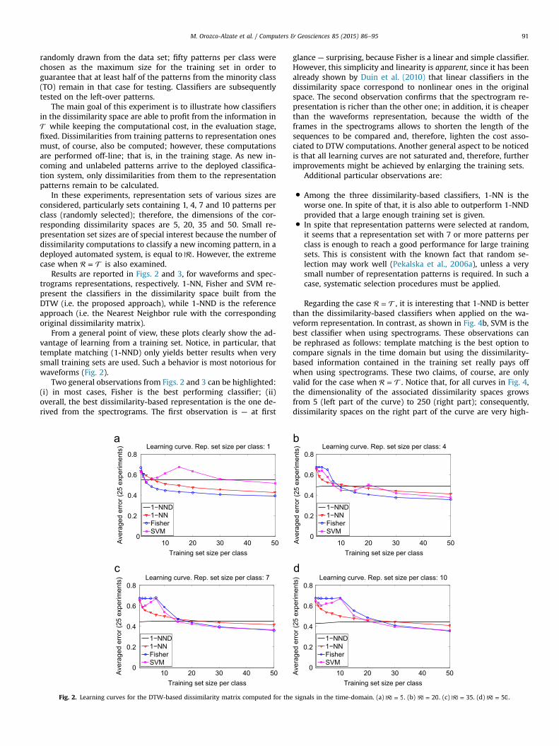
randomly drawn from the data set; fifty patterns per class werechosen as the maximum size for the training set in order toguarantee that at least half of the patterns from the minority class(TO) remain in that case for testing. Classifiers are subsequentlytested on the left-over patterns.

The main goal of this experiment is to illustrate how classifiersin the dissimilarity space are able to profit from the information in

while keeping the computational cost, in the evaluation stage,fixed. Dissimilarities from training patterns to representation onesmust, of course, also be computed; however, these computationsare performed off-line; that is, in the training stage. As new in-coming and unlabeled patterns arrive to the deployed classifica-tion system, only dissimilarities from them to the representationpatterns remain to be calculated.

In these experiments, representation sets of various sizes areconsidered, particularly sets containing 1, 4, 7 and 10 patterns perclass (randomly selected); therefore, the dimensions of the cor-responding dissimilarity spaces are 5, 20, 35 and 50. Small re-presentation set sizes are of special interest because the number ofdissimilarity computations to classify a new incoming pattern, in adeployed automated system, is equal to | |. However, the extremecase when = is also examined.

Results are reported in Figs. 2 and 3, for waveforms and spec-trograms representations, respectively. 1-NN, Fisher and SVM re-present the classifiers in the dissimilarity space built from theDTW (i.e. the proposed approach), while 1-NND is the referenceapproach (i.e. the Nearest Neighbor rule with the correspondingoriginal dissimilarity matrix).

From a general point of view, these plots clearly show the ad-vantage of learning from a training set. Notice, in particular, thattemplate matching (1-NND) only yields better results when verysmall training sets are used. Such a behavior is most notorious forwaveforms (Fig. 2).

Two general observations from Figs. 2 and 3 can be highlighted:(i) in most cases, Fisher is the best performing classifier; (ii)overall, the best dissimilarity-based representation is the one de-rived from the spectrograms. The first observation is — at first

10 20 30 40 500

0.2

0.4

0.6

0.8

Training set size per class

Ave

rage

d er

ror (

25 e

xper

imen

ts) Learning curve. Rep. set size per class: 1

1−NND1−NNFisherSVM

10 20 30 40 500

0.2

0.4

0.6

0.8


Ave

rage

d er

ror (

25 e

xper

imen



Fig. 2. Learning curves for the DTW-based dissimilarity matrix computed for the

glance — surprising, because Fisher is a linear and simple classifier.However, this simplicity and linearity is apparent, since it has beenalready shown by Duin et al. (2010) that linear classifiers in thedissimilarity space correspond to nonlinear ones in the originalspace. The second observation confirms that the spectrogram re-presentation is richer than the other one; in addition, it is cheaperthan the waveforms representation, because the width of theframes in the spectrograms allows to shorten the length of thesequences to be compared and, therefore, lighten the cost asso-ciated to DTW computations. Another general aspect to be noticedis that all learning curves are not saturated and, therefore, furtherimprovements might be achieved by enlarging the training sets.

Additional particular observations are:

�

Ave

rage

d er

ror (

25 e

xper

imen

ts)

Ave

rage

d er

ror (

25 e

xper

imen

ts)

sig

Among the three dissimilarity-based classifiers, 1-NN is theworse one. In spite of that, it is also able to outperform 1-NNDprovided that a large enough training set is given.

�
In spite that representation patterns were selected at random,it seems that a representation set with 7 or more patterns perclass is enough to reach a good performance for large trainingsets. This is consistent with the known fact that random se-lection may work well (Pekalska et al., 2006a), unless a verysmall number of representation patterns is required. In such acase, systematic selection procedures must be applied.
Regarding the case = , it is interesting that 1-NND is betterthan the dissimilarity-based classifiers when applied on the wa-veform representation. In contrast, as shown in Fig. 4b, SVM is thebest classifier when using spectrograms. These observations canbe rephrased as follows: template matching is the best option tocompare signals in the time domain but using the dissimilarity-based information contained in the training set really pays offwhen using spectrograms. These two claims, of course, are onlyvalid for the case when = . Notice that, for all curves in Fig. 4,the dimensionality of the associated dissimilarity spaces growsfrom 5 (left part of the curve) to 250 (right part); consequently,dissimilarity spaces on the right part of the curve are very high-

10 20 30 40 500

0.2

0.4

0.6

0.8


Learning curve. Rep. set size per class: 4


10 20 30 40 500

0.2

0.4

0.6

0.8


Learning curve. Rep. set size per class: 10


nals in the time-domain. (a) 5| | = . (b) 20| | = . (c) 35| | = . (d) 50| | = .

10 20 30 40 500

0.1

0.2

0.3

0.4

0.5

0.6


Ave

rage

d er

ror (

25 e

xper

imen



10 20 30 40 500

0.1

0.2

0.3

0.4

0.5

0.6


Ave

rage

d er

ror (

25 e

xper

imen



10 20 30 40 500

0.1

0.2

0.3

0.4

0.5

0.6


Ave

rage

d er

ror (

25 e

xper

imen



10 20 30 40 500

0.1

0.2

0.3

0.4

0.5

0.6


Ave

rage

d er

ror (

25 e

xper

imen



Fig. 3. Learning curves for the DTW-based dissimilarity matrix computed for the signal spectrograms (time/frequency-domain). (a) 5| | = . (b) 20| | = . (c) 35| | = . (d)50| | = .


dimensional and demand, to a deployed system, as many dissim-ilarity computations as dimensions.

4.3. Experiment 2

As explained in the previous sections, dissimilarity re-presentations based on a large training set can be computationallydemanding (Duin and Pekalska, 2012). Therefore, it is important toprune the representation set to a size significantly smaller thanthat of the training set. This second experiment consists in ex-amining curves for growing representation sets drawn from thetraining set that, in turn, corresponds to half of the data set; inother words, 50% of the data is used for training and the remaining50% for testing. Two systematic selection procedures — (i) forwardselection using the leave-one-out (LOO) 1-NN error as criterionand (ii) k-centres— as well as random selection are used; details oftheir implementations are not given here but can be found inPekalska et al. (2006a). Experiments, in this case, were repeatedmore times (50) in order to better capture the average behaviorwhen two random procedures are involved: partition into train-ing-test sets and the random selection itself. Results are displayed

10 20 30 40 500

0.2

0.4

0.6

0.8


Ave

rage

d er

ror (

25 e

xper

imen

ts) Learning curve. Rep. set = Train. set


Fig. 4. Learning curves for = . (a

in Fig. 5, for both the waveform and the spectrogramrepresentations.

The first evident observation is that dissimilarity-based classi-fiers are much better than template matching when using randomselection and k-centres; see Fig. 5a and b and Fig. 5e and f, re-spectively. Forward selection finds good representation sets for 1-NND that are difficult to be enhanced by providing the additionalinformation contained in the training sets; in fact, the only case —

for forward selection — in which a dissimilarity-based classifier isslightly better than 1-NND is the one in Fig. 5d. This confirms that1-NND is highly dependent on a carefully selected set of proto-types while classifiers in the dissimilarity space are not.

In spite of the superiority of forward selection, one must alsoconsider that its computational cost is larger due to its supervisedselection criterion: the minimization of the LOO 1-NN classifica-tion error. The other two procedures, in contrast, are unsupervisedbut still carried out in a class-wise way. The cheapest option is, ofcourse, random selection since just implies the generation of arandom permutation of indexes. Notice also that curves in Fig. 5turn flat after having included a certain number of prototypes in ;so, the computational demands associated to large representation

10 20 30 40 500

0.1

0.2

0.3

0.4

0.5

0.6


Ave

rage

d er

ror (

25 e

xper

imen

ts) Learning curve. Rep. set = Train. set


) Waveforms. (b) Spectrograms.

10 20 30 40 500

0.1

0.2

0.3

0.4

0.5

0.6

Representation set size

Ave

rage

d er

ror (

50 e

xper

imen

ts) Random selection

1−NND1−NNFisher

10 20 30 40 500

0.1

0.2

0.3

0.4

0.5

0.6


Ave

rage

d er

ror (

50 e

xper

imen

ts) Random selection

1−NND1−NNFisher

10 20 30 40 500

0.1

0.2

0.3

0.4

0.5


Ave

rage

d er

ror (

50 e

xper

imen

ts) Forward (LOO NN) selection

1−NND1−NNFisher

10 20 30 40 500

0.1

0.2

0.3

0.4


Ave

rage

d er

ror (

50 e

xper

imen

ts) Forward (LOO NN) selection

1−NND1−NNFisher

10 20 30 40 500

0.1

0.2

0.3

0.4

0.5


Ave

rage

d er

ror (

50 e

xper

imen

ts) Selection by k−centres

1−NND1−NNFisher

10 20 30 40 500

0.1

0.2

0.3

0.4

0.5

0.6


Ave

rage

d er

ror (

50 e

xper

imen

ts) Selection by k−centres

1−NND1−NNFisher

Fig. 5. Curves for growing representation set sizes. The entire training set, corresponding to half of the data set, is used for training the classifiers. (a) Random selection:waveforms. (b) Random selection: spectrograms. (c) Forward selection: waveforms. (d) Forward selection: spectrograms. (e) Selection by k-centres: waveforms. (f) Selectionby k-centres: spectrograms.

10 20 30 40 500

0.1

0.2

0.3

0.4

0.5

0.6


Ave

rage

d er

ror (

25 e

xper

imen

ts) Learning curve. Combined sets


10 20 30 40 500

0.1

0.2

0.3

0.4

0.5

0.6


Ave

rage

d er

ror (

25 e

xper

imen

ts) Learning curve. Combined sets


Fig. 6. Learning curves for the combined dissimilarity matrices. (a) Average combination of “waveformsþspectrograms” dissimilarities and (b) ”waveformsþspectro-gramsþspectra” dissimilarities.


set sizes are not compensated by a significant increase in classi-fication performance.

4.4. Experiment 3

This experiment is aimed at showing the effect on the

classification accuracies of the combination of different dissim-ilarity matrices, see Fig. 6. In particular, we considered the twodissimilarity matrices derived from the two representations (wa-veforms and spectrograms). Furthermore, we also considered an-other dissimilarity matrix, employing Euclidean distances betweenone-dimensional spectra, computed as described above. In both

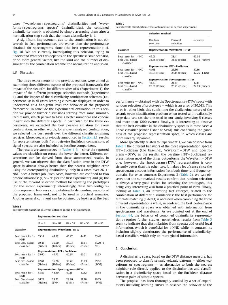
Table 2Best (lowest) classification errors obtained in the second experiment.

Selection method

Randomselection

Forwardselection

k-centres

Classifier Representation: WaveformþDTW

Best result for 1-NND 45.08 28.41 40.64Best Diss.-based

classifier33.46 (Fisher) 31.89 (Fisher) 32.98 (Fisher)

Representation: FFTþEuclideanBest result for 1-NND 41.63 26.36 57.36Best Diss.-based

classifier30.94 (Fisher) 28.14 (Fisher) 32.26 (1-NN)

Representation: SpectrogramsþDTWBest result for 1-NND 43.43 21.89 42.11Best Diss.-based

classifier20.01 (Fisher) 20.41 (Fisher) 24.63 (Fisher)


cases (“waveformsþspectrograms” dissimilarities and “wave-formsþspectrogramsþspectra” dissimilarities), the combineddissimilarity matrix is obtained by simply averaging them after anormalization step such that the mean dissimilarity is 1.

A significant improvement due to the combination is not ob-served; in fact, performances are worse than the performanceobtained for spectrograms alone (the best representation); cf.Fig. 3d. We are currently investigating this behavior, trying tounderstand whether this depends on the specific seismic scenario,or on more general factors, like the kind and the number of dis-similarities, the combination scheme, the normalization and so on.

4.5. Discussion

The three experiments in the previous sections were aimed atexamining three different aspects of the proposed framework: theimpact of the size of for different sizes of (Experiment 1), theimpact of the different prototype selection methods (Experiment2), and the impact of the dissimilarity combination schemes (Ex-periment 3): in all cases, learning curves are displayed, in order tounderstand at a fine-grain level the behavior of the proposedframework. To conclude the experimental evaluation, in this sec-tion we provide further discussions starting from some summar-ized results, which permit to have a better numerical and conciseinsight into the different aspects. In particular, for the three ex-periments, we extracted the best possible situation for everyconfiguration: in other words, for a given analyzed configuration,we selected the best result over the different classifiers/trainingset sizes. Moreover, as previously announced in Section 3.1, resultsfor representations built from pairwise Euclidean comparisons ofsignal spectra are also included as baseline comparisons.

The results are summarized in Tables 1–3 — since the reportedvalues are classification errors, the lower the better. Different ob-servations can be derived from these summarized results. Ingeneral, we can observe that the classification error in the DTWspace is almost always better than the nearest neighbor errorusing the corresponding dissimilarity: only in 4 cases over 26, 1-NND does a better job. Such cases, however, are confined to twoprecise situations: (i) = (for the first experiment), and (ii) theuse of the forward selection method for selecting the prototypes(for the second experiment): interestingly, these two configura-tions represent two very computationally demanding versions ofthe proposed framework, not to be used in practical scenarios.Another general comment can be obtained by looking at the best

Table 1Best (lowest) classification errors obtained in the first experiment.

Representation set sizes

5| | = 20| | = 35| | = 50| | = | | = | |

Classifier Representation: WaveformþDTW

Best result for 1-NND

55.18 48.92 45.27 44.11 35.43

Best Diss.-basedclassifier

39.48(Fisher)

36.00(Fisher)

35.93(Fisher)

35.61(Fisher)

41.20 (1-NN)

Representation: FFTþEuclideanBest result for 1-

NND55.60 46.73 40.88 40.51 31.33


42.61(Fisher)

36.26(Fisher)

33.72(Fisher)

33.09(Fisher)

29.58(SVM)

Representation: SpectrogramsþDTWBest result for 1-

NND53.87 44.50 40.11 37.52 28.53


36.22(Fisher)

23.71(SVM)

22.96(SVM)

21.70(Fisher)

29.13(SVM)

performance — obtained with the SpectrogramsþDTW space withrandom selection of prototypes — which is an error of 20.01%. Thiserror is rather high, this confirming the challenging nature of theseismic event classification problem when tested with realisticallylarge data sets (as the one used in our study, involving 5 classesand more than 1200 events). Finally, it is interesting to observethat the best classifier in the dissimilarity space is in most cases alinear classifier (either Fisher or SVM), this confirming the good-ness of the proposed representation space, in which classes aremore linearly separable.

More specifically related to Experiment 1, we can observe fromTable 1 the different behaviors of the three representation spaces:FFTþEuclidean (the baseline), WaveformþDTW and Spectro-gramsþDTW; in the results, the baseline (FFTþEuclidean) re-presentation most of the times outperforms the WaveformþDTWone; however, the SpectrogramþDTW representation is con-sistently better than the other two. It makes a lot of sense since thespectrogram encodes information from both time- and frequency-domain. For what concerns Experiment 2 (Table 2), we can ob-serve that the summarized results confirm that random selectionis always a very good choice for selecting the prototypes, thisbeing very interesting also from a practical point of view. Finally,looking at Table 3, an interesting fact emerges, related to thecombination of different dissimilarities: the best performance fortemplate matching (1-NND) is obtained when combining the threedifferent representations while, in contrast, the best performancein the dissimilarity space was obtained with information fromspectrograms and waveforms. As we pointed out at the end ofSection 4.4, the behavior of combined dissimilarity representa-tions requires further studies; nonetheless, results from Table 3seem to indicate that dissimilarities from spectra add useful localinformation, which is beneficial for 1-NND while, in contrast, itsinclusion slightly deteriorates the performance of dissimilarity-based classifiers which rely on more global information.

5. Conclusion

A dissimilarity space, based on the DTW distance measure, hasbeen proposed to classify seismic volcanic patterns — either wa-veforms or spectrograms — as alternative to both the nearestneighbor rule directly applied to the dissimilarities and classifi-cation in a dissimilarity space based on the Euclidean distancebetween pairs of seismic spectra.

The proposal has been thoroughly studied by a set of experi-ments including learning curves to observe the behavior of the

Table 3Best (lowest) classification errors obtained in the third experiment.

Combined dissimilarity-based representations

Classifier “Waveformsþspectrograms” “Waveformsþspectrogramsþspectra”

Best result for 1-NND 41.17 37.24Best Diss.-based classifier 24.53 (Fisher) 25.27 (Fisher)


classification system over different training set sizes, curves tostudy the behavior for different dimensionalities of the DTW-based dissimilarity space and analyses on the possibilities of en-hancing the classification performance by combining dissimilarityrepresentations computed for different modalities of the seismicdata (waveforms, spectra, spectrograms) or dissimilarity measures(DTW, Euclidean).

Results clearly showed the advantage of learning from atraining set by building the DTW-based representation space,particularly when starting its construction from spectrograms.Low-dimensional versions of the proposed representation spaceallow to reduce the computational demands of a deployed systemwhile preserving good enough classification performances;moreover, linear classifiers in the DTW-based dissimilarity spaceyield satisfactory classification accuracies as expected. Eventhough attempts to profit from the averaged combination of dif-ferent dissimilarity representations were made, enhancements inthe performances by applying this strategy were not observed.Further studies on this topic may be worthwhile.

Acknowledgements

Support from Dirección de Investigación - Sede Manizales(DIMA), Universidad Nacional de Colombia, is acknowledged aswell as the Cooperint program from University of Verona. In ad-dition, the authors would like to thank Programa de FormaciónDoctoral en Colombia - Becas COLCIENCIAS (Convocatoria 617 de2013 - Convenio Especial No. 0656-2013, entre COLCIENCIAS y laUniversidad Nacional de Colombia) for supporting the secondauthor, and also the staff members from OVSM for providing thedata set.

References

Castro-Cabrera, P.A., Orozco-Alzate, M., Adami, A., Bicego, M., Londoño-Bonilla, J.M.,Castellanos-Domínguez, C.G., November 2014. A comparison between time–frequency and cepstral feature representations for seismic-volcanic patternclassification. In: Bayro-Corrochano, E., Hancock, E. (Eds.), Progress in PatternRecognition, Image Analysis, Computer Vision, and Applications. Proceedings ofthe 19th Iberoamerican Congress on Pattern Recognition CIARP 2014, LectureNotes in Computer Science, IAPR, vol. 8827. Springer, Heidelberg, pp. 440–447.

Duin, R.P.W., Loog, M., Pekalska, E., Tax, D.M.J., 2010. Feature-based dissimilarityspace classification. In: Ünay, D., Çataltepe, Z., Aksoy, S. (Eds.), RecognizingPatterns in Signals, Speech, Images and Videos: ICPR 2010 Contests, LectureNotes in Computer Science, vol. 6388. Springer, Berlin, Heidelberg, pp. 46–55.

Duin, R.P.W., Pekalska, E., 2007. The science of pattern recognition, achievementsand perspectives. In: Duch, W., Mańdziuk, J. (Eds.), Challenges for Computa-tional Intelligence. Studies in Computational Intelligence, vol. 63. Springer,Berlin, pp. 221–259.

Duin, R.P.W., Pekalska, E., 2012. The dissimilarity space: bridging structural andstatistical pattern recognition. Pattern Recognit. Lett. 33 (7), 826–832.

Duin, R.P.W., Pekalska, E., Loog, M., 2013. Non-Euclidean dissimilarities: causes,embedding and informativeness. In: Pelillo, M. (Ed.), Similarity-Based PatternAnalysis and Recognition. Advances in Computer Vision and Pattern Recogni-tion. Springer, London, pp. 13–44.

Ibba, A., Duin, R.P.W., Lee, W.-J., 2010. A study on combining sets of differentlymeasured dissimilarities. In: 20th International Conference on Pattern Re-cognition (ICPR 2010), pp. 3360–3363.

Lemire, D., 2009. Faster retrieval with a two-pass dynamic-time-warping lowerbound. Pattern Recognit. 42 (9), 2169–2180.

Lin, J., Williamson, S., Borne, K.D., DeBarr, D., 2012. Pattern recognition in timeseries. In: Way, M.J., Scargle, J.D., Ali, K.M., Srivastava, A.N. (Eds.), Advances inMachine Learning and Data Mining for Astronomy. Data Mining and KnowledgeDiscovery Series. CRC Press, Boca Raton, FL, pp. 617–646 (Chapter 28).

Orozco-Alzate, M., García-Ocampo, M.E., Duin, R.P.W., Castellanos-Domínguez, C.G.,2006. Dissimilarity-based classification of seismic volcanic signals at Nevadodel Ruiz volcano. Earth Sci. Res. J. 10 (December (2)), 57–65.

Pekalska, E., Duin, R.P.W., 2005. The dissimilarity representation for pattern re-cognition: foundations and applications. In: Machine Perception and ArtificialIntelligence, vol. 64, World Scientific, Singapore.

Pekalska, E., Duin, R.P.W., Paclík, P., 2006a. Prototype selection for dissimilarity-based classifiers. Pattern Recognit. 39 (2), 189–208 (Special issue: ComplexityReduction).

Pekalska, E., Harol, A., Duin, R.P.W., Spillmann, B., Bunke, H., 2006b. Non-Euclideanor non-metric measures can be informative. In: Yeung, D.-Y., Kwok, J., Fred, A.,Roli, F., de Ridder, D. (Eds.), Structural, Syntactic, and Statistical Pattern Re-cognition Joint IAPR International Workshops, SSPR 2006 and SPR 2006, Lec-ture Notes in Computer Science, vol. 4109. Springer, Berlin, Heidelberg,pp. 871–880.

Pelillo, M. (Ed.), 2013. Similarity-Based Pattern Analysis and Recognition. Advancesin Computer Vision and Pattern Recognition. Springer, London, UK.

Plasencia-Calaña, Y., Cheplygina, V., Duin, R.P.W., García-Reyes, E.B., Orozco-Alzate,M., Tax, D.M.J., Loog, M., July 2013. On the informativeness of asymmetricdissimilarities. In: Hancock, E.R., Pelillo, M. (Eds.), Similarity-Based Pattern andRecognition: Proceedings of the Second International Workshop, SIMBAD 2013,Lecture Notes in Computer Science, vol. 7953. Springer, Berlin, Germany,pp. 75–89.

Porro-Muñoz, D., Talavera, I., Duin, R.P.W., Orozco-Alzate, M., 2011. Combiningdissimilarities for three-way data classification. Comput. Sist. 15 (1), 117–127.

Schilling, R.J., Harris, S.L., 2012. Fundamentals of Digital Signal Processing usingMATLAB, 2nd edition. Cengage Learning, Stamford, CT.

Telesca, L., Lovallo, M., Chamoli, A., Dimri, V., Srivastava, K., 2013. Fisher–Shannonanalysis of seismograms of tsunamigenic and non-tsunamigenic earthquakes.Physica A: Stat. Mech. Appl. 392 (16), 3424–3429.

Telesca, L., Lovallo, M., Kiszely, M.M., Toth, L., 2011. Discriminating quarry blastsfrom earthquakes in Vértes Hills (Hungary) by using the Fisher–Shannonmethod. Acta Geophys. 59 (5), 858–871.

Theodoridis, S., Koutroumbas, K., 2009. Pattern Recognition, 4th edition. AcademicPress, Burlington, MA.

Wang, Q., August 2013. Dynamic TimeWarping (DTW) Package. Available at ⟨http://www.mathworks.com/matlabcentral/fileexchange/⟩.

http://refhub.elsevier.com/S0098-3004(15)00138-7/sbref1









































































http://www.mathworks.com/matlabcentral/fileexchange/

http://www.mathworks.com/matlabcentral/fileexchange/

The DTW-based representation space for seismic pattern...

Documents

Transcript of The DTW-based representation space for seismic pattern...