
The dissertation of Poe Xing is approved: Date University ...epxing/papers/thesis.pdf · M.S....
260
Probabilistic graphical models and algorithms for genomic analysis by Poe Xing B.S. (Tsinghua University) 1993 M.S. (Rutgers University) 1998 Ph.D. (Rutgers University) 1999 A dissertation submitted in partial satisfaction of the requirements for the degree of Doctor of Philosophy in Computer Science in the GRADUATE DIVISION of the UNIVERSITY OF CALIFORNIA, BERKELEY Committee in charge: Professor Richard Karp, co-Chair Professor Michael Jordan, co-Chair Professor Stuart Russell, co-Chair Professor Gene Myers Professor Terry Speed Fall 2004
Transcript of The dissertation of Poe Xing is approved: Date University ...epxing/papers/thesis.pdf · M.S....

Probabilistic graphical models and algorithms for genomic analysis
by
Poe Xing
B.S. (Tsinghua University) 1993M.S. (Rutgers University) 1998
Ph.D. (Rutgers University) 1999
A dissertation submitted in partial satisfactionof the requirements for the degree of
Doctor of Philosophy
in
Computer Science
in the
GRADUATE DIVISION
of the
UNIVERSITY OF CALIFORNIA, BERKELEY
Committee in charge:
Professor Richard Karp, co-ChairProfessor Michael Jordan, co-ChairProfessor Stuart Russell, co-Chair
Professor Gene MyersProfessor Terry Speed
Fall 2004

The dissertation of Poe Xing is approved:
co-Chair Date
co-Chair Date
co-Chair Date
Date
Date
University of California, Berkeley
Fall 2004

Probabilistic graphical models and algorithms for genomic analysis
Copyright c© 2004
by
Poe Xing

Abstract
Probabilistic graphical models and algorithms for genomic analysis
by
Poe Xing
Doctor of Philosophy in Computer Science
University of California, Berkeley
Professor Richard Karp, co-Chair
Professor Michael Jordan, co-Chair
Professor Stuart Russell, co-Chair
In this thesis, I discuss two probabilistic modeling problems arising in metazoan genomic anal-
ysis: identifying motifs andcis-regulatory modules (CRMs) from transcriptional regulatory se-
quences, and inferring haplotypes from genotypes of single nucleotide polymorphisms. Motif and
CRM identification is important for understanding the gene regulatory network underlying meta-
zoan development and functioning. I discuss a modular Bayesian model that captures rich structural
characteristics of the transcriptional regulatory sequences and supports a variety of motif detection
tasks. Haplotype inference is essential for the understanding of genetic variation within and among
populations, with important applications to the genetic analysis of disease propensities. I discuss a
Bayesian model based on a prior distribution constructed from a Dirichlet process – a nonparamet-
ric prior which provides control over the size of the unknown pool of population haplotypes, and
on a likelihood function that allows statistical errors in the haplotype/genotype relationship. Our
models use the “probabilistic graphical model” formalism, a formalism that exploits the conjoined
capabilities of graph theory and probability theory to build complex models out of simpler pieces.
I discuss the mathematical underpinnings for the models, how they formally incorporate biolog-
ical prior knowledge about the data, and I present a generalized mean field theory and a generic
algorithm for approximate inference on such models.
1

co-ChairDate
co-ChairDate
co-ChairDate
2

Dedicate to my wife — Wei
and
to my parents
for encouraging me
to pursue my dream
and
for sharing my joy and frustration
in this endeavor
i

Acknowledgements
I wish to thank my advisers at Berkeley, Richard Karp, Michael Jordan and Stuart Russell, for
their kindness, patience, and cooperativeness in working as a “dream team” along with me to make
possible a smooth transformation for me from a novice to a professional in computer science during
the past five years, and for giving me so much freedom to discover and explore new subjects in ma-
chine learning, statistics and computational biology. I thank Richard Karp for his generous support,
invaluable trust, inspiring discussions and insightful suggestions on my research in computational
biology, and for being a great friend and a source of encouragement and understanding. I thank
Michael Jordan for his great patience and unparalleled technical guidance early in my development,
and his inspiration, enthusiasm and encouragement on my research in machine learning. I am also
greatly indebted to Stuart Russell, for sharing with me his wisdom and humor, his insightful cri-
tiques and stimulating ideas, and for his extensive technical and moral support on my research and
career development. A Ph.D. under their mentorship is the experience of a lifetime.
My other committee members have also been very supportive. Gene Myers has been a warm
supporter on my endeavor in computational biology, and a source of new problems, new ideas and
objective opinions from the non-machine-learning community. Terry Speed inspired my interest
in statistical genetics, and has also brought lots of useful outsider’s perspective to the thesis. In
particular, it was in writing a term paper for one of his classes that I worked out the first piece of
this dissertation — the new motif detection model.
I would like to thank my many friends and colleagues at Berkeley with whom I have had
the pleasure of working over the years. These include Eyal Amir, David Blei, Nando de Freitas,
Bhaskara Marthi, Brian Milch, Erik Miller, Kevin Murphy, Andrew Ng, Xuanlong Nguyen, Mark
Paskin, Matthias Seeger, Yee-Whye Teh, Martin Wainwright, Yair Weiss, Andy Zimdars, Alice
Zheng, and all the members of the SAIL and RUGS groups. Their encouragement and friendship
and their help have brought me incredible joy during my Berkeley days. I particularly want to thank
Brian Milch for his critical reading of this thesis, which greatly improved its clarity and readability
ii

(although any remaining errors in the thesis are of course my fault).
I would also like to thank Eric Horvitz, Tanveer Syeda-Mahmood and Jeonghee Yi for hiring
me as an intern at Microsoft Research in 2001, as a consultant at IBM Research in 2001, and
as an instructor at IBM Research during 2001-2002, respectively, during which I gained valuable
experience in industrial R&D and in advanced teaching.
I want to extent my gratitude to other friends in Soda hall, on campus, and beyond for friendship
and support. Finally, I wound like to thank my wife Wei for bearing with my countless weekend
and late night stays in the office, for listening to my wild ideas and endless details, and for her
encouragement on my work with love, patience and understanding.
iii
Contents
1 Introduction 1
1.1 Genomic Analysis and the Graphical Model Approach. . . . . . . . . . . . . . . 2
1.1.1 The Architecture and Function of the Genome. . . . . . . . . . . . . . . . 2
1.1.2 The Populational Diversity and Evolution of the Genome. . . . . . . . . . 4
1.1.3 Probabilistic Graphical Models and Genomic Analysis. . . . . . . . . . . 7
1.2 Thesis Overview . . . . . . . . . . . . . . . . . . . . . . . . . . . . . . . . . . . 10
1.2.1 The Problem. . . . . . . . . . . . . . . . . . . . . . . . . . . . . . . . . 10
1.2.2 Contributions of This Thesis. . . . . . . . . . . . . . . . . . . . . . . . . 12
1.2.3 Importance for Bioinformatics, Computer Science and Statistics. . . . . . 14
1.3 Technical Results of This Thesis. . . . . . . . . . . . . . . . . . . . . . . . . . . 17
1.3.1 A Modular Parametric Bayesian Model for Transcriptional Regulatory Se-
quences. . . . . . . . . . . . . . . . . . . . . . . . . . . . . . . . . . . . 17
1.3.1.1 Profile Bayesian models for motif sequence pattern. . . . . . . 18
1.3.1.2 Bayesian HMM for motif organization. . . . . . . . . . . . . . 20
1.3.1.3 The LOGOS model. . . . . . . . . . . . . . . . . . . . . . . . 21
1.3.2 A Non-Parametric Bayesian Model for Single Nucleotide Polymorphisms. 22
1.3.3 The Generalized Mean Field Algorithms for Variational Inference. . . . . 24
1.4 Thesis Organization. . . . . . . . . . . . . . . . . . . . . . . . . . . . . . . . . . 26
2 Modeling Transcriptional Regulatory Sequences for Motif Detection
iv

28
2.1 Biological Foundations and Motivations. . . . . . . . . . . . . . . . . . . . . . . 29
2.2 Problem Formulation. . . . . . . . . . . . . . . . . . . . . . . . . . . . . . . . . 33
2.2.1 Motif Representation. . . . . . . . . . . . . . . . . . . . . . . . . . . . . 33
2.2.2 Computational Tasks forIn SilicoMotif Detection . . . . . . . . . . . . . 35
2.2.3 General Setting and Notation. . . . . . . . . . . . . . . . . . . . . . . . . 37
2.2.4 TheLOGOS Framework: a Modular Formulation. . . . . . . . . . . . . 38
2.3 An Overview of Related Work. . . . . . . . . . . . . . . . . . . . . . . . . . . . 40
2.3.1 Background Models. . . . . . . . . . . . . . . . . . . . . . . . . . . . . 40
2.3.1.1 The models . . . . . . . . . . . . . . . . . . . . . . . . . . . . 40
2.3.1.2 The use of background models. . . . . . . . . . . . . . . . . . 41
2.3.2 Local Models — for the Consensus and Stochasticity of Motif Sites. . . . 43
2.3.2.1 Product multinomial model. . . . . . . . . . . . . . . . . . . . 43
2.3.2.2 Constrained PM models. . . . . . . . . . . . . . . . . . . . . . 44
2.3.2.3 Motif Bayesian networks. . . . . . . . . . . . . . . . . . . . . 46
2.3.3 Global Models — for the Genomic Distributions of Motif Sites. . . . . . 47
2.3.3.1 Theoopsandzoopsmodel . . . . . . . . . . . . . . . . . . . . 47
2.3.3.2 General uniform and independent models. . . . . . . . . . . . . 49
2.3.3.3 The dictionary model. . . . . . . . . . . . . . . . . . . . . . . 51
2.3.3.4 The sliding-window approaches. . . . . . . . . . . . . . . . . . 53
2.3.3.5 The hidden Markov model. . . . . . . . . . . . . . . . . . . . 54
2.3.4 Other Models. . . . . . . . . . . . . . . . . . . . . . . . . . . . . . . . . 55
2.3.4.1 Comparative genomic approach. . . . . . . . . . . . . . . . . . 56
2.3.4.2 Joint models for motifs and expression profiles. . . . . . . . . . 58
2.3.5 Summary: Understanding Motif Detection Algorithms. . . . . . . . . . . 59
2.4 MotifPrototyper: Modeling Canonical Meta-Sequence Features Shared in a Motif
Family . . . . . . . . . . . . . . . . . . . . . . . . . . . . . . . . . . . . . . . . . 61
v

2.4.1 Categorization of Motifs Based on Biological Classification of DNA Bind-
ing Proteins. . . . . . . . . . . . . . . . . . . . . . . . . . . . . . . . . . 63
2.4.2 HMDM: a Bayesian Profile Model for Motif Families. . . . . . . . . . . 67
2.4.2.1 Training a MotifPrototyper. . . . . . . . . . . . . . . . . . . . 70
2.4.3 Mixture of MotifPrototypers. . . . . . . . . . . . . . . . . . . . . . . . . 71
2.4.3.1 Classifying motifs. . . . . . . . . . . . . . . . . . . . . . . . . 71
2.4.3.2 Bayesian estimation of PWMs. . . . . . . . . . . . . . . . . . 72
2.4.3.3 Semi-unsupervisedde novomotif detection. . . . . . . . . . . . 73
2.4.4 Experiments . . . . . . . . . . . . . . . . . . . . . . . . . . . . . . . . . 73
2.4.4.1 Parameter estimation. . . . . . . . . . . . . . . . . . . . . . . 74
2.4.4.2 Motif classification . . . . . . . . . . . . . . . . . . . . . . . . 76
2.4.4.3 PWM estimation and motif scoring. . . . . . . . . . . . . . . . 77
2.4.4.4 De novomotif discovery. . . . . . . . . . . . . . . . . . . . . . 79
2.4.5 Summary and Discussion. . . . . . . . . . . . . . . . . . . . . . . . . . . 84
2.5 CisModuler: Modeling the Syntactic Rules of Motif Organization. . . . . . . . . 85
2.5.1 TheCisModulerHidden Markov Model. . . . . . . . . . . . . . . . . . . 86
2.5.2 Bayesian HMM. . . . . . . . . . . . . . . . . . . . . . . . . . . . . . . . 89
2.5.3 Markov Background Models. . . . . . . . . . . . . . . . . . . . . . . . . 91
2.5.4 Posterior Decoding Algorithms for Motif Scan. . . . . . . . . . . . . . . 91
2.5.4.1 The baseline algorithm. . . . . . . . . . . . . . . . . . . . . . 91
2.5.4.2 Bayesian inference and learning. . . . . . . . . . . . . . . . . . 92
2.5.5 Experiments . . . . . . . . . . . . . . . . . . . . . . . . . . . . . . . . . 93
2.5.5.1 MAP prediction of motifs/CRMs. . . . . . . . . . . . . . . . . 95
2.5.5.2 Motif/CRM prediction via thresholding posterior probability profile96
2.5.6 Summary and Discussion. . . . . . . . . . . . . . . . . . . . . . . . . . . 99
2.6 LOGOS: for Semi-unsupervisedde novoMotif Detection . . . . . . . . . . . . . 100
2.6.1 Experiments . . . . . . . . . . . . . . . . . . . . . . . . . . . . . . . . .102
vi

2.6.1.1 Performance on semi-realistic sequence data. . . . . . . . . . . 102
2.6.1.2 Motif detection in yeast promoter regions. . . . . . . . . . . . . 105
2.6.1.3 Motif detection inDrosophilaregulatory DNAs . . . . . . . . . 106
2.7 Conclusions. . . . . . . . . . . . . . . . . . . . . . . . . . . . . . . . . . . . . .109
3 Modeling Single Nucleotide Polymorphisms for Haplotype Inference
111
3.1 Biological Foundations and Motivation. . . . . . . . . . . . . . . . . . . . . . . . 112
3.2 Problem Formulation and Overview of Related Work. . . . . . . . . . . . . . . . 114
3.2.1 Baseline Finite Mixture Model and the EM Approach. . . . . . . . . . . . 116
3.2.2 Bayesian Methods via MCMC. . . . . . . . . . . . . . . . . . . . . . . . 117
3.2.2.1 Simple Dirichlet priors . . . . . . . . . . . . . . . . . . . . . . 117
3.2.2.2 The coalescent prior. . . . . . . . . . . . . . . . . . . . . . . . 118
3.2.3 Bayesian Network Prior. . . . . . . . . . . . . . . . . . . . . . . . . . .118
3.2.4 Summary and Prelude to Our Approach. . . . . . . . . . . . . . . . . . . 120
3.3 Haplotype Inference via the Dirichlet Process. . . . . . . . . . . . . . . . . . . . 121
3.3.1 Dirichlet Process Mixture. . . . . . . . . . . . . . . . . . . . . . . . . . 122
3.3.2 DP-Haplotyper: a Dirichlet Process Mixture Model for Haplotypes. . . . 123
3.3.3 Haplotype Modeling Given Partial Pedigree. . . . . . . . . . . . . . . . . 126
3.4 Experimental Results. . . . . . . . . . . . . . . . . . . . . . . . . . . . . . . . .130
3.4.1 Simulated Data. . . . . . . . . . . . . . . . . . . . . . . . . . . . . . . .130
3.4.2 Real Data. . . . . . . . . . . . . . . . . . . . . . . . . . . . . . . . . . .131
3.5 Conclusions and Discussions. . . . . . . . . . . . . . . . . . . . . . . . . . . . .133
4 Probabilistic Inference I: Deterministic Algorithms 136
4.1 Background. . . . . . . . . . . . . . . . . . . . . . . . . . . . . . . . . . . . . .137
4.1.1 Notation . . . . . . . . . . . . . . . . . . . . . . . . . . . . . . . . . . .140
vii
4.2 Exact Inference Algorithms. . . . . . . . . . . . . . . . . . . . . . . . . . . . . .141
4.2.1 The Junction Tree Algorithm. . . . . . . . . . . . . . . . . . . . . . . . . 141
4.3 Approximate Inference Algorithms. . . . . . . . . . . . . . . . . . . . . . . . . . 145
4.3.1 Cluster-factorizable Potentials. . . . . . . . . . . . . . . . . . . . . . . . 145
4.3.2 Exponential Representations. . . . . . . . . . . . . . . . . . . . . . . . . 146
4.3.3 Lower Bounds of General Exponential Functions. . . . . . . . . . . . . . 147
4.3.3.1 Lower bounding probabilistic invariants. . . . . . . . . . . . . 149
4.3.4 A General Variational Principle for Probabilistic Inference. . . . . . . . . 150
4.3.4.1 Variational representation. . . . . . . . . . . . . . . . . . . . . 151
4.3.4.2 Mean field methods. . . . . . . . . . . . . . . . . . . . . . . . 152
4.3.4.3 Belief propagation. . . . . . . . . . . . . . . . . . . . . . . . . 154
4.4 Generalized Mean Field Inference. . . . . . . . . . . . . . . . . . . . . . . . . . 155
4.4.1 GMF Theory and Algorithm. . . . . . . . . . . . . . . . . . . . . . . . . 156
4.4.1.1 Naive mean field approximation. . . . . . . . . . . . . . . . . . 156
4.4.1.2 Generalized mean field theory. . . . . . . . . . . . . . . . . . . 158
4.4.2 A more general version of GMF theory. . . . . . . . . . . . . . . . . . . 163
4.4.3 A Generalized Mean Field Algorithm. . . . . . . . . . . . . . . . . . . . 164
4.4.4 Experimental Results. . . . . . . . . . . . . . . . . . . . . . . . . . . . .165
4.5 Graph Partition Strategies for GMF Inference. . . . . . . . . . . . . . . . . . . . 169
4.5.1 Bounds on GMF Approximation. . . . . . . . . . . . . . . . . . . . . . . 171
4.5.2 Variable Clustering via Graph Partitioning. . . . . . . . . . . . . . . . . . 172
4.5.2.1 Graph partitioning. . . . . . . . . . . . . . . . . . . . . . . . . 172
4.5.2.2 Semi-definite relaxation of GP. . . . . . . . . . . . . . . . . . 174
4.5.2.3 Finding a closest feasible solution. . . . . . . . . . . . . . . . . 176
4.5.3 Experimental Results. . . . . . . . . . . . . . . . . . . . . . . . . . . . .177
4.5.3.1 Partitioning random graphs. . . . . . . . . . . . . . . . . . . . 177
4.5.3.2 Single-node marginals. . . . . . . . . . . . . . . . . . . . . . . 178
viii

4.5.3.3 Bounds on the log partition function. . . . . . . . . . . . . . . 179
4.6 Extensions of GMF. . . . . . . . . . . . . . . . . . . . . . . . . . . . . . . . . .181
4.6.1 Higher Order Mean Field Approximation. . . . . . . . . . . . . . . . . . 181
4.6.2 Alternative Tractable Subgraphs. . . . . . . . . . . . . . . . . . . . . . . 182
4.6.3 Alternative Graph Partitioning Schemes. . . . . . . . . . . . . . . . . . . 182
4.7 Application to theLOGOS Model . . . . . . . . . . . . . . . . . . . . . . . . . . 183
4.7.1 A GMF Algorithm for Bayesian Inference inLOGOS . . . . . . . . . . . 184
4.7.2 Experimental Results. . . . . . . . . . . . . . . . . . . . . . . . . . . . .186
4.7.2.1 Convergence behavior of GMF. . . . . . . . . . . . . . . . . . 186
4.7.2.2 A comparison of GMF and the Gibbs sampler for motif inference187
4.8 Conclusions and Discussions. . . . . . . . . . . . . . . . . . . . . . . . . . . . .188
5 Probabilistic Inference II: Monte Carlo Algorithms 191
5.1 A Brief Overview of Monte Carlo Methods. . . . . . . . . . . . . . . . . . . . . 191
5.2 A Gibbs Sampling Algorithm forLOGOS . . . . . . . . . . . . . . . . . . . . . . 193
5.2.1 TheCollapsedGibbs Sampler. . . . . . . . . . . . . . . . . . . . . . . . 193
5.2.2 Convergence Diagnosis. . . . . . . . . . . . . . . . . . . . . . . . . . . .195
5.3 Markov Chain Monte Carlo for Haplotype Inference. . . . . . . . . . . . . . . . 196
5.3.1 A Gibbs Sampling Algorithm. . . . . . . . . . . . . . . . . . . . . . . . 197
5.3.2 A Metropolis-Hasting Sampling Algorithm. . . . . . . . . . . . . . . . . 201
5.3.3 A Sketch of MCMC Strategies for the Pedi-haplotyper model. . . . . . . 202
5.3.4 Summary. . . . . . . . . . . . . . . . . . . . . . . . . . . . . . . . . . .204
5.4 Conclusion . . . . . . . . . . . . . . . . . . . . . . . . . . . . . . . . . . . . . .205
6 Conclusions 207
6.1 Conclusions from This Work. . . . . . . . . . . . . . . . . . . . . . . . . . . . .207
6.2 Future Work. . . . . . . . . . . . . . . . . . . . . . . . . . . . . . . . . . . . . .208
ix

6.2.1 Modeling Gene Regulation Networks of Higher Eukaryotes in Light of Sys-
tems Biology and Comparative Genomics. . . . . . . . . . . . . . . . . . 208
6.2.2 Genetic Inference and Application Based on Polymorphic Markers. . . . . 211
6.2.3 Automated Inference in General Graphical Models. . . . . . . . . . . . . 213
A More details on inference and learning for motif models 215
A.1 Multinomial Distributions and Dirichlet Priors. . . . . . . . . . . . . . . . . . . . 215
A.2 Estimating Hyper-Parameters in the HMDM Model. . . . . . . . . . . . . . . . . 217
A.3 Computing the Expected Sufficient Statistics in the Global HMM. . . . . . . . . . 219
A.4 Bayesian Estimation of Multinomial Parameters in the HMDM Model. . . . . . . 220
B Proofs 222
B.1 Theorem2: GMF approximation. . . . . . . . . . . . . . . . . . . . . . . . . . .222
B.2 Theorem5: GMF bound on KL divergence. . . . . . . . . . . . . . . . . . . . . 224
x

Chapter 1
Introduction
Understanding the structure and functional organization of the genome is a fundamental problem
in biology. This thesis introduces new computational statistical approaches for analyzing two par-
ticular types of genomic data: gene regulatory sequences, and single nucleotide polymorphisms.
It presents the methodology of applying theprobabilistic graphical modelformalism to designing
novel parametric and non-parametric Bayesian models for genomic data, in accordance with bio-
logical prior knowledge or genetic hypotheses about the population of subjects under investigation.
In particular, it presents algorithms for the problems ofmotif detectionandhaplotype inference, and
develops the general theory and algorithms ofgeneralized mean field approximationfor variational
inferenceon large-scale, hybrid, multivariate probabilistic models.
Although the major goal of this thesis is to develop probabilistic models and computational
algorithms for deciphering biological data and exploring the mechanisms and evolution of biological
systems based on mathematical principles, most of the ideas and results reported here can also
serve as building blocks of generic intelligent systems for a wide range of applications that involve
predictive understanding and reasoning under uncertainty.
1
1.1 Genomic Analysis and the Graphical Model Approach
1.1 Genomic Analysis and the Graphical Model Approach
1.1.1 The Architecture and Function of the Genome
According to the central dogma, the genetic information that determines the functional and mor-
phological properties of the cells in a living organism is encoded in the DNA genome[Crick, 1970].
Biochemically, DNAs are double-stranded macromolecules representable as a pair of long comple-
mentary sequences of characters — A, T, G and C, denoting four kinds of basic elements, known as
nucleotides, that make up the DNA molecules. Residing in (and inherited via) the DNA molecules,
are a rich set of coding sequences referred to asgenes, which determine the structures and functions
of an essential set of biopolymer molecules, mostly proteins, but also including RNAs, which are
the main determinants of various cellular and physiological activities taking place in a living sys-
tem, such as biochemical catalysis, signal transduction, cellular defense, etc.[Lewin, 2003]. Also
abundant in the DNAs are a large number of so-called non-coding sequences, whose role was orig-
inally thought to be purely structural (e.g., serving as the physical scaffold of achromosome—
a long thread of DNA tightly packaged with the aid of several auxiliary proteins), but have been
recently discovered to play essential roles in the cellular implementation of thegene regulation
network[Davidson, 2001; Albertset al., 2002].
DNAs usually reside in the nucleus (or the nuclear region for prokaryotic organisms) of the
cell. Via a process calledtranscription(to be explained shortly), some genes in the DNA genome
are copied to molecules called messenger RNA (mRNA), which can travel out of the nucleus to
the protein synthesis apparatus, where proteins are assembled based on the coding information car-
ried by mRNA via a process calledtranslation [Alberts et al., 2002]. Although different cells of
an organism have the same DNA genome, it is well known that they have different protein com-
position and perform different functions[Davidson, 2001]. For example, red blood cells are rich
in hemoglobins that can carry oxygen, whereas muscle cells contain a large number of myosins
for muscular contraction. Even the same cell may bear different protein contents at different times
during its life span. This kind of diversity is a consequence of spatially and temporally regulated
2

1.1 Genomic Analysis and the Graphical Model Approach
expression of genes. It is believed that much of the information that determines when and in what
cellular environment a gene is expressed is encoded in certain genomic sequences, which possibly
account for a major portion of the total sequence of the genome, especially in the higher eukaryotes,
such as human[Davidson, 2001; Michelson, 2002].
Figure 1.1: The transcriptional regulatory machinery ( adapted from[Wasserman and Sandelin, 2004] ). TFBS: transcrip-tion factor binding site, CRM:cis-regulatory module; chromatin: a long, extended thread of DNA packed with histoneproteins.
The creation of diverse cell types from an invariant set of genes is governed by complex bio-
chemical processes that regulate gene activities. Transcription, the initial step of gene expression,
is central to the regulatory mechanisms. Transcription refers to the process of making a single-
stranded mRNA molecule using one of the DNA strands as template. The timing and volume of
transcription are controlled by complex transcription regulatory machinery made up of both protein
and DNA elements[Ptashne, 1988; Ptashne and Gann, 1997]. As shown in Fig.1.1, the signals that
activate or suppress the transcription of a gene are physically mediated by different types of gene
regulatory proteins calledtranscription factors(TFs). To bring these signals into effect on a target
3

1.1 Genomic Analysis and the Graphical Model Approach
gene at a specific time in a specific cell, certain TFs must recognize specific binding sites in the
vicinity of the target gene, so that they can jointly interact with the basal transcription apparatus,
made up of an RNA polymerase and some general TFs, to turn on or off transcription in the right
physiological/developmental context.
DNA motifsare the protein binding sites on DNA sequences that can be recognized by specific
TFs to integrate complex gene regulatory signals (hence they are also referred to as transcription
factor binding sites, or TFBS). These sites are usually located in the vicinity of the transcription
initiation sites of the genes under their regulation — an extended sequence region generally re-
ferred to as thetranscriptional regulatory region[Lewin, 2003]. Depending on which organism the
genomic sequences are from, the complexities of the transcriptional regulatory regions vary signifi-
cantly. Their lengths range from a few hundred base pairs (e.g, in simple bacteria such as E. coli) to
over several hundred thousand base pairs (e.g., in more complex insects such asDrosophila); their
locations can be either immediately proximal to the transcription initiation sites, or much further
upstream or even downstream (i.e., into the intron regions of gene sequences); and their contents
range anywhere from sparse single-motif-promoters, to multiple complexcis-regulatory modules
(CRMs) each containing arrays of multiple motifs[Davidson, 2001] (Fig. 1.1). Motifs, together
with their specific pattern of deployment (e.g., ordering, contexts) in the genome, constitute the
hardwired part of the transcription regulatory machinery, which is present in every cell of an or-
ganism, although different subsets of motifs will be involved in gene regulation in different cells.
Deciphering the gene control circuitry encoded in DNA, its structure and its functional organization
is a fundamental problem in biology, and is a focus of this thesis.
1.1.2 The Populational Diversity and Evolution of the Genome
When the human genome project was launched over a decade ago, there was an interesting debate
over who should have the honor (but not without the courage of relinquishing the utmost privacy) to
have his/her genome sequenced. One rumor goes that the chief of the Celera company had taken this
privilege. This debate struck a key issue in genetics — that at the very sequence level, there exist
4

1.1 Genomic Analysis and the Graphical Model Approach
individual distinctions and even populational diversities in the DNA genome. This phenomenon is
referred to asgenetic polymorphism.
A polymorphism is a neutral genetic variant that appears in at least 1% of the human population,
and does not directly elicit any substantial advantage or disadvantage for the survival of the individ-
ual bearing it[Kruglyak and Nickerson, 2001]. Polymorphisms are often regarded as fingerprints
of ancestral genetic alterations left on modern genomic sequences during evolution and can serve
as genetic markers of population- or disease-related phenotypes[Clark, 2003]. Common poly-
morphisms include insertion/deletion of minisatellites, microsatellites, Alu segments, etc., which
are non-functional DNA segments of various sizes; as well as single nucleotide polymorphisms
(SNPs)[Stoneking, 2001].
Figure 1.2: Single nucleotide polymorphisms as appeared in two chromosomes from a population (adaptedfrom [Chakravarti, 2001]).
SNP refers to the existence of two possible kinds of nucleotides at a single chromosomal locus
in a population; each variant is called anallele (Fig. 1.2). SNPs reflect past mutations that were
mostly (but not exclusively) unique events, and two individuals sharing a variant allele are thereby
marked with a common evolutionary heritage[Patil et al., 2001; Stoneking, 2001]. In other words,
5

1.1 Genomic Analysis and the Graphical Model Approach
our genes have ancestors, and analyzing shared patterns of SNP variations can identify them. The
real importance of SNPs lies in their abundance. It is estimated that there are more than 5 million
common SNPs each with frequency 10-50% in the whole human population, which translates to
about one SNP in every 600 base pairs in the human genome[Zhanget al., 2002]. These SNPs
account for more than 90% of human DNA sequence difference.
As SNPs are remnants of ancient neutral DNA alterations dated back to a time measured at
a genealogicalscale, they contain more fine-grained information on molecular evolution than that
revealed by orthologous genomic sequences from multiple species, whose differences are accu-
mulated over ageologicalperiod of time and are subject to selection. In general, the higher the
frequency of a SNP allele, the older the mutation that produced it, so high-frequency SNPs largely
predate human population diversification. Therefore, population-specific alleles may bear important
information about human evolution that involves specific migrations (such as those that populated
Polynesia and the Americas)[Stoneking, 2001].
Most human variation that is influenced by genes can be related to SNPs (either as associated
markers or causative elements), especially for such medically (and commercially) important traits
as how likely one is to become afflicted with a particular disease, or how one might respond to
a particular pharmaceutical treatment, as discussed in[Chakravarti, 2001]. Even when a SNP is
not directly responsible, the dense distribution of SNPs in the genome suggests they can also be
used to locate genes that influence such traits based on a linkage disequilibrium test (for gametic
association between the putative causal gene(s) and SNPs in the vicinity)[Akey et al., 2001; Daly et
al., 2001; Pritchard, 2001]. For higher organisms, accurate inferences concerning population history
or association studies of disease propensities and other complex traits usually demand the analysis
of the states of sizable segments of the subject’s chromosome(s)[Kenneth and Clark, 2002]. To this
end, it is advantageous to study haplotypes, which consist of several closely spaced (hence linked)
SNPs and often prove to be more powerful discriminators of genetic variations within and among
populations, and hence serve as more informative markers for linkage analysis and evolutionary
studies.
6

1.1 Genomic Analysis and the Graphical Model Approach
1.1.3 Probabilistic Graphical Models and Genomic Analysis
Due to the stochastic nature of genomic data, and the abundance of empirical biological prior knowl-
edge about their properties, the general methodologies adopted in this thesis are built on probabilis-
tic models that accommodate uncertainty and statistical errors associated with the data, and that
incorporate certain prior information in a principled way.
The models we develop in this thesis use a formalism calledprobabilistic graphical mod-
els [Pearl, 1988; Cowell et al., 1999; Lauritzen and Sheehan, 2002], which refer to a family of
probability distributions defined in terms of a directed or undirected graph with probabilistic se-
mantics (Fig.1.3).
X1
X2
X3
X6
X5X4
Figure 1.3: A directed graphical model for a joint probability distribution overx1, x2, x3, x4, x5, x6. It entailsp(x1, x2, x3, x4, x5, x6) = p(x1)p(x2|x1)p(x4|x1)p(x3|x2)p(x5|x4)p(x6|x2, x5).
A graphical model has both a structural (or topological) component — encoded by a graph
G(V, E), whereV is the set of nodes andE is the set of edges of the graph; and a parametric compo-
nent — encoded by numerical “potentials”φC(xC) : C ⊂ V, a set of positive numbers associated
with the state configurations of subsets of nodes in the graph. Each node in the graph represents
a random variableXi, which can be eitherobservedor latent, as indicated by the shading of the
node 1; the presence of edges between nodes denotes direct dependencies between the correspond-
ing variables. Independent and identically distributed (iid) random variables can be represented by
a macro called aplate, which allows a subgraph to be replicated. For example, the assertion that1In the sequel, we use upper-caseX (resp. X) to denote a random variable (resp. variable set), and lower-casex
(resp.x) to denote a certain state (or value, configuration, etc.) taken by the corresponding variable (resp. variable set).
7

1.1 Genomic Analysis and the Graphical Model Approach
variablesXi are conditionallyiid givenθ can be represented by a plate overXi (Fig.1.4a). The
family of joint probability distributions associated with a given graph can be parameterized in terms
of a product over potential functions associated with subsets of nodes in the graph. For directed
graphical models (associated with acyclic directed graphs), which are often referred to asBayesian
networks, each node,Xi, and its parents,Xπi , constitute the basic subset on which a potential func-
tion is defined, and the potential function turns out to be thelocal conditional probabilityp(xi|xπi).
Hence, we have the following representation for the joint probability:
p(x) =∏i∈V
p(xi|xπi). (1.1)
For undirected graphical models, which are often referred to asMarkov random fields, the basic
subsets arecliques(completely connected subsets of nodes) of the graph,XDα : α ∈ A, where
Dα denotes the set of node indices of cliqueα, andA denotes the index set of all cliques. The joint
probability in this case is:
p(x) =1Z
∏α∈A
φα(xDα), (1.2)
whereZ is a normalizing constant, ensuring that∫p(x)dx = 1 (or
∑x p(x) = 1 for discrete
models).
X1
N
θ≡
X1
X2
XN
...
(a)
θ ⇒ θ
(b)
Figure 1.4: Various graphical models. Shaded nodes denote observed variables. (a) Plate. (b) From a flat parametricmodel to a Bayesian model.
8

1.1 Genomic Analysis and the Graphical Model Approach
Graphical models provide a compact graph-theoretic representation of probabilistic distribu-
tions in a way that clearly exposes the structure of a complex domain. They also provide a conve-
nient vehicle to adopt the Bayesian philosophy, because hierarchical Bayesian models can be natu-
rally specified as directed graphical models. For example, putting a prior on the model parameterθ,
now treated as a random variable, is equivalent to adding a parent node that denotes the hyperparam-
eter and associating the newly introduced edge with a prior distribution (Fig.1.4b). A distinctive
feature of the graphical model approach is its naturalness in formulating large probabilistic models
of complex phenomena, by facilitating modular combination of heterogeneous submodels, using
the property of the product rule of the joint distribution. Thus, a complex model can be assembled
in a piecewise fashion, and even solved via a divide-and-conquer approach, as will be done in this
thesis.
The field of computational genomics is fertile ground for the application of graphical models,
and many of its complex problems can be readily handled within this formalism in a canonical and
systematic way[Lauritzen and Sheehan, 2002]. For example, in a typical statistical genetics setting,
we may want to model some complex genetic patterns with both observed and hidden variables
using a likelihood model, and we concern ourselves with a sample set ofN individuals (Fig.1.5,
bottom level). If we imagine that the genetic pattern of each individual is stochastically sampled
fromK possible populational genetic patterns, or in other words, they formK clusters, then we can
make this explicit by adding the plate and nodes denotingK cluster centroids and the associated
variances (Fig.1.5, middle level). However, usually we do not know the number of clusters and
where the centroids lie; in that case we can use a non-parametric Bayesian prior model to introduce
a distribution over the space of all possible centroid sets (Fig.1.5, top level). By this modular
construction, we end up with a graphical model that corresponds to an infinite mixture model, as
depicted in Fig1.5. As you will see shortly, this graphical model is actually the formal foundation
of a haplotype inference model we will develop in this thesis.
In summary, the graphical model framework provides a clean mathematical formalism that has
made it possible to understand the relationships among a wide variety of network-based approaches
9

1.2 Thesis Overview
0Γ
kθA k
Hn2Hn1
Gn
α
Γ
N
K
Figure 1.5: A graphical model representation of an infinite mixture model for complex populational genetic patterns.
to statistical computation, and in particular to understand many domain-specific statistical inference
algorithms and architectures as instances of a broad probabilistic methodology. These features of
graphical models help to greatly simplify the design of complex probabilistic models needed for our
problems, and hopefully also make them easier to understand.
1.2 Thesis Overview
1.2.1 The Problem
In silicomotif detection is the task of identifying potential motif patterns from DNA sequences using
a pattern recognition program. Most contemporary motif detection algorithms were originally moti-
vated by promoter analysis of yeast or bacteria genomes, which in general have a simple motif struc-
ture and organization[Bailey and Elkan, 1995a; Lawrence and Reilly, 1990; Lawrenceet al., 1993;
Liu et al., 1995; Hugheset al., 2000; Liu et al., 2001]. Therefore, these algorithms usually em-
ploy a naive approach for motif modeling, which typically assumes that, locally, the probabilities
of the nucleotides at different sites within a motif are independent of each other; and globally,
instances of motifs are distributed uniformly and independently in the regulatory sequence. In
most cases, such an approach does not incorporate any prior knowledge of motif structures and
motif organizations, even though there is a wealth of valuable information regarding these prop-
erties present in the biological community. These deficiencies, although well recognized very
10
1.2 Thesis Overview
early on, did not become a practical performance bottleneck (due to the small size and mod-
est complexity of the study sequences being considered) until the recent completion of several
grand sequencing projects that involve much more complex multicellular higher eukaryotes, such
as Drosophila and human[Venter et al., 2001]. With the availability of genomic sequences of
these complex organisms, contemporary research in functional genomics is moving toward under-
standing the mechanisms and coding schemes of gene regulation networks driving biological pro-
cesses unique to complex organisms, such as embryogenesis, differentiation, etc., which bear great
relevance to medical and pharmaceutical interests[Marksteinet al., 2002; Bermanet al., 2002;
Michelson, 2002]. A hallmark of the gene regulatory sequences of higher eukaryotes is the remark-
able sophistication of the control program they employ to direct combinatorially fine-tuned gene
expression in a time- and space-specific manner[Davidson, 2001]. The presence of highly sophis-
ticated deterministic and stochastic constraints on motif deployment and the diverse categorization
of motif structures in the aforementioned control programs, and the enormous size of the regula-
tory sequences in which motifs must be found, render existing methods inadequate for uncovering
motif signals from the complex genomic background. More powerful models and computational
algorithms are needed to cope with such challenge.
For autosomal loci in the genome of diploid organisms, when only thegenotypesof mul-
tiple SNPs for each individual are provided, the haplotype for those individuals with multiple
heterozygous genotypes is inherently ambiguous[Clark, 1990; Hodgeet al., 1999]. The prob-
lem of inferring haplotypes from genotypes of SNPs is essential for the understanding of ge-
netic variations within and among populations, with important applications to the genetic analy-
sis of disease propensities and other complex traits[Clark, 2003]. The problem can be formu-
lated as a mixture model, where the set of mixture components corresponds to the pool of hap-
lotypes in the population[Excoffier and Slatkin, 1995; Niu et al., 2002; Stephenset al., 2001;
Kimmel and Shamir, 2004]. The size of this pool is unknown; indeed, knowing the size of the pool
would correspond to knowing something significant about the genome and its history. Extant meth-
ods have largely bypassed explicitly modeling the uncertainty of this important quantity. Speaking
11
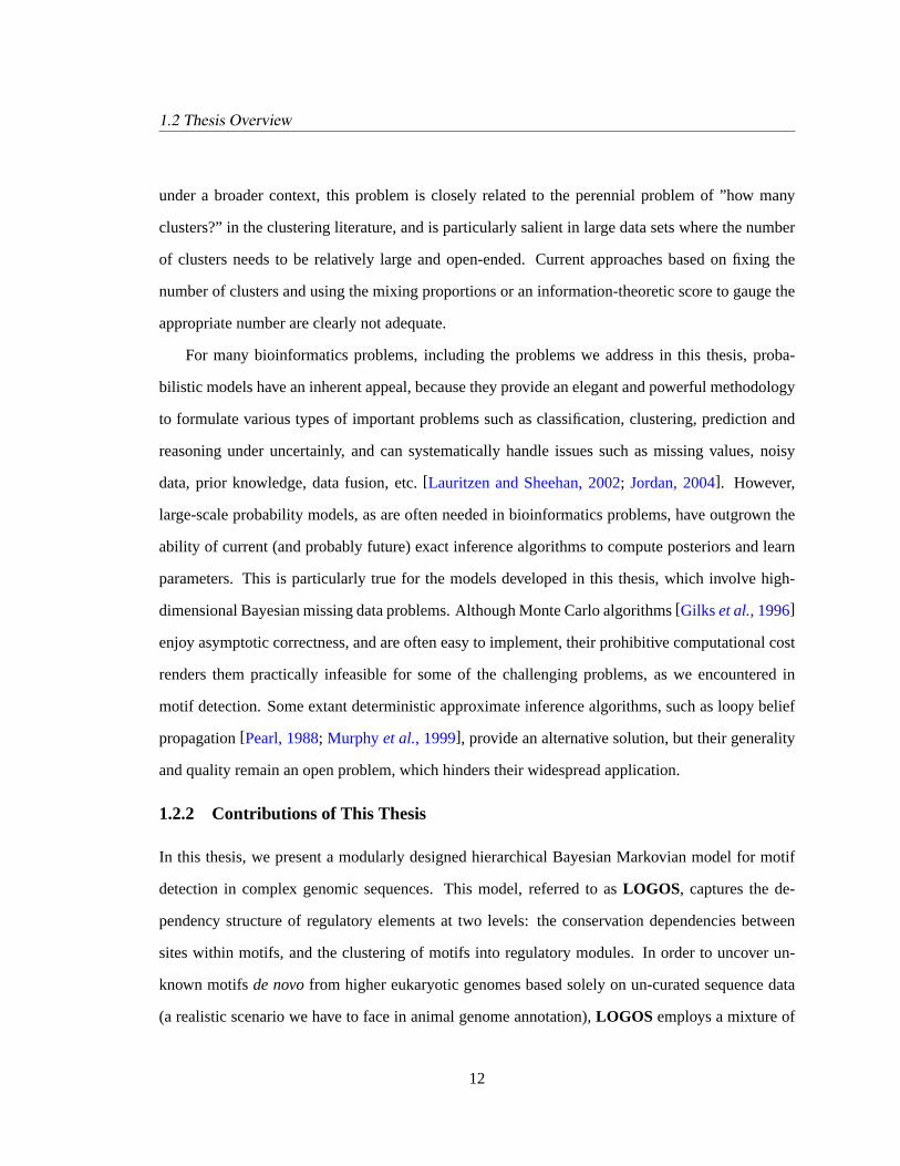
1.2 Thesis Overview
under a broader context, this problem is closely related to the perennial problem of ”how many
clusters?” in the clustering literature, and is particularly salient in large data sets where the number
of clusters needs to be relatively large and open-ended. Current approaches based on fixing the
number of clusters and using the mixing proportions or an information-theoretic score to gauge the
appropriate number are clearly not adequate.
For many bioinformatics problems, including the problems we address in this thesis, proba-
bilistic models have an inherent appeal, because they provide an elegant and powerful methodology
to formulate various types of important problems such as classification, clustering, prediction and
reasoning under uncertainly, and can systematically handle issues such as missing values, noisy
data, prior knowledge, data fusion, etc.[Lauritzen and Sheehan, 2002; Jordan, 2004]. However,
large-scale probability models, as are often needed in bioinformatics problems, have outgrown the
ability of current (and probably future) exact inference algorithms to compute posteriors and learn
parameters. This is particularly true for the models developed in this thesis, which involve high-
dimensional Bayesian missing data problems. Although Monte Carlo algorithms[Gilks et al., 1996]
enjoy asymptotic correctness, and are often easy to implement, their prohibitive computational cost
renders them practically infeasible for some of the challenging problems, as we encountered in
motif detection. Some extant deterministic approximate inference algorithms, such as loopy belief
propagation[Pearl, 1988; Murphy et al., 1999], provide an alternative solution, but their generality
and quality remain an open problem, which hinders their widespread application.
1.2.2 Contributions of This Thesis
In this thesis, we present a modularly designed hierarchical Bayesian Markovian model for motif
detection in complex genomic sequences. This model, referred to asLOGOS, captures the de-
pendency structure of regulatory elements at two levels: the conservation dependencies between
sites within motifs, and the clustering of motifs into regulatory modules. In order to uncover un-
known motifsde novofrom higher eukaryotic genomes based solely on un-curated sequence data
(a realistic scenario we have to face in animal genome annotation),LOGOS employs a mixture of
12
1.2 Thesis Overview
profile motif models, which can be trained on biologically identified motifs categorized according
to protein-binding mechanisms and which can serve as a structured Bayesian prior for a probabilis-
tic motif representation. Such a model biases the likelihoods of nucleotide strings toward those
corresponding to biologically meaningful motifs rather than trivial patterns recurring in the ge-
nomic sequence, but does so withouta priori committing to any specific consensus sequences. To
our knowledge, this is the first model that enablesde novomotif detection to benefit from prior
knowledge of biologically identified motifs, and classifies motifs based on protein binding mecha-
nisms. To model the locational organization of motifs in the genome,LOGOS also uses a hidden
Markov model (HMM) to encode the syntactic rules of motif dependencies, with model parameters
smoothed under empirical Bayesian priors. Using the graphical model formalism, the aforemen-
tioned model ingredients addressing different aspects of motif properties can be integrated into a
composite joint probabilistic model. The modular architecture ofLOGOS manifests a principled
framework for developing, extending and computing expressive biopolymer sequence models.
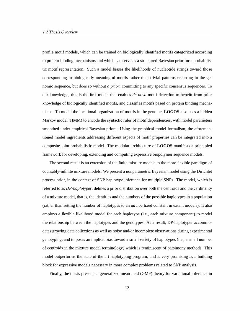
The second result is an extension of the finite mixture models to the more flexible paradigm of
countably-infinite mixture models. We present a nonparametric Bayesian model using the Dirichlet
process prior, in the context of SNP haplotype inference for multiple SNPs. The model, which is
referred to asDP-haplotyper, defines a prior distribution over both the centroids and the cardinality
of a mixture model, that is, the identities and the numbers of the possible haplotypes in a population
(rather than setting the number of haplotypes to anad hocfixed constant in extant models). It also
employs a flexible likelihood model for each haplotype (i.e., each mixture component) to model
the relationship between the haplotypes and the genotypes. As a result, DP-haplotyper accommo-
dates growing data collections as well as noisy and/or incomplete observations during experimental
genotyping, and imposes an implicit bias toward a small variety of haplotypes (i.e., a small number
of centroids in the mixture model terminology) which is reminiscent of parsimony methods. This
model outperforms the state-of-the-art haplotyping program, and is very promising as a building
block for expressive models necessary in more complex problems related to SNP analysis.
Finally, the thesis presents a generalized mean field (GMF) theory for variational inference in
13

1.2 Thesis Overview
exponential family graphical models (to be defined in the sequel). A GMF method uses a fam-
ily of tractable distributions defined on arbitrary disjoint model decompositions to approximate an
intractable distribution, and solves the optimal approximation using a generic message passage pro-
cedure provably convergent to globally consistent fixed points of marginals and leading to a lower
bound on the likelihood of observed data under the distribution. This framework generalizes several
previous studies on model-specific structured variational approximation, yet specializes a previous
study suggesting non-disjoint model decompositions, and appears to strike the right balance be-
tween quality of approximation and computational complexity. This algorithm has been used as
the main inference engine for motif detection using theLOGOS model. The thesis also shows that
the task of model decomposition, which is a prerequisite for the GMF algorithm, can be automated
and optimized using graph partitioning; it demonstrates the empirical superiority of a minimal cut
over other partition schemes, as well as giving theoretical justifications. This combination of GMF
inference with combinatorial optimization represents an initial foray into the development of a truly
turnkey algorithm for distributed approximate inference with bounded performance.
1.2.3 Importance for Bioinformatics, Computer Science and Statistics
The immediate use of these models and algorithms is in allowing us to develop software for solving
certain long-standing computational genomics problems, specifically, motif detection and haplo-
type inference, under realistic and complex biological contexts, with noisy and incomplete mea-
surements, and in light of empirical prior knowledge as well as theoretical insight from biological
literature.
Biological systems are intrinsically complex and stochastic. In recognition of this, we have
strived to develop large-scale mathematical models using principles of probability theory, graph
theory and information theory to capture and appropriately handle these issues. It is our belief
that the lack of mathematical sophistication in many extant bioinformatics models and programs is
a concession to computational complexity, rather than a reflection of the biological reality of the
systems or mechanisms under study. As a step toward dealing with these realities, this thesis also
14

1.2 Thesis Overview
concentrates on exploring computational techniques that can reliably and efficiently solve challeng-
ing large-scale probabilistic models.
Throughout the thesis, the formalism of probabilistic graphical models has been used to con-
struct problem-specific Bayesian models, and guide the implementation of computational algo-
rithms for inference and learning in solving the associated computational biology problem. The
longer term value of this thesis and the most important idea from it, we would hope, is that, in
certain problem domains, one can use probabilistic graphical models from beginning to end as a
general-purpose modeling language to systematically, modularly, and formally build large-scale
models for a complex domain in adivide-and-conquerand bottom-up fashion, avoiding being en-
tangled in the immensely complex and often messy details one has to face in these domains; and
to exploit the availability of general-purpose inference and learning algorithms for graphical mod-
els. As you proceed, the creation of theLOGOS model from theMotifPrototyperandCisModuler
models, and the elaboration ofPedi-haplotyperfrom the basicDP-haplotyperhopefully serve as
motivating examples.
We would particularly like to point out that, when pursuing probabilistic (in particular, Bayesian)
approaches to complicated statistical problems, such as those in the biological domain, it is helpful,
conceptually, to distinguish two separate issues[Stephens and Donnelly, 2003]:
• Themodel (e.g., prior distribution or likelihood function) for the quantities of interest. Exam-
ples (detailed shortly in the technical section) include, special prior models for thepositional
weight matricesof motifs, or for theancestral haplotype templatesof individual haplotypes.
For a given data set, different model assumptions will in general lead to different posterior
distributions and hence to different estimates.
• Thecomputational algorithm used. For challenging problems, including the ones addressed
in this thesis, the posterior distribution cannot be calculated exactly. Instead, computational
methods — such as a variational inference algorithm, or Monte Carlo algorithms — are used
to approximate it. Different computational tricks, or different settings of the “free knobs” in
15

1.2 Thesis Overview
the algorithms (e.g., number of iterations, convergence test, etc.), will change the quality of
the approximation to the true posterior.
Not separating these two aspects in the face of a complex problem can be counter-productive. For
example, it is not unusual to see summary sentences or listings like “we compare our algorithm
TIGERwith the extant algorithmsCAT, EM, the Gibbs sampler, and the hidden Markov model ...”,
which is technically confusing and misleading, and strictly speaking, formally inappropriate. It ob-
scures the technical ingredients of each algorithm, and conceals possible distinctions (or very often,
lack of technical distinctions) between different algorithms—be it a model distinction, an algorith-
mic distinction for computation, or a distinction in the implementation. For instance, algorithm
“TIGER” may also employ a Gibbs sampling algorithm for computation, and the “EM” and “Gibbs
sampler” may have adopted the same probabilistic model. This blurring can cause unnecessary
confusion when analyzing different models and possible duplication of previous work, and makes
it difficult for practitioners or end-users to pick the appropriate algorithm for a certain task, and
for developers to identify technical aspects subject to improvement. In this thesis, we intentionally
make explicit these two aspects of computational probabilistic methodology in the exposition of
existing and new models and algorithms.
The main theme of this thesis is the application of statistical machine learning approaches to
computational biology. However, computational biology is not about simple matching between
textbook algorithms and biological datasets. Close interactions between well-designed biological
experiments and elegant yet realistic formulation of the mathematical models, as well as the de-
velopment of efficient algorithms, are all essential to computational biology research. This thesis
attempts to reflect the intimate interactions between biological concepts, mathematical formalisms,
and computational algorithms, via an exposition that starts from highly problem-specific modeling
efforts, followed by generalizations and combinations thereof, and eventually motivates an attempt
to develop a generic computation technique. We believe that progress in the fields of machine learn-
ing and in biological research can be synergistic. Insights gained from theoretical and algorithmic
research in machine learning can bring a new perspective and tools for studying biological objects,
16

1.3 Technical Results of This Thesis
and can foster new applications. On the other hand, biological research, facing systems of immense
complexity and stochasticity rarely encountered elsewhere, challenges advanced mathematical and
computational techniques for analysis and interpretation, and could lead to new developments that
find broader application in fields outside biology that involve predictive understanding, learning and
reasoning under uncertainty.
1.3 Technical Results of This Thesis
1.3.1 A Modular Parametric Bayesian Model for Transcriptional Regulatory Se-quences
Most conventional motif models lack a clean formalism for imposing useful controls over where to
search for motifs (hence, all regions are taken as equally likely to harbor motifs) and what substring
patterns are preferred over others as candidate motifs (therefore, all recurring substring patterns are
equally likely to be accepted as functionally meaningful motifs). In Chapter 2, we propose a princi-
pled framework for introducing such controls for motif modeling. The goal is to develop a formal-
ism that is expressive (in terms of being able to capture the internal structures, organizational rules,
and other properties of motifs, and readily incorporating prior knowledge about these properties
from biological literature), yet mathematically and algorithmically transparent and well-structured,
hence simplifying model construction, computation and extension. Based on the product rule of the
joint probability in the graphical model formalism, we outline the formal architecture of a modular
motif model with the following three components: thelocal alignment model, which captures the
intrinsic properties within motifs, including characteristic position weight matrices (PWMs) and
site dependencies; theglobal distribution model, which models the frequencies of different motifs
and the dependencies between motif occurrences in a sequence; and thebackground model, which
defines the distribution of non-motif nucleotide sequences. The model components can be designed
separately, and then fused into a consistent, more expressive joint model.
17

1.3 Technical Results of This Thesis
1.3.1.1 Profile Bayesian models for motif sequence pattern
It is well known that the DNA-binding domains of gene-regulatory proteins fall into several distinc-
tive classes, such as the zinc-finger class or the helix-turn-helix class. This classification strongly
suggests that different motif patterns with different consensus sequences may share some local
structural regularities intrinsic to a family of different motifs corresponding to a specific class of
DNA-binding proteins.
In Section§2.4, we address the problem of modeling generic features ofstructurally but not
textuallyrelated DNA motifs, that is, motifs whose consensus sequences are entirely different, but
nevertheless share “meta-sequence features” reflecting similarities in the DNA binding domains of
their associated protein recognizers. We present MotifPrototyper, a profile hidden Markov Dirichlet-
multinomial (HMDM) model that is able to capture regularities of thenucleotide-distribution pro-
totypesand thesite-conservation couplingstypical to a particular family of motifs that correspond
to regulatory proteins with similar types of structural signatures in their DNA binding domains.
Central to this framework is the idea of formulating a profile motif model as a family-specific struc-
tured Bayesian prior model for the PWMs of motifs belonging to the family being modeled, thereby
relating these motif patterns at themeta-sequence level.
The HMDM model assumes that positional dependencies within a motif are induced at a higher
level among a finite number of informative Dirichlet priors, rather than directly between the position-
specific distributions (which are generally set to be multinomials) of the nucleotides of the sites
inside a motif. Under this framework, one can explicitly capture meta-sequence features, such
as different conservation patterns of nucleotide distribution (e.g., beinghomogeneousor heteroge-
neous), and the 1st-order Markov dependencies of such patterns between adjacent sites. In general,
the HMDM model can be used to formally encode prior knowledge about the intrinsic structure of a
family of different motifs sharing meta-sequence features, by learning the parameters of the model
from experimentally identified motifs of the family. This can be done by using a stochastic EM al-
gorithm to compute the empirical Bayes estimate of the parameters. The result is a family-specific
Bayesian profile model that implicitly encodes meta-sequence features shared in this family.
18

1.3 Technical Results of This Thesis
We then show how the family-specific profile HMDMs, or MotifPrototypers, can be used to
classify aligned multiple instances of motifs into different classes each corresponding to a certain
class of DNA-binding proteins; and most importantly, how a mixture model built on top of multiple
profile models can facilitate a Bayesian estimation of the PWM of a novel motif. The Bayesian
estimation approach connects biologically identified motifs in the database to previously unknown
motifs in a statistically consistent way (which is not possible under the single-motif-based repre-
sentations described previously) and turnsde novomotif detection, a task conventionally cast as an
unsupervisedlearning problem, into asemi-unsupervisedlearning problem that makes substantial
use of existing biological knowledge.
A recent paper by Barashet al. proposes several expressive Bayesian network representations
(e.g., tree network, mixture of trees, etc.) for motifs, which are also intended for modeling de-
pendencies between motif sites[Barashet al., 2003]. An important difference between these two
approaches is that, in Barash’s Bayesian network representations, the site-dependencies are modeled
directly at the level of site-specific nucleotide distributions in a “sequence-context dependent” way;
whereas in the HMDM model, the site-dependencies are modeled at the level of theprior distribu-
tions of the site-specific nucleotide-distributions in a “conservation-context dependent” way. Thus,
Barash’s motif models have one-to-one correspondence with particular motif consensus patterns,
and need to be trained on an one-model-per-motif basis. On the other hand, the HMDM model
corresponds to a generic signature structure at the meta-sequence level; it is not meant to commit
to any specific consensus motif sequence, but aims at generalizing across different motifs bearing
similar conservation structures. In terms of the resulting computational task inde novomotif de-
tection, Barash’s model needs to be estimated in anunsupervisedfashion and makes no use of the
biologically identified motifs in the database, whereas the HMDM model helps to turn the model
estimation task into asemi-unsupervisedlearning problem that draws a connection between novel
motifs to be found and the biologically identified motifs via a shared Bayesian prior, so that the pat-
terns to be found are biased toward biologically more plausible motifs. It is interesting to note that
19

1.3 Technical Results of This Thesis
these two approaches are complementary in that Barash’s models provide a more expressive likeli-
hood model of the motif instances, and the HMDM model can be straightforwardly generalized to
define a prior distribution for these more expressive models (e.g., replacing the Markov chain for
the prototype sequence in the HMDM model with a tree model and/or introducing Dirichlet mixture
priors for the parameters of Barash’s models).
1.3.1.2 Bayesian HMM for motif organization
In complex multi-cellular organisms such as higher eukaryotes, the distribution of motif strings
in the genome often follows a general principle called modular organization. That is, the motifs
that are involved in regulating the expression of a given gene are not distributed uniformly and at
random in the regulatory region of the gene. Instead, they are organized into a series of discrete se-
quence regions calledcis-regulatory modules, each of which controls a distinct aspect of the gene.
Within each module certain combinations of motifs occur with increased frequency; these motifs
are capable of integrating, amplifying, or attenuating multiple regulatory signals via combinatorial
interaction with multiple regulatory proteins. This architecture is somewhat analogous to the gram-
matical rules we use to synthesize natural language from words. A motif detection algorithm that
ignores these syntactic rules often fails to correctly score true signals in a motif-dense region but on
the other hand is sensitive to false positives in the background region.
Taking an approach that has been widely adopted in many language and sequence segmentation
problems, we assume that underlying each sequence of nucleotides is a 1st-order hidden Markov
model, whose realizable state sequences correspond to segmentations of the DNA sequence. For
states corresponding to motif sites, the PWM of the corresponding motif is used to define the emis-
sion probabilities of observed nucleotides. For a non-motif state, it is assumed that probability of
the corresponding nucleotide iskth-order Markovian. What is unique about this specialized HMM
model, which we refer to as CisModuler, is the design of the state space of the hidden variables,
which corresponds to a rich set of possible functional annotations of each position in the transcrip-
tional regulatory sequences; and the state-transition scheme, which encodes the stochastic syntactic
20

1.3 Technical Results of This Thesis
rules of the CRM organizations of motifs known from the literature. Also somewhat novel is that
this model is trained in a semi-unsupervised fashion, from unlabeled sequences under a Bayesian
prior centered around empirical guesses of state transition probabilities. Thus, soft controls over the
distances between motif instances and motif modules, and over their dependencies, can be imposed
based on empirical knowledge from some reasonable sources (e.g., domain experts, literature, etc.),
and, due to the Bayesian approach, are subject to dominance by (rather than over) the evidence
when the study data is abundant.
1.3.1.3 The LOGOS model
A combination of the MotifPrototyper and CisModuler models, using the product rule of joint prob-
ability in a graphical model, leads to a novel Bayesian model that is significantly more expressive
than any extant motif detection model. It is referred to asLOGOS, for integratedLOcal andGlObal
motif Sequence model.2 In LOGOS, the functional annotations of a DNA sequence that determine
the motif locations and modular structures are determined by a CisModuler HMM model; but the
emission probabilities of the motif states, or the PWMs of the motifs, are assumed to be generated
from the MotifPrototyper model or a mixture of MotifPrototypers, whereby prior knowledge re-
garding both global motif organization and local motif structure is incorporated. As in other recent
motif models, the background model used byLOGOS is a local 3rd-order Markov model. Under
the trained prior models,LOGOS performsde novomotif detection in a semi-unsupervised fashion.
Note thatLOGOS defines a very general framework for modeling gene regulatory sequences,
using a modular graphical model. Each module can be designed separately to model different
aspects of the motif properties and can be updated without overhauling the whole model. The
Bayesian missing data problem associated withLOGOS is a challenging computational problem
that cannot be handled by extant exact inference algorithms. Nevertheless, the modular structure
of theLOGOS model motives a divide-and-conquer approach for approximate inference using the
2Not to be confused with ‘logo,’ a graphic representation of an aligned set of biopolymer sequences first introduced byTom Schneider[Schneider and Stephens, 1990] to help in visualizing the consensus and the entropy (or “information”)patterns of monomer frequencies. Alogo is not a motif finding algorithm, but is often used as a way to present motifsvisually.
21

1.3 Technical Results of This Thesis
GMF algorithm (described shortly). GMF essentially coupleslocal exact inference computations
for each submodel ofLOGOS using an iterative procedure, and leads to a variational approximation
to the Bayesian estimation. The theoretical and algorithmic issues of variational inference in general
and of GMF in particular are addressed in Chapter 4.
Thanks to the flexibility of assembling a full motif model with different combinations of sub-
models under theLOGOS framework, several variants of theLOGOS model that differ in model
expressiveness (e.g., MotifPrototyper + CisModuler, PWMs + uniform global model, etc.) are con-
structed to examine the performance gain (or loss) due to different model components. There is
strong evidence that improvements introduced in this thesis on both the local aspect (i.e., Motif-
Prototyper over the independent PWMs) and the global aspect (i.e., CisModuler over the uniform
model) of the motif model improve performance. Due to the lack of a sufficient number of well
annotated human regulatory sequences for model evaluation, validations are primarily conducted
on yeast andDrosophilaDNA sequences. It is evident that on both the regulatory sequences of
yeast and those ofDrosophila—whose sizes and complexity are comparable to that of human—the
LOGOS model outperforms the popular MEME and AlignACE algorithms.
1.3.2 A Non-Parametric Bayesian Model for Single Nucleotide Polymorphisms
The problem of inferring haplotypes from genotypes of single nucleotide polymorphisms can be
formulated as a mixture model, where the mixture components correspond to the haplotypes in
the population. The size of the pool of haplotypes is unknown, and biologically, a parsimonious
bias toward a more compact haplotype reconstruction (i.e., a pool with smaller number of distinct
population haplotypes sufficient for explaining the genotypes) is desired. Thus methods for fitting
the genotype mixture must crucially address the problem of estimating a mixture with an unknown
number of mixture components and the parsimony bias. Chapter 3 presents a Bayesian approach
to this problem based on a nonparametric prior known as theDirichlet process[Ferguson, 1973],
which attempts to provide more explicit control over the number of inferred haplotypes than has
been provided by the statistical methods proposed thus far. The resulting inference algorithm has
22

1.3 Technical Results of This Thesis
commonalities with parsimony-based schemes.
In the setting of finite mixture models, the Dirichlet process—not to be confused with the
Dirichlet distribution—is able to capture uncertainty about the number of mixture components[Es-
cobar and West, 2002]. The basic setup can be explained in terms of an urn model, and a process
that proceeds through data sequentially. Consider an urn which at the outset contains a ball of a
single color. At each step we either draw a ball from the urn, and replace it with two balls of the
same color, or we are given a ball of a new color which we place in the urn, with a parameter
defining the probabilities of these two possibilities. The association of data points to colors defines
a “clustering” of the data. As pointed out byTavare and Ewens[1998], this process is not only a
mathematically convenient model to deal with uncertainty of the cardinality of a mixture model, but
it indeed corresponds to an interesting metaphor of “biological evolution without selection.”
To make the link with Bayesian mixture models, we associate with each color a draw from
the distribution defining the parameters of the mixture components. This process defines aprior
distribution for a mixture model with a random number of components. Multiplying this prior by a
likelihood yields aposterior distribution. In Chapter 5, Markov chain Monte Carlo algorithms are
developed to sample from the posterior distributions associated with Dirichlet process priors.
The usefulness of this framework for the haplotype problem should be clear—using a Dirich-
let process prior we in essence maintain a pool of haplotype candidates that grows as observed
genotypes are processed. The growth is controlled via a parameter in the prior distribution that cor-
responds to the choice of a new color in the urn model, and via the likelihood, which assesses the
match of the new genotype to the available haplotypes. This latter point also manifests an advantage
of the probabilistic formalism in that it is straightforward to elaborate the observation model for the
genotypes to include the possibility of errors. Trading off these errors against the size of the pool of
haplotypes can be gauged in a natural and statistically consistent way. Overall, the Dirichlet process
mixture naturally imposes an implicit bias toward small ancestral pools during inference (reminis-
cent of parsimony methods), and does so in a well-founded statistical framework that permits errors.
We call the this non-parametric Bayesian modelDP-haplotyper.
23
1.3 Technical Results of This Thesis
The state-of-the-art algorithm for haplotype inference is the algorithm known as “PHASE.”
The performance of DP-haplotyper is equivalent to PHASE on the easier phasing problems that we
study, and improves on PHASE for the hardest problem; also DP-haplotyper requires less compu-
tation time. It also provides an upgrade path to models that permit recombination and incorporate
pedigrees as we outline in section§3.3, and can potentially generalize to linkage analysis and other
population genetics problems. Thus, DP-haplotyper serves as a promising building block for more
expressive models necessary for more complex problems.
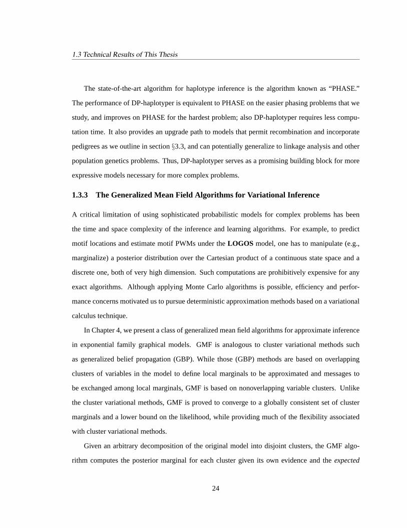
1.3.3 The Generalized Mean Field Algorithms for Variational Inference
A critical limitation of using sophisticated probabilistic models for complex problems has been
the time and space complexity of the inference and learning algorithms. For example, to predict
motif locations and estimate motif PWMs under theLOGOS model, one has to manipulate (e.g.,
marginalize) a posterior distribution over the Cartesian product of a continuous state space and a
discrete one, both of very high dimension. Such computations are prohibitively expensive for any
exact algorithms. Although applying Monte Carlo algorithms is possible, efficiency and perfor-
mance concerns motivated us to pursue deterministic approximation methods based on a variational
calculus technique.
In Chapter 4, we present a class of generalized mean field algorithms for approximate inference
in exponential family graphical models. GMF is analogous to cluster variational methods such
as generalized belief propagation (GBP). While those (GBP) methods are based on overlapping
clusters of variables in the model to define local marginals to be approximated and messages to
be exchanged among local marginals, GMF is based on nonoverlapping variable clusters. Unlike
the cluster variational methods, GMF is proved to converge to a globally consistent set of cluster
marginals and a lower bound on the likelihood, while providing much of the flexibility associated
with cluster variational methods.
Given an arbitrary decomposition of the original model into disjoint clusters, the GMF algo-
rithm computes the posterior marginal for each cluster given its own evidence and theexpected
24

1.3 Technical Results of This Thesis
sufficient statistics, obtained from its neighboring clusters, of the variables in the cluster’s Markov
blanket (to be defined in the sequel) — thence referred to as the Markov blanket messages. The al-
gorithm operates in an iterative, message-passing style until a fixed point is reached. We show that
under very general conditions on the nature of the inter-cluster dependencies, the cluster marginals
retain exactly the intra-cluster dependencies of the original model, which means that the inference
problem within each cluster can be solved independently of the other clusters (given the Markov
blanket messages) by any inference method.
One way to understand the algorithm is to consider a situation in which all the Markov blanket
variables of each cluster are observed. In that case, the joint posterior decomposes:
p(xC1, . . . ,xCn |xE) =
∏i
p(xCi|MB(xCi
),xEi,Ci),
whereMB(xCi) denotes the Markov blanket of clusterCi, andxEi,Ci
denotes the evidence node
within clusteri. GMF approximates this situation, using the expected Markov blanket (obtained
from neighboring clusters) instead of an observed Markov blanket and iterating this process to
obtain the best possible “self-consistent” approximation.
In its use of expectations in messages between clusters, GMF resembles the expectation propa-
gation (EP) algorithm[Minka, 2001], but in the basic EP algorithm the messages convey the influ-
ence of only a single variable. In providing a generic variational algorithm that can be applied to a
broad range of models with convergence guarantees, GMF resembles VIBES[Bishopet al., 2003],
whose original version was based on a decomposition into individual variables, and later generalized
to allow more coarse-grained disjoint decompositions similar to what we used for GMF[Bishop and
Winn, 2003]. Thus GMF is a generic algorithm suitable for approximate inference in large, complex
probability models.
Disjoint clusters have another virtue as well, which is explored in the second half of Chapter 4
— they open the door to a role for graph partitioning algorithms in choosing clusters for inference.
We provide a preliminary formal analysis and a thoroughgoing empirical exploration on how to
choose a good partition of the graph automatically using graph partitioning algorithms, so that the
25

1.4 Thesis Organization
entire GMF inference algorithm can be implemented in a fully autonomous way, with little or no
human intervention. We present a theorem that relates the weight of the graph cut to the quality of
the bound of GMF approximation, and study random graphs and a variety of settings of parameter
values. We compare several different kinds of partitioning algorithms empirically and the results
turn out to provide rather clear support for a clustering algorithm based on minimal cut, which is
consistent with implications drawn from the formal analysis.
The combination of GMF inference with graph partitioning based on combinatorial optimiza-
tion make it possible to develop truly turnkey algorithms for distributed approximate inference with
bounded performance.
1.4 Thesis Organization
The thesis stands at the intersection of several areas, namely, computer science, statistics, molecular
biology and genetics, and draws heavily on statistical machine learning, Bayesian statistics, opti-
mization theory, graph theory, and various biology-related sub-areas. Nonetheless, the reader is not
assumed to have a thorough background in any of these areas, but a general knowledge of the basic
concepts and techniques (e.g., discrete and continuous probability, EM algorithms, etc.) and I have
made some effort to make the thesis readable to a general audience in machine learning, statistics,
and computational biology.
Chapters 2-5 present the main contributions in this thesis. Chapters 2, 3, and 4 are self-contained
and can be read separately from the rest, whereas Chapter 5 should be read in the context of Chap-
ters 2 and 3. Chapter 2 describes a modular parametric Bayesian model for motif detection in
complex genomes. Chapter 3 presents a non-parametric Bayesian model for inferring the haplo-
types of SNPs in a population. Chapter 4 presents a generalized mean field theory and algorithm
for variational inference in exponential family graphical models (to be defined in the sequel) and its
application to motif detection using the models developed in Chapter 2. Chapter 5 provides Monte
Carlo algorithms for inferring motifs and haplotypes based on models in Chapters 2 and 3.
Those readers most interested in novel motif detection techniques as well as a detailed overview
26

1.4 Thesis Organization
of extant methods are advised to read Chapter 2 first and then chapter 4 and section 2 of Chapter
5. Those interested in new models for haplotype inference should start with Chapter 3 and continue
to sections 3-5 of Chapter 5. Those interested in approximate inference theory and algorithms are
advised to read Chapter 4, and then Chapter 2 as an instance of large-scale application.
Chapter 6 summarizes the results of this thesis, draws a few conclusions and presents a set of
open questions and directions for further investigation.
Some of the material in this thesis has appeared before in[Xing et al., 2003a; Xing et al., 2003b;
Xing et al., 2004a; Xing et al., 2004c; Xing et al., 2004b; Xing and Karp, 2004].
27
Chapter 2
Modeling Transcriptional RegulatorySequences for Motif Detection— A Parametric Bayesian Approach
Motifs are short recurring string patterns scattered in biopolymer sequences such as DNA and
proteins. The characteristic sequence patterns of motifs and their locations often relate to important
biological functions, such as serving as thecis-elements for gene regulation or as the catalytic sites
for protein activity. The identification of motif sites within biopolymer sequences is an important
task in molecular biology and is essential in advancing our knowledge about biological systems.
It is well known that only a small fraction of the genomic sequences in multi-cellular higher or-
ganisms constitute the protein coding information of the genes (e.g., only 1.5% for human genomes
[Albertset al., 2002]), whereas the rest of the genome, besides playing purely structural roles such
as forming the centromeres and telomeres of the chromosomes, contains a large number of short
DNA motifs that make up the immensely rich codebook of the gene regulation program, known as
the cis-regulatory system[Blackwood and Kadonaga, 1998; Davidson, 2001]. It is believed that
this regulatory program determines the level, location and chronology of gene expression, which
significantly, if not predominantly, contributes to the developmental, morphological and behavioral
diversity of complex organisms[Davidson, 2001].
For proteins, functional specificities are usually realized by the presence of sporadic, but struc-
turally pivotal and/or biochemically reactiveactivity sitesin the amino acid sequences[Lockless
28
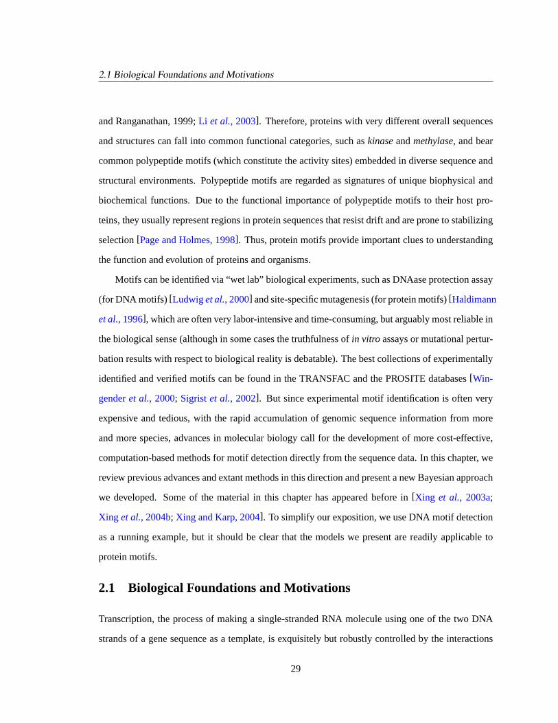
2.1 Biological Foundations and Motivations
and Ranganathan, 1999; Li et al., 2003]. Therefore, proteins with very different overall sequences
and structures can fall into common functional categories, such askinaseandmethylase, and bear
common polypeptide motifs (which constitute the activity sites) embedded in diverse sequence and
structural environments. Polypeptide motifs are regarded as signatures of unique biophysical and
biochemical functions. Due to the functional importance of polypeptide motifs to their host pro-
teins, they usually represent regions in protein sequences that resist drift and are prone to stabilizing
selection[Page and Holmes, 1998]. Thus, protein motifs provide important clues to understanding
the function and evolution of proteins and organisms.
Motifs can be identified via “wet lab” biological experiments, such as DNAase protection assay
(for DNA motifs) [Ludwiget al., 2000] and site-specific mutagenesis (for protein motifs)[Haldimann
et al., 1996], which are often very labor-intensive and time-consuming, but arguably most reliable in
the biological sense (although in some cases the truthfulness ofin vitro assays or mutational pertur-
bation results with respect to biological reality is debatable). The best collections of experimentally
identified and verified motifs can be found in the TRANSFAC and the PROSITE databases[Win-
genderet al., 2000; Sigristet al., 2002]. But since experimental motif identification is often very
expensive and tedious, with the rapid accumulation of genomic sequence information from more
and more species, advances in molecular biology call for the development of more cost-effective,
computation-based methods for motif detection directly from the sequence data. In this chapter, we
review previous advances and extant methods in this direction and present a new Bayesian approach
we developed. Some of the material in this chapter has appeared before in[Xing et al., 2003a;
Xing et al., 2004b; Xing and Karp, 2004]. To simplify our exposition, we use DNA motif detection
as a running example, but it should be clear that the models we present are readily applicable to
protein motifs.
2.1 Biological Foundations and Motivations
Transcription, the process of making a single-stranded RNA molecule using one of the two DNA
strands of a gene sequence as a template, is exquisitely but robustly controlled by the interactions
29
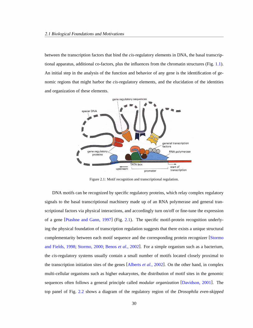
2.1 Biological Foundations and Motivations
between the transcription factors that bind thecis-regulatory elements in DNA, the basal transcrip-
tional apparatus, additional co-factors, plus the influences from the chromatin structures (Fig.1.1).
An initial step in the analysis of the function and behavior of any gene is the identification of ge-
nomic regions that might harbor thecis-regulatory elements, and the elucidation of the identities
and organization of these elements.
Figure 2.1: Motif recognition and transcriptional regulation.
DNA motifs can be recognized by specific regulatory proteins, which relay complex regulatory
signals to the basal transcriptional machinery made up of an RNA polymerase and general tran-
scriptional factors via physical interactions, and accordingly turn on/off or fine-tune the expression
of a gene[Ptashne and Gann, 1997] (Fig. 2.1). The specific motif-protein recognition underly-
ing the physical foundation of transcription regulation suggests that there exists a unique structural
complementarity between each motif sequence and the corresponding protein recognizer[Stormo
and Fields, 1998; Stormo, 2000; Benoset al., 2002]. For a simple organism such as a bacterium,
the cis-regulatory systems usually contain a small number of motifs located closely proximal to
the transcription initiation sites of the genes[Albertset al., 2002]. On the other hand, in complex
multi-cellular organisms such as higher eukaryotes, the distribution of motif sites in the genomic
sequences often follows a general principle calledmodular organization[Davidson, 2001]. The
top panel of Fig.2.2 shows a diagram of the regulatory region of theDrosophila even-skipped
30

2.1 Biological Foundations and Motivations
(eve) gene. This gene is involved in establishing the body segmentation duringDrosophilaem-
bryogenesis by expressing itself in different parts of the early embryo, know as thestripes(mid-
dle panel, Fig.2.2), at different times, to determine the developmental fate of the correspond-
ing stripes[Harding et al., 1989; Goto et al., 1989; Stanojevicet al., 1991; Small et al., 1996;
Sackersonet al., 1999; Fujioka et al., 1999]. For example, the first two stripes shown in Fig.2.2
will grow into the head of the animal, and the third one will become a pair of legs[Gilbert, 2003;
Albertset al., 2002]. As shown in this diagram, the motifs that are involved in regulating the expres-
sion of this gene are not distributed uniformly and at random in the regulatory region of the gene.
Instead, they are organized into a series of discrete sequence regions calledcis-regulatory mod-
ules(or CRMs), each of which controls a distinct aspect of the gene’s expression pattern, namely,
when, in which stripe, and in roughly how many copies it is to be transcribed[Davidson, 2001;
Michelson, 2002]. This general architecture applies to most transcriptional regulatory sequences in
complex organisms, but does not apply to simple uni-cellular biological systems[Davidson, 2001].
stripe 3/7 stripe 2 eve transcript stripe 4/6 stripe 1/5
Figure 2.2: TheDrosophilaCRMs and their roles in early embryogenesis.
As mentioned,in silico motif detection is the task of identifying potential motif patterns from
DNA sequences using a pattern recognition program. However, unlike another pattern recognition
problem on DNA sequences — gene finding — which searches for “macroscopic” entities such
31

2.1 Biological Foundations and Motivations
as genes (or more precisely, exons of the genes) in the genome, motif finding focuses on “micro-
scopic” substring patterns embedded in a long stream of noisy background full of false positive
signals. To the best of our knowledge, most of the biologically verified motifs are very short (i.e.,
about6 ∼ 30 monomers), stochastic (i.e., different instances of the same motif usually differ slightly
in sequence content, as detailed shortly in§2.2.1), and poorly structured (i.e., they contain no sub-
structure bearing universal sequence signatures such as the intron-exon junctions for genes). Thus,
a coarse-grained model, such as a generic HMM that captures a universal intron/exon boundary
signature and the overall nucleotide frequencies of coding sequences, as used in the GENESCAN
program[Burge and Karlin, 1997], is infeasible for detecting small and very diverse motif signals.
More specific models for short sequence patterns, which correspond to regulatory proteins that bear
unique functions, are necessary to represent and search for DNA motifs.
What distinguishes a motif sequence from other random patterns in the background? Besides
the fact that a motif has a recurring consensus polynucleotide pattern, numerous studies of the
biophysical mechanisms of DNA-protein binding underlying thecis-transregulatory interactions
reveal that a typical binding protein (e.g., a transcription factor with helix-turn-helix binding motifs
or tandem zinc-fingers) only interacts with a DNA motif through a few highly specific amino acid-
nucleotide interactions, but is tolerant of variations in other sites[Stryer, 1995; Eisen, 2003]. It is
also well known that for higher eukaryotic organisms, motifs usually cluster into CRMs[Davidson,
2001]. Each CRM consists of a locally enriched battery of motifs occurring in a certain combination
and ordering, capable of enhancing or integrating multiple regulatory signals via concurrent physical
interaction with multiple TFs[Bermanet al., 2002]. The spatial organization of CRMs in the
regulatory regions of the genes is also essential for coordinating gene activities. These features are
not directly reflected in the composition or consensus of a sequence pattern, and therefore can be
referred to asmeta-sequence features.
The meta-sequence features of motif structure and motif organization, which are believed to be
crucial in distinguishing biologically meaningful motifs from a random background or trivial re-
curring patterns, have raised significant challenges to conventional motif-finding algorithms, most
32

2.2 Problem Formulation
of which rely on models that describe motifs only at their sequence level and use simplifying in-
dependence assumptions that decouple potential associations among sites within each single mo-
tif and among multiple instances of motifs[Bailey and Elkan, 1995a; Bussemakeret al., 2000;
Hugheset al., 2000; Liu et al., 2001; Gupta and Liu, 2003]. Therefore, although there is much
success for motif detection on short, well curated bacterial or yeast gene regulatory sequences using
extant methods, generalization to longer, more complex and weakly characterized input sequences
such as those from higher eukaryotic genomes seems less immediate[Papatsenkoet al., 2002;
Rajewskyet al., 2002]. A recent survey by Eisen[2003] raises concerns over the inability of some
contemporary motif models to incorporate biological knowledge of global motif distribution, motif
structure and motif sequence composition.
2.2 Problem Formulation
2.2.1 Motif Representation
To formulate the motif detection problem, we begin with a brief discussion on how to represent a
motif pattern. The representations of motif patterns largely fall into two categories: deterministic
representations, and stochastic representations.
For concreteness, Fig.2.3 shows an example of a stretch of regulatory DNA sequence that
contains instances of multiple motifs. All the sub-strings highlighted with the same color in this
example correspond to the binding sites that can be recognized by the same TF. The simplest way
to represent a motif pattern corresponding to a TF is to consider each motif as a “word” — a de-
terministic substring pattern. However, as shown in Fig.2.3, the instances of a motif are merely
“similar,” but not identical to each other. Thus some flexibility is needed to accommodate dis-
crepancies among instances of the same motif. Usually, biologists record a motif pattern using
a multiple alignmentof all the instances of a motif (Fig.2.3a). An inspection of the alignment
shown in Fig.2.3a suggests that the word “TTTTTATG” may be a reasonable representation of this
motif because it records the most frequent nucleotide at each column of the alignment (although
nucleotides “T” and “A” draw a tie at the 6th column). A word derived from a multiple alignment
33

2.2 Problem Formulation
in this way is called aconsensusof the motif [Stormo, 2000]. In using a consensus sequence to
match additional instances of the motif it represents, some deviations, such ask mismatches with
the consensus (wherek is a small integer compared to the length of the consensus, say,m), are
usually allowed between the instances and the consensus. Aregular expression— in the foregoing
case, “TTTTTXTG”, where “X” means “don’t care” — is another popular deterministic represen-
tation. It can be used to restrict the allowable mismatches to certain positions when matching for
motif instances[Mehldau and Myers, 1993]. There have been several approaches for motif de-
tection directly based on word enumeration[van Heldenet al., 1998; Sinha and Tompa, 2000;
Bussemakeret al., 2000], some of which will be reviewed in the sequel.
(a) (b)
Figure 2.3: A close-up of motif instances and CRMs in aDrosophilasequence.
Alternative to the deterministic representations, due to the stochastic nature of motif patterns,
it is also natural to consider motif instances as samples drawn from a stochastic representation,
which usually corresponds to a generative probabilistic model. For example, a motif can be rep-
resented by aposition weight matrix[Cardon and Stormo, 1992; Hertz and Stormo, 1996], which
records the nucleotide frequencies at each column of the alignment. Pictorially, a motif pattern
can also be represented by asequence logo[Schneider and Stephens, 1990], in which the height
34

2.2 Problem Formulation
of each column corresponds to the degree of conservativeness, measured by the entropy of the nu-
cleotide distribution at a column of the motif alignment; the height of each character in a column
relates to the relative frequency of the respective nucleotides in the corresponding position in the
motif (Fig. 2.3b). With a stochastic motif representation, one can rank the “strength” of matches
of candidate motif instances to a given motif representation with a score that bears probabilistic or
information-theoretic interpretation, such as likelihood or log odds[Stormo, 2000]. In this thesis,
we focus on probabilistic representations of motifs and explore models and algorithms for learning
and prediction under such representations.
2.2.2 Computational Tasks forIn Silico Motif Detection
The term “motif detection”, or “motif finding”, has been heavily loaded in the literature, often
with ambiguous meanings in terms of the exact nature of the intended computational task. To
avoid possible confusion in the forthcoming exposition, in the following we make explicit three
distinct, but related, computational tasks underlying a typical motif detection problem, and assign a
technically unambiguous handle to each.
First, given a set of experimentally identified instances of a certain motif (i.e., all the DNA seg-
ments elucidated from a DNAase-protection assay for a specific DNA-binding regulatory protein),
we call the task of extracting a motif representation, or a motif model, from such a set,motif train-
ing. In machine learning terminology, motif training can be understood as asupervised learning
problem, and the aforementioned set of instances of the motif is called atraining set. As elaborated
in the sequel, depending on the choice of motif representation, different approaches can be used for
motif training, which typically begins with a multiple alignment of all the instances in the training
set, followed by specific procedures to learn the representations, such as a regular expression, a
consensus, or a probabilistic model, from the resulting alignment. In particular, when a motif patten
is represented as a probabilistic model (e.g., the local models in the sequel), motif training boils
down toparameter estimationof the probabilistic model.
Second, given a model or a representation of a known motif, the task of searching for the
35

2.2 Problem Formulation
presence of the sites of this motif in an unannotated set of sequences via computational means is
calledmotif scan. Frequently, generalization to simultaneousmultiple-motif scanis needed. In
many combinatorial motif detection algorithms, motif scan is typically formulated as a “k-m string
matching” problem, that is, finding all substrings of lengthm (i.e.,m-mers, wherem is the length of
the given motif pattern) that has at mostk mismatches with the motif pattern. Accordingly, the motif
patterns to be scanned for are represented by their respective consensus sequences. From a machine
learning point of view, in the simplest case, motif scan can be formulated as a standardclassification
problem for all substrings in the sequences according to a deterministic or probabilistic motif model.
Under a more sophisticated formulation, in which the contextual information and the dependencies
among instances are to be considered, an explicit locational distribution model of motifs (e.g., the
global model in the sequel) can be used, and motif scan can be cast as the problem ofprobabilistic
inferencefor latent random variables in the model that indicate the locations of the motifs.
Finally, given only a set of unannotated sequences potentially containing previously unchar-
acterized motifs (i.e., motifs whose representations are not known), the task of learning the repre-
sentations of these unknown motifs and at the same time locating all the instances of these motifs
in the study sequences is referred to asde novomotif detection. Under a combinatorial setting,
which typically adopts a deterministic representation of a motif pattern,de novomotif detection
often amounts to finding all over-representedm-mers from the sequences, wherem is the length of
the anticipated motifs. Some parameters are needed to qualify a match (e.g., thek in the aforemen-
tionedk-m score) and to determine how many over-represented patterns are to be accepted (e.g.,
a cutoff value for the minimal number of matches)[Papatsenkoet al., 2002]. Under a probabilis-
tic framework, which will be studied in detail in this thesis, one can viewde novomotif detection
as a coupledmissing value inferenceandparameter estimationproblem, often formulated as an
unsupervised learningproblem[Bailey and Elkan, 1995a].
As we will elaborate shortly, besides avoiding possible ambiguities about what one means by
“motif detection”, the foregoing clarification of the computational tasks underlying the motif detec-
tion problem also bodes well for the logic of amodular formulation of thein silico motif detection
36

2.2 Problem Formulation
problem, and adivide-and-conquerstrategy to solve such problems. Just as a quick overview, it is
not difficult to realize that the models (and the algorithms) formotif trainingandmotif scan, respec-
tively, can be viewed as submodels (and subroutines) of the more difficultde novomotif detection
problem in that, computationally,de novomotif detection often amounts to an iterative procedure
(modulo some technical issues regarding how to jump start the iteration, whether it will ever con-
verge, etc.) that alternates between: 1) scanning for instances of a motif using a newly-trained motif
model, and, 2) training an updated motif model using the newly-scanned set of motif instances.
Hence, the full model and the algorithm forde novomotif detection is in essence a combination of
the two models underlying motif scan and motif training, respectively. This modular logic indeed
underlies the two main families of algorithms currently in use forde novomotif detection under
various model settings, namely, expectation-maximization (EM) (e.g.,[Lawrence and Reilly, 1990;
Bailey and Elkan, 1995a]) and Monte Carlo (MC) (e.g.[Lawrenceet al., 1993; Liu et al., 2001]) al-
gorithms. In the sequel, we will adopt this logic to analyze several extant motif models and present
new models and algorithms for motif detection.
2.2.3 General Setting and Notation
Now we introduce the necessary notation for the formal presentation. We denote a regulatory DNA
sequence by a character stringy = (y1, . . . , yT ) ∈ NT , whereN = A,T,C,G denotes the set of
all possible nucleotides (nt) that make up a DNA sequence (for proteins, this set can be redefined
as the set of all possible amino acids). An indicator stringx signals the locations of the motif
occurrences (the range ofx dependents on its specific definition and the model, see later sections
for details). Following biological convention, we denote themulti-alignmentof M instances of a
motif of lengthL by anM × L matrix A, in which eachcolumncorresponds to apositionor site
in the motif. The multi-alignment of all instances of motifk specified by the indicator stringx in
sequencey is denoted byA(k)(x, y). We define acounting matrixh(A(k)) (or h(k)(x, y)) for each
motif alignment, where each columnhl = [hl,1, . . . , hl,4]t is an integer vector with four elements
(the superscriptt denotes vector or matrix transpose), specifying the number of occurrences of
37

2.2 Problem Formulation
each nucleotide at positionl of the motif. (Similarly we define thecounting vectorhbg for the
background sequencey −A, where the somewhat abusive use of the minus sign means excluding
all motif sub-sequences inA from y.) We assume that the nucleotides at positionl of motif k
admit aposition-specific multinomial distribution(PSMD),θ(k)
l =[θ(k)
l,1 , . . . , θ(k)
l,4 ]t. The ordered set
of position-specific multinomial parameters of all positions of motifk, θ(k) = [θ(k)
1 , . . . , θ(k)
L(k) ], is
referred to as aposition weight matrix. It is clear that the counting matrixh(k) corresponds to the
sufficient statisticsfor estimating the PWMθ(k). Formally, the problem of motif training is that of
estimatingθ(k) given the multiple alignmentA(k), for eachk; the problem of motif scan is that of
inferring x(n) given a sequencey(n) andθ(k), ∀n, k; and the problem ofde novomotif detection is
that of inferringx=x(1), . . . , x(N) and estimatingθ=θ(1), . . . , θ(K) simultaneously, given a set
of sequencesy=y(1), . . . , y(N). For simplicity, we omit the superscriptk (motif type index) of
the variableθ and the superscriptn (sequence index) of the variablesx andy wherever it is clear
from the context that we are focusing on a generic motif type or a generic sequence.
2.2.4 The LOGOS Framework: a Modular Formulation
Without loss of generality, assume that the locations of motifs in a DNA sequence, as indicated by
x, are governed by aglobal distribution model p(x|Θg,Mg), and for each type of motif, the nu-
cleotide sequence of all its instances (collected in an alignment matrix) jointly admits alocal align-
ment modelp(A(x, y)|x,Θl,Ml). Further assume that the background non-motif sequences are
modeled by a conditional model,p(y−A(y, x)|x,Θbg,Mbg), where the background nt-distribution
parametersΘbg are usually assumed to be estimateda priori from the entire sequence. The symbols
Θ[·] andM[·] stand for the parameters (e.g., the PWMs) and model classes (e.g., a product multi-
nomial model as described in the sequel) in the respective submodels. Thus, marginalizing over all
possible values of the indicator sequencex, the likelihood of a regulatory sequencey is:
p(y|Θ,M) =∑
x
p(x|Θg,Mg)p(y|x,Θl,Ml,Θbg,Mbg)
=∑
x
p(x|Θg,Mg)p(A|x,Θl,Ml)p(y−A|x,Θbg,Mbg), (2.1)
38

2.2 Problem Formulation
whereA , A(x, y). Note thatΘl here is not necessarily equivalent to the PWMs,θ, of the motifs,
but is a generic symbol for the parameters of a more general model of the aligned motif instances.
(E.g., in the HMDM model to be defined shortly,Θl refers to the hyperparameters that describe a
distribution of PWMs.)
Equation (2.1) makes explicit the modular structure of the probabilistic framework for generic
motif models. The submodelp(x|Θg,Mg) captures properties such as the frequencies of different
motifs, the dependencies between motif occurrences, and the global organization of motif instances.
On the other hand, the submodelp(A|x,Θl,Ml) captures the intrinsic properties within motifs that
can help to improve sensitivity and specificity to genuine motif patterns. Depending on the value
of the latent indicatorxt (e.g., motif or not) at each positiont, yt follows different probabilistic
distributions, such as a specific nucleotide distribution of a particular position inside a motif or a
background distribution. This probabilistic architecture is namedLOGOS, for integratedLOcal
andGlObal motifSequence model.
As equation (2.1) suggests, the specific submodels inLOGOS can be designed separately, and
they are roughly aligned with our specification of the actual computational tasks underlying the
motif detection problem. The local model alone suffices to solve the motif training task, the global
model plus a given set of motif representations suffices to answer the motif scan problem, and their
combination represents thede novomotif detection problem. Recall that the graphical model for-
malism facilitates a modular combination of heterogeneous submodels, using the property of the
product rule of the joint distribution.LOGOS is an instance of such a modeling strategy, and es-
sentially facilitates a bottom-up approach for solving the complexde novomotif detection problem,
by starting from relatively simpler subproblems. This strategy clearly exposes the main technical
issues involved in the motif detection problem, which helps in analyzing existing algorithms and
understanding their merits and limitations. It also enables one to design more sophisticated models
in a piecewise manner to address different aspects of the problem without being overburdened by
the complexity of the overall problem, and to envisage a straightforward path toward solving even
more complex problems, such as joint modeling of motifs and gene expression patterns, by using
39

2.3 An Overview of Related Work
existing or designing new models for each problem (now viewed as subproblems) separately, and
integrating them under the joint graphical model formalism.
2.3 An Overview of Related Work
In the following, we briefly review some representative models for motif detection in the literature.
We will describe these models from theLOGOS point of view, by making explicit the background,
local and global components of the model, even though almost none of the models were originally
constructed and described in such a way, so that the pros and cons of these models can be clearly
understood and compared.
2.3.1 Background Models
2.3.1.1 The models
It is generally assumed that the sequences outside the motifs have diverged sufficiently to be mod-
eled as random background. Thus a simple but very popular model for all the non-motif nucleotides
in the the background sequence is aniid multinomial model:
p(y −A|x,Θbg) =∏t∈B
∏i∈N
[θbg
]I(yt,i) =∏i∈N
[θbg
]hbg,i , (2.2)
whereB is the set of indices of the background positions, andθbg denotes the vector of multinomial
parameters of the background model, which is usually directly computed as the overall nucleotide
frequency distributions of the entire input sequence, assuming that motif instances are sparse in the
sequence and thus would not bias the estimated frequencies[Bailey and Elkan, 1995a; Hugheset
al., 2000; Liu et al., 2001]. (This assumption is somewhat unwarranted in some early literature in
which the input sequences are usually assumed to be sets of100 ∼ 200-mers, each containing, say,
one motif, which suggests a quite significant10% motif coverage! e.g.,[Cardon and Stormo, 1992;
Lawrenceet al., 1993])
Several recent papers have stressed the importance of using a richer background model for the
non-motif sequences[Thijs et al., 2001; Liu et al., 2001; Huanget al., 2004]. In particular, a number
40
2.3 An Overview of Related Work
of higher-order Markov models have been explored by various authors and reportedly contribute to
notable improvements in the performance of motif scan andde novomotif detection. Under a global
kth-order Markov model for non-motif nucleotide sequences, the conditional probability of a single
nucleotidej at sitet is contingent on thek preceding bases following the usual Markov dependency
definition
p(Yt = i|Xt = bg) = p(Yt = i|yt−1, . . . , yt−k) = fi(yt−1, . . . , yt−k).
Thus the probabilities of all the background can be computed by enumerating all(k + 1)-tuples
of nucleotides in the entire sequencey (note that these probabilities need to be computed only
once, and then stored for repeated references during probabilistic inference). The total time for this
operation isO(T ), whereT is the total length of the input sequences. One can also use a local
kth-order Markov model, in which the conditional probability of a nucleotidei at positiont, f ti (·),
is estimated from a local window centered at positiont.
2.3.1.2 The use of background models
As detailed in the sequel, one family of motif scan algorithms seek to score candidate sequence
segments for their similarity to a known motif pattern. The background model plays an important
role in formulating a good scoring function. For example, the standardlikelihood ratio score for
candidate segmentyt,t+L−1 at positionst to t+ L− 1 is computed as follows
rt =p(yt,t+L−1|Θl,Ml)p(yt,t+L−1|Θbg,Mbg)
. (2.3)
A variant of the likelihood ratio score is thelog oddsscore
lt = log rt = log p(yt,t+L−1|Θl,Ml)− log p(yt,t+L−1|Θbg,Mbg). (2.4)
From these two scoring schemes, it is apparent that, even though the motif model, which defines
the probability of a motif segment, is the most important component in these scoring functions, a
good background model will help to improve the contrast of motif to background, and therefore the
discriminating power ofrt or lt at each position.
41

2.3 An Overview of Related Work
Note that while probabilities are used in constructing the scoring functions, the scores them-
selves (e.g., likelihood ratio, log odds) cannot be interpreted statistically. Usually, they will be
compared against anad hoccutoff value to generate computational motif predictions, and choosing
the score cutoff values for each motif and background model is generally difficult. This may have
contributed to the large number of false positive predictions seen in practice. To assess the signifi-
cance for a set of predicted motif instances,Liu et al.[1995] developed a rank test that compares the
prediction results from the study data with those from control data generated by a random shuffle
of the study data. They applied a Wilcoxon signed rank test to the predictions made from paired
(concatenated) study and control data, and obtain ap value of the prediction from the study data
under the rationale that, under the null hypothesis, the motifs are equally likely to be solicited from
either the study or the control sequences.Huanget al. [2004] proposed ap-value based scoring
scheme, which computes the probability that the null (i.e., background) model can achieve a stan-
dard log-likelihood score for a candidate sequence segment at least as high as that of a signal (i.e.,
motif) model defined by PWMs. They developed an exact algorithm based on probability generating
functions to compute thep-value for a generalkth-order Markov background model with respect
to motif models represented by PWMs. The CREME program bySharanet al. [2003] proposed
a number of closed-form statistical scores for assessing the significance of single motif abundance
or abundance of a motif cluster (multiple spatially-close motifs) out of a subregion of a study se-
quence over that of the background sequences. Note that “abundance” (i.e., the number of motif
matches), rather than the score of the matches, is tested for significance in the CREME program, and
it was demonstrated to be a competent method to scan for CRMs in higher eukaryotic transcription
regulatory sequences.
Generally, depending on the choice of grammatical models for global sequence annotation, the
background model can be plugged in as a conditional model for the background state and contribute
to various scoring functions for motif detection. For example, it can be used as an emission model
under a background state in the case of a HMM global model (see§2.5 for details). Rather than
contributing anr or l score, in these cases, the background model will contribute indirectly to the
42

2.3 An Overview of Related Work
posterior probability distribution of the indicator sequencex.
2.3.2 Local Models — for the Consensus and Stochasticity of Motif Sites
A local alignment model attempts to captures the consensus and the accompanied stochasticity of
the set of binding sites (i.e., motif instances) corresponding to a certain TF.
2.3.2.1 Product multinomial model
The position weight matrix introduced in§2.2.3 is the most commonly used representation for a
motif pattern in extant motif detection algorithms[Bailey and Elkan, 1995a; Hugheset al., 2000;
Liu et al., 2001; Frith et al., 2001; Liu et al., 2002; Gupta and Liu, 2003]. Statistically, a PWM can
be used to define aproduct multinomial(PM) model for every observed instance of a motif[Liu
et al., 1995]. Formally, given the PWM,θ = [θ1, θ2, . . . , θL], of a motif, the probability of an
observed instance of this motif, which corresponds to a row in the motif alignment matrixA, say,
Am = [Am,1, Am,2,, . . . , Am,L], is
p(Am|Θl) =L∏
l=1
∏i∈N
[θl,i
]I(Am,l,i). (2.5)
For an alignment ofM motif instances,A = AmMm=1, the joint probability of all motif
instances inA is
p(A|Θl) =M∏
m=1
p(Am|Θl) =L∏
l=1
∏i∈N
[θl,i
]hl,i . (2.6)
Recall thath ≡ hl,i is thenucleotide count matrixassociated with alignmentA, thus,hl,i =∑m I(Am,l, i).
The PM model inherently assumes that the nt-contents of positions within the motif are inde-
pendent of each other. Thus, a PWM only models independent statistical variations with respect to
a consensus pattern of a motif, but ignores potential couplings between positions inside the motif
— a limitation that often weakens its ability to discern genuine instances of a motif from a very
complex background that may harbor random recurring patterns, due to the low signal/noise ratios
reflected in the likelihood-based scores computed from the PM model.
43

2.3 An Overview of Related Work
Given a set of aligned instances of a certain motif (i.e., atraining alignment), under the PM
model, the PWM of this motif can be obtained via maximal likelihood estimation (MLE), which is
equivalent to computing the nt-frequency at each motif position. If the training alignment contains
only a small number of motif instances, MLE tends to lead to a non-robust model (i.e., with a
high variance associated with the estimates of the model parameters), which tends to generalize
poorly to unseen instances of the same motif. For example, if a particular nucleotide does not
appear at a certain position among all the instances in the training alignment, possibly just because
the alignment is too small to be sufficiently representative, then every candidate instance from a
new dataset that bears this nucleotide at this position (but is otherwise highly consistent with the
motif consensus,) will be assigned a zero probability. This artifact is calledoverfittingin statistical
learning, and should be avoided when learning from a small training dataset. In the motif modeling
literature, the most popular remedy is to add to the actual count matrixh a uniformpseudo-count
matrix (i.e., all elements of the matrix are equal)[Lawrenceet al., 1993; Bailey and Elkan, 1994],
which can be regarded as the nt-count from an imaginary set of “motif instances”. The column sum
of the pseudo-count matrix, typically set to 1, can be understood as the total number of “imaginary
motif instances” from which the “count” is obtained. The larger this number is, the more difficult
to override the pseudo-counts with the actual counts from the training data.
Mathematically, incorporating uniform pseudo-counts into the MLE of a PWM is equivalent to
introducing a symmetric Dirichlet prior (AppendixA.1) for the values of each column of the PWM,
and the resulting motif model is also called aproduct Dirichlet (PD) model[Bailey and Elkan,
1995b; Liu et al., 1995]. Note that pseudo-counts or PD models are primarily used for smoothing,
rather than for explicitly incorporating prior knowledge about motifs, and the parameters are chosen
ad hoc.
2.3.2.2 Constrained PM models
Although there are some obvious limitations of PWMs, they have proved to be reasonably effective
in describing the set of sequences bound by a given TF and have shown considerable predictive
44

2.3 An Overview of Related Work
power [Stormo, 2000]. However, in an unsupervisedde novomotif finding scenario where the
PWMs have to be estimatedab initio, the estimated PWMs under the PM model, or even with
pseudo-counts or symmetric Dirichlet priors, are sensitive to noise and random or trivial recurrent
patterns (e.g., poly-N or repetitions of shortk-mers such as CpG islands). Furthermore, the PM
model is unable to capture potential position dependencies inside the motifs.
Various pattern-driven approaches have been developed to handle motifs with specific motif
patterns. For example, in the early Lawrence and Reilly paper[1990], the authors introduced con-
straints on the parameters of the PWM to enforce palindromicity. Frechet al.’s method[1993]
proposed to originate the PWMs from a highly conserved consensus core and then extend the core
in one or both directions. Some of the recent methods providead hocways of allowing motifs to
have two conserved blocks separated by a few background sites, such as splitting a “two-block”
motif into two coupled sub-motifs[Liu et al., 2001; Bailey and Elkan, 1995a]. The fragmentation
model ofLiu et al. [1995] allows an arbitraryL < W positions in an aligned segment of widthW
to constitute the conserved motif sites.
Note that in addition to the nt-frequencies represented by the matrix elements, PWMs can also
provide theinformation content profile[Schneideret al., 1986] of the corresponding motif. The
information content (IC) at a positionl in a motif is given by
Il = log2 |N|+∑i∈N
log2 θl,i, (2.7)
and can be thought as a measure of how conserved positionl is.
Keleset al. [2003] noted that the PWMs describing motifs with very different nt-specificities
can have similar information profiles, and speculated that there is a direct relationship between the
structural footprint of a TF and the information content profile of the corresponding motif. They
developed a method that explicitly enforces nt-biases, e.g., high versus low information contents at
various positions, when computing the MLE of the PWM from samples. They have proposed several
canonical information content patterns, such as the one with aU-shapedcontour, or abell-shaped
contour, to be plausible constraints forde novomotif detection, and have developed a sequential
45

2.3 An Overview of Related Work
quadratic programing method to solve the constrained optimization problem. A constrained EM
algorithm was developed by Kechriset al.[2004] to incorporate similar IC constrains for estimating
motif PWMs.
The IC-constraint approach represents a significant advance in learning local motif models be-
cause it takes into consideration the commonalities shared among motifs of different TFs (with dif-
ferent nt-specificities), and reveals something intrinsic to biologically genuine motifs. However, it
defines a hard constraint that must be respected no matter how many actual motif instances are used
to estimate the PWM, and cannot be overridden when the IC of an abundant novel motif deviates
from the predetermined constraints.
2.3.2.3 Motif Bayesian networks
A recent article by Barashet al. [2003] proposed a family of more sophisticated representations
to capture richer characteristics of motifs. These representations are based on directed probabilis-
tic graphical models, i.e., Bayesian networks. Barashet al. suggested that a mixture of product
multinomial models (MPM),
pMPM (A|Θl) =∑
j
wjpPM (A|θ(j)), (2.8)
wherewj is theweightof thejth mixture component andθ(j) is the PM parameter of thejth mixture
component, can capture potential multi-modalities of the biophysical mechanism underlying the
protein-DNA interaction between a TF and its target motif sites. Under the MPM model, a motif
is characterized by multiple PWMs, each corresponding to a component PM model. Barashet
al. further proposed a tree-based Bayesian network capable of capturing pairwise dependencies
of nucleotide contents between nonadjacent positions within the motif. A natural combination of
the above two models leads to a more expressive model, a mixture of trees, which captures more
complex dependency characteristics of motifs. In a series of experiments with simulated and real
data, Barashet al. showed that these more expressive motif models lead to better likelihood scores
for motifs, and can improve the sensitivity and specificity of motif detection in yeast regulatory
sequences under a simple scenario of motif occurrence (i.e., at most one motif per sequence).
46

2.3 An Overview of Related Work
In principle, it is possible to construct even more expressive models for motifs by systematically
exploiting the power of graphical models, although fitting more complex models reliably demands
more training data. Thus, striking the right balance between expressiveness and complexity remains
an open research problem in motif modeling.
2.3.3 Global Models — for the Genomic Distributions of Motif Sites
The local model of a motif pattern only creates aligned multiple instances of a motif, but does
not complete the generation of the observed sequence set, even with the addition of the background
model. It is necessary to have a set of “rules” that define where and how instances of one or multiple
motifs are embedded in the background sequence so that they can constitute a sort of “language”
or “program” interpretable by the TFs in a liquid solution environment, and in a TF composition
and concentration sensitive manner. In theLOGOS framework, these “rules” are encoded in the
global distribution model for the indicator variable sequencex that can specify the locations and
organization of all motif instances.
2.3.3.1 Theoopsand zoopsmodel
The probabilistic model forde novomotif detection developed by Lawrence and Reilly in their
seminal 1990 paper[Lawrence and Reilly, 1990] assumes that each of theN input DNA sequences
contains exactly one binding site of the same TF. This assumption is an idealization of a scenario in
which a set of “co-regulated” genes are analyzed, and the co-regulation is induced by a single TF
that can bind to a unique motif site present in the regulatory region of each of the regulated genes.
Accordingly, this model is called a “one motif per sequence” (oops) model. Although hardly a
realistic model, the oops model has historical importance (and is still in use in many contemporary
programs) in that it provides a clean abstraction that helps in understanding the motif detection
problem and points out a direction for formulating and upgrading the global model. Formally, let
y(n) = y(n)
t Tnt=1, y(n)
t ∈ N, denote the data of thenth sequence with lengthTn; and letX(n) ∈
1, . . . , Tn − L+ 1 denote the latentaddressvariable of a motif with lengthL in sequencen (the
address of the motif is defined as the position of the most proximal nucleotide in the motif instance,
47

2.3 An Overview of Related Work
w.r.t. the end of the study sequence). The oops model assumes that the location of the (only) motif
in each sequence admits a uniform distribution over all possible positions in the sequence. That is,
p(X(n) = t) =1
Tn − L+ 1. (2.9)
Givenx(n), the oops model assumes that nucleotides at positions not corresponding to the mo-
tif, hence falling into the background, are independently and identically distributed; whereas the
nucleotides of all positions within a motif instance jointly follow a local motif model (e.g., a PM
model as in[Lawrence and Reilly, 1990]). Motif instances in different input sequences are assumed
to be independent and identically distributed. Thus, given the PWMθ of the motif andθbg for the
background, and denoting the nt-count vector of the entire sequencey(n) by h(n), the joint proba-
bility distribution of the observed sequencey(n) and the latent addressesx(n) of the motif therein
is:
p(X(n) = t, y(n)|Θ = θ, θbg) = p(X(n) = t)p(y(n)|X(n) = t,Θ = θ, θbg)
=1
Tn − L+ 1
L−1∏l=0
∏j∈N
[θl,j
]I(y(n)t+l,j) ·
∏j∈N
[θbg,j
]h(n)bg,j ,
=1
Tn − L+ 1
L−1∏l=0
∏j∈N
[ θl,j
θbg,j
]I(y(n)t+l,j) ·
∏j∈N
[θbg,j
]h(n)j ,(2.10)
which leads to the following posterior distribution of the latent variableX(n):
p(X(n) = t|y(n),Θ) =
∏L−1l=0
∏j∈N
[θl,j/θbg,j
]I(y(n)t+l,j)∑T−L+1
t′=1
∏L−1l=0
∏j∈N
[θl,j/θbg,j
]I(y(n)
t′+l,j). (2.11)
Thus, the probability of positiont being a motif start address is proportional to the likelihood ratio
of a sub-sequence of lengthL started att being a motif sequence with respect to its probability of
being a background sequence, which is exactly the likelihood ratio score we described in§2.3.1.
A simple extension of the oops model is thezoopsmodel, for “zero or one motif per sequence”,
adopted by Bailey and Elkan[1994] in their precursor of the MEME algorithm. As the name
suggests, this model is slightly more flexible than oops. For each sequence, zoops introduces an
indicator variableZn ∈ 0, 1, which indicates the presence (Zn = 1) or absence (Zn = 0) of
48

2.3 An Overview of Related Work
a motif instance in sequencen. The prior distribution ofZn can be defined as a simple Bernoulli
distribution,Zn ∼ Ber(α, 1 − α), and the indicator is independent and identically distributed for
each sequence. Under this setting, the conditional likelihood of the observed sequence is
p(y(n)|X(n) = t, Zn = 1,Θ = θ, θ0) =1
Tn − L+ 1
L−1∏l=0
∏j∈N
[ θl,j
θ0,j
]I(y(n)t+l,j) ·
∏j∈N
[θ0,j
]h(n)j ,
p(y(n)|Zn = 0,Θ = θ, θ0) =∏j∈N
[θ0,j
]h(n)j . (2.12)
Thus the probability of having a motif at positiont of sequencen is regularized by the prior
probability of motif presence,
p(X(n) = t, Zn = 1|y(n),Θ) =p(y(n)|X(n) = t, Zn = 1,Θ)p(X(n) = t)p(Zn = 1)
p(y(n)|Θ)
=
∏L−1l=0
∏j∈N
[θl,j/θ0,j
]I(y(n)t+l,j)∑T−L+1
t′=1
∏L−1l=0
∏j∈N
[θl,j/θ0,j
]I(y(n)
t′+l,j) + (1−α)(Tn−L+1)
α
.
(2.13)
2.3.3.2 General uniform and independent models
Essentially, both the oops and zoops models areuniform (over all possible positions in a study
sequence) andindependent(between motif instances and between study sequences) global models,
or in short, UI models, which are intended for simple and idealized motif-bearing sequences. It
is straightforward to generalize the baseline UI model to handle slightly more complex scenarios,
such as multiple motifs per sequence. For example, rather than allowing at most one motif per
sequence, some motif detection algorithms assume that a fixed number of motif instances can be
present independently with uniform probability at all possible locations in a sequence[Bailey and
Elkan, 1995a]. That is, the joint distribution of the addresses of, say,M motif instances in a study
sequencen, x(n) = x(n)
1 , . . . , x(n)
M , can be written asp(x(n)) =∏
M
m=1p(x(n)
m ), wherep(x(n)m =t)
is the prior probability of themth motif instance at locationt in sequencen, in this case, a uniform
distribution over all validt’s and the same for allm = 1, . . . ,M . It can be shown that the marginal
posterior probability of any one of the addresses under this setting,p(x(n)m |y(n),Θ), is proportional
49

2.3 An Overview of Related Work
to the likelihood ratio score of each sequence position (i.e., Eq. (2.11)), and the joint posterior of
all addresses is the product of the posterior probabilities of individual addresses,p(x(n)|y(n),Θ) =∏m p(x(n)
m |y(n),Θ). This model is called anM motifs per sequencemodel (mops), and is used in
various contemporary algorithms, such as MEME. A drawback of this approach is the requirement
of a prespecified number of motif instances. An inaccurately supplied number will lead to either
significant false positives, or false negatives, or both. Also problematic is that the mops model
ignores possible constraints on co-occurrences of motifs.
A slightly more sophisticated model for multiple motif locations per sequence is aniid Bernoulli
indicator model[Liu et al., 1995], which assumes that each host sequencey is associated with
a binary indicator sequence,x = (x1, . . . , xT ), xt ∈ 0, 1, where0 signals background and1
signals a motif starting at positiont; eachXt is an independent Bernoulli random variable,xt ∼
Ber(α); and the Bernoulli parameter[α, 1 − α] follows a Beta prior. This model is essentially a
clustering model for all possibleL-mers of the sequences, allowing anyL-mer to be either a motif
or background.
Under both the mops and Bernoulli indicator models, there is no formalmodel constraintto pre-
vent having overlapping motif instances. Although overlapping motifs are possible in real genomic
sequences, the possibility of overloading every sequence position with multiple motif instances is
not desirable. Therefore, in practice, both models are augmented heuristically with an artificialnon-
overlapping constraint, which requires that noL-mer is allowed to harbor, say, more thanl motif
start positions, where1 < l ≤ L. This constraint is enforced by either rescaling the joint posterior
p(x|y) (as in an EM-based inference strategy for MEME[Bailey and Elkan, 1995a]), or simply
throwing away any overlapping motif samples (when using a Gibbs-sampling-based inference strat-
egy [Liu et al., 1995]). Nevertheless, these heuristics may result in inconsistencies between the
computed motif distribution and the one defined by the model, and incur a sizable overhead due to
wasteful computations.
Despite their simplicity and some unwarranted heuristic assumptions, UI models appear to be
competent in motif scan andde novomotif detection for bacterial or simple yeast sequence sets, in
50

2.3 An Overview of Related Work
which the input sequences are usually short and enriched (e.g., pre-screened according to mRNA
co-expression). But some recent studies including our own experiments suggest that the correctness
of motif detection based on the UI assumptions starts to break down for less well pre-screened input
sequences or for those with clustered motif occurrences, such as theDrosophilagene regulatory
sequences[Bermanet al., 2002]. Higher eukaryotic genomes indeed present a challenge to the
computational identification of motifs because of their long non-coding regions and large number
of repeat elements.
2.3.3.3 The dictionary model
Bussemakeret al. proposed a novel formulation of the motif-finding problem, which is based on
word segmentation and dictionary construction[Bussemakeret al., 2000]. In their MobyDick algo-
rithm, they view the regulatory DNA sequences as sentences written in an unknown language built
from an alphabet of 4 characters (i.e.,N = A, T,G,C as defined previously), with no separators
between words. (In fact, some major human languages, such as Chinese and Japanese, are of this
kind, although using a much larger alphabet, e.g.,> 104, for Chinese.) Under this framework,
the motif-finding problem can be cast as finding over-represented words from consecutive lists of
characters, and the algorithm boils down to an iterative procedure alternating between building up a
dictionary of words and estimating the values of parameters of a language model from a given word
segmentation (e.g., word frequencies), and finding the optimum segmentation of the sequence given
the dictionary and the language model. From theLOGOS point of view, the noise-less “words”
in the motif dictionary represent a deterministic local model of the motifs. Consequently, a de-
generate motif pattern could be represented by several similar words during the construction of the
dictionary, which can be merged into a consensus afterward. The “language model” adopted by the
MobyDick algorithm consists of an array of word-usage probabilities and an assemblage scheme
(analogous to a “grammar” of word usage in natural language) of the sequences, which manifests
a novel global model for motif distribution, and largely contributes to the strength of the Moby-
Dick algorithm. This language model assumes that each word is associated with a frequency of its
51

2.3 An Overview of Related Work
usage, and a sequence is realized by a non-overlapping concatenation of words sampled according
to their frequency (which implicitly assumes that the background model corresponds to a large set
of short words with low frequencies). The conditional probability of a sequence given a possible
segmentation specified by indicator sequencex under this setting is
p(y|x) =1Z
∏k
ρnk(x)k , (2.14)
whereρk denotes the frequency of wordk, nk(x) denotes the counts of wordk in y under segmen-
tationx, andZ is a normalization constant (i.e., the partition function).
Some key advantages of this global model are its emphasis on combinatorial analysis of a large
set of potential motifs (up to all possible substring patterns ofk-mers allowable by the computing
resource), and an explicit non-overlapping constraint on individual substrings induced by the word
segmentation. Since the number of segmentations of an average-sized sequence could be huge,
computing the partition functionZ of Eq. (2.14) and various derivatives ofZ is non-trivial, and a
dynamic programming algorithm is developed.
To account for the sequence variations of each motif pattern, in a recent paper,Gupta and
Liu [2003] extended the MobyDick model to a stochastic dictionary (SD) model by replacing the
words in the dictionary with PWMs. From aLOGOS point of view, this corresponds to upgrading
the local model of MobyDick from deterministic words to PM. Letx denote a word-segmentation
of sequence sety, H = h(1), . . . , h(D) denote the set of nt-count matrices for all the words (with
PWMsθ(k)Dk=1) due to segmentationx, andN = n1, . . . , nD denote the counts of word oc-
currences. The complete data likelihood given all PWMsθ and the word usage probabilitiesρ
is:
p(N ,H, x|θ, ρ) ∝D∏
k=1
ρnkk
Lk∏l=1
4∏j=1
[θ(k)
l,j ]h(k)l,j . (2.15)
Essentially, SD adopts a specific distribution model for motif instances which treats the ob-
served sequences as being generated by concatenating words independently drawn from a dictio-
nary according to a vector of word usage probabilities, while retaining the PM model for aligned
52

2.3 An Overview of Related Work
motif instances. This is equivalent to upgrading the UI model to a finite mixture model with mixture
components being all the PWMs in the dictionary weighted by the word usage probabilities. Due
to this nice connection to the conventional motif models, many of the modeling ideas originally
introduced to the conventional models were readily adaptable to the SD model, such as smoothing
the model with conjugate priors for the PWM and word usage probabilities, and an extension al-
lowing stochastic insertions and deletions in motif instances (to model gaped motifs.) Since in the
model SD, the motif indicatorX is defined as a segmentation variable, with a huge state space that
prohibits exact inference, inference and parameter estimation are performed using a Monte Carlo
procedure.
2.3.3.4 The sliding-window approaches
The uniform and independent models and the word-segmentation models described above treat all
regions in a sequence equally, ignoring potential coupling of multiple motif instances in any sub-
regions of the sequence. However, as discussed in the introduction, in higher eukaryotic genomes,
motifs are often organized intocis-regulatory modules, in which the motif occurrences tend to be
significantly enriched compared to the background region, and encode some complex combinatorial
signals. This architecture implies that during motif scan, locally clustered weak motif signals may
need to be treated with higher weights because they may suggest co-occurring weak binding sites in
a CRM; whereas an occasional seemingly strong signal out of a long stretch of sequence with low
score may need to be weighted lower because it may be just a spurious signal in the background.
The sliding-window method is one of the most popular approaches for motif and CRM predic-
tion that tries to incorporate the aforementioned architectural features of motif distribution[Halfon
et al., 2002; Papatsenkoet al., 2002; Rajewskyet al., 2002; Nazina and Papatsenko, 2004]. Typ-
ically, a sliding-window method counts the number of matches of some minimal strength to given
motif patterns within a certain window of DNA sequences using certain scoring functions, such as a
likelihood ratio (when the motifs are represented by PWMs[Sharanet al., 2003]) or thek-m score
53
2.3 An Overview of Related Work
(when the motifs are represented by deterministic words)[Papatsenkoet al., 2002]. From a mod-
eling point of view, this family of algorithms assumes that motifs are uniformly and independently
distributed only within each window. Anad hocwindow size needs to be specified and careful
statistical analysis of matching strength is required to determine a good cutoff or scoring scheme.
The CREME algorithm[Sharanet al., 2003] uses a comparative genomic approach to identify
the putative CRM regions (thus avoiding the need to specify the window size), and a number of
sophisticated scoring functions were proposed to measure the statistical significance of local en-
richment of candidate motif matches in these regions.
Nazina and Papatsenko[2004] addressed the issue of compensating the matching scores for
co-occurring weak motif sites using an updatable “word-frequency” measure, which leads to higher
scores for motifs occurring more frequently within a window of a given size. This approach is anal-
ogous to a MobyDick model applied to each window. A sliding-window version of the stochastic
dictionary model was used by Rajewskyet al. in their Ahab/Argos program[Rajewskyet al., 2002].
2.3.3.5 The hidden Markov model
Another way to handle sequences bearing rich motif content and architecture is to explicitly model
the organizations of the motifs using a stochastic sequential model that encodes “rules” to generate
such motif organizations. For example, the program Cister[Frith et al., 2001] assumes that the
indicator sequence of a study sequence,x, admits a 1st-order Markov model,
p(x) = p(x1)T∏
t=2
p(xt|xt−1), (2.16)
whose state space consists of background states and motif states. The occurrences of motifs and
CRMs are induced by an emission model,p(yt|xt), which generates state-specific nucleotide out-
puts belonging to a motif or the background. Note that the stochastic rules of the motif organization,
such as how often a CRM appears, how long a CRM tends to be, and how often motifs appear in a
CRM, are encoded in the state-transition probabilities of these indicator variables. Since the indica-
torsx are not observed, this is a classical hidden Markov model with discrete output.
54

2.3 An Overview of Related Work
An HMM for motif scan renders both the window size and the score cutoff unnecessary, and
takes into account not only the strengths of motif matches, but also the spatial distances between
matches (arguably more informative than co-occurrences within a window). The hidden Markov
model used in Cister translates to a set of soft specifications of the expected CRM length and the
inter-motif distance (i.e., in terms of geometric distributions). However, since training data for fitting
the HMM parameters hardly exists, these parameters have to be determined based on empirical
guesses.
2.3.4 Other Models
The local and global models discussed in the previous sections concern pure DNA sequence data,
and implicitly assume that the sequences to be analyzed come from a single species. With the avail-
ability of near complete sequences of several complex genomes, such as human andDrosophila,
and the anticipation of sequencing more evolutionarily related species in near future, comparative
genomic analysis of sequences from multiple evolutionarily related species has become a promis-
ing direction forin silico motif detection[Pennacchio and Rubin, 2001; Rubin, 2001; Wasserman
and Sandelin, 2004]. The emergence of high-throughput gene expression or protein-binding pro-
filing techniques, such as microarray analysis[Shalonet al., 1996] and ChIP-array analysis[Ren
et al., 2000], provides another source of information to decode the transcription regulatory pro-
gram. In particular, joint analysis of regulatory sequences together with the expression patterns of
the genes regulated by these sequences appears to be a practical approach for motif detection, and
is potentially more informative than methods solely based on sequence data[Segalet al., 2003b;
Wasserman and Sandelin, 2004]. A detailed discussion of motif detection models along these two
directions is beyond the scope of this thesis. In the following, we briefly overview major research
along these lines, and we point out their connection to theLOGOS framework and how an integra-
tion can be pursued.
55

2.3 An Overview of Related Work
2.3.4.1 Comparative genomic approach
Under the assumption that mutations within functional regions of the genome will accumulate
more slowly than mutations in regions without sequence-specific functions, the comparison of se-
quences from orthologous genes and their associated regulatory regions can indicate segments that
might direct transcription. For the prediction of motifs and CRMs, a major family of algorithms
motivated by comparative genomic analysis is phylogenetic footprinting[Blanchetteet al., 2002;
Ureta-Vidalet al., 2003]. A phylogenetic footprinting algorithm usually consists of three compo-
nents: 1) defining suitable orthologous gene sequences for comparison, 2) aligning the promoter
sequences of orthologous genes, and, 3) identifying segments of significant conservation. For each
component, there exist a wide variety of methods/programs, whose details are beyond the scope
of this thesis. To name a few, to generate a multiple alignment of regularity regions of ortholo-
gous genes, BLASTZ[Schwartzet al., 2003] and LAGAN [Brudnoet al., 2003] are often used
because they tend to find a proper balance between preserving short stretches of highly conserved
regions and finding long but marginally conserved regions; to interpret the aligned data, one can use
a VISTA [Lootset al., 2002] browser to plot the amount of nt-identity across the aligned sequences
from multiple species within a sliding window, or use a dynamic programming algorithm to find an
optimal segmentation of homogeneous and heterogeneous regions from the alignment[Xing et al.,
2001].
Kellis et al. [2003] developed a suite of techniques that work together for whole genome mo-
tif detection on the basis of within-genome over-representativeness and cross-genome evolutionary
conservation of motif patterns. In their approach, they adopt a regular expression representation for
a motif pattern, and begin with exhaustive enumeration of all over-represented regular expressions
in all the genomes under their study to generate a long list of candidate core motifs referred to as
“partial words.” Then they iteratively prune this list based on three evolutionarily-motivated crite-
ria drawn from an empirical study of the conservation patterns of thegal4 motifs in multiple yeast
species: 1) overall genome-wide intergenic conservation, 2) preference for intergenic (i.e. between
56

2.3 An Overview of Related Work
gene sequences) conservation over genic (i.e., within a gene) conservation, 3) differential conserva-
tion in upstream-only vs. downstream-only regions. Finally they extend the qualified core regular
expressions to include neighboring positions, collapsing degenerate regular expressions based on
sequence similarity and genome-wide co-occurrence. They reported a remarkable analysis of the
Saccharomyces cerevisiaegenome in light of draft sequences of three related yeast species, in which
they confirmed numerous well characterized motifs and identified several previously unknown mo-
tifs. It is noteworthy that Kellis’s approach does not attempt to pursue formal modeling of the
motif properties under an evolutionary context, such as a stochastic motif model for intra-species
variation, evolutionary model for inter-species variations, global distribution model for motif or-
ganization, etc.. Their approach also heavily relies on high-quality gene finding results, and the
assumption that even for each instance of a motif, one can expect an one-to-one correspondence
of its presence across species (i.e., several particular instances of a motif, one in each species, are
evolved from the same ancestor, whereas other instances of the same motif in a species have their
own counterparts in other species), and that this correspondence can be revealed in a multiple align-
ment of the whole genomes (which implicitly assumes that, certain, but not arbitrary instances of
a motif across species are “orthologous”, and multiple “paralogous” instances of the same motif
in each particular species are order-preserving across species so that they can be aligned to their
respective orthologous counterparts in other species in a single multiple alignment). This is a rather
strong assumption, which may not hold for higher eukaryotic genomes.
In summary, extant phylogenetic footprinting and other comparative genomics approaches are
restricted to short regulatory sequences from very closely related species, or genomes of simple
organisms in which high-quality gene identification is possible and the regulation involves simple
motif organization. For evolutionarily distant species and large complex genomes, not only are the
non-coding regions hard to identify and align, but also the assumption that the aligned non-coding
sequences are orthologous is often not substantiated for small and degenerate functional elements
such as motifs and CRMs. Formal modeling of motifs under an evolutionary context is still an
open and little addressed problem, and could lead to important methodological advances in motif
57

2.3 An Overview of Related Work
detection.
2.3.4.2 Joint models for motifs and expression profiles
A direct consequence of combinatorial interactions between TFs and their corresponding motifs is
the highly regulated and coordinated transcription of the genes under their control. It is reasonable
to expect that the expression profile of genes in a certain genome must bear some information
useful for predicting the presence and the identity of regulatory motifs. Indeed, this idea was used
even when motif detection models and algorithms were still in their infancy, although in a rather
primitive fashion. For example, many algorithms assume that co-expression of a set of genes implies
their co-regulation, and furthermore, implies co-existence of instances of the same motif in their
respective regulatory regions[Cardon and Stormo, 1992; Heldenet al., 2000]. Unfortunately, this
assumption may not hold true for genes under complex control mechanisms. Among the more
sophisticated and explicit applications of expression profiles, especially high throughput data from
mRNA microarrays, for inferring motif patterns are the “regression-based methods,” which try to
capture some of the interactions among motifs (e.g., their cumulative effects), and relate them to
gene expression levels via a deterministic function. For example, Bussemakeret al. [2001] used a
linear regression model to capture correlations between the abundances of regulatory elements and
gene expression. It is straightforward to generalize this method to a logistic regression model that
captures non-linear response (i.e., binary “on” and “off” response) between gene expression and
motif presence. Keleset al. [2004] proposed a more expressive logic regression function to capture
complex interactions, such as logical OR, between motifs. Segalet al. [2003a; 2003b] went beyond
merely fitting deterministic mapping functions between motif spectrum and gene expression, and
proposed to jointly model probabilistic distributions of gene expressions recorded in time series
or other experimental conditions, together with the locations and stochastic variations of motifs,
using a large-scale probabilistic graphical model. Segal’s approach spearheads an emerging trend of
using the systems biology principle in computational analysis of biological data, that is, combining
correlated data from heterogeneous sources for complex prediction tasks. A recent publication went
58

2.3 An Overview of Related Work
as far as combining gene expressions, motif-bearing sequences and sequences from evolutionarily
related species under a unified computational protocol[Chianget al., 2003]. However, although
some extant models and algorithms have reached an unprecedented level of complexity in terms
of the size and diversity of objects being modeled, the level of sophistication and the biological
foundation of the models for different aspects of the heterogeneous biological data are far from
satisfactory and lack systematic verification. For example, in almost all cases, the simple PM model
and UI model were used to model the local and global aspects of motifs. More investigations
are needed to make full and appropriate use of the systems biology approach forin silico motif
detection.
2.3.5 Summary: Understanding Motif Detection Algorithms
The design of motif detection algorithms can be understood as a quest for realistic and well-founded
mathematical models that capture the biological nature of the structure, organization and function
of TF binding sites in the genome; for efficient computational algorithms that solve such models;
and for data fusion strategies that integrate diverse sources of experimental data and produce consis-
tent and both biologically and mathematically interpretable hypotheses and predictions. Different
algorithms can differ in only one of these three aspects (e.g., using different techniques, such as EM
or Monte Carlo methods, for probabilistic inference), or more aspects. To understand the essential
differences between different motif detection algorithms, it is important to analyze these algorithms
with respect to the aforementioned three aspects and identify their merits and deficiencies in these
aspects, so that improvement can be made systematically and purposefully. In this section, we at-
tempted to provide an overview of a wide range ofmodeling strategiescurrently in use, which is, to
our opinion, the most important aspect that determines the capacity of a motif detection algorithm.
In Table2.1, we briefly summarize representative motif detection algorithms and/or software pack-
ages in the literature in terms of their model specificities, as well as the computational algorithm
and data fusion strategies.As Table2.1 makes clear, many early methods lack any mechanism for incorporating knowl-
edges about meta-sequence features of the motifs at both the local and global level. Recent studies
59
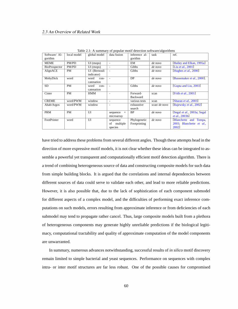
2.3 An Overview of Related Work
Table 2.1: A summary of popular motif detection software/algorithmsSoftware/ Al-gorithm
local model global model data fusion inference al-gorithm
task ref.
MEME PM/PD UI (mops) - EM de novo [Bailey and Elkan, 1995a]BioProspector PM/PD UI (mops) - Gibbs de novo [Liu et al., 2001]AlignACE PM UI (Bernouli
indicator)- Gibbs de novo [Hugheset al., 2000]
MobyDick word word con-catenation
- DP de novo [Bussemakeret al., 2000].
SD PM word con-catenation
- Gibbs de novo [Gupta and Liu, 2003]
Cister PM HMM - Forward-Backward
scan [Frith et al., 2001]
CREME word/PWM window - various tests scan [Sharanet al., 2003]Ahab/Argos word/PWM window - exhaustive
searchscan/de novo [Rajewskyet al., 2002]
PRM PM UI sequence +microarray
BP de novo [Segalet al., 2003a; Segalet al., 2003b]
FootPrinter word UI sequenceof multiplespecies
PhylogeneticFootprinting
de novo [Blanchette and Tompa,2003; Blanchette et al.,2002]
have tried to address these problems from several different angles. Though these attempts head in the
direction of more expressive motif models, it is not clear whether these ideas can be integrated to as-
semble a powerful yet transparent and computationally efficient motif detection algorithm. There is
a trend of combining heterogeneous source of data and constructing composite models for such data
from simple building blocks. It is argued that the correlations and internal dependencies between
different sources of data could serve to validate each other, and lead to more reliable predictions.
However, it is also possible that, due to the lack of sophistication of each component submodel
for different aspects of a complex model, and the difficulties of performing exact inference com-
putations on such models, errors resulting from approximate inference or from deficiencies of each
submodel may tend to propagate rather cancel. Thus, large composite models built from a plethora
of heterogeneous components may generate highly unreliable predictions if the biological legiti-
macy, computational tractability and quality of approximate computation of the model components
are unwarranted.
In summary, numerous advances notwithstanding, successful results ofin silico motif discovery
remain limited to simple bacterial and yeast sequences. Performance on sequences with complex
intra- or inter motif structures are far less robust. One of the possible causes for compromised
60

2.4 MotifPrototyper: Modeling Canonical Meta-Sequence Features Shared in a Motif Family
generalizability and scalability of many extant algorithms is believed to be their incorrect inde-
pendence assumptions about motif sites and motif occurrences, which leads to inability to cap-
ture possible intra-motif spatial dependencies corresponding to the signature physical structure for
unique recognition and stable molecular interaction, and inter-motif dependencies that elicit syn-
ergy or simply avoid overlap. As mentioned in the introduction, there have been some recent at-
tempts at addressing these issues at various levels[Hertz and Stormo, 1999; Heldenet al., 2000;
Frith et al., 2001; GuhaThakurta and Stormo, 2001; Rajewskyet al., 2002; Barashet al., 2003;
Nazina and Papatsenko, 2004]. In the following, we will develop an expressive modular motif
model that builds on these previous lines of research.
2.4 MotifPrototyper: Modeling Canonical Meta-Sequence FeaturesShared in a Motif Family
For the gene regulatory system to work properly, a TF must display much higher binding affinities to
its own recognition sites than to non-site DNA. This correspondence suggests possible regularities
in the DNA motif structure that match the structural signatures in the DNA-binding domains of their
corresponding TFs. Can these regularities hidden in the true DNA motif patterns be exploited to
improve sensitivity and specificity during motif discovery? As Michael Eisen has pointed out (pri-
vate communications), there should be great potential for improving motif recognition by modeling
and exploiting such structural regularities.
As reviewed in the previous sections, all extant local models of DNA motifs are essentially
motif-specific and are intended to generalize only to different instances of the same motif. An im-
portant issue that remains little addressed is how to build models that can generalize over different
motifs that are somewhat related (for instance, belonging to a family of regulatory sites that are
targets of TFs bearing the same class of binding domains) even though they do not share appar-
ent commonality in consensus sequences. This issue is important in computational motif analysis
because,
• often, we want to roughly predict the biological property of anin silico identified motif pattern
61

2.4 MotifPrototyper: Modeling Canonical Meta-Sequence Features Shared in a Motif Family
(e.g., to what kind of TFs it is likely to bind) to reduce the search space of experimental
verification;
• we may need to introduce some generic but biologically meaningful bias duringde novomotif
detection so that we can distinguish a biologically plausible binding site (i.e., specifically
recognizable by some TF) from a trivial recurring pattern (e.g., micro-satellites);
• we may also want to restrict attention to a particular class of proteins in performing tasks
such as: “find a regulatory site that potentially binds to type X TF”, or “find co-occurring
regulatory sites that can be recognized by type X and type Y TFs, respectively.”
These tasks are important in inferring gene regulatory networks from genomic sequences, possibly
in conjunction with relevant expression information.
In this section, we address the problem of modeling generic features ofstructurally but not
textuallyrelated DNA motifs, that is, motifs whose consensus sequences are entirely different, but
nevertheless share “meta-sequence features” reflecting similarities in the DNA binding domains of
their associated protein recognizers. We present MotifPrototyper, a profile hidden Markov Dirichlet-
multinomial (HMDM) model which can capture regularities ofnt-distribution prototypesandsite-
conservation couplingstypical to each particular family of motifs that corresponds to TFs with
similar types of structural signatures in their DNA binding domains. Central to this framework is
the idea of formulating a profile motif model as a family-specific structured Bayesian prior model
for the PWMs of motifs belonging to the family being modeled, thereby relating these motif patterns
at themeta-sequence level. In the following, after a brief discussion of the biological motivation
underlying our model, we will first develop the theoretical framework of the HMDM model, and
then show how to learn family-specific profile HMDMs, or MotifPrototypers, from biologically
identified motifs categorized in standard biological databases; how the model can be used as a
classifier for aligned multiple instances of motifs; and most importantly, how a mixture model
built on top of multiple profile models can facilitate Bayesian estimation of the PWM of a novel
motif. The Bayesian estimation approach connects biologically identified motifs in the database
62

2.4 MotifPrototyper: Modeling Canonical Meta-Sequence Features Shared in a Motif Family
to previously unknown motifs in a statistically consistent way (which is not possible under the
single-motif-based representations described previously) and turnsde novomotif detection, a task
conventionally cast as anunsupervisedlearning problem, into asemi-unsupervisedlearning problem
that makes substantial use of existing biological knowledge.
2.4.1 Categorization of Motifs Based on Biological Classification of DNA BindingProteins
TF categorization from TRANSFAC r6.0Superclass class # of training matrices # of test
alignments1.1 : Leucine zipper factors (bZIP) 341.2 : Helix-loop-helix factors (bHLH) 131.3 : Helix-loop-helix/leucine zipper factors 221.4 : NF-1 61.5 : RF-X 1
1:Basic domains
1.6 : bHSH 6
82 48
2.1 : Cys4 zinc finger or nuclear receptor type 142.2 : diverse Cys4 zinc fingers 132.3 : Cys2His2 zinc domain 212.4 : Cys5 cycteine-zinc cluster 3
2:Zinc-coordinatingDNA-bindingdomains
2.5 : Zinc fingers of alternating composition 1
52 36
3.1 : Homeo domain 413.2 : Paired box 63.3 : Fork head / winged helix 43.4 : Heat shock factors 73.5 : Tryptophan clusters 17
3:Helix-turn-helix
3.6 : TEA domain 1
76 64
4.1 : RHR (Rel homology region) 154.2 : STAT 134.3 : p53 24.4 : MADs box 94.5 : β-Barrelα-helix TFs 14.6 : TATA-biding proteins 34.7 : HMG 54.8 : Heteromeric CCAAT factors 94.9 : Grainyhead 24.10: Cold-shock domain factors 0
4:beta-scaffold fac-tors
4.11: Runt 1
60 13
0: Other TFs . . . . . . 1
Table 2.2: The TRANSFAC categorization of transcription factors (for the training set, the counts are made on TFs thathave more than 10 biologically identified binding sites; for the test set, TFs with at least 6 sites are counted.)
Unlike proteins or genes, which usually have a one-to-one correspondence to monomer se-
quences and hence are directly comparable based on sequence similarity, a DNA motif is a collective
object referring to a set of similar short DNA substrings that can be recognized by a specific protein
transcription factor. Different motifs are characterized by differences in consensus, stochasticity
63

2.4 MotifPrototyper: Modeling Canonical Meta-Sequence Features Shared in a Motif Family
and number of occurrences. Since each motif usually corresponds to a profile of gap-less, multiple-
aligned instances rather than a single sequence as for genes and proteins, comparisons based on
sequence similarity for different motif patterns are not as straightforward as for genes or proteins.
From a biological point of view, perhaps the most informative way of categorizing DNA motifs
is according to the regularities of the DNA-binding domains of their corresponding transcription
factors. Advances in structural biology have provided an extensive categorization of the biophysical
structures of DNA-binding proteins. The most recent update of the TRANSFAC database[Wingen-
deret al., 2000] lists 4219 entries, many of which are homologous proteins from different species
but are nevertheless indicative of the vast number of transcription factors now known that regulate
gene expression. Table2.2 shows a fraction (the top two levels in the cluster hierarchy) of the
TRANSFAC categorization of TFs. This categorization provides a good indication of the types of
binding mechanisms involved in motif-TF recognition. For concreteness, the following is a brief
summary of the structural regularities of four of the major classes of DNA-binding proteins, para-
phrasing[Stryer, 1995]. Due to the correspondence between a TF and a DNA motif, the TF catego-
rization strongly suggests possible features in the structure of motif sequences that are intrinsic to a
family of motifs corresponding to a specific class of TFs.
Theleucine zippersignature (Figure2.4a) under the superclass of basic-domain is an important
feature of many eukaryotic regulatory proteins. The hallmark of leucine zipper proteins is the
presence of leucine at every 7th position in a stretch of 35 residues. This regularity suggests the
presence of a zipper-likeα-helical coiled coil bringing together a pair of DNA-binding modules to
bind two adjacent DNA sequences. Leucine zippers can couple identical or nonidentical chains,
suggesting a homodimeric or heterodimeric signature in the recognition site. A variation of this
structural theme often seen in prokaryotic transcription factors is thehelix-loop-helixsignature. In
this case, the basic DNA-binding helices are connected into a dimer by a short loop.
The zinc finger domain (Figure2.4b) is also common in eukaryotic TFs and regulates gene
expression by binding to extended DNA sequences. A zinc finger grips a specific region of DNA,
binds to the major groove of DNA and wraps part of the way around the double helix. Each finger
64

2.4 MotifPrototyper: Modeling Canonical Meta-Sequence Features Shared in a Motif Family
(a) leucine zipper (b) zinc fingers
(c) helix−turn−helix (d) beta scaffold
Figure 2.4: DNA binding domains in TFs.
makes contact with a short stretch of the DNA, and residues from the amino-terminal part of the
α-helix form hydrogen bonds with the exposed bases in the major groove. Zinc-finger DNA binding
proteins are highly versatile and can have various numbers of zinc fingers in the binding domain.
Arrays of zinc fingers are well suited for combinatorial recognition of DNA sequences.
The helix-turn-helix domain (Figure2.4c) contains twoα-helices separated by 34A - the pitch
of a DNA double helix. Molecular modeling studies showed that these two helices would fit into
two successive major grooves. This domain, common in bacterial DNA-binding proteins, such
as the bacteriophageλ Cro protein, also occurs in the eukaryotic homeobox proteins controlling
development in insects and vertebrates.
The beta-scaffold factors (Figure2.4d) are somewhat unusual in that they bind to the minor
groove of DNA. The binding domain is globular rather than elongated, suggesting extensive contact
between the DNA sequence and the protein binding domain.
65

2.4 MotifPrototyper: Modeling Canonical Meta-Sequence Features Shared in a Motif Family
0
1
2
bits
5′
1TAG
2
G
3GA
4TG
5CAT
6T 7 8CGA
9
C
10
GCAT
11 12
AC
13
TCG
3′
0
1
2
bits
5′
1TA
CG
2
C
3
C
4CGA
5
T
CG
6CG
7
T
CG
8TC
GA
9AT
10
T
G
AC
11
G
12
G
ACT
13
G
14
T
A
GC
15
GC
16
GCT
17
TGC
3′
gal4−permute
pho4−permute
0
1
2
bits
5′
1
C
2
G
3CG
4CGA
5TA
CG
6
T
A
GC
7TC
GA
8TGC
9AT
10
T
CG
11
GCT
12
T
G
AC
13
T
CG
14
G
ACT
15
GC
16
C
17
G3′
0
1
2
bits
5′
1CAT
2 3GCAT
4 5CGA
6AC
7GA
8
C
9
G
10
T
11
TG
12
TCG
13
TAG
3′
gal4
pho4
Figure 2.5: Conservation-coupling of a zinc-finger motifgal4 and a helix-loop-helix motifpho4. Since typicalconservation-couplings are often reflected in the “contour shape” (e.g.,U- or bell-shape) of the motif logo (a graph-ical display of thespatial pattern of information content over all sites), we can understand this property as a “shapebias”.
These class-specific protein-binding mechanisms suggest the existence of features that are char-
acteristic of different families of DNA motifs, and shared by different motifs in the same family.
It is evident that the positions within the motifs are not necessarily uniformly conserved, nor are
the conserved positions randomly distributed. Since only a subset of the positions inside the motif
are directly involved in protein binding, the degree of conservation of positions inside the motif is
likely to be spatially dependent, and such dependencies may be typical for each motif family cor-
responding to a TF class due to structural complementarity between motifs and the corresponding
TFs. It is also possible that due to different degrees of variability-tolerance for different TF classes,
each family of motifs may require a different selection of prototypes for the distributions of possible
nucleotides at the positions within the motifs. Note that such regularities are less likely to be pre-
served in a non-functional recurring pattern, thus they also provide important clues to distinguishing
genuine from false motif patterns duringde novomotif finding. Figure2.5provides two examples
for the so-calledconservation-couplingproperty of the position dependencies in functional motifs.
On the left-hand side are two genuine motifs from two different families. On the right are artifi-
cial patterns resulting from a column permutation of the original motifs. Although the two patterns
will receive the same likelihood score under conventional PWM representations, clearly the pat-
terns on the left are biologically more plausible because of the complementarity of their patterns of
conserved positions to the structures of their binding proteins. Again, it is important to remember
that the conservation-coupling property and nt-distribution prototypes are only associated with the
generic biophysical properties of a motif family, butnot with any specific consensus sequence of a
single motif; thus, they are calledmeta-sequence features.
66

2.4 MotifPrototyper: Modeling Canonical Meta-Sequence Features Shared in a Motif Family
2.4.2 HMDM: a Bayesian Profile Model for Motif Families
The goal is to build a statistical model to capture the generic properties of a motif family so that it
can generalize to novel motifs belonging to the same family. In the following we develop such a
model using a hierarchical Bayesian approach.
The column of nucleotides at each position in a motif can be modeled by aposition specific
multinomial distribution(PSMD). A multinomial distribution overK symbols can be viewed a
point in a regular(K − 1)-dimensional simplex; the probabilities of the symbols are the distances
from the point to the faces of the simplex (an example of a 2-dimensional simplex is shown in
Figure2.6a). A Dirichlet distribution is a particular type of distribution over the simplex, hence a
distribution over the multinomial distributions. Each specific Dirichlet is characterized by a vector
of K parameters. It can impose a bias toward a particular type of PSMD in terms of how strongly
it is conserved, and to what nucleotide it is conserved. For example, in Figure2.6a, the center of
probability mass is near the center of the simplex, meaning that the multinomial distributions that
define a near uniform probability for all possible nucleotides will have a higher prior probability.
But for a Dirichlet density whose center of mass is close to a corner associated with a particular
nucleotide, say, “A” (Figure2.6b), the multinomial distributions with high frequencies for “A” have
high prior probabilities. Therefore, we can regard a Dirichlet distribution as a “prototype” for the
PSMDs of motifs.
(a) (b)
Figure 2.6: Dirichlet densities over a three-nucleotide simplex.
We propose a generative model that generates a multi-alignmentA containingM instances of a
motif of lengthL, in the following way (as illustrated in Figure2.7). 1) Sample a sequence of states
67

2.4 MotifPrototyper: Modeling Canonical Meta-Sequence Features Shared in a Motif Family
s = (s1, . . . , sL) from a first-order Markov chain with initial distributionυ and transition matrix
Υ. The states in this sequence can be viewed as prototype indicators for the columns (positions)
of the motif. Associated with each state, is a corresponding Dirichlet distribution specified by the
value of the state. For example, ifsl = i, then columnl is associated with a Dirichlet distribution
αi = [αi,1, . . . , αi,4]t. 2) For eachl ∈ 1, . . . , L, sample a multinomial distributionθl according
to p(θ|αsl), the probability defined by the Dirichlet componentαsl
. 3) Generate all the nucleotides
in columnl iid according to the multinomial distribution parametrized byθl.
Is s
θ θ θ
1 2 L
1 2 L
...
...
s
Am,1
MMM
Am,2 Am,L
profile HMDP
α
υ,Υ
Figure 2.7: The graphical model representation of a MotifPrototyper. Empty circles represent random variables associatedwith a single motif and the boxes are plates representingiid replicates (i.e.,M observed instances of the motif). Blackarrows denote dependencies between the variables. Parameters of the MotifPrototyper are represented by the center-dotted circles, and the round-cornered box over theα parameter denotesI sets of Dirichlet parameters. The round-cornered dashed box denotes plate of parameters of a single HMDM model, and hence represent a possible mixture ofHMDMs.
Thus, the complete likelihood of a motif alignmentAM×L characterized by a nucleotide-count
matrixh is:
p(A, s, θ|α, υ,Υ) = p(A|θ)p(θ|s, α)p(s|υ,Υ). (2.17)
where (using the update properties of the Dirichlet distribution and lettingsil = 1 if sl is at statei
and 0 otherwise)
p(h|x, θ)p(θ|s, α) =L∏
l=1
I∏i=1
Dir(αi + hl)sil , (2.18)
p(s|υ,Υ) =I∏
i=1
[υi]si1
L−1∏l=1
I∏i,j=1
[Υi,j ]sils
jl+1 . (2.19)
68

2.4 MotifPrototyper: Modeling Canonical Meta-Sequence Features Shared in a Motif Family
Technically, such a model, which is named aMotifPrototyper, is ahidden Markov Dirichlet-
multinomial model. It defines a structured prior for the PWM of a motif.
With the availability of a categorization for motifs, each family of motifs can be associated with
a family-specific profile HMDM model that imposes PSMD prototypes and positional-dependencies
unique to this family.
What do we gain from a MotifPrototyper? First, a MotifPrototyper introduces prior information
about the joint distribution of the nt-distribution in different positions of a motif of the corresponding
family, and gives high probabilities to those commonly found distributions possibly compatible
with the degree of variability-tolerance intrinsic to the class of TFs corresponding to the motif
family. Under a MotifPrototyper,a posteriori, each PSMD in a motif follows a family-specific
mixture of multiple Dirichlet distributions, which blends the different prototypes that might dictate
the nt-distribution at that position. Furthermore, a MotifPrototyper stochastically imposes family-
specific spatial dependencies for different columns within a motif. As Figure2.7 makes clear, a
MotifPrototyper isnot a simple HMM for sequence data. In an HMM model the transitions would
be between the emission models (i.e., multinomials) themselves, and the output at each step would
be a single monomer in the sequence. In MotifPrototyper, the transitions are between different prior
components for the emission models, and the direct output of this HMM is the parameter vector of
a generative model, which will be sampled multiple times at each position to generateiid instances.
This approach is especially useful when we have prior knowledge about motif properties, such as
conservation-couplingor other positional dependencies. In contract to the IC profile used in the
constrained PM model, due to the stochastic nature of a probabilistic model, MotifPrototyper will
in general not be rigidly confined to any particular motif shape (unless we explicitly forbid certain
transitions in the transition matrixΥ of the hidden Markov chain). These properties relieve our
motif model from the restricted, often brittle constraints needed in other models, such as exactly
what shape to look for, the widths of the conserved and unserved patches in a motif, the length of
the whole motif1, etc., and as a result provide desirable flexibility and robustness under practical
1In an HMDM model, the length of the motif pattern to be modeled does not have to be rigorously defined but only
69

2.4 MotifPrototyper: Modeling Canonical Meta-Sequence Features Shared in a Motif Family
motif detection environment.
Secondly, rather than using a maximum likelihood (ML) approach to estimate the PWM, which
considers only the relative frequency of nucleotides but is indifferent to the actual number of in-
stances observed, MotifPrototyper facilitates a Bayesian estimation of the PWM under a family-
specific prior, thus taking into consideration the actual number of observations available for PWM
estimation along with the biological prior. It is possible with only a few instances to obtain a robust
estimation of the nucleotide frequency at each position of a motif.
Note that a MotifPrototyper defines a family-specific structured prior for the PWMs without
committing to any specific consensus motif sequence.
2.4.2.1 Training a MotifPrototyper
Given biologically identified instances of motifs of a particular family, we can compile a multiple-
alignment for each motif and write down the joint likelihood of the training data under a single
profile model (i.e., a MotifPrototyper) by marginalizing out the PWMs (i.e.,θ’s) and the hidden
Markov states (i.e.,s) of each motif in Eq. (2.17). This likelihood is a function of the model
parameters. Thus we can compute the empirical Bayes estimation of the model parameters,Θl :=
α, υ,Υ, by maximizing the likelihood over each parameter using a EM algorithm with a quasi-
Newton procedure for the parameter update step[Sjolanderet al., 1996] (see AppendixA.2 for
details). The result is a set of parameters intrinsic to the training data.
Note that this training process also involves a model selection issue of how many Dirichlet
components should be used. As in any statistical model, a balance must be struck between the
complexity of the model and the data available to estimate the parameters of the model. Empirically,
we found that 8 components appears to be a robust choice and also provides good interpretability.
needs a rough specification (e.g., a length, say,L =20 bp, that is unlikely to be exceeded by most of the plausible motifs).Because under the HMDM model, both conserved and heterogeneous sites are allowed in a candidate motif pattern; amotif whose length is smaller thanL can still be picked up by the model with a over-specified length with high probabilityby allowing heterogeneous sites padded at the ends of the true motif pattern to make up the total length.
70

2.4 MotifPrototyper: Modeling Canonical Meta-Sequence Features Shared in a Motif Family
2.4.3 Mixture of MotifPrototypers
Now we have built a model that captures the meta-sequence features of structurally but not textually
related motifs. The model is a Bayesian profile model that is defined on each motif family rather than
each individual motif; thus we call it a MotifPrototyper. To estimate the PWM of a novel motif, since
we do not know which family-specific MotifPrototyper is corresponds best to the novel pattern, we
can assume that the motifs are generated from a weighted combination of several MotifPrototypers.
Statistically, this defines a mixture of MotifPrototypers as the prior distribution of the PWM of a
motif,
p(θ|α, υ,Υk, k = 1, . . . ,K) =K∑
k=1
wkp(θ|α, υ,Υk), (2.20)
wherewk is the mixing weight of each family-specific MotifPrototyper.
Under this setting, one can perform several important probabilistic computations regarding
motif detection, such as classifying motifs in terms of their preferred binding protein family by
identifying the most likely MotifPrototyper for a given motif alignment; computing the Bayesian
estimations of the motif parameters; and biasing thede novomotif detection to solutions that are
structurally more consistent with biologically genuine motifs. In other words, we effectively turn
the originally unsupervisedde novomotif detection into a semi-unsupervised learning problem that
integrates the observed sequences with prior knowledge about motif structures.
2.4.3.1 Classifying motifs
Identifying that a motif belongs to a family, and relating it to other members of the family, often
allows inference about its functions. Given multiple profile models each corresponding to a distinct
motif family, we can compute the conditional likelihood of a set of aligned instances of an unlabeled
motif under each profile model by integrating out the hidden variables (i.e.,θ ands) in each result-
ing complete likelihood function. The posterior probability of each possible assignment of class
membership to the motif under test is proportional to the magnitude of the conditional likelihood
multiplied by the prior probabilities of the respective motif families (which can be computed from
the empirical frequency of each motif family). LettingZ denote the family membership indicator,
71

2.4 MotifPrototyper: Modeling Canonical Meta-Sequence Features Shared in a Motif Family
the posterior probability ofZ = k is proportional to the magnitude of the conditional likelihood
under thekth MotifPrototyper multiplied by the prior probability ofZ = k:
p(Z = k|A) ∝ p(Z = k)p(A|α, υ,Υk)
Thus, we can estimate the family membership by amaximum a posteriori(MAP) scheme. It is
noteworthy that, here, we are classifying a set of aligned instances of a motif as a whole, rather than
a single sequence substring as in a standard classification task, such as predicting the function or
structure of a protein based on its amino acid sequence[Karchinet al., 2002; Moriyama and Kim,
2003].
2.4.3.2 Bayesian estimation of PWMs
Given a set of aligned instances of a motif, if we know the family membership of this motif, we can
directly compute the posterior distribution of its PWM, using the family-specific MotifPrototyper
as a prior according to Bayes rule. The Bayesian estimate of a PWM is defined as the expectation
of the PWM w.r.t. this posterior.
If the family membership is not knowna priori (i.e., we do not pre-specify what family of motif
to look for, but allow the motif to come from any family), then we can simply assume that the PWM
admits a mixture of profile models. The posterior distribution of a PWM under a mixture prior is
only slightly more complex:
p(θ|A, α, υ,ΥKk=1) =
∑k
p(θ|A, α, υ,Υk, Z = k)p(Z = k|A, α, υ,ΥKk=1)
∝∑
k
p(θ|A, α, υ,Υk)p(A|α, υ,Υk)p(Z = k), (2.21)
whereZ denotes the family membership indicator. A useful variant of this mixture model is to
replace the mixture with the maximal-likelihood component:
p(θ|A, α, υ,ΥKk=1) ≡ p(θ|A, α, υ,Υk∗), wherek∗ = arg max
kp(A|α, υ,Υk).(2.22)
It is straightforward to generalize the current formulation of the MotifPrototyper model to
family-specific prior distributions over more sophisticated motif representations, such as trees or
72

2.4 MotifPrototyper: Modeling Canonical Meta-Sequence Features Shared in a Motif Family
mixture of trees, by slightly reparameterizing the MotifPrototyper model. The training procedure
and the usage for classification andde novomotif detection require little modification.
2.4.3.3 Semi-unsupervisedde novomotif detection
In de novomotif detection where locations of motif instances are not known, the motif matrixA
is an unobserved random variable. One can iterate between predicting motif locations based on the
current Bayesian estimate of the motif PWM, and updating the Bayesian estimate based on newly
predicted motif instances. We will elaborate on this point in§2.5, where we describe aLOGOS
model that uses MotifPrototyper as the local model and an expressive hidden Markov model to
be developed in the next section, CisModuler, as the global model, forde novomotif detection in
higher eukaryotic genomic sequences. But as a “prove-of-concept” demonstration of the influence
of MotifPrototyper on the performance ofde novomotif detection, in this section, we only use a
simple oops model as the global model. It can be proved that the iterative procedure we described
is guaranteed to converge to a locally optimal solution (cf. Chapter 4). But unlike the standard EM
algorithm for estimating a PWM, since we can compute the Bayesian estimate based on a trained
profile motif prior, we essentially turnde novomotif detection from an originally unsupervised
learning problem into a semi-unsupervised learning problem that can make use of biological training
data without committing to any particular consensus motif pattern.
2.4.4 Experiments
Under theLOGOS framework, the MotifPrototyper and mixture of MotifPrototypers are both struc-
tured Bayesian upgrades of the standard PM local models for motifs. These models can be learned
from categorized training motifs to define family-specific priors for the PWMs, and when coupled
with a global model, can be used to introduce useful bias duringde novomotif detection.
In this sub-section, we present results of learning MotifPrototyper models from categorized
families of motifs, and demonstrate applications of the learned MotifPrototypers with three exper-
iments, each addressing a typical issue of interest inin silico motif analysis. (1) Given instances
of a (computationally) identified motif, assign the motif to a motif family that corresponds to a
73

2.4 MotifPrototyper: Modeling Canonical Meta-Sequence Features Shared in a Motif Family
particular class of transcription factors. (2) Provide a Bayesian estimate of a PWM which may
be more informative than a maximum likelihood estimate. (3) Improvede novomotif detection by
casting the problem as asemi-supervised learningtask that makes use of biological prior knowledge
incorporated in the family-specific MotifPrototypers.
2.4.4.1 Parameter estimation
The TRANSFAC database (version r6.0) contains 336 nucleotide-count matrices of aligned motif
sequences. These matrices summarize a significant portion of the biologically identified transcrip-
tion regulatory motifs reported in the literature, and are well categorized and curated. (Although
the original aligned sequences corresponding to the count matrices are not provided.) We used 271
of the matrices as training data, each derived from at least 10 recognition sites of a TF in one of
the 4 well-represented superclasses (Table2.2), to compute the empirical Bayes estimates of the
parameters of 4 profile Bayesian models of motif families.
2 4 6 8
2
4
6
8
2
4
6
8
A C G T0
5
10
A C G T0
5
10
A C G T0
5
10
A C G T0
5
10
A C G T0
5
10
A C G T0
5
10
A C G T0
5
10
A C G T0
5
10
A C G T0
5
10
A C G T0
5
10
A C G T0
5
10
A C G T0
5
10
A C G T0
5
10
A C G T0
5
10
A C G T0
5
10
A C G T0
5
10
2
4
6
82 4 6 8
1
2
3
4
5
6
7
8
A C G T0
5
10
A C G T0
5
10
A C G T0
5
10
A C G T0
5
10
A C G T0
5
10
A C G T0
5
10
A C G T0
5
10
A C G T0
5
10
2
4
6
82 4 6 8
1
2
3
4
5
6
7
8
00.5
1
(color scale: )
2
4
6
82 4 6 8
1
2
3
4
5
6
7
8
A C G T0
5
10
15
20
A C G T0
5
10
15
20
A C G T0
5
10
15
20
A C G T0
5
10
15
20
A C G T0
5
10
A C G T0
5
10
A C G T0
5
10
A C G T0
5
10
Basic domain Zinc−fingers
Helix−turn−helix Beta−scaffold
Υα υ υ Υα
Figure 2.8: Parameters of 4 profile models learned from training motifs. Each of the 8 panels underα represents the4-dimensional parameter vector of a Dirichlet component (the height of the bar represents the magnitude of the corre-sponding element in the vector); vectorυ and matrixΥ are represented by color images, of which each element ofυ orΥ specifies the color of a rectilinear patch in the image.
We performed 50 random restarts for the quasi-Newton algorithm for parameter estimation and
picked the solutions corresponding to the highest log likelihood achieved at convergence. Figure2.8
illustrates the parameters of the 4 resulting profile models pictorially. Here we do not intend to fully
74

2.4 MotifPrototyper: Modeling Canonical Meta-Sequence Features Shared in a Motif Family
interpret these numerical representations of each profile model in terms of their biological impli-
cations. But based on a rough inspection, it is not difficult to read off some interesting high-level
biological characteristics. For example, for thebasic-domainprofile model, the transition probabil-
ities between the 4 conserved nt-distribution prototypes2 (the first four mixture components of the
Dirichlet mixture) appear to be rather high (evident from the bright diagonal block at the upper left
corner of theΥ matrix), as are the self-transition probabilities of all of the 4 non-conserved Dirichlet
components (evident from the bright diagonal stripe at the lower right corner of theΥ matrix). The
transition probabilities between the conserved and non-conserved Dirichlet components are rela-
tively low (dark off-diagonal areas inΥ). Furthermore, it appears that the initial probability is high
for the 6th Dirichlet component, a fairly non-conserved one. This suggests a general meta-sequence
feature, namely that motifs of the basic-domain family are likely to begin with a consecutive run of
mostly non-conserved positions, followed by a consecutive stretch of mostly conserved positions,
and possibly followed by another consecutive run of mostly non-conserved positions, reminiscent of
the bell-shaped signature in Figure2.5. Although it is possible to find many other similar high-level
characteristics, some of which may even reveal previously unnoticed biological features (e.g., char-
acteristic PSMD prototypes of motif families), here we refrain from such elaborations, but simply
maintain that MotifPrototyper is a formal mathematical abstraction of the meta-sequence properties
intrinsic to a motif profile represented by the training examples.
To evaluate the training quality of the profile models, we define thetraining error as the per-
centage of misclassification of the superclass-identities of the training motif matrices using profile
models learned from the full training set. As Table2.3 shows, our training errors range from 10-
28%, with the beta-scaffold MotifPrototyper having the best fit. Given that “motif family” is rather
loosely defined based on TF superclasses, and that each superclass still has very diverse and ambigu-
ous internal structures, these training errors indicate that family-specific regularities can be captured
2Note that the parameter vector of a Dirichlet component can be regarded as a vector of pseudo-counts of thenucleotides. Thus a Dirichlet parameter vector with a dominant element implies a conserved nt-distribution proto-type, whereas a Dirichlet parameter vector without a dominant elements implies a heterogeneous, or non-conservednt-distribution prototype.
75

2.4 MotifPrototyper: Modeling Canonical Meta-Sequence Features Shared in a Motif Family
reasonably well by MotifPrototyper.
Table 2.3: Learning MotifPrototyperBasic domains Zinc-fingers Helix-turn-helix beta-scaffold
training error 0.168 0.173 0.276 0.100
2.4.4.2 Motif classification
To examine the generalizability of MotifPrototyper to newly encountered motif patterns, we per-
formed a 10-fold cross-validation (CV) test for motif classification, in which the profile models are
learned from 90% of the training motif matrices, and their classification performance is evaluated
on the remaining 10% of the motif matrices. We do so 10 times so that each motif pattern corre-
sponding to a particular TF will be classified exactly once as a test case. The performances over
each family of motifs are summarized in Table2.4. Classification error rates for both the entire
dataset and the reduced dataset that contains only the major motif subclasses (i.e., those with at
least 10 different motifs) under each superclass are presented. Not surprisingly, performance on the
dataset with only major subclasses is significantly better, suggesting that the minor classes in each
superclass are possibly more ambiguous and less typical with respect to the overall characteristics
of the superclass. In fact, some minor classes are unanimously assigned to a different superclass
by our classifier, for example, all 6 members of class 1.6 (bHSH) and all 7 members of class 3.4
(heat shock factors) are assigned to superclass 4 (beta-scaffold), whereas all 5 members of class 4.7
(HMG) are assigned to superclass 3 (helix-turn-helix). Whether such inconsistencies reflect a defi-
ciency of our classifier or possible true biological ambiguity of these motif patterns is an interesting
problem to be investigated further.
Table 2.4: Motif classification using MotifPrototyperBasic domains Zinc-fingers Helix-turn-helix Beta-scaffold
CV error (whole set) 0.256 0.423 0.443 0.403CV error (major classes) 0.217 0.373 0.379 0.178
To our knowledge, there has been no algorithm that classifies aligned sets of motif instances as
76

2.4 MotifPrototyper: Modeling Canonical Meta-Sequence Features Shared in a Motif Family
collective objects based on meta-sequence features shared within motif families. The closest coun-
terpart in sequence analysis is the profile HMM (pHMM) model for protein classification[Kroghet
al., 1994], but pHMM is based on the assumption that proteins of the same family share sequence-
level similarities, and the objects classified are single sequences. Thus, no direct comparison can be
made between pHMM and MotifPrototyper. Nevertheless, note that although pHMM is based on
much more stringent features at the sequence level and aimed at the relatively simpler task of eval-
uating single sequences, the typical accuracy of pHMM is around 20-50% for short polypeptides
(i.e.,< 100 aa)[Karchinet al., 2002; Moriyama and Kim, 2003], comparable to the performance of
motif classification using MotifPrototyper. Thus we believe that MotifPrototyper exhibits a reason-
able performance given that the labeling of motif family membership is more ambiguous than that
of single protein sequences, the meta-sequence features we use are far less stringent than sequence
similarities, and motif patterns are much shorter than polypeptides.
2.4.4.3 PWM estimation and motif scoring
A major application of MotifPrototyper is to serve as an informative prior for Bayesian estimation
of the PWM from a set of aligned instances of a novel motif. Since in a realisticde novomotif
detection scenario, one has to evaluate many substrings corresponding to either a true motif, or ran-
dom patterns in the background, it is expected that the Bayesian estimate of a PWM resulting from
MotifPrototyper is more reliable than the maximum likelihood estimate in discriminating between
true motifs and background sequences. We demonstrate this ability by comparing the likelihood of
a true motif substring with the likelihoods of background substrings, all scored under the estimated
PWM of the motif. To get an objective evaluation for this comparison, the following experiments
were performed: 1) for a set of aligned instances of a motif, compute the Bayesian estimate of the
PWM from 66% of the instances, and then use it to score (i.e., compute the likelihood of) the re-
maining 34% of the instances in terms of their joint log likelihood; 2) use the same PWM to score
M sets of background strings, each having the same length and number of instances as the motif
instances being scored in step 1; 3) compute the mean log-likelihood-odds between the motif and
77

2.4 MotifPrototyper: Modeling Canonical Meta-Sequence Features Shared in a Motif Family
the background substrings (overM sets of randomly sampled background substrings). For each
motif, we repeat this procedure 3 times so that each motif substring will be scored exactly once.
The performance on each motif is summarized by the average log-likelihood-odds per motif in-
stance. (Larger odds means that the background substrings are less likely to be mistakenly accepted
as motif instances, and thence, the false positive rate is smaller).
Since the original aligned motif sequences corresponding to the count matrices used for Mo-
tifPrototyper training are not provided in TRANSFAC and are hard to retrieve from the original
literature, we compiled an independent collection of aligned motif instances for 161 TFs in TRANS-
FAC, each of which has at least 6 binding sites whose sequence information is available (Table2.2).
Background substrings from a uniform and random model were simulated3.
0 20 40 60 80 100 120 140 160−100
0
100
200
300
400
500
600
700
800
900
log
−lik
elih
oo
d o
dd
s /
inst
an
ce
motif types0 10 20 30 40 50 60 70 80
−100
−50
0
50
100
150
200
250
300
350
400
log−
likelih
ood o
dds
/ in
stance
motif types0 10 20 30 40 50
−100
0
100
200
300
400
500
600
700
800
900
log
−lik
elih
oo
d o
dd
s /
inst
an
ce
motif types
all motifs motifs with > 10 instances motifs with <10 instances
Figure 2.9: Evaluation of PWM estimation by 4 different schemes. Cyan:symmetric-Dirichlet smoothing; green: ML;red: mixture of profile models; black: maximal-likelihood profile model out of the mixture. Motifs are listed along thex-axis, ordered by the log-likelihood-odds of their PWM based on the “true” (according to their original family label)profile prior model.
The results of the evaluation are highlighted in Figure2.9. We compared 4 PWM estimation
schemes: maximum likelihood estimation (i.e., plain relative frequencies); Bayesian smoothing
using a single symmetric Dirichlet prior; Bayesian estimation using a mixture of profile models;
and Bayesian estimation using the maximal-likelihood profile model from the mixture. Depicted
as the bars in Figure2.9 for reference are the results for Bayesian estimation using a single profile
model corresponding to the original family label of each motif, an unrealistic scenario inde novo
3This corresponds to examining the log-likelihood-odds under a motif model w.r.t. a uniform and random null hy-pothesis. Sampling of background substrings from a genuine genomic sequence as the null hypothesis was also doneat a small scale (for some motifs) and yields largely the same results. But since the motifs we studied are from diversegenomic sources, a comprehensive evaluation in this manner is tedious and hence was omitted.
78

2.4 MotifPrototyper: Modeling Canonical Meta-Sequence Features Shared in a Motif Family
motif detection.
As evident from Figure2.9and2.10, the discriminative power of the Bayesian estimate of the
PWM, measured by the log-likelihood-odds (of motif vs. background substrings), is indeed better
than that of the maximum likelihood estimate for most of the motifs we tested. In particular, in
cases where only a small number of instances are available for estimation, the mixture of profile
models still leads to a good estimate that generalizes well to new instances and results in high
log-likelihood-odds, whereas the ML estimation does not generalize as well (Fig.2.9).
0 50 100 150 200 250 300 350
0
50
100
150
200
250
300
350
Bay
esia
n E
st. o
f PW
M
ML Est. of PWM
Figure 2.10: A comparison of Bayesian and ML estimates of the PWM. Each point represents a motif being tested, thex-coordinate (resp.y-coordinate) represents the log-likelihood-odds due to the ML (resp. Bayesian) estimation.
These results give strong support to the claim that in many cases, a MotifPrototyper-based
approach can significantly improve the sensitivity and specificity for novel motifs, and provide a
robust estimation of their PWMs under few observations. These are very useful properties forde
novomotif detection in complex genomic sequences.
2.4.4.4 De novomotif discovery
Now we present a comparison of the profile Bayesian motif model – MotifPrototyper – with the
conventional PM model forde novomotif detection, using semi-realistic test data for which the
ground truth (i.e., full annotation of motif types and locations) is known for evaluating the prediction
results. Note that the experiments described here are a small excerpt from a large suite ofde novo
motif detection experiments under various scenarios. We will return to the bulk of these experiments
79

2.4 MotifPrototyper: Modeling Canonical Meta-Sequence Features Shared in a Motif Family
in §2.7, after the development of a more powerful global model.
We tested on 28 well-represented yeast motifs from thePromoter Database of Saccharomyces
cerevisiae(SCPD). Each motif has 5 to 32 recorded instances, all of which have been identi-
fied/verified via biological experiments and hence are considered “authentic”. For each motif, a
test dataset is created by planting each of the “authentic” instances of that motif at a random posi-
tion in a 500bp simulated background sequence (i.e., one motif per sequence). To further increase
the difficulty of the motif detection task, a “decoy” signal, which is an artificial pattern obtained by
randomly permuting the positions in the motif, was inserted into the study sequence4. Since each
sequence has only one true motif occurrence, prediction was made by finding the position with the
maximal log-likelihood ratio (for the substring that begins with that position) under the estimated
motif PWM (obtained at the convergence point of a procedure that iterates between computing the
posterior distribution of motif locations based on current estimate of the PWM, and computing the
Bayesian estimate of the PWM based on the current posterior distribution of motif locations), and
under the background nt-distribution (assumed to be the nt-frequencies estimated from the entire
sequence). This scenario frees us from modeling the global distribution of motif occurrences, as
needed for more complex sequences (cf. the LOGOS model), and therefore demonstrates the in-
fluence of different models for motif patterns onde novodetection. We evaluate the performance
based onhit-rate, the ratio of correctly identified motif instances (within± 3bp offset with respect
to the locations of the authentic instances) to the total number of instances to be identified. To obtain
robust estimation, for each motif 40 experiments were performed, each with a different test dataset
(i.e., with different background sequences, motif and decoy locations, and decoy patterns).
Specificity of a single MotifPrototyper. Before presenting the full-scale test of the mixture of
MotifPrototypers trained on four categories of motifs from the TRANSFAC database on the yeast
motifs from the SCPD database, here we first examine whether the motif properties captured in
a MotifPrototyper effectively bias the posterior prediction of motif presence toward the desired
4By permutation we mean that the same permuted order is applied to all the instances of a motif so that the multinomialdistribution of each position is not changed but their order is changed.
80

2.4 MotifPrototyper: Modeling Canonical Meta-Sequence Features Shared in a Motif Family
pattern represented in the training set. For this purpose we trained a MotifPrototyper from the 28
yeast motifs in the SCPD database described above, and examined the resulting MotifPrototyper for
its ability to detect motifs present in this training set in the presence of a “decoy”. Figure2.11shows
the Boxplot (which shows the median, lower quartile, upper quartile, outliers, etc.) of the hit (i.e.,
finding the genuine motif) and mishit (i.e., finding the decoy) rate of MotifPrototyper onabf1and
gal4. Note the dramatic contrast of the specificity of the MotifPrototyper to true motifs compared
to that of the PM model.
It is noteworthy that the MotifPrototyper model actually does not contain any explicit infor-
mation about the consensus sequences of the training motifs; it merely captures the dependencies
between general heterogeneous and homogeneous motif sites whose nucleotide distributions are not
fixed, but instead are drawn from specified priors over the space of nucleotide distributions. Thus,
the high specificity of MotifPrototyper to a genuine motif pattern under the interference of a false
motif pattern suggests its remarkable ability to implicitly capture sensible “motif shapes”.
1 20
0.2
0.4
0.6
0.8
1
gal4 (hit)
1 2
0
0.2
0.4
0.6
0.8
1
gal4 (mis−hit)
1 2
0
0.2
0.4
0.6
0.8
1
abf1 (hit)
1 2
0
0.2
0.4
0.6
0.8
1
abf1 (mis−hit)
Figure 2.11: Boxplots of hit and mishit rate of MotifPrototyper (1) and PM (2) on two motifs used during MotifPrototypertraining.
Generalizability of a single MotifPrototyper. How well does a MotifPrototyper generalize to
motifs not present in the training set? Here we use the MotifPrototyper learned from 20 of the 28
SCPD motifs to detect motifs from an independent test set containing the rest of the 8 SCPD motifs.
In the first motif finding task, we use synthetic sequences each having only one true motif instance
at a random position. Figure2.12summarizes the results over 40 experiments. As shown in the
figure, the MotifPrototyper significantly outperforms the PM model for motifsabf1, gal4 andcrp,
and achieves comparable performance for motifsgcn4andmig1. It does poorly for motifsmat-a2
andmcb. Note that these two motifs are quite short and somewhat uniformly “conserved,” which is
81

2.4 MotifPrototyper: Modeling Canonical Meta-Sequence Features Shared in a Motif Family
in fact “atypical” in the training set. The smallish sizes of the motifs also diminish the utility of the
Markov model in MotifPrototyper.
1 20
0.2
0.4
0.6
0.8
abf1
1 2
0
0.2
0.4
0.6
0.8
1
gal4
1 2
0
0.2
0.4
0.6
0.8
gcn4
1 2
0
0.2
0.4
0.6
0.8
gcr1
1 20
0.2
0.4
0.6
0.8
1
mat−a2
1 2
0
0.2
0.4
0.6
0.8
1
mcb
1 20
0.2
0.4
0.6
0.8
1
mig1
1 2
0
0.2
0.4
0.6
0.8
crp
Figure 2.12: Boxplots of hit rate of MotifPrototyper (1) and PM (2) on sequences each embedded with one motif instancefrom the test dataset.
In the foregoing motif detection task, the PM model shows decent performance, especially for
those more-or-less uniformly conserved motifs such asgcn1, mat andmcb. But it already shows
signs of failure for motifs with more complex shapes (e.g.gal4). The second task is more challeng-
ing and biologically more realistic, where we have both the true motifs and the permuted “decoys.”
Figure 2.13 shows the boxplot of the hit-rate as well as the mishit-rate for motif detection over
40 experiments. As expected, under the interference of the decoys, the PM model apparently gets
confused and often decides to pick the permuted false motifs. Only two of the eight motifs are cor-
rectly detected by the PM model with high hit-rate. In contrast, the MotifPrototyper model exhibits
remarkable robustness under this more difficult situation, and maintains a high hit-rate in six of the
eight motifs. But for two of the motifs (again,mat-a2andmcb), MotifPrototyper biases toward the
permuted version, which suggests that indeed the originalmat-a2andmcbpatterns are not captured
by MotifPrototyper, consistent with the result from the first task.
De novomotif detection using a mixture of MotifPrototypers. Now we conclude this section
with an evaluation of a mixture of MotifPrototypers trained from the TRANSFAC database. We
test this model on all the 28 motifs from the SCPD database. As shown in Figure2.14, the mixture
of MotifPrototypers significantly outperforms the PM model (i.e. with> 20% margin) on 11 of
the 28 motifs, and is comparable to the PM model (within±10% difference) for the remaining
82

2.4 MotifPrototyper: Modeling Canonical Meta-Sequence Features Shared in a Motif Family
1 20
0.2
0.4
0.6
0.8
abf1
1 2
0
0.2
0.4
0.6
0.8
1
gal4
1 2
0
0.2
0.4
0.6
0.8
gcn4
1 2
0
0.2
0.4
0.6
0.8
gcr1
1 20
0.2
0.4
0.6
0.8
1
mat−a2
1 2
0
0.2
0.4
0.6
0.8
mcb
1 2
0
0.2
0.4
0.6
0.8
1
mig1
1 2
0
0.2
0.4
0.6
0.8crp
1 20
0.2
0.4
0.6
0.8
abf1
1 2
0
0.2
0.4
0.6
0.8
gal4
1 2
0
0.2
0.4
0.6
gcn4
1 2
0
0.2
0.4
0.6
0.8
gcr1
1 20
0.2
0.4
0.6
0.8
1
mat−a2
1 2
0
0.2
0.4
0.6
0.8
mcb
1 2
0
0.2
0.4
0.6
0.8
1
mig1
1 2
0
0.2
0.4
0.6
0.8crp
Figure 2.13: Boxplots of hit (left panel) and mishit (right panel) rates of MotifPrototyper (1) and PM (2) on sequenceseach containing one motif instance from the test dataset together with a permuted decoy.
17 motifs. Overall, the mixture of MotifPrototypers correctly identifies 50% or more of the motif
instances for 16 of the 28 motifs, whereas the PM model achieves 50% hit-rate for only 8 of the
28 motifs. Note that the mixture of MotifPrototypers is fully autonomous and requires no user
specification of which particular profile motif model to use. If we are willing to introduce a manual
post-processing step, in which we use each of the 4 profile motif models described before separately
for de novomotif finding, and generate 4 sets of motif predictions instead of one (as for the mixture
of MotifPrototypers) for visual inspection, it is possible to obtain even better predictions (diamond
symbols in Figure2.14).
−0.2
0
0.2
0.4
0.6
0.8
1
med
ian
hit−
rate
motif types
gcn4
gcr1
mcb
bas1
−pho
2H
SE
,HTS
Fua
shph
o2ga
taha
p1ua
sphr
gal4
rep−
car1
tbp
mig
1re
b1ta
ta−t
bpra
p1cc
bf−s
wi6
abf1
CS
RE
mcm
1ro
x1st
e12
mat
−a2
pho4
pdr1
scb
urs1
h
Figure 2.14: Median hit-rates ofde novodetection of 28 yeast motifs using MotifPrototyper (square), PM (circle), andthe best outcome out of 4 single-profile-based predictions using MotifPrototyper (diamond). Motifs are listed along thex-axis, ordered by the hit-rates of MotifPrototyper for each motif.
The ability to provide multiple candidate solutions, each corresponding to a specific TF cate-
gory, manifests a key advantage of the profile motif model. It allows a user to capture different
types of prior knowledge about motif structures and bias motif prediction toward a particular meta-
sequence structure in a well-controlled way. A human observer given a visual presentation of the
most likely motifs suggested by different profile motif models could easily pick out the best one
83

2.4 MotifPrototyper: Modeling Canonical Meta-Sequence Features Shared in a Motif Family
from these candidates, whereas the PM model can yield only a singlemost likelyanswer.
2.4.5 Summary and Discussion
We have presented MotifPrototyper, a novel profile Bayesian motif model that captures generic
meta-sequence featuresshared by motifs corresponding to common transcription factor superclasses.
It is a probabilistic graphical model that captures the positional dependencies and nucleotide dis-
tribution prototypes typical to each motif family, and defines a prior distribution of the position
weight matrices of motifs for each family. We demonstrated how MotifPrototyper can be trained
from biologically identified motif examples, and its applications for motif classification, Bayesian
estimation of PWMs, andde novomotif detection.
To the best of our knowledge, all extant motif models are intended to be motif-specific, empha-
sizing the ability to characterize sequence-level features unique to a particular motif pattern. Thus
when one defines such a model for a novel motif not biologically characterized before, one needs to
solve a completely unsupervised learning problem to identify the possible instances and fit the motif
parameters simultaneously. Under this unsupervised framework, there is little explicit connection
between the novel motif to be estimated from the unannotated sequences and the rich collection
of biologically identified motifs recorded in various databases. It is reasonable to expect that the
fruitful biological investigations of gene regulatory mechanisms and the resulting large number of
known motifs could contribute more information to the unraveling of novel motifs. MotifProto-
typer represents an initial foray into the development of a new framework that turnsde novomotif
detection into a semi-unsupervised learning problem. It provides more control during the search
for novel motif patterns by making use of prior knowledge implied in the known motifs, helps to
improve sensitivity to biologically plausible motifs, and potentially reduces spurious solutions often
occurred in a purely unsupervised setting.
It may be possible to build a stronger motif classifier using discriminative approaches such as
neural networks or support vector machines, and we are currently pursuing this direction. But since
the goal of this chapter is not merely to build a classifier, but to develop a model that can easily
84
2.5 CisModuler: Modeling the Syntactic Rules of Motif Organization
be integrated into a more general architecture forde novomotif detection, a generative framework,
especially via a Bayesian prior model, provides the desired generalizability and flexibility for such
tasks. As discussed in§2.2.4, a graphical model formalism of the motif detection problem allows
a modular combination of heterogeneous submodels each addressing a particular component of the
overall problem. The design of MotifPrototyper aligns with this principle, and serves as an advanced
“local” submodel under theLOGOS framework.
2.5 CisModuler: Modeling the Syntactic Rules of Motif Organization
As discussed in previous sections, the transcription regulatory sequences in higher eukaryotic genomes
often consist of multiple CRMs. Each CRM contains locally enriched occurrences of binding sites
for a certain array of regulatory proteins, capable of integrating, amplifying or attenuating multi-
ple regulatory signals via combinatorial interaction with these proteins. The architecture of CRM
organization is reminiscent of the grammatical rules underlying a natural language, and provides
the potential for implementing sophisticated regulatory circuits directing temporally/spatially co-
ordinated expression of genes during development and differentiation. It also presents a particular
challenge to computational motif and CRM identification in higher eukaryotes. In this section, we
present CisModuler, a Bayesian hidden Markov model that attempts to capture the stochastic syn-
tactic rules of CRM organization and integrates over (and thus draws influence from) all possible
values of the Markov transition probabilities weighted by their corresponding prior probabilities
that reflect general knowledge of the CRM structure. Under the CisModuler model, all candidate
sites are evaluated based on a posterior probability measure that takes into consideration their sim-
ilarity to known binding sites, their contrasts against local genomic context, and their first-order
dependencies on upstream sequence elements. We compare this approach to the standard window-
based likelihood scoring approach described previously, and demonstrate superior results on large
scale analysis ofDrosophilaearly developmental enhancers. This model provides a useful and ar-
guably superior alternative for CRM/motif detection given motif PWMs, and can be also used as a
submodel (i.e., the global model) forde novomotif/CRM detection in higher eukaryotic genomes.
85

2.5 CisModuler: Modeling the Syntactic Rules of Motif Organization
2.5.1 TheCisModulerHidden Markov Model
Hidden Markov models have been widely used in computational biology to capture simple sequence
structures (e.g., segmentations) inherent in bio-polymer sequences. Despite their limited expressive
power compared to more complex models such as stochastic context free grammars (SCFGs)[Lari
and Young, 1990] or hierarchical hidden Markov models (hHMMs)[Fine et al., 1998], they have
enjoyed remarkable success in problems such as gene-finding in DNAs[Burge and Karlin, 1997]
and domain modeling in proteins[Krogh et al., 1994], and in many cases appear to strike the right
balance between simplicity and expressiveness.
We propose to use an HMM to model the global distribution of motif instances in genomic
sequences, by encoding a set of stochastic syntactic rules presumably underlying the CRM organi-
zation and motif dependencies using a discrete first-order Markov process. We call this specialized
HMM a CisModuler. The CisModuler HMM defines a probability distribution over possible func-
tional states of each single position in a DNA sequence. The space of allowed functional states
is constructed in a way that captures detailed architectural features of genomic sequences bearing
CRMs.
More precisely, letX = (X1, . . . , XT ) be a chain of “hidden” state variables associated with
an “observed” DNA sequencey = (y1, . . . , yT ), specifying which functional state (e.g., a back-
ground, thel-th position of motifk, etc.) is responsible for generating the observed nucleotide at
each position. By definition,xt ∈ S, where the state spaceS includes all possible functional states
of a position in a CRM-bearing DNA sequence. Specifically,S = M ∪ M′ ∪ Bp ∪ Bd ∪ bg, bc,
whereM = 1(1) . . . L(1)1 , 1(2) . . . L(2)
2 , . . . , 1(k) . . . L(k)k is the set of all possible sites within a motif
on the forward DNA strand (i.e., states1(1) to L(1)1 correspond to the sites in motif type 1 on the
forward strand, and so on);M′ is the set of all possible sites within a motif if it is on the reverse
complementary DNA strand;Bp = b(1)p , . . . , b(k)p denotes the set ofproximal-bufferstates associ-
ated with each type of motif5; Bd = b(1)d , . . . , b(k)d denotes the set ofdistal-bufferstates associated
5Here, proximal-buffer refers to the background sites immediately next to the proximal-end of the motif. For consis-tency, orientations are defined with respect to the initial position of the input sequence. That is, the 1st position of theinput sequence corresponds to the proximal end, and the last position corresponds to the distal end.
86

2.5 CisModuler: Modeling the Syntactic Rules of Motif Organization
with each type of motif;bc represents the intra-cluster (local) background state; andbg represents
the inter-cluster (global) background state. Permissible transitions between these states are illus-
trated in Figure2.15. The distribution ofX follows a first-order Markov process according to this
transition scheme, with state-transition probabilities parameterized as shown in the state-transition
diagram. Note that we have not included functional states related to gene annotation and basal pro-
moters, but such extensions are straightforward if co-identification of CRMs and genes is desired.
(1) (1) (1)...1 2 L
(1’)... 1L(1’) 2 (1’)1
1
1
1
1
1
βk,1
β1,k
βk,k
1
1
1
1
(k) (k) (k)...1 2 L
(k’)...L(k’) 2 (k’) 1
k
k
β1,1
c,cβ
g,gβ
βg,1
βg,k
β1,g
βk,g
β c,1 β c,kβk,c
β1,c
...α/2
α/2
α/2
α/2
1
1
1
1
global bg
cluster bg
Motif 1
Motif k
buffer
buffer buffer
buffer
(a)
(b)
Figure 2.15: The CisModuler HMM. (a) The state-transition diagram. Labeled circular and diamond nodes represent thefunctional states in DNA sequences; arrows between nodes represent permissible state-transitions; numbers and param-eter symbols accompanied the arrows (with the parameter subscripts denoting the source and target of the transitions)denote the corresponding transition probabilities. (b) A typical segmentation of a piece of DNA sequence induced byCisModuler. Background sites are colored as in the state-transition diagram; the blue, magenta, yellow and red segmentsrepresent motifs of 4 different kinds; segments with parallel stripes denote motifs in reverse-complementary orientation.
The motivation for this Markov model is that generally one expects to see occasional motif clus-
ters in a large ocean of global background sequences (represented by statebg). Each motif instance
87

2.5 CisModuler: Modeling the Syntactic Rules of Motif Organization
in a cluster is like an island in a sea of intra-cluster background sequences (bc’s), with surrounding
coastal water of motif-specific buffer sequences (i.e.,b(i)p ’s andb(i)d ’s for motif i) (Fig. 2.15). We
refer to a motif instance together with its surrounding buffers as amotif envelope. The CisModuler
model assumes that the distance between clusters is geometrically distributed with mean1/(1−βg,g),
and the span of the intra-cluster sea is also geometrically distributed with mean1/(1− βc,c). How-
ever, the distances between motifs admit a much richer distribution, because the widths of the motif
envelopes are modeled on a motif-specific basis, and the transitions between envelopes can occur ei-
ther by sailing through the intra-cluster sea or by bypassing it. These modeling choices are intended
not only to reflect uncertainty about the CRM structure, but also to offer substantial flexibility to
accommodate potential richness of CRM structures. As shown in Figure2.15a and2.15b, one can
begin with a global background state, then either loop over this state, or with some probabilityβg,i,
move into the proximal-buffer state of a motifi; with equal probabilityαi,m/2, a proximal-buffer
stateb(i)p reaches the start states1(i) (resp. L(i′)i ) of motif i on the forward (resp. reverse) strand,
deterministically passes through all internal sites of motifi, and transitions to the distal-buffer state
b(i)d , thereby stochastically generating a non-empty motif envelope6; eachb(i)d has some probability
βi,j/2 of transitioning to the proximal-buffer state of another motifj (or of the same motif when
j = i) to concatenate another motif envelope, or with probabilityβi,c to pad with some intra-cluster
background before adding more envelopes; all distal-buffer states also have probabilityβi,g of re-
turning to the global background state, terminating a CRM stretch. It is not difficult to see that a
path in such a state space according to this HMM grammar bears a structure similar to a genomic
sequence containing motif modules (Figure2.15b). Note that the HMM model does not impose
rigid constraints on the number of motif instances or modules; the actual number of instances is
determined by the posterior distribution of the sequence of functional states,p(x|y).
The use of an HMM to model the CRM distribution has been previously described by Frithet
al. in the Cister program[Frith et al., 2001]. But the CisModuler model we present here uses a
6Note that the distinction between the proximal and distal buffers avoids generating empty envelopes (because other-wise, a single buffer state would not be able to remember whether a motif has been generated beyondk positions prior tothe current position under akth order Markov model.)
88

2.5 CisModuler: Modeling the Syntactic Rules of Motif Organization
much more sophisticated design of the functional state space that allows couplings between motifs
within the CRMs to be captured, and models inter-motif distances with more flexible distributions
(rather than a simple geometric distribution). Furthermore, as will be detailed in the following
sections, we provide a Bayesian treatment for the state transition probabilities, which in previous
models are regarded as fixed parameters and rely on empirical default values or user specification.
We also combine the newly designed HMM with a more expressivekth-order Markov model for
the background, which turns out to contributes to significantly improving the specificity for CRM
detection.
2.5.2 Bayesian HMM
One caveat of the standard HMM approach for CRM modeling is the difficulty of fitting the model
parameters, such as the state-transition probabilities, due to the scarcity of fully annotated CRM-
bearing genomic sequences. In principle, one can learn the maximal likelihood estimates of the
model parameters in an unsupervised fashion, using the Baum-Welch algorithm, directly from the
unannotated sequences while analyzing them. But in practice, such a completely likelihood-driven
approach tends to result in spurious results, such as over-estimation of the motif and CRM frequen-
cies and poor stringency of the learned models of potential motif patterns. Previous methods tried to
overcome this by reducing as much as possible the number of parameters needed, and setting them
according to some best guesses of the motif/CRM frequencies or CRM sizes[Frith et al., 2001]. But
as a result, such remedies compromise the expressive power of the already simple HMM, and risk
misrepresenting the actual CRM structures. In the following, we propose a Bayesian approach that
introduces the desired “soft constraints” and smoothing effect for an HMM of rich parameteriza-
tion, using only a small number ofhyper-parameters. Essentially, this approach defines a posterior
probability distribution over all possible value-assignments for the HMM parameters, given the ob-
served unannotated sequences and empirical prior distributions of the parameters that reflect general
knowledge of CRM structures. The resulting model allows probabilistic queries (i.e., estimating the
probability of a functional state) to be answered based on the aforementioned posterior distribution
89

2.5 CisModuler: Modeling the Syntactic Rules of Motif Organization
rather than on fixed given values of the HMM parameters.
We assume that the self-transition probability of the global background stateβg,g, and the to-
tal probability mass of transitioning into a motif-buffer state∑
k∈Bpβg,k (note thatβg,g = 1 −∑
k∈Bpβg,k), admit a beta distribution,Beta(ξg,1, ξg,2), where a small value was chosen forξg,2
ξg,1+ξg,2,
corresponding to a prior expectation of a low CRM frequency. Similarly, a beta priorBeta(ξc,1, ξc,2)
is defined for the self- and total motif-buffer-going transition probabilities[βc,c,∑
k∈Bpβc,k] asso-
ciated with the intra-cluster background state; and another beta priorBeta(ξp,1, ξp,2) for the self-
and motif-going transition probabilities[αi,i, αi,m] associated with the proximal-buffer state of
a motif. Finally, it is assumed that, for the distal-buffer state, the self-transition probability, the
total mass of transition probabilities into a proximal-buffer state, the probability of transitioning
into the intra-cluster background, and the probability of transitioning into the global background,
[βi,i,∑
k∈Bpβi,k, βi,c, βi,g], admit a 4-dimensional gamma distribution,Gamma(ξd,1, ξd,2, ξd,3, ξd,4).
Note that due to conjugacy between the prior distributions described above and the corre-
sponding transition probabilities they model, the hyper-parameters of the above prior distribu-
tions can be understood aspseudo-countsof the corresponding transitioning events, which can
be roughly specified according to empirical guesses of the motif and CRM frequencies. But un-
like the standard HMM approach, in which the transition probabilities are fixed once specified,
the hyper-parameters only lead to a soft enforcement of the empirical syntactic rules of CRM
organization in terms of prior distributions, allowing controlled posterior updating of the HMM
transition probabilities during analysis of the unannotated sequences. For the CisModuler HMM,
we specify the hyperparameters (i.e., the pseudo-counts) using estimated frequencies of the cor-
responding state-transition events, multiplied by a “prior strength”N , which corresponds to an
imaginary “total number of events” from which the estimated frequencies are “derived”. That is,
for the beta priors, we let[ξ[·,1], ξ[·,2]] = [1 − ω[·], ω[·]] × N , where the “·” in the subscript denotes
either theg, c, or p state, andω[·] is the corresponding frequency. For the gamma prior, we let
[ξd,1, ξd,2, ξd,3, ξd,4] = [ωd,1, 1 −∑
j ωd,j, ωd,2, ωd,3] × N . Overall, 7 hyper-parameters need to
be specified (of course one can use different “strengths” for different prior, with a few additional
90

2.5 CisModuler: Modeling the Syntactic Rules of Motif Organization
parameters), a modest increase compared to the three needed in Cister[Frith et al., 2001].
2.5.3 Markov Background Models
Several previous studies have stressed the importance of using a richer background model for the
non-motif sequences[Liu et al., 2001; Huanget al., 2004]. In accordance with these results, Cis-
Moduler uses a globalkth-order Markov model for the emission probabilities of the global back-
ground state. For the emission probabilities of the intra-cluster background state and the motif-
buffer states, we used twolocal Markov models of orderm andm′, respectively. Since the models
are defined to belocal, the conditional probability of a nucleotide at a positiont is now estimated
from all (m + 1)- (resp. (m′ + 1)-) tuples from a window of2d (resp. 2d′) centered att. These
probabilities can also be computed off-line and stored for subsequent use. With a careful bookkeep-
ing scheme (i.e., using a “sliding window” to compute the local Markov model of each successive
position, each with a constant “update cost” based on the previous one, except for the initial win-
dow that needs a cost quadratic in the window size), this computation takes onlyO(T ) time. For
the emission probabilities of the motif states, we directly use the appropriate columns of nucleotide
frequencies in the PWM of the corresponding motif.
2.5.4 Posterior Decoding Algorithms for Motif Scan
2.5.4.1 The baseline algorithm
Given the initial state distribution and transition probability matrix of the HMM, the background
probabilities of each nucleotide, and the PWMs of the motifs to be searched for, the posterior prob-
ability distribution of the functional states at each position of the sequences,p(xt|y),∀t, can be
computed using the forward-backward algorithm. One can read off the functional annotation (or
segmentation) of the input sequences fromp(xt|y) according to amaximal a posteriori(MAP)
scheme, that is, the predicted functional state of positiont is:
x∗t = arg maxs∈S
p(Xt = s|y) (2.23)
Note that by using such a posterior decoding scheme (rather than the Viterbi algorithm), one
91

2.5 CisModuler: Modeling the Syntactic Rules of Motif Organization
integrates the contributions of all possible functional state paths for the input sequence (rather than
a single “most probable” path), into the posterior probability for each position. Therefore, although
the HMM architecture does not explicitly model overlapping motifs, the inference procedure does
take into account possible contributions of DNA binding sites interacting with competing TFs.
2.5.4.2 Bayesian inference and learning
Under the Bayesian framework described in§ 2.5.2, the parameters in the HMM are treated as con-
tinuous random variables (collectively referred to asΩ) with a prior distribution. Now to compute
the posterior probability of functional states needed in Eq. (2.23), one needs to marginalize out
these parameter variables:
p(xt|y) =∫p(xt|y,Ω)p(Ω|y)dΩ (2.24)
This computation is intractable in closed form. One approach to obtaining an approximate so-
lution is to use Markov chain Monte Carlo methods (e.g., a Gibbs sampling scheme). Here we use a
more efficient, deterministic approximation scheme based ongeneralized mean field(GMF) infer-
ence, also referred to asvariational Bayesian learning[Ghahramani and Beal, 2001] in the special
scenario that is applicable to our problem setting. We will discuss the theoretical and algorithmic
details of GMF inference at length in Chapter 4. Operationally, a posterior decoding algorithm un-
der the Bayesian HMM setting can be understood as replacing the single-round posterior decoding
with an iterative procedure consisting of the following two steps:
• Compute the expected counts for all state-transition events (i.e., sufficient statistics) using the
forward-background algorithm, usingcurrent values of the HMM parameters.
• Compute the Bayesian estimate (to be detailed shortly) of the HMM parameters based on
their prior distribution and the expected sufficient statistics from the last step.Update the
HMM parameters with these estimations.
This procedure is different from the standard EM algorithm which alternates between inference
about the hidden variables (the E step) and maximal likelihood estimation of the model parameters
92

2.5 CisModuler: Modeling the Syntactic Rules of Motif Organization
(the M step). In a GMF algorithm, the “M” step is a Bayesian estimation step, in which one com-
putes the posterior expectation of the HMM parameters, which will lead to an optimal lower bound
on the true likelihood of the data (which is intractable to compute exactly for a Bayesian HMM)
(see Chapter 4).
Now we outline the formulas for Bayesian estimation of the HMM parameters. Note that be-
cause the state-transition probability distributions (which are multinomial) and the prior distribu-
tions of the transition parameters (which are either beta or gamma) are conjugate-exponential[Beal
et al., 2001], we have to compute the Bayesian estimate of the logarithms of the transition parame-
ters (referred to as thenatural parameters) rather than of the parameters themselves. For example,
for the state-transition parameterβg,g, we have:
E[ln(βg,g)] =∫
βg,g
lnβg,gp(βg,g|ξg,1, ξg,2, E[ng,g])dβg,g
= Ψ(ξg,1 + E[ng,g])−Ψ(∑
j
ξg,j +∑k∈Bp
E[ng,k]), (2.25)
whereΨ(x) = ∂ log Γ(x)∂x = Γ(x)
Γ(x) is the digamma function;E[·] denotes the expectation with respect
to the posterior distribution of the argument; andng,g refers to the sufficient statistic of the parameter
βg,g (i.e., the counts of the transition eventg → g). The Bayesian estimate of the original parameter
is simplyβ∗g,g = exp(E[ln(βg,g)]). (In fact we keep using the natural parameterization in the actual
forward-background inference algorithm to avoid numerical underflow caused by a long product of
probability terms.) The individual “motif-buffer-going” probabilityβg,i can be estimated similarly.
The initial state probability of the the CisModuler HMM is not important for CRM prediction
as it only directly determines the functional state of the first position of the input sequences and its
influence diminishes quickly along the sequence. One can simply fix the initial state to be a global
background state with probability 1.
2.5.5 Experiments
Although the literature on transcription regulation mechanisms in higher eukaryotes is very rich,
there still exist great biological ambiguities in motif and CRM annotations in many metazoan
93

2.5 CisModuler: Modeling the Syntactic Rules of Motif Organization
genomes. To evaluate our model using relatively unambiguous criteria, we focus on 14 loci in the
Drosophilagenome that are well known to be involved in regulating the transcription ofDrosophila
early developmental genes (Table2.5). Papatsenkoet al. [2002] have carefully curated these loci
based on an extensive study of the literature. Their compilation delineates 19 best-known early
Drosophiladevelopmental enhancers from these loci, where reside binding sites for 3 maternal tran-
scription factors: Bicoid (Bcd), Caudal (Cad), Dorsal (DI), as well as the zygotic gap gene factors
Hunchback (Hb), Kruppel (Kr), Knirps (Kni), Tailless (Tll), and Gaint (Gt). To mimic the typical
motif/CRM search scenario in metazoan genomic analysis (i.e., using a single long sequence po-
tentially containing numerous motifs rather than multiple short promoter regions from co-regulated
genes of simple organisms such as yeast), for each locus we extract a 5000 to 20000 bp long ge-
nomic region surrounding the enhancers as input data. Note that it is possible that there may exist
additional unknown motifs/CRMs in these extended regions.
Table 2.5: Developmental regulatory loci inDrosophilagenome.locus (target gene) regulators length # of CRMs
Abdominal-A Hb, Kr, Gt, 10000 1Buttonhead Bcd, Hb 5000 1Engrailed Cad, Ftz 10000 1Even-skipped Hb, Kni, Bcd, Kr, Gt 20000 3Fushi-Tarazu Ftz, Ttk, Cad 10000 2Gooseberry Eve, Prd (HD) 10000 1Hairy Kr, Hb, Kni, Cad, Gt 10000 3Kruppel Bcd, Hb, Gt, Kni 10000 1Orthodentcile Bcd 5000 1Runt Kr, Gt, Hb, Kni 10000 1Spalt Bcd, Hb, Kr, Cad 10000 1Tailless Bcd, Cad 8227 1Ultrabithorax BRE Hb, Ftz, Tll 10000 1Ultrabithorax PBX Hb, Ftz, Tll 10000 1
As discussed above, the hyperparameters of the CisModuler model reflect prior beliefs about
the architectural features of the CRM structure, such as rough spans of the inter- or intra-module
background and distances between motif instances. We specify these hyperparameters as follows:
for the global background,ωg = 0.0002; for the intra-module background,ωc = 0.01; for the
proximal motif buffer,ωp = 0.1; for the distal buffer hyperparameters,ωd,1 = 0.1, ωd,2 = 0.4,
ωd,3 = 0.4; and for the strength of the hyperparameters,N = 500. The background probability
of the nucleotide at each position was computed locally using a 3rd-order Markov model from a
94

2.5 CisModuler: Modeling the Syntactic Rules of Motif Organization
sliding window of 600 bp centered at the corresponding position. Since we are scanning for known
motifs, the PWMs of the motifs to be found are taken from[Papatsenkoet al., 2002] and[Berman
et al., 2002].
2.5.5.1 MAP prediction of motifs/CRMs
The locations of individual motif instances and CRMs in a DNA sequence can be determined from
its associated state sequence that corresponds to the MAP states of all the DNA sites. Figure2.16a
shows the MAP states and the associated posterior probabilities of these states in a 5000 bp region
at theDrosophilabuttonhead locus. As shown in the graphical illustration below the MAP plot, this
region contains a CRM between positions 330 and 1504, and part of the coding sequence of the
buttonhead gene. Fine-grained annotations indicate that a core subregion at the proximal end of this
CRM (positions 447-660) harbors 5 Bcd motifs. Another 4 Bcd instances are clustered at the distal
end of this CRM (positions 1150-1354). Three additional motifs (2 Bcds and 1 Hb) are scattered in
the middle of this CRM, but they appear to be weaker matches to the motif consensus compared to
the ones in the core subregions[Papatsenkoet al., 2002]. Using MAP estimation under CisModuler,
7 of the 12 motifs, 3 in the proximal and 4 in distal subregions of the CRM, are identified and the
core regions of the buttonhead CRM are correctly identified. Overall, among the 335 motif instances
(of 11 different regulatory proteins) and 19 CRMs contained in the loci we analyzed, 80 motifs and
16 CRMs are correctly identified, out of a total prediction of 316 motifs and 51 CRMs.
Under the aforementioned parameterization of CisModuler, the sensitivity measure of our pre-
diction (i.e., correct predictions/total annotated motifs) is about25%. But it is worth pointing out
that this result is obtained at a very low noise-to-signal ratio (i.e., incorrect predictions/correct pre-
dictions) of less than 3. Most extant algorithms report a list of predictions ranked by the score and
provide no quantitative measure of prediction accuracy suitable for a comparison. A few extant
algorithms reported higher sensitivity, but at an extremely high N/S ratio. For example, the log-
odds-based MATCH program[Quandtet al., 1995] achieves a∼ 90% sensitivity with a N/S ratio of
95

2.5 CisModuler: Modeling the Syntactic Rules of Motif Organization
1379 and 784 for Ap-1 and NEAT sites, respectively; the more sophisticated comparative-genomics-
based rVista program[Lootset al., 2002] achieves a similar sensitivity with N/S ratios of about 69
and 38, respectively. Such a high N/S ratio can make experimental verification extremely hard or
even infeasible, significantly compromising the value of the predictions. Also worth mentioning is
that our CRM-prediction using CisModuler is even more reliable, with an84% sensitivity, and 2.18
N/S. Thus it is possible to first identify the CRMs using a coarser-grained model, and then zoom in
to find motifs within the CRMs using a finer-grained model.
Note that unlike many other scoring schemes for motif/CRM detection, such as the log odds
or likelihood score regularized by word frequencies, our MAP prediction does not require a cutoff
value for the scores, nor a window to measure the local concentration of motif instances, both of
which are difficult to set optimally. To show the potential advantage of the MAP approach, Fig2.16b
shows the log odds of all sites in the buttonhead locus. Simply from inspection, it is apparent that,
even though we compute the log odds based on a more discriminating Markovian background model
together with the motif PWMs, we end up with too many positive signals (i.e., peaks with log odds
> 0). Exponentiating the log odds of all sites and thus transforming them to likelihood ratios (the
lower small panel in the graph) can significantly improve the contrast, but compared to the MAP
plot and the sketch of the genomic structure of this region, pruning away noises via a good cutoff
value and scoring window is still a non-trivial task.
2.5.5.2 Motif/CRM prediction via thresholding posterior probability profile
The MAP prediction described in the previous section considers only a single (i.e. thea posteriori
most probable) functional state for each site in a DNA sequence, and to some degree underuses
the posterior probabilities of all possible functional states for each site. An alternative approach
is to use the full posterior probability distribution at each site as a score function, and analyze the
score profile of the whole sequence using strategies conventionally applied to log odds or likelihood
profiles, such as thresholding motif scores with a cutoff value (to qualify a motif instance) and
measuring local motif concentrations with a sliding window (to qualify a CRM).
96

2.5 CisModuler: Modeling the Syntactic Rules of Motif Organization
CRM CDS500 1000 1500 2000 2500 3000 3500 4000 4500 5000
0.1
0.2
0.3
0.4
0.5
0.6
0.7
0.8
0.9
1
1000 2000 3000 4000 50000
1
2
3
4
5
6
7
8
1000 2000 3000 4000 5000
−30
−20
−10
0
1000 2000 3000 4000 50000
500
1000
1500
2000
(a)
(b)
Figure 2.16: Motif- and CRM-scan using CisModuler. (a) MAP plot of the buttonhead locus under the CisModuler model.They axis denotes posterior probability, and thex axis represents sites in the sequence. The black curve correspondsto the global background state, the green curve corresponds to the intra-cluster background and buffer states, and othercolor curves correspond to various motif states (red:Hb, blue:Bcd, and dotted curves correspond to the state of a reverseoriented motif represented by the same color). For each site, only the posterior probability of the MAP state is plotted.(b) Log odds of each site under the motif PWM versus a 3rd-order local Markov background model. Only positive scores(i.e., higher motif prob. than background prob.) are shown in the large panel. Complete log odds profiles (includingthe negative scores that indicate the background) are shown in the upper small panel for reference. The likelihood ratioscores derived from the log odds are shown in the lower small panel. Between panels (a) and (b) is a graphical illustrationof the biological annotation of this region.
97

2.5 CisModuler: Modeling the Syntactic Rules of Motif Organization
0 0.2 0.4 0.60
5
10
15
20
25
30
Sensitivity
Noi
se/S
igna
l
Motif prediction (total map)
logoddsposteriorMAP
0 0.1 0.2 0.3 0.4 0.5 0.6 0.7 0.8 0.9 10
1
2
3
4
5
6
7
Sensitivity
Noi
se/S
igna
l
CRM prediction
logoddsposteriorMAP
(a) (b)Figure 2.17: Validation of the posterior score under CisModuler and the likelihood ratio score: trade-off between sensi-tivity and noise. (a) Motif detection. (b) CRM detection. The performance curves record sensitivity and N/S achieved ata wide range of score cutoff values.
Fig. 2.17a shows the trade-off between sensitivity and noise during motif detection, in terms of
the proportion of the known binding sites detected and the amount of concomitant noise generated.
Following[Huanget al., 2004], Fig.2.17a traces the balance of sensitivity versus N/S ratio achieved
at a wide range of score cutoffs. Two score profiles were analyzed, the posterior probability profile
computed using the CisModuler model for the 14Drosophila loci described before (red curve in
Fig. 2.17a), and a likelihood ratio profile for the same dataset computed using motif PWMs and
a 3rd-order local Markov model (black curve in Fig.2.17a). Overall, the CisModuler posterior
probability score outperforms the likelihood ratio score over the entire range of noise-to-signal
ratio. Although not directly comparable (since different datasets are used), the performance curve
is similar to that of[Huanget al., 2004] (or arguably better because of the longer input sequences
used and the presence of CRMs that complicate motif identifications.) It is interesting to note that
the MAP prediction seems to be trying to pick the best possible sensitivity in the low noise-to-signal
ratio region.
Fig. 2.17b shows the trade-off between sensitivity and N/S ratio for CRM (rather than motif)
detection. The following scheme were used to identify a CRM based on the score profile: under a
given cutoff value of motif score, if the motif density within a sliding window of lengthW is at least
c, the corresponding sequence stretch is regarded as covered by a CRM. A contiguous region swept
98

2.5 CisModuler: Modeling the Syntactic Rules of Motif Organization
by a sliding window that meets this criteria is regarded as a CRM. Following typical characteristics
of CRMs reported in the literature, we setW = 500 andc = 2%. The sensitivity of CRM detection
is defined to be the ratio of the number of correctly predicted CRMs to the total number of CRMs;
and the N/S ratio as the ratio of the total length of all predicted CRMs over the length of correctly
predicted CRMs. From Fig.2.17b, it appears that CisModuler slightly outperform the the likelihood
ratio scheme in the high N/S region, and is significantly better in the low N/S region. As mentioned
earlier, the MAP prediction finds a good trade-off between the sensitivity and N/S ratio.
From the experiments reported above, we are optimistic that CisModuler is superior in motif
and CRM detection in a complex genomic context. But to predict based on the full posterior prob-
ability profile, a cutoff value is needed to qualify the possible presence of motif instances, and a
window size will be used to infer CRMs based on within-window concentration. Usually, such val-
ues have to be carefully determined from a training dataset, or via a statistical significance criterion
as in[Huanget al., 2004]. As a reward, we can take advantage of both the motif dependencies and
syntactic architecture of motif distributions explicitly captured in the CisModuler, the flexibility of
the thresholding scheme, and the nice statistical guarantee provided by a significance test.
2.5.6 Summary and Discussion
In this section, we presented a model-based Bayesian approach for CRM and motif prediction,
which combines many of the desirable features provided by extant methods, and introduces several
important novel elements that overcome some of the shortcomings of extant methods. The exten-
sions and contributions includes: a more sophisticated HMM model that is intended to capture, to
a reasonable degree, the detailed syntactic structure of CRM andcis-regulatory regions containing
CRMs; Bayesian priors for various state-transition parameters of the HMM grammar, which in prin-
ciple alleviate user specification of model parameters7; and severalkth-order Markov models for
various types of background sequences.
We compared our approach to the standard likelihood-ratio (or log odds) scoring approach,
7Although sophisticated users could choose to decide the “strength” of the priors, or define their own priors.
99

2.6 LOGOS: for Semi-unsupervised de novoMotif Detection
and demonstrated superior results on large scaleDrosophilaearly developmental enhancer analysis.
CisModuler provides a useful and arguably superior alternative approach to detect CRM and motif
occurrences based on a given PWM, and can be also used as a subroutine inde novomotif/CRM
detection from higher eukaryotic genomes.
2.6 LOGOS: for Semi-unsupervisedde novoMotif Detection
Recall that under theLOGOS framework, the local, global and background submodels jointly de-
fine the likelihood of an observed DNA sequence that contains unspecified motifs. Each submodel
can be designed separately to address different aspects of the biological characteristics of a transcrip-
tional regulatory sequence, and combination of submodels each from a wide spectrum of possible
designs is possible. Therefore,LOGOS facilitates a flexible trade-off between expressiveness and
complexity for motif modeling.
Most extant models forde novomotif detection fall into the most basic submodel combination,
namely, a PM local model plus a UI global model (denoted byLOGOSpu in the sequel). Exam-
ples ofLOGOSpu include the basic models underlying the MEME[Bailey and Elkan, 1995a] and
AlignACE [Hugheset al., 2000] programs (although both programs have more sophisticated and
efficient implementation, e.g., more careful initiation schemes for over-represented words, which in
practice improve their performance over a basicLOGOSpu model).
Having both the MotifPrototyper model for local motif structure and the CisModuler model for
global motif organization (which also includes thekth-order Markov model for the background),
one can envisage a novel generative model for transcriptional regulatory sequences that is signifi-
cantly more expressive than any extant motif detection models. A graphical representation of such
a model, which is referred to asLOGOShh (standing for HMDM + HMM), is depicted in Fig-
ure2.18. (For simplicity, in the sequel we abbreviateLOGOShh with the unsubscripted “LOGOS”
when no confusion arises in the context, e.g., no comparison with other variations ofLOGOS is
being made.) Specifically, in such aLOGOS model, the functional annotations of a DNA sequence
that determine the motif locations and modular structures are determined by a CisModuler HMM
100

2.6 LOGOS: for Semi-unsupervised de novoMotif Detection
Figure 2.18: A modular construction of theLOGOShh model for motif-bearing sequences. For simplicity, only onepossible motif and one study sequence are included in this model.
model; but the emission probabilities of the motif states, or the PWMs of the motifs, are generated
from a MotifPrototyper model, whereby prior knowledge regarding both global motif organization
and local motif structure is incorporated forde novomotif detection, making it asemi-unsupervised
learningproblem. Note that the context-sensitive dependency induced by the latent motif indicator
x couples each sequence variable with all existing motif parameters. Thus the nucleotide identity of
any position in a sequence is determined by a complex dependency structure that captures intra and
inter motif dependencies reflecting both intrinsic structural properties and higher-level correlations
of the motifs (detailed in§4.7).
The expressiveness ofLOGOS comes at the cost of resulting in a very expensive computational
problem for probabilistic inference in this model. Specifically, the inference and learning problem
associated withLOGOS is that of computing the maximuma posterioriprediction of motif lo-
cations and the Bayesian estimate of motif PWMs. But unlike the situations we discussed when
dealing with only the MotifPrototyper or the CisModuler submodels ofLOGOS, which essentially
intend to solve only one of the two aforementioned queries assuming the solution to the other is
known, now one needs to solve the two queries jointly, and this turns out to be intractable due to the
101

2.6 LOGOS: for Semi-unsupervised de novoMotif Detection
exploded state space of the joint model.
Since no off-the-shelf exact algorithm works forLOGOS, some approximation schemes have
to be used. One option is to pursue a stochastic approximation using MCMC techniques such as
Gibbs sampling. In Chapter 5, we describe a Gibbs sampler algorithm for posterior inference on
LOGOS. But as demonstrated in a preliminary experiment on modest-sized input sequences (see
§4.7.2), the Gibbs sampler converges very slowly and appears impractical for supporting a realistic
motif detection program. In Chapter 4, we develop a deterministic approximation method called
generalized mean field inference. Essentially, a GMF algorithm alternates between solving one of
the two sub-problems mentioned before in the respective submodel ofLOGOS, conditioning on
the approximate solution of the other sub-problem, and then updating the approximate solutions
using the newly obtained solutions, which yields a better approximation. It can be shown that this
algorithm is guaranteed to converge to a locally optimal solution, and defines a lower bound on the
likelihood of the study sequences. A full description of the theory and algorithm of GMF inference
in general graphical models, and specifically the fixed-point equations for theLOGOS model, is
deferred to Chapter 4. In the following, we present an extensive validation of theLOGOS model
on fully annotated semi-realistic datasets and real genomic sequences from yeast, and a preliminary
test on a small set of unannotatedDrosophilagenomic sequences.
2.6.1 Experiments
2.6.1.1 Performance on semi-realistic sequence data
Recall that in§2.5, we validated the utility of the MotifPrototyper model forde novomotif de-
tection in conjunction with a trivial global model — oops, which assume one motif per sequence.
Now we consider a more realistic scenario, in which each study sequence contains multiple mo-
tifs. We compare three variants of theLOGOS model for this setting, ordered by decreasing model
expressiveness, HMDM+HMM (LOGOShh), PM+HMM (LOGOSph) and PM+UI (LOGOSpu).
Specifically, a slightly simplifiedLOGOShh is used for the task herein, where the global submodel
is a simpler HMM containing only a single global background state in addition to the motif states
102

2.6 LOGOS: for Semi-unsupervised de novoMotif Detection
(meaning that no CRM structure is modeled), rather than using the highly elaborated CisModuler
Bayesian HMM tailored for higher eukaryotic sequences.
Single motif, and multiple instances per sequence. Under a realistic motif detection condition,
the number of motif instances is unknown. Rather than trying all possible numbers of occurrences
suggested by the user or decided by the algorithm and reporting a heuristically determined plau-
sible number,LOGOS uses the global HMM model to describe a posterior distribution for motif
instances, which depends on both the prespecified indicator state transition probabilities and the ac-
tual sequencey to be analyzed. In this experiment, the transition probabilities are empirically set at a
default value to reflect our rough estimates of motif frequencies (i.e., 5%). But as more training data
of annotated regulatory sequences are collected, these parameters can be fit in a genome-specific
fashion.
Table 2.6: Performance ofLOGOS for single motif detection, with unknown number of instances per sequence.
motif LOGOShh LOGOSph LOGOSpu
name FP FN FP FN FP FN
abf1 0.3115 0.2116 0.6774 0.1957 0.7917 0.9123gal4 0.1569 0.1569 0.1895 0.1534 0.2917 0.7939gcn4 0.1820 0.2355 0.6142 0.2821 0 0.9594gcr1 0.1962 0.2134 0.3371 0.2038 0.3333 0.9437mat 0.0723 0.0337 0.3563 0 0.5000 0.9643mcb 0.3734 0.0910 0.3628 0.0792 0.3333 0.9431mig1 0.0774 0 0.0854 0 0.9764 0.1000crp 0.3768 0.3398 0.2727 0.5294 0 0.9487
Table2.6summarizes the performance of three variants ofLOGOS for single motif detection,
with an unknown number of instances per sequence. We present the median false positive (FP)
and false negative (FN) rates (in terms of finding each instance of the motifs within an offset of
3 bp) of motif detection experiments over 20 test datasets. Each test dataset consists of 20 se-
quences, each generated by planting (uniformly at random) 0–7 instances of a motif (real sites from
SCPD), together with its permuted “decoy,” in a 300–400 bp random background sequence. As
Table2.6 shows,LOGOSpu yields the weakest results, losing in all 8 motif detections (in terms
of (FP+FN)/2), suggesting that the conventional PM+UI model, which is used in MEME, and with
103

2.6 LOGOS: for Semi-unsupervised de novoMotif Detection
slight variation, in AlignACE and BioProspector, is not powerful enough to handle non-trivial de-
tection tasks as posed by our test set.LOGOSph improves significantly overLOGOSpu, even
yielding the best performance in one case (formcb), suggesting that the HMM global model we
introduced indeed strengthens the motif detector. Finally, as hoped,LOGOShh yields the strongest
results, performing best on 7 of the 8 motifs, convincingly showing that capturing the internal struc-
tures of motifs and making use of prior knowledge from known motifs, combined with the use of
the HMM global model, can yield substantially improved performance. Our results are reasonably
robust under different choices of the global HMM parameters.
Simultaneous detection of multiple motifs. Detecting multiple motifs simultaneously is ar-
guably a better strategy than detecting one at a time and then deleting or masking the detected
motifs, especially when motif concentrations are high, because the latter strategy mistakenly treats
the other motifs as background, causing potentially suboptimal estimation of both motif and back-
ground parameters. The global HMM model we propose readily handles simultaneous multiple
motif detection (say, findingK motifs at a time): we only need to encode all motif states into the
state spaceS of the motif indicatorX, and perform standard HMM inference. The locations of all
motifs can be directly read off from the state configuration ofx. Table2.7 summarizes the results
on 20 test sets each containing 20 sequences harboring motifsabf1, gal4 andmig1 (0–6 total in-
stances/seq). The upper panels show the predictive performance based on the optimal (in terms of
maximal log-likelihood ofy from 50 independent runs of the GMF algorithm) posterior expectation
of X. Note that with a MotifPrototyper local model,LOGOShh exhibits better performance. In the
lower panels, we show the best FP-FN results in the top three predictions (i.e., top 3 PWMs for each
of theK motifs we look for) made byLOGOS (note that ‘K-at-a-time’ prediction yields a total
of 3K possibly redundant motif patterns). This is close to the stochastic dictionary scenario where
the predicted motif is to be identified from the optimal dictionary of the patterns resulting from the
motif detection program[Gupta and Liu, 2003]. It is expected that a human observer could easily
pick out the biologically more plausible motifs when given a visual presentation of the most likely
104

2.6 LOGOS: for Semi-unsupervised de novoMotif Detection
motifs suggested by a motif finder.
Table 2.7: Simultaneous multiple motif detection (median FP-FN rate over 20 test sets containing three motifs.)
LOGOShh LOGOSph
FP FN FP FN
abf1 0.3591 0.3274 0.7778 0.7434MAP pre-diction gal4 0.1259 0.1714 0.3751 0.1491
mig1 0.3849 0.2243 0.3481 0
abf1 0.3841 0.2400 0.4721 0.3972best of top 3prediction gal4 0.0926 0.0986 0.2609 0.1255
mig1 0.1250 0.0333 0.2318 0
Detecting motifs of uncertain lengths. A useful property of the MotifPrototyper submodel is
that it actually does not need to know the exact lengths of the motifs to be detected, since the Mo-
tifPrototyper allows a motif to start (and end) with consecutive heterogeneous sites. Thus, a blurred
motif boundary is permissible, especially when the resulting window is large enough to cover at
least the entire length of the motif. As a result, we do not have to know the exact length of the
motif, but just need to roughly guess it conservatively, duringde novomotif detection. This is
another appealing feature ofLOGOS, which extends its flexibility. As shown in Table2.8, even
in simultaneous multiple motif detection, with improperly specified motif lengths,LOGOShh per-
forms nearly as well as when motif lengths are precisely specified, whereasLOGOSph is not as
good.
Table 2.8: Simultaneous detection of three motifs, with lengths improperly specified (18, 22, and 20 bp, respectively,instead of the actual 13, 17, and 11 bp).
LOGOShh LOGOSph
FP FN FP FN
abf1 0.7295 0.6667 0.8021 0.7680MAP pre-diction gal4 0.1167 0.2042 0.2357 0.1325
mig1 0.4183 0.2128 0.8150 0.8381
abf1 0.3310 0.2804 0.5742 0.4821best of top 3prediction gal4 0.0955 0.1222 0.1882 0.1250
mig1 0.2124 0.1327 0.3218 0.1623
2.6.1.2 Motif detection in yeast promoter regions
In this section we report a performance comparison ofLOGOS (HMM+HMDM) with two popular
motif detection programs, MEME and AlignACE, on 12 yeast genomic sequence sets gathered
105

2.6 LOGOS: for Semi-unsupervised de novoMotif Detection
from the SCPD database (the selection is based on having at least a total of 5 motif instances in
all sequences and the motif being independent of our training set). Each sequence set consists of
multiple yeast promoter regions each about 500 bp long and containing on both strands an unknown
number of occurrences of a predominant motif (but also possibly other minor motifs) as specified
by the name of the dataset (Table2.9, where the rightmost column gives the number of sequences
in each dataset). Note that both the relatively large sizes of the input sequences and the possible
presence of motifs other than what has been annotated make the motif finding task significantly more
difficult than a semi-realistic test data or small, well curated real test data. We use the following
command to run MEME: “ meme $efile -p 2 -dna -mod tcm -revcomp -nmotifs 1. ” In practice, this
means that it searches for a DNA sequence on both strands for at most one motif, which can occur
zero or more times in any given sequence. AlignACE is run with default command-line arguments
nearly identical to those for MEME, with the only difference that AlignACE can return multiple
predicted motifs (of which we select the best match from the top five MAP predictions).LOGOS
is set in the multiple-detection mode and is used to make two motif predictions simultaneously. As
shown in Table2.9, for this non-trivialde novomotif detection task,LOGOS outperforms the other
two programs by a significant margin.
Table 2.9: Comparison of motif detectors on yeast promoter sequences.
set LOGOS MEME AlignACE seqname FP FN FP FN FP FN no.
abf1 0.7949 0.6522 1.0000 1.0000 0.5294 0.6087 20csre 0.4444 0.1667 0.7778 0.5000 0.8000 0.5000 4gal4 0.1333 0.0714 0.1667 0.2857 0.3333 0.1429 6gcn4 0.3529 0.1852 1.0000 1.0000 0.3333 0.5556 9gcr1 0.2859 0.6154 1.0000 1.0000 0.4545 0.4615 6hstf 0.8571 0.5556 0.6000 0.5556 0.8500 0.6667 6mat 0.4194 0 0.3750 0.5625 0.2500 0.2500 7mcb 0.4706 0.2500 0.2000 0.3333 0.2500 0.2500 6mig1 0.8077 0.2857 1.0000 1.0000 0.8333 0.7857 22pho2 0.9024 0.5000 1.0000 1.0000 1.0000 1.0000 3swi5 0.7647 0.5000 1.0000 1.0000 0.9412 0.7500 2uash 0.8250 0.6818 1.0000 1.0000 0.9231 0.9545 18
2.6.1.3 Motif detection inDrosophilaregulatory DNAs
In this section, we report on a preliminaryde novomotif discovery analysis of the regulatory re-
gions of the 9Drosophilagenes involved in body segmentation. The input data consists of 9 DNA
106

2.6 LOGOS: for Semi-unsupervised de novoMotif Detection
sequences ranging from 512 to 5218 bp, as described in[Bermanet al., 2002]. Biologically iden-
tified motifs includebcd, cad, hb, kni andkr. For comparison, we provide the PWMs postulated
by Bermanet al. for these five motifs, which were used in their motif scan analysis (Figure2.19).
The sources of all PWMs are biologically identified sequence segments from the literature (which
are unaligned, ranging from 5 to 93 instances per motif, and about20 ∼ 40 bases in length). The
PWMs are derived from an alignment of all these identified motif sequences.
0
1
2
bits
5′1
T
GA
2
G
3 4G
A
TC
5
A
6GCT
7A 8A 9A
10
C
TGA
3′
0
1
2
bits
5′
1A 2A 3GAC
4
GT
5
CA
6
G7G
CA
8CTG
9
C
10
A3′
0
1
2
bits
5′
1
T
CGA
2GCA
3TCA
4G
T
CA
5T
G
6AG
7CAG
8GT
9A
CGT
10
C
TGA
3′
0
1
2
bits
5′
1
A
TC
2
CAT
3GA
4A 5
GT
6A
TC
7
GTC
8
T
CG
3′
0
1
2
bits
5′
1GCAT
2T 3
G
CT
4T 5T 6
T
7T
C
GA
8G
CAT
9
CTG
10 11
C
G
T
3′
bcd cad
hb kni kr
Figure 2.19: Bermanet al.’s Drosophilamotif patterns derived from multi-alignments of biologically identified motifinstances.
0
1
2
bits
5′
1 2
AGT
3CAT
4A
GCT
5A
C
GT
6A
CGT
7GCAT
8
GTA
9CGAT
10
TG
11
T
G
12
G
CT
13
G
A
CT
14
G
C
T
15
A
G
CT
3′
0
1
2
bits
5′
1
A
G
T
2
GT
3
GC
4
GC
5GCTA
6
T
C
AG
7A
CG
8
C
A
T
9 10
C
G
TA
11 12GC
13
GTC
14
GAC
15
T
G
A
16
AT
17
GACT
18
C
3′
0
1
2
bits
5′
1
CT
2
GTC
3
T
4
TC
5A
G
6ATC
7GACT
8
CGT
9
ACT
10 3′
0
1
2
bits
5′
1
TGA
2
ACT
3 4G
T
AC
5CTGA
6G
TCA
7GCAT
8
A
C
T
9
GTA
10
GAT
11
A
C
GT
12
TAC
13
TAG
14 15
TAC
16
TGA
17
AT
18
T
GCA
19
TA
20
CTA
3′
0
1
2
bits
5′
1AT
2
CTA
3
GTA
4
TCA
5
TA
6
TA
7AT
8
CGT
9
GAT
10
T
GA
3′
0
1
2
bits
5′
1AT
2
CTA
3
ATC
4A
TGC
5
T
GAC
6TGCA
7
GTA
8
G
C
9
C
10
C
11
TGA
12
CTA
13
CAT
14
C
15
GC
3′
0
1
2
bits
5′
1
CTG
2
C
3
C
4TAG
5
CG
6T
A
GC
7A
TCG
8
GCA
9
AGT
10
C3′
0
1
2
bits
5′
1A
T
2
T
A
GC
3 4A
GC
5
CG
6
G
7
AC
8 9
CTA
10
A
C
GT
11
TCG
12
AGC
13
G
C
TA
14TCGA
15GAT
3′
1 2
3
5
7
4
6
8
Figure 2.20: Motif patterns detected byLOGOS in the regulatory regions of 9Drosophilagenes.
We appliedLOGOS (which is set to identify 4 motifs at a time) to theDrosophiladataset;
Figure2.20gives a partial list of the top-scoring motif patterns (of the top three runs out of a total
of 50 runs, evaluated by the likelihood under theLOGOS model at convergence). Note that the
logosshown here are not the conventional sequence logos based on counts of aligned nucleotides;
instead we use the logo visualization software to graphically present theBayesian estimateof the
position-specific multinomial parametersθ of each motif, so they are not necessarily equal to the
usual nt frequencies of aligned sequences, but represent a more robust probabilistic model of the
107

2.6 LOGOS: for Semi-unsupervised de novoMotif Detection
motif sequences. A visual inspection reveals that patterns 1 and 5 correspond to thehb andcad
binding sites, respectively (as confirmed by the matching locations of our results and the sequence
annotations). Part of pattern 2 agrees with the reverse complement of thekr motif (containing -
CCCxTT-), but this motif seems to be actually a “two-block” motif because the pattern we detected
under a longer estimated motif length contains an additional co-occurring conserved pattern a few
bases upstream. Part of pattern 7 is close to thebcdmotif (containing -AATCC-) but also contains
additional sites (i.e., the three highly conserved C’s upstream), which turned out to result from a
number of false positive substrings picked up together with the truebcdmotifs. A careful exami-
nation of pattern 6 suggests that it may be actually derived from putative motif subsequences that
correspond to thekni binding site. This is not obvious at first because it appears quite different from
thekni logo in Figure2.19. But after seeing an examplekni site in stripe 2/7: 5’agaaaactagatca3’,
starting at position 35, we realized that this answer might be plausible. The discrepancy is likely due
to artifacts in the original generation of the alignment data supporting thekni logo: only 5 biolog-
ically identified instances were used and they are quite diverse; the resulting multiple alignment is
visually sub-optimal in that homogeneous sites are severely interspersed with heterogeneous sites.
Patterns 3, 4, and 8 are putative motifs not annotated in the input sequences. We also ran the same
dataset through MEME (also 4 patterns to be found a time) and the output is in general weaker and
harder to interpret. Figure2.21shows the best three patterns, from which one could recognize ahb
(pattern 1) and acad (pattern 3). Note that the motif logos given in Figure2.19are based on the
nucleotide-frequency profiles of biologically identified instances from many sources. Thus it is not
surprising that some of the patterns we found are similar to but do not match the logos in Figure2.19
exactly since our logos are derived from Bayesian estimates of the motif parameters and our data
source consists of a small number of regulatory regions of theDrosophilagenome, which might be
smaller and less representative compared to the data source underlying Figure2.19(except forkni).
0
1
2
bits
5′
1
GCT
2
AT
3
A
GT
4
GAT
5
C
GT
6
GTC
7ACTG
8
ATC
9
GTC
10
CG
11
C
GA
12
TA
CG
13
A
TC
14
A
CGT
15
G
T
CA
3′
0
1
2
bits
5′
1C
A
TG
2
TGC
3
T
G
AC
4
T
GA
5
GAT
6C
TGA
7G
T
CA
8
CTA
9C
T
GA
10
GCA
3′
0
1
2
bits
5′
1
CGA
2T
CAG
3
T
GA
4
CA
5
TA
6
TCA
7
GCT
8
GCT
9
G
T
A
10
CAG
11
T
CGA
12
ACT
13
T
AGC
14
GTA
15
A
TCG
16
A
CTG
17
GT
18
C
G
A
T
19
AGT
20
GTC
3′
1 2 3
Figure 2.21: Motif patterns detected by MEME in the regulatory regions of theDrosophilaeve-skipped gene.
108

2.7 Conclusions
2.7 Conclusions
In this chapter, we presented a modular, parametric Bayesian model,LOGOS, to capture various
aspects of the characteristics of DNA motifs in the transcriptional regulatory sequences, including
canonical structures of motif families, syntax of motif organization, and the distribution of back-
ground sequences. Using a graphical model formalism,LOGOS manifests a modular architecture
for the motif model, which consists of a local submodel for the sequence composition of motif sites,
a global submodel for the locational distribution of motif sites in the genomic sequences, and a
background submodel for non-motif sequences — addressing different aspects of motif properties
in a divide-and-conquer fashion.
We developed a MotifPrototyper model for local motif alignment, which captures site depen-
dencies inside motifs and incorporates learnable prior knowledge from known motifs for Bayesian
estimation of the PWMs of novel motifs in unseen sequences. We also developed a CisModuler
HMM model for the global motif distribution, which introduces dependencies among motif in-
stances and allows efficient and consistent inference of motif locations. A deterministic algorithm
based on generalized mean field approximation will be described in Chapter 4 to solve the complex
missing value and Bayesian inference problems associated with theLOGOS model. As will be
explained shortly, GMF allows probabilistic inference in the local alignment and the global distribu-
tion submodels to be carried out virtually separately with a proper Bayesian interface connecting the
two processes. This divide and conquer strategy aligned with the modular architecture ofLOGOS
makes it much easier to develop more sophisticated models for various aspects of motif analysis
without being overburdened by the daunting complexity of the full motif problem.
Due to the functional diversity of the DNA motifs, it is expected that there could exist more
complex dependencies and regularities in the structures of motifs. Thus, further investigations into
these properties and more powerful local models for motifs are needed. Similarly, the HMM-based
global model we proposed is only a first step beyond the conventional UI model, and is only able to
capture dependencies between motifs and motif clusters at a very limited level (e.g., it cannot model
109

2.7 Conclusions
higher-order dependencies such as hierarchical structures and long-distance influence between mo-
tifs). More expressive models are needed to achieve these goals. Nevertheless, under theLOGOS
architecture, extensions from baseline models are modular and the probabilistic computations in-
volved can also be handled in a divide-and-conquer fashion via generalized mean field inference.
We are optimistic thatLOGOS can serve as a flexible framework for motif analysis in biopolymer
sequences.
110

Chapter 3
Modeling Single NucleotidePolymorphisms for Haplotype Inference— A Nonparametric Bayesian Approach
In addition to unveiling the genetic code underlying the structure, localization, and regulation of
biopolymer macromolecules such as proteins and RNAs that are essential for biological activities,
and thereby facilitating mechanistic analysis of the function and evolution of various organisms, the
availability of nearly complete genome sequences for organisms such as humans also makes it possi-
ble to begin to explore individual differences between DNA sequences on a genome-wide scale, and
to search for associations of such genotypic variations with diseases and other phenotypes[Risch,
2000].
The largest class of individual differences in DNA are thesingle nucleotide polymorphisms, or
SNPs. Millions of SNPs have been detected thus far out of an estimated total of ten million common
SNPs[Sachidanandamet al., 2001; Venteret al., 2001]. SNPs are promising markers for population
genetic studies and for localizing genetic variations potentially responsible for complex diseases due
to their high density, low mutation rate, and amenability to automated genotyping[Patilet al., 2001].
However, each individual SNP only yields limited information regarding populational variation and
disease association[Akey et al., 2001]. It is known that studies using haplotype information of
multiple linked SNPs generally outperform those using single-marker analysis[Weiss and Clark,
2002; Clark, 2003]. Thus it is important to know the haplotype structure of the genome in the
111

3.1 Biological Foundations and Motivation
population under study. In this chapter, we present a novel nonparametric Bayesian approach for
haplotype inference from SNP genotype data. Some of the material in this thesis has appeared
before in[Xing et al., 2004c].
3.1 Biological Foundations and Motivation
Recall that a chromosome is a complete strand of DNA in the genome. For diploid organisms such
as humans, each individual has two physical copies of each chromosome in his/her somatic cells.
One copy is inherited from the mother, and the other from the father.
A SNP commonly has two variants, oralleles, at a single chromosomal locus in the popula-
tion, corresponding to two specific nucleotides chosen fromA,C,G, T. 1 Essentially, SNPs
are genetic variations in the same chromosomal locus among different individuals in a population,
which are usually neutral nucleotide substitutions that are not necessarily functionally essential and
do not substantially affect the fitness of their bearers[Kruglyak and Nickerson, 2001]. Thus, they
are believed to result from ancient neutral mutations that took place in the ancestors of the modern
population, and may carry important information about tribal or ethnic group formation, evolution
and migration[Stoneking, 2001].
Figure 3.1: SNP haplotypes and possible phenotype associations.
A haplotypeis a list of alleles at consecutive sites in a local region of a single chromosome.
1An allele is a variant of a SNP, a gene, or some other entity associated with sites in DNA. In our case (SNPs), the sitesare single nucleotides, and the alleles can generally be assumed to be binary, reflecting the fact that lightning (mutation)doesn’t tend to strike twice in the same place.
112

3.1 Biological Foundations and Motivation
It can be regarded as a state configuration of a particular chromosome (Fig.3.1). Although in
general the individual SNPs are themselves not related to functionality, the SNPs haplotypes may
co-occur with some disease-related phenotypes due to physical proximity of the haplotype to pos-
sible causal regions on the DNA genome, which could lead to co-inheritance[Akey et al., 2001;
Daly et al., 2001; Pritchard, 2001]. Therefore, haplotypes can be used for inferring the chromo-
somal locations of the genes underlying diseases. Assuming no recombination in a local region
containing multiple SNPs, a haplotype is inherited as a unit. Recall that for diploid organisms
(such as humans) the chromosomes come in pairs. Thus two haplotypes go together to make
up a genotype, which is the list ofunorderedpairs of alleles in a region. That is, a genotype
is obtained from a pair of haplotypes by omitting the specification of the association of each al-
lele with one of the two chromosomes—itsphase. Phase information can be critical to the map-
ping of a disease gene, by allowing a more precise and robust localization of it within a target
area via a linkage analysis which assesses the level and significance of statistical associations be-
tween disease phenotypes and genetic markers[Akey et al., 2001; Clark, 2003]. To date, hap-
lotype mapping has been successfully employed for a number of monogenic diseases, such as
cystic fibrosis and Huntington’s[Lazzeroni, 2001]; and has appeared valuable in locating sus-
ceptibility genes in complex multigenic disorders[Puffenbergeret al., 1994; Hugot et al., 2001;
Rioux et al., 2001]. In these cases, exploiting haplotype information can greatly reduce the num-
ber of assays necessary to genotype a subject’s genome and thus facilitate comprehensive whole-
genome association studies for mapping complex diseases.
Common biological methods for assaying genotypes typically do not provide phase information
for individuals with heterozygous genotypes at multiple autosomal loci (Fig.3.2); phase can be
obtained at a considerably higher cost via molecular haplotyping[Patil et al., 2001]. In addition to
being costly, these methods are subject to experimental error and are low-throughput. Alternatively,
phase can also be inferred from the genotypes of a subject’s close relatives[Hodgeet al., 1999].
But this approach is often hampered by the fact that typing family members increases the cost and
does not guarantee full informativeness. It is desirable to develop automatic and robust methods for
113

3.2 Problem Formulation and Overview of Related Work
Figure 3.2: Phase ambiguity. For a heterozygous individual, who has different SNP alleles on the pair of chromosomes atmultiple loci, a standard sequencing experiment only yields the joint identity of both alleles of each SNP locus (i.e., thegenotypes), whereas the exact chromosomal association of the alleles (i.e., the haplotype, or phase) of the SNP sequenceis lost. (This is because that it is technically difficult to sequence the paired chromosomes in a cell separately in astandard sequencing experiment, which simply blends all cell extracts in the same test tube.) It is often the case that forgiven genotypes of multiple SNPs, there exist multiple consistent haplotype reconstructions. For example, the genotypesshown here can be consistently explained by either one of these two possible associations of alleles to chromosomes.
inferring haplotypes from genotypes and possibly other data sources (e.g., pedigrees). As pursued in
this chapter,in silico phasing programs based on explicit statistical models are a feasible approach
to meet these goals.
3.2 Problem Formulation and Overview of Related Work
From the point of view of population genetics, the basic model underlying the haplotype inference
problem is a finite mixture model. That is, lettingH denote the set of all possible haplotypes
associated with a given region (a set of cardinality2k in the case of binary polymorphisms, wherek
is the number of heterozygous SNPs), the probability of a genotype is given by:
p(g) =∑
h1,h2∈Hp(h1, h2)p(g|h1, h2), (3.1)
where the likelihood model (i.e., 2nd term on the r.h.s.), which defines the probability of an (ob-
served) genotype pattern given a pair of (latent) haplotype patterns, is referred to as agenotype
model; the mixing proportion (i.e., 1st term on the r.h.s.), which defines the joint probability of a
114

3.2 Problem Formulation and Overview of Related Work
pair of haplotypes, is referred to as ahaplotype model; and the space of all possible haplotypes in
this region in a population is called thepopulation haplotype pool. In the standard setting (e.g.,[Ex-
coffier and Slatkin, 1995]), one usually assumes that:
• The genotype model is deterministic (i.e., typing is considered as noiseless),
p(h1, h2)p(g|h1, h2) = I(h1 ⊕ h2 = g)
whereI(h1 ⊕ h2 = g) is the indicator function of the event that haplotypesh1 andh2 are
consistent withg.
• The pair of haplotypes of an individual are subject to Hardy-Weinberg equilibrium (HWE)
(i.e., the pair of haplotypes are independently inherited)[Lange, 2002], an assumption that is
standard in the literature and will also be made here,
p(h1, h2) = p(h1)p(h2)
• The size of the the population haplotype pool is set fixed (to a manageable integer) to avoid
exhaustive enumeration,
H = K 2k
Given this basic statistical structure, the haplotype inference problem can be viewed amissing
value inferenceandparameter estimationproblem. Numerous statistical models and statistical in-
ference approaches have been developed for this problem, which will be briefly reviewed shortly.
There is also a plethora of combinatorial algorithms based on various deterministic models of hap-
lotypes. While recognizing their effectiveness in a number of occasions and important insights they
provide to the problem, we choose to forego an extensive discussion of this literature (but see[Gus-
field, 2004] for an overview) and focus on statistical methods in this chapter. It is our view that
the statistical approaches provide more flexibility in handling missing values (e.g., occasional miss-
ing genotyping outcomes), typing errors, evolution modeling and more complex scenarios on the
horizon in haplotype modeling (e.g., recombinations, gene linkage, etc.).
115

3.2 Problem Formulation and Overview of Related Work
3.2.1 Baseline Finite Mixture Model and the EM Approach
Given the statistical structure illustrated in Eq. (3.1), the simplest methodology for haplotype in-
ference is maximum likelihood via the EM algorithm, treating the haplotype identities as latent
variables and estimating the parametersp(h), usually referred to aspopulation haplotype frequen-
ciesfh, assuming that the individual haplotypes areiid following a multinomial distribution pa-
rameterized byfh : h ∈ H [Excoffier and Slatkin, 1995]. This methodology has rather severe
computational requirements, in that a probability distribution must be maintained on the (large) set
of possible haplotypes, but even more fundamentally it fails to capture the notion that small sets of
haplotypes should be preferred. This notion derives from an underlying assumption that for rela-
tively short regions of the chromosome there is limited diversity due to population bottlenecks and
relatively low rates of recombination and mutation.
The key shortcoming of the aforementioned EM-based finite mixture model lies in its inability
to take into account uncertainty about the the number of haplotypes (i.e., the number of mixture
components), and to impose appropriate statistical bias. This problem is, up to a terminological
mapping, closely related to clustering problems that are commonly studied in machine learning and
data mining literature. In particular, collaborative filtering involves the clustering of sets of choices
made by sets of individuals, and this clustering problem is closely related to the clustering of sets
of alleles in sets of chromosomes. In these domains, the perennial problem of ”how many clus-
ters?” is well known, and is particularly salient in large data sets where the number of clusters needs
to be relatively large and open-ended. At one time, an EM algorithm can only handle a pre-fixed
integer number of mixture components (e.g.,2k or a smaller numberK of possible haplotypes).
In haplotype phasing, such an approach does not return any estimate of uncertainty about the spe-
cific number of haplotypes that it finds, and heuristics such as cross-validation needs to be used to
empirically pick a favorableK.
116

3.2 Problem Formulation and Overview of Related Work
3.2.2 Bayesian Methods via MCMC
One approach to dealing with the issue of the unknown number of mixture components, and the
desirable bias for more compact phase reconstruction, is to formulate a notion of “parsimony,” and
to develop algorithms that directly attempt to maximize parsimony. Several important papers have
taken this approach[Clark, 1990; Clark et al., 1998; Gusfield, 2002; Eskinet al., 2003] and have
yielded new insights and algorithms. Another approach is to elaborate the probabilistic model,
in particular by incorporating priors on the parameters. Different priors have been discussed by
different authors as outlined in the following. These models provide implicit notions of parsimony,
via the implicit “Ockham factor” of the Bayesian formalism[Bernardo and Smith, 1994].
3.2.2.1 Simple Dirichlet priors
The PL model proposed by Niuet al. [Niu et al., 2002], which was implemented in the software
HAPLOTYPER, incorporates simple Dirichlet priors to the haplotype frequencies,fh, to be esti-
mated (no prior for the haplotypes themselves are introduced):
p(fh) =Γ(∑
h βh)∏h Γ(βh)
∏h
[fh
]βh−1(3.2)
As indicated by Stephenset al. [2003], the Dirichlet priors correspond to a simple, but highly
unrealistic assumption about the genetic processes underlying the evolution of the study population
— that the genetic sequence of a mutant offspring does not depend on the progenitor sequence.
As is standard in Bayesian inference, an MCMC algorithm, specifically, a novel Gibbs sam-
pling scheme, was used to compute the Monte Carlo estimates, i.e., the haplotype frequencies and
the individual haplotypes. In particular, two computational tricks —prior annealingandpartition-
ligation (from which comes the name of the model) — appeared to significantly reduce the com-
putational effort required to obtain a good approximation to the true posterior distribution of the
aforementioned estimators of interest.
117

3.2 Problem Formulation and Overview of Related Work
3.2.2.2 The coalescent prior
The model introduced by Stephenset al. [2001] (referred to as the SSD model after its authors) is
based on a more elaborate Bayesian framework, which assumes that the unobserved haplotypes are
subject to a prior that considers how randomly sampled individuals are related genealogically via a
neutral coalescent[Stephens and Donnelly, 2000]. For computational feasibility (i.e., not having to
marginalize over a space of all valid genealogical trees), they devised a Gibbs sampler that samples
individual haplotypes from a conditional distribution that approximates the coalescent:
π(h = β|H) =∑α∈H
∞∑s=0
rαr
( θ
r + θ
)s θ
r + θ(T s)αβ , (3.3)
whererα is the number of haplotypes of typeα in the setH (the set of all haplotypes in the study
population excluding the next sampled haplotype,h), r is the cardinality ofH, θ is a scaled mutation
rate, andT is the substitution probability matrix between all pairs of haplotypes.
The coalescent prior is arguably more realistic than the “parent-independent” mutation model
underlying the simple Dirichlet prior in the PL model, and favors mutant offspring that differ only
slightly from the progenitor sequences, hence implicitly introducing a parsimonious bias. A recent
paper by Linet al.[2002] also described a number of modifications to the SSD model, which appears
to slightly compromise the approximation to the coalescent prior but on the other hand improves the
efficiency of the sampling algorithm in the original implementation of SSD. The latest version of
the software PHASE, where the coalescent prior is used, also assimilates the computational tricks
(i.e. prior annealing and ligation) contributed by Niuet al. [2002], and represents the state of the art
haplotype inference program, significantly and constantly beating other extant methods on real and
simulated data.
3.2.3 Bayesian Network Prior
Note that the coalescent model does not readily generalize to more complex scenarios such as pos-
sible recombinations within a stretch of SNPs. A recombination could reduce the linkage disequi-
librium, or in other words, decouple the subsets of SNPs on the two sides of the recombination spot
118
3.2 Problem Formulation and Overview of Related Work
on the chromosome. Exploiting this phenomenon, or finding SNP blocks with high internal linkage
(even though they do not necessarily arise from the presence of true recombinations hotspots that
define their boundaries), could help to optimally decompose the difficult problem of phasing long
stretches of SNPs into multiple subproblems of manageable sizes, i.e., phasing each block of SNPs
separately, and then trying to stitch together the sub-solutions. Greenspanet al. [2003] attempted to
model the events of recombination on a chromosome as a 1st-order hidden Markov process, defining
a segmentation of the whole sequence of SNPs. Associated with each block of consecutive SNPs
resulting from the segmentation is a block-specific distribution ofancestral haplotypes. For each
chromosome, the choice of ancestral haplotype at each block is determined by the latentrecombina-
tion variablesassociated with each block. The configuration of the recombination variable at each
block is 1st-order Markovian with respect to the recombination variables of the previous blocks.
Within each block, each individual haplotype is a possibly corrupted (via mutations) version of the
ancestral haplotype under a stochastic mutation model. This model readily handles missing values
and mis-typings in SNP data acquisition, and elegantly facilitates a divide-and-conquer strategy for
large phasing problem. Note that the number of ancestral haplotypes at each block and the bound-
aries of the blocks are unknown model parameters. A minimum description length (MDL) criterion
is used for model selection in conjunction with an EM algorithm.
Identifying and interpreting haplotype blocks is a standing-along problem that has received
much attention in recent years due to its relevance to understanding the linkage disequilibrium
structures of chromosomes and the evolution history of the genome. In addition to the work of
Greenspanet al. [2003], numerous methods outside the context of haplotype phasing (i.e., focusing
on empirically phased data), such as dynamic programming[Zhanget al., 2002], HMM [Daly et
al., 2001], and MDL [Anderson and Novembre, 2003], have been reported. We view these as a
complementary issue to the problem we are interested in here, and forego an extensive review.
119

3.2 Problem Formulation and Overview of Related Work
3.2.4 Summary and Prelude to Our Approach
Extant approaches for phasing rely on the plausible assumption that, locally, haplotype data has lim-
ited diversity. This constraint is modeled in different ways by the different methods, often leading to
“guessing” in advance a parameter that represents the size of the genetic pool in the population. No
current approach suggests an explicit probabilistic model for this quantity, but rather an empirical
estimate is used. Such an approach fails to take into account uncertainty in this important quantity.
Moreover, to ensure success, this quantity has to be set large so that no or few individual haplo-
type configurations will be missed. This heuristic causes a computational burden and may bias the
algorithm toward non-parsimonious solutions with a large number of rare haplotypes.
In the following we also take a Bayesian statistical approach, but we attempt to provide more ex-
plicit control over the number of inferred haplotypes than has been provided by the statistical meth-
ods proposed thus far. The resulting inference algorithm has commonalities with the parsimony-
based schemes.
The approach to be presented is based on a nonparametric prior known as theDirichlet pro-
cess[Ferguson, 1973]. In the setting of finite mixture models, the Dirichlet process — not to be
confused with the Dirichlet distribution — is able to capture uncertainty about the number of mix-
ture components[Escobar and West, 2002]. The basic setup can be explained in terms of an urn
model, and a process that proceeds through data sequentially. Consider an urn which at the out-
set contains a ball of a single color. At each step (i.e., for each data point) we either draw a ball
from the urn and replace it with two balls of the same color, or we are given a ball of a new color
which we place in the urn, with a parameter defining the probabilities of these two possibilities. The
association of data points to colors defines a “clustering” of the data.
To make the link with Bayesian mixture models, we associate with each color a draw from
the distribution defining the parameters of the mixture components. This process defines aprior
distribution for a mixture model with a random number of components. Multiplying this prior by
a likelihood yields aposterior distribution. Markov chain Monte Carlo algorithms have been de-
veloped to sample from the posterior distributions associated with Dirichlet process priors[Escobar
120

3.3 Haplotype Inference via the Dirichlet Process
and West, 2002; Neal, 2000].
The usefulness of this framework for the haplotype problem should be clear—using a Dirich-
let process prior we in essence maintain a pool of haplotype candidates that grows as observed
genotypes are processed. The growth is controlled via a parameter in the prior distribution that cor-
responds to the choice of a new color in the urn model, and via the likelihood, which assesses the
match of the new genotype to the available haplotypes.
To expand on this latter point, an advantage of this probabilistic formalism is its ability to
elaborate the observation model for the genotypes to include the possibility of errors. In particular,
the indicator functionI(h1 ⊕ h2 = g) in Eq. (3.1) is suspect—there are many reasons why an
individual genotype may not match with a current pool of haplotypes, such as the possibility of
mutation or recombination in the meiosis for that individual, and/or errors in the genotyping or data
recording process. Such sources of small differences should not lead to the inference procedure
spawning new haplotypes.
In the following we present a statistical model for haplotype inference based on a Dirichlet
process prior and a likelihood that includes error models for genotypes. A Markov chain Monte
Carlo procedure, in particular a procedure that makes use of both Gibbs and Metropolis-Hasting
updates, for posterior inference, will be described in Chapter 5.
3.3 Haplotype Inference via the Dirichlet Process
The input to a phasing algorithm can be represented as agenotype matrixG with columns cor-
responding to SNPs in their order along the chromosome and rows corresponding to genotyped
individuals.Gi,j represents the information on the two alleles of thei-th individual for SNPj. we
denote the two alleles of a SNP by 0 and 1, andGi,j can take on one of four values: 0 or 1, indicating
a homozygous site; 2, indicating a heterozygous site; and ’?’, indicating missing data.2
We will describe the model in terms of a pool of ancestral haplotypes, ortemplates, from which
2Although we focus on binary data here, it is worth noting that our methods generalize immediately to non-binarydata.
121

3.3 Haplotype Inference via the Dirichlet Process
each individual haplotype originates[Greenspan and Geiger, 2003]. The haplotype itself may un-
dergo point mutation with respect to its template. The size of the pool and its composition are both
unknown, and are treated as random variables under a Dirichlet process prior. We begin by pro-
viding a brief description of the Dirichlet process and subsequently show how this process can be
incorporated into a model for haplotype inference.
3.3.1 Dirichlet Process Mixture
Rather than present the Dirichlet process in full generality, we focus on the specific setting of mix-
ture models, and make use of an urn model to present the essential features of the process. For a
fuller presentation, see, e.g.,Ishwaran and James[2001]. Assume that datax arise from a mixture
distribution with mixture componentsp(x|φ). Also assume the existence of abase measureG(φ),
which is one of the two parameters of the Dirichlet process. (The other is the parameterτ , which
we present below). The parameterG(φ) is not the prior forφ, but is used to generate a prior forφ,
in the manner that we now discuss.
Consider the following process for generating samplesx1, x2, . . . , xn from a mixture model
consisting of an unspecified number of mixture components, orequivalence classes:
• The first samplex1 is sampled from a distributionp(x|φ1), where the parameterφ1 is sampled
from the base measureG(φ).
• Theith sample,xi, is sampled from the distributionp(x|φci), where:
– The equivalence class of samplei, ci, is drawn from the following distribution:
p(ci = cj for somej < i|c1, . . . , ci−1) =ncj
i− 1 + τ(3.4)
p(ci 6= cj for all j < i|c1, . . . , ci−1) =τ
i− 1 + τ, (3.5)
wherenci is theoccupancy numberof classci—the number of previous samples be-
longing to classci.
122

3.3 Haplotype Inference via the Dirichlet Process
– The parameterφci associated with the mixture componentci is obtained as follows:
φci = φcjif ci = cj for some j < i (i.e.,ci is a populated equivalence class)
φci ∼ G(φ) if ci 6= cj for all j < i (i.e.,ci is a new equivalence class)
Eqs. (3.4) and (3.5) define a conditional prior for the equivalence class indicatorci of each sam-
ple during a sequential sampling process. They imply a self-reinforcing property for the choice of
equivalence class for each new sample—previously populated classes are more likely to be chosen.
It is important to emphasize that the process that we have discussed will be used as aprior
distribution. We now embed this prior in a full model that includes a likelihood for the observed
data. In Section5.3we develop Markov chain Monte Carlo inference procedures for this model.
3.3.2 DP-Haplotyper: a Dirichlet Process Mixture Model for Haplotypes
Hi1
Gi
Hi0
C i1
C i0
γτ
A k,2 A k,JA k,1
...Hi ,2 Hi ,J0 0Hi ,10
...Hi ,2 Hi ,J1 1Hi ,11
Gi,2 Gi,J
I
...
...Gi,1
θk
Ak
G0
K
Figure 3.3: The graphical model representation of the haplotype model with a Dirichlet process prior. Circles representthe state variables, ovals represent the parameter variables, and diamonds represent fixed parameters. The dashed boxesdenote sets of variables corresponding to the same ancestral template, haplotype, and genotype, respectively. The solidboxes correspond to i.i.d. replicates of sets of variables, each associated with a particular individual, or ancestral template,respectively.
Now we present a probabilistic model,DP-Haplotyper, for the generation of haplotypes in
a population and for the generation of genotypes from these haplotypes. We assume that each
123

3.3 Haplotype Inference via the Dirichlet Process
individual’s genotype is formed by drawing two randomtemplatesfrom an ancestral pool, and
that these templates are subject to random perturbation. To model such perturbations we assume
that each locus is mutated independently from its ancestral state with the same error rate. Finally,
assume that we are given noisy observations of the resulting genotypes. The model is displayed as
a graphical model in Figure3.3.
Let J be an ordered list of loci of interest. For each individuali, denote his/her paternal haplo-
type byHi0 := [Hi0,1, . . . ,Hi0,J ] and maternal haplotype byHi1 := [Hi1,1, . . . ,Hi1,J ]. We denote
a set of ancestral templates byA = A1, A2, . . ., whereAk := [Ak,1, . . . , Ak,J ] is a particular
member of this set. The setA is a random variable whose cardinality and composition are not fixed,
but rather vary with realizations of the Dirichlet process and vary with the observed data.
In our framework, the probability distribution of the haplotype variableHit , where the sub-
subscriptt ∈ 0, 1 indexes paternal or maternal origin, is modeled by a mixture model with an
unspecified number of mixture components, each corresponding to an equivalence class associated
with a particular ancestor. For each individuali, we define the equivalence class variablesCi0
andCi1 for the paternal and maternal haplotypes, respectively, to specify the ancestral origin of
the corresponding haplotype. TheCit are the random variables corresponding to the equivalence
classes of the Dirichlet process. The base measureG of the Dirichlet process is a joint measure on
ancestral haplotypesA and mutation parametersθ, where the latter captures the probability that an
allele at a locus is identical to the ancestor at this locus. We letG(A, θ) = p(A)p(θ), and we assume
thatp(A) is a uniform distribution over all possible haplotypes. We letp(θ) be a beta distribution,
Beta(αh, βh), and we choose a small value forβh/(αh + βh), corresponding to a prior expectation
of a low mutation rate.
GivenCit and a set of ancestral templates, we define the conditional probability of the corre-
sponding haplotype instanceh := [h1, . . . , hJ ] to be:
p(Hit = h|Cit = k,A = a,θ) = p(Hit = h|Ak = a, θk = θ)
=∏j
p(hj |aj , θ), (3.6)
124

3.3 Haplotype Inference via the Dirichlet Process
wherep(hj |aj , θ) is the probability of having allelehj at locusj given its ancestor. Eq. (3.6)
assumes that each locus is mutated independently with the same error rate. For haplotypes,Hit,j
takes values from a setB of alleles. We use the followingsingle-locus mutation model:
p(hj |aj , θ) = θI(hj=aj)( 1− θ
|B| − 1
)I(hj 6=aj)(3.7)
whereI(·) is the indicator function.
The joint conditional distribution of haplotype instancesh = hit : t ∈ 0, 1, i ∈ 1, 2, . . . , I
and parameter instancesθ = θ1, . . . , θK, given the ancestor indicatorc of haplotype instances
and the set of ancestorsa = a1, . . . , aK, can be written explicitly as:
p(h,θ|c,a) ∝∏k
θmk+αh−1k
( 1− θk
|B| − 1
)m′k[1− θk
]βh−1(3.8)
wheremk =∑
j
∑i
∑t I(hit,j = ak,j)I(cit = k) is the number of alleles that were not mutated
with respect to the ancestral allele, andm′k =
∑j
∑i
∑t I(hit,j 6= ak,j)I(cit = k) is the number
of mutated alleles. The countmk = mk,m′k is a sufficient statistic for the parameterθk and
the countm = mk,m′k is a sufficient statistic for the parameterθ. The marginal conditional
distribution of haplotype instances can be obtained by integrating outθ in Eq. (3.8):
p(h|c,a) =∏k
R(αh, βh)Γ(αh +mk)Γ(βh +m′
k)Γ(αh + βh +mk +m′
k)
( 1|B| − 1
)m′k
(3.9)
whereΓ(·) is the gamma function, andR(αh, βh) = Γ(αh+βh)Γ(αh)Γ(βh) is the normalization constant asso-
ciated withBeta(αh, βh). (For simplicity, we use the abbreviationRh for R(αh, βh) in the sequel).
We now introduce anoisy observation modelfor the genotypes. We letGi = [Gi,1, . . . , Gi,J ]
denote thejoint genotypeof individual i at loci [1, . . . , J ], where eachGi,j denotes the genotype at
locusj. We assume that the observed genotype at a locus is determined by the paternal and maternal
alleles of this locus as follows:
p(gi,j |hi0,j , hi1,j , γ) = γI(hi,j=gi,j)[µ1(1− γ)]I(hi,j
16=gi,j)[µ2(1− γ)]I(hi,j
26=gi,j)
wherehi,j , hi0,j ⊕ hi1,j denotes the unordered pair of two actual SNP allele instances at locus
j; “1
6=” denotes set difference by exactly one element (i.e., the observed genotype is heterozygous,
125

3.3 Haplotype Inference via the Dirichlet Process
while the true one is homozygous); “2
6=” denotes set difference of both elements (i.e., the observed
and true genotypes are different and both are homozygous); andµ1 andµ2 are appropriately de-
fined normalizing constants3. We place a beta priorBeta(αg, βg) on γ. Assuming independent
and identical error models for each locus, the joint conditional probability of the entire genotype
observationg = gi : i ∈ 1, 2, . . . , I and parameterγ, given all haplotype instances is:
p(g, γ|h) =∏
i
p(gi, γ|hi0 , hi1)
=[γ]u+αg−1[
µ1(1− γ)]u′[
µ2(1− γ)]u′′[1− γ
]βg−1
= γαg+u−1[1− γ
]βg+u′+u′′−1µu′
1 µu′′2 , (3.10)
where the sufficient statisticsu = u, u′, u′′ are computed asu =∑
i,j I(hi,j = gi,j), u′ =∑i,j I(hi,j
1
6= gi,j), andu′′ =∑
i,j I(hi,j
2
6= gi,j), respectively. Note thatu + u′ + u′′ = IJ . To
reflect an assumption that the observation error rate is low we setβg/(αg + βg) to a small constant
(0.001). Again, the marginal conditional distribution ofg is computed by integrating outγ.
Having described the Bayesian haplotype model, the problem of phasing individual haplotypes
and estimating the size and configuration of the latent ancestral pool can be solved via posterior
inference given the genotype data. In Chapter 5, we describe Markov chain Monte Carlo (MCMC)
algorithms for this purpose.
3.3.3 Haplotype Modeling Given Partial Pedigree
For diploid organisms such as humans, a subject has two physical copies of each chromosome in
his/her somatic cells, which carry the two haplotypes of the SNP sequence in a specific region.
When an offspring is to be produced, each of the parents donates a haploidgamete(i.e., a sperm for
the male and an egg for the female), which carries only one of the two copies of every chromosome
3 For simplicity, we may letµ1 = µ2 = 1/V , whereV is the total number of ways a single SNP haplotypehi,j anda single SNP genotypegi,j can differ (i.e., 2 for binary SNPs). When differentµ1 andµ2 are desired to penalize single-and double-disagreement differently, one must be careful to treat the case of homozygoushi,j and heterozygoushi,j
differently, because they are related to noisy genotype observations in different manners. For example, a heterozygoushi,j (e.g., 01) cannot be related to any genotype with a double disagreement, whereas a homozygoushi,j (e.g., 00) can(e.g., w.r.t.gi,j = 11).
126

3.3 Haplotype Inference via the Dirichlet Process
of a parent (i.e., one of the two haplotypes). The two gametes of opposite sex then fuse (after mating)
to produce a diploid fertilized egg and re-pair the paternal and maternal copies of the chromosome
(and therefore, their respective associated haplotypes). The fertilized egg eventually grow into an
adult offspring which can be typed.
When the parent-offspring triplet (or even other close biological relatives) are (geno)typed, the
ambiguity of haplotypes of an individual can sometimes be resolved by exploiting the dependen-
cies among the haplotypes of family members induced by genetic inheritance and segregation just
described. For example, if both parents are homozygous, i.e.,g1 = a ⊕ a, g0 = b ⊕ b, and the
offspring are heterogeneous, i.e.,gλ10 = a⊕ b, whereλ10 denotes the offspring of subjects “1” and
“0”, then we can infer that the haplotypes of the offspring arehλ10 = (a, b). This special case of
triplet genotypes is regarded asfully informative. Clearly, not all genotypes are fully informative,
and inheritance of haplotypes may be more than mere faithful copying. In particular, chromosomal
inheritance could be accompanied by single-generation mutations, which alter single or multiple
SNPs on the chromosomes; and recombinations, which disrupt and recombine some chromosome
pairs in gamete donors to generate novel (i.e., mosaic) haplotypes. Although genotypes of this na-
ture do not directly lead to full resolution of each individual’s haplotypes, undoubtedly the strong
dependencies that exist among the genotype data (in contrast to theiid genotypes we studied in the
last section) could be exploited to reduce the ambiguity of the phasing.
Given the genotypes from a population and partial pedigrees that relate members of various
subsets of a population, in order to apply the pedigree constraints in haplotype inference, we need
to introduce a few new ingredients into the basic DP-haplotyper model described in the last section
to model the distribution of individual haplotypes in a population consisting of now partially coupled
(rather than conditionally independent) individuals (Fig.3.4). We refer to this expanded model as
thePedi-haplotypermodel.
Formally, we introduce a segregation random variable,Sit,j , for each one of the two SNP alleles
of each locus of an individual, to indicate its meiotic origin (i.e., from which one of the two SNP
alleles of a parent it is inherited). For example,Sit,j = 1 indicates that alleleHit,j is inherited from
127
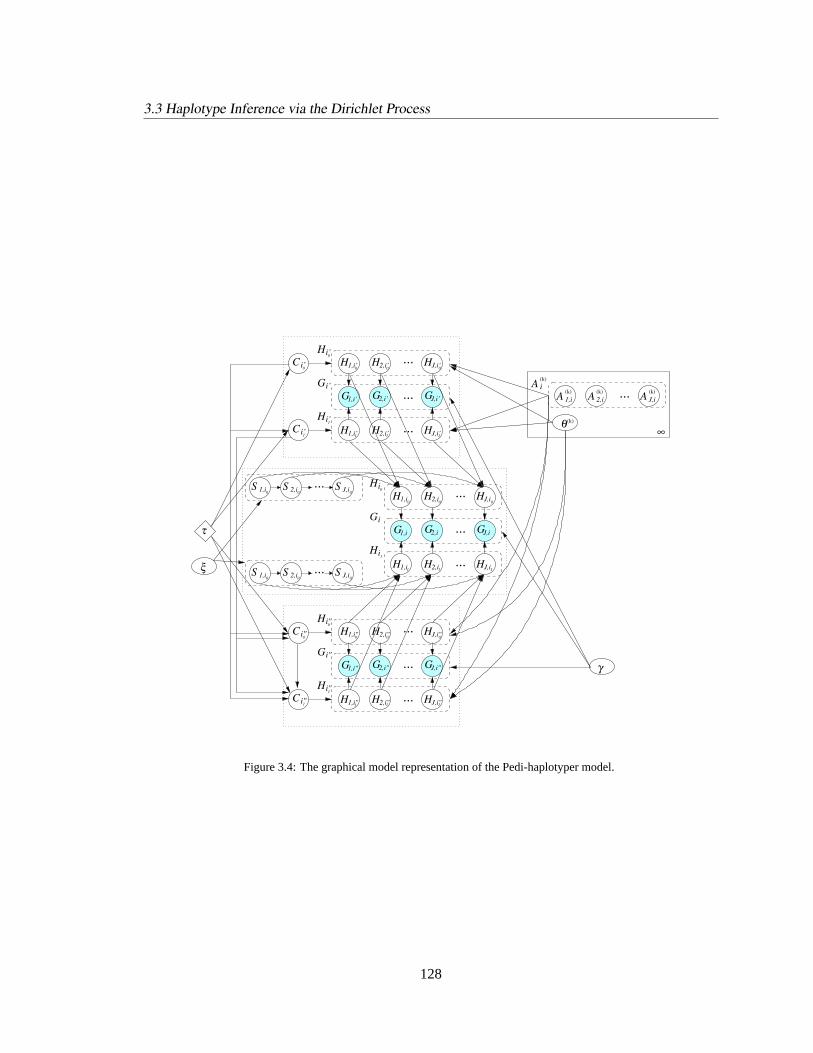
3.3 Haplotype Inference via the Dirichlet Process
H1,i1 H2,i1 HJ,i1
G1,i G2,i GJ,i
Hi1
Gi
Hi0
H1,i0 H2,i0HJ,i0
...S 1,i0S 2,i0
S J,i0
S 1,i0S 2,i0
S J,i0
...
H1,i’1 H2,i’1 HJ,i’1
G1,i’ G2,i’ GJ,i’
Hi’1
Gi’
Hi’0
C i’1
H1,i’0 H2,i’0 HJ,i’0
H1,i"1 H2,i"1 HJ,i"1
G1,i" G2,i" GJ,i"
Hi"1
Gi"
Hi"0
C i"1
C i"0 H1,i"0 H2,i"0 HJ,i"0
A 2,i(k) A J,i
(k)A i
(k)
A 1,i(k)
∞
...
θ(k)
γ
τ
C i’0
ξ
...
...
...
...
...
...
...
...
...
Figure 3.4: The graphical model representation of the Pedi-haplotyper model.
128

3.3 Haplotype Inference via the Dirichlet Process
the maternal allele of individuali’s t-parent (wheret = 0 means father andt = 1 means mother).
We denote thet-parent of individuali byπ(it), and his/her paternal (resp. maternal) allele byπ0(it)
(resp. π1(it)). We use the following conditional distribution to model possible mutation during
single generation inheritance.
p(hit,j |sit,j = r, hπ0(it),j , hπ1(it),j , εt) =[εt]I(hit,j=hπr(it),j
)[ 1− εt|B| − 1
]I(hit,j 6=hπr(it),j),(3.11)
where1 − εt is the mutation rate during inheritance, andr ∈ 0, 1 represents the choice of the
paternal or maternal alleles of a parent subject by an offspring. Note that thissingle generation
inheritance modelallows different mutational rates for the parental and maternal alleles if desired
(e.g., to reflect the difference in gamete environment in a male or a female body), by lettingε0 and
ε1 take different values, or giving them different beta prior distributions in case we want to model
uncertainty ofεt in a Bayesian framework.
To model possible recombination events during single generation inheritance, we assume that
the list of segregation random variables,[Sit,1, . . . , Sit,J ], associated with individual haplotypeHit ,
forms a 1st-order Markov chain, with transition matrixξ:
p(Sit,j+1 = r′|Sit,j = r) = ξrr′
=[ξ]I(r=r′)[1− ξ
]I(r 6=r′), (3.12)
where1− ξ is the probability of a recombination event (i.e., a swap of parental origin) at positionj.
This model is equivalent to assuming that the recombination events follow a Poisson point process
of rate ξ along the chromosome. If desired, a beta priorBeta(αs, βs) can be introduced forξ.
Again, the recombination rates in males and females can be different if desired.
Looking back to the overall graphical topology of the Pedi-haplotyper model, as illustrated
in Figure3.4, for founding members in the pedigree (i.e., those without parental information), or
half founding members (i.e., those with information from only one of the two parents), we assume
that their un-progenitored haplotype(s) are inherited from some ancestors, thus following the basic
haplotype model described in§3.3. For the haplotypes of the offspring in the pedigree, we couple
129

3.4 Experimental Results
them to their parents using the single generation mutation and recombination model described in the
previous paragraphs. Thus, the Pedi-haplotyper model proposed in this section is fully generalizable
to any pedigree structure.
Solving the Pedi-haplotyper model is slightly more difficult than for the basic Dirichlet process
mixture model, DP-haplotyper, foriid populations. But as we show in Chapter 5, most of the
methods we developed for the DP-haplotyper can be directly used in this more elaborate framework,
with the addition of a few new sampling steps for the newly introduced random variables.
3.4 Experimental Results
We validated our algorithm by applying it to simulated and real data and compared its performance
to that of the state-of-the-art PHASE algorithm[Stephenset al., 2001] and other current algorithms.
We report on the results of both variants of our algorithm: the Gibbs sampler, denoted DP(Gibbs),
and the Metropolis-Hasting sampler, denoted DP(MH). Throughout the experiments, we set the
hyperparameterτ in the Dirichlet process to be roughly1% of the population size, i.e., for a data
set of 100 individuals,τ = 1. We used a burn-in of 2000 iterations (or 4000 for datasets with more
than 50 individuals), and used the next 6000 iterations for estimation.
3.4.1 Simulated Data
In our first set of experiments we applied our method to simulated data (“short sequence data”)
from Stephenset al. [2001]. This data contains sets of2n haplotypes, randomly paired to form
n genotypes, under an infinite-sites model with parametersη = 4 andR = 4 determining the
mutation and recombination rates, respectively. We used the first 40 datasets for each combination
of individuals and sites, where the number of individuals ranged between 10 and 50, and the number
of sites ranged between 5 and 30.
To evaluate the performance of the algorithms we used the following error measures:errs, the
ratio of incorrectly phased SNP sites over all non-trivial heterozygous SNPs (excluding individu-
als with a single heterozygous SNP);erri, the the ratio of incorrectly phased individuals over all
130

3.4 Experimental Results
DP(MH) PHASE EM#individuals errs erri ds errs erri ds erri
10 0.060 0.216 0.051 0.046 0.182 0.054 0.42420 0.039 0.152 0.039 0.029 0.136 0.046 0.29630 0.036 0.121 0.038 0.024 0.101 0.027 0.23140 0.030 0.094 0.029 0.019 0.071 0.026 0.19550 0.028 0.082 0.024 0.019 0.072 0.025 0.167
Table 3.1: Performance on data fromStephenset al. [2001]. The results for the EM algorithm are adapted fromStephenset al. [2001].
non-trivial heterogeneous individuals; andds, the switch distance, which is the number of phase
flips required to correct the predicted haplotypes over the total number of non-trivial heterogeneous
SNPs. The results are summarized in Table3.1. Overall, we perform slightly worse than PHASE
on the first two measures, and slightly better on the switch distance measure (which uses 100,000
sampling steps). Both algorithms provide a substantial improvement over EM.
DP(Gibbs) DP(MH) PHASE HAP HAPLOTYPERblockid.
length errs erri ds errs erri ds errs erri ds errs errs
1 14 0.223 0.485 0.229 0 0 0 0.003 0.030 0.003 0.007 0.0392 5 0 0 0 0.007 0.026 0.007 0.007 0.026 0.007 0.036 0.0653 5 0 0 0 0 0 0 0 0 0 0 0.0084 11 0.143 0.262 0.128 0 0 0 0 0 0 0.015 -5 9 0.020 0.066 0.020 0.011 0.033 0.011 0.011 0.033 0.011 0.027 0.1516 27 0.071 0.191 0.074 0.005 0.043 0.005 0 0 0 0.018 0.0417 7 0.005 0.018 0.005 0.005 0.018 0.005 0.005 0.018 0.005 0.068 0.2148 4 0 0 0 0 0 0 0 0 0 0 0.2529 5 0.029 0.097 0.029 0.012 0.032 0.012 0.012 0.032 0.012 0.057 0.15210 4 0.007 0.025 0.007 0.007 0.025 0.007 0.008 0.025 0.008 0.042 0.05611 7 0.010 0.034 0.005 0.005 0.017 0.005 0.011 0.034 0.011 0.033 0.09312 5 0.010 0.037 0.020 0 0 0 0 0 0 0 0.077
Table 3.2: Performance on the data ofDaly et al.[2001], using the block structure provided byHalperin and Eskin[2002].The results of HAP and HAPLOTYPER are adapted fromHalperin and Eskin[2002]. Since the error rate inHalperinand Eskin[2002] uses the number of both heterozygous and missing sites as the denominator, whereas we used only thenon-trivial heterozygous ones, we rescaled the error rates of the two latter methods to be comparable to ours.
3.4.2 Real Data
We applied our algorithm to two real datasets and compared its performance to that of PHASE
[Stephenset al., 2001] and other algorithms.
The first dataset contains the genotypes of 129 individuals over 103 polymorphic sites[Daly et
al., 2001]. In addition it contains the genotypes of the parents of each individual, which allows the
131

3.4 Experimental Results
1 2 3 4 5 6 7 8 9 100
50
100
150 112.3680 42.8975 24.0215 15.8180 11.4060 8.5905 6.6175 5.2755 4.2945 3.5750
1 2 3 4 5 6 7 8 9 100
50
100
150 155.9960 61.1640 33.7340 4.9460 2.0220 0.1100 0.0220 0.0060
0 0
1 2 3 4 5 6 7 8 9 100
50
100
150 154.8800 62.8620 33.2480 4.9700 2.0000 0.0400
0 0 0 0
Figure 3.5: The top ten ancestral templates during Metropolis-Hasting sampling for block 1 of the data of[Daly et al.,2001]. (The numbers in the panels are the posterior means of the frequencies of each template). (a) Immediately afterburn-in (first 2000 samples). (b) 3000 samples after burn-in. (c) 6000 samples after burn-in.
inference of a large portion of the haplotypes as inEskinet al.[2003]. The results are summarized in
Table3.2. It is apparent that the Metropolis-Hasting sampling algorithm significantly outperforms
the Gibbs sampler, and is to be preferred given the relatively limited number of sampling steps (∼
6000). The overall performance is comparable to that of PHASE and better than both HAP[Halperin
and Eskin, 2002; Eskinet al., 2003] and HAPLOTYPER[Niu et al., 2002].
It is important to emphasize that our methods also providea posterioriestimates of the ancestral
pool of haplotype templates and their frequencies. We omit a listing of these haplotypes, but provide
an illustrative summary of the evolution of these estimates during sampling (Figure3.5).
The second dataset contains genotype data from four populations, 90 individuals each, across
several genomic regions[Gabrielet al., 2002]. We focused on the Yoruban population (D), which
contains 30 trios of genotypes (allowing us to infer most of the true haplotypes) and analyzed the
genotypes of 28 individuals over four medium-sized regions (see below). The results are summa-
rized in Table3.3. All methods yield higher error rates on these data, compared to the analysis of
the data ofDaly et al. [2001], presumably due to the low sample size. In this setting, over all but
one of the four regions, our algorithm outperformed PHASE for all three types of error measures. A
preliminary analysis suggests that our performance gain may be due to the bias toward parsimony
induced by the Dirichlet process prior. We found that the number of template haplotypes inferred in
our algorithm is typically small, whereas in PHASE, the hypothesized haplotype pool can be very
large (i.e., region 7b has 83 haplotypes, compared to 10 templates in our case and 28 individuals
overall).
132

3.5 Conclusions and Discussions
DP(MH) PHASEregion length errs erri ds errs erri ds
16a 13 0.185 0.480 0.141 0.174 0.440 0.1301b 16 0.100 0.250 0.160 0.200 0.450 0.18025a 14 0.135 0.353 0.115 0.212 0.588 0.2127b 13 0.105 0.278 0.066 0.145 0.444 0.092
Table 3.3: Performance on the data ofGabrielet al. [2002].
0 1000 2000 3000 4000 5000 6000 7000 80000
10
20
30
40
50
60
# of samples
# of
anc
estra
l tem
plat
es
Figure 3.6: Sampling trace of the number of population haplotypes derived from the genotypes. As can be seen, theMarkov chain starts from a rather non-parsimonious estimation, and converges to a parsimonious solution after about twothousand samples.
In terms of computational efficiency, we noticed that PHASE typically required 20,000 to
100,000 steps until convergence, while our DP-based method required around 2,000∼6,000 steps
to convergence (Fig.3.6).
3.5 Conclusions and Discussions
In this chapter, we have proposed a Bayesian approach to the modeling of genotypes based on a
Dirichlet process prior. We have shown that the Dirichlet process provides a natural representation
of uncertainty regarding the size and composition of the pool of haplotypes underlying a population.
We will present in Chapter 5 several Markov chain Monte Carlo algorithms for haplotype inference
under either a basic DP mixture haplotype model intended for aniid population, or, an extended
graphical DP mixture model — Pedi-haplotyper model — for a population containing bothiid sub-
jects and subjects coupled by partial pedigrees. The experiments on the basic DP mixture haplotype
model show that this model leads to effective inference procedures for inferring the ancestral pool
133

3.5 Conclusions and Discussions
and for haplotype phasing based on a set of genotypes. The model accommodates growing data col-
lections and noisy and/or incomplete observations. The approach also naturally imposes an implicit
bias toward small ancestral pools during inference, reminiscent of parsimony methods, doing so in
a well-founded statistical framework that permits errors.
Our focus here has been on adapting the technology of the Dirichlet process to the setting of
the standard haplotype phasing problem. But an important underlying motivation for our work, and
a general motivation for pursuing probabilistic approaches to genomic inference problems, is the
potential value of our model as a building block for more expressive models. In particular, as in
Greenspan and Geiger[2003] andLauritzen and Sheehan[2002], the graphical model formalism
naturally accommodates various extensions, such as segmentation of chromosomes into haplotype
blocks and the inclusion of pedigree relationships. In section§3.4, we have outlined a preliminary
extension of the basic Dirichlet process mixture model that incorporates pedigree relationships and
briefly discussed how to model realistic biological processes that might influence haplotype forma-
tion and diversification, such as recombination and mutation during single generation inheritance.
We recognize that many other important issues also deserve careful attention, for example, haplo-
type recombinations among the ancestral haplotype pools (so far, we assume that these ancestral
haplotypes relate to modern individual haplotypes only via mutations), aspects of evolutionary dy-
namics (e.g., coalescence, selection, etc.), and linkage analysis under joint modeling of complex
traits and haplotypes. We believe that the graphical model formalism we proposed can readily
accommodate such extensions. In particular, it appears reasonable to employ an ancestral recombi-
nation hypothesis (rather than single generation recombination) to account for common individual
haplotypes that are distant from any single ancestral haplotype template, but can be matched piece-
wise to multiple ancestral haplotypes. This may be an important aspect of chromosomal evolution
and can provide valuable insight into the dynamics of populational genetics in addition to point-
mutation-based coalescence theory, and can potentially improve efficiency and quality of haplotype
inference.
134

3.5 Conclusions and Discussions
The Dirichlet process parameterization also provides a natural upgrade path for the consider-
ation of richer models; in particular, it is possible to incorporate more elaborate base measuresG
into the Dirichlet process framework—the coalescence-based distribution ofStephenset al. [2001]
would be an interesting choice. In Chapter 5, while developing MCMC algorithms for haplotype in-
ference, we will also briefly discuss a heuristic for constructing an informative base measure for the
DP using low-quality but inexpensive haplotype information (e.g., that obtained from a conventional
EM algorithm). Note that the partition structure of the Dirichlet process is equivalent to that induced
by the Ewens sampling formula (ESF)[Tavare and Ewens, 1998] known to the population genetics
community. The ESF represents a non-Darwinian theory of evolution which claims that “the exten-
sive genetic variation observed in natural populations is, on the whole, not due to natural selection,
but arises rather as a result of purely stochastic changes in gene (allele) frequencies in a finite pop-
ulation” [Tavare and Ewens, 1998]. The fact that our DP mixture model performed adequately in
a number of problems suggests that such non-Darwinian evolution may apply to SNP distribution,
which is interesting, yet would appear paradoxical, if we proceed to use haplotypes to map clearly
non-neutral genes (say, those that relate to biological disorders) via linkage disequilibrium.
135

Chapter 4
Probabilistic Inference I: DeterministicAlgorithms
The Bayesian graphical models presented in the last two chapters both define high-dimensional,
hybrid probability distributions for which important statistical queries may be difficult to compute.
For example, in theLOGOS model, the sequence variableYt at sitet of a study sequence depends on
all the motif parametersθ(k)
l |∀l, k, each of which in turn depends on one of the PSMD prototype
(i.e., Dirichlet component) indicatorsS(k)
l |∀l, k coupled by a first-order Markov chain. Thus, to
compute the posterior probability distributionsp(xt|y) andp(θ(k)
l |y) for MAP prediction of motif
locations and Bayesian estimation of motif PWMs, one has to integrate over the Cartesian product
of a continuous state space for the PWMs and the discrete spaces for the PSMD prototype (denoted
asD) and for the sequence annotation indicators (denoted asS). The complexity of such a state
space is on the order of
R4×P
k Lk × |D|P
k Lk × |S|T ,
which translates toO(R120 × 101000) for a 1000 bp sequence harboring only two possible motif
patterns each of length 15 bp. Clearly, this computation is in general intractable with any off-the-
shelf exact algorithm and some approximation scheme is necessary. In this chapter, we present a
general variational approach for computing deterministic approximations to such intractable dis-
tributions. In the next chapter, we briefly discuss stochastic approximation methods based on
sampling. Some of the materials covered in this chapter have appeared in[Xing et al., 2003b;
136

4.1 Background
Xing et al., 2004a].
4.1 Background
For a multivariate probability distributionp(xH ,xE), whereXH andXE denote the sets of all un-
observed (i.e., hidden) and observed (i.e., evidence) variables, respectively (and, following conven-
tion, their lower case counterparts denote states or values of the corresponding variables), the gen-
eral problem of probabilistic inference is that of computing the conditional probabilitiesp(xF |xE),
whereF ⊆ H is the index set of an arbitrary subset of hidden variables.
Probabilistic inference techniques play an important role in any probabilistic methodology for
prediction and learning. For example, probabilistic prediction of unobserved events or patterns
in real world tasks such as weather forecasting, text segmentation and tagging, robot localization,
image analysis, filtering and smoothing of sequential data streams, and various computational biol-
ogy problems such as motif, haplotype and pedigree inference considered in this thesis, all involve
performing probabilistic inference on a domain-specific, high-dimensional, and often hybrid (i.e.,
comprising both discrete and continuous variables) probability model. Probabilistic inference is
also indispensable for the acquisition of probability models from incomplete or partially observed
data using statistical learning methods, because many of these methods amount to parameter estima-
tion based on a maximum likelihood or an empirical Bayes principle[Efron, 1996], which employs
an inference subroutine to impute the unobserved variable(s) for computing the necessary sufficient
statistics.
Solving an inference query can be understood as amarginalizationcomputation. To see this,
observe that the conditional probabilityp(xF |xE) is equal to:
p(xF |xE) =p(xF ,xE)p(xE)
=
∑xH\F
p(xH\F ,xF ,xE)∑xFp(xF ,xE)
, (4.1)
where the summation (or integration in case of continuous variables) over all possible values of
some (or all) hidden variables in the model is calledmarginalization. Typically, an inference query
involves computing the conditional probabilities for only small subsets of variables (e.g., that of
137

4.1 Background
singleton hidden variables such asxt in the LOGOS model), and sometimes a large number of
such queries need to be processed (e.g., allxt’s for motif detection underLOGOS). This is often
a computationally expensive operation, as the state space to be swept during marginalization grows
exponentially with the number of variables being marginalized. The graphical model formalism
provides a systematic and efficient approach to such computation. General exact inference algo-
rithms have been developed, which take advantage of the conditional independencies present in the
joint distributionp(xH ,xE), which can be inferred from the pattern of missing edges in the graph,
to distribute the high-dimensional combinatorial summation over all hidden variables in a standard
marginalization operation into a sequence of low-dimensional local summations each over a (small)
subset of hidden variables (Fig.4.1). We will briefly describe a representative of these algorithms,
the junction tree algorithm, in the next section.
X1
X2
X3
X6
X5X4
Figure 4.1: Inference on a graphical model. The dark shading indicates the node on which we condition, the unshadednode is the one for which we wish to compute the conditional probability distribution, and the lightly shaded nodes arethose that need to be marginalized out in computing the posterior probabilityp(x1|x6). For this graphical model, the sum-mations for computing the joint marginal can be distributed to subsets of variables in the following way (formally knownas anelimination algorithm): p(x1, x6) =
Px2,x3,x4,x5
p(x1)p(x2|x1)p(x4|x1)p(x3|x2)p(x5|x4)p(x6|x2, x5) =p(x1)
Px2
p(x2|x1)P
x3p(x3|x2)
Px4
p(x4|x1)P
x5p(x5|x4)p(x6|x2, x5)
.
Although there are many cases in which the exact algorithms provide a satisfactory solution
to the inference and learning problems, large-scale probability models arising from complex real
world domains have outgrown the ability of current (and probably future) exact inference algorithms
to compute marginals and learn parameters. This is particularly true for models we developed
in this dissertation, which concern complex gene regulation elements and genetic polymorphism
patterns in the genomic sequences. As illustrated at the beginning of this chapter, the time and
138

4.1 Background
space complexity of the exact algorithms is unacceptable and it is necessary to have recourse to
approximation procedures.
For this reason, the development of efficient and broadly applicable approximation algorithms
for probabilistic inference is critical to further progress. Two commonly used approximation tech-
niques areMonte Carlomethods (such as Markov chain Monte Carlo, or MCMC) andvariational
methods. MCMC techniques are asymptotically exact and easy to apply. The BUGS system uses
MCMC within a general-purpose statistical modeling language (see[Gilks et al., 1996]), and the
inference process can be set up automatically for a variety of models. Unfortunately, MCMC often
converges very slowly. Variational methods, on the other hand, are claimed to exhibit fast conver-
gence and (in some cases) give a deterministic lower bound on the true likelihood. The original
belief propagation (BP) method[Pearl, 1988] is now understood as a variational algorithm[Yedidia
et al., 2001b] that (if it converges) calculates an optimal approximation to the true posterior dis-
tribution among those approximate distributions that include onlypairwisedependencies among
variables. BP can be applied straightforwardly to a wide range of probability models and it has been
used for biological classification/clustering problems expressed as complex graphical models[Se-
gal et al., 2001]. A generalized BP (GBP) algorithm can be derived that operates with dependency
structures on larger clusters of variables and often gives more accurate results[Yedidiaet al., 2001a]
1. Like BP, GBP sometimes fails to converge. It may also fail to give a lower bound on the true
likelihood due to the use of anad hocapproximation to the intractable entropy term in the objective
functional it optimizes (to be detailed in§4.3.4.3). Other variational approximation methods based
on structured mean field approximation have been developed that are guaranteed to converge to
lower bounds on the true likelihood (see, e.g.,[Jordanet al., 1999]), but these methods often require
model-specific derivation of iteration equations.
In this chapter, we develop a generalized mean field (GMF) theory which leads to a generic
variational inference algorithm that is straightforwardly applicable to a wide range of models and is
guaranteed to converge to a lower bound on the true likelihood. Given an arbitrary decomposition of
1Similar techniques called cluster variational methods (CVMs) have also been developed in the statistical physicscommunity[Kappen and Wiegerinck, 2002].
139

4.1 Background
the original model into disjoint clusters of variables, the algorithm computes the posterior marginal
for each cluster given its own evidence and theexpected sufficient statistics, obtained from its neigh-
boring clusters, of the variables in the cluster’s Markov blanket. Optimal clustering of the variables
can be obtained in a principled fashion via a graph partition algorithm. The algorithm operates in
an iterative, message-passing style until a fixed point is reached. We show that the cluster marginals
retain exactly the intra-cluster dependencies of the original model, which means that the inference
problem within each cluster can be solved independently of the other clusters (given the Markov
blanket messages) by any inference method. This GMF algorithm is applied to the Bayesian motif
prediction and learning problem under theLOGOS model and shows significant improvement over
a sampling-based approach (discussed in the next chapter).
4.1.1 Notation
Before starting the technical sections, here is a summary of some necessary notations and definitions
needed in our exposition.
We consider a graph (directed or undirected)G(V, E), whereV denotes the set of nodes (ver-
tices) andE the set of edges (links) of the graph. LetXn denote the random variable associated
with noden, for n ∈ V; let XC denote the subset of variables associated with a subset of nodesC,
for C ⊆ V, and letX = XV denote the collection of all variables associated with the nodes of the
graph. We use upper-caseX (resp.X) to denote a random variable (resp. variable set), and lower-
casex (resp.x) to denote a certain state (or value, configuration, etc.) taken by the corresponding
variable (resp. variable set). We refer to a graphH = (V, E ′), whereE ′ ⊆ E , as asubgraphof G.
We useC = C1, C2, . . . , CI to denote a disjoint partition (or, aclustering) of all nodes in graph
G, whereCi refers to the set of indices of nodes in clusteri; likewise,D = D1, D2, . . . , DK
denotes a set ofcliques(i.e., completely connected subsets of nodes) ofG. For a given clustering,
we define theborder clique setBi as the set of cliques that intersect with but are not contained in
clusteri; and theneighbor cluster setNi as the set of clusters that contain nodes connected to nodes
in clusteri. For undirected graphs, theMarkov blanketof a clusteri (MBi) is the set of all nodes
140

4.2 Exact Inference Algorithms
outsideCi that connect to some node inCi, and, for directed graphs, the Markov blanket is the set
of all nodes outsideCi that are parents, children, or co-parents (other than those already inCi) 2 of
some node inCi (Fig. 4.2). Clusters that intersect withMBi are called theMarkov blanket clusters
(MBCi) of Ci.
...y11
y12 y13
y14
y15y16
...y71
y72 y73
y74
y75y76
...y21
y22 y23
y24
y25y26
...y61
y62 y63
y64
y65y66
...y51
y52 y53
y54
y55y56
...y
y42 y43
y44
y45y46
41
...y31
y32 y33
y34
y35y36
C1
Figure 4.2: The Markov blanketMB1 (blue-shaded nodes) of cluster1 in a directed graph. Shaded blobs constituteMBC1.
4.2 Exact Inference Algorithms
In this section, we give a brief overview of the junction tree algorithm[S. Lauritzen, 1988]. It is a
general purpose algorithm which subsumes many other exact inference inference algorithms (e.g.,
belief propagation for tree models[Pearl, 1988], the forward-backward algorithms for HMMs[Ra-
biner and Juang, 1986], the peeling algorithm for pedigree models[Thompson, 1981], etc.) as
special cases.
4.2.1 The Junction Tree Algorithm
As described in Chapter 1, for a directed graphical modelG(V, E), the joint probability distribution
for all the |V| nodes in the graph can be written as the product of alllocal conditional distributions
defined on each node and its parent(s):
p(x) =|V|∏i=1
p(xi|xπi). (4.2)
2A co-parent of a node, say,Xv, is defined as the parent (other thanXv) of a child nodeXu of Xv.
141

4.2 Exact Inference Algorithms
For an undirected graphical model, the joint probability distribution is equal to the product of the
potential functionsassociated with each clique of the graph, up to a normalization constant:
p(x) =∏|D|
α=1 φα(xDα)Z
, (4.3)
whereZ =∑
x
∏|D|α=1 φα(xDα) is referred to as a “partition function”.
X1
X2
X3
X6
X5X4
⇒X1
X2
X3
X6
X5X4
Figure 4.3: Moralization of a directed graph.
A directed graphical model can be converted into an equivalent undirected graphical model via
an operation called “moralization,” which connects all parents of a common child node pairwise
with undirected edges, and then drops the directionality of all other edges in the graph (Fig.4.3).
The resulting graph is called a “moral graph,” in which all the nodes originally involved in a local
conditional distribution in the directed graph now appear together in a common clique. Thus, local
conditional distributions in a directed graph can be thought of as normalized potential functions
in the corresponding moral graph, and the product rule (i.e., Eq. (4.2) and Eq. (4.3)) of the joint
distribution gives the same outcome for the directed model and its undirected counterpart. Due to
the equivalence of the undirected moral graph to the original directed graph in representing a joint
probability distribution, the junction tree algorithm concerns only undirected graphs.
The junction tree algorithm starts with the moralized graph. It first chooses anelimination order
for all nodes in the graph, and applies an operation calledtriangulation to this order as follows: 1)
choose the next node in the elimination order, 2) add edges to link all remaining pairs of nodes
that are neighbors of this node and, 3) remove the node (and all its incident edges) from the graph.
Taking the new edges added in this process and adding them to the original moralized graph yield a
triangulated graph(Fig. 4.4a).
142

4.2 Exact Inference Algorithms
A triangulated graph allows the creation of a data structure known as ajunction tree(Fig. 4.4b),
on which a generalized message-passing algorithm can be defined. A full discussion of the con-
struction of a junction tree is beyond the scope of this thesis; in short, it is a maximal spanning
tree of cliques in the triangulated graph, with weights defined by the cardinality of the intersections
between cliques. A key property of the junction tree is the so calledrunning intersection property,
which says that if a node appears in any two cliques in the tree, it appears in all cliques that lie on
the path between the two cliques. As a consequence of this property, in a junction tree, local con-
sistency (i.e., potentials ofadjacent cliques in the tree agree on marginals of any shared variables)
implies global consistency (i.e., potentials ofall cliques in the tree agree on marginals of common
variables).
X1
X2
X6
X5X4
X3
X1 X2 X4, , X2 X4 X5, , X2 X5 X6, ,X2 X5,
X2 X3,
X2 X4,
X2
(a) (b)
Figure 4.4: Construction of the junction tree. (a) The triangulated graph of the graphical model in Fig.4.3. (b) Thejunction tree. Squares represent original cliques in the triangulated graph, ellipsoids represent separators of adjacentcliques.
With the junction tree, the joint probability distribution can now be expressed in the following
factored form:
p(x) =
∏Ci∈CT
ψi(xCi)∏Sj∈ST
φj(xSj ), (4.4)
whereCT is the set of all cliques in the triangulated graph andST is the set of separators (i.e., clique
intersections) spanned by the junction tree.
143

4.2 Exact Inference Algorithms
The clique potentialsψ(·) and separator potentialsφ(·) can be updated by running a message-
passing protocol on the junction tree, with the following update rule:
φ∗j (xSj ) =∑
xCi\Sj
ψi(xCi), ψ∗k(xCk) =
φ∗j (xSj )φj(xSj )
ψk(xCk),
whereXSj denotes the set of variables that separates cliquesXCi andXCj , and the “message”
is now passed from cliquei to cliquek via separatorj (Fig. 4.5). The protocol typically starts
by picking a root of the tree, and then first passing messages from root to all leaves along tree
branches, and then collecting messages from all leaves to the root, which leads toψi = p(xCi) and
φj = p(xSj ) for all i, j, when the message passing terminates. Note that a single run of the junction
tree algorithm yields all clique marginals, not merely that corresponding to a single clique.
X1 X2 X4, , X2 X4 X5, , X2 X5 X6, ,X2 X5,
X2 X3,
X2 X4,
X2
iX kXjX
Figure 4.5: Message passing in a junction tree.
It is easy to see that the computational bottleneck of the junction tree algorithm is determined
by the size of the maximal clique in the triangulated graph, which is affected by the choice of the
elimination order that induces the triangulated graph. The minimum of the maximal clique size
among all possible triangulations is know as thetree widthof the graph. Choosing an elimination
order that minimizes the maximal clique size is non-trivial (indeed, it is an NP-hard problem for
arbitrary graphs, but can often be effectively approached on special graphs). There are many special-
purpose exact inference algorithms for specific families of graphical models (e.g., the forward-
backward algorithm for HMMs, Pearl’s belief propagation algorithm for trees, etc.), almost all of
which are essentially special cases of the the junction tree algorithm applied to special graphs, using
a special and often optimal choice of the elimination order for triangulation.
144

4.3 Approximate Inference Algorithms
4.3 Approximate Inference Algorithms
As mentioned, for a complex distribution, computing the marginal (or conditional) distributions,
as well as the maximuma posterioriconfigurations, of an arbitrary subset of the random variables
is intractable. The variational approach to these inference problems involves converting them into
an optimization problem, then approximating the feasible set of the solution or the function to
be optimized (or both), and solving the relaxed optimization problem. Thus, given a probability
distributionp(x|θ) that factors according to a graph, the variational methods yield approximations
to marginal probabilities via the solution to an optimization problem that generally exploits some
of the graphical structure. In the sequel, we describe a general variational principle for inference
in probabilistic graphical models, on which a variety of extant deterministic approximate inference
techniques are based, and from which we draw the mathematical foundations for the subsequent
development of a more general approach for approximate inference called generalized mean field
(GMF) inference. We begin with some necessary definitions and algebraic preliminaries.
4.3.1 Cluster-factorizable Potentials
Given a clusteringC of all nodes inG(V, E), some cliques inD may intersect with multiple
clusters (Fig.4.6). Cluster-factorizable potentialsare potential functions which take the form
φβ(xDβ) = Fβ(φβi
(xDβ∩Ci), . . . , φβj
(xDβ∩Cj)), whereF (·) is a (multiplicatively, or additively)
factorizable function over its arguments; i.e., in the case of two clusters,F (a, b) = a × b or a + b.
Factorizable potentials are common in many model classes. For example, the classical Ising model
is based on singleton and pairwise potentials of the following factorizable form (under the expo-
nential representation, as described shortly):φ(xi) = θixi, φ(xi, xj) = θijxixj ; higher-order Ising
models and many more general discrete models also admit factorizable potentials; conjugate expo-
nential pairs, such as the Dirichlet-multinomial, linear-Gaussian, etc., are also factorizable; finally,
for logistic functions and other generalized linear models (GLIMs) that are not directly factorizable,
it is often possible to obtain a factorizable variational transformation in the exponential family that
145

4.3 Approximate Inference Algorithms
lower bounds the original function[Jaakkola and Jordan, 2000]. In other cases (e.g., tabular poten-
tials over a clustering of variables), a more general treatment based on peripheral marginal potentials
can be used (see§4.4.3). We will see that cluster-factorizable potentials allow the decoupling of the
computation of expected potentials.
Ci
Ck
Cl
Dβ
Figure 4.6: A cliqueDβ intersecting with three clustersCi, Cj , Ck in an undirected graph.
4.3.2 Exponential Representations
In order to formulate variational inference as a generic optimization problem, it is convenient to use
the following exponential representation for a graphical model.
Similar to the general parameterization of graphical models introduced in Chapter 1, under
exponential representations, for undirected graphical models, the family of joint probability distri-
butions associated with a given graph can be parameterized in terms of a set ofpotential functions
associated with a set of cliques in the graphs3. For a set of cliquesD = Dα|α ∈ A associated
with an undirected graph, indexed by a setA, let φ = φα|α ∈ A denote the set of potential
functions defined on the cliques, andθ = θα|α ∈ A the set of parameters associated with these
potential functions (for simplicity, we labelφ andθ with the correspondingclique index, e.g.,α,
rather than with the cliqueDα itself). The family of joint distributions determined byφ can be
3More precisely, these potential functions are nowexponential potential functionsthat are semantically different fromwhat we meant by “potential functions” in our early exposition of graphical models. Technically, however, little differenceexists in their definitions, except that the range of the exponential potential functions is all real numbers whereas theoriginal potential functions have positive values. For fixed potential weights, there exists a one-to-one correspondencebetween the two types of potential functions. For simplicity, in the sequel we still use the term “potential functions” inour exposition under the exponential representations.
146

4.3 Approximate Inference Algorithms
expressed as follows:
p(x|θ) = exp∑α∈A
θαφα(xDα)−A(θ) (4.5)
whereA(θ) is thelog partition function. We also define theenergy,E(x) = −∑
α θαφα(xDα), for
statex.
For directed graphical models, in which the joint probability is defined asp(x) =∏
i p(xi|xπi),
we transform the underlying directed graph into amoral graph, and set the potential functions
φi(xi,xπi) equal to the logarithms of the local conditional probabilitiesp(xi|xπi). In the sequel, we
will focus on models based onconditional exponential families. That is, the conditional distributions
p(xi|xπi) can be expressed as:
p(xi|xπi) = u(xi) expθTi φi(xi,xπi)−A(θi,xπi), (4.6)
whereφi(xi,xπi) is a vector of potentials associated with the variable setxi,xπi.
The exponential representation applies to a wide range of models of practical interest, including
discrete models, Gaussian, Poisson, exponential, and many others.
4.3.3 Lower Bounds of General Exponential Functions
Now we review some basic results from standard calculus that provide a principled way of con-
structing higher-order bounds for regular functions. Start from a simple bound for a functionf0(x):
f0(x) ≥ b0(x),∀x ∈ X .
Lemma 1 For anti-derivativesf1(x) off0 andb1(x) of b0 such thatf1(a) = b1(a) for somea ∈ X :
f1(x) ≤ b1(x) for x ≤ a
f1(x) ≥ b1(x) for x ≥ a
Proof. Due to the simple bound assumption, forx ≥ a:∫ x
adzf0(z) ≥
∫ x
adzb0(z)
⇒ f1(x)− f1(a) ≥ b1(x)− b1(a)
⇒ f1(x)− b1(x) ≥ f1(a)− b1(a) = 0.
147

4.3 Approximate Inference Algorithms
The other direction (i.e., whenx ≤ a) follows similarly.
Lemma 2 For anti-derivativesf2(x) of f1 andb2(x) of b1 such thatf2(a) = b2(a), f1(a) = b1(a):
f2(x) ≥ b2(x) for x ∈ X
Proof. Due to Lemma1, for x ≤ a:∫ a
x
dzf1(z) ≤∫ a
x
dzb1(z)
⇒ f2(x)− b2(x) ≥ f2(a)− b2(a) = 0
Forx ≥ a, the same inequality follows similarly.
Thus we have the following theorem:
Theorem 1 Let fk(x) denote thekth-order anti-derivative of the functionf(x). Given a lower
boundb(x) of the functionf(x), the 2nd-order anti-derivativeb2(x) of the original bound, parame-
terized by a variational parameterµ such thatb1(µ) = f1(µ) andb2(µ) = f2(µ), is a lower bound
of f2(x). Likewise (by induction), bounds for higher-order anti-derivatives off can be successively
constructed.
Since the anti-derivative of the exponential function is just itself, we can easily use Theorem1
to obtain linear and higher-degree polynomial bounds from bounds of lower order. For example,
the well known linear bound of the exponential function, its tangent atx = µ (see Fig4.7), can be
readily derived from the trivial boundexp(x) > 0 using Theorem1:
f(x) = exp(x) ≥ exp(µ)(1 + x− µ) = b2(x),∀x, µ (4.7)
Integrating over both sides twice, and denoting the variational parameters in the new bound
asν (which means that new bound “touches” the original function atν), we have the following
third-order bound:
f(x) = exp(x)
≥ exp(ν)1 + x− ν + exp(ξ)
(1− ξ
2(x− ν)2 +
16(x− ν)3
),
= b4(x). (4.8)
148

4.3 Approximate Inference Algorithms
whereξ = µ − ν. Whenξ = 0, that is, restricting the higher order bound to “touch” the original
function at the same point as the lower order bound, we haveb4(x) = 16 exp(µ)((x−µ)3 +3(x−µ)2 +
6(x− µ+ 1)). From Figure4.7, we can see that this bound is much tighter than the linear bound.
Figure 4.7: The tangent (blue curve) and polynomial (red curve) bounds for an exponential function (black curve).
4.3.3.1 Lower bounding probabilistic invariants
The tangent and polynomial bounds of exponential functions can be used to define objective func-
tionals underlying the variational principle for probabilistic inference by introducing bounds for the
probabilistic invariants associated with a distribution and/or data, such as the likelihood and the par-
tition function. Letq(xH) = exp−E′(xH) represent an arbitrary probability distribution (written
in an exponential representation) over the hidden variables of a model to be approximated. A bound
for the likelihood can be characterized by the following lemma.
Lemma 3 Every marginal distributionq(xH) = exp−E′(xH) defines a lower bound of likeli-
hood:
p(xE) ≥∫dxH exp
− E′(xH)
(1−A(xE)−
(E(xH ,xE)− E′(xH)
)), (4.9)
wherexE denotes observed variables (evidence).
149
4.3 Approximate Inference Algorithms
Proof. Using the tangent bound of the exponential function (Eq.4.7), for a joint distribution
p(xH ,xE) = exp−E(xH ,xE)−A(xE) (whereA(xE) is the original log-partition function plus
the constant evidence potentials), we replacex in Eq. (4.7) with−(E(xH ,xE)+A(xE)) and lower
bound the joint distributionp(xH ,xE) as follows:
p(xH ,xE) ≥ q(x)(1−A(xE)− (E(xH ,xE)− E′(xH))), (4.10)
whereE′(xH) defines avariational marginal distribution. Integrating overxH on both sides, we
obtain the first-order lower bound in Eq. (4.9).
This bound is similar to the well-known Jensen bound on thelog-likelihood: log p(xE) ≥∫dxHq(xH) log q(xH)
p(xH ,xE) , and has the same maximizer, but it is more general in that it can be
further upgraded to higher order bounds for tighter approximation using Eq. (4.8).
Rearranging terms on the right hand side of inequality (4.9), we have the following compact
form of the lower bound on the likelihood:
p(xE) ≥ C −⟨E(xH ,xE)
⟩q(xH)
+⟨log q(xH)
⟩q(xH)
= C −⟨E⟩q−Hq, (4.11)
where the first termC is a constant related to the log-partition function of the original distribution,
the second term⟨E⟩q
is theexpected energyunder distributionq, and the third termHq is theen-
tropy of distributionq. Note that when no variable in a model is observed, the foregoing exposition
can lead to a lower bound on the log-partition function:
A ≥ 1−⟨E⟩q−Hq. (4.12)
For simplicity, we focus on the likelihood in the sequel, but the exposition applies readily to the
bound on the log-partition function.
4.3.4 A General Variational Principle for Probabilistic Inference
The likelihood bound derived in the previous section plays a pivotal role in formulating a proba-
bilistic inference problem variationally, because it makes explicit an objective functional that can be
150

4.3 Approximate Inference Algorithms
optimized over the space of all distributions, and leads to a variational representation of a probability
distribution.
4.3.4.1 Variational representation
Let Q denote the set of all distributions onX n. Given any distributionp represented in the form
(4.5), from Eq. (4.9), it is apparent from our discussion so far that the associated likelihood function
p(xE) can be recovered as a solution of the following optimization problem:
p(xE) = maxq∈Q
−⟨E⟩q−Hq
= min
q∈Q
⟨E⟩q+Hq
. (4.13)
Moreover, the optimum is uniquely attained whenq = p. Note that here the optimization prob-
lem is defined on a first-order lower bound of the likelihood, and an equivalent result can also be
obtained from the well-known minimal KL problem:minq∈Q KL(q‖p) = 0, attained atq = p,
where KL(q‖p) ≡∫x log q(x) log q(x)
p(x) is the Kullback-Leibler divergence fromq to p. But for
higher-order bounds ofp(xE), although the solution (i.e., the optimizer) remains the same, a differ-
ent optimization problem needs to be solved, whose relaxation may lead to better approximation.
Consider exponential family graphical models. In this case, the optimization problem described
above takes place over a space that includes all choices of potential functionsφ and all valid weight
parametersθ associated with these potential functions. It should be clear that depending on the
choice of canonical parameterization for the density functionsq(·), the formal definition of the opti-
mization space varies significantly. For example, under theexponentialparameterization as we used
here for exponential families,θ belongs to the setΘ ≡ θ ∈ R|D| |A(θ) < inf; under themean
parameterizationfor discrete distributions, one needs to optimize over amarginal polytope[Wain-
wright and Jordan, 2003], M ≡ µ ∈ R|D| | ∃p(·) s.t.∫
φ(x)p(x)dx = µ, whereφ(x) denotes
the vector of all potential functions associated with the graphical model. Wainwrightet al. [2003]
pointed out that if and only if the exponential representation is minimal (i.e., no affine combination
of φ(x) is equal to a constant), there is a one-to-one mapping fromΘ toM.
151

4.3 Approximate Inference Algorithms
In general, computing the entropy for an arbitrary distributionq, and hence the objective func-
tion in Eq. (4.13) is intractable. Furthermore, in many cases of interest, characterizing the op-
timization space (e.g., the marginal polytope) is not possible. Thus usually one cannot solve the
variational representation defined by Eq. (4.13) analytically. Variational inference amounts to seek-
ing an optimalq∗ under arelaxedvariational representation, which is entailed by approximating the
entropyHq; or redefining (e.g., relaxing or tightening) the optimization spaceQ, so that within the
redefined space, referred to as afeasible space, the entropy ofq is tractable; or doing both. We refer
to the resultingq∗ as avariational approximationto the true distributionp:
Definition 1 Variational approximation
(VP) q = arg maxq∈Qv
−⟨E⟩q− Fv(q)
(4.14)
whereQv is the feasible space of realizable distributions, andFv(q) is an approximate entropy term
defined onq.
4.3.4.2 Mean field methods
One class of variational inference methods attempts to approximate a distributionp using a family
of tractable distributions,q(x|γ), which are defined on subgraphs of the original graphG(p), for
which exact computation of the entropyHq is feasible. Theγ are a set of free “variational pa-
rameters.” This class of methods is referred to as “mean field methods”[Jordanet al., 1999], a
terminology that reflects the classical setting in whichq(x|γ) is taken to be a completely factorized
distribution. From an optimization theoretic point of view, a mean field method solves a reduced
version of problem (4.14), in whichQv = T , whereT denotes the space of all distributions that
factor according totractable subgraphsof G(p). This is aninner approximationof the space of all
possible distributions (i.e.,T ⊂ Q) [Wainwright and Jordan, 2003]. In these methods,Fv(q) = Hq,
is the exact entropy forq. It is easy to see that such a reduction defines a lower bound on the
likelihood p(xE) (because we are optimizing over a subspace of the original optimization space),
and hence mean field methods are essentially maximizing a lower bound of the true likelihood, a
152

4.3 Approximate Inference Algorithms
nice property useful in justifying their application, especially in likelihood-based model learning
(i.e., parameter estimation), although in practice the tightness of the bound heavily depends on the
choice of feasible space.
Recall thatQ consists of two components: the space of potential functionsφ and the space
of parametersθ. For a general multivariate probability distribution, the potential space spans the
choices of both thecoupling topology(i.e., which subsets of variablesxD come under a single poten-
tial) and thecoupling kernel(i.e., the functional form ofφ(·)). The coupling topology is encoded in
the graphical representation of a multivariate distribution, and the coupling kernels reflect choices
of mappings from the joint state configurations of variable subsets to values related to their joint
probabilities. In principle, optimization could take place in the space of, 1) all tractable subgraphs,
2) all valid potential functions (kernels) on such subgraphs, and 3) all valid parameters associated
with the given set of potentials. In practice, nearly all extant mean field algorithms focus on param-
eter optimization (i.e., the 3rd aspect) but rarely explore the other two aspects, or only do so in an
ad hocway. For example, the classical mean field method makes use of the simplest subgraph of
G(p)—the fully disjoint graph (i.e., with all edges removed), and chooses the potential function of
each singleton to be the variable itself (i.e.,φ(x) = x). More recentstructured variational inference
methods[Jordanet al., 1999] use more complex subgraphs ofG(p), in particular, some specific dis-
joint partitions ofG(p) motivated by both domain knowledge and computational tractability, and
a set of model-specific choices of potential functions associated with the subgraph. To explore the
third aspect of the optimization space, these methods seek an optimal value of the variational pa-
rameters via an iterative procedure using fixed-point equations derived in a problem-specific manner
(e.g., depending on the choice of the coupling topology and the potential functions for the approx-
imate distribution). Since substantial mathematical skills are usually involved, sophisticated mean
field methods have not gained much popularity among practitioners of approximate inference.
153
4.3 Approximate Inference Algorithms
4.3.4.3 Belief propagation
Recently,Yedidiaet al. [2001b] realized that Pearl’s belief propagation (BP) algorithm—when ap-
plied to general loopy graphs—is also a variational algorithm. The inference problem is trans-
formed to an optimization functional—the “Bethe free energy”—that imposes local consistency
on the approximate marginals. Specifically, BP, and related algorithms (e.g., GBP, CVM, etc.),
seek to directly estimate a set of marginals of interest associated with the study distributionp,
for example, all marginals of variable pairs that are adjacent in the graphG(V, E), i.e., µij ≡⟨XiXj
⟩p|∀i, j, s.t., (ij) ∈ E , and all the singleton marginals, i.e.,µi ≡
⟨Xi
⟩p|∀i, s.t., i ∈ V,
by optimizing a so-calledBethe free energy. As pointed out byWainwright and Jordan[2003], this
problem can be understood as seeking a particular mean parameterization for an approximate dis-
tribution.
Under the general framework of variational approximation described by Eq. (4.14), the Bethe
free energy is equal to the sum of the expected energy⟨E⟩q
as in Eq. (4.14), and another term
called theBethe entropy,HBethe, which is an approximation to the true entropyHq. Recall thatHq
is intractable for general distributions;HBethe makes use of all single node entropiesHi(µi) and
edgewise mutual information termsIij(µij) to form an approximation toHq:
HBethe(µ) , −∑i∈V
Hi(µi) +∑
(i,j)∈E
Iij(µij). (4.15)
An exact characterization of the marginal polytope given all the potential functions of the distribu-
tion p is intractable. To overcome this, BP optimizes over the space oflocally consistent pairwise
marginals (i.e., tree-consistent marginals):MB ≡ τ ≥ 0|∑
xiτi(xi) = 1,
∑xiτij(xi, xj) =
τj(xj), which is anouter approximationto the original marginal polytope. The recently devel-
oped GBP algorithm optimizes over marginals of larger clusters of nodes to capture more complex
couplings (than the pairwise couplings in baseline loopy BP) in the distributionp, which leads to a
more complex optimization problem over the space of locally-consistent cluster marginals (a tighter
outer approximation of the marginal polytope ofp than that from the pairwise marginals), and on
an objective function known as theKikuchi free energy[Kikuchi, 1951] (a better approximation to
154

4.4 Generalized Mean Field Inference
the true free energy than the Bethe free energy). Similar to the mean field methods, essentially BP
algorithms also begin with anad hocchoice of coupling topology (that determines variables to be
included in cluster marginals), followed by an iterative procedure to search for fixed-points in the
relaxed feasible space of marginals associated with each cluster.
An advantage of the Bethe (or Kikuchi) variational approach is the simplicity of the BP algo-
rithms. Generic fixed-point equations can be derived based on the variational principle[Yedidiaet
al., 2001b], which alleviates the need for model specific derivations in applications to a variety of
specific problems. The flexibility provided by the ability to choose clusters of varying sizes in the
GBP and CVM algorithms is a significant important step forward. However, due to thead hocre-
laxation of the original optimization functional and the feasible space for tractability, the marginals
resulting from GBP are not necessarily globally consistent (i.e., not necessarily in the marginal
polytope), so the inequality in Eq. (4.11) may no longer apply. Thus, the GBP approximation does
not necessarily yield a lower bound on the likelihood and a GBP algorithm may not converge. Also
note that since, in general, finding the mapping function from mean parameterization to the usual
exponential parameterization is as difficult as performing inference, obtaining an explicit form of
the approximate distribution via BP is non-trivial, which makes certain probabilistic queries, e.g.,
arbitrary marginals ofp, difficult to handle. By contrast, in the mean field method, the solution is
an explicit approximate distribution in exponential parameterization, on which general inference is
tractable.
4.4 Generalized Mean Field Inference
Mean field methods can provide flexibility similar to that by the GBP methods via the choice of
approximating distributionq(x|γ), and so-called “structured mean field methods” have been based
on choosingq(x|γ) to be a tree or some other sparse subgraph of the original graph to which an exact
inference algorithm such as the junction tree algorithm can be feasibly applied[Saul and Jordan,
1996]. Recently, Wiegerinck presented a general framework for structured mean field methods
involving arbitrary clusterings[Wiegerinck, 2000]. In particular, his approach allows the use of
155

4.4 Generalized Mean Field Inference
overlapping clusters, which leads to a set of mean field equations reminiscent of a junction tree
algorithm. Although there continue to be developments in this area (e.g.,[El-Hay and Friedman,
2001; Bishop et al., 2003; Bishop and Winn, 2003]), it is fair to say that in practice the use of
mean-field-based variational methods requires substantial mathematical skill and that a systematic
approach with the generality, flexibility and ease of implementation of GBP has yet to emerge. In
this section we describe a generalized mean field method that aims to fill this gap. The approach
yields a simple general methodology that applies to a wide range of models. To obtain the desired
simplicity our approach makes use ofnonoverlappingclusters, specializing Wiegerinck’s general
approach, and yielding a method that is somewhat reminiscent of block methods in MCMC such as
Swendsen-Wang[Swendsen and Wang, 1987].
Note that the choice of clusters is generally done manually both within the GBP tradition and
the mean field tradition. Another reason for our interest in nonoverlapping clusters is that it suggests
algorithms for automatically choosing clusters based on graph partitioning ideas. We will discuss a
preliminary exploration of these ideas in§ 4.5.
4.4.1 GMF Theory and Algorithm
As stated, the mean field approximation refers to a class of variational approximation methods
that approximate the true distributionp(x|θ) on a graphG with a simpler distribution,q(x|γ), for
which it is feasible to do exact inference. Such distributions are referred to astractable families. A
tractable family usually corresponds to a subgraph of a graphical model.
4.4.1.1 Naive mean field approximation
The naive mean field approximation makes use of a subgraph that is completely disconnected. Thus,
the approximating distribution is fully factorized:
q(x) =∏i∈V
qi(xi). (4.16)
For example, to use this family of distributions to approximate the joint probability of the Boltzmann
machine: p(x) = 1Z exp
∑i<j θijxixj +
∑i θi0xi wherexi ∈ 0, 1, one definesqi(xi) =
156

4.4 Generalized Mean Field Inference
µxii (1 − µi)1−xi , where theµi are the variational parameters. Minimizing the Kullback-Leibler
(KL) divergence betweenq andp, which is equivalent to solving Eq. (4.14) over the space ofµi,
one obtains the classical “mean field equations”:
µi = σ( ∑
j∈Ni
θijµj + θi0
), (4.17)
whereσ(z) = 1/(1 + e−z) is the logistic function, andNi is the set of nodes neighboringi. A little
algebra shows that indeed each singleton marginal can be expressed as a conditional distribution of
the relevant node given the expectation of all its neighbors, and this distribution reuses the set of
coupling weights of the original distributionp:
qi(xi) = expθi0xi +
∑j∈Ni
θijxi
⟨Xj
⟩qj
+Ai
= p(xi|
⟨Xj
⟩qj| j ∈ Ni). (4.18)
As the second line of Eq. (4.18) suggests, the mean field approximation to the singleton marginal is
isomorphic to the corresponding singleton conditional under the original distributionp, with all the
neighboring nodes of the singleton being conditioned on replaced by their expectations under their
own singleton marginals. Conceptually,⟨Xj
⟩qj
resembles a ’message” sent from nodej to i, and
⟨Xj
⟩qj| j ∈ Ni forms a “mean field” applied toXi from its neighborhood (Fig.4.8).
iX
Figure 4.8: Mean field messages. The red node (Xi) denotes the variable whose marginal is being approximated; theblue nodes are neighbors that send the messages (assuming that these are the nodes whose couplings to nodei, i.e.,θij ,are non-zero).
157

4.4 Generalized Mean Field Inference
Naive mean field approximation can be efficiently solved by fixed-point iteration. Procedu-
rally, this is similar to a Gibbs sampling scheme (see Chapter 5) in which one iteratively samples
each variable using a predictive distribution that conditions on the previously sampled values of
the neighboring variables. However, due to the deterministic replacement of the true value with an
expectation taken under an approximate marginal, the quality of the naive mean field approximation
for arbitrary graphical models could break down in cases where the original graphs are sparse (so
that the distribution of influences from the neighborhood may not be highly concentrated over an
expectation) and the pairwise couplings are not uniform over all edges (i.e., the magnitudes ofθi,j
vary significantly over different node pairs, so that presence of strongly coupled pairs can bias the
approximation).
4.4.1.2 Generalized mean field theory
The completely disconnected subgraph underlying the naive mean field approximation differs sig-
nificantly from the original graph, implying that many of the dependencies present in the original
model are left uncaptured. Intuitively, a subgraph with fewer edges removed would capture more
such dependencies and would define a family of distributions better at approximating the origi-
nal distribution. The basic idea ofgeneralized mean fieldapproximation is to employ a richer set of
tractable approximate distributions which correspond to a subgraphs made up of tractable connected
components of clusters of nodes.
Given a (disjoint) variable clusteringC, we define acluster-factorized distributionas a distri-
bution of the formq(x) =∏
Ci∈Cqi(xCi
), whereqi(xCi) = exp−E′i(xCi
),∀Ci ∈ C, are free
distributions to be optimized. As discussed in§4.3.4, this optimization problem can be cast as that
of maximizing a lower bound on the likelihood over the space of all valid cluster marginals respect-
ing a given clusteringC. The solution to this problem leads ageneralized mean field approximation
to the original distributionp(x). In the following, we present the generalized mean field theorem
that states this result.
To make the exposition of the theorem and the resulting algorithm simple, we introduce some
158
4.4 Generalized Mean Field Inference
definitions.
Definition 2 (Mean field factor): For a factorizable potentialφβ(xDβ), let Iβ denote the set of
indices of those clusters that have nonempty intersection withDβ. Thus,φβ(xDβ) has as factors the
potentialsφβi(xCi∩Dβ
),∀i ∈ Iβ . Then, themean field factorfiβ is defined as:
fiβ , 〈φβi(XCi∩Dβ
)〉qi, for i ∈ Iβ (4.19)
where〈·〉qidenotes the expectation with respect toqi.
Definition 3 (Generalized mean fields): For any clusterCj in a given variable partition, the set of
mean field factors associated with the nodes in itsMarkov blanketis referred as the set ofgeneralized
mean fieldsof clusterCj :
Fj , fiβ : Dβ ∈ Bj , i ∈ Iβ, i 6= j. (4.20)
From Eq. (4.9), replacingE′(xH) with∑
Ci∈C E′i(xCi
) and omittingA(xE) (which is a constant
determined byp, the distribution to be approximated) the optimal generalized mean field approxi-
mation top is specified as the solution of the following constrained optimization problem:
E′GMFi (xCi
)Ci∈C = arg max
E′i∈E(xCi)
∫dx exp
−∑Ci∈C
E′i(xCi)(
1−(E(x)−
∑Ci∈C
E′i(xCi))),
(4.21)
whereE(xCi) denotes the set of all valid energy functions of variable setxCi
. (Because evidence
variables are fixed constants in inference, for simplicity, we omit explicit mention of the evidence
xE, and the subscriptH in the energy termE(·) above and in other relevant terms in the following
derivation. In should be clear that, in situations where such subscripts are omitted,x and related
symbols denote only the hidden variables.) The solution to this problem leads to the follow Gener-
alized Mean Field Theorem (the proof is provided in AppendixB.1),
159

4.4 Generalized Mean Field Inference
Theorem 2 (GMF approximation): For a general undirected probability modelp(xH ,xE) where
xH denotes hidden nodes andxE denotes evidence nodes, and for a clusteringC : xH,Ci,xE,Ci
Ii=1
of both hidden and evidence nodes, if all the potential functions that cross cluster borders are
cluster-factorizable, then the generalized mean field approximation to the joint posteriorp(xH |xE)
with respect to clusteringC is a product of cluster marginalsqGMF (xH) =∏
Ci∈C qGMFi (xH,Ci
)
satisfying the followinggeneralized mean field equations:
qGMFi (xH,Ci
) = p(xH,Ci|xE,Ci
,Fi), ∀i. (4.22)
Remark 1 Note that each variational cluster marginal is isomorphic to the isolated model fragment
corresponding to original cluster posterior given the intra-cluster evidence and thegeneralized mean
fieldsfrom outside the cluster. Thus, each variational cluster marginal inherits all local dependency
structures inside the cluster from the original model.
The mean field equations in Theorem2 are analogous to naive mean field approximation by
Eq. (4.18). Thegeneralized mean fieldsappearing in Eq. (4.22) play a role that is similar to the
conventional mean field, now applying to the entire cluster rather than a single node, and conducting
probabilistic influence from the remaining part of the model to the cluster. It is easy to verify that
when the clusters reduce to singletons, Eq. (4.22) is equivalent to the classical mean field equation
Eq. (4.17) (Fig. 4.9). From a conditional independence point of view, the generalized mean fields
can be also understood as anexpected Markov blanketof the corresponding cluster, rendering its
interior nodes conditionally independent of the remainder of the model and hence localizing the
inference within each cluster given its generalized mean fields.
Mean field approximation for directed models is also covered by Theorem2. This is true be-
cause any directed network can be converted into an undirected network via moralization, and des-
ignation of the potentials as local conditional probabilities. The following corollary makes this
generalization explicit:
160

4.4 Generalized Mean Field Inference
X i
...
...
......
... ...
...
...y11
y12 y13
y14
y15y16
22 y23
...y71
y72 y
y74
y75y76
...y61
y62 y63
y64
y65y66
...y51
y52 y53
y54
y55y56
...y
y42 y43
y44
y45y46
41
...y32 y33
y34
y35
C1
y
21y y24
y25y26
73
y31
y36
(a) (b)
Figure 4.9: The generalized mean fields in: (a) a naive mean field approximation and, (b) a GMF approximation. Red ar-rows denote GMFs received by the center cluster (or node) from its neighborhood, green arrows denote GMFs contributedby the center cluster (or node) to its neighborhood.
Corollary 3 For a directed probability modelp(xH ,xE) =∏
i p(xi|xπi) and a given disjoint vari-
able partition, if all the local conditional modelsp(xi|xπi) across the cluster borders admit cluster-
factorizable potentials, then the generalized mean field approximation to the original distribution
has the following form:qGMF (xH) =∏
Ci∈CqGMFi (xH,Ci
), and
qGMFi (xH,Ci
) = p(xH,Ci|xE,Ci
,Fi), ∀i, (4.23)
whereFi refers to the generalized mean fields of the exterior parents, children and co-parents of the
variables in clusteri.
These theorems make it straightforward to obtain generalized mean field equations. All that
is needed is to decide on a subgraph and a variable clustering, to identify the Markov blanket of
each cluster, and to plug in the mean fields of the Markov blanket variables according to Eqs. (4.22)
or (4.23). We illustrate the application of the generalized mean field theorem to several typical
cases—undirected models, directed models, and models that combine continuous and discrete ran-
dom variables.
Example 1 (2-d nearest-neighbor Ising model):For a 2-d nearest neighbor Ising model, we can
pick a subgraph whose connected components are square blocks of nodes in the original graph
161

4.4 Generalized Mean Field Inference
(Fig. 4.10). The cluster marginal of a square blockGk is simplyq(xGk) = exp
∑(ij)∈E(Gk) θijxixj +∑
i∈V(Gk) θi0xi +∑
(ij)∈E(G),j∈MB(Gk) θij〈xj〉xi, an Ising model of smaller size, with singleton poten-
tials for the peripheral nodes adjusted by the mean fields of the adjacent nodes outside the block
(which are theMB of xGk).
Example 2 (factorial hidden Markov models):For the fHMM, whose underlying graph consists
of multiple chains of discrete hidden Markov variables coupled by a sequence of output nodes,
taken to be linear-Gaussian for concreteness, a possible subgraph that defines a tractable family is
shown in Figure4.12, in which we retain only the edges within each chain of the original graph.
Given a clusteringC, in which each clusterk contains a subset of HMM chainsck (the dashed
boxes in Fig.4.12), the MB of each cluster consists of all nodes outside the cluster. Hence the
cluster marginal ofck is: q(x(mi)i∈ck) ∝
∏i∈ck
p(x(mi))p(y|x(mi)i∈ck, f(x(mj))j∈cl,l 6=k),
wherex(mi) denotes variables of chainmi, p(x(mi)) is the usual HMM of a single chain, andp(y|·)
is linear-Gaussian. When eachck contains only a single chain, we recover the structured variational
inference equations inGhahramani and Jordan[1997].
Example 3 (Variational Bayesian learning):Following the standard setup inGhahramani and
Beal[2001], we have acomplete data likelihoodP (x,y|θ), wherex is hidden, and aprior p(θ|η, ν),
whereη, ν arehyperparameters. Partitioning all domain variables into two clusters,x,y andθ,
if the potential function at the cluster border,φ(x, θ), is factorizable (which is equivalent to the con-
dition of conjugate exponentialityin Ghahramani and Beal[2001]), we obtain the following cluster
marginals using Corollary3:
q(θ) = p(θ|η, ν, f(x),y) ∝ p(f(x),y|θ)p(θ|η, ν)
q(x) = p(x|y, f(θ)).
These coupled updates are identical to the variational Bayesian learning updates ofGhahramani and
Beal[2001] and Attias[2000].
162

4.4 Generalized Mean Field Inference
4.4.2 A more general version of GMF theory
Recall that the GMF theory developed in the last section assumes the potential functions of the
cliques in the graphical models arecluster-factorizable, which is not always true for general distri-
butions, for example, in case of a distribution defined by tabular potential functions. Now we briefly
sketch a moregeneralversion the GMF theory, which subsumes the previous version.
Given a disjoint variable partitioning,C, the truecluster conditionalof each variable clusterCi
given its Markov blanketMBi is:
p(xCi|XMBi
= xMBi) ∝ exp
∑Dα⊆Ci
θαφα(xDα) +∑
Dβ⊆Bi
θβφβ(xDβ∩Ci,xDβ∩MBi
),
(4.24)
whereBi denotes the set of cliques that intersect with but are not contained in clusterCi. Note that
in Eq. (4.24), we distinguish two types of variables in each clique:xDβ∩Cirepresents the variables
in the intersection of cliqueDβ and clusterCi, andxDβ∩MBirepresents the variables in cliqueDβ
but outside clusterCi. Without loss of generality, we assume that all the potentials are positively
weighted (i.e.,θ > 0) and the signs are subsumed in the potential functions.
Given a cliqueDβ, recall that we useIβ to denote the set of indices of clusters that have non-
empty intersection withDβ. Let Iβi denotesIβ \ i, which indexes the set of clusters other thanCi
that intersect with cliqueDβ; let qIβi
(·) =∏
j∈Iβiqj(xCj
) denote the marginal distribution (defined
by a product of mean field cluster marginals) over the variables in these clusters (note thatxDβ∩MBi
is a subset of the set of all variables in these clusters:xCj|j ∈ Iβi). Finally, let us refer to the
(marginal) expectation of the potentialφβ(XDβ) under the mean field cluster marginals indexed by
Iβi as aperipheral marginal potentialof clusterCi:
φ′β(xDβ∩Ci, q
Iβi) ,
⟨φβ(xDβ
)⟩qIβi
=∫φβ(xDβ∩Ci
,xDβ∩MBi)q
Iβi(xDβ∩MBi
)dxDβ∩MBi, (4.25)
which is only a functions of the variables in the intersection of cliqueDβ clusterCi, andqIβi
(·).
163

4.4 Generalized Mean Field Inference
Given the peripheral marginal potentials of all the cliques intersecting with clusterCi, we can
easily show (similar to the proof of Theorem2 in AppendixB.1, and hence omitted) that the GMF
approximation to the cluster marginal of this cluster is:
qi(xCi) ∝ exp
∑Dα⊆Ci
θαφα(xDα) +∑
Dβ⊆Bi
θβφ′β(xDβ∩Ci
, qIβi),
(4.26)
from which the isomorphism of the GMF approximation of the cluster marginal to the true cluster
conditional (i.e., Eq. (4.24)) is apparent.
The definition of peripheral marginal potentials is more general than themean field messages
defined in the last section, which can be viewed as a special case that applies tocluster-factorizable
potentials. For other non-factorizable potentials, such as tabular potentials, peripheral marginal
potentials are still well defined.
4.4.3 A Generalized Mean Field Algorithm
Eqs. (4.22) and (4.23) are a coupled set of nonlinear equations, which are solved numerically via
asynchronous iteration until a fixed point is reached. This iteration constitutes a simple, message-
passing style, generalized mean field algorithm.
GMF ( model:p(xH ,xE), partition:xH,Ci,xE,Ci
Ii=1 )
Initialization– Randomly initialize the hidden nodes at the border of clusteri, ∀i.– Initialize f 0
iβ by evaluating the potentials using the current values of the associ-ated nodes.
– InitializeF 0i with the currentf 0
iβ .
While not convergedFor i = 1 : I– Updateqt+1
i(xH,Ci
) = p(xH,Ci|xE,Ci
,F ti ).
– Compute the mean field factorsf t+1iβ of all potential factors at the border ofCi
via local inference usingqt+1i
as in Eq. (4.19).
– Send thef t+1iβ messages to all Markov blanket clusters ofi by updating the
appropriate elements in their GMFs:F tj → F t+1
j ,∀j ∈MBCi.End
Return q(xH) =∏
i qi(xH,Ci), the GMF approximation
164

4.4 Generalized Mean Field Inference
Remark 2 Note that the right-hand side of the mean field equation of cluster marginalqi (Eqs. (4.22)
and (4.23)) depends only on a set of cluster marginals that are functions on the Markov blanket vari-
ables of clusterCi; this set of marginals does not includeqi. Thus, the iterative update is a form of
coordinate ascent in the factored model space (i.e., we fix allqj(xH,Cj), j 6= i and maximize with
respect toqi(xH,Ci) at each step), which will lead to a fixed point. Therefore we have the following
convergence theorem.
Theorem 4 The GMF algorithm is guaranteed to converge to a local optimum, which is a lower
bound for the likelihood of the model (see Remark2 for a proof sketch).
Theorem4 is an important consequence of the use of adisjointvariable partition underlying the
variational approximate distribution. It distinguishes GMF from other variational methods such as
GBP [Yedidia et al., 2001b], or the general case in Wiegerinck’s framework[Wiegerinck, 2000],
in which overlapping variable partitions are used, and which optimize an approximate free energy
function with respect to marginals which must satisfy local constraints.
The complexity of each iteration of GMF is exponential in the tree width of thelocalnetworks of
each cluster of variables, since inference is reduced to local operations within each cluster. However,
this also means that a computational advantage can only be obtained if the maximum clique size
of qi is much smaller than that ofp, suggesting that an appropriate variable partition which breaks
large cliques is important for the success of GMF, an issue we explore in the next section.
Since GMF is guaranteed to converge to a local optimum, in practice it can be performed in a
stochastic multiple-initialization setting similar to the usual practice in EM, to increase the chance
of finding a better local optimum.
4.4.4 Experimental Results
Although GMF supports several types of applications, such as finding bounds on the likelihood or
log-partition function, computation of approximate marginal probabilities, and parameter estima-
tion, in this section we focus solely on the quality of approximate marginals. We have performed
experiments on three canonical models: a nearest neighbor Ising model (IM), a sigmoid network
165

4.4 Generalized Mean Field Inference
(SN), and a factorial HMM (fHMM); and we have compared the performance of GMF using differ-
ent tractable families (specifically, using variable clusterings of different granularity) with regard to
the accuracy on single-node marginals. To assess the error, we use anL1-based measure
1∑Ni=1Mi
N∑i=1
Mi∑k=1
|p(Xi = k)− q(Xi = k)|,
whereN is the total number of variables, andMi is the number of (discrete) states of the variable
xi. The exact marginals were obtained via the junction tree algorithm. We also compared the
performance with that of the belief propagation (BP) algorithm, especially in cases where BP is
expensive, and examined whether GMF provides a reasonably efficient alternative.
We used randomly generated problems for the IM and SN and real data for the fHMM. For the
first two cases, in any given trial we specified the distributionp(x|θ) by a random choice of the
model parameterθ from a uniform distribution. For models with observable output (i.e., evidence),
observations were sampled from the random model. Details of the sampling are specified in the
tables presenting the results. For each problem, 50 trials were performed. The fHMM experiment
was performed on models learned from a training data set.
Figure 4.10: Ising model and GMF approximations.
Ising models: We used an8 × 8 grid with binary nodes. Two different tractable models were
used for the GMF approximation, one based on a clustering of2 × 2 blocks, the other on4 × 4
blocks (Fig.4.10). Results on strongly attractive and repulsive Ising models (which are known to be
difficult for naive MF) are reported in Table4.1. The rightmost column also shows the mean CPU
time (in seconds).
166

4.4 Generalized Mean Field Inference
Table 4.1:L1 errors on nearest neighbor Ising models.Upper panel: attractive IM (θi0 ∈ (−0.25, 0.25), θij ∈ (0, 2)); Lowerpanel: repulsive IM (θi0 ∈ (−0.25, 0.25), θij ∈ (−2, 0)).
Algorithm Mean± std Median Range time
2× 2 GMF 0.366±0.054 0.382 [0.276,0.463] 2.04× 4 GMF 0.193±0.103 0.226 [0.004,0.400] 29.4BP 0.618±0.304 0.663 [0.054,0.995] 17.9GBP 0.003±0.002 0.002 [0.000,0.005] 166.3
2× 2 GMF 0.367±0.052 0.383 [0.279,0.449] 1.24× 4 GMF 0.185±0.102 0.161 [0.009,0.418] 22.1BP 0.351±0.286 0.258 [0.009,0.954] 14.3GBP 0.003±0.003 0.003 [0.000,0.014] 117.5
As expected, GMF using a clustering with fewer nodes decoupled yields more accurate esti-
mates than a clustering in which more nodes are decoupled, albeit with increased computational
complexity. Overall, the performance of GMF is better than that of BP, especially for the attractive
Ising model. For this particular problem, we also compared to the GBP algorithm, which also de-
fines beliefs on larger subsets of nodes, with a more elaborate message-passing scheme. We found
that for Ising models, GBP performs significantly better than the other methods, but at a cost of
significantly longer time to convergence.
Figure 4.11: Sigmoid network and GMF approximations.
Sigmoid belief networks:The two sigmoid networks we studied are composed of three hidden
layers (18 nodes), with and without a fourth observed layer (10 nodes), respectively. We used a row
clustering and a block clustering of nodes as depicted in Figure4.11for GMF. Table4.2summarizes
the results.Table 4.2:L1 errors on sigmoid networks (θij ∈ (0, 1)). Upper: hidden layers only; Lower: with observation layer.
Algorithm Mean± std Median Range time
block GMF 0.013±0.004 0.013 [0.006,0.032] 6.8row GMF 0.172±0.036 0.175 [0.100,0.244] 0.5BP 0.273±0.025 0.271 [0.227,0.346] 9.2
block GMF 0.018±0.009 0.014 [0.009,0.038] 8.4row GMF 0.061±0.021 0.059 [0.023,0.145] 0.7BP 0.187±0.044 0.189 [0.096,0.312] 139.2
For the network without observations, the block GMF, which retains a significant number of
167
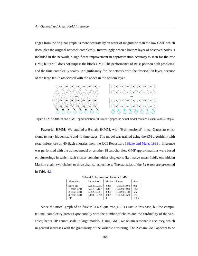
4.4 Generalized Mean Field Inference
edges from the original graph, is more accurate by an order of magnitude than the row GMF, which
decouples the original network completely. Interestingly, when a bottom layer of observed nodes is
included in the network, a significant improvement in approximation accuracy is seen for the row
GMF, but it still does not surpass the block GMF. The performance of BP is poor on both problems,
and the time complexity scales up significantly for the network with the observation layer, because
of the large fan-in associated with the nodes in the bottom layer.
... ...
Figure 4.12: An fHMM and a GMF approximation (illustrative graph; the actual model contains 6 chains and 40 steps).
Factorial HMM: We studied a 6-chain fHMM, with (6-dimensional) linear-Gaussian emis-
sions, ternary hidden state and 40 time steps. The model was trained using the EM algorithm (with
exact inference) on 40 Bach chorales from the UCI Repository[Blake and Merz, 1998]. Inference
was performed with the trained model on another 18 test chorales. GMF approximations were based
on clusterings in which each cluster contains either singletons (i.e., naive mean field), one hidden
Markov chain, two chains, or three chains, respectively. The statistics of theL1 errors are presented
in Table4.3.
Table 4.3:L1 errors on factorial HMM
Algorithm Mean± std Median Range time
naive MF 0.254±0.095 0.269 [0.083,0.397] 9.81-chain GMF 0.237±0.107 0.233 [0.029,0.392] 14.32-chain GMF 0.092±0.081 0.064 [0.019,0.314] 5.63-chain GMF 0.118±0.092 0.089 [0.035,0.357] 15.6BP 0 0 - 106.2
Since the moral graph of an fHMM is a clique tree, BP is exact in this case, but the compu-
tational complexity grows exponentially with the number of chains and the cardinality of the vari-
ables; hence BP cannot scale to large models. Using GMF, we obtain reasonable accuracy, which
in general increases with the granularity of the variable clustering. The 2-chain GMF appears to be
168

4.5 Graph Partition Strategies for GMF Inference
a particularly good granularity of clustering in this case, leading to both better estimation and faster
convergence.
In summary, GMF shows reasonable performance in all three of the canonical models we tested,
and provides a flexible way to trade off accuracy for computation time. It is guaranteed to converge,
and the computational complexity is determined by the treewidth of the subgraph. BP, on the other
hand, may fail to converge. Furthermore, the complexity of computing BP messages is exponential
in the size of the maximal clique in the moralized graph, which makes it very expensive in directed
models with dense local dependencies. However, note that there are multiple ways of decomposing a
graphical model (Fig.4.13); in all three examples just studied, the clusterings of variables are chosen
manually by examining the graph topology and studying the model semantics, and the choice affects
the approximation quality significantly. Can we do this in a more principled way, especially for less
structured graphs? In the following section, we address this problem.
22 y23
y71
y72 y
y74
y75y76
y61
y62 63
y64
y65y66
y51
y52 y53
y54
y55y56
y
y42 y43
y44
y45y46
41
y32 y33
y34
y35
y
21y y24
y25y26
73
y31
y36
y
y11
y12 y13
y14
y15y16
22 y23
y71
y72 y
y74
y75y76
y61
y62 y63
y64
y65y66
y51
y52 y53
y54
y55y56
y
y42 y43
y44
y45y46
41
32 y33
y34
y35
C1
y
21y y24
y25y26
73
y31
y36
y11
y12 y13
y14
y15y16
y
22 y23
y71
y72 y
y74
y75y76
y61
y62 63
y64
y65y66
y51
y52 y53
y54
y55y56
y
y42 y43
y44
y45y46
41
y32 y33
y34
y35
y
21y y24
y25y26
73
y31
y36
y
y11
y12 y13
y14
y15y16
Figure 4.13: Two possible schemes for partitioning a graph to construct the GMF approximation. Which one is better?
4.5 Graph Partition Strategies for GMF Inference
What are the prospects for fully autonomous algorithms for variational inference in graphical mod-
els? Recent years have seen an increasingly systematic treatment of an increasingly flexible range
169

4.5 Graph Partition Strategies for GMF Inference
of algorithms for variational inference. In particular, the cluster variational framework has provided
a range of algorithms that extend the basic “belief propagation” framework[Yedidiaet al., 2001a].
Similarly, general clusters of variables are also allowed in recent treatments of structured mean field
algorithms[Wiegerinck, 2000]. Empirical results have shown that both kinds of generalization can
yield more effective algorithms.
While these developments provide much-needed flexibility for the design of effective algo-
rithms, they also raise a new question—how are the clusters to be chosen? Until now, this issue has
generally been left in the hands of the algorithm designer; moreover, the designer has been provided
with little beyond intuition for making these choices. For some graphical model architectures, there
are only a few natural choices, and these can be explored manually. In general, however, we wish
to envisage a general piece of software for variational inference which can be asked to perform in-
ference for an arbitrary graph. In this setting, it is essential to begin to explore automatic methods
for choosing clusters.
In the previous section, we presented a generalized mean field algorithm for inference based on
adisjointclustering of random variables in a graphical model, noting that the assumption of disjoint
clusters leads to a simple and generic set of inference equations that can be easily implemented.
Disjoint clusters have another virtue as well, which is the subject of this section—they open the
door to a role for graph partitioning algorithms in choosing clusters for inference.
There are several intuitions that support a possible role for graph partitioning algorithms in the
autonomous choice of clusters for graphical model inference. The first is that minimum cuts are to
be preferred, so that as much as possible of the probabilistic dependence is captured within clus-
ters. It also seems likely that the values of parameters should matter because they often reflect the
“coupling strength” of the probabilistic dependences among random variables. Another intuition is
that maximum cuts should be preferred, because in this case the mean field acting across a large cut
may have an expectation that is highly concentrated, a situation which corresponds to the basic as-
sumption underlying mean field methods[Jordanet al., 1999]. Again, specific values of parameters
should matter.
170

4.5 Graph Partition Strategies for GMF Inference
In this section we provide a preliminary formal analysis and a thoroughgoing empirical explo-
ration of these issues. We present a theorem that relates the weight of the graph cut to the quality of
the bound of GMF approximation, and study random graphs and a variety of settings of parameter
values. We compare several different kinds of partitioning algorithms empirically. As we will show,
our results turn out to provide rather clear support for a clustering algorithm based on minimal cut,
which is consistent with implications drawn from the formal analysis. These promising results open
up the possibility for a fully autonomous variational inference algorithm for complex models based
on automatic node partitioning of a graphical model and GMF fixed point iterations as illustrated in
the following flowchart in Figure4.14.
GP GMFq(x )posterior:
approximate jointgraphical model: node clusteringp(x , x )H p(x , x )H EE H
Figure 4.14: Flowchart of a autonomous variational inference algorithm.
4.5.1 Bounds on GMF Approximation
The quality of the GMF approximation depends critically on the choice of variable clustering of the
graphical model. The following is a theorem that formally characterizes this relationship.
Theorem 5 (GMF bound on KL divergence): The Kullback-Leibler divergence from the GMF
approximate joint posterior to the true joint posterior is bounded by the sum of the weights of
potential functions associated with the cross-border cliques, up to some constants intrinsic to the
graphical model:
aW ≤ KL(q‖p) ≤ bW, (4.27)
whereW =∑
Dβ⊆∪Biθβ and,a andb are constants determined by the potential functions of the
cross-border cliques (but independent of the potentials internal to the clusters.)
A proof of this theorem is provided in AppendixB.2. Theorem5 provides a clear guideline
for choosing a desirable partitioning of a general graphical model: heuristically, it is desirable
171
4.5 Graph Partition Strategies for GMF Inference
to break cliques associated with small weights while clustering the variables in the graph; more
systematically, we can use a graph partitioning algorithm to seek an optimal decomposition of the
graph underlying the model. In the following, we explore several graph partitioning strategies on
random graphs with pairwise potentials (each clique contains only two variables) to confirm and
exploit Theorem5 experimentally.
4.5.2 Variable Clustering via Graph Partitioning
A wide variety of graph partitioning algorithms have been explored in recent years in a number of
fields (e.g.,[Goemans and Williamson, 1995; Rendl and Wolkowicz, 1995]). Given our focus on
disjoint clusters in the GMF approach, these algorithms have immediate relevance to the problem
of choosing clusters for inference. In this section, we describe the methods that we have explored.
4.5.2.1 Graph partitioning
Let G(V, E , A) be a weighted undirected graph with node setV = 1, . . . , n, edge setE and
nonnegative weightsaij , for (i, j) ∈ E (aij = 0 if there is no edge between nodei andj; alsoaii =
0,∀i). We refer to the symmetric matrixA = aij as theaffinity matrix. We equip the space ofn×
n matrices with the trace inner productA •B = tr AB; letA 0 denote positive semidefiniteness
(A B denotesA − B 0); and letA ≥ 0 denote elementwise non-negativity ofA. The linear
operator Diag(a) forms a diagonal matrix from the vectora, and its adjoint operator diag(A) yields
a vector containing the diagonal elements ofA. We denote byek the vector containingk ones.
Equi-MinCut. We first consider graph partitioning (GP) problems based on minimum cuts. Given
a graphG(V, E , A) as described above, a classical formulation[Rendl and Wolkowicz, 1995] asks
to partition the node set intok disjoint subsets,(C1, . . . , Ck), of specified sizesm1 ≥ m2 ≥ . . . ≥
mk,∑k
j=1mj = n, so as to minimize the total weight of the edges connecting nodes in distinct
subsets of the partition. This is known as the minimumk-cut of G. In this section, we concern
ourselves with the special case of this problem in which all subsets have equal cardinalitym, a
172

4.5 Graph Partition Strategies for GMF Inference
problem that we refer to ask equi-MinCut(k-MinC). 4 Equi-MinCut avoids potentially skewed
cuts on highly imbalanced graphs, and leads to a balanced distribution of computational complexity
among clusters.
A k-way node partition can be represented by anindicator matrixX ∈ Rn×k with the j-th
column,xj = (x1j x2j . . . xnj)t, being theindicator vectorfor the setCj , ∀j:
xij =
1 : if i ∈ Cj
0 : if i /∈ Cj.
Thus,k-equipartitionsof a graph are in one-to-one correspondence with the set
Fk = X : Xek = en, Xten = mek, xij ∈ 0, 1.
For each partitionX, the total weight of the edges connecting nodes within clusterCi to nodes in
its complementCi is equal to12x
ti(D − A)xi, whereD = Diag(Aen). As a result, the total weight
of thek-cut is
Ck =∑
i
12xt
i(D −A)xi =12
trXtLX, (4.28)
whereL , D −A is theLaplacian matrixassociated withG.
Thus,k equi-MinCut can be modeled as the following integer programming problem
(k-MinC) MinC∗k := mintr XtLX : X ∈ Fk.
Equi-MaxCut. We may also wish to find ak-partition thatmaximizesthe total weight of the cut.
This problem is known as the Maxk-Cut in combinatorial optimization. Even without any size
constraint this problem is NP-hard. In this paper, we again concern ourselves with a constrained
version of the problem, in which all subsets have equal cardinalitym. Thus we have the following
k equi-MaxCut(k-MaxC) problem
(k-MaxC) MaxC∗k := maxtr XtLX : X ∈ Fk
=∑
i
dii −mintr XtAX : X ∈ Fk.
4In combinatorial optimization, this problem is traditionally referred to as thek-partition problem. It is NP-hard, andto be distinguished fromunconstrainedminimum cut, which isnot NP-hard.
173

4.5 Graph Partition Strategies for GMF Inference
We see that bothk-MaxC andk-MinC are quadratic programs, and the relaxations that we con-
sider will treat them identically. Note that due to the equality in the second line of the above equa-
tion, k-MaxC can be solved in a similar manner tok-MinC, which amounts to using a different
“cost” matrix in the objection function.
Weight matrices. The design of the affinity matrix has a fundamental impact on the results that
are produced by graph partition algorithms. The naive choice in our case is to simply letaij = 1
when nodei andj are connected in a graphical model, and letaij = 0 otherwise. Intuitively, an
equi-MinCut using such an affinity matrix will capture more of the local dependency structure in the
model, while an equi-MaxCut will lead to lower computational cost for inference in each cluster.
One can also partition the graphical model based oncoupling strength, i.e., lettingaij = θij ,
the weight of the pairwise potential, so that an equi-MinCut results in clusters with strong intra-
cluster coupling, whereas an equi-MaxCut produces a clustering with only weak couplings left in
each cluster.
It also seems sensible to consider weighting schemes that favor large cuts with small coupling
strength, or small cuts and large coupling strengths. We explore such a scheme by choosing weights
that are inversely related to coupling strength.
The following table summarizes the various partition strategies explored in this paper, and the
corresponding design of the affinity matrix.Table 4.4: Graph partition schemes
GPscheme
k-MinCa
k-MinCb
k-MinCc
k-MaxCa
k-MaxCb
k-MaxCc
aij
value1, 0 θij , 0 1
θij, 0 1, 0 θij , 0 1
θij, 0
4.5.2.2 Semi-definite relaxation of GP
Both k equi-MinCutandk equi-MaxCutare NP-hard. But there exist a variety of heuristics for
finding approximate solutions to these problems[Frieze and Jerrum, 1995; Karisch and Rendl,
1998]. some applicable to quite large graphs[Falkneret al., 1994]. In the sequel, we describe
174
4.5 Graph Partition Strategies for GMF Inference
an algorithm that finds an approximate solution tok-MinC andk-MaxC using a semidefinite
programming (SDP) relaxation[Karisch and Rendl, 1998].
Semidefinite programming. Semidefinite programming (SDP) refers to the problem of optimiz-
ing a convex function over the convex cone of symmetric and positive semidefinite matrices, subject
to linear equality constraints[Vandenberghe and Boyd, 1996]. A canonical (primal) SDP takes the
form:
(SDP)
min C •X
s.t. Ai •X = bi for i = 1, . . . ,mX 0
Because of the convexity of the objective function and the feasible space, every SDP problem has
a single global optimum. With the development of efficient, general-purpose SDP solvers based
on interior-point methods (e.g., SeDuMi[Sturm, 1999]), SDP has become a powerful tool in solv-
ing difficult combinatorial optimization problems. Here, we describe a simple SDP relaxation for
solving graph partitioning problems.
SDP relaxation of GP. We now derive a semidefinite relaxation for GP. For simplicity, we illus-
trate it only fork-MinC; k-MaxC follows similarly with the appropriate change to the objective.
The first step in SDP relaxation involves replacingXtLX with tr LY , whereY is equal to
XXt; this linearizesthe objective. Let us define the setTk:
Tk := Y : ∃X ∈ Fk such thatY = XXt.
Thusk-MinC reads: MinC∗k := mintr LY : Y ∈ conv(Tk).
Note that due to linearization of the objective, our feasible set can be rewritten as the convex hull
of the original setTk. The next step is to approximate the convex hull ofTk by outer approximations
that can be handled efficiently.Karisch and Rendl[1998] describe a nested sequence of outer
approximations for GP that leads from the well-known eigenvalue bound of Donath and Hoffman
to increasingly accurate bounds. Omitting details, one of their relaxation schemes results in the
following SDP relaxation fork-MinC:
175

4.5 Graph Partition Strategies for GMF Inference
(P )
max 12 tr LY
s.t. diag(Y ) = enY en = menY ≥ 0 elementwiseY 0, Y = Y t
(P) is an SDP and can be solved by an interior-point solver such as SeDuMi.
4.5.2.3 Finding a closest feasible solution
While in some cases a bound is the major goal of a relaxation, in our case we require that the
relaxation give us a (feasible) solution. In particular, the optimal solution of problem(P ) is in
general not feasible for the original GP problem, and we need to recover from the approximate
solution a closest feasible solution,X, to the original GP problem. We use the following scheme in
this section.
• From the relaxed solutionY , find a decompositionY = X ′X ′t via SVD (note thatX ′ is usually fullrank rather than of rankk as in the feasible case).
• Treat each row inX ′ as a point inRn; cluster these points using a variant of the standardK-meansalgorithm that finds equi-size clusters. (We use multiple restarts and pick the result with the best cutvalue).
• Complete the feasible index matrixX: xij = 1 iff row i of X ′ gets assigned to clusterj.
This rounding scheme is related to the randomized projection heuristic studied byGoemans and
Williamson[1995] in their work on Max-Cut. In this approach, the label (-1 or +1) of each vector
is chosen according to whether the vector is above or below a randomly chosen hyperplane passing
through the origin.Frieze and Jerrum[1995] generalized this scheme to maxk-cut. Rendl and
Wolkowicz [1995] proposed another alternative involving a first-order Taylor expansion of the cost
function around the relaxedX ′. However, these schemes make it difficult to enforce size constraints
on the clusters, and occasionally produce artifacts such as having an empty cluster. Empirically, we
have found that aK-means heuristic usually leads to superior and often near-optimal results.
176

4.5 Graph Partition Strategies for GMF Inference
4.5.3 Experimental Results
In this section, we combine graph partitioning with the GMF algorithm to perform inference on
randomly generated undirected graphical models with singleton and pairwise potentials. We an-
alyze three aspects of the overall procedure—the quality of the graph partition, the accuracy of
the approximate marginal probabilities, and the tightness of the lower bounds on the log partition
function.
For each trial, we use a random graph of 24 nodes5 and specify the distributionp(x|θ) by
making a random choice of the model parameterθ from a uniform distributionU(a, b). For single
node weightsθi, we seta = −wobs andb = −wobs. For pairwise weightsθij , we seta = −wcoup,
b = 0 for repulsivecoupling;a = −wcoup, b = wcoup for mixedcoupling; anda = 0, b = wcoup for
attractivecoupling, respectively.
Table 4.5: GP performance. (default:K-means rounding; rp: random projection rounding)Equi-MinCut Equi-MaxCut
k lower-b feas.X f/b upper-b feas.X f/b feas.X (rp) f/b (rp)3 34 38 1.10±0.03 78 75 0.96±0.02 71 0.91±0.044 41 45 1.09±0.02 82 80 0.97±0.02 74 0.90±0.046 52 55 1.06±0.03 83 81 0.97±0.01 77 0.93±0.028 59 61 1.03±0.02 83 82 0.99±0.01 79 0.95±0.02
3 73 77 1.05±0.02 122 119 0.97±0.01 113 0.92±0.034 86 90 1.05±0.02 135 130 0.97±0.01 122 0.91±0.036 104 207 1.03±0.01 140 137 0.98±0.01 128 0.91±0.028 116 118 1.02±0.01 140 138 0.99±0.01 131 0.93±0.01
4.5.3.1 Partitioning random graphs
Our graphs are generated by sampling an edge with probabilityp for each pair of nodes. Table4.5
summarizes the performance (over 100 trials) of various graph partition schemes on random graphs.
To assess performance, we compute the ratiof/b between the feasible cut that was found and the
bound on the optimal cut provided by the SDP relaxation (the optimal solution must fall between
f andb). In the top panel, we show results for partitioning unweighted graphs withp = 0.3 into
5In fact, a standard SDP solver can readily handle larger graphs (e.g., with more than 100 nodes). But the exactsolutions of the singleton marginals for larger graphs are very expensive to compute, which makes it difficult to obtaingood estimates of the inference error.
177
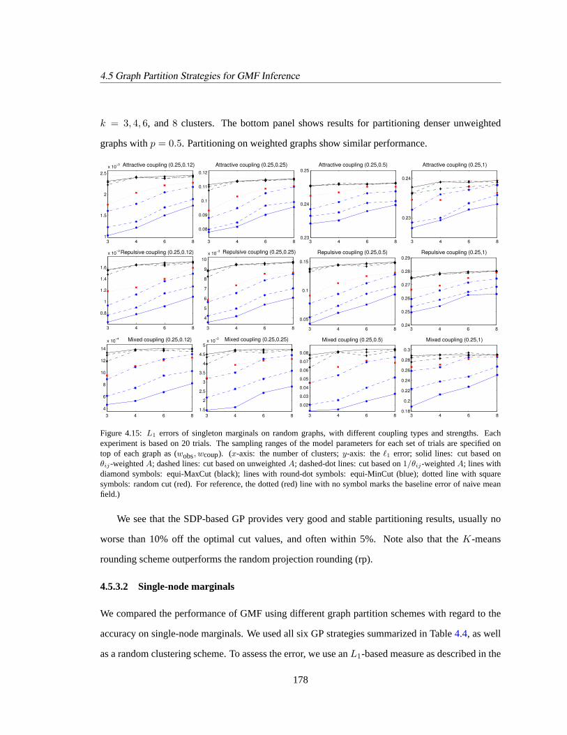
4.5 Graph Partition Strategies for GMF Inference
k = 3, 4, 6, and8 clusters. The bottom panel shows results for partitioning denser unweighted
graphs withp = 0.5. Partitioning on weighted graphs show similar performance.
3 4 6 8
0.8
1
1.2
1.4
1.6
x 10−3 Repulsive coupling (0.25,0.12)
3 4 6 8
0.08
0.09
0.1
0.11
0.12
Attractive coupling (0.25,0.25)
3 4 6 80.23
0.24
0.25Attractive coupling (0.25,0.5)
3 4 6 8
0.23
0.24
Attractive coupling (0.25,1)
3 4 6 81
1.5
2
2.5x 10⁻³ Attractive coupling (0.25,0.12)
3 4 6 80.24
0.25
0.26
0.27
0.28
0.29Repulsive coupling (0.25,1)
3 4 6 84
6
8
10
12
14
x 10−4 Mixed coupling (0.25,0.12)
3 4 6 81.5
2
2.5
3
3.5
4
4.5
5x 10⁻³ Mixed coupling (0.25,0.25)
3 4 6 8
0.05
0.1
0.15
Repulsive coupling (0.25,0.5)
3 4 6 8
0.02
0.03
0.04
0.05
0.06
0.07
0.08
Mixed coupling (0.25,0.5)
3 4 6 80.18
0.2
0.22
0.24
0.26
0.28
0.3
Mixed coupling (0.25,1)
3 4 6 8
4
5
6
7
8
9
10x 10−3 Repulsive coupling (0.25,0.25)
Figure 4.15:L1 errors of singleton marginals on random graphs, with different coupling types and strengths. Eachexperiment is based on 20 trials. The sampling ranges of the model parameters for each set of trials are specified ontop of each graph as (wobs, wcoup). (x-axis: the number of clusters;y-axis: the`1 error; solid lines: cut based onθij-weightedA; dashed lines: cut based on unweightedA; dashed-dot lines: cut based on1/θij-weightedA; lines withdiamond symbols: equi-MaxCut (black); lines with round-dot symbols: equi-MinCut (blue); dotted line with squaresymbols: random cut (red). For reference, the dotted (red) line with no symbol marks the baseline error of naive meanfield.)
We see that the SDP-based GP provides very good and stable partitioning results, usually no
worse than 10% off the optimal cut values, and often within 5%. Note also that theK-means
rounding scheme outperforms the random projection rounding (rp).
4.5.3.2 Single-node marginals
We compared the performance of GMF using different graph partition schemes with regard to the
accuracy on single-node marginals. We used all six GP strategies summarized in Table4.4, as well
as a random clustering scheme. To assess the error, we use anL1-based measure as described in the
178

4.5 Graph Partition Strategies for GMF Inference
last section. The exact marginals are obtained via exhaustive enumeration. We used graphs of two
different densities in our experiments:moderately connectedgraphs, with treewidth12 ± 1, more
than an order of magnitude greater than the largest cluster to be formed; anddensely connected
graphs, with treewidth16 ± 1. For simplicity, we show only results for the moderately connected
graphs.
Figure4.15shows that for all variable clusterings, GMF almost always improves over the naive
mean field. As expected, equi-MinCut always provides better results than other partition strate-
gies. In particular, equi-MinCut based on coupling strength yields the best results (consistent with
Theorem 5), followed by equi-MinCut based on node degree, then equi-MinCut that cuts the least
number of heavy edges. This suggests that, to better approximate the true marginals, it is important
to capture strong couplings within clusters. Equi-MaxCut fares less well; indeed, it is worse than
a random cut in most cases. It is worth noting, however, that cutting lightweight edges (i.e., max-
imizing the sum of 1θij
across clusters) leads to better performance than degree- or coupling-based
cuts.
Not surprisingly, the performance of GMF improves as the size of the clusters increase, which
allows more dependencies to be captured within each cluster.
For denser graphs (results not shown), the performance gap between different clustering schemes
becomes smaller, but the trend and the relative order remain the same.
4.5.3.3 Bounds on the log partition function
Figure4.16shows the lower bounds on the log partition functions given by the GMF approxima-
tions. Comparing to Figure4.15, we see that there is a good correspondence between the perfor-
mance on approximating marginals and the tightness of the lower bound, a reassuring result in the
context of mean-field algorithms.
In summary, our empirical results provide rather clear support for a weighted version of MinCut
as a useful clustering algorithm for GMF inference, which is consistent with the implications from
179

4.5 Graph Partition Strategies for GMF Inference
3 4 6 80.988
0.99
0.992
0.994
0.996
0.998Attractive coupling (0.25,0.12)
3 4 6 80.955
0.96
0.965
0.97
0.975
0.98
0.985Attractive coupling (0.25,0.25)
3 4 6 8
0.974
0.976
0.978
0.98
0.982Attractive coupling (0.25,0.5)
3 4 6 80.98
0.982
0.984
0.986
0.988
0.99Attractive coupling (0.25,1)
3 4 6 80.99
0.992
0.994
0.996
0.998Repulsive coupling (0.25,0.12)
3 4 6 80.96
0.965
0.97
0.975
0.98
0.985
0.99Repulsive coupling (0.25,0.25)
3 4 6 80.94
0.945
0.95
0.955
0.96
Repulsive coupling (0.25,1)
3 4 6 80.992
0.994
0.996
0.998
1Mixed coupling (0.25,0.12)
3 4 6 80.975
0.98
0.985
0.99
0.995Mixed coupling (0.25,0.25)
3 4 6 80.9
0.93
0.96Mixed coupling (0.25,1)
3 4 6 80.88
0.9
0.92
0.94
0.96
Repulsive coupling (0.25,0.5)
3 4 6 8
0.92
0.94
0.96
0.98Mixed coupling (0.25,0.5)
Figure 4.16: Accuracy of the lower bound on the log partition function. The ordering of the panels and the legends are thesame as in Fig4.15, except that they-axis now corresponds to the ratio of the lower bound of the log partition functiondue to GMF versus the true log partition function.
180

4.6 Extensions of GMF
the formal analysis. This combination of graph partitioning algorithms with the generalized mean
field inference algorithm manifests a promising prototype for an autonomous variational inference
algorithm for arbitrary graphical models, optimizing variational approximations over the space of
model parameters as well as over the choice of tractable families used for the variational approxi-
mation, and making it possible to perform distributed approximate inference on large-scale network
models arising from challenging problems in fields such as systems biology and sensor networks.
4.6 Extensions of GMF
In light of the foregoing exposition, there are a number of extensions of the research reported here
that potentially lead to further improved GMF approximation.
4.6.1 Higher Order Mean Field Approximation
One possible extension involves the use of higher-order expansions in the basic variational bounds.
Leisink and Kappen[2001] have shown how to upgrade first-order variational bounds such as that
shown in Eq. (4.7) to yield higher-order bounds. In particular, the following third-order lower bound
can be obtained for the likelihood:
p(xE) ≥∫dx exp
− E′(xH)
[1−∆ +
12
exp(ξ)∆2],
whereξ = 13〈∆
3〉/〈∆2〉, ∆ = E(xH ,xE)− E′(xH), and〈·〉 denotes expectation over the approx-
imate distributionq(xH) = exp−E′(xH). The optimizer of this lower bound cannot be found
analytically. However, we can compute the gradient of the lower bound with respect toE′i (assuming
a cluster-factorized approximate distribution), which requires computation of up to third-order cu-
mulants of the nodes in the bordering cliques in the subgraph.Leisink and Kappen[2001] reported
an application of such a strategy to the 2-D lattice model and sigmoid belief network, approximated
by a completely disconnected subgraph, and reported significantly improved bounds. In the GMF
setting, which uses an approximating subgraph with more structure, the computation of the gradient
is even simpler because fewer nodes are involved in the cumulant calculation.
181

4.6 Extensions of GMF
4.6.2 Alternative Tractable Subgraphs
Another possible extension is to replace the disjoint clustering with atree-connected clustering.
The termW in the GMF bound can be also viewed as the total weight of the disrupted cliques (with
respect to the original graph) in the subgraph underlying a GMF approximation. Thus, we may
further reduceW by departing from the completely disjoint clustering to tree-connected clusters,
in which we connect all the disjoint clusters resulting from a graph partition using a tree whose
nodes are clusters. The link between every pair of connected clusters is chosen to be the maxi-
mally weighted clique shared by the clusters. Such a tree can be easily obtained by constructing a
maximal spanning tree of variable clusters. The motivation of using tree-connected clusters rather
than arbitrary subgraphs to approximate the true joint distribution is that under such a subgraph, the
message-passing-based GMF algorithm described earlier is still guaranteed to converge and yield a
set of globally consistent approximate cluster marginals.
4.6.3 Alternative Graph Partitioning Schemes
Eq. (B.5) in the appendix suggests that it may be advantageous to use other weighting schemes,
such as the entropy-like clique weights (expected potentials)〈φβ〉q, and seek a partition that min-
imizes the sum of expected cross-border potentials. Obviously, exact computation of the entropy-
like weights requires the true joint distribution, and is thus infeasible. We may approximate the
expected potential of each clique by replacing the true marginal distribution of the variables in
the corresponding clique with a naive mean-field-like approximation to the marginal:q(xDβ) ∝
expθβφβ(xDβ)|Fβ whereF denotes mean field messages from neighboring cliques; this turns
the computation of the expectation into a local computation. It is possible to use an algorithm that
iterates between GMF (to update the marginalq(·)) and GP (to update the partition). It would be
also interesting to look at unequal partitions in MinCut, which allows modularities of the graph
structure to be explored in a more flexible way (e.g., as we do in the following for theLOGOS
model).
182

4.7 Application to the LOGOS Model
4.7 Application to the LOGOS Model
The generalized mean field theorem makes it straightforward to obtain the fixed-point equations
of the variational approximation to a variety of probability distributions of practical interest. All
that is needed is to decide on a subgraph and a variable clustering, to identify the Markov blanket
of each cluster, and to plug in the mean fields of the Markov blanket variables according to Eqs.
(4.23) (or more generally, the marginal potentials of the peripheral cliques of each cluster). As
pointed out in Remark 1, since all the original intra-cluster dependencies are preserved in the mean
field cluster marginal, probabilistic inference in the GMF approximate distribution is reduced to
local and modular operations within each cluster. Hence, the overall inference problem is fully
decomposed based on the variable clustering.
Figure 4.17: The modular structure of theLOGOS motif model.
For theLOGOS model developed in Chapter 2 forN sequences containingK types of mo-
tifs, the modularity of the model structure naturally suggests a bipartite variable clustering: amo-
tif cluster S(k)
l , θ(k)
l | k = 1, . . . ,K, l = 1, . . . , Lk, and asequence clusterY (n)
t , X (n)
t | n =
1, . . . , N, t = 1, . . . , Tn (Fig. 4.17). Applying Corollary3, we obtain the following GMF cluster
marginals:
qs(x) ∝N∏
n=1
p(x(n)|υ,Υ)p(y(n)|x(n), 〈ln θ(k)〉qmK
k=1, θbg), (4.29)
qm(θ, s) =K∏
k=1
p(s(k)|ν,Ω)p(θ(k)|s(k), α, 〈h(k)(x,y)〉qsK
k=1) (4.30)
183

4.7 Application to the LOGOS Model
where〈h(k)(x,y)〉qs
is the expectation of the sufficient statistics for motifk determined from DNA
sequence sety by state sequencesx (i.e., the count matrix of nucleotides of all sequence sites that are
of motif k as specified byx); and〈ln θ(k)〉qm
is the posterior means of the logarithms of the position-
specific multinomial parameters of the motifk (often referred to as the natural parameters of the
multinomial distribution). Note thatqs(x) is now just a re-parameterized HMM, andqm(θ, s) is a
re-parameterized HMDM model. Inference in both submodels is straightforward and inexpensive.
For simplicity, again we omit the super(sub)scriptsk andn in the following expositions, and give
equations for a generic motif type or a generic sequence.
4.7.1 A GMF Algorithm for Bayesian Inference in LOGOS
Due to the isomorphism of GMF approximations of the cluster marginals to the original local and
global submodels ofLOGOS (Eqs. (4.29∼4.30)), variational Bayesian inference onLOGOS can
be “divided and conquered” into coupled local inferences on: 1) the isolated local alignment model,
i.e., an HMDM, as if we had “observations”,h = 〈h(x,y)〉qs
, to obtain the posterior distribu-
tion of the PWM of each motif; and 2) the isolated global distribution model, i.e., an HMM,
as if the position-specific multinomial parameters of the motifs, in the natural parameter form
φ(θ) = 〈ln θ〉qm
were given, to compute the posterior probabilities of motif locations. This gives
rise to the following EM-like fixed-point iteration procedure (referred to as a “variational EM” al-
gorithm in[Ghahramani and Beal, 2001], although strictly speaking the analogy is only procedural
but not mathematical, because GMF is not doing maximal likelihood parameter estimation as in an
EM algorithm but Bayesian estimation.), which is a special case of the GMF algorithm in§4.4.3:
Variational “E” step : Compute the expected sufficient statistics, the count matrixh, via inference
in the global motif distribution model givenφ(θ) and sequencey:
h =T−L+1∑
t=1
h(yt:t+L−1)p(Xt = 1|y, φ), (4.31)
wherep(Xt = 1|y) is the posterior probability of the indicator at positiont being the motif-
start state, which can be computed using the forward-backward algorithm. (See AppendixA.3
184

4.7 Application to the LOGOS Model
for details.)
Variational “M” step : Compute the posterior mean of the natural parameter,φ(θ), via inference
in the local motif alignment model givenh:
φ(θl,j) =∫
θ
∑sl
ln θl,jp(θl|sl, α, h)p(sl|h)dθl
=I∑
i=1
p(Sl = i|h)(Ψ(αi,j + hl,j)−Ψ(|αi|+ |hl|)
), (4.32)
whereΨ(x) is the digamma function, andp(Sl = i|h) is the posterior probability of hidden
stateq given ’observation’h, which can be computed using the standard forward-backward
algorithm of HMM. (See AppendixA.4 for details.)
According to Theorem4, this message-passing procedure will converge. Once it converges, we
can compute the MAP estimate of motif locations in the global HMM submodel and the Bayesian
estimate of the motif PWMs from the local HMDM submodels.
The generalized mean field theory provides adivide-and-conquercomputational tool to work
with complex models, especially for those coming from a modular design using the graphical model
formalism. It provides computational support for an upgrade path toward more sophisticated mod-
els, which may be needed for improving motif detection. For example, the global distribution model
is completely open to user design and can be made highly sophisticated to model complex properties
of multiple motifs without complicating the inference in the local alignment model. Similarly, the
local motif alignment model can also be more expressive without interfering with the motif distri-
bution model. In the literature, Bayesian inference in large scale models are usually approached via
a Monte Carlo sampling algorithm. In Chapter 5 we describe acollapsedGibbs sampling procedure
for Bayesian inference onLOGOS. Following is an illustration of the convergence behavior of the
GMF algorithm onLOGOS and an empirical comparison of the GMF algorithm and the Gibbs
sampling algorithm onLOGOS for motif detection tasks of modest difficulty.
185

4.7 Application to the LOGOS Model
4.7.2 Experimental Results
We use semi-realistic test datasets described before, each containing 20 artificially generated DNA
sequences (500-600 bp long) harboring one real motif or three different real motifs (of length 18,
22, and 26 bases, respectively). The performance of inference is evaluated based on the error rate
((false positive + false negative)/2) of predicted motif occurrences.
4.7.2.1 Convergence behavior of GMF
Since the GMF algorithm is only guaranteed to convergence to a local minimum, we run GMF
with 50 random restarts, each followed by fixed-point (FP) iterations until convergence. To obtain
a “convergence curve” of a full run of multiply restarted GMF, we sequentialize the output of all
rounds of FP iterations. After each single cross-update step in each single round of FP-iteration, we
record the lowest value of the free energy,〈E〉q + Hq, achieved so far (since the first round of FP
iteration), and compute the empirical error rates of motif prediction made from the GMF posterior
q corresponding to the current lowest free energy, which gives a performance trace.
0 2 4 6
x 104
−1600
−1400
−1200
−1000
−800
CPU time
− (fr
ee e
nerg
y)
Convergence of GVIGMF
0 20 40 60−2000
−1750
−1500
−1250
−1000
−750
FP−iteration step
− (fr
ee e
nerg
y)
Convergence of FP−iteration
(a) (b)
Figure 4.18: (a) Convergence of a single round of FP-iteration of GMF (Each point represents one step of iteration.) (b)The “convergence curve” of GMF with 50 random re-starts. (The solid line is the mean value over 10 independent runs,and the dashed line represents the std.)
Figure4.18illustrates the convergence behavior of GMF on a motif detection task. Typically,
a single round of GMF takes about30 ∼ 60 iterations to converge (Fig4.18a). GMF with multiple
random restarts in general plateaus within less then 50 restarts (Fig4.18b), suggesting a possibility
186

4.7 Application to the LOGOS Model
of reaching global (or near global) optimality. Thus, in the following experiments, we perform GMF
with 50 random restarts and pick the one resulting in the lowest free energy for the given sequences
as the final result.
4.7.2.2 A comparison of GMF and the Gibbs sampler for motif inference
We compared the performance of motif inference on theLOGOS model using GMF and a Gibbs
sampler (see§5.2). Convergence of the Gibbs sampler is diagnosed based on the standard Gelman-
Rubin (GR) statistics[Gelman, 1998]. We infer motif locations using the sample means ofX during
Gibbs sampling, which yield an on-line measure of the performance.
Table 4.6: Median hit-rate of motif detection in test set containing one genuine and one decoy motif.abf1 gal4 gcn4 gcr1 mat mcb mig1 crp
GMF 0.81 0.82 0.71 0.65 0 0. 0.73 0.58Gibbs 0.71 0.79 0.65 0.53 0.75 0 0.91 0.63
Table4.6summarizes the results obtained via GMF and Gibbs sampling for motif detection in
a simple one-per-sequence setting using HMDM as the local model (see§2.4.4). The performances
of the two algorithms are largely comparable, with the Gibbs sampler slightly better. However, the
convergence time for the Gibbs sampler is significantly longer, typically 5 to 10 times that of GMF.
0 2 4 6
x 104
0
0.2
0.4
0.6
0.8
1
CPU time
erro
r rat
e
Performance of GSVIGMF
0 1 2 3 4
x 105
0
0.2
0.4
0.6
0.8
1
CPU time
erro
r rat
e
Performance of Gibbs sampler
(a) (b)
Figure 4.19: Comparison of GMF and Gibbs sampler on performance (in terms of predictive error rate vs. time). Notethe difference in the scale of the x-axis in the two plots.
For more difficult problems, such as simultaneous detection of multiple motifs in a large dataset,
the mixing time of the Gibbs sampler becomes prohibitively long, and the results obtained within
187

4.8 Conclusions and Discussions
a tolerable time span from a Gibbs sampler are not comparable to those of the GMF, which uses
far less time. Figure4.19illustrates the convergence curve, in terms of predictive error rate versus
time, for GMF and the Gibbs sampler (obtained from the same experiment from which we plotted
the convergence curve in Fig.4.18). As evident in Fig4.19a, the error rate of motif detection using
GMF generally follows an improving trend consistent with that of the free energy in Fig.4.18b,
although not exactly monotonically decreasing, which is not surprising since the generative model
described byLOGOS does not necessarily model the motif sequences exactly (thus some local
optima may yield slightly better predictions than others). The error curve of the Gibbs sampler,
on the other hand, is less stable (Fig4.19b), showing that the sampling process explores the state
space in a non-deterministic fashion, therefore providing less reliable performance in finite time.
The choice of random seeds seems to affect convergence quality for both GMF and Gibbs.
Table 4.7: Performance (mean error rate) of GMF and Gibbs over 5 test datasets.dataset 1 2 3 4 5GMF 0.27±0.17 0.26±0.13 0.38±0.18 0.35±0.18 0.39±0.17Gibbs 0.49±0.19 0.41±0.23 0.56±0.20 0.41±0.23 0.49±0.21
Table4.7summarizes the the performances of GMF and the Gibbs sampler over 5 different test
datasets for simultaneous detection of three motifs (as described in§2.6.1). GMF outperforms the
Gibbs sampler (run with finite allowable time, i.e.10× the time for GMF) in all cases. We reason
that for a complex motif model such asLOGOS, the state space is likely to be highly multi-modal
and poorly connected, and thus tends to trap the Gibbs sampler at sub-optimality; whereas GMF can
explore such a space much more efficiently by doing more random restarts than a Gibbs sampler
can afford, and is guaranteed to reach a local minimum from each restart.
4.8 Conclusions and Discussions
We have presented a generalized mean field approach to probabilistic inference in graphical models,
in which a complex probability distribution is approximated via a distribution that factorizes over
a disjoint partition of the graph. Locally optimal variational approximations are obtained via an
algorithm that performs coordinate ascent on a lower bound of the log-likelihood, with guaranteed
188
4.8 Conclusions and Discussions
convergence. For a broad family of models in practical use, we showed that the GMF approxima-
tions of the cluster marginals are isomorphic to the original model in the sense that they inherit all
of its intra-cluster independence structure. Moreover, these marginals are independent of the rest of
the model given the expected potential factors (mean fields) of the Markov blanket of the cluster.
The explicit and generic formulation of the “mean fields” in terms of the Markov blanket of vari-
able clusters also leads to a simple, generic message-passing algorithm for complex models. This
result is somewhat surprising as it shows that we can do approximate inference for arbitrary subsets
of hidden variables locally and tractably by capturing all the dependences external to the variable
subset with an expected Markov blanket, and applying existing inference algorithms locally (i.e., on
the cluster marginal) as a subroutine.
Disjoint clusterings have also been used in sampling algorithms to improve mixing rates for
large problems. For example, the Swendsen-Wang algorithm[1987] samples the Ising (or Potts)
model at critical temperatures by grouping neighboring nodes with the same spin value, thereby
forming random clusters (of coupled spins) that are effectively independent of each other, allowing
an MCMC process to collectively sample the spin of each cluster independently and at random. This
method often dramatically speeds up the mixing of the MCMC chain.[Gilks et al., 1996] also noted
that when variables are highly correlated in the stationary distribution, blocking highly correlated
components into higher-dimensional components may improve mixing. However, in the sampling
framework, clusterings are usually obtained dynamically, based on the coupling strength rather than
the topology of the network.
We have also investigated combinations of graph partitioning algorithms with the generalized
mean field algorithm, which allows mean field approximations to be optimized over both parameter
space and variable partition space in an autonomous fashion. We proved that the quality of the GMF
approximation is bounded by the total absolute weight of the potentials of the disrupted cliques due
to the disjoint variable clustering. Empirically, we confirmed that although all graphs partitions
lead to improvement over a naive mean field approximation, a minimal cut equipartition clearly
yields the best GMF approximation, measured both by singleton marginals and lower bounds of
189

4.8 Conclusions and Discussions
the true log partition function. Moreover, there is a good association between the qualities of the
approximate marginals and lower bounds.
Our work represents an initial foray into the problem of choosing clusters for cluster-based
variational methods. There is clearly much more to explore. First, we should note that we are
far from the ideal approach, where we base the clustering criterion on the ultimate goal—that of
obtaining accurate estimates of marginal probabilities. This is of course an ambitious goal to aim for,
and in the near term it seems advisable to attempt to find effective surrogates. In particular, we do not
want the problem of choosing clusters to be as computationally complex as the inference problem
that we wish to solve! (Fortunately, many efficient solvers are available to solve the GP problem
nearly optimally via SDP or spectral relaxation.) We should consider surrogates that involve more
general combinations of parameter values along cuts. In particular, we found little support for the
use of maximum cuts in our experiments, but perhaps if we search for large cuts along which the
parameter values are uniformly small we will have more success in this regard. In general, we might
ask for a surrogate that aims to capture both the setting under which mean field approximations are
effective, and the setting under which important local dependencies can be treated tractably.
Note also that we have focused on partitioning methods that decompose a large graphical model
into clusters of equal size. With no prior knowledge of the local connectivity within the clusters,
this equal-size heuristic seems reasonable; we wish to distribute resources roughly equally to each
cluster (e.g., to balance the load in a parallel computing setting). Again, however, it would be useful
to explore surrogates that attempt to capture local connectivity in the clustering criterion.
In an exemplary biological motif detection problem involving Bayesian inference in a hybrid,
large-scale graphical model, GMF outperforms conventional Gibbs sampling methods in both con-
vergence speed and error rate. We believe that due to its flexibility and efficiency, GMF simplifies
the application of variational methods to general probabilistic inference, and can significantly in-
crease the expressive power of languages that can be considered “practical” for knowledge repre-
sentation and reasoning under uncertainty.
190

Chapter 5
Probabilistic Inference II: Monte CarloAlgorithms
Monte Carlo algorithms are based on the fact that while it may not be feasible to perform statis-
tical computations on a complex joint or posterior distribution, say,p(x), it may be possible to
obtain samples fromp(x), or from a closely related distribution, such that marginals and other
expectations can be approximated using sample-based averages. In contrast to the variational in-
ference approaches discussion in the previous chapter, which seek deterministic approximations to
p(x), Monte Carlo algorithms yield a stochastic representation ofp(x) that is asymptotically ex-
act and easy to apply. General-purpose Monte Carlo inference software such as the BUGS system
has been developed for use with a general-purpose statistical modeling language (see[Gilks et al.,
1996]). For some statistical models, such as the Dirichlet process mixture model for haplotypes and
non-parametric Bayesian models in general, although the variational approach has been vigorously
pursued[Blei and Jordan, 2004], so far Monte Carlo algorithms are still the only practical approach
to yield reliable performance.
5.1 A Brief Overview of Monte Carlo Methods
We discuss two examples of Monte Carlo algorithms—Gibbs sampling and the Metropolis-Hastings
algorithm—that are commonly used in the graphical model setting and in particular within the
Bayesian paradigm.
191
5.1 A Brief Overview of Monte Carlo Methods
Gibbs sampling is an example of a Markov chain Monte Carlo (MCMC) algorithm. In an
MCMC algorithm, samples are obtained via a Markov chain whose stationary distribution is the
desiredp(x) (typically a complex multivariate distribution). The state of the Markov chain is an
assignment of a value to each of the variables. After a suitable “burn-in” period so that the chain
approaches its stationary distribution, these states are used as samples.
The Markov chain for the Gibbs sampler is constructed in the following way: 1) at each step
one of the variablesXi is selected (at random or according to some fixed sequence); 2) the condi-
tional distributionp(xi|xV\i) is computed (recall thatV is the set of indices of all the variables in
a graphical modelG(V, E)); 3), a valuexi is sampled from this distribution; and 4) the sampledxi
replaces the previous value of theith variable.
The Markov properties of graphical models are particularly useful for a Gibbs sampler: condi-
tioning on the so-called Markov blanket of a given node renders the node independent of all other
variables. Therefore,p(xi|xV\i) = p(xi|xMBi). Thus, the implementation of Gibbs sampling re-
duces to the computation of the conditional distributions of individual variables given their Markov
blankets. For graphical models, these conditionals take the following form:
p(xi|xV\i) = p(xi|xMBi)
=
∏α∈MBKi
φα(xDα)∑xi
∏α∈MBKi
φα(xDα)(5.1)
whereMBKi denotes the set of cliques containingXi and its Markov blanket nodes (note the
difference ofMBKi andMBCi defined in Chapter 4). The setMBKi is often much smaller than
the setD of all cliques ofG, and in such cases each step of the Gibbs sampler can be implemented
efficiently. Indeed the computation of the conditionals often takes the form of a simple message-
passing algorithm that is reminiscent of the junction tree algorithm or the GMF algorithm.
When the computation in Eq. (5.1) is overly complex, the Metropolis-Hastings algorithm can
provide an effective alternative. Metropolis-Hastings is an MCMC algorithm that is not based on
conditional probabilities, and thus does not require normalization as in Eq. (5.1). Given the current
statex of the algorithm, Metropolis-Hastings chooses a new statex∗ from a “proposal distribution”
192

5.2 A Gibbs Sampling Algorithm for LOGOS
q(x∗|x), which often simply involves picking a variableXi at random and choosing a new value for
that variable, again at random. The algorithm then computes the “acceptance probability”:
ξ = min(
1,q(x|x∗)q(x∗|x)
∏α∈A φα(x∗Dα
)∏α∈A φα(xDα)
). (5.2)
With probabilityξ the algorithm accepts the proposal and moves tox∗, and with probability1 − ξ
the algorithm remains in statex. For graphical models, if only one of the variables (sayXi) is
resampled, this computation also turns out to often take the form of a simple message-passing
algorithm, of which samples of the Markov blanket ofXi can be regarded as themessage.
The principal advantages of Monte Carlo algorithms are their simplicity of implementation and
their generality. Under weak conditions, the algorithms are guaranteed to converge. A problem with
the Monte Carlo approach, however, is that convergence times can be long (e.g., see§4.7.2), and it
can be difficult to diagnose convergence.
5.2 A Gibbs Sampling Algorithm for LOGOS
In the last chapter, we described a GMF algorithm for variational Bayesian inference forde novo
motif detection under theLOGOS model, which deterministically approximates the posterior distri-
bution of motif locations and the Bayesian estimates (resulted from an integration over the posterior
distribution) of PWMs. Here we present a Gibbs sampling algorithm for the same tasks. A compar-
ison of its performance to that of the GMF algorithm was given in§4.7.2.
5.2.1 TheCollapsedGibbs Sampler
Given a set of DNA sequences denoted byy = y(n)Nn=1, wherey(n) = (y(n)
1 , . . . , y(n)Tn
), a
Gibbs sampler periodically samples the state configurations of latent variables from variable sets
X = X(n)Nn=1, Θ = θ(k)K
k=1 andS = S(k)Kk=1, one at a time, conditioning on the state
configurations of the rest of the variables sampled during the previous iterations. Again, for sim-
plicity we drop in the sequel the superscriptn associated with variablesX,Y , and the superscript
k associated with variablesθ, S. The predictive distributions to be derived for sampling apply to
every sequence and motif.
193

5.2 A Gibbs Sampling Algorithm for LOGOS
In principal, a standard data augmentation (DA)[Tanner and Wong, 1987] approach can be
used to solve the Bayesian missing data problem for motif detection underLOGOS. But the fact
thatθ is a high-dimensional continuous variable implies that it is very expensive to approximate its
posterior distribution by samples and also, the Markov chain that generates these samples can mix
very slowly. As pointed out inLiu [1994], the conjugacy betweenp(θ, s) andp(x,y|θ) suggests
that we can integrate outθ and derive acollapsedGibbs sampling scheme. Essentially, we sample
iteratively from only two sets of discrete variables in the Markov chain: the Dirichlet component
indicator sequenceS = (S1, . . . , SL) in the local HMDM model, and the motif location indicator
sequenceX = (X1, . . . , XT ) in the global HMM model.
Let l denote an arbitrary state taken byXt (i.e, columnl of a motif whose index is omitted)
and, andh denote the sufficient statistics of the PWMθ (i.e., the nucleotide count matrix of the
aligned instances of each motif). For convenience, we use the subscript[−t] to denote an index set
excluding thetth element for variables, or an indication of the source (i.e., all but thetth element)
from which a sufficient statistic is collected. To keep the exposition simple, in the sequel we focus
on a Bayesian treatment of the PWMs only, and let the transition probability matricesΩi,j and
Υi,j in the global and local model, respectively, be constant. A Bayesian treatment of these
parameters (e.g.,Ω) was discussed in§3.2, and can be similarly implemented in the collapsed Gibbs
sampler. Given the current states of all (discrete) variables in theLOGOS model exceptXt, the
Bayesian conditional predictive distribution forXt is:
p(Xt = l|x[−t], s,y)
= p(Xt = l|xt−1, xt+1, yt, h[−t], s)
=1Zp(Xt = l|xt−1, xt+1)p(yt|Xt = l, h[−t], sl)
=1Z
Υxt−1→lΥl→xt+1
Γ(|αsl|)∏
j∈N Γ(αsl,j)
∫ ∏j∈N
θαsl,j
+h[−t],l,j+δ(yt,j)−1
j dθj
=1Z
Υxt−1→lΥl→xt+1
Γ(|αsl|)∏
j∈N Γ(αsl,j)·∏
j∈N Γ(αsl,j + h[−t],l,j + δ(yt, j))Γ(|αsl
+ h[−t],l + 1|)
=1Z
Υxt−1→lΥl→xt+1
Γ(|αsl|)∏
j∈N Γ(αsl,j)·∏
j∈N Γ(αsl,j + hl,j)Γ(|αsl
+ hl|), (5.3)
194

5.2 A Gibbs Sampling Algorithm for LOGOS
wherehl represents the count vector of columnl of a motif (whose index is omitted) resulting
from the current assignment ofx[−t] plus the count induced byxt, andΥα→β denotes the transition
probability from stateα to β.
Given the current states of all variables exceptSl, the Bayesian conditional predictive distribu-
tion of variableSl is:
p(Sl = i|s[−l],x,y) = p(Sl = i|sl−1, sl+1, hl)
=1Zp(Sl = i|sl−1, sl+1)p(hl|sl = i)
=1Z
Ωsl−1→iΩi→sl+1
Γ(|αi|)∏j∈N Γ(αi,j)
∫ ∏j∈N
θαi,j+hl,j−1j dθj
=1Z
Ωsl−1→iΩi→sl+1
Γ(|αi|)∏j∈N Γ(αi,j)
·∏
j∈N Γ(αi,j + hl,j)Γ(|αi + hl|)
(5.4)
A full sweep of variablesXn results in a new set of labellings of motif/background in a DNA se-
quence and requiresO(TKL) operations. The maximala posterioriestimates of the motif locations
are obtained by summarizing the empirical sample statistics.
5.2.2 Convergence Diagnosis
Since motifs are short stochastic substring patterns in a large “sea” of background sequences, the
posterior distribution defined byLOGOS is not only very high-dimensional, but also likely to be
multi-modal due to the possible presence of many genuine or pseudo motif patterns in the sequences.
Such a distribution can cause very slow mixing for the Markov chain, as well difficulties in detecting
when the stationary distribution is reached.
0 1000 20001
1.5
2chain 1
0 1000 20001
1.5
2chain 2
0 1000 20001
1.5
2chain 3
0 1000 20001
1.5
2chain 4
0 1000 20001
1.5
2chain 5
Figure 5.1: Multiple runs of Gibbs sampling, as traced by the column-average entropy of~.
195

5.3 Markov Chain Monte Carlo for Haplotype Inference
To increase the chance of proper mixing,M independent runs of sampling, with different
random seeds, are simultaneously performed (Fig.5.1). Convergence can be monitored at run-
time using an on-line minimal pairwise Gelman-Rubin (GR) statistics[Gelman, 1998] of some
scalar summaries of the model parameters obtained in each Markov chain. ForLOGOS, two
scalar summaries of the model parameters are used: 1) the posterior means of all the count ma-
tricesh 1; 2) the column-average entropy of the column-normalizedh (denoted by~): Ent(~) =
(∑K
k=1
∑Lkl=1H(~(k)
l ))/∑K
k=1 Lk, as suggested in[Lawrenceet al., 1993]. In the first case,4 ×∑Kk=1 Lk values (i.e., elements ofh) need to be monitored, and the minimal GR statistic (which
is a matrixGR(hij), containing the GR statistics of all the elements of~’s of a pair of chains)
is computed as the GR statistic that has the minimal Frobenius norm (among all pairs of MCMC
chains). To diagnosis convergence, we act conservatively by monitoring the maximum element in
this minimal GR statistic matrix. For the second strategy, we just compute the GR statistics of the
scalar summaryEnt(~) for all possible pairs of MCMC chains. For both cases, we stop when the
minimum among all pairwise GR statistics reaches1 + ε, whereε is set to be a small scaler (e.g.
0.05). The rationale underlying this approach is that it is unlikely for identical suboptimal conver-
gence to be reached by several independent MCMC chains before the optimum solution is found
once.
A comparison of this Gibbs sampler with the GMF algorithm on motif detection was presented
in §4.7.
5.3 Markov Chain Monte Carlo for Haplotype Inference
In this section, we describe a Gibbs sampling algorithm for exploring the posterior distribution
under the Dirichlet process mixture model for haplotypes, including the latent ancestral pool. We
also present a Metropolis-Hastings variant of this algorithm that appears to mix better in practice.
We follow the notations used in Chapter 3 and hereby omit an reiteration of notational details.
1A simple matching heuristic is used to match the count matrices from different chains when different chains numberthe motifs differently (e.g., the same set of motifs(1, 2, 3) found in chain 1 may be numbered(3, 1, 2) in another chain).We use minimum discrepancy amount all permutations to find the best matching.
196

5.3 Markov Chain Monte Carlo for Haplotype Inference
5.3.1 A Gibbs Sampling Algorithm
Recall that the Gibbs sampler draws samples of each random variable from a conditional distribution
of that variable given (previously sampled) values of all the remaining variables. The variables
needed in our algorithm are:Cit , the index of the ancestral template of a haplotype instancet of
individuali;A(k)
j , the allele pattern at thejth locus of thekth ancestral template;Hit,j , thet-th allele
of the SNP at thejth locus of individuali; andGi,j , the genotype at locusj of individual i (the only
observed variables in the model). All other variables in the model—θ andγ—are integrated out.
The Gibbs sampler thus samples the values ofCit ,A(k)
j andHit,j .
Conceptually, the Gibbs sampler alternates between two coupled stages. First, given the current
values of the hidden haplotypes, it samples thecit and subsequentlya(k)
j , which are associated with
the Dirichlet process prior. Second, given the current state of the ancestral pool and the ancestral
template assignment for each individual, it samples thehit,j variables in the basic haplotype model.
In the first stage, the conditional distribution ofcit is:
p(cit = k |c[−it],h,a)
∝ p(cit = k |c[−it])∫p(hit |cit = k, θk, a
(k))p(θ(k)|hi′t′
: i′t′ 6= it, ci′t′
= k, a(k))dθ(k)
= p(cit = k |c[−it])p(hit |a(k), c,h[−it])
=
n[−it],k
n−1+τ p(hit |a(k),m[−it],k) if k = ci′t′
for somei′t′ 6= it
τn−1+τ
∑a′ p(hit |a′)p(a′) if k 6= ci′
t′for all i′t′ 6= it
(5.5)
where[−it] denotes the set of indices excludingit; n[−it],krepresents the number ofci′
t′for i′t′ 6= it
that are equal tok; n represents the total number of instances sampled so far; andm[−it],k denotes
the sufficient statisticsm associated with all haplotype instances originating from ancestork, except
hit . This expression is simply Bayes theorem withp(hit |a(k), c,h[−it],) playing the role of the
likelihood andp(cit = k |c[−it]) playing the role of the prior.
The likelihoodp(hit |a(k),m[−it],k) is obtained by integrating over the parameterθ(k), as in
Eq. (3.9), up to a normalization constant:
p(hit |a(k),m[−it],k) ∝ R(αh, βh)Γ(αh +mit,k)Γ(βh +m′
it,k)
Γ(αh + βh +mit,k +m′it,k
)
( 1|B| − 1
)m′it,k
, (5.6)
197

5.3 Markov Chain Monte Carlo for Haplotype Inference
wheremit,k = m[−it],k +∑
j I(hit,j = a(k)
j ) andm′it,k
= m′[−it],k
+∑
j I(hit,j 6= a(k)
j ), both
functions ofhit (note thatmit,k +m′it,k
= nJ) 2. It is easy to see that the normalization constant
is the marginal likelihoodp(m[−it],k | a(k)), which leads to:
p(hit |a(k),m[−it],k) =Γ(αh +mit,k)Γ(βh +m′
it,k)
Γ(αh +m[−it],k)Γ(βh +m′[−it],k
)· Γ(αh + βh + (nk − 1)J)
Γ(αh + βh + nkJ)
( 1|B| − 1
)J
.
(5.7)
Forp(hit |a), the computation is similar, except that the sufficient statisticsm[−it],k are now null
(i.e., no previous matches with a newly instantiated ancestor):
p(hit |a) = R(αh, βh)Γ(αh +mit)Γ(βh +m′
it)
Γ(αh + βh + J)
( 1|B| − 1
)m′it, (5.8)
wheremit =∑
j I(hj,it = aj) andm′it
= J −mit,k are the relevant sufficient statistics associated
only with haplotype instancehit .
The conditional probability for a newly proposed equivalence classk that is not populated by
any previous samples requires a summation over all possible ancestors:p(hit) =∑
a′ p(hit |a′)p(a′).
Since the gamma function does not factorize over loci, computing this summation takes time that is
exponential in the number of loci. To skirt this problem we endow each locus with its own mutation
parameterθ(k)
j , with all parameters admitting the same priorBeta(αh, βh) 3. This gives rise to a
closed-form formula for the summation and also for the normalization constant in Eq. (5.5). It is
also, arguably, a more accurate reflection of reality. Specifically,
p(hit |a) =∏j
R(αh, βh)Γ(αh +mit,j)Γ(βh +m′
it,j)
Γ(αh + βh + 1)
(1
|B| − 1
)m′it,j
=∏j
(αh
αh + βh
)I(hit,j=aj)( βh
(|B| − 1)(αh + βh)
)I(hit,j 6=aj)
. (5.9)
2Recall that in§3.3.2 we use the symbolmk to denote the count of matching SNP alleles in those individual haplotypesassociated with ancestora(k) (andm′
k for those inconsistent with the ancestora(k)). Here, we use a variant of thesesymbols to denote the pair of random counts (as indicated by the additional subscriptit) resulting from the originalmk
(or m′k) for individual haplotypes known to associate witha(k) plus a randomly assigned haplotypehit (whose actual
associated ancestor is unknown).3Note that now we also need to split countsm[−it],k, mit,k andmit into site-specific counts,m[−it],k,j , mit,k,j and
mit,j , respectively, wherej denotes a single SNPs site.
198

5.3 Markov Chain Monte Carlo for Haplotype Inference
Assuming that loci are also independent in the base measurep(a) of the ancestors and that the base
measure is uniform, we have:
∑a
p(hit |a)p(a) =∏j
(∑l∈B
p(aj = l)p(hit,j |aj = l))
=∏j
(∑l∈B
1|B|
(αh
αh + βh
)I(hit,j=l)( βh
(|B| − 1)(αh + βh)
)I(hit,j 6=l))
=(
1|B|
)J
(5.10)
In this case (that each locus has its own mutation parameter), the conditional likelihood com-
puted in Eq. (5.7) is:
p(hit,j |a(k)
j ,m[−it],k,j)
=∏j
(αh +m[−it],k,j
αh + βh + nk − 1
)I(hit,j=a(k)j )( βh +m′
[−it],k,j
(|B| − 1)(αh + βh + nk − 1)
)I(hit,j 6=a(k)j )
(5.11)
Note that during the sampling ofcit , the numerical values ofcit are arbitrary, as long as they
index distinct equivalence classes.
Now we need to sample the ancestor templatea(k), wherek is the newly sampled ancestor index
for cit . Whenk is not equal to any other existing indexci′t′
, a value forak needs to be chosen from
p(a|hit), the posterior distribution ofA based on the priorp(a) and the single dependent haplotype
hit . On the other hand, ifk is an equivalence class populated by previous samples ofci′t′
, we draw
a new value ofa(k) from p(a|hit , : cit = k). If after a new sample ofcit , a template is no longer
associated with any haplotype instance, we remove this template from the pool. The conditional
distribution for this Gibbs step is therefore:
p(a(k)|a(−k),h, c) = p(a(k)|hit , : cit = k)
=p(hit , : cit = k|a(k))∑
a p(hit , : cit = k|a(k) = a)
=∏j
p(mk,j |a(k)
j )∑l∈B p(mk,j |a(k)
j = l). (5.12)
199

5.3 Markov Chain Monte Carlo for Haplotype Inference
We can samplea(k)
1 , a(k)
2 , . . . , sequentially:
p(a(k)
j |hit,j : cit = k) =
1Z p(hit,j |a
(k)
j )
=(
αhαh+βh
)I(hit,j=a(k)j )( βh
(|B|−1)(αh+βh)
)I(hit,j 6=a(k)j )
if k is not previously instantiated
1Z p(hit,j : cit = k|a(k)
j )
= 1Z
Γ(αh+mk,j)Γ(βh+m′k,j)
Γ(αh+βh+nk)·(|B|−1)m′
k,j
=Γ(αh+mk,j)Γ(βh+m′
k,j)/(|B|−1)m′
k,jPl∈B Γ(αh+mk,j(l))Γ(βh+m′
k,j(l))/(|B|−1)m′
k,j(l)
if k is previously instantiated,
(5.13)
wheremk,j (respectively,m′k,j) is the number of allelic instances originating from ancestork at
locusj that are identical to (respectively, different from) the ancestor, when the ancestor has the
patterna(k)
j ; andmk,j(l) (respectively,m′k,j(l)) is the value ofmk,j (respectively,m′
k,j) when
a(k)
j = l. 4
We now proceed to the second sampling stage, in which we sample the haplotypeshit . We
sample eachhit,j , for all j, i, t, sequentially according to the following conditional distribution:
p(hit,j |h[−(i,j)], hit,j , c,a,g)
∝ p(gi|hit,j , hit,j ,u[−(i,j)])p(hit,j |a(k)
j ,m[−(it,j)],k)
= RgΓ(αg + u)Γ(βg + (u′ + u′′))
Γ(αg + βg + IJ)[µ1]u
′[µ2]u
′′ ×Rh
Γ(αh +mit,k,j)Γ(βh +m′it,k,j)
Γ(αh + βh + nk) · (|B| − 1)m′it,k,j
,
(5.14)
where[−(it, j)] denotes the set of indices excluding(it, j) andmit,k,j = m[−(it,j)],k,j + I(hit,j =
a(k)
j ) (and similarly for the other sufficient statistics). Note that during each sampling step, we do
not have to recompute theΓ(·), because the sufficient statistics are either not going to change (e.g.,
4Note that here the countsmk (andm′k) vary with different possible configurations of the ancestora(k) under given
h, unlike previously in Eqs. (5.6)-(5.11), in which they vary with different possible configurations ofhit under givena(k).
200

5.3 Markov Chain Monte Carlo for Haplotype Inference
when the newly sampledhit,j is the same as the old sample), or only going to change by one (e.g.,
when the newly sampledhit,j results in a change of the allele). In such cases the new gamma
function can be easily updated from the old one.
5.3.2 A Metropolis-Hasting Sampling Algorithm
Note that for a long list of loci, ap(a) that is uniform over all possible ancestral template patterns
will render the probability of sampling a new ancestor infinitesimal, due to the small value of the
smoothed marginal likelihood of any haplotype patternhit , as computed from Eq. (5.5). This could
result in slow mixing.
An alternative sampling strategy is to use a partial Gibbs sampling strategy with the following
Metropolis-Hasting updates, which could allow more complexp(a) (e.g., non-factorizable and non-
uniform) to be readily handled. To sample the equivalence class ofhit from the target distribution
π(cit) = p(cit |c[−it],h,a) described in Eq.5.5, consider the following proposal distribution:
q(c∗it = k|c[−it]) =
n[−it],k
n−1+τ : if k = ci′t′
for somei′t′ 6= itτ
n−1+τ : if k 6= ci′t′
for all i′t′ 6= it(5.15)
Then we samplea(c∗it) from the priorp(a). For the target distributionp(cit = k|c[−it],h,a), the
proposal factor cancels when computing the acceptance probabilityξ 5 , leaving:
ξ(c∗it , cit) = min[1,p(hit |a
c∗it , c,h[−it])p(hit |acit , c,h[−it])
]. (5.17)
The choice of a more informativep(a) is an open issue. Besides using a uniform prior, one can,
for example, begin with a (small and hence inexpensive) finite mixture model using EM to roughly
5 The cancellation of the proposal inξ can be seen from the following steps:
q(cit |c[−it])
q(c∗it|c[−it])
π(c∗it)
π(cit)=
q(cit |c[−it])
q(c∗it|c[−it])
p(c∗it|c[−it],h,a)
p(cit |c[−it],h,a)
=q(cit |c[−it])
q(c∗it|c[−it])
p(c∗it|c[−it])p(hit |a
(c∗it), c,h[−it])
p(cit |c[−it])p(hit |a(cit), c,h[−it])
=p(hit |a
(c∗it), c,h[−it])
p(hit |a(cit), c,h[−it])
, (5.16)
201

5.3 Markov Chain Monte Carlo for Haplotype Inference
ascertain major population haplotypes, and then construct ap(a) by letting the EM-derived popu-
lational haplotypes take a large portion of the probability mass, and leaving some mass uniformly
to all other possible ancestors. Using a non-rigorous heuristic, we sample according to Eq. (5.13).
It can be shown that with this proposal, the acceptance rate defined by Eq.5 still roughly holds6.
In practice, we found that the above modification to the Gibbs sampling algorithm leads to substan-
tial improvement in efficiency for long haplotype lists (even with a uniform base measure forA),
whereas for short lists, the Gibbs sampler remains better due to the high (100%) acceptance rate.
5.3.3 A Sketch of MCMC Strategies for the Pedi-haplotyper model
Recall that the Pedi-haplotyper model is an extension of the basic Dirichlet process mixture hap-
lotype model (i.e., the DP haplotyper model) that incorporates pedigree information for some in-
dividuals in a study population. The MCMC sampling strategy for the Pedi-haplotype model is
similar to the one for the basic DP-haplotyper described above, except that we need to sample a few
more variables newly introduced on top of the DP-haplotyper model, which requires collecting a
few more sufficient statistics for updating the predictive distributions of these variables.
In addition to the sufficient statisticsm (for the consistency between the ancestral and individual
haplotypes (i.e., the number of cases of which the ancestral and individual haplotypes agree in a
single sweep during sampling), andu (for the consistency between the individual haplotypes and
genotype (i.e., the number of cases of which the genotype and its corresponding haplotype pair
agree in a single sweep during sampling), needed in the DP-haplotyper model, we need to update
the following sufficient statistics during each sampling step that sweeps all the random variables:
6 To see this, note that now the proposal distribution is:q(cit |c[−it])p(a(cit)|a[−cit
],h, c), and the desired equilibriumdistribution isπ(cit , a
(cit)) = p(cit , a
(cit) | c[−it],h,a[−cit
]). The Markov transition probability is therefore:
q(cit |c[−it])
q(c∗it|c[−it])
p(acit|a[−cit
],h, c)
p(ac∗it|a[−c∗it
],h, c)
π(c∗it, a
[c∗it])
π(cit , a[cit
])
=q(cit |c[−it])
q(c∗it|c[−it])
p(acit |a[−cit],h, c)
p(ac∗it |a[−c∗it
],h, c)
p(c∗it|c[−it])p(hit |a
[c∗it], c,h[−it])
p(cit |c[−it])p(hit |a[cit], c,h[−it])
p(ac∗it |a[−c∗it],h, c[−it])
p(acit |a[−cit],h, c[−it])
≈p(hit |a
c∗it , c,h[−it])
p(hit |acit , c,h[−it]). (5.18)
202

5.3 Markov Chain Monte Carlo for Haplotype Inference
• w: the sufficient statistics of the transition probabilityζ,
wrr′ =∑
t
∑i
∑j
1(sit,j = r)1(sit,j+1 = r′).
If we prefer to model the recombination rates in males and females differently, then we com-
putewt separately fort = 0 andt = 1.
• v: the sufficient statistics of the single generation inheritance (i.e., non-mutation) rateε,
v =∑
t
∑r
∑i
∑j
1(hit,j = hπr(it),j)1(sit,j = r).
The ancestral template indicators associated with the founding subjects and the ancestor pool
can be sampled as usual using the Gibbs and/or MH procedures used for the basic Dirichlet process
mixture model for haplotypes. Now we derive the additional predictive distributions needed for
collapsed Gibbs sampling for the Pedi-haplotyper model. For each predictive distribution of the
hidden variables, we integrate out the model parameters given their (conjugate) priors (see§3.3 and
§5.3.1 for definitions of most of the notations used here).
• To sample a founding haplotype:
p(hit,j |h[−(i,j)], hit,j , s, c,a,g)
= p(hit,j |hit,j , hλ(i),j , sλ(i),j , acit ,j , gi,v[−(i,j)],u[−(i,j)],m[−(i,j)])
∝ p(hit,j , hλ(i),j , gi|hit,j , sλ(i),j , acit ,j ,v[−(i,j)],u[−(i,j)],m[−(i,j)])
= p(hλ(i),j |hit,j , hit,j , sλ(i),j ,v[−(i,j)])p(gi|hit,j , hit,j ,u[−(i,j)])p(hit,j |acit ,j ,m[−(i,j)])
= RmΓ(αm + v(hit,j))Γ(βm + v′(hit,j))Γ(αm + βm + v(hit,j) + v′(hit,j))
×
RgΓ(αg + u(hit,j))Γ(βg + u′(hit,j) + u′′(hit,j))
Γ(αm + βm + IJ)µu′
1 µu′′2 ×
RhΓ(αh +m(hit,j))Γ(βh +m′(hit,j))
Γ(αh + βh +m(hit,j) +m′(hit,j)) · (|B| − 1)m′(hit,j), (5.19)
wherehλ(i),j refers to the allele in the child ofi that is inherited fromi. For simplicity, we
suppose only one child. For the case of multiple children, the first term of Eq. (5.19) becomes
a product of such terms each corresponding to one child.
203

5.3 Markov Chain Monte Carlo for Haplotype Inference
• To sample a non-founding haplotype:
p(hit,j |h[−(i,j)], hit,j , s, c,a,g)
= p(hit,j |h[−(i,j)], hit,j , hλ(i),j , hπ(it)0,j , hπt(it),j , sit,j , sλ(i),j , gi,v[−(i,j)],u[−(i,j)])
∝ p(hit,j , hλ(i),j , gi|h[−(i,j)], hit,j , hπ(it)0,j , hπt(it),j , sit,j , sλ(i),j ,v[−(i,j)],u[−(i,j)])
= p(hit,j |hπ(it)0,j , hπ(it)1,j , sit,j ,v[−(i,j)])p(hλ(i),j |hit,j , hit,j , sλ(i),j ,v[−(i,j)])
p(gi|hit,j , hit,j ,u[−(i,j)])
= RmΓ(αm + v(hit,j))Γ(βm + v′(hit,j))Γ(αm + βm + v(hit,j) + v′(hit,j))
×
RgΓ(αg + u(hit,j))Γ(βg + u′(hit,j) + u′′(hit,j))
Γ(αm + βm + IJ)µu′
1 µu′′2 . (5.20)
• To sample the segregation variable:
p(sit,j |h, s[−(i,j)], sit,j , c,a,g)
= p(sit,j |hit,j , hπ0(it),j , hπ1(it),j , sit,j−1, sit,j+1,v[−(i,j)],w[−(it,j)])
∝ p(hit,j |hπ0(it),j , hπ1(it),j , sit,j ,v[−(i,j)])p(sit,j−1|sit,j ,w[−(it,j)])
= p(sit,j |sit,j+1,w[−(it,j)])
= RmΓ(αm + v(sit,j))Γ(βm + v′(sit,j))Γ(αm + βm + v(sit,j) + v′(hit,j))
×
RsΓ(αs + w00(sit,j) + w11(sit,j))Γ(βs + +w01(sit,j) + w10(sit,j))
Γ(αs + βs + |w|),
(5.21)
where|w| =∑
r,r′ wr,r′ .
5.3.4 Summary
In this section we presented stochastic inference algorithms based on a pure Gibbs sampling scheme
and a variant based on a Metropolis Hasting scheme for haplotype inference under a Dirichlet pro-
cess mixture model—DP haplotyper. We also sketched Pedi-haplotyper, a Gibbs sampler for hap-
lotype inference with pedigree information. We implemented the DP-haplotyper and validated it on
204

5.4 Conclusion
both simulated and real genotype data (see§3.4), and demonstrated superior performance compared
to the state-of-the-art algorithm for haplotype inference. An implementation of the Pedi-haplotyper
Gibbs sampler is deferred to future work.
If desired, we can also use these algorithms as subroutines to compute Bayesian estimates of
model parameters of interest, such as the recombination rateζ under the Pedi-haplotyper model.
This can be done via a Monte Carlo EM algorithm, where in the E step we sample the hidden
variables using the algorithms just presented, and in the M step we use sufficient statistics from the
samples to estimate the parameter based on sample average. We omit further discussion on this
subject.
5.4 Conclusion
In comparison to the GMF algorithms presented in the previous chapter, modulo time complexity
(for reaching equilibrium) and space complexity (for storing the samples), Monte Carlo methods
are arguably more general and easier to apply for statistical computations (especially Bayesian in-
ference) in a wide range of probabilistic models. Under the graphical model formalism where
the conditional independencies among variables are made explicit, implementing a Markov chain
Monte Carlo algorithm such as a Gibbs sampler is particularly straightforward—the proposal dis-
tribution of each variable reduces to a conditional distribution under the Markov blanket of the
variable, which is easily identifiable from the graph topology and can be automated. In this chapter,
we presented MCMC algorithms for the large-scale Bayesian models we developed for motif de-
tection and haplotype inference, taking advantage of the simplicity offered by our graphical model
formalism.
In particular, for certain graphical models, such as the non-parametric Bayesian models defined
via a Dirichlet process prior (as for haplotype inference), MCMC algorithms appear to be the only
practical methodology for probabilistic inference. They naturally handle the issue of representing
the densities of a potentially infinite dimensional mixture model via sequentially generated samples
from such a distribution, whereas it seems that a variational approximation (still being developed
205

5.4 Conclusion
by several authors, including the author of this thesis) has to apply anad hocpredetermined trunca-
tion scheme to represent the approximate density. This reduces the original distribution to a finite
mixture model[Blei and Jordan, 2004], greatly diminishing the flexibility offered by the original
non-parametric model. Our Gibbs sampling algorithm for the Dirichlet process mixture model for
haplotypes is quite competent in performance, although a comparison to a variational inference
algorithm under the same model would be interesting to reveal any performance/cost trade-off.
Such a comparison was done for theLOGOS model, which belongs to the family of parametric
Bayesian models (and hence is of fixed dimensionality). Despite the simplicity of implementing
the Gibbs sampler forLOGOS, and acceptable performance in small-scale test problems, we found
that the GMF algorithm significantly outperforms the Gibbs sampler in more challenging large-scale
problems given finite time (see§4.7). This suggests that GMF is a competent and efficient alter-
native to Monte Carlo methods for what we believe to be a wide range of large fixed-dimensional
parametric models, especially when the performance/cost trade-off needs to be tilted toward lower-
ing the computational cost without sacrificing significantly in performance.
206

Chapter 6
Conclusions
6.1 Conclusions from This Work
In this work, we focused on probabilistic graphical models and algorithms for analyzing two par-
ticular types of genomic data known as gene regulatory sequences and single nucleotide polymor-
phisms. We presented new algorithms to solve the related computational biology tasks of motif
detection and haplotype inference.
In Chapter 2, we re-formulated the conventional unsupervisedde novomotif detection problem
in genomic analysis as a semi-unsupervised learning problem, and developed a modular Bayesian
Markovian model calledLOGOS, which can be trained on biologically identified motifs and gener-
alized to novel motif patterns. This model captures various properties of motifs, including canonical
structures of motif families, syntax of motif occurrences, and the distribution of nucleotides in back-
ground sequences. The graphical model formalism enables us to model these aspects with individual
submodels in a divide-and-conquer fashion, and results in a joint model that can be efficiently solved
using an approximate inference algorithm based on generalized mean field approximation.
Chapter 3 introduces a novel application of the non-parametric Bayesian approach to the hap-
lotype inference problem. Our model extends a conventional finite mixture model to a potentially
infinite mixture model via a Dirichlet process that induces a prior distribution over the centroids
(i.e., the identities of populational ancestral haplotypes) and the cardinality (i.e., the number of dis-
tinct ancestral haplotypes) of the mixture model. Such an extension is particularly suitable for data
207

6.2 Future Work
with a complex unknown distribution. It provides an alternative approach to the conventional model
selection methods based on a finite model space, imposes an implicit parsimonious bias on the de-
gree of diversity of haplotypes and allows a model to expand in a statistically consistent fashion
to accommodate increasing data that may have new patterns. Our model also incorporates a like-
lihood factor that naturally handles missing values and statistical errors in the haplotype/genotype
relationship.
Another major technical focus of this thesis is the development of efficient approximate algo-
rithms for probabilistic inference in complex models that are intractable for exact algorithms. In
Chapter 4, we developed a generalized mean field theory for approximate probabilistic inference
in complex graphical models using a generic optimization procedure based on graph partitioning
and message passing that provably converges to globally consistent marginals and a lower bound on
the likelihood. This framework generalizes previous works on model-specific structured variational
approximation yet specializes a previous study suggesting non-disjoint model decompositions, and
appears to strike the right balance between approximation quality and complexity. This work aims to
develop a turnkey algorithm for distributed approximate inference with bounded performance. The
GMF algorithm has been successfully used as the main algorithm for inference and learning in the
LOGOS model and exhibits superior performance compared to its MCMC counterpart. However,
under a non-parametric Bayesian setting, as used for haplotyping, MCMC algorithms developed in
Chapter 5 still appear to be the only practical approach.
6.2 Future Work
6.2.1 Modeling Gene Regulation Networks of Higher Eukaryotes in Light of SystemsBiology and Comparative Genomics
It is widely believed that using diverse sources of related data and modeling them jointly is essential
to gain deep insight into complex biology phenomena. As discussed briefly in§2.8, joint models
comprising aspects of regulatory sequences, gene expression (e.g., microarray data), protein bind-
ing (CHiP data), and phylogenetic information, have begun to emerge and have shown promising
208

6.2 Future Work
potential. We intend to explore extensions of our motif models along these directions under the
LOGOS framework.
In particular, we are interested in studying the gene regulatory networks of higher eukaryotic or-
ganisms under a developmental context that involves temporal-spatial regulation of gene activities.
Note that during the formation of a multicellular system such as an early embryo from a single cell
such as a fertilized egg, each cell in the embryo has the same DNA content, but almost every single
cell has a different function. This is somewhat analogous to a massive heterogeneous parallel sys-
tem bootstrapped from the same program and subsequently differentiated by executing (temporally
and spatially) context-specific subroutines of the common program. Deciphering the control mech-
anisms underlying such a system is crucial for understanding many biological processes typical of
higher eukaryotes but nonexistent in bacteria or yeast, such as embryogenesis and differentiation,
which are closely related to important biomedical problems such as birth defects and cancer devel-
opment. Due to the high complexity of higher eukaryotic genomes and the technical difficulties of
directly profiling gene expression patterns in such species, (e.g., conventional approaches such as
cDNA microarrays used in uni-cellular organisms, which reflect the average effect of a homoge-
neous cell population, are not sufficiently informative), a mere extrapolation of extant techniques
developed on the bacteria/yeast platform is not sufficient. Departing from theLOGOS model, we
plan to develop more accurate and expressive statistical models that facilitate investigations of the
gene regulation networks of higher eukaryotes in light of richer information from systems biology
and comparative genomics. Specifically, the following extensions are of particular interest:
Richer motif models. To improve the sensitivity and specificity of motif prediction in higher eu-
karyotic genomic sequences, it is necessary to upgrade both the local submodel and global submodel
of the currentLOGOS model to encode richer regulatory grammar and capture higher-order depen-
dencies among and within the regulatory signals. An immediate extension of the models presented
in this thesis is to replace the 1st-order Markov models over sequence positions with more elab-
orated Bayesian networks to model richer dependencies. Another promising future direction is to
209

6.2 Future Work
combine the generative framework we adopted in this thesis with discriminative models such as con-
ditional random fields[Lafferty et al., 2001], so that long range interactions of sequence elements
and the influence of neighborhood statistical properties on motif locations can be comprehensively
integrated in a semi-supervised fashion.
Joint models for temporal-spatial profiles of gene expression. Image profiles ofin situ hy-
bridization (e.g., see Fig.2.2) and immuno-staining are standard tools for cell and developmental bi-
ologists to study the whole-body temporal-spatial patterns of gene expression in higher eukaryotes,
and prove to be much more informative than microarray profiles of homogenized tissue samples.
Correlating this representation of gene expression withcis-regulatory sequences is an intriguing
open problem, which demands much effort in both computational image analysis and the devel-
opment of appropriate probabilistic models that can interface the image models and the sequence
models.
Joint models for comparative genomics. It can be highly informative to investigate an organ-
ism in the light of its evolutionary relationship to other organisms. Therefore, comparative studies
of non-protein-coding genomic sequences in several related species can potentially help to improve
motif detection. Along this direction, plausible evolutionary models of motif sequences, and general
methods to address the problem of low-quality alignment of regulatory sequences (compared to that
of gene sequences) during comparative genomic analysis (which critically depends on alignment
quality) are still to come. We intend to develop a joint model that correctly models within-species
and cross-species variations of motif sequences resulting from genomic stochasticity and from spe-
ciation, respectively, in order to infer the compositions and locations of these recurring elements
from either aligned or unaligned genomic sequences of multiple species.
In summary, an integration of heterogeneous biological data via unified and consistent joint
mathematical models is essential for analyzing biological systems at a much more comprehensive
scale, and will greatly help the pursuit of a predictive understanding of how developmental gene
210

6.2 Future Work
regulatory networks are encoded and evolved.
6.2.2 Genetic Inference and Application Based on Polymorphic Markers
SNPs comprise the largest class of individual differences in genomes, and have become a focus
of research interest because of their value for investigating the genetic and evolutionary basis of
multi-factorial diseases and complex traits. Such investigations require an integration of polymor-
phic molecular markers, such as the SNP markers we studied, with genetic linkage maps, complex
phenotypic traits, pedigrees, etc., under a unified model. Continuing on our current work on phasing
SNP haplotypes of aniid population, future directions include both theoretical explorations of the
evolutionary mechanisms and dynamics of the populational diversity reflected in the haplotypes and
their implications for trait diversification and inheritance; and practical upgrades of our current mod-
els into ones that can be used to infer SNP blocks concurrently with phase resolution, to infer haplo-
types under the constraints of partial pedigrees (briefly sketched in§3.6), to infer map-locations of
genetic traits associated with phenotypic patterns, etc. The graphical model framework used in this
thesis makes it straightforward to pursue these future directions by constructing advanced models
using the Dirichlet process mixture model developed in this thesis as a basic building block. For
example, the following extensions are immediately on the horizon:
Bayesian treatment of the scaling parameter in DP. The scaling parameterτ in the Dirichlet
process controls the prior tendency to instantiate new ancestral haplotypes in a population. Since DP
can be described by a metaphor of non-Darwinian evolution process,τ may indeed reveal certain
aspects of the dynamics of genetic drift and fixation during evolution and hence plays an interesting
role in modeling populational diversity. In Bayesian non-parametrics, it is standard to introduce
an easy-to-handle prior forτ [Westet al., 1994; Rasmussen, 2000], which makes it adaptable to
populational diversity, and allows it to be estimateda posteriori.
Hierarchical DP for ethnic-group-specific populational diversity. The early split of an ances-
tral population following a populational bottle-neck (e.g., due to sudden migration or environmental
211

6.2 Future Work
changes) may lead to ethnic-group-specific populational diversity, which features both ancient hap-
lotypes (that have high variability) shared among different ethnic groups, and modern haplotypes
(that are more strictly conserved) uniquely present in different ethnic groups. This structure is anal-
ogous to a hierarchical clustering setting in which different groups comprising multiple clusters
may share clusters with common centroids (e.g., different new topics may share some common key
words). The hierarchical Dirichlet process mixture model developed byTehet al. [2004] provides
a promising Bayesian approach to model such structure. We are pursuing an extension of our (flat)
DP haplotyper model using this approach.
Linkage analysis. The degree of correlation between haplotypes of genetic markers (SNPs) and
phenotypic traits (e.g., disease susceptibility, drug response, body features, etc.), formally known
as linkage disequilibrium, reflects the frequency of genetic recombinations (hence the physical dis-
tance) between the marker(s) and the potential causal gene(s) of the phenotypic traits on the chro-
mosome, a measure of great medical and clinical value. In principle, a joint model for linkage
analysis and haplotype inference can be obtained by replacing (or extending) the simple genotype
model discussed in this thesis with a more sophisticated phenotype model that comprises 1) are-
combination submodel, describing the dependencies between the marker and the target gene, e.g.,
via a stochastic process capturing distance-dependent decay of the recombination rate, 2) apene-
tration submodel, describing the correspondence between the target gene and the phenotypic traits,
and 3) a likelihood submodel, capturing the stochasticity in phenotypic measurements. In practice,
for multi-factorial traits, the problem is complicated by the necessity of modeling complex depen-
dencies between multiple causal genes and their net effects at the phenotype level, which is still an
open-ended problem that calls for advances in modeling and probabilistic inference methodology.
In summary, a long-term goal we intend to pursue along this direction is to build clinical-
grade phasing and mapping software that performs routine genetic diagnosis based on individual or
familial SNP records. Generalizing SNPs to general markers, the model to be developed can also
212

6.2 Future Work
be extended to general pedigree inference, which is applicable to forensic analysis based on genetic
material, a problem also of great interest and practical value. We believe that with the models and
inference algorithms developed in this thesis, technical foundations are in place for developing a
full-scale joint model for statistical genetic inference.
6.2.3 Automated Inference in General Graphical Models
Large-scale probability models, such as the ones we developed in this thesis, have outgrown the
ability of current (and probably future) exact inference algorithms to compute posteriors and learn
parameters. For this reason, development of efficient and broadly applicable approximation algo-
rithms is critical to further progress. The generalized mean field theory we developed potentially
opens paths to the implementation of efficient and general-purpose variational inference engines
that are easily scalable and adaptable to a wide range of complex probabilistic models using canoni-
cal computational procedures, which should require little or no work on model-specific derivations,
and should be capable of answering arbitrary probabilistic queries. To further improve the approxi-
mation quality, we also expect that better tractable families associated with higher-order approxima-
tions or novel model decomposition schemes will need to be explored. Analysis of the relationships
between the structure of the optimization space and the quality of the resulting bounds on approxi-
mation error also deserves further investigation.
To conclude, in order to pursue a predictive understanding of how developmental gene regula-
tory networks are encoded and evolved, and the genetic basis of multi-factorial diseases and complex
traits, thorough understanding of the biological entities under investigation and high-throughput
generation of experimental data must join forces with rigorous quantitative models based on solid
mathematical foundations and algorithms for efficient computation. In particular, we expect that the
exploration of formalisms for data fusion and for modularizing large-scale probabilistic models, and
the development of more powerful inference and learning algorithms scalable to complex models,
213

6.2 Future Work
will be essential to keep up with the rapid pace of biological research, and furthermore will con-
tribute to applications in other science and engineering domains involving predictive understanding
and reasoning under uncertainty.
214

Appendix A
More details on inference and learningfor motif models
A.1 Multinomial Distributions and Dirichlet Priors
To model a categorical random variableZ, which can takeJ possible discrete values (e.g., all 4
possible nucleotides, A, C, G and T, in a DNA sequence), a standard distribution is themultinomial
distribution : p(Z = j|θ) = θj , |θ| =∑J
j=1 θj = 1, θj > 0,∀j, wherej represents one of theJ
possible values. The (column) vectorθ = [θ1, . . . , θJ ]t is called the multinomial parameter vector1.
For a set ofM i.i.d. samples ofZ, z = (z1, . . . , zM ) (e.g. a whole column of nucleotides in a multi-
alignmentA), the sufficient statistics are the counts of each possible value:hj =∑M
m=1 δ(zm, j),
whereδ(a, b) = 1 if a = b and 0 otherwise. Under a multinomial distribution, the likelihood of a
single samplezm is:
p(zm|θ) =J∏
j=1
[θj
]δ(zm,j), (A.1)
and the joint likelihood of thei.i.d. sample setz is:
p(z|θ) =M∏
m=1
J∏j=1
[θj
]δ(zm,j) =J∏
j=1
[θj
]hj . (A.2)
1Note that for simplicity, in this thesis we reuse the symbolθ (and alsoh andα in the sequel) to denote a single columnvector, whose elements are singly subscripted (e.g.θj); whereas in the main text and the next section, these symbols eachdenote a two-dimensional array consisting of a sequence of column vectors, whose elements are consequently doublysubscripted (e.g.,θl,j).
215

A.1 Multinomial Distributions and Dirichlet Priors
To model uncertainty about the multinomial parameters, we can treatθ as a multivariate con-
tinuous random variable, and use aDirichlet density to define a prior distribution Dir(α) for θ:
p(θ|α) = C(α)J∏
j=1
[θj
]αj−1, (A.3)
where the hyperparametersα = [α1, . . . , αJ ]t, αj > 0,∀j are called the Dirichlet parameters, and
C(α) is the normalizing constant which can be computed analytically:
C(α) =Γ(|α|)∏Jj=1 Γ(αj)
, (A.4)
whereΓ(·) is thegammafunction.
Now we can calculate the joint probabilityp(θ, z|α):
p(θ, z|α) = p(z|θ)p(θ|α)
= C(α)J∏
j=1
[θj
]αj+hj−1
=C(α)
C(α+ h)Dir(α+ h). (A.5)
Integrating Eq. (A.5) overθ, we obtain the marginal likelihood:
p(z|α) =∫p(θ, z|α)dθ
=Γ(|α|)
Γ(|α|+ |h|)
J∏j=1
Γ(αj + hj)Γ(αj)
=C(α)
C(α+ h). (A.6)
From Eq. (A.6) we can see that the quantityαj − 1 can be thought of as an imaginary count of
the number of times that event(Z = j) has already occurred. Furthermore, we have the posterior
distributionp(θ|z, α) = p(θ, z|α)/p(z|α) = Dir(α+ h), which is isomorphic to the prior distribu-
tion, and thus analytically integrable. This isomorphism between the prior and posterior is called
conjugacyand priors of such nature are calledconjugate priors.
216

A.2 Estimating Hyper-Parameters in the HMDM Model
A.2 Estimating Hyper-Parameters in the HMDM Model
We can compute the maximum likelihood estimate of the hyper-parametersΘ = α, υ,Υ of the
HMDM model from a training dataset of known motifs using an EM algorithm. This approach is
often referred to as empirical Bayes parameter estimation.
Following Sjolanderet al.[1996], for a given set of multi-alignment matricesA(1), . . . ,A(K),
where eachA(k) represents a multiple alignment ofMk biologically identified instances of motifk
of lengthLk, the likelihood of the count vectorh(k)
l summarizing the column of aligned nucleotides
at sitel of motif k, under the Dirichlet priorαi, is
p(h(k)
l |αi) =Γ(|h(k)
l |+ 1)Γ(|αi|)Γ(|h(k)
l |+ |αi|)
4∏j=1
Γ(h(k)
l,j + αi,j)
Γ(h(k)
l,j + 1)Γ(αi,j). (A.7)
Note that this formula is slightly different from Eq. (A.6) becauseh(k)
l can result fromΓ(|h(k)
l |+1)Q4j=1 Γ(h
(k)l,j +1)
distinct permutations of theMk nucleotides. Since no particular ordering of the motif instances
in multi-alignment matrices is assumed for the training data, it is more appropriate to model the
probability of the count matricesh resulting fromA than that ofA itself [Sjolanderet al., 1996].
Thus, the complete log likelihood of the count matricesh(k) = h(k)
1 , . . . , h(k)
Lk,∀k, and the
latent HMDM state sequencess(k) = s(k)
1 , . . . , s(k)
Lk,∀k, can be obtained by replacing theA(k)’s
in Eq. (2.17) with h(k)’s, integrating over eachθ(k) (which results in a term like Eq. (A.7) for each
count vector), and taking the logarithm of the resulting marginal:
lc(α, υ,Υ) = log p(h(1), . . . , h(K), s(k), . . . , s(K)|α, υ,Υ)
= log
K∏
k=1
[p(s(1)
1 |υ) ·[ Lk−1∏
l=1
p(s(k)
l+1|s(k)
l ,Υ)]·[ Lk∏
l=1
p(h(k)
l |s(k)
l , α)]]
=K∑
k=1
I∑i=1
δ(s(k)
1 , i) log υi +K∑
k=1
Lk−1∑l=1
I∑i,i′=1
δ(s(k)
l , i)δ(s(k)
l+1, i′) log Υi,i′
+K∑
k=1
Lk∑l=1
I∑i=1
δ(s(k)
l , i)(
logΓ(|h(k)
l |+ 1)Γ(|αi|)Γ(|h(k)
l |+ |αi|)+
4∑j=1
logΓ(h(k)
l,j + αi,j)
Γ(h(k)
l,j + 1)Γ(αi,j)
).
(A.8)
217

A.2 Estimating Hyper-Parameters in the HMDM Model
The EM algorithm is essentially a coordinate ascent procedure that maximizes the expected
complete log likelihoodEQ(s)[lc(α, υ,Υ)] (also written as〈lc(Θ)〉Q for simplicity) over the dis-
tribution Q(s) and the parametersΘ = α, υ,Υ [Neal and Hinton, 1998]. In the E step, we
seekQ(s) = arg maxQ 〈lc(Θ)〉Q, which turns out to beQ(s) = p(s|h,Θ) =∏
k p(s(k)|h(k),Θ).
Thus the E step is equivalent to computing〈lc(Θ)〉p(s|h,Θ), which reduces to replacing the sufficient
statistics dependent ons(k) in Eq. (A.8) with their expectations with respect top(s(k)|h(k),Θ). In
the M step, we computeΘ = arg maxΘ 〈lc(Θ)〉Q. Specifically, we iterate between the following
two steps until convergence:
E step:
• Compute the posterior probabilitiesp(s(k)
l |h(k)) of the hidden states, and the matrix of co-
occurrence probabilitiesp(s(k)
l , s(k)
l+1|h(k)) for each motifk, using theforward-backwardal-
gorithm in a hidden Markov model with initial and transition probabilities defined byυ,Υ
and emission probabilities defined byp(h(k)
l |S(k)
l = i) = p(h(k)
l |αi) (i.e., Eq. (A.7)).
M step:
• Baum-Welch update for the HMM parametersυ,Υ based on expected sufficient statistics
computed from all thep(s(k)
l |h(k)) andp(s(k)
l , s(k)
l+1|h(k)):
υi =
∑k,l p(S
(k)
l = i|h(k))∑k Lk
(A.9)
Υi,j =
∑k,l p(S
(k)
l = i, S(k)
l+1 = j|h(k))∑k,l
∑j p(S
(k)
l = i, S(k)
l+1 = j|h(k))(A.10)
• Gradient ascent (one step per M-step) for the Dirichlet parameters: (To force the Dirichlet
parameters to be positive, we reparameterize the Dirichlet parameters asαi,j = ewi,j ,∀i, j,
as described by Sjolanderet al. [1996].)
wi,j = wi,j + η∂〈lc(Θ)〉∂wi,j
(A.11)
218

A.3 Computing the Expected Sufficient Statistics in the Global HMM
where
∂〈lc(Θ)〉∂wi,j
=∂〈lc(Θ)〉∂αi,j
∂αi,j
∂wi,j=
K∑k=1
Lk∑l=1
αi,jp(S(k)
l = i|h(k))(Ψ(|αi|)−Ψ(|h(k)
l |+ |αi|) + Ψ(h(k)
l,j + αi,j)−Ψ(αi,j)),
(recall thatΨ(x) = ∂ log Γ(x)∂x = Γ(x)
Γ(x) is the digamma function) andη is the learning rate,
usually set to be a small constant.
A.3 Computing the Expected Sufficient Statistics in the Global HMM
We show how to compute the expected sufficient statisticsh in a global HMM, in which the emission
parameters are defined by the background distribution and the motif multinomial parameters (or
their estimates).
Note that the overall counting matrix equals the summation of the counting matrices of all
identified motif instances (each single instance forms a matrix with four rows, one per nucleotide;
each column of such a matrix has only one nonzero element, whose row index corresponds to the
observed nucleotide at the position of the column and the value of this element is equal to 1):
h =∑
t
h(yt:t+L−1)I(Xt:t+L−1 = (1, . . . , L)),
whereI(·) is an indicator function matching a sequence of states to a given motif state sequence.
Taking the expectation on both sides with respect to the joint distributionqs(x), we have:
h = Eqs(x)[h]
=∑x
qs(x)T−L+1∑
t=1
h(yt:t+L−1)I(xt:t+L−1 = (1, . . . , L)).
We have to sum over all possible configurations ofX. Under the GMF approximation,qs(x) is
a reparameterized HMMp(x|y, φ(θ), θbg) (Eq.4.29), which leads to the following simplification:
h =T−L+1∑
t=1
h(yt:t+L−1)p(Xt:t+L−1 = (1, . . . , L)|y)
219

A.4 Bayesian Estimation of Multinomial Parameters in the HMDM Model
where p(Xt:t+L−1 = (1, . . . , L)|y) =∏L−1l=1 p(Xt+l = l + 1|Xt+l−1 = l)α(Xt = 1)β(Xt+L−1 = L)
∏L−1l=1 p(yt+l|Xt+l = l + 1)
p(y),
whereα(xt) , p(y1, . . . , yt, xt) andβ(xt) , p(yt+1, . . . , yT |xt) are the two standard intermediate
probabilistic terms computed in the forward-backward algorithm for HMMs. With a little algebra
and using the assumption that for the global HMM state transitions within a motif are deterministic,
it is easy to show that
p(Xt:t+L−1 = (1, . . . , L)|y) =α(Xt = 1)β(Xt = 1)
p(y)= p(Xt = 1|y),
which means that the posterior probability of a subsequence of states being a motif state sequence is
just the posterior probability of the first indicator in the sequence being the motif-start state, which
is surprisingly simple. Now,
h =T−L+1∑
t=1
h(yt:t+L−1)p(Xt = 1|y), (A.12)
wherep(Xt = 1|y) can be computed using the forward-backward algorithm. The time complexity
of this inference is linear in the length of the sequence, and quadratic in the number of motif states.
Since all within-motif state transitions are deterministic, careful bookkeeping during implementa-
tion can reduce the complexity to quadratic in the number of motif types, that is,O(K2T ). For
multiple input sequences, the overall expected counting matrixh is just the sum of the expected
counting matrices computed from each sequence using Eq. (A.12).
A.4 Bayesian Estimation of Multinomial Parameters in the HMDMModel
We now show how to compute the Bayesian estimate ofφ(θ), the natural parameter of the multino-
mial distribution, in an HMDM model given the expected sufficient statisticsh.
First, we compute the posterior probability of a hidden state sequences given h. Pluggingh
220

A.4 Bayesian Estimation of Multinomial Parameters in the HMDM Model
into Eq. (2.17) and integrating overθ, we have the marginal probability:
p(h, s|α, υ,Υ) = p(s1)L−1∏l=1
p(sl+1|sl)L∏
l=1
p(hl|sl), (A.13)
which is a standard (local) HMM with emission probability:
p(hl|Sl = i) =Γ(|αi|)
Γ(|hl|+ |αi|)
4∏j=1
Γ(hl,j + αi,j)Γ(αi,j)
. (A.14)
With this fully specified HMM, we can compute the posterior probabilities of the hidden states
p(sl|h) and the matrix of co-occurrence probabilitiesp(sl, sl+1|h) using the standard forward-
backward algorithm for HMMs.
Then, the Bayesian estimate ofφ(θ) = ln(θ) (in which ln(·) is a componentwise operation) is
computed as follows:
φl,j =∫
θl
∑sl
ln θl,jp(θl|sl, α, h)p(sl|α, h)dθl
=∑sl
p(sl|h)∫
θl
ln θl,jp(θl|αl, hl)dθl
=I∑
i=1
p(Sl = i|h)(Ψ(αi,j + hl,j)−Ψ(|αi|+ |hl|)
). (A.15)
221

Appendix B
Proofs
B.1 Theorem2: GMF approximation
For clarity, we restate the GMF theorem here, with the evidence symbol and hidden variable sub-
scripts omitted. Our subsequent proof starts from this simplified statement.
Theorem (GMF): For a general undirected probability modelp(x) and a clusteringC : XCiI
i=1,
if all the potential functions that cross cluster borders are cluster-factorizable, then the generalized
mean field approximation top(x) with respect to clusteringC is a product of cluster marginals
qGMF (x) =∏
Ci∈C qGMFi (xCi
) satisfying the following generalized mean field equations:
qGMFi (xCi
) = p(xCi|Fi), ∀i. (B.1)
To prove the GMF theorem we need to use the calculus of variations[Sagan, 1992] to solve
the optimization defined by Eq. (4.21). For convenience, we distinguish two subsets of nodes in a
clusteri, the interior nodes and the border nodes, i.e., lettingXCidenote the nodes in clusterCi, we
haveXCi= YCi
,ZCi whereYCi
∩XBi= ∅ (i.e., the interior nodes) andZCi
⊂ XBi(i.e., the
border nodes).
Proof. From Eq. (4.21), to find the optimizer of:∫dyCi
dzCiexp
−∑Ci∈C
E′i(yCi, zCi
)(
1−∆),
222

B.1 Theorem 2: GMF approximation
where∆ ≡ E −∑
Ci∈C E′i +A(θ), subject to the constraints that eachE′i defines a valid marginal
distributionqi(yCi, zCi
) over all hidden variables in clusteri, we solve the Euler equations for a
variational extremum, defined over Lagrangiansf(E′i,xCi) =
∫dx[·\i]
[exp−
∑j E
′j(1−∆)−∑
j λj exp−E′j]
(wherex[·\i] refers to all hidden variables excluding those from clusteri):
∂f
∂E′i− d
dxCi
( ∂f∂E′i
)= 0 ∀i. (B.2)
Sincef does not depend onE′i (= dE′i
dxCi), we have:∫
dx[·\i]∏j 6=i
exp−E′j(E −∑
j
E′j)− λi = 0
⇒
E′i =∫dx[·\i]
∏j 6=i
exp−E′j(E −∑j 6=i
E′j)− λi
= C −∑
Dα⊆Ci
θαφα(yDα)−∑
Dβ∈Bi
θβ
⟨φβ(zCi∩Dβ
, zCj∩Dβ: j ∈ Iβi)
⟩q
Iβi
,
whereqj = exp−E′j(yCj, zCj
) is the local marginal of clusterj; Iβi denotes index set of the set
of clusters other thanCi that intersect with cliqueDβ (i.e., all the clusters neighboring clusteri that
intersect with cliqueβ); andqIβi=∏
j∈Iβiqj is the marginal over cluster setIβi.
When the potential functions at the cluster boundaries factorize (say, multiplicatively) with
respect to the clustering, we have:
E′i = C −∑
Dα⊆Ci
θαφα(yDα)−∑
Dβ∈Bi
θβFβ(φβi(zCi∩Dβ
), 〈φβj(ZCj∩Dβ
)〉qj
: j ∈ Iβi).
= C −∑
Dα⊆Ci
θαφα(yDα)−∑
Dβ∈Bi
θβφβi(zCi∩Dβ
)∏
j∈Iβi
〈φβj(ZCj∩Dβ
)〉qj.
So,
qi(yCi, zCi
) = exp−E′i
= p(yCi, zCi
|〈φβj(ZCj∩Dβ
)〉qjj∈Iβi,Dβ∈Bi
)
= p(xCi|Fi), ∀i. (B.3)
The presence of evidencexCi,E merely changes Eq. (B.3) to q(xCi) ∝ p(xCi
,xCi,E|Fi). After
normalization, this leads toq(xCi) = p(xCi
|xCi,E,Fi).
223

B.2 Theorem 5: GMF bound on KL divergence
B.2 Theorem5: GMF bound on KL divergence
Proof.
According to the GMF theorem, the GMF approximation top(x) is
q(x) =∏
i
q(xCi)
=1Zq
exp∑
i
∑Dα⊆Ci
θαφα(xDα) +∑
i
∑Dβ⊆Bi
θβφ′β(xDβ∩Ci
)
=1Zq
exp∑
α
θαφα(xDα)−∑
Dβ⊆∪Bi
θβφβ(xDβ) +
∑Dβ⊆∪Bi
kβθβφ′β(xDβ∩Ci
)
=1Zq
exp∑
α
θαφα(xDα) +∑
Dβ⊆∪Bi
θβ
(kβφ
′β(xDβ∩Ci
)−φβ(xDβ)),
(B.4)
wherekβ = |Iβ | is the number of clusters intersecting with cliqueβ (note that for simplicity, we
omit the argumentqIβiin the peripheral marginal potentials). Thus, the KL divergence fromq to p
is:
KL(q‖p) =∫xq(x) log
q(x)p(x)
dx
=∑
Dβ⊆∪Bi
θβ
(kβ
⟨φ′β(XDβ∩Ci
)⟩q−⟨φβ(XDβ
)⟩q
)− log
Zq
Zp
=∑
Dβ⊆∪Bi
θβ(kβ − 1)⟨φβ(XDβ
)⟩q− logZq + logZp. (B.5)
Now, lettingφβ,max = maxx φβ(xDβ), andφβ,min = minx φβ(xDβ
), we haveφβ,min ≤ 〈φβ(XDβ)〉
q≤
φβ,max. Defineaφ = minDβ⊆∪Bi(kβ − 1)φβ,min, andbφ = maxDβ⊆∪Bi
(kβ − 1)φβ,max. Then (since
all theθs are positive by definition),
aφ
∑Dβ⊆∪Bi
θβ ≤∑
Dβ⊆∪Bi
θβ(kβ − 1)⟨φβ(XDβ
)⟩q≤ bφ
∑Dβ⊆∪Bi
θβ.
(B.6)
224

B.2 Theorem 5: GMF bound on KL divergence
To bound the log partition function, we find that
Zq =∑x
exp∑
α
θαφα(xDα)× exp
∑Dβ⊆∪Bi
θβ
(kβφ
′β(xDβ∩Ci
)− φβ(xDβ))
≤∑x
exp∑
α
θαφα(xDα)× exp
bZ
∑Dβ⊆∪Bi
θβ
= Zp exp
bZ
∑Dβ⊆∪Bi
θβ
, (B.7)
where
bZ = maxβ
(kβφβ,max − φβ,min)
= maxβ
((kβ − 1)φβ,max + (φβ,max − φβ,min)
). (B.8)
Similarly,
Zq ≥ Zp expaZ
∑Dβ⊆∪Bi
θβ
, (B.9)
where
aZ = minβ
((kβ − 1)φβ,min + (φβ,min − φβ,max)
). (B.10)
Thus,
logZp + aZ
∑Dβ⊆∪Bi
θβ ≤ logZq ≤ logZp + bZ∑
Dβ⊆∪Bi
θβ. (B.11)
Putting these together, we have
aW ≤ KL(q‖p) ≤ bW, (B.12)
wherea = max(0, aφ − bZ) andb = bφ − aZ .
In the special case wherekβ = k, for all β (e.g., all potentials are pairwise),aφ − bZ =
(k − 1) minβ,β′(φβ,min − φβ′,max) + minβ(φβ,min − φβ,max) ≥ kminβ,β′(φβ,min − φβ′,max), andb =
bφ − aZ ≤ kmaxβ,β′(φβ,max − φβ′,min) ≡ k∆φ. Since KL divergence is always nonnegative, we
have
0 ≤ KL(q‖p) ≤ k∆φW. (B.13)
225

Bibliography
[Akey et al., 2001] J. Akey, L. Jin, and M. Xiong. Haplotypes vs single marker linkage disequilib-
rium tests: what do we gain?Eur J Hum Genet, 9:291–300, 2001.
[Albertset al., 2002] B. Alberts, A. Johnson, J. Lewis, M. Raff, K. Roberts, and P. Walter.Molec-
ular Biology of the Cell, 4th Edition. Taylor and Francis, 2002.
[Anderson and Novembre, 2003] E. C. Anderson and J. Novembre. Finding haplotype block
boundaries by using the minimum-description-length principle.Am J Hum Genet, 73:336–354,
2003.
[Attias, 2000] H. Attias. A variational Bayesian framework for graphical models. InAdvances in
Neural Information Processing Systems 12, 2000.
[Bailey and Elkan, 1994] T. L. Bailey and C. Elkan. Fitting a mixture model by expectation maxi-
mization to discover motifs in biopolymers. InProc. of the 2nd International Conf. on Intelligent
Systems for Molecular Biology, 1994.
[Bailey and Elkan, 1995a] T. L. Bailey and C. Elkan. Unsupervised learning of multiple motifs in
biopolymers using EM.Machine Learning, 21:51–80, 1995.
[Bailey and Elkan, 1995b] T. L. Bailey and C. Elkan. The value of prior knowledge in discovering
motifs with MEME. InProc. of the 3rd International Conf. on Intelligent Systems for Molecular
Biology, 1995.
226

BIBLIOGRAPHY BIBLIOGRAPHY
[Barashet al., 2003] Y. Barash, G. Elidan, N. Friedman, and T. Kaplan. Modeling dependencies in
protein-DNA binding sites. InProc. of the 7th International Conf. on Research in Computational
Molecular Biology, 2003.
[Bealet al., 2001] M. J. Beal, Z. Ghahramani, and C. E. Rasmussen. The infinite hidden Markov
model. InAdvances in Neural Information Processing Systems 13, 2001.
[Benoset al., 2002] P. V. Benos, A. S. Lapedes, and G. D. Stormo. Is there a code for protein-DNA
recognition? Probab(ilistical)ly?Bioassays, 24(5):466–475, 2002.
[Bermanet al., 2002] B. P. Berman, Y. Nibu, B. D. Pfeiffer, P. Tomancak, S. E. Celniker, M. Levine,
G. M. Rubin, and M. B. Eisen. Exploiting transcription factor binding site clustering to identify
cis-regulatory modules involved in pattern formation in the Drosophila genome.Proc. Natl.
Acad. Sci. USA, 99(2):757–762, 2002.
[Bernardo and Smith, 1994] J. M. Bernardo and A. F. M. Smith.Bayesian Theory. John Wiley,
New York, 1994.
[Bishop and Winn, 2003] C. M. Bishop and J. Winn. Structured variational distributions in VIBES.
In Proceedings Artificial Intelligence and Statistics, 2003.
[Bishopet al., 2003] C. M. Bishop, D. Spiegelhalter, and J. Winn. VIBES: A variational inference
engine for Bayesian networks. InAdvances in Neural Information Processing Systems 15, 2003.
[Blackwood and Kadonaga, 1998] E. M. Blackwood and J. T. Kadonaga. Going the distance: A
current view of enhancer action.Science, 281(5373):60–63, 1998.
[Blake and Merz, 1998] C.L. Blake and C.J. Merz. UCI repository of machine learning databases,
1998.
[Blanchette and Tompa, 2003] M. Blanchette and M. Tompa. FootPrinter: A program designed for
phylogenetic footprinting.Nucleic Acids Research, 31 (13):3840–3842, 2003.
227

BIBLIOGRAPHY BIBLIOGRAPHY
[Blanchetteet al., 2002] M. Blanchette, B. Schwikowski, and M. Tompa. Algorithms for phyloge-
netic footprinting.J Comput Biol, 9 (2):211–223, 2002.
[Blei and Jordan, 2004] D. Blei and M. I Jordan. Variational methods for the Dirichlet process. In
Proceedings of the 21st International Conference on Machine Learning, 2004.
[Brudnoet al., 2003] M. Brudno, G. B. Do, G. M. Cooper, M. F. Kim, E. Davydov, E. D. Green,
A. Sidow, and S. Batzoglou. LAGAN and multi-LAGAN: Efficient tools for large-scale multiple
alignment of genomic DNA.Genome Res, 13 (4):721–731, 2003.
[Burge and Karlin, 1997] C. Burge and S. Karlin. Prediction of complete gene structure in human
genomic DNA.J. Mol. Biol, 268:78–94, 1997.
[Bussemakeret al., 2000] H. Bussemaker, H. Li, and E. Siggia. Building a dictionary for genomes:
Identification of presumptive regulatory sites by statistical analysis.Proc. Natl. Acad. Sci. USA,
97, 2000.
[Bussemakeret al., 2001] H. J. Bussemaker, H. Li, and E. D. Siggia. Regulatory element detection
using correlation with expression.Nat Genet., 27(2):167–171, 2001.
[Cardon and Stormo, 1992] L. R. Cardon and G. Stormo. Expectation maximization algorithm for
identifying protein-binding sites with variable lengths from unaligned DNA fragments.J Mol
Biol., 223 (1):159–70, 1992.
[Chakravarti, 2001] A. Chakravarti. Single nucleotide polymorphisms: . . .to a future of genetic
medicine.Nature, 409:822–823, 2001.
[Chianget al., 2003] D. Y. Chiang, A. M. Moses, M. Kellis, E. S. Lander, and M. B. Eisen. Phylo-
genetically and spatially conserved word pairs associated with gene-expression changes in yeasts.
Genome Res, 4 (7):R43, 2003.
[Clarket al., 1998] A. Clark, K. M. Weiss, D. A. Nickerson, S. L. Taylor, A. Buchanan, J. Stengard,
V. Salomaa, E. Vartiainen, M. Perola, E. Boerwinkle, and C. F. Sing. Haplotype structure and
228

BIBLIOGRAPHY BIBLIOGRAPHY
population genetic inferences from nucleotide-sequence variation in human lipoprotein lipase.
American Journal of Human Genetics, 63:595–612, 1998.
[Clark, 1990] A. Clark. Inferences of haplotypes from PCR-amplified samples of diploid popula-
tions. Mol. Biol. Evol, 7:111–122, 1990.
[Clark, 2003] A. Clark. Finding genes underlying risk of complex disease by linkage disequilib-
rium mapping.Curr Opin Genet Dev, 13(3):296–302, 2003.
[Cowellet al., 1999] R. G. Cowell, A. P. Dawid, S. L. Lauritzen, and D. J. Spiegelhalter.Proba-
bilistic Networks and Expert Systems. Springer, 1999.
[Crick, 1970] F. Crick. Central dogma of molecular biology.Nature, 227(258):561–3, 1970.
[Daly et al., 2001] M. J. Daly, J. D. Rioux, S. F. Schaffner, T. J. Hudson, and E. S. Lander. High-
resolution haplotype structure in the human genome.Nature Genetics, 29(2):229–232, 2001.
[Davidson, 2001] E. H. Davidson.Genomic Regulatory Systems. Academic Press, 2001.
[Efron, 1996] B. Efron. Empirical Bayes methods for combining likelihoods (with discussion).J.
Amer. Statist. Assoc., 91:538–565, 1996.
[Eisen, 2003] M. Eisen. Structural properties of transcription factor-DNA interactions and the in-
ference of sequence specificity. submitted, 2003.
[El-Hay and Friedman, 2001] T. El-Hay and N. Friedman. Incorporating expressive graphical mod-
els in variational approximations: Chain-graphs and hidden variables. InProceedings of the 17th
Annual Conference on Uncertainty in AI, 2001.
[Escobar and West, 2002] M. D. Escobar and M. West. Bayesian density estimation and inference
using mixtures.Journal of the American Statistical Association, 90:577–588, 2002.
229

BIBLIOGRAPHY BIBLIOGRAPHY
[Eskinet al., 2003] E. Eskin, E. Halperin, and R.M. Karp. Efficient reconstruction of haplotype
structure via perfect phylogeny.Journal of Bioinformatics and Computational Biology, 1:1–20,
2003.
[Excoffier and Slatkin, 1995] L. Excoffier and M. Slatkin. Maximum-likelihood estimation of
molecular haplotype frequencies in a diploid population.Molecular Biology and Evolution,
12(5):921–7, 1995.
[Falkneret al., 1994] J. Falkner, F. Rendl, and H. Wolkowitz. A computational study of graph
partitioning.Mathematical Programming, 66(2):211–239, 1994.
[Ferguson, 1973] T. S. Ferguson. A Bayesian analysis of some nonparametric problems.Annals of
Statistics, 1:209–230, 1973.
[Fineet al., 1998] S. Fine, Y. Singer, and N. Tishby. The hierarchical hidden Markov model: Anal-
ysis and applications.Machine Learning, 32:41–62, 1998.
[Frechet al., 1993] K. Frech, G. Herrmann, and T. Werner. Computer-assisted prediction, clas-
sification, and delimitation of protein binding sites in nucleic acids.Nucleic Acids Res., 21
(7):1655–1664, 1993.
[Frieze and Jerrum, 1995] A. Frieze and M. Jerrum. Improved approximation algorithms for MAX
k-CUT and MAX BISECTION. In Egon Balas and Jens Clausen, editors,Integer Programming
and Combinatorial Optimization, volume 920, pages 1–13. Springer, 1995.
[Frith et al., 2001] M. C. Frith, U. Hansen, and Z. Weng. Detection of cis-element clusters in higher
eukaryotic DNA.Bioinformatics, 17:878–889, 2001.
[Fujiokaet al., 1999] M. Fujioka, Y. Emi-Sarker, G. L. Yusibova, T. Goto, and J. B. Jaynes. Anal-
ysis of an even-skipped rescue transgene reveals both composite and discrete neuronal and early
blastoderm enhancers, and multi-stripe positioning by gap gene repressor gradients.Develop-
ment, 126(11):2527–38, 1999.
230

BIBLIOGRAPHY BIBLIOGRAPHY
[Gabrielet al., 2002] S. B. Gabriel, S. F. Schaffner, H. Nguyen, et al. The structure of haplotype
blocks in the human genome.Science, 296:2225–2229, 2002.
[Gelman, 1998] A. Gelman. Inference and monitoring convergence. In W. E. Gilks, S. Richardson,
and D. J. Spiegelhalter, editors,Markov Chain Monte Carlo in Practice. Chapman & Hall/CRC,
Boca Raton, Florida, 1998.
[Ghahramani and Beal, 2001] Z. Ghahramani and M.J. Beal. Propagation algorithms for variational
Bayesian learning. InAdvances in Neural Information Processing Systems 13, 2001.
[Ghahramani and Jordan, 1997] Z. Ghahramani and M. I. Jordan. Factorial hidden Markov models.
Machine Learning, 29:245–273, 1997.
[Gilbert, 2003] S. F. Gilbert.Developmental Biology, Seventh Edition. Sinauer Associates, 2003.
[Gilks et al., 1996] W. R. Gilks, S. Richardson, and D. J. Spiegelhalter, editors.Markov Chain
Monte Carlo in Practice. Chapman and Hall, 1996.
[Goemans and Williamson, 1995] M. X. Goemans and D. P. Williamson. Improved approximation
algorithms for maximum cut and satisfiability problems using semidefinite programming.J.
Assoc. Comput. Mach., 42:1115–1145, 1995.
[Gotoet al., 1989] T. Goto, P. Macdonald, and T. Maniatis. Early and late periodic patterns of even
skipped expression are controlled by distinct regulatory elements that respond to different spatial
cues.Cell, 57(3):413–22, 1989.
[Greenspan and Geiger, 2003] D. Greenspan and D. Geiger. Model-based inference of haplotype
block variation. InProceedings of RECOMB 2003, 2003.
[GuhaThakurta and Stormo, 2001] D. GuhaThakurta and G. D. Stormo. Identifying target sites for
cooperatively binding factors.Bioinform., 17:608–621, 2001.
[Gupta and Liu, 2003] M. Gupta and J. S. Liu. Discovery of conserved sequence patterns using a
stochastic dictionary model.J. Amer. Statist. Assoc., 98, 2003.
231

BIBLIOGRAPHY BIBLIOGRAPHY
[Gusfield, 2002] D. Gusfield. Haplotyping as perfect phylogeny: Conceptual framework and effi-
cient solutions. InProceedings of RECOMB 2002, pages 166–175, 2002.
[Gusfield, 2004] D. Gusfield. An overview of combinatorial methods for haplotype inference.
Technical Report, UC Davis, 2004.
[Haldimannet al., 1996] A. Haldimann, M. K. Prahalad, S. L. Fisher, S. Kim, C. T. Walsh, and
B. L. Wanner. Altered recognition mutants of the response regulator PhoB: A new genetic strat-
egy for studying protein-protein interactions.Proc. Natl. Acad. Sci. USA, 93:14361–14366, 1996.
[Halfonet al., 2002] M. S. Halfon, Y. Grad, G. M. Church, and A. M. Michelson. Computation-
based discovery of related transcriptional regulatory modules and motifs using an experimentally
validated combinatorial model.Genome Research, 12:1019–1028, 2002.
[Halperin and Eskin, 2002] E. Halperin and E. Eskin. Haplotype reconstruction from genotype data
using imperfect phylogeny. Technical Report, Columbia University, 2002.
[Hardinget al., 1989] K. Harding, T. Hoey, R. Warrior, and M. Levine. Autoregulatory and gap
gene response elements of the even-skipped promoter of Drosophila.EMBO J., 8(4):1205–12,
1989.
[Heldenet al., 2000] J. Van Helden, A. Rios, and J. Collado-Vides. Discovering regulatory ele-
ments in non-coding sequences by analysis of spaced dyads.Nucleic Acids Res., 28:1808–1818,
2000.
[Hertz and Stormo, 1996] G. Z. Hertz and G. D. Stormo. Escherichia coli promoter sequences:
Analysis and prediction.Meth. Enzymol., 273:30–42, 1996.
[Hertz and Stormo, 1999] G. Z. Hertz and G. D. Stormo. Identifying DNA and protein patterns
with statistically significant alignments of multiple sequences.Bioinform., 15:563–577, 1999.
[Hodgeet al., 1999] S. E. Hodge, M. Boehnke, and M. A. Spence. Loss of information due to
ambiguous haplotying of SNPs.Nat Genet, 21:360–361, 1999.
232

BIBLIOGRAPHY BIBLIOGRAPHY
[Huanget al., 2004] H. Huang, M. Kao, X. Zhou, J. S. Liu, and W. H. Wong. Determination
of local statistical significance of patterns in Markov sequences with application to promoter
element identification.Journal of Computational Biology, 11 (1), 2004.
[Hugheset al., 2000] J. D. Hughes, P. W. Estep, S. Tavazoie, and G. M. Church. Computational
identification of cis-regulatory elements associated with groups of functionally related genes in
Saccharomyces cerevisiae.J. Mol. Biol, 296(5):1205–14, 2000.
[Hugotet al., 2001] J. P. Hugot, M. Chamaillard, H. Zouali, S. Lesage, J. P. Cezard, J. Belaiche,
S. Almer, C. Tysk, G. A. O’Morain, M. Gassull, V. Binder, Y. Finkel, A. Cortot, R. Modigliani,
P. Laurent-Puig, C. Gower-Rousseau, J. Macry, J. F. Colombel, M. Sahbatou, and G. Thomas.
Association of NOD2 leucine-rich repeat variants with susceptibility to Crohn’s disease.Nature,
411 (6837):599–603, 2001.
[Ishwaran and James, 2001] H. Ishwaran and L. F. James. Gibbs sampling methods for stick-
breaking priors.Journal of the American Statistical Association, 90:161–173, 2001.
[Jaakkola and Jordan, 2000] T. S. Jaakkola and M. I. Jordan. Bayesian logistic regression: A vari-
ational approach.Statistics and Computing, 10:25–37, 2000.
[Jordanet al., 1999] M. I. Jordan, Z. Ghahramani, T. S. Jaakkola, and L. K. Saul. An introduction
to variational methods for graphical models. In M. I. Jordan, editor,Learning in Graphical
Models, pages 105–161. Kluwer Academic Publishers, 1999.
[Jordan, 2004] M. I. Jordan. Graphical models.Bayesian Statistics, special issue:in press, 2004.
[Kappen and Wiegerinck, 2002] H. J. Kappen and J. Wiegerinck. A novel iteration scheme for the
cluster variation method. InAdvances in Neural Information Processing Systems 14, 2002.
[Karchinet al., 2002] R. Karchin, K. Karplus, and D. Haussler. Classifying G-protein coupled
receptors with support vector machines.Bioinformatics, 18(1):147–159, 2002.
233

BIBLIOGRAPHY BIBLIOGRAPHY
[Karisch and Rendl, 1998] S. E. Karisch and F. Rendl. Semidefinite programming and graph
equipartition. In P. M. Pardalos and H. Wolkowicz, editors,Topics in Semidefinite and Interior-
Point Methods, volume 18, pages 77–95. AMS, 1998.
[Kechriset al., 2004] K. J. Kechris, E. van Zwet, P. J. Bickel, and M. B. Eisen. Detecting dna
regulatory motifs by incorperating positional trends in information content.Genome Biology,
5:R50, 2004.
[Keleset al., 2003] S. Keles, M. J. van der Laan, S. Dudoit, B. Xing, and M. B. Eisen. Super-
vised detection of regulatory motifs in DNA sequences.Statistical Applications in Genetics and
Molecular Biology, 2 (1), 2003.
[Keleset al., 2004] S. Keles, M. J. van der Laan, and C. Vulpe. Regulatory motif finding by logic
regression.Bioinformatics, page in press, 2004.
[Kellis et al., 2003] M. Kellis, N. Paterson, M. Endrizzi, B. Birren, and E. S. Lander. Sequencing
and comparison of yeast species to identify genes and regulatory elements.Nature, 423:241–254,
2003.
[Kenneth and Clark, 2002] M. W. Kenneth and A. G. Clark. Linkage disequilibrium and the map-
ping of complex human traits.TRENDS in Genetics, 18(1):19–24, 2002.
[Kikuchi, 1951] R. Kikuchi. Theory of cooperative phenomena.Phys. Rev., 81:988, 1951.
[Kimmel and Shamir, 2004] G. Kimmel and R. Shamir. Maximum likelihood resolution of multi-
block genotypes. InProceedings of RECOMB 2004, pages 847–56, 2004.
[Kroghet al., 1994] A. Krogh, M. Brown, I.S. Mian, K. Sjolander, and D. Haussler. Hidden
Markov models in computational biology: Applications to protein modeling.J Mol Biol.,
235:1501–1531, 1994.
[Kruglyak and Nickerson, 2001] L. Kruglyak and D. A. Nickerson. Variation is the spice of life.
Nature Genetics, 27:234–236, 2001.
234

BIBLIOGRAPHY BIBLIOGRAPHY
[Lafferty et al., 2001] J. Lafferty, F. Pereira, and A. McCallum. Conditional random fields: Prob-
abilistic models for segmenting and labeling sequence data. InProceedings of the International
Conference on Machine Learning, 2001.
[Lange, 2002] K. Lange. Mathematical and Statistical Methods for Genetic Analysis. Springer,
2002.
[Lari and Young, 1990] K. Lari and S. J. Young. The estimation of stochastic context free grammars
using the inside-outside algorithm.Computer Speech and Language, 4, 1990.
[Lauritzen and Sheehan, 2002] S. L. Lauritzen and N. A. Sheehan. Graphical models for genetic
analysis. TR R-02-2020, Aalborg University, 2002.
[Lawrence and Reilly, 1990] C. Lawrence and A. Reilly. An expectation maximization (EM) al-
gorithm for the identification and characterization of common sites in unaligned biopolymer
sequences.Proteins, 7:41–51, 1990.
[Lawrenceet al., 1993] C. E. Lawrence, S. F. Altschul, M. S. Boguski, J. S. Liu, A. F. Neuwald,
and J. C. Wootton. Detecting subtle sequence signals: A Gibbs sampling strategy for multiple
alignment.Science, 262:208–214, 1993.
[Lazzeroni, 2001] L. C. Lazzeroni. A chronology of fine-scale gene mapping by linkage disequi-
librium. Stat Methods Med Res, 10:57–76, 2001.
[Leisink and Kappen, 2001] M. A. R. Leisink and H. J. Kappen. A tighter bound for graphical
models. InAdvances in Neural Information Processing Systems 13, 2001.
[Lewin, 2003] B. Lewin. Genes VIII. Prentice Hall, 2003.
[Li et al., 2003] L. Li, E. I. Shakhnovich, and L. A. Mirny. Amino acids determining enzyme-
substrate specificity in prokaryotic and eukaryotic protein kinases.Proc. Natl. Acad. Sci. USA,
100(8):4463–4468, 2003.
235

BIBLIOGRAPHY BIBLIOGRAPHY
[Lin et al., 2002] S. Lin, C. J. Cutler, M. E. Zwick, and A. Chakravarti. Haplotype inference in
random population samples.Am J Hum Genet, 71:1129–1137, 2002.
[Liu et al., 1995] J. S. Liu, A. F. Neuwald, and C. E. Lawrence. Bayesian models for multiple local
sequence alignment and Gibbs sampling strategies.J. Amer. Statist. Assoc, 90:1156–1169, 1995.
[Liu et al., 2001] X. Liu, D. L. Brutlag, and J. Liu. Bioprospector: Discovering conserved DNA
motifs in upstream regulatory regions of co-expressed genes. InProc. of Pac Symp Biocomput,
pages 127–138, 2001.
[Liu et al., 2002] X. S. Liu, D. L. Brutlag, and J. S. Liu. An algorithm for finding protein-DNA
binding sites with applications to chromatin immunoprecipitation microarray experiments.Nat
Biotechnol, 20(8):835–9, 2002.
[Liu, 1994] J. S. Liu. The collapsed Gibbs sampler with applications to a gene regulation problem.
J. Amer. Statist. Assoc, 89:958–966, 1994.
[Lockless and Ranganathan, 1999] S W. Lockless and R. Ranganathan. Evolutionarily conserved
pathways of energetic connectivity in protein families.Science, 286(5438):295–299, 1999.
[Lootset al., 2002] G. G. Loots, I. Ovcharenko, L. Pachter, I. Dubchak, and E. M. Rubin. rVista for
comparative sequence-based discovery of functional transcription factor binding sites.Genome
Res, 12 (5):832–839, 2002.
[Ludwig et al., 2000] M. Z. Ludwig, C. Bergman, N. H. Patel, and M. E. Kreitman. Evidence for
stabilizing selection in a eukaryotic enhancer element.Nature, 403(6769):564–7, 2000.
[Marksteinet al., 2002] M. Markstein, P. Markstein, V. Markstein, and M. S. Levine. Genome-
wide analysis of clustered Dorsal binding sites identifies putative target genes in the Drosophila
embryo.Proc. Natl. Acad. Sci. USA, 99(2):763–768, 2002.
[Mehldau and Myers, 1993] G. Mehldau and E. W. Myers. A system for pattern matching applica-
tions on biosequences.Computer Applications in the BioSciences, 9(3):299–314, 1993.
236

BIBLIOGRAPHY BIBLIOGRAPHY
[Michelson, 2002] A. M. Michelson. Deciphering genetic regulatory codes: A challenge for func-
tional genomics.Proc. Natl. Acad. Sci. USA, 99:546–548, 2002.
[Minka, 2001] T. Minka. Expectation propagation for approximate Bayesian inference. InPro-
ceedings of the 15th Annual Conference on Uncertainty in AI, 2001.
[Moriyama and Kim, 2003] E. N. Moriyama and J. Kim. Protein family classification with dis-
criminant function analysis. InProceedings of Stadler Genetics Symposium, 2003.
[Murphyet al., 1999] K. Murphy, Y. Weiss, and M. Jordan. Loopy belief propagation for approx-
imate inference: An empirical study. InProceedings of the 15th Annual Conference on Uncer-
tainty in AI, 1999.
[Nazina and Papatsenko, 2004] A. G. Nazina and D. A Papatsenko. Statistical extraction of
eukaryotic cis-regulatory modules using exhaustive assessment of local word frequency.
(http://homepages.nyu.edu/ dap5/CV/wordfrequency.pdf), 2004.
[Neal and Hinton, 1998] R. M. Neal and G. E. Hinton. A view of the em algorithm that justifies
incremental, sparse, and other variants. In M. I. Jordan, editor,Learning in Graphical Models,
pages 355–368. Kluwer Academic Publishers, 1998.
[Neal, 2000] R. M. Neal. Markov chain sampling methods for Dirichlet process mixture models.
J. Computational and Graphical Statistics, 9(2):249–256, 2000.
[Niu et al., 2002] T. Niu, S. Qin, X. Xu, and J. Liu. Bayesian haplotype inference for multiple
linked single nucleotide polymorphisms.American Journal of Human Genetics, 70:157–169,
2002.
[Page and Holmes, 1998] R. D. M. Page and E. C. Holmes.Molecular Evolution: A Phylogenetic
Approach. Blackwell, Oxford, 1998.
237

BIBLIOGRAPHY BIBLIOGRAPHY
[Papatsenkoet al., 2002] D. A. Papatsenko, V. J. Makeev, A. P. Lifanov, M. Regnier, A. G. Nazina,
and C. Desplan. Extraction of functional binding sites from unique regulatory regions: The
Drosophila early developmental enhancers.Genome Research, 12:470–481, 2002.
[Patilet al., 2001] N. Patil, A. J. Berno, D. A. Hinds, et al. Blocks of limited haplotype diversity
revealed by high-resolution scanning of human chromosome 21.Science, 294:1719–1723, 2001.
[Pearl, 1988] J. Pearl.Probabilistic Reasoning in Intelligent System: Networks of Plausible Infer-
ence. Morgan Kaufmann, 1988.
[Pennacchio and Rubin, 2001] L. A. Pennacchio and E. M. Rubin. Genomic strategies to identify
mammalian regulatory sequences.Nature Reviews Genetics, 2(2):100–109, 2001.
[Pritchard, 2001] J. K. Pritchard. Are rare variants responsible for susceptibility to complex dis-
ease?Am J Hum Genet, 69:124–137, 2001.
[Ptashne and Gann, 1997] M. Ptashne and A. Gann. Transcriptional activation by recruitment.Na-
ture, 386:569–577, 1997.
[Ptashne, 1988] M. Ptashne. How eukaryotic transcriptional activators work.Nature, 335:683–689,
1988.
[Puffenbergeret al., 1994] E. G. Puffenberger, E. R. Kauffman, S. Bolk, T. C. Matise, S. S. Wash-
ington, M. Angrist, J. Weissenbach, K. L. Garver, M. Mascari, and R. Ladda et al. Identity-
by-descent and association mapping of a recessive gene for Hirschsprung disease on human
chromosome 13q22.Hum Mol Genet, 3 (8):1217–25, 1994.
[Quandtet al., 1995] K. Quandt, K. Frech, H. Karas, E. Wingender, and T. Werner. MatInd and
MatInspector: New fast and versatile tools for detection of consensus matches in nucleotide
sequence data.Nucleic Acids Res, 23 (23):4878–84, 1995.
[Rabiner and Juang, 1986] L. R. Rabiner and B. H. Juang. An introduction to hidden Markov mod-
els. IEEE ASSP Magazine, pages 4–15, January 1986.
238
BIBLIOGRAPHY BIBLIOGRAPHY
[Rajewskyet al., 2002] N. Rajewsky, M. Vergassola, U. Gaul, and E. D. Siggia. Computational
detection of genomic cis-regulatory modules, applied to body patterning in the early Drosophila
embryo.BMC Bioinformatics, 3:30:1–13, 2002.
[Rasmussen, 2000] C. E. Rasmussen. The infinite Gaussian mixture model. InAdvances in Neural
Information Processing Systems 12, 2000.
[Renet al., 2000] B. Ren, F. Robert, J. Wyrick, O. Aparicio, E. Jennings, I. Simon, J. Zeitlinger,
J. Schreiber, N. Hannett, E. Kanin, T. Volkert, C. Wilson, S. Bell, and R. Young. Genome-wide
location and function of DNA binding proteins.Science, 290 (5500):2306–2309, 2000.
[Rendl and Wolkowicz, 1995] F. Rendl and H. Wolkowicz. A projection technique for partitioning
the nodes of a graph.Annals of Operations Research, 58:155–180, 1995.
[Riouxet al., 2001] J. D. Rioux, M. J. Daly, M. S. Silverberg, K. Lindblad, H. Steinhart, Z. Cohen,
T. Delmonte, K. Kocher, and K. Miller et al. Genetic variation in the 5q31 cytokine gene cluster
confers susceptibility to Crohn disease.Nat Genet, 29 (2):223–8, 2001.
[Risch, 2000] N. J. Risch. Searching for genetic determinants in the new millennium.Nature,
405(6788):847–56, 2000.
[Rubin, 2001] G. M. Rubin. The draft sequences: Comparing species.Nature, 409:820–821, 2001.
[S. Lauritzen, 1988] D. Spiegelhalter S. Lauritzen. Local computations with probabilities on graph-
ical structures and their applications to expert systems (with discussion).Journal of the Royal
Statistical Society, Series B, 50:157–224, 1988.
[Sachidanandamet al., 2001] R. Sachidanandam, D. Weissman, S. C. Schmidt, et al. A map of
human genome sequence variation containing 1.42 million single nucleotide polymorphisms.
Nature, 291:1298–2302, 2001.
[Sackersonet al., 1999] C. Sackerson, M. Fujioka, and T. Goto. The even-skipped locus is con-
tained in a 16-kb chromatin domain.Dev Biol., 211(1):39–52, 1999.
239

BIBLIOGRAPHY BIBLIOGRAPHY
[Sagan, 1992] H. Sagan.Introduction to the Calculus of Variations. Dover Publications, 1992.
[Saul and Jordan, 1996] L. K. Saul and M. I. Jordan. Exploiting tractable substructures in in-
tractable networks. InAdvances in Neural Information Processing Systems 8, 1996.
[Schneider and Stephens, 1990] T. D. Schneider and R. M. Stephens. Sequence logos: A new way
to display consensus sequences.Nucl. Acids Res., 18:6097–6100, 1990.
[Schneideret al., 1986] T. D. Schneider, G. D. Stormo, L. Gold, and A. Ehrenfeucht. Information
content of binding sites on nucleotide sequences.J Mol Biol., 188(3):415–31, 1986.
[Schwartzet al., 2003] S. Schwartz, W. J. Kent, A. Smit, Z. Zhang, R. Baertsch, R. C. Hardison,
D. Haussler, and W. Miller. Human-mouse alignments with BLASTZ.Genome Res, 13 (1):103–
107, 2003.
[Segalet al., 2001] E. Segal, B. Taskar, A. Gasch, N. Friedman, and D. Koller. Rich probabilis-
tic models for gene expression. InNinth International Conference on Intelligent Systems for
Molecular Biology, 2001.
[Segalet al., 2003a] E. Segal, Y. Barash, I. Simon, N. Friedman, and D. Koller. From promoter
sequence to expression: a probabilistic framework. InProceedings of RECOMB 2002, pages
263–272, 2003.
[Segalet al., 2003b] E. Segal, M. Shapira, A. Regev, D. Pe’er, D. Botstein, D. Koller, and N. Fried-
man. Module networks: identifying regulatory modules and their condition-specific regulators
from gene expression data.Nature Genetics, 34(2):166–76, 2003.
[Shalonet al., 1996] D. Shalon, S. J. Smith, and P. O. Brown. A DNA microarray system for
analyzing complex DNA samples using two-color fluorescent probe hybridization.Genome Re-
search, 6(7):639–45, 1996.
240

BIBLIOGRAPHY BIBLIOGRAPHY
[Sharanet al., 2003] R. Sharan, I. Ovcharenko, A. Ben-Hur, and R. Karp. Creme: A framework for
identifying cis-regulatory modules in human-mouse conserved segments.Bioinformatics, Suppl.
1:i283–i291, 2003.
[Sigristet al., 2002] C. Sigrist, L. Cerutti, N. Hulo, A. Gattiker, L. Falquet L, M. Pagni, A. Bairoch,
and P. Bucher. PROSITE: A documented database using patterns and profiles as motif descrip-
tors. Brief Bioinform, 3:265–274, 2002.
[Sinha and Tompa, 2000] S. Sinha and M. Tompa. A statistical method for finding transcription
factor binding sites. InProceedings of the Eighth International Conference on Intelligent Systems
for Molecular Biology, pages 344–354, 2000.
[Sjolanderet al., 1996] K. Sjolander, K. Karplus, M. Brown, R. Hughey, A. Krogh, I.S. Mian, and
D. Haussler. Dirichlet mixtures: A method for improving detection of weak but significant
protein sequence homology.Computer Applications in the Biosciences, 12, 1996.
[Smallet al., 1996] S. Small, A. Blair, and M. Levine. Regulation of two pair-rule stripes by a
single enhancer in the Drosophila embryo.Dev Biol., 175(2):314–24, 1996.
[Stanojevicet al., 1991] D. Stanojevic, S. Small, and M. Levine. Regulation of a segmen-
tation stripe by overlapping activators and repressors in the Drosophila embryo.Science,
254(5036):1385–7, 1991.
[Stephens and Donnelly, 2000] M. Stephens and P. Donnelly. Inference in molecular population
genetics.Journal of the Royal Statistical Society, Series B, 62:605–655, 2000.
[Stephens and Donnelly, 2003] M. Stephens and P. Donnelly. A comparison of Bayesian meth-
ods for haplotype reconstruction from population genotype data.American Journal of Human
Genetics, 73:1162–1169, 2003.
241

BIBLIOGRAPHY BIBLIOGRAPHY
[Stephenset al., 2001] M. Stephens, N. Smith, and P. Donnelly. A new statistical method for hap-
lotype reconstruction from population data.American Journal of Human Genetics, 68:978–989,
2001.
[Stoneking, 2001] M. Stoneking. Single nucleotide polymorphisms: From the evolutionary past. .
. Nature, 409:821–822, 2001.
[Stormo and Fields, 1998] G. D. Stormo and D. S. Fields. Specificity, free energy and information
content in protein-DNA interactions.Trends in Biochemical Sciences, 23:109–113, 1998.
[Stormo, 2000] G. D. Stormo. DNA binding sites: representation and discovery.Bioinformatics,
16 (1):16–23, 2000.
[Stryer, 1995] L. Stryer.Biochemistry (4th. edition). W. H. Freeman and Company, 1995.
[Sturm, 1999] J.F. Sturm. Using SeDuMi 1.02, a MATLAB toolbox for optimization over symmet-
ric cones.Optimization Methods and Software, 11–12:625–653, 1999. Special issue on Interior
Point Methods (CD supplement with software).
[Swendsen and Wang, 1987] R. Swendsen and J-S Wang. Non-universal critical dynamics in
Monte Carlo simulation.Physical Review Letters, 58:86–88, 1987.
[Tanner and Wong, 1987] M. A. Tanner and W. H. Wong. The calculation of posterior distributions
by data augmentation.Journal of the American Statistical Association, 82:528–540, 1987.
[Tavare and Ewens, 1998] S. Tavare and W.J. Ewens. The Ewens sampling formula.Encyclopedia
of Statistical Sciences, Update Volume 2.:230–234, 1998.
[Tehet al., 2004] Y. Teh, M. I. Jordan, M. Beal, and D. Blei. Hierarchical Dirichlet processes.
Technical Report 653, Department of Statistics, University of California, Berkeley, 2004.
[Thijs et al., 2001] G. Thijs, M. Lescot, K. Marchal, S. Rombauts, B. De Moor, P. Rouz, and
Y. Moreau. A higher-order background model improves the detection of promoter regulatory
elements by Gibbs sampling.Bioinformatics, 17 (12):1113–112, 2001.
242

BIBLIOGRAPHY BIBLIOGRAPHY
[Thompson, 1981] E. A. Thompson. Pedigree analysis of Hodgkin’s disease in a Newfoundland
genealogy.Annals of Human Genetics, 45:279–292, 1981.
[Ureta-Vidalet al., 2003] A. Ureta-Vidal, L. Ettwiller, and E. Birney. Comparative genomics:
genome-wide analysis in metazoan eukaryotes.Nature Reviews Genetics, 4:251–262, 2003.
[van Heldenet al., 1998] J. van Helden, B. Andre, and J. Collado-Vides. Extracting regulatory sites
from the upstream region of yeast genes by computational analysis of oligonucleotide frequen-
cies.J. Mol. Biol., 281:827–42, 1998.
[Vandenberghe and Boyd, 1996] L. Vandenberghe and S. Boyd. Semidefinite programming.SIAM
Review, 38(1):49–95, 1996.
[Venteret al., 2001] C. Venter, M. D. Adams, E. W. Myers, et al. The sequence of the human
genome.Science, 291:1304–51, 2001.
[Wainwright and Jordan, 2003] M. J. Wainwright and M. I. Jordan. Variational inference in graph-
ical models: The view from the marginal polytope.Invited paper; Allerton Conference on Com-
munication, Control, and Computing, Oct. 2003.
[Wasserman and Sandelin, 2004] W. W. Wasserman and A. Sandelin. Applied bioinformatics for
the identification of regulatory elements.Nature Reviews Genetics, 5:276–287, 2004.
[Weiss and Clark, 2002] K. Weiss and A. Clark. Linkage disequilibrium and the mapping of com-
plex trains.Trends. in Genetics, 18(1):19–24, 2002.
[Westet al., 1994] M. West, P. Muller, and M. D. Escobar. Hierarchical priors and mixture models,
with application in regression and density estimation.Aspects of Uncertainty: A Tribute to D V
Lindley, 1994.
[Wiegerinck, 2000] W. Wiegerinck. Variational approximations between mean field theory and the
junction tree algorithm. InProceedings of the 16th Annual Conference on Uncertainty in AI,
2000.
243

BIBLIOGRAPHY BIBLIOGRAPHY
[Wingenderet al., 2000] E. Wingender, X. Chen, R. Hehl, H. Karas, I. Liebich, V. Matys, T. Mein-
hardt, M. Pruss, I. Reuter, and F. Schacherer. TRANSFAC: An integrated system for gene ex-
pression regulation.Nucleic Acids Res., 28:316–319, 2000.
[Xing and Karp, 2004] E. P. Xing and R. M. Karp. MotifPrototyper: a profile Bayesian model for
motif family. Proc. Natl. Acad. Sci. USA, 101(29):10523–28, 2004.
[Xing et al., 2001] E. P. Xing, D. Wolf, I. Dubchak, S. Spengler, M. Zorn, C. Kulikowski, and
I. Muchnik. Automatic discovery of sub-molecular sequence domains in multi-aligned se-
quences: A dynamic programming algorithm for multiple alignment segmentation.Journal of
Theoretical Biology, 212(2):129–139, 2001.
[Xing et al., 2003a] E. P. Xing, M. I. Jordan, R. M. Karp, and S. Russell. A hierarchical Bayesian
Markovian model for motifs in biopolymer sequences. InAdvances in Neural Information Pro-
cessing Systems 15, 2003.
[Xing et al., 2003b] E. P. Xing, M. I. Jordan, and S. Russell. A generalized mean field algorithm
for variational inference in exponential families. InProceedings of the 19th Annual Conference
on Uncertainty in AI, 2003.
[Xing et al., 2004a] E. P. Xing, M. I. Jordan, and S. Russell. Graph partition strategies for general-
ized mean field inference. InProceedings of the 20th Annual Conference on Uncertainty in AI,
2004.
[Xing et al., 2004b] E. P. Xing, W. Wu, M. I. Jordan, and R. M. Karp. Logos: A modular Bayesian
model for de novomotif detection. Journal of Bioinformatics and Computational Biology,
2(1):127–154, 2004.
[Xing et al., 2004c] E.P. Xing, R. Sharan, and M.I Jordan. Bayesian haplotype inference via the
Dirichlet process. InProceedings of the 21st International Conference on Machine Learning,
2004.
244

BIBLIOGRAPHY BIBLIOGRAPHY
[Yedidiaet al., 2001a] J. S. Yedidia, W. T. Freeman, and Y. Weiss. Generalized belief propagation.
In Advances in Neural Information Processing Systems 13, 2001.
[Yedidiaet al., 2001b] J. S. Yedidia, W. T. Freeman, and Y. Weiss. Understanding belief prop-
agation and its generalizations. InDistinguished Lecture track, the 17th International Joint
Conference on AI, 2001.
[Zhanget al., 2002] K. Zhang, M. Deng, T. Chen, M. Waterman, and F. Sun. A dynamic program-
ming algorithm for haplotype block partitioning.Proc. Natl. Acad. Sci. USA, 99(11):7335–39,
2002.
245
![arXiv:1809.00076v2 [cs.CV] 24 Sep 2018Ken C. L. Wong, Mehdi Moradi??, Hui Tang, and Tanveer Syeda-Mahmood ... [cs.CV] 24 Sep 2018. There are only a few frameworks proposed for highly](https://static.fdocuments.net/doc/165x107/5f42374f3c18b52ad82b0e2d/arxiv180900076v2-cscv-24-sep-2018-ken-c-l-wong-mehdi-moradi-hui-tang.jpg)


![Abstract arXiv:1808.05205v1 [cs.CV] 15 Aug 2018Wong), stf@us.ibm.com (Tanveer Syeda-Mahmood), mmoradi@us.ibm.com (Mehdi Moradi) in visual pattern recognition. In medical imaging, however,](https://static.fdocuments.net/doc/165x107/5f0c382b7e708231d434536b/abstract-arxiv180805205v1-cscv-15-aug-2018-wong-stfusibmcom-tanveer-syeda-mahmood.jpg)


