
The dissertation of Graham Charles Archer is approvedgarcher/archer.pdf · Object-Oriented Finite...
285
Object-Oriented Finite Element Analysis by Graham Charles Archer B.A.Sc. (University of Waterloo) 1985 M.A.Sc. (University of Waterloo) 1986 A dissertation submitted in partial satisfaction of the requirements for the degree of Doctor of Philosophy in Engineering-Civil Engineering in the GRADUATE DIVISION of the UNIVERSITY of CALIFORNIA at BERKELEY Committee in charge: Professor Christopher Thewalt, Chair Professor Gregory Fenves Professor James Demmel 1996
Transcript of The dissertation of Graham Charles Archer is approvedgarcher/archer.pdf · Object-Oriented Finite...

Object-Oriented Finite Element Analysis
by
Graham Charles Archer
B.A.Sc. (University of Waterloo) 1985M.A.Sc. (University of Waterloo) 1986
A dissertation submitted in partial satisfaction of the
requirements for the degree of
Doctor of Philosophy
in
Engineering-Civil Engineering
in the
GRADUATE DIVISION
of the
UNIVERSITY of CALIFORNIA at BERKELEY
Committee in charge:
Professor Christopher Thewalt, ChairProfessor Gregory FenvesProfessor James Demmel
1996

The dissertation of Graham Charles Archer is approved:
University of California at Berkeley
1996

Object-Oriented Finite Element Analysis
Copyright 1996
by
Graham Charles Archer

Abstract
Object-Oriented Finite Element Analysis
by
Graham Charles Archer
Doctor of Philosophy in Civil Engineering
University of California at Berkeley
Professor Christopher Thewalt, Chair
Over the last 30 years, the finite element method has gained wide acceptance as a
general purpose tool for structural modeling and simulation. Typical finite element
programs consist of several hundred thousand lines of procedural code, usually written
in FORTRAN. The codes contain many complex data structures which are accessed
throughout the program. For the sake of efficiency, the various components of the
program often take advantage of this accessibility. For example, elements, nodes, and
constraints may directly access the matrices and vectors involved in the analysis to
obtain and transmit their state information. Thus they become intimately tied to the
analysis data structures. This not only compounds the complexity of the components,
by requiring knowledge of the data structures, but writers of new analysis procedures
must be aware of all components that access the data. Modification or extension of a
portion of the code requires a high degree of knowledge of the entire program.
Solution procedures and modeling techniques become hard coded. The resulting code
is inflexible and presents a barrier to practicing engineers and researchers.
1

Recoding these systems in a new language will not remove this inflexibility. Instead, a
redesign using an object-oriented philosophy is needed. This abstraction forms a stable
definition of objects in which the relationships between the objects are explicitly
defined. The implicit reliance on another component's data does not occur. Thus, the
design can be extended with minimal effort.
The application of object-oriented design to the finite element method has several
advantages. The primary advantage is that it encourages the developer to abstract out
the essential immutable qualities of the components of the finite element method. This
abstraction forms the definition of objects that become the building blocks of the
software. The class definitions encapsulate both the data and operations on the data,
and provide an enforceable interface by which other components of the software may
communicate with the object. Once specified, the object interfaces are frozen. It is
possible to extend the interface later without affecting other code, but it should be
noted that modifying the existing elements of an interface would require changes
throughout the rest of the program wherever the interface was used. The internal class
details that are needed to provide the desired interface are invisible to the rest of the
program and, therefore, these implementation details may be modified without affecting
other code. Thus, the design forms a stable base that can be extended with minimum
effort to suit a new task. Due to the encapsulation enforcement inherent in object-
oriented languages, new code will work seamlessly with old code. In fact old code may
call new code.
The system design and a prototype implementation for the finite element method is
presented. The design describes the abstraction for each class and specifies the
interface for the abstraction. The implementation of a class, and the interaction between
2

objects must conform to the interface definition. Furthermore, recognizing that most
finite element development involves the addition of elements, new solution strategies,
or new matrix storage schemes, special care was taken to make these interfaces as
flexible as possible. The flexibility is provided by an object that is responsible for
automatically and efficiently transforming between coordinate systems to relieve
element and solution writers from this task. Elements authors are free to work in any
convenient coordinate system rather than requiring them to use the degrees-of-freedom
described by the modeler. Similarly, the writers of new solution strategies need not deal
with any model specific details or transformations, but rather are presented only with
the equations to be solved. The transformation from element coordinate systems to
final equations, including the effects of constraints and equation reordering, is
transparently handled without element or solution writer intervention. This separation
of tasks also allows analysis objects to use any matrix storage scheme that is convenient
for that particular method.
3

Table of Contents
List of Figures.........................................................................................................viii
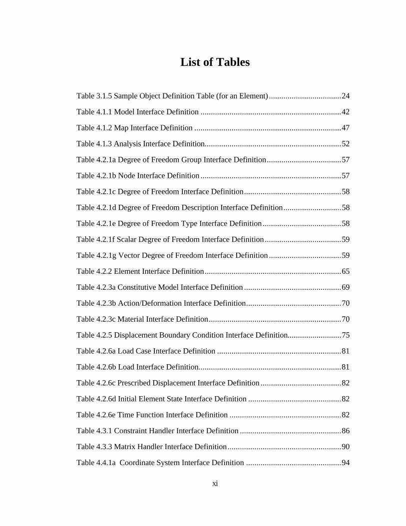
List of Tables..........................................................................................................xi
1. Introduction .......................................................................................................1
1.1 Problem.................................................................................................1
1.2 Objective..............................................................................................3
1.3 Object-Oriented Philosophy as a Solution..............................................4
1.4 Organization.........................................................................................5
2. Literature Review...............................................................................................7
2.1 G. R. Miller, et al...................................................................................10
2.2 T. Zimmermann, et al............................................................................11
2.3 Jun Lu, et al. ..........................................................................................12
2.4 J. W. Baugh, et al...................................................................................14
2.5 H. Adeli, et al.........................................................................................15
2.6 Discussion..............................................................................................16
3. Methodologies....................................................................................................19
3.1 Design Formalisms.................................................................................20
3.1.1 Design Intent...........................................................................20
3.1.2 Entity Relationship Diagrams...................................................20
3.1.3 Responsibility Description.......................................................21
3.1.4 Event Flow Diagram................................................................22
3.1.5 Interface Definition Table........................................................23
3.2 Implementation in C++..........................................................................24
3.2.1 Associations............................................................................25
iii

3.2.2 Inheritance...............................................................................26
3.2.3 Interfaces.................................................................................27
3.2.4 Libraries..................................................................................28
3.2.4.1 Container Classes......................................................29
3.2.4.2 Numerical Object Library..........................................30
3.3 Implementation Formalisms....................................................................30
3.3.1 C++ Interfaces.........................................................................31
3.3.2 Demonstration Code................................................................32
4. Object Model Design..........................................................................................35
4.1 Top Level Objects..................................................................................38
4.1.1 Model......................................................................................40
4.1.2 Map.........................................................................................42
4.1.3 Analysis...................................................................................48
4.2 Components of the Model......................................................................52
4.2.1 Degree of Freedom Group (Node)...........................................52
4.2.2 Element...................................................................................59
4.2.3 Material, Action/Deformation, and Constitutive Model............65
4.2.4 Constraint................................................................................70
4.2.5 Displacement Boundary Condition...........................................73
4.2.6 Load Case ...............................................................................75
4.3 Handlers................................................................................................82
4.3.1 Constraint Handler..................................................................83
4.3.2 Reorder Handler......................................................................86
4.3.3 Matrix Handler........................................................................89
4.4 Utility Objects........................................................................................91
4.4.1 Geometry................................................................................91
iv

4.4.2 Numerical Objects...................................................................95
4.4.3 Augmented Vector and Matrix Objects....................................98
5. Behavior of High Level Classes..........................................................................104
5.1 Element.................................................................................................106
5.1.1 Element Geometry...................................................................106
5.1.2 Communication of Element Properties.....................................107
5.1.3 Element State ..........................................................................109
5.1.4 Action/Deformation.................................................................110
5.1.5 Resisting Force........................................................................111
5.2 Constitutive Model................................................................................111
5.2.1 Material Data..........................................................................112
5.2.2 Action/Deformation.................................................................113
5.2.3 Constitutive Model State .........................................................115
5.3 Analysis.................................................................................................116
5.3.1 Analysis Constructors..............................................................117
5.3.2 Analysis State..........................................................................119
5.3.3 Assembly.................................................................................120
5.3.4 Treatment of Boundary Conditions..........................................121
5.4 Constraint Handler.................................................................................124
5.4.1 Transformation Theory............................................................124
5.4.2 Selection of Analysis Unknowns..............................................126
5.4.3 Data Types .............................................................................127
5.4.4 Implementation.......................................................................128
5.5 Map.......................................................................................................133
5.5.1 Example..................................................................................133
5.5.1.1 Transformation of a Stiffness Matrix.........................135
v

5.5.1.2 Processing of Responses..........................................138
5.5.2 Implementation.......................................................................139
6. Extensions and Examples.....................................................................................147
6.1 Examples of Analysis.............................................................................148
6.1.1 Linear Static Analysis..............................................................149
6.1.2 Nonlinear Static Event to Event Analysis.................................151
6.1.3 Nonlinear Static Analysis with Newton-Raphson Iteration.......155
6.1.4 Nonlinear Dynamic Analysis with Newton-Raphson
Iteration ...........................................................................................157
6.2 Substructuring ......................................................................................163
6.2.1 FeaSuperElement.....................................................................167
6.2.2 FeaSuperElementLoad.............................................................179
6.2.3 FeaSuperElementInitialState....................................................180
6.3 2D Beam Element With End Hinges......................................................181
6.3.1 Moment-Rotation Elastic-Perfectly Plastic Constitutive
Model ..............................................................................................182
6.3.2 2D Rectangular Coordinate System........................................191
6.3.3 2D Beam Element With End Hinges.......................................196
6.4 Building a Model...................................................................................215
6.5 Using the Finite Element Program..........................................................220
6.5.1 Linear Static Analysis..............................................................221
6.5.2 Nonlinear Static Analysis.........................................................222
6.5.3 Nonlinear Dynamic Analysis....................................................225
7. Conclusions and Future Work.............................................................................229
7.1 Conclusions...........................................................................................229
7.1.1 Architecture ............................................................................230
vi

7.1.2 Ease of Modification and Extendibility.....................................232
7.2 Future Work ..........................................................................................233
References...............................................................................................................236
Appendix: C++ Class Interfaces..............................................................................240
vii

List of Figures
Figure 3.1.2 Sample Entity Relationship Diagram....................................................21
Figure 3.1.4 Sample Event Flow Diagram (for a Node)............................................23
Figure 4.1 Overall Object Model..............................................................................38
Figure 4.1.1a Entity Relationship Diagram for the Model Object..............................40
Figure 4.1.1b Event Flow Diagram for the Model Object.........................................41
Figure 4.1.2a Entity Relationship Diagram for the Map Object.................................43
Figure 4.1.2b Event Flow Diagram for the Map Object............................................46
Figure 4.1.3 Event Flow Diagram for Analysis Class................................................51
Figure 4.2.1a Entity Relation Diagram for Degree of Freedom Group Objects.........54
Figure 4.2.1b Event Flow Diagram for the Degree of Freedom Group Object..........56
Figure 4.2.2a Entity Relationship Diagram for the Element Object...........................61
Figure 4.2.2b Event Flow Diagram for the Element Objects.....................................64
Figure 4.2.3a Entity Relationship Diagram for the Constitutive Model.....................67
Figure 4.2.3b Event Flow Diagram for the Constitutive Model Objects....................69
Figure 4.2.4a Entity Relationship Diagram for the Constraint Object........................71
Figure 4.2.4b Event Flow Diagram for the Constraint Object...................................72
Figure 4.2.5a Entity Relationship Diagram for the Displacement Boundary
Condition Object.....................................................................................................74
Figure 4.2.5b Event Flow Diagram for the Displacement Boundary Condition
Object.....................................................................................................................74
Figure 4.2.6a Entity Relationship Diagram for the Load Case Object.......................76
Figure 4.2.6b Event Flow Diagram for the Load Case Object...................................78
Figure 4.2.6c Event Flow Diagram for the Prescribed Displacement Object.............78
Figure 4.2.6d Event Flow Diagram for the Degree of Freedom Load Object............79
viii

Figure 4.2.6e Event Flow Diagram for the Element Load Object..............................79
Figure 4.2.6f Event Flow Diagram for the Initial Element State Object....................80
Figure 4.3.1a Entity Relationship Diagram for the Constraint Handler Object..........84
Figure 4.3.1b Event Flow Diagram for the Constraint Handler Object......................86
Figure 4.3.2a Entity Relationship Diagram for the Reorder Handler Object..............87
Figure 4.3.2b Event Flow Diagram for the Reorder Handler Object.........................88
Figure 4.3.3a Entity Relationship Diagram for the Matrix Handler Object................89
Figure 4.3.3b Event Flow Diagram for the Matrix Handler Object...........................90
Figure 4.4.1a Entity Relationship Diagram for the Geometry Objects.......................92
Figure 4.4.1b Event Flow Diagram for the Geometry Objects..................................93
Figure 4.4.2a Entity Relationship Diagram for the Numerical Objects......................96
Figure 4.4.3a Entity Relationship Diagram for the Augmented Vector and
Matrix Objects.........................................................................................................100
Figure 4.4.3b Event Flow Diagram for the Augmented Vector Object......................101
Figure 4.4.3c Event Flow Diagram for the Augmented Matrix Object......................101
Figure 5.5.1a Sample Problem.................................................................................134
Figure 5.5.1.1a Local Element Coordinate Systems and Transformation..................136
Figure 5.5.1.1b Nodal Coordinate Systems and Local-to-Nodal Transformation.....137
Figure 6.2a Entity Relationship Diagram for the Element Object..............................164
Figure 6.2b Internal and External Degrees of Freedom for a Submodel....................166
Figure 6.3.1b Elastic-Perfectly-Plastic Moment-Rotation Relationship.....................184
Figure 6.3.3a Entity Relationship Diagram for the 2D Beam Element with End
Hinges.....................................................................................................................196
Figure 6.3.3b Nodal Coordinate Systems................................................................198
Figure 6.3.3c External Element Coordinate Systems...............................................198
Figure 6.3.3d Internal Measures of Deformation.....................................................199
ix

Figure 6.3.3d Stiffness Transformation Matrix.........................................................205
Figure 6.4 Sample Model.........................................................................................216
Figure 6.5.1 Sample Problem: Holiday Inn, Van Nuys, Exterior Frame. Ref.
[23] .........................................................................................................................221
Figure 6.5.2a Top Floor Displacement.....................................................................224
Figure 6.5.2b Exterior Ground Floor Column End Moments....................................225
Figure 6.5.3a Sample Problem.................................................................................225
Figure 6.5.3b Top Floor Displacement.....................................................................227
Figure 6.5.3c Column Moments...............................................................................227
x
List of Tables
Table 3.1.5 Sample Object Definition Table (for an Element)...................................24
Table 4.1.1 Model Interface Definition....................................................................42
Table 4.1.2 Map Interface Definition.......................................................................47
Table 4.1.3 Analysis Interface Definition..................................................................52
Table 4.2.1a Degree of Freedom Group Interface Definition....................................57
Table 4.2.1b Node Interface Definition....................................................................57
Table 4.2.1c Degree of Freedom Interface Definition...............................................58
Table 4.2.1d Degree of Freedom Description Interface Definition............................58
Table 4.2.1e Degree of Freedom Type Interface Definition......................................58
Table 4.2.1f Scalar Degree of Freedom Interface Definition.....................................59
Table 4.2.1g Vector Degree of Freedom Interface Definition...................................59
Table 4.2.2 Element Interface Definition..................................................................65
Table 4.2.3a Constitutive Model Interface Definition...............................................69
Table 4.2.3b Action/Deformation Interface Definition..............................................70
Table 4.2.3c Material Interface Definition................................................................70
Table 4.2.5 Displacement Boundary Condition Interface Definition..........................75
Table 4.2.6a Load Case Interface Definition............................................................81
Table 4.2.6b Load Interface Definition.....................................................................81
Table 4.2.6c Prescribed Displacement Interface Definition.......................................82
Table 4.2.6d Initial Element State Interface Definition.............................................82
Table 4.2.6e Time Function Interface Definition......................................................82
Table 4.3.1 Constraint Handler Interface Definition.................................................86
Table 4.3.3 Matrix Handler Interface Definition.......................................................90
Table 4.4.1a Coordinate System Interface Definition..............................................94
xi

Table 4.4.1b Point Interface Definition...................................................................94
Table 4.4.1c Geometric Vector Interface Definition................................................94
Table 4.4.2a Vector Interface Definition..................................................................97
Table 4.4.2b Matrix Interface Definition..................................................................97
Table 4.4.3a Augmented Vector Interface Definition...............................................102
Table 4.4.3b Augmented Matrix Interface Definition...............................................102
Table 4.4.3c Transformation Interface Definition.....................................................103
Table 4.4.3d Transformation Description Interface Definition..................................103
Table 5.5.1a Mapping of Degrees of Freedom to Analysis Unknowns.....................135
Table 6.2a Element Interface Definition...................................................................165
Table 6.3.1a Constitutive Model Interface Definition...............................................183
Table 6.3.2a Coordinate System Interface Definition...............................................191
Table 6.3.3a Element Interface Definition................................................................197
xii

1. Introduction
Over the last 30 years, the finite element method has gained wide acceptance as a
general purpose tool for the modeling and simulation of physical systems. It has
become a crucial analytical technique in such diverse fields as structural mechanics,
fluid mechanics, electro-magnetics, and many others. As finite element techniques
evolve, the existing software systems must be modified. Therefore, finite element
analysis programs must be flexible.
1.1 Problem
Typical finite element programs consist of several hundred thousand lines of procedural
code, usually written in FORTRAN. The codes contain many complex data structures,
which are accessed throughout the program. This global decreases the flexibility of the
system. It is difficult to modify the existing codes and to extend the codes to adapt
1

them for new uses, models, and solution procedures. The inflexibility is demonstrated
in several ways: 1) a high degree of knowledge of the entire program is required to
work on even a minor portion of the code; 2) reuse of code is difficult; 3) a small
change in the data structures can ripple throughout the system; 4) the numerous
interdependencies between the components of the design are hidden and difficult to
establish; 5) the integrity of the data structures is not assured.
For the sake of efficiency, the various components of the program often directly access
the program's data structures. For example, elements, nodes, and constraints may need
to access the matrices and vectors involved in the analysis to obtain and transmit their
state information. This compounds the complexity of the components, by requiring
knowledge of the program's data structures. Modification or extension to a component
requires not only knowledge of the component at hand, but also a high degree of
knowledge of the entire program.
The components of the system become intimately tied to the program's data structures.
Access to the data structures occurs throughout the component, and easily becomes
inseparable from the component's function. Since the layout of the data structures is
unique to each program, the possibility of the reuse of the code in other systems is
greatly diminished. Also, code from other programs is difficult to adapt for use within
the system.
Since the data structures are globally accessible, a small change in the data structures
can have a ripple effect throughout the program. All portions of the code that access
the affected data structures must be updated. As a result, the layout of the data
2

structures tend to become fixed regardless of how appropriate they remain as the code
evolves.
The components of the system become dependent on each other via their common
access to the data structures. Little control can be placed on the access. As a result,
these interdependencies are numerous. More importantly, they are implicit. One
component can be completely unaware of another's reliance on the same data structure.
Thus, when modification or extension to a component occurs, it is difficult to assure
that all affected portions of the code are adjusted accordingly.
Access to the program's data structures is usually described by an interface. The
interface may merely consist of a document describing the layout of the data, or may
get as involved as a memory management tool that shields the data from the component
routines. In either case, it is up the each programmer to honor the interface. The best
laid plans are easily subverted for the sake of efficiency and ease of implementation.
1.2 Objective
Current finite element analysis software is inflexible and presents a barrier to practicing
engineers and researchers. Recoding these systems in a new language will not remove
this inflexibility. Instead, a redesign is needed. The objective of this dissertation is to
provide a new architecture for finite element analysis software which results in an
implementation that is manageable, extendible, and easily modified. The design will
provide the Civil Engineering profession with a flexible tool that can be adapted to
meet future requirements.
3

1.3 Object-Oriented Philosophy as a Solution
The application of object-oriented design has proven to be very beneficial to the
development of flexible programs. The basis of object-oriented design is abstraction.
The object-oriented philosophy abstracts out the essential immutable qualities of the
components of the finite element method. This abstraction forms a stable definition of
objects in which the relationships between the objects are explicitly defined. The
implicit reliance on another component's data does not occur. Thus, the design can be
extended with minimal effort.
The object-oriented paradigm provides four fundamental concepts [33, 9]; objects,
classes, inheritance, and polymorphism. Software is organized into objects that store
both its data and operators on the data. This permits developers to abstract out the
essential properties of an object; those that will be used by other objects. This
abstraction allows the details of the implementation of the object to be hidden, and thus
easily modified. Objects are instances described by a class definition. Classes are
related by inheritance. A subclass inherits behavior through the attributes and
operators of the superclass. Polymorphism allows the same operation to behave
differently in different classes and thus allows objects of one class to be used in place
of those of another related class.
The premise of this research is that the previously outlined problems with current finite
element programs can be eliminated by object-oriented design. The abstraction of the
data into objects limits the knowledge of the system required to work on the code to
4
only the object of interest and the services other objects provide to the object of
interest. Encapsulating the data and operations together isolates the classes and
promotes the reuse of code. Code reuse is further enhanced by placing attributes
common to several subclasses into the superclass, which is implemented once for all.
Changes to a class affect only the class in question. There is no ripple effect.
Interdependencies between the classes are explicitly laid out in the class interfaces. The
number of dependencies are minimized and easily determined. Object-oriented
languages enforce the encapsulation of the classes. The integrity of the data structures
is assured by the language.
1.4 Organization
The layout of this dissertation is described below.
Chapter 2: Literature Review - provides a survey of the current literature regarding
object-oriented finite element analysis design and programming.
Chapter 3: Methodologies - presents various methodologies that were used to
design, implement, and document the object-oriented finite element analysis
system.
Chapter 4: Object Model Design - provides a top-down, system level description of
the object model design. The primary focus of the chapter is the description of
abstractions for each class. The descriptions are given in terms of: the design
intent, which describes how the class fits into the system; an entity-relationship
5
diagram, which shows how the class is associated with other classes; a
responsibility description, which details the external and internal responsibilities
of the class; an event flow diagram, which outlines the flow of information for
the class; and the class interface definition table, which precisely defines the
methods the class provides to the system.
Chapter 5: Behavior of High Level Classes - describes the behavior of several
important high level objects in the system design. The chapter provides insight
into the implementation, without focusing on the details. The objects described
are the Element, the Constitutive Model, the Constraint Handler, the Map, and
the Analysis.
Chapter 6: Extensions and Examples - contains extensions to the basic finite
element analysis system described in the previous chapters, and examples that
demonstrate the use of the system. The extensions demonstrate that the design
is extendible. The examples include: a two-dimensional beam element with
hinges at the ends; a type of substructuring using the element interface; several
analysis types, including a nonlinear dynamic solution scheme using Newton-
Raphson iteration; and an example of the use of the program.
Chapter 7: Conclusions and Future Work - summarizes the research. Both the
significant findings and the direction of future research are discussed.
Appendix: C++ Class Interfaces - presents the public portions of the class interfaces
in the implementation.
6

2. Literature Review
The application of object-oriented design has only come to the structural engineering
community in the last several years. Several researchers began work in the late
eighties, leading to publication in the nineties. In 1990, Fenves [17] described the
advantages of object-oriented programming for the development of engineering
software. Namely, that its data abstraction technique leads to flexible, modular
programs with substantial code reuse.
One of the first detailed applications of the object-oriented paradigm to finite element
analysis was published in 1990 by Forde, et al. [19]. The authors abstracted out the
essential components of the finite element method (elements, nodes, materials,
boundary conditions, and loads) into a class structure used by most subsequent authors.
Also presented was a hierarchy of numerical objects to aid in the analysis. Other
authors [18, 24, 29, 30] increased the general awareness of the advantages of object-
oriented finite element analysis over traditional FORTRAN based approaches.
7

Some researchers have concentrated on the development of numerical objects. Scholz
[34] gives many detailed programming examples for full vector and matrix classes.
Zeglinski, et al. [40] provide a more complete linear algebra library including full,
sparse, banded, and triangular matrix types. Also included is a good description of the
semantics of operators in C++. Lu, et al. [22] present a C++ numerical class library
with additional matrix types such as a profile matrix. They report efficiency
comparable to a C implementation. Lu, et al. weakly argue against using the standard
FORTRAN library LAPACK [2] by noting that "[LAPACK does] not embody the
principles of encapsulation and data abstraction". Dongarra, et al. [13] present an
object-oriented (C++) version of LAPACK named LAPACK++. It includes full,
symmetric, and banded matrix types, and, according to the authors, the library can be
extended to include other types. They report speed and efficiency competitive with
native FORTRAN codes.
Rihaczek, et al. [31] present a short paper showing some abstractions for a heat
transfer type problem. An interesting component of their design is the Assemblage
class which coordinates the interaction between the model and the analysis. It contains
the topological buildup, the constraints, and the loads. Chudoba, et al. [8] present a
similar type of Connector class, to exchange data between elements and the analysis.
The concept of an object responsible for the mapping between the model and the
analysis is echoed by Lu, et al. [22, 7, 35].
One of the most complete treatments of material class, the modeling of the constitutive
relationships, is presented by Zahlten, et al. [39, 20]. A particular material object is an
assemblage of a yield surface object, a hardening rule object, a flow rule object, and an
8

algorithm to solve the initial value problem. The material object itself tracks the state
of strain and directs the calculation of stress.
The focus of this dissertation is the development of a complete finite element system
architecture. The remainder of this chapter presents five such systems that exist in the
literature. Each architecture is evaluated with respect to the following significant
criteria:
• Nodes: The information stored at the nodes and the manner in which the
degrees of freedom are represented.
• Elements: Communication of element properties and use of constitutive
models.
• Constitutive Models: Integration with the element class.
• Constraints: Representation and handling of single and multi-point
constraints.
• Geometry: Support for multiple coordinate systems, and representation of
tensors.
• Transformations: The handling of data transformation from one basis to
another.
• Mapping from the Model to the Analysis: The handling of the mapping
between the model degrees of freedom and the final equations of equilibrium.
• Analysis: The types of analyses that are presented.
• Numerical objects: The set of classes provided for vector and matrix algebra.
9

2.1 G. R. Miller, et al.
G. R. Miller, et al. [26, 27, 28] present an object-oriented software architecture for use
in nonlinear dynamic finite element analyses. The system is based on a coordinate-free
geometry, which includes points, vectors, and tensors in three dimensions. No mention
is made of supporting numerical work. No specific solution schemes are given, but the
intention of the work is to allow for iterative element-by-element solution methods.
Transformations are handled by the coordinate-free geometry. Since all element and
nodal properties are formulated without reference to a specific coordinate system, the
elements and nodes do not participate in the transformation process. Elements report
their properties in terms of geometric vectors and tensors. No information is given as
to how these are transformed into numeric vectors and matrices for solution. Since the
work is intended for an element-by-element solution algorithm, no mapping between
the model and analysis equations of equilibrium is provided. As a result of the
coordinate free geometry, an element can be used in 1, 2, or 3D problems, regardless of
its internal representation.
The material objects provide the constitutive relationships to the elements. The
relationship can be nonlinear and path dependent. The material is responsible for
maintaining its own state. Stress and strain are reported as tensors.
The nodes are positioned in space using the geometric points. Nodes hold collections
of scalar and vector degrees of freedom. The information stored at the degrees of
freedom varies according to the solution scheme. Each scheme requires a different
subclass of degree of freedom. Loads are applied to the nodes, and can vary with time.
10

Constraints also apply directly to the nodes by "absorbing force components from
constrained directions" [28]. No details of the constraint handling procedure are given.
2.2 T. Zimmermann, et al.
T. Zimmermann, et al. [14, 15, 25, 2] have developed a software architecture for linear
dynamic finite element analysis, with extensions to account for material nonlinearity.
The nonlinear extension required the redefinition of some of the original classes. The
system is similar to traditional finite element analysis programs in that all data stored is
in terms of global degrees of freedom, and the properties of a structure as a whole are
assembled into a system of linear equations. Transformations are performed implicitly
by the object that creates the information. No geometric classes are defined to aid in
element geometry and vector based data manipulation. A basic numerical library is
provided which contains full, banded, and skyline matrices and full vectors.
The system of linear equations is contained within a subclass of the LinearSystem class.
The subclassing is based on the storage scheme used for the system stiffness and mass
matrices. The LinearSystem objects are responsible for equation numbering, some
assembly tasks, and the production of the response quantities. With the exception of
the simple displacement boundary conditions, there is a one-to-one mapping between
degrees of freedom and equations of equilibrium.
Elements produce stiffness and mass matrices and equivalent load vectors in terms of
the global coordinates at the nodes. Elements do not provide a damping matrix. All
nodes have the same set of coordinates defining the direction of the degrees of
11

freedom. The elements are responsible for the assembly of their properties into the
global property objects with the help of the LinearSystem object. The elements define
and manage their own constitutive models. A material class is provided to handle
material properties such as Young's Modulus and mass density.
The nodes store their physical location, in terms of global coordinates, a list of degrees
of freedom, applied loads, and the location of the degrees of freedom in the global set
of equations of equilibrium. The degrees of freedom can retrieve their response values
(displacements, velocities, and accelerations) from the global response vectors. The
nodes also keep track of their displacement boundary conditions. No multi-point
constraints are provided. The equation numbers associated with the degrees of
freedom are obtained by the node from the LinearSystem object.
The extensions to the system to accommodate material nonlinearity required the
redefinition of some classes and the addition of others. Most significantly, was that of
a Domain class, which steps the LinearSystem objects through a Newton-Raphson
iteration scheme to convergence. Other objects, such as the GaussPoint, Material, and
Element class, were redefined to permit nonlinear behavior.
2.3 Jun Lu, et al.
Jun Lu, et al. [22, 7, 35] present an excellent architecture for a small, flexible, "fly-
weight" finite element analysis program. The heart of the system is an Assembler
object, which performs the transformation of element properties between the element
coordinates and the structural degrees of freedom. The Assembler object also assigns
12

equation of equilibrium numbers to the structural degrees of freedom and builds the
structural property matrices. Few details are given.
A large numerical library was developed by the authors. It includes banded, triangular,
sparse, symmetric, and profile matrices.
Although no set of geometric support objects are given, reference to coordinate
systems and tensors indicate that at least a rudimentary system is implicit in the design.
The elements provide their local coordinate systems, and the nodes provide the
structural coordinate systems, to the Assembler.
Elements can provide their stiffness, mass, and damping matrices. No facilities for state
update or resisting force calculations are provided. Element forces are communicated
to the Assembler as equivalent nodal loads to be included in the right hand side of the
equation of equilibrium. A material class is available to provide the elements with a
basic stress-strain law. The element is responsible for using this to derive the
appropriate constitutive equations, such as moment-curvature, as needed. Nonlinear
material objects are permitted, but no details are given.
The nodes contain their position in space, and a collection of degree of freedom
objects. The degrees of freedom consists of a vector in a coordinate system. The
direction of the vector indicates the direction of the degree of freedom (for example,
three degrees of freedom are required for 3D translation). The associated equation
number, assigned by the Assembler, is stored in the degree of freedom. Only single
point constraints are permitted. The constraint information is contained in the degree
of freedom.
13

No solution schemes are provided, but an EquationSolver class is given. Its subtype
seems to be determined by the storage type chosen for the structural property matrices.
The communication between the EquationSolver and the Assembler, which appears to
be highly dependent upon the matrix type chosen, is not described.
2.4 J. W. Baugh, et al.
J. W. Baugh, et al. [3, 4] present an architecture for a linear static finite element
analysis program. The bases of the system is the coordinate system objects which
permit the elements and nodes to describe themselves in terms of Cartesian, Cylindrical,
and Spherical systems. The coordinate systems are related to a global coordinate
system by a 3x3 rotation matrix (direction cosines). These rotation matrices are used
to perform the transformations of load vectors and stiffness matrices from one
coordinate system to another.
Each node stores its position in its own coordinate system. The same coordinate
system is used to describe the orientation of the degrees of freedom at the node. Both
rotations and translations use this same system. The displacements calculated by the
analysis are stored at the nodes. The degrees of freedom maintain their boundary
condition and loading value. Only single point constraints are permitted. The nodes
also store the topology of the model, that is the connectivity caused by the elements.
The elements are responsible for obtaining the coordinate systems at the nodes, and
transforming their stiffness and load values into these nodal coordinates using the
14

rotation matrices provided by the coordinate systems. The elements are required to
assemble themselves into the global stiffness matrix and load vector. No details for this
process are provided. A material class is given to provide the constitutive model for
the element. The material objects are subclassed according to the measures of stress
and strain used in the material interface.
2.5 H. Adeli, et al.
H. Adeli, et al. [1, 38] present a simple linear elastic static finite element system that is
closely related to traditional finite element programs. All nodes have three
displacement degrees of freedom. The orientation of these degrees of freedom
coincides with the assumed global coordinate system. No information is provided as to
how the equations of equilibrium are formed, or their relation to the degrees of
freedom. No facilities for geometric support or transformations are provided. A small
numeric library is developed which includes full vector and full matrix classes.
A separate class, named GlobalData, is created to make some model parameters, such
as the number of degrees of freedom, available to all objects in the system. Some
classes use the GlobalData class as a superclass "to provide better service".
The nodes store their position in the global coordinate system. They also store the
value of the displacements of their three degrees of freedom. Nodes can be subclassed
based on geometry to aid in the generation of the nodes. A DNode class is a subclass
of the Node class, and is used to represent an increment in the coordinates from one
node to another.
15

Only linear elastic elements are permitted. The classes Shape, Gauss, and Jacob are
provided to aid in the element formulation. An Element_seq class is also given to
provide information to the element regarding the sequence of nodes to which the
element attaches. A material class is also provided, but no details are given.
2.6 Discussion
The five system architectures reviewed demonstrate the wide range of views on object-
oriented finite element program design. A recurring theme is the desire to isolate the
various components of the system from one another. The most successful at this is Lu,
et al., with their creation of the Assembler class, which attempts to isolate the model
from the analysis. Significant drawbacks to their approach are the assumption of the
one-to-one correspondence between model degrees of freedom and equations of
equilibrium, and the fact that the equation number is stored at the node. Multi-point
constraints would be extremely difficult to add to the system, and the presence of the
analysis equation numbers within the model may lead to implicit reliance on analysis
data with model components.
Both Miller, et al. and Baugh, et al. provide geometric objects in support of the
system. This approach not only frees programmers from the transformation task, but
this centralized approach encourages efficient implementation of these basic objects.
One drawback to Miller's insistence on the use of tensors is that it tends to dissuade
future development of the system by researchers more comfortable with traditional
matrix structural analysis. Perhaps a better approach is to include both tensor and
16

matrix representation. Baugh's approach of relying on the coordinate system objects to
provide the transformation matrices seems appropriate.
Since most additions to existing finite element codes involve new elements, it is
desirable to reduce the work of the element authors as much as possible. Most systems
demand that the element provide its properties in terms of the nodal coordinate
systems. This creates additional work for each element writer. With Miller's
coordinate free geometry, this is eliminated, but at the expense of a tensor formulation.
It is preferable to allow the element to provide its properties in any form, but then insist
that the element provide a transformation into a convenient set of local coordinate
systems recognizable to the rest of the system.
The treatment of constraints in the five systems, for the most part, appears to be an
after-thought. Only single point constraints are permitted. These are generally stored
as an attribute of the degree of freedom. This eliminates the seamless inclusion of the
multi-point constraints types used in most existing finite element programs.
Upon discovery of object-oriented programming languages, one of the engineer's first
thoughts is the application of inheritance to matrices. The ability to seamlessly switch
the basic matrix storage scheme and solver in a finite element system is very attractive.
As a result, most of the systems have developed their own numerical libraries. This
repetition of work is inefficient. The use of a universally available, efficienct, numerical
library is preferable. The design of the library is best left to specialists in numerical
analysis [2, 13]. This frees engineers to concentrate on the structural aspects of the
design.
17

Some items that are typically included in existing finite element programs are missing
from the above systems. This is probably due to the lack of space available in a
publication, but they do deserve note. Loads should be grouped into load cases, and
the load cases grouped into load combinations. Prescribed displacements should be
included in the load cases. Renumbering of the equations of equilibrium to reduce the
solution cost should be provided. Provision for substructuring is also very useful.
18

3. Methodologies
This chapter presents the methodologies that were used to design, implement, and
document the object-oriented finite element analysis system. It is divided into three
sections: Design Formalisms; Implementation in C++; and Implementation
Formalisms. The design formalisms are the means by which the object design was
created, and also the methods used to document the design. The design was
implemented in the C++ programming language. The implementation in the C++
section describes the general manner in which the implementation was developed in
C++. The final section describes the C++ interfaces for the implemented classes
contained in the Appendix, and the demonstration code that appears throughout the
dissertation.
19

3.1 Design Formalisms
Object modeling is iterative by nature, as is any design activity. The principal tool used
throughout the design process is the Entity Relationship Diagram, which shows the
relationships between the classes. While this tool is useful in the design process, it does
not provide complete information for the description of the final design. In this section,
the description of the object model design includes the Design Intent, an Entity-
Relationship Diagram, a Responsibility Description, an Event Flow Diagram, and the
Interface Definition Table.
3.1.1 Design Intent
The Design Intent of a class is a top-level description of what place the class occupies
in the overall object design. It describes the purpose of the abstraction and the inherent
qualities of the class. The description is not in reference to any programming concept,
but to the actual purpose the class fulfills in the finite element method. For example,
the design intent of an element is to represent the physical properties of the piece of the
model it describes, and maintain the state of those properties.
3.1.2 Entity Relationship Diagrams
Entity Relationship diagrams are commonly used (Rumbaugh [33]) to show the
relationships among classes in the design. A sample Entity Relationship Diagram is
shown in Figure 3.1.2. Classes are shown as boxes around the class name. The links
between the boxes establish the relationship between the classes. Links are labeled
20

with the type of association that exists between the classes. In the example, an Element
connects to a Node. Thus, the classes Element and Node are linked together with the
connects to association. In fact, many Elements may connect to many Nodes. This
multiplicity, of zero or more, is represented by a darkened circle at the end of the link.
Links with no special ending represent a multiplicity of exactly one. Links that end in a
diamond shape represent aggregation. Aggregation describes a relationship in which
one object is part of another in an assembly. For instance, many Nodes and many
Elements are part of a Model. Generalization is represented by a triangle within a link
pointing towards the more general class. For example, the Element class is a
generalization of a Truss Bar, a 27-Node Brick, and other classes represented by the
dots.
connects toElement
...Truss Bar 27-Node Brick
Model
Node
Figure 3.1.2 Sample Entity Relationship Diagram
3.1.3 Responsibility Description
The Responsibility Description is used to show the features the class is responsible for
providing to other objects, and also what actions the class performs internally to meet
21

these responsibilities. The responsibilities are the embodiment of the design intent.
They show how the object will satisfy the design intent to the rest of the system. The
design intent for an Element may state that the Element provides its stiffness to the
Analysis. The responsibility description, on the other hand, describes how the Element
queries its Constitutive Models to determine the current stiffness and passes this on as a
matrix augmented with transformations.
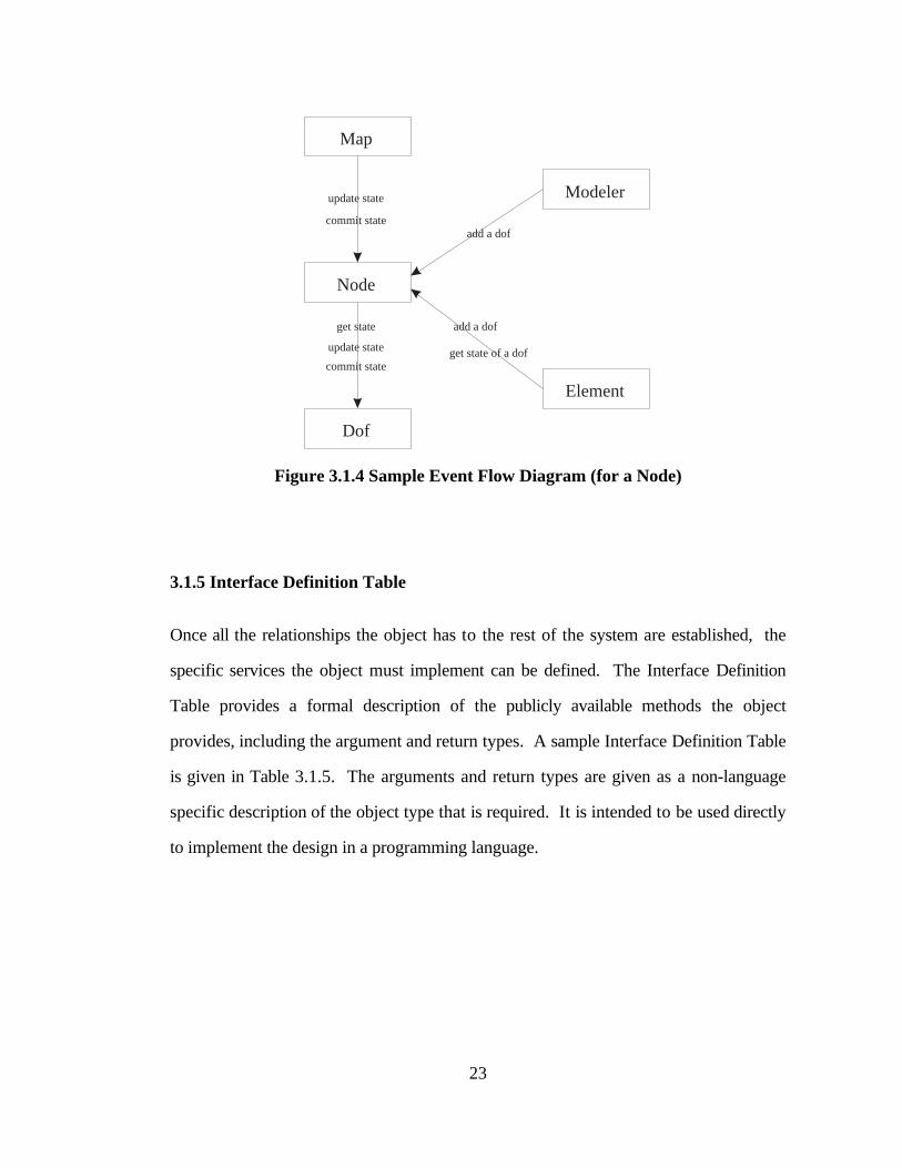
3.1.4 Event Flow Diagram
An Event Flow Diagram shows the methods provided to the clients of the class, and
which features of other classes are used to perform these functions. A sample Event
Flow Diagram for a Node is given in Figure 3.1.4. For clarity, not all events are
shown. The diagram shows the events that may occur between the classes. Events are
the flow of information between objects. Events that flow toward the class in question
represent services the class must provide. Events that flow away represent services of
other classes that are required. Classes are represented by boxes containing the class
name. The links between the boxes represent events. The arrow on the link points
away from the object that initiates the event. For example, a degree of freedom (Dof)
can be added to a Node by the Modeler or an Element. A Map can update and commit
the state of the Node. The Node in turn updates and commits the state of its degrees
of freedom. An Element can request the state of a particular degree of freedom from
the Node. The Node gets the state from the degree of freedom in question.
22
commit state
add a dof
Element
update state
commit state
Node
Modeler
Dof
Map
add a dof
get state of a dofupdate state
get state
Figure 3.1.4 Sample Event Flow Diagram (for a Node)
3.1.5 Interface Definition Table
Once all the relationships the object has to the rest of the system are established, the
specific services the object must implement can be defined. The Interface Definition
Table provides a formal description of the publicly available methods the object
provides, including the argument and return types. A sample Interface Definition Table
is given in Table 3.1.5. The arguments and return types are given as a non-language
specific description of the object type that is required. It is intended to be used directly
to implement the design in a programming language.
23

Method Arguments Return PurposeConstruction Unique to each element, but
includes instances of
Constitutive Models
Creates an instance of a
specific type of Element
getStiff Stiffness matrix augmented
with transformation into
known Coord Sys
Provides the current linearized
stiffness
getDamp Damping matrix augmented
with transformation into
known Coord Sys
Provides the current Damping
matrix
getMass Mass matrix augmented with
transformation into known
Coord Sys
Provides the current Mass
matrix
getResistingForce Load vector augmented with
Coord Sys
Provides the current resisting
force, including the initial state
and element loads
updateState Causes the Element to update
its state from the Nodes
getEventFactor Event Factor Returns the current event
factor
initialize Unique to each type of
Element
Announces the presence of an
Initial Element State
commitState Commits the current state of
the Element
getConnectingDof list of dof Returns a list of dof to which
the element attaches
Table 3.1.5 Sample Object Definition Table (for an Element)
3.2 Implementation in C++
Once the object design is complete, the next task is implementation in a computer
language. The natural choice for an object-oriented design is an object-oriented
programming language. There are many object-oriented languages available, and each
has its own set of features and quirks. C++ [16, 37] was chosen. The implementation
specifications are given, in the form of the C++ public interfaces for the classes, in the
Appendix.
24
C++ is the most widely used object-oriented programming language for a wide range of
applications. Specifically, in the object-oriented finite element literature reviewed in the
previous chapter, virtually all authors based their work on C++. Such a large base of
users has led to many high quality compilers, container class libraries, and numerical
object libraries. For the most part, C++ is compatible with the C programming
language. Thus, old C code and even older C programmers can be incorporated with
minimal effort. When designed properly, C++ code is as fast and memory efficient as C
code.
The objects described, using the design formalisms from the previous section, lend
themselves to direct implementation as classes in C++. The Design Intent and
Responsibility Description define the abstraction the class encompasses. The Entity
Relationship Diagram and Event Flow Diagrams give the inheritance relationship and
other dependencies the class has with other classes. The Interface Definition Table
defines the methods the class must provide. What remains at the discretion of the
implementation are the specific C++ data types used as the arguments and return values
of the methods, and the data types used for the class's instance variables.
3.2.1 Associations
Associations between classes can be implemented as pointers, friends, and distinct
association objects. A pointer references another object as an instance variable in the
class. Access to the public methods of the referenced object is available. This is
appropriate for a one-to-one association; the pointer may reside in either class. For a
one-to-many association, a list of pointers may be employed at the end with a
25

multiplicity of one. For more complex associations, such as many-to-many
associations, where access from each side of the association is required, a distinct
association object may be used. This type of association, typically used in database
applications, did not come up in the research. All associations are implemented as
pointers.
3.2.2 Inheritance
The implementation of the inheritance relationships in the object design is fairly
straightforward in C++. A subclass inherits from one or more superclasses. The
decision as to which features of the superclass the subclass may inherit, are decided in
the implementation of the superclass. In C++, this is declared by the use of private,
public, protected, and virtual members. The private members of the superclass are
hidden from the subclass. Only the public and protected members are available to the
subclass. Declaring a member private preserves encapsulation, but limits the usefulness
of future subclasses. Methods that are declared virtual in the superclass may be
replaced in the subclass. For example, a print method for a superclass can be replaced
by a print method in the subclass. Declaring a method to be virtual in a class enhances
the flexibility of future subclasses.
An abstract class is one in which an instance of the class cannot exist. Its purpose is to
serve as a superclass to a number of subclasses. For example, the class Element is
abstract and serves as the superclass for all element types such as Truss Bar. An
abstract class is indicated by the presence of a method that is declared pure virtual. A
26

pure virtual method has no implementation. The method must be implemented in the
subclass.
3.2.3 Interfaces
In C++, the instance variables and method prototypes of a class are typically declared
together as the interface for the class. C++ is a statically typed language, so the type of
all variables must be declared in the interfaces. The interface for the class provides an
excellent means to describe the implementation. The available methods in the actual
interface for a class may differ slightly from the Object Definition Table given in the
design. Additional methods may be provided for implementation specific tasks, such as
providing a hash function for the object. A typical interface is:
class FeaNode : public FeaDofGroup {private:
FeaGeoPoint* location; // location of the nodepublic:
// constructorFeaNode(char* name, FeaGeoPoint& point);
// copy constructorFeaNode(FeaNode& other);
// destructor~FeaNode();
// assignment operatorvoid operator=(FeaNode& other);
// get position of the nodeFeaGeoPoint& getPosition();
// print out the nodevoid print();
};
27

This is the interface for the class FeaNode. The first line declares that FeaNode inherits
from the class FeaDofGroup, and the public interface of FeaDofGroup is included in the
interface for FeaNode. The instance variable location , is pointer a object of type
FeaGeoPoint. This instance variable is private.
In this example, there are six publicly available methods. The first two methods are
constructors, as they have the same name as the class. Constructors are used to
construct an instance of the class FeaNode. The first method has two arguments, a
pointer to a character, and a reference to an object of type FeaGeoPoint. The second
method is a copy constructor. It creates an instance of type FeaNode that is an exact
copy of the referenced object. The third method is the destructor for the class. It can
be called explicitly to remove an instance of the class, or implicitly by the compiler
when an instance of FeaNode falls out of scope. The fourth method defines the
assignment operator for the class. These four types of methods will appear in all class
interfaces. The last two methods complete the interface for the FeaNode class. The
position of the node is returned by reference, and an instance of FeaNode can be
instructed to print itself.
3.2.4 Libraries
The implementation of the object design requires the use of specific C++ classes to
serve as the arguments and return values of the methods. Most classes will be defined
in the object design or taken from a library of numerical objects; others are taken from
the intrinsic C++ types, such as ints and doubles . Often a class will make use of
complex data structures typically referred to as container classes.
28

3.2.4.1 Container Classes
The container classes used in the implementation are: vectors, lists, dictionaries, tables,
and combinations of the four. An array is a fixed-length collection of objects of the
same type. Value access is through an integer index. Individual members of the
collection are accessed directly. Access is rapid, but the number of members in the
collection must be known ahead of time. The list data structure is a singly linked list of
a specific class of objects capable of adding new objects to the front or back of the list,
and providing an iterator for sequential access to the elements of the list. To access a
specific element on the list, the list must be traversed until the element is found. Access
is slow, but the size is not fixed. A dictionary is a list of pairs of keys and values.
Access to a value is obtained using the key as an index. The internal representation for
this implementation is a list, so the search for a specific key is slow. A table
implements the collection of pairs of keys and values as a hash table. Access to a
specific key is faster then for a dictionary, but a hash function must be provided for the
key object.
The data structure library detailed by T. Budd [6] was selected for use in the program.
The code is well documented. As a result, it is easy to use and understand. Near the
end of the programming portion of the research, the ANSI/ISO C++ Standard
Committee voted to make the Standard Template Library (STL) [36] part of the
standard C++ library. The committee's work is not final, and the STL does not work
all compilers due to its heavy use of templates. The STL contains the necessary data
structures, and will be included in the next revision to the finite element program.
29

3.2.4.2 Numerical Object Library
The purpose of the numerical object library is to provide a useful set of general and
specialized vectors and matrices in support of the finite element program. The
literature contains many examples of libraries of matrices, some by authors of finite
element programs [22, 40, 34], others by numerical analysts [13, 2]. The selection of a
numerical object library is not to be taken lightly, as it affects many aspects of the
system. To begin the selection, one needs to define what is required from the library.
In this work, a minimal numerical object library is used. Typical vector operations such
as transposition and multiplication, and matrix operations, such as eigen-analysis, are
not implemented. The numerical objects could be subclassed based on sparsity. For
the arrays, only the full array has been implemented. For the matrices, the
implementations for the full and block matrices are given.
3.3 Implementation Formalisms
The complete C++ code for the implemented object design consists of over 10,000
lines. Obviously it is far too bulky to be presented in this document. Some code is
presented to help understand, use, and extend the program. Chapter 5 gives a detailed
explanation of some of the top level objects in the program, and Chapter 6 presents
some objects that were added to the design. The C++ interfaces for the classes are
given in the Appendix. This section describes the formalisms used in the Appendix and
Chapters 5 and 6. Namely, an explanation of the public interfaces for the classes, and a
description of the code used to demonstrate the implementation.
30
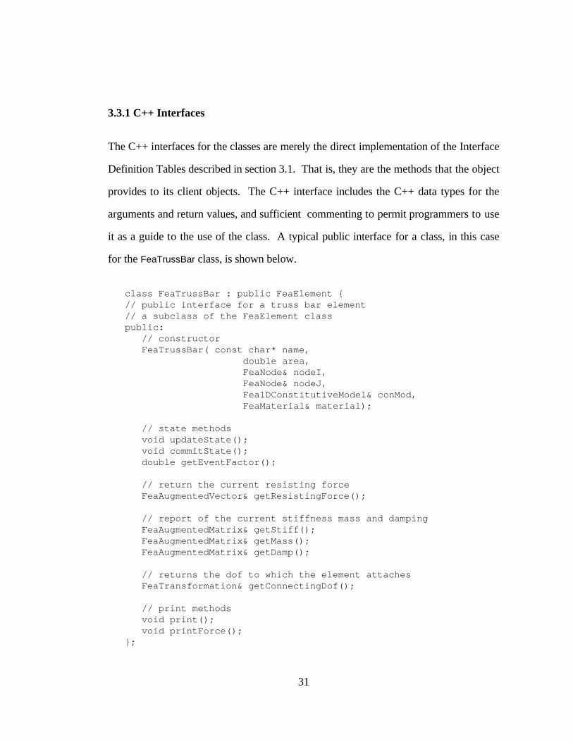
3.3.1 C++ Interfaces
The C++ interfaces for the classes are merely the direct implementation of the Interface
Definition Tables described in section 3.1. That is, they are the methods that the object
provides to its client objects. The C++ interface includes the C++ data types for the
arguments and return values, and sufficient commenting to permit programmers to use
it as a guide to the use of the class. A typical public interface for a class, in this case
for the FeaTrussBar class, is shown below.
class FeaTrussBar : public FeaElement {// public interface for a truss bar element// a subclass of the FeaElement classpublic:
// constructorFeaTrussBar( const char* name,
double area,FeaNode& nodeI,FeaNode& nodeJ,Fea1DConstitutiveModel& conMod,FeaMaterial& material);
// state methodsvoid updateState();void commitState();double getEventFactor();
// return the current resisting forceFeaAugmentedVector& getResistingForce();
// report of the current stiffness mass and dampingFeaAugmentedMatrix& getStiff();FeaAugmentedMatrix& getMass();FeaAugmentedMatrix& getDamp();
// returns the dof to which the element attachesFeaTransformation& getConnectingDof();
// print methodsvoid print();void printForce();
};
31

A comparison of this C++ interface with the Interface Definition Table, shown
previously as Table 3.1, shows the direct relationship between the class as designed and
as implemented. The first line of the public interface names the class as FeaTrussBar,
which is a subclass of FeaElement. Following this declaration, are the public methods
of the class. The names of the methods are preceded by the type of the return value.
The arguments for the methods are contained with brackets and include the argument
type and a name with indicates the meaning of the argument. Two print methods are
included to output the state of the element.
3.3.2 Demonstration Code
Code fragments are used throughout Chapters 5 and 6 to demonstrate the
implementation. The reason for the demonstration code is that actual C++ code
involves somewhat complicated syntax to declare data types and memory management.
The principal differences with C++ are: data types are not declared when they can be
inferred from the context of the use; use of pointers or references are implicit;
memory management is not included; iteration through data structures is simplified;
and method calls are not chained together for clarity. For a description of the C++
language, the reader is directed to the literature [16, 37, 9].
Where the type of a variable is clear from the context of the statement, the type
declaration is not included in the demonstration code. For example, in the C++
statement:
FeaFullMatrix* el = new FeaFullMatrix(3,3);
32

creates a 3 by 3 matrix (FeaFullMatrix) and a pointer to it named el . The
demonstration code for this is:
el = new FeaFullMatrix(3,3);
The type for el can is implied from the statement without the explicit declaration. All
variables are treated as values. This clarifies the syntax a little by avoiding the
referencing, de-referencing, and deletion of variables. In C++, the component of el on
the second row and third column is referred to as (*el)(1,2) , whereas in the
demonstration code, the fact that el is a pointer is not shown, therefore the element is
accessed as el(1,2) .
A common operation in the program is to iterate through a collection of objects. The
collection may be a list, vector, dictionary, or table. The syntax for this can be quite
cumbersome. The type of the iterator must first be declared, the iterator is then
obtained from the collection, and a for loop is set up to iterate through the collection.
For example, the C++ code to iterate through the components of a hash table named
map is:
// declaration for maptable< FeaDofCompDesc&, dictionary<int, double> > map;
// declare iterator using map in the constructortableIterator< FeaDofCompDesc&, dictionary<int, double> >itr(map);
// initialize and loop through itrfor ( itr.init(); ! itr; ++itr ){}
The demonstration code for the creation of the iterator is shown as a call on the map's
getItr method. The loop is shown as iterateThrough demonstration code
statement acting on itr .
33

// declare iterator using map in the constructoritr = map.getItr();
// initialize and loop through itriterateThrough( itr ){}
The important features of the code have been captured; that is, the source of the
iterator and the presence of the loop. In both C++ and demonstration code, the ()
operator yields the current item in the collection.
34

4. Object Model Design
This chapter presents a top-down, system level description of the object model design
for the Object-Oriented Finite Element Analysis Program. The essence of this design is
abstraction. That is, the identification of the essential properties of the classes of
objects, and thus the division of responsibilities between the classes. Therefore, the
primary focus of the chapter is the description of abstractions for each class. The
description does not deal with the implementation of the classes. The details of how
the responsibilities will be met are described in subsequent chapters.
The intent of the object design is to form a set of abstractions for the Finite Element
Method that are flexible enough to permit the addition of yet unenvisioned concepts.
Only the inherent qualities of the objects must be defined in the abstractions. Since
these qualities will not change, additional features can be incorporated into the system
without requiring change to the existing object design, only additions.
The names of the objects in the design are based on the function they fulfill in the finite
element method. A Model object represents the finite element model, an Analysis
35

object represents the numerical description of the analysis, and the Map object provides
the mapping between the model and the analysis. A model is composed of elements,
nodes, constraints, and loads. Elements form the foundation of the finite element
method. An Element object provides the properties of the portion of the model it
physically represents. Elements attach to Nodes. Node objects represent a point in
space and contain Degrees of Freedom objects, which represent the unknowns of the
problem. A Constraint object is a time invariant homogeneous multi-point constraint in
the model (such as rigid body constraints). A Displacement Boundary Condition object
represents a single-point constraint that can vary in time. A Load Case object consists
of possibly many Load objects, Prescribed Displacement Value objects, and Initial
Element State objects, that together form a set of loads on the model. The Load
objects may apply to nodes or elements.
The basic features of the design are as follows: The state of the model to be analyzed
is represented in the Model, in terms of degrees of freedom and elements. The Analysis
deals mostly with numerical objects (Vectors and Matrices) in terms of analysis
unknowns. The Map provides the link between degrees of freedom in the Model, and
unknowns in the Analysis. All objects passing between the Analysis and the Model,
and vice versa, must go through the Map for transformation. Provision is made for
analysis unknown reordering. Homogeneous multi-point constraints are contained in
Constraint objects, and are processed by a Constraint Handler. Single-point constraints
can be non-homogeneous and time dependent, and are processed directly by the
Analysis. Coordinate System, Vector, and Point objects are provided. All Coordinate
System objects can produce transformations to all other Coordinate Systems, including
those with a different number of dimensions. Vectors and Points contain their own
internal Coordinate System. Nodes store response data at the degrees of freedom as
36

Scalars or Vectors. Elements retrieve information from the Nodes as Scalars and
Vectors and may interpret them in any convenient Coordinate System. Elements of a
certain dimension (such as a one-dimensional truss bar) may be placed in a problem of a
different dimension (such as a three-dimensional system). Transformation of vectors
and matrices from element to local to nodal to analysis unknowns and vice versa are
handled using augmented vectors and matrices that take advantage of the block
structure of the transformations, and apply all the pending transformations efficiently
only when the final value is needed.
Elements and Loads may express their properties in any convenient Coordinate System.
Transformation to nodal degrees of freedom and further into analysis unknowns is
handled by the Map. Both Nodal and Element Loads are provided, and are separated
into Load Cases.
The chapter is divided up into several subsections. Each subsection deals with one or
more closely related classes that together form a module for a specific purpose. As
described in the previous chapter, the descriptions of the Object Model Design are
given in terms of: the Design Intent, which describes how the class fits into the Finite
Element Method; an Entity-Relationship Diagram, which shows how the class is
associated with other classes; a Responsibility Description, which details the external
and internal responsibilities of the class; an Event Flow Diagram, which outlines the
flow of information for the class, and the Interface Definition Table, which precisely
defines the public methods of the class.
37

4.1 Top Level Objects
To provide a general overview of how the components of the object design fit together,
Figure 4.1 gives the basic layout of the object model. Class names are shown within
boxes, and the associations between the classes are drawn as lines connecting the
boxes. The notation is similar to an Entity Relationship Diagram described by
Rumbaugh et al [33], but only a few of the principal classes and associations are
shown. At this high level, the system design consists of a Model, an Analysis, a Map,
and two Handlers.
has a
has a
initializes
queries
reorders
has a
queries
Map Reorder Handler
represents
Constraint Handler
Model
Analysis
Figure 4.1 Overall Object Model
An Analysis object performs an analysis on a Model. It obtains the properties of the
Model, performs analysis tasks, and updates the Model. The goal of the design is to
prevent any dependencies between the Model and the Analysis. This is achieved by the
use of the Map object, which communicates between the Model and the Analysis.
Model data is expressed in terms of unordered and possibly dependent degrees of
38

freedom. Analysis data consists of ordered and independent unknowns. The Map
transforms the data, which flows between the two, from one basis to the other.
Also at this high level of the design are two Handler objects, so named because they
handle the execution of tasks which are model dependent, but must be directed by the
Analysis. The Constraint Handler processes the constraints to provide the Map with an
initial mapping between the Model degrees of freedom and the analysis unknowns. The
manner in which the constraints are to be handled (e.g. by transformation, Lagrangian
multipliers, or penalty functions) is chosen by the Analysis, but the Handler does all the
work. The Reorder Handler reorders the initial analysis unknown numbering according
to the criteria chosen by the Analysis, typically to reduce the storage requirements of
the sparse system property matrices. Both Handlers are chosen by the Analysis.
The dependencies between the model components and the analysis data have been
removed by the formation of the Map object. In fact, much of the difficulty
encountered in the modification of finite element analysis programs involves the
transformation of model properties from one basis to another. This task has been taken
over by the Map object. The design of the Map object is fairly complicated, but once it
is defined, the resulting finite element system is much less complex and easier to modify
or extend.
This section describes the object design of the three top level objects, namely the
Model, the Map, and the Analysis objects. The high level Handler objects are
described in Section 4.3.
39

4.1.1 Model
The Model object represents the finite element model that is to be analyzed. The
Model object contains the collections of its constituent objects and provides access to
these collections as requested.
The Entity Relationship diagram for the Model object is given in Figure 4.1.1a. A
Model is represented to the Analysis by a Map. A single Model may have many Nodes,
Elements, Load Cases, Displacement Boundary Conditions, and Constraint objects.
ElementLoad Case
Model
Node ConstraintDisp BC
Figure 4.1.1a Entity Relationship Diagram for the Model Object
The Model object represents the Elements, Nodes, Load Cases, Displacement
Boundary Conditions, and Constraint objects. An Element object may also create a
Node and request the Model to add it to the collection. The user of these component
collections is the Map object. In order to access the Model from the Analysis object,
Map requests from the Model collections of the components. Access to the collections
is provided by means of an iterator. The iterator provides access to each component of
the collection.
The Event Flow diagram for the Model object is given in Figure 4.1.1b. The diagram
displays the possible flow of events between the Model class, users of the Model
40

interface (Modeler), and classes which the Model object uses. The arrow is drawn in
the direction of the message. The Model object does not request the services of other
objects to perform its function. The Modeler asks the Model to add a component
(Element, Node, Load Case, Displacement Boundary Condition, or Constraint object)
to its collections. An Element may also request the Model to store a Node. The Map
object requests access to these collections to permit the Map to represent the Model to
the Analysis object.
Map Element
Model
Modeler
add a Nodeget access to thelists of components
add a component
Figure 4.1.1b Event Flow Diagram for the Model Object
The Interface Definition for the Model class is given in Table 4.1.1. The table defines
the methods the class provides, including the arguments and return values. The table
provides a complete and detailed package representing the design of the class. It is
intended to be used directly to implement the design.
41

Method Arguments Return PurposeConstruction name creates an instance of Model
addDofGroup dofGroup object adds a dofGroup (Node) to the
Model
addElement Element object adds an Element to the Model
addLoadCase Load Case object adds a Load Case to the Model
addPrescBC Displacement Boundary
Condition object
adds a Displacement Boundary
Condition object to the Model
addConstraint Constraint object adds a Constraint object to the
Model
dofGroupItr iterator to the list of Node
objects
gets the iterator to the list of
Node objects
elementItr iterator to the list of Element
objects
gets the iterator to the list of
Element objects
loadCaseItr iterator to the list of Load Case
objects
gets the iterator to the list of
Load Case objects
bCItr iterator to the list of
Displacement Boundary
Condition objects
gets the iterator to the list of
Displacement Boundary
Condition objects
constraintItr iterator to the list of Constraint
objects
gets the iterator to the list of
Constraint objects
Table 4.1.1 Model Interface Definition
4.1.2 Map
The Map object provides the link between the Model and the Analysis. It is a mapping
between the degrees of freedom in the model and the unknowns in the Analysis. All
communication with the Analysis is in terms of analysis unknowns, and all
communication with the Model and its sub-components is in terms of degrees of
freedom. Although the Map object manages this mapping, it does not create the
information. The mapping is created by the Constraint Handler. At the direction of the
Analysis object, Map obtains the property matrices and vectors from the Elements,
Loads, and Nodes. It converts them to analysis unknowns and passes them to Analysis.
Map also receives the responses from Analysis, transforms and distributes them to the
Nodes.
42

The Entity Relationship Diagram for the Map class is shown in Figure 4.1.2a. Map
provides a representation of the Model to the Analysis object. The Analysis object
interfaces with the Map object to obtain the model properties, and to place the
response quantities back into the Model. The Constraint Handler provides the initial
mapping between Model degrees of freedom and Analysis unknowns. The Reorder
Handler provides a new ordering scheme to the list of analysis unknowns based on a
criteria selected by the Analysis object. A Matrix Handler object queries the Map to
determine the connectivity of the analysis unknowns.
has a
has a
has a
initializes
queries
has a
queries
Reorder Handler
Constraint Handler
Model
Map
Analysis
Matrix Handler
represents
sizes
reorders
Figure 4.1.2a Entity Relationship Diagram for the Map Object
The primary responsibility of the Map object is to convert information from Model
degrees of freedom to Analysis unknowns and vice versa. Given an Element, the Map
can retrieve the appropriate property matrix (stiffness, mass, damping) or vector
(resisting force), expressed in any convenient local coordinate system, and return it in
terms of analysis unknowns. Also, given a Load object (element or node), Map can
retrieve the value of the load and transform it to analysis unknowns. Given a
43
Displacement Boundary Condition or Prescribed Displacement Value, Map can return
the affected analysis unknown. Given the responses (displacements, velocities, etc.)
from the Analysis object, the Map object can update the appropriate Model Nodes.
The response quantities can be absolute or incremental. The Map object also provides
iterators for the lists of Elements, Load Cases, Displacement Boundary Conditions to
the Analysis object, and an iterator for the list of Constraints for the Constraint Handler
object. The Map object must also provide the analysis unknown connectivity
information to the Matrix Handler. This is accomplished by providing a list of
connected analysis unknowns for any given analysis unknown and the connected
analysis unknown that is most distant from the given one.
To provide the public services, Map makes use of several objects. Map obtains an
initial degree of freedom to analysis unknown mapping from the Constraint Handler.
The mapping contains the transformation values to convert between degrees of
freedom and analysis unknowns. Map augments this mapping by obtaining a new
analysis unknown ordering scheme from the Reorder Handler. Both of these Handlers
are created by the Analysis object and passed to the Map at the time the Map is
created.
Model property objects (stiffness, mass, damping, load) are obtained from the Model
component objects directly. The property objects are given in terms of local coordinate
systems (local to the object that produced it). Map is responsible for transforming the
object into nodal (degree of freedom) coordinates, and then into analysis unknowns.
These transformations are obtained from the local and nodal Coordinate System
objects. The final transformation to analysis unknowns is obtained from the mapping
provided by the Constraint and Reorder Handlers. To distribute the response quantities
44

to the Nodes, Map transforms the values, given in analysis unknowns, into values for
the degrees of freedom. The degree of freedom values are then combined into vectors
where appropriate (vector combination of the degree of freedom values for a
coordinate system axis) and distributed to the appropriate Nodes.
The Event Flow diagram for the Map object is given in Figure 4.1.2b. The diagram
displays the possible flow of events between the Map class, users of the Map interface,
and classes which the Map object uses. The arrow is drawn in the direction of the
message. The principal user of the Map object is Analysis. Analysis requests iterators
for the lists of the Model components (Elements, Initial Element States, Prescribed
Displacements, Loads, and Displacement Boundary Conditions). Map obtains the
iterators from the Model object and passes them to Analysis. Analysis also requests the
property objects (stiffness, load, mass, damping, resisting force, load) for a Model
component (Element, Load). Map obtains the property from the component,
transforms it to analysis unknowns, and returns it to Analysis. Analysis may give a
vector of response values to the Map. Map transforms these into nodal values and
passes them to the Nodes to update their state. Also, the Map may be requested to
instruct the Nodes to scale the pending increment by a factor. The Analysis can also
request the associated analysis unknown for a given Displacement Boundary Condition
object or a Prescribed Displacement object. Map in turn requests the DOF Description
from the object and returns the analysis unknown to Analysis. The Map also provides
the Analysis with methods which will update or commit the state of the entire model,
and a method which initializes all Initial Element State objects in a load case.
45

get Dof Desc.
Reorder Handler
get mapping
Node
place results at Nodes,scale last inc. at Nodesupdate, commit get profile info.
initialize
Disp BC
get iterators for lists of Model components
Element
Load Case
Constraint Handler
Model
Matrix Handler
Map
Analysis
InitElState
Presc. Disp.Load
get iterators for lists of Model componentsget Model property
objects get iterators for listsof Loads, Presc. Disp,or Initial El. States
update or commit dofscale last inc.
get new order
get stiffness, massdamping, or resistingforce, update, commit,get event factor
get loadget Dof Desc.
get value
Figure 4.1.2b Event Flow Diagram for the Map Object
The Interface Definition Table for the Map class is given in Table 4.1.2.
Method Arguments Return PurposeConstruction Model, Constraint Handler,
Reorder Handler
Creates a Map object
elementItr Iterator for the list of Elements Gets the Iterator for the list of
Elements
bCItr Iterator for the list of
Displacement Boundary
Conditions
Gets the Iterator for the list of
Displacement Boundary
Conditions
loadItr Load Case name Iterator for the list of loads Gets the Iterator for the list of
loads
presDispItr Load Case name Iterator for the list of
Prescribed Displacements
Gets the Iterator for the list of
Prescribed Displacements
initElStItr Load Case name Iterator for the list of Initial
Element States
Gets the Iterator for the list of
Initial Element States
initializeElSt Load Case name Initializes the element states
for the given load case
getLoadCase Load Case name Load Case object Gets the Load Case object with
the given name
getLoad Load force vector Gets the load vector for a load
getLoad Load, time value force vector Gets the load vector for a load
for the given time
46

getDeltaLoad Load, time value force vector Gets the change in the load
vector for a load, from the last
accessed time value
getEqPD Prescribed Disp object analysis unknown Gets the analysis unknown for
a prescribed disp
getValuePD Prescribed Disp object, time
value (optional)
disp. value Gets the value for a prescribed
disp
getDeltaValuePD Prescribed Disp object, time
value
change in disp. value Gets the change in the value
for a prescribed disp since the
last access
getElStiff Element stiffness matrix Gets the stiffness matrix for an
element
getResistingForce Element force vector Get the resisting force vector
for an element
getMinEventFactor event factor Gets the minimum event factor
for all the elements
getMass Element mass matrix Gets the mass matrix for an
element
getDamp Element damping matrix Gets the damping matrix for an
element
updateDofGroups
ByInc
Array of Incremental values
(or time derivatives) in terms
of analysis unknowns
Updates the nodes with array
of incremental values (or time
derivatives)
updateDofGroups
ByTotal
Array of Absolute values (or
time derivatives) in terms of
analysis unknowns
Updates the nodes with array
of absolute values (or time
derivatives)
scaleLastIncBy scale factor Scales the last increment in the
nodes by a factor
commit Commits the state of the
elements and dofGroups
getOriginalEqNum Degree of Freedom
Component Description
analysis unknown Gets the non-reordered
analysis unknown associated
with Degree of Freedom
Component Description
numEq number of analysis unknowns Gets the number of analysis
unknowns
minEqNum
ConnectedTo
analysis unknown analysis unknown Returns the smallest analysis
unknown that is associated to
the given one.
getListOfConEq analysis unknown list of analysis unknowns Gets a list of all analysis
unknowns connected to the
given one.
getEqNum Degree of Freedom
Component Description
analysis unknown Gets the analysis unknown
associated with a Displacement
Boundary Condition or
Prescribed Displacement
object
Table 4.1.2 Map Interface Definition
47

4.1.3 Analysis
The responsibility of the Analysis object is to collect the various properties of a model
for a given state and loading, perform the analysis, and post the appropriate response
quantities to the Model. The Analysis object deals only with analysis unknowns. It has
no knowledge of nodes or degrees of freedom. Element and nodal properties are
transmitted to the Analysis objects by the Map, and results are passed back through the
Map in terms of these analysis unknowns. The Analysis object principally interacts
with the Map object and typically has no direct access to the Model.
An Analysis object does not process the homogeneous multi-point constraints; these
are handled by the Constraint Handler. It does, however, have to handle the non-
homogeneous single point displacement boundary conditions. This decision was made
because a non-homogeneous displacement boundary condition causes adjustments in
both the left and right hand side of the equation of equilibrium. Analysis is the only
object in control of both sides of the equations simultaneously. So it is left to the
Analysis object to process the displacement boundary conditions efficiently.
The Analysis object is responsible for choosing how the constraints are to be
processed, and how the analysis unknowns are ordered. This is accomplished by
selecting the appropriate Constraint Handler and Reordering Handler. The Handlers
are pre-defined objects that take care of the constraints and reordering. The Analysis
object need not be concerned how the Handlers perform their tasks. A Matrix Handler
is also chosen by the Analysis to set up the global property matrices according to the
48

analysis unknown connectivity represented in the Map object if such matrices are
needed.
There is no general rule for the requirements of the public interface of the Analysis
objects. The interface only needs to provide the methods necessary to perform the
specific type of analysis represented. For example, a linear static analysis object may
only provide the analyze method.
An Analysis object would typically perform a combination of some of the following
tasks:
1. Obtain iterators for the collections of Elements, Loads, Initial Element States,
Displacement Boundary Conditions, and Prescribed Displacement Values from the
Map object.
2. From these iterators, the Analysis object can initialize the elements, and assemble
the stiffness, mass, damping, and applied loads of the model as necessary. The
Analysis would iterate through the collections one by one, and request the Map to
transform the property matrix (vector) associated with the object. The property
matrix (vector) can then be assembled by the Analysis object into the global matrix
(vector) or used directly, as in a frontal scheme. The choice and handling of the
global property matrices and vectors is entirely up to the Analysis object.
3. The property matrices and vectors for the model must be modified if displacement
boundary conditions exist. The affected analysis unknown and the prescribed value
is obtained from the Map object.
49

4. With the properties of the model formed, the Analysis object can solve for the
necessary response quantities. These may consist of displacements, velocities,
accelerations, etc.
5. The updating of the state of the model with the newly derived response quantities is
a multi-step process. Through the Map, the state of the Model can be updated,
committed, and reported. The components of the Model are required to keep track
of the current-committed state, and an increment from the current-committed state.
Together they form the total state. For an iterative solution procedure, each
iteration adds to or subtracts from (updates) the increment in the state of the
Model. These trial states are not part of the solution path. When the Analysis is
satisfied, the state of the Model is committed. The committed state becomes part
of the solution path. A commit implies that the committed state must be put into
accord with the total state, and the increment in state is set to zero. A commit
defines a family of possible states for the Model, and an update selects a state in the
family.
6. Elements also provide event factors for event-to-event style analysis. Nodes can
scale back the increment in response to the last committed state by a given factor.
7. Elements can also provide their internal resisting forces to allow the Analysis object
to check for force equilibrium. Element resisting forces include the effects of
element loads. The resisting forces are obtained through the Map object.
50

The event flow diagram for the Analysis class in presented in Figure 4.1.3. The
diagram displays the possible flow of events between the Analysis class, users of the
Analysis interface, and classes which the Analysis object uses. The arrow is drawn in
the direction of the message.
construct create a vectoror matrix
analyze model
Constraint Handler Matrix Handler
adjust state of Model
Map
Reorder HandlerModeler Analysis
get model properties
construct
get iterators for the componentsof the Model
Figure 4.1.3 Event Flow Diagram for Analysis Class
The sole user of the Analysis class is the Modeler/Analyst who forms the Model and
requests the analysis. As a minimum, a command to analyze the Model must be
provided by Analysis. This alone may be sufficient for some types of analysis such as
linear-static, but for more complex types of analysis, methods such as "proceed to the
next event" or "proceed to the next time step" would be provided.
To gain access to the loads on the model, the Analysis object requests the iterators for
the collection of Loads, Prescribed Displacement Values, and Initial Element States
from the Map object. The Prescribed Displacement Value object, which corresponds
51

to a Boundary Condition object in the Model, provides its value for a specific time.
The Initial Element State will initialize the Element to which it is related. The values
for the Loads are obtained through the Map object.
The Interface Definition for the Analysis class is given in Table 4.1.3. This represents a
minimum interface for an Analysis class. Each specific type of Analysis will likely add
to this.
Method Arguments Return PurposeConstruction Model, Load Case, other
parameters unique to the type
of analysis
Create an Analysis object
analyze name of the load case Analyze the Model for a
specific Load Case
Table 4.1.3 Analysis Interface Definition
4.2 Components of the Model
A Model object represents the finite element model to be analyzed. It consists of
Nodes, Elements, Load Cases, Displacement Boundary Conditions, and Constraint
objects. Each of these objects in turn is composed of several types of lower-level
objects. This section describes the design of the component objects that, together,
make up the model.
4.2.1 Degree of Freedom Group (Node)
The traditional view of a Node in the Finite Element Method is augmented somewhat in
the context of the object model design by making a Node a specialization of the object
52

Degree of Freedom Group. A Degree of Freedom Group is responsible for maintaining
collections of degrees of freedom (both scalar and vector quantities) of different types.
The degrees of freedom maintain their last committed value and the increment from
that to the current value. In addition, they can maintain time derivative values (e.g.
displacement, velocity, and acceleration). A Vector Degree of Freedom stores its
values as Vectors. A Vector Degree of Freedom also has an associated Coordinate
System that describes the number and orientation of the intended unknown
components. For example, a 2D Rectangular Coordinate System would indicate the
direction of the two potential unknowns. A Node is a Degree of Freedom Group that
also has a position in space. Nodes and Degree of Freedom Groups are maintained in
collections by the Model object.
The Entity Relationship diagram for the Degree of Freedom Group object is given in
Figure 4.2.1a. A Model contains many Degree of Freedom Groups and Elements.
Many Elements connect to many Degree of Freedom Groups. A Node is a
specialization of a Degree of Freedom Group and has a location in space which is
represented by a Point object. A Degree of Freedom Group may have many Degrees
of Freedom. Degrees of Freedom are described by a Degree of Freedom Description.
A Description has a Type (e.g. "translation") and a Coordinate System (e.g. 3D
rectangular). A Degree of Freedom is either a Scalar Degree of Freedom or a Vector
Degree of Freedom. A Vector Degree of Freedom uses Vectors to represent the
committed and incremental values and their time derivatives. The committed and
incremental values of the Scalar Degree of Freedom and its time derivatives are
represented by scalars.
53

described by
DofGroup
Model
Element
Node
Point
Dof
VectorDof ScalarDof
Vector
DofDesc
DofType CoordSys
connectsto
has a
Figure 4.2.1a Entity Relation Diagram for Degree of Freedom Group Objects
The Degree of Freedom Group creates and manages the Degree of Freedom objects
under its control. The Degree of Freedom objects are created by the Degree of
Freedom Group by indicating the type of Degree of Freedom that is required. The
Degree of Freedom objects are completely hidden from other objects in the design. All
communication is channeled through the Degree of Freedom Group. Requests to
update, commit, and report on the state of a Degree of Freedom are accompanied by
the Degree of Freedom Type to permit the Degree of Freedom Group to update the
correct Degree of Freedom. To provide Map access to the collection of degrees of
freedom in the Model, the Degree of Freedom Group can return an iterator to the list
of the Descriptions of the Degrees of Freedom it contains. The Degrees of Freedom
can store not only their values, but also the values of the time derivatives. The Degree
of Freedom Group provides a means of modifying the increment for each of these
values. These methods are used by Map to update the values of the Degrees of
54

Freedom. Similarly, methods to access the values, both incremental and total
(committed plus increment), are provided to the Elements to permit them to update
their own state. Two other external methods are provided for Event to Event types of
analysis. The Degree of Freedom Group can scale back the incremental values by a
factor, and can also commit the current state. These two methods apply to all the
Degrees of Freedom controlled by the Group. The specialization of a Node provides
methods to set and report on the position of the Node in space.
A Degree of Freedom can be either a Vector Degree of Freedom or a Scalar Degree of
Freedom. A Scalar Degree of Freedom maintains, and reports on, its committed and
increment values and time derivatives as scalars. A Vector Degree of Freedom
performs a similar task, but with Vector objects for its values and time derivatives.
Vector Degree of Freedom objects have an associated Coordinate System which is
used to indicate the number and orientation of the components of the Degree of
Freedom.
Each Degree of Freedom object has a Degree of Freedom Description. The Degree of
Freedom Description includes both the Degree of Freedom Type and the Coordinate
System (if it is a Vector Degree of Freedom) for the Degree of Freedom. The Degree
of Freedom Type object maintains the string of characters that represents the type of
the Degree of Freedom. The Degree of Freedom Description also can report whether
it is associated with a Scalar Degree of Freedom.
The Event Flow Diagram for the Degree of Freedom is given in Figure 4.2.1b. The
Modeler or an Element can request the addition of a Degree of Freedom at a Group.
The Modeler is the entity that creates the model and directs the analysis. The Map can
55

request a list of the Descriptions of the Degrees of Freedom the Group contains. The
Degree of Freedom Group in turn requests the Degree of Freedom Description from
the Degrees of Freedom. Map can also request the update or commit of the value of a
Degree of Freedom or the scaling back of an increment. Finally, an Element can
request the current value of a Degree of Freedom. The position of the Node is set on
creation of the Node object.
commit state
scale back increment
add a dof
Element
get description iterator
update inc or total state
commit state
DofGroup
Modeler
Dof
Map
add a dof
get state of a dof
get descriptionupdate inc or total state
scale back increment
get state
Figure 4.2.1b Event Flow Diagram for the Degree of Freedom Group Object
The Interface Definition Tables for the Degree of Freedom Group, Node, Degree of
Freedom, Degree of Freedom Description, Degree of Freedom Type, Scalar Degree of
Freedom, and Vector Degree of Freedom classes are given in Tables 4.2.1a-g.
56

Method Arguments Return PurposeConstruction creates an instance of Degree
of Freedom Group
addDof name and Coordinate
System for a VectorDof;
or just name for a
ScalarDof
adds a Vector or Scalar Degree
of Freedom object to the
Group
scaleLastIncBy factor scales the increment value by a
factor
commit commits the current state of all
the Degree of Freedoms
totalDof Vector or Scalar total
value or time derivative
sets the Vector or Scalar total
value or time derivative
incDof Vector or Scalar
increment value or time
derivative
adds to the Vector or Scalar
increment value or time
derivative
getIncValue,
getIncValueDot,
getIncValueDotDot
Vector or Scalar increment
value or time derivative
returns the Vector or Scalar
increment value or time
derivative
getTotalValue,
getTotalValueDot,
getTotalValueDotDot
current Vector or Scalar total
value or time derivative
returns the current Vector or
Scalar total value or time
derivative
comparison DofGroup or a name compares the name of the
group to the name of the given
group or the given name
getName name of the group returns the name of the group
getDescItr itr to the list of Degree of
Freedom Description objects
returns an iterator to the list of
Degree of Freedom
Description objects
Table 4.2.1a Degree of Freedom Group Interface Definition
Method Arguments Return PurposeConstruction Point object creates an instance of Node
getPosition Point object returns the location of the
Node
Table 4.2.1b Node Interface Definition
57

Method Arguments Return PurposeConstruction abstract class, therefor not used
Comparison name yes or no compares the given name with
the name of the Degree of
Freedom Type
scaleIncBy factor scales the last increment value
by a factor
commit commits the current state
num_of_dof integer returns the number of axes in
the Coordinate System
getDesc Degree of Freedom
Description object
returns the Degree of Freedom
Description object
Table 4.2.1c Degree of Freedom Interface Definition
Method Arguments Return PurposeConstruction Degree of Freedom Type and a
Coordinate System
creates an instance of Degree
of Freedom Description
nDof integer returns the number of axes in
the Coordinate System
getType Degree of Freedom Type returns the Degree of Freedom
Type
getCoordSys Coordinate System returns the Coordinate System
Table 4.2.1d Degree of Freedom Description Interface Definition
Method Arguments Return PurposeConstruction name creates an instance of Degree
of Freedom Type with the type
named in the argument.
Comparison name yes or no compares the given name with
the name of the object
getName name returns the name of the Type
setToScalar sets the type to scalar
isScalar yes or no reports whether the associated
Dof is a Scalar
Table 4.2.1e Degree of Freedom Type Interface Definition
58

Method Arguments Return PurposeConstruction name creates an instance of a Scalar
Degree of Freedom object
scaleIncBy factor scales the last increment value
by a factor
commit commits the current state
incDof Scalar increment value or time
derivative
adds to the Scalar increment
value or time derivative
totalDof Scalar total value or time
derivative
sets the Scalar total value or
time derivative
getSIncValue Scalar increment value or time
derivative
returns the Scalar increment
value or time derivative
getSValue current Scalar total value or
time derivative
returns the current Scalar total
value or time derivative
Table 4.2.1f Scalar Degree of Freedom Interface Definition
Method Arguments Return PurposeConstruction name and Coordinate System creates an instance of a Vector
Degree of Freedom object
scaleIncBy factor scales the last increment value
by a factor
commit commits the current state
incDof Vector increment value or time
derivative
adds to the Vector increment
value or time derivative
totalDof Vector total value or time
derivative
sets the Vector total value or
time derivative
getInc Vector increment value or time
derivative
returns the Vector increment
value or time derivative
getValue current Vector total value or
time derivative
returns the current Vector total
value or time derivative
Table 4.2.1g Vector Degree of Freedom Interface Definition
4.2.2 Element
The primary responsibilities of an Element are to provide the Analysis with the current
linearized stiffness, mass, damping, and resisting force. An actual Element object is a
subclass of the abstract Element class. Each member object represents a specific type
59

of finite element. The Elements connect to Degree of Freedom Groups (or Nodes) and
from them, obtain the current state of the Model.
An Element can be requested to update its state, commit its state, or calculate an event
factor based on the current state of the Degree of Freedom Groups or Nodes. An
Element is required to keep track of the current-committed state, and an increment
from the current-committed state. Together they form the total state. The properties
the Element reports are always consistent with the total state. An Element state may be
updated through many trial states, through adjustment to the increment in state. When
the analysis is satisfied, the Element state is committed. The committed state becomes
part of the solution path. A commit implies that the committed state must be put into
accord with the total state, and the increment in state is set to zero. A commit defines
a family of possible states for the Element, and an update selects a state in the family.
An event factor is the proportion of the increment in state a component of the Element
can accommodate without violating the assumptions of its linearization. Elements
make use of Constitutive Models of specific Materials, from which the required action-
deformation relationships (e.g. stress-strain, moment-curvature, etc.) can be obtained.
Elements can be loaded by Element Load objects that are specific to each type of
element. The Element Load objects define the magnitude and type of load. The effects
of the load are computed by the element itself, and are included in the resisting force
calculation. An Element can also be given an initial state using an Initial Element State
object. These effects are also included in the resisting force calculation.
The Entity Relationship Diagram for the Element object is given in Figure 4.2.2a. A
Model has many Elements. Elements connect to many Degree of Freedom Groups or
Nodes. An Element can be one of a number of types, such as a Truss Bar, Beam, 27
60

Node Brick, etc. A SuperElement is a specialization of an Element. It contains its own
Model object and represents this sub-model as an element. Each specific type of
Element may have any number of Element Loads for that type of Element. For
example, a Beam Element object may be loaded by a Beam Point Load object, or a
Beam Uniform Load object. An Element may have many Constitutive Models objects,
calibrated by a Material object, to provide the basic action-deformation behavior. The
initial state of a specific Element type is provided by the Initial Element State object for
that type of Element object. The Initial Element State and Element Load objects are
contained in Load Cases.
has a
loaded by
Truss Bar
initiallized by
connects toElement
Initial Element State
...Truss BarState
SuperElementState
...SuperElement
Model
Node
has a
Element Load
...Truss BarLoad
SuperElementLoad
Constitutive Model
Material
calibrated by
Figure 4.2.2a Entity Relationship Diagram for the Element Object
An Element is responsible for providing Map with its current linearized stiffness, mass,
damping, and resisting force. These are given to the Map in the form of a matrix or
vector that is augmented with pending transformations. The element is responsible for
61

creating the original matrix or vector, a transformation matrix, and a set of coordinate
systems. When the transformation is applied, the resulting matrix or vector must be in
terms of the coordinate systems specified by the element. These local coordinate
systems need not be the same as the ones at the Degree of Freedom Groups or Nodes
to which the Element attaches. In fact, the number of dimensions for the coordinate
systems need not match. This allows a 2D element to be used in a 3D problem, and
vice versa.
The internal workings of an Element vary widely depending on the type of Element
represented. In general, an Element is responsible for keeping track of its state. An
Element's state is defined as the aggregate of the states of the Element's Constitutive
Models, the state of the loading applied to the Element, the initial state, and any state
parameters that are unique to the type of Element. To update its state, an Element will
request from the Degree of Freedom Groups their current total or incremental values.
The Element is responsible for transforming these values into whatever form is needed.
The Element then updates the state of its Constitutive Models and other internal data.
Committing the element state is a similar task, but the total values of response from the
Degree of Freedom Group must be used. This is because the state of the Degree of
Freedom Groups will have already been committed, and thus the incremental values
will be set to zero.
Elements can be given an Initial Element State and Element Loads. Both of these
objects reside within a Load Case object. When the load case is applied, these objects
send a message to the Element to which they apply, in order to register their presence.
The Element is responsible for maintaining collections of applicable Element Loads and
Elements Initial State objects. The effective loads from these objects are
62

communicated to the Analysis as part of the resisting force calculation. The element is
responsible for calculating the effect of the Initial State and Element Loads, since the
objects merely contain the defining parameters. Upon receipt of request for the
resisting force, the Element calculates the effect of the nodal response values and adds
to that the effect of the Element Initial State and Element Load objects.
The Event Flow Diagram for the Element objects is given in Figure 4.2.2b. The
Analysis may request the Element to update its state, commit its state, or provide the
event factor. The Map object can request the current linearized stiffness, mass,
damping, or resisting force. An Element Load object registers its presence with the
Element and can provide the data for the type and magnitude of load it represents. An
Element Initial State object also registers its presence and can provide its initialization
parameters upon request. Elements request the current incremental or total values of
the degrees of freedom from the Degree of Freedom Groups or Nodes to which they
are attached. To transform these values from the nodal coordinates to some local set,
the Element object may request the transformation from the Coordinate System
objects. Finally, the Element may request the Constitutive Model to initialize its state,
update its state, provide its current total or incremental state, provide current stiffness,
and provide its event factor.
63

register load
get load data
get dof values
register state
Element Load
Map
Constitutive Model
Element
Initial Element State
CoOrd Sys
Node
get stiffness, mass,damping, or resisting force
update or commit stateget event factor
get initialization data
get transformation
initializeupdate statecommit state
get stateget stiffness
get event factor
Figure 4.2.2b Event Flow Diagram for the Element Objects
The Interface Definition for the Element class is given in Table 4.2.2.
64

Method Arguments Return PurposeConstruction Unique to each element, but
includes instances of
Constitutive Models
Creates an instance of a
specific type of Element
getStiff Stiffness matrix augmented
with transformation into
known Coord Sys
Provides the current linearized
stiffness
getDamp Damping matrix augmented
with transformation into
known Coord Sys
Provides the current linearized
Damping matrix
getMass Mass matrix augmented with
transformation into known
Coord Sys
Provides the current linearized
Mass matrix
getResistingForce Load vector augmented with
Coord Sys
Provides the current resisting
force, including the initial state
and element loads
updateState Causes the Element to update
its state from the Nodes
getEventFactor Event Factor Returns the current event
factor
initialize Unique to each type of
Element
Announces the presence of an
Initial Element State
commitState Commits the current state of
the Element
getConnectingDof list of dof Returns a list of dof to which
the element attaches
Table 4.2.2 Element Interface Definition
4.2.3 Material, Action/Deformation, and Constitutive Model
A Constitutive Model object defines the nature of the relationship between measures of
action and deformation (such as stress and strain). These measures are defined by
Action/Deformation objects. The Material object provides data to the Constitutive
Model. For example, a Constitutive Model might be one-dimensional-elastic-perfectly-
plastic, the Action/Deformation object would be 1D-stress-strain, and a Material could
be A36-steel. The Material object would provide the modulus of Elasticity and the yield
stress to the Constitutive Model object. An Element may be composed of many
65

Constitutive Model objects. A Constitutive Model can initialize, update, commit, and
report on its state at the request of an Element. A Constitutive Model is required to
keep track of the current-committed state, and an increment from the current-
committed state. Together they form the total state. The properties the Constitutive
Model reports are always consistent with the total state. A Constitutive Model state
may be updated through many trial states. When the Element is satisfied, the
Constitutive Model state is committed. The committed state becomes part of the
solution path. A commit implies that the committed state must be put into accord with
the total state, and the increment in state is set to zero. A commit defines a family of
possible states for the Constitutive Model, and an update selects a state in the family.
An event factor is the proportion of the increment in state the Constitutive Model can
accommodate without violating the assumptions of its linearization.
The Entity Relationship Diagram for the Material, Action/Deformation, and
Constitutive Model classes is shown in Figure 4.2.3a. An Element may have many
Constitutive Models. A Constitutive Model is calibrated by a Material. Elements and
Constitutive Models use an Action/Deformation object to transmit values of action and
deformation to each other. A Constitutive Model is an abstract class, and is subclassed
into further abstract classes as 1D-Stress-Strain, or 2D-Plane-Stress, etc. This initial
subclassing is based on the type of Action/Deformation object used by the class. The
Constitutive Model subclasses are further subclassed into concrete classes. As shown
in the diagram, the 2D-Plane-Stress class is subclassed as 2D-Linear-Elastic, or 2D-
Elastic-Perfectly-Plastic, etc.; a Material can be A36-Steel, 3 ksi Concrete, etc. The
Action/Deformation hierarchy mirrors the Constitutive Model hierarchy to provide the
Constitutive Model with a measure of action and deformation.
66

uses
uses
initializes
...1D StressStrain
2D PlaneStress
...2D Elastic Perfectly-Plastic
2D LinearElastic
Element
Constitutive Model
3 ksi Concrete
A36Steel
...
Material
has a
...1D StressStrain
2D PlaneStress
Action Deformation
Figure 4.2.3a Entity Relationship Diagram for the Constitutive Model
A Constitutive Model object provides public methods to update state, commit state,
report the current state, report the current linearization, give an event factor, and set
itself to an initial state. A Constitutive Model defines the type of Action/Deformation
object that is used in the communication with the Element. For example, all one-
dimensional stress-strain constitutive models use a 1D-Stress-Strain
Action/Deformation object. The 1D-Stress-Strain Action/Deformation object holds the
action and deformation as [σ] and [ε], respectively. A 2D-Plane-Stress
Action/Deformation object defines the action and deformation as <σx, σy, τxy>T and
<εx, εy, γxy>T, respectively. This definition is the basis for subclassing from the
Constitutive Model class. All subclasses from this level must conform to the use of the
specific subclass of Action/Deformation. A specific type of Element would be
associated with this level of subclassing as well to ensure that the subclass of
67

Action/Deformation the Element expects remains unchanged regardless of additional
Constitutive Model subclassing.
The state of the Constitutive Model object is updated by either specifying a new total
state of deformation (i.e. update by total), or by specifying the new increment in
deformation from the last committed state (update by increment). For an update by
total, the implied increment from the last committed state is calculated by the
Constitutive Model. When the Constitutive model is committed, the committed state is
set to the current state, and the increment is set to zero.
A Material object is responsible for providing the data of the material it represents to
the Constitutive Model. The information required depends on the Constitutive Model.
For example, a 1D-linear-elastic Constitutive Model may only request the Young's
Modulus and Poison's Ratio, whereas a 1D-elastic-perfectly-plastic Constitutive Model
would also request the Yield Stress. Thus, as the library of Constitutive Models grows,
the interface for the Materials must also grow.
The Event Flow Diagram for the Material, Action/Deformation, and Constitutive
Model objects is shown in Figure 4.2.3b. An Element can request a Constitutive
Model to set the initial state, return the current state of the actions (total and
incremental), define a new increment of deformation, commit the current state, return
the current linearization, and return the current event factor. The Constitutive Model
requests the parameters from the Material object. The Action/Deformation object is
used by the Element and the Constitutive Model to convey the actions and
deformations.
68
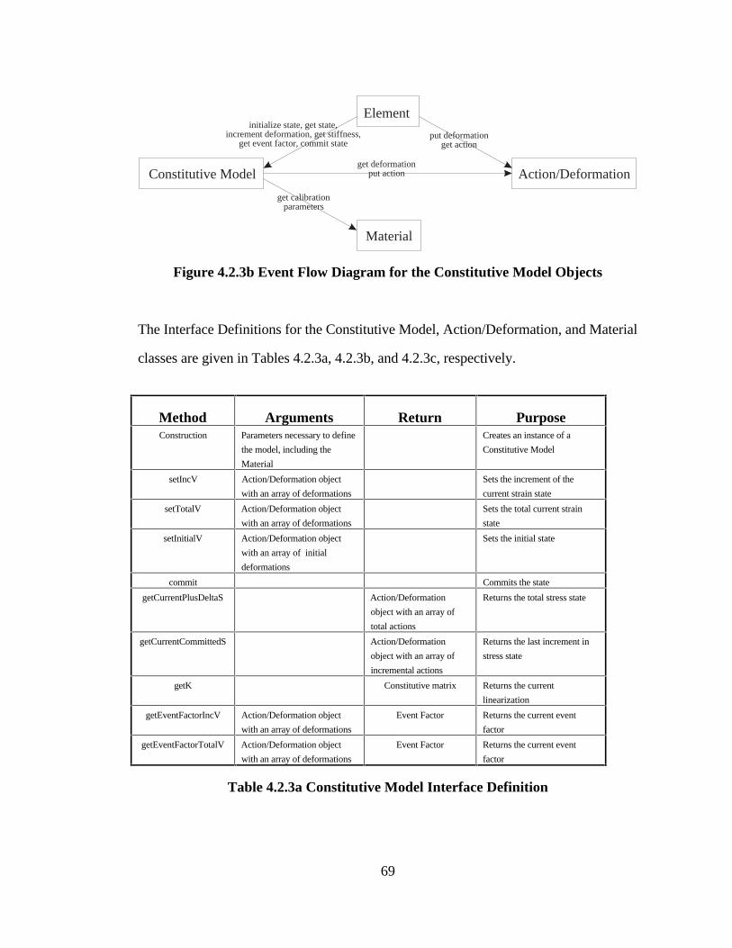
put deformationget action
get calibration parameters
Constitutive Model
initialize state, get state,increment deformation, get stiffness,
get event factor, commit state
Element
Action/Deformation
Material
get deformationput action
Figure 4.2.3b Event Flow Diagram for the Constitutive Model Objects
The Interface Definitions for the Constitutive Model, Action/Deformation, and Material
classes are given in Tables 4.2.3a, 4.2.3b, and 4.2.3c, respectively.
Method Arguments Return PurposeConstruction Parameters necessary to define
the model, including the
Material
Creates an instance of a
Constitutive Model
setIncV Action/Deformation object
with an array of deformations
Sets the increment of the
current strain state
setTotalV Action/Deformation object
with an array of deformations
Sets the total current strain
state
setInitialV Action/Deformation object
with an array of initial
deformations
Sets the initial state
commit Commits the state
getCurrentPlusDeltaS Action/Deformation
object with an array of
total actions
Returns the total stress state
getCurrentCommittedS Action/Deformation
object with an array of
incremental actions
Returns the last increment in
stress state
getK Constitutive matrix Returns the current
linearization
getEventFactorIncV Action/Deformation object
with an array of deformations
Event Factor Returns the current event
factor
getEventFactorTotalV Action/Deformation object
with an array of deformations
Event Factor Returns the current event
factor
Table 4.2.3a Constitutive Model Interface Definition
69

Method Arguments Return PurposeConstruction Creates an instance of a
Action/Deformation
putAction array of actions stores actions
getAction array of actions reports actions
putDeformation array of deformations stores deformations
getDeformation array of deformations reports deformations
Table 4.2.3b Action/Deformation Interface Definition
Method Arguments Return PurposeConstruction Any parameters necessary to
define the material
Creates an instance of a
Material
getYM Young's Modulus Returns the Young's Modulus
getPoison Poison's Ratio Returns the Poison's Ratio
getCompYield Compressive Yield Stress Returns the Compressive Yield
Stress
getTenYield Tensile Yield Stress Returns the Tensile Yield
Stress
Table 4.2.3c Material Interface Definition
4.2.4 Constraint
Collectively, the Constraint objects are responsible for representing the homogeneous
multi-point constraints between the Degree of Freedom Components contained within a
Model. A single Constraint object represents a single equation of constraint. A Degree
of Freedom Component may represent an entire Scalar Degree of Freedom or just one
component of a Vector Degree of Freedom. The processing of these constraints is
accomplished by the Constraint Handler. The Constraint objects collect and report on
the constraints themselves. Symbolically, the constraint equations are in the form of:
C d = 0
where d represents a vector of the degree of freedom components in the Model, 0 is a
vector of zeros, and C is a sparse matrix of constants that represent the relationship
70

between the degree of freedom components. There are more degree of freedom
components than there are equations of constraint. The Constraint objects are held in a
collection by the Model. Additionally, the Constraint object identifies Degree of
Freedom Components that must be retained by the Constraint Handler in the final set of
equations used by the Analysis. This feature is provided to ensure that Degree of
Freedom Components involved in displacement boundary conditions, and other
operations the Analysis handles, are not constrained out by the Constraint Handler.
The Entity Relationship Diagram for the Constraint object is given in Figure 4.2.4a. A
Model has many Constraint objects. A Constraint object relates many Degree of
Freedom Component Descriptions together to form an equation of the constraint
matrix C.
Model
Constraint DofCompDescrelates
Figure 4.2.4a Entity Relationship Diagram for the Constraint Object
The Constraint object is responsible for reporting the equation of constraint it
represents, and its collection of retained Degree of Freedom Components.
The Event Flow Diagram for the Constraint object is given in Figure 4.2.4b. The
Modeler builds an equation of constraint in terms of Degree of Freedom Component
Descriptions and passes them to the Constraint object. The Modeler may also
designate a Degree of Freedom Component to be retained by the Constraint Handler.
71

Once the set of constraints are complete, the Constraint Handler may ask for the
constraint equation and retained Degree of Freedom Components, to produce the initial
mapping between Model Degrees of Freedom and Analysis unknowns.
Constraint
Constraint Handler
Modeler
add an equation of constraint,specify a dof comp. to be retained
get equation of constraint get list of retained dof comp.
Figure 4.2.4b Event Flow Diagram for the Constraint Object
The Interface Definition for the Degree of Freedom Component Description and the
Constraint class is given in Tables 4.2.4a and 4.2.4b respectively.
Method Arguments Return PurposeConstruction type, group, and axis number creates an instance of single
dof description
comparison Single dof description compares with another single
dof desc object
getType dof type returns the type
getGroup dof group returns the group
getDofNum integer returns the axis number
Table 4.2.4a Degree of Freedom Component Description Interface Definition
72

Method Arguments Return PurposeConstruction equation of constraint creates an instance of
Constraint
addRetained dof component specifies a dof component to be
retained
getRow constraint equation returns the equation of
constraint
getRetained list of dof components returns the list of dof
components to be retained
Table 4.2.4b Constraint Interface Definition
4.2.5 Displacement Boundary Condition
A Displacement Boundary Condition object represents a non-homogeneous single point
constraint that will have a value assigned to it in each Load Case by a Prescribed
Displacement object. A single point constraint may instead be represented within the
Constraint object, but this restricts its value to zero for all Load Cases and instances in
time. The Displacement Boundary Conditions are stored directly by the Model. The
related values are stored in the Load Cases. Displacement Boundary Conditions are
not processed by the Constraint Handler. They are handled directly by the Analysis.
The Entity Relationship Diagram for the Displacement Boundary Condition object is
given in Figure 4.2.5a. A Model may have many Displacement Boundary Conditions.
Each Displacement Boundary Condition refers to a Degree of Freedom Component
Description. A Degree of Freedom Component may represent an entire Scalar Degree
of Freedom or one component of a Vector Degree of Freedom.
73

Model
Disp BC Dof Comp Descrefers to
Figure 4.2.5a Entity Relationship Diagram for the Displacement Boundary
Condition Object
The principal responsibility of the Displacement Boundary Condition object is to
indicate to the Analysis, via the Map, which Degree of Freedom Components are to be
assigned a value by the Load Cases.
The Event Flow Diagram for the Displacement Boundary Condition object is given in
Figure 4.2.5b. The only event the object responds to is a request from the Map for the
Degree of Freedom Component Description to which the Displacement Boundary
Condition applies. Map will transform this to an analysis unknown for the Analysis.
Disp BC Mapget Dof Component
Description
Figure 4.2.5b Event Flow Diagram for the Displacement Boundary Condition
Object
The Interface Definition for the Displacement Boundary Condition class is given in
Table 4.2.5.
74

Method Arguments Return PurposeConstruction dof component creates an instance of
Displacement Boundary
Condition
getDofComp dof component returns the affected dof
component
Table 4.2.5 Displacement Boundary Condition Interface Definition
4.2.6 Load Case
A Load Case is responsible for maintaining Load objects, Prescribed Displacements,
and Initial Element States. The Load objects may be either Nodal Loads or Element
Loads. In either case, the load vector is given to the Map object augmented with the
transformations and coordinate systems used to represent the load vector. Nodal loads
may either be related to Scalar or Vector Degrees of Freedom at a Degree of Freedom
Group or Node. Element loads are related to the Element to which they apply, and are
only responsible for providing the Element with the magnitude and type of element
load. The Element itself performs all calculations. A Prescribed Displacement object
provides the time varying value for a Boundary Condition in the Model. Initial Element
States contain the parameters that describe the initial state of a specific instance of a
type of Element. A Load Case object maintains the collections of Loads, Prescribed
Displacements, and Initial Element State objects under its control, and provides access
to these collections to the Analysis object, via the Map.
The Entity Relationship Diagram for the Load Case object is given in Figure 4.2.6a. A
Model may have many Load Cases. A Load Case consists of many Prescribed
Displacements, Loads, and Initial Element States. A Prescribed Displacement defines a
value and a Time Function at a Degree of Freedom Component. A Load may either be
75

a Degree of Freedom Load or an Element Load. A Load defines an associated Time
Function for its values. An Element Load is of a type related to, and applied to, a
specific type of Element ( e.g. Truss Bar Load for a Truss Bar Element). An Initial
Element State is also of a specific type related to, and applied to, a specific type of
Element. A Degree of Freedom Load is either a Scalar or Vector Load depending on
the type of the Degree of Freedom to which it applies. A Vector Load has a Vector
object to represent its value. A Scalar Load is represented by a scalar.
refers to
Dof Desc.
applies to
Element Load
Truss BarLoad
...
definedat
Model
ElementLoad Case
Load
Dof Comp
Time
applies to
Pres. Disp.
refers to
has a
definedat
VectorLoad
ScalarLoad
Vector
Dof Load
InitialElement State
Truss BarState
...
Figure 4.2.6a Entity Relationship Diagram for the Load Case Object
The Load Case object is responsible for maintaining collections of Prescribed
Displacements, Loads, and Initial Element States. The Load Case has a name which
76

identifies it to the Analysis object. The Load Case provides the Analysis object with
access to the collections of the Loads, Prescribed Displacements, and Initial Element
States when requested. The Prescribed Displacement object is responsible for
providing its value (at a specific time value) to the Map object. The Map object
converts the Degree of Freedom Component Description, provided by the Prescribed
Displacement, into an analysis unknown number for the Analysis object. Degree of
Freedom Loads are responsible for providing the Map object with their load vector (for
a specific time value). The load vector must be augmented with the coordinate systems
in which it is defined in order to allow the Map object to transform it to analysis
unknowns for the Analysis object. The Element Load object does not generate the
loads, but simply registers its presence to the appropriate Element. Later, at the
Element's request, the Element Load object supplies the current magnitude and type of
load. The Element calculates the effect of the load and includes the equivalent nodal
loads in its resisting force calculation. Similarly, an Initial Element State registers its
presence to the appropriate Element and provides its data to it when requested. A
Time Function object stores scaling factors and the associated values of time. It uses
these as interpolation points to provide factors for any given value of time.
The Event Flow Diagram for the Load Case object is given in Figure 4.2.6b. The main
program creates and adds Loads, Initial Element States, and Prescribed Displacement
objects to the Load Case. The Analysis object requests access to the collections of
these objects, in the form of iterators, to build the total load for the Load Case.
77

Modeler
Map
Load Case
add a Load, Initial ElemState or Presc. Disp.
get iterators for the collection of Loads,Initial Elem. States or Presc. Disp
Figure 4.2.6b Event Flow Diagram for the Load Case Object
The Event Flow Diagram for the Prescribed Displacement object is given in Figure
4.2.6c. The Map object requests the Degree of Freedom Description that the
Prescribed Displacement refers to, and also the value of the Prescribed Displacement at
a certain value of time. The Prescribed Displacement object requests the time factor
from the Time Function object to which it refers. It will use this as a scaling factor to
be applied to its base value of displacement.
get dof desc.
Time Function
Map
Presc. Disp.
get factor fora time value
get value
Figure 4.2.6c Event Flow Diagram for the Prescribed Displacement Object
The Event Flow Diagram for the Degree of Freedom Load object is given in Figure
4.2.6d. The Map object requests the Degree of Freedom Description and the value of
the load vector. The load vector is augmented with the coordinate systems in which it
is defined. The Degree of Freedom Load object requests the time factor from the Time
78

Function object. It will use this number as a scaling factor to be applied to its base
value of load.
get dof desc.
Time Function
Map
Dof Load
get factor fora time value
get load vector
Figure 4.2.6d Event Flow Diagram for the Degree of Freedom Load Object
The Event Flow Diagram for the Element Load object is given in Figure 4.2.6e. The
Map object requests the establishment of the Element Load at a certain value of time.
The Element Load object requests the time factor from the Time Function object. It
will use this number as a scaling factor to be applied to its base load value. The
Element Load announces its presence to the Element to which it applies. This Element
later requests the defining data of the Element Load object. Since the Element Load
object is defined for a specific type of Element, the protocol for the requesting of data
is unique to the type of Element involved.
register presence
establish load
Time Function
Element
Map
Element Load
get factor fora time value
get data
Figure 4.2.6e Event Flow Diagram for the Element Load Object
79

The Event Flow Diagram for the Initial Element State object is given in Figure 4.2.6f.
A Map object requests the Initial Element State object to perform the initialization.
The Initial Element State registers its presence to the Element to which it applies. This
Element later requests the defining data of the Initial Element State object. Since the
Initial Element State object is defined for a specific type of Element, the protocol for
the requesting of data is unique to the type of Element involved.
set initial state
initialize
Element
Map
Initial Element State
get data
Figure 4.2.6f Event Flow Diagram for the Initial Element State Object
The Interface Definitions for the Load Case, Load, Prescribed Displacement, Initial
Element State, and Time Function objects are given in Tables 4.2.6a-e.
80

Method Arguments Return PurposeConstruction Load case name creates an instance of Load
Case
addLoad Load object adds a Load object
addPresDisp Prescribed Displacement
object
adds a Prescribed
Displacement object
addInitElSt Initial Element State object adds an Initial Element State
object
loadItr Iterator for the Load objects returns the iterator for the
Load objects
presDispItr Iterator for the Prescribed
Displacement objects
returns the iterator for the
Prescribed Displacement
objects
initElStateItr Iterator for the Initial Element
State objects
returns the iterator for the
Initial Element State objects
Table 4.2.6a Load Case Interface Definition
Method Arguments Return PurposeConstruction Time Function, a dof Desc or
Element
creates an instance of Load
(either dof or Element)
getTF time function returns the time function for
the load
getLoad time value load vector augmented with
Coord Systems in which it is
defined
returns the load vector for a
value of time
getDeltaLoad time value load vector augmented with
Coord Systems in which it is
defined
returns the change in the load
vector, for a value of time,
since the last access
Table 4.2.6b Load Interface Definition
81

Method Arguments Return PurposeConstruction Time Function, a dof Desc,
and a value
creates an instance of
Prescribed Displacement
getDof Dof Component Description returns the dof component
description to which the value
applies
getValue value of time displacement value returns the value of
displacement for a given value
of time
getDeltaValue value of time displacement value returns the change in the value
of displacement, for a given
value of time, since the last
access
Table 4.2.6c Prescribed Displacement Interface Definition
Method Arguments Return PurposeConstruction Element, and parameters that
are unique to that type of
element
creates an instance of a specific
type of Initial Element State
initialize announces its presence to the
Element
getData initial element state data returns the initial element state
data
Table 4.2.6d Initial Element State Interface Definition
Method Arguments Return PurposeConstruction ordered pairs of time and value
quantities
creates an instance of Time
Function
getValue value of time scalar value returns the (possibly
interpolated) value for a given
value of time
Table 4.2.6e Time Function Interface Definition
4.3 Handlers
The object design contains three classes of Handlers, which are used by the Analysis to
manage the more complex tasks that are shared between many different types of
82

analysis. These are the Constraint Handler, the Reorder Handler, and the Matrix
Handler. The Constraint Handler manages the processing of the constraints, the
Reorder Handler manages the ordering of the analysis unknowns according to analyst
specified guidelines, and the Matrix Handler is responsible for providing a specified
type of matrix and vector initialized according to the sparsity of the equations.
4.3.1 Constraint Handler
The Constraint Handler is responsible for processing the Constraint objects and
providing the Map object with an initial mapping between the Model degrees of
freedom and the analysis unknowns for the Analysis object. Conventional constraint
handlers such as Transformation, Penalty Function, and Lagrangian Multiplier should
be available, and new handlers can be created as needed by a particular analysis
method.
In the Transformation Constraint Handler, the Constraint matrix C is converted by the
Handler to a transformation matrix that relates all the degrees of freedom to a
constrained set of degrees of freedom. The constrained set of degrees of freedom are
numbered, and this initial mapping between the Model Degrees of Freedom and the
Analysis unknowns is passed to the Map object. These transformations are applied
when transforming element stiffnesses into those needed in the final set of analysis
unknown.
For the Penalty Function Constraint Handler, the initial mapping between the Model
Degrees of Freedom and the analysis unknowns is one-to-one, with no transformation.
83

The constraints are satisfied by the addition of the term CT α C to the stiffness matrix.
The preparation of the α matrix, and the multiplication of the additional term and its
inclusion in the stiffness matrix, is the responsibility of the Analysis object.
For the Lagrangian Multiplier Constraint Handler, the initial mapping between the
Model Degrees of Freedom and the analysis unknowns is one-to-one, with no
transformation, but an additional set of analysis unknowns is set up by the Handler.
These additional analysis unknowns represent the Lagrangian multipliers. The Analysis
object is responsible for adding the constraint matrix to the stiffness matrix to satisfy
the constraints.
The Entity Relationship Diagram for the Constraint Handler objects is given in Figure
4.3.1a. The Constraint Handler is created by the Analysis object and passed to the Map
object. Upon creation, the Constraint Handler queries the Map to determine the
complete list of Degrees of Freedom and obtains the C matrix, and the list of retained
Degree of Freedom Components, from the Constraint object.
initializes
processes
represents
has a
Analysis
Map
Constraint
Model
Constraint Handler
interfaces with
Figure 4.3.1a Entity Relationship Diagram for the Constraint Handler Object
84

The internal workings of the Constraint Handler object differ widely based on the
method of constraint processing. All three methods query the Map to develop a
complete list of the Degrees of Freedom of the Model. The Penalty Function
Constraint Handler then assigns an analysis unknown to each Degree of Freedom and
builds the one-to-one map. The Lagrangian Multiplier Constraint Handler queries the
Constraint object to determine the number of equations of constraint and adds an extra
analysis unknown for each equation of constraint.
The Transformation Constraint Handler obtains the complete constraint matrix from
the Constraint object. For each equation of constraint, the Handler must identify a
degree of freedom to be constrained out of the model. The Handler also requests from
the Constraint object a list of the degree of freedom components that must be retained
in the analysis unknowns. The Handler must ensure that these degree of freedom
components are not selected to be constrained out of the problem.
The Event Flow Diagram for the Constraint Handler objects is given in Figure 4.3.1b.
The Map object requests the initial mapping between the Model Degrees of Freedom
and the Analysis unknowns. The Constraint Handler queries the Model object for the
list of Degree of Freedom Groups. The Constraint Handler then asks for the list of
Degrees of Freedom from each group in turn. Each Degree of Freedom is also asked
to identify its components. The Constraint Handler may also request the Constraint
object to supply its constraint matrix, the number of equations of constraint, and the list
of degrees of freedom that are to be retained.
85

Map
DofGroup
Constraint
Dof
Constraint Handler
get initialmapping
get list ofdofGroups get list
of dof
get C matrix
get list of retained dof
get numberof components
Figure 4.3.1b Event Flow Diagram for the Constraint Handler Object
The Interface Definition for the Constraint Handler class is given in Table 4.3.1.
Method Arguments Return PurposeConstruction Map object Creates an instance of
Constraint Handler
getNumEq integer Returns the number of analysis
unknowns
getMap dof to analysis unknown map Returns the initial dof to
analysis unknown mapping
Table 4.3.1 Constraint Handler Interface Definition
4.3.2 Reorder Handler
The Reorder Handler is responsible for providing the Map object with a re-ordered
mapping between the model degrees of freedom and the analysis unknowns based on
criteria provided by the Analysis object. To accomplish this task, the Reorder Handler
86

requires complete information regarding the Nodes, Elements, Constraints, and
Displacement Boundary Conditions.
The Entity Relationship Diagram for the Reorder Handler objects is given in Figure
4.3.2a. The Reorder Handler is created by the Analysis object and passed to the Map
object. Upon creation, the Reorder Handler queries the Model to determine the
connectivity between the Degrees of Freedom. The Reorder Handler reorders the
mapping between the Model Degrees of Freedom and the Analysis unknown in the
Map object.
reorders
represents
has a
Analysis
Map
Model
Reorder Handler
interfaces with
Figure 4.3.2a Entity Relationship Diagram for the Reorder Handler Object
The internal workings of the Reorder Handler object are unique to the type of
reordering scheme the object represents. In general, the Reorder Handler will obtain
lists of Elements, Nodes, and Displacement Boundary Conditions from the Model
object. Also, it will obtain from the Map object the initial mapping and the constraint
matrix in terms of the initial analysis unknowns.
The Event Flow Diagram for the Reorder Handler object is given in Figure 4.3.2b. The
Map requests the revised mapping of the Model Degrees of Freedom and the Analysis
87

unknowns. The Reorder Handler requests the lists of Elements and Displacement
Boundary Conditions from the Model. From each Element, the Reorder Handler
requests the list of Degree of Freedom Descriptions to which the Element attaches.
From the Displacement Boundary Condition, the Reorder Handler requests the Degree
of Freedom Component with which it is associated. The Degree of Freedom
Descriptions and Components are converted to initial analysis unknowns by the Map.
Also the Map supplies the Reorder Handler with the constraint matrix in terms of initial
analysis unknowns.
Element
Map
DispBC
Model
Reorder Handler
get revisedmapping
get initial eq numfor a Dof Comp
get lists of ElementsDisplacement BCs
get Dof Compget constaint
matrix
get connectingDof Descriptions
Figure 4.3.2b Event Flow Diagram for the Reorder Handler Object
The Interface Definition for the Reorder Handler is given in Table 4.3.2.
88

Method Arguments Return PurposeConstruction Map object, Model object, and
the reordering parameters
unique to the type of
reordering scheme
Creates an instance of
Constraint Handler
getNewOrder list of analysis unknowns Returns the list of analysis
unknowns in the revised order
Table 4.3.2 Reorder Handler Interface Definition
4.3.3 Matrix Handler
The Matrix Handler is responsible for providing matrices and vectors of a specific type,
initialized according to the connectivity of the Model. Each type of matrix and vector
will have its own Matrix Handler class. The choice of Matrix Handler by the Analysis
object defines the type of matrix or vector it will receive.
The Entity Relationship Diagram for the Matrix Handler objects is given in Figure
4.3.3a. The Matrix Handler is created by the Analysis object. Upon creation, the
Matrix Handler queries the Map to determine the connectivity between the analysis
unknowns.
interfaces with
queries
Analysis
Map Matrix Handler
has a
Figure 4.3.3a Entity Relationship Diagram for the Matrix Handler Object
89

The internal workings of the Matrix Handler object are unique to the type of matrix and
vector the object creates. In general, the Matrix Handler will query the Map object to
determine the connectivity of the analysis unknowns. For example, the Matrix Handler
for the column compacted matrix type will need to know the smallest analysis unknown
connected to each analysis unknown to define the column heights for the matrix.
The Event Flow Diagram for the Matrix Handler object is given in Figure 4.3.3b. An
Analysis object will request an initialized matrix or vector from the Handler. It in turn
queries the Map for the analysis unknown connectivity, builds the required object, and
returns it to the Analysis.
get connectivity info
Map
initialize
get matrix or array
Matrix
Analysis
Matrix Handler
Figure 4.3.3b Event Flow Diagram for the Matrix Handler Object
The Interface Definition for the Matrix Handler is given in Table 4.3.3.
Method Arguments Return PurposeConstruction Map object Creates an instance of a
Matrix Handler
setUpMatrix initialized matrix Creates and returns an
initialized matrix
setUpVector initialized vector Creates and returns an
initialized vector
Table 4.3.3 Matrix Handler Interface Definition
90

4.4 Utility Objects
The object design includes several utility objects that are used throughout the design.
These include geometric objects such as Coordinate Systems, Vectors, and Points;
numerical objects such as Matrices; and specialized augmented objects used to transmit
element and load properties from the model to the analysis.
4.4.1 Geometry
The objects in the Geometry module are responsible for providing the means to
represent and manipulate points and geometric vectors in space. The basic component
of the geometry module is the Coordinate System. Coordinate Systems may be one,
two, or three dimensional, polar, spherical, rectangular, etc. However, all Systems
must be able to provide a transformation to and from the unrotated Three-Dimensional
Rectangular System (Global System). Thus, it is possible to transform between any
two Coordinate System objects. Points are created as an array of ordinates in a given
Coordinate System. The position of a point is obtained by providing a Coordinate
System. The Point will give its ordinates as an array with respect to the Coordinate
System. Geometric Vectors are created by giving an array of ordinates in a Coordinate
System that represent the head of the Geometric Vector. The tail is assumed to be at
the origin of the Coordinate System. The position of a Geometric Vector is obtained
by providing the vector with a Coordinate System. The Geometric Vector will give the
ordinates of its head in that System. Vector addition and subtraction is defined, and
Geometric Vectors can be multiplied by a scalar.
91

The Entity Relationship Diagram for the Geometry objects is given in Figure 4.4.1a.
Geometric Vectors and Points are represented as ordinate arrays in a specific
Coordinate System. Coordinate Systems can be 3D Rectangular, 2D Rectangular, etc.
Coordinate System
3D Rect 2D Rect Polar etc...
PointGeometric Vector
represented in represented in
Figure 4.4.1a Entity Relationship Diagram for the Geometry Objects
Externally, Points and Geometric Vectors are responsible for giving their ordinate
arrays in any given Coordinate System. Additionally, Geometric Vectors can be added
and subtracted, and multiplied by a scalar. Coordinate Systems must be able to provide
transformation matrices, which transform ordinate arrays to and from the global
Coordinate System. Additionally, they may provide transformation to and from other
Coordinate System types.
Internally, Geometric Vectors and Points represent their position with respect to the
global Coordinate System. When asked to provide their ordinate array in another
Coordinate System, the transformation matrix from global is requested from that
System.
92

The Event Flow Diagram for the Geometry objects is given in Figure 4.4.1b. The many
users of the Geometry objects, such as a Node to locate a point in space or a Degree of
Freedom to store the state of a response vector, are represented as three dots. The
user will request the ordinate array in a given Coordinate System from a Geometric
Vector or Point. In turn, the Geometric Vector or Point will request from the given
Coordinate System the transformation from the Global System to the given System.
The Geometric Vector or Point will then transform its ordinates to the given System
and respond to the user's request.
get transformationmatrix to or from global
...
Geo Vector Point
Coordinate System
get ordinatearray
get ordinatearray
get transformationmatrix to or from global
Figure 4.4.1b Event Flow Diagram for the Geometry Objects
The Interface Definitions for the Coordinate System, Point, and Geometric Vector
classes are given in Tables 4.4.1a-c.
93

Method Arguments Return PurposeConstruction parameters unique to the
specific System that relate it to
the global system
Creates an instance of a
specific type of Coordinate
System
num_of_axis number of axis Returns the number of axis in
the Coordinate System
trans_to_global transformation matrix Returns the transformation
matrix to convert ordinates in
this system to the Global
trans_from_global transformation matrix Returns the transformation
matrix to convert ordinates in
Global system to this system
Table 4.4.1a Coordinate System Interface Definition
Method Arguments Return PurposeConstruction An array of ordinates and the
associated Coordinate System
Creates an instance of Point
get_rep_in Coordinate System ordinate array Returns the ordinate array of
the Point in the given
Coordinate System
lengthTo Point distance Returns the distance between
the given Point and this Point
Table 4.4.1b Point Interface Definition
Method Arguments Return PurposeConstruction An array of ordinates and the
associated Coordinate System
Creates an instance of
Geometric Vector
get_rep_in Coordinate System ordinate array Returns the ordinate array of
the head of the Geometric
Vector in the given Coordinate
System
add Geometric Vector Geometric Vector Returns vector addition
subtract Geometric Vector Geometric Vector Returns vector subtraction
multiply Scalar Geometric Vector Multiplies a Geometric Vector
by a Scalar
Table 4.4.1c Geometric Vector Interface Definition
94

4.4.2 Numerical Objects
The purpose of the Numerical objects is to provide a minimal set of general and
specialized vectors and matrices. It is not the intention of this dissertation to
investigate high level algebra support. As discussed in Chapter 2, this has been
investigated both by other finite element researchers and numerical analysts. The
intention of the Numerical objects presented in this section is to determine what the
finite element design requires of numerical objects. The selection of an appropriate
library of Numerical objects can then be made rationally, and the implementation of the
finite element program design can be adjusted accordingly. Although commercial
numerical libraries, such as RogueWave, exist, for the sake of furthering research it is
desirable to choose a library that is publicly available. Due to the universal acceptance
of the FORTRAN based LAPACK library [2], a likely candidate is the C++ based
LAPACK++ library [13], but the final decision is deferred for future work.
There are two types of users of the Numerical objects: small-scale and large-scale.
The Map and Model objects are small-scale users. They use the Numerical objects to
form and transmit element and nodal properties. These objects are small, generally full,
possibly symmetric, and possibly contain blocks of zero or identity entries. The
principal operations performed on these objects are addition, subtraction, transposition,
and multiplication. The Analysis object, on the other hand, is a large-scale user. It may
create large Matrix objects with highly specialized sparsities. These may include
symmetric banded, column compacted, upper or lower triangular, general sparse, etc.
In addition to the basic algebraic operations, the Analysis object requires these Matrix
objects to efficiently perform complex numerical operations such as the solution of
linear equations and the eigenvalue problem. To initialize these objects, the Analysis
95

uses the Matrix Handler associated with the type of matrix or vector needed. The
Handler provides the matrix with the initialization data.
The design of the base abstract Matrix and Vector classes includes only the most
fundamental methods common to all matrix and vector types. That is, access to the
individual elements of the objects, addition, subtraction, multiplication, and
transposition. During the actual implementation of the Numerical object hierarchy,
each subclass of these abstract classes will add their own methods as the
implementation demands. For example, the Analysis will require that the large-scale
matrix objects be able to decompose themselves and solve Ax = b.
The Entity Relationship Diagram for the Numerical objects is given in Figure 4.4.2a.
The abstract class Vector is a one dimensional vector that is a Full Vector. This can be
extended to include sparse data types if required. The abstract class Matrix can be a
Full Matrix, or Symmetric Matrix, etc. This also can be expanded, as required by the
implementation, to include a more efficient library of sparse matrix types.
Matrix
Full Symmetric Block Half Banded Column Compacted
Vector
Full
Figure 4.4.2a Entity Relationship Diagram for the Numerical Objects
The Interface Definitions for the Vector and Matrix classes are given in Tables 4.4.2a
and 4.4.2b.
96

Method Arguments Return Purposeelement access element position number Returns the element at a given
position
element insertion number and element position Inserts a number in a given
position
addition Vector Vector Adds two Vectors
subtraction Vector Vector Subtracts one Vector from
another
multiplication Vector, Scalar, or Matrix Vector, or Matrix Multiplies a Vector by another
Vector, Scalar, or Matrix
Table 4.4.2a Vector Interface Definition
Method Arguments Return Purposeelement access element position number Returns the element at a given
position
element insertion number and element position Inserts a number in a given
position
addition Matrix Matrix Adds two Matrices
subtraction Matrix Matrix Subtracts one Matrices from
another
transposition Matrix Returns the transpose of a
Matrix
multiplication Vector, Scalar, or Matrix Vector, or Matrix Multiplies a Matrix by another
Matrix, Scalar, or Vector
Table 4.4.2b Matrix Interface Definition
97

4.4.3 Augmented Vector and Matrix Objects
As described in earlier sections, the Element and Nodal properties are transmitted to
and from the analysis via matrices and vectors that are augmented with pending
transformations. For example, an Element will internally produce its stiffness matrix ke
according to some elemental system known only to itself. To communicate the
stiffness to the Analysis, the Element must generate a transformation matrix Te lT−− that
will transform the Matrix to the local Coordinate Systems at the Nodes. Furthermore,
the Map will add a transformation matrix Tl nT−− to transform the Matrix to the actual
nodal Coordinate Systems, and an additional transformation matrix Tn aT−− to transform
the Matrix appropriately for the Analysis unknowns. Algebraically, this process of
producing Kea, an element stiffness matrix in terms of Analysis unknowns, is
represented as:
K T T T k T T Tea n aT
l nT
e lT
e e l l n n a= − − − − − −
To reduce the number of computations, it is advantageous to combine the pending
transformations into one before performing the matrix triple product.
The Augmented Vector and Augmented Matrix objects contain the original Vector or
Matrix, and a collection of pending Transformation objects. The Transformation
objects consist of a Block Matrix and a collection of Degree of Freedom Descriptions.
The Description objects label the columns of the object that result from the application
of all the pending Transformations. The Augmented Vector and Matrix objects
provide the following public methods: a method to add additional transformations; a
98

method to provide the descriptions for the last transformation added; and a method
which applies the pending transformations and produces the final vector or matrix.
The Block Matrix object is chosen to represent the transformation matrices to take
advantage of the natural block structure that arises from the use of Geometric Vectors
to define the nodal values. The collection of Degree of Freedom Descriptions
associated with the transformation are in terms of complete Vector and Scalar Degrees
of Freedom. Thus, the components of the Geometric Vectors represented in the
columns and rows of the matrices must be contiguous. Therefore, the transformation
matrices will have a natural block structure. For transformations between local and
nodal Coordinate Systems, many of these blocks will be zero. Also, if some of the
local and nodal systems are identical, the associated block will be the identity matrix.
The Block Matrix object is capable of taking advantage of this structure.
The Entity Relationship Diagram for the Augmented Vector and Matrix objects is given
in Figure 4.4.3a. An Augmented Vector has a single Vector object, and an Augmented
Matrix has a single Matrix object. Augmented Vector and Matrix objects have many
Transformations. The Transformations consist of a single Block Matrix object and
many Degree of Freedom Descriptions.
99

Augmented Vector Augmented Matrix
Transformation
Dof Description Block Matrix
Vector Matrix
Figure 4.4.3a Entity Relationship Diagram for the Augmented Vector and Matrix
Objects
Transformations are built up by defining a Block Matrix transformation and, one by
one, the Degree of Freedom Descriptions. Transformations are added to the
Augmented Vector or Matrix object. Transformation objects can pass their collection
of Degree of Freedom Descriptions to the Augmented Vector or Matrix object. The
Augmented Vector or Matrix object can supply the collection of Descriptions of the
last Transformation to be added to the object.
The Event Flow Diagrams for the Augmented Vector or Matrix objects are given in
Figures 4.4.3b-c. The users of the Augmented Vector and Matrix objects are the
Elements and Loads that define the objects, the Map to additionally transform them,
and the Analysis object to request the final transformed objects. Element or Load
object defines the original Matrix or Vector, and adds a Transformation. They create
the Transformations by defining a Block Matrix for the transformation and adding
Degree of Freedom Descriptions. The Map object can retrieve the collection of Degree
of Freedom Descriptions for the last Transformation, and adds additional
Transformations. The Augmented Vector or Matrix requests the list of Degree of
100

Freedom Descriptions from its component Transformations. The Analysis object
requests the final transformed Matrix or Vector.
add a Transformationget last Trans. Desc
define original Vector
add a Desciptiondefine a Block Matrix
Map
Element or Nodal Load
Augmented Vector
Analysis
Transformation
add a Transformation
apply all Transformations
get last Trans. Desc
get Desciptions
add a Desciptiondefine a Block Matrix
Figure 4.4.3b Event Flow Diagram for the Augmented Vector Object
add a Transformationget last Trans. Desc
define original Matrix
add a Desciptiondefine a Block Matrix
Map
Element
Augmented Matrix
Analysis
Transformation
add a Transformation
apply all Transformations
get last Trans. Desc
get Desciptions
add a Desciptiondefine a Block Matrix
Figure 4.4.3c Event Flow Diagram for the Augmented Matrix Object
101

The Interface Definitions for the Augmented Vector, Augmented Matrix,
Transformation, and Transformation Description classes are given in Tables 4.4.3a-d.
Method Arguments Return PurposeConstruction Vector, and Transformation Creates an instance of
Augmented Vector and sets the
initial vector and first
Transformation
addT Transformation Adds an additional
Transformation
getLastT Transformation Gets the last Transformation
getId Vector of integers Gets the Analysis unknowns
getTranformedLoad Vector Applies the Transformations
and returns the transformed
vector
Table 4.4.3a Augmented Vector Interface Definition
Method Arguments Return PurposeConstruction Matrix, and Transformation Creates an instance of
Augmented Matrix, and set the
initial matrix and first
Transformation
addT Transformation Adds an additional
Transformation
getLastT Transformation Gets the last Transformation
getId Matrix of integers Gets the Analysis unknowns
getTransformedK Matrix Applies the Transformations
and returns the transformed
matrix
Table 4.4.3b Augmented Matrix Interface Definition
102

Method Arguments Return PurposeConstruction number of row and column
blocks
Creates an instance of
Transformation
addDesc Transformation Description
and a matrix, or just a
Transformation Description
Adds a Transformation
Description and associated
transformation matrix, or just a
Transformation Description
putT Block Matrix Defines a transformation
matrix
getDescItr list of Dof Descriptions Gets the list of Dof
Descriptions
getTrans block matrix Returns the complete
transformation matrix
nRow integer Gets the number of rows for
the transformation matrix
nCol integer Gets the number of columns
for the transformation matrix
nRowBlock integer Gets the number of blocks
along a row of the
transformation matrix
nColBlock integer Gets the number of blocks
along a column of the
transformation matrix
Table 4.4.3c Transformation Interface Definition
Method Arguments Return PurposeConstruction dof Type, Group, Coordinate
System
Creates an instance of
Transformation Description
getType dof Type Returns the dof Type
getGroup DofGroup Returns the dof Group
getCoOrdSys Coordinate System Returns the Coordinate System
nDof integer Returns the number of axes of
the Coordinate System
Table 4.4.3d Transformation Description Interface Definition
103

5. Behavior of High Level Classes
The object model described in the previous chapter was implemented in the C++
programming language. A description of the public interfaces for the classes of objects
is contained in the Appendix. The names of the classes are consistent with the design
names except that the prefix "Fea" was added to each class name to avoid conflict with
class names in other libraries. The purpose of the implementation is to validate the
object model design and demonstrate that the design can be implemented. Although
care has been taken to ensure a relatively efficient implementation, efficiency is not the
primary objective. Future work in this area should address efficiency.
The primary aim of the implementation of the software design is the definition of the
interfaces for the classes in the design. The interface defines how the methods of the
class can be used, and what they return. The interface describes the behavior of a class,
it does not describe how these tasks are to be accomplished. The details of how each
specific method is implemented can be changed at any time without affecting any other
104

portion of the implementation. The interface, on the other hand, is difficult to change
once it is established.
This chapter describes the behavior of the important high level objects in the design.
The goal is to provide insight into the implementation, without getting into the details.
The classes described in subsection of this chapter are Elements, Constitutive Models,
Constraint Handler, Map, and Analysis. These sections are geared towards giving the
future designer/programmer information on the features of the system, and how to use
them.
A finite element program must grow to accommodate new demands. Common
adaptations include new elements, constitutive models, and analysis algorithms. Since
future programming tasks are likely to occur in these classes, their implementation is
discussed in this chapter. The system design greatly reduces the complexity of these
classes by providing a rich set of services and specifying the precise behavior of the
classes. The specific services the system provides to these objects, and the services
these objects must provide to the system, are presented.
While it is certainly possible to write new Map and Constraint Handler objects, it is
unlikely that these objects will be reimplemented. The descriptions for the Map and
Constraint Handler are provided here to show precisely how the objects were
implemented. Together, they form the heart of the design. It is not necessary to know
how they perform their actions in order to use and add to the program. The
descriptions are provided to give a more thorough understanding of the system
architecture.
105

5.1 Element
The primary responsibilities of an element are to provide the Analysis with the current
linearized stiffness, mass, damping, and resisting force. A specific type of element
object is a subclass of the abstract class Element. All subclasses of Element must share
the same interface as the Element class. This section describes the behavior common to
all Element objects.
5.1.1 Element Geometry
One of the first tasks an element must perform is to determine its geometry, and
establish a set of local coordinate systems it will use in communication with the other
components of the system. This generally involves querying the Nodes to which it
attaches, to obtain the nodal positioning. For example, the following code fragment is
taken from a beam element which attaches to nodeI and nodeJ , and is given a third
point to define its roll angle.
// nodeI and nodeJ are previously defined FeaNode objects// point is a previously defined FeaGeoPoint object// cs is a Fea3DRect object// l is a double
// create a coord sys using nodeI, nodeJ, and pointcs = Fea3DRect(nodeI.getPosition(),nodeJ.getPosition(), point)
// get length between nodeI and nodeJl = (nodeI.getPosition()).lengthTo( nodeJ.getPosition() )
The first line creates a 3D rectangular coordinate system cs using the two Points
obtained from the Nodes, and a third specified Point. The second line calculates the
106

length of the beam by obtaining the points from the Nodes and making use of the
lengthTo method provided by the Point from nodeI .
The Element will also query the Nodes to obtain the current deformed shape. The
Nodes provide the deformations as FeaGeoVectors. The Element uses its local
coordinate systems to interpret the vectors as ordinate arrays. For example, the
following code fragment obtains the increment in translational displacement from
nodeI and interprets it as an array of ordinates in the Element's local coordinate
system localCS .
// nodeI is a previously defined FeaNode object// localCS is a previously defined FeaCoOrdSys object// vec is a FeaGeoVector object// ord is a FeaFullVector object
// get current increment translation disp from nodeIvec = nodeI.getIncV("translation")
// get the ordinates that represent vec in the localCSord = vec.get_rep_in(localCS)
5.1.2 Communication of Element Properties
The properties of the Element are transmitted to the Map via an FeaAugmentedMatrix.
An FeaAugmentedMatrix object holds the basic property matrix and a collection of
pending transformations. The transformations consist of a transformation matrix and a
collection of transformation descriptions which identify the basis of the matrix after the
transformation has been applied. The Element is responsible for providing the basic
property matrix and a transformation that would place the matrix in terms of coordinate
systems recognizable to the Map (i.e. FeaCoordinateSystem objects). For example, the
basic stiffness matrix for a 1D truss bar is a 1x1 matrix k Al= E , which is in terms of
107

Element's internal system of action/deformation measurement. To communicate the
stiffness matrix to the Map, k must be transformed into a complete representation at all
nodes using K a kat= , where a = 1 1− consists of two 1x1 partitions. The code
for this is:
// nodeI and nodeJ are previously defined FeaNode objects// cs is a previously defined Fea1DRect object// t1, t2, and k are 1 by 1 FeaFullMatrix objects
// define the transformation t with 1 by 2 blocksFeaTransformation t(1,2)
// define the first transformation blockt1(0,0) = 1.0t.addDesc(FeaTransDesc("translation", nodeI, cs), t1)
// define the second transformation blockt2(0,0) = -1.0t.addDesc(FeaTransDesc("translation", nodeJ, cs), t2)
// define the basic stiffness AE/lk(0,0) = A*E / l
// create the augmented matrix with k and tFeaAugmentedMatrix(k, t)
The first line forms a FeaTransformation object t in which the transformations have a
block structure of 1 by 2 (matrix a above). The blocks of the a matrix are defined as
t1 and t2 . These are added to t along with a FeaTransDesc object which defines the
block. In this case, the first block refers to a "translation" degree of freedom at
nodeI . The coordinate system cs is a one-dimensional rectangular system defined by
the Element. It lies along the axis of the member and points from nodeI to nodeJ .
The matrix k is then defined, and both k and t are used to form the
FeaAugmentedMatrix object which represents the stiffness of the bar.
108

5.1.3 Element State
One of the principal functions of the Element is the tracking of its state. An Element is
required to keep track of the current-committed state, and an increment from the
current-committed state. Together they form the total state. The properties the
Element reports are always consistent with the total state. An Element state may be
updated through many trial states, through adjustment to the increment in state. When
the analysis is satisfied, the Element state is committed. The committed state becomes
part of the solution path. A commit implies that the committed state must be put into
accord with the total state, and the increment in state is set to zero. A commit defines
a family of possible states for the Element, and an update selects a state in the family.
An event factor is the proportion of the increment in state a component of the Element
can accommodate without violating the assumptions of its linearization.
The Element presents three methods for control of its state. Namely, updateState ,
commit , and getEventFactor . For an updateState , the Element retrieves
the current response quantities at the Nodes to which it attaches, and interprets it to
update its own increment in state. Since the Element may experience many such trial
states, the trial states must be recoverable. A state commit implies that the state the
Element interprets from the Nodes is on the solution path. Thus, the Element may be
inelastic immediately after a commit. The state of the Element must remain unchanged
during an event factor calculation. If an event factor calculation causes the Element to
adjust the state of one of its sub components, it must return it to the previous state
upon completion.
109

In dealing with the Constitutive Models and Nodes, the Element writer must be aware
of these state terms. The Nodes can provide their current committed response
quantities, the increment in the response quantities from the current committed, and the
total. Likewise, the Constitutive Models can be updated by specifying an addition to
the increment in state, or by specifying a new total state, which updates the incremental
state. An Element writer is free to select whichever form is more convenient. If the
Element writer chooses to obtain the total response quantities from the Nodes, it is
likely that the Constitutive Model will be updated by specifying a new total state in
deformation. Whereas if the Element writer obtains the increment in response
quantities from the Nodes, adding to the increment of the Constitutive Model would
likely be more convenient. In either case, only the increment in state is modified; the
committed state remains unchanged.
5.1.4 Action/Deformation
Constitutive Model objects are used by the Element to provide the relationship
between, and track the state of, action and deformation within the Element. The
Element must use a specific type of Action/Deformation object in its communication
with the Constitutive Model object. For example, all the Constitutive Models for a
moment-rotation Constitutive Model (FeaMRLinearElastic, FeaMRElasticPlastic, etc.) use
a moment-rotation Action/Deformation object. Each Action/Deformation object has its
own methods to get and set the action and deformation. For instance, the following
code creates a FeaMRActDef object ad , sets the rotation to 0.001, and uses it to update
the state of a FeaMRElasticPlastic object cm
110

// cm is a previously defined moment/rotation (MR) constitutivemodel
FeaMRActDef ad // define the MR action/deformation objectad.setR(0.001) // set the rotation to 0.001cm.setTotalV(ad) // update state of cm to a rotation of 0.001
Likewise the current committed moment value is obtained as:
// cm is a previously defined MR constitutive model// ad is a FeaMRActDef object// moment is a double
ad = cm.getCurrentCommittedS() // get the act/defmoment = ad.getM() // get the moment
The getCurrentCommittedS method of cm returns a FeaMRActDef object, which
in turn is sent the message getM .
5.1.5 Resisting Force
Another basic premise of the system design is that the Element resisting force
calculation includes the effect of all element loads and initial states. In other words,
element loads and initial states only are included in the equilibrium equations through
the elements. This allows the distribution of the forces to be modified according to the
non-linear inelastic behavior of the Element. For example, if a hinge were to develop in
a beam element during analysis, the internal distribution of element loads could be
adjusted accordingly.
5.2 Constitutive Model
A Constitutive Model object defines the nature of the relationship between measures of
action and deformation (such as stress and strain). These measures are defined by
111

Action/Deformation objects. The Material object provides data for the Constitutive
Model. For example, a Constitutive Model might be one-dimensional-elastic-perfectly-
plastic, the Action/Deformation object would be 1D-stress-strain, and a Material could
be A36-steel. The Material object would provide the modulus of elasticity and the yield
stress to the Constitutive Model object. An Element may be composed of many
Constitutive Model objects. A Constitutive Model can initialize, update, commit, and
report on its state at the request of an Element. It maintains the last committed state,
and the increment from it to the current state. In accordance with the object design, the
Constitutive Model must remain elastic during an update of its state, but may be
inelastic immediately after its state is committed.
5.2.1 Material Data
The intention of the system design is that a Constitutive Model object obtain its data
from a Material object. This concept works well for the typical solid modeling
elements that require the Constitutive Models to communicate the Action/Deformation
in terms of stress and strain. In these cases, the Constitutive Model needs only a
Material object to provide the material properties. For example, the following code
fragment would be appropriate as the constructor for a 2D elastic plane stress
Constitutive Model. The Material object supplies all the necessary information to
instantiate the class; namely Poisson's Ratio and Young's Modulus.
112

Fea2DElasticPlaneStress(FeaMaterial mat)// constructor for 2D elastic plane stress constitutive model// mu and e are instance variables of the class{
...
mu = mat.poisson(); // set Poisson's Ratioe = mat.youngsModulus(); // set Young's Modulus
...}
For Constitutive Models with more complex measures of action and deformation, more
information must be specified to the Constitutive Model. For example, a Constitutive
Model that relates moment to rotation may need both the Material and the moment of
inertia of the section. The Material's Young's Modulus is obtained and combined with
the given moment of inertia for the section to produce the bending stiffness.
FeaMRLinearElastic(FeaMaterial mat, double i)// constructor for Moment Rotation linear elastic constitutivemodel// EI is an instance variable for the class{
...
EI = mat.youngsModulus() * i; // bending stiffness
...}
5.2.2 Action/Deformation
Constitutive Models are subclassed according to their measures of action and
deformation. Elements can select the abstract class for the Constitutive Model based
on the desired measure of action and deformation. This allows Elements to be
programmed without reference to a specific Constitutive Model. Any subclass of the
abstract Constitutive Model can be used since the subclass must also use the same
113

measures of action and deformation. For example, a beam element with hinges may
use a moment-rotation type of Constitutive Model for its hinges. This dictates that the
communication between the Element and Constitutive Model will be performed by
using a FeaMRActDef object. Any subclass of the FeaMRConstitutiveModel class, such as
FeaMRLinearElastic or FeaMRElasticPlastic, can be used. The implication of this is that
the author of a new subclass of FeaConstitutiveModel must also create a subclass of
FeaActDef. For example, the FeaMRConstitutiveModel class works with the
FeaMRActDef class. The interface for the FeaMRActDef is given below. The method
implementations are inlined for both efficiency and to show the simplicity of the
implementation.
// interface for the FeaMRActDef class// subclass of the FeaActDef class
class FeaMRActDef : public FeaActDef{// private instance variablesdouble moment; // moment valuedouble rotation; // rotation value
public:// constructorFeaMRActDef() { moment = rotation = 0.0; };
// get and set the momentdouble getM() { return moment };setM(double m) { moment = m; };
// get and set the rotationdouble getR() { return rotation };setR(double r) { rotation = r; };
};
The Constitutive Model uses its Action/Deformation class in virtually all its
communication with the Element. The exception to this is for the transfer of the
constitutive matrix which uses an FeaMatrix. A Constitutive Model will generally
obtain the deformation measures the Element provides, and set the action measure the
Element demands. For example, the following code fragment is taken from the last
114
lines of a request, from the element, for the current moment. A FeaMRActDef object ad
is created. The value of the currentM , calculated previously by the method, is used
to set the moment in ad . Finally, the action/deformation object is then returned to the
Element.
// currentM is a previously defined variableFeaMRActDef ad // define the MR action/deformation objectad.setM(currentM) // set the moment to currentMreturn (ad) // return the act/def object to the element
Likewise, an Element specifies a change in state by providing an action/deformation
object containing deformation data. In the following code fragment, the rotation is
obtained by a Constitutive Model from a FeaMRActDef object ad , provided by an
Element, as:
// ad is a FeaMRActDef object// rotation is a double
rotation = ad.getR() // get the rotation from ad
5.2.3 Constitutive Model State
One of the principal functions of the Constitutive Model is the tracking of its state. An
Constitutive Model is required to keep track of the current-committed state, and an
increment from the current-committed state. Together they form the total state. The
semantics of these state terms are the same as for Elements described previously.
The Constitutive Model presents five methods for control of its state. Namely;
setIncV , setTotalV , commit , getEventFactorIncV , and
getEventFactorTotalV . The trial state of a Constitutive Model is updated by an
Element using either the setIncV (to specify a new increment in deformation) or
115

setTotalV (to specify a new total deformation) methods. In both cases the
Element passes the deformation data, in the argument list for the method, as an
action/deformation object. Since the Constitutive Model may experience many such
trial states, the trial states must be recoverable. A commit implies that the state of the
Constitutive Model is on the solution path. For a commit, the Constitutive Model sets
the current-committed state to the total state, and zeros the increment in state. A
Constitutive Model may be inelastic immediately after a commit.
To obtain an event factor, the Element must provide the Constitutive Model with a
temporary trial state which is discarded by the Constitutive Model at the end of the
event factor calculation. The state of the Constitutive Model must not be changed by
an event factor calculation. The event factor is obtained by an Element using either the
getEventFactorIncV (to specify a new temporary increment in deformation) or
getEventFactorTotalV (to specify a new temporary total deformation)
methods. In both cases the Element passes the deformation data, in the argument list
for the method, as an action/deformation object.
5.3 Analysis
The responsibility of the Analysis objects (FeaAnalysis) is to collect the various
properties of a Model, including the initial conditions and loading, perform the analysis,
and post the appropriate response quantities to the Model. Analysis objects deal only
with analysis unknowns. They have no knowledge of nodes or degrees of freedom.
Thus element and nodal properties are transmitted to the Analysis objects, and results
are passed back from the Analysis objects in terms of these unknowns. The Analysis
116

object interacts with the Map object, and generally has no direct access to the Model.
An Analysis object does not process the homogeneous multi-point constraints; these
are handled by the Constraint Handler. It does, however, have to consider the non-
homogeneous single point displacement boundary conditions.
This section describes the facilities of the program that the Analysis objects will use to
accomplish the analysis tasks; namely, the Map, the Constraint Handler, the Reorder
Handler, and the Matrix Handler. Also, since the Analysis objects must take care of the
boundary conditions and prescribed displacements, a description of one method for
dealing with these is given, along with implementation examples.
5.3.1 Analysis Constructors
The constructor for each Analysis class creates a Constraint Handler, a Reorder
Handler, a Map, and a Matrix Handler to aid in the analysis. It may also initialize the
various property matrices and vectors, such as the stiffness matrix and resisting force
vector. The order of creation for the handlers is important. The Constraint Handler
and Reorder Handlers must be created first. Next, the Map is created using the
Constraint and Reorder Handlers in the argument list. Finally, the Matrix Handler is
constructed using the Map. The Matrix Handler is then used to provide initialized
matrix and vector objects for the Analysis. The implementation for a typical analysis
constructor is shown below.
FeaTypicalAnalysis(FeaModel model)// a typical constructor for an analysis class
// instance variables// sub model
117

// conH constraint handler// reoH reorder handler// m map// matH matrix handler// k stiffness matrix// rf resisting force vector{
// save the model to be analyzedsub = model;
// create the constraint handler (transformation method)conH = new FeaTransConHandler(sub);
// create the reordering handler (no reordering)reoH = new FeaNoOrderHandler(sub);
// create the FeaMapm = new FeaMap(sub, conH, reoH);
// create the matrix handler (column compacted)matH = new FeaColCompMatrixHandler(m);
// form the instance variablesk = matH.setupMatrix(); // stiffness matrixrf = matH.setupVector(); // resisting force vector
}
Although the actual construction of the Handler objects is trivial, the choice of subclass
for each Handler dictates much about the Analysis. The FeaTransConHandler uses the
transformation method to process the constraints. As such, the Analysis object needs
to do nothing else with the constraints other than construct the handler. If the chosen
Handler uses the method of penalty functions or Lagrangian multipliers (or some other
Handler subclass), the Analysis object must perform some additional tasks during the
analysis procedure. For the method of penalty functions, the Analysis must include the
CT α C in the stiffness matrix. The preparation of the α matrix, and the multiplication
of the additional term and its inclusion in the stiffness matrix, is the responsibility of the
Analysis object. For the method of Lagrangian multipliers, an additional set of analysis
unknowns is added to the Map. These additional unknowns represent the Lagrangian
multipliers. The Analysis object is responsible for adding the constraint matrix to the
118

stiffness matrix to satisfy the constraints. Some Reorder Handlers are intended for use
with a specific type of constraint handler. Use with other types of Constraint Handlers
may result in inefficient equation ordering schemes. Thus, care must be taken in the
Reorder Handler selection. The choice of subclass used for the Matrix Handler dictates
the storage scheme and solver algorithms available for the matrices it creates. This may
greatly affect the performance of the Analysis.
5.3.2 Analysis State
The Analysis object uses the Map to manage the state of the Model. Through the Map,
the state of the Model can be updated, committed, and reported. The components of
the Model are required to keep track of the current-committed state, and an increment
from the current-committed state. Together they form the total state. For an iterative
solution procedure, each iteration adds to or subtracts from (updates) the increment in
the state of the Model. These trial states are not part of the solution path. When the
Analysis is satisfied, the state of the Model is committed. The committed state
becomes part of the solution path. A commit implies that the committed state must be
put into accord with the total state, and the increment in state is set to zero. A commit
defines a family of possible states for the Model, and an update selects a state in the
family. An event factor is the proportion of the increment in response a component of
the Model can accommodate without violating the assumptions of its linearization. The
state of the Model remains unchanged during an event factor calculation.
The Map provides several methods for state update. The Nodes of the Model are
updated by the Map by passing a new increment in response or total response (or time
119

derivative), to the updateDofGroupsByInc and updateDofGroupsByTotal
methods respectively. The Map's updateElements method updates the state of all
Elements in the Model. When the Analysis is satisfied with the state, the Model can be
committed. The commit method of Map will commit the state of all Elements and
Nodes in the Model. The minimum event factor from the elements is obtained through
the Map's getMinEventFactor method. The Map's scaleBy method scales the
increment in response at the Nodes by a given factor, usually the value returned by the
Map's getMinEventFactor method.
5.3.3 Assembly
The properties of the Model, such as stiffness, mass, damping, resisting force, and
applied load, are obtained through the Map via FeaAugmentedMatrix and
FeaAugmentedVector objects. These objects contain the basic property matrix or vector
and transformations that will put the property in an analysis unknown basis. Matrix and
vector objects have an assemble method which takes a FeaAugmentedMatrix or
FeaAugmentedVector object, requests the application of the pending transformations and
analysis unknown identification, and assembles the results. For example, a
FeaAugmentedMatrix object kel , representing an Element stiffness matrix, can be
assembled into the system stiffness matrix k using:
// k is the model stiffness matrix (FeaMatrix)// kel is an element stiffness matrix (FeaAugmentedMatrix)k.assemble( kel );
The Map object provides the Analysis with iterators for the appropriate components of
the Model that the Analysis must access directly. These are the Elements, Boundary
Conditions, Loads, and Prescribed Displacements. Extending the above example, the
120
Analysis can assemble the stiffness for the entire Model by first obtaining the iterator
for the Elements from the Map. Iterating through each Element, the Analysis then
obtains the FeaAugmentedMatrix representing the stiffness of the Element. Each
Element's stiffness is transformed and assembled into the overall model stiffness matrix.
The implementation for this is:
// m is the map object// k is the model stiffness matrix (FeaMatrix)// iterate thru the Elements
elementItr = m.elementItr(); // get the element iteratoriterateThrough (elementItr){
// get the augmented element stiffness matrixkel = m.getElStiff( elementItr() );
// assemble the transformed element stiffnessk.assemble( kel );
}
5.3.4 Treatment of Boundary Conditions
Analysis objects are responsible for the inclusion of Boundary Conditions and
Prescribed Displacements in the Analysis. One such method for dealing with these
single point constraints is by adding a large stiffness value at the appropriate
equilibrium equation, and increasing the corresponding applied load to produce the
correct displacement value. This will affect the manner with which the Analysis object
assembles the stiffness, applied load, and resisting force of the Model. The
implementation for this is shown below.
void assembleK()// assembles the stiffness matrix k// and adds a large spring to account for the boundary conditions// m is the map for the model// m and k are assumed to be instance variables for the class{
121

// iterate thru the ElementselementItr = m.elementItr(); // get the element iteratoriterateThrough (elementItr){
// get the augmented element stiffness matrixkel = m.getElStiff( elementItr() );
// assemble the transformed element stiffnessk.assemble( kel );
}
// iterate thru the boundary conditions and add a stiff springbcItr = m.bCItr(); // get the boundary condition iteratoriterateThrough (bcItr){
// add a large spring on the diagonal of kk(bcItr(),bcItr()) += LARGE_SPRING;
}}
void assembleLoad()// assembles the load vector p// and increases the loads to account for the prescribed disp// m is the map for the model// m and p are assumed to be instance variables for the class{
// assemble the loadsloadItr = m->loadItr(lc); // get the load iteratorfor ( loadItr.init(); ! loadItr; ++loadItr ){
// get the augmented load vectorldv = m.getLoad( loadItr() );
// assemble the transformed load into pp.assemble( ldv );
}
// process prescribed displacementspdItr = m.presDispItr(lc); // get the prescribed disp iteratorfor ( pdItr.init(); ! pdItr; pdItr++ ){
// get the affected equation number and value from mapeq = m.getEqPD(pdItr());val = m.getValuePD(pdItr());
// add a large force to p that will produce the dispp(eq) += LARGE_SPRING * val;
}}
void assembleLoad(double time)// assembles the load vector p
122

// and increases the loads to account for the prescribed disp// m is the map for the model// m and p are assumed to be instance variables for the class{
// assemble the loadsloadItr = m->loadItr(lc); // get the load iteratorfor ( loadItr.init(); ! loadItr; ++loadItr ){
// get the augmented load vectorldv = m.getLoad( loadItr(), time );
// assemble the transformed load into pp.assemble( ldv );
}
// process prescribed displacementspdItr = m.presDispItr(lc); // get the prescribed disp iteratorfor ( pdItr.init(); ! pdItr; pdItr++ ){
// get the affected equation number and value from mapeq = m.getEqPD(pdItr());val = m.getValuePD(pdItr(), time);
// add a large force to p that will produce the dispp(eq) += LARGE_SPRING * val;
}}
void assembleResForce()// assembles the resisting force vector rf// and accounts for the reaction force at the boundary conditions// m is the map for the model// m and rf are assumed to be instance variables for the class{
// assemble the element resisting forceselementItr = m.elementItr(); // get the element iteratorfor ( elementItr.init(); ! elementItr; elementItr++ ){
// get the augmented force vectorldv = m.getResistingForce( elementItr() );
// assemble the transformed force into rfrf.assemble( ldv );
}
// process boundary conditionsbcItr = m.bCItr(); // get the boundary condition iterator
123

for ( bcItr.init(); ! bcItr; bcItr++ ){
// add the reaction force into rfrf(bcItr()) += LARGE_SPRING * d(bcItr());
}}
5.4 Constraint Handler
The Constraint Handler is responsible for processing the homogeneous multi-point
constraints and providing the Map object with an initial mapping between the model
degrees of freedom and the unknowns in the Analysis object. The system would supply
a variety of common handlers for constraints, such as Transformation, Penalty
Function, or Lagrangian Multiplier. New handlers can be added as needed and used in
new analysis methods.
This section describes the theory and behavior of an implemented Constraint Handler
using the transformation method; namely the FeaTransConHandler. It is not likely that
this class will be re-implemented in the future. The description provides an
understanding of the behavior of the Constraint Handler.
5.4.1 Transformation Theory
The primary objective of the FeaTransConHandler is to produce a transformation matrix
T, based on the equations of constraint C, that transform the degrees of freedom D to
the analysis unknowns. The transformation is the initial mapping that is given to the
Map object. To produce this transformation, the FeaTransConHandler object must
select the degrees of freedom to be retained (Dr) and those to be condensed out (Dc).
124

The modeler can also specify degrees of freedom that are to be retained by the
Constraint Handler. The constraint matrix and degree of freedom vector are
partitioned accordingly, thus the equation of constraints is:
C CD
Dr c
r
c
= L
NM
O
QP 0
Assuming independent constraints, there will be as many degrees of freedom condensed
out as there are equations of constraint. In this case, Cc will be a square matrix. Dc
must be chosen to ensure that Cc is nonsingular. Multiplying out the terms and
rearranging gives:
D C D
C C C
c rc r
rc c r
=
where
= - −1
Thus the transformation matrix T is given as:
D
DT D
TI
C
r
cr
rc
L
NM
O
QP
L
NM
O
QP
=
where
=
There is a one-to-one correspondence between the retained degrees of freedom Dr and
the analysis unknowns. Therefor, T is the transformation between the complete set of
125

degrees of freedom and the analysis unknown. The reader is directed to Cook et al
[11] for further treatment on the processing of constraints.
The equations of constraint do not refer to all the degrees of freedom in the model.
Many of the degrees of freedom in Cr will not be explicitly represented in the
constraints. The implicit columns of Cr associated with these degrees of freedom will
be zero. Thus, the associated column of Crc will also be zero.
5.4.2 Selection of Analysis Unknowns
The choice of which degrees of freedom are to be constrained out of the problem and
which will become analysis unknowns may affect the rank of Cc and its ability to be
inverted. Clearly none of the degrees of freedom on the list of retained degrees of
freedom may be selected. But the choice of others is at the discretion of the Constraint
Handler. Robinson [32] presents a "rank technique" for the automatic selection of
redundants in the equilibrium equations for the flexibility method of structural analysis,
which is applicable. For each row in C, a pivot is selected from a column not used
previously for pivoting. The Jordan elimination procedure is used to set the pivot to
unity and zero out the remainder of the column. The columns selected for the pivots
define the columns of Cc, and consequently the degrees of freedom to be constrained
out of the problem. Robinson suggests that the pivots can be selected as the largest
absolute entry (whose column has not yet been used for pivoting) for the row either:
1) in the original C matrix before the Jordan elimination procedure has commenced; or
2) in the modified C matrix as the Jordan elimination is applied row by row. Both pivot
selection methods can be foiled by pathological example, but seem to work reasonably
126

well for physically derived constraints. The former strategy was implemented. Further
research in this area is warranted.
For each equation of constraint, the degree of freedom with the largest coefficient is
found. If it has not already been selected, and if it is not on the list of retained degrees
of freedom, it is selected for Cc. Otherwise, the next largest entry that meets that
criteria is chosen.
5.4.3 Data Types
In order to build the transformation matrix, the equations of constraint must be
obtained from the model and stored in a convenient format to allow Cc, Cr, and Crc to
be formed. The constraint matrix will likely reference many more FeaDofCompDesc
objects than equations of constraint. Access to the correct FeaDofCompDesc must be
fast, so a hash table is used. A hash function cHF is provided for the FeaDofCompDesc.
It folds the string representing the type and the pointer to the FeaDofGroup into a single
integer value. Each column of the constraint matrix associated with the
FeaDofCompDesc consists of pairs of equation numbers and the associated coefficient
values. The columns will be sparse since a particular degree of freedom component
will likely only be involved in a few equations of constraint. Thus, a dictionary
representation is used for the columns. The C++ definition of the data type for the
hash table is:
table< FeaDofCompDesc &, dictionary<int, double> >
127

The Constraint Handler must provide the Map object with a mapping between the
degree of freedom components in the Model and the unknowns in the Analysis. The
format for the mapping is defined by the Map object and is detailed in the next section.
The same data type used for the constraint matrix above is used to transmit this
mapping.
5.4.4 Implementation
The implementation for the FeaTransConHandler class is shown below. The interface
for the class is given, followed by the implementations of the methods. Virtually all the
work is performed in the constructor. That is, the constructor forms the mapping
between the degrees of freedom in the Model and the initial unknowns for the Analysis.
The general outline for the constructor method is:
• add all the possible dof to the map m
• get the constraint matrix c and complete list of retained dof
• iterate through the dof in the map, if dof not in c , then make it an equation
• choose dof to be removed and pick the dof with the largest value on the
diagonal of the resulting cc matrix
• generate a cc matrix
• generate each column of cr , find crc , and add to mapping
The mapping can be requested by the FeaMap object by means of the getMap method.
The implementation for the hash function for the FeaDofCompDesc object is also given.
class FeaTransConHandler : public FeaConstraintHandler{// mapping between dof and equationstable< FeaDofCompDesc &, dictionary<int, double> > m;FeaModel* sub; // model to be analyzed
128
int numEq; // number of equationspublic:
// constructorFeaTransConHandler(int nBuckets, FeaModel& sub);
// returns the mappingtable< FeaDofCompDesc &, dictionary<int, double> >& getMap();
};
FeaTransConHandler(int nBuckets, FeaModel& s) : m(nBuckets,cHF)// constructor for the FeaTransConHandler class{
sub = &s;numEq = 0;
// add all the possible dof to the map m
// get the iterator for the list of nodes from the model// and iterateitr = sub.dofGroupItr();iterateThrough ( itr ){
// get the list of dof desc from the node and iterate thruit
itr1 = itr().getDescItr();iterateThrough ( itr1 ){
// loop through the components of the dof and add to mfor ( i = 0; i < itr1().nDof(); i++ ){
// add the component of dof to map mm[ FeaDofCompDesc(itr1().getType(), itr(), i+1) ];
}}
}
// get the constraint matrix c and complete list of retaineddof
// set up the temporary variables c and retainedListtable< FeaDofCompDesc &, dictionary<int, double> > c(10,cHF);doubleEndedList<FeaDofCompDesc&> retainedList;int nRow = 0;
// get the iterator for the constraints from the model// and iterate through ititrcon = sub.constraintItr();iterateThrough ( itrcon ){
// get the iterator for the list of retained dof for this// constraint object and iterate through it, adding to
129

// the list of retained dofiterateThrough ( itrret ){
retainedList.addToEnd(itrret());}nRow++;
// get the iterator for the dictionary describing the row of// constraints and iterate through ititrrow = itrcon().getRowItr();iterateThrough ( itrrow ){
// add row into c matrix// key = FeaDofCompDesc// value = doublec[itrrow().key()][nRow] = itrrow().value();
}}
// iterate thru the dof in the map, if dof not in c then// make it an equationitr2 = m.getItr();iterateThrough ( itr2 ){
if ( ! c.includesKey(itr2().key()) ) // dof not in c{
numEq++;m[itr2().key()][numEq] = 1.0; // add to mapping
}}
// determine the retained dofs
// define the list of dof to be constrained outdoubleEndedList<FeaDofCompDesc&> constrainedList;
// choose dof to be removed (make sure they are not on the // retained list) and pick the dof with the largest value// on the diagonal of the resulting cc matrixfor ( int i = 1; i < nRow+1; i++ ){
FeaDofCompDesc* maxCol = 0;double maxVal = 0.0;// get the iterator for the constraint matrix and iterate// through ititr1 = c.getItr();iterateThrough ( itr1 ){
// make sure the dof has a value in the row,// is not on the retained list and has not already// been chosenif ( itr1().value().includesKey(i) &&
130

(!retainedList.includes(itr1().key())) &&(!constrainedList.includes(itr1().key())) )
{if ( maxVal <= fabs( (itr1().value())[i] ) ){
maxVal = fabs( (itr1().value())[i] );maxCol = &(itr1().key());
}}
}
// add the chosen dof to the list of dof to be constrainedout
constrainedList.addToEnd(*maxCol);}
// generate a cc matrix (unsymmetric)FeaFullMatrix cc(nRow,nRow);int col = 1;
// get the iterator for the constrained dof list and iterate// through it to build cc from citr1 = constrainedList.getItr();iterateThrough ( itr1 ){
// loop thru the possible rows in ccfor ( int row = 1; row < nRow+1; row++ ){
// check if dof in c includes the row of ccif ( c[itr1()].includesKey(row) )
// if so, add the constraint info to cccc(row-1,col-1) = c[itr1()][row];
}col++;
}
// decompose the cc matrixcc.luDecomp();
// generate each column of cr, find crc, and add to mapping
// get the iterator for the constraints c and iterate// through the dofitr4 = c.getItr();iterateThrough ( itr4 ){
// ignore the constrained out dofif ( ! constrainedList.includes(itr4().key()) ){
// fill in column of crFeaFullVector cr(nRow);for ( int i = 1; i < nRow+1; i++ )
131

{if ( itr4().value().includesKey(i) )
cr(i-1) = (itr4().value())[i];}
// solve for crc (store in cr)cc.luForBack(cr);
// fill in the mapping
numEq++;// fill in identity value for this equation numberm[itr4().key()][numEq] = 1.0;
// fill in crc values for constrained out FeaDofint count = 0;
// get the iterator for the constrained dof and iterate// through ititr5 = constrainedList.getItr();iterateThrough ( itr5 ){
m[itr5()][numEq] = -cr(count); // add to the mappingcount++;
}}
}}
table< FeaDofCompDesc &, dictionary<int, double> >& getMap()// returns the dof to equation mapping generated in theconstructor{
return m;}
unsigned int cHF(FeaDofCompDesc & arg)// hash function for the dof component{
// get the name of the node the dof belongs tochar* str = arg.getGroup().getName();int i = strlen(str);int hashval = 0;
// fold the stringwhile ( i > 0 )
hashval += str[--i];
// return the folded valuereturn hashval;
}
132

5.5 Map
The Map object (FeaMap) provides the principal link between the Model and the
Analysis. It is a mapping between the degrees of freedom in the Model and the
unknowns in the Analysis. All communication with the Analysis is in terms of analysis
unknowns, and all communication with the Model and its sub-components is in terms
of degrees of freedom. Although the FeaMap object manages this mapping, it does not
create the information. The mapping is created by the Constraint Handler and
renumbered by the Reordering Handler. At the direction of the Analysis object, Map
obtains the structural property matrices and vectors from the components of the Model,
transforms them as needed to analysis unknowns, and passes them to Analysis. Map
also receives the result vectors from Analysis and distributes them to the Nodes.
This section describes the theory and behavior of the implemented FeaMap. It is not
likely that this class will be re-implemented in the future. The description is provided
to give a more thorough understanding of the system architecture.
5.5.1 Example
The Map object is fairly complicated. The best introduction to its function is by
example. The sample structure shown in Figure 5.5.1a will be used for this purpose.
The example is used to show how model properties, in this case an element stiffness
matrix, are transformed by the Map and given to the Analysis, and how the Map
distributes the results of the Analysis to the Model. These two types of operations are
133
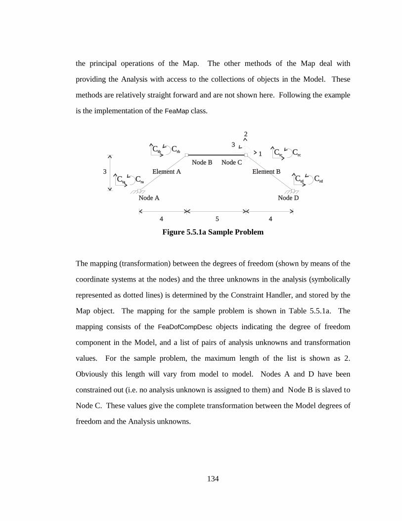
the principal operations of the Map. The other methods of the Map deal with
providing the Analysis with access to the collections of objects in the Model. These
methods are relatively straight forward and are not shown here. Following the example
is the implementation of the FeaMap class.
Cta CraCtd Crd
Ctc Crc
Node A
4 5 4
Element A3
Node D
Node CNode BElement B
2
31
Ctb Crb
Figure 5.5.1a Sample Problem
The mapping (transformation) between the degrees of freedom (shown by means of the
coordinate systems at the nodes) and the three unknowns in the analysis (symbolically
represented as dotted lines) is determined by the Constraint Handler, and stored by the
Map object. The mapping for the sample problem is shown in Table 5.5.1a. The
mapping consists of the FeaDofCompDesc objects indicating the degree of freedom
component in the Model, and a list of pairs of analysis unknowns and transformation
values. For the sample problem, the maximum length of the list is shown as 2.
Obviously this length will vary from model to model. Nodes A and D have been
constrained out (i.e. no analysis unknown is assigned to them) and Node B is slaved to
Node C. These values give the complete transformation between the Model degrees of
freedom and the Analysis unknowns.
134

Dof Description Constraint Transformation Information
Node Dof Type Axis Unknown Factor Unknown Factor
A translation 1A translation 2A rotation 1B translation 1 1 1.0B translation 2 2 1.0 3 -5.0B rotation 1 3 1.0C translation 1 1 1.0C translation 2 2 1.0C rotation 1 3 1.0D translation 1D translation 2D rotation 1
Table 5.5.1a Mapping of Degrees of Freedom to Analysis Unknowns
5.5.1.1 Transformation of a Stiffness Matrix
To demonstrate the use of this mapping, consider the case of the transformation of the
stiffness matrix for Element A. Element A will internally produce its stiffness matrix ke
according to the elemental system. It also generates a transformation matrix Te l− that
will transform the matrix to be in terms of local coordinate systems at the Nodes. The
Map defines a transformation matrix Tl n− to put the matrix in terms of the actual nodal
coordinate systems that describe the degrees of freedom, and an additional
transformation matrix Tn a− to put the matrix in terms of the analysis unknowns.
Algebraically, this process of producing Kea, an element stiffness matrix in terms of
analysis unknowns, is represented as:
K T T T k T T Tea n aT
l nT
e lT
e e l l n n a= − − − − − −
135

For this example, ke is a 3 by 3 symmetric matrix, and Te l− is a block matrix with a
single row block and four column blocks corresponding to the local coordinate systems
as shown in Figure 5.5.1.1a.
Crj
Ctj
Cri
Cti
T 3x2 3x1 3x2 3x1e-l =
Element A
Node i
Node j
Cti Cri Ctj Crj
Figure 5.5.1.1a Local Element Coordinate Systems and Transformation
The Map object queries the augmented matrix to determine these local coordinate
systems. To transform the matrix into the nodal coordinate systems that define the
degrees of freedom, the Map produces Tl n− , which is a 4 by 4 block matrix. Only the
diagonal blocks contain transformations. These transformations are obtained from the
comparison between the local coordinate systems at the Nodes defined by the
Elements, and the coordinate systems defined at the Nodes. The coordinate system
objects themselves actually produce the transformation blocks. The size of the blocks
is determined by the number of axes of the coordinate systems. In this example, the
coordinate systems from the Element and at the Node have the same number of axes,
resulting in square blocks. The coordinate systems at the nodes and the transformation
matrix the Map adds for the local to nodal transformation are shown in Figure 5.5.1.1b.
136

CraCta
CrbCtb
T =
2x2
1x1
2x2
1x1
l-n
CraCta
Element A
Node A
Node B
CrbCtb
Figure 5.5.1.1b Nodal Coordinate Systems and Local-to-Nodal Transformation
Finally, the Map must add a transformation Tn a− to put the matrix into analysis
unknowns. The values for this transformation are obtained from the degree-of-
freedom-to-analysis-unknown mapping shown previously in Table 5.5.1a. The Map
first creates a list of all the analysis unknowns affected by the augmented matrix. These
analysis unknowns are mapped to the reordered analysis unknowns, and become the
labels for the columns of Tn a− . The rows of Tn a− are blocked according to the columns
of Tl n− . In this case, Tn a− has four row blocks and one column block as shown:
T =
-5.0
unknown #1 # 2 #3
n-a
0 0 0
0 0 00 0 0
1 0 0
0 10 0 1
L
NMO
QP
L
NMO
QP
L
N
MMMMMMM
O
Q
PPPPPPP
137

When all of the transformations are applied, the resulting stiffness matrix will be a 3x3
matrix that refers to analysis unknowns 1, 2, and 3. A similar procedure is employed
by the Map to transform the mass, and damping matrices, and the resisting force and
applied load vectors.
5.5.1.2 Processing of Responses
The Map receives the response arrays (e.g. displacements, velocities, accelerations,
etc.) from the Analysis, and must distribute them to the Nodes. The arrays are in terms
of Analysis unknowns. The Map must transform these into a degree of freedom basis.
For each degree of freedom in the Model, the Map obtains the associated analysis
unknown results and transforms them using its internal degree-of-freedom-to-
unknown-number mapping scheme. Referring to Table 5.5.1a of the previous example,
the Map may be given a displacement array, d, by the Analysis, for distribution to the
Nodes. The Map then processes each degree of freedom at each node and calculates
the effect of d on the degree of freedom. For Node A, there is no effect, as both the
translation and rotation degree of freedom have no associated analysis unknown. The
next degree of freedom the Map encounters is the translation degree of freedom for
Node B. The 1-axis component corresponds to the response value of unknown number
1 (d1), multiplied by a transformation factor of 1.0. The 2-axis component is then
calculated as 1.0d2 - 5.0d3. The axis components are grouped into vectors using the
coordinate system at the Nodes. The resulting vector describes the effect of d on
translation degree of freedom of Node B. It is then used to update the Node.
Likewise, the remaining degrees of freedom for the Model are processed.
138

5.5.2 Implementation
The implementation of these sample operations, namely the transformation of an
element stiffness matrix using the Map's getElStiff method and the distribution of
analysis results to the Model using the Map's updateDofGroupsByTotal method,
is now presented. The Map contains two internal methods that aid in the
transformations. One method is declared to be private:
FeaTransformation* nodalToEqNum(FeaTransformation*);
This method is used internally to transform a FeaTransformation instance from nodal
coordinates to analysis unknowns. The FeaTransformation class is used by the
augmented vector and matrix classes to describe the coordinate system in which a
degree of freedom is defined. The method is private since it relies on the internal
mapping between Model degrees of freedom and analysis unknowns. A similar
method:
FeaTransformation* localToNodal(FeaTransformation*);
is used by Map to transform a FeaTransformation instance from local (to an Element)
coordinates to nodal coordinates. This is implemented as a function (not a part of the
FeaMap class) since it does not make use of any private portion of the FeaMap class.
The relevant portion of the instance variables the Map uses to perform the two
operations given in the implementation are:
// number of eqint nEq; // structure to be analyzedFeaModel* sub;
139

// new eq numbering scheme from reorder handlervector<int>* newOrder;
// initial dof to eq mappingtable< FeaDofCompDesc &, dictionary<int, double> > m;
The variables are instantiated in the constructor for the class. The initial degree-of-
freedom-to-unknown-number mapping m is obtained from the Constraint Handler. The
reordered unknown numbering newOrder is obtained from the Reorder Handler.
Both handlers are specified by the Analysis.
The implementation for the getElStiff , updateDofGroupsByTotal ,
nodalToEqNum and localToNodal methods is:
FeaAugmentedMatrix& getElStiff(FeaElement& el)// obtains the stiffness from the given element and adds// transformations to put it in terms of analysis equation numbers{
// get stiffness from element in local coordsFeaAugmentedMatrix kel = el.getStiff();
// transform from local to nodal coords
// get the last transformationFeaTransformation tr = kel.getLastT();
// get the transformation from local to nodalFeaTransformation trnew = localToNodal(tr);
// add new transformation to the FeaAugmentedMatrixkel.addT(trnew);
// now transform to equation numbers
// get the last transformationtr = kel.getLastT();
// get the transformation from nodal to equation numbersFeaTransformation trnew2 = nodalToEqNum(tr);
// add new transformation to the FeaAugmentedMatrixkel.addT(trnew2);
// return the revised FeaAugmentedMatrix (in equation numbers)return (kel);
}
140

void updateDofGroupsByTotal(FeaFullVector& disp)// takes the given array of total displacements in terms ofanalysis// equation numbers and uses it to update the nodes{
// get the iterator for the dofGroups from the model and// iterate through ititr = sub.dofGroupItr();iterateThrough ( itr ){
// get the iterator for the dof descriptions from the node// and iterate thru ititr1 = itr().getDescItr();iterateThrough ( itr1 ){
// set up an array to hold the ordinatesval = FeaFullVector(itr1().nDof());
// loop through the components of the dof and build upthe
// ordinates of the displacement in val, one by onefor ( int i = 0; i < itr1().nDof(); i++ ){
// get the iterator for the dictionary oftransformation
// values associated with this dof component in// the mappingdesc = FeaDofCompDesc(itr1().getType(), itr(), i+1);itr2 = (m[desc]).getItr();iterateThrough ( itr2 ){
// get the displacement for the equationd = disp( newOrder[itr2().key()] - 1 );
// transform and add to the ordinateval(i) += itr2().value() * d;
}}// get the coordinate system for the dofdofCoord = itr1().getCoOrdSys();
// create a vector from the ordinatesvec = FeaGeoVector(val, dofCoord);
// update the node with the vectoritr().totalDof( itr1().getType(), vec );
}}
}
FeaTransformation* localToNodal(FeaTransformation* tr)
141

// given a transformation object that describes the localcoordinate// systems, it returns a transformation object in terms of nodal// coordinate systems{
// determine the number of column blocks for thetransformation
// from local to nodal, and set as the current number of// row blocksint nRowBlocks = tr.nColBlock();
// initialize the number of column blocksint nColBlocks = 0;int ncol = 0;
// determine the number of column blocks
// get the iterator for the transformation descriptions fromthe
// transformation object and iterate through ititr1 = tr.getDescItr();iterateThrough ( itr1 ){
// get the group and type from the transformationdescription
gr = itr1().getGroup();ty = itr1().getType();
// loop thru the desc at the node to find the right oneitr2 = gr.getDescItr();iterateThrough ( itr2 ){
// check if the type at the node and trans agreeif ( ty == itr2().getType() ){
// if so add to the number of column blocksnColBlocks++;break;
}}
}
// build transformation to nodal coords
// declare the new transformationtrnew = new FeaTransformation(nRowBlocks, nColBlocks);
// get the iterator for the transformation descriptions fromthe
// transformation object and iterate through ititr3 = tr.getDescItr();
142

iterateThrough ( itr3 ){
// get the group and type from the transformationdescription
gr = itr3().getGroup();ty = itr3().getType();
// loop thru the desc at the node to find the right oneitr4 = gr.getDescItr();iterateThrough ( itr4 ){
if ( ty == itr4().getType() ){
// get the transformation from global from old// transformation descriptionoldcT = itr3().getCoOrdSys().trans_from_global();
// get the transformation to global from the nodenewcT = itr4().getCoOrdSys().trans_to_global();
// form the new transformation descriptiondesc = FeaTransDesc( itr4().getType(),
gr, itr4().getCoOrdSys() );
// add the description and transformation matrix tothe
// local to nodal transformation objecttrnew.addDescLocalToNodal(desc, oldcT * newcT);break;
}}
}
// return the local to nodal transformation objectreturn trnew;
}
FeaTransformation* nodalToEqNum(FeaTransformation* tr)// given a transformation object that describes the nodalcoordinate// systems, it returns a transformation object in terms ofanalysis// equation numbers{
// build list of eq num affected by the element
declare the list of equation numbersdoubleEndedList<int> eqNum;
// determine the number of column blocks for thetransformation
// from nodal to local, and set as the current number of
143

// row blocksint nRowBlocks = tr.nColBlock();
// initialize the total number of columns in the transformationint ncol = 0;
// get the iterator for the transformation descriptions fromthe
// transformation object and iterate through ititr5 = tr.getDescItr();iterateThrough ( itr5 ){
// get the group and type from the transformationdescription
gr = itr5().getGroup();ty = itr5().getType();
// loop over the dof comp to determine the affected eq numfor ( int i = 0; i < itr5().nDof(); i++ ){
// build FeaDofCompDesc for this dofFeaDofCompDesc ccd(ty, gr, i+1);
// iterate thru the dictionary of eq num from FeaMapitr6 = (m[ccd]).getItr();iterateThrough ( itr6 ){
// get the affected equation numberint key = itr6().key();
// check if it is already on the listif ( ! eqNum.includes(key) ){
// if not, add it and increase the number ofcolumns
eqNum.addToEnd(key);ncol++;
}}
}}
// set up new FeaTransformation matrixtrnew2 = new FeaTransformation(nRowBlocks, 1);
// set up the equation number array in the transformationint* eqNumArray = new int[ncol];int itmp = 0;
// get the iterator for the list of eq num and iterate throughit
itr7 = eqNum.getItr();
144

iterateThrough ( itr7 ){
eqNumArray[itmp] = itr7()-1; // place the eq numitmp++;
}
// put the eq num into the transformation objecttrnew2.setEqNumbers(eqNumArray);
// set the transformation matrix
// get the iterator for the transformation descriptions fromthe
// transformation object and iterate through ititr8 = tr.getDescItr();iterateThrough ( itr8 ){
// get the group and type from the transformationdescription
gr = itr8().getGroup();ty = itr8().getType();
// declare the transformation matrixtnew = new FeaFullMatrix(itr8().nDof(),ncol);int currentRow = -1;
// loop over the dof to determine the affected eq numfor ( int i = 0; i < itr8().nDof(); i++ ){
currentRow++;absoluteRow++;int currentCol = -1;
// build dof component descriptionFeaDofCompDesc ccd(ty, gr, i+1);
// iterate thru the list of eq numitr9 = eqNum.getItr();iterateThrough ( itr9 ){
currentCol++;// check if the row of m contains the eq numif ( m[ccd].includesKey(itr9()) ){
// if so, add the transformation value to tnewtnew(currentRow, currentCol) = m[ccd][itr9()];
}}
}
// put the transformation matrix into the transformationobject
145

trnew2.putT(tnew, absoluteRow - currentRow, 0);}
// return the new transformation objectreturn trnew2;
}
146

6. Extensions and Examples
This chapter contains extensions to the basic finite element analysis system, described in
the previous chapters, and examples that demonstrate the use of the system. The
purpose of these extensions is to demonstrate that the design is both feasible and
extensible. The examples show applications of the system for structural analysis.
One of the stated goals of the new finite element software architecture is extensibility.
This chapter demonstrates how one can extend the program. Typically, finite element
programs are extended to include new element types and new solution algorithms.
Examples of these common extensions include: a two-dimensional beam element with
hinges at the ends; a type of substructuring using the element interface; and several
analysis types including a nonlinear dynamic solution scheme using Newton-Raphson
iteration.
147

The implementations of the classes is shown in a simplified C++ code as defined in
Chapter 3. The code is C++ with the memory management, pointers, references, and
some data typing information removed for clarity.
Also included in this chapter is a description of the process involved in building a model
using the constructors for its component classes. The final section demonstrates the
use of the analysis classes to advance and output the state of a model.
6.1 Examples of Analysis
The description of the design of the Analysis object outlines the general features of an
Analysis object. This section presents the design of specific analysis types: Linear
Static; Nonlinear Static Event to Event; Nonlinear Static with Newton-Raphson
Iteration; and Nonlinear Dynamic with Newton-Raphson Iteration analyses. This list is
not exhaustive, nor does it represent the optimal design of these types of analyses.
Rather, it is presented here to demonstrate the features of the entire object design, and
how general Analysis objects are added.
Each sample Analysis class presented in this section has private methods that assemble
the stiffness, mass, damping, load, and resisting force. These methods are described in
Chapter 5. The methods account for the Boundary Conditions and Prescribed
Displacements using the method of penalty functions. Each class also presents public
methods for the construction of the object, initialization of the analysis, and to invoke
the actual analysis. The C++ interface for the class and the implementation for these
public methods is presented in each section.
148

6.1.1 Linear Static Analysis
The FeaLinearStaticAnlaysis provides a linear static analysis of a Model. The Linear
Static Analysis is the simplest of the sample analyses. For a given Load Case, the
analysis forms the stiffness matrix; forms the load and resisting force vectors; solves for
displacements; and posts the results to the Model.
The C++ interface for the FeaLinearStaticAnalysis class is given below.
class FeaLinearStaticAnalysis{// private dataFeaModel* sub; // model to be analyzedchar* lc; // load caseFeaConstraintHandler* conH;// constraint handlerFeaReorderHandler* reoH; // reorder handlerFeaMatrixHandler* matH; // matrix handlerFeaMap* m; // mapFeaMatrix* k; // stiffness matrixFeaVector* d; // displacement vectorFeaVector* p; // load vectorFeaVector* rf; // resisting force vector
// private methodsvoid assembleK(); // assembl. stiffnessvoid assembleTotalLoad(); // assembl. total loadvoid assembleTotalLoad(double time);// assembl. total loadvoid assembleResForce(); // assembl. resisting force
public:// constructorFeaLinearStaticAnalysis(FeaModel& model);
// initialization of the analysisvoid init(char* loadCase);
// analysis for the given load casevoid analyze();
};
149

The constructor for the FeaLinearStaticAnalysis class creates a Constraint Handler, a
Reorder Handler, a Map, and a Matrix Handler to aid in the analysis. It also initializes
the stiffness matrix and the vectors that hold the load, resisting force, and displacement.
A column compacted matrix is used to hold the structural stiffness. The
implementation for the constructor is:
FeaLinearStaticAnalysis(FeaModel model)// constructs an instance of the Linear Static Analysis Class{
sub = model;
// create the constraint handler (transformation method)conH = new FeaTransConHandler(sub);
// create the reordering handler (no reordering)reoH = new FeaNoOrderHandler(sub);
// create the FeaMapm = new FeaMap(sub, conH, reoH);
// create the matrix handler (column compacted)matH = new FeaColCompMatrixHandler(m);
// form the instance variablesk = matH.setupMatrix();d = matH.setupVector();p = matH.setupVector();rf = matH.setupVector();
}
The implementation for the initialization (init ) method is:
init(char* loadCase)// initializes the analysis{
lc = loadCase;m.initializeElSt(lc); // initializes the element statesassembleK(); // assembles the stiffness matrix (k)k.luDecomp(); // decomposes the stiffness matrix
}
150

The implementation for the analyze method is:
analyze()// analyzes for the given load case{
assembleTotalLoad(); // assembles the total load (p)assembleResForce(); // assembles resisting force (rf)unbal = p - rf; // gets the unbalanced loadk.luForBack(unbal); // solves for the displacementsd = unbal; // puts displacements in dm.updateDofGroupsByTotal(d); // updates nodes with dm.commit(); // commits the nodes and elements
}
The assembly of the resisting forces must be performed since the element loads are
included in the element resisting force calculation. The increment in displacements is
determined using the forward and backward substitution methods of the stiffness matrix
(which was previously decomposed by init ). The total displacement vector is
updated and used by the Map to update the Nodes. Finally, the Map is instructed to
commit the state of the Elements and Nodes
6.1.2 Nonlinear Static Event to Event Analysis
The FeaEventToEventStaticAnalysis provides a nonlinear event-to-event static analysis of
a Model. The event-to-event scheme consists of seeking equilibrium of the model, with
respect to the applied loading, by advancing the solution through many linear segments.
The C++ interface for the FeaEventToEventStaticAnalysis class is shown below. The
goToNextEvent method is provided to allow for external event-to-event control of
the analysis.
151

class FeaEventToEventStaticAnalysis{// private dataFeaModel* sub; // model to be analyzedchar* lc; // load caseFeaConstraintHandler* conH; // constraint handlerFeaReorderHandler* reoH; // reorder handlerFeaMatrixHandler* matH; // matrix handlerFeaMap* m; // mapFeaMatrix* k; // stiffness matrixFeaVector* unbal; // unbalanced load vectorFeaVector* rf; // resisting load vectorFeaVector* d; // current displacement vectorFeaVector* p; // load vector
// private methodsvoid assembleK(); // assembl. stiffnessvoid assembleTotalLoad(); // assembl. total loadvoid assembleTotalLoad(double time);// assembl. total loadvoid assembleResForce(); // assembl. resisting force
public:// constructorFeaEventToEventStaticAnalysis(FeaModel& model);
// advance state of analysis to the next eventvoid goToNextEvent();
// initialization of the analysisvoid init(char* loadCase);
// analysis for the given load casevoid analyze(double loadStepFactor);
};
The implementation of the constructor is:
FeaEventToEventStaticAnalysis(FeaModel& model)// constructs an instance of the Event-to-event Static Analysis// Class{
sub = model;
// create the FeaConstraint handlerconH = new FeaTransConHandler(sub);
// create the reordering handlerreoH = new FeaNoOrderHandler(sub);
// create the map
152

m = new FeaMap(sub, conH, reoH);
// create the matrix handlermatH = new FeaColCompMatrixHandler(m);
// form the instance variablesk = matH.setupMatrix();unbal = matH.setupVector();rf = matH.setupVector();d = matH.setupVector();p = matH.setupVector();
}
The implementation for the initialization (init ) method is:
void init(char* loadCase)// initializes the analysis{
lc = loadCase;m.initializeElSt(lc); // initializes the element states
}
The analyze method uses a load step factor to incrementally advance the analysis
through a load history. The implementation for the analyze method is:
void analyze(double loadStepFactor = 0.0)// analyzes for the given load case, and load step factor{
assembleTotalLoad(loadStepFactor); // assemble passembleResForce(); // assemble rfunbal = p - rf; // get the unbalanced loadwhile (unbal.norm2() > UNBAL_TOL) // check for unbalance
goToNextEvent(); // proceed to next event}
The total applied load and element resisting forces are formed to produce the
unbalanced load. The assembly of the resisting forces is necessary as the element loads
are included in the element resisting force calculation. Once the unbalanced load is
153

formed, a loop is set up to proceed through each event until the unbalanced load is
removed.
The goToNextEvent method is used by the analyze method to advance the state
of the analysis to the next event. The implementation is shown below.
void goToNextEvent()// advances the state of the analysis to the next event{
assembleK(); // assemble stiffness (k)k.luDecomp(); // decompose kk.luForBack(unbal); // solve for disp inc (unbal)m.updateDofGroupsByInc(unbal); // update nodes with disp incfactor = m.getEventFactor() // get event factor from mapif ( factor < 1.0)
m.scaleBy(factor); // scale disp inc at the nodesm.commit(); // commit nodes and elementsd = d + (unbal * factor); // add disp inc to total dispassembleResForce(); // assem. the resisting forceunbal = p - rf; // get the new unbalanced load
}
The goToNextEvent method assembles the stiffness matrix and solves for the
corresponding displacement increment. These displacements are used by the Map to
update the Nodes of the Model. The Map is then instructed to query the Elements and
return the smallest event factor. The event factor represents the proportion of the
increment in displacement the Elements can accommodate without invalidating the
current linearization by more than a specified tolerance. The Map is then instructed to
scale the increment of displacement at the Nodes by this minimum event factor, and
commit the state of the Nodes and Elements. The total displacement vector is then
updated, and the current resisting forces and unbalanced load are generated.
154

6.1.3 Nonlinear Static Analysis with Newton-Raphson Iteration
The nonlinear static analysis with Newton-Raphson iteration performs its analysis by
using the current linearization to determine the displacements for the unbalanced load;
updating the state of the Model and obtaining the new unbalanced load; reforming the
tangent stiffness; and repeating until the Model is in equilibrium with the loading.
During this iteration process, the model is updated through many trial states until the
state on the solution path is found. Only this final state is committed.
The C++ interface for the FeaNRStaticAnalysis class is shown below.
class FeaNRStaticAnalysis{// private dataFeaModel* sub; // model to be analyzedchar* lc; // load caseFeaConstraintHandler* conH; // constraint handlerFeaReorderHandler* reoH; // reorder handlerFeaMatrixHandler* matH; // matrix handlerFeaMap* m; // mapFeaMatrix* k; // stiffness matrixFeaVector* unbal; // unbalanced load vectorFeaVector* rf; // resisting load vectorFeaVector* d; // current displacement vectorFeaVector* p; // load vector
// private methodsvoid assembleK(); // assembl. stiffnessvoid assembleTotalLoad(); // assembl. total loadvoid assembleTotalLoad(double time);// assembl. total loadvoid assembleResForce(); // assembl. resisting force
public:// constructorFeaNRStaticAnalysis(FeaModel& model);
// initialization of the analysisvoid init(char* loadCase);
// analysis for the given load casevoid analyze(double loadStepFactor);
};
155

The implementation for the constructor is:
FeaNRStaticAnalysis(FeaModel& model)// constructs an instance of the Newton-Raphson Static// Analysis Class{
sub = model;
// create the FeaConstraint handlerconH = new FeaTransConHandler(sub);
// create the reordering handlerreoH = new FeaNoOrderHandler(sub);
// create the mapm = new FeaMap(sub, conH, reoH);
// create the matrix handlermatH = new FeaColCompMatrixHandler(m);
// form the instance variablesk = matH.setupMatrix();unbal = matH.setupVector();rf = matH.setupVector();d = matH.setupVector();p = matH.setupVector();
}
The implementation for the initialization (init ) method is:
void init(char* loadCase)// initializes the analysis{
lc = loadCase;m.initializeElSt(lc); // initializes the element states
}
The analyze method uses a load step factor to incrementally advance the analysis
through a load history. The implementation for the analyze method is:
void analyze(double loadStepFactor)
156

// analyzes for the given load case, and time value{
assembleTotalLoad(loadStepFactor)// assemble passembleResForce(); // assemble rfunbal = p - rf; // get the unbalanced loadwhile (unbal.norm2() > UNBAL_TOL)// check for unbalance{
assembleK(); // assemble stiffness (k)k.luDecomp(); // decompose kk.luForBack(unbal); // solve for disp inc (unbal)m.updateDofGroupsByInc(unbal);// update nodes with disp incm.updateElements(); // update the element statesd = d + (unbal * factor); // add disp inc to total dispassembleResForce(); // assem. the resisting forceunbal = p - rf; // get the new unbalanced load
}m.commit(); // commit nodes and elements
}
The total applied load and element resisting forces are formed to produce the
unbalanced load. The assembly of the resisting forces is necessary as the element loads
are included in the element resisting force calculation. The norm of the unbalance load
is then tested against a small tolerance to check if equilibrium has been obtained. If
not, the displacements for the unbalanced load are obtained. This displacement
increment is added to the Nodes by the Map object by invoking the Map's
updateDofGroupsByInc method with the displacement increment as the method's
argument. The state of the Elements is then updated by using the updateElements
method contained in the Map class. The resisting force and unbalanced load are then
calculated. The equilibrium state is committed once convergence is achieved.
6.1.4 Nonlinear Dynamic Analysis with Newton-Raphson Iteration
One of the more complex types of analysis to implement in a finite element program is
a nonlinear dynamic analysis with Newton-Raphson iteration. This analysis involves
157

forming the system properties of stiffness, mass, damping, and time varying load for
each time step; using an integration scheme to reduce the problem to a static case;
solving for the displacements, velocities, and accelerations by Newton-Raphson
iteration within the time step; and advancing the solution to the end of the step.
The Average Acceleration Method is used for this analysis class. The reader is directed
to the standard texts, Clough and Penzien [10] and Humar [21], for a complete
description of the formulation. The incremental form of the dynamic equation of
equilibrium is reduced to:
K u pT* *∆ ∆=
where
K M C K
p p M u u Cu
*2
*
T T
n n n
= + +
= + +FH
IK +
4 2
42 2
h h
h∆ ∆ & && &
The variables are: the change in displacement, ∆u ; time interval, h; tangent stiffness,
K T ; mass, M ; damping, C; change in load ∆p ; velocity, &un ; and acceleration, &&un .
The subscript n indicates the start of the current time step under consideration. Once
the change in displacement is found, the displacements, un+1, and velocities, &un+1, of the
system at the end of the interval are found from:
u u u
u u u
n n
n n
+
+
= +
= −
1
1
2
∆
∆& &
h
158
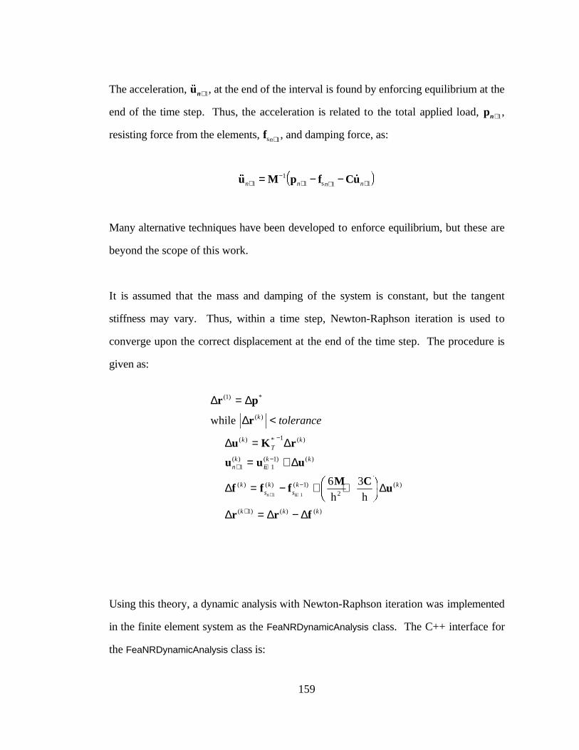
The acceleration, &&un+1, at the end of the interval is found by enforcing equilibrium at the
end of the time step. Thus, the acceleration is related to the total applied load, pn+1,
resisting force from the elements, fsn+1, and damping force, as:
&& &su M p f Cun n n n+−
+ + += − −11
1 1 1c h
Many alternative techniques have been developed to enforce equilibrium, but these are
beyond the scope of this work.
It is assumed that the mass and damping of the system is constant, but the tangent
stiffness may vary. Thus, within a time step, Newton-Raphson iteration is used to
converge upon the correct displacement at the end of the time step. The procedure is
given as:
∆ ∆
∆
∆ ∆
∆
∆ ∆
∆ ∆ ∆
r p
r
u K r
u u u
f f fM C
u
r r f
( ) *
( )
( ) * ( )
( ) ( ) ( )
( ) ( ) ( ) ( )
( ) ( ) ( )
1
1
1 11
12
1
1 1
6 3
=
<
=
= +
= − + +FH
IK
= −
−
+ +−
−
+
+ +
while
h h
k
kT
k
nk
nk k
ks
ks
k k
k k k
tolerance
n n
Using this theory, a dynamic analysis with Newton-Raphson iteration was implemented
in the finite element system as the FeaNRDynamicAnalysis class. The C++ interface for
the FeaNRDynamicAnalysis class is:
159

class FeaNRDynamicAnalysis{// private dataFeaModel* sub; // model to be analyzedchar* lc; // load caseFeaConstraintHandler* conH;// constraint handlerFeaReorderHandler* reoH; // reorder handlerFeaMatrixHandler* matH; // matrix handlerFeaMap* m; // mapdouble lastTime; // previous time valueFeaMatrix* k; // stiffness matrixFeaMatrix* mass; // mass matrixFeaMatrix* mInv; // decomposed mass matrixFeaMatrix* damp; // damping matrixFeaVector* p; // load vectorFeaVector* d; // displacement vectorFeaVector* v; // velocity vectorFeaVector* a; // acceleration vectorFeaVector* rf; // resisting force vectordouble betaK; // stiffness based damping factordouble betaM; // mass based damping factor
// private methodsvoid assembleK(); // assembl. stiffnessvoid assembleMass(); // assembl. massvoid assembleDamp(); // assembl. dampingvoid assembleTotalLoad(); // assembl. total loadvoid assembleTotalLoad(double time);// assembl. total loadvoid assembleResForce(); // assembl. resisting force
public:// constructorFeaNRDynamicAnalysis(FeaModel& model, double bk, double bm);
// initializes the analysisvoid init(char* loadCase);
// performs the analysisvoid analyze(double time);
};
The implementation for the constructor is:
FeaNRDynamicAnalysis(FeaModel& model, double bk, double bm)// constructs an instance of Newton Raphson Dynamic Analysis{
sub = model;betaK = bk;
160

betaM = bm;lastTime = 0.0;
// create the FeaConstraint handlerconH = new FeaTransConHandler(sub);
// create the reordering handlerreoH = new FeaNoOrderHandler(*sub);
// create the mapm = new FeaMap(sub, conH, reoH);
// create the matrix handlermatH = new FeaFullMatrixHandler(m);
// construct the instance variablesk = matH.setupMatrix();mass = matH.setupMatrix();mInv = matH.setupMatrix();damp = matH.setupMatrix();p = matH.setupVector();d = matH.setupVector();v = matH.setupVector();a = matH.setupVector();rf = matH.setupVector();
}
The analysis procedure is broken up into two methods. One to initialize the analysis
(init ), and one to perform the analysis (analyze ). The init method saves the
load case name; assembles the stiffness, mass, and damping matrices; directs the map to
initialize the element states; and creates the inverse of the mass matrix for later use.
The implementation for the init method is:
void init(char* loadCase)// initialize the analysis{
lc = loadCase;
// assemble the stiffness, mass, and dampingassembleK();assembleMass();assembleDamp();
// initialize the element statesm.initializeElSt(lc);
161

// setup and decompose the mInv matrixmInv = mass;mInv.luDecomp();
}
The analyze method advances the state of the analysis, and the Model, to the given
time value. The implementation closely follows the equations given previously.
analyze(double time)// evaluates one time step ending in the given time{
h = time-lastTime // calculate the current time step hpOld = p // save applied loads from last stepassembleLoad(time) // assemble loads into p for this step
// calculate change in rhs of equilibrium equationdeltaR = p - pOld + ( (4.0/h)*v + 2.0*a )*M + 2.0*v*C
// calculate invariant portion of change in velocitydeltaV = - 2.0*v
// calc mc for use inside the loopmc = (4.0/h/h)*M + (2.0/h)*C;
// loop until unbalanced force (deltaR) is smallwhile ( deltaR.norm() < TOLERANCE ){
deltaROld = deltaR // save deltaRassembleK() // assemble stiffnessKstar = K + mc // calculate modified kKstar.luDecomp() // decompose modified kKstar.luForBack(deltaR) // solve for inc in dispd = d + deltaR // update displacementsdeltaV = deltaV + (2.0/h) * deltaR // calc deltaVm.updateDofGroupsByTotal(d) // update nodesm.updateElements() // update elementsrfOld = rf // save old resis. forceassembleResForce() // assem. resis. forcedeltaR = deltaROld - ( rf - rfOld + mc*deltaR)
}v = v + deltaV // calc new velocitiesm.updateDofGroupsDotByTotal(v) // update vel at nodesa = MInv.luForBack(p - rf - C*v) // calc accel from equilm.updateDofGroupsDotDotByTotal(a) // update accel at nodeslastTime = time; // update lastTimem.commit(); // commit state of model
}
162

The total loads are first formed using the assembleLoad method; deltaR is
calculated, and the iteration commences. In each iteration, the stiffness matrix is
formed, the addition displacement is calculated, the state of the Model is updated, the
resisting force, rf , is obtained from the Model, and the remaining unbalanced load is
calculated. When the iteration is complete, the velocities and accelerations at the end
of the time step are calculated, and the Model is updated. Finally, the state of the
Model is committed.
6.2 Substructuring
Substructuring is a process whereby the complete model is broken down into
submodels that are connected at their common nodes. Substructuring is typically
applied when a linear submodel is repeated within an assemblage, such as a multi-span
bridge with identical deck components. The submodels are linear, so it is advantageous
to calculate the properties of the submodel once, and reuse this for all instances of the
submodel.
A submodel is represented to the Model, in which it resides, as a Superelement. The
Superelement provides stiffness, mass, damping, and resisting force to the Nodes in the
Model to which it attaches, in the same way as an Element. In fact, a Superelement is
an Element. This relationship was demonstrated in the entity relationship diagram for
the element object as Figure 4.2.2a. The figure is repeated here for clarity as Figure
6.2a.
163

has a
loaded by
Truss Bar
initiallized by
connects toElement
Initial Element State
...Truss BarState
SuperElementState
...SuperElement
Model
Node
has a
Element Load
...Truss BarLoad
SuperElementLoad
Constitutive Model
Material
calibrated by
Figure 6.2a Entity Relationship Diagram for the Element Object
A Superelement is a type of Element that is contained in a Model. A Superelement also
has a Model. The contained Model object represents a submodel which is hidden from
the Model in which the Superelement resides. This recursive relationship between
Superelements and Models can create any number of levels of substructuring. To
represent the initial state and loads within the submodel, a Superelement may be
associated with SuperElementInitialState and SuperElementLoad objects.
The Superelement is a subclass of the abstract Element class so it must implement all
the methods of the Element class defined in Table 4.2.2. The table is shown again
below as Table 6.2a.
164

Method Arguments Return PurposeConstruction Unique to each element, but
includes instances of
Constitutive Models
Creates an instance of a
specific type of Element
getStiff Stiffness matrix augmented
with transformation into
known Coord Sys
Provides the current linearized
stiffness
getDamp Damping matrix augmented
with transformation into
known Coord Sys
Provides the current linearized
Damping matrix
getMass Mass matrix augmented with
transformation into known
Coord Sys
Provides the current linearized
Mass matrix
getResistingForce Load vector augmented with
Coord Sys
Provides the current resisting
force, including the initial state
and element loads
updateState Causes the Element to update
its state from the Nodes
getEventFactor Event Factor Returns the current event
factor
initialize Unique to each type of
Element
Announces the presence of an
Initial Element State
commitState Commits the current state of
the Element
getConnectingDof list of dof Returns a list of dof to which
the element attaches
Table 6.2a Element Interface Definition
In order to represent the submodel as an Element, the Superelement must be able to
update the state of the submodel according to the state of the model, and communicate
the properties of the submodel to the model. As shown in Figure 6.2b, a submodel
consists of internal degrees of freedom (ui ), which are unique to the submodel, and
external degrees of freedom (ue), which are associated with degrees of freedom in the
model. To update the state of the submodel, the Superelement obtains the response
values of the model degrees of freedom, interprets them in terms of the external
degrees of freedom of the submodel, and calculates the values for the internal degrees
of freedom. To communicate the properties of the submodel to the model, the
165

Superelement transforms the properties of the submodel into external degree of
freedom measures.
ue ue
ui
Figure 6.2b Internal and External Degrees of Freedom for a Submodel
The complete set of degrees of freedom for the submodel can be represented as:
u
ue
i
L
NM
O
QP
Similarly partitioning the equation of equilibrium produces:
K K
K K
u
u
f
fee ei
ie ii
e
i
e
i
L
NM
O
QPL
NM
O
QP = L
NM
O
QP
Through the process of static condensation, the properties of the submodel can be
represented in terms of the external degrees of freedom as:
K T KT
M T MT
C T CT
F T F
T
T
T
T
*
*
*
*
=
=
=
=
166

where:
TI
K Kii eiT=
−L
NM
O
QP−1
The displacements for the complete set of degrees of freedom can be represented by
the external degree of freedom displacements by:
u
uTu
K fe
ie
ii i
L
NM
O
QP = + L
NM
O
QP−
01
Substructuring has been implemented in the finite element program in C++ using three
different objects. The FeaSuperElement object implements the Superelement, the
FeaSuperElementLoad object handles the loads within the submodel, and the
FeaSuperElementInitialState object handles the initial states of the Elements within the
submodel.
6.2.1 FeaSuperElement
The implementation of the FeaSuperElement object deals primarily with the details of
the creation of the previously defined transformation matrix, T, and its application to
the properties of the submodel. The C++ interface for the FeaSuperElement object is
shown below:
class FeaSuperElement : public FeaElement {// private instance variables
// list of nodes in modelList<FeaDofGroup*>* modelNodes;// list of ext nodes in submodel
167

List<FeaDofGroup*>* subModelNodes;FeaModel* subModel; // submodelFeaConstraintHandler* conH;// constraint handlerFeaReorderHandler* reoH; // reorder handlerFeaMatrixHandler* matH; // matrix handlerFeaMap* subMap; // map for the submodelFeaTransformation* trans; // augmented transformation matrixint numExt; // number of external equationint numEq; // total number of equationsint numBlocks; // number of blocks in transFeaMatrix* kiiDecomp; // decomposed kii matrixFeaVector* oldDisp; // old displacements (used by getEF)FeaVector* fi; // internal force vectordouble currentTime; // current time valuechar* loadCase; // current load casechar* initialStateCase; // load case for initial states
// private methodsFeaVector& getdExt();void setUpT();
public:// constructorFeaSuperElement(const char*, FeaModel&, List<FeaDofGroup*>&,
List<FeaDofGroup*>&);
void updateState();void commitState();FeaAugmentedVector& getResistingForce();
FeaAugmentedMatrix& getStiff();FeaAugmentedMatrix& getMass();FeaAugmentedMatrix& getDamp();
void setLoad(char*);void setLoad(char*, double);void setInitialState(char*);
double getEventFactor();
};
A Superelement is constructed by providing the Model object that forms the submodel,
a list of Nodes in the Model to which the Superelement attaches, and the corresponding
list of Nodes in the submodel. The implementation for the constructor is shown below.
The Superelement treats the submodel in a manner similar to the treatment of a Model
168

by an Analysis object. The Superelement creates a Constraint Handler, Reorder
Handler, Matrix Handler, and a Map for the submodel. In this implementation of a
Superelement, the formation of the transformation matrix requires a partitioning of the
submodel's stiffness matrix to isolate the connecting-node degrees of freedom from the
internal-node degrees of freedom. To accomplish this, a FeaDefinedOrderHandler is
chosen. It is given the list of connecting Nodes in the submodel, and will ensure that
these degrees of freedom are numbered before the degrees of freedom in the internal
nodes. Finally, the constructor for the Superelement invokes the setUpT method to
create the transformation matrix.
FeaSuperElement(const char* s, FeaModel& smod, List<FeaDofGroup*>&modNodes, List<FeaDofGroup*>& subModNodes) : FeaElement(s)// constructor for the FeaSuperElement class{
subModel = &smod; // model for the submodelsubModelNodes = &subModNodes; // list of ext nodes in subModelmodelNodes = &modNodes; // corres. list of nodes in model
// construct the constraint handler for the subModelconH = new FeaTransConHandler(*subModel);
// construct the reorder handler for the subModel with the dof// from the external nodes of the subModel numbered in order// firstreoH = new FeaDefinedOrderHandler(*subModel, *subModelNodes);
// construct the map for the subModelsubMap = new FeaMap(*subModel, *conH, *reoH);
// construct the matrix handler for the subModelmatH = new FeaFullMatrixHandler(*subMap);
// set up the dimensions of the problem// (numEq, numExt, numBlocks)numEq = subMap->numEq(); // number of equations for subModelnumExt = 0; // number of eq for ext dofnumBlocks = 0; // number of blocks for transitr(*subModelNodes); // create iter for subModel nodes// iterate through the subModel nodes to create numExt and// numBlocksiterateThrough ( itr ) // itr() is FeaDofGroup object{
169

// get the list of FeaDof descriptions from the node// and iterate thru ititr1 = itr().getDescItr(); // create iter for dof desc// iterate through the dof desc at the nodeiterateThrough ( itr1 ) // itr1() is a FeaDofDesc object{
numExt += itr1().nDof(); // add # of componentsnumBlocks++; // add a block for desc
}}
oldDisp = new FeaFullVector(numEq); // set up oldDisp vector
setUpT(); // set up the trans instance variable}
The setUpT method constructs the FeaTransformation object trans , which is used to
transform the properties of the submodel from a submodel basis to a model basis. The
implementation for the setUpT method is shown below. A FeaTransformation object
must be used by all Elements to convey property matrices and vectors to the Map. A
FeaTransformation object contains the transformation matrix, in the form of a block
matrix, and a list of Degree of Freedom Descriptions, which label the column blocks.
To form the transformation matrix, the stiffness matrix for the submodel is formed into
a 2 by 2 block matrix, partitioned according to the division of internal and external
degrees of freedom. The columns of the transformation matrix are then built along
with the degree of freedom descriptions. With trans defined in this manner, it can be
used directly by the getStiff , getMass , getDamp , and
getResisitingForce methods.
void setUpT()// sets up the trans instance variable{
k(numExt-1, numExt-1) = 0.0; // set up K as 2x2 block matrixk(numEq-1, numEq-1) = 0.0;
//assemble the complete stiffness matrixitre = subMap.elementItr(); // itre() is an FeaElementiterateThrough (itre)
170

{kel = subMap.getElStiff( itre() );k.assemble( kel.getTransformedK(), kel.getId() );
}
kei = k.getBlock(0,1); //separate components of Kkii = k.getBlock(1,1);kii.luDecomp(); // Decompose Kii
// set up the transformation matrix block by block// numBlocks along the columns and 1 block down the rowscurColOfT = 0;trans = new FeaTransformation(1,numBlocks);// iterate thru the list of nodes in the subModel and Model// simultaneouslyitrSub(subModelNodes); // create iterator for subModel NodesitrMod(modelNodes); // create iterator of Model NodesitrMod.init(); // initiate the model node iterator
// iterate through the sub model nodesiterateThrough (itrSub){
// get the list of Dof descriptions from the node// and iterate thru ititr1 = itrSub().getDescItr(); // iter for submodel desc.itr1Mod = itrMod().getDescItr(); // iter for model desc.itr1Mod.init(); // initiate the model desc.
// iterate through sub modeliterateThrough ( itr1 ){
// block is numEq by number of dof to represent//the vector in the coord syst = new FeaFullMatrix(numEq,itr1().nDof());for ( int i = 0; i < itr1()->nDof(); i++ ){
tmp = new FeaFullVector(numEq-numExt);// place portion of kei in tmpint j;for ( j = 0; j < numEq - numExt; j++){
tmp(j) = -kei(curColOfT,j);}// solve to get -kii^-1 * kei^tkii.luForBack(*tmp);// place a one for the external dof to be retainedt(curColOfT,i) = 1.0;// place -kii^-1 * kei^t in tfor ( j = 0; j < numEq - numExt; j++){
t(numExt+j,i) = tmp(j);}
171

curColOfT++;}// create description for the blockdI = FeaTransDesc(itr1().getType(), itrMod(),
itr1().getCoOrdSys());// add description and transformation block to transtrans.addDesc(*dI, *t);++itr1Mod; // increment the iterator for the model desc.
}++itrMod; // increment the iterator for the model nodes
}}
With the trans object defined, the work of the Superelement is straight forward.
When a given property is requested, the Superelement forms the property of the
submodel using the submodel's Map object, attaches a copy of the trans object to it,
and passes back the result. For example, the implementation for the
getResistingForce method is:
FeaAugmentedVector& getResistingForce(){ //assemble the complete resisting force vector p p = new FeaFullVector(numEq);
// add in the nodal forces for the subModel itr1 = subMap.loadItr(loadCase); // get iter for loads iterateThrough ( itr1 ) // itr1() is a FeaLoad object { ldv = subMap.getLoad( itr1(), currentTime ); p.assemble( ldv.getTransformedLoad(), ldv.getId() ); }
// assemble the element resisting forces for the subModel itr = subMap.elementItr(); // get iter for the elements iterateThrough ( itr ) // itr() is a FeaElement { ldv = subMap.getResistingForce( itr() ); p.assemble( ldv.getTransformedLoad(), ldv.getId() ); }
// save force vector for getdExt() method fi = p;
172

// create and return the augmented Vector return (new FeaAugmentedVector(p, trans));}
First, a vector p is created. An iterator for the Elements in the submodel is obtained
from the submodel's Map. One by one, the resisting force vectors from the Elements of
the submodel are obtained and assembled into p. The nodal forces applied to the
submodel for the active Load Case are then added to p. The resisting force vector is
saved as fi for later processing by the getdExt method. The FeaAugmentedVector
object is formed by using p and a copy of trans . This is returned to the caller of the
method. The methods for mass, damping, stiffness, and load follow in a similar
manner.
FeaAugmentedMatrix& getStiff(){
k = new FeaFullMatrix(numEq, numEq); // stiffness matrix
// iterate thru the Elements and assemble stiffnessitr = subMap.elementItr(); // get iter for elementsiterateThrough ( itr ) // itr() is a FeaElement{
kel = subMap.getElStiff( itr() );k.assemble( kel.getTransformedK(), kel.getId() );
}
// create and return augmented stiffness matrixreturn (new FeaAugmentedMatrix(k, trans));
}
FeaAugmentedMatrix& getMass(){
mass = new FeaFullMatrix(numEq, numEq); // mass matrix
// iterate thru the Elements and assemble massitr = subMap.elementItr(); // get iter for elementsiterateThrough ( itr ) // itr() is a FeaElement{
kel = subMap.getMass( itr() );mass.assemble( kel.getTransformedK(), kel.getId() );
}
// create and return augmented mass matrix
173

return (new FeaAugmentedMatrix(mass, trans));}
FeaAugmentedMatrix& FeaSuperElement::getDamp(){
damp = new FeaFullMatrix(numEq, numEq); // damp matrix
// iterate thru the Elements and assemble dampingitr = subMap.elementItr(); // get iter for elementsiterateThrough ( itr ) // itr() is a FeaElement{
kel = subMap.getDamp( itr() );damp.assemble( kel.getTransformedK(), kel.getId() );
}
// create and return augmented damping matrixreturn (new FeaAugmentedMatrix(damp, trans));
}
The updateState , commitState and getEventFactor methods in the
Superelement require that the Nodes of the submodel be updated with the response
values of the Nodes in the Model. To perform this function, the getdExt method is
provided. The getdExt method queries the Nodes in the Model to which the
Superelement attaches; assembles a vector of displacements of these Nodes in terms of
the unknowns in the Superelement. The method simultaneously loops through the list
of corresponding Nodes in the model and submodel, queries the model Nodes as to
their current total displacement vectors, interprets the vectors in terms of the
coordinate systems at the corresponding submodel Node, and places the components in
the appropriate location of the displacement vector. The displacements for the internal
degrees of freedom in the submodel are determined from:
u
uTu
K fe
ie
ii i
L
NM
O
QP = + L
NM
O
QP−
01
Both T and Kii−1 are generated and stored in the Superelement by the setupT method.
fi is stored in the Superelement by the getResistingForce method. The
174

complete displacement vector for the submodel is returned. The implementation for
the getdExt method is shown below:
FeaVector& getdExt()// returns a vector representing the current external// displacements. The ordering of dExt is defined by the// reorder handler chosen (FeaDefinedOrder){
dExt = new FeaFullVector(numExt); // set up the return valuecount = 0; // counter for the placement of dof values in dExt
// iterate over the model nodes and external submodel nodes// simultaneouslyitr(modelNodes); // create iterator for model NodesitrSub(subModelNodes); // create iterator of submodel NodesitrSub.init(); // initiate submodel node iterator
// iterate through the submodel nodesiterateThrough ( itr ){
// get the list of Dof descriptions from the node// and iterate thru ititr1 = itr().getDescItr(); // iter for model descitr1Sub = itrSub().getDescItr(); // iter for submodel descitr1Sub.init(); // initiate submodel desciterateThrough ( itr1 ){
// get the current total disp vector from the model and// interpret it in terms of the coordinate system at the// associated subModel noded1 = ( itr().getTotalV(itr1().getType()) )
.get_rep_in(itr1Sub().getCoOrdSys());// loop through d1 and place the results in dExtfor ( int i = 0; i < d1.getSize(); i++ ){
dExt(count) = d1(i);count++; // increment placement counter
}++itr1Sub; // increment the submodel node desc iter
}++itrSub; // increment the submodel node iter
}return dExt; // return the displacement vector
}
175

The updateState method calls the submodel Map's
updateDofGroupsByTotal method with the complete displacement vector of the
submodel as an argument. The Elements of the submodel are then updated by the
submodel Map. The implementation for the updateState method is shown below:
void updateState(){
//get model dof statedExt = getdExt();
//transform to complete total displacementDisp = trans.getTrans() * dExt;
//update submodelsubMap.updateDofGroupsByTotal(Disp);
// save displacements for event factor calcoldDisp = Disp;
//update element statesubMap.updateElements();
}
The commitState method is similar except that the Nodes and Elements of the
submodel are committed by the submodel Map object. The implementation for the
commitState method is shown below:
void FeaSuperElement::commitState(){
//get model dof statedExt = getdExt();
//transform to complete total displacementDisp = trans.getTrans() * dExt;
//update submodelsubMap.updateDofGroupsByTotal(Disp);
// save displacements for event factor calcoldDisp = Disp;
// commit the nodes and elements
176

subMap.commit();
}
The getEventFactor updates the nodal displacements using the
updateDofGroupsByTotal method of the submodel Map with the total
displacements obtained from the getdExt method as an argument. It then instructs
the submodel Map to query the Elements and obtain the smallest event factor. Upon
completion of the method, the submodel Nodes are returned to their previous state
using the oldDisp instance variable (which is kept up by the update and commit state
methods). The implementation for the getEventFactor method is shown below:
double FeaSuperElement::getEventFactor(){
//get model dof statedExt = getdExt();
//transform to complete total displacementDisp = trans.getTrans() * dExt;
//update submodelsubMap.updateDofGroupsByTotal(Disp);
// calc event factor for elementsfactor = subMap.getMinEventFactor();
// return the nodes to their previous statesubMap.updateDofGroupsByTotal(oldDisp);
return factor;}
The setInitialLoad method is called by the FeaSuperElementInitialState object. It
is passed the name of the Load Case in the submodel that contains the initial element
state information. The setInitialState method obtains the initial element state
iterator from the submodel's Map. It then iterates through the list of Initial Element
State objects and calls the initialize method; thereby initializing the state of the
177

Elements of the submodel. The implementation for the setInitialLoad method is
shown below:
void setInitialLoad(char* loadCase){
// iterate through the initial element states in the load caseitr = subMap.initElStItr(loadCase); // iter for init El StateiterateThrough ( itr ) // itr() is a FeaInitElState object{
itr().initialize();}
}
The setLoad method is called by the FeaSuperElementLoad object. It is passed the
name of the Load Case in the submodel that is to be applied to the submodel. The
setLoad method then obtains the load iterator from the submodel's Map and iterates
through the list of Loads, invoking their getLoad method. This sets up both the
Element and Nodal Loads with the correct values of time for later processing by the
getResisitingForce method.
void setLoad(char* loadCase, double time = 0.0){
currentTime = time; // save time for use by resisting force
// iterate through the loadsitr = subMap.loadItr(loadCase); // iter for the loadsiterateThrough ( itr ){
itr().getLoad(time); // element, thus no load is returned}
}
178

6.2.2 FeaSuperElementLoad
The purpose of the FeaSuperElementLoad object is to maintain the name of the
submodel Load Case that describes the Loads on the Elements and Nodes of the
submodel. The FeaSuperElementLoad object will itself be held in a Load Case for the
complete model. Upon initialization, the FeaSuperElementLoad object registers its
presence with the Superelement to which it applies, and gives the Superelement the
name of the submodel Load Case. The Superelement will use this information to
include the loads in the resisting force computation. The FeaSuperElementLoad class is
slightly different from other Element Load classes in that there is only one type of
loading for a Superelement. Other Element types can have any number of different
types of element loads. For example, a Truss Bar could have both uniform load or
point load types of element loading.
The C++ interface for the FeaSuperElementLoad object and the implementation for its
methods are shown below:
class FeaSuperElementLoad : public FeaElementLoad {FeaSuperElement* el; // element to which the load applieschar* subModelLoadCase; // name of the load case in the subModeldouble time; // current value of timepublic:
// constructorFeaSuperElementLoad(FeaSuperElement&, char*);
// methods to return the current loadsFeaAugmentedVector& getLoad();FeaAugmentedVector& getLoad(double);
};
FeaSuperElementLoad(FeaSuperElement& ne, char* s)// constructor for FeaSuperElementLoad{
el = ne; // superElement to be loadedsubModelLoadCase = s;// load case name
}
179

FeaAugmentedVector& getLoad()// sets up the superelement for the load and returns zero{
el.setLoad(subModelLoadCase);return NULL;
}
FeaAugmentedVector& getLoad(double time)// sets up the superelement for the load and returns zero{
el.setLoad(subModelLoadCase, time);return NULL;
}
6.2.3 FeaSuperElementInitialState
The purpose of the FeaSuperElementInitialState object is to maintain the name of the
submodel Load Case that describes the initial states of the Elements of the submodel.
The FeaSuperElementInitialState object will itself be held in a Load Case for the
complete model. Upon initialization, the FeaSuperElementInitialState object registers its
presence with the Superelement to which it applies, and gives the Superelement the
name of the submodel Load Case that holds the Initial Element State objects. The
Superelement will use this information to include the initial element states in the
resisting force computation. The FeaSuperElementInitialState class is slightly different
from other Initial Element State classes in that there is only one type of Initial Element
State for a Superelement. Other Element types can have any number of different types
of Initial Element State.
The C++ interface for the FeaSuperElementInitialState object and the implementation for
its methods are shown below:
180

class FeaSuperElementInitialState : public FeaInitialElementState{FeaSuperElement* el; // element that has the initial statechar* subModelLoadCase; // load case that contains the init statepublic:
// constructorFeaSuperElementInitialState(FeaSuperElement&, char*);
// applies the initial stateFeaAugmentedVector& initialize();
};
FeaSuperElementInitialState(FeaSuperElement& ne, char* s)// constructor{
el = ≠ // element with initial statesubModelLoadCase = s;// name of load case
}
void initialize()// initializes the state of the superElement{
el.setInitialLoad(subModelLoadCase);}
6.3 2D Beam Element With End Hinges
One of the more useful elements in the analysis of steel and reinforced concrete frames
is the two-dimensional beam element with hinges at the ends. For steel beams, the
moment rotation constitutive model for the hinges is often assumed as rigid perfectly
plastic. For reinforced concrete, a more complex behavior is often assumed. In either
case, the basic element is identical. The difference lies in the assumptions for the hinge
constitutive model. Thus, it is desirable to produce an Element object that can accept
any moment rotation Constitutive Model.
For this element implementation, an elastic perfectly plastic moment rotation
Constitutive Model was developed. Although it was developed for this element, it
181
conforms to the requirements for moment-rotation Constitutive Models. It can be used
wherever a moment-rotation Constitutive Model is required. Conversely, the Element
can also use any moment-rotation Constitutive Model that is developed in the future.
The 2D Hinged Beam Element has been developed as a planar element, which required
a new 2D rectangular coordinate system. The new coordinate system is a subclass of
the abstract class FeaCoOrdSys. The 2D Hinged Beam Element interfaces with the rest
of the model as if it were in a two-dimensional world. But since the 2D Hinged Beam
Element may be used in a three-dimensional context, the orientation of the strong
bending axis of the beam in 3D must be known. The 2D Hinged Beam Element must
be given a Geometric Point in addition to the Nodes to which it attaches. If the
translational degrees of freedom at the two Nodes lie in the same plane, the additional
Geometric Point is not required. The strong bending axis is assumed to be
perpendicular to the plane of the problem.
6.3.1 Moment-Rotation Elastic-Perfectly Plastic Constitutive Model
A moment-rotation relationship must be described for the hinges at the ends of the
beam. An elastic perfectly plastic relationship will be used to demonstrate the element.
The moment-rotation Constitutive Model is a subclass of the 1D Constitutive Model.
The moment rotation class is further subclassed into the concrete classes
1DMRLinearElastic and 1DMRElasticPerfectlyPlastic, etc.
The methods that a Constitutive Model object must provide to the system are defined
in Table 4.2.3a, and are shown again below as Table 6.3.1a.
182

Method Arguments Return PurposeConstruction Parameters necessary to define
the model, including the
Material
Creates an instance of a
Constitutive Model
setIncV Action/Deformation object
with an array of deformations
Sets the increment of the
current strain state
setTotalV Action/Deformation object
with an array of deformations
Sets the total current strain
state
setInitialV Action/Deformation object
with an array of initial
deformations
Sets the initial state
commit Commits the state
getCurrentPlusDeltaS Action/Deformation
object with an array of
total actions
Returns the total stress state
getCurrentCommittedS Action/Deformation
object with an array of
incremental actions
Returns the last increment in
stress state
getK Constitutive matrix Returns the current
linearization
getEventFactorIncV Action/Deformation object
with an array of deformations
Event Factor Returns the current event
factor
getEventFactorTotalV Action/Deformation object
with an array of deformations
Event Factor Returns the current event
factor
Table 6.3.1a Constitutive Model Interface Definition
A moment-rotation Constitutive Model is responsible for maintaining and reporting on
the state of the moment-rotation relationship. The elastic-perfectly-plastic response for
the model is show below in Figure 6.3.1b. The model can be in one of three states at
any instance: it can be yielding with a negative moment (zone 1); it can be in the elastic
region (zone 2); or it can be yielding with a positive moment (zone 3).
183

M
θ
k1
vSpread
M p
M p
Figure 6.3.1b Elastic-Perfectly-Plastic Moment-Rotation Relationship
A Constitutive Model can initialize, update, commit, and report on its state at the
request of an Element. In accordance with the object design, the Constitutive Model
must remain elastic during an update of its state, but may be inelastic immediately after
its state is committed. The Constitutive Model tracks its last committed state (which
defines the action/deformation curve) and its total state (which defines its position on
the curve). In this case, the last committed state defines the limits of the three zones.
The current state is on the moment-rotation curve defined by the last committed state.
When the model is instructed to commit its state, it must save the current state as the
committed state, and adjust the limits of the three zones. If it is in a plastic zone (1 or
3), the limits of the zones are adjusted such that a reversal in rotation will cause the
model to enter the elastic zone (zone 2).
The state of the model is updated by adding to the current rotation by either specifying
a new increment in rotation from the last committed state or a new total rotation. For
either case, the model must track the new current state and the zone in which it resides.
The model calculates the resisting moment based on the zone for either the current
184

state or the last committed state as requested. The stiffness of the model is reported
based on the current state.
The event factor is defined as the proportion of the difference between the current state
and the last committed state that can be accommodated without crossing the
boundaries of a zone. The event factor can be obtained by specifying either a new
increment in rotation from the last committed state or a new total rotation. This new
rotation is used only for the event factor calculation, and does not affect the state of the
model.
The elastic perfectly plastic moment rotation Constitutive Model is implemented as the
Fea1DMRotElasticPlastic class. The C++ interface for the class is:
class Fea1DMRotElasticPlastic : public Fea1DConstitutiveModel{double currentV; // current committed value of rotationdouble deltaV; // current change in rotation from the
// committed to the totaldouble initialV; // initial value of rotationdouble k1; // elastic stiffnessdouble vChangePos;// current upper elastic rotation limitdouble vChangeNeg;// current lower elastic rotation limitdouble vSpread; // elastic rotation range (does not vary)int curZone; // current committed zone:
// 1 - -ve , 2- elastic, 3- +veint totalZone; // total zone: 1 - -ve , 2- elastic, 3- +ve
public:// constructorFea1DMRotElasticPlastic(double stiffness1,
double Myield);// copies the instanceFea1DConstitutiveModel& copy();
// update and commit statevoid setIncV(double);void setTotalV(double);void setInitialV(double);void commit();
// returns the required moment
185

double getCurrentCommittedS();double getCurrentPlusDeltaS();
// return the current stiffnessdouble getK();
// return the event factor given a new increment or total rot.double getEventFactorIncV(double);double getEventFactorTotalV(double);
};
The implementation of the class is fairly straightforward. The limits of the zones are
defined by the instance variables vChangePos , vChangeNeg , and vSpread . The
last committed state is defined by currentV . The current state is not stored directly,
rather the difference between the current state and the last committed state is stored as
deltaV . The implementation for the methods is shown below:
Fea1DMRotElasticPlastic(double stiffness1, double Myield)// creates an instance of the class{
k1 = stiffness1;vChangePos = Myield/k1;vChangeNeg = -Myield/k1;vSpread = 2.0 * Myield/k1;previousV = 0.0;currentV = 0.0;deltaV = 0.0;initialV = 0.0;curZone = 2;totalZone = 2;
}
Fea1DConstitutiveModel& copy()// creates a copy (useful when the client is not aware of the// actual subclass of constitutive model being held{
return *(new Fea1DMRotElasticPlastic(*this));}
void setIncV(double nv)// update state by specifying a new increment in rotation{
deltaV = nv;// set totalZone
186

double totalV = initialV + currentV + deltaV;if ( totalV >= vChangePos ) totalZone = 3;else if ( totalV <= vChangeNeg ) totalZone = 1;else totalZone = 2;
}
void setTotalV(double nv)// update state by specifying a new total rotation{
deltaV = nv - currentV;// set totalZonedouble totalV = initialV + currentV + deltaV;if ( totalV >= vChangePos ) totalZone = 3;else if ( totalV <= vChangeNeg ) totalZone = 1;else totalZone = 2;
}
void setInitialV(double nv)// sets the initial rotation{
initialV = nv;}
void commit()// commits the current state{
double v = initialV + currentV;switch (curZone) {case 1:
switch (totalZone) {case 1:
vChangeNeg = v+deltaV;vChangePos = vChangeNeg + vSpread;break;
case 2:curZone = 2;break;
case 3:vChangePos = v + deltaV;vChangeNeg = vChangePos - vSpread;curZone = 3;break;
}break;
case 2:switch (totalZone) {case 1:
vChangeNeg = v+deltaV;vChangePos = vChangeNeg + vSpread;curZone = 1;break;
case 2:
187

break;case 3:
vChangePos = v + deltaV;vChangeNeg = vChangePos - vSpread;curZone = 3;break;
}break;
case 3:switch (totalZone) {case 1:
vChangeNeg = v+deltaV;vChangePos = vChangeNeg + vSpread;curZone = 1;break;
case 2:curZone = 2;break;
case 3:vChangePos = v + deltaV;vChangeNeg = vChangePos - vSpread;break;
}break;
}
previousV = currentV;currentV += deltaV;deltaV = 0.0;
}
double getCurrentCommittedS()// returns the current committed moment value{
double v = initialV + currentV;double ans;if ( v <= vChangePos && v >= vChangeNeg )
ans = k1*(v - (vChangePos+vChangeNeg)/2.0);else{
if ( (v) > vChangePos )ans = k1*(vChangePos-vChangeNeg)/2.0;
elseans = -k1*(vChangePos-vChangeNeg)/2.0;
}return ans;
}
double getCurrentPlusDeltaS()// returns the total moment value (committed + delta){
double v = initialV + currentV + deltaV;
188

double ans;switch (totalZone) {case 1:
ans = -k1*vSpread/2.0;break;
case 2:ans = k1*(v - (vChangePos-vSpread/2.0));break;
case 3:ans = k1*vSpread/2.0;break;
}return ans;
}
double getK(){
double ans;if ( totalZone == 2 ) ans = k1;else ans = 0.0;return ans;
}
double getEventFactorIncV(double nv)// returns the event factor for a new specified increment rot.{
double ans;double lastIncV = nv;double totalV = initialV+currentV + nv;
if (lastIncV == 0.0) ans = 1.0;else{
switch (curZone) {case 1:
if ( totalV <= vChangeNeg )ans = 1.0; // does not hit vChangeNeg, no event
elseans = 0.0;
break;case 2:
if ( (totalV > vChangeNeg) && (totalV < vChangePos) )ans = 1.0; // stays within curZone 2, no event
else{
if ( totalV >= vChangePos )// goes over vChangePosans = (vChangePos - (initialV+currentV)) /
lastIncV;else // goes under vChangeNeg
ans = ((initialV+currentV) - vChangeNeg) /(-lastIncV);
}
189

break;case 3:
if ( totalV >= vChangePos )ans = 1.0; // does not hit vChangePos, no event
elseans = 0.0;
break;}
}
return fabs(ans);}
double getEventFactorTotalV(double nv)// returns the event factor for a specified total rotation{
double ans;double lastIncV = nv - currentV;double totalV = initialV+nv;
if (lastIncV == 0.0) ans = 1.0;else{
switch (curZone) {case 1:
if ( totalV <= vChangeNeg )ans = 1.0; // does not hit vChangeNeg, no event
elseans = 0.0;
break;case 2:
if ( (totalV > vChangeNeg) && (totalV < vChangePos) )ans = 1.0; // stays within curZone 2, no event
else{
if ( totalV >= vChangePos ) // goes over vChangePosans = (vChangePos - (initialV+currentV)) /
lastIncV;else // goes under vChangeNeg
ans = ((initialV+currentV) - vChangeNeg) /(-lastIncV);
}break;
case 3:if ( totalV >= vChangePos )
ans = 1.0; // does not hit vChangePos, no eventelse
ans = 0.0;break;
}}
190

return fabs(ans);}
6.3.2 2D Rectangular Coordinate System
The geometry of the 2D Hinged Beam Element is defined by two Nodes, which
describe the axis of the beam, and an additional Geometric Point that lies in the plane
that is perpendicular to the strong bending axis of the beam. The deformation of the
beam is obtained from the finite element system by means of Geometric Vectors
formulated within Coordinate Systems. The rotational component of deformation is
one-dimensional. The previously defined 1D rectangular Coordinate System class may
be used for this purpose. The translational component of deformation is two-
dimensional. A new 2D rectangular Coordinate System class in needed.
The methods that a Coordinate System object must provide are defined in Table 4.4.1a,
and are shown again below as Table 6.3.2a.
Method Arguments Return PurposeConstruction parameters unique to the
specific System that relate it to
the global system
Creates an instance of a
specific type of Coordinate
System
num_of_axis number of axis Returns the number of axis in
the Coordinate System
trans_to_global transformation matrix Returns the transformation
matrix to convert ordinates in
this system to the Global
trans_from_global transformation matrix Returns the transformation
matrix to convert ordinates in
Global system to this system
Table 6.3.2a Coordinate System Interface Definition
191

A Coordinate System object is responsible for storing and reporting on its rotational
positioning relative to a 3D rectangular global Coordinate System. This is
accomplished by maintaining a rotation matrix of direction cosines that can transform
the ordinates of a point in the system to that in the global system. The format of the
rotation matrix is:
rotation =
C C
C C
C C
where C is the cosine of the angle
the i -axis of the global system and
the j- axis of the local system
11 12
21 22
31 32
ij
L
N
MMM
O
Q
PPP
The calculation of the direction cosines is given in literature Beaufait et al [5]. The
rotation matrix itself provides the transformation matrix to global coordinates, while its
transpose provides the transformation matrix from global coordinates.
The two-dimensional rectangular Coordinate System was implemented as the
Fea2DRect class. The C++ interface for the class is:
class Fea2DRect : public FeaCoOrdSys {FeaFullMatrix* rot; // matrix of direction cosines
public:// constructorsFea2DRect();Fea2DRect(FeaFullVector&);Fea2DRect(FeaGeoPoint&, FeaGeoPoint&, FeaGeoPoint&);
// transformationsFeaFullMatrix& get_trans_to(Fea2DRect&);FeaFullMatrix& trans_to_global();FeaFullMatrix& trans_from_global();int num_of_axis();
192

// copies the instanceFeaCoOrdSys& copy();
};
The implementation of the Fea2DRect class is fairly straightforward. Two constructors
are provided. The first takes a vector of length 3, which defines the three sequential
rotation angles, in radians, about the 3, 1, and 2 axis necessary to align the global
system with the defined system. These angles directly define the rotation matrix. The
second constructor takes three Geometric Points as its arguments. The Points
represent the origin of the Coordinate System, a Point along the positive 1-axis, and a
Point along the positive 2-axis, respectively. The implementation for the methods is
shown below:
Fea2DRect()// gives global coord system{
rot = new FeaFullMatrix(2,3);rot(0,0) = 1.0;rot(1,1) = 1.0;
}
Fea2DRect(FeaFullVector& rv)// sets up rot which is the trans to this system from global// Taken from "Computer Methods of Structural Analysis",// Beaufait et al pg. 240{
rot = new FeaFullMatrix(2,3);
cx = cos(rv(1)) * cos(rv(0));cy = sin(rv(1));cz = cos(rv(1)) * sin(rv(0));
lxz = sqrt( cx*cx + cz*cz );
cp = cos(rv(2));sp = sin(rv(2));
if ( lxz > YAXISTOL ) // Y-Z-X transformation{
rot(0,0) = cx;rot(0,1) = cy;rot(0,2) = cz;
193

rot(1,0) = ( -cx*cy*cp - cz*sp ) / lxz;rot(1,1) = lxz * cp;rot(1,2) = ( -cy*cz*cp + cx*sp ) / lxz;
}else // Z-Y-X transformation{
lxy = sqrt( cx*cx + cy*cy );rot(0,0) = cx;rot(0,1) = cy;rot(0,2) = cz;rot(1,0) = ( -cx*cz*sp - cy*cp ) / lxy;rot(1,1) = ( -cy*cz*sp + cx*cp ) / lxy;rot(1,2) = lxy * sp;
}}
Fea2DRect(FeaGeoPoint& n1, FeaGeoPoint& n2, FeaGeoPoint& n3)// 1-axis from n1 to n2, n3 defines the plane formed// by the 1-2 axis// Taken from "Computer Methods of Structural Analysis",// Beaufait et al pg. 243{
rot = new FeaFullMatrix(2,3);
double l = n1.lengthTo( n2 );xyz1 = n1.get_rep_in();xyz2 = n2.get_rep_in();xyz3 = n3.get_rep_in();
cx = ( xyz2(0) - xyz1(0) ) / l;cy = ( xyz2(1) - xyz1(1) ) / l;cz = ( xyz2(2) - xyz1(2) ) / l;
lxz = sqrt( cx*cx + cz*cz );
if ( lxz > YAXISTOL ) // Y-Z-X transformation{
double yp = -cx*cy*xyz3(0)/lxz + lxz*xyz3(1) -cy*cz*xyz3(2)/lxz;
double zp = -cz*xyz3(0)/lxz + cx*xyz3(2)/lxz;
double lyz = sqrt( yp*yp + zp*zp );
double cp = yp/lyz;double sp = zp/lyz;
rot(0,0) = cx;rot(0,1) = cy;rot(0,2) = cz;rot(1,0) = ( -cx*cy*cp - cz*sp ) / lxz;rot(1,1) = lxz * cp;rot(1,2) = ( -cy*cz*cp + cx*sp ) / lxz;
194

}else // Z-Y-X transformation{
yp = xyz3(1) - xyz1(1);zp = xyz3(2) - xyz3(2);
lyz = sqrt( yp*yp + zp*zp );
cp = yp/lyz;sp = zp/lyz;
lxy = sqrt( cx*cx + cy*cy );
rot(0,0) = cx;rot(0,1) = cy;rot(0,2) = cz;rot(1,0) = ( -cx*cz*sp - cy*cp ) / lxy;rot(1,1) = ( -cy*cz*sp + cx*cp ) / lxy;rot(1,2) = lxy * sp;
}}
FeaCoOrdSys& copy(){
return (new Fea2DRect(this));}
FeaFullMatrix& get_trans_to(Fea2DRect& dest){
return (dest.trans_from_global() * rot);}
FeaFullMatrix& trans_to_global(){
return (rot.transpose());}
FeaFullMatrix& trans_from_global(){
return (rot);}
int num_of_axis(){
return(2);}
195

6.3.3 2D Beam Element With End Hinges
Once the Constitutive Model for the hinges and the 2D Rectangular Coordinate System
are defined, the actual 2D Hinged Beam Element can be constructed. Any moment-
rotation Constitutive Model may be assigned to the hinges. The beam segment
between the hinges is assumed to be linear elastic.
The entity relationship diagram for the 2D Hinged Beam Element is shown in Figure
6.3.3a. The 2D Hinged Beam Element is a subclass of the abstract Element class. For
the current implementation, the Initial Element State and Element Load objects are not
defined.
initiallized by
connects toElement
Initial Element State
...2D BeamState
Truss BarState
...2D HingedBeamTruss Bar
Model
Node
loaded by
Element Load
...2D BeamLoad
Truss BarLoad
Constitutive Model
Material
calibrated by
Figure 6.3.3a Entity Relationship Diagram for the 2D Beam Element with End
Hinges
196

Since the 2D Hinged Beam Element is a subclass of the Element class, it must
implement all the methods of the Element class defined in Table 4.2.2. The table is
shown again below as Table 6.3.3a.
Method Arguments Return PurposeConstruction Unique to each Element, but
includes instances of
Constitutive Models
Creates an instance of a
specific type of Element
getStiff Stiffness matrix augmented
with transformation into
known Coord Sys
Provides the current linearized
stiffness
getDamp Damping matrix augmented
with transformation into
known Coord Sys
Provides the current linearized
Damping matrix
getMass Mass matrix augmented with
transformation into known
Coord Sys
Provides the current linearized
Mass matrix
getResistingForce Load vector augmented with
Coord Sys
Provides the current resisting
force, including the initial state
and element loads
updateState Causes the Element to update
its state from the Nodes
getEventFactor Event Factor Returns the current event
factor
initialize Unique to each type of
Element
Announces the presence of an
Initial Element State
commitState Commits the current state of
the Element
getConnectingDof list of dof Returns a list of dof to which
the element attaches
Table 6.3.3a Element Interface Definition
To provide these methods, the 2D Hinged Beam Element must be able to interpret its
state from the connecting Nodes, communicate this state to its Constitutive Model
objects, and be able to report on its state.
The translational and rotational deformations of the Nodes are transmitted via
Geometric Vectors. The Geometric Vectors can be interpreted in any Coordinate
197

System. For a given Coordinate System defined at the Nodes, shown in Figure 6.3.3b,
the deformation Vectors may have three components.
Node i
Node j
Figure 6.3.3b Nodal Coordinate Systems
The 2D Hinged Beam Element will interpret the same deformation Vectors in its own
set of external element Coordinate Systems shown in Figure 6.3.3c. The translational
Coordinate Systems are separate from the rotational ones. Thus, the translational
deformation vector is interpreted in a 2D Coordinate System, while the rotational
deformation vector is interpreted in 1D Coordinate System. The deformations with
respect to the external element Coordinate Systems are placed in the array r .
node i
node j
r2
r1r3
r5 r4r6
Figure 6.3.3c External Element Coordinate Systems
The internal representation of the deformations is more complex due to the possible
nonlinear rotations of the hinges. The internal measures of deformation q are shown in
Figure 6.3.3d.
198

Node i Node j
q1 q4 q5 q2q3
Figure 6.3.3d Internal Measures of Deformation
Using an incremental formulation, the element must transform displacements from ∆r
to ∆q. Due to the nonlinearity in the hinges, this transform may vary during the
analysis. The first three measures of ∆q can be obtained directly from:
∆q1 = ∆r3 - ( ∆r5 - ∆r2 ) / l
∆q2 = ∆r6 + ( ∆r5 - ∆r2 ) / l
∆q3 = ∆r4 - ∆r1
The fourth and fifth measures of ∆q are recovered from:
∆q4
∆q5
= k-1
ki ∆q1
kj ∆q2
Where ki and kj are the current hinge stiffnesses and k is the 2 by 2 elastic beam
stiffness matrix. The change in rotation of the hinges is then defined as:
∆rotationi = ∆q4 - ∆q1
∆rotationj = ∆q2 - ∆q5
The current linearized stiffness of the 2D Hinged Beam Element is obtained through
static condensation as:
199

ki -(k-1)11ki2 -(k-1)12kikj 0 kj -(k-1)11kj
2 0 AE/l
The change in resisting force is obtained as:
∆Mi = ki ∆rotationi
∆Mj = kj ∆rotationj
The interface for the 2D Hinged Beam Element is shown below.
class FeaHingedBeamColumn : public FeaElement {FeaNode* nodeI; // connecting node IFeaNode* nodeJ; // connecting node JFea1DConstitutiveModel* hingeI; // materialFea1DConstitutiveModel* hingeJ; // materialFea1DConstitutiveModel* axialMat; // materialFea3DRect* mtcs; // 3D translational coord sys for massFea2DRect* tcs; // translational coordinate systemFea1DRect* rcs; // rotational coordinate systemFeaFullMatrix* t;
double area; // Xsect areadouble EA; // Xsect areadouble EI; // moment of inertiadouble l; // length of bardouble massPerL; // mass per unit lengthdouble ejlI; // I end equivalent joint FeaLoaddouble ejlJ; // J end equivalent joint FeaLoaddouble internalForceI; // +ve Tensiondouble internalForceJ; // +ve Tensiondouble axialForce;double q1Commit;double q2Commit;double q3Commit;double q1Update;double q2Update;double q3Update;double q4Update;double q5Update;void setT();
public:FeaHingedBeamColumn(const char*, double A, double I,
Fea1DConstitutiveModel&, Fea1DConstitutiveModel&,FeaNode&, FeaNode&, FeaGeoPoint&, FeaMaterial&);
FeaHingedBeamColumn(const char*, double A, double I,Fea1DConstitutiveModel&, Fea1DConstitutiveModel&,
200

FeaNode&, FeaNode&, FeaMaterial&);
void updateState();void commitState();FeaAugmentedVector& getResistingForce();
FeaAugmentedMatrix& getStiff();FeaAugmentedMatrix& getMass();FeaAugmentedMatrix& getDamp();FeaTransformation& getConnectingDof();
double getEventFactor();
void print();void printForce();
};
There are two constructor methods for the FeaHingedBeamColumn class. In the first, a
Point must be provided that is in the plane of the beam (i.e. the plane in which the
element deforms). The second constructor assumes that the Nodes to which the
element attaches have coincident 2D translational Coordinate Systems. In this case, the
Coordinate Systems at the Nodes define the plane of the beam. Both construction
methods are then responsible for initializing the instance variables. The transformation
matrix is initialized by invoking the private member method setT . The
implementation for the constructors is shown below:
FeaHingedBeamColumn::FeaHingedBeamColumn(const char* s, double A,double I,
Fea1DConstitutiveModel& nhi, Fea1DConstitutiveModel& nhj,FeaNode& ni,FeaNode& nj, FeaGeoPoint& point, FeaMaterial& mat)
: FeaElement(s)// constructs an element, orientation given by third point{
nodeI = ni;nodeJ = nj;
// create the 2D coordinate system for the translationstcs = new Fea2DRect(nodeI.getPosition(),nodeJ.getPosition(),
point);
// create the 3D coordinate system for the mass translationsmtcs = new Fea3DRect(nodeI.getPosition(),nodeJ.getPosition(),
201

point);
// generate a point for the end of the rotation axisnpi = nodeI.getPosition().get_rep_in(mtcs);npi(2) += 1.0;FeaGeoPoint perpPoint(npi, mtcs);
// create the 1D coordinate system for the rotationrcs = new Fea1DRect(nodeI.getPosition(),perpPoint);
// get length of beam between the two nodesl = (nodeI.getPosition()).lengthTo( nodeJ.getPosition() );
// create the beam properties from the given materialEA = A * mat.youngsModulus();area = A;EI = I * mat.youngsModulus();massPerLength = mat.massDensity()*area;
// create the hinges and axial constitutive modelshingeI = nhi.copy();hingeJ = nhj.copy();axialMat = new Fea1DLinearElastic(mat);
// set up the transformation between the 5 internal// and 3 external dof// only set up for q4 and q5 from r1 and r2t00 = t01 = t10 = t11 = 0.0;setT();
}
FeaHingedBeamColumn(const char* s, double A, double I,Fea1DConstitutiveModel& nhi, Fea1DConstitutiveModel& nhj,FeaNode& ni,FeaNode& nj, FeaMaterial& mat) : FeaElement(s)
// constructs an element, assumes both nodes are 2D and in the// same plane{
nodeI = ∋nodeJ = &nj;
// get length of beam between the two nodesl = (nodeI->getPosition()).lengthTo( nodeJ->getPosition() );
// get the coordsys for nodeIitr = nodeI.getDescItr();iterateThrough ( itr ) // itr() is a FeaDofGroup
if ( itr().getType() == "translation" ) break;nodeIcs = itr().getCoOrdSys();
// get the coordsys for nodeJitrj = nodeJ.getDescItr();iterateThrough ( itrj ) // itr() is a FeaDofDesc
202

if ( itrj().getType() == "translation" ) break;nodeJcs = itr().getCoOrdSys();
// recreate nodeJ positions using nodeI coordinate systemIRep = nodeI.getPosition().get_rep_in(nodeIcs);newJRep = nodeJ.getPosition().get_rep_in(nodeIcs);FeaGeoPoint newJ(newJRep, nodeIcs);newL = (nodeI.getPosition()).lengthTo(newJ);
// compare real length to the new length to see if nodeJ// is in the plane of nodeI's coordsysif ( fabs((l-newL)/l) > 1.0e-6 ){
cout << "Error: Node J is not in the plane of Node I'scoordinate system\n";
exit(1);}
// generate a point outside the beam along the strong// bending axisdouble angle = asin((newJRep(1)-IRep(1))/l);angle += PI/2.0;FeaFullVector& newP = *(new FeaFullVector(3));newP(0) = IRep(0) + cos(angle);newP(1) = IRep(1) + sin(angle);FeaGeoPoint point(newP, nodeIcs);
// create the 2D coordinate system for the translationstcs = new Fea2DRect(nodeI.getPosition(), nodeJ.getPosition(),
point);
// create the 3D coordinate system for the mass translationsmtcs = new Fea3DRect(nodeI->getPosition(),nodeJ->getPosition(),
point);
// generate a point for the end of the rotation axisFeaFullVector& npi = nodeI->getPosition().get_rep_in(*mtcs);npi(2) += 1.0;FeaGeoPoint perpPoint(npi, *mtcs);
// create the 1D coordinate system for the rotationrcs = new Fea1DRect(nodeI->getPosition(),perpPoint);
EI = I * mat.youngsModulus();massPerLength = mat.massDensity()*area;
// create the hinges and axial constitutive modelshingeI = nhi.copy();hingeJ = nhj.copy();axialMat = new Fea1DLinearElastic(mat);
// set up the transformation between the 5 internal
203

// and 3 external dof// only set up for q4 and q5 from r1 and r2t00 = t01 = t10 = t11 = 0.0;setT();
}
The getConnectingDof method is responsible for returning the degrees of
freedom the element presumes are available at the Nodes to which it attaches. The
method returns the 2D translational and 1D rotational Coordinate Systems at Nodes i
and j in terms of a FeaTranformation object. The implementation for the method is
shown below:
FeaTransformation& getConnectingDof()// returns a description of the dof to which the elements attaches{
ktrans = new FeaTransformation(1,4);
ktrans.addDesc(FeaTransDesc("translation", nodeI, tcs));ktrans.addDesc(FeaTransDesc("rotation", nodeI, rcs));ktrans.addDesc(FeaTransDesc("translation", nodeJ, tcs));ktrans.addDesc(FeaTransDesc("rotation", nodeJ, rcs));
return *ktrans;}
The getStiff method is responsible for providing the current linearized stiffness for
the element. The implementation for it is shown below. The stiffness is the 3 by 3
matrix based on the stiffness for q1-q3 and is transmitted as an FeaAugmentedMatrix
object. The stiffness matrix is obtained by forming the full 5 by 5 matrix and
condensing out q5 and q6 as outlined previously. In the actual code, the symbolic
inversion of the matrix is hard coded since it is a 2 by 2 matrix. The matrix is then
augmented by the element with a matrix that will transform the stiffness into the
external element Coordinate Systems shown in Figure 6.3.3c. The coordinate system
information is attached to the transformation matrix. This combination is attached to
204

the base stiffness matrix to produce an augmented matrix which is then returned. The
transformation matrix and associated external element Coordinate Systems are shown
in Figure 6.3.3d.
Crj
Ctj
Cri
Cti
t =−
−
−
1
1
1
1
1
1
1
1l
l
l
l
Node i
Node j
Cti Cri Ctj Crj
Figure 6.3.3d Stiffness Transformation Matrix
FeaAugmentedMatrix& getStiff()// returns the current stiffness matrix{
// setup kii for q4 and q5 (use final k as storage)k = FeaFullMatrix(3,3); // allocate final kdouble ki = hingeI.getK(); // get current ki from the hingedouble kj = hingeJ.getK(); // get current kj from the hingek(0,0) = 4.0*EI/l + ki;k(0,1) = 2.0*EI/l;k(1,0) = 2.0*EI/l;k(1,1) = 4.0*EI/l + kj;
// invert kiidouble det = k(0,0) * k(1,1) - k(1,0) * k(0,1);double dum = k(0,0) / det;k(0,0) = k(1,1)/det;k(0,1) = -k(0,1)/det;k(1,0) = -k(1,0)/det;k(1,1) = dum;
// solve for final k in terms of q1, q2, and q3k(0,0) = ki - k(0,0)*ki*ki;k(0,1) = -k(0,1)*ki*kj;
205
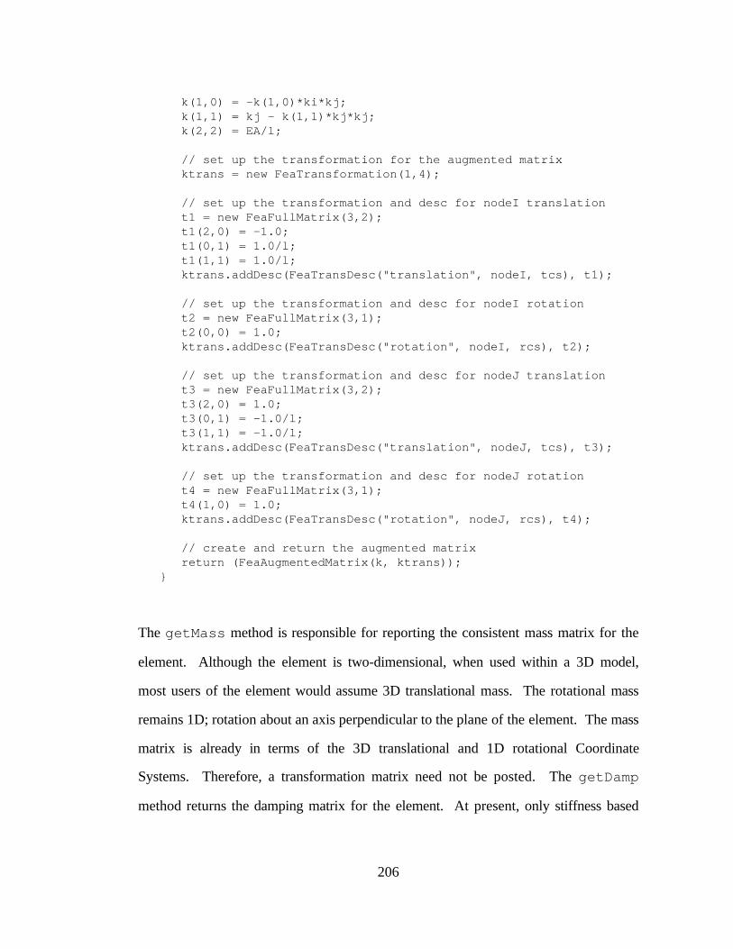
k(1,0) = -k(1,0)*ki*kj;k(1,1) = kj - k(1,1)*kj*kj;k(2,2) = EA/l;
// set up the transformation for the augmented matrixktrans = new FeaTransformation(1,4);
// set up the transformation and desc for nodeI translationt1 = new FeaFullMatrix(3,2);t1(2,0) = -1.0;t1(0,1) = 1.0/l;t1(1,1) = 1.0/l;ktrans.addDesc(FeaTransDesc("translation", nodeI, tcs), t1);
// set up the transformation and desc for nodeI rotationt2 = new FeaFullMatrix(3,1);t2(0,0) = 1.0;ktrans.addDesc(FeaTransDesc("rotation", nodeI, rcs), t2);
// set up the transformation and desc for nodeJ translationt3 = new FeaFullMatrix(3,2);t3(2,0) = 1.0;t3(0,1) = -1.0/l;t3(1,1) = -1.0/l;ktrans.addDesc(FeaTransDesc("translation", nodeJ, tcs), t3);
// set up the transformation and desc for nodeJ rotationt4 = new FeaFullMatrix(3,1);t4(1,0) = 1.0;ktrans.addDesc(FeaTransDesc("rotation", nodeJ, rcs), t4);
// create and return the augmented matrixreturn (FeaAugmentedMatrix(k, ktrans));
}
The getMass method is responsible for reporting the consistent mass matrix for the
element. Although the element is two-dimensional, when used within a 3D model,
most users of the element would assume 3D translational mass. The rotational mass
remains 1D; rotation about an axis perpendicular to the plane of the element. The mass
matrix is already in terms of the 3D translational and 1D rotational Coordinate
Systems. Therefore, a transformation matrix need not be posted. The getDamp
method returns the damping matrix for the element. At present, only stiffness based
206

damping has been implemented. The method is similar to the getStiff method,
except that the base matrix is multiplied by the stiffness based damping factor.
The updateState method is responsible for updating the state of the element in
accordance with the response values of the connecting Nodes. It must update the state
of the hinges and the internal forces. Because the value of the increment in
deformation at the Nodes may change from state update to state update, the internal
deformation values at the end of the last update are stored in qUpdate (1-5). The
update method must bring the values of qUpdate, into line with the current
increment at the Nodes. While obtaining the new values for qUpdate the hinges may
change stiffness. An event to event scheme is used in the update method to make the
internal and external displacement equal. In general terms, the approach is to obtain
the increment in displacement of the nodes in terms of the external element Coordinate
Systems; convert them to q1 , q2 , q3 ; find the difference from the last update; make a
copy of the Constitutive Models for the hinges; and determine the new values for q4
and q5 by advancing the temporary hinges from event to event until q1-5 are in
agreement. Once the new q values are known, the state of the actual hinges and
internal forces are updated in accordance with the new q's. Finally, the new q's are
stored for the next state update. The implementation for this updateState method
is shown below:
void updateState()// updates the state of the element according to the displacements// at the connecting nodes{
// save the moments and axial forcedouble previousSa = axialMat->getCurrentPlusDeltaS();double previousSi = hingeI->getCurrentPlusDeltaS();double previousSj = hingeJ->getCurrentPlusDeltaS();
// get delta displacements at the nodes
207

d1 = nodeI.getIncV(FeaDofType("translation")).get_rep_in(tcs);r1 = nodeI.getIncV(FeaDofType("rotation")).get_rep_in(rcs);d2 = nodeJ.getIncV(FeaDofType("translation")).get_rep_in(tcs);r2 = nodeJ.getIncV(FeaDofType("rotation")).get_rep_in(rcs);
// convert to rotations and axial dispdouble tq1 = d1(1)/l + r1(0) - d2(1)/l;double tq2 = d1(1)/l + r2(0) - d2(1)/l;double tq3 = d2(0) - d1(0);
// get the increment in q from the last updatedouble q1 = tq1 - q1Update;double q2 = tq2 - q2Update;
// save q4 and q5 from last updatedouble tq4 = q4Update;double tq5 = q5Update;
// make copies of the hingestmpHingeI = hingeI.copy();tmpHingeJ = hingeJ.copy();
// commit the tmp hingestmpHingeI->commit();tmpHingeJ->commit();
// set up for the loopdouble factor = 0.0;double previousRotI = 0.0;double previousRotJ = 0.0;
// proceed through the displacements by event to eventwhile (factor < (1.0 - TOLERANCE)){
// recover internal node rotationsdouble q4 = t00 * q1 + t01 * q2;double q5 = t10 * q1 + t11 * q2;
// add to the tmp values of q4 and q5 from last updatetq4 += q4;tq5 += q5;
// calculate the change in hinge rotation and axial straindouble deltaRotI = tq4 - tq1 - previousRotI;double deltaRotJ = tq2 - tq5 - previousRotJ;
// get the event factors for these new increments in rotdouble fi = tmpHingeI->getEventFactorIncV(deltaRotI);double fj = tmpHingeJ->getEventFactorIncV(deltaRotJ);
// get minimum event factorfactor = fi;
208

if ( fj < factor ) factor = fj;
// scale displacements by the event factorpreviousRotI += deltaRotI*factor;previousRotJ += deltaRotJ*factor;deltaRotI *= (factor);deltaRotJ *= (factor);q1 *= (1.0-factor);q2 *= (1.0-factor);tq4 -= q4*(1.0-factor);tq5 -= q5*(1.0-factor);
// update and commit the temporary hingestmpHingeI.setIncV(deltaRotI);tmpHingeJ.setIncV(deltaRotJ);tmpHingeI.commit();tmpHingeJ.commit();
// update the real hingeshingeI.setIncV(previousRotI);hingeJ.setIncV(previousRotJ);
// update the transformationsetT();
}
// calc the inc in axial strain and update the const. modeldouble deltaAxialStrain = tq3/l;axialMat.setIncV(deltaAxialStrain);
// calc the increment in internal forcesbFi = hingeI.getCurrentPlusDeltaS() - previousSi;bFj = hingeJ.getCurrentPlusDeltaS() - previousSj;bFa = (axialMat.getCurrentPlusDeltaS() - previousSa) * area;
// update the internal forcesinternalForceI += bFi;internalForceJ += bFj;axialForce += bFa;
// save the displacements for the next iterationq1Update = tq1;q2Update = tq2;q3Update = tq3;q4Update = tq4;q5Update = tq5;
}
209

The commit method is responsible for committing the state of the element in
accordance with the total current responses at the connecting Nodes. It is important to
note that the commit method may be called after the update method (as is the case for
Newton-Raphson iteration for the model), or on its own (as is the case for event to
event). In either case, the current linearization of the element is still valid. There is no
change in stiffness of the hinges. Therefore, the iteration scheme employed in the
updateState method is not necessary. The element obtains the current total
displacement of the Nodes; converts it in accordance with the external element
Coordinate Systems; forms the change in q1 , q2 , and q3 ; recovers q4 and q5 from
the current t matrix; commits the hinge state; and updates the internal force. To
determine the change in q values from the last committed state, q(1-5)commit are
stored and updated. The implementation for the commit method is shown below.
void commitState(){
// get total displacements at the nodesd1 = nodeI.getTotalV("translation").get_rep_in(tcs);r1 = nodeI.getTotalV("rotation").get_rep_in(rcs);d2 = nodeJ.getTotalV("translation").get_rep_in(tcs);r2 = nodeJ.getTotalV("rotation").get_rep_in(rcs);
// convert to rotations and axial dispdouble tq1 = d1(1)/l + r1(0) - d2(1)/l;double tq2 = d1(1)/l + r2(0) - d2(1)/l;double tq3 = d2(0) - d1(0);
// get inc in rotations since last commit or updatedouble q1 = tq1 - q1Commit - q1Update;double q2 = tq2 - q2Commit - q2Update;
// get delta in disp (from last commit)double dq1 = tq1 - q1Commit;double dq2 = tq2 - q2Commit;double dq3 = tq3 - q3Commit;
// save the total disp for possible next commitq1Commit = tq1;q2Commit = tq2;q3Commit = tq3;
210
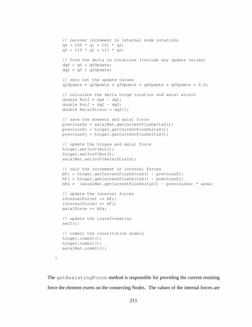
// recover increment in internal node rotationsq4 = t00 * q1 + t01 * q2;q5 = t10 * q1 + t11 * q2;
// form the delta in rotations (include any update values)dq4 = q4 + q4Update;dq5 = q5 + q5Update;
// zero out the update valuesq1Update = q2Update = q3Update = q4Update = q5Update = 0.0;
// calculate the delta hinge rotation and axial straindouble RotI = dq4 - dq1;double RotJ = dq2 - dq5;double AxialStrain = dq3/l;
// save the moments and axial forcepreviousSa = axialMat.getCurrentPlusDeltaS();previousSi = hingeI.getCurrentPlusDeltaS();previousSj = hingeJ.getCurrentPlusDeltaS();
// update the hinges and axial forcehingeI.setIncV(RotI);hingeJ.setIncV(RotJ);axialMat.setIncV(AxialStrain);
// calc the increment in internal forcesbFi = hingeI.getCurrentPlusDeltaS() - previousSi;bFj = hingeJ.getCurrentPlusDeltaS() - previousSj;bFa = (axialMat.getCurrentPlusDeltaS() - previousSa) * area;
// update the internal forcesinternalForceI += bFi;internalForceJ += bFj;axialForce += bFa;
// update the transformationsetT();
// commit the constitutive modelshingeI.commit();hingeJ.commit();axialMat.commit();
}
The getResistingForce method is responsible for providing the current resisting
force the element exerts on the connecting Nodes. The values of the internal forces are
211

maintained by the updateState and commit methods. The
getResistingForce method must communicate these values as an Augmented
Vector object. The Augmented Vector holds the base force vector, a transformation
matrix, and the Coordinate Systems in which the resulting forces are represented. The
transformation matrix and Coordinate Systems are the same as those in the getStiff
method. The base vector ld is given as:
ld = −−
L
N
MMM
O
Q
PPP
intForceI
intForceJ
axialForce
The implementation for the getResistingForce method is shown below:
FeaAugmentedVector& getResistingForce()// return the resisting force of the element as an augmented// vector{
// create the internal force vectorld = new FeaFullVector(3);ld(0) = internalForceI;ld(1) = -internalForceJ;ld(2) = -axialForce;
// set up the transformation for the augmented vectorktrans = new FeaTransformation(1,4);
// set up the transformation and desc for nodeI translationt1 = new FeaFullMatrix(3,2);t1(2,0) = -1.0;t1(0,1) = 1.0/l;t1(1,1) = 1.0/l;ktrans.addDesc(FeaTransDesc("translation", nodeI, tcs), t1);
// set up the transformation and desc for nodeI rotationt2 = new FeaFullMatrix(3,1);t2(0,0) = 1.0;ktrans.addDesc(FeaTransDesc("rotation", nodeI, rcs), t2);
// set up the transformation and desc for nodeJ translationt3 = new FeaFullMatrix(3,2);t3(2,0) = 1.0;
212

t3(0,1) = -1.0/l;t3(1,1) = -1.0/l;ktrans.addDesc(FeaTransDesc("translation", nodeJ, tcs), t3);
// set up the transformation and desc for nodeJ rotationt4 = new FeaFullMatrix(3,1);t4(1,0) = 1.0;ktrans.addDesc(FeaTransDesc("rotation", nodeJ, rcs), t4);
// create and return the augmented matrixreturn (new FeaAugmentedVector(ld, ktrans));
}
The getEventFactor method is responsible for returning the event factor for the
current increment in response at the connecting Nodes. The method does not change
the state of the element in the process. The event factor returned is the smaller of the
event factors for the two hinges. The current increment in displacement is obtained in
terms of the external element Coordinate Systems; this is converted to q1 , q2, and
q3 values; q4 and q5 are recovered using the current t matrix; the increment in
rotation of the hinges is found; the hinges are asked for their event factor for the
increments in rotation; and, finally, the smaller of the two values is returned. The
instance variables of the element are not disturbed. The state of the element is
unaffected as long as the Constitutive Model objects for the hinges do not change their
state when asked to provide their event factor.
double getEventFactor()// returns the minimum event factor based on the state of the// nodes{
// get delta displacements at the nodesd1 = nodeI.getIncV(FeaDofType("translation")).get_rep_in(tcs);r1 = nodeI.getIncV(FeaDofType("rotation")).get_rep_in(rcs);d2 = nodeJ.getIncV(FeaDofType("translation")).get_rep_in(tcs);r2 = nodeJ.getIncV(FeaDofType("rotation")).get_rep_in(rcs);
// convert to rotations and axial dispq1 = d1(1)/l + r1(0) - d2(1)/l;q2 = d1(1)/l + r2(0) - d2(1)/l;q3 = d2(0) - d1(0);
213

// recover internal node rotationsq4 = t00 * q1 + t01 * q2;q5 = t10 * q1 + t11 * q2;
// calculate the change in hinge rotation and axial straindeltaRotI = q4 - q1;deltaRotJ = q2 - q5;deltaAxialStrain = q3/l;
// get the event factors from the constitutive modelsfi = hingeI->getEventFactorIncV(deltaRotI);fj = hingeJ->getEventFactorIncV(deltaRotJ);fa = axialMat->getEventFactorIncV(deltaAxialStrain);
// get the minimum event factor and return itfactor = 1.0;if ( fi < factor ) factor = fi;if ( fj < factor ) factor = fj;if ( fa < factor ) factor = fa;return factor;
}
The setT method is used by the constructors, updateState , commitState
methods. It is responsible for creating the trans instance variable, which is used to
recover the internal rotations (∆ ∆q q4 5 and ) from the external (∆ ∆q q1 2 and ). It is
defined from the following relationship shown previously in this section:
∆∆
∆∆
q
qk
q
q4
5
1 1
2
L
NM
O
QP =
L
NM
O
QP
− k
ki
j
The implementation for the setT method is shown below:
void setT()// set up the transformation between the 5 internal and// the 3 external dof// only set up for q4 and q5 from r1 and r2{
// get the current hinge stiffnesseski = hingeI->getK();kj = hingeJ->getK();
214

// set up kii (place in t for now)t00 = 4.0*EI/l + ki;t01 = 2.0*EI/l;t10 = 2.0*EI/l;t11 = 4.0*EI/l + kj;
// invert kiidet = t00 * t11 - t10 * t01;dum = t00 / det;t00 = t11/det;t01 = -t01/det;t10 = -t10/det;t11 = dum;
// solve for the transformationt00 *= ki;t01 *= kj;t10 *= ki;t11 *= kj;
}
6.4 Building a Model
This section describes the process involved in building a Model through the use of the
constructors for the component classes of the Model. Although it is possible to use the
constructors directly in this manner to build the Model, this is not the intention. A
preprocessor language could translate modeling commands into constructors for the
classes. This language is outside of the scope of the study. The sample model is
shown below.
215

x
z
Node 3
Element 2
Node 2
44
5
3
Load
Node 1
Node 4
y
Element 1
Element 3EA = 1000
Figure 6.4 Sample Model
The first task is the creation of the FeaModel object that will hold the components of
the Model. It is created with the following text, which names the Model as
"TrussModel ":
// ModelFeaModel sub1("TrussModel");
The four Nodes for the Model are defined next. To aid in this, a vector of length 3 is
defined. Each Node is defined in four steps: first the ordinates of the position of the
Node are entered into the vector; the node is then defined by giving it a name and
defining the point in space it occupies (using the vector); 3 degrees of freedom are
added to the Node using the addDof method with a name for the degrees of freedom
and a Coordinate System; finally, the Node is added to the Model using the
addDofGroup method of the Model. This is repeated for all four Nodes.
// NodesFeaFullVector tmpv(3);
tmpv(0) = 0.0; tmpv(1) = 0.0; tmpv(2) = 0.0;FeaNode node1("nodeOne", FeaGeoPoint(tmpv, Fea3DRect()));node1.addDof("translation", Fea3DRect());sub1.addDofGroup(node1);
216

tmpv(0) = 4.0; tmpv(1) = 0.0; tmpv(2) = 3.0;FeaNode node2("nodeTwo", FeaGeoPoint(tmpv, Fea3DRect()));node2.addDof("translation", Fea3DRect());sub1.addDofGroup(node2);
tmpv(0) = 4.0; tmpv(1) = 0.0; tmpv(2) = 0.0;FeaNode node3("nodeThree", FeaGeoPoint(tmpv, Fea3DRect()));node3.addDof("translation", Fea3DRect());sub1.addDofGroup(node3);
tmpv(0) = 4.0; tmpv(1) = 5.0; tmpv(2) = 0.0;FeaNode node4("nodeFour", FeaGeoPoint(tmpv, Fea3DRect()));node4.addDof("translation", Fea3DRect());sub1.addDofGroup(node4);
Constraints are added to the model by defining an equation of constraint. In this
example, the X and Z displacements of Node 1, and the X, Y, and Z displacements of
Nodes 3 and 4, are treated as constraints. The Y displacement of Node 1 is treated as
a Boundary Condition with Prescribed Values. For these simple constraints in this
example, each equation involves only one degree of freedom component. The
component is described by a FeaDofCompDesc object, which is formed by defining the
type of movement, the Node, and the coordinate axis number for the direction. The
equation is represented by a dictionary of pairs of FeaDofCompDesc objects and the
associated value for its coefficient in the equation. The values in this example are set to
unity; any value will do. Each equation of constraint is then added to the model using
the addConstraint method.
// Constraintsdictionary<FeaDofCompDesc&, double> c1, ... c8;
c1[FeaDofCompDesc("translation", node1, 1)] = 1.0;sub1.addConstraint(FeaConstraint(c1));c2[FeaDofCompDesc("translation", node1, 3)] = 1.0;sub1.addConstraint(FeaConstraint(c2));
c3[FeaDofCompDesc("translation", node3, 1)] = 1.0;sub1.addConstraint(FeaConstraint(c3));c4[FeaDofCompDesc("translation", node3, 2)] = 1.0;
217

sub1.addConstraint(FeaConstraint(c4));c5[FeaDofCompDesc("translation", node3, 3)] = 1.0;sub1.addConstraint(FeaConstraint(c5));
c6[FeaDofCompDesc("translation", node4, 1)] = 1.0;sub1.addConstraint(FeaConstraint(c6));c7[FeaDofCompDesc("translation", node4, 2)] = 1.0;sub1.addConstraint(FeaConstraint(c7));c8[FeaDofCompDesc("translation", node4, 3)] = 1.0;sub1.addConstraint(FeaConstraint(c8));
Boundary conditions are added to the model by defining the FeaDofCompDesc for the
degree of freedom component as above. The FeaDofCompDesc object is added to the
Model using the addPrescBC method.
// Boundary ConditionFeaDofCompDesc bc("translation", node1, 2);sub1.addPrescBC(bc);
The next step is to define the Elements in the problem. In order to do this, Constitutive
Models for the Elements must be defined. In this example, a linear elastic 1D
stress/strain Constitutive Model and a bi-linear elastic 1D stress/strain Constitutive
Model are required. They are both defined by indicating the material, A36 Steel, with
which the Constitutive Models will be calibrated.
// Constitutive ModelFea1DStressStrainLinearElastic mat(FeaA36Steel());Fea1DStressStrainBiLinearElastic matB(FeaA36Steel());
The three Truss Bar Elements are defined by giving them a name, cross sectional area,
the two Nodes to which they connect, and a Constitutive Model. The Elements are
added to the model using the addElement method.
// ElementsFeaTrussBar el1("element1", 1.0e3, node1, node2, matB);
218

sub1.addElement(el1);
FeaTrussBar el2("element2", 1.0e3, node2, node3, mat);sub1.addElement(el2);
FeaTrussBar el3("element3", 1.0e3, node2, node4, mat);sub1.addElement(el3);
The final portion of the model definition is to define the Loads which will act upon the
Model. First a Load Case is defined by providing a name. The components of the
Load Case will then be built and added.
// Load CaseFeaLoadCase lc1("loadCase1");
A Time Function must be provided for the time varying loads. Data points are added
to the function using the addTimeAndValue method with the time and function
values as the arguments.
// Time FunctionFeaTimeFunction tf;tf.addTimeAndValue(0.00, 1.0);tf.addTimeAndValue(0.02, 1.0);
Prescribed Displacement values relating to the Boundary Conditions in the Model are
defined by a FeaDofCompDesc object, the base displacement value, and a time function.
The Prescribed Displacement is added to the Load Case using the addPresDisp
method.
// Pres DispFeaPresDisp node1pd(bc, 0.0, tf);lc1.addPresDisp(node1pd);
219

Nodal loads are defined by the Node to which they apply, the type of degree of
freedom, a vector for the load, and a time function. The vector for the load is defined
by a FeaGeoVector object which is constructed from the ordinates and the Coordinate
System in which the ordinates are defined. The Nodal Loads are added to the Load
Case using the addLoad method.
// Node LoadFeaFullVector tmpv2(3);tmpv2(0) = 10.0;FeaGeoVector vec(tmpv2, Fea3DRect());FeaVectorLoad vl(node2, "translation", vec, tf);lc1.addLoad(vl);
Finally, the Load Case itself is added to the model using the addLoadCase method.
sub1.addLoadCase(lc1);
6.5 Using the Finite Element Program
This section describes the use of several of the analysis types implemented in the finite
element program: linear static analysis; nonlinear static event to event analysis;
nonlinear static analysis with Newton-Raphson iteration; and nonlinear dynamic
analysis with Newton-Raphson iteration. At present, the analysis is directed by adding
C++ code directly to the program. This is obviously not a permanent solution. When
an input language for the program is defined, it will include a means to direct the
analysis. As will be seen, the amount of code that is required to direct the analysis is
only a few lines. Also, the code for the various analysis types differs only slightly.
220

6.5.1 Linear Static Analysis
To demonstrate the use of the linear static analysis, the FeaLinearStaticAnalysis class is
applied to the frame shown in Figure 6.5.1. The frame is from the Holiday Inn building
in Van Nuys California. It is a seven-story reinforced concrete structure which
experienced significant distress during the Northridge earthquake in 1994. The
structure properties are detailed in the literature [23].
A A
SECTION A-A VIEW
PLAN VIEW
Figure 6.5.1 Sample Problem: Holiday Inn, Van Nuys, Exterior Frame. Ref. [23]
221

The planar model for an exterior frame consists of 72 nodes and 119 elements, and
represents a typical real world analysis problem. The nodes each have two
translational, and one rotational degree of freedom, for a total of 216 degrees of
freedom. The elements are modeled as beam-columns with elastic-plastic rotational
hinges at each end based on the properties of the reinforced concrete cross section.
The load applied to the structure is a triangularly distributed, lateral load based on the
structure mass. This type of loading is typically used for a nonlinear push-over analysis.
In this case, only a linear structure response is considered, but the nonlinear response is
considered in the next section.
The actual code for the linear analysis is shown below:
FeaLinearStaticAnalysis analysis(model);analysis.init("loadCase1");analysis.analyze();outputNodesAndElements();
The analysis object is constructed by specifying the model to be analyzed. The analysis
is then initialized with the load case, and the analysis is performed. The state of the
Nodes and Elements is printed for each step using the method
outputNodesAndElements , which is defined along with the Model.
6.5.2 Nonlinear Static Analysis
To demonstrate the use of the nonlinear static analysis classes, the sample problem of
the exterior frame from the Holiday Inn, Van Nuys building from the previous section
is reused. To perform the analysis, both an event to event and a Newton-Raphson
222

analysis object are used. Again, the load applied to the structure is a triangularly
distributed, lateral load based on the structure mass.
The code for the event to event analysis is:
FeaEventToEventStaticAnalysis analysis(model);analysis.init("loadCase1");for ( double lsf = 0.0; lsf < 1.0; lsf += 0.005){
analysis.analyze(lsf );cout << "Load Step Factor = " << lsf << "\n";outputNodesAndElement();
}
The analysis object is constructed by specifying the model to be analyzed. The analysis
is then initialized with the load case. Although the load is static, a time function is
defined for the loads and used to represent the load step factor. The function specifies
a loading of 1.0 at a step factor of 1.0. A loop is set up in which the value of the load
step factor is incremented by 0.005. Inside the loop, the analysis is directed by the
analyze method with the load case and the current value of the load step factor
given as the arguments. The state of the Nodes and Elements is printed for each step
using the method outputNodesAndElements , which is defined along with the
Model.
The code for the Newton-Raphson iteration scheme is identical to that of the event to
event type, but the analysis class selected is FeaNRStaticAnalysis instead of
FeaEventToEventStaticAnalysis. The code that directs the nonlinear static analysis with
Newton-Raphson iteration is:
FeaNRStaticAnalysis analysis(model);analysis.init("loadCase1");
223

for ( double lsf = 0.0; lsf < 1.0; lsf += 0.005){
analysis.analyze(lsf );cout << "Load Step Factor = " << lsf << "\n";outputNodesAndElement();
}
The resulting top floor lateral displacement is shown in Figure 6.5.2a.
Top Floor Displacement (in)
Load
Ste
p F
acto
r
0
0.05
0.1
0.15
0.2
0.25
0 1 2 3 4 5 6 7
Figure 6.5.2a Top Floor Displacement
The calculated moments in the exterior ground floor column are plotted in Figure
6.5.2b.
224

Load Step Factor
Col
umn
Mom
ent (
k-in
)
0
1000
2000
3000
4000
5000
0 0.05 0.1 0.15 0.2 0.25
Mbase
Mtop
Figure 6.5.2b Exterior Ground Floor Column End Moments
6.5.3 Nonlinear Dynamic Analysis
As a demonstration of dynamic analysis, the FeaNRDynamicAnalysis class is used to
perform a nonlinear analysis, using Newton-Raphson iteration on the following
example:
Column Data:
E = 29,000 ksi
A = 324 in
I = 1593.1 in
2
4
M k inp = 2400 h = 120
l =180
nodal masskip s
in= 8 127
2
.
P = 60 kips
Figure 6.5.3a Sample Problem
225

The structure is given Rayleigh damping ratios of βk = 0 0056. and βm = 0 4. , to
provide for 5% damping. The loading is constant. The beam is assumed to be near
rigid. The right side column is linear, the left side contains elastic-perfectly-plastic
hinges that yield at Mp = 2400 kip-in.
For comparison, the structure is analyzed for both the nonlinear case and the linear case
(Mp is raised above the demand moment). The code directing the analysis is shown
below:
FeaNRDynamicAnalysis analysis(model, 0.0056, 0.4);analysis.init("loadCase1");for ( double time = 0.1; time <= 10.01; time += 0.1){
analysis.analyze(time);cout << "\nTime = " << time << '\n';node1.print();node2.print();node3.print();el1.print();el2.print();el3.print();
}
The analysis object is constructed by specifying the model and the two damping ratios.
The analysis is then initialized with the load case, and the starting time of zero. A loop
is set up in which the value of time is incremented by 0.1s. Inside the loop, the analysis
is directed by the analyze method, with the load case and the current value of time
given as the arguments. The state of the nodes and elements is printed for each step.
The resulting floor displacement and column moments are plotted in Figures 6.5.3a and
6.5.3b, respectively. In Figure 6.5.3b, the column moments for the linear case are
226

identical. In the nonlinear case, Mleft refers to the moment at the base of the left-hand
column, and Mright refers to the moment of the right-hand column.
Time (s)
Dis
plac
emen
t (in
)
0
0.05
0.1
0.15
0.2
0.25
0.3
0.35
0.4
0 1 2 3 4 5 6 7 8 9 10
Linear
NonLinear
Figure 6.5.3b Top Floor Displacement
Time (s)
Mom
ent (
k in
)
0
500
1000
1500
2000
2500
3000
3500
4000
0 1 2 3 4 5 6 7 8 9 10
Linear
Nonlinear (Mleft)
Nonlinear (Mright)
Figure 6.5.3c Column Moments
227

As is expected for the linear case, the displacements oscillate (Figure 6.5.3b),
eventually settling on the static displacement as the structure damping eliminates the
motion. For the nonlinear case, the plastic moment capacity for the left column is
exceeded. Therefore, the displacements are higher. The final displacement is also
higher than for the linear case, due to the plastic rotation of the hinge.
The left and right column moments are identical (Figure 6.5.3c) for the linear case. As
the damping takes over and the oscillations stop, the moments settle to the static
values. For the nonlinear case, the moment in the left column, Mleft, is capped at the
plastic moment capacity.
228

7. Conclusions and Future Work
7.1 Conclusions
A new object-oriented design for a finite element program has been presented. The
design was implemented in the C++ programming language. The program is flexible,
extendible, and easily modified for a variety of finite element analysis procedures. The
problems inherent in existing procedural based finite element programs are eliminated
by design. To modify or extend the program, the required knowledge of the
components is restricted to the public interfaces of the classes. The reuse of code is
promoted by the use of inheritance. The effect of a change to the data structures is
limited to the class that owns the data; there is no ripple effect through the program.
Dependencies between components of the design are explicitly defined and are easily
determined from the public interfaces of the classes. The integrity of the program's
data structures is enforced by the encapsulation features of the implementation
language.
229

7.1.1 Architecture
The principal feature of the software architecture is the Map object. The Map isolates
the degree of freedom based information in the Model from the governing equation
information in the Analysis. It is this isolation that limits the degree of knowledge
required to work on a component of the system, and provides the flexibility in
applications. As a result of the Map, writers of Analysis objects do not need details of
the Model and can focus on the numerical algorithms. Also, elements can be
formulated with reference to any convenient coordinate system; the Map handles the
transformations. Finally, the orientation of the degrees of freedom can vary. The Map
makes no assumptions as to the coordinate systems used at the nodes.
The architecture includes three Handlers, each designed to perform tasks that are
common to most analysis methods. This greatly reduces the workload of the Analysis
object authors. The Handlers are: the Constraint Handler, which processes the
constraints; the Reorder Handler, which reorders the equations of equilibrium for
efficiency; and the Matrix Handler, which constructs the matrices and vectors used by
the Analysis to hold the system properties. The Handlers not only isolate their tasks
from the rest of the system, they encourage the reuse of significant amounts of code.
Writers of Analysis objects simply choose from the existing set of Handlers or add a
new Handler to the library for all to use.
The Constraint Handler permits the inclusion of the multi-point constraints. The
manner in which the constraints are to be processed (by transformations, penalty
230

functions, Lagrangian multipliers, etc.) can be chosen by the Analysis object. This
gives the Analysis writer the flexibility to choose the most appropriate type.
Since the constraints are applied before the renumbering scheme is invoked, the
Reorder object can optimize the equation of equilibrium numbering including the
effects of constraints. The Reorder object is written for use with a specific type of
Constraint Handler. Thus, it is sensitive to the ordering requirements unique to the
method of constraint processing.
A Matrix Handler is required for each type of matrix used by an Analysis object. The
selection of a type of Matrix Handler is the only manner in which the Analysis object
indicates the type of matrix it will use for the system properties.
The enforcement of the semantics of update, commit, and event factor throughout the
system provides a uniform interface for the Analysis writer. An update describes a new
increment from the last committed state of the Model. The combination of the last
committed state and the current increment describes the current total state. The Map
updates the state of the Model according to the responses the Analysis provides. All
subsequent requests for system properties from the Map will be according to the
current total state. A commit implies that the total state becomes the new committed
state, and the increment in state is set to zero. An Analysis may iterate through many
total states, but commits only those that are on the desired solution path. An event
factor is the proportion of the increment in state a component of the Model can
accommodate without violating the assumptions of its linearization.
231

In contrast with most finite element analysis programs, element loads are computed in
the resisting force calculation and not treated as equivalent nodal loads. This is an
advantage in nonlinear analysis, as the distribution of the element loads to the nodes
may change as the element experiences nonlinear behavior. Provision for the traditional
approach is also provided.
7.1.2 Ease of Modification and Extendibility
The program is easily modified. The ease of modification is due to the object-oriented
principals of abstraction, encapsulation, inheritance, and polymorphism. The essential
properties of an object form the abstraction for the class. The abstraction is enforced
by the implementation language through the encapsulation of the private data of the
object and the private implementation of the publicly available services the class
provides to the system. The class alone has access to its specific implementation of the
public services and its private data Classes are related by an inheritance hierarchy. A
subclass inherits the public appearance of the superclass. The classes are polymorphic;
any subclass can be used in the place of a superclass.
Since the instance variables for an object are encapsulated in the class definition, they
can be freely modified without affecting other objects. In both the initial development
and subsequent refinements of a class, the programmer may change the class's data.
The private implementation of the public methods can be modified without any external
effect. The portion of the implementation that is fixed are the method names,
arguments, and return data types in the public interfaces presented in the Appendix.
232

Polymorphism eases program modification. The type of matrix used for the system
property matrices in the Analysis objects is modified by simply changing the definition
of the type of Matrix Handler used. Also, the type of constitutive model used in an
element is modified by simply specifying the new type in the creation of the element.
The element's code is unchanged.
Several classes were added to the basic system as a demonstration of the extendibility
of the program. These classes were: a two-dimensional beam element with hinges at
the ends; a two-dimensional rectangular coordinate system; a moment-rotation elastic
perfectly plastic constitutive model; a super-element/substructure class using the
element interface; and several analysis classes including a nonlinear dynamic solution
scheme using Newton-Raphson iteration. The objects were easily incorporated into the
system. Of particular interest is that these extensions included both new code using the
old, as is the case of a new Analysis object using the methods of the Map, and the old
code using the new, such as the Map object using the new two-dimensional rectangular
coordinate system to transform the system property objects. In both cases the existing
code remains unchanged.
7.2 Future Work
The future work envisioned for the finite element analysis program is broken down into
the following tasks:
1. Numerical Object Library: A library of numerical objects must be selected. For
the sake of furthering research, it is desirable to choose one that is publicly
233

available. A likely candidate is LAPACK++ [13]. Regardless of the choice, an
interface between the library and the finite element program will have to be written
to minimize the dependency on the specific library. For each matrix type used by
the Analysis, a Matrix Handler object that creates instances of the matrix must be
written. Also, an assemble method must be included. In addition to the typical
matrices used in finite element analysis (regular, symmetric, diagonal, symmetric
banded, and symmetric profile), a key component of the numerical library will be
the block matrix object. This matrix type is generally not included in numerical
libraries and will have to be added. The blocks will consist of matrix types
provided by the library. The block matrix object must take advantage of zero, and
identity matrix blocks in both the data storage and multiply methods. For
efficiency, the two crucial methods for the block matrix object are: the multiply
method for two block matrices, and a triple product method for BtAB, where B is a
block matrix and A is a regular matrix (likely symmetric).
2. Container Class Library: The choice of container class library should be
reviewed. The ANSI/ISO C++ Standard Committee has voted to make the
Standard Template Library (STL) [36] part of the standard C++ library. The STL
contains the necessary data structures, and will be included in the next revision to
the finite element program.
3. Extensions: Constraint Handlers and Analysis objects using the method of
Lagrangian multipliers and penalty functions to process the constraints are needed.
A typical Reorder Handler using a reverse Cuthill-McKee [12] algorithm should be
developed. Extension of the geometric objects to include higher order tensors may
prove useful to some authors of Element objects.
234

4. Input and Output: A preprocessor language is required that will translate
modeling commands into constructors for the classes. A post-processor for the
output is also required.
5. Implementation Language: The choice of C++ as an implementation language
should be reviewed. Although it is by far the most popular object-oriented
language available, it is not necessarily the best. The syntax is awkward, the
memory management scheme places too much emphasis on the programmer, and
the dynamic binding of methods is restrictive.
235

References
1. Adeli H.; Yu G., An Integrated Computing Environment for Solution of ComplexEngineering Problems Using the Object-Oriented Programming Paradigm and aBlackboard Architecture, Computers & Structures, Vol. 54, No. 2, 255-265,1995.
2. Anderson E.; Bai Z.; Bischof C.; Demmel J.; Dongarra J.; Du Croz J.; GreenbaumA.; Hammarling S.; McKenney A.; Ostrouchov S.; Sorensen D., LAPACKUser's Guide. SIAM Publications, Philadelphia, 1992.
3. Baugh J. W., Rehak D. R., Computational Abstractions For Finite ElementProgramming. Technical Report R-89-182 Department Of Civil Engineering,Carnegie Institute Of Technology
4. Baugh J. W.; Rehak D. R., Data Abstraction in Engineering Software Development,Journal of Computing in Civil Engineering, Vol. 6, No. 3, July, 1992.
5. Beaufait F.; Rowan W.; Hoadley P.; Hackett R., Computer Methods of StructuralAnalysis. Prentice-Hall, New Jersey, 1970.
6. Budd T., Classic Data Structures in C++. Addison-Wesley, New York, 1994.
7. Chen W. F.; Sotelino E. D.; White D. W., High Performance Computing In CivilEngineering Applications [West Lafayette, Ind. School Of Engineering, PurdueUniversity, 1990].
236

8. Chudoba R.; Bittnar Z.; Krysl P., Explicit Finite Element Computation: An Object-Oriented Approach. Computing in Civil and Building Engineering, Rotterdam,1995.
9. Cline M.; Lomow G., C++ FAQs. Addison-Wesley, New York, 1995.
10. Clough R.; Penzien J., Dynamics of Structures. McGraw Hill, New York, 1975.
11. Cook R.; Malkus D.; Plesha M., Concepts and Applications of Finite ElementAnalysis, Third Edition. John Wiley & Sons, New York, 1989.
12. Cuthill E.; McKee J., Reducing the bandwidth of sparse symmetric matrices. In:Proceedings of the 24th Natrional Conference of the ACM, Associtation forComputing Machinery, 1969.
13. Dongarra J. J.; Pozo R.; Walker D. W., LAPACK++: A Design Overview ofObject-Oriented Extensions for High Performance Linear Algebra, ACM 0-8186-4340-4/93/0011, 1993.
14. Duboispelerin Y.; Zimmermann T., Object-Oriented Finite Element Programming.3. An Efficient Implementation In C++. Computer Methods In AppliedMechanics And Engineering, 1993 Sept., V108 N1-2:165-183.
15. Duboispelerin Y.; Zimmermann T.; Bomme P., Object-Oriented Finite ElementProgramming .2. A Prototype Program In Smalltalk. Computer Methods InApplied Mechanics And Engineering, 1992 Aug., V98, N3:361-397.
16. Ellis M.; Stroustrup B., The Annotated C++ Reference Manual. Addison-Wesley,New York, 1990.
17. Fenves G. L., Object-Oriented Programming For Engineering SoftwareDevelopment. Engineering With Computers, 1990 Winter, V6 N1:1-15.
18. Filho J. S. R. A.; Devloo P. R. B., Object-Oriented Programming in ScientificComputations: The Beginning of a New Era. Engineering Computations, Vol.8, 81-87, 1991.
19. Forde B. W. R.; Foschi R. O.; Stiemer S. F., Object-Oriented Finite ElementAnalysis. Computers & Structures, 1990, V34 N3:355-374.
20. Hoffmeister P.; Zahlten W.; Kratzig W. B., Object-Oriented Finite ElementModeling. Second Congress on Computing in Civil Engineering, ASCE, 1994.
21. Humar J., Dynamics of Structures. Prentice Hall, New Jersey, 1990.
237

22. Lu J.; White D. W.; Chen W. F.; Dunsmore H. E., A Matrix Class Library in C++For Structural Engineering Computing, Computers & Structures, Vol. 55, No.1, 95-111, 1995.
23. Lynn A.; Moehle J.; Whittaker A., Evaluation of Existing, Seven-story, ReinforcedConcrete Building. Senventh U. S. - Japan Workshop on Improvement ofStructural Design and Construction Practices, Lessons Learned from Kobe andNorthridge. Kobe, 1996.
24. Mackie R. I., Object-Oriented Programming Of The Finite Element Method.International Journal For Numerical Methods In Engineering, 1992 Aug. 15,V35 N2:425-436.
25. Menetrey P.; Zimmermann T., Object-Oriented Non-Linear Finite ElementAnalysis - Application To J2 Plasticity. Computers & Structures, 1993 Dec. 3,V49 N5:767-777.
26. Miller G. R., An Object-Oriented Approach To Structural Analysis And Design.Computers & Structures, 1991, V40 N1:75-82.
27. Miller G. R., Coordinate-Free Isoparametric Elements. Computers & Structures,1993 Dec. 17, V49 N6:1027-1035.
28. Miller G. R.; Rucki M. D., A Program Architecture for Interactive NonLinearDynamic Analysis of Structures, Second Congress on Computing in CivilEngineering, ASCE, 1994.
29. Pidaparti R. M. V.; Hudli A. V., Dynamic Analysis of Structures Using Object-Oriented Techniques, Computers & Structures, Vol. 49, No. 1, 149-156, 1993.
30. Raphael B.; Krishnamoorthy C. S., Automating Finite Element Development UsingObject-Oriented Techniques, Engineering Computations, Vol. 10, 267-278,1993.
31. Rihaczek C.; Kroplin B., Object-Oriented Design of Finite Element Software forTransient, Non-Linear Coupling Problems. Second Congress on Computing inCivil Engineering, ASCE, 1994.
32. Robinson J, Integreated Theory of Finite Element Methods. John Wiley & Sons,London, 1973.
33. Rumbaugh J.; Blaha M.; Premerlani W.; Eddy F.; Lorensen W., Object-OrientedModeling and Design. Prentice Hall, New Jersey, 1991.
238

34. Scholz S. P., Elements of an Object-Oriented FEM++ Program in C++, Computers& Structures, Vol. 43, No. 3, 517-529, 1992.
35. Sotelino E. D.; White D. W.; Chen W. F., Domain-Specific Object-OrientedEnvironment For Parallel Computing, Report: Ce-Str-92-41, School Of CivilEngineering, Purdue Univ., West Lafayette, Indiana, [1992]P 30, (Presented AtThe 2nd International Conference On Discrete Element Methods, Mar. 18,1993.)
36. Stepanov A.; Lee M., The Standard Template Library. Hewlett PackardCompany, Oct 1995.
37. Stroustrup B., The C++ Programming Language, Second Edition. Addison-Wesley, New York, 1993.
38. Yu G.; Adeli H., Object-Oriented Finite Element Analysis Using EER Model.Journal Of Structural Engineering-ASCE, 1993 Sept., V119 N9:2763-2781.
39. Zahlten W.; Demmert P.; Kratzig W. B., An Object-Oriented Approach toPhysically Nonlinear Problems in Computational Mechanics. Computing inCivil and Building Engineering, Rotterdam, 1995.
40. Zeglinski G. W.; Han R. P. S.; Aitchison P., Object-Oriented Matrix Classes ForUse In A Finite Element Code Using C++. International Journal For NumericalMethods In Engineering, 1994 Nov. 30, V37 N22:3921-3937.
41. Zhang H.; White D. W.; Chen W. F., A Library For Object-Oriented ProgrammingIn C. [West Lafayette, Ind. : School Of Civil Engineering, Purdue University,1990].
42. Zhang H.; White D. W.; Chen W. F., The SESDE Object Library Manual. [WestLafayette, Ind. : School Of Civil Engineering, Purdue University, 1990].
43. Zhang H.; White D.W.; Chen W. F., An Object-Oriented Matrix ManipulationLibrary [West Lafayette, Ind. : School Of Civil Engineering, PurdueUniversity, 1990].
44. Zienkiewicz O.; Taylor R., The Finite Element Method, Fourth Edition, Volumes 1and 2. McGraw-Hill, London, 1989.
45. Zimmermann T.; Duboispelerin Y.; Bomme P., Object-Oriented Finite ElementProgramming .1. Governing Principles. Computer Methods In AppliedMechanics And Engineering, 1992 Jul., V98, N2:291-303.
239

Appendix: C++ Class Interfaces
class Fea1DConstitutiveModel : public FeaConstitutiveModel {// abstract 1D stress-strain constitutive modelpublic:
// provide a copy of the objectvirtual Fea1DConstitutiveModel& copy() = 0;
// state operationsvirtual void setIncV(double incV) = 0;virtual void setTotalV(double totalV) = 0;virtual void setInitialV(double initialV) = 0;virtual void commit() = 0;virtual double getEventFactorIncV(double incV) = 0;virtual double getEventFactorTotalV(double totalV) = 0;
// provide current propertiesvirtual double getCurrentCommittedS() = 0;virtual double getCurrentPlusDeltaS() = 0;virtual double getK() = 0;
};
class Fea1DBiLinearElastic : public Fea1DConstitutiveModel{// 1D stress-strain bi-linear elastic constitutive modelpublic:
// constructorFea1DBiLinearElastic(FeaMaterial& material);
// provide a copy of the object
240

virtual Fea1DConstitutiveModel& copy() = 0;
// state operationsvirtual void setIncV(double incV) = 0;virtual void setTotalV(double totalV) = 0;virtual void setInitialV(double initialV) = 0;virtual void commit() = 0;virtual double getEventFactorIncV(double incV) = 0;virtual double getEventFactorTotalV(double totalV) = 0;
// provide current propertiesvirtual double getCurrentCommittedS() = 0;virtual double getCurrentPlusDeltaS() = 0;virtual double getK() = 0;
};
class Fea1DLinearElastic : public Fea1DConstitutiveModel{// 1D stress-strain linear elastic constitutive modelpublic:
// constructorFea1DLinearElastic(FeaMaterial& material);
// provide a copy of the objectvirtual Fea1DConstitutiveModel& copy() = 0;
// state operationsvirtual void setIncV(double incV) = 0;virtual void setTotalV(double totalV) = 0;virtual void setInitialV(double initialV) = 0;virtual void commit() = 0;virtual double getEventFactorIncV(double incV) = 0;virtual double getEventFactorTotalV(double totalV) = 0;
// provide current propertiesvirtual double getCurrentCommittedS() = 0;virtual double getCurrentPlusDeltaS() = 0;virtual double getK() = 0;
};
class Fea1DMRotBiLinearElastic : public Fea1DConstitutiveModel{// 1D moment-rotation bi-linear elastic constitutive modelpublic:
// constructorFea1DMRotBiLinearElastic(double stiffness1, double stiffness2,
double Myield);
// provide a copy of the objectvirtual Fea1DConstitutiveModel& copy() = 0;
// state operations
241

virtual void setIncV(double incV) = 0;virtual void setTotalV(double totalV) = 0;virtual void setInitialV(double initialV) = 0;virtual void commit() = 0;virtual double getEventFactorIncV(double incV) = 0;virtual double getEventFactorTotalV(double totalV) = 0;
// provide current propertiesvirtual double getCurrentCommittedS() = 0;virtual double getCurrentPlusDeltaS() = 0;virtual double getK() = 0;
};
class Fea1DMRotElasticPlastic : public Fea1DConstitutiveModel{// 1D moment-rotation elastic perfectly plastic constitutive modelpublic:
// constructorFea1DMRotElasticPlastic(double stiffness1, double Myield);
// provide a copy of the objectvirtual Fea1DConstitutiveModel& copy() = 0;
// state operationsvirtual void setIncV(double incV) = 0;virtual void setTotalV(double totalV) = 0;virtual void setInitialV(double initialV) = 0;virtual void commit() = 0;virtual double getEventFactorIncV(double incV) = 0;virtual double getEventFactorTotalV(double totalV) = 0;
// provide current propertiesvirtual double getCurrentCommittedS() = 0;virtual double getCurrentPlusDeltaS() = 0;virtual double getK() = 0;
};
class Fea1DMRotLinearElastic : public Fea1DConstitutiveModel{// 1D moment-rotation linear elastic constitutive modelpublic:
// constructorFea1DMRotLinearElastic(double stiffness);
// provide a copy of the objectvirtual Fea1DConstitutiveModel& copy() = 0;
// state operationsvirtual void setIncV(double incV) = 0;virtual void setTotalV(double totalV) = 0;virtual void setInitialV(double initialV) = 0;virtual void commit() = 0;
242

virtual double getEventFactorIncV(double incV) = 0;virtual double getEventFactorTotalV(double totalV) = 0;
// provide current propertiesvirtual double getCurrentCommittedS() = 0;virtual double getCurrentPlusDeltaS() = 0;virtual double getK() = 0;
};
class Fea1DRect : public FeaCoOrdSys {// 1D rectangular coordinate systempublic:
// constructorsFea1DRect();Fea1DRect(FeaFullVector& rotation);Fea1DRect(FeaGeoPoint& p1, FeaGeoPoint& p2);
// transformations to and from global 3D rectFeaFullMatrix& get_trans_to(Fea1DRect& other);FeaFullMatrix& trans_to_global();FeaFullMatrix& trans_from_global();
// number of axis in coordinate systemint num_of_axis();
// make a copyFeaCoOrdSys& copy();
};
class Fea2DRect : public FeaCoOrdSys {// 2D rectangular coordinate systempublic:
// constructorsFea2DRect();Fea2DRect(FeaFullVector& rotataions);Fea2DRect(FeaGeoPoint& p1, FeaGeoPoint& p2, FeaGeoPoint& p3);
// transformations to and from global 3D rectFeaFullMatrix& get_trans_to(Fea2DRect& other);FeaFullMatrix& trans_to_global();FeaFullMatrix& trans_from_global();
// number of axis in coordinate systemint num_of_axis();
// make a copyFeaCoOrdSys& copy();
};
243

class Fea3DRect : public FeaCoOrdSys {// 3D rectangular coordinate systempublic:
// constructorsFea3DRect();Fea3DRect(FeaFullVector& rotations);Fea3DRect(FeaGeoPoint& p1, FeaGeoPoint& p2, FeaGeoPoint& p3);
// transformations to and from global 3D rectFeaFullMatrix& get_trans_to(Fea3DRect& other);FeaFullMatrix& trans_to_global();FeaFullMatrix& trans_from_global();
// number of axis in coordinate systemint num_of_axis();
// make a copyFeaCoOrdSys& copy();
};
class FeaA36Steel : public FeaMaterial {// A36 steel materialpublic:
// kip, inch, second, Farenheitdouble youngsModulus() { return 2.9e4; };double coefOfThermalExp() { return 6.5e-6; };double weightDensity() { return 3.403e-3; };double massDensity() { return 8.806e-6; };double yieldStress() { return 36.0; };double postYieldModulus() { return 1.0e-3; };
};
class FeaAugmentedMatrix {// matrix augmented with transformationspublic:
// constructorFeaAugmentedMatrix(FeaFullMatrix& mat, FeaTransformation& trans);
// add a FeaTransformationvoid addT(FeaTransformation& trans);
// return a pointer to the last transFeaTransformation& getLastT();
// return the transformed KFeaFullMatrix& getTransformedK();
// return the id vector for the transformed Kint* getId();
};
244

class FeaAugmentedVector {// vector augmented with transformationspublic:
// constructorFeaAugmentedVector(FeaFullVector& vec, FeaTransformation& trans);
// add a FeaTransformationvoid addT(FeaTransformation& trans);
// return a pointer to the last transFeaTransformation& getLastT();
// return the transformed FeaLoadFeaFullVector& getTransformedLoad();
// return the id vector for the transformed Vectorint* getId();
};
class FeaBlockMatrix : public FeaMatrix {// block matrixpublic:
// constructor// initialize with number of row and column blocksFeaBlockMatrix(int numRowBl,int numColBl);
// print out the matrixvoid print();
// add a block with top left hand absolute cornervoid addBlock(FeaFullMatrix& mat, int row, int col);
// operationsdouble& operator()(int, int);FeaMatrix& operator*(FeaMatrix& other);FeaBlockMatrix& operator*(FeaBlockMatrix& other);FeaBlockMatrix& operator*(FeaFullMatrix& other);FeaFullVector& operator*(FeaFullVector& other);FeaBlockMatrix& operator+=(FeaMatrix& other);FeaFullMatrix& getSubMatrix(int, int, int, int);
// provide a transpose of the matrixFeaBlockMatrix& transpose();
//top left absolute postion and row and column lengthFeaFullMatrix& getBlock00();FeaFullMatrix& getBlock(int, int);
// assemble matrix and given id's
245

void assemble(FeaFullMatrix& mat, int* id);
// LU decomposition and forward and backward substitutionvoid luDecomp();void luForBack(FeaFullVector&);
// zero out the entries of the matrixvoid zero();
// access to size of matrixint nRow();int nCol();int nRowBlock();int nColBlock();
// make a copy of the matrixFeaBlockMatrix& copy();
// friendsfriend class FeaFullVector;friend class FeaFullMatrix;friend class FeaColCompMatrix;
};
class FeaColCompMatrix : public FeaMatrix {// symmetrix column compacted matrixpublic:
// constructorFeaColCompMatrix(int numRows,int* colHieghts);
// print out the matrixvoid print();
// operationsdouble& operator()(int row, int column);FeaMatrix& operator*(FeaMatrix& other);FeaFullMatrix& operator*(FeaFullMatrix& other);FeaFullVector& operator*(FeaFullVector& other);FeaColCompMatrix& operator+=(FeaMatrix& other);
// symmetric, makes a copyFeaColCompMatrix& transpose();
//top left absolute postion and row and column lengthFeaFullMatrix& getSubMatrix(int, int, int, int);
// assemble matrix and given id'svoid assemble(FeaMatrix& mat, int* id);
// LU decomposition and forward and backward substitutionvoid luDecomp();
246

void luForBack(FeaFullVector&);
// zero out the entries of the matrixvoid zero();
// get the sizeint nRow();int nCol();
// make a copy of the matrixFeaColCompMatrix& copy();
// friendsfriend class FeaFullVector;friend class FeaFullMatrix;friend class FeaBlockMatrix;
};
class FeaColCompMatrixHandler : public FeaMatrixHandler{// matrix handler for column compacted matrices and full vectorspublic:
// constructorFeaColCompMatrixHandler(FeaMap& map);
// set up a matrixFeaColCompMatrix* setupMatrix();
// set up a vectorFeaFullVector* setupVector();
};
class FeaConstitutiveModel {// abstract constitutive modelpublic:
// provide a copy of the objectvirtual FeaConstitutiveModel& copy() = 0;
// commit the statevirtual void commit() = 0;
};
class FeaConstraint {// equation of constraint and retained componentspublic:
// constructorFeaConstraint(dictionary<FeaDofCompDesc&, double>& eqOfCon);
// designate dof component as retainedvoid addRetained(FeaDofCompDesc& desc);
247

// access to datadictionary<FeaDofCompDesc&, double>& getRow();doubleEndedList<FeaDofCompDesc&>& getRetained();
};
class FeaConstraintHandler {// abstract constraint handlerpublic:
// provide the mapping between the model and analysis unknownsvirtual table< FeaDofCompDesc &, dictionary<int, double> >&
getMap() = 0;
virtual int getNumEq() = 0;};
class FeaCoOrdSys {// abstract coordinate systempublic:
// number of axis in coordinate systemvirtual int num_of_axis() = 0;
// transformations to and from global 3D rectvirtual FeaFullMatrix& trans_to_global() = 0;virtual FeaFullMatrix& trans_from_global() = 0;
// make a copyvirtual FeaCoOrdSys& copy() = 0;
};
class FeaDefinedOrderHandler : public FeaReorderHandler{// reorder handler that places the specified dof firstpublic:
// constructorFeaDefinedOrderHandler(FeaModel& model,
doubleEndedList<FeaDofGroup*>& firstDof);
// provide the new analysis unknown ordervector<int>& getNewOrder(FeaMap& map);
};
class FeaDof {// abstract degree of freedompublic:
// constructors for scalar and vector dofFeaDof(const char* dofTypeName);FeaDof(const char* dofTypeName, FeaCoOrdSys& coord);
248

// comparisonint operator==(const FeaDofType& other);int operator==(const char* otherName);
// number of dof components representedint num_of_FeaDof();
// copy of the dof descriptionFeaDofDesc& getDesc();
// scale and commit opertationsvirtual void scaleLastIncBy(double scaleFactor) = 0;virtual void commit() = 0;
// adds to the response incrementvirtual void incDof(FeaGeoVector& inc);virtual void incDof(double inc);virtual void incDofDot(FeaGeoVector& inc);virtual void incDofDot(double inc);virtual void incDofDotDot(FeaGeoVector& inc);virtual void incDofDotDot(double inc);
// define new total responsevirtual void totalDof(FeaGeoVector& total);virtual void totalDof(double total);virtual void totalDofDot(FeaGeoVector& total);virtual void totalDofDot(double total);virtual void totalDofDotDot(FeaGeoVector& total);virtual void totalDofDotDot(double total);
// return a copy of the current totalvirtual FeaGeoVector& getValue();virtual double getSValue();virtual FeaGeoVector& getValueDot();virtual double getSValueDot();virtual FeaGeoVector& getValueDotDot();virtual double getSValueDotDot();
// returns a copy of the current incrementvirtual FeaGeoVector& getInc();virtual double getSInc();virtual FeaGeoVector& getIncDot();virtual double getSIncDot();virtual FeaGeoVector& getIncDotDot();virtual double getSIncDotDot();
// copy the objectvirtual FeaDof& copy() = 0;
// print out all info or just responsesvirtual void print();virtual void printDisp();
249

};
class FeaDofCompDesc {// used inside the FeaConstraint object to// identify a column of the constraint matrixpublic:
// constructorFeaDofCompDesc(FeaDofType& type, FeaDofGroup& node, int axisNum);
// comparisonint operator==(FeaDofCompDesc& other);
// access to dataFeaDofType& getType();FeaDofGroup& getGroup();
// number of axisint getDofNum();
};
class FeaDofDesc {// describes the type and coodinate system for a dofpublic:
// constructorsFeaDofDesc(FeaDofType& type, FeaCoOrdSys& dofCoord);FeaDofDesc(FeaDofType& type);
// access to dataFeaDofType& getType();FeaCoOrdSys& getCoOrdSys();
// number of FeaDof representedint nDof();
// print out the type and coordinate systemvoid print();
};
class FeaDofGroup {// degree of freedom grouppublic:
// constructorFeaDofGroup(const char* name);
// add a vector or scalar degree of freedomvoid addDof(const char* dofType, FeaCoOrdSys& coord);void addDof(const char* dofType);
// scale and commit operations
250
void scaleLastIncBy(double scaleFactor);void commit();
// set new total responsesvoid totalDof(FeaDofType& dofType, FeaGeoVector& total);void totalDof(FeaDofType& dofType, double total);void totalDofDot(FeaDofType& dofType, FeaGeoVector& total);void totalDofDot(FeaDofType& dofType, double total);void totalDofDotDot(FeaDofType& dofType, FeaGeoVector& total);void totalDofDotDot(FeaDofType& dofType, double total);
// add to the increment in responsesvoid incDof(FeaDofType& dofType, FeaGeoVector& inc);void incDof(FeaDofType& dofType, double inc);void incDofDot(FeaDofType& dofType, FeaGeoVector& inc);void incDofDot(FeaDofType& dofType, double inc);void incDofDotDot(FeaDofType& dofType, FeaGeoVector& inc);void incDofDotDot(FeaDofType& dofType, double inc);
// get total responsesFeaGeoVector& getTotalV(FeaDofType& dofType);double getTotalS(FeaDofType& dofType);FeaGeoVector& getTotalVDot(FeaDofType& dofType);double getTotalSDot(FeaDofType& dofType);FeaGeoVector& getTotalVDotDot(FeaDofType& dofType);double getTotalSDotDot(FeaDofType& dofType);
// get increment in responsesFeaGeoVector& getIncV(FeaDofType& dofType);double getIncS(FeaDofType& dofType);FeaGeoVector& getIncVDot(FeaDofType& dofType);double getIncSDot(FeaDofType& dofType);FeaGeoVector& getIncVDotDot(FeaDofType& dofType);double getIncSDotDot(FeaDofType& dofType);
// return an iterator for the list of descriptionslistIterator<FeaDofDesc*>& getDescItr();
// comparisonint operator==(const FeaDofGroup& node);int operator==(const char* nodeName);
// get the name of the groupchar* getName();
// print out datavirtual void print();void printDisp();void printName();
};
251

class FeaDofLoad : public FeaLoad{// abstract degree of freedom loadpublic:
// constructorFeaDofLoad(FeaTimeFunction& ntf):FeaLoad(ntf){};FeaDofLoad():FeaLoad(){};
// get the current value of loadvirtual FeaAugmentedVector& getLoad(double time) = 0;virtual FeaAugmentedVector& getLoad() = 0;virtual FeaAugmentedVector& getDeltaLoad(double time) = 0;
// print out datavirtual void print(){};
};
class FeaDofType {// describes the type of a degree of freedompublic:
// constructorsFeaDofType(const char* typeName);FeaDofType(const char* typeName, int scalarYN);
// comparison with another or another's nameint operator==(const FeaDofType& other);int operator==(const char* otherName);
// set to and query scalarvoid setToScalar();int isScalar();
// get the name of the typechar* getName();
// print out the namevoid print();
};
class FeaElement {// abstract elementpublic:
// constructorFeaElement(const char* elementName);
// compare name of element to given nameint operator==(const char* givenName);
// state operationsvirtual void updateState() = 0;virtual void commitState() = 0;
252

virtual double getEventFactor() = 0;
// provide element propertiesvirtual FeaAugmentedMatrix& getStiff() = 0;virtual FeaAugmentedMatrix& getMass() = 0;virtual FeaAugmentedMatrix& getDamp() = 0;virtual FeaAugmentedVector& getResistingForce()= 0;
// provide dof to which the element connectsvirtual FeaTransformation& getConnectingDof() = 0;
// print out full or just force informationvirtual void print();virtual void printForce();
};
class FeaElementLoad : public FeaLoad{// abstract element loadpublic:
// constructorFeaElementLoad(FeaTimeFunction& ntf):FeaLoad(ntf){};FeaElementLoad():FeaLoad(){};
// set the current loading with the elementvirtual FeaAugmentedVector& getLoad(double)= 0;virtual FeaAugmentedVector& getLoad()= 0;virtual FeaAugmentedVector& getDeltaLoad(double)= 0;
};
class FeaEventToEventStaticAnalysis {// Nonlinear Static Analysis using event-to-eventpublic:
// constructorFeaEventToEventStaticAnalysis(FeaModel& model);
// advance state of analysis to the next eventvoid goToNextEvent();
// initialization for the analysisvoid init(char* loadCase);
// perform the analysis for the given load casevoid analyze(double loadStepFactor);
};
class FeaFullMatrix : public FeaMatrix {public:
// constructorFeaFullMatrix(int,int);
253

// print out the matrixvoid print();
// operationsdouble& operator()(int, int);FeaMatrix& operator*(FeaMatrix& other);FeaFullMatrix& operator*(FeaFullMatrix& other);FeaBlockMatrix& operator*(FeaBlockMatrix& other);FeaFullVector& operator*(FeaFullVector& other);FeaFullMatrix& operator*(double factor);FeaFullMatrix& operator+(FeaFullMatrix& other);FeaFullMatrix& operator+=(FeaMatrix& other);
// matrix triple product A^t B AFeaFullMatrix& tripleProduct(FeaFullMatrix& A);
FeaFullMatrix& transpose();FeaFullMatrix& getSubMatrix(int, int, int, int);
// assemble matrix using id'svoid assemble(FeaFullMatrix&, int*);
// LU decomposition and forward and backward substitutionvoid luDecomp();void luForBack(FeaFullVector&);
// zero out the entries of the matrixvoid zero();
// acces to size of matrixint nRow();int nCol();
// make a copy of the matrixFeaFullMatrix& copy();
// friendsfriend class FeaFullVector;friend class FeaColCompMatrix;friend class FeaBlockMatrix;
};
class FeaFullMatrixHandler : public FeaMatrixHandler{// matrix handler for full matricespublic:
// constructorFeaFullMatrixHandler(FeaMap& map);
// set up a matrixFeaFullMatrix* setupMatrix();
254

// set up a vectorFeaFullVector* setupVector();
};
class FeaFullVector : public FeaVector{public:
// constructorFeaFullVector(int length);
// operationsdouble& operator()(int);FeaFullVector& operator+=(FeaFullVector& other);FeaFullVector& operator+(FeaFullVector& other);FeaFullVector& operator-(FeaFullVector& other);FeaFullVector& operator*(double factor);FeaFullVector& getSubVector(int row, int column);
// assemble given vector with id'svoid assemble(FeaFullVector& vec, int* id);
// zero out entriesvoid zero();
// two normdouble twoNorm();
// get lengthint getSize();
// print out vectorvoid print();void printTerse();
// friendsfriend class FeaFullMatrix;friend class FeaColCompMatrix;
};
class FeaGeoPoint {// point in spacepublic:
// constructorFeaGeoPoint(FeaFullVector& ord, FeaCoOrdSys& coord);
// gives ordinate array in given system or globalFeaFullVector& get_rep_in(FeaCoOrdSys& coord);FeaFullVector& get_rep_in();
// distance between this and another point
255

double lengthTo(FeaGeoPoint& other);
// print out locationvoid print();
};
class FeaHingedBeamColumn : public FeaElement {// 2D hinged beam-column elementpublic:
// constructors// used in a 3D contextFeaHingedBeamColumn(const char* name, double A, double I,
Fea1DConstitutiveModel& hingeI, Fea1DConstitutiveModel& hingeJ,FeaNode& nodeI, FeaNode& nodeJ, FeaGeoPoint& extraPoint,FeaMaterial& material);
// used in a 2D contextFeaHingedBeamColumn(const char* name, double A, double I,
Fea1DConstitutiveModel& hingeI, Fea1DConstitutiveModel& hingeJ,FeaNode& nodeI, FeaNode& nodeJ, FeaMaterial& material);
// state operationsvoid updateState();void commitState();double getEventFactor();
// provide element propertiesFeaAugmentedMatrix& getStiff();FeaAugmentedMatrix& getMass();FeaAugmentedMatrix& getDamp();FeaAugmentedVector& getResistingForce();
// provide dof to which the element connectsFeaTransformation& getConnectingDof();
// print out full or just force informationvoid print();void printForce();
};
class FeaInitialElementState {// abstract initial element statepublic:
// register presence with affected elementvirtual FeaAugmentedVector& getLoad()= 0;
};
class FeaLinearStaticAnalysis {// Linear Static Analysispublic:
256

// constructorFeaLinearStaticAnalysis(FeaModel& model);
// initialization for the analysisvoid init(char* loadCase);
// perform the analysis for the given load casevoid analyze();
};
class FeaLoad {// abstract loadpublic:
// constructorsFeaLoad(FeaTimeFunction& timeFunction);FeaLoad();
// access to the time functionFeaTimeFunction& getTF();
// provide current loadvirtual FeaAugmentedVector& getLoad(double)= 0;virtual FeaAugmentedVector& getLoad()= 0;virtual FeaAugmentedVector& getDeltaLoad(double)= 0;
// print out datavirtual void print();
};
class FeaLoadCase {// load case, collection of load componentspublic:
// constructorFeaLoadCase(const char* name);
// comparisonint operator==(const char* name);
// add a load componentvoid addLoad(FeaLoad& load);void addPresDisp(FeaPresDisp& presDisp);void addInitElSt(FeaInitialElementState& elState);
// give iterators to the componentslistIterator<FeaLoad*>& loadItr();listIterator<FeaPresDisp*>& presDispItr();listIterator<FeaInitialElementState*>& initElStItr();
// print out componentsvoid print();
257

};
class FeaMap{// Mapping between the model degrees of freedom and analysis unknownspublic:
// constructorFeaMap(FeaModel&, FeaConstraintHandler&, FeaReorderHandler&);
// access to the iterators for the components of the modellistIterator<FeaElement*>& elementItr();listIterator<int>& bCItr();listIterator<FeaLoad*>& loadItr(char* loadCase);listIterator<FeaPresDisp*>& presDispItr(char* loadCase);listIterator<FeaInitialElementState*>& initElStItr(char* loadCase)
// return the named Load CaseFeaLoadCase& getLoadCase(char * loadCase);
// get the current augmented load vectorFeaAugmentedVector& getLoad(FeaLoad& load);FeaAugmentedVector& getLoad(FeaLoad& load, double time);FeaAugmentedVector& getDeltaLoad(FeaLoad& load, double time);FeaAugmentedVector& getLoad(FeaInitialElementState& elementState);
// get the element property matrixFeaAugmentedMatrix& getElStiff(FeaElement& element);FeaAugmentedVector& getResistingForce(FeaElement& element);FeaAugmentedMatrix& getMass(FeaElement& element);FeaAugmentedMatrix& getDamp(FeaElement& element);
// update the nodes with the response vectorvoid updateDofGroupsByInc(FeaFullVector& disp);void updateDofGroupsByTotal(FeaFullVector& disp);void updateDofGroupsDotByTotal(FeaFullVector& vel);void updateDofGroupsDotDotByTotal(FeaFullVector& accel);
// scale back the nodes by a factorvoid scaleLastIncBy(double scaleFactor);
// commit the nodes, then the elementsvoid commit();
// get the reordered analysis unknownint getEqNum(FeaDofCompDesc& dofComp);
// get the analysis unknown in the original orderint getOriginalEqNum(FeaDofCompDesc& dofComp);
// get the number of analysis unknownsint numEq();
258

// return the smallest analysis unknowns connected to this oneint minEqNumConnectedTo(int analUnk);
// get analysis unknowns affected by this transformationsdoubleEndedList<int>& getEqNum(FeaTransformation* trans);
};
class FeaConstraintHandler {// abstract constraint handlerpublic:
// provide the mapping between the model and analysis unknownsvirtual table< FeaDofCompDesc &, dictionary<int, double> >&
getMap() = 0;
virtual int getNumEq() = 0;};
class FeaMaterial {// abstract materialpublic:
virtual double youngsModulus() = 0;virtual double coefOfThermalExp() = 0;virtual double weightDensity() = 0;virtual double massDensity() = 0;virtual double yieldStress() = 0;virtual double postYieldModulus() = 0;
};
class FeaMatrix {// abstract matrixpublic:
// constructorFeaMatrix(matrixType t) { type = t; };
// compare typesint operator==(matrixType t){return(type == t);};
// operationsvirtual double& operator()(int row, int column)=0;virtual FeaMatrix& operator*(FeaMatrix& other)=0;virtual FeaMatrix& operator+=(FeaMatrix& other);virtual FeaFullMatrix& getSubMatrix(int UpperLeftRow,
int UpperLeftCol, int LowerRightRow, int LowerRightCol)=0;
// assemble matrix using id'svirtual void assemble(FeaFullMatrix& matrix, int* id)=0;
// LU decomposition and forward and backward substitutionvirtual void luDecomp()=0;
259

virtual void luForBack(FeaFullVector&)=0;
// zero out the entries of the matrixvirtual void zero()=0;
// number of rows and columnsvirtual int nRow()=0;virtual int nCol()=0;
// provide the transposevirtual FeaMatrix& transpose()=0;
// make a copy of the matrixvirtual FeaMatrix& copy()=0;
// print out matrixvirtual void print()=0;
};
class FeaMatrixHandler {// abstract matrix handlerpublic:
// set up a matrixvirtual FeaMatrix* setupMatrix() = 0;
// set up a vectorvirtual FeaVector* setupVector() = 0;
};
class FeaModel {// holds the components of the modelpublic:
// constructorFeaModel(const char* modelName);
// add a component to the modelvoid addDofGroup(FeaDofGroup& node);void addElement(FeaElement& element);void addLoadCase(FeaLoadCase& loadCase);void addConstraint(FeaConstraint& constraint);void addPrescBC(FeaDofCompDesc& );
// iterators for the model componentslistIterator<FeaElement*>& elementItr();listIterator<FeaDofGroup*>& dofGroupItr();listIterator<FeaLoadCase*>& loadCaseItr();listIterator<FeaDofCompDesc*>& bCItr();listIterator<FeaConstraint*>& constraintItr();
// print the model and its components
260

void print();};
class FeaNode : public FeaDofGroup {// nodepublic:
// constructorFeaNode(const char* name, const FeaGeoPoint& location);
// get position of nodeFeaGeoPoint& getPosition();
// print out datavoid print();
};
class FeaNoOrderHandler : public FeaReorderHandler{// do nothing reorder handlerpublic:
// constructorFeaNoOrderHandler(FeaModel& model);
// provide the new analysis unknown ordervector<int>& getNewOrder(FeaMap& map);
};
class FeaNRDynamicAnalysis {// Nonlinear Dynamic (const accel) Analysis// using Newton-Raphson Iterationpublic:
// constructorFeaNRDynamicAnalysis(FeaModel& model, double betaK, double betaM);
// initialization for the analysisvoid init(char* loadCase);
// perform the analysis for the given load casevoid analyze(double time);
};
class FeaNRStaticAnalysis {// Nonlinear Static Analysis using Newton-Raphson Iterationpublic:
// constructorFeaNRStaticAnalysis(FeaModel& model);
// initialization for the analysisvoid init(char* loadCase);
261

// perform the analysis for the given load casevoid analyze(double loadStepFactor);
};
class FeaPointMass : public FeaElement {// element that produces a point masspublic:
// constructorFeaPointMass(const char*, double , FeaNode&);
// state operationsvoid updateState();void commitState();double getEventFactor();
// provide element propertiesFeaAugmentedMatrix& getStiff();FeaAugmentedMatrix& getMass();FeaAugmentedMatrix& getDamp();FeaAugmentedVector& getResistingForce();
// provide dof to which the element connectsFeaTransformation& getConnectingDof();
// print out full or just force informationvoid print();void printForce();
};
class FeaPresDisp {// prescribed displacement for a dof componentpublic:
// constructorsFeaPresDisp(FeaDofCompDesc& dofComp, double value,
FeaTimeFunction& timeFunction);FeaPresDisp(FeaDofCompDesc& dofComp, double value);
// get dof componentFeaDofCompDesc& getDof();
// give current valuedouble getValue(double time);double getValue();double getDeltaValue(double time);
// print out datavoid print();
};
262

class FeaReorderHandler {// abstract reorder handlerpublic:
// provide the new analysis unknown ordervirtual vector<int>& getNewOrder(FeaMap& map) = 0;
};
class FeaScalarDof : public FeaDof{// scalar degree of freedompublic:
// constructors for scalar dofFeaDof(const char* dofTypeName);
// number of dof components representedint num_of_FeaDof();
// scale and commit opertationsvoid scaleLastIncBy(double scaleFactor) = 0;void commit() = 0;
// adds to the response incrementvoid incDof(double inc);void incDofDot(double inc);void incDofDotDot(double inc);
// define new total responsevoid totalDof(double total);void totalDofDot(double total);void totalDofDotDot(double total);
// return a copy of the current totaldouble getSValue();double getSValueDot();double getSValueDotDot();
// returns a copy of the current incrementdouble getSInc();double getSIncDot();double getSIncDotDot();
// copy the objectFeaDof& copy() = 0;
// print out all info or just responsesvoid print();void printDisp();
};
class FeaScalarLoad : public FeaDofLoad{
263

// scalar degree of freedom loadpublic:
// constructorsFeaScalarLoad(FeaDofGroup& node, FeaDofType& dofType,
double load, FeaTimeFunction& timeFunction);FeaScalarLoad(FeaDofGroup& node, FeaDofType& dofType,
double load);
// get the current value of loadFeaAugmentedVector& getLoad(double time);FeaAugmentedVector& getLoad();FeaAugmentedVector& getDeltaLoad(double time);
// print out datavoid print();
};
class FeaSuperElement : public FeaElement {// superelementpublic:
// constructorFeaSuperElement(const char* name, FeaModel& model,
doubleEndedList<FeaDofGroup*>& modelNodes,doubleEndedList<FeaDofGroup*>& submodelNodes);
// state operationsvoid updateState();void commitState();double getEventFactor();
// provide element propertiesFeaAugmentedMatrix& getStiff();FeaAugmentedMatrix& getMass();FeaAugmentedMatrix& getDamp();FeaAugmentedVector& getResistingForce();
// provide dof to which the element connectsFeaTransformation& getConnectingDof();
// print out full or just force informationvoid print();void printForce();
};
class FeaSuperElementInitialState : public FeaInitialElementState {// initial state for a superelementpublic:
// constructorFeaSuperElementInitialState(FeaSuperElement& el, char* loadCase);
264

// register the stateFeaAugmentedVector& getLoad();
};
class FeaSuperElementLoad : public FeaElementLoad {// load for the superelementpublic:
// constructorFeaSuperElementLoad(FeaSuperElement& el, char* loadCase);
// register loadFeaAugmentedVector& getLoad();FeaAugmentedVector& getLoad(double time);FeaAugmentedVector& getDeltaLoad(double time);
};
class FeaTimeFunction {// holds and interpolates between values and timespublic:
// constructorFeaTimeFunction();
// add a pairvoid addTimeAndValue(double time, double value);
// interpolate to get value for the given timedouble getValue(double time);
};
class FeaTransConHandler : public FeaConstraintHandler{// transformation constraint handlerpublic:
// constructorFeaTransConHandler(int nBuckets, FeaModel& model);
// provide the mapping between the model and analysis unknownstable< FeaDofCompDesc &, dictionary<int, double> >& getMap();
// number of analysis unknownsint getNumEq();
};
class FeaTransDesc {// description of a degree of freedom and coordinate system// used in augmented matrices and vectorspublic:
// constructorsFeaTransDesc(FeaDofType& type, FeaDofGroup& node, FeaCoOrdSys& c);
265

FeaTransDesc(FeaDofType& type, FeaDofGroup& node);FeaTransDesc(FeaDofType& type);
// access to dataFeaDofType& getType();FeaDofGroup& getGroup();FeaCoOrdSys& getCoOrdSys();
// number of dof components representedint nDof();
};
class FeaTransformation {// transformation matrix, used in augmented matrices and vectorspublic:
// constructorFeaTransformation(int rowBlocks, int columnBlocks);
// add an desc. to the list with no associated Tvoid addDesc(FeaTransDesc& desc);
// add desc and add assoc subT to tvoid addDesc(FeaTransDesc& desc, FeaFullMatrix& t);void addDescLocalToNodal(FeaTransDesc& desc, FeaFullMatrix& t);
// define a T matrix blockvoid putT(FeaFullMatrix& t, int row, int column);
// return an iterator to the list of desclistIterator<FeaTransDesc*>& getDescItr();
// return a copy of the transformation matrixFeaBlockMatrix& getTrans();
int nRow(); // number of rows in tint nCol(); // number of columns in tint nRowBlock(); // number of row blocks in tint nColBlock(); // number of column blocks in t
void setEqNumbers(int* array);// set the equation number arrayint* getEqNumbers(); // return the equation number array
friend class FeaAugmentedMatrix;friend class FeaAugmentedVector;
};
class FeaTrussBar : public FeaElement {// truss bar elementpublic:
// constructor
266

FeaTrussBar(const char* name, double area, FeaNode& nodeI,FeaNode& nodeJ, Fea1DConstitutiveModel& constMod,FeaMaterial& material, double damping);
// state operationsvoid updateState();void commitState();double getEventFactor();
// provide element propertiesFeaAugmentedMatrix& getStiff();FeaAugmentedMatrix& getMass();FeaAugmentedMatrix& getDamp();FeaAugmentedVector& getResistingForce();
// provide dof to which the element connectsFeaTransformation& getConnectingDof();
// print out full or just force informationvoid print();void printForce();
// element load and initial state operationsFeaAugmentedVector& pointLoad(FeaTrussBarPointLoad* elLoad);FeaAugmentedVector& deltaPointLoad(FeaTrussBarPointLoad* elLoad);FeaAugmentedVector& temperature(FeaTrussBarTemp* elState);
};
class FeaTrussBarPointLoad : public FeaElementLoad {// point load for a truss barpublic:
// constructorsFeaTrussBarPointLoad(FeaTrussBar& el, double load, double dist,
FeaTimeFunction& timeFunc);FeaTrussBarPointLoad(FeaTrussBar& el, double load, double dist);
// set the current loading with the elementFeaAugmentedVector& getLoad(double time);FeaAugmentedVector& getLoad();FeaAugmentedVector& getDeltaLoad(double time);
// element access to datadouble getPointLoad();double getDeltaPointLoad();double getPointLocation();
};
class FeaTrussBarTemp : public FeaInitialElementState {// temperature state for a truss barpublic:
267

// constructorFeaTrussBarTemp(FeaTrussBar& el, double temp);
// set the state with the elementFeaAugmentedVector& getLoad();
// element access to datadouble getTemp();
};
class FeaVector {// abstract numerical vectorpublic:
// constructorFeaVector(matrixType t) { type = t; };
// compare typesint operator==(matrixType t);
// operationsvirtual double& operator()(int)=0;virtual FeaFullVector& getSubVector(int, int)=0;
// print out vectorvirtual void print()=0;virtual void printTerse()=0;
};
class FeaVectorDof : public FeaDof{// vector degree of freedompublic:
// constructor for vector dofFeaDof(const char* dofTypeName, FeaCoOrdSys& coord);
// number of dof components representedint num_of_FeaDof();
// scale and commit opertationsvoid scaleLastIncBy(double scaleFactor);void commit();
// adds to the response incrementvoid incDof(FeaGeoVector& inc);void incDofDot(FeaGeoVector& inc);void incDofDotDot(FeaGeoVector& inc);
// define new total responsevoid totalDof(FeaGeoVector& total);void totalDofDot(FeaGeoVector& total);void totalDofDotDot(FeaGeoVector& total);
268

// return a copy of the current totalFeaGeoVector& getValue();FeaGeoVector& getValueDot();FeaGeoVector& getValueDotDot();
// returns a copy of the current incrementFeaGeoVector& getInc();FeaGeoVector& getIncDot();FeaGeoVector& getIncDotDot();
// copy the objectFeaDof& copy() = 0;
// print out all info or just responsesvoid print();void printDisp();
};
class FeaVectorLoad : public FeaDofLoad{// vector degree of freedom loadpublic:
// constructorsFeaVectorLoad(FeaDofGroup& node, FeaDofType& dofType,
FeaGeoVector& load, FeaTimeFunction& timeFunction);FeaVectorLoad(FeaDofGroup& node, FeaDofType& dofType,
FeaGeoVector& load);
// get the current value of loadFeaAugmentedVector& getLoad(double time);FeaAugmentedVector& getLoad();FeaAugmentedVector& getDeltaLoad(double time);
// print out datavoid print();
};
269