The Development of Text-Mining Tools and Algorithms

Daniel Waegel

April 24, 2006

Submitted to the faculty of Ursinus College in fulfillment of therequirements for Distinguished Honors in Computer Science

Ursinus College

The Undersigned Faculty Committee Approves theDistinguish Honor Thesis

”The Development of Text-Mining Tools and Algorithms”submitted by Daniel Waegel

April Kontostathis, AdvisorDepartment of Mathematics and Computer Science

April Kontostathis, Committee MemberDepartment of Mathematics and Computer Science

Richard Liston, Committee MemberDepartment of Mathematics and Computer Science

William M. Pottenger, Committee MemberDepartment of Computer Science and Engineering, Lehigh University

William M. Pottenger, External ReviewerDepartment of Computer Science and Engineering, Lehigh University

Roger Coleman, ChairDepartment of Mathematics and Computer Science

Approval Date

Abstract

This paper describes the first version of the TextMOLE (Text Mining Operations Library

and Environment) system for textual data mining. Currently TextMOLE acts much like an

advanced search engine: it parses a data set, extracts relevant terms, and allows the user to

run queries against the data. The system design is open-ended, robust, and flexible. The

tool is designed as a utility for quickly analyzing a corpus of documents and determining

which parameters will provide maximal retrieval performance. Thus an instructor can use

the tool to demonstrate artificial intelligence concepts in the classroom, or use the tool to

encourage hands on exploration of the concepts often covered in an introductory course in

information retrieval or artificial intelligence. Reseachers will find the tool useful when a

’quick and dirty’ analysis of a unfamiliar collection is required.

In addition to discussion of TextMOLE, this paper describes an algorithm that uses

TextMOLE as a platform for testing and implementing. The most common retrieval systems

run queries independently of one another — no data about the queries is retained from query

to query. This paper describes an unsupervised learning algorithm that uses information

about previous queries to prune new query results. The algorithm has two distinct phases.

The first trains on a batch of queries; in doing so, it learns about the collection and

the relationship between its documents. It stores this information in a document-by-

document matrix. The second phase uses the accumulated knowledge to prune query results.

Documents are removed from query results based on their learned relationship to documents

at the top of the results list. The algorithm can be fine-tuned to be very aggressive or more

conservative in its pruning. This algorithm produced increased relevancy of the results and

significantly reduces the size of the results list.

Chapter 1

Introduction

This thesis reports the findings of our research in text mining. Text mining (also known

as intelligent text analysis, textual data mining, unstructured data management, and

knowledge-discovery in text) is a subset of information retrieval, which in turn is a general

subset of the artificial intelligence branch of computer science. Text mining is defined as “the

non-trivial extraction of implicit, previously unknown, and potentially useful information

from (large amount of) textual data”. It differs from data mining in that it is seeking

information out of disorganized, unformatted, and often fragmented collections of text

instead of analyzing data that has been pre-categorized into fields. Text-mining is an

interdisciplinary field, drawing not only on standard data mining, machine learning, and

statistics but also on computational linguistics and natural language processing.

The purpose of conducting this research is twofold. The first goal is to create an

extensible, general-purpose platform for textual data mining tasks, one that will facilitate

text mining research as well as serve as an aid to classroom instruction in information

retrieval. In pursuing this goal, I gained a broad understanding of the nature of text

mining problems, by examining and implementing the fundamentals of the field. Possessing

this broad knowledge is an essential when conducting research on a narrower subtopic. In

addition, I produce a tool that is useful to both the academic and research communities. The

second goal is to research and develop an original text-mining algorithm. In accomplishing

this, I gained valuable knowledge and experience into the research process and methodology.

Furthermore, I added to the collective knowledge of the information retrieval community.

1

Text-mining was selected as the topic of research for several reasons. First, text-mining

is a young and active field and there are currently myriad avenues of ongoing or potential

research. As such, developing a flexible and highly customizable text-mining tool is of

paramount importance to facilitate work on these research topics. Second, the fact that

text-mining is currently a ‘hot’ area of research ensures that there will be opportunities

to discuss research with peers and share my results in workshops and conferences geared

specifically towards text-mining or information retrieval.

2

Chapter 2

Background

In this chapter I set up the terminology that will be used in subsequent chapters. In

information retrieval applications, I refer to two primary entities: terms and documents.

Documents are units of retrieval; for example, a paragraph, a section, a chapter, a web page,

an article, or a whole book. An index term (or simply a term) is a pre-selected word (or

group of words) that can be used to refer to the content of a document.

2.1 Traditional Vector Space Retrieval

In traditional vector space retrieval, documents and queries are represented as vectors in

t-dimensional space, where t is the number of indexed terms in the collection. Generally the

document vectors are formed when the index for the collection is generated (these vectors

form a matrix that is often referred to as the term by document matrix), and the query

vectors are formed when a search of the collection is performed. In order to determine the

relevance of a document to the query, the similarity between the query vector and each

document vector is computed. The cosine similarity metric is often used to compare the

vectors [14]. The cosine similarity metric provides an ordering of the documents, with higher

weight assigned to documents that are considered more relevant to the query. This ordering

is used to assign a rank to each document, with the document whose weight is highest

assigned rank = 1. Retrieval systems typically return documents to the user in rank order.

3

2.2 Term Weighting

Term weighting schemes are commonly applied to the entries in both the query and the

document vectors [8, 14, 5]. The purpose of weighting schemes is to reduce the relative

importance of high frequency terms while giving words that distinguish the documents in a

collection a higher weight.

2.3 Query Precision and Recall

Query precision and recall are two metrics for measuring the performance of a query.

Precision at rank n is number of relevant documents with rank less than n divided by

n. Recall at rank n is the number of relevant documents with rank less than n divided by

the total number of relevant documents in the corpus.

2.4 Stop List

Terms extracted from a corpus are usually compared to a list of common words - ‘noise’

words that would be useless for running queries - and any matches against this list are

discarded. This is usually called a stop list (the words on this list are called stop words).

Words such as ‘through’, ‘but’, ‘themselves’, and ‘near’ are all commonly found on stop

lists. In addition, when working with a specialized corpus, it often proves useful to include

stop words that commonly occur within the specialized topic. For example, if working with

a medical corpus, it is maybe beneficial to add words such as ‘doctor’ or ‘prescription’ to

the stop list.

2.5 Stemming

Stemming is another technique that is commonly used to control the list of words indexed

for a collection. If stemming is chosen, words are run through an algorithm that attempts to

reduce a word to its root, although this will often not be the true linguistic root of the word.

The stemmer reduces similar words to the same root, and this has two positive effects. First,

the number of indexed terms is reduced because similar terms are mapped into one entry.

Second, the relevancy of the results is often improved by a significant margin. Intuitively,

if you search for a stemmed word, you will get results for all stemmed words similar to it.

For example, if you search for ‘design’, you will return all results from ‘designs’, ‘designed’,

4

‘designing’, etc. Of course, just as with the stop lists, this is not always a desirable result.

TextMOLE contains an implementation of the Porter Stemmer [10]. This particular

stemming algorithm emphasizes speed and simplicity over accuracy. The Porter Stemmer

is effective and far faster than more complex stemmers. Many stemmers utilize a stem

dictionary — a large file containing all the proper stems for words in a given a language

[10]. The Porter Stemmer does not; instead, it uses a a handful of simple rules to chop off

common suffixes. It does not alter prefixes or uncommon suffixes. Many stemmers also have

dozens of complex rules that analyze parts of speech [6] — the Porter Stemmer does not

analyze terms for sentence structure or grammar.

5

Chapter 3

TextMOLE

In this chapter I describe the TextMOLE (Text Mining Operations Library and Environ-

ment) system. This tool has been developed to assist with research and classroom instruc-

tion in textual data mining topics. These topics are typically covered in courses such as

Machine Learning, Information Retrieval, and Artificial Intelligence. The tool provides a

medium to demonstrate the fundamentals in information retrieval, particularly the compli-

cated and ambiguous problem of determining what document(s) are most relevant to a given

query. Furthermore, the user can configure the indexing and/or retrieval options, allowing

for quick comparisons between different sets of parameters. This will allow easy exploration

of the benefits and drawbacks for each set of parameters. Currently the system allows easy

configuration of local and global term weighting, stop lists, and the use of stemming.

An instructor can develop assignments which encourage students to use the system in

order to determine optimal parameter settings for a given collection. For example, it can be

used to show how a simple change to the the weighting scheme for a given query can result

in far more relevant results (or can ruin an otherwise excellent query).

The tool has a clear and simple implementation, which sets it apart from the other

complicated text-mining tools that exist today. The source code can be easily understood

by a student with two semesters of programming experience in C++. The source code is

freely available so that an instructor can choose to develop more challenging assignments

that involve changes to the TextMOLE system, or use of the library functions.

In the next section I provide a description of the technical structure of the tool and

6

information about its interactions with the Win32 application programming interface (API).

In Section 3.2, I present an overview of the application. In Section 3.3, I discuss a feature

that visualizes a corpus. In Section 3.4, I present my views on why this application is needed

and how it can be used in the classroom. In Section 3.5 I offer my concluding remarks and

identify potential areas for future work.

3.1 TextMOLE and the WIN32 API

TextMOLE is currently written to communicate with the Windows operating system.

The Windows application programming interface (API) is an abstracted interface to the

services provided by the operating system. A partial list of services includes file access and

management, device input and output, and providing access to myriad controls and drawing

options. All Windows-specific code is isolated in separate files. Isolating the interaction

with the Windows API allows the tool to be easily rewritten to communicate with another

operating system’s API, such as Unix or Mac OSX, and allows for easy maintainence and

modification of the tool. In the following sections, I discuss how TextMOLE is implemented

within the Windows environment.

3.1.1 Event-driven programming TextMOLE is an event-driven program. Unlike

sequential programming, which operates sequentially and must halt all tasks for user input,

event-driven programming allows current operations to be ‘interrupted’ by user commands.

This is accomplished by implementing message-handling routines into the program. Event-

driven programs continually loop and check to see if the operating system has delivered

a message to it. If there are no messages the program needs to process, then it goes

and performs whatever calculations are at hand before checking for messages again. This

message-handling system is often implemented using multiple threads - one thread handles

any messages that may crop up while other ‘worker’ threads do whatever processing is

underway. Some examples of event messages in the Windows API: creating a window (this

allows the program to place initialization code for the window), notification that the window

is about to be destroyed by the operating system (this allows the program to exit gracefully),

and notification of mouse or keyboard activity. TextMOLE uses message-handling mostly

to process a user’s interactions with controls.

7

3.1.2 Control Management A Control is the collective term for any abstract class that

encapsulates functionality for interacting with users in a graphical interface. In a command-

line interface, controls are not necessary - the only way to interact with the computer is

via the shell prompt. However, in graphical interfaces, controls provide a common set of

interfaces for user interaction. In Windows, these controls include buttons, text fields, drop-

down menus, list boxes, and many more. The Win32 API provides basic functionality to

create a control, and attach a name to it so that the program can identify it as needed.

However, the API provides no method for grouping, dividing, or organizing these controls.

Keeping track of controls quickly becomes an unmanageable task. TextMOLE solves this

problem by creating a class that internally organizes the controls and provides a set of

routines to easily access and manipulate controls on an individual or grouped basis. This

allows, for example, a programmer to display or hide an entire group of controls with a

single function call. This intuitive control management allows TextMOLE to be expanded

with minimal effort.

3.1.3 Graphical Device Interface The Graphical Device Interface (GDI) is the generic

interface that Windows provides for outputting to the screen. It abstracts the hardware and

video buffers, and automatically renders typical windows objects and controls. In Windows

XP, GDI+ was introduced. This deprecated the old GDI interface and contained many more

powerful rendering options. TextMOLE uses the typical Windows GDI to handle drawing.

In addition, it makes use of several GDI+ functions, specifically to draw the Zipf graph (see

Section 3.3).

3.2 Overview of TextMOLE

Currently TextMOLE acts much like an advanced search engine: it parses a data set, extracts

relevant terms, and allows the user to run queries against the data. Future versions will

include support for other textual data mining tasks, such as classification, emerging trend

detection, filtering, and automatic summarization.

The system is designed to be as open-ended, robust, and flexible as possible. As

discussed in section 3.1, the program is designed using a 3-tiered architecture, isolating

the presentation layer from the rest of the program. The GUI interface for the tool is

8

Figure 3.1: TextMOLE Indexing Screen

written for the Windows operating system. The tool is written in C++, and most of the

internal storage of data is done using STL (Standard Template Library) vectors and lists.

3.2.1 Indexing Options The first task required in any text-mining application is

reading, analysis, organization, and storage of the text contained in the data set. All of

these actions are collectively known as the indexing of the collection. This parsing is often

very time-consuming, especially for larger collections; however, performance degradation in

the initial parsing time is acceptable in order to make the process of running queries faster.

A sample TextMOLE indexing screen appears in Figure 3.1.

Documents to be parsed by the TextMOLE tool must be in XML format, with a tag

delimiter designating each document as well as each field within a document. The user

specifies the document delimiter as well as the fields which should be extracted and indexed.

Non-alphanumeric characters within the data are discarded during the indexing procedure.

The SMART collections were primarily used to test the indexing performance of TextMOLE

[12]. Performance times for the initial parsing of the data sets range from approximately 21.9

seconds for 1480 documents (CISI corpus - 2.37 MB) to 84.3 seconds for 2361 documents

(AIT corpus - 5.39 MB). These performance times were measured on a laptop with a 1.2

Ghz processor and 512 megabytes of RAM. These times include usage of the porter stemmer

and a default stop list. The performance time for applying weighting schemes to terms and

executing queries is negligible for data sets of these sizes.

9

Figure 3.2: TextMOLE Query Screen

Stop List Our tool provides a default stop list containing 570 of the most common words

in the English language. Use of this stop list is optional. In addition, the option to include

a second stop list is included. This allows a user to augment the default stop list with an

additional set of words - or use just their own stop list and exclude the default, providing a

great degree of flexibility.

Stemming When setting up the initial parsing of the data collection, a user has the option

to include use of stemming. If stemming is chosen, words that are not thrown out by a stop

list are run through the Porter Stemmer algorithm [10]. The Porter Stemmer algorithm

reduces the number of indexed terms by 1/3 on average [10]. If stemming is used, the

stemming algorithm will be applied automatically to the queries when a search is initiated.

3.2.2 Query Options Figures 3.2 and 3.3 show the query input screen along with the

results screen.

We have implemented a variety of well-known and effective term weighting schemes [3].

Term weighting can be split into three types: A local weight based on the frequency within

the document, a global weight based on a term’s frequency throughout the dataset, and

a normalizing weight that negates the discrepancies of varying document lengths. The

entries in the document vector are computed by multiplying the global weight for each term

by the local weight for the document/term pair. Normalization may then be applied to the

10

Figure 3.3: TextMOLE Results Screen

Binary 1 if fij > 00 otherwise

Term Frequency fij

Log (1 + log fij) if fij > 00 otherwise

Normalized Log (1 + log fij)/(1 + aj) if fij > 00 otherwise

Table 3.1: Local Weighting Schemes

document vector.

The weighting scheme(s) to be applied to the document and/or query vectors are

specified by the user (see Figure 3.2).

Local Weighting The local weighting schemes are outlined in Table 3.1. As a rule of

thumb, local weights are designed to make terms that appear more frequently within a

document more important and more relevant. The binary weight is very intuitive: it states

that if fij (the frequency of term i in document j) is zero, then the local weight is zero, and

if it is anything else, it is set to 1. The within-document frequency is the default, because

it just uses the number of times a term i appears within a document j as the local weight.

The log scheme is designed to lessen the importance of frequently-appearing terms within

a single document, while still assigning them more value than the binary weighting scheme.

The normalized log scheme takes it one step further, and divides the log scheme by 1 + aj ,

11

Inverse Doc Fre-quency (IDF)

log(N/ni)

Probabilistic In-verse

log(N − ni)/ni

Entropy 1 +∑N

j=1(fij/fi)log(fij/fi)

log(N)

Global Fre-quency IDF

fi/ni

Table 3.2: Global Weighting Schemes

where aj is the average frequency of all terms in document j.

Global Weighting Global weighting schemes are designed to weight the importance of

terms throughout the entire data set. The weights I have implemented are described in

Table 3.2. The inverse document frequency is probably the most well-known, and it simply

the number of documents in the data set, N , divided by the number of documents containing

term i. This awards a higher weight to terms that appear in fewer documents and are thus

better discriminators. The probabilistic inverse algorithm looks similar, but acts differently

because terms that appear frequently (in more than half the documents in the collection)

will actually be awarded a negative weight. In the entropy equation, fi is the frequency of

term i in the entire collection. The entropy weighting scheme assigns terms a value between

0 and 1; it assigns a term the weight of 0 if it appears in every document, and it assigns

a term the weight of 1 if it appears in only one document. Anything in between will be

assigned a weight somewhere between 0 and 1. The net effect of this weighting is to award a

higher weight to terms that appear less often in a small percentage of documents. The global

frequency IDF algorithm awards a high weight to terms that have a higher than expected

frequency (in relation to the number of documents containing the term). The minimum

weight that the global frequency IDF algorithm can grant is 1, and there is no maximum.

Normalization Document normalization, if specified by the user, is applied using the

cosine algorithm, which is the most common form of normalization. This algorithm divides

each element of the document vector (after local and global weights have been applied) by the

magnitude of the vector, thereby forcing the length of each vector to be one. Normalization

attempts to fix the inherent advantage that longer documents would get when calculating

the inner product of a document and the query.

12

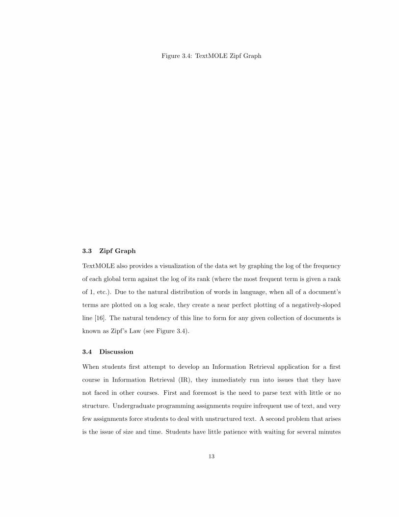
Figure 3.4: TextMOLE Zipf Graph

3.3 Zipf Graph

TextMOLE also provides a visualization of the data set by graphing the log of the frequency

of each global term against the log of its rank (where the most frequent term is given a rank

of 1, etc.). Due to the natural distribution of words in language, when all of a document’s

terms are plotted on a log scale, they create a near perfect plotting of a negatively-sloped

line [16]. The natural tendency of this line to form for any given collection of documents is

known as Zipf’s Law (see Figure 3.4).

3.4 Discussion

When students first attempt to develop an Information Retrieval application for a first

course in Information Retrieval (IR), they immediately run into issues that they have

not faced in other courses. First and foremost is the need to parse text with little or no

structure. Undergraduate programming assignments require infrequent use of text, and very

few assignments force students to deal with unstructured text. A second problem that arises

is the issue of size and time. Students have little patience with waiting for several minutes

13

for a program to parse a moderate-sized file. They tend to assume the program is ‘wrong’

and/or reduce the size of the input file to a impractical size. Weeks of a semester can spent

getting students through these issues. If an instructor wishes to move into a survey advanced

topics in IR or text mining, the IR students are asked to implement a basic search and

retrieval system and then the class moves on to other topics. Issues pertaining to weighting

schemes or indexing options are mentioned in passing, and the impact these parameters

have on retrieval performance tends to be overlooked by students. TextMOLE can be used

to develop an interim assignment which encourages robust exploration of these issues in

indexing without requiring a large amount of programming A week is a reasonable deadline

for students to complete and analysis of a dataset using TextMOLE. Some programming

will most likely be required unless the instructor provides sample datasets which are already

in XML format.

Existing textbooks provide code [2] or refer students to existing retrieval systems, such

as the SMART system [1, 11], but these systems do not tightly integrate indexing and

retrieval, and are difficult for students to install and run. Furthermore, multiple indexing

options and weighting schemes are not implemented (although excellent assignments that

involve adding options to these systems can be developed).

Instructors for courses in Machine Learning (ML) or Artificial Intelligence (AI) may

wish to include a segment on Data Mining or Textual Data Mining. It is impractical to

expect students to overcome the programming issues mentioned above when only a week or

two can be dedicated to a topic. The WEKA tool [15] can be used to model data mining

tasks, but does not address text mining. TextMOLE can be used to fill this gap and provide

students with a solid introduction to IR and Text Mining, which can be leveraged if students

will be asked to complete a final project on some advanced topic in ML or AI.

Adaptions and enhancements TextMOLE would make excellent semester or year long

projects for seniors looking for capstone experiences in computer science.

3.5 Future Work on TextMOLE

Thus far only the foundation for indexing collections of documents and running queries has

been developed. There are many advanced features available to be implemented. The next

version will include options for indexing using noun phrases or n-grams instead of words.

14

Right now the only method of data querying available is vector space retrieval, but more

advanced analyses, such as dimensionality reduction techniques, will be added. In addition,

preprocessing support for data formats other than XML will be built into future versions

of the program. Support for other applications in text mining, such as emerging trend

detection, first-story detection and classification could be added.

15

Chapter 4

Pruning Algorithm

In information retrieval systems which use traditional methods, the level of precision is

very low. Much time and effort has been expended to develop methods to push the most

relevant documents to the top of the query results. Many of these methods have met with

high levels of success; however, the overall precision of all documents returned by a query is

typically still very low [1]. The theoretical optimum is to have each query return only the

documents which are truly relevant to it; in practice, even the most advanced systems (such

as the Google search engine) return huge percentages of the collection which are irrelevant

to the query. I have developed a learning algorithm that can be applied to a collection to

reduce the number of irrelevant documents returned. This algorithm performs unsupervised

learning on query results to discover information about the collection. The algorithm then

uses this information on future queries to prune the results.

In the next section I set up the terminology needed to discuss the learning algorithm.

In Section 4.1, I discuss related work and why this line of research is unique. In Section

4.2, I present an overview of the algorithm and my preliminary results. In Section 4.3, I

offer my concluding comments and present my views on why this technique holds promise

for future research. In Section 4.4, I describe the progress made on automatically setting

dynamic thresholds for the pruning algorithm.

16

4.1 Related Work

Most efforts for improving vector space retrieval concentrate on improving the query by

adding terms using some manner of feedback (often implicit and blind) to improve precision

and/or recall [9, 4]. Since the query becomes much more detailed, the results list has the

documents which match more of the terms closer to the top, and an improvement in precision

often occurs. In one study, improvements in precision at rank 20 ranging from 77-92% were

reported in an idyllic, context-rich scenario [9]. However, in many scenarios where context

was not particularly helpful, the algorithms saw little or no improvement (and even hurt the

results). Unlike the algorithm I developed, these methods do not typically keep a record of

query histories, nor do they directly modify the query results list. My algorithm focuses on

pruning the query results list by actually removing documents.

Methods that do keep track of query histories have done so for purposes of developing a

context for future queries [13, 7]. They assume that queries will follow a logical progression

and attempt to use that sequence to enhance the query’s precision with a variety of methods.

These approaches use the query history to narrow in on what a user is looking for rather

than to assemble an overall perception of the collection. The algorithm presented in the

next section is markedly different in that it treats queries as independent samples.

4.2 Algorithm Overview

Traditional vector space retrieval and other retrieval methods make no provisions for sharing

results between queries. Each query is run independently of every other query. Over the

process of running a batch of queries, the discarding of the query-results information brings

about the loss of data that correlates how documents are related to one another. I have

developed an algorithm that captures and stores query results data so that the data may

be applied to future queries in order to further enhance precision.

The algorithm uses learning techniques to determine which documents are closely related

to one another. When two documents both appear at the top of a ranked list of query results,

the odds of them being related to one another is very high. Conversely, if one document

appears at the top of a ranked query list and another document does not appear at all,

then the odds of them being unrelated are also very high. When recording these statistics

over the span of many queries, the algorithm provides information about the relationships

17

between pairs of documents.

The algorithm can apply this information to query results in order to remove documents.

It does this by taking the top n-ranked documents in the query results list and comparing

their learned relevancies to the other documents returned. If a document has low scores,

according to the learned data, it is removed (it is assumed to be not relevant to the query).

The algorithm can be divided into two distinct phases — the portion which learns the

relationship between documents, and the portion which removes documents from new query

results based on these learned results.

4.2.1 Learning Phase The learning phase is the portion of the algorithm that observes

which documents are returned by queries and then extrapolates and records their relation-

ships.

The Learning Matrix Currently, the algorithm stores the data it learns from queries in

a document-by-document matrix. For each pair of documents a and b in the collection,

there are two entries in the matrix: (a, b) and (b, a). These two entries are distinct to the

algorithm: (a, b) represents the learned similarity score of document b to document a; that

is, the score when a appears higher than b in the sorted query results list, or when a appears

in the list and b does not appear at all. The matrix is not symmetric — it is possible to

have a very strong relation from document a to document b but not vice versa (for example,

if the subject of document b is a specialized topic of a more generalized area discussed by

document a).

Two attributes are recorded during the learning process — the positive associations

and the negative associations. These are recorded separately so that certain situations,

such as whether the documents never appear in any queries, or whether they are equally

positive and negative, are not ambiguous. For example: if positive and negative relationships

were recorded under one summation, then a pair of documents that had a total positive

correlation of 40 and a total negative correlation of 40 would have an identical score to a

pair of documents that never had any correlations recorded. Along with the raw ‘learned

similarity score’, each entry in the matrix also stores the number of queries that contributed

to the score. This is necessary to put the raw score in perspective.

18

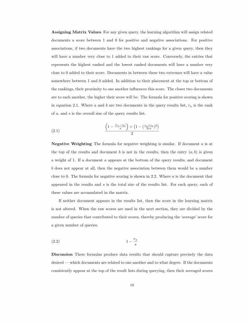
Assigning Matrix Values For any given query, the learning algorithm will assign related

documents a score between 1 and 0 for positive and negative associations. For positive

associations, if two documents have the two highest rankings for a given query, then they

will have a number very close to 1 added to their raw score. Conversely, the entries that

represents the highest ranked and the lowest ranked documents will have a number very

close to 0 added to their score. Documents in between these two extremes will have a value

somewhere between 1 and 0 added. In addition to their placement at the top or bottom of

the rankings, their proximity to one another influences this score. The closer two documents

are to each another, the higher their score will be. The formula for positive scoring is shown

in equation 2.1. Where a and b are two documents in the query results list, ra is the rank

of a, and s is the overall size of the query results list.

(1 − |ra−rb|

s

)+(1 − ( ra+rb

2∗s )2)

2(2.1)

Negative Weighting The formula for negative weighting is similar. If document a is at

the top of the results and document b is not in the results, then the entry (a, b) is given

a weight of 1. If a document a appears at the bottom of the query results, and document

b does not appear at all, then the negative association between them would be a number

close to 0. The formula for negative scoring is shown in 2.2. Where a is the document that

appeared in the results and s is the total size of the results list. For each query, each of

these values are accumulated in the matrix.

If neither document appears in the results list, then the score in the learning matrix

is not altered. When the raw scores are used in the next section, they are divided by the

number of queries that contributed to their scores, thereby producing the ‘average’ score for

a given number of queries.

1 − ra

s(2.2)

Discussion These formulas produce data results that should capture precisely the data

desired — which documents are related to one another and to what degree. If the documents

consistently appear at the top of the result lists during querying, then their averaged scores

19

will be very close to 1. If one document appears and the other never does, then they will have

a negative association between 0 and 1. The value of this negative association is directly

proportional to the height in the rankings of the document that is ranked. In practice, it is

very probable that most entries in the learning matrix will have a combination of positive

and negative scores when training is done.

4.2.2 Document-Removal Phase Once sufficient training has been completed, a

document-removal phase attempts to remove extraneous documents from a query’s results

list. This algorithm is used to post-process the result list produced by traditional vector

space retrieval (described in Section 2.1).

Removal Criteria The algorithm uses several different criteria to determine which

documents should be removed from the results list. In an ideal situation, there would

be a threshold at which all relevant documents had greater positive (or lower negative)

scores, and all non-relevant documents fell below the threshold. Depending on the needs of

the particular system, however, these parameters can be set to remove a larger number of

documents (and potentially remove some relevant documents as well), or ‘play it safe’ and

remove a smaller number of documents and probably not any truly relevant documents.

The algorithm uses the first n documents as a basis for comparison to the rest of the

documents on the list, for it is likely that the majority of those documents are truly relevant

to the query. The algorithm then compares each other document in the results list to each

of those n documents. The ‘threshold’ that these other documents must pass in order to

stay in the results list is twofold: the first test is to see if the average positive score between

the first n documents and the others is greater than a threshold, x, where x is generally 0.7

or greater. The second test is to compare the ratio of positive scores to negative scores —

this number is very dependent on the size of the training set, but with a large amount of

training data, ratios around 20:1 or 15:1 produce good results. This is also dependent on

the general strength of the relationship between documents in a collection. If the collection

pertains to a very specific topic, these ratios may be higher. The second test against the

threshold x is necessary in order to assure that x is not an aberrant score gained by just one

or two positive scores when the correlation between the documents has dozens of negative

scores as well.

20

Training There is one other factor in the algorithm that is heavily dependent on the amount

of training, and that is the percentage of the first n documents for which these thresholds

need to be fulfilled. For example, consider a collection with 1000 documents. After training

on roughly twenty or thirty queries, it is reasonable to expect solid relationships between a

much smaller portion of the n documents to be formed than if you trained on several hundred

queries. With a larger number of trained queries, roughly a third of the n documents should

pass the thresholds for each other document in order to stay in the results list. With a

smaller number of queries, a tenth or a fifth of the first n queries (about 2-3 when using the

first 15 documents) may prove to be sufficient - this will vary depending on the collection.

Discussion It is very important to note that the original precision of queries must be

reasonably high for the first n documents in order for this algorithm to properly weed out

irrelevant documents. If the precision of the original query is too low, then the algorithm

will not function well and will remove relevant documents as readily as irrelevant ones.

Vector space retrieval — without any term weighting on the query or the documents —

provides very minimal benefits when coupled with this approach. This is because normal

vector space retrieval is not accurate without weighting schemes (it essentially just ranks

documents according to whichever has the most number of words from the query). However,

when vector space retrieval uses term-weighting schemes (such as log/entropy or TF/IDF),

then the results are much more promising when coupled with this technique.

4.2.3 Results Current results have had success, as shown in Tables 4.1 and 4.2. Using the

methods described above, I have been able to successfully reduce the number of documents

returned by a query; the number of irrelevant documents removed is typically much greater

than the number of relevant documents removed. The ratio of irrelevant documents removed

to relevant documents removed almost always exceeds the baseline ratio of irrelevant to

relevant in the original results list (if the ratio was not greater, then one might as well pick

documents to remove at random).

The data in Tables 4.1 and 4.2 showcase the algorithm’s effectiveness when applied to

the MED, CACM, and CISI collections. In each case, the algorithm removed on average

89.8% of the documents from each query results list when an aggressive threshold is used.

Precision and recall are calculated using all documents with a similarity score greater than

21

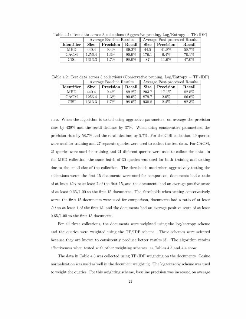
Table 4.1: Test data across 3 collections (Aggressive pruning, Log/Entropy + TF/IDF)Average Baseline Results Average Post-processed Results

Identifier Size Precision Recall Size Precision RecallMED 440.4 9.4% 89.2% 44.5 41.8% 58.7%

CACM 1256.4 1.3% 90.0% 176.1 6.4% 70.1%CISI 1313.3 1.7% 98.0% 87 11.6% 47.0%

Table 4.2: Test data across 3 collections (Conservative pruning, Log/Entropy + TF/IDF)Average Baseline Results Average Post-processed Results

Identifier Size Precision Recall Size Precision RecallMED 440.4 9.4% 89.2% 203.7 17.1% 82.5%

CACM 1256.4 1.3% 90.0% 879.7 2.0% 86.6%CISI 1313.3 1.7% 98.0% 930.8 2.4% 92.3%

zero. When the algorithm is tested using aggressive parameters, on average the precision

rises by 439% and the recall declines by 37%. When using conservative parameters, the

precision rises by 58.7% and the recall declines by 5.7%. For the CISI collection, 49 queries

were used for training and 27 separate queries were used to collect the test data. For CACM,

21 queries were used for training and 21 different queries were used to collect the data. In

the MED collection, the same batch of 30 queries was used for both training and testing

due to the small size of the collection. The thresholds used when aggressively testing the

collections were: the first 15 documents were used for comparison, documents had a ratio

of at least 10:1 to at least 2 of the first 15, and the documents had an average positive score

of at least 0.65/1.00 to the first 15 documents. The thresholds when testing conservatively

were: the first 15 documents were used for comparison, documents had a ratio of at least

4:1 to at least 1 of the first 15, and the documents had an average positive score of at least

0.65/1.00 to the first 15 documents.

For all three collections, the documents were weighted using the log/entropy scheme

and the queries were weighted using the TF/IDF scheme. These schemes were selected

because they are known to consistently produce better results [3]. The algorithm retains

effectiveness when tested with other weighting schemes, as Tables 4.3 and 4.4 show.

The data in Table 4.3 was collected using TF/IDF weighting on the documents. Cosine

normalization was used as well in the document weighting. The log/entropy scheme was used

to weight the queries. For this weighting scheme, baseline precision was increased on average

22

Table 4.3: Test data across 3 collections (Aggressive pruning, TF/IDF/Cosine +Log/Entropy)

Average Baseline Results Average Post-processed ResultsIdentifier Size Precision Recall Size Precision Recall

MED 440.4 9.4% 89.2% 72.5 30.0% 71.3%CACM 1256.4 1.3% 90.0% 210.3 5.8% 74.6%CISI 1313.3 1.7% 98.0% 95.6 12.9% 50.4%

Table 4.4: Test data across 3 collections (Aggressive pruning, No Weighting)Average Baseline Results Average Post-processed Results

Identifier Size Precision Recall Size Precision RecallMED 440.4 9.4% 89.2% 66.5 26.9% 54.4%

CACM 1256.4 1.3% 90.0% 248.5 4.2% 65.1%CISI 1313.3 1.7% 98.0% 241.1 5.7% 57.9%

by 408.1% and the baseline recall was reduced on average by only 28.6% when aggressive

pruning parameters were used. These results are comparable to the results obtained in

Table 4.1.

The data in Table 4.4 was obtained using no weighting parameters. As discussed in

4.2.2, using this pruning algorithm without any term weighting reduces its effectiveness

considerably. However, the pruning algorithm still produces competitive results. Averaged

across the three collections, it increases precision by 214.9% and reduces recall by 35.7%.

The drop in recall in these results occurs when erroneous or misleading information has

been incorporated into the learning matrix. For example, if a document that is actually

relevant to the current query has a negative association — or a lack of a strong positive

association — with all or most (depending on the thresholds) of the documents at the top

of the results list then it would be erroneously removed.

Table 4.5 illustrates the effectiveness of the algorithm by comparing the averaged

precision and recall at ranks 30 and 100 of the (aggressively) pruned query results to the

baseline (unpruned) query results. The log/entropy/cosine normalization scheme was used

to weight the documents and TF/IDF was used to weight the queries for both the pruned

and the baseline results. Many queries returned less than 100 documents. In this case, the

total precision and recall for all these documents is used to calculate its precision and recall

at rank 100. For example, if a query returned 79 documents, then the precision and recall

23

Table 4.5: Aggressive Pruning Performance at Ranks 30 and 100Average Baseline Results Average Post-processed Results

Collection Rank Precision Recall Precision RecallMED 30 45.0% 57.8% 51.7% 61.2%

CACM 30 20.3% 48.1% 26.3% 45.1%CISI 30 20.7% 34.4% 22.4% 35.7%MED 100 18.9% 76.6% 25.2% 71.5%

CACM 100 9.4% 66.4% 14.7% 54.6%CISI 100 10.8% 51.4% 14.6% 44.5%

at rank 79 was used in the calculation of performance at rank 100.

4.3 Discussion

The results so far are promising. The capacity to reduce the size of a query results list from

1000 documents to 200 or 100 documents without losing any relevant documents would be a

revolutionary achievement in information retrieval. When this technique is fully developed,

it will provide a method for creating an extremely high-precision results list with a minimal

loss of relevant data. This would have a positive impact for a wide variety of applications

where high precision is a necessity, such as medical or law databases.

In addition to developing algorithms to minimize the loss of recall within the current

algorithm, another step of the algorithm can be added that attempts to ‘normalize’ the

similarity of the first n documents to each another during removal. Currently the algorithm

assumes that the first n documents are all relevant to the query, even though in practice

this is rarely true. By comparing these initial documents to one another (again using the

learning matrix) documents that do not fit certain criteria can be thrown out — i.e., throw

out documents that are very dissimilar to the rest in the list. This is left to future work.

4.4 Automatic Pruning Parameters

The algorithm can be ’fine-tuned’ to an individual collection in order to greatly increase

performance. This tuning is accomplished by manually setting each of the pruning

parameters to a value that reflects the amount of training and the size and topic density

of the collection. Much of this fine-tuning can be automatically incorporated into the

functionality of the algorithm by scanning the learning matrix prior to document removal

and using statistical facts about the learning matrix to set or tweak the removal parameters.

24

I manually optimized the removal algorithm to the CISI and MED collections, and it resulted

in an increase of precision and recall. These same parameters also provided improvement in

CACM, even though they are not optimized for this collection. When optimization can be

done automatically and dynamically, the effectiveness of the pruning algorithm is increased

dramatically.

Preliminary results into automatically adjusting pruning thresholds are promising but

incomplete. During initial testing an adequate threshold for the average positive score was

set to 0.4∗(1+a), where a is the average positive score in the learning matrix. This equation

ensures that the threshold is always less than one, and will almost certainly be higher than

the average itself (given that the odds of all document pairs being located at the very top

of every query is extremely slim). The constant in the equation is somewhat arbitrary - it

was chosen because it optimized retrieval throughout the three collections tested. Testing

on further collections will be necessary to validate its effectiveness and revise it if necessary.

The threshold for the positive:negative association ratio was set to

0.6 ∗max + 0.4 ∗ avg

2(4.3)

where max and avg are the maximum and average number of queries that had

contributed to a positive relationship in the learning matrix. This equation was also chosen

because it maximized performance across the three collections tested. The balance between

the maximum number of queries and the average represents a valuable characteristic of the

learning matrix: those documents that are closely related will have a much higher ratio

than those which are loosely related or unrelated. Since documents that are very closely

related are desirable, the algorithm leans towards choosing the higher ratios as a threshold.

Table 4.6 describes the results achieved when using these dynamic schemes. The log/entropy

scheme was used to weight the documents and TF/IDF was used to weight the queries.

Experiments to develop an algorithm that accurately chooses how many of the first

n documents in a results list a document must pass the positive:negative ratio threshold

consistently across collections have had inconclusive results. Because of this difficulty, this

threshold was set to 1 for the purposes of collecting the data in Table 4.6. In addition, the

first n documents to use for pruning was fixed at 15.

25

Table 4.6: Automatic Pruning Parameter ResultsAverage Baseline Results Average Post-processed Results

Collection Precision Recall Precision RecallMED 9.4% 89.2% 16.8% 84.6%

CACM 1.3% 90.0% 2.7% 81.8%CISI 1.7% 98.0% 11.0% 50.0%

The experiments described in this section demonstate the potential for automation,

but comprehensive automation of pruning parameters is not complete. Development of a

comprehensive set of threshold equations which produce excellent results across collections

is left to future work.

26

Chapter 5

Conclusion

This work in text-mining presented in this thesis represents a valuable addition to the

collective knowledge of the community. The TextMOLE tool created as part of the thesis is

an extensible, flexible, and robust tool that performs several fundamental text-mining tasks.

TextMOLE has myriad uses for persons of any knowledge level, whether it be as a tool for

learning and instruction, used as an aid for research projects, or extended for a student’s

research or capstone experience. The tool fulfils a need for a simple, clear, and versatile tool

that is specifically designed to assist in text-mining tasks.

The pruning algorithm detailed in this thesis takes a unique approach to query

refinement. It tackles the problem of finding small amounts of relevant data within huge

collections by recording query history information and using this information to prune the

results of future queries. The algorithm utilizes multiple thresholds that test characteristics

of the gathered information to determine which documents are truly relevant to a particular

query. It can be combined with other methods, such as term weighting, to further improve

query results. The results show precision increases from 58.7% to 439% with minimal loss

of recall for the three collections we studied.

27

References

[1] Ricardo Baeza-Yates and Berthier Ribeiro-Neto. Modern Information Retrieval. Addison

Wesley/ACM Press, New York, 1999.

[2] Richard K. Belew. Finding Out About. Cambridge University Press, 2000.

[3] Erica Chisholm and Tamara G. Kolda. New term weighting formulas for the vector space

method in information retrieval. Technical Report ORNL-TM-13756, Oak Ridge National

Laboratory, March 1999.

[4] Cui, Wen, Nie, and Ma. Probabilistic query expansion using query logs. In Proceedings of the

11th international conference on World Wide Web, pages 325–332, Honolulu, Hawaii, USA,

2002.

[5] D. Harman. An experimental study of factors important in document ranking. In Proceedings

of 1986 ACM Conference on Research and Development in Information Retrieval, Pisa, Italy,

1986.

[6] Donna Harman. How effective is suffixing? The American Society for Information Science,

42:7–15, May 1991.

[7] Hayes, Avesani, Baldo, and Cunningham. Re-using implicit knowledge in short-term

information profiles for context-sensitive tasks. In Proceedings of 6th International Conference

on Case-Based Reasoning, Chicago, Illinois, USA, 2005.

[8] Chris Manning and Hinrich Schutze. Foundations of Statistical Natural Language Processing.

MIT Press, Cambridge, MA, 1999.

[9] Mandar Mitra, Amit Singhal, and Chris Buckley. Improving automatic query expansion.

In Proceedings of the 21st annual international ACM SIGIR conference on Research and

development in information retrieval, pages 206–214, Melbourne, Australia, 1998.

[10] Martin F. Porter. An algorithm for suffix stripping. Program, 14(3):130–137, 1980.

[11] Gerard Salton. The SMART Retrieval System–Experiments in Automatic Document Process-

ing. Prentice Hall, Englewood Cliffs, New Jersey, 1971.

[12] Gerard Salton and Michael E. Lesk. The smart automatic document retrieval systems - an

illustration. Commun. ACM, 8(6):391–398, 1965.

[13] Xuehua Shen, Bin Tan, and ChengXiang Zhai. Context-sensitive information retrieval using

implicit feedback. In Proceedings of the 28th annual international ACM SIGIR conference on

Research and development in information retrieval, pages 43–50, Salvador, Brazil, 2005.

[14] C.J. van Rijsbergen. Information Retrieval. Department of Computer Science, University of

Glasgow, 1979.

28

[15] Ian H. Witten and Eibe Frank. Data Mining: Practical Machine Learning Tools and

Techniques, 2nd Edition. Morgan Kaufmann, 2005.

[16] G. Zipf. Human Behaviour and the Principle of Least Effort. Addison Wesley, New York,

1949.

29