The Development of Climate Projections for Use

in Chesapeake Bay Program Assessments

STAC Workshop Report

March 7-8, 2016

Annapolis, MD

STAC Publication 16-006

1

About the Scientific and Technical Advisory Committee

The Scientific and Technical Advisory Committee (STAC) provides scientific and technical

guidance to the Chesapeake Bay Program (CBP) on measures to restore and protect the

Chesapeake Bay. Since its creation in December 1984, STAC has worked to enhance scientific

communication and outreach throughout the Chesapeake Bay Watershed and beyond. STAC

provides scientific and technical advice in various ways, including (1) technical reports and

papers, (2) discussion groups, (3) assistance in organizing merit reviews of CBP programs and

projects, (4) technical workshops, and (5) interaction between STAC members and the CBP.

Through professional and academic contacts and organizational networks of its members, STAC

ensures close cooperation among and between the various research institutions and management

agencies represented in the Watershed. For additional information about STAC, please visit the

STAC website at www.chesapeake.org/stac.

Publication Date: October 2016

Publication Number: 16-006

Suggested Citation:

Johnson, Z., M. Bennett, L. Linker, S. Julius, R. Najjar, M. Mitchell, D. Montali, R. Dixon.

2016. The Development of Climate Projections for Use in Chesapeake Bay Program

Assessments. STAC Publication Number 16-006, Edgewater, MD. 52 pp.

Cover graphic from: Zoë Johnson, NCBO

Mention of trade names or commercial products does not constitute endorsement or

recommendation for use.

The enclosed material represents the professional recommendations and expert opinion of

individuals undertaking a workshop, review, forum, conference, or other activity on a topic or

theme that STAC considered an important issue to the goals of the CBP. The content therefore

reflects the views of the experts convened through the STAC-sponsored or co-sponsored activity.

STAC Administrative Support Provided by:

Chesapeake Research Consortium, Inc.

645 Contees Wharf Road

Edgewater, MD 21037

Telephone: 410-798-1283

Fax: 410-798-0816

http://www.chesapeake.org

2

Workshop Steering Committee:

Mark Bennett, USGS USGS Virginia and West Virginia Water Science Center, 1730 E. Parham Rd, Richmond, VA

23228; mrbennet@usgs.gov; 804-261-2643

Rachel Dixon, CRC/STAC STAC Coordinator, Chesapeake Research Consortium, 645 Contees Wharf Rd., Edgewater, MD,

21037; dixonra@si.edu; 410-798-1283

Zoë Johnson, NOAA NOAA Chesapeake Bay Office, 410 Severn Ave., Suite 207 A, Annapolis, MD, 21401;

zoe.johnson@noaa.gov; 410-267-5656

Susan Julius, EPA/STAC EPA Office of Research and Development, Mailcode 8601P, 1200 Pennsylvania Ave NW,

Washington, DC, 20460; julius.susan@epa.gov; 703-347-8619

Lewis Linker, EPA US EPA Chesapeake Bay Program Office, 410 Severn Ave., Suite 109, Annapolis, MD, 21403;

llinker@chesapeakebay.net; 410-267-5741

Molly Mitchell, VIMS Center for Coastal Resources Management, Virginia Institute of Marine Sciences (VIMS), 1375

Greate Rd., Gloucester Point, VA, 23062; molly@vims.edu; 804-684-7931

Dave Montali, WV DEP West Virginia Department of Environmental Protection, Division of Water and Waste

Management, 601 57th St. SE, Charleston, WV, 25304; david.a.montali@wv.gov; 304-926-0499

Raymond Najjar Jr., PSU/STAC Department of Meteorology and Atmospheric Science, The Pennsylvania State University, 522

Walker Building, University Park, PA 16802; rgn1@psu.edu; 814-863-1586

3

Acknowledgments:

STAC and the Workshop Steering Committee would like to acknowledge Rachel Dixon and

Renee Kelly for their expert guidance and support before, during, and after the workshop. The

Workshop Committee is also especially grateful to the invited speakers and session moderators

for participating fully in the workshop and sharing their expertise, knowledge and experience,

including: Rich Batiuk, EPA/CBPO; Mark Bennett, USGS; Zoe Johnson, NOAA/NCBO; Chris

Weaver, EPA; Ray Najjar, Penn State; Tal Ezer, ODU; Lew Linker, EPA/CBPO; Karen Rice,

USGS; Chris Milly, USGS; Anthony Buda, USDA-ARS; Susan Julius EPA; Gopal Bhatt, PSU;

Barbara Muhling, Princeton/NOAA GFDL; Roger Mann, VIMS; Dick Zimmerman, ODU;

Howard Townsend, NOAA; Molly Mitchell, VIMS ; Kate Johnson, DC; Jennifer DeMooy, DE;

and Phil Morefield, EPA. Success of the workshop was also dependent on the participants

themselves for actively engaging and collaborating to develop recommendations related to the

use and application of climate change projections and scenarios to aid Chesapeake Bay Program

decision-making.

4

Table of Contents Page

Executive Summary 5

Key Findings 7

Recommendations 8

Introduction 9

Section I: Climate Change Projection Needs for Chesapeake Bay Assessments 10

Section II: Approaches for Selecting Climate Scenarios and Projections 11

Section III: Characteristics and Format for Climate Scenarios and Projections 14

Section IV: Selecting Climate Change Scenarios for the 2017 Midpoint Assessment 15

Findings 18

Recommendations 18

Conclusion 19

References 21

Appendix A: Workshop Agenda 23

Appendix B: Workshop Participants 29

Appendix C: Presentation Summaries 31

5

Executive Summary

A workshop entitled Development of Climate Projections for Use in Chesapeake Bay Program

Assessments was organized to help the Chesapeake Bay Program (CBP) assess the applicability

of available climate data, downscaling techniques, projections and scenarios to establish an

approach for climate analysis in CBP models and assessments. The goal of this workshop was to

assist the CBP with the selection process and formulate recommendations for future application

of climate projections in assessments to be undertaken by the Partnership, including modeling

efforts to support the 2017 Midpoint Assessment, as well as other programmatic climate change

impact assessments. The workshop was well attended by climate change scientists as well as

CBP decision-makers and technical managers. A key finding of the workshop was that

substantial scientific understanding currently exists, supporting the need to plan and act on the

ongoing, continuous – but heretofore unrecognized – influence of climate change on Chesapeake

restoration efforts, despite uncertainties.

The workshop centered entirely on technical aspects related to climate science, research, data

and information needs; matters of CBP policy were not addressed. Nevertheless, the workshop

was partly motivated by existing policies, such as the 2010 Total Maximum Daily Load

(TMDL), that call for an assessment of the impacts of a changing climate on Chesapeake Bay

water quality and living resources. The 2014 Chesapeake Bay Agreement also includes 29

individual management strategies, covering a wide range of watershed restoration goals that can

only be sustained over the long term by addressing climate change impacts.

There was consensus at the workshop that the climate change assessment approach should, to the

extent practicable, be made available for application at the regional, state, and local levels.

Although some localities have established climate projections for planning purposes (e.g., sea-

level rise (SLR)), a standardized set of projections and assessment methodology has yet to be

developed for the watershed as a whole. Projections for sea-level, precipitation, air temperature,

water temperature, salinity, and potential evapotranspiration, among others, are needed as inputs

to a variety of hydrological and ecological models, including local TMDL models, to assess

potential future climate impacts on natural and human systems.

The CBP will have to choose among the general circulation models (GCMs), emission scenarios,

downscaling techniques, and historical observation data to establish a framework for climate

analysis in the suite of CBP models. Participants recognized constraints on the CBP, however,

that require them to focus on the year 2025 for short range climate change assessments and

planning in the 2017 Midpoint Assessment. Nevertheless, participants urged the CBP to

examine another period of future scenarios centered on 2050, at the far edge of the planning

horizon, for scoping scenarios. This is because the results of management actions that are in

place by 2025 may not be felt for decades, due in part to the lag times associated with

6

groundwater flow. Meeting the 2017 Midpoint Assessment decision requires the attendant

constraint of selecting a climate change modeling approach that can be applied within the next

six months using the models and other assessment tools at hand.

Workshop consensus was that all aspects of climate and land use change that influence

watershed and Bay should be addressed in the 2017 Midpoint Assessment, as changes in

processes will determine the effectiveness of management actions. Relevant changes include: 1)

air temperature; 2) precipitation; 3) sea-level; 4) wind speed and direction; 5) humidity; and 6)

atmospheric deposition of nitrogen. These changes in the climate system are expected to alter

key variables and processes within the Chesapeake Bay and its watershed, including

evapotranspiration, soil moisture, streamflow, water temperature, salinity, estuarine circulation,

and key water quality variables (e.g., water clarity, chlorophyll, and dissolved oxygen). These

climate changes should be examined in concurrence with land use changes that will interact with

and potentially exacerbate climate change impacts. To the extent practicable, the effect of all of

these changes on key living resources such as wetlands, submerged aquatic vegetation (SAV),

and oysters should also be assessed.

Workshop participants recommended the use of historical (~100 years) trends to project

precipitation to 2025 for purposes of the Midpoint Assessment, as opposed to utilizing an

ensemble of future projections from GCMs. Shorter term climate change projections using

GCMs have large uncertainties because climate models are structured to look further out and at

much larger scales. Participants in the workshop shared varied perspectives on the topic of

uncertainty and climate projections. One recurring perspective was that uncertainty in some

climate change projections is high, particularly for precipitation volumes and intensities across

the Chesapeake watershed. There are inherent limitations in projecting precipitation, particularly

its intensity, from existing regional statistical and dynamical downscaling of GCMs because they

don't take adequate account of mesoscale processes that are important in water dynamics.

Furthermore, extrapolating short term trends in precipitation is particularly risky. There are

strong cyclic variations associated with climate models that impact shorter term precipitation

trends and make longer term projections difficult.

Participants recommended that for long-term assessments (2050 and beyond) the CBP use an

ensemble or multiple global climate model approach, selecting model outputs that bound the

range of key climate variables (e.g., temperature, precipitation) for the Chesapeake Bay region.

The use of multiple scenarios covering a range of projected emissions (representative

concentration pathways (RCP) 4.5 and 8.5, as currently being utilized for Fourth National

Climate Assessment) was recommended along with the inclusion of the 2 °C emissions reduction

pathway (RCP 2.6). Lastly, participants advised the CBP to use an existing system to access

GCM downscaled scenario data (such as ‘LASSO’ described in more detail in Section II) in lieu

7

of conducting a tailored statistical climate downscaling process for the Chesapeake Bay

watershed.

Multiple tools are already available to assess the impacts of climate change on the Chesapeake

Bay watershed and its living resources. The Chesapeake Bay Watershed Model (CBWM), the

Chesapeake Bay Water Quality and Sediment Transport Model (WQSTM), and living resource

models such as models of SAV, tidal wetlands, and oysters, will be used to examine the impact

of climate change on water quality and estuarine ecosystems during the 2017 Midpoint

Assessment. Over time however, other assessment tools could be added to examine the impact

of climate change as it relates to additional 2014 Chesapeake Agreement Goals and Outcomes.

Key Scientific Findings

1. There is sufficient scientific understanding to provide insights into the decisions faced by

the CBP over the short and long term to anticipate and manage for unavoidable climate

change.

2. There is strong confidence in continued warming trends, recognizing that there is inter-

annual variability.

3. There is less confidence that the watershed will experience an increase in the intensity of

precipitation; there may be more variability, with a significant trend annually, but not in all

seasons.

4. There is wider agreement on the seasonal precipitation changes (wetter winters and springs,

potentially drier summers) than overall annual precipitation changes, although it is likely

that both will occur.

5. Projected trends in discharge are likely to differ from those in precipitation. Timing of

rainfall, antecedence, and evapotranspiration are contributing factors to the differences in

observed discharge and precipitation trends for the Chesapeake Bay.

6. There are inherent limitations in projecting precipitation, particularly its intensity, from

existing regional statistical and dynamical downscaling of GCMs because they don't take

adequate account of mesoscale processes that are important in water dynamics.

7. Extrapolating short term trends in precipitation is particularly risky. There are strong cyclic

variations associated with climate models that impact shorter term precipitation trends and

make their use in longer term projections difficult.

8. Climate models are structured to look further out and at much larger scales than current

management goals (i.e., 2025 Chesapeake Bay Agreement goals and outcomes). By 2025,

the end of the policy horizon, anthropogenic drivers within GCMs are just beginning to act

in ways that clearly differentiate the anthropogenic impacts from the other cyclical drivers

of climate.

9. For the purposes of the Midpoint Assessment modeling approach, projections for 2025

should be considered in terms of a 30-year projection from 1995 (mid-point of 1991 to 2000

8

Chesapeake Bay TMDL simulation period) through 2025, and the analysis of climate trends

should be based on long term historical trends. Climate models and analyses of short-term

(<50 years) data are not suitable for short-range projections because they include decadal-

scale weather cycles which lead to large uncertainties in short-term trends.

Recommendations

The workshop culminated with the following specific recommendations related to the selection,

use, and application of climate projections and forecasts for the 2017 Midpoint Assessment.

1. The Partnership should seek agreement on the use of consistent climate scenarios for regional

projections of Chesapeake Bay condition and the benefits of an integrated source of climate

change projection simulation data that all seven jurisdictions could draw from.

2. For the 2017 Midpoint Assessment, use historical (~100 years) trends to project precipitation

to 2025 as opposed to utilizing an ensemble of future projections from GCMs. Shorter term

climate change projections using GCMs have large uncertainties because climate models are

structured to look further out and at much larger scales.

3. The Partnership should carefully consider the representation of evapotranspiration in

Watershed Model calibration and scenarios because the calculation method for

evapotranspiration has a strong influence on the strength and direction of future water

balance change.

4. Looking forward, the 2050 timeframe is more appropriate for selecting and incorporating a

suite of global climate scenarios and simulations to provide long-term projections for the

management community, and an ongoing adaptive process to incorporate climate change into

decision-making as implementation moves forward.

5. Beyond the 2017 Midpoint Assessment, it is recommended that the CBP use 2050

projections for best management practice (BMP) design, efficiencies, effectiveness,

selection, and performance – given that many of the BMPs implemented now could be in use

beyond 2050.

6. For any 2050 assessment, use an ensemble or multiple global climate model approach,

selecting model outputs that bound the range of key climate variables (e.g., temperature,

precipitation) for the Chesapeake Bay region. Use multiple scenarios covering a range of

projected emissions (RCP 4.5 and 8.5 are a reasonable range to select and are currently being

utilized for Fourth National Climate Assessment). Include the 2 °C emissions reduction

pathway (RCP 2.6) as well as more "business as usual" assumptions.

7. Select an existing system to access GCM downscaled scenario data (such as ‘LASSO’

described in more detail in Section II) in lieu of conducting a tailored statistical climate

downscaling process for the Chesapeake Bay watershed.

9

Introduction

The 2014 Chesapeake Bay Agreement includes 29 individual strategies to be developed and

implemented by six Goal Implementation Teams (GITs). Most, if not all, of these strategies will

include a suite of actions necessary to address climate change impacts. In addition, the 2010

Total Maximum Daily Load (TMDL) documentation and the 2009 Executive Order call for an

assessment of the impacts of a changing climate on Chesapeake Bay water quality and living

resources that will be addressed during the upcoming 2017 Midpoint Assessment.

The Chesapeake Bay Watershed Model (CBWM), the Chesapeake Bay Water Quality and

Sediment Transport Model (WQSTM), and living resource models, such as models of

underwater grasses, tidal wetlands, and oysters, will be used to examine the impact of climate

change on water quality and estuarine ecosystems. Other assessment tools will be utilized to

examine the impact of climate change on other goals and outcomes. Although some localities

have established climate projections for planning purposes (e.g., sea-level rise), a standardized

set of projections has yet to be developed for the Watershed. Such projections for sea-level rise,

precipitation, air temperature, and potential evapotranspiration, among others, are needed as

inputs to a variety of hydrological and ecological models to assess potential future climate

impacts on natural and human systems.

The 2014 Intergovernmental Panel on Climate Change (IPCC) report relied on the Coupled

Model Intercomparison Project, featuring approximately 30 global general circulation models

(GCMs), each with multiple emission scenarios. Additionally, there are multiple downscaling

techniques that are available to move from these global-scale models to an appropriate scale for

the Chesapeake Bay and its watershed. Extrapolation of decades of historical observations of

temperatures, precipitation intensity, precipitation volume, sea-level rise, and estuarine salt

intrusion have also been used to assess future scenarios as a result of climate change (IPCC-

TGICA 2007).

The Chesapeake Bay Program (CBP) will have to choose among the GCMs, scenarios,

downscaling techniques, and historical observation data to establish an approach for climate

analysis in the CBP models. The goal of this workshop was to assist the CBP with the selection

process and formulate recommendations for future application of climate projections in

assessments to be undertaken by the Partnership, including modeling efforts to support the 2017

Midpoint Assessment, as well as other programmatic climate change impact assessments.

On March 7-8, 2016, the Scientific and Technical Advisory Committee (STAC) of the CBP

conducted a workshop entitled “The Development of Climate Projections for Use in Chesapeake

Bay Program Assessments.” Over the course of the workshop, approximately 50 attendees

participated and actively engaged in discussion sessions. The goal of the workshop was to

10

conduct a review of GCMs, scenarios, downscaling techniques, and historical observation data

for the purposes of helping the CBP assess the applicability of available climate data and

establish a framework for climate analysis in the CBP models. The workshop agenda (Appendix

A) was centered on answering the following questions:

1. What climate change variables are of most concern to the CBP partners in the

consideration of the 2017 Midpoint Assessment decisions and for longer term climate

change management decisions?

2. What are the approaches that can be taken to select climate change scenarios for CBP

assessments?

3. What characteristics of those climate variables need to be specified, such as the temporal

and spatial resolution, in order to provide the most utility at the regional, state, and local

levels?

4. What climate change scenarios meet CBP decision-making needs for the 2017 Midpoint

Assessment as well as for longer term climate change management decisions and

programmatic assessments?

The body of the following report addresses the four above questions in separate dedicated

sections. Within the text, links to workshop presentations and other references are provided; all

workshop presentations and other associated materials can be found at

http://www.chesapeake.org/stac/workshop.php?activity_id=258.

Section I: Climate Change Data and Projection Needs for Chesapeake Bay Assessments

The 2010 Chesapeake Bay TMDL is the largest, most complex TMDL in the country, covering a

166,000 km2 area across seven jurisdictions. The Bay TMDL allocates loadings of nitrogen,

phosphorus, and sediment to sources and areas of the watershed contributing those pollutants to

remove impairments for aquatic life in the Bay’s tidal tributaries and embayments. A successful

TMDL relies on good water quality standards. In the Chesapeake, the water quality standards

were based on what living resources require to persist and thrive. The Chesapeake TMDL has

water quality standards of dissolved oxygen (DO) in four separate habitats (deep channel, deep

water, open water, and migratory fish regions), a chlorophyll standard (both narrative and

numeric) and a water clarity/submerged aquatic vegetation (SAV) standard to ensure healthy

shallow water regions of the Bay.

Throughout the workshop, the following three climate variables external to the Bay-watershed

system emerged as being of most concern to long-term management of the Chesapeake Bay and

its watershed:

11

(1) Air temperature (Najjar, workshop presentation): This variable has a profound effect

on the functioning of the Bay and its watershed through impacts on evapotranspiration

(which influences soil moisture and streamflow), water temperature, and indirectly on

streamflow, biogeochemical rates (such as nitrification and denitrification), habitat

suitability (e.g., for seagrasses and fish), and oxygen solubility, among others.

(2) Precipitation (Najjar, workshop presentation): The delivery of freshwater, nutrients, and

sediment to the Bay is mainly driven by the amount and intensity of precipitation in the

watershed. Thus, Bay circulation and water quality strongly respond to changes in

watershed precipitation.

(3) Sea-level (Ezer, workshop presentation): Tidal wetlands, which are a major feature of

the Bay’s living resources, are strongly influenced by sea-level. Bay circulation and

salinity are also affected by sea-level.

Other climate variables may be important to consider as well, such as wind speed and direction,

humidity, and downwelling solar and longwave radiation, which variably influence

evapotranspiration, water temperature, and estuarine circulation. The atmospheric CO2

concentration also has importance beyond its influence on the climate, as an increase in CO2

leads to ocean acidification.

Addressing the challenge of climate change impacts on Chesapeake water quality standards will

be difficult; the Clean Water Act requires that water quality standards must be met regardless of

potential impacts. In 2017, the CBP partnership will decide if, when, and how to incorporate

climate change considerations into the Phase III Watershed Implementation Plans (WIPs).

Among the Bay Program partners, discussions have begun on how future changes in

precipitation volume and intensity could change stormwater and other management practices

(DeMooy, workshop presentation; Johnson workshop presentation), or how sea-level rise

impacts communities and tidal wetlands (Ezer, workshop presentation).

The CBP partners are developing the tools to quantify the effects of climate change on watershed

flows and loads, storm intensity, increased estuarine temperatures, sea-level rise, and ecosystem

influences including loss of tidal wetland attenuation with sea-level rise, as well as other

ecosystem influences on key living resources.

Section II: Approaches for Selecting Climate Scenarios and Projections

From a high-level perspective of framing the need for and selection of climate change scenarios,

two paradigms exist: the first and most dominant assumes a need to predict using physically-

based computer models to support planning efforts; the second emphasizes the need to

understand regional and sectoral climate-related vulnerabilities and how to manage in light of

12

large uncertainties associated with climate change and its possible impacts. Both approaches are

used as a basis to select climate change scenarios, but the first requires accurate predictions in

order to support adaptation planning while the second supports adaptation planning that focuses

on robust solutions to cover a range of potential climate change outcomes (Weaver, workshop

presentation).

Climate scenarios are developed using a GCM driven by emissions scenarios. The most recent

emissions scenarios developed by the IPCC employ representative concentration pathways

(RCPs). RCPs are an expression of future radiative forcing, or the change in net downwelling

infrared radiation at the Earth’s surface by the year 2100 caused by changes in atmospheric

constituents, such as carbon dioxide. The four principal scenarios – RCP 2.6, RCP 4.5, RCP 6.0

and RCP 8.5 – range from a low emissions scenario in which greenhouse gas concentrations

reach a maximum in 2040 and decline to levels slightly above current levels by 2100 (RCP 2.6),

to a high emissions scenario in which greenhouse gas concentrations continuously increase,

reaching values roughly a factor of three higher than current values (RCP 8.5). Choosing climate

change scenarios requires selecting the emissions scenarios, the specific GCMs that run those

emission scenarios, and, in some cases particular realizations of those GCMs (a realization being

a specific run of the GCM with a very slightly altered initial state) (Morefield, workshop

presentation).

Currently, there are more than 35 GCMs. Climate scenario data from these GCMs can be used

directly or can be downscaled using several different methods. Downscaling generally refers to

the manipulation of a coarser resolution dataset to create data with finer resolution. The two

general approaches for downscaling are statistical and dynamical. There is no consensus on a

single best downscaling approach.

In statistical downscaling, empirical relationships between large-scale and local-scale variables

like temperature and precipitation are developed based on historical observations via a variety of

methods. The technique is based on the principle that both the large-scale climate state and local

physiographic features act together to determine local climate. The major advantage of statistical

downscaling is the relative computational efficiency compared to dynamical downscaling. They

are also flexible and effective at removing errors in historical simulated values. This provides a

good match between the average (multi-decadal) statistics of observed and statistically

downscaled climate at the spatial scale, and over the historical period of the observational data

used to train the statistical model. A shortcoming of this approach is the assumption that the

statistical relationships between coarse- and fine-resolution variables created using historical data

will also hold in the future under a changing climate. This assumption may be valid for lesser

amounts of change, but could lead to errors, particularly in precipitation extremes with larger

amounts of climate change. A number of databases provide statistically downscaled projections

for a range of higher and lower future scenarios for the contiguous United States. Examples

13

include the Multivariate Adaptive Constructed Analogs (MACA) (Abatzoglou and Brown 2012)

and monthly Bias-Corrected and Statistically Downscaled (BCSD) projections (Reclamation

2013).

Dynamical downscaling uses outputs from GCMs to establish boundary conditions for finer

resolution simulations using Regional Climate Models (RCMs) within a limited area of the globe

(e.g., the Northwest or Southeast U.S.). Several advantages of dynamical downscaling are

internal consistency among different variables based on physical principles, the ability to

investigate the specific physical processes and system dynamics that lead to the simulated

changes, and higher resolution data (typically on the order of 10-50 km horizontal grid mesh).

RCMs are subject to the same types of uncertainty as global models, such as not fully resolving

physical processes that occur at even smaller scales. They also have additional uncertainty

related to how often their boundary conditions are updated and where they are defined. These

uncertainties can have a large effect on the precipitation simulated by the models at the local to

regional scale. RCM simulations for the U.S. are available from several sources, the most

common and comprehensive being the North American Regional Climate Change Assessment

Program (NARCCAP).

There are a number of readily available sources climate change planning scenarios (e.g., U.S.

Climate Resilience Toolkit, USGS Geo Data Portal). There are fewer tools available, however,

that can be used to guide users through the process of selecting scenarios for specific

assessments. One tool presented at the workshop is “Locating and Selecting Scenarios Online”

(LASSO). LASSO pulls from all publicly available climate model outputs to provide data

visualizations that illuminate the characteristics of the different scenarios. These visualizations

support scenario selections tailored to the decision context and sensitivities of the system or

species being assessed (Morefield, workshop presentation).

Participants at the workshop advocated the use of a multiple model/multiple scenario approach to

represent different emission scenarios (RCPs). The recommended RCPs include RCP 2.6, which

assumes that global annual greenhouse gas emissions peak by about 2020 consistent with the

United Nations Framework Convention on Climate Change, 2015 Paris Agreement. RCP 2.6

could constrain the increase of global mean surface temperature to less than 2 oC and this could

be used to define a minimum baseline for CBP adaptation. However, there are also good reasons

to assume that world-wide emissions consistent with RCP 2.6 will be difficult to achieve and

therefore RCP 4.5, which assumes a moderate growth in emissions peaking by about 2040,

should also be considered in addition to RCP 8.5, which assumes a high growth in CO2

equivalent emissions that continue to rise throughout the 21st century.

The application of new approaches to ensemble modeling was also encouraged including the

LASSO tool (Morefield, workshop presentation) and other approaches in order to keep the

14

number of climate change scenarios at a feasible operational level (Buda, workshop presentation;

Muhling, workshop presentation).

Section III: Characteristics and Format for Climate Scenarios and Projections

For each modeling effort to be undertaken by the CBP in order to determine future climate

change impacts on the Bay, its watershed, and the associated living resources, there is a need to:

define specific data needs (e.g., historical observations/trends, future projections, climate

variables); determine data requirements (e.g., range of scenarios vs. sole variable); establish

spatial extent (e.g., geographic relevance); and select temporal scale (e.g., seasonal, inter-annual,

decadal and beyond).

Workshop presenters provided an overview of the data needs and format for temporal and spatial

drivers to complete both watershed scale physical and biological and ecological climate change

assessments. Presentations made on key Chesapeake living resources assessments of SAV

(Zimmerman), oysters (Mann), tidal wetlands (Mitchell), and ecosystems (Townsend),

highlighted some important considerations regarding the application of climate data to

Chesapeake Bay assessments, while other speakers provided feedback on decision points and the

process for selecting specific climate change indicators for more generalized local, state, and

regional assessments (Muhling, DeMooy, Johnson, Ezer, Buda). Take-away points from the

presentations and discussion that followed are:

● Geographic relevance: When looking at the Bay as a whole, there is a danger of

glossing over regional differences (e.g., Eastern shore of Virginia vs. Norfolk) because

changes in some resources (such as tidal marshes) may be location-specific on a

relatively small scale (Mitchell).

● Climate variability: It is critical to examine the role of climate variability and not just

long-term change. Synoptic climate patterns (such as the Bermuda High) and variations

in climate modes that operate on interannual (El Niño/Southern Oscillation (ENSO)) and

decadal (Pacific Decadal Oscillation (PDO)) scales influence the climate of the

Chesapeake region (Townsend).

● Non-climate related drivers: Impacts from climate change are likely to interact

synergistically with those from changes in land use and other human factors. For

example, it is not just increasing atmospheric CO2 that is driving pH change, but also

changes in estuarine photosynthesis and respiration resulting from enhanced nutrient

loads from the watershed. It is difficult to tease out which complex climate drivers vs.

non-climate drivers dominate the observed impacts and to predict the impact of these

drivers into the future (Mann). While air temperature and precipitation are key drivers to

15

understand, both local estuarine and watershed dynamics are also important for predicting

estuarine conditions (Muhling).

● Secondary climate drivers: For SAV, turbidity may have a bigger impact in the Bay

than nutrient loading, so there is a need for more data and information on storm incidence

(Zimmerman). Other climate drivers to consider include wind speed and direction.

Given their significance, we should examine how to include these components beyond

the midpoint assessment timeframe of 2025.

● Varying timescales, non-linearity and feedback loops: Biologic response occurs over

varying timescales and species and organisms evolve together over time; changes in one

will effect changes in another (Mann).

● Sea-level rise parameters: For sea-level rise, assessments can make use of both past

(historic) measurements and future estimates. In terms of geographic scale, projections

on global sea-level rise are too large for practical local and regional planning and there is

a need to consider the linear rate of change as well as the acceleration. Projections based

on statistics of past sea-level data may be useful in the short term but do not take into

account potential long-term changes (Ezer).

● Seasonal, hourly and daily data: Several speakers (Buda, DeMooy, Johnson, Bhatt)

spoke of the need for climate variables at hourly and/or daily resolution to serve as useful

input for modeling climate change impacts.

● Importance of locally relevant climate indicators: Both DeMooy and Johnson spoke

on the importance of selecting climate change indicators that matter to decision-makers.

Delaware and the District of Columbia (DC) have undertaken projects to generate

downscaled climate projections that are locally relevant. For both jurisdictions, climate

scenarios for RCP 4.5 and 8.5 were derived and a suite of climate indicators were

referenced to individual long-term weather stations. Delaware selected temperature and

precipitation indicators and DC selected the same but also added in extreme events.

Despite the general availability of climate change data and information and a fairly concerted

effort by researchers within the watershed to gain a better understanding of climate trends and

impacts, many questions remain to be answered: how will the water balance change with climate

change; will streamflow increase or decrease?; how will the frequency of floods and low flows

change?; how will climate change affect extremes?

Section IV: Selecting Climate Change Scenarios for the 2017 Midpoint Assessment and

Beyond

The Chesapeake Bay Program has identified the need to develop a 2025 climate change scenario

to support the 2017 Midpoint Assessment. A constant ten-year average hydrology was used to

establish the 2010 Chesapeake TMDL. The hydrologic period for TMDL modeling purposes is

16

the period that represents the long-term average hydrologic conditions for the waterbody. This is

important so that the Bay models can simulate local long-term average conditions for each area

of the Bay watershed and tidal waters to ensure that no single area is modeled with a particularly

high or low loading, an unrepresentative mix of point and nonpoint sources, or extremely high or

low river flow. The selection of the representative hydrologic averaging period that ensured a

balance between high and low river flows across the Bay watershed was the 1991-2000

hydrology (USEPA 2010).

The use of a constant ten-year average hydrology ensured stationarity and prevented assessment

of climate change because of the fixed and unchanging temperatures and hydrology. The

application of a 2025 year scenario allows for the adjustment of the ten-year hydrology to reflect

climate change effects. In essence, the 2025 scenario is actually a 30 year projection of climate

change from a base of 1995, the mid-point of the 1991-2000 hydrology. The use of a 2025

future period is due to the third and last phase of the WIPs, which are designed to complete the

implementation of management practices in order to achieve tidal water quality standards, cover

the period of 2018 to 2025. Altogether, the 2025 scenario will provide the CBP partnership the

tool to decide when, and how to incorporate climate change considerations into the Phase III

WIPs.

Workshop presentations by Linker (workshop presentation) and Bhatt (workshop presentation),

described aspects of the 2025 scenario. Bhatt described an extrapolation of observed

precipitation data from 1984 to 2014, which developed spatially and temporally detailed

(seasonal) data for the Chesapeake Bay and watershed and suggested that shortcomings of

relying solely on the recent three decades of precipitation could be overcome by constraining the

volume of extrapolated precipitation to that of the long term precipitation record. That record,

described by Rice (workshop presentation) in her presentation of long-term historical

precipitation and flows from the 1920s to present, would provide for long-term trends that would

be isolated by decadal climate oscillations such as the North Atlantic Oscillation (NAO) and

other similar phenomena. Rice also stated that trends in long-term precipitation do not often

match long-term trends in discharge due to a variety of factors including timing of rainfall,

antecedent moisture conditions, and evapotranspiration, among others. Other workshop

presentations, including Najjar (workshop presentation) and Ezer (workshop presentation)

discussed aspects of historical trends for the watershed and sea-level rise, respectively.

Workshop participants recommended the use of recent regional sea-level rise (RSLR) projections

such as described by Ezer (workshop presentation), which incorporates glacial rebound,

groundwater withdrawals, Chesapeake bolide impact crater, and Gulf Stream influence. A recent

effort in Maryland to project RSLR based on regional expert consensus can be found here:

http://www.umces.edu/sites/default/files/pdfs/SeaLevelRiseProjections.pdf, which found a mean

estimate for 2050 relative SLR (over 2000) of 0.4 m (0.2-0.7 m). This is consistent with the 0.5

17

m used in the dissolved oxygen scenario modeling, which represents a baseline change from

1995 (mid-point of the 1991-2000 average hydrology used in the Chesapeake TMDL).

However, as in all climate projections, this will depend on the emissions pathway.

Overall, workshop participants supported the approach of a 2025 scenario, but recognized that

the detailed extrapolation of trends based on 1984-2014 trends were insufficient. Furthermore,

there is a need for trends to be augmented and constrained by additional long-term information

from other sources such as the observed precipitation and discharge trend record described by

Rice (workshop presentation). Relying solely on the extrapolation of recent trends in

precipitation fails to account for strong cyclic variations associated with ENSO, the PDO, the

North Atlantic Oscillation (NAO), the Atlantic Multidecadal Oscillation, and other climate

modes.

For long-term climate change management decisions and programmatic assessments, the

selection of a 2050 scenario was recommended. Muhling (workshop presentation), Weaver

(workshop presentation), and other presenters indicated that a 2050 scenario would be within an

envelope where strong anthropogenic influence on climate would have traction allowing

ensembles of climate models to be used. At the same time, the 2050 scenario would be useful as

an engineering design point for capital projects with a design life of several decades, such as

large stormwater facilities and other water resource structures. The 2050 scenario would also

accommodate the time needed for some management actions to be fully effective, due to, for

example, the lag times associated with groundwater flow. Participants recommended using an

ensemble approach for 2050 utilizing downscaled climate variables from a number of GCMs that

would be considered representative of the region.

Although the use of downscaled information from GCM’s was recommended for 2050 scenario

assessments, it was not recommended for 2025 scenario development. A more simplistic

approach of using historical extrapolations was recommended for 2025 scenario development.

This recommendation reflects the ability of climate models to capture anthropogenic impacts on

the climate over larger spatial and temporal scales, which makes them more applicable for 2050

and beyond scenarios. By 2025, the anthropogenic drivers have not yet started to act in a way

that differentiates the anthropogenic impact from the other cyclical drivers of climate.

There is strong confidence in continued warming trends, recognizing that there is year to year

variability, but less confidence in projections of precipitation volume and intensity. The

approach used for representing evapotranspiration in the projections is also a large part of the

uncertainty (Milly, workshop presentation). The interaction of changing precipitation amounts,

timing of rainfall, and evapotranspiration result in streamflow projections that are characterized

by uncertainty with large consequences for nutrient and sediment loading.

18

Findings

A summarized list of findings based on presentations and discussions that occurred among

workshop participants is as follows:

1. There is sufficient scientific understanding to provide insights into the future on what the

CBP should be doing over the short and long term to anticipate and manage for unavoidable

climate change.

2. There is strong confidence in continued warming trends, recognizing that there is

interannual variability.

3. There is less confidence that the watershed will experience an increase in the intensity of

precipitation; there may be more variability, with a significant trend annually, but not in all

seasons.

4. There is wider agreement on the seasonal precipitation changes (wetter winters and springs,

potentially drier summers) than overall annual precipitation changes, although it is likely

that both will occur.

5. Projected trends in discharge are likely to differ from those in precipitation. Timing of

rainfall, antecedence, and evapotranspiration are contributing factors to the differences in

observed discharge and precipitation trends for the Chesapeake Bay.

6. There are inherent limitations in projecting precipitation, particularly its intensity, from

existing regional statistical and dynamical downscaling of GCMs because they don't take

adequate account of mesoscale processes that are important in water dynamics.

7. Extrapolating short term trends in precipitation is particularly risky. There are strong cyclic

variations associated with climate models that impact shorter term precipitation trends and

make their use in long-term projections difficult.

8. Climate models are structured to look further out and at much larger scales than current

management goals (i.e., 2025 restoration goals). By 2025, the end of the policy horizon,

anthropogenic drivers within GCMs are just beginning to act in ways that clearly

differentiate the anthropogenic impacts from the other cyclical drivers of climate.

9. For the purposes of the Midpoint Assessment modeling approach, projections for 2025

should be considered in terms of a 30-year projection from 1995 (mid-point of 1991 to 2000

Chesapeake Bay TMDL simulation period) through 2025 and the analysis of climate trends

should be based on long term historical trends. Climate models and analyses of shorter-term

(<50 years) data are not suitable for short-range projections because they include decadal-

scale weather cycles which lead to large uncertainties in short-term trends.

Recommendations The workshop culminated with the following specific recommendations related to the selection,

use and application of climate projections and forecasts for the 2017 Midpoint Assessment:

19

1. The Partnership should seek agreement on the use of consistent climate scenarios for regional

projections of Chesapeake Bay condition and the benefits of an integrated source of climate

change projection simulation data that all seven jurisdictions could draw from.

2. For the 2017 Midpoint Assessment, use historical (~100 years) trends to project precipitation

to 2025 as opposed to utilizing an ensemble of future projections from GCMs. Shorter term

climate change projections using GCMs have large uncertainties because climate models are

structured to look further out and at much larger scales.

3. The Program should carefully consider the representation of evapotranspiration in watershed

model calibration and scenarios because the calculation method for evapotranspiration has a

strong influence on the strength and direction of future water balance change.

4. Looking forward, the 2050 timeframe is more appropriate for selecting and incorporating a

suite of global climate scenarios and simulations to provide long-term projections for the

management community, and an ongoing adaptive process to incorporate climate change into

decision-making as implementation moves forward.

5. Beyond the 2017 Midpoint Assessment, it is recommended that the CBP use 2050

projections for best management practice (BMP) design, efficiencies, effectiveness,

selection, and performance – given that many of the BMPs implemented now could be in the

ground beyond 2050.

6. For any 2050 assessment, use an ensemble or multiple global climate model approach,

selecting model outputs that bound the range of key climate variables (e.g., temperature,

precipitation) for the Chesapeake Bay region. Use multiple scenarios covering a range of

projected emissions (RCP 4.5 and 8.5 are a reasonable range to select and are currently being

utilized for Fourth National Climate Assessment). Include the 2 °C emissions reduction

pathway (RCP 2.6) as well as more "business as usual" assumptions.

7. Select an existing system to access GCM downscaled scenario data (such as ‘LASSO’

described in more detail in Section II) in lieu of conducting a tailored statistical climate

downscaling process for the Chesapeake Bay watershed.

Conclusion

Workshop consensus was that all aspects of climate change that influence Chesapeake Bay

watershed should be addressed in the 2017 Midpoint Assessment, including changes in: 1) air

temperature, 2) precipitation, 3) sea-level, 4) wind speed and direction, 5) humidity, and 6)

atmospheric deposition of nitrogen. These changes in the climate system are expected to alter

key variables and processes within the Chesapeake Bay and its watershed, including

evapotranspiration, soil moisture, streamflow, water temperature, salinity, estuarine circulation,

and key water quality variables (e.g., water clarity, chlorophyll, and dissolved oxygen). These

climate factors should be looked at in coincidence with land use changes that will interact with

20

and potentially exacerbate climate change impacts. To the extent practicable, the effect of all of

these changes on key living resources such as wetlands, SAV, oysters, and other living resources

should be assessed.

There was consensus at the workshop that the climate change assessment should, to the extent

practicable, be available for application at the regional, state, and local levels. Although some

localities have established climate projections for planning purposes (e.g., sea-level rise), a

standardized set of projections has yet to be developed for the watershed. Projections for sea-

level, precipitation, air temperature, water temperature, salinity, and potential evapotranspiration,

among others, are needed as inputs to a variety of hydrological and ecological models, including

local TMDL models, to assess potential future climate impacts on natural and human systems.

Drawing from the findings and recommendations presented at the workshop and summarized in

this document, the CBP, with input from CBP’s Modeling and Climate Resiliency Workgroups,

should develop the proposed climate change assessment framework for the 2017 Midpoint

Assessment. To initiate this process, workshop participants identified three near term key

actions:

1. Convene a group of climate researchers to reach agreement on several key points,

including but not limited to:

a. Determination of a baseline

b. Key variables to consider (temperature, precipitation, sea-level rise)

c. Suite of GCMs to apply for Midpoint Assessment Needs; and living resources

(SAV, Oysters, and Fish) assessment needs

d. Downscaling techniques and Potential Evapotranspiration (PET) models to apply

e. Range of scenarios to run

f. Process to evaluate above modeling outputs

2. Convene a group of sea-level rise researchers and resource experts to reach agreement on

sea-level rise estimates to apply; how to best approach simulating effect of sea-level rise

on living resources (SAV, Oysters, Fish) and wetlands, and the range of sea-level rise

scenarios to run.

3. The Climate Resiliency Workgroup should provide guiding principles to the jurisdictions

to consider while developing their Phase III WIPs.

21

References

Abatzoglou J.T. and T.J. Brown. 2012. A comparison of statistical downscaling methods suited

for wildfire applications. International Journal of Climatology 32(5): 772-780.

Bureau of Reclamation. 2013. Downscaled CMIP3 and CMIP5 Climate and Hydrology

Projections: Release of Downscaled CMIP5 Climate Projections, Comparison with preceding

Information, and Summary of User Needs’. U.S. Department of the Interior, Bureau of

Reclamation, Technical Services Center, Denver, Colorado. 47 pp.

Collins, M., R. Knutti, J. Arblaster, J.-L. Dufresne, T. Fichefet, P. Friedlingstein, X. Gao, W.J.

Gutowski, T. Johns, G. Krinner, M. Shongwe, C. Tebaldi, A.J. Weaver and M. Wehner, 2013:

Long-term Climate Change: Projections, Commitments and Irreversibility. In: Climate Change

2013: The Physical Science Basis. Contribution of Working Group I to the Fifth Assessment

Report of the Intergovernmental Panel on Climate Change [Stocker, T.F., D. Qin, G.-K. Plattner,

M. Tignor, S.K. Allen, J. Boschung, A. Nauels, Y. Xia, V. Bex and P.M. Midgley (eds.)].

Cambridge University Press, Cambridge, United Kingdom and New York, NY, USA.

IPCC AR5 WG1. 2013. Stocker, T.F., et al., eds., Climate Change 2013: The Physical Science

Basis. Working Group 1 (WG1) Contribution to the Intergovernmental Panel on Climate Change

(IPCC) 5th Assessment Report (AR5), Cambridge University Press.

IPCC-TGICA. 2007. General Guidelines on the Use of Scenario Data for Climate Impacts and

Adaptation Assessment. Version 2. Prepared by T.R. Carter on behalf of the Intergovernmental

Panel on Climate Change, Task Group on Data and Scenario support for Impact and Climate

Assessment. 66 pp.

Moss, R., et. al. 2008. Towards New Scenarios for Analysis of Emissions, Climate Change,

Impacts, and Response Strategies. Geneva: Intergovernmental Panel on Climate Change. 25 pp.

USAID. 2014. A Review of Downscaling Methods for Climate Projections. United States

Agency for International Development by Tetra Tech ARD, through a Task Order under the

Prosperity, Livelihoods, and Conserving Ecosystems (PLACE) Indefinite Quantity Contract

Core Task Order (USAID Contract No. AID-EPP-I-00-06-00008, Order Number AID-OAA-TO-

11-00064). USAID, Washington, DC. 42 pp.

U.S. Federal Government, 2014: U.S. Climate Resilience Toolkit.

[Online] http://toolkit.climate.gov.

22

United Nations Framework Convention on Climate Change (UNFCCC). 2015. Conference of

the Parties: Adoption of the Paris Agreement. FCCC/CP/2015/L.9. Paris, France.

U.S. EPA. 2010. Chesapeake Bay Total Maximum Daily Load for Nitrogen, Phosphorus and

Sediment. U.S. Environmental Protection Agency Chesapeake Bay Program Office, Annapolis,

Maryland.

23

Appendix A: Workshop Agenda

The Development of Climate Projections for Use in Chesapeake

Bay Program Assessments

Scientific and Technical Advisory Committee (STAC) Workshop

March 7-8 2016

Westin Annapolis, 100 Westgate Circle, Annapolis MD 21401

Workshop Goals

The 2014 Chesapeake Bay Agreement includes 29 individual strategies to be developed and

implemented by six Goal Implementation Teams (GITs). Most, if not all, of these strategies will

include a suite of actions necessary to address climate change impacts. In addition, the 2010

TMDL documentation and the 2009 Executive Order call for an assessment of the impacts of a

changing climate on the Chesapeake Bay water quality and living resources that will be

addressed during the upcoming 2017 Midpoint Assessment.

The Chesapeake Bay Watershed Model, the Chesapeake Bay Water Quality and Sediment

Transport Model (WQSTM), and living resource models, such as models of underwater grasses,

tidal wetlands, and oysters, will be used to examine the impact of climate change on water

quality and estuarine ecosystems. Other assessment tools will be utilized to examine the impact

of climate change on other goals and outcomes. Although some localities have established

climate projections for planning purposes (e.g., sea-level rise), a standardized set of projections

has yet to be developed for the watershed. Such projections for sea-level rise, precipitation, air

temperature, storm intensity, and potential evapotranspiration, among others, are needed as

inputs to a variety of hydrological and ecological models to assess potential future climate

impacts on natural and human systems.

The 2014 Intergovernmental Panel on Climate Change (IPCC) report relied on a Coupled Model

Intercomparison Project featuring approximately 30 global general circulation models (GCMs),

each with multiple emission scenarios. Additionally, there are multiple downscaling techniques

that are available to move from these global-scale models to an appropriate scale for the

Chesapeake Bay and its watershed. Extrapolation of decades of historical observations of

temperatures, precipitation intensity, precipitation volume, sea level rise, and estuarine salt

intrusion have also been successfully used for future scenarios of climate change.

The Chesapeake Bay Program (CBP) will have to choose among the GCMs, scenarios,

downscaling techniques, and historical observation data to establish a framework for climate

analysis in the CBP models. The goal of workshop is to assist the CBP with the selection process

by addressing the following questions:

24

1. What climate change variables are of most concern to the CBP partners in the

consideration of the 2017 Midpoint Assessment decisions and for longer term climate

change management decisions?

2. What are the approaches that can be taken to select climate change scenarios for CBP

assessments?

3. What characteristics of those climate variables need to be specified, e.g., temporal,

spatial, and other relevant characteristics? In what format are scenarios needed to

provide the most utility at the regional, state, and local levels?

4. What climate change scenarios meet CBP decision-making needs for the 2017

Midpoint Assessment as well as for longer term climate change management

decisions and programmatic assessments?

Day 1: Monday, March 7

8:30 Registration, light breakfast (provided)

9:00 Welcome Address – Rich Batiuk, U.S. EPA Chesapeake Bay Program

9:10 Introduction and Purpose of Workshop – Mark Bennett, USGS

Session I: Introduction and Background

9:25 Climate Change Impacts of Most Concern for Chesapeake Bay Agreement Goal and

Outcome Attainment – Zoe Johnson, NOAA/CBPO

9:45 Use of Climate Change Scenarios for Supporting Decision Making – Chris Weaver,

U.S. EPA

10:15 Climate Change in the US with an Emphasis on the Northeast: Past, Present, and

Future – Ray Najjar, Penn State A presentation on how climate has changed in the Northeast region, how it is expected to

change in the future and how extrapolation of past trends can be used for short range 10-

15 year projections of climate change.

10:45 Sea-level Rise for the Chesapeake Bay Area: Causes, Trends, and Future

Projections – Tal Ezer, Center for Coastal and Physical Oceanography, ODU The various aspects that contribute to local sea level rise in the region and the impact on

flooding will be reviewed. These include global sea level rise, land subsidence, and

response to oceanic and atmospheric dynamic, such as potential climatic changes in the

Gulf Stream. The difficulty of estimating future sea level rise will be discussed.

25

11:15 DISCUSSION (Moderator: Lew Linker, EPA/CBPO) What are the approaches that can be taken to develop climate change scenarios for

Chesapeake Bay Program decision-making? What are the important climate drivers and

time periods for assessment of climate change impacts for the 2017 Midpoint Assessment

as well as for longer term climate change management decisions?

12:00 LUNCH (provided)

Session II: Case-Study Examples of Climate Trend Assessments,

Data, and Scenario Needs for CBP Climate Assessments of the

Watershed and Estuary

Overview: This session will provide short, concise presentations on climate change information

needs for past and ongoing CBP assessments in the watershed and tidal estuary. Each presenter

will provide an overview of data needs and format for temporal and spatial climate drivers to

complete the assessment.

1:00 Historical Flow Trends – Karen Rice, USGS Trends in precipitation and flow in different Chesapeake watersheds will be examined.

1:20 Evapotranspiration – Chris Milly, USGS The presentation will examine the challenges in the simulation of climate-model-implied

growth in potential evapotranspiration.

1:40 Assessing the Hydrologic and Water Quality Impacts of Climate Change in Small

Agricultural Basins of the Upper Chesapeake Bay Watershed – Anthony Buda,

USDA-ARS This presentation will examine projected trends in statistically downscaled climate data

for a representative agricultural basin of the Upper Chesapeake Bay watershed and

outline a proposed approach for assessing the impacts of these trends on watershed

hydrology and water quality using the Soil and Water Assessment Tool.

2:00 Patuxent River Case Study (Urban Storm Water) – Susan Julius, U.S. EPA A study of the application of a scenario selection process in an urban watershed and the

findings of that study will be discussed.

2:20 Approaches to the Simulation of Climate Change with the CBP Watershed and

Estuarine Model – Gopal Bhatt, PSU; Ping Wang, VIMS; and Guido Yactayo,

UMCES Initial scenarios generated by the Watershed Model based on an extrapolation of

observed precipitation based trends and projected to the years 2025 and 2050 will be

26

presented and estimates of the influence sea-level rise and temperature increases have on

Bay water quality will be discussed.

2:40 2017 Midpoint Assessment Management Needs – Lewis Linker, U.S. EPA

Chesapeake Bay Program and Carl Cerco, USACE-ERDC Initial work done to support an assessment of how climate change in 2025 and 2050

could influence achieving Chesapeake water quality standards will be presented,

including simulations of the influence of changes in watershed loads, sea level rise,

estuarine temperature increases, and tidal marsh loss.

3:00 Break

3:15 DISCUSSION (Moderator: Ray Najjar, PSU) What specific climate data are needed for ongoing or planned assessments? In what

format are climate data needed: temporal scale (e.g., 2025, 2050, 2100); spatial scale

(e.g., field scale, watershed scale, regional scale); and what variables (e.g., min, max

daily temp, extreme precipitation events vs. mean annual changes).

4:30 Adjourn Day One

Day 2: Tuesday, March 8

8:00 Registration, light breakfast (provided)

8:30 Welcome, Summary of Day 1, and Comments from Workshop Participants

Session III: Case-Study Examples of Climate Trend Assessments, Data, and

Scenario Needs for CBP Climate Assessments of Ecosystems

Overview: This session will provide short, concise presentations on climate change information

needs for past and ongoing CBP assessments in key ecosystems. Each presenter will provide an

overview of data needs and format for temporal and spatial climate drivers to complete the

assessment.

8:45 Downscaling Climate Models for Ecological Forecasting In Northeast U.S. Estuaries

– Barbara Muhling, Princeton/NOAA GFDL Statistical downscaling is commonly used to convert global climate model outputs to a

regional scale. The results of recent downscaling experiments for the Chesapeake Bay

and Susquehanna watershed will be discussed, along with consideration of variability

among downscaling methods.

9:15 Impacts of Climate Change on Chesapeake Oysters – Roger Mann and Ryan

Carnegie, VIMS Oysters provide ecosystem services in the Chesapeake Bay as benthic pelagic couplers,

as structural complexity (reefs) in the benthos, and as central components in the bay

27

alkalinity budget. All are subject to change in response to projected climate change: (1)

What is the impact of climate driven changes in temperature and/or salinity on oysters,

oyster diseases and the oyster-disease interaction; (2) what is the impact of changing

water chemistry on oysters in both the larval and adult life history stages; (3) what is the

impact of (1) and (2) combined on oyster population dynamics and the role of oysters as

an alkalinity bank; and (4) can we proactively manage any of it?

9:45 Zostera & SAV Response to Projected Temperature and CO2 Concentrations –

Victoria Hill & Dick Zimmerman, ODU

10:05 Climate Change and Ecological Forecasting in the Chesapeake Bay – Howard

Townsend, NOAA

10:25 Loss of Coastal Marshes to Sea-level Rise – Molly Mitchell, VIMS Molly Mitchell, of the VIMS Center for Coastal Resources Management will describe a

survey and analysis of wetland loss due to sea level rise in the Chesapeake as well as data

and modeling needs for assessing climate change impacts on tidal wetlands.

10:55 Break

Session IV: Climate Scenarios, Projections, and Realizations - What Do We

Have and What Do We Need?

Overview: This session will focus on approaches to selecting climate change scenarios for the

Chesapeake Bay Program that fit the needs of local, state, and regional partners and stakeholders.

One key focus of this session is to identify approaches for streamlining scenario selection while

maintaining analytic consistency and rigor across the Program.

11:05 State Perspectives on Climate Change Scenario Selection – Kate Johnson, DC and

Jennifer DeMooy, DE Both Delaware and the District have used statistical downscaling for climate change

impact assessments. Why they chose the particular downscaling approach used and how

the downscaled projection will be applied in their respective states will be described.

11:35 A Climate Scenario Selection Tool – Phil Morefield, U.S. EPA

12:05 DISCUSSION (Moderator: Susan Julius, EPA) What climate change scenarios meet Chesapeake Bay Program decision-making needs

for the 2017 Midpoint Assessment as well as for longer term climate change management

decisions? In what format are realizations needed that will provide the most utility at the

regional, state, and local levels? Is there a need for consistency among climate change

scenarios across the watershed and state and local jurisdictions?

12:30 LUNCH (provided)

28

1:30 WRAP UP DISCUSSION (Moderator: Rich Batiuk, U.S. EPA Chesapeake Bay

Program) There are many physical, biological, and ecological changes that will take place in a

Chesapeake Bay influenced by climate change. In order to better evaluate future

behavior of the entire system of watershed, airshed, estuary, and ecosystem under a

variety of adaptive climate change management strategies, what are the most important

climate data and information needs? This includes considerations of what, when, where,

and how to sample the watershed, estuary, and ecosystem as well as how to best

synthesize research, observations, and model analysis in order to improve understanding

of how the system is changing and adaptive management approaches. Also, what

laboratory and field studies should be undertaken to better understand past trends and

project future impacts.

In addition to the short and long-term CBP science priorities, we need to consider what

steps are needed to make the best use of the current state of our understanding to evaluate

management decisions that must be made in the next year as a part of the 2017 Midpoint

Assessment. In particular, what are the most important improvements that should be

made to the suite of models (watershed and Bay) in order to better predict how climate

change will modulate the transport and fate of nutrients and sediment to tidal waters and

how that will affect the achievement of the TMDL goals in the Bay?

2:30 Adjourn

29

Appendix B: Workshop Participants

Name Affiliation Contact

Batiuk, Rich EPA-CBPO Batiuk.Richard@epa.gov

Bennett, Mark USGS-CBPO mrbennet@usgs.gov

Bhatt, Gopal PSU-CBPO gbhatt@chesapeakebay.net

Blakenship, Karl Bay Journal bayjournal@earthlink.net

Boesch, Don UMCES boesch@umces.edu

Buda, Anthony PSU Anthony.Buda@ars.usda.gov

Coles, Victoria UMCES vcoles@umces.edu

Currey, Lee MDE lee.currey@maryland.gov

Dalmasy, Dinorah MDE dinorah.dalmasy@maryland.gov

DeMooy, Jennifer DNREC Jennifer.DeMooy@state.de.us

Dixon, Keith (remote) NOAA/OAR/GFDL Keith.Dixon@noaa.gov

Dixon, Rachel CRC/STAC Staff dixonra@si.edu

Ezer, Tal ODU TEzer@odu.edu

Freidrichs, Marjy VIMS marjy@vims.edu

Hill, Victoria ODU VHill@odu.edu

Hinson, Kyle CRC khinson@chesapeakebay.net

Idhe, Tom NOAA-NCBO tom.ihde@noaa.gov

Johnson, Kate DOEE katherine.johnson@dc.gov

Johnson, Tom EPA johnson.thomas@epa.gov

Johnson, Zoe NOAA-CBPO zoe.johnson@noaa.gov

Julius, Susan EPA-ORD/STAC julius.susan@epa.gov

Kelly, Renee CRC/STAC Staff kellyr@si.edu

Linker, Lew EPA-CBPO LLinker@chesapeakebay.net

Mann, Roger VIMS rmann@vims.edu

Merritt, Melissa CRC mmerritt@chesapeakebay.net

Michael, Bruce MD DNR bruce.michael@maryland.gov

Milly, Chris USGS cmilly@usgs.gov

Mitchell, Molly VIMS molly@vims.edu

Montali, Dave WV DEP david.a.montali@wv.gov

Morefield, Phil EPA morefield.philip@epa.gov

Muhling, Barbara NOAA GFDL/Princeton barbara.muhling@noaa.gov

Najjar, Raymond PSU/STAC najjar@metero.psu.edu

Rice, Karen USGS kcrice@usgs.gov

Sabo, Robert EPA sabo.robert@epa.gov

Shenk, Gary USGS-CBPO GShenk@chesapeakebay.net

Sincock, Jennifer (remote) EPA Sincock.Jennifer@epa.gov

Spano, Tanya MWCOG tspano@mwcog.org

30

Stoner, Anne (remote) Texas Tech anne.stoner@ttu.edu

Tian, Richard UMCES rtian@chesapeakebay.net

Townsend, Howard NOAA-NCBO howard.townsend@noaa.gov

Volk, Jennifer UDEL jennvolk@udel.edu

Wang, Ping VIMS PWang@chesapeakebay.net

Weaver, Chris EPA weaver.chris@epa.gov

Wilusz, Dano JHU dwilusz1@jhu.edu

Yactayo, Guido UMCES-CBPO gyactayo@chesapeakebay.net

Zimmerman, Robert ODU RZimmerm@odu.edu

31

Appendix C: Presentation Summaries

Session 1: Introduction and Background

Climate Change Impacts of Most Concern for Chesapeake Bay Agreement Goal and Outcome

Attainment – Zoe Johnson, NOAA/CBPO

Recognizing the need to gain a better understanding of the likely impacts as well as potential

management solutions for the watershed, a new goal was added to the 2014 Chesapeake Bay

Watershed Agreement, committing the Chesapeake Bay Program partnership to take action to

“increase the resiliency of the Chesapeake Bay watershed, including its living resources,

habitats, public infrastructure and communities, to withstand adverse impacts from changing

environmental and climate conditions.” This new goal builds on the 2010 TMDL documentation

and the 2009 Presidential Executive Order 13508, which also call for an assessment of the

impacts of a changing climate on the Chesapeake Bay water quality and living resources.

Chesapeake Bay Program (CBP) partners are currently working on several fronts to formulate

plans, conduct modeling and other assessments, and align existing monitoring programs to gain a

better understanding of the trends and likely impacts of a changing climate. Modeling and

monitoring efforts will be used to ultimately inform the development of specific adaptation

strategies and targeted restoration and protection activities, as well as evaluate progress towards

reducing the impact of climate change over time.

In December 2015, the CBP Scientific and Technical Advisory Committee (STAC) undertook a

planning exercise to help inform the program’s prioritization of climate change impacts of most

concern with respect to the Chesapeake Bay Agreement. During the facilitated exercise, STAC

members were asked to: 1) explore and discuss aspects of climate change, which may impact the

achievement of individual goals and outcomes (e g., restore x acres of wetlands by year xxxx); 2)

assign a qualitative (low, medium, high) factor of risk in terms of the influence of future climate

impact on “goal/outcome attainment”; and 3) to identify research needs to fill critical

information gaps. Results of the first phase of this planning exercise are presented in Figure 1.

Figure 1. Goal Attainment: Qualitative Factor of Risk

Goal Outcome Qualitative Factor

of Risk

Primary Climate

Drivers

Water Quality 2025 WIP Outcome Medium SLR, T, P, EE

WQ Attainment High (over long‐

term)

SLR, T, P, EE

Healthy Watersheds Healthy Waters Varied response T, P, EE

32

Vital Habitats Black Duck High SLR

Brook Trout High T, P

Wetlands Medium (non‐

tidal)/High (tidal)

SLR, P

Stream Health High T, P

SAV HIgh SLR, T, EE

Forest Buffer Medium SLR, P, EE

Urban Tree Canopy Medium T, P

Land Conservation Protected Lands Low ‐ Medium SLR

Public Access Low ‐ Medium SLR

Sustainable Fisheries Blue Crab Medium T

Oyster Restoration Medium T, OA

Fish Habitat High SLR, T, P, EE

Forage Fish High SLR, T, P

Building from the STAC analysis, the CBP will be using a suite of model applications, including

the Chesapeake Bay Watershed Model, the Chesapeake Bay Water Quality and Sediment

Transport Model (WQSTM), and a number of living resource models to examine the impact of

climate change on the Chesapeake Bay watershed and its ecosystems. Other assessment tools

will be utilized to examine the impact of climate change on other goals and outcomes. Specific

climate change projections or scenarios to guide programmatic assessments have yet to be

developed. Projections for sea-level rise, precipitation, air temperature, storm intensity, and

potential evapotranspiration, among others, are needed as inputs to a variety of hydrological and

ecological models to assess potential future climate impacts on natural and human systems.

At the very basic level, for each modeling effort to be undertaken, there is a need to define

specific data needs (e.g., historical observations/trends, future projections, climate variables);

determine data requirements (e.g., range of scenarios vs. sole variable); establish spatial extent

(e.g., geographic relevance); and select temporal scale (e.g., seasonal, inter-annual, decadal and

beyond).

The Use of Climate Change Scenarios for Supporting Decision-Making – Chris Weaver, U.S.

EPA

Climate change presents numerous unique challenges to effective, science-based decision

support. In particular, while the methods, practices, and tools of health and ecological risk

33

assessment have provided the foundation for EPA’s ability to leverage the best-available science

to meet its mission to protect human health and the environment, the character of the climate

change problem is proving difficult to accommodate within traditional risk assessment

frameworks.

One major challenge is the presence of deep uncertainty about future climate changes, and its

associated impacts. This uncertainty results from lack of predictability of future climate change

due to natural year-to-year and decade-to-decade variability in the climate system; potentially

large and poorly understood feedbacks (e.g., carbon cycle feedbacks); the uncertain trajectory of

key anthropogenic drivers, especially greenhouse gas emissions; and uncertainty about how

human systems will respond and adapt. These limits on climate system predictability are felt

most strongly at precisely the space and time scales most relevant for environmental

management, such as the regional and local scales of watersheds and communities, or for short-

term extremes such as heavy rainfall events. What this means in practical terms is that, not only

is the past no longer a reliable guide to the future, but it will often be difficult to describe

expected future climate change and impacts with well-characterized probability distributions

around ‘most likely’ future conditions.

Rather than dependence on highly

imperfect predictions of future climate

conditions and impacts of greatest

relevance for watershed management,

use of scenarios within ‘bottom-up’ or

‘robust’ decision frameworks

(Paradigm 2) can help overcome these

uncertainty-based challenges, as well as

help address intrinsic barriers

(cognitive, behavioral, institutional) to

good decision making.

The choice of initial set of scenarios will need to reflect the shift in decision framework

- Choose initial scenarios that most clearly bound the decision-relevant climate changes, in

the face of multiple uncertainties, rather than produce a contingent probability

distribution around a ‘most likely’ future value. This is a natural consequence of

focusing on societal risk, where a disproportionate fraction of total risk will often be

associated with low-probability outcomes (‘tail risks’).

- Choose initial scenarios that most clearly distinguish between futures in which your

policies succeed and those in which they fail. These will most often be composed of

variables with (a) highest impact on management endpoints and (b) highest levels of

uncertainty.

34

Climate Change in the Northeast US: Past, Present, and Future – Raymond Najjar, The

Pennsylvania State University

The climate of the Northeast United States (US), including the Mid-Atlantic Region that the

Chesapeake Bay and its watershed lie in, has undergone change over the past century or so.

Observational trends were summarized by Kunkel et al. (2013a,b) and are reported here.

Although interannual variability is substantial, annual mean temperature and precipitation in the

Northeast US have undergone significant long term increases of about 2 °F and 10%,

respectively. Extreme precipitation has increased as well. Like the rise in global mean

temperature, there is high confidence that the primary cause in the temperature increase of the

Northeast US is an increase in greenhouse gases (Kunkel et al. 2013a), a conclusion drawn in

part from simulations of regional climate with and without increases in greenhouse gas

concentrations. On the other hand, it appears that natural climate variability has dominated the

observed precipitation increase, as climate models do not consistently simulate a precipitation

increase when greenhouse gas increases are included in them. Furthermore, there are significant

statistical linkages between Mid-Atlantic precipitation and climate modes, particularly El

Niño/Southern Oscillation and the Pacific Decadal Oscillation, on decadal time scales (Schulte et

al. 2016).

Climate model projections in the Northeast US indicate substantial changes (Kunkel et al. 2013a,

b). The average warming among 15 climate models by 2035 is nearly 3 °F and is essentially

independent of emissions scenario due to the long lifetime of CO2 in the atmosphere and the

large thermal inertia of the climate system (mainly the ocean). By 2055 the average warming is

sensitive to the emissions scenario, with 2085 projections of nearly 5 °F and 8 °F warming under

the B1 and A2 scenarios, respectively (which are bracketed by the RCP 2.6 and 8.5 scenarios

discussed in the body of this report). There is high confidence that the historical warming trend

will continue into the future as not a single climate model projects cooling. About 80% of global

climate models project increased precipitation in the Northeast US into the 21st century; the

average increase by 2085 is about 5%, with a modest sensitivity to the emissions scenario. There

is a greater increase and a greater consensus for precipitation in the winter and spring (~15%

average increase among the models by mid-21st century), and a suggestion that summer

precipitation may decline slightly. Finally, climate models consistently project an increase in the

intensity of precipitation in the Northeast US as greenhouse concentrations continue to increase.

By the mid-21st century, the mean increase in precipitation intensity (defined as the number of

days per year with precipitation above 1 inch) is typically between 10 and 20% throughout the

Chesapeake Bay watershed.

In summary, the Chesapeake Bay watershed has become warmer and wetter, and precipitation

has become more intense. These trends can be expected to continue throughout the 21st century,

35

but natural variability is likely to create cycles in precipitation that will periodically enhance and

weaken its long-term increase.

References:

Kunkel, K.E., L.E. Stevens, S.E. Stevens, L. Sun, E. Janssen, D. Wuebbles, J. Rennells, A.

DeGaetano, and J.G. Dobson. 2013a. Regional Climate Trends and Scenarios for the U.S.

National Climate Assessment, Part 1. Climate of the Northeast U.S., NOAA Technical

Report NESDIS 142-1. U.S. Department of Commerce, Washington, D.C., 79 pp.

Kunkel, K.E., L.E. Stevens, S.E. Stevens, L. Sun, E. Janssen, D. Wuebbles, C.E. Konrad II, C.M.

Furhrman, B.D. Keim, M.C. Kruk, and A. Billot. 2013b. Regional Climate Trends and

Scenarios for the U.S. National Climate Assessment, Part 2. Climate of the Southeast U.S.,

NOAA Technical Report NESDIS 142-2. U.S. Department of Commerce, Washington,

D.C., 94 pp.

Schulte, J., R.G. Najjar, and M. Li. 2016. The influence of climate modes on streamflow in the

Mid-Atlantic Region of the United States. Journal of Hydrology: Regional Studies 5, 80-99.

Sea-level Rise for the Chesapeake Bay Area: Causes, Trends, and Future Projections – Tal

Ezer, Center for Coastal and Physical Oceanography, ODU

The sea level rise (SLR) around the Chesapeake Bay (CB) is one of the highest of all U.S. coasts and the

rates are accelerating. Local SLR rates over the past 10-30 years are ~4-6 mm/year, which are higher than

the global mean SLR rates of ~1.7 mm/year over the past century or even higher than the ~3.2 mm/year

over the past 20 years as seen from satellite altimeter data. There are also variations within the CB, with

rates that are higher in the south part of the bay and slightly lower in the north and along the eastern shore

of Virginia. This SLR results in acceleration in the frequency and periods of flooding (see Figure below).

36

Relative SLR in CB is primarily the result of three processes: 1) global SLR due to warming ocean

temperatures and melting land ice, 2) local land subsidence, and 3) changes in ocean and atmospheric

dynamics. The CB’s coasts are experiencing subsidence due to recent human activities such as

groundwater extraction and long-term Glacial Isostatic Adjustment (GIA) since the end of the ice age.

Climatic changes and weakening in the Gulf Stream appear to result in increased coastal sea-level and

flooding. Remote influence from climate patterns such as El-Nino and the North Atlantic Oscillation

(NAO) can also impact the region, but they are difficult to predict.

Projections of future SLR in the region need to take all these factors into account by combining data and

models. For relatively short-term projections of 10-20 years or so, statistical projections based on

analysis of linear and non-linear past trends may be useful, but for longer projections, say 50-100 years,

climate models that take into account future greenhouse emission scenarios and increasing melting of ice

sheets are needed.

ODU’s Climate Change and Sea Level Rise Initiative (http://www.odu.edu//research/initiatives/ccslri)

and the Center for SLR (http://www.centerforsealevelrise.org/) address those issues; recent research

papers from these activities are listed below (PDFs available at

http://www.ccpo.odu.edu/~tezer/Pub.html).

References:

Ezer, T. and W.B. Corlett. 2012. Is sea-level rise accelerating in the Chesapeake Bay? A demonstration

of a novel new approach for analyzing sea level data, Geophysical Research Letters 39: L19605,

doi:10.1029/2012GL053435.

Ezer, T. L.P. Atkinson, W.B. Corlett and J.L. Blanco. 2013. Gulf Stream's induced sea-level rise and

variability along the U.S. mid-Atlantic coast, Journal of Geophysical Research 118(2): 685-697,

doi:10.1002/jgrc.20091.

Ezer, T. 2013. Sea level rise, spatially uneven and temporally unsteady: why the U. S. east coast, the

global tide gauge record and the global altimeter data show different trends, Geophysical Research

Letters 40(20): 5439-5444 doi:10.1002/2013GL057952.

Atkinson, L.P., T. Ezer and E. Smith. 2013. Sea-level rise and flooding risk in Virginia, Sea Grant Law

and Policy Journal 5(2): 3-14.

Ezer, T. and L.P. Atkinson. 2014. Accelerated flooding along the U. S. East Coast: On the impact of sea

level rise, tides, storms, the Gulf Stream and the North Atlantic Oscillations. Earth's Future 2(8): 362-

382 doi:10.1002/2014EF000252.

37

Ezer, T. 2015. Detecting changes in the transport of the Gulf Stream and the Atlantic overturning

circulation from coastal sea-level data: The extreme decline in 2009-2010 and estimated variations for

1935-2012. Global and Planetary Change 129: 23-36. doi:10.1016/j.gloplacha.2015.03.002.

Ezer, T. 2016. Can the Gulf Stream induce coherent short-term fluctuations in sea level along the U.S.

East Coast?: A modeling study. Ocean Dynamics 66(2): 207-220. doi:10.1007/s10236-016-0928-0.

Session II: Case Study Examples of Climate Trend Assessments, Data, and Scenario Needs

for CBP Climate Assessments of the Watershed and Estuary

Historical Flow Trends – Karen Rice, USGS

Analysis of Long-Term Hydrologic Records in the Chesapeake Bay Watershed

Karen C. Rice1,2 and Douglas L. Moyer1 1U.S. Geological Survey, Virginia Water Science Center 2University of Virginia

Hydrologic data were analyzed to determine the relations between long-term precipitation and

long-term discharge trends in the Chesapeake Bay (CB) watershed. Previous research on runoff

from 1930 through 2010 indicates that some flow metrics, for example, the mean one-day

maximum runoff, show differences in their trends between northern and southern watersheds

(Rice and Hirsch 2012). The north-south dividing line is approximately the Pennsylvania—

Maryland border (Rice and Hirsch 2012). The amount, frequency, and intensity of precipitation

have increased in the eastern United States (U.S.), however, the observed increases have been

greater in the northeast than the southeast (Karl and Knight, 1998; U.S. Climate Assessment,

2014). The 165,759-square kilometer (km2) CB watershed spans the north-to-south gradient in

precipitation increases.

Daily mean discharge data were obtained for 27 U.S. Geological Survey (USGS) gaging stations

in and near the CB watershed for calendar years 1927 through 2014. The watersheds have

diverse land use and span areas from 303 to 62,419 km2. PRISM

(http://www.prism.oregonstate.edu/historical/) precipitation data (Daly et al. 2008) were

downloaded and spatially and temporally averaged to obtain mean monthly data specific to each

of the 27 watersheds from 1927 through 2014. The objectives of the talk presented at the CB

Scientific and Technical Advisory Committee workshop were to: (1) determine if and how the

changes in precipitation are being manifested as changes in discharge; (2) identify any spatial

differences in the precipitation—discharge relations; and (3) compare these evaluations of the

historical record (1927-2014) to the period specific to the CB Program’s Watershed Model

(1985-2014).

38

Annual distributions of daily mean discharge and monthly total precipitation for each watershed

were analyzed; values of precipitation and discharge corresponding to each decile (0th, 10th,

20th,…100th) were assembled for each year; linear regressions were fitted for the whole period

for each decile, and slopes and p-values (at the α ≤ 0.05 level) were recorded. The spatial

patterns in significant increasing (≤ 0.05) precipitation and discharge trends in the deciles

differed between the northern and southern watersheds. Among the northern watersheds, the

number of sites with significant increasing precipitation was highest for the 60th, 70th, and 80th

deciles, whereas the number of sites with significant increasing discharge was highest for the 0th

through 60th deciles. Among the southern watersheds, significant increasing trends in

precipitation occurred only in the 50th, 60th, and 70th deciles. In contrast, significant increasing

trends in discharge occurred in the 0th through 20th deciles and in the 50th through 90th deciles. In

general, the linkage between precipitation and discharge was less in the southern watersheds as

compared with those in the north. Also in the south, trends in precipitation had lower slopes;

there were fewer significant precipitation and discharge trends, and the significance of the trends

decreased; and, among the deciles, there were fewer significant trends (Rice and others, 2016).

The disconnect between precipitation and discharge trends might be explained by the basic

hydrology of watersheds, whereby lag times, travel times, land use, snow pack and timing of

snowmelt, antecedent conditions, and evapotranspiration all influence the nature of the

manifestation of the precipitation on discharge. There were far more significant increasing

trends for the historical record (1927-2014) of discharge than for the period specific to the

Watershed Model (1985-2014) across all deciles. The discrepancy in the number of significant

increasing trends between the two periods can be attributed to the quantitative power of a linear

trend test, which is highly sensitive to the number of observations.

The presentation can be summarized into three simplified points: (1) trends in discharge deciles

do not mirror those of precipitation; (2) discharge response to precipitation in the northern

watersheds differs with that of the southern watersheds; and (3) for discharge, the shorter recent

record (1985-2014) has far fewer significant trends than the historical record (1927-2014).

Acknowledgments:

We appreciate the efforts of Jason A. Lynch, U.S. Environmental Protection Agency, for

downloading, compiling, and modeling the PRISM data for each watershed.

References

Daly, C., M. Halbleib, J.I. Smith, W.P. Gibson, M.K. Doggett, G.H. Taylor, J. Curtis and P.A.

Pasteris. 2008. Physiographically sensitive mapping of temperature and precipitation across the

conterminous United States. International Journal of Climatology 28: 2031-2064.

Ivancic, T.J., and S.B. Shaw. 2015. Examining why trends in very heavy precipitation should not

be mistaken for trends in very high river discharge. Climatic Change 133: 681-693.

39

Karl, T.R., and R.W. Knight. 1998. Secular trends of precipitation amount, frequency, and

intensity in the United States. Bulletin of the American Meteorological Society 79(2): 231-241.

Milly, P C., J. Betancourt, M. Falkenmark, R.M. Hirsch, Z.W. Kundzewicz, D. Lettenmaier, and

R.J. Stouffer. 2008. Stationarity is dead: Whither water management? Science 319(5863)

doi:10.1126/science.1151915.

Milly, P C., J. Betancourt, M. Falkenmark, R.M. Hirsch, Z.W. Kundzewicz, D. Lettenmaier, R.J.

Stouffer, M.D. Dettinger, and V. Krysanova. 2015. On Critiques of “Stationarity is Dead:

Whither Water Management?”. Water Resources Research 51(9), doi:10.1002/2015WR017408.

Rice, K.C., and R.M. Hirsch. 2012. Spatial and temporal trends in runoff at long-term

streamgages within and near the Chesapeake Bay Watershed: USGS SIR 2012-5151, 56 p.

(http://pubs.usgs.gov/sir/2012/5151/).

Rice, K.C., D.L. Moyer, and A.L. Mills. 2016. Analysis of long-term hydrologic records in the

Chesapeake Bay watershed: in preparation for submission to Water Resources Research.

U.S. Climate Assessment, 2014, http://nca2014.globalchange.gov/report/our-changing-

climate/heavy-downpours-increasing#graphic-16693 (accessed February 29, 2016).

Evapotranspiration – Chris Milly, USGS

This presentation provided an overview of the challenges in the simulation of climate model

implied growth in potential evapotranspiration (PET). To estimate historical Susquehanna River

basin (SRB) runoff, the use of the median across many climate models is more accurate than the

use of most individual models or small collections thereof. Similarly, a many-model ensemble

was more skillful than any single model in reproducing global pattern of 20th century streamflow

trends. A large number of climate models is needed to obtain a stable estimate of future SRB

runoff change. Variation in past estimates of SRB runoff change is significantly affected by at

least two factors: 1) use of different climate models and 2) the use of different hydrologic

models, especially PET formulations.

Offline estimates of runoff change based on empirical PET estimates are generally biased low

relative to runoff changes in climate models themselves. Use of a more process-based approach

to PET in “offline” hydrologic modeling of climate change requires surface radiation. Climate

models produce their own runoff, and this is a useful source of climate-change information.

40

Assessing the Hydrologic and Water Quality Impacts of Climate Change in Small Agricultural

Basins of the Upper Chesapeake Bay Watershed – Anthony Buda, USDA-ARS

Contributers: Anthony R. Buda, Al Rotz, Ray Bryant, Peter Kleinman,

Gordon Folmar, Sarah Goslee, and Tamie Veith (USDA Agricultural Research Service); Anne

Stoner and Katharine Hayhoe (Texas Tech University); and Amy Collick (University of

Maryland Eastern Shore)

Changes in climate and shifting weather patterns are expected to pose numerous challenges to

agriculture in the Chesapeake Bay watershed this century. Chief among these challenges is

maintaining an acceptable balance between agricultural production and water quality protection.

In this presentation, we examine projected trends in future climate for representative agricultural

basins of the Upper Chesapeake Bay watershed and outline a proposed approach for assessing

the impacts of these trends on watershed hydrology and water quality using the Soil and Water

Assessment Tool (SWAT). The project focuses on four agricultural watersheds comprising the

Upper Chesapeake Bay Long-term Agroecosystem Research (LTAR) location. These

watersheds span the physiography of the Upper Chesapeake Bay basin, and include Conewago

Creek (Appalachian Piedmont), Mahantango Creek (Appalachian Valley and Ridge; shale),

Spring Creek (Appalachian Valley and Ridge; karst), and Anderson Creek (Allegheny Plateau).

For each watershed, we obtained statistically downscaled climate projections from nine different

global climate models (see Figure 1 for a list of the models; see Stoner et al. 2013 for details on

the downscaling approach) for two greenhouse gas emission scenarios, including business as

usual (RCP 8.5) and stabilization (RCP 4.5).

Assuming a business as usual emissions pathway, preliminary downscaled climate change

projections for the Mahantango Creek watershed suggest that mean annual temperatures in the

middle of this century (2045 to 2064) will be 3.5°C warmer than the twenty-year period from

1971 to 1990, with an accompanying 12.7% increase in mean annual precipitation over the same

time frame. Along with changes in average climatic conditions, weather extremes also will

become more likely, with hotter maximum daily temperatures, an increased frequency of daily

rains greater than one inch, and longer strings of consecutive dry days all anticipated as the

climate warms. In order to assess the impacts of these projected climate changes on watershed

hydrology and water quality, we will use the variable source area hydrology version of SWAT

(TopoSWAT) to simulate watershed performance in each of the Upper Chesapeake LTAR basins

for 20th century climate, as well as for early- (2015 to 2034), mid- (2045 to 2064), and late (2081

to 2100) 21st century. In addition to assessing climate impacts on agricultural watersheds, we

also will examine the effects of changing agricultural management practices in SWAT using

Pennsylvania’s Watershed Implementation Plan (WIP) as a reasonable proxy for early 21st

century land management in each basin.

41

Ultimately, we anticipate that long-term watershed simulations will provide average and extreme

event estimates of water quantity and nutrient and sediment export under current and projected

future climate in the Upper Chesapeake Bay region. Additionally, the array of management

strategies evaluated with the models will provide farmers and watershed managers with

necessary guidance on how best to maintain water supply and reduce nutrient and sediment

losses under various climatic conditions expected this century.

Figure 1: Nine climate models from which statistically downscaled climate data were obtained.

Reference

Stoner, A.M.K., K. Hayhoe, X. Yang, and D.J. Wuebbles. 2013. An asynchronous regional

regression model for statistical downscaling of daily climate variables. International Journal of

Climatology 33: 2473-2494.

Patuxent River Case Study (Urban Storm Water) – Susan Julius, U.S. EPA

Contributors: Susan Julius1, Thomas Johnson1, Jordan R. Fischbach2, Robert J. Lempert2 1U.S. EPA 2Rand Corporation

Robust Decision-Making (RDM) explicitly recognizes and incorporates uncertainty into

evaluation of alternative management decisions with the goal of identifying those strategies that

are robust across the widest range of potential futures. This presentation discusses results of a

pilot study focused on the Patuxent River in the Chesapeake Bay to test RDM’s usefulness for

considering climate change and other key uncertainties in urban stormwater planning.

We examined the contribution of stormwater pollutants from the Patuxent to the Total Maximum

Daily Load (TMDL) for the Chesapeake Bay under multiple scenarios of land use, climate, and

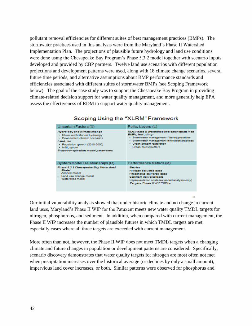
42

pollutant removal efficiencies for different suites of best management practices (BMPs). The

stormwater practices used in this analysis were from the Maryland’s Phase II Watershed

Implementation Plan. The projections of plausible future hydrology and land use conditions

were done using the Chesapeake Bay Program’s Phase 5.3.2 model together with scenario inputs

developed and provided by CBP partners. Twelve land use scenarios with different population

projections and development patterns were used, along with 18 climate change scenarios, several

future time periods, and alternative assumptions about BMP performance standards and

efficiencies associated with different suites of stormwater BMPs (see Scoping Framework

below). The goal of the case study was to support the Chesapeake Bay Program in providing

climate-related decision support for water quality management, and more generally help EPA

assess the effectiveness of RDM to support water quality management.

Our initial vulnerability analysis showed that under historic climate and no change in current

land uses, Maryland’s Phase II WIP for the Patuxent meets new water quality TMDL targets for

nitrogen, phosphorous, and sediment. In addition, when compared with current management, the

Phase II WIP increases the number of plausible futures in which TMDL targets are met,

especially cases where all three targets are exceeded with current management.

More often than not, however, the Phase II WIP does not meet TMDL targets when a changing

climate and future changes in population or development patterns are considered. Specifically,

scenario discovery demonstrates that water quality targets for nitrogen are most often not met

when precipitation increases over the historical average (or declines by only a small amount),

impervious land cover increases, or both. Similar patterns were observed for phosphorus and

43

sediment targets (see Figure below of Phase II Sediment and Nitrogen loads under different

combinations of climate and land use changes).

In the future, cost-effective options could be considered to hedge against future changes in

climate and land use. For example, greater investment in BMP types such as wetlands or urban

filtering practices may be considered that appear to provide cost-effective pollutant load

reduction for impervious areas when compared with other approaches.

However, a preliminary analysis suggests that in some plausible stressing futures, very few BMP

types considered could meet existing water quality targets at reasonable cost. This may mean

that additional options have to be developed and employed in the basin, including changes to

land use practices, to help avoid future impervious area growth. Also, developing “signposts” to

monitor to detect changes from the desired trajectory of control for pollutants could be used to

trigger additional BMP investments or new policy options. In general, monitoring BMPs, testing

current and potential new BMPs, adaptively managing as new data and information are gathered,

and revisiting targets where necessary are good practices in light of the significant climate

change uncertainties.

44

Approaches to the Simulation of Climate Change with the CBP Watershed and Estuarine

Model – Gopal Bhatt, PSU; Ping Wang, VIMS; and Guido Yactayo, UMCES

A collection of six General Circulation Models were used as inputs to estimate anticipated

changes in temperature throughout the watershed in the year 2050. Anticipated changes in

precipitation were adjusted by utilizing regressions derived from a 30 year historical record of

watershed precipitation events to extrapolate forward in time. Potential Evapotranspiration was

modified by Hamon’s method (1961) and increasing CO2 concentrations were used to effect

changes in stomatal resistance. These inputs resulted in large variations of watershed loadings in

comparison with loads generated from a calibration run of the Chesapeake Bay Program’s Phase

5.3.2 Watershed Model, suggesting that significant management actions would need to be taken

to account for steeply increasing nutrient and sediment loads anticipated for future climate

scenarios.

2017 Midpoint Assessment Management Needs – Lewis Linker, U.S. EPA Chesapeake Bay

Program and Carl Cerco, USACE-ERDC

Linker outlined the motivations and schedule demands that the Chesapeake Bay Program has

placed upon its decisions to integrate factors of altered climate in the Phase III Watershed

Implementation Plans (WIPs). The support systems in place to determine relative changes in

hypoxia and living resource conditions using the Bay Program’s Water Quality and Sediment

Transport Model (WQSTM) were also explained. Changes in water quality standards due to

impacts of changing temperature, sea-level, watershed loads, and tidal wetland attenuation were

discussed. Overall, there was generally little impact with regards to water quality standards from

these factors, although further exploration of these issues is necessary to better evaluate targeted

management responses to factors such as tidal marsh loss, stormwater management, or others.

Session III: Case-Study Examples of Climate Trend Assessments, Data, and Scenario

Needs for CBP Climate Assessments of Ecosystems

Downscaling Climate Models for Ecological Forecasting In Northeast U.S. Estuaries –

Barbara Muhling, Princeton/NOAA GFDL

Contributors: Barbara Muhling1,2, Carlos Gaitan2,3, Desiree Tommasi1,2 Charles Stock2, Vincent Saba2,4

Keith Dixon2 1: Princeton University Program in Atmospheric and Oceanic Sciences 2: NOAA Geophysical Fluid Dynamics Laboratory 3: University of Oklahoma 4: NOAA Northeast Fisheries Science Center

45

The objective of this project is to apply a range of statistical downscaling techniques to northeast

U.S. estuarine and nearshore environments, and to use these to project future habitat for

diadromous fishes and habitats. We are particularly interested in the contribution of the

downscaling method to overall uncertainty. Results presented here described the preliminary

application of these statistical techniques to the Chesapeake Bay and Susquehanna River

watershed.

Analyses of historical in situ observations showed that estuarine dynamics could be

approximated using only the atmospheric variables available from general circulation models (air

temperature, precipitation). An estuarine water temperature model was built using a non-linear

lagged air temperature relationship, and verified using >25 years of in situ measurements. A

water balance model using Hamon evapotranspiration was then applied to the Susquehanna

River watershed, which supplies ~50% of freshwater inflow to Chesapeake Bay. Historical

monthly river discharge (1970-2006) was well correlated with model predictions (R2=0.8), with

good bias characteristics once a correction for wind-induced snow under-catch was incorporated.

Air temperature over Chesapeake Bay, and air temperature and precipitation over the

Susquehanna watershed, were then downscaled using five different statistical techniques: bias

correction quantile mapping, change factor quantile mapping, equidistant quantile mapping,

cumulative distribution function transform, and a modified delta method. Projections from the

IPSL-CM5A-LR general circulation model (GCM) under RCP8.5 were selected for the initial

test case. Results showed that future modeled estuarine water temperatures from the downscaled

methods were cooler in spring, but warmer in summer than the GCM, with substantial (~2°C)

model spread at high temperatures. Similarly, the downscaled methods projected lower future

catchment precipitation and higher air temperatures than the GCM, resulting in lower calculated

Susquehanna River streamflow through 2100. Streamflow showed a slight negative trend

between the present day and 2100, but may have been biased by the use of a highly temperature-

dependent evapotranspiration metric. Overall, results suggested that use of different statistical

downscaling methods may have the greatest influence on projections once air temperatures

substantially exceed present day values, due to different ways of dealing with extrapolation

within each method. Ongoing work will apply downscaled projections to new and existing

models of distribution, recruitment and phenology for diadromous fishes and habitats.

Impacts of Climate Change on Chesapeake Oysters – Roger Mann and Ryan Carnegie,

Virginia Institute of Marine Science

Oysters (Crassostrea virginica) provide ecosystem services in the Chesapeake Bay as benthic

pelagic couplers, as structural complexity (reefs) in the benthos, and as a central component in

the bay alkalinity budget. All such services are subject to modification in response to projected

climate change. C. virginica occupies a remarkable latitudinal range from the Yucatan in the

south (annual temperature range 23.4 – 29.3oC) to Prince Edward Island in the north (annual

46

range -1.1 – 18.3oC); it is also found in a wide range of salinity from 5ppt in the upper

Chesapeake Bay to full seawater salinity in coastal embayments of the Atlantic coastline.

Projected climate driven temperature and salinity changes in the Chesapeake Bay are within

these ranges. The impact of resident oyster diseases (the non-native MSX and the native

Perkinsus marinus) is increased at higher temperature and salinity, and remains a long term point

of concern in bay oyster populations. Recent observations suggest that P. marinus is evolving in

response to competition with the introduced MSX, and the oyster is responding to both of these

changing disease challenges. Over the past decade the date of 50th percentile of oyster

recruitment has occurred increasingly earlier in the year, a movement in excess of 30 days in the

Piankatank and Great Wicomico Rivers, and slightly less so in the James River. In the

Piankatank and Great Wicomico Rivers the changing period of recruitment has resulted in a

larger mean size in Young of the Year (YOY) recruits in the fall months. Larger overwintering

YOY proffer the option of increased survival at the year one class, and gradually increasing rates

population expansion. In turn, increased production bodes well for shell accretion in reef

habitats and accumulation of carbonate as a component of the Bay-wide alkalinity bank. The

balance between recruitment, growth and mortality of live oysters, and the fate of shell as a

substrate is not a static equilibrium, but more appropriately described as a moving baseline.

What remains unresolved is (a) the question as to which of the complex climate drivers versus

non climate drivers dominate the observed changes, and (b) our ability to predict where this

movement will end.

Climate Change and Ecological Forecasting in the Chesapeake Bay – Howard Townsend,

NOAA

Beyond water quality, the Chesapeake Bay Program has a range of climate-related management

needs focused on habitats and living resources. To address these needs requires an

understanding of the effects of climate change at an ocean scale and estuarine scale. In the North

Atlantic, climate change is predicted to result in: 1) increased sea surface temperature and

surface salinity, 2) change in precipitation (resulting in salinity changes) and pH, as well as 3)

changes in peaks and timing of primary productivity. This wide-sweeping range of changes at

the ocean-scale becomes even more complex as we consider what might occur in the estuarine

environment with its multi-faceted habitats and variety of important living marine resources.

Given the wide array of changes and the complexity of the estuarine environment, assessing the

impacts of climate change on Chesapeake Bay habitats and living resources is a formidable task.

Working with partners, NOAA scientists have begun to make some initial attempts to assess

some of these climate impacts in the bay at an ecosystem-level down the level of pathogens.

This presentation highlighted some of these efforts, which although they are preliminary efforts,

they are important first steps.

47

Loss of Coastal Marshes to Sea-level Rise – Molly Mitchell, VIMS

Marshes contribute to habitat and water quality in the Chesapeake Bay. Their importance to Bay

functions has led to concerns about their persistence. In many areas, marshes are eroding, appear

to be disappearing through ponding in their interior or are being replaced with shoreline

stabilization structures. We undertook a study to examine the changes in marsh extent and

community over the past 40 years to better understand the effects of human pressure and sea-

level rise on marsh coverage.

Approximately 40 years ago, a tidal marsh inventory of the York River marshes established the

historic marsh communities and their distributions. This inventory was re-done in 2010 to

examine shifts in community composition, distribution and the extent of invasive species. Loss

of marsh was apparent throughout the mainstem of the York River, however, there was some

marsh gain near the turbidity maximum and where forested hummocks on marsh islands have

become inundated. Shifts in marsh community composition between historic and current

surveys were apparent although the type of shifts seen differed along the length of the river and

between the north and south shores. One significant change in marsh community has been the

introduction of Reedgrass (Phragmites australis) along the length of the York River. Indications

of marsh flooding (possibly due to sea-level rise) can be seen in the York River system where

areas which historically had significant high marsh communities appear to have converted almost

entirely to low marsh. Indications of salinity shifts can also be seen where historically

freshwater marshes now support brackish mixed communities.

Session IV: Climate Scenarios, Projections and Realizations

State Perspectives on Climate Change Scenario Selection – Kate Johnson, DC and Jennifer

DeMooy, DE

Delaware Climate Projections: Methods and Findings

Jennifer de Mooy (Delaware Division of Energy and Climate) presented a short summary of how

the state of Delaware had downscaled climate projections developed in 2012. The state’s interest

in having state-specific projections was driven in part by its coastal location and vulnerability to

storm surge, sea-level rise, and flooding.

Delaware contracted with Katharine Hayhoe, Anne Stoner, and Rodica Gelca from ATMOS

Research & Consulting to produce downscaled projections for temperature and precipitation

indicators. The Hayhoe proposal was selected for its use of both CMIP3 and CMIP5 models in

the analysis (CMIP5 models being new at the time). Dr. Hayhoe’s downscaling methodology –

48

Statistical Asynchronous Regional Regression Model (ARRM) – has been widely used in a

number of state, regional, and national assessments.

Delaware State Climatologist Daniel J. Leathers worked closely with Dr. Hayhoe’s team to

provide quality-controlled data from 14 Delaware weather stations. Local data is used in the

AARM statistical downscaling analysis. Dr. Leathers also conducted a review of historic trends

in temperature and precipitation, based on weather data from 1895 through 2012.

The projections analysis uses two scenarios: a higher and lower scenario corresponding with

RCP 8.5 (higher) and RCP 4.5 (lower), for a time frame through 2100. Over 160 climate

indicators were chosen for temperature, precipitation, and secondary indicators - relative

humidity, heat index, and potential evapotranspiration. These can generally be grouped by

averages and extremes. Averages include annual and seasonal averages, or percentage change;

extremes include number of days > or < certain thresholds (e.g. days with maximum temperature

>95˚F).

The methodology and findings of the climate projections analysis conducted for Delaware can be

found in the Delaware Climate Change Impact Assessment:

http://www.dnrec.delaware.gov/energy/Pages/The-Delaware-Climate-Impact-Assessment.aspx

To make the large volume of detailed data available to researchers and practitioners, the state of

Delaware has recently launched the Delaware Climate Projections Portal. Through the Portal,

projection data can be viewed or downloaded for any of the 14 weather stations for 55 climate

indicators and for any selection of years up to 2100. The Portal is still in beta-testing stage, but

can be accessed here: http://climate.udel.edu/declimateprojections/ . Please contact Jennifer de

Mooy with any questions. (Jennifer.Demooy@state.de.us)

Climate Change Projections for Washington, D.C.

Kate Johnson, with the Department of Energy and Environment (DOEE), presented an overview

of recently developed Climate Change Projections for Washington, DC. A recent study,

conducted Katharine Hayhoe and, Anne Stoner from ATMOS Research & Consulting, used

downscaling: a process of incorporating local data into global climate models in order to

translate the results to the local level. Nine global climate models were used along with high and

low emissions scenarios with local data from 3 weather stations. Daily temperature,

precipitation, and humidity projections for 1960‐ 2100 were produced for the study. Climate

projections were averaged over 20-year periods: Baseline (1981‐ 2000); 2020s (2015‐ 2034);

2050s (2045‐ 2064); and 2080s (2075‐ 2094). Climate indicators were then developed for the

following temperature and precipitation variables:

49

Precipitation (Extreme Events) Precipitation (Extreme Events) cont.

# of days/year with rainfall at or above 1 in 80th Percentile storm (in)

# of days/year with rainfall at or above 2 in 90th Percentile storm (in)

1‐yr 24 hr storm (in) 95th Percentile storm (in)

2‐yr 24 hr storm (in) Temperature (Average Temperature)

15‐yr 24 hr storm (in) Summer Maximum Temperature (daytime)

25‐yr 24 hr storm (in) Summer Minimum Temperature (nighttime)

100‐yr 24 hr storm (in) Extreme Events

200‐yr 24 hr storm (in) # of heat waves per year

2‐yr 6 hr storm (in) Avg heat wave duration (in days)

15‐yr 6 hr storm (in) # of days/yr with heat index at or above 95 F

100‐yr 6 hr storm (in) # of days/yr with ambient temp at or above 95 F

200‐yr 6 hr storm (in) Increase in frequency of the 2012 heat wave

The modeling also derived extreme heat events (expressed in days over 95°F heat index) and

looked at heat wave length and frequency. Heat waves, defined as 3 consecutive days when the

heat index is above 95°F, are projected to be more frequent and last longer. Results of modeling

for precipitation projections for DC indicate that observed trends in measures of extreme

precipitation are expected to continue to increase. Charts show the number of days per year with

more than 1” (top) and 2” (bottom) of precipitation in 24h. By the 2080s, the number of days per

year with more than 2” of rain are expected to more than double from 2 days to 4.5 days under

the higher scenario.

The project also included an analysis of “design storm” events. Changes in rainfall volumes

have a significant impact on infrastructure. Design storms are the selected events that engineers

use to design drainage infrastructure, bridges, culverts, etc. Input from DC Water, DDOT and

DDOE’s Stormwater Management Division informed the selection of events that are used as

standards for stormwater, wastewater, and transportation infrastructure. The chart below shows

how rainfall volumes are projected to increase across the relevant design storm events, especially

for the more extreme (100 and 200 year) events.

50

Johnson discussed how changes in design storm events presents both implications and

opportunities for further Modelling Drainage infrastructure is generally designed to handle

rainfall from a 15-year event. Historically, that meant 5.5” of rain. In the future, a storm with

the same frequency will bring rainfall of: 6.8” in the 2020s; 7.1” inches in the 2050s; and 8”

inches in the 2080s. The result, without upgrades, could mean more frequent flooding and CSO

discharges.

The Technical Report for the District of Columbia’s climate change projections can be found at:

http://doee.dc.gov/sites/default/files/dc/sites/ddoe/publication/attachments/Attachment%201%20

.ARC_.Report_07-10-2015.pdf

A Climate Scenario Selection Tool – Phil Morefield, U.S. EPA

There are numerous archives of climate model output freely available. The size, complexity and

diversity of data contained in these archives complicates the tasks of acquiring, processing and

then analyzing these model outputs. In addition, most of these archives provide little, if any,

guidance that helps answer the commonly asked question: “Which climate projection(s) should I

use?”

A new Web tool under development at EPA will assist interested users in the process of

identifying and processing climate model output. The LASSO project (Locating And Selecting

Scenarios Online) has two primary goals. First, to produce a simple, intuitive tool that provides

51

access to climate model output, with some ability to process that information into meaningful

statistics (e.g., seasonal climate deltas). Second, to provide a capability to visualize and explore

climate model output in a way that helps illuminate those climate realizations that might be most

useful to a particular user. The LASSO tool will present various strategies for selecting a

specific set of climate projections that generally reflect model uncertainty and risk tolerance in

the context of the user’s particular needs.