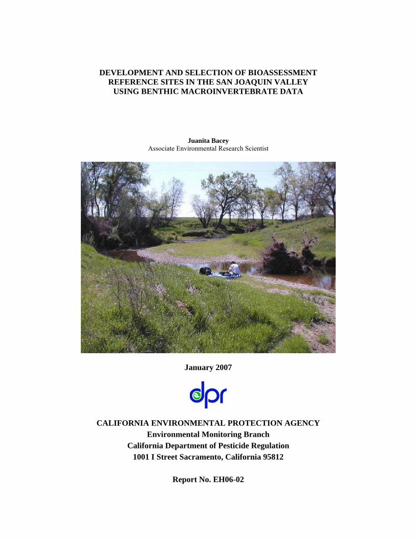
DEVELOPMENT AND SELECTION OF BIOASSESSMENT REFERENCE SITES IN THE SAN JOAQUIN VALLEY

USING BENTHIC MACROINVERTEBRATE DATA

Juanita Bacey Associate Environmental Research Scientist

January 2007

CALIFORNIA ENVIRONMENTAL PROTECTION AGENCY Environmental Monitoring Branch

California Department of Pesticide Regulation 1001 I Street Sacramento, California 95812

Report No. EH06-02

2

ABSTRACT A bioassessment reference is a segment of stream (reach) within an ecological region that represents a desired state or optimal condition of stream health. Often optimal conditions may be “best available” or “least impacted” within a region. The objective of this study was to develop a method for selecting benthic macroinvertebrate bioassessment reference sites in a low-gradient, anthropogenic-impacted region. Bioassessment reference sites for the San Joaquin Valley were selected using these criteria. Land use and pesticide use data as well as a variety of physical and chemical parameters known to affect the health of aquatic biological communities were examined. Sites were selected and benthic macroinvertebrates (BMIs) were collected. These BMIs represent the “expected” biological communities of “least impacted” wadable streams in the San Joaquin valley ecoregion. The pool of reference sites reflect a range of variability of biotic conditions, and offer a benchmark by which other sites in the ecoregion can be compared.

ACKNOWLEDGMENT DPR collaborated with the Central Valley Regional Water Quality Control Board (CVRWQCB) and the Department of Fish and Game (DFG) in development of this project. Technical contributions were also received from the State Water Resources Control Board (SWRCB), U.S. EPA and Dr. Lenwood W. Hall of the Wye Research and Education Center, University of Maryland. This project promoted cooperation between DPR and the SWRCB to protect water quality in accordance with the Management Agency Agreement that exists between the two agencies. We would like to thank the following environmental monitoring personnel who assisted with sample collection during the study: Adriana Moncada, Angela Csondes, Sheryl Gill, Keith Starner, Amrith Gunasekara, Milanka Ilic, and Michael Mamola. Their tireless efforts allow us to report the data presented here. Thanks also to the California Department of Food and Agriculture staff, Jane White, Jean Hsu and Hsiao Feng, who conducted chemical analysis, and the Bidwell Institute of California State University, Chico for benthic macroinvertebrate taxonomy.

3

TABLE OF CONTENTS Abstract……………………………………………………………………….…… ii Acknowledgment………………………………………………….……….……… ii Table of Contents …………………………………………………………….…… iii List of Tables ……………………………………………………………………… iii List of and Figures……………………………………………….………………… iii Introduction ………………………………………………………………….….… 1 Materials and Methods …………………………………………………………… 3 Selection of Reference sites……………………………………………..… 3 Method Development ……………………………………………………… 5

Sampling Methods………………………………………………………… 10 Analysis …………………………………………………..………….…… 10 Results and Discussion ……………………………………….…………….....….. 13 Conclusion ………………………………………………………….…………….. 17 References…………………………………………………………………………. 18 LIST OF TABLES Table 1. Selected pesticides used in the San Joaquin Valley 5 Table 2. Pesticides analyzed including methods, method limits, and

reporting limits 7 Table 3. Water quality and nutrient criteria 8 Table 4. Nutrient analysis methods 12 Table 5. Benthic macroinvertebrate metrics and definitions 13 Table 6. Water quality and nutrient criteria and detections 16 Table 7. Fraction of unionized ammonium in aqueous solution and different pH Values and temperatures 16 Table 8. Herbicide known LC50 values for aquatic organisms 17 Table 9. Water quality and pesticide results of final selected sites 26 Table 10. Pesticide results of final selected sites 27 Table 11. Benthic macroinvertebrate results of final selected sites 28 LIST OF FIGURES Figure 1. Surveyed area of the San Joaquin Valley ecoregion 4 Figure 2. Pesticide and land use along Little Johns Creek, San Joaquin County, California 9 Figure 3. Habitat assessment field data sheet 21-22 Figure 4. Physical characterization data sheet 23-24 Figure 5. Water quality field data sheet 25 Appendix 1. Pesticide analysis continuing quality control 29-34

4

I. INTRODUCTION There are over 200,000 miles of rivers and streams in California, and monitoring these waterways for pollutants is the responsibility of many state and local government agencies. The California Department of Pesticide Regulation (DPR) monitors for the occurrence of pesticides in surface water, as well as in ground water and air. Economic and logistical constraints allow only periodic monitoring of select surface waters. Monitoring is often limited to those areas with the highest levels of surrounding pesticide use and therefore the most likely to be impacted. Pesticide inputs to surface water commonly occur as pulses and may be missed with occasional monitoring. Additionally, chemical analysis is often limited to certain pesticides. However, not all pesticides that enter surface waters impact the aquatic biota. Some pesticides are hydrophobic and they bind quickly to sediments or other organic matter in water. This reduces the bioavailability of these pesticides to aquatic organisms in the water column. However, benthic macroinvertebrates (BMIs) that reside in the interstitial waters between cobble and other substrates may be impacted by pesticide-laden sediment. Acute and chronic water and sediment toxicity tests are additional monitoring tools. However, these tests only take into consideration the toxicity of pesticides found in a sample collected at that moment in time, and do not consider the movement, fate, and bioaccumulation of pesticides in the environment. These tests do not determine impacts to the biological community but generally to just one test species. They also do not assess integrated ecological impacts to biota from multiple stressors such as low dissolved oxygen levels, warm temperatures, and decreased physical habitat. Though the chronic risk to the aquatic biota from pesticides is uncertain, some pesticides along with other anthropogenic factors have a high potential for enhancing toxicity in aquatic biological communities. Over the last several decades zooplankton, cladoceran, and benthic invertebrate populations have declined in the Sacramento-San Joaquin Basins, Delta, and San Francisco estuary. It has been suggested that one factor is the presence of pesticides in surface waters (Obrebski et al., 1992; Cooke et al., 1999). Invertebrate populations are a necessary food source for nearly all fish populations in the Sacramento-San Joaquin basins during their early life stages (Moyle et al., 1996; Meng and Moyle, 1996). Consequently, a decline in aquatic invertebrate populations may lead to a decline in fish populations. Determining the biological integrity or current condition of a water body is challenging due to the magnitude of anthropogenic activities influencing California waterways. Biological integrity as defined by the U.S. EPA is “the ability of an aquatic ecosystem to support and maintain a balanced, integrated, adaptive community of organisms having a species composition, diversity and functional organization comparable to that of the natural habitats of a region.”

5

Conducting an assessment of an aquatic biological community (e.g. insects, fish, plant life), also known as bioassessment, can assist in the determination of a water body’s biological integrity. One biological community most often monitored in bioassessment studies is BMIs. BMIs are ubiquitous, complete the majority of their life cycle in water, and are relatively stationary. They are useful in evaluating water quality and the overall health of a water system in flowing waters because they are affected by changes in a stream’s chemical and/or physical structure (Karr and Kerans, 1991). Their large species diversity also provides a range of responses to environmental stresses (Rosenberg and Resh, 1993). All of these characteristics allow them to be effective indicators of specific anthropogenic disturbances (House et al., 1993), cumulative effects of multiple stressors, and the historical conditions of a water body (Friedrich et al., 1992). Once bioassessment has been conducted, results can be compared to a reference to determine the biological integrity. A bioassessment reference is a stream reach within an ecoregion that represents a desired state or optimal condition of stream health. Often optimal conditions may be “best available” or “least impacted” within a region; as such, they can represent a benchmark by which other locations within that region can be compared. A pool of reference sites provides a range in variability of biotic conditions. The purpose of this study was to develop an objective, quantitative method for identifying and selecting reference sites in the San Joaquin Valley watershed region or any similar low elevation, low-gradient (< 2% slope), anthropogenic impacted region. The objective was to select a pool of 100 potential sites and conduct physical habitat and chemical assessments. The 30 “best available” sites would be selected from this pool. BMI’s would be collected from these final 30 sites. These could then be used for future comparisons with samples collected from other streams within this ecoregion.

2. Materials and Methods

Study Area The area of interest is the low-gradient, San Joaquin Valley ecoregion. The initial step in selecting reference sites was to define the region’s boundaries and the stream types that should be evaluated. The boundaries included a portion or all of the following Sacramento and San Joaquin central valley hydrobasins in the state of California, as defined by the CVRWQCB (ISWP, 1991): 32 – East of the Delta, 35A – Turlock, 35B – Merced, 40 – Westside San Joaquin River, 41 – Grasslands, 44A – Central Delta, 44C – South Delta, 45 – San Joaquin Valley floor (Figure 1). These hydrobasins encompass the San Joaquin River watershed. East and west boundaries did not exceed 250 feet (76m) in elevation in order to stay within the low gradient ecoregion. As elevation changes so does the ecoregion and biological community; therefore, a bioassessment reference site for one ecoregion could not represent a reference site for another ecoregion.

6

The selected area included perennial streams and those “natural channel” streams dominated by agricultural supply water as determined by the CVRWQCB (ISWP, 1991). Those dominated by agricultural and/or urban drainage waters were not considered due to the possible input of multiple pollutants (e.g. pesticides, metals, oils, detergents). All streams examined were first and second order streams. Due to growing urban sprawl and extensive agricultural activities within the San Joaquin Valley, water hydrology has been greatly modified, and water quality has been impacted by pollutant runoff (e.g. sediment, pesticides, nutrients). Therefore, stream reaches within this ecoregion were evaluated for “least impacted” conditions. A variety of parameters known to affect the health of aquatic biological communities were measured. These included physical habitat, nutrients, and basic water quality. Water quality measurements were compared to EPA standards or known water quality criteria, and land and pesticide uses surrounding waterways were also examined. Those stream sites with the “least impacted” anthropogenic conditions were selected as the final reference sites.

7

Figure 1. Surveyed area of the San Joaquin Valley ecoregion

Note: This map does not include all streams surveyed in the ecoregion due to the size of the map displayed here.

8

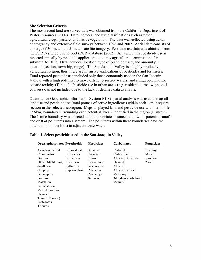
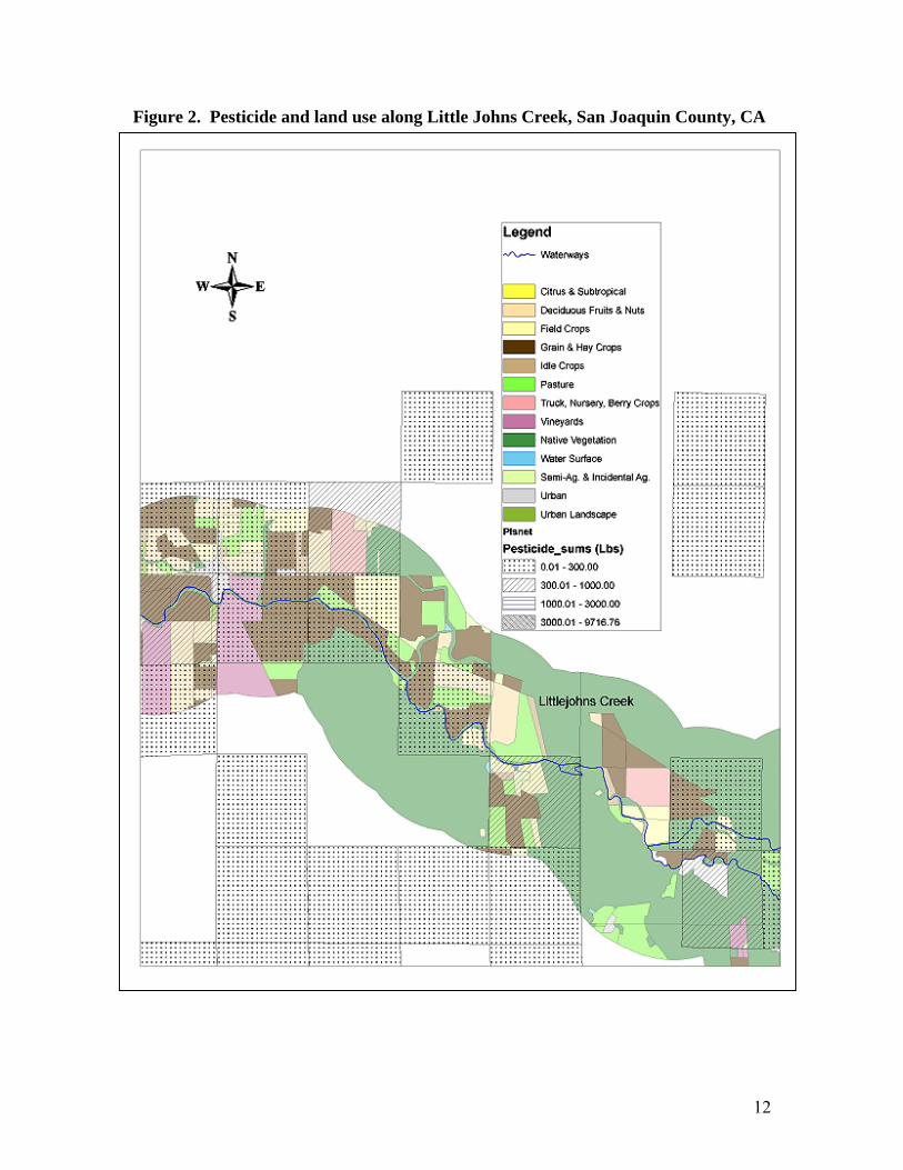
Site Selection Criteria The most recent land use survey data was obtained from the California Department of Water Resources (2002). Data includes land use classifications such as urban, agricultural crops, pasture, and native vegetation. The data was collected using aerial photography and extensive field surveys between 1996 and 2002. Aerial data consists of a merge of 30-meter and 5-meter satellite imagery. Pesticide use data was obtained from the DPR Pesticide Use Report (PUR) database (2002). All agricultural pesticide use is reported annually by pesticide applicators to county agricultural commissions for submittal to DPR. Data includes: location, type of pesticide used, and amount per location (section, township, range). The San Joaquin Valley is a highly productive agricultural region; thus, there are intensive applications of pesticides and fertilizers. Total reported pesticide use included only those commonly used in the San Joaquin Valley, with a high potential to move offsite to surface waters, and a high potential for aquatic toxicity (Table 1). Pesticide use in urban areas (e.g. residential, roadways, golf courses) was not included due to the lack of detailed data available. Quantitative Geographic Information System (GIS) spatial analysis was used to map all land use and pesticide use (total pounds of active ingredients) within each 1-mile square section in the selected ecoregion. Maps displayed land and pesticide use within a 1-mile (2.6km) boundary surrounding each potential stream identified in the region (Figure 2). The 1-mile boundary was selected as an appropriate distance to allow for potential runoff and drift of pollutants into a stream. The pollutants within these boundaries have the potential to impact biota in adjacent waterways. Table 1. Select pesticide used in the San Joaquin Valley

Organophosphates Pyrethroids Herbicides Carbamates Fungicides

Azinphos methyl Esfenvalerate Atrazine Carbaryl Benomyl Chlorpyrifos Fenvalerate Bromacil Carbofuran Maneb Diazinon Permethrin Diuron Aldicarb Sulfoxide Iprodione DDVP (dichlorvos) Bifenthrin Hexazinone Oxamyl Ziram disulfoton Cyfluthrin Norflurazon Aldicarb ethoprop Cypermethrin Prometon Aldicarb Sulfone Fenamiphos Prometryn Methomyl Fonofos Simazine 3-Hydroxycarbofuran Malathion Mesurol methidathion Methyl Parathion Phosmet Thimet (Phorate) Profenofos Tribufos

9

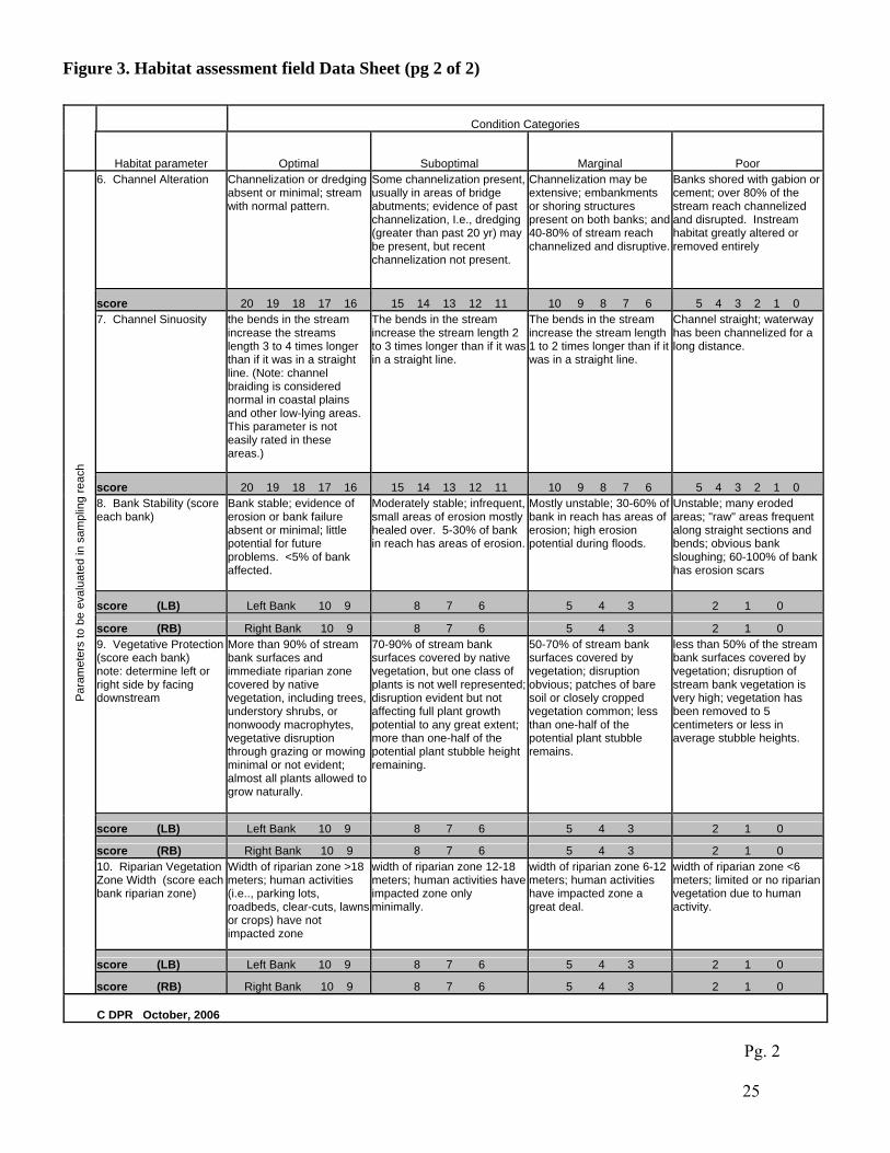
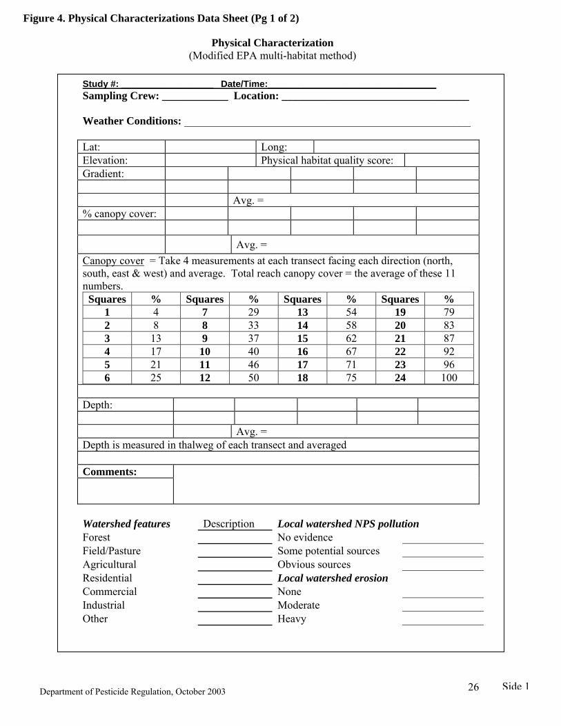
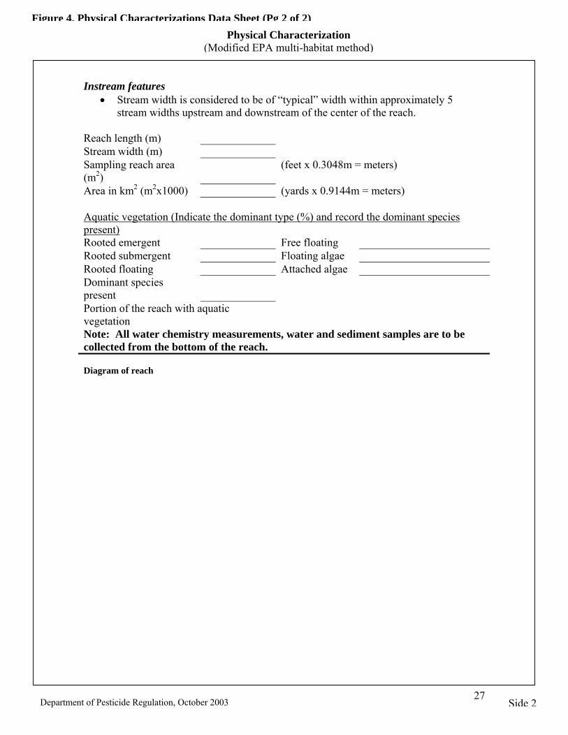
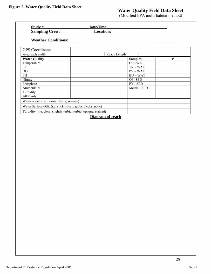
Next, due to the fact that current land and pesticide use data was not available, potential sites were visually surveyed to verify surrounding land use and water flow. Properties directly adjacent to streams were identified with county assessor parcel maps, and property owners were contacted to access private properties. Site surveys consisted of visual inspections of the stream reach, adjacent riparian fauna, surrounding anthropogenic activities, and accessibility. Stream sites that had been altered and had visibly poor physical habitat characteristics were eliminated (e.g. channelized streams, lack of riparian vegetation). The initial pesticide criterion was set so that those sections of streams that were surrounded by greater than 100 pounds of pesticide use in a one-year period would be eliminated. Site-surveys revealed either greater agricultural production or urban expansion than shown on pesticide and land use data maps, and revealed additional anthropogenic impacts to surface waters. Therefore, in order to increase the pool of potential reference sites, the pesticide criterion was increased to include those reaches of streams that had greater than 100 pounds of surrounding pesticide use, but less than 1000 pounds in a one-year period. Those sections that had high population densities (cities/towns) were eliminated due to the possible input of multiple, urban pollutants (e.g. pesticides, petroleum by products, detergents). Over 300 sites from 32 streams were site-surveyed and/or considered in the region. Of those sites, 26 were found to meet the final land use and pesticide use criteria. Water quality and physical habitat assessments were conducted at the 26 sites within a defined reach of the stream. Each reach was determined as the average width of the stream times 40, and was limited to a minimum of 150 meters and a maximum of 500 meters (U.S. EPA, 2001). The physical habitat assessment consisted of completing a Habitat Assessment Field Data Sheet for low gradient streams (Figure 3). The U.S. EPA defined the physical habitat scoring criteria (1999). A score is determined by assessing 10 physical habitat characteristics that include in-stream features (e.g. undercut banks, pools, channel flow and alteration) and riparian composition along the stream bank and beyond. Each of the 10 characteristics is valued at 20 points. Total scores can range from 0 to 200 with 0 representing significant anthropogenic or natural impacts and 200 representing no impacts. These scores are an observation-based score and can be subjective due to the experience or background of the individual conducting the assessment. Therefore, the score is usually determined by consensus of three or more field staff. The water quality assessment entailed completing a modified U.S. EPA Physical Characterization data sheet and a Water Quality Field data sheet (Figure 4-5). These data sheets included basic water quality parameters that were measured in situ (temperature, pH, dissolved oxygen, specific conductance, turbidity) and select nutrients (nitrate, phosphate, ammonium nitrogen, alkalinity). Additional in-stream physical habitat parameters were also measured (percent gradient, percent canopy cover, average depth, turbidity, substrate particle size and percent substrate embeddedness).

10

Both substrate type and substrate embeddedness were determined by visually inspecting substrate at 55 points within the stream reach following a modified U.S. EPA method (DPR, 2004). Samples were also collected and analyzed for select herbicides, organophosphate and pyrethroid insecticides in water, and pyrethroid insecticides in sediment (Table 2). Table 2. Pesticides analyzed including methods, method limits and reporting limits

Organophosphate Pesticides in Water Method: GC/FPD

Triazines/Herbicides in Water Method: APCI/LC/MS/MS

Compound Method Detection Limit (ppb)

Reporting Limit (ppb)

Compound Method Detection Limit (ppb)

Reporting Limit (ppb)

Azinphos methyl 0.0099 0.05 Atrazine 0.02 0.05 DDVP (dichlorvos) 0.0098 0.05 Bromacil 0.031 0.05 Dimethoate 0.0079 0.04 Diuron 0.022 0.05 Disulfoton 0.0093 0.04 Hexazinone 0.04 0.05 Ethoprop 0.0098 0.05 Metribuzin 0.025 0.05 Fenamiphos 0.0125 0.019 0.05 Fonofos 0.008

0.05 0.04

Norflurazon Prometon 0.016 0.05

Malathion 0.0117 0.04 Prometryn 0.016 0.05 Methidathion 0.0111 0.05 Simazine 0.013 0.05 Methyl Parathion 0.008 0.03 DEA 0.010 0.05 Thimet (Phorate) 0.0083 0.05 ACET 0.030 0.05 Profenofos 0.0114 0.05 DACT 0.016 0.05 Tribufos 0.0142 0.05 GC/MS ppt ppt Chlorpyrifos 0.7999 10 Diazinon 0.191 10 Pyrethroid Pesticides in Surface Water -- Method: GC/MSD Compound Method Detection Limit (ppt) Reporting Limit (ppt) Fenvalerate/Esfenvalerate 22.5 50 Permethrin 16.9 50 Bifenthrin 2.16 5 Lambda Cyhalothrin 7.76 20 Cyfluthrin 55.5 80 Cypermethrin 56.6 80 Pyrethroid Pesticides in Sediment -- Method: GC/ECD, confirmed with GC/MSD (ppm) (ppm) Fenvalerate/Esfenvalerate 0.008 0.010 Permethrin 0.006 0.010 Bifenthrin 0.007 0.010 Lambda Cyhalothrin 0.009 0.010 Cyfluthrin 0.008 0.010 Cypermethrin 0.008 0.010

11

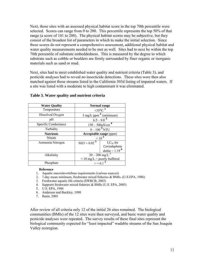
Next, those sites with an assessed physical habitat score in the top 70th percentile were selected. Scores can range from 0 to 200. This percentile represents the top 50% of that range (a score of 101 to 200). The physical habitat scores may be subjective, but they consist of the broadest list of parameters in which to make the initial selection. Since these scores do not represent a comprehensive assessment, additional physical habitat and water quality measurements needed to be met as well. Sites had to next be within the top 70th percentile of substrate embeddedness. This is measured by the degree to which substrate such as cobble or boulders are firmly surrounded by finer organic or inorganic materials such as sand or mud. Next, sites had to meet established water quality and nutrient criteria (Table 3), and pesticide analyses had to reveal no insecticide detections. These sites were then also matched against those streams listed in the California 303d listing of impaired waters. If a site was listed with a moderate to high contaminant it was eliminated. Table 3. Water quality and nutrient criteria

Reference 1. Aquatic macroinvertebrae requirements (various sources) 2. 7-day mean minimum, freshwater mixed fisheries & BMIs. (U.S.EPA, 1986) 3. Freshwater aquatic life criteria (SWRCB, 2003) 4. Supports freshwater mixed fisheries & BMIs (U.S. EPA, 2005) 5. U.S. EPA, 1986 6. Anderson and Buckley, 1998 7. Basin, 2005

After review of all criteria only 12 of the initial 26 sites remained. The biological communities (BMIs) of the 12 sites were then surveyed, and basic water quality and pesticide analyses were repeated. The survey results of these final sites represent the biological community expected for “least impacted” wadable streams of the San Joaquin Valley ecoregion.

Water Quality Normal range Temperature <35oC 1

Dissolved Oxygen 5 mg/L ppm 2 (minimum) pH 6.5 – 9.0 3

Specific Conductance 150 – 500μS/cm 4 Turbidity 0 – 100 3 NTU Nutrients Acceptable range (ppm)

Nitrate < 10 5 Ammonia Nitrogen NH3 < 0.02 5 LC50 for

Ceriodaphnia dubia = 1.19 6

Alkalinity 20 – 200 mg/L 7 < 10 mg/L = poorly buffered

Phosphate < = 0.1 5

12

Figure 2. Pesticide and land use along Little Johns Creek, San Joaquin County, CA

13

Sampling Methods Water Sampling Water samples for pesticide analyses were individually collected in 1-liter amber glass bottles from as close to center channel as possible below the surface of the water, and sealed with Teflon-lined lids. Samples were transported on wet ice then stored refrigerated at 4oC until extraction for chemical analysis. Water samples for nutrient analysis were individually collected in 10-ml glass vials and analyses were conducted at the sampling site. Sediment Sampling One sediment sample was collected from each site using a 24-inch long, 2-inch diameter, polycarbonate cylinder tube. One end of the tube was thrust into the sediment and then removed. The top 2.0 cm of the sediment collected in the tube was placed into a clear 1-pint glass jar. This was repeated approximately five times in the same general area and composited. Samples were transported on wet ice, then stored frozen at –14oC until extraction for chemical analysis. Benthic Macroinvertebrate Sampling Benthic macroinvertebrate sampling was conducted using a modified U.S. EPA Environmental Monitoring and Assessment Program method (DPR, 2004). This method was modified by DPR for use in a low-gradient, high anthropogenic region, from the U.S. EPA’s Surface Waters: Western Pilot Study Field Operations Manual for Wadable Streams (U.S. EPA, 2001). Quality Control and Analyses Pesticide Analyses The California Department of Food and Agriculture Center for Analytical Chemistry performed pesticide chemical analyses for all water and sediment samples. Quality control was conducted in accordance with standard Department of Pesticide Regulation QC procedures (Segawa, 1995), and included approximately 5% of samples as blind spikes. Samples with no residue above the MDL were reported as non-detections. Samples with a residue concentration that fell between the RL and the MDL were reported as trace detections. The analytical chemist used his/her best professional judgment to make this determination. Samples with residues above the RL were considered detections and analytical concentrations were reported. Pyrethroid whole water samples, including any suspended sediment, were extracted in toto with methylene chloride. Sample bottles were rinsed with extraction solvent and added to the sample extracts for analysis. The extract was passed through sodium sulfate to remove residual water. The anhydrous extract was evaporated on a rotary evaporator and then a solvent exchange performed with hexane. Extracts were concentrated using a Brinkmann R110 rotary evaporator (Brinkmann, Westbury, NY), and analyzed using a gas chromatograph (GC) equipped with a mass selective detector. Pyrethroid analysis results are reported on a whole water basis (water plus suspended sediment). Reporting limits were 5 to 80 ppt

14

Pyrethroid sediment samples were homogenized and extracted with acetonitrile. The filtered extracts were salted out with sodium chloride. An aliquot of acetonitrile extract was evaporated to dryness in a water bath under a stream of nitrogen for solvent exchange to hexane. Extracts were analyzed using GC with electron capture detector (ECD), and were confirmed using GC equipped with a mass selective detector. Reporting limits were 0.01 ppm. Organophosphate samples were extracted with methylene chloride and the extract was passed through sodium sulfate to remove residual water. The anhydrous extract was evaporated to near dryness on a rotary evaporator and diluted to a final volume of 1.0 mL with acetone. The extract was then analyzed by a GC equipped with an Rtx OP Pesticides column (Restek State College, PA) and a flame photometric detector (FPD). Reporting limits were 0.03 to 0.05 ppb. The same extract was analyzed by another GC with a 5% phenyl methylsilicone fused silica column (Hewlett Packard-5ms or equivalent) and a MSD, to determine the lower chlorpyrifos and diazinon results. The reporting limits for chlorpyrifos and diazinon are both 10 ppt. For herbicide analyses, the water samples were passed through two Oasis MCX cartridges (Waters, Millford, MA) connected in tandem. The cartridges were then eluted under vacuum with 5% ammonium hydroxide in methanol. The eluant was filtered through a nylon Acrodisc 0.2-micron filter (Gelman Sciences, Ann Arbor, MI), concentrated, reconstituted in 75/25 water/methanol, and analyzed by a liquid chromatography, a C18 column and atmospheric pressure chemical ionization mass spectrometry (APCI/LC/MS/MS). Reporting limits were 0.05 ppb. Nutrient and Other Analysis Field staff conducted the following analyses using field LaMotte Smart II® colorimeters: turbidity, alkalinity, nitrate, phosphate, and ammonium nitrogen. With the exception of turbidity, all samples were filtered immediately after collection using a disposable, sterile, polypropylene/polyethylene syringe and a Luer-Lok® sterile, surfactant-free, cellulose acetate membrane filter (0.45μm). Smart II colorimeters photoelectrically measure the amount of colored light absorbed by a colored sample in reference to a colorless sample (blank). Samples are reacted to produce a color by adding a reagent. Reagents were added and samples were measured in accordance with the LaMotte Smart II® test instructions (Table 4). Benthic Macroinvertebrate Identification The Bidwell Environmental Institute of California State University, Chico conducted identification of BMIs. Quality control was conducted in accordance with previously established California Department of Fish and Game procedures. For analysis of each sample a random sub-sample of 500 macroinvertebrates was identified as to genera, and when possible, to species. Taxa are then summarized into biological metrics (Table 5).

15

GIS Analysis GIS spatial analysis was used to map all land and pesticide use in the central valley ecoregion (ArcView ver. 3.2). Twelve categories of land use were displayed, while pesticides are displayed as ranges of total pounds of active ingredient used in a square mile section (section, township, range). Pesticide use ranges were 0-100 pounds, 101-1000 pounds, 1001-3000 pounds, and > 3001 pounds. All data is further modified to display only use within a 1-mile boundary surrounding each stream in the ecoregion (Figure 2). Table 4. Nutrient analysis methods Analyte Detection Limit Colorimeter range Method Alkalinity 10.0ppm 0-200 ppm as CaCO3 The sample is added to a buffered indicator reagent.

The color that develops will indicate the amount of alkalinity in the sample.

Ammonia-Nitrogen

0.05ppm 0.00 – 4.00 ppm Ammonia Nitrogen

Ammonia forms a colored complex with Nessler’s Reagent in proportion to the amount of ammonia present in the sample. Rochelle salt is added to prevent precipitation of calcium or magnesium in undistilled samples.

Nitrate 5.0ppm 0.0 – 60.0 ppm Zinc is used to reduce nitrate to nitrite. The nitrite that was originally present, plus the reduced nitrate, reacts with chromotropic acid to form a red color in proportion to the amount of nitrite in the sample.

Phosphate 0.05ppm 0.00 – 3.00 ppm Orthophosphate

Ammonium molybdate and antimony potassium tartrate react in a filtered acid medium with dilute solution of PO4

-3 to form an antimony-phosphomolybdate complex. This complex is reduced to an intense blue colored complex by ascorbic acid. The color is proportional to the amount of phosphate present.

Turbidity 2 NTU 0 – 400 NTU Absorptimetric

16

Table 5. Benthic macroinvertebrate metrics and definitions

Abundance Estimated number of BMIs in the sample calculated by extrapolating from the proportion of organisms counted in the subsample.

Taxonomic Richness Total number of individual taxa Tolerance Value Value between 0 and 10 weighted for abundance of individuals

designated as pollution tolerant (higher values) and intolerant (lower values)

Tolerant Taxa Taxon-specific organisms in sample that are highly tolerant to impairment as indicated by a tolerance value of 8 through 10

Intolerant Taxa Organisms in sample that are highly intolerant to impairment as indicated by a tolerance value of 0 through 2

Percent Dominant Taxon Percent of organisms in sample that is the single most abundant taxon EPT Taxa Number of families in the Ephemeroptera (mayfly), Plecoptera

(stonefly) and Trichoptera (caddisfly) insect orders Gatherers BMIs that collect or gather fine particulate matter Filterers BMIs that filter fine particulate matter Scrapers BMIs that graze upon periphyton Predators BMIs that feed on other organisms Shredders BMIs that shred coarse particulate matter The Tolerance Value reflects a community level tolerance. This metric was originally designed to serve as a measure of community tolerance to organic pollution (decaying plants and animals, manure, sewage). The regionally specific tolerance values for BMI communities in the Pacific Northwest are used here (CAMLnet, 2003). In addition, the EPA has established a list of tolerance values applicable to BMI communities in the northwestern U.S. based on their bioassessment program in Idaho. If a taxon found in California is not assigned a value in the Pacific Northwest, then this EPA value is used. A moderately disturbed stream typically has a tolerance value in the mid-range values (Harrington and Born, 1999). The Functional Feeding Groups (collectors, filterers, etc.) represent the processes or feeding habits of different macroinvertebrates in the stream. They also represent ecology production and food source availability within the stream. An imbalance of the feeding groups may reflect an unstable food process and indicate a stressed condition (Harrington and Born, 1999).

Modified from Harrington and Born, 1999

3. Results and Discussion

Over 300 sites from 32 streams were site-surveyed and/or considered in the region. Of those sites only 26 met pesticide and land use criteria. Although this was far fewer than the initial objective of 100, pesticide and physical habitat criteria were not relaxed. This would have increased pesticide and other pollutant inputs from higher population density areas, and lowered the benchmark to an unacceptable level. Physical habitat and water quality assessments were conducted at these 26 sites. This data was used to select the final sites. Physical habitat assessment scores ranged from 29 to 165. Those sites with a score in the top 70th percentile were selected (>100). These scores alone are not sufficient to characterize a site; therefore, additional measurable parameters were used to select the final sites.

17

These parameters were substrate embeddedness, basic water quality, nutrient criteria, and the absence of pesticide detections. Although flow can be a major stressor to aquatic life, this data was not available and therefore unable to be used as a selection factor. Canopy coverage was measured at each site but was also not used as a selection factor. Zimmerman and Death (2002) found that artificial cover over rock baskets in a natural stream had no effect on overall abundance and species richness. Giffith el al. (2002) tried to determine BMI metrics that would assess a relationship between canopy coverage and found no metric they tested correlated well. In this study coverage over the width of the streams ranged from 2 to 95%. Heavy sedimentation within a stream will decrease insect diversity and growth (Resh and Rosenberg, 1993); therefore, substrate embeddedness was used as the secondary selection factor in the selection of the final sites. All sites within the top 70% of least embeddedness were initially selected. Substrate embeddedness ranged from 14 to 100%. Substrate of a stream can consist of inorganic matter (large boulders, cobble of various sizes, gravel, sand, fine silt or mud, clay) and particulate organic matter (detritus). Substrate type is important because many pollution intolerant taxa require open interstitial spaces in the substrate. Chambers and Messinger (2001) found the numbers of Ephemeroptera, Plecoptera and Trichoptera taxa (EPT; pollutant intolerant taxa) in a sample were positively correlated with median particle size. However, substrate type was not used as a selection factor in this study due to the high percentage of embeddedness at all sites. Seventy-seven percent of the sites were 50% or greater embedded with fine silt, mud or sand. Next, sites had to meet basic water quality criteria for aquatic life (Table 3). Water quality sampling was limited to two events, the initial survey, and again at the time of BMI sampling. The data are presented here to show water quality conditions during those times only and to indicate potential impacts to BMIs (Table 6). Due to the limited number of measurements collected, criteria were used as a guide only. Dissolved oxygen concentrations at all sites except one (4.52 ppm) met the U.S. EPA (1986) national warm water quality criterion of greater than or equal to 5 mg/L (ppm). This site was not included in the final selected sites. The SWRCB freshwater aquatic life criterion for pH is 6.5 to 9.0 (2003). All but one site met this criterion (6.13). Follow-up pH measurements at this site were within normal ranges therefore this site was not eliminated. All sites fell within the California fresh water aquatic life criterion for turbidity (0-100 NTU; SWRCB, 2003). Measurements ranged from 0 - 39 NTU. Conductivity generally ranges from 50 to 1500 µS/cm in rivers of the United States. Streams supporting good mixed fisheries generally have a range between 150 to 500μS/cm, and those outside this range may not be suitable for certain species of fish or macroinvertebrates (U.S. EPA, 2005). Of the 26 potential sites, three were below this guideline (37.8 - 87.9 μS/cm), while four were above (681 - 1174 μs/cm). Historical natural conditions of those sites on the west

18

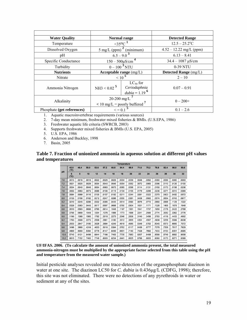
that flow east into the San Joaquin River generally have conductivity levels over 500 μS/cm. Therefore, due to the variability of conductivity levels in the ecoregion conductivity was not used as a selection factor. Total ammonia-nitrogen ranged from 0.1 to 2.90 mg/L (ppm). Total ammonia-nitrogen was converted to unionized-ammonia (NH3) using Table 7. This is the principal toxic form of ammonia. The U.S.EPA criterion for NH3 is < 0.02mg/L (ppm) for which all aquatic life may be protected (1986). Measured NH3 concentrations in this study ranged from 0.001 to 0.028 ppm. The concentration of NH3 is dependent on pH and temperature; therefore, ammonia toxicity varies with pH and temperature. Due to the imprecision of the conversion table, the highest multiplier was used when making conversions to NH3, thus, calculated concentrations may be higher than actual conditions. Therefore, those sites with concentrations that exceeded 0.02 ppm but were less than 0.03 ppm NH3 were not eliminated. The national drinking water standard for nitrate must be no greater than 10mg/L (ppm). This is also the ambient standard to protect aquatic ecosystems as well (U.S.EPA, 1986). None of the 26 potential sites exceeded this criterion. Concentrations ranged from 2 – 10 ppm. Alkalinity is a measure of the buffering capacity of water to neutralize acids. It refers to the ability of water to resist change in pH. Waters high in alkalinity (100-200 mg/L) can resist major changes in pH, and therefore protect aquatic life from acidic shock. Due to differences in geology, alkalinity levels can vary widely. Levels in fresh water generally range from 20-200 mg/L. Levels below 10 mg/L may indicate the system is poorly buffered (Basin, 2005). Only two of the 26 potential sites had levels below 10 mg/L and one was above 200 mg/L. These three sites were not included in the final selection of sites. Phosphate was measured as orthophosphate (dissolved phosphorus), the portion readily available to plants and algae. The U.S. EPA (1986) criterion is < 0.1 mg/L (ppm) in streams or flowing waters that do not discharge into lakes or reservoirs, so as to control algal growth. Phosphate concentrations were above this level in all but one of the 26 sites (0.008 ppm). Therefore, phosphate was not used as a selection factor. Table 6. Water quality and nutrient detections and criteria

19

1. Aquatic macroinvertebrae requirements (various sources) 2. 7-day mean minimum, freshwater mixed fisheries & BMIs. (U.S.EPA, 1986) 3. Freshwater aquatic life criteria (SWRCB, 2003) 4. Supports freshwater mixed fisheries & BMIs (U.S. EPA, 2005) 5. U.S. EPA, 1986 6. Anderson and Buckley, 1998 7. Basin, 2005

Table 7. Fraction of unionized ammonia in aqueous solution at different pH values and temperatures

UF/IFAS. 2006. (To calculate the amount of unionized ammonia present, the total measured ammonia-nitrogen must be multiplied by the appropriate factor selected from this table using the pH and temperature from the measured water sample.) Initial pesticide analyses revealed one trace-detection of the organophosphate diazinon in water at one site. The diazinon LC50 for C. dubia is 0.436μg/L (CDFG, 1998); therefore, this site was not eliminated. There were no detections of any pyrethroids in water or sediment at any of the sites.

Water Quality Normal range Detected Range

Temperature <35oC 1 12.5 – 25.2oC Dissolved Oxygen 5 mg/L (ppm) 2 (minimum) 4.52 – 12.22 mg/L (ppm)

pH 6.5 – 9.0 3 6.13 – 8.41 Specific Conductance 150 – 500μS/cm 4 34.4 – 1087 μS/cm

Turbidity 0 – 100 3 NTU 0-39 NTU Nutrients Acceptable range (mg/L) Detected Range (mg/L)

Nitrate < 10 5 2 – 10

Ammonia Nitrogen NH3 < 0.02 5 LC50 for

Ceriodaphnia dubia = 1.19 6

0.07 – 0.91

Alkalinity 20-200 mg/L 7

< 10 mg/L = poorly buffered 7 0 – 200+

Phosphate (get references) < = 0.1 5 0.1 – 2.6

20

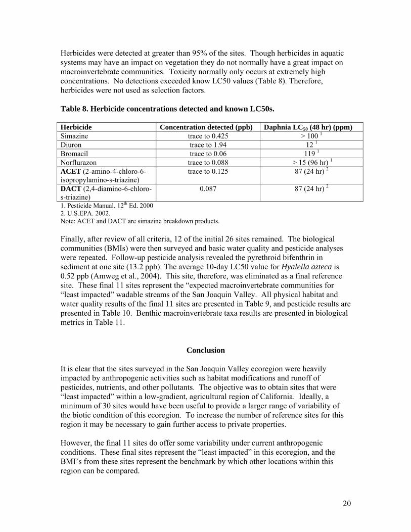
Herbicides were detected at greater than 95% of the sites. Though herbicides in aquatic systems may have an impact on vegetation they do not normally have a great impact on macroinvertebrate communities. Toxicity normally only occurs at extremely high concentrations. No detections exceeded know LC50 values (Table 8). Therefore, herbicides were not used as selection factors. Table 8. Herbicide concentrations detected and known LC50s. Herbicide Concentration detected (ppb) Daphnia LC50 (48 hr) (ppm) Simazine trace to 0.425 > 100 1 Diuron trace to 1.94 12 1 Bromacil trace to 0.06 119 1 Norflurazon trace to 0.088 > 15 (96 hr) 1 ACET (2-amino-4-chloro-6-isopropylamino-s-triazine)

trace to 0.125 87 (24 hr) 2

DACT (2,4-diamino-6-chloro-s-triazine)

0.087 87 (24 hr) 2

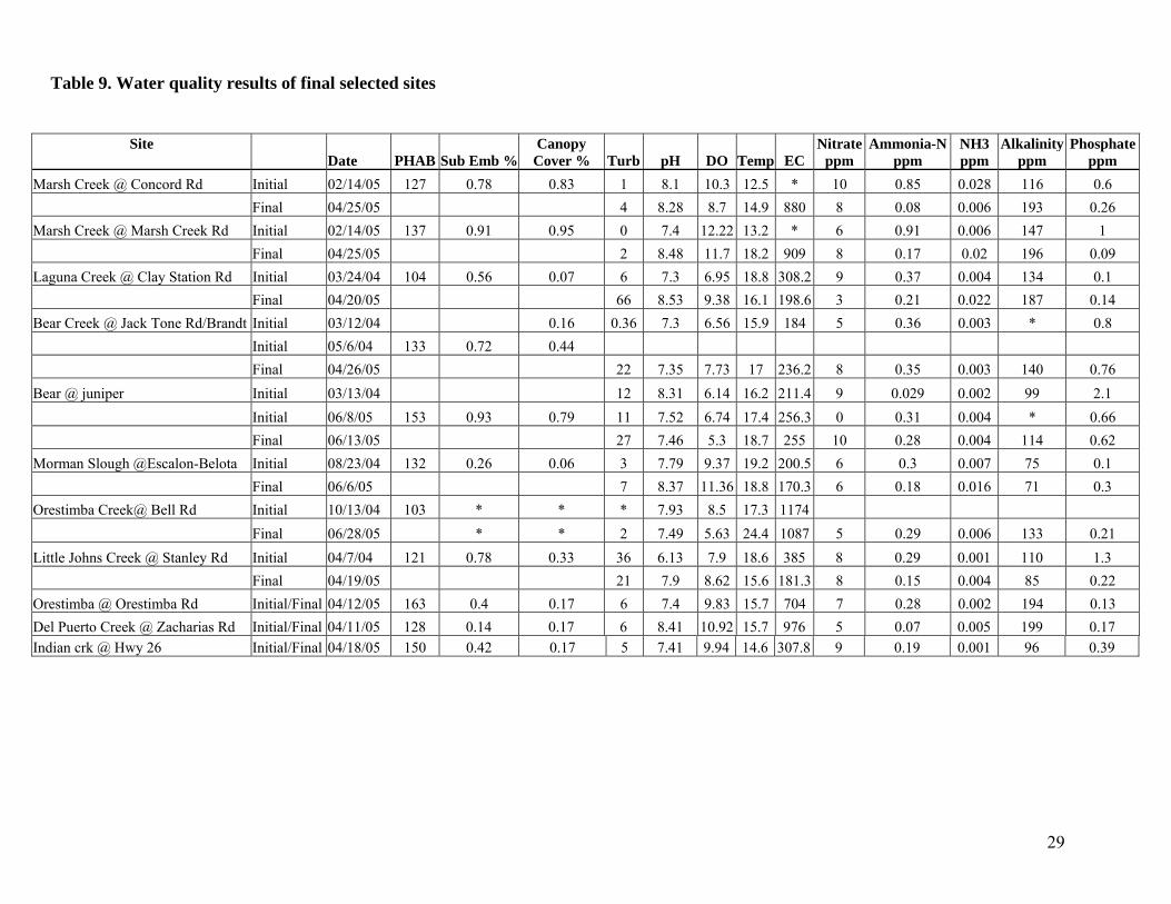
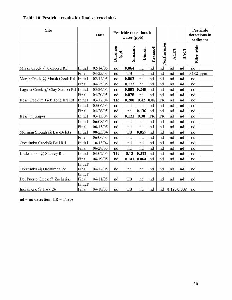
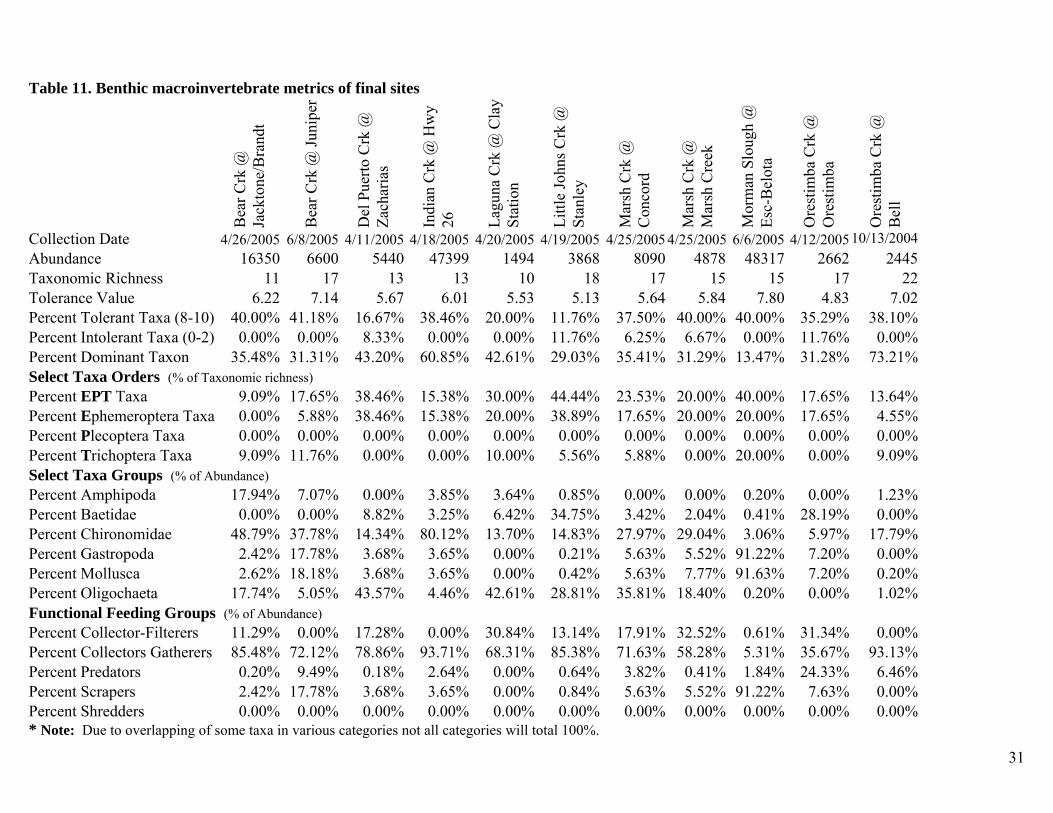
1. Pesticide Manual. 12th Ed. 2000 2. U.S.EPA. 2002. Note: ACET and DACT are simazine breakdown products. Finally, after review of all criteria, 12 of the initial 26 sites remained. The biological communities (BMIs) were then surveyed and basic water quality and pesticide analyses were repeated. Follow-up pesticide analysis revealed the pyrethroid bifenthrin in sediment at one site (13.2 ppb). The average 10-day LC50 value for Hyalella azteca is 0.52 ppb (Amweg et al., 2004). This site, therefore, was eliminated as a final reference site. These final 11 sites represent the “expected macroinvertebrate communities for “least impacted” wadable streams of the San Joaquin Valley. All physical habitat and water quality results of the final 11 sites are presented in Table 9, and pesticide results are presented in Table 10. Benthic macroinvertebrate taxa results are presented in biological metrics in Table 11.

Conclusion It is clear that the sites surveyed in the San Joaquin Valley ecoregion were heavily impacted by anthropogenic activities such as habitat modifications and runoff of pesticides, nutrients, and other pollutants. The objective was to obtain sites that were “least impacted” within a low-gradient, agricultural region of California. Ideally, a minimum of 30 sites would have been useful to provide a larger range of variability of the biotic condition of this ecoregion. To increase the number of reference sites for this region it may be necessary to gain further access to private properties. However, the final 11 sites do offer some variability under current anthropogenic conditions. These final sites represent the “least impacted” in this ecoregion, and the BMI’s from these sites represent the benchmark by which other locations within this region can be compared.

21

Periodically, these reference sites should be reassessed as mitigation measures are put into place and stream conditions change. Increased management practices, mitigation, and restoration to improve waterways in high anthropogenic, impacted areas are important objectives that will allow periodic increase of reference site benchmarks.

References

Amweg, E.L., N.M. Ureda, D.P. Weston. 2004. Use and toxicity of pyrethroids in the Central Valley. Env. Tox. And Chemistry. 24(4): 966-972. Anderson, H.B. and J.A. Buckley. 1998. Acute toxicity of ammonia to Ceriodaphnia dubia and a procedure to improve control survival. Bull. Environ. Contam. Toxicol. 61:116-122. BASIN. 2005. Boulder Area Sustainability information network. City of Boulder. U.S. Geological Survey water Quality Monitoring. [Online] http://bcn.boulder.co.us/basin/data/NUTRIENTS/info/Alk.html California Department of Fish and Game. 1998. Test 132:96-hour Acute Ceriodaphnia dubia Test for Diazinon. Aquatic Toxicology Laboratory, Elk Grove, California. CAMLnet. 2003. List of California macroinvertebrate taxa and standard taxonomic effort [Online]. Available at http://www.dfg.ca.gov/cabw/front%20page/CAMLnetSTE.pdf (verified 23 Feb. 2004) Chambers, D. and T. Messinger. 2001. Benthic invertebrate communities and their responses to selected environmental factors in the Kanawha river basin, West Virginia, Virginia, and North Carolina. NAWQA. U.S. Geological Survey. Report no. 01-4021. Cooke J, V. Connor, J. Perez, M. McGraw. 1999. Water quality management strategies: Background information and strategy design. Sacramento River Watershed Program. Regional Water Quality Control Board. Sacramento, CA. CVRWQCB, 1994. (Central Valley Regional Water Quality Control Board) Water quality control plan (Basin Plan): Central Valley Region, Sacramento River and San Joaquin River Basins. December 9, 1994. DPR. 2002. Pesticide use reporting database. Available online: http://www.cdpr.ca.gov/docs/pur/purmain.htm DPR. 2004. Bacey, J. and A. Moncada. Instructions for sampling benthic macroinvertebrates in wadable waters using the modified U.S. EPA EMAP method. California Department of Pesticide Regulation. SOP No. FSWA015.00. Available at http://www.cdpr.ca.gov/docs/empm/pubs/sops/fswa015.pdf (verified 9 March 2005)

22

Friedrich, G. D. Chapman, A. Beim. 1992. The Use of Biological Material, in D. Chapman (ed.) Water Quality Assessments, A Guide to the Use of Biota, Sediments and Water in Environmental Monitoring, (pp.171-238), Chapman and Hall, London, 238 p. Harrington, J. and M. Born. 1999. Measuring the health of California streams and rivers. Sustainable Land Stewardship Int’l. Inst. House, M.A., J.B. Ellis, E.E. Herricks, T. Hvitved-Jacobsen, J. Seager, L. Lijklema, H. Aalderink, I.T. Clifforde. 1993. Urban Drainage-Impacts on Receiving Water Quality. Wat. Sci. Tech. 27(12), 117-158. ISWP, 1991. Inland Surface Waters Plan (ISWP). Central Valley Regional Water Quality Control Board Report. Karr, J.R. and Kerans, B.L. 1991. Components of Biological Integrity: Their Definition and Use in Development of an Invertebrate IBI. U.S. EPA Report 905-R-92-003, Environmental Sciences Div., Chicago, IL, 16 p. Meng L, P.B. Moyle. 1996. Status of the splittail in the Sacramento-San Joaquin estuary. Transactions of the American Fisheries Society. 124:538-549. Moyle PB, R. Pine, L.R. Brown, C.H. Hanson, B. Herbold, K.M. Lentz, L. Meng, J.J. Smith, D.A. Sweetnam, L. Winternitz. 1996. Recovery plan for the Sacramento-San Joaquin Delta native fishes. U.S. Fish and Wildlife Service, Portland, Oregon. 193 pp. Obrebski S., J.J. Orsi, W. Kimmererer. 1992. Long-term trends in zooplankton distribution and abundance in the Sacramento-San Joaquin estuary. Interagency Ecological studies Program. Technical Report 32. May 1992. The Pesticide Manual. A World Compendium, Twelth edition. 2000. The British Crop Protection Council. Croydon, UK. Rosenberg, D.M. and V.H., Resh. 1993. Freshwater biomonitoring and benthic macroinvertebrates. Chapman and Hall. New York. Segawa, R. 1995. Chemistry laboratory quality control [Online]. Available at http://www.cdpr.ca.gov/doc/empm/pubs/sops/qaqc001.pdf (verified 23 Feb. 2004) State Water Resources Control Board. 2003. A compilation of water quality goals. [Online]. Available at http://www.swrcb.ca.gov/rwqcb5/available_documents/wq_goals/index.html#anchor274991 UF/IFAS. 2006. University of Florida, Institute of Food and Agricultural Sciences. Offices of the Cooperative Extension. [Online] Available at: http://edis.ifas.ufl.edu/BODY_FA031#FIGURE%203

23

U.S. EPA. 1986. Quality criteria for water 1986 (Gold Book): U.S. Environmental Protection Agency, Office of Water Regulations and Standards, EPA440/5-85-001. U.S. EPA 1999. Rapid Bioassessment Protocols for Use in Streams and Wadable Rivers: Periphyton, Benthic Macroinvertebrates and Fish, Second Edition. EPA 841-B-99-002. U.S. EPA; Office of Water: Washington D.C. U.S. EPA. 2001. Environmental Monitoring and Assessment Program – Surface Waters: Western pilot study field operations manual for wadable streams. Regional Ecology Branch, Western Ecology Div. April 2001. U.S. EPA. 2002. Atrazine Reregistration. Summary of Atrazine risk assessment. [Online]. Available: http://www.epa.gov/oppsrrd1/reregistration/atrazine/srrd_summary_may02.pdf U.S. EPA. 2005. Conductivity. Monitoring and assessing water quality. [Online] Available at http://www.epa.gov/volunteer/stream/vms59.html Zimmermann, E.M., R.G. Death. 2002. Effect of substrate stability and canopy cover on stream invertebrate communities. New Zealand Jrnl. of Marine and Freshwater Res. 36:537-545.

24

Habitat Assessment Field Data Sheet - Low Gradient Streams

STUDY # DATE TIME

STREAM NAME/ LOCATION

LAT LONG STREAM CLASS

FORM COMPLETED BY AGENCY

Habitat Condition Categories

parameter Optimal Suboptimal Marginal Poor 1. Epifaunal substrate/ Available Cover Greater than 50% of

substrate favorable for epifaunal colonization and fish cover; mix of snags, submerged logs, undercut banks, cobble or other stable habitat and at stage to allow full colonization potential (i.e., logs/snags that are not new fall and not transient)

30-50% mix of stable habitat; well suited for full colonization potential; adequate habitat for maintenance of populations; presence of additional substrate in the form of new fall, but not yet prepared for colonization (may rate at high end of scale)

10-30% mix of stable habitat, habitat availability less than desirable; substrate frequently disturbed or removed.

Less than 10% stable habitat; lack of habitat is obvious; substrate unstable or lacking

score 20 19 18 17 16 15 14 13 12 11 10 9 8 7 6 5 4 3 2 1 0 2. Pool Substrate characterization

Mixture of substrate materials, with gravel and firm sand prevalent; root mats and submerged vegetation common

Mixture of soft sand, mud or clay; mud may be dominant; some root mats and submerged vegetation present

All mud or clay or sand bottom; little or no root mat; no submerged vegetation

Hard-pan clay or bedrock; no root mat or vegetation

score 20 19 18 17 16 15 14 13 12 11 10 9 8 7 6 5 4 3 2 1 0 3. Pool Variability Even mix of large-shallow,

large-deep, small-shallow, small-deep pools present.

Majority of pools large-deep; very few shallow.

Shallow pools much more prevalent than deep pools.

Majority of pools small shallow or pools absent.

score 20 19 18 17 16 15 14 13 12 11 10 9 8 7 6 5 4 3 2 1 0 4. Sediment Deposition Little or no enlargement of

islands or point bars and less than <20% of the bottom affected by sediment deposition.

Some new increase in bar formation; mostly from gravel; sand or fine sediment; 20-50% of the bottom affected; slight deposition in pools.

Moderate deposition of new gravel; sand or fine sediment on old or new bars; 50-80% of the bottom affected; sediment deposits at obstructions, constrictions and bends; moderate deposition of pools prevalent.

Heavy deposits of fine materials, increased bar development; more than 80% of the bottom changing frequently; pools almost absent due to substantial sediment deposition.

score 20 19 18 17 16 15 14 13 12 11 10 9 8 7 6 5 4 3 2 1 0 5. Channel Flow Status Water reaches base of

both lower banks, and minimal amount of channel substrate is exposed.

Water fills >75% of the available channel; or <25% of the channel substrate exposed.

Water fills 25-75% of the available channel, and/of riffle substrates are mostly exposed.

Very little water in channel and mostly present as standing pools.

Par

amet

ers

to b

e ev

alua

ted

in s

ampl

ing

reac

h

score 20 19 18 17 16 15 14 13 12 11 10 9 8 7 6 5 4 3 2 1 0

Pg. 1

Figure 3. Habitat Assessment Field Data Sheet (pg 1 of 2)

25

Condition Categories

Habitat parameter Optimal Suboptimal Marginal Poor 6. Channel Alteration Channelization or dredging

absent or minimal; stream with normal pattern.

Some channelization present, usually in areas of bridge abutments; evidence of past channelization, I.e., dredging (greater than past 20 yr) may be present, but recent channelization not present.

Channelization may be extensive; embankments or shoring structures present on both banks; and 40-80% of stream reach channelized and disruptive.

Banks shored with gabion or cement; over 80% of the stream reach channelized and disrupted. Instream habitat greatly altered or removed entirely

score 20 19 18 17 16 15 14 13 12 11 10 9 8 7 6 5 4 3 2 1 0 7. Channel Sinuosity the bends in the stream

increase the streams length 3 to 4 times longer than if it was in a straight line. (Note: channel braiding is considered normal in coastal plains and other low-lying areas. This parameter is not easily rated in these areas.)

The bends in the stream increase the stream length 2 to 3 times longer than if it was in a straight line.

The bends in the stream increase the stream length 1 to 2 times longer than if it was in a straight line.

Channel straight; waterway has been channelized for a long distance.

score 20 19 18 17 16 15 14 13 12 11 10 9 8 7 6 5 4 3 2 1 0 8. Bank Stability (score each bank)

Bank stable; evidence of erosion or bank failure absent or minimal; little potential for future problems. <5% of bank affected.

Moderately stable; infrequent, small areas of erosion mostly healed over. 5-30% of bank in reach has areas of erosion.

Mostly unstable; 30-60% of bank in reach has areas of erosion; high erosion potential during floods.

Unstable; many eroded areas; "raw" areas frequent along straight sections and bends; obvious bank sloughing; 60-100% of bank has erosion scars

score (LB) Left Bank 10 9 8 7 6 5 4 3 2 1 0

score (RB) Right Bank 10 9 8 7 6 5 4 3 2 1 0 9. Vegetative Protection (score each bank) note: determine left or right side by facing downstream

More than 90% of stream bank surfaces and immediate riparian zone covered by native vegetation, including trees, understory shrubs, or nonwoody macrophytes, vegetative disruption through grazing or mowing minimal or not evident; almost all plants allowed to grow naturally.

70-90% of stream bank surfaces covered by native vegetation, but one class of plants is not well represented; disruption evident but not affecting full plant growth potential to any great extent; more than one-half of the potential plant stubble height remaining.

50-70% of stream bank surfaces covered by vegetation; disruption obvious; patches of bare soil or closely cropped vegetation common; less than one-half of the potential plant stubble remains.

less than 50% of the stream bank surfaces covered by vegetation; disruption of stream bank vegetation is very high; vegetation has been removed to 5 centimeters or less in average stubble heights.

score (LB) Left Bank 10 9 8 7 6 5 4 3 2 1 0

score (RB) Right Bank 10 9 8 7 6 5 4 3 2 1 0 10. Riparian Vegetation Zone Width (score each bank riparian zone)

Width of riparian zone >18 meters; human activities (i.e.., parking lots, roadbeds, clear-cuts, lawns or crops) have not impacted zone

width of riparian zone 12-18 meters; human activities have impacted zone only minimally.

width of riparian zone 6-12 meters; human activities have impacted zone a great deal.

width of riparian zone <6 meters; limited or no riparian vegetation due to human activity.

score (LB) Left Bank 10 9 8 7 6 5 4 3 2 1 0

Par

amet

ers

to b

e ev

alua

ted

in s

ampl

ing

reac

h

score (RB) Right Bank 10 9 8 7 6 5 4 3 2 1 0 C DPR October, 2006

Figure 3. Habitat assessment field Data Sheet (pg 2 of 2)

Pg. 2

26

Study #: __________________ Date/Time:_________________________________ Sampling Crew: ____________ Location: __________________________________ Weather Conditions: ____________________________________________________ Lat: Long: Elevation: Physical habitat quality score: Gradient: Avg. = % canopy cover: Avg. = Canopy cover = Take 4 measurements at each transect facing each direction (north, south, east & west) and average. Total reach canopy cover = the average of these 11 numbers.

Squares % Squares % Squares % Squares % 1 4 7 29 13 54 19 79 2 8 8 33 14 58 20 83 3 13 9 37 15 62 21 87 4 17 10 40 16 67 22 92 5 21 11 46 17 71 23 96 6 25 12 50 18 75 24 100

Depth: Avg. = Depth is measured in thalweg of each transect and averaged Comments:

Watershed features Description Local watershed NPS pollution Forest No evidence Field/Pasture Some potential sources Agricultural Obvious sources Residential Local watershed erosion Commercial None Industrial Moderate Other Heavy

Physical Characterization (Modified EPA multi-habitat method)

Figure 4. Physical Characterizations Data Sheet (Pg 1 of 2)

Department of Pesticide Regulation, October 2003 Side 1

27

Instream features

• Stream width is considered to be of “typical” width within approximately 5 stream widths upstream and downstream of the center of the reach.

Reach length (m) Stream width (m)

Sampling reach area (m2)

(feet x 0.3048m = meters)

Area in km2 (m2x1000) (yards x 0.9144m = meters) Aquatic vegetation (Indicate the dominant type (%) and record the dominant species present) Rooted emergent Free floating Rooted submergent Floating algae Rooted floating Attached algae Dominant species present

Portion of the reach with aquatic vegetation

Note: All water chemistry measurements, water and sediment samples are to be collected from the bottom of the reach. Diagram of reach

Physical Characterization (Modified EPA multi-habitat method)

Department of Pesticide Regulation, October 2003 Side 2

Figure 4. Physical Characterizations Data Sheet (Pg 2 of 2)

28

Study #: ______________________ Date/Time:_______________________________ Sampling Crew: _______________ Location: ________________________________ Weather Conditions: ____________________________________________________

GPS Coordinates Avg reach width Reach Length Water Quality Samples # Temperature OP –WAT EC TR – WAT DO PY – WAT PH BU – WAT Nitrate OP -SED Phosphate PY - SED Ammonia N Metals - SED Turbidity Alkalinity Water odors: (i.e. normal, fishy, sewage) Water Surface Oils: (i.e. slick, sheen, globs, flecks, none) Turbidity: (i.e. clear, slightly turbid, turbid, opaque, stained)

Diagram of reach

Water Quality Field Data Sheet (Modified EPA multi-habitat method)

Department Of Pesticide Regulation April 2005 Side 1

Figure 5. Water Quality Field Data Sheet

29

Site Date PHAB Sub Emb %

Canopy Cover % Turb pH DO Temp EC

Nitrate ppm

Ammonia-N ppm

NH3 ppm

Alkalinity ppm

Phosphate ppm

Marsh Creek @ Concord Rd Initial 02/14/05 127 0.78 0.83 1 8.1 10.3 12.5 * 10 0.85 0.028 116 0.6 Final 04/25/05 4 8.28 8.7 14.9 880 8 0.08 0.006 193 0.26 Marsh Creek @ Marsh Creek Rd Initial 02/14/05 137 0.91 0.95 0 7.4 12.22 13.2 * 6 0.91 0.006 147 1 Final 04/25/05 2 8.48 11.7 18.2 909 8 0.17 0.02 196 0.09 Laguna Creek @ Clay Station Rd Initial 03/24/04 104 0.56 0.07 6 7.3 6.95 18.8 308.2 9 0.37 0.004 134 0.1 Final 04/20/05 66 8.53 9.38 16.1 198.6 3 0.21 0.022 187 0.14 Bear Creek @ Jack Tone Rd/Brandt Initial 03/12/04 0.16 0.36 7.3 6.56 15.9 184 5 0.36 0.003 * 0.8 Initial 05/6/04 133 0.72 0.44 Final 04/26/05 22 7.35 7.73 17 236.2 8 0.35 0.003 140 0.76 Bear @ juniper Initial 03/13/04 12 8.31 6.14 16.2 211.4 9 0.029 0.002 99 2.1 Initial 06/8/05 153 0.93 0.79 11 7.52 6.74 17.4 256.3 0 0.31 0.004 * 0.66 Final 06/13/05 27 7.46 5.3 18.7 255 10 0.28 0.004 114 0.62 Morman Slough @Escalon-Belota Initial 08/23/04 132 0.26 0.06 3 7.79 9.37 19.2 200.5 6 0.3 0.007 75 0.1 Final 06/6/05 7 8.37 11.36 18.8 170.3 6 0.18 0.016 71 0.3 Orestimba Creek@ Bell Rd Initial 10/13/04 103 * * * 7.93 8.5 17.3 1174 Final 06/28/05 * * 2 7.49 5.63 24.4 1087 5 0.29 0.006 133 0.21 Little Johns Creek @ Stanley Rd Initial 04/7/04 121 0.78 0.33 36 6.13 7.9 18.6 385 8 0.29 0.001 110 1.3 Final 04/19/05 21 7.9 8.62 15.6 181.3 8 0.15 0.004 85 0.22 Orestimba @ Orestimba Rd Initial/Final 04/12/05 163 0.4 0.17 6 7.4 9.83 15.7 704 7 0.28 0.002 194 0.13 Del Puerto Creek @ Zacharias Rd Initial/Final 04/11/05 128 0.14 0.17 6 8.41 10.92 15.7 976 5 0.07 0.005 199 0.17 Indian crk @ Hwy 26 Initial/Final 04/18/05 150 0.42 0.17 5 7.41 9.94 14.6 307.8 9 0.19 0.001 96 0.39

Table 9. Water quality results of final selected sites

30

Site Date Pesticide detections in

water (ppb) Pesticide

detections in sediment

Dia

zino

n (p

pt)

Sim

azin

e

Diu

ron

Bro

mac

il

Nor

flura

zon

AC

ET

DA

CT

Bife

ntrh

in

Marsh Creek @ Concord Rd Initial 02/14/05 nd 0.064 nd nd nd nd nd nd Final 04/25/05 nd TR nd nd nd nd nd 0.132 ppm Marsh Creek @ Marsh Creek Rd Initial 02/14/05 nd 0.063 nd nd nd nd nd nd Final 04/25/05 nd 0.172 nd nd nd nd nd nd Laguna Creek @ Clay Station Rd Initial 03/24/04 nd 0.085 0.248 nd nd nd nd nd Final 04/20/05 nd 0.078 nd nd nd nd nd nd Bear Creek @ Jack Tone/Brandt Initial 03/12/04 TR 0.208 0.42 0.06 TR nd nd nd Initial 05/06/04 nd nd nd nd nd nd nd nd Final 04/26/05 nd nd 0.136 nd nd nd nd nd Bear @ juniper Initial 03/13/04 nd 0.121 0.38 TR TR nd nd nd Initial 06/08/05 nd nd nd nd nd nd nd nd Final 06/13/05 nd nd nd nd nd nd nd nd Morman Slough @ Esc-Belota Initial 08/23/04 nd TR 0.057 nd nd nd nd nd Final 06/06/05 nd nd nd nd nd nd nd nd Orestimba Creek@ Bell Rd Initial 10/13/04 nd nd nd nd nd nd nd nd Final 06/28/05 nd nd nd nd nd nd nd nd Little Johns @ Stanley Rd. Initial 04/07/04 TR 0.12 0.233 nd nd nd nd nd Final 04/19/05 nd 0.141 0.064 nd nd nd nd nd

Orestimba @ Orestimba Rd Initial/Final 04/12/05 nd nd nd nd nd nd nd nd

Del Puerto Creek @ Zacharias Initial/Final 04/11/05 nd TR nd nd nd nd nd nd

Indian crk @ Hwy 26 Initial/Final 04/18/05 nd TR nd nd nd 0.125 0.087 nd

nd = no detection, TR = Trace

Table 10. Pesticide results for final selected sites

31

Table 11. Benthic macroinvertebrate metrics of final sites

Bea

r Crk

@

Jack

tone

/Bra

ndt

Bea

r Crk

@ Ju

nipe

r

Del

Pue

rto C

rk @

Za

char

ias

Indi

an C

rk @

Hw

y 26

Lagu

na C

rk @

Cla

y St

atio

n

Littl

e Jo

hns C

rk @

St

anle

y

Mar

sh C

rk @

C

onco

rd

Mar

sh C

rk @

M

arsh

Cre

ek

Mor

man

Slo

ugh

@

Esc-

Bel

ota

Ore

stim

ba C

rk @

O

rest

imba

Ore

stim

ba C

rk @

B

ell

Collection Date 4/26/2005 6/8/2005 4/11/2005 4/18/2005 4/20/2005 4/19/2005 4/25/2005 4/25/2005 6/6/2005 4/12/2005 10/13/2004Abundance 16350 6600 5440 47399 1494 3868 8090 4878 48317 2662 2445Taxonomic Richness 11 17 13 13 10 18 17 15 15 17 22Tolerance Value 6.22 7.14 5.67 6.01 5.53 5.13 5.64 5.84 7.80 4.83 7.02Percent Tolerant Taxa (8-10) 40.00% 41.18% 16.67% 38.46% 20.00% 11.76% 37.50% 40.00% 40.00% 35.29% 38.10%Percent Intolerant Taxa (0-2) 0.00% 0.00% 8.33% 0.00% 0.00% 11.76% 6.25% 6.67% 0.00% 11.76% 0.00%Percent Dominant Taxon 35.48% 31.31% 43.20% 60.85% 42.61% 29.03% 35.41% 31.29% 13.47% 31.28% 73.21%Select Taxa Orders (% of Taxonomic richness) Percent EPT Taxa 9.09% 17.65% 38.46% 15.38% 30.00% 44.44% 23.53% 20.00% 40.00% 17.65% 13.64%Percent Ephemeroptera Taxa 0.00% 5.88% 38.46% 15.38% 20.00% 38.89% 17.65% 20.00% 20.00% 17.65% 4.55%Percent Plecoptera Taxa 0.00% 0.00% 0.00% 0.00% 0.00% 0.00% 0.00% 0.00% 0.00% 0.00% 0.00%Percent Trichoptera Taxa 9.09% 11.76% 0.00% 0.00% 10.00% 5.56% 5.88% 0.00% 20.00% 0.00% 9.09%Select Taxa Groups (% of Abundance) Percent Amphipoda 17.94% 7.07% 0.00% 3.85% 3.64% 0.85% 0.00% 0.00% 0.20% 0.00% 1.23%Percent Baetidae 0.00% 0.00% 8.82% 3.25% 6.42% 34.75% 3.42% 2.04% 0.41% 28.19% 0.00%Percent Chironomidae 48.79% 37.78% 14.34% 80.12% 13.70% 14.83% 27.97% 29.04% 3.06% 5.97% 17.79%Percent Gastropoda 2.42% 17.78% 3.68% 3.65% 0.00% 0.21% 5.63% 5.52% 91.22% 7.20% 0.00%Percent Mollusca 2.62% 18.18% 3.68% 3.65% 0.00% 0.42% 5.63% 7.77% 91.63% 7.20% 0.20%Percent Oligochaeta 17.74% 5.05% 43.57% 4.46% 42.61% 28.81% 35.81% 18.40% 0.20% 0.00% 1.02%Functional Feeding Groups (% of Abundance) Percent Collector-Filterers 11.29% 0.00% 17.28% 0.00% 30.84% 13.14% 17.91% 32.52% 0.61% 31.34% 0.00%Percent Collectors Gatherers 85.48% 72.12% 78.86% 93.71% 68.31% 85.38% 71.63% 58.28% 5.31% 35.67% 93.13%Percent Predators 0.20% 9.49% 0.18% 2.64% 0.00% 0.64% 3.82% 0.41% 1.84% 24.33% 6.46%Percent Scrapers 2.42% 17.78% 3.68% 3.65% 0.00% 0.84% 5.63% 5.52% 91.22% 7.63% 0.00%Percent Shredders 0.00% 0.00% 0.00% 0.00% 0.00% 0.00% 0.00% 0.00% 0.00% 0.00% 0.00%* Note: Due to overlapping of some taxa in various categories not all categories will total 100%.

32

Continuing Quality Control- Organophosphate Screen Water Analyses

Extraction Sample Percent Recovery

Date Numbers Ethoprop Diazinon Disulfoton Chlorpyrifos Malathion Methidathion Fenamiphos Methyl Azinphos Dichlorvos Phorate Fonophos Dimethoate Methyl

ParathionTribufos (DEF)

Profenofos

11/10/03 107,100,101, 102 105 108 108 102 107 109 116 104 82.0 84.0 90.2 87.4 95.9 93.1 80.4

3/15/05 1, 05 87.7 91.1 83.6 88.4 90.0 87.2 96.5 103 88.7 90.7 94.2 98.3 98.3 91.7 90.3

3/25/05 9, 13, 17, 21, 25, 29, (250),(253) 92.4 90.1 88.1 91.2 92.9 83.1 97.6 108 76.1 79.8 85.2 89.6 90.7 88.9 84.3

4/1/04 33, 37 94.0 93.2 80.0 89.2 93.9 93.1 84.9 90.9 78.9 78.0 85.3 86.9 87.8 94.7 87.6

7/13/04 41, 45, 49, 53** 88.2 98.0 75.9 101 76.5 74.6 78.3 63.6 84.0 86.7 88.5 90.7 93.5 98.9 86.8

8/25/04 57,(74) 84.7 94.8 74.5 100 81.8 80.5 80.2 81.2 84.6 85.9 88.2 93.1 93.4 89.6 94.4

9/15/04 61,65,69, 88.5 99.6 80.7 94.4 84.5 88.8 89.1 76.5 86.9 88.6 91.2 88.5 90.5 97.1 87.8

11/17/04 77 79.8 81.6 75.7 80.8 88.7 90.0 88.5 94.2 83.7 85.9 90.7 90.8 99.2 96.7 96.0

2/17/05 3028,3032,3036, 3040 87.7 95.2 85.8 104 87.6 94.0 91.5 76.0 73.9 75.5 79.6 82.7 84.0 83.3 83.8

4/13/05 89,93,(148),(151) 93.5 88.8 82.8 92.8 89.9 86.1 79.1 85.9 89.6 82.2 94.6 96.0 98.0 103 104

4/21/05 103,108,116,112, 120 91.7 80.0 86.6 83.6 92.8 93.2 91.6 92.9 89.5 92.4 96.1 88 97.3 97.1 96.4

4/28/05 124,128,132,136, 140 92.9 93.2 98.8 102 104 106 107 114 89.9 88.6 88.1 79.2 84.0 86.8 91.4

6/16/06 192,198,202,196 98.6 88.8 73.2 96 98 112 109 107 77.2 77.5 76.6 68 78.8 90.2 75.9

6/21/06 208 98 91.2 86.3 94.8 102 106 105 110 79.8 73.8 73.9 75.5 79.1 86.1 75.1

6/30/05 159,162 90.6 91.6 85.8 97.6 97.7 97.6 99.4 96.9 75.0 80.9 80.6 85.6 85.4 84.9 87.0

6/16/06 192,198,202,196

98.6 88.8 73.2 96 98 112 109 107 77.2 77.5 76.6 68 78.8 90.2 75.9

Average Recovery 92.0 92.1 83.7 94.6 92.8 94.6 95.2 94.4 82.3 83.0 86.2 85.5 89.7 92.0 87.3

Standard Deviation 6.1 6.6 9.4 6.7 8.2 11.5 11.7 14.5 5.6 5.7 6.9 8.9 7.3 5.5 8.1

CV 6.68 7.19 11.19 7.09 8.82 12.21 12.31 15.39 6.78 6.84 8.03 10.39 8.12 6.03 9.31 Upper Control Limit 123 117 119 119 126 128 125 137 106 110 113 117 119 126 125 Upper Warning Limit 113 109 109 111 116 117 115 122 98 102 105 108 111 116 115 Lower Warning Limit 70.7 77.2 68.1 77.2 75.7 74.6 77.3 64.0 67.0 73.5 75.5 73.2 76.6 74.9 74.2 Lower Control Limit 60.2 69.2 58.0 68.8 65.7 63.9 67.9 49.4 59.2 66.3 68.1 64.5 68.0 64.7 64.1

* Highlighted cells are percent recoveries exceeding control limits **Began using GC/MS for diazinon and chlorpyrifos, RL dropped to 10ppt. Sample numbers in ( ) are blind spikes.

Appendix I: Continuing Quality Control and Blind Spike Analyses

33

Continuing Quality Control- Triazine Screen Water Analyses

Extraction Sample Percent Recovery

Date Numbers Spike Atrazine Simazine Diuron Prometon Bromacil Prometryn Hexazinone Metribuzin Norflurazaon DEA (Deethyl)

ACET (Deiso) DACT Propazine

(Surrogate)

1 93.5 98.0 99.5 93.5 105 90.0 93.0 94.5 98.5 95.5 94.5 93.0 88.03/25/2004 2, 7, 10, 14, 18, 22, 26, 30, 251, 240 2 85.5 88.0 92.0 89.0 100 87.0 87.0 88.5 96.0 92.0 86.5 90.5 81.5

1 91.0 90.5 95.5 92.0 102 88.5 89.0 97.5 97.5 93.0 89.5 93.5 89.04/2/2004 34, 38 2 88.5 87.0 103.0 90.5 102 88.0 90.5 85.0 100 90.5 92.5 99.5 89.51 74.0 76.5 81.5 78.5 79.5 73.5 69.0 77.5 89.5 78.0 76.5 76.0 78.07/16/2004 42, 46, 50, 54 2 81.0 83.5 90.0 87.5 91.0 83.5 74.0 108 96.0 88.0 77.5 86.0 83.01

89.0 92.5 90.0 91.5 96.0 93.0 99.0 86.0 106 98.0 82.5 99.0 90.59/1/2004 58, (75)

2 97.5 99.0 108.0 97.5 99.5 104 104 98.5 112 109 92.5 100.0 98.01 90.0 90.5 93.0 92.5 103.0 95.0 112 100 112 84.5 88.5 94.0 90.59/16/2004 62,66, 70

2 91.5 86.0 101 89.0 97.0 90.5 107 92.5 110 87.5 82.5 92.5 88.51 86.0 101 112 105 112 105 110 103 108 112 84.5 93.5 11411/29/2004 78

2 93.0 98.5 116 105 103 97.0 119 109 101 104 84.5 87.0 87.51 89.5 89.5 90.5 91.0 94.0 92.5 106 90.0 96.5 93.0 94.5 87.5 90.52/25/2005 82, 86

2 89.5 89.0 89.5 92.5 97.0 92.0 104 95.5 97.5 92.0 90.0 80.5 93.51 86.0 93.0 91.5 86.0 88.0 87.0 88.5 80.5 98.0 88.5 82.0 89.0 83.54/29/2005 90,(149),94,104,109,117,1

13,121,125, 129,133 2 77.0 78.0 85.5 75.0 78.5 76.0 86.0 69.0 90.0 82.0 72.0 79.0 74.5

1 78.5 82.0 81.5 86.0 87.5 77.5 94.0 78.0 90.0 85.0 86.5 79.0 76.56/28/2005 137,141

2 83.0 88.0 92.0 91.5 97.5 81.5 108 74.5 101 93.5 90.5 84.5 78.56/26/2006 193,199,203,197,211 1 83.5 88.5 87.0 91.0 97.5 90.5 92.0 85.0 97.0 63.5 81.0

Average Recovery 86.7 89.4 94.7 90.8 96.3 89 96.3 90.4 99.6 92.2 86.6 87.8 87.2

Standard Deviation 6.06 6.7 9.6 7.18 8.44 8.60 13.02 11.51 7.16 8.78 6.68 9.21 9.00

CV 6.99 7.5 10.2 7.91 8.77 9.67 13.52 12.73 7.19 9.52 7.72 10.49 10.32

Upper Control Limit 105 108 118 106 117 111 121 110 113 116 140 101 115

Upper Warning Limit 98.2 101 109 99.2 111 105 113 103 107 109 128 95.7 107

Lower Warning Limit 72.2 73.2 73.4 73.8 84.9 78.9 76.9 75.0 84.8 79.1 78.3 73.7 72.4

Lower Control Limit 65.8 66.3 64.4 67.4 78.4 72.4 68.1 68.0 79.2 71.7 66.0 68.2 63.8*Highlighted cells are percent recoveries exceeding control limits, Sample numbers in () are blind spikes.

34

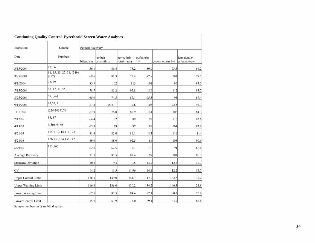
Continuing Quality Control- Pyrethroid Screen Water Analyses

Extraction Sample Percent Recovery

Date Numbers bifenthrin

lambda cyhalothrin

permethrin (cis&trans)

cyfluthrin 1-4 cypermethrin 1-4

fenvalerate/ esfenvalerate

3/15/2004 03, 06 56.1 86.4 78.2 80.0 73.3 66.2

3/25/2004 11, 15, 23, 27, 31, (249), (252) 69.6 81.3 77.4 97.8 101 77.7

4/1/2004 35, 39 85.5 102 113 101 95 93.2

7/15/2004 43, 47, 51, 55 78.7 85.2 97.8 119 112 95.7

8/25/2004 59, (76) 65.0 74.5 87.1 95.5 93 87.4

9/15/2004 63,67, 71 67.4 75.5 77.6 103 92.5 92.3

11/17/04 (224-1037),79 67.9 78.8 82.9 114 106 84.3

2/17/05 83, 87 64.4 82 89 92 116 83.6

4/13/05 (150), 91,95 65.3 79 87 89 104 82.0

4/21/05 105,110,118,114,122 81.4 82.0 89.1 113 116 114

4/28/05 126,130,134,138,142 89.0 88.0 92.5 86 108 90.6

6/29/05 163,160 62.8 62.5 77.1 76 94 68.6

Average Recovery 71.1 81.5 87.4 97 101 86.3

Standard Deviation 10.1 9.3 10.5 13.7 12.3 12.7

CV 14.2 11.5 11.96 14.1 12.2 14.7

Upper Control Limit 128.9 149.0 141.7 147.2 162.8 137.2

Upper Warning Limit 116.6 136.0 130.2 134.2 146.3 124.8

Lower Warning Limit 67.5 81.5 84.4 82.1 80.2 75.0

Lower Control Limit 55.2 67.9 73.0 69.1 63.7 62.6

Sample numbers in () are blind spikes.

35

Extraction Sample Percent Recovery Date Numbers bifenthrin fenopropathrin

lambda cyhalothrin epimer

lambda cyhalothrin permethrin cis permethrin trans cyfluthrin cypermethrin

fenvalerate/ esfenvalerate delta methrin resmethrin

6/15/2006 194,200,204,213 81.3 110 95.3 95.0 87.7 96.0 100 100 97.3 82.3 74.3

6/20/2006 212 89.7 116 103 104 98.7 104 104 107 103 91.3 89.3

7/26/2006 2250, 2229, 2232, 2235 64.2 55.0 74.0 77.6 74.8 70.6 83.4 80.6 65.6 53.2 80.4

7/19/2006 269 62.9 67.1 71.5 75.0 68.8 68.5 77.6 78.3 64.3 55.3 71.6

6/30/2006 226, 271, 272, 270 67.0 68.1 69.7 71.9 83.5 74.5 75.7 80.9 65.2 54.2 73.6

Average Recovery 73.0 83.2 82.7 84.7 82.7 82.7 88.1 89.4 79.1 67.3 77.8

Standard Deviation 11.9 27.7 15.3 14.0 11.6 16.2 13.0 13.2 19.3 18.1 7.2

CV 16.3 33.3 18.5 16.6 14.0 19.5 14.8 14.8 24.5 27.0 9.25

Upper Control Limit 98.6 97.3 99.8 99.2 98.9 101 110 93.0 99.0 104 88.9

Upper Warning Limit 91.8 89.1 92.8 92.4 92.0 92.4 100.4 86.0 91.4 93.9 81.4

Lower Warning Limit 64.5 56.3 64.8 64.8 64.3 56.4 61.1 56.9 61.5 53.5 51.4

Lower Control Limit 57.6 48.1 57.9 58.0 57.4 47.4 51.3 49.6 54.0 43.4 43.8 *Highlighted cells are percent recoveries exceeding control limits

36

Blind Spike Data

Extraction Date Sample

Number Screen Pesticide Spike Level Recovery Percent

Recovery Exceed CLb

3/25/04 251 TR Norflurazon 0.35 0.373 107 UWL

3/25/04 240 TR Simazine 0.5 0.454 90.8 No

Diuron 0.75 0.727 96.9 No

3/25/04 250 OP Malathion 0.20 0.167 83.5 No

Dimethoate 0.35 0.323 92.3 No

3/25/04 253 OP Chlorpyrifos 0.25 0.227 90.8 No

3/25/04 249 PY Bifenthrin 100 76 76.0 No

Cypermethrin 120 118 98.3 No

3/25/04 252 PY L. Cyhalothrin 50 44.5 89.0 No

8/25/04 76 PY Bifenthrin 40 40.1 100 No

Permethrin 200 214 107 No

8/25/04 74 OP Diazinon 0.15 0.135 90.0 No

Dimethoate 0.25 0.207 82.8 No

9/1/04 75 TR Atrazine 0.30 0.252 84.0 No

Norflurazon 0.15 0.148 98.7 No

11/17/04 224-1037 PY Cyfluthrin 250 284 114 No

Esfenvalerate 200 194 97.0 No

11/17/04 224-1036 OP Chlorpyrifos 0.03 0.0244 81.3 No

Methidation 0.15 0.158 105 No

4/13/05 148 OP Methylparathion 0.20 0.205 103 No

4/13/05 151 OP Diazinon 0.15 0.141 94.0 No

4/13/05 150 PY Permethrin 0.35 0.262 74.9 LWL

4/29/05 149 TR Simazine 0.25 0.22 88.0 No b CL=Control Limit; Upper CL (UCL), Lower CL (LCL).