Bank of Israel

Research Department

The Determination of Real Wages in the Long Run and its Changes in the Short Run –Evidence from Israel: 1968-1998

1 by

Yaacov Lavi* and Nathan Sussman** Discussion Paper No. 2001.04

February 2001

________________________ * Research Department, the Bank of Israel. ** Department of Economics, Hebrew University. 1 We thank Igor Frenklakh, Karine Gabay and especially Adi Tropp for their research

assistance. We would like to thank Yael Artstein and Zvi Hercowitz for their comments and for those of participants in the research department of the Bank of Israel seminar and the Israeli economic Association annual conference.

Any views expressed in the Discussion Paper Series are those of the

authors and do not necessarily reflect those of the Bank of Israel. 91007 ירושלי. 780ד "בנק ישראל ת, מחלקת המחקר

Research Department, Bank of Israel, POB 780, 91007 Jerusalem, Israel WWW.BANKISRAEL.GOV.IL

Abstract

In this paper we study the determination of real wages in Israel for the long and short run during 1968-98. This period serves as a uniquely rich macro-economic laboratory as the Israeli economy went from hyper-inflation to low inflation, liberalization of the economy, decline of the powerful national trade union, massive immigration, influx of foreign workers and finally a high-tech led economic growth. We employ a simple Neo-Classical framework in which long run real wages are determined according to labor productivity. This allows for a clear dichotomy between the long run and short-run. The long run is estimated using co-integration techniques whereas the short-run real-wage dynamic equations are linked to the long-run relationship via an error-correction term. The results of our study relate to important debates in the macroeconomic analysis of labor markets: Despite many competing theories based on market imperfections and complex institutions, we provide empirical support to the Blanchard and Katz (1997) approach and can not refute the simple neo-classical framework and find that in the long-run real wages are co-integrated with unit elasticity with labor productivity. In the short run we find, on the one hand, rising importance of market forces and evidence of nominal contracting with rational expectations such that real wages are affected only by unexpected inflation. On the other hand, unemployment benefits have increasingly produced real wages rigidities. These rigidities may in fact outweigh the short-term effect of the decline of the Histadrut- the national trade union.

2

1. Introduction

The study of real wage determination in the long and short-run offers many insights into

important issues related to macroeconomic stability and growth. Macroeconomic stability

is affected by forces that cause real wages to deviate from market clearing equilibrium –

are they of short or prolonged nature? Are they related to real or nominal shocks? Are they

the outcome of trade union or government intervention, monetary or fiscal policies?

Economic growth is affected by the efficiency with which the labor market allocates

resources. Are real wages determined in a way that rewards productivity? In this paper we

attempt to shed light on some of these issues by estimating, using quarterly data, both long-

run and short-run real wage equations for the Israeli economy for the period 1968-1998.1

The Israeli economy went through many changes during the period we study; the economy

moved from high inflation and wage indexation to a low inflation rate with little

indexation. It saw a shift from the dominance of a national trade-union to the rising

importance of individual labor contracts. The economy went from specialization in

traditional occupations to become a leading high-tech economy. The period saw a rising

degree of political intervention in labor-market legislation related to unemployment

benefits and minimum wages. On the other hand, the economy was opened to foreign labor

both after the six days war (1967) and again in the 1990s. Moreover, the Israeli labor

market was subject to the experience of a large inflow of immigration. These dramatic

1 The short-run equations were estimated for period 1971-1998 due to the lags in some of the independent variables.

3

changes make the Israeli labor market a very rich economic laboratory that abounds with

exogenous changes. Such an economic environment allows us to put to the test the

hypothesis that in the long-run the labor-market operates along neo-classical lines where

wages are ultimately determined according to labor productivity and that institutional

change and macro-economic instability affects mainly the short-run dynamics of the labor

market. It also allows us to estimate the length of time it takes for labor markets to return

to the long run equilibrium. We therefore reconcile the numerous theories advanced to

address labor market rigidities with the neo-classical model. The former are better suited to

the analysis of labor-market dynamics, while the later is a useful in characterizing long-run

equilibrium.

We utilize a simple neo-classical labor market model, in the spirit of Blanchard and Katz

(1997) to address the issues of long-run wage determination and the short-run dynamics of

the labor market. The neo-classical approach posits that in the long-run wages should equal

the marginal product of labor. This approach provides a clear dichotomy between the long

and short run that goes hand in hand with contemporary time-series econometric

techniques: For the long run we need only to obtain cointegration between real wages and

productivity, whereas the short run is estimated as a dynamic process linked to the long run

via the error-correction term of the long run cointegrating relationship. In the short-run,

real wages may deviate from their long-run equilibrium due to a variety of causes that may

be consistent with other models such as efficiency wages as in Jullien and Picard (1998),

4

bargaining (Calmfors, 1990) and search models and may be the outcome of various

rigidities and market imperfections.

We demonstrate, following the specification by Sachs (1979), that in the long-run, over the

last 30 year period stretching from 1968 to 1998, the real wage is cointegrated with labor

productivity with unit elasticity. This result is consistent with the neo-classical competitive

wage model with a constant returns-to-scale Cobb-Douglas production function and a

stationary labor share of income.2 We also directly estimated an unrestricted production

function and obtained a good fit with our underlying assumption. While this result is also

consistent with a situation whereby the Histadrut – the powerful national trade union - sets

wages and employers set employment in such a way that labor productivity adapts to real

wages, it unlikely that in such a situation the economy will arrive at long-run full

employment. The Israeli experience that exhibited low unemployment levels, relative to

Europe, does not appear to support this interpretation. On the other hand, wage bargaining

at the national level may take into account developments in labor productivity in order to

maintain full employment in the long run. For the period of a strong trade union, our

findings are consistent with the latter interpretation. For more recent years it possible that

trade unions have some market power in the short run but in the long run wages are

determined according to labor demand.

2 This result could also be consistent with a model in which real wages are sticky and unemployment is stationary. However, it is not so easy to motivate such a result in which the sticky real wages is cointegrated with labor productivity.

5

We then proceed to investigate the short-run dynamics of real wages in an attempt to

explain its short-run deviations from its, stationary, long-run trend. Figure 1 shows these

deviations. One surprising result is that the period of rapid and accelerating inflation, from

1977 to 1985, was one in which deviations from the long-run equilibrium were the smallest

and the shortest. In contrast, the period of disinflation is marked by long swings of

deviations from the long-run equilibrium: A relatively long adjustment cycle from 1986 to

1990 followed by a continuing deviation from trend ever since 1991. These phenomena

pose a challenge since it is common knowledge that during recent years the labor market

became more competitive with the breakdown of the Histadrut and the privatization of

many large companies.

Our short-run analysis may account for this apparent paradox. We are able to show that

while, indeed, market forces play a more significant role, reflected by the significance of

productivity in the short-run equations following the stabilization program, they have

directly and indirectly introduced rigidities and noise into the labor market. In the

inflationary period, wage contracts were supplemented by a cost-of-living (indexation)

allowance. Therefore, nominal shocks and surprises had a smaller relative effect on real

wages than observed today, when the practical dissolution of these allowances exposed the

labor market to the effect of unexpected nominal shocks. The prolonged disniflation, its

magnitude largely unexpected by the public may have caused real wages to diverge from

their long-run equilibrium. Thus, though inflation may have acted to slow down

productivity growth in the long-run, in terms of short-run labor market dynamics,

6

disinflation was more costly. Contrary to Keane (1993) we find that with the shift from

wage setting that included institutional wage indexation to market based wage setting, we

can not refute the hypothesis that agents engage in nominal wage contracting with rational

expectations that employs expectations consistent with those derived from the capital

market.

The breakdown of the Histadrut and privatization of government and histadrut owned

conglomerates led to the growing recourse to unemployment benefits that protect labor

from the vagaries of the now more competitive labor market. Those had the effect, as has

been recorded in numerous studies, to exacerbate the rigidities in the labor market that

seemed not to be as severe during the period of central wage negotiations conducted by the

government and the Histadrut. It seems that their presence lowered the significance of

unemployment as an incentive to bring down real-wages to their long-run equilibrium

rates. As Tor, Verdin and Warne (1998) and Bender and Thesdossiou (1998) recently

showed there is little significance in the relationship of real-wages and unemployment.

Thus, the prevalence of unemployment benefits at a time when the labor market was

subject to disinflation surprises that increased unemployment may have acted to lock-in

those, otherwise, temporary deviations of real wages from their long run levels.

The paper is organized in the following way. In section 2 we outline our methodological

approach. In section 3 we provide a short description of the evolution of the major labor

market variables and carry out our empirical investigation. Section 4 concludes.

7

2. Methodology: Determination of wages in the labor market.

A. The Long Run

Our approach addresses two issues: the determination of wages in the long run and the

short run dynamics of the labor market. We employ the basic neo-classical labor market

framework, following Blanchard and Katz (1997) and posit that real wages are set to equal

the marginal product of labor (labor productivity). According to this approach the labor

demand curve in the long run is perfectly elastic with respect to the quantity of labor

employed.3 There are a number of theories that explain the determination of real wages; In

the efficiency wages model, real wages are offered by the firm to boost effort

(productivity) whereas in wage bargaining models insiders bargain for higher real wages at

the expense of outsiders. 4 However, our approach is that in the long-run, when producers

can adjust all factors of production and markets are allowed sufficient time to adjust, the

neo-classical competitive model should hold. Having established that (in the empirical

section), we can focus on the short-run dynamics that offer the interesting insights on the

adjustment of the labor market to the various macro-economic and institutional changes.

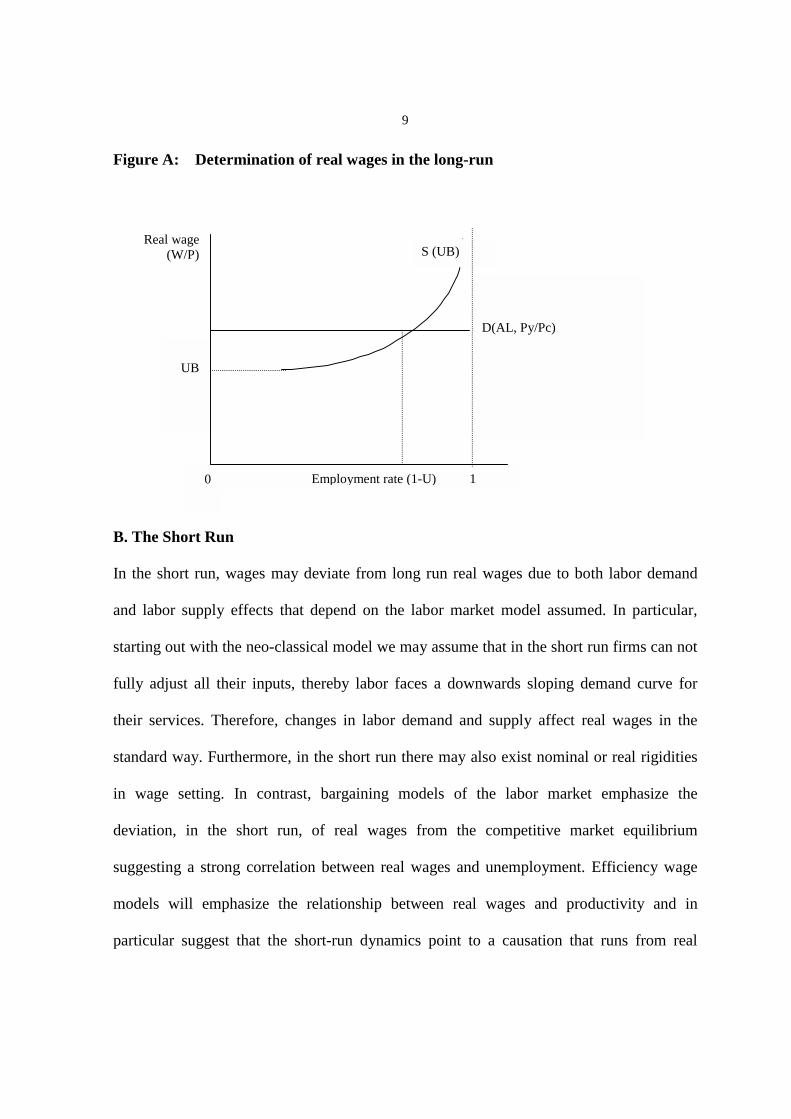
To conclude, our key assumption is that in the long-run the demand curve for labor is

independent of the level of employment rate (see figure A). The important implication of

this assumption is that in the long-run real wages are determined by demand factors alone.

Real wages, therefore, may be represented as a function of labor productivity (AL) and the

relative price of producer to consumer goods (Py/Pc) (an adjustment made to correct real

3 In the empirical section we also test the hypothesis that the demand curve is downwards sloping in the long-run. 4 Three theories summarized in Blanchard and Katz (1997) are the basic neo classical theory, efficiency wage theory and job search theories.

8

wages in producer prices to the measured real wages in consumer prices, allowing us to

jointly present both the demand and supply sides of real wages). We assume a CES

aggregate production function and specify the following real wage function:

(1) )()( 21 PcPylyw −+−= ββ

Where w is the log of the real wage, y is log output, l – is log of the employment and Py

and Pc are the log of the producer and consumer price levels 5. In the general case,

β1=1/σ - the inverse of the elasticity of substitution between capital and labor, and β2

should equal 1. In the special case of a Cobb-Douglas function β1 and β2 should each equal

1. If β1,is equal to 1, this formulation is equivalent to the hypothesis that in the long run

the labor share of output is constant.6 Therefore, one can conduct the empirical analysis in

two parallel channels: short run wage equations and the analysis of the short run deviations

of the labor share of output from its equilibrium (constant) level.

There also exist the usual upwards sloping long-run labor supply curve in which the share

of the labor force willing to work is a function of the real wage and the reservation wage

(UB unemployment benefits).7 Alternatively, this curve can be specified as an effort curve

(according to efficiency wages model) or a bargaining curve according to bargaining models.

The intersection of the two curves determines the long run equilibrium employment rate

(=1-U*, U* - the natural unemployment rate).

5 This specification is identical to the one used by Sachs (1979), p. 251. 6 In the empirical section we report our findings that can not reject our assumption regarding a Cobb-Douglas production function.. 7 We differentiate between those included in the labor force, to collect unemployment benefits, and those actually wishing to work.

9

Figure A: Determination of real wages in the long-run

B. The Short Run

In the short run, wages

and labor supply effec

starting out with the neo

fully adjust all their in

their services. Therefor

standard way. Furtherm

in wage setting. In c

deviation, in the shor

suggesting a strong cor

models will emphasiz

particular suggest that

UB

S (UB)

D(AL, Py/Pc)

wage W/P)

0

Employment rate (1-U) 1

Real(

may deviate from long run real wages due to both labor demand

ts that depend on the labor market model assumed. In particular,

-classical model we may assume that in the short run firms can not

puts, thereby labor faces a downwards sloping demand curve for

e, changes in labor demand and supply affect real wages in the

ore, in the short run there may also exist nominal or real rigidities

ontrast, bargaining models of the labor market emphasize the

t run, of real wages from the competitive market equilibrium

relation between real wages and unemployment. Efficiency wage

e the relationship between real wages and productivity and in

the short-run dynamics point to a causation that runs from real

10

wages to productivity. Another approach is to divide the labor market into two segments:

high and low skill. According to this approach, in the short run the supply of workers

endowed with the new high-tech skills is limited and thereby real wages may deviate much

more, and employment deviate much less, with changes in demand.8 Conversely, the

supply of low skill workers is very elastic and therefore we will observe smaller deviations

of the real wage from its long run levels.

Government intervention may also affect the short-run real wage. The two common sorts

of intervention are the setting of minimum wages and the allocation of unemployment

benefits. Assuming that minimum wages are binding, whenever they are increased they

increase the average real wage in the economy. Their existence, introduces a lower bound

on labor demand curve and causes wages to deviate in the short run from their long-run

equilibrium rate. However, these effects are limited to the short-run. In the long-run firms

will adjust their other inputs such that the minimum wage will be equal to labor

productivity. Unemployment benefits act to increase the reservation wage of workers

thereby lowering labor supply. In the bargaining model they reduce the cost of militant

action on the part of unions and in efficiency wages model they reduce the cost of shirking

(being fired) thereby increasing the cost of wage contracts. Therefore, the effect of

unemployment benefits is equivalent to a reduction in labor supply that raises the real

wage.

8 However, the changes in productivity in the high tech sector will, in the long run, affect labor productivity and wages throughout the economy.

11

In practice since wages are set in nominal terms, aimed at achieving the market clearing

real wage, it is possible that the ex-post measured real wage may deviate from the ex-ante

expected real wage.9 The difference between the ex-ante and ex-post real wage may arise

due wrong expectations on the inflation rate, nominal rigidities and inflation surprises.

Therefore, an important issue in analyzing the short run dynamics of real wages (and

unemployment) is the structure of inflation expectations. Whatever may be the source of

deviation of ex-post real wages from the long run equilibrium level, the neo-classical

approach we adopt assumes that there are market forces that act to restore the long term

equilibrium real wage rate.

Following our preferred, neo-classical, approach, we can specify similarly to Layard,

Nickel and Jackman (1991), assuming rational expectations, the short run ex-ante real

wages dynamics in the following way:

( )

)( )5(

)4(

)3()()( )2( 11111

ettt

at

tat

ettt

ttttttSt

Dtt

wwWwwW

lyPcPywXXaw

ππππ

ελδβ

−−∆=∆

−∆=∆

+∆=∆

+−−−−−++=∆ −−−−−

Where w is the ex-ante real wage, W is the nominal wage contract and wa is the actual (ex-

post) real wage; a is a constant XD and Xs are, respectively, demand and supply effects. The

term in parentheses is the error-correction term which corrects for previous period’s

deviation from the equilibrium real wage (as specified in equation (1)), π is actual inflation

9 This is especially true for recent experience in the Israeli labor market whereby the cost of living allowance is not effective in low inflation environment.

12

and πe is the expectations at time t of inflation expected at t+1 , ε is a random shock to real

wages. The equation for estimation is:

(6) ( ) ( ) ttttttSt

Dt

ett

at lyPcPywXXaw ελδβππ +−−−−−++−−=∆ −−−−− )()( 11111

According to this specification ex-post real wages are affected by deviation of actual

inflation from expected inflation. The assumption of rational expectations, reflected in a

unitary elasticity of unexpected inflation with respect to ex-post real wages, allows us to

de-couple the (real) labor market variables affecting real wages and the effect of nominal

surprises.

3. Empirical results 3.I The long-run. As discussed in the methodological section, in the long run, the labor demand curve is

derived from a CES type production function. In this section we assume that the

production function is a constant returns to scale Cobb-Douglas production function. Thus,

real wages (in producer prices) are determined according to labor productivity and

employment, which doesn’t affect the real wage, is determined by labor supply.

We proceeded to estimate the following long-run real wage equation:

(7) εββα +++=PcPy

LYw loglog)log( 21

13

Where w is the average wage per worker in the business sector divided by the consumer

price index.

Labor productivity (Y/L) is real output (in the business sector) per worker.

Producer prices are the implicit GDP deflator. Since the series are unit root we employed

the Engle-Granger method to test for long-run cointegration.

The results, reported in Table 1 support the neo classical model of the long-run

determinants of real wages.10 We find an elasticity of 1 between changes in real wages and

changes in labor productivity, which is consistent with a Cobb-Douglas production

function with constant returns to scale.11 A Cobb-Douglas constant-returns-to-scale

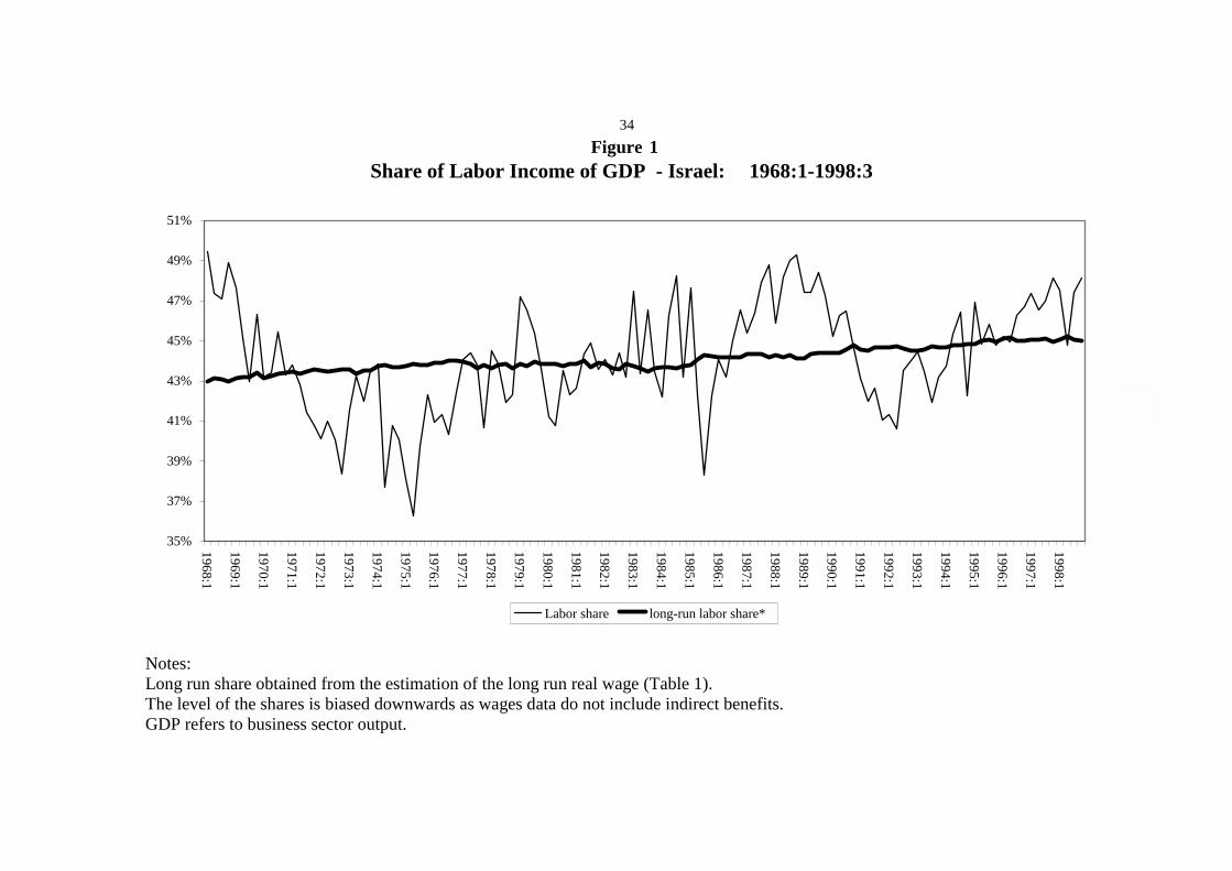
production function implies constant labor and capital income shares out of output. Figure

1, based on annual averages, demonstrates that indeed labor shares were fairly constant

throughout the sample period.12 Further evidence is provided by unit root tests that show

that the labor share of output is stationary throughout the entire period we investigate.

10 The cointegration test reports that the series are cointegrated, however cointegration does not imply causality and therefore at this point we do not wish to rule out models such as efficiency wage models which assume a reverse causality between wages and productivity. 11 We conducted tests, regarding the validity of our assumption about the aggregate production function. The results, reported in Table A1 suggest we can not reject the assumption of a Cobb-Douglas formulation and is consistent with our finding of an elasticity of 1 in the long-run regression. An unrestricted estimation yielded a labor share of 0.65 and a capital share of 0.35. We also estimated an unrestricted CES production function from which we can compute an elasticity of substitution of 0.6 which is inconsistent with the Cobb-Douglas specification. 12 Our measure is based on the sum of wages reported by National Security sources and the return to labor of self-employed. This calculation excludes employers’ contributions and benefits that are not included in wages. However, this omission affects only the level of the labor share of income and not its trend. To verify that our definition of income does not affect the results we also estimated equation 1 using annual National Accounts data that include all non-wage benefits. The results, are reported in Table A4, show that the elasticity of substitution between labor and capital ranges from 0.85 to 1.05 which is closer to our estimation of .95 than the CES specification with an elasticity of substitution of 0.6.

14

While we can not reject our assumption about the nature of perfect elasticity of the long-

run demand curve for labor, we wanted to test the competing hypothesis of a downwards

sloping demand curve for labor. Under our hypothesis of a perfectly elastic labor demand

schedule we can fully identify (econometrically) the demand curve by demand factors

alone. Under the alternative hypothesis of a downwards sloping demand curve we need to

include supply (shift) factors in order to identify the demand curve. We included the

reservation wage (unemployment benefits) which are also unit root and estimated a

Johansen and an Engle-Granger cointegration equation. The results are reported in Table

A2. While we could obtain cointegration the results were less significant (rejection of no

cointegration at the 5% level compared to 1% and a lower adjusted r-square in the

regressions) than those derived under the perfectly elastic demand curve assumption.

Therefore, while we can not reject either hypothesis about the nature of the long run

demand curve for labor, econometric evidence tends to favor the perfectly elastic demand

curve specification. Furthermore, we prefer the simpler and more convenient specification

rather than the more (unnecessarily) complicated one.

The adjustment factor introduced to account for the difference between producer and

consumer prices is also significant, and close to unity. Recall from the methodology

section that we require the coefficient to be equal to 1 in order to be able to conduct the

transformation between real wages measured in producer prices (that equal the marginal

product of labor) to the estimated real wage, measured in consumer prices. Attempts to

15

include indirect taxes in the equation to account for the difference between factor prices

and market prices did not produce significant results.

Our findings suggest that in the long-run, defined as the 30 year included in our sample,

the Israeli labor market did not suffer from long-term rigidities - real wages did not

permanently deviate from those predicted by neo-classical economic theory.13 This, despite

the presence of a large government sector, a strong trade union (the Histadrut) and the big

changes in the economic environment – the oil crisis, rapid inflation, stabilization and mass

immigration. Nevertheless, as can be gleaned from figure 1 the deviations from long-run

equilibrium may be quite long. At the same time, unemployment (figure 3a) has risen in

the late 1980s and 1900s. However, the finding of no long term rigidities in real wages

suggests that the rise in unemployment can be defined as a rise in natural unemployment.

This rise could be due to the institution of unemployment benefits and minimum wages or

perhaps hysterisis - whereby unemployment due to short run deviations from equilibrium

in the labor market get locked in for the long run. Oddly enough, the period of rapid

inflation is characterized by a relatively faster adjustment to long-run equilibrium, perhaps

due to the presence of an effective cost of living adjustment mechanism. We return to this

point bellow.

13 Artstein (1997), arrived to a similar conclusion in her dissertation.

16

3.II The short-run.

According to the model presented above, the short-run dynamics of the real wage are more

complex than those of the long-run. In the short run, the labor demand curve is downwards

sloping and therefore real wages are determined not only by labor demand but also by

labor supply. Recall that under the perfectly-elastic demand curve result we obtained

above, demand determines real wages while labor supply determines employment. In the

short-run real wages are determined by both labor demand and supply. Following equation

(6) from the methodology section, we classify these deviations into 4 explicit categories:

demand factors XD, supply factors XS, lagged labor market effects (lagged values of

unemployment) and nominal rigidities (the effect of unexpected inflation). Remaining,

unobservable, labor market rigidities are captured by the error-correction term that we

derive from the long-run estimation. When the error correction terms is significant, and has

the correct sign, this method ensures the convergence of wages to their long-run

equilibrium.14 We estimated regressions, using quarterly data, that cover the whole sample

– from 1971 to 1998 and because the 1985 stabilization is considered a watershed in the

Israeli economy we also estimated regression that cover the pre and post stabilization

periods.15 Results of our estimation are reported in Table 1. We also estimated the

equations for the 1990s, partly as a sensitivity test and mainly because we were interested

to test whether recent events tell a different story. The 1990s abound with important labor

14 The error term of the long-run co-integration equation. 15 The 1985 stabilization reduced annual inflation rates from 400% to 20%. More importantly there was a fiscal and monetary regime shift with the adoption of deficit reduction policies and the termination of the accommodation of monetary policy to the financing of the deficit.

17

market developments – the decline in the power of the Histadrut, mass immigration from

the former Soviet Union, influx of foreign workers from Asia and Eastern Europe, the

opening up of the economy, privatization and disinflation. As shown bellow, the results for

the 1990s suggest a significant change in the specification of the regression suggesting that

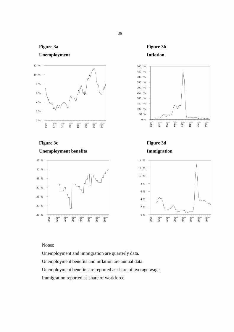
the Israeli labor market went through dramatic changes in the 1990s. Figures 3a through 3d

depict the evolution of the main variables over time.

3.II.1. Demand factors.

3.II.1.a. Total productivity

For a downwards sloping demand curve, competitive behavior requires that along the

demand curve wages equal the marginal product of labor while shifts in the curve are

caused by changes in total factor productivity (A) and the capital stock (K). We find

evidence for a short run effect of the total factor productivity only for the period following

the stabilization program of 1985 (Table 1, equations 3 through 5). We also found a

significant effect of the capital stock when we introduced the two-period lagged change in

the capital labor ratio16 (Table 1, equations 4 and 5). It can thus be argued that there was a

significant change in the labor market. Prior to 1985 trade unions were stronger and wages

largely determined by central negotiations. The adjustment of wages to productivity and to

changes in the capital labor ratio was made much more slowly, taking into account the

16 By the two-period lagged capital labor ratio we avoid the simultaneity problem of having labor in the denominator of the capital stock.

18

long-term trend The effect of this slow adjustment to long-run productivity is captured by

the error–correction term, which is indicates that, discounting all other variables,

adjustment to equilibrium takes almost two years. The decline in the power of trade unions

and wage negotiations at plant or individual level may have strengthened the link between

wages and productivity in the short-run. It may thus be argued that wage bargaining

models may be unlikely to account for recent developments in the labor market. On the

other hand the results is more consistent with the efficiency wages model that suggests that

real wages are increased to induce productivity.17 In sum, based on the effect of

productivity, it seems that in the 1970s the Israeli labor market’s behavior in the short run

could be modeled along the lines of a bargaining (insiders-outsiders) model, but that the

1990s can be better explained by the neo-classical, or efficiency wage competitive model.

3.II.1.b Producer prices

In the short-run, the ratio of producer to consumer prices (PYPC) appears to be significant

in the pre-stabilization period suggesting that during the high inflation period it contributed

substantially to the variance of real wages. This may be explained by the distortions in the

price system which were stronger during the inflationary period. A number of studies

allude to higher price variability and other relative-price distortions during the period of

high inflation. Our results contribute to these findings first by showing that these effects

were also significant in the labor market and second by showing that they contribute to

distort not only goods allocation but also labor allocation.

17 Granger causality tests tend to support causation running from wages to total factor productivity.

19

In the post stabilization period, there were smaller deviations in the short run between

producer and consumer prices. This phenomenon may be also accounted for by the

reduction in government subsidies on numerous consumption items that prevailed in the

1970s and early 1980s and also to the decline in the use of price controls which were also

prevalent in the 1970s. Both sorts of intervention drove a wedge between the subsidized or

controlled consumer prices and producer prices.

3.II.1.c. Structural change.

In the theoretical section we alluded to theories that suggest that skill biased structural

change caused by productivity changes in ‘high tech’ sectors have a differential effect on

labor markets. In particular changes in demand for skilled labor face a steep labor supply

curves, meaning that in the short-run wages will rise much faster in that sector (with little

change in employment) whereas they will not change much in the unskilled sector. We

therefore included the ratio of unemployment of skilled (13 years of education and 16

years from 1988) versus unskilled (UR) to test the hypothesis that the recent structural

change had short term effects on real-wages. The estimation results suggest that this effect

is constant during the whole sample. Note that Card, Kramarz and Lemieux (1999) find

little evidence for the effect of structural change on unemployment. This result is

consistent with the high-tech based growth of the Israeli economy which is characterized

as running against an inelastic skilled-labor supply curve.

20

3.II.1.d. Minimum wages

Minimum wages have been the subject of numerous studies. Some argue that they have a

significant impact on the labor market and natural unemployment, others argue that their

effects are marginal. In Israel, there was a voluntary minimum wage agreement since the

1970s, but, minimum wage legislation began only in 1987 and therefore we can not obtain

estimates to their affect on real wages for the entire sample. The major increases in

minimum wages occurred since 1994. Unfortunately, during the 1990s minimum wages

and unemployment benefits were raised in a similar manner – the two variables are

correlated. While we can not introduce both unemployment benefits and minimum wages

in the same regression, the results of a regression with minimum wages alone indicate that

minimum wages play a significant role in explaining the deviation of real wages from their

long-run equilibrium in the 1990s.18 Nevertheless we prefer the introduction of

unemployment benefits since the contribute more to explaining the variance of real wages

and are more consistent with the theory we employ.

3.II.2. Supply Factors

According to the model, the effect of labor supply on real wages can be identified only in

the short run. In the long run, changes in labor supply affect employment.

18 The following result was obtained: For equations 4 and 5 we obtained a coefficient of 0.3 and T value of 2.8 on the minimum wage lagged three periods. The other coefficients do not change significantly. However the adjusted R square falls from 0.68 to 0.64.

21

3.II.2.a. Mass Immigration.

In the early 90s Israel saw a massive inflow of immigrants from the former Soviet Union.

The Israeli population increased by some 10% within a couple of years. The effect of this

large increase in the labor force, given a short run downwards sloping demand for labor

curve, was to reduce real wages significantly either directly or perhaps more strongly via

expectations of future (after absorption) increases in the labor supply. As expected, our

regressions results (Table 1 equations 3-5) report a large and significant negative effect of

the immigration wave (Imm) on real wages in the 1990s.

3.II.2.b. Unemployment benefits.

Unemployment benefits (UB) affect the reservation wage of labor and their participation in

the labor force. In the long run, unemployment benefits affect the level of natural

unemployment while in the short run it also affects real wages. Unemployment benefits in

Israel are a relatively new phenomenon. While they existed since the early 1970s, their

level was low – some 20% of the average wage. Collecting unemployment benefits was

also stigmatized in Israeli society. In the 1980s, unemployment benefits increased to cover

40% of the average wage, and in recent years the level of coverage went up to 50% of the

average wage19. Moreover, the number of workers collecting these benefits increased

19 There were minor changes in minimum wage regulations and coverage. The rise in the level of coverage to 50% of the average wage is mainly due to a composition effect: More previously employed higher paid workers are claiming these benefits.

22

dramatically. It is no longer perceived as socially inappropriate to receive unemployment

benefits.

Given the marked changes in the coverage and the recourse to unemployment benefits we

hypothesize that the effect of this variable on real wages is bound to become more

significant in recent years. Indeed, we do not find a significant effect of unemployment

benefits in the regression we ran for the whole sample and for the 70s and 80s. Moreover,

comparison of regressions 3, 4 and 5 suggests that the rise in the effect of unemployment

benefits came at the expense of labor-market forces – the effect of lagged unemployment

(U), reflecting labor-market pressures - loses significance altogether. In the absence of

unemployment benefits rising unemployment acts to restore real wages to their equilibrium

levels. However, recourse to unemployment benefits mitigates this effect. The results

suggest that in the 70s and early 80s unemployment benefits were effectively bellow the

implicit reservation wages of potential labor market participants. In recent years these

benefits constitute an explicit measure of the reservation wages in Israel. Altogether, the

rising significance of unemployment benefits is a major structural change in the Israeli

labor market, a change that makes it resemble more closely European labor markets. In this

paper we report the short term effects of unemployment benefits on real wages. However,

given the significance we observe, it is very likely that unemployment benefits may

provide a significant explanation for the rise in the natural unemployment rate in Israel in

the 90s.

23

3.III. Nominal rigidities.

3.III.a. Unexpected inflation

As argued in the methodology section, the ex-post real wage we measure may deviate from

the ex-ante market clearing real wage. The difference between ex-post (actual) real wages

and the ex-ante market clearing real wage is the result of unexpected changes in inflation

and nominal wage rigidities that do not allow for the immediate adjustment of nominal

wages to unexpected changes in the price level. In the absence of perfect foresight,

inflation surprises are negatively correlated with actual real wages. However, different

methods of formulating expectations of inflation rate may have different affects on real

wages. The more adaptive are the expectations, the longer is the deviation of actual real

wages from ex-ante real wages. The weights of the lagged coefficients not only determine

the length of convergence of real wages following an inflation surprise, but also their

volatility in that interval.

The results obtained indicate, that expectations of inflation changed a little with the shift to

lower inflation rates in the 90s. For the entire sample and especially for the 70s and 80s we

obtain a significant negative coefficient on current change in inflation (CPI) whereas for

the 90s we obtain a significant coefficient and higher on the current change in inflation and

a lower coefficient on lagged inflation. This seems to imply that expected inflation, as

captured by our estimated model changed somewhat over time.

24

We can extract the structure of expectations in the following way. Holding everything else

constant, our model assumes that the change in nominal wages accounts for expected

inflation, e

dtdw π= , and we can write the following equation for the entire sample based on

equation 1 in Table 1.

)(34.0)(28.0 211 −−− −−−−=− ttttttw πππππ&

Substituting the change in nominal wages for expected inflation and rearranging we obtain:

21 34.066.072.0 −− ++∆= tttet ππππ

Compared with a benchmark based on perfect foresight expected inflation:

1−+∆= ttet πππ

We note the (relatively low) adaptive nature of the estimated expectations. 20

For the 1990s we are fortunate enough to have expected inflation as measured in the bonds

market and can therefore calculate a measure of unexpected inflation.21 We find (Table 1,

equation 5) that unexpected inflation (UEI) enters the regression with a coefficient close to

0.6. In Figure 4 we compare the expectations generated from our estimated regression

(Table 1, equation 4) and those obtained generated from the bond market. The overall

trends are similar, albeit the expectations calculated directly from the labor market show

greater volatility. This disparity is perhaps more of a reflection of the shortcomings of our

20 Expected inflation as calculated from the wage equations is stable throughout the period. Even for the 90s we obtain a very similar (albeit less adaptive) expected inflation:

21 3.07.06.0 −− ++∆= tttet ππππ

21 Expected inflation is calculated by computing the yield difference between linked and unlinked, of equal duration, government bonds.

25

ability to model expected inflation than any shortcomings of labor to employ the

information on expected inflation provided by the capital market. Note that the time

horizon for the estimated expected inflation is one quarter while that derived from the

capital market is for one year. It is quite natural for the shorter horizon series to exhibit

greater volatility than that of the longer run.

We wish to stress that this result suggests that wage setting is done in a rational manner

and that there are no money illusion effects. The results obtained also suggest that nominal

wage contracting is prevalent in the Israeli labor market, contrary to the findings of Keane

for the U.S. (1993).

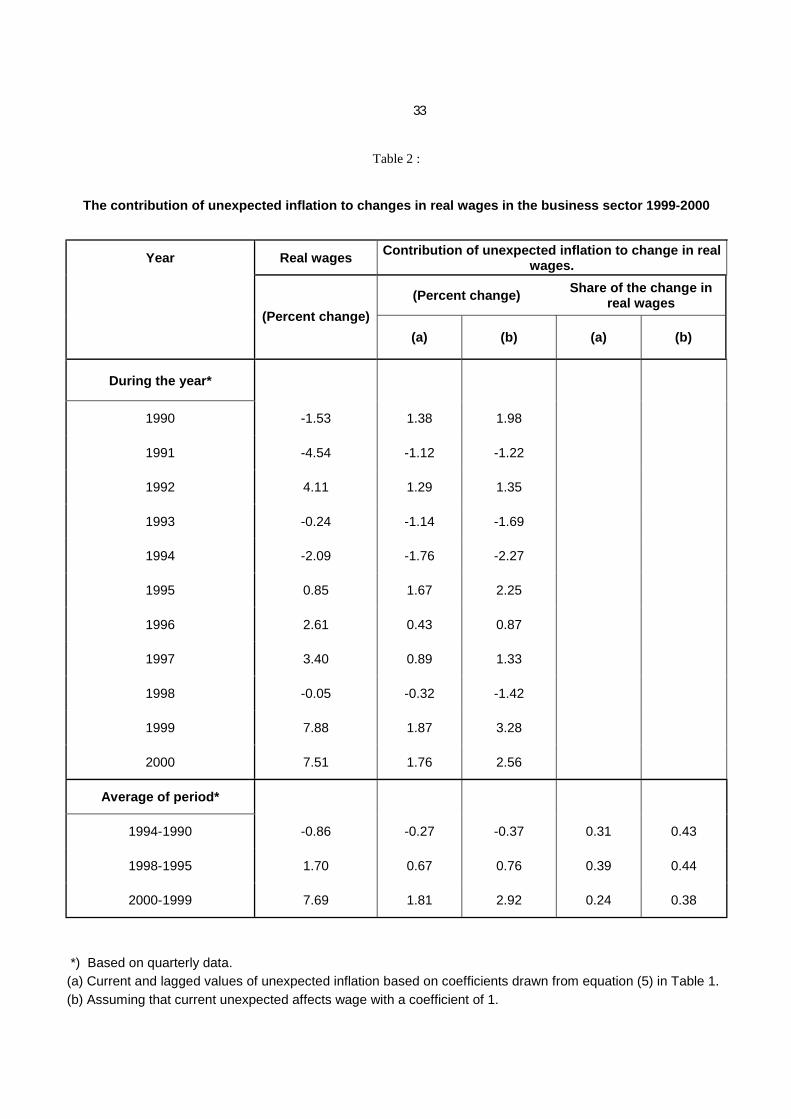
In Table 2 we show the short-term contribution of unexpected inflation to the change in

real wages. Averaging over the period of loose monetary policy, as measured by the real

interest rate (1990-1994) and tight monetary policy (1995-1998) we show that unexpected

inflation explains a third to 40% of the change in real wages, with a smaller effect during

recent years (1999-2000). This exercise provides an alternative approach to assessing the

cost of disinflation. It shows the contribution of unexpected disinflation to the short run

deviation of real wages from equilibrium and the subsequent rise in unemployment.

3.III. b. Cost of living adjustment.

During the 70s and 80s cost of living (COL) adjustments played a significant role in the

adjustment of wages to inflation. It was sometimes argued that these arrangement

introduced real wages rigidities. Our findings show that the effect of COL adjustment

(indexation) is temporary, it is reversed within 6 months (3 months in the post-stabilization

26

period). The significant contribution of the COL arrangements might have been in

affecting the formation of expectations on inflation. The COL acted as insurance against

inflation surprises22, thereby reducing the myopic element in the inflation expectations

formation. We therefore find some support for Taylor (1979) who argued that in order to

mitigate unemployment costs the COL should continue during disinflation allowing for

‘negative’ indexation.

3.IV. Labor market adjustments

Although an attempt was made to specify the demand and supply factors that affect real

wages in the short-run, there are still unspecified shocks that can be captured by the

unemployment rate which acts as a measurement of labor market disequilibrium. We found

a significant effect for a trend variable of unemployment – the change in unemployment

over 6 months, rather than one quarter. The importance of this variable declines over time,

perhaps due to the rise of the importance of unemployment benefits that introduce a

rigidity in the adjustment of real wages, especially in situations of excess supply of labor.

Rather than exerting pressure on real wages, the unemployed prefer to collect

unemployment benefits.

22 See Shiffer (1999) and Liviatan (1982).

27

3.V. Institutional rigidities.

It has been argued that owing to its large share and leading role, the public sector has an

effect on the private sector wages (mainly wages of professionals). Therefore, changes in

wages in the public sector that are not always based on market variables may affect wages

in the private sector. We ran regressions that included the public sector wage but they had

no such effect within any time lag.

3.VI. Unobserved dynamics – the error correction term.

Our model specifies a long-term real wage equation based on a neo-classical model of the

labor market. We showed that over the long-run real wages in Israel attain their long term

equilibrium values. The dynamics of the short run may be captured by specified demand

and supply factors, the lagged short term effects of the variables that determine wages in

the long run (productivity). It may be possible that we can not fully specify the short-run

forces that lead wages back to their long run equilibrium. The error correction term (RES),

based on the errors of the long –term cointegrating equation is used to capture the back-to-

equilibrium dynamics. We find a significant error correction term in our regression of a

magnitude suggesting that convergence to the long-run following a disturbance is achieved

after 8-16 quarters (depending on the regression).23 This adjustment process does not seem

too prolonged. In the 1990s the adjustment period is about 10 quarters which is slower than

what we observed for the 1970s.

23 Adjustment is defined as the return to the 95% level of equilibrium real wages.

28

5. Conclusions

The transition of the labor market from one characterized by centrally negotiated wages to

a more competitive one, albeit augmented by minimum wage and unemployment benefits

legislation, has so far probably caused it to work less smoothly as the effect of new

institutions outweighs the steps taken towards a more competitive labor market. Is this an

outcome of a transition period to be followed by a more flexible operation of the labor

market in the future or are we entering a new era of slow adjustment of the labor market

and longer deviations from the equilibrium real wage of the long-run, such as in Europe?

These questions have important bearing on the rate of unemployment, income inequality

and government policies.

29

References

Artstein Yael, (1997), Wage Rigidity in Israel: Institutions versus Market Forces. Ph.D.

Thesis, Tel-Aviv University. (in Hebrew)

Bender Keith A. and Iioannis Thesdossiou, (1998), “International Comparisons of the Real

Wage-Employment Relationship.” Journal of Macroeconomics 20(4) pp. 811-19.

Blanchard Olivier and Lawrence F. Katz, (1997), “What we Know and do not Know about

the Natural Rate of Unemployment.” Journal of Economic Perspectives, 11(1), pp.

51-72.

Card David, Kramarz Francis and Thomas Lemieux (1999) “Changes in the Relative

Structure of Wages and Employment: a Comparison of the United States, Canada

and France. Canadian Journal of Economics August , pp. 843-77.

Clamfors Lars, (1990), “Wage Formation and Macroeconomic Policy in the Nordic

Countries: A summary”, in Clamfors Lars ed. Wage Formation and

Macroeconomic Policy in the Nordic Countries, Oxford, pp.. 11-62.

Jacobson Tor, Anders Verdin and Anders Warne, (1998) “Are Real Wages and

Unemployment Related.” Economica 65(1), pp. 69-96.

30

Jullien Bruno and Pierre Picard, (1998), “A Classical Model of Involuntary

Unemployment: Efficiency Wages and Macroeconomic Policy.” Journal of

Economic Theory , 78(2) pp. 263-85.

Layard Richard, Stephen Nickel and Richard Jackman (1991), Unemployment, Oxford.

Liviatan Oded, (1982), “The Development of the Cost of Living Agreement and other

Wage Components,” Economic Review, 115, pp. 349-357. In Hebrew.

Michael P. Keane, (1993), “Nominal Contracting Theories of Unemployment: Evidence

from Panel Data.” American Economic Review 83(4), pp. 932-52.

Sachs, Jeffrey D., (1979) “Wages, Profits, and Macroeconomic Adjustment: A

Comparative Study.” Brookings Papers on Economic Activity; 2(79), pp. 269-319.

Shiffer Zalman, (1999), “The Cost of Living Adjustment as a Tool Protecting Real Wages

from Inflation Surprises,” Research Dept. Bank of Israel Discussion Paper, in

Hebrew.

Taylor, John B. (1979) “Staggered Wage Setting in a Macro Model.” American Economic

Review; 69(2), pp.1

31

Variables List: explanation of symbols

A total factor productivity (Solow – residual).

CPI consumption price index.

Imm immigration rate (of total population).

Indexation cost of living adjustment.

K capital stock.

K/L capital stock to labor ratio.

L labor input.

PYFPC ratio of producer (at factor prices) to consumer prices.

PYPC ratio of producer to consumer prices (at market prices).

RES the residual estimated from the long run equation (error – correction term).

U unemployment rate.

UB unemployment benefits to average wage ratio.

UEI unexpected inflation.

UR ratio of unemployment of skilled versus unskilled workers.

Y/L product per labor unit (labor productivity).

Note: The prefixed “D” denotes the difference operator.

32

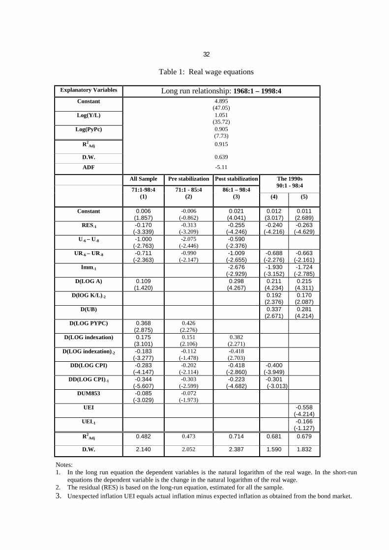
Table 1: Real wage equations

Explanatory Variables Long run relationship: 1968:1 – 1998:4

Constant 4.895 (47.05)

Log(Y/L) 1.051 (35.72)

Log(PyPc) 0.905 (7.73)

R2Adj 0.915

D.W. 0.639

ADF -5.11

All Sample Pre stabilization Post stabilization The 1990s 90:1 - 98:4

71:1-98:4 (1)

71:1 - 85:4 (2)

86:1 – 98:4 (3) (4)

(5)

Constant 0.006 (1.857)

-0.006 (-0.862)

0.021 (4.041)

0.012 (3.017)

0.011 (2.689)

RES-1 -0.170 (-3.339)

-0.313 (-3.209)

-0.255 (-4.246)

-0.240 (-4.216)

-0.263 (-4.629)

U-6 – U-8 -1.000 (-2.763)

-2.075 (-2.446)

-0.590 (-2.376)

UR-6 – UR-8 -0.711 (-2.363)

-0.990 (-2.147)

-1.009 (-2.655)

-0.688 (-2.276)

-0.663 (-2.161)

Imm-1 -2.676 (-2.929)

-1.930 (-3.152)

-1.724 (-2.785)

D(LOG A) 0.109 (1.420)

0.298 (4.267)

0.211 (4.234)

0.215 (4.311)

D(lOG K/L)-2 0.192 (2.376)

0.170 (2.087)

D(UB) 0.337 (2.671)

0.281 (4.214)

D(LOG PYPC) 0.368 (2.875)

0.426 (2.276)

D(LOG indexation) 0.175 (3.101)

0.151 (2.106)

0.382 (2.271)

D(LOG indexation)-2 -0.183 (-3.277)

-0.112 (-1.478)

-0.418 (2.703)

DD(LOG CPI) -0.283 (-4.147)

-0.202 (-2.114)

-0.418 (-2.860)

-0.400 (-3.949)

DD(LOG CPI)-1 -0.344 (-5.607)

-0.303 (-2.599)

-0.223 (-4.682)

-0.301 -3.013)(

DUM853 -0.085 (-3.029)

-0.072 (-1.973)

UEI -0.558 (-4.214)

UEI-1 -0.166 (-1.127)

R2Adj 0.482 0.473 0.714 0.681 0.679

D.W. 2.140 2.052 2.387 1.590 1.832

Notes: 1. In the long run equation the dependent variables is the natural logarithm of the real wage. In the short-run

equations the dependent variable is the change in the natural logarithm of the real wage. 2. The residual (RES) is based on the long-run equation, estimated for all the sample. 3. Unexpected inflation UEI equals actual inflation minus expected inflation as obtained from the bond market.

33

Table 2 :

The contribution of unexpected inflation to changes in real wages in the business sector 1999-2000

Year Real wages Contribution of unexpected inflation to change in real wages.

(Percent change) Share of the change in real wages

(Percent change) (a) (b) (a) (b)

During the year*

1990 -1.53 1.38 1.98

1991 -4.54 -1.12 -1.22

1992 4.11 1.29 1.35

1993 -0.24 -1.14 -1.69

1994 -2.09 -1.76 -2.27

1995 0.85 1.67 2.25

1996 2.61 0.43 0.87

1997 3.40 0.89 1.33

1998 -0.05 -0.32 -1.42

1999 7.88 1.87 3.28

2000 7.51 1.76 2.56

Average of period*

1994-1990 -0.86 -0.27 -0.37 0.31 0.43

1998-1995 1.70 0.67 0.76 0.39 0.44

2000-1999 7.69 1.81 2.92 0.24 0.38

*) Based on quarterly data. (a) Current and lagged values of unexpected inflation based on coefficients drawn from equation (5) in Table 1. (b) Assuming that current unexpected affects wage with a coefficient of 1.

34

Notes: Long run share obtained from the estimation of the long run real wage (Table 1). The level of the shares is biased downwards as wages data do not include indirect benefits. GDP refers to business sector output.

Figure 1Share of Labor Income of GDP - Israel: 1968:1-1998:3

35%

37%

39%

41%

43%

45%

47%

49%

51%

1968:1

1969:1

1970:1

1971:1

1972:1

1973:1

1974:1

1975:1

1976:1

1977:1

1978:1

1979:1

1980:1

1981:1

1982:1

1983:1

1984:1

1985:1

1986:1

1987:1

1988:1

1989:1

1990:1

1991:1

1992:1

1993:1

1994:1

1995:1

1996:1

1997:1

1998:1

Labor share long-run labor share*

35

Notes: Quarterly data. Data refer to the business sector.

Figure 2Real Wages and Output per Worker, Israel: 1968:1-1998:3

1968

:1

1968

:4

1969

:3

1970

:2

1971

:1

1971

:4

1972

:3

1973

:2

1974

:1

1974

:4

1975

:3

1976

:2

1977

:1

1977

:4

1978

:3

1979

:2

1980

:1

1980

:4

1981

:3

1982

:2

1983

:1

1983

:4

1984

:3

1985

:2

1986

:1

1986

:4

1987

:3

1988

:2

1989

:1

1989

:4

1990

:3

1991

:2

1992

:1

1992

:4

1993

:3

1994

:2

1995

:1

1995

:4

1996

:3

1997

:2

1998

:1

Real Wages Output per worker

36

Figure 3a Figure 3b

Unemployment Inflation

Figure 3c Figure 3d

Unemployment benefits Immigration

Notes:

Unemployment and immigration are quarterly data.

Unemployment benefits and inflation are annual data.

Unemployment benefits are reported as share of average wage.

Immigration reported as share of workforce.

0 %

2 %

4 %

6 %

8 %

10 %

12 %

1968

: 11972

: 11976

: 11980

: 11984

: 11988

: 11992

: 11996

0 %

50 %

100 %

150 %

200 %

250 %

300 %

350 %

400 %

450 %

500 %

1968

: 11972

: 11976

: 11980

: 11984

: 11988

: 11992

: 11996

0 %

2 %

4 %

6 %

8 %

10 %

12 %

14 %

1968

: 11972

: 11976

: 11980

: 11984

: 11988

: 11992

: 11996

25 %

30 %

35 %

40 %

45 %

50 %

55 %

1968

: 11972

: 11976

: 11980

: 11984

: 11988

: 11992

: 11996

37

Figure 4

Expected Inflation: 1990:1-1998:3

Notes: Expectations are measured in annual terms. Expectations from wage equation using coefficients from Table 1 equation 4.

Figure 5

Effect of Unexpected Inflation on Real Wages: 1992:1-1998:3

Notes: Simulated wage calculated by taking the actual real wage in period (t-1) and subtracting from it unexpected inflation.

0%

5%

10%

15%

20%

25%

30%

1990:1

1991:1

1992:1

1993:1

1994:1

1995:1

1996:1

1997:1

1998:1

Wage equation Bond market

8.10

8.15

8.20

8.25

1992:I 1992:IV 1993:III 1994:II 1995:I 1995:IV 1996:III 1997:II 1998:I

Simulated real wage actual real wage

38

Appendix

Table A1 Estimated Cobb-Douglas production function 1968:1 – 1998:3

Explanatory Variables Long run relationship

Constant 0.642 (0.975)

Time Trend 0.003 (5.62)

Inflation -0.013 (-2.71)

Log(K) 0.343 (6.56)

Log(L) 0.651 (8.08)

R2Adj 0.991

D.W. 0.71

ADF -3.95 (-3.45)

Table A2 Long –Run real wage equations: 1968:1 – 1998:3

Assuming demand curve for labor is downwards sloping

Explanatory Variables Constant 6.663

(101.396)

Log(A) 0.863 (8.058)

Log(PYPC) 0.739 (5.149)

Log(UB) 0.792 (4.119)

R2Adj 0.777

D.W. 0.824

ADF -4.63 (-3.51)

39

Table A3

Short –Run real wage equations: 1977:2 – 1998:3

Assuming demand curve for labor is downwards sloping

All Sample Pre stabilization

Post Stabilization

The 1990s

77:2-98:3 (1)

77:2 - 85:4 (2)

86:1 - 98:3 (3)

90:1 – 98:3 (4) (5)

Constant 0.007 (1.921)

0.011 (0.848)

0.019 (6.171)

0.015 (3.204)

0.013 (2.459)

RES-1 -0.143 (-2.594)

-0.228 (-2.000)

-0.261 (-5.040)

-0.262 (-3.758)

-0.276 (-3.831)

U-6 - U-8 -1.041 (-2.703)

-2.649 (-2.097)

-0.327 (-1.746)

UR-6 - UR-8 -0.549 (-1.673)

-1.021 (-3.514)

-0.932 (-2.425)

-0.789 (-1.880)

Imm-1 -2.749 (-3.794)

-2.320 (-2.833)

-2.128 (-2.408)

D(LOG A) 0.226 (3.136)

0.218 (4.812)

0.219 (4.884)

D(UB) 0.549 (4.983)

0.527 (4.716)

D(LOG PYPC) 0.334 (2.372)

0.447 (1.798)

D(LOG indexation) 0.186 (3.031)

0.152 (1.674)

D(LOG indexation)-2 -0.204 (-3.357)

-0.168 (-1.810)

DD(LOG CPI) -0.312 (-4.348)

-0.271 (-2.468)

-0.270 (-1.697)

-0.289 (-3.119)

DD(LOG CPI)-1 -0.347 (-5.346)

-0.316 (-2.081)

-0.139 (-2.588)

-0.267 (-2.868)

DUM853 -0.076 (-2.689)

-0.052 (-1.155)

UEI -0.467 (-3.424)

UEI-1 -0.262

(-1.889) AR(1) -0.380

(-2.874) 0.341

(1.830) 0.407

(2.199) R2

Adj 0.497 0.464 0.712 0.660 0.658

S.E. 0.026 0.036 0.014 0.008 0.008

D.W. 2.062 1.867 2.105 2.161 2.263

Notes: 1. In the long run equation the dependent variables is the natural logarithm of the real wage. In the

short-run equations the dependent variable is the change in the natural logarithm of the real age. 2. The residual (RES) is based on the long-run equation (Table A2), estimated for all the sample. 3. Unexpected inflation UEI equals actual inflation minus expected inflation as obtained from the

bond market.

40

Table A4

Real wage equations : the long-run relationship

Based on annual data

National accounts data The works data 1961 - 1999 1968 – 1999 1968 - 1998 Explanatory

Variables (1) (2) (3) (4) (5)

Constant 6.698 (44.375)

6.782 (39.955)

5.799 (23.996)

5.663 (17.699)

4.733 (22.731)

Log(Y/L) 0.955 (29.361)

0.943 (25.660)

1.146 (22.191)

1.180 (17.324)

1.065 (20.387)

Log(PYPC) 0.970 (4.376) 1.318

(6.716) 0.923 (4.280)

Log(PYFPC) 0.386 (2.788) 0.683

(4.828)

Statistics:

Adj. R2 0.959 0.949 0.943 0.919 0.935

D.W. 0.494 0.460 0.803 0.665 0.716

A.D.F -2.176 -2.489 -3.324 -2.923 -3.247

Elasticity of substitution 1.05 1.06 0.87 0.85 0.94

Note: The dependent variable is the natural logarithm of the real wage.