THE DESIGN AND MANUFACTURING PROCESSES OPTIMIZATION OF...
116
UNIVERSITY OF MICHIGAN THE DESIGN AND MANUFACTURING PROCESSES OPTIMIZATION OF A CAR’S B-PILLARS By Zheng Shen Liang Xi Ying Luo Yue Jian ME 555-12-03 Winter 2012 Final Report The design and manufacturing processes optimization of a car‘s B-pillars was investigated in detail. This project aims at optimizing the B-pillars to reduce the cost to build lightweight B- pillar structure and decrease the structure weight subjected to feasible manufacturing process and satisfactory crash worthiness in side impact. The B-pillars system has been divided into four significant subsystems, this is, lightweight structure design, hot stamping optimization, optimization of laser welding process and cost optimization. Each subsystem is optimized to minimize its own objective function subjected to its own constraints. In the subsystems, at least one of analysis, Finite Element simulation and metamodel (stepwise and linear regression and neural networks) is applied to construct the corresponding model. Finally subsystems are integrated and optimized as a single optimization problem, namely All-in-One (AIO) approach. The project terminates by finding an optimal design with the tradeoff among low cost, lightweight and applicable manufacturing ABSTRACT
-
Upload
truongtram -
Category
Documents
-
view
216 -
download
0
Transcript of THE DESIGN AND MANUFACTURING PROCESSES OPTIMIZATION OF...

UNIVERSITY OF MICHIGAN
THE DESIGN AND MANUFACTURING
PROCESSES OPTIMIZATION OF A CAR’S B-PILLARS By
Zheng Shen
Liang Xi
Ying Luo
Yue Jian
ME 555-12-03
Winter 2012 Final Report
The design and manufacturing processes optimization of a car‘s B-pillars was investigated in
detail. This project aims at optimizing the B-pillars to reduce the cost to build lightweight B-
pillar structure and decrease the structure weight subjected to feasible manufacturing process
and satisfactory crash worthiness in side impact. The B-pillars system has been divided into
four significant subsystems, this is, lightweight structure design, hot stamping optimization,
optimization of laser welding process and cost optimization. Each subsystem is optimized to
minimize its own objective function subjected to its own constraints. In the subsystems, at
least one of analysis, Finite Element simulation and metamodel (stepwise and linear
regression and neural networks) is applied to construct the corresponding model. Finally
subsystems are integrated and optimized as a single optimization problem, namely All-in-One
(AIO) approach. The project terminates by finding an optimal design with the tradeoff among
low cost, lightweight and applicable manufacturing
ABSTRACT

Contents
3
Contents
1 Design Problem Statement................................................................................................................. 8
2 METAMODEL-BASED LIGHTWEIGHT STRUCTURE OPTIMIZATION OF B-
PILLAR UNDER SIDE IMPACT LOADING --- Zheng Shen ............................................................... 9
2.1 Simplified Structure Model ...................................................................................................... 9
2.2 Simplified Structure Model .................................................................................................... 10
2.3 Nomenclature ......................................................................................................................... 12
2.4 Mathematical Models ............................................................................................................. 13
2.5 Model Analysis ...................................................................................................................... 14
2.6 Optimization Methodology .................................................................................................... 14
2.6.1 Metamodeling Method ....................................................................................................... 14
2.6.2 Design of Experiment ........................................................................................................ 15
2.6.3 Monotonicity Analysis ....................................................................................................... 17
2.6.4 Optimization Method ......................................................................................................... 18
2.7 Numerical Result ................................................................................................................... 18
2.8 System-level Tradeoffs .......................................................................................................... 20
2.9 Discussions ............................................................................................................................ 20
3 METAMODEL-BASED HOT STAMPING OPTIMIZATION OF B-PILLAR --- Ying Luo ....... 22
3.1 Problem Statement ................................................................................................................. 22
3.2 Nomenclature ......................................................................................................................... 25

Contents
4
3.3 MATHEMATICAL MODEL ................................................................................................ 27
3.3.1 Objective function .............................................................................................................. 27
3.3.2 Design Variables ................................................................................................................ 27
3.3.3 Parameters .......................................................................................................................... 27
3.3.4 Constraints ......................................................................................................................... 29
3.3.5 Summary of Model ............................................................................................................ 31
3.4 Optimization Model Analysis ................................................................................................ 32
3.4.1 Metamodeling .................................................................................................................... 32
3.4.2 Design of Experiment and Simulation ............................................................................... 32
3.4.3 Dependent Analysis ........................................................................................................... 34
3.4.4 Monotonicity Analysis ....................................................................................................... 34
3.4.5 Activeness Analysis ........................................................................................................... 35
3.4.6 Numerical Results .............................................................................................................. 36
3.4.7 Parameter Analysis ............................................................................................................ 38
3.5 System Trade-Off ................................................................................................................... 39
3.6 Problem Discussion ............................................................................................................... 39
4 Optimization of Laser Welding Process .......................................................................................... 40
4.1 Background ............................................................................................................................ 40
4.2 Subproblem Description ........................................................................................................ 41

Contents
5
4.3 Nomenclature ......................................................................................................................... 42
4.4 Mathematical Model .............................................................................................................. 43
4.4.1 Objective Function ............................................................................................................. 43
4.4.2 Constraints ......................................................................................................................... 44
4.4.3 Metamodel ......................................................................................................................... 46
4.4.3.1 .................................................................................................................. 46
4.4.3.2 ................................................................................................................. 49
4.4.4 Model summary ................................................................................................................. 51
4.4.5 FDT Analysis ..................................................................................................................... 54
4.4.6 Monotonicity Analysis ....................................................................................................... 54
4.5 Optimization Study ................................................................................................................ 57
4.5.1 Process Description ............................................................................................................ 57
4.5.2 Algorithm Compare ........................................................................................................... 58
4.5.3 Parametric Studies.............................................................................................................. 61
4.5.4 Discussion of results .......................................................................................................... 62
5 COST OPTIMIZATION OF B-PILLAR PRODUCTION .............................................................. 63
5.1 Problem Statement ................................................................................................................. 63
5.2 Nomenclature ......................................................................................................................... 64
5.2.1 Parameters: ......................................................................................................................... 64

Contents
6
5.2.2 Variables ............................................................................................................................ 66
5.3 Mathematical Model .............................................................................................................. 67
5.3.1 Constraints ......................................................................................................................... 67
5.3.2 Modeling ............................................................................................................................ 69
5.3.2.1 The cost in the stamping process, .............................................................................. 70
5.3.2.2 The cost in the welding process ................................................................................. 71
5.3.2.3 Material cost ............................................................................................................... 73
5.3.2.4 Model Sumary ............................................................................................................ 73
5.4 Optimization Model Analysis ................................................................................................ 75
5.4.1 Monotonicity Analysis ....................................................................................................... 75
5.5 Numerical Optimization ......................................................................................................... 77
5.6 Discussion of Results ............................................................................................................. 80
6 System Integration Study ................................................................................................................. 81
6.1 System Interactions ................................................................................................................ 81
6.2 Problem Formulation ............................................................................................................. 82
6.3 Optimization Approaches ...................................................................................................... 84
6.4 Dicussion................................................................................................................................ 85
7 REFERENCES ................................................................................................................................ 86
8 Apprendix ........................................................................................................................................ 88

Contents
7
8.1 MATLAB Code for the structure optimization ...................................................................... 88
8.2 MATLAB Code for the stamping optimization ................................................................... 101
8.3 MATLAB Code for the welding optimization ..................................................................... 110
8.4 MATLAB Code for the cost optimization ........................................................................... 116

8
1 Design Problem Statement
Pillars are the vertical or near vertical supports of an automobile's window area or greenhouse —
designated respectively as the A, B, C or D-pillar moving in profile view from the front to rear. In
American and British English, the pillars are sometimes referred to as posts (A-post, B-post etc.).This
project focus on the design and manufacturing processes optimization of a car‘s B-pillars.
The division of the system and the team member responsible for each subsystem is as follows:
Table 1.1 Subsystem
Subsystem Team member
Metamodel-based Lightweight Structure Optimization of
B-Pillar under Side Impact Loading
Zheng Shen
Metamodel-based Hot Stamping Optimization of B-Pillar Ying Luo
Optimization of Laser Welding Process Liang Xi
Cost Optimization of B-Pillar Production Yue Jian

9
2 METAMODEL-BASED LIGHTWEIGHT STRUCTURE OPTIMIZATION OF B-
PILLAR UNDER SIDE IMPACT LOADING --- Zheng Shen
2.1 Simplified Structure Model
Structure Structure design is the first step in the whole developing and manufacturing process of a B-
pillar. A B-pillar is mainly involved in side impact crash and roll over crash conditions (Figure 1). In
order to limit the injury of passengers during the impact, and ensure the side door could open for
evacuation after the crash, a B-pillar should be of high strength to limit the intrusion and deformation
(Figure 2). Meanwhile, it also needs to cut down the total mass for lightweight design purpose.
a) Roll over crash conditions b) Side impact crash conditions
Fig. 1 Two main crash conditions that a B-pillar will get involved in
a) Deformation mode sketch b) Deformation in FE simulation
Fig. 2 the deformation mode of a B-pillar in side impact
Side impact
force
Upper of the B-
pillar
Maximum
Intrusion
Maximum
Intrusion

10
Due to the geometric complexity, a B-pillar is formed in several components, and then gets jointed by
welding process. In order to decrease the total mass, different materials are applied in different
components according to their requirements of mechanics behavior. In nowadays, even one
component can be break down into different pieces with different materials to maximally reduce the
redundant weight and make fully use of material properties (Figure 3).
a) Assembly components of B-pillar b) Outer components divided into
partitions with different materials
Fig. 3 Assembly components design of a B-pillar
2.2 Simplified Structure Model
a) Before crash simulation b) deformation during crash simulation
Fig. 4 Simplified FE Structure Model with side barrier
In this project, a simplified FE structure model is generated. The main frame structure of passenger
cabin is constructed with distributed nodal mass loading (0.6 ton on the front wheel axis, 0.4 ton on
the rear wheel axis) to simulate the real situation of a compact passenger sedan. The test sample of B-

11
pillar is represented by a simplified square-box welded up by 2 U-section bars. And the outer bar is
actually formed with tailor-welded blank method, with which the lightweight design is accessible by
applying different materials to different pieces of panels. The B-pillar is mounted on the main frame
structure on the inner sheet at both ends by rigid-body connection.
a) Intersection design of B-pillar b) Tailor welded blanks design of outside of B-pillar
Fig. 5 Geometric design variables of B-pillar
The side impact scenario is built up according to IIHS side-impact protocol with certain simplification.
The initial impact velocity of main frame is 5566.6 mm/s. The barrier with the same size of that in real
IIHS test is instead made with rigid material.Main design variables are focus on the geometry size and
material selection of B-pillar.
The material for components of B-pillar is selected as high strength steel with properties shown in
following tables.
Table 1 Material property
ID Young's
Module
Poisson
Ratio Density
Yield
Stress
Plastic
curve
Mpa Ton/mm^2 Mpa Strain Stress
HS 1400 210000 0.3 7.89E-09 411 0 411
7.27350-3 404.20001
0.030141 465.73001
0.15315 548.25
0.2 615.38
0.22 800
0.2461 1444.4
𝑙𝑙
𝑙𝑚2
𝑙ℎ
𝑎
ℎ𝑙
𝑏
𝑑 𝑐
𝑡
12
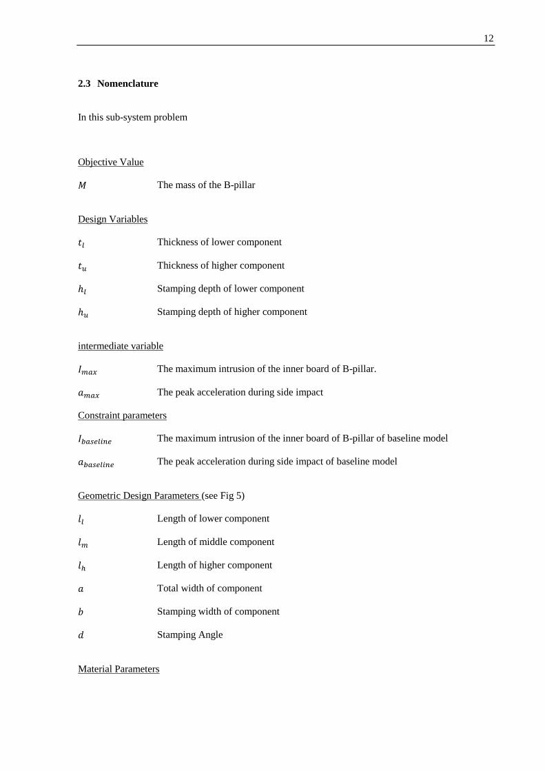
2.3 Nomenclature
In this sub-system problem
Objective Value
The mass of the B-pillar
Design Variables
Thickness of lower component
Thickness of higher component
ℎ Stamping depth of lower component
ℎ Stamping depth of higher component
intermediate variable
The maximum intrusion of the inner board of B-pillar.
The peak acceleration during side impact
Constraint parameters
The maximum intrusion of the inner board of B-pillar of baseline model
The peak acceleration during side impact of baseline model
Geometric Design Parameters (see Fig 5)
Length of lower component
Length of middle component
ℎ Length of higher component
Total width of component
Stamping width of component
Stamping Angle
Material Parameters

13
Sy Material Yield Strength
E Material Elongation
Strain of the Material
Stress of the Material
Density of material
Number of spot-welds
The failure stress of spot-weld
2.4 Mathematical Models
The ultimate goal in this structure design problem is to minimize the total mass of the B-pillar, and
ensure the crashworthiness performance is better than the baseline model. The crashworthiness
performance, including maximum side intrusion and maximum side impact acceleration, can be
obtained during FE-simulation. Due to the complexity of plastic deformation, the mathematical model
of intrusion can only be obtained in surrogate model created on the result of preliminary DoE study.
Min ∑
(Equation 5.1)
Subject to ℎ (Equation 5.2)
ℎ ℎ ℎ (Equation 5.3)
ℎ ℎ (Equation 5.4)
(Equation 5.5)
(Equation 5.6)
ℎ (Equation 5.7)
(Equation 5.8)
(Equation 5.9)
(Equation 5.10)
(Equation 5.11)
ℎ (Equation 5.12)

14
2.5 Model Analysis
It is helpful to do the preliminary analysis of mathematic model before solving it using optimization
method. The monotonicity analysis will tell the trend of model and guide the local computation. The
problem discussed here is a typical lightweight structure optimal design problem, and the structure
mass is the monotonically increasing function of component thickness and stamping depth. In the
preliminary study, the mass function is obtained as
ℎ ℎ ℎ ℎ ℎ ℎ (Equation 5.13)
Where ,
2.6 Optimization Methodology
2.6.1 Metamodeling Method
Metamodel-based optimization is an effective approach for engineering design problems, especially
when the problem has highly complex relationships between variables, constraints and objects.
The common approach to access Metamodel-based optimization includes several following steps (
Fig. 6):
1. Define the optimization problem: objectives, constraints and design variables.
2. Generate samples of design variables using Design of Experiment method, including Latin
hypercube method, Uni-variant method, Orthogonal arrays method, Central composite methods
etc.
3. Conduct numerical simulations using sampled points as input, and extract the interesting values of
responses.
4. Use the extracted result values to generate the metamodel. Techniques for metamodeling includes
regression, neural network, etc.
5. Assess the predictive capabilities of the metamodel by testing samples in unsampled design space.
If the model is ill constructed, refine the model by these testing samples.
6. Search the optimization over the design space using the constructed metamodel. If the
convergence is achieved, stop and output the result, otherwise, refine the model by increasing
samples.required.

15
Fig. 6 Metamodel-based optimization procedure
2.6.2 Design of Experiment
To generate the metamodel, several real results are required to do the training. Samples are constructed
in Catia, meshed and prepared in Hypermesh. FE simulations are conducted using LS-Dyna and run
on CAEN advanced computing center. Each sample uses 8 clusters and 30 minutes to compute. A
batch script is generated to extract the interesting data out of result automatically. Matlab is called to
do the post-processing, including integration and smooting.
In the first round of DoE study, quasi-full-factorial sampling method is applied to gather global
information of design space. The variables and their levels are shown in Table 2
Thus, there are 75 samples generated and run in side impact scenario via Finite Element Simulation.
And the validation result shows good consistency between metamodel and real situation whenh_l is
close to 3 sampling levels, that means it goes well along the surface of t_l and t_2 once h_l is fixed
close enough to its sampling levels. However, in the dimention of h_l due to the sparse levels in h_l
dimension, the metamodeling results turn to vary dramatically, showing obvious over-fitting problem.
Yes
No No
Yes
Define the
optimization problem
DoE study over the
design space
FE simulation at
sampling points
Refine the
model by more
Construct the metamodel
usually not analytical
Validate the model Perform the optimization
Check the convergence
Output

16
Table 2 Quasi-full-factorial sampling
Design Variables Level 1 Level 2 Level 3 Level 4 Level 5
ℎ
2
In order to improve the quality of metamodel, a second round of 25 samples is generated using Latin
Hypercube Sampling method and added into the training data. In the meantime, the spread of radial
basis functions of neural network is controlled at 1.5, and the total amount of neurons is limited at 50.
Getting trained in such way, the new metamodel shows higher training error but the validation error is
remarkably improved, which shows in Table 3.
Table 3 Validation result for improved Metamodel
Design
Variables Sample_1 Sample_2 Sample_3 Sample_4 Sample_5 Sample_6
ℎ 39.4649 41.9507 40.2964 35.7155 44.0470 37.8566
2.2368 1.0475 1.3636 1.5958 2.0580 1.8682
2 1.7757 1.0225 2.1880 1.9923 1.6392 2.3058
Error of max
intrusion 0.1094 0.1347 0.0816 0.0023 0.0134 0.0838
Error of peak
acceleration 0.1582 0.1693 0.0272 0.1412 0.1509 0.0054

17
2.6.3 Monotonicity Analysis
Fig. 7 Intrusion response surface model
Fig. 8 Acceleration response surface model
In the monotonicity analysis based on metamodel, the highly nonlinear response of maximum
intrusion, peak acceleration are shown in fig.7 and fig 8. And they together with the structure mass in
fig. 9 have different trends in performance according to 3 design variables. Thus there shall be several
local optimization results of structure mass inside the design space under the nonlinear constraints of
intrusion and acceleration.

18
Fig. 9 Structure mass response surface model
2.6.4 Optimization Method
The matlab function fmincon is applied to solve the optimization problem. Since the numerical
metamodel has no analytical function, the Active-Set Optimization method is used to find the local
optimal. In order to search around the whole design space, the fmincon is iterated for 5 times, and
each time the 6 initial searching points are generated again by Latin Hypercube Sampling method.
2.7 Numerical Result
The 1st round optimization result is shown in Table 4, the average iteration time is 35.
Table 4 Comparison of 1st round optimization results
Design
Variables Sample_1 Sample_2 Sample_3 Sample_4 Sample_5 Baseline
ℎ 38.3712 36.4330 40.6616 37.0970 38.8566 40.0000
1.6236 2.3895 1.7008 2.0780 2.2735 1.80000
2 2.2770 1.4531 1.0000 1.9966 1.2300 2.40000
max
intrusion 82.9471 76.6247 83.0011 82.1529 74.5444 83.4110
peak acc. 5.4619 5.2423 5.5377 5.8168 5.8037 5.8169
Mass 0.0035 0.0027 0.0019 0.0033 0.0024 0.0038

19
From the result, it is easy to tell the notable local optimum phenomenon, which proves that the model
is highly nonlinear and non-monotony. The 3-D plot of solution space (Fig. 6) also reveals such
property in the metamodel of constraint functions. Another reason that leads the result to be non-
converged is that the unequal constraints from Baseline model is relatively slack so that there are more
local optimums that satisfy the constraints, and the optimization algorithm will stop at those local
optimums.
Fig. 10 The local optimum situation in problems with nonlinear constraint
The figure above (fig.10) sketches the local optimum situation caused by nonlinear constraint
function. From the figure we can see, a tighten constraint value will eliminate those local optimum
with higher object value and force the optimization converge to a lower solution, which is more likely
the global optimum. According to this understanding, in the second round optimization running, a
tighten upper bound of baseline model is set at max intrusion = 70.000, and max acc. = 5.5000. Then
the result is shown in Table 5, the average iteration time is 37.
In this result, a better convergence is achieved at , and another better
local minimal is at . These results are then checked in FE simulation. The
design point at has a simulation result at ,
which is worse than the design constraints. However, the minimal at has
a performance at , which is quite close to the result from metamodel. In
comparisons of these samples with of closer samples that are used in DoE study, their simulation
results are relatively closer to sample results, showing reasonable continuity of response in local
regions. The false result at from metamodel is probably caused by local
overfitting of metamodel.

20
Table 4 Comparison of 2nd
round optimization results
Design
Variables Sample_1 Sample_2 Sample_3 Sample_4 Sample_5 Baseline
ℎ 40.8301 44.6990 44.6989 41.6077 44.7009
2.3763 1.8800 1.8800 2.0050 1.8800
2 1.5988 1.5442 1.5442 1.0000 1.5441
max
intrusion 64.7752 70.0000 70.0000 70.0000 70.0000 70.000
peak acc. 5.3588 5.5000 5.5000 4.4169 5.5000 5.5000
Mass 0.0030 0.0028 0.0028 0.0021 0.0028
In the optimization running afterward, more results are founded closely around at
, which are encouraging to choose this local optimum as a reasonable
global solution under given constraints.
2.8 System-level Tradeoffs
The subsystem of structure optimization is closely related to other subsystem problems in this topic.
Currently the 3 design variables ℎ , , 2 are only bounded by empirical design regions. While in
reality, ℎ , , 2 all will strictly constrained by forming process of stamping (subsystem 3), the
, 2 will affect the quality of spot-welding (subsystem 2), and the total mass of the structure as well
as the manufacturability of such design in stamping process and spot-welding jointing will be
observably constrained by the manufacturing cost control (subsystem 4).
2.9 Discussions
The optimal design of vehicle structure is a classical nonlinear optimization problem. According to
different targets, the nonlinearity can be in the constraint (when optimizing weight) or object function
(when optimizing the crashworthiness performance). This nonlinearity is due to the complex geometry
and its behavior under high speed impact loading, which is very hard to decompose and get the
analytical function. Metamodel method shows a good performance when trying to solve such
problems, which is also demonstrated in this subsystem. To ensure the accuracy of metamodel, a well-
designed DoE study is quite necessary to train the model with least losing of information in real

21
scenarios. And if possible, an automatic iteration of DoE and model training will be even better. A
derivative-free optimization/searching method then will find the local optimum over the metamodel.
The problem of converging into different local minimums is still very common over the metamodel,
especially when the real problem is highly nonlinear. Thus, a good global searching method is still
needed.
From above, we can see that metamodel-based method has several steps to conduct and is very costly
of time in sample preparation and of computation in metamodel generation. A popular research in this
area is trying to optimize the whole procedure: using the least samples to generate the best fitting
metalmodel. And in real engineering application, another important problem for such research method
is to setup the design space, which highly requires expert-knowledge in such domain.

22
3 METAMODEL-BASED HOT STAMPING OPTIMIZATION OF B-PILLAR --- Ying
Luo
There are two basic approaches on the design of EVs: conversion- design and purpose-built design.
Either an existing ICE vehicle is converted into an electric vehicle by replacing the propulsion system,
while keeping the general structure, or a completely new vehicle is designed to specifically fit the
purpose of using electric propulsion. Both methods and current supermini class models will be
introduced. Those ICE models designed with alternative propulsion taken in mind will be included in
the purpose-built section. The overview presents selected EV models‘ performance, body design and
choice of drive train equipment as well as their packaging and safety performance. To demonstrate the
difficulties and measures taken in the field of EV crash safety the selection is focussed on purpose-
built EVs that stand out for their performance, size, weight, design or safety concepts. EG-class M1
vehicles, which need to meet the standard safety regulations and demand a regular driving licence,
were preferred.
Additional models and details are summarized in table 1 in the appendix, which is neither claimed to
be complete in all details nor in the range of current models, due to the lack of published details on the
new models and the abundance of EVs currently introduced. It will, however, provide an overview
over current developments in mini EVs. Unfortunately there is only very few information released on
crash data of EVs.
3.1 Problem Statement
The automotive industries have been interested in light weighted components and the safety as well as
the quality of vehicles for years. With years of development in this industry people have found out that
both weight reduction and performance improvement can be achieved by optimizing structure design,
enhancing the properties of materials and improving the process of manufacturing. As a key
manufacturing process, stamping plays an important role in the entire manufacturing process
especially welding and the quality and performance of the vehicles. Additionally, stamping also
implies limitations and prospects of the structure geometry and material selection, contributing to the
design stages. It has been proved that properly control of the stamping process and carefully design of
the die geometry could enhance the material formability, allowing more design possibility. Moreover,
properly designed stamping could directly increase the accuracy of the final structure, and help to
modify the quality of the vehicles.

23
This optimal subsystem aims at decreasing the manufacturing cost of the automotive B-pillar by
minimizing the maximum punch force during stamping and maximize the formability of the blank at
the same time, taking consideration of the limits of material formability during the process, the trade-
off with the structure geometric design stage and industrial requirements. Moreover, the effects to
welding process are also considered in the entire optimization system.
Punch force, according to previews studies, has been proved to be affected by four main factors, which
namely are blank holder force, friction conditions and the punch stroke. Nevertheless, some other
factors such as the final thickness of the blank that is introduced to avoid crack at the edge of the
structure and minimize the total mass the B-pillar is also important.
Fig.1 B-pillar in vehicles: a) the outside and inside B-pillar; b) the simplified structure of B-pillar; c)
the dimensional parameters of simplified B-pillar
Fig.2 Hot stamping process in industry
As presented in the above figure, B-pillar of the vehicle is simplified as a U shape shown in Fig1.b,
most of the geometric characteristics of the structure shown in Fig1.a is given by the design stage. In

24
the stamping process, a rectangular blank with properly designed dimensions is assembled between a
die and two blank holders. A punch with designated geometries then moves down with a constant
speed to form the final shape. In order to reduce noises from non-considered factors, the manipulation
of the blank is assumed to be the same on the direction as the pillar goes. Therefore, only cross-section
of the sample is analyzed. During this process, four factors (i.e. the blank holder force, the coefficient
of friction, the punch stroke and the final thickness of the blank) are used as the four variables, and the
properties of the material as well as the initial dimensional factors are considered as parameter.
Fig.3 The setup of stamping process

25
3.2 Nomenclature
Objective Value
The mass of the B-pillar
Material Properties
Sy Yield Strength
St Tensile Strength
Y Young‘s Modulus
Poisson's ratio
E Elongation
K Strength coefficient
n Strength exponent
l Elongation of the material at stamped temperature
intermediate variable
td Designed thickness of B-pillar
to Initial thickness of the blank
tf Final thickness of B-pillar
h Stroke of the punch
hd Designed depth of B-pillar
R Designed radial of die
Designed angle 1 of B-pillar
Wo Original width of blank

26
Top width of B-pillar
2 Bottom width of B-pillar
Area of the each blank holder
Machine setting
Maximum punch force
Blank hold force
The coefficient of friction between the blank and die
Maximum acceptable friction coefficient
Minimum acceptable friction coefficient
Geometric Design Parameters (see Fig 5)
Length of lower component
Length of middle component
ℎ Length of higher component
Total width of component
Stamping width of component
Stamping Angle
Material Parameters
Sy Material Yield Strength
E Material Elongation
Strain of the Material
Stress of the Material
Density of material
Number of spot-welds
The failure stress of spot-weld

27
3.3 MATHEMATICAL MODEL
3.3.1 Objective function
The aim of the subsystem is to minimize the punch force during stamping.
ℎ 2 ℎ ℎ
The objective function can be achieved by performing simulation of stamping process accounting for
the different variables, and by carrying out the DOE (design of experiment), a series of punch force
depending on the change of variables are recorded.
3.3.2 Design Variables
The decision variables are selected based on previous study investigating factors that could affect
punch force most significantly, and some factors that have influence on the formability of metal.
Decision Variables:
Blank hold force in stamping
The punch coefficient of friction
h Punch stroke
Final thickness of B-pillar
3.3.3 Parameters
Material Properties:
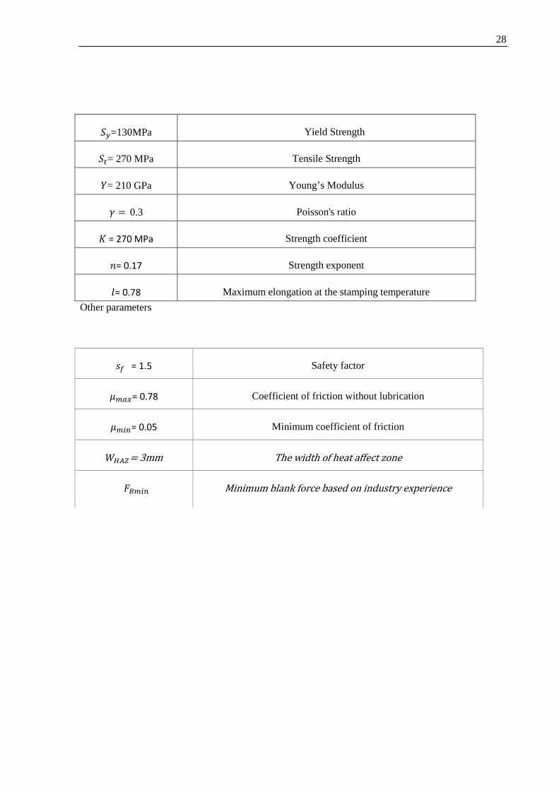
28
=130MPa Yield Strength
= 270 MPa Tensile Strength
= 210 GPa Young‘s Modulus
0.3 Poisson's ratio
= 270 MPa Strength coefficient
= 0.17 Strength exponent
= 0.78 Maximum elongation at the stamping temperature
Other parameters
= 1.5 Safety factor
= 0.78 Coefficient of friction without lubrication
= 0.05 Minimum coefficient of friction
= 3mm The width of heat affect zone
Minimum blank force based on industry experience

29
Geometric factors
3.3.4 Constraints
All the variables and parameters that help to perform a simulation should result a stamping model
satisfying the material limits, the geometric limits, physical limits as well as industrial limits. At the
same time, the limits introduced by other subsystem should also be considered.
For the material properties requirement, and based on the simulation results, the maximum normal and
shear stress could be derivate and mustn‘t exceed the material tensile stress with accounting for the
safety factor.
(equation 3.1)
The geometry limits are caused by the geometric design of the structure as well as the welding process
requirements. Based on the geometric relationship, the upper limit of the punch stroke is determined.
2
2
2 ℎ
2 (equation 3.2)
ℎ
( )
ℎ (
)
= 2 mm Designed thickness of B-pillar
ℎ = 35 mm Designed depth of B-pillar
Designed angle of B-pillar
= 340 mm Original width of blank
= 140 mm Top width of B-pillar
2 = 60 mm Bottom width of B-pillar
= 60 mm2 Area of the each blank holder

30
In practice, the blank holder force is applied to avoid wrinkling during stamping. Therefore, the blank
holder force could not be too small. On the other hand, this limit is set to avoid damage and wear for
the stamping machine. Hence, the blank holder force should not be excessively large, which could lead
fracture of the material. The maximum blank holder force is therefore roughly calculated by
considering the surface shear stress raised by friction.
FB F ’ (Equation 3.3)
FB F’ - (Equation 3.4)
FBmin FB F (Equation 3.5)
Another important consideration of the stamping process is the formability of the material, which
could be approximated by the allowed minimum thickness after stamping. In order to avoid failure
during the stamping process, and based on the physical requirement that the blank volume should be
constant during the whole process, the lower and upper bound of the final thickness could be
determined:
(Equation 3.6)
(Equation 3.7)
Moreover, the coefficient of friction should be consistent to the industrial used value
(Equation 3.8)
(Equation 3.9)

31
3.3.5 Summary of Model
By simplifying the model and eliminating the obvious redundant equalities, the summary
model could be built.
Objective
Function: (ℎ ) 2 (Equation 3.10)
Subject to (Equation 3.11)
2
2
ℎ
(Equation 3.12)
ℎ
( )
ℎ (
)
(Equation 3.13)
(Equation 3.14)
(Equation 3.15)
(Equation 3.16)
(Equation 3.17)
(Equation 3.18)
(Equation 3.19)
(Equation 3.20)
(Equation 3..21)

32
3.4 Optimization Model Analysis
3.4.1 Metamodeling
As an effective approach for engineering design problems, metamodel-based optimization is widely
used in the problems with significantly complex relationships among variables, parameters, constrains
and objects. The typical step of processing metamodeling method is show as follows:
Fig 3.4 Steps of metamodeling
3.4.2 Design of Experiment and Simulation
In order to obtain simulation samples with variable values more entirely and randomly spread in the
design domain, Latin hypercube method was used to determine the sample values. The model was
built and simulated using Abaqus and the correlate values were reported when simulation finished.
Two methods have been applied to obtain the relationship between the objective function (and certain
constraints) and variables. Firstly the recorded data were analyzed by regression and therefore find out
the error level. By adjusting the range and order of the polynomial function, and the error was
minimized, and the form of the function was obtained. Since the relationship between the object and
Yes
No No
Yes
Optimization problem
definition
DoE analysis in the
feasible domain
FE simulation using
sampling points
Refine the
model by more
Construct the metamodel
Validate the model Perform the optimization
Check the convergence
Output

33
variables is not clear, all the variables were scaled to the same range to ensure that their influence
would not be affected by their value level. Secondly the determined polynomial function was analyzed
using stepwise algorithm to eliminate the less important ones. By combination of these two method,
the objective function was achieved:
2 ℎ
(rsq = 0.80)
(Equation 3.22)
Similarly, one constraint function, namely the maximum stress of the blank, was obtained without
scaling:
(rsq = 0.78)
(Equation 3.23)
Five randomly selected samples were selected and simulated to validate the polynomial functions
obtained.
Table 3.1 Validation form
Variables Sample_1 Sample_2 Sample_3 Sample_4 Sample_5
7.3 5.9 13.4 10.6 9.2
2.1 1.6 1.9 2.4 1.7
0.6 0.1 0.3 0.5 0.7
36.1 40.5 44.9 48.3 52.4
Error 19.8% 14.3% 15.7% 25.6% 20.1%

34
3.4.3 Dependent Analysis
Table 3.2 Variable dependent analysis
Variables 𝐟 𝟐 𝟑 𝟒 𝟓 𝟔 𝟕 𝟖 𝟗
𝑭𝑩𝑯𝑭
𝒕𝒇
𝛍
𝒉
3.4.4 Monotonicity Analysis
The monotonicity analysis is performed as shown in Table. 10.

35
Table 3.3 Monotonicity analysis
Variables 𝐟 𝟐 𝟑 𝟒 𝟓 𝟔 𝟕 𝟖 𝟗
𝑭𝑩𝑯𝑭 + ? + + -- --
𝒕𝒇 + -- + -- --
𝛍 ? + + + -- --
𝒉 -- + + -- --
Activity
Active
for
&
Active
for
Active
for
Active
for
Active
for
Active
for
According to the analysis above, it is obvious that all variables correlating to different constraints have
at least one upper and one lower bound, implying a well boundedness of the problem. Meanwhile,
since some of the constraints has non-linear functions, there will be some extra boundedness.
3.4.5 Activeness Analysis
As discussed above, the problem is well bounded. Now it is necessary to check if all constraints are
active. Firstly from the monotonicity analysis table, is upper bounded by both and and
lower bounded by and . Based on the monotonicity principles, at least one of and are
active.
:
:
Obviously, that is a stronger boundary than , so that can be defined as inactive constraint.
By applying this method to check all constraints, the activeness could be determined and the analyze
results are show in the monotonicity table.

36
3.4.6 Numerical Results
This problem is to find a best trade-off between the minimizing the punch force and maximizing the
blank formability. Therefore, different optimization could be found based on different consideration of
the weight of each objective (i.e. minimizing punch force, maximizing the punch stroke and
minimizing the final thickness).
By considering the three objective as equally important, the optimization of the problem could be
found out by applying Fmincon-interior-point algorithm, which shows an optimized result with
different initial guess. The Following are four guesses of the initial guesses:
Scenario 1:
Initial guess Final value Value of the
objective after
optimization
Number of
interations 𝑭𝑩𝑯𝑭 7.04kN 9.41kN
0.52
45 𝒕𝒇 1.6mm 1.98mm
𝛍 0.64 0.33
𝒉 37.99mm 43.77mm
Scenario 2:
Initial guess Final value Value of the
objective after
optimization
Number of
interations 14.16kN 9.42kN
0.51
34
1.8mm 1.97mm
0.17 0.32
45.83mm 43.78mm
37
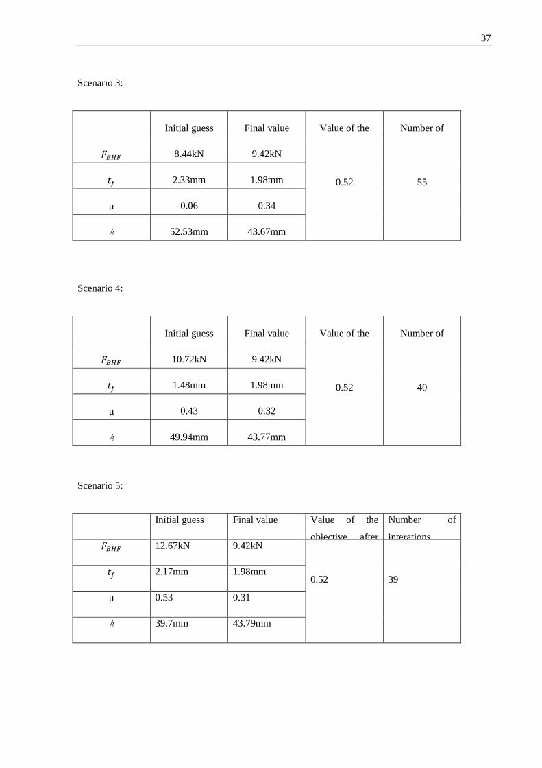
Scenario 3:
Initial guess Final value Value of the
objective after
optimization
Number of
interations 8.44kN 9.42kN
0.52
55 2.33mm 1.98mm
0.06 0.34
52.53mm 43.67mm
Scenario 4:
Initial guess Final value Value of the
objective after
optimization
Number of
interations 10.72kN 9.42kN
0.52
40 1.48mm 1.98mm
0.43 0.32
49.94mm 43.77mm
Scenario 5:
Initial guess Final value Value of the
objective after
optimization
Number of
interations 12.67kN 9.42kN
0.52
39 2.17mm 1.98mm
0.53 0.31
39.7mm 43.79mm

38
3.4.7 Parameter Analysis
With all other parameters fixed and only change the weight factor of each sub-objective function, the
results changed slightly as shown below:
Initial guess Final value Value of the
objective after
optimization
Number of
interations
12.67kN 8.77kN
0.61
29 2.17mm 2.01mm
0.53 0.38
39.7mm 41.72mm
Initial guess Final value Value of the
objective after
optimization
Number of
interations
12.67kN 7.86kN
0.47
47 2.17mm 1.72mm
0.53 0.23
39.7mm 45.98mm

39
However, when to change the other parameters including such as the initial dimension of the blank,
the solution tends not valid, and the functions obtained by simulation and regression have been
significantly changed. For that reason, it can just conclude the this optimization solution is only valid
for these specific siduation.
3.5 System Trade-Off
The subsystem of stamping optimization is closely related to other subsystems especially the structure
optimization subsystem. The dimensional variables are bounded by the design requirements, and the
welding subsystem also implied some limits to the final thickness. Meanwhile, the initial thickness of
the blank is leaked to the material cost in the cost subsystem. Finally, the punch force is a limit for the
cost subsystem to estimate the tool life.
3.6 Problem Discussion
There are some problems can be observed in this problem. Firstly when the parameters linked to the
stamping process (such as the blank initial dimension) change, the entire optimization would fail.
Besides, the error in validation is not low enough. There are several possible reasons that can explain
the phenomenon. One of the most possible reasons is that simple polynomial function cannot express
relationships between the variables and punch force. For example, according to the previews studies,
with the change of the die dimension, the tendency of the change of the punch force would be different
with punch stroke increasing (i.e. in some experiments, the punch force would increase with the punch
stroke increasing, while in some other cases, there will be a decreasing when punch stroke reach a
certain value). Meanwhile, with theoretical mechanism analysis, there should be at least one
exponential relationship between the punch force and coefficient of friction. In conclusion, the
relationship between the variables and objective function are too complex to process a linear
regression analysis. On the other hand, the number of samples of this problem is possibly not enough
to present a right relationship between the variables and objective functions. In the future work, it is
recommended that more samples are simulated and other metamodeling-based method such as neural
net work could be used to find a more nonlinear relationship.

40
4 Optimization of Laser Welding Process
4.1 Background
Laser welding has been widely used in the manufacturing processes of vehicles due to its obvious
advantages. The focused laser beam possesses the high power density, the low and localized energy
input, the ability to be precisely controlled, to name only a few. These benefits of laser beam could
result in a high depth-to width ratio, a small heat-affected zone, minimal distortion and residual
stresses. Thus, various vehicles structures including B-pillar (Fig. 4-1) prefer to use laser welding [6,
7].
Fig. 4.1: Laser Beam welding of B-Pillar
In the case of B-pillars, outer and inner plates are jointed together using spot laser welding. This joint
has to possess enough shear strength in order to avoid fracture during the side collision. The joint
strength of the laser welds depends on the weld joining area [8], penetration and residual stress which
are largely determined by the properties of materials, the parameters of laser welding input parameters,
including output power, welding speed, focal position, shielding gas and position accuracy [9]. In
addition, the heat input and heat affect zone affect the welding quality due to their influence of causing
distortion during or after the welding process.

41
4.2 Subproblem Description
For simplified model, this individual study focuses on optimizing the laser welding variables such as
beam power, beam exposure time, incident angle of the beam (shown in Fig. 4-2), distance between
two adjacent spot welds and total number of spot welds in order to maximize the joint strength and to
keep the heat input at reasonable range.
The variables of laser power, exposure time and incident angle exert effect on the geometry of spot
welds, especially for beam width and depth of penetration. Those are highly likely to decide the
strength of single spot weld. At the same time, the strength of weld in B-pillar is the comprehensive
result of the strength of the total number of spot welds. Distance between two neighbouring spot
welds has direct relationship with the number of spot welds. Thus, the strength function can be
expressed with those variables.
(a)
(b)
Figure 4.2 Geometry of spot weld, B-pillar and properties of laser
The constraints can be obtained through the requirement of welding and physical phenomena. It will
be discussed in detailed in the following parts.

42
4.3 Nomenclature
S Safety factor
Shear Stress During Collision
[] Acceptable Shear Stress for Weld
F The Tensile Force During Collision
n Total Number of Spot Welds per Side
BW Bead Width
p Beam Power
Dp Depth of Penetration of The Weld
a Incident Angle
t Exposure Time
Absorption Coefficient
L Length of The B-Pillar
d Distance Between Two Adjacent Spot Welds
h Thickness of the Workpiece
Q Heat Input for Single Weld
Qmax Acceptable Heat Input for Single Weld
Ultimate Tensile Strength of the High Strength Steel
Safety Factor That Depends on the Potential Consequences of Failure

43
4.4 Mathematical Model
During side collision, the joint connecting inner and outer B-pillar primarily bears shear stress due to
the dissimilar plastic deformation between these two B-pillars. The resulting tremendous shear stress
may cause the failure of the weld. In order to reduce the possibility of failure of the joint, the joint
strength has to be strong enough to overcome the huge shear stress in the process of crash.
The joint strength has direct relationship with the bearing capacity. Thus, the primary objective of this
subsystem is to maximize the bearing capacity under the reasonable heat input and the diminutive heat
affected zone.
Figure 4.3 Force Analysis in B Pillar
4.4.1 Objective Function
Even through the actual stress distribution over the joint is very compressive, an estimate of the value
of stress in the joints can be done under the assumptions that stress distribution is uniform along the
welds and residual stress of the joints is ignored. This assumption makes sense due to the fact that the
distribution of residual stress is pretty complex and difficult to be calculated; more importantly,
residual stress could not be obvious if some measures are taken during the process of design and
manufacturing [10].
The shear stress across the weld is depends on the force F, the across area of the weld, and the total
number of spot welds. Here, we just use the to represent the shear stress over the weld, and
this term will be discussed in detail in the metamodel.
The relationship between and is given by:
(Equation 4.1)

44
The following acceptable stresses can be assumed for the strength of welded joints for static load [11].
Actually during the side collision, the load changed dramatically, while [τ] can be estimated by using
the coefficient 3.5 in the denominator.
(Equation 4.2)
By the nature of safety factor, , this means, has to be larger than so that the weld
would not be damaged. Usually, the value of S is larger, the strength of the weld is stronger. Thus, the
objective function of this subsystem can be represented by equation (7.3):
(Equation 4.3)
4.4.2 Constraints
The depth of penetration depends on laser power p, exposure time t and incident angle [12]. The exact
form of will be explored in the metamodel. In order to produce an acceptable weld, the
depth of penetration should not be less than the thickness of single plate:
ℎ (Equation 4.4)
The heat input has direct relationship with the beam power, beam exposure time and the absorption
coefficient. It can be calculated by:
(Equation 4.5)
The large heat input would cause distortion of B pillar and enlarge the heat-affected zone, which has
adverse effect on the strength of spot weld. Here, we limit to 1.5 kJ. So, another constraint is
given by:

45
(Equation 4.6)
The total number of spot weld and distance between them is limited by the length of B pillar:
(Equation 4.7)
(Equation 4.8)
The welding operations are performed using 2 kW continuous wave ND:YAG laser. Limited by the
capacity of the laser equipment, the constraint for the power is given by:
(Equation 4.9)
Welding quality depends on the beam exposure time to a large extent. Too short beam exposure time
leads to the insufficient weld; on the other hand, with too long beam exposure time, the welding bead
will be damaged resulting in the poor quality of spot bead. Here, the range for beam exposure time
remains the same as that of the reference [12]:
(Equation 4.10)
The incident angle of the beam also has effect on the weld geometry. Welding with straight beam ( 90°
beam incident angle) may damage the optics by back reflection of the beam. So the scope of beam
incident angle is kept the same as that of the reference [12]:
(Equation 4.11)
In addition, the distance between spot weld affects the strength of B pillar. When the distance is larger
than 70 mm, the strength of B pillar reduces obviously. At the same time, this distance is restricted by
the design of B pillar, this is 24 mm. So the range of distance is given by:
(Equation 4.12)

46
4.4.3 Metamodel
Linear and quadratic polynomial equations for predicting the depth penetration and the bead width
were developed. A stepwise method in Matlab was used to fit the second order polynomial equation
(4.13) in the reference [12] data and to identify the relevant model terms.
∑ ∑ (Equation 4.13)
4.4.3.1
The stepwise method is to build the quadratic form for the function of depth of penetration (DP) with
respect to exposure time (t), beam power (p) and incident angle (a). The figure below is results for
stepwise and the detailed code is attached as Appendix. From the results of stepwise (figure 4.4), it can
be found that the significance for the terms of t, a, t2 and a2 is worst and can be removed. Regression
method is utilized to find out the coefficient of the rest terms. Finally, the equation is shown as
equation (4.14):
2
(Equation 4.14)

47
Figure 4.4 the results of stepwise
To verify the equation, the curve of the function is plotted for each parameter, and the dots in the
figure below are original data.
Figure 4.5 Depth of penetration against beam exposure time
Figure 4.6 Depth of penetration against beam power

48
Figure 4.7 Depth of penetration against incident angle.
From the figure 5-7, the curve is in good agreement with the original data, so the metamodle is
acceptable.

49
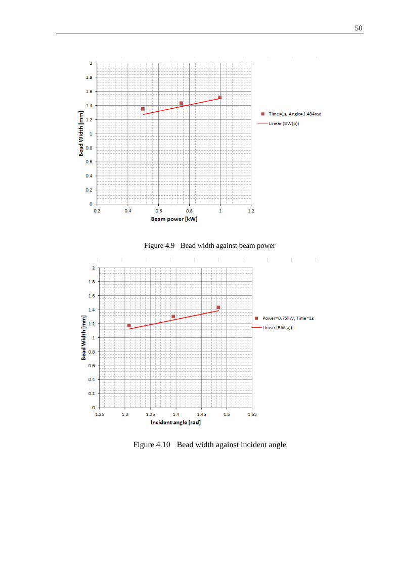
4.4.3.2
As for the function of bead width with the variables of beam power, incident angle and beam exposure
time, the stepwise method can be also use to identify the significant terms, a and p×t, and then the
equation (4.15) are obtained using the regression method:
(Equation 4.15)
Verification has been taken and the curves are in good agreement with the original data (figure 8-10).
Figure 4.8 Bead width against beam exposure time
The highest tensile force is parameter from design system. Here F=20 kN, but more investigation is
required to verify this value.
50
Figure 4.9 Bead width against beam power
Figure 4.10 Bead width against incident angle
51
2
(Equation 4.16)
2
(Equation 7.17)
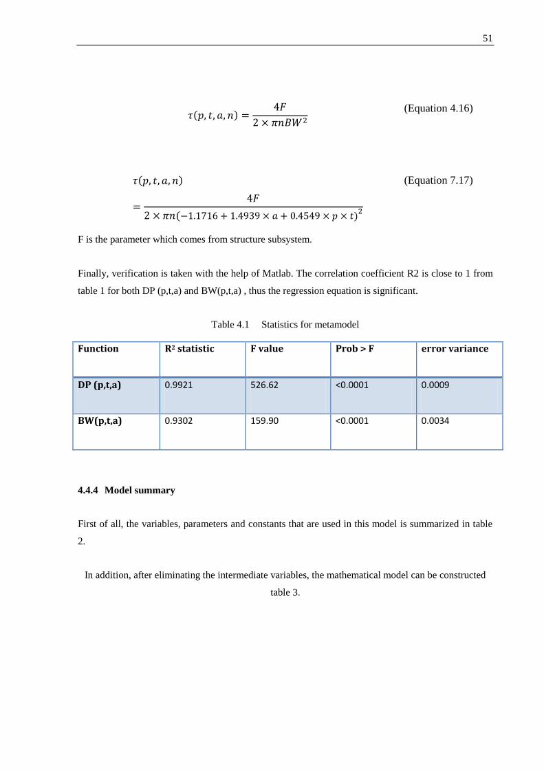
F is the parameter which comes from structure subsystem.
Finally, verification is taken with the help of Matlab. The correlation coefficient R2 is close to 1 from
table 1 for both DP (p,t,a) and BW(p,t,a) , thus the regression equation is significant.
Table 4.1 Statistics for metamodel
Function R2 statistic F value Prob > F error variance
DP (p,t,a) 0.9921 526.62 <0.0001 0.0009
BW(p,t,a) 0.9302 159.90 <0.0001 0.0034
4.4.4 Model summary
First of all, the variables, parameters and constants that are used in this model is summarized in table
2.
In addition, after eliminating the intermediate variables, the mathematical model can be constructed
table 3.

52
Table 4.2 Summary for variables, parameters and constants
Elements Name Value Unit
Variables p kW
t s
a Rad
n per side
d mm
Parameters F 20,000 N
h 2 mm
L 1075 mm
Constants 1444 MPa
0.693

53
Table 3 Summary for model
2 (Equation 4.18)
S.t.
2
(Equation 4.19)
2 (Equation 4.20)
(Equation 4.21)
(Equation 4.22)
(Equation 4.23)
(Equation 4.24)
(Equation 4.25)
(Equation 4.26)
(Equation 4.27)
(Equation 4.28)
(Equation 4.29)
2 (Equation 4.30)

54
Param
eters
4.4.5 FDT Analysis
Table 4.4 FDT Analysis
f 𝟐 𝟑 𝟒 𝟓 𝟔 𝟕 𝟖 𝟗 𝟐
p ▲ ▲ ▲ ▲ ▲
t ▲ ▲ ▲ ▲ ▲
a ▲ ▲ ▲ ▲
n ▲ ▲ ▲
d ▲ ▲ ▲
F ▲
h ▲
L ▲
4.4.6 Monotonicity Analysis
Table 4.5 Monotonicity Analysis
f 𝟐 𝟑 𝟒 𝟓 𝟔 𝟕 𝟖 𝟗 𝟐
p N/A N/A + + -
t N/A - + + -
a N/A - + -
n - + -
d + + -
Variab
les

55
From the monotonicity analysis above, f decreases with respect to n, and only g3(+) wrt n, so g3 is
active. For nonobjective variable d, g3 and g11are increasing constraints and g12 is decreasing
constraint. So the variable d is bounded both blow and above. For the variables p, t and a, the function
do not show obvious monotonicity. Yet these variables are bounded both below by at least one
nonincreasing semiactive constraint and above by a least one non-decreasing semiactive constraint.
Thus, the problem is well-bounded.
Except the objective function, the constraint g1 are nonlinear, the other constraints behave linearly
with single variable, and thus the figures of the behaviour of those constraints with respect to single
variable are ignored. And the figures of the behaviour of g1 are similar to figure 5-7, so those figures
will not be presented. Below are function behaviours with respect to only one variable while all others
are fixed.
Figure 4.11 Function vs incident angle

56
Figure 4.12 Function vs beam power
Figure 4.13 Function vs exposure time
From figure 11-13, function decreases with respect to incident angle, beam power, and exposure time
with other fixed variables even through the function is second order equation.

57
4.5 Optimization Study
4.5.1 Process Description
The optimization process will calculate the optimum values of design variables, namely n, p, t, a, and
d. The minimum search function in MATLAB, fmincon.m, is employed to find the optimum. The tool
fmincon has four algorithm options: 'interior-point', 'sqp', 'active-set', 'trust-region-reflective'. All of
those are tried to check the optimum results. The overall process flow for optimization is shown in
figure.
Figure 4.14 Process flow
Different initial values were tested to check whether the optimal values found by fmincon converge to
the same value. Additionally, four kinds of algorithm in fimincon.m were applied to verify the
optimum mutually.
58
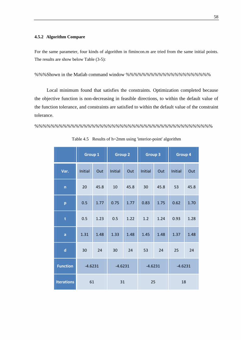
4.5.2 Algorithm Compare
For the same parameter, four kinds of algorithm in fimincon.m are tried from the same initial points.
The results are show below Table (3-5):
%%%Shown in the Matlab command window %%%%%%%%%%%%%%%%%%%%%
Local minimum found that satisfies the constraints. Optimization completed because
the objective function is non-decreasing in feasible directions, to within the default value of
the function tolerance, and constraints are satisfied to within the default value of the constraint
tolerance.
%%%%%%%%%%%%%%%%%%%%%%%%%%%%%%%%%%%%%%%%%%%%
Table 4.5 Results of h=2mm using 'interior-point' algorithm
Group 1 Group 2 Group 3 Group 4
Var. Initial Out Initial Out Initial Out Initial Out
n 20 45.8 10 45.8 30 45.8 53 45.8
p 0.5 1.77 0.75 1.77 0.83 1.75 0.62 1.70
t 0.5 1.23 0.5 1.22 1.2 1.24 0.93 1.28
a 1.31 1.48 1.33 1.48 1.45 1.48 1.37 1.48
d 30 24 30 24 53 24 25 24
Function -4.6231 -4.6231 -4.6231 -4.6231
Iterations 61 31 25 18

59
Table 4.6 Results of h=2mm using 'sqp' algorithm
Group 1 Group 2 Group 3 Group 4
Var. Initial Out Initial Out Initial Out Initial Out
n 20 45.8 10 45.8 30 45.8 53 45.8
p 0.5 2 0.75 1.44 0.83 1.44 0.62 1.71
t 0.5 1.08 0.5 1.50 1.2 1.50 0.93 1.27
a 1.31 1.48 1.33 1.48 1.45 1.48 1.37 1.48
d 30 24 30 24 53 24 25 24
Function -4.6231 -4.6231 -4.6231 -4.6231
Iterations 14 14 11 5
Table 4.7 Results of h=2mm using 'active-set' algorithm
Group 1 Group 2 Group 3 Group 4
Var. Initial Out Initial Out Initial Out Initial Out
n 20 45.8 10 45.8 30 45.8 53 45.8
p 0.5 1.75 0.75 1.44 0.83 1.45 0.62 1.45
t 0.5 1.24 0.5 1.50 1.2 1.50 0.93 1.49
a 1.31 1.48 1.33 1.48 1.45 1.48 1.37 1.48
d 30 24 30 24 53 24 25 24
Function -4.6231 -4.6231 -4.6231 -4.6231
Iterations 19 15 12 8

60
'trust-region-reflective'
The following results would show on the screen:
―Warning: The default trust-region-reflective algorithm does not solve problems with the constraints
you have specified. FMINCON will use the active-set algorithm instead.‖ This means that 'trust-
region-reflective' failed.
Table 4.8 Results compare for different algorithm
Algorithm Initial point x1 x2 x3 x4
'interior-point' Iterations 61 31 25 18
'sqp' 14 14 11 5
'active-set' 19 15 12 8
Compare the results above, from different initial points and through different optimization algorithm,
the output of variables of p and t are different while both the other output variables and final optimized
value function are the same. This is because for different initial guesses, the constraint g2 is active
leading to the product of p and t is constant. t the same time, the function is affected by ―p×t‖ by
coincidence. So the value of function does not change. Furthermore, the total number for iterations in
'sqp' is the least among the algorithm. Thus, the algorithm 'sqp' is selected to complete the following
parametric studies.
Corresponding to baseline [ 40 1.8 1.2 1.4 30]T
, function value f0= -3.5. Improvement is defined by
|f1- f0/f0|
Table 4.9 Results compare for improvement
Group 1 Group 2 Group 3 Group 4
Element Initial Out Initial Out Initial Out Initial Out
Function value f1 -4.6 -4.6 -4.6 -4.6
Improvement 30% 30% 30% 30%

61
4.5.3 Parametric Studies
Table 4.10 Results of h=2.5mm, F=25 kN using 'sqp' algorithm
Group 1 Group 2 Group 3 Group 4
Var. Initial Out Initial Out Initial Out Initial Out
n 20 45.8 10 45.8 30 45.8 53 45.8
p 0.5 1.95 0.75 2 0.83 1.52 0.62 1.47
t 0.5 1.11 0.5 1.08 1.2 1.42 0.93 1.48
a 1.31 1.48 1.33 1.48 1.45 1.48 1.37 1.48
d 30 24 30 24 53 24 25 24
Fval -3.70 -3.70 -3.70 -3.70
Iterations 14 13 12 5
Table 4.11 Results of h=2.2mm, F=30 kN using 'sqp' algorithm 'sqp'
Group 1 Group 2 Group 3 Group 4
Var. Initial Out Initial Out Initial Out Initial Out
n 20 45.8 10 45.8 30 45.8 53 45.8
p 0.5 1.53 0.75 1.80 0.83 1.65 0.62 1.45
t 0.5 1.41 0.5 1.20 1.2 1.32 0.93 1.49
a 1.31 1.48 1.33 1.48 1.45 1.48 1.37 1.48
d 30 24 30 24 53 24 25 24
Fval -3.0758 -3.0758 -3.0758 -3.0758
Iterations 14 15 13 5

62
From the table above, it can be found that the optimized objective function value changed with
different parameters of thickness and force. In addition, for the same input initial variables, the output
variables of p and t also change with different parameters. Finally, the iterations vary a little with
different parameters for the same input initial guess for variables.
When the function is optimized, the variable d reach the low boundary, while the variable a reach the
upper boundary. Also, the other variables n, p, t are the interior solution. From the table, it can be
found that g2, g3, g9 and g12 are active. This result agrees with the monotonicity analysis that g3 is
active.
4.5.4 Discussion of results
The link between this subsystem and the other subsystems are shown below:
Figure 1.15 Interaction between Laser welding optimization and other subsystems
It is possible that the ideal h and d for design optimization and optimization of stamping process can
not been processed by laser welding. Or there is high possibility that acceptable beam power and
exposure time would cause high cost for optimization of manufacturing system, which causes
conflicts. Thus, it is admirable to construct tradeoff between these subsystems.
Some basic rule to optimize laser welding process can be summarized below:
The distance between two neighboring spot welds d should get the value in its low boundary.
The total spot welds per side n can be obtained by transforming the active geometry constraint
g3 into equality.
The incident angle a should be chosen as its upper boundary.
The beam power or exposure time is constrained by the heat input constraint.

63
5 COST OPTIMIZATION OF B-PILLAR PRODUCTION
5.1 Problem Statement
With the rapid development of automotive industry, market competition becomes more and more
serious. Vehicle companies need to reduce products costs, improving products quality and shorten
manufacturing time. The general determining factors in deciding on vehicle production process is
usually cost, that is, to choose a process that produces the required quality at the relatively lowest
possible cost. In this part, we focus on cost reducing of the vehicle B-pillars in order to occupy more
market share. It means that the objective of this subsystem is to minimize the cost of producing B-
pillar.
Production is a vital aspect to decrease the cost in the whole designing, manufacturing and assembly
process. Producing B-pillar mainly contains two processes which are stamping and laser welding. The
costs of this process are specific to some elements of the work. Traditionally, these costs are regarded
as consisting of those for labor, operating and machine. Therefore optimization of labor cost, operating
cost, equipment cost and so on can improve productivity and reduce cost.
Figure 5.1 Automotive manufacturing system

64
5.2 Nomenclature
In this section, we present some parameters and variables, those are used to mathematics
model.
5.2.1 Parameters:
Table 5.1 Parameters
Raw material length of B-pillar 1075mm
Raw material width of B-pillar 340mm
Punch length 1100mm
Punch width 160mm
Punch thickness 70mm
Die length 1100mm
Die width 340mm
Die thickness 70mm
Blank holder length 1100mm
Blank holder width 60mm
Blank holder thickness 20mm
Punch material (Carbon tool steel) cost $900/ton
Die material (Carbon tool steel) cost $900/ton
Blank holder material (Carbon tool steel) cost $900/ton
B-pillar raw material (High strength steel) cost $900/ton
Labor hourly cost $15/ hour
Welding machine cost $10,000
Welding machine lifetime 9 years

65
Hot stamping machine cost $50,000
Hot stamping machine lifetime 10 years
Hot stamping machine power 39 kW
Heating furnace cost $15,200
Heating furnace lifetime 10 years
Heating furnace power 500 kW
Robotics cost $22,000
Robotics lifetime 10 years
Robotics power 3 kW
Hot stamping cooling speed 20s/ available steel plate
Working time each year 360 days
Working time each day 24 hours
Electric charge [10] $0.073/kWh
Density of steel
Die lifetime [11] 11000 times
Total number of spot weld per side 45
Argon cost [12] $0.1/L
Argon usage 5L/min
Absorption coefficient 0.693
Maximum power of spot laser welding machine 2.0kW
Minimum power of spot laser welding machine 0.5kW
Maximum one spot laser welding time 1.5s
Minimum one spot laser welding time 0.5s
Maximum strokes per minute of stamping machine 25 strokes/min

66
Minimum strokes per minute of stamping machine 0
Maximum energy of spot laser welding machine 1.5kJ
Maximum height of B-pillar 45mm
Minimum height of B-pillar 35mm
Maximum raw material thickness of B-pillar 3.0mm
Minimum raw material thickness of B-pillar 1.0mm
5.2.2 Variables
Table 5.2 Variables
SPM Strokes per minute of stamping machine(strokes/min)
h Height of B-pillar(mm)
P Welding power (kW)
t Beam exposure time (s)
H Raw material thickness of B-pillar(mm)

67
5.3 Mathematical Model
Designers typically use some models and simulation tools to finish functional analysis of the design.
According to the current production, we can build a model to simplify the optimization problem.
We simplified the manufacturing system model as dedicated line, that is, there are one Welding
machine and one stamping machine manufacturing. In this manufacturing line, there are some B-
pillars being produced. The model is not to produce a specific production schedule for each of the
individual machines in the machine group. Rather, it is intended to offer a realistic functional form for
the manufacturing costs that are used in the objective function.
The specific steps to optimize cost are as follows. Firstly, I build a model to optimize the production
process in spite of other designing and manufacturing optimization such as welding and stamping
optimization. Secondly, I take parameters and results of other optimization into account to adjust the
optimization result of this part. Thirdly, we can obtain a relatively better whole designing,
manufacturing and assembly optimization result of B-pillar via receiving information, having feedback
to each other and changing some parameters.
5.3.1 Constraints
At first, we choose one kind of spot laser welding machine, its power range is from 0.5kW to 2kW, so
the constraint for the power is given by:
P and
That is and (Equation 5.1)
This time of this machine which finish one spot laser weld is from 0.5s to 1.5s, so the
constraint for the spot welding time is given by:
t and (Equation 5.2)
That is, and (Equation 5.3)

68
We choose one kind of stamping machine, its strokes per minutes can adjust from 0 to 25, so
the constraint f or the stroke time is given by:
and
That is, and (Equation 5.4)
The absorption coefficient is 69.3% of the spot laser welding machine, the maximum energy
of the welding system is 1.5KJ, so the constraint for the energy is given by:
* Pt
That is, 0.693 * Pt (Equation 5.5)
The stamping is ahead of laser welding, the production rate of stamping must be higher than
the production rate of laser welding, otherwise, the dedicated line will bring the blockage. So
the constraint for production rate is given by:
60/(t* )/2 SPM/2
That is, 60/(t*45)/2-SPM/2 (Equation 5.6)
According to the reality, the range of height of B-pillar is always from 35mm to 45mm in the
engineering. So the constraint for height of B-pillar is given by:
and
That is, (Equation 5.7)
According to the reality, the range of raw material thickness of B-pillar is always from 1.0mm
to 3.0mm in the engineering. So the constraint for raw material thickness of B-pillar is given
by:

69
and
That is, (Equation 5.8)
The cooling is ahead of hot stamping. After the raw material heated in the heating furnace, the
material would be cooled and then go to the hot stamping. The production rate of cooling
must be higher than the production rate of hot stamping, otherwise, the dedicated line will
bring the blockage. So the constraint for production rate is given by:
That is, (Equation 5.9)
5.3.2 Modeling
B-pillar production mainly includes two processes which are hot stamping and spot laser welding. The
total cost in the manufacturing contains raw material cost, hot stamping cost and spot laser welding
cost.
Figure 5.2 The component of total cost

70
5.3.2.1 The cost in the stamping process,
The stamping cost includes machine cost, electrical cost, labor cost, die cost, heating furnace cost,
robotics cost.
Figure 5.3 The component of stamping cost
One stroke of the stamping machine forms an available steel plate, two pieces of available
steel plate constitute a B-pillar.
Machine cost = 2* Hot stamping machine cost / Hot stamping machine lifetime / Working
time each year/ Working time each day/ 60minutes/ Strokes per minute of stamping machine =
2* 2 50,000/ 10 / 360 / 24 / 60 / SPM=
/ B-pillar
(Equation 5.10)
Electrical cost = 2* Hot stamping machine power * Electric charge/ 60 minutes/
SPM+2*Heating furnace power* Electric charge/ 60 minutes/ SPM +2*4* Robotics power *
Electric charge/ 60 minutes/ Strokes per minute of stamping machine = =2 / 60 / SPM +
/ 60 / SPM + 2 / 60 / SPM =
B-pillar
(Equation 5.11)
Stamping
Cost
Machine cost
Electrical cost
Labor cost
Die cost
Robotics cost
Heating furnace
cost

71
Labor cost = 2*2* Labor hourly cost/ 60 minutes/ Strokes per minute of stamping machine =
= 2 15 / 60 / SPM=
/ B-pillar (Equation 5.12)
Die cost = 2*[2* Blank holder length* Blank holder width* Blank holder thickness* Density
of steel* ton/kg *Blank holder material (Carbon tool steel) cost + Die length * Die width
*Die thickness*Density of steel* ton/kg *Die material (Carbon tool steel) cost +Punch
length*Punch width*(70- Height of B-pillar) *Density of steel* ton/kg *Punch material
(Carbon tool steel) cost] / Die lifetime = ton/kg ton/kg ton/kg ]/
= = $[0.036+2.26 / B-pillar
(Equation 5.13)
Heating furnace cost=2* Heating furnace cost/ Heating furnace lifetime/ Working time each
year/ Working time each day/ 60minutes/ Strokes per minute of stamping machine =2
= 2 15,200/ 10 / 360 / 24 / 60 / SPM=
/ B-pillar
(Equation 5.14)
Robotics cost=2*4* Robotics cost / Robotics lifetime/ Working time each year/ Working time
each day/ 60minutes/ Strokes per minute of stamping machine =
= 2 22,000/ 10 / 360 / 24 / 60 / SPM=
/ B-pillar
(Equation 5.15)
5.3.2.2 The cost in the welding process
The spot laser welding cost includes machine cost, electrical cost, labor cost, argon cost, robotics cost.
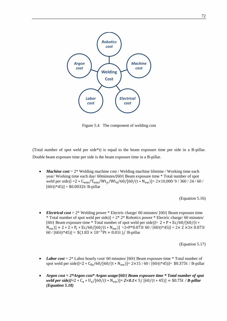
72
Figure 5.4 The component of welding cost
(Total number of spot weld per side*t) is equal to the beam exposure time per side in a B-pillar.
Double beam exposure time per side is the beam exposure time in a B-pillar.
Machine cost = 2* Welding machine cost / Welding machine lifetime / Working time each
year/ Working time each day/ 60minutes/[60/( Beam exposure time * Total number of spot
weld per side)] = = 2 10,000/ 9 / 360 / 24 / 60 /
[60/(t*45)] = / B-pillar
(Equation 5.16)
Electrical cost = 2* Welding power * Electric charge/ 60 minutes/ [60/( Beam exposure time
* Total number of spot weld per side)] + 2* 2* Robotics power * Electric charge/ 60 minutes/
[60/( Beam exposure time * Total number of spot weld per side)]= =2 P* / 60 / [60/(t*45)] + 2 3 /
60 / [60/(t*45)] = B-pillar
(Equation 5.17)
Labor cost = 2* Labor hourly cost/ 60 minutes/ [60/( Beam exposure time * Total number of
spot weld per side)]= = 2 15 / 60 / [60/(t*45)]= / B-pillar
Argon cost = 2*Argon cost* Argon usage/[60/( Beam exposure time * Total number of spot
weld per side)]= = 2 0.1 / B-pillar
(Equation 5.18)
Welding
Cost
Robotics cost
Machine cost
Electrical cost
Labor cost
Argon cost

73
Robotics cost=2*2* Robotics cost / Robotics lifetime/ Working time each year/ Working time
each day/ 60minutes/ [60/( Beam exposure time * Total number of spot weld per side)]= = 2 $22,000/ 10 years/ 360 days/ 24 hours/ 60
minutes/ [60/(t*45)]= / B-pillar
(Equation 5.20)
5.3.2.3 Material cost
Material cost =2* Raw material length of B-pillar * Raw material width of B-pillar * Raw
material thickness of B-pillar * Density of steel* Raw material (High strength steel) cost of B-
pillar =
=
/B-pillar
(Equation 5.21)
5.3.2.4 Model Sumary
Min f = Machine cost in the stamping process + Electrical cost in the stamping process + Labor cost
in the stamping process + Die cost in the stamping process + Heating furnace cost in the stamping
process Robotics cost in the stamping process + Machine cost in the welding process+ Electrical
cost in the welding process + Labor cost in the welding process + Argon cost in the welding process
+ Robotics cost in the welding process + Material cost
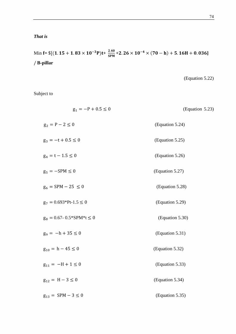
74
That is
Min f= 𝟓 𝟖𝟑 𝟑 + 𝟐 𝟒
+𝟐 𝟐𝟔 𝟒 𝟕 𝟓 𝟔 𝟑𝟔]
B-pillar
(Equation 5.22)
Subject to
(Equation 5.23)
2 (Equation 5.24)
(Equation 5.25)
(Equation 5.26)
(Equation 5.27)
(Equation 5.28)
0.693*Pt-1.5 (Equation 5.29)
0.67- 0.5*SPM*t (Equation 5.30)
(Equation 5.31)
(Equation 5.32)
(Equation 5.33)
2 (Equation 5.34)
(Equation 5.35)

75
5.4 Optimization Model Analysis
5.4.1 Monotonicity Analysis
A monotonicity analysis with respect to the design variables are performed for checking whether the
problem is well constrained. The monotonicities of all the variables with respect to the objective
function and constraints are shown in the table below.
Table 4 Monotonicity Analysis
SPM h P t H
f - - + + +
- Active for variable P
2 +
- Active for variable t
+
-
+
+ +
- -
-
+ Active for variable h
- Active for variable H
2 +
+ Active for variable SPM
76
When other variables are fixed, and only SPM can change. Objective function decreases in a variable
SPM. Constraint and Constraint increase in a variable SPM.
, 0, so
When other variables are fixed, and only h can change. Objective function decreases in a variable h.
Constraint increases in a variable h. , so
When other variables are fixed, and only P can change. Objective function increases in a variable P.
Constraint decreases in a variable h. , so
When other variables are fixed, and only t can change. Objective function increases in a variable t.
Constraint and Constraint decrease in a variable t. 0.67-
0.5*SPM*t , when SPM is from 0 to 3, and can not be judged the relationship, so
When other variables are fixed, and only H can change. Objective function increases in a variable H.
Constraint decreases in a variable H. , so

77
5.5 Numerical Optimization
%Shown in Matlab command window%%%%%%%%%%%%%%%%%%%%%%%%%%
Local minimum possible. Constraints satisfied.
fmincon stopped because the predicted change in the objective function is less than the default
value of the function tolerance and constraints are satisfied to within the default value of the
constraint tolerance.
<stopping criteria details>
Active inequalities (to within options.TolCon = 1e-006):
lower upper ineqlin ineqnonlin
1 3 2
2
5
%%%%%%%%%%%%%%%%%%%%%%%%%%%%%%%%%%%%%%%%%
There are four algorithms in fmincon.m. I used one of algorithm, that is, 'interior-point' algorithm. I
tried this algorithm from different initial points. The results are shown below:

78
Table 5.5 Optimization results for various starting points
Test 1 Test 2 Test 3 Test 4
Var. Initial Out Initial Out Initial Out Initial Out
p 0.5 0.5002 0.9 0.5024 0.65 0.5001 1.2 0.5004
t 0.5 0.5 1.3 0.5 0.75 0.5 0.6 0.5
SPM 1 3 2 3 1 3 3 3
h 35 44.9996 45 44.9902 37 44.9996 40 44.9982
H 1 1 2 1 3 1 3 1
Fval 8.1794 6.5771 7.8988 6.5771 18.7869 6.5771 17.0141 6.5771
Iterations 24 19 24 21
From the results above, the 'interior-point' algorithm, we can get the local minimum which is
$6.5771/B-pillar. From the initial points and out points in different situations, we can obtain
improvement over starting points. Then, different parameters are tried to optimize the function again.
From the table below, it can be found that the function value changed for different parameters while
the iteration does not change too much.

79
Table 5.6 Results of 'interior-point' algorithm using n=30
Test 1 Test 2 Test 3 Test 4
Var. Initial Out Initial Out Initial Out Initial Out
p 0.5 0.5002 0.9 0.5024 0.65 0.5001 1.2 0.5004
t 0.5 0.5 1.3 0.5 0.75 0.5 0.6 0.5
SPM 1 3 2 3 1 3 3 3
h 35 44.9996 45 44.9902 37 44.9996 40 44.9982
H 1 1 2 1 3 1 3 1
Fval 6.4756 6.4756 6.4756 6.4756
Iterations 23 19 23 22
Table 5.7 Results of 'interior-point' algorithm using n=40
Test 1 Test 2 Test 3 Test 4
Var. Initial Out Initial Out Initial Out Initial Out
p 0.5 0.5002 0.9 0.5024 0.65 0.5001 1.2 0.5004
t 0.5 0.5 1.3 0.5 0.75 0.5 0.6 0.5
SPM 1 3 2 3 1 3 3 3
h 35 44.9996 45 44.9902 37 44.9996 40 44.9982
H 1 1 2 1 3 1 3 1
Fval 6.5233 6.5233 6.5233 6.5233
Iterations 24 19 23 21
From the table above, we can find when we change the total number of spot weld per side
from 45 to 30 and 40, the local minimum will decrease. It means that the cost which produces
one B-pillar will decrease. And the iteration does not change too much.

80
5.6 Discussion of Results
From the parameters study results, the lowest cost of manufacturing is obtained when the
beam power, stamping height and exposure time reach their lower boundary while the SPM
and the thickness of plate get their values on upper boundary. It makes sense that when beam
power and exposure time decrease, energy cost for laser welding reduces. The productivity
would increase with stamping height decreasing and SPM increasing. Thus the cost of
manufacturing process is the lowest at the above minimizer just for this subsystem.
Figure 5.5 Relation between manufacturing subsystem and the other subsystems
The low cost requirement of manufacturing subsystem optimization required that small geometry for
design, high speed for stamping process, and low power and exposure time for laser welding. While
these requirement maybe cause trouble in other subsystem. So, tradeoff is needed to construct the
complete project.
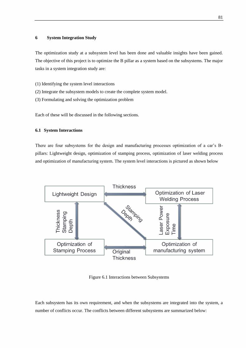
81
6 System Integration Study
The optimization study at a subsystem level has been done and valuable insights have been gained.
The objective of this project is to optimize the B pillar as a system based on the subsystems. The major
tasks in a system integration study are:
(1) Identifying the system level interactions
(2) Integrate the subsystem models to create the complete system model.
(3) Formulating and solving the optimization problem
Each of these will be discussed in the following sections.
6.1 System Interactions
There are four subsystems for the design and manufacturing processes optimization of a car‘s B-
pillars: Lightweight design, optimization of stamping process, optimization of laser welding process
and optimization of manufacturing system. The system level interactions is pictured as shown below
Figure 6.1 Interactions between Subsystems
Each subsystem has its own requirement, and when the subsystems are integrated into the system, a
number of conflicts occur. The conflicts between different subsystems are summarized below:

82
Table 8.1 Conflicts between different subsystems
6.2 Problem Formulation
Once the subsystem models are integrated, the optimization problem for the complete system has to be
defined. There are two objectives for the system: one is to reduce the cost to build lightweight B-pillar
structure, and the other is to reduce the structure weight. This is multiobjective problem. The ultimate
objective function can be obtained by assigning subjective weights to each objective and summing up
these two objectives multiplied by their corresponding weight.
The overall system problem can be formulated as follows
ℎ 2 ℎ
Subjected to the following two kinds of constraints:
Total mass
Peak acceleration
Maximum intrusion
Spot-welding safety factor
Spot-welding quality

83
Stamping punch force
Stamping elongation
Manufacturing cost
Spot-welding geometry
The specific constraints are shown as Matlab code in the appendix.
Final Set of variables are summarized as
Table 6.1 Variables summary
Description Symbol
laser power p
exposure time during laser spot-welding T
frequency of stamping SPM
stamping depth h
thickness of raw steel panel t0
thickness of lower component panel t1
thickness of upper component panel t2

84
Objects of other subsystem problems now become the constraint function after reference object values
are defined as the design boundary, which are shown in following table. Besides, the system
problem also subject to those constraints functions that subsystems already have.
Table 6.2 Constraints functions summary
Total mass ∑
Peak acceleration ℎ
Maximum intrusion ℎ
Spot-welding safety factor
2
Spot-welding quality
2
Stamping quality ℎ 2 ℎ ,
where
6.3 Optimization Approaches
In the system level, Matlab function: fmincon is still applied to find out the optimum solution. 5 times
of running are conducted, no solution is obtained. The fmincon reports no feasible design space with
all these constraints provided. Then the design space is enlarged by loose the bounds, and another 5
rounds are tried. Only one solution is obtained, which is shown as follows:
Table 6.3 Optimization result summary
Description Initial Output
laser power 0.7 1.6
exposure time 1.3 0.7
frequency of stamping 1.6 2.6
ℎ stamping depth 44 48
thickness of raw steel panel 1.9 1.0
thickness of lower component panel 1.6 1.0
thickness of upper component panel 2.3 1.0
Function value 5.2 2.9
Improvement 44%
Iteration 94

85
From the result we can tell that although the improvement of object function is significant, some of the
design variables in this result already exceed over the initial feasible area, like ℎ, the stamping depth
which is initially defined between 35-45mm . This means the variables are chosen from the design area
that metamodel has no real information but only regression trend, thus the result is quite suspicious for
their ability to reflect the real situation. The validation of this result needs experiments in real scenario,
which are only accessible for subsystem 1 in our problem, and its result, though shows good match,
cannot be enough to prove the whole result for system optimization.
6.4 Dicussion
The system integration in optimization problems is always a very challenging task. To ensure that the
design space of each subsystem can overlap with others, expert knowledge in not just sub disciplines
but also system level is required to well define the problem before optimization. Besides, there are 4
nonlinear constraints in our system level problem that use non-analytical model to simulate the real
result, which may cause significant discontinuity of the final design space, and make the optimization
algorithm difficult to converge. Heuristic method may be needed to deal with such situation. And
again, a efficient heuristic method still requires expert knowledge to reduce the ―guessing‖ time to
initial the optimization iteration.

86
7 REFERENCES
[1] Pan, F., Zhu, P., & Zhang, Y. (2010). Metamodel-based lightweight design of B-pillar with TWB
structure via support vector regression. Computers & Structures, 88(1-2), 36-44. Elsevier Ltd.
doi:10.1016/j.compstruc.2009.07.008
[2] Qin Y., Kong X., & Luo, W. (2011). Finite element model updating of airplane wing based on
Gaussian radial bassis function response surface. Jounral of Beijing University of Aeronautics
and Astronautics, 37(11), 1465-1470. 2011.11
[3] Firat, Mehmet, Osman H. Mete, Umit Kocabicak, and Murat Ozsoy. "Stamping Process Design
Using FEA in Conjunction with Orthogonal Regression." Finite Elements in Analysis and Design
46.11 (2010): 992-1000.
[4] Z. Marchiniak, J.L.Duncan, S.J.Hu, ―Mechanics of Sheet Metal Forming‖, 2002;
[5] Peng, L., P. Hu, X. Lai, D. Mei, and J. Ni. "Investigation of Micro/meso Sheet Soft Punch
Stamping Process – Simulation and Experiments." Materials & Design 30.3 (2009): 783-90.
[6] http://www.seas.virginia.edu/research/lam/pdfs/speaker%20presentations/Havrilla-
UofV_Laser%20Based%20Manufacturing%20in%20the%20Automotive%20Industry.pdf
[7] C.M. Sonsino, M. Kueppers, M. Eibl, G. Zhang, Fatigue strength of laser beam welded thin steel
structures under multiaxial loading, International Journal of Fatigue, Volume 28, Issues 5–6,
May–June 2006, Pages 657-662.
[8] Y.S. Yang, S.H. Lee, A study on the joining strength of laser spot welding for automotive
applications, Journal of Materials Processing Technology, Volume 94, Issues 2–3, 29 September
1999, Pages 151-156.
[9] Q. Huang, J. Hagstroem, H. Skoog, G. Kullberg, Effect of laser parameter variation on sheet
metal welding, Int. J. Join. Mater. 3 (3) (1991) 79–88.
[10] Minggang, ji et al., Design of Machinery, Higher Education Press, 2006
[11] Phillips, Arthur L ,, and American Welding Society.,. Welding Handbook. New York,
1957.
[12] Siva Shanmugam, N., G. Buvanashekaran, and K. Sankaranarayanasamy. "Some Studies on Weld
Bead Geometries for Laser Spot Welding Process Using Finite Element Analysis." Materials

87
& Design 34 (2012): 412-26.
[13] Aderoba, A., A generalized cost-estimation model for job shops. International Journal of
Production Econonomics, 1997
[14] http://www.net114.com/100376571p.html
[15] http://www.net114.com/101148101p.html
[16] http://zhidao.baidu.com/question/108800894.html
[17] http://www.alibaba.com/showroom/laser-welding-machine-price.html
[18] http://www.wjw.cn/product/MBR110226095213734898/PRO110411033834609919.xhtml
[19] http://www.machine35.com/product/trade/2-13.html
[20] http://zhidao.baidu.com/question/179273445.html
[21] http://www.jdzj.com/products/2011-8-4/7509176-1.html
[22] http://blog.sina.com.cn/s/blog_62f5246d0100m7af.html
[23] http://wenku.baidu.com/view/d20623e3524de518964b7dd8.html
[24] http://www.hilarion.com/igd.html
[25] http://wenku.baidu.com/view/83040809bb68a98271fefaf9.html
[26] http://woodhead.metapress.com
[27] http://www.alibaba.com/product-gs/518148409/press_used_metal_heating_furnace.html
[28] http://www.alibaba.com/product-gs/472508927/High_speed_Running_AMD_255_series.html

88
8 Apprendix
8.1 MATLAB Code for the structure optimization
% ===========================================================
% NeuralTrain is to train radical based neural network
% ===========================================================
function[net] = NeuralTrain(p)
% X = n x q matrix of q vectors with n dimensional continuous variables
% read training set from DoE spreadsheet
p = 4;
X0_in = csvread('DoE_sheet.csv');
% transpose the DoE matrix, for that the spreadsheet is in q x n formation
X0 = X0_in(1:25*p,:)';
% normalize design variables
lgt = size(X0,2);
h_0 = 35.0 * ones(1,lgt);
89
t1_0 = 1.0 * ones(1,lgt);
t2_0 = 1.0 * ones(1,lgt);
v_lower = 0.2 * ones(1,lgt);
% normalize training set
% X0_Norm(1,:) = v_lower + 0.6 * (X0(1,:) - h_0)/10;
% X0_Norm(2,:) = v_lower + 0.6 * (X0(2,:) - t1_0)/1.4;
% X0_Norm(3,:) = v_lower + 0.6 * (X0(3,:) - t2_0)/1.4;
% X_0 = X0_Norm;
X_0 = X0;
% read the FE simulation result of training set
D_0 = csvread('Intrusion.csv');
A_0 = csvread('Acceleration.csv');
q = numel(D_0);
Con_0 = zeros(2,q);
90
for i = 1:q
intr = D_0(i);
acc = A_0(i);
Con_0(:,i) = [intr,acc]';
end
size(Con_0);
size(X_0);
[onet tr] = newrb(X_0,Con_0,0.01,1.5,50,5);
% X_0 = n x q matrix of q normalized input vectors
% Con_0 = s x q matrix of q constraint value vectors
% mean squared error goal = 0.01
% spread of radial basis function = 2.5
% maximum num of neurons = 50
save metamodel.mat onet;
end

91
% ===========================================================
% Metafun is to generate the metamodel based on neural network
% ===========================================================
function[Con_X] = Metafun(X)
% X = n x q matrix of q vectors with n dimensional continuous variables
% normalize design variables
lgt = size(X,2);
h_0 = 35.0 * ones(1,lgt);
t1_0 = 1.0 * ones(1,lgt);
t2_0 = 1.0 * ones(1,lgt);
v_lower = 0.2*ones(lgt,1);
% normalize testing set
% X_Norm(1,:) = v_lower + 0.6 * (X(1,:) - h_0)/10;
% X_Norm(2,:) = v_lower + 0.6 * (X(1,:) - t1_0)/1.4;
% X_Norm(3,:) = v_lower + 0.6 * (X(1,:) - t2_0)/1.4;

92
% X_1 = X_Norm;
X_1 = X;
% load the neural network trained by traing set.
load metamodel.mat;
q = size(X,2);
Con_X = zeros(2,q);
for i = 1:q
Con_X(:,i) = sim(onet,X_1(:,i));
end
end
% ===========================================================
% Visualization provides the 3-D scatters for monotonicity study
% ===========================================================
X_1 = csvread('DoE_sheet.csv');

93
x1 = X_1(:,1);
x2 = X_1(:,2);
x3 = X_1(:,3);
n = 25;
xx1 = linspace(min(x1),max(x1),n);
xx2 = linspace(min(x2),max(x2),n);
xx3 = linspace(min(x3),max(x3),n);
[X1,X2,X3] = meshgrid(xx1,xx2,xx3);
H = reshape (X1,[n^3,1]);
Tl = reshape (X2,[n^3,1]);
Tu = reshape (X3,[n^3,1]);
%X = [35,1.4,1.4;40,1.2,1.6;44,1.1,1.7];
X = [H,Tl,Tu];
for i = 1:size(X,1)

94
[C] = Metafun(X(i,:)');
Mass(i,1) = Wgt(X(i,:)');
Intr(i,1) = C(1);
Acc(i,1) = C(2);
end
Mass3 = reshape (Mass,[n,n,n]);
Intr3 = reshape (Intr,[n,n,n]);
Acc3 = reshape (Acc ,[n,n,n]);
hmodel = scatter3(X1(:),X2(:),X3(:),5,Mass3(:),'filled');
hold on
hdata = scatter3(x1,x2,x3,'ko','filled');
axis tight
xlabel(xn(1,:))
ylabel(xn(2,:))
95
zlabel(xn(3,:))
hbar = colorbar;
ylabel(hbar,yn);
title('{\bf Quadratic Response Surface Model}')
legend(hdata,'Data','Location','NE')
% ===========================================================
% LatinDoE is to generate the initial points for optimization
% ===========================================================
function [D_1] = LatinDoE(i,j)
X = lhsdesign(i,j);
% i levels
% j variables
h = 35+10*X(:,1);
t_l = 1.0+1.4*X(:,2);
t_2 = 1.0+1.4*X(:,3);

96
D_1 = [h,t_l,t_2]';
end
% ===========================================================
% mycon defines the nonlinear constraints of optimization problem
% ===========================================================
function [c,ceq] = mycon(x)
[Con] = Metafun(x);
Intr = Con(1);
Acc = Con(2);
% baseline model: t1 = 1.8, t2 = 2.4, h = 40;
IntrBaseline = 70.0000;
AccBaseline = 5.5000;
c(1) = Intr - IntrBaseline ;
c(2) = Acc - AccBaseline;

97
c(3) = 50 - Intr;
c(4) = 3 - Acc;
ceq = [];
end
% ===========================================================
% Wgt defines the object of lightweight design
% ===========================================================
function [w] = Wgt(X)
% X = n * 1 , the vector of n dimensional continuous variables
l = [3.750E-04, 3.887e-04, 4.026e-04];
u = [1.233E-03, 1.278e-03, 1.324e-03];
h = [35,40,45];
c_1 = (l(2)-l(1))/(h(2)-h(1));

98
c_2 = (l(3)-l(2))/(h(3)-h(2));
c_3 = (l(3)-l(1))/(h(3)-h(1));
c_l = (c_1+c_2+c_3)/3;
c_4 = (u(2)-u(1))/(h(2)-h(1));
c_5 = (u(3)-u(2))/(h(3)-h(2));
c_6 = (u(3)-u(1))/(h(3)-h(1));
c_u = (c_4+c_5+c_6)/3;
h_r = X(1,1);
t_1 = X(2,1);
t_2 = X(3,1);
w_l = (c_l*(h_r-35)+3.750E-04) * t_1;
w_u = (c_u*(h_r-35)+1.233E-03) * t_2;
w = w_l + w_u;
end

99
% ===========================================================
% OptimizeFun uses the fmincon to find the optimal solution
% ===========================================================
function [] = OptimizeFun()
A = [];
b = [];
Aeq = []; beq = [];
lb = [35;1.0;1.0];
ub = [45;2.4;2.4];
X = cell(5,1);
x_Star = cell(5,6);
for i = 1:5
n = 3;
q = 6;

100
x = LatinDoE(q,n);
X{i,1} = x;
for j = 1:q
x0 = x(:,q);
[xval,fval,exitflag,output] = fmincon(@Wgt,x0,A,b,Aeq,beq,lb,ub,@mycon);
Mass_Star(i,j) = fval;
x_Star{i,j} = xval;
Con = Metafun(xval);
Intru_Star(i,j) = Con(1);
Acc_Star(i,j) = Con(2);
Iteration(i,j) = output;
end
end
101
8.2 MATLAB Code for the stamping optimization
DoE
function [D_1] = LatinDoE (n)
% n value levels
p = 4; % p design variables
X = lhsdesign(n,p);
h = 35 + 20*X(:,1);
t = 1.4 + 1.0*X(:,2);
u = 0.05 + 0.73*X(:,3);
F = 85 + 165*X(:,4);
D_1 = [h,t,u,F];
end

102
Scaled objective function
clear all;
M = csvread('vv.csv');
hn=M(:,1);
tn=M(:,2);
un=M(:,3);
Fn=M(:,4);
Fpn=M(:,5);
%normalize
h = 0.1+0.8*(hn - min(hn)*ones(size(hn,1),1))/(max(hn)-min(hn));
t = 0.1+0.8*(tn - min(tn)*ones(size(tn,1),1))/(max(tn)-min(tn));
u = 0.1+0.8*(un - min(un)*ones(size(un,1),1))/(max(un)-min(un));
F = 0.1+0.8*(Fn - min(Fn)*ones(size(Fn,1),1))/(max(Fn)-min(Fn));
Fp = 0.1+0.8*(Fpn - min(Fpn)*ones(size(Fpn,1),1))/(max(Fpn)-min(Fpn));
x=[h t u F h.^2 t.^2 u.^2 F.^2 (h.*t) (h.*u) (t.*u) (t.*F) (u.*F) (h.*F)];

103
X=[ones(50,1),x];
%stepwise(X,Fp);
XF=[ones(50,1) h t u F h.^2 t.^2 u.^2 F.^2 (h.*t) (h.*u) (t.*u) (t.*F)
(u.*F) (h.*F)];
XF1= [ones(50,1) u F u.^2 (h.*t) (u.*F)];
[b,bint,r,rint,stats]=regress(Fp,XF1);
Constraint function
clear all;
M = csvread('ss.csv');
h=M(:,1);
t=M(:,2);
u=M(:,3);
F=M(:,4);
s=M(:,5);
x=[h t u F h.^2 t.^2 u.^2 F.^2 (h.*t) (h.*u) (t.*u) (t.*F) (u.*F) (h.*F)];

104
X=[ones(50,1),x];
%stepwise(X,s);
XF=[ones(50,1) h t u F h.^2 t.^2 u.^2 F.^2 (h.*t) (h.*u) (t.*u) (t.*F)
(u.*F) (h.*F)];
Xs=[ones(50,1) h t u F h.^2 t.^2 u.^2 F.^2 (h.*t) (h.*u) (t.*u) (t.*F)
(u.*F) (h.*F)];
Xs1= [ones(50,1) h t u F t.*F];
[b,bint,r,rint,stats]=regress(s,Xs1);
Fmincon
function f=objfun(x)
%x = [39.7,2.18,0.53,211.1];
M = csvread('vv.csv');
hn = M(:,1);
tn = M(:,2);
un = M(:,3);
Fn = M(:,4);

105
h = 0.1+0.8*(hn - min(hn)*ones(size(hn,1),1))/(max(hn)-min(hn));
t = 0.1+0.8*(tn - min(tn)*ones(size(tn,1),1))/(max(tn)-min(tn));
u = 0.1+0.8*(un - min(un)*ones(size(un,1),1))/(max(un)-min(un));
F = 0.1+0.8*(Fn - min(Fn)*ones(size(Fn,1),1))/(max(Fn)-min(Fn));
x = [h t u F];
W = csvread('obj.csv');
w_1 = W(:,1);
x_1(1) = 1;
x_1(2,1) = x(1);
x_1(3,1) = x(2);
x_1(4,1) = x(3);
x_1(5,1) = x(4);
x_1(6,1) = x(1)^2;
x_1(7,1) = x(2)^2;
x_1(8,1) = x(3)^2;

106
x_1(9,1) = x(4)^2;
x_1(10:15,1) = [x(1)*x(2);
x(1)*x(3);
x(2)*x(3);
x(2)*x(4);
x(3)*x(4);
x(1)*x(4)];
h_1 = [0 1 0 0 0 0 0 0 0 0 0 0 0 0 0 ];
h_2 = [0 0 1 0 0 0 0 0 0 0 0 0 0 0 0 ];
a = w_1'*x_1;
b = h_1*x_1;
c = h_2*x_1;
f = a-b+c;

107
end
function [c,ceq] = mycon(x)
% x = [h,t,u,F]
%x = [1,2,3,4];
C = csvread('constrain.csv');
c_1 = C(:,1);
x_1(1) = 1;
x_1(2,1) = x(1);
x_1(3,1) = x(2);
x_1(4,1) = x(3);
x_1(5,1) = x(4);
x_1(6,1) = x(1)^2;
x_1(7,1) = x(2)^2;
x_1(8,1) = x(3)^2;
x_1(9,1) = x(4)^2;

108
x_1(10:15,1) = [x(1)*x(2);
x(1)*x(3);
x(2)*x(3);
x(2)*x(4);
x(3)*x(4);
x(1)*x(4)];
c(1) = c_1'* x_1-270;
W = csvread('obj.csv');
w_1 = W(:,1);
c(2) = -w_1'*x_1;
ceq= [];
end
clear all;
x0= [36,1.6,0.64,117.26];

109
lb= [35,1.4,0.05,83.3];
ub= [55,2.4,0.78,250];
options = optimset('Algorithm', 'active-set');
[x,fval,exitflag,output]=
fmincon(@objfun,x0,[],[],[],[],lb,ub,@mycon,options);

110
8.3 MATLAB Code for the welding optimization
Appendix I
Before input the following code, the data ‗Depth‘ has to be uploaded into the Matlab.
Matlab code for regression the function DP:
clc;
clear all;
p=depth(:,1);
t=depth(:,2);
a=depth(:,3);
DP=depth(:,4);
x=[p t a (p.*t) (p.*a) (a.*t) (p.^2) (t.^2) (a.^2)];
X=[ones(27,1),x];
stepwise(X,DP);
X1=[ ones(27,1) p (p.*t) (p.*a) (a.*t) (p.^2)];
[b,bint,r,rint,stats]=regress(DP,X1);
Matlab code for regression the function BW:
clc;

111
clear all;
p=depth(:,1);
t=depth(:,2);
a=depth(:,3);
BW=depth(:,5);
x=[p t a (p.*t) (p.*a) (a.*t) (p.^2) (t.^2) (a.^2)];
X=[ones(27,1),x];
stepwise(X,BW);
Variables have been created in the current workspace.
>> X2=[ones(27,1) a (p.*t)];
[b,bint,r,rint,stats]=regress(BW,X2);

112
Step 1: Write a file objfun.m.
function f=objfun(x)
f=-0.0245*x(1)*((-1.1716+1.4939*x(4)+0.4549*x(2)*x(3))^2);
Step 2: Write a file confuneq.m for the nonlinear constraints.
function [c, ceq]= confun(x)
c = [1.1618+3.3717*x(2)-0.2715*x(2)*x(3)-1.3096*x(2)*x(4)-0.1223*x(4)*x(3)-
1.6284*(x(2)^2);
0.693*x(2)*x(3)-1.5;
(x(1)-1)*x(5)-1075];
ceq = [];
Step 3: Invoke constrained optimization routine.
clc;
clear all;
x0= [20,0.5,0.5,1.31,30]; % Make a starting guess at the solution
lb= [0,0.5,0.5,1.309,24];
ub= [Inf,2,1.5,1.484,70];
options = optimset('Algorithm','active-set');% Line a
[x,fval,exitflag,output]=
fmincon(@objfun,x0,[],[],[],[],lb,ub,@confun,options);

113
For the other fmincon Algorithms, they can be simply done by replace 'active-set' in line
a with 'sqp', 'active-set', 'trust-region-reflective' .
%%%%%%%%%%%%%%%%%%%%%%%%%%%%%%%%%%%%%%%%%%%%
%Optimization h=2.5mm F=25KN
function f=objfun(x)
f=-0.0196*x(1)*((-1.1716+1.4939*x(4)+0.4549*x(2)*x(3))^2);
function [c, ceq]= confun(x)
c = [1.6618+3.3717*x(2)-0.2715*x(2)*x(3)-1.3096*x(2)*x(4)-0.1223*x(4)*x(3)-
1.6284*(x(2)^2);
0.693*x(2)*x(3)-1.5;
(x(1)-1)*x(5)-1075];
ceq = [];
clc;
clear all;
x0= [53,0.62,0.93,1.37,25];

114
%x0= [20,0.5,0.5,1.31,30];
%x0= [10,0.75,0.5,1.33,30];
%x0= [30,0.83,1.2,1.45,53];
lb= [0,0.5,0.5,1.309,24];
ub= [Inf,2,1.5,1.484,70];
options = optimset('Algorithm', 'sqp');
[x,fval,exitflag,output]= fmincon(@objfun,x0,[],[],[],[],lb,ub,@confun,options);
%%%%%%%%%%%%%%%%%%%%%%%%%%%%%%%%%%%%%%%%%%%%
%Optimization h=2.2mm F=30KN
function f=objfun(x)
f=-0.0163*x(1)*((-1.1716+1.4939*x(4)+0.4549*x(2)*x(3))^2);
function [c, ceq]= confun(x)
c = [1.3618+3.3717*x(2)-0.2715*x(2)*x(3)-1.3096*x(2)*x(4)-0.1223*x(4)*x(3)-
1.6284*(x(2)^2);
0.693*x(2)*x(3)-1.5;

115
(x(1)-1)*x(5)-1075];
ceq = [];
clc;
clear all;
x0= [53,0.62,0.93,1.37,25];
%x0= [20,0.5,0.5,1.31,30];
%x0= [10,0.75,0.5,1.33,30];
%x0= [30,0.83,1.2,1.45,53];
lb= [0,0.5,0.5,1.309,24];
ub= [Inf,2,1.5,1.484,70];
options = optimset('Algorithm', 'sqp');
[x,fval,exitflag,output]= fmincon(@objfun,x0,[],[],[],[],lb,ub,@confun,options);

116
8.4 MATLAB Code for the cost optimization
When the number of spot weld =40
Objective function
function f=objfun(x)
f=(1.15+0.00183*x(1))*x(2)+2.4/x(3)+2.26e-4*(70-x(4))+5.16*x(5)+0.036;
Nonlinear constraint
function [c, ceq]= confun(x)
c = [0.693*x(1)*x(2)-1.5;
0.67-0.5*x(2)*x(3)];
ceq = [];
Optimization method
clc;
clear all;
x0= [0.5,0.5,1,35,1];
%x0= [0.65,0.75,1,37,3];
%x0= [0.9,0.13,2,45,2];
%x0= [1.2,0.6,3,40,3];

117
lb= [0.5,0.5,0, 35,1];
ub= [2,1.5,3,45, 3];
options = optimset('Algorithm', 'active-set' );
[x,fval,exitflag,output]= fmincon(@objfun,x0,[],[],[],[],lb,ub,@confun,options);