The Demographics of Innovation and Asset Returns
49
The Demographics of Innovation and Asset Returns Nicolae Garleanu ∗ UC Berkeley, NBER, and CEPR Leonid Kogan † MIT and NBER Stavros Panageas ‡ Univ. of Chicago Booth School of Business and NBER First Draft, July 2008 Current Draft, November 2008 Abstract We study an overlapping-generations economy in which new agents innovate and introduce new products and firms. Innovation is stochastic. The new firms increase overall productivity, but also steal business from pre-existing firms and act as depreci- ation shocks for the human capital of existing agents. Since new firms belong to newly arriving agents, innovations are a double-edged sword for pre-existing generations: In- creased innovation activity increases the total output, but it also reduces the share of the pre-existing agents in the increased output. The latter effect — “the displacement risk” — makes agents reluctant to hold stock in firms whose output is exposed to in- creased innovation and competition by new firms, while giving a hedging value to firms that can profit from innovation. Therefore the model produces a value effect. At the aggregate level the displacement risk makes agents reluctant to hold stock of existing firms, since their profits are collectively at risk from new entrants. This leads to a higher equity premium. We calibrate the model so that it can match estimated cohort effects for individuals and firms, and evaluate its quantitative implications. ∗ Haas School of Business, UC Berkeley, 545 Student Services Building, Berkeley, CA94720-1900, Phone: 510 642 3421, email: [email protected] † Sloan School of Management, MIT, and NBER, E52-434, 50 Memorial Drive, Cambridge, MA 02142, tel: (617)253-2289, e-mail: [email protected] ‡ University of Chicago Booth School of Business, 5807 South Woodlawn Avenue, Office 313, Chicago, IL, 60637, tel: 773 834 4711, email: [email protected] 1
description
We study an overlapping-generations economy in which new agents innovate andintroduce new products and firms. Innovation is stochastic. The new firms increaseoverall productivity, but also steal business from pre-existing firms and act as depreciationshocks for the human capital of existing agents. Since new firms belong to newlyarriving agents, innovations are a double-edged sword for pre-existing generations: Increasedinnovation activity increases the total output, but it also reduces the share ofthe pre-existing agents in the increased output. The latter effect — “the displacementrisk” — makes agents reluctant to hold stock in firms whose output is exposed to increasedinnovation and competition by new firms, while giving a hedging value to firmsthat can profit from innovation. Therefore the model produces a value effect. At theaggregate level the displacement risk makes agents reluctant to hold stock of existingfirms, since their profits are collectively at risk from new entrants. This leads to ahigher equity premium. We calibrate the model so that it can match estimated cohorteffects for individuals and firms, and evaluate its quantitative implications.
Transcript of The Demographics of Innovation and Asset Returns

The Demographics of Innovation and Asset Returns
Nicolae Garleanu∗
UC Berkeley, NBER, and CEPRLeonid Kogan†
MIT and NBER
Stavros Panageas‡
Univ. of Chicago Booth School of Business and NBER
First Draft, July 2008
Current Draft, November 2008
Abstract
We study an overlapping-generations economy in which new agents innovate andintroduce new products and firms. Innovation is stochastic. The new firms increaseoverall productivity, but also steal business from pre-existing firms and act as depreci-ation shocks for the human capital of existing agents. Since new firms belong to newlyarriving agents, innovations are a double-edged sword for pre-existing generations: In-creased innovation activity increases the total output, but it also reduces the share ofthe pre-existing agents in the increased output. The latter effect — “the displacementrisk” — makes agents reluctant to hold stock in firms whose output is exposed to in-creased innovation and competition by new firms, while giving a hedging value to firmsthat can profit from innovation. Therefore the model produces a value effect. At theaggregate level the displacement risk makes agents reluctant to hold stock of existingfirms, since their profits are collectively at risk from new entrants. This leads to ahigher equity premium. We calibrate the model so that it can match estimated cohorteffects for individuals and firms, and evaluate its quantitative implications.
∗Haas School of Business, UC Berkeley, 545 Student Services Building, Berkeley, CA 94720-1900, Phone:510 642 3421, email: [email protected]
†Sloan School of Management, MIT, and NBER, E52-434, 50 Memorial Drive, Cambridge, MA 02142,tel: (617)253-2289, e-mail: [email protected]
‡University of Chicago Booth School of Business, 5807 South Woodlawn Avenue, Office 313, Chicago, IL,60637, tel: 773 834 4711, email: [email protected]
1

1 Introduction
In this paper we explore the general-equilibrium asset-pricing implications of innovation. We
concentrate on two important facts. First, future innovation is in large part the property
of future agents, which makes future firms untradeable at the current date. Second, while
new inventions ultimately expand the productive capacity of the economy, they tend to be
rivalrous to existing products, squeezing existing firms and eroding the human capital of
older workers. We show that these two features yield naturally value and equity premia not
explained by the evolution of aggregate consumption. At the same time, interest rates are
low and non-volatile.
In order to capture the two features of interest, we modify the standard model to allow
for overlapping generations and the “displacement” of the old by the new. Specifically, we
present a model where production of a single final good requires labor and several intermedi-
ate goods. Newly arriving agents introduce a stochastic amount of new intermediate goods
that increase the economy’s overall productivity and wages. At the same time, however, the
increased competition displaces pre-existing intermediate goods, that is, reduces the prof-
its of existing establishments. In addition, the current workers are not as well adapted to
the new technology. This fact diminishes their human capital, making innovation a double
edged sword for current agents: On one hand, increased productivity raises wages, output,
and consumption at the aggregate level. On the other hand, the share of the wage bill earned
by current agents, and ultimately their consumption share, may decline, since the benefits
of innovation accrue preponderantly to the newly arriving agents.
It follows that the consumption growth of current agents may behave differently than
the aggregate consumption growth. This observation has far reaching implications for asset
pricing, because the usual Euler equations need to be satisfied only for the agents who are
alive at a given time and not for the unborn agents.
A first consequence of this observation is that if the consumption growth rate of existing
agents is lower than aggregate consumption growth, the equilibrium interest rate is lower in
our model than in the standard (infinitely-lived) representative-agent model. This implica-
2

tion, which was noted in the seminal paper of Blanchard (1985) and emphasized recently by
Garleanu and Panageas (2007), helps resolve the low risk free rate puzzle.
The equity premium is also larger in our model compared to the standard representative-
agent model. This result is due to the opposite impacts of innovation on existing firms’
dividends and on the pricing kernel. The first part is clear: innovation increases competition
in the product and labor markets, reducing the profits of existing firms. The second part
is more nuanced. Innovation increases output and wages, but it also depreciates current
agents’ human capital, due to assumed vintage effects. As long as the latter effect — the
displacement effect — is strong enough, or agents’ preferences exhibit sufficiently strong
“keeping up with the Joneses” features, the marginal utility of existing agents’ consumption
increases in response to positive innovation shocks. In that case, the absolute value of the
covariance of the returns with the pricing kernel is higher than in the standard model, and
therefore so is the risk premium.
Moreover, as long as the stochastic discount factor is positively exposed to the innovation
shocks, the model also produces naturally a value premium. To that end, we allow some
firms to be endowed with blueprints for the creation of new products in the future. These
“growth” firms are valuable hedging instruments and therefore yield lower expected returns.
In addition, as their payouts are farther in the future, they have higher P/E ratios at the
same time as lower expected returns.
We assess the empirical relevance of our theory in two distinct ways. First, we derive
novel implications concerning consumption cohort effects and the value-growth return and
test them in the data. Specifically, unlike existing models, ours yields consumption cohort
effects that are non-stationary and positively correlated with the excess returns on growth
stocks relative to value stocks. The econometric tests confirm these predictions. Second, we
calibrate the model and find that it can account quantitatively for joint asset-pricing and
consumption-dynamics moments, new-firm creation, and consumption-cohort-effects prop-
erties.
The paper relates to several strands of literature. It borrows from the economic-growth
3

literature — in particular, from the seminal paper of Romer (1990) — which concentrates
on the processes of innovation, new firm and wealth creation, and rivalry between old and
new firms. Given our asset-pricing focus, however, we abstract from such important features
as the endogeneity of growth and build a model that emphasizes the potentially important
impact of these processes on asset prices. This outcome requires departing form the standard
model (e.g., Lucas (1978)), which assumes a single, infinitely-lived agent, who owns both
existing and future firms and is therefore unaffected by displacement effects.
A number of papers use an overlapping-generations framework to study asset pricing
phenomena. [See, for instance, Abel (2003), Constantinides et al. (2002), DeMarzo et al.
(2004, 2008), Garleanu and Panageas (2007), Gomes and Michaelides (2007), or Storesletten
et al. (2007).] None of these papers, however, studies the interaction of the displacement
effect with the (lack of) intergenerational risk sharing that is critical for our results.
The present paper also relates to the literature that studies the cross-section of equities
in a general-equilibrium framework. We contribute to this active literature, which includes
Berk et al. (1999), Gomes et al. (2003), Carlson et al. (2004, 2006), Papanikolaou (2007), and
Zhang (2005) among many, by providing a new approach to the value-premium puzzle. In
particular, we attribute return differences between value and growth firms to differences in
their exposure to the displacement risk. Unlike most previous general- or partial-equilibrium
approaches, ours does not propose a single-factor model of time-varying conditional betas.1
Instead, we propose a novel source of risk that is reflected directly in the stochastic discount
factor. This makes it quantitatively easier to obtain a large value premium, without having
to rely on large variation in conditional betas.
In addition, we contribute simultaneously to the vast literature on the equity-premium
puzzle, (e.g., Mehra and Prescott (1985), Campbell and Cochrane (1999)), since the mecha-
nism we propose as an explanation of the value premium — namely, the displacement effect
— also generates a high equity premium. We argue that the displacement risk can reconcile
the historical moments of stock and bond returns with the fundamentals.
1Papanikolaou (2007) is also an exception.
4

2 Model
2.1 Agents’ Preferences and Demographics
We consider a model with discrete and infinite time: t ∈ {. . . , 0, 1, 2, . . .}. The size of the
population is normalized to 1. At each date a mass λ of agents die, and a mass λ of agents
are born, so that the population remains constant. An agent who is born at time s has
preferences of the form
Es
s+τ∑t=s
β(t−s)
(cψt,s
(ct,sCt
)1−ψ)1−γ
1 − γ, (1)
where τ is the (geometrically distributed) time of death, ct,s is his consumption at time
t, Ct is the aggregate consumption at time t, 0 < β < 1 is a subjective discount factor,
γ > 0 is the agent’s relative risk aversion, and ψ is a constant between 0 and 1. Preferences
of the form (1) were originally proposed by Abel (1990), and are commonly referred to as
“keeping-up-with-the-Joneses” preferences. These preferences capture the idea that agents
derive utility from both their own consumption and from their consumption relative to per
capita consumption. When ψ = 1, these preferences specialize to the standard constant-
relative-risk-aversion preferences. In general, for ψ ∈ [0, 1] agents place a weight ψ on their
own consumption (irrespective of what others are consuming) and a weight 1 − ψ on their
consumption relative to average consumption in the population. Our qualitative results hold
independently of the keeping-up-with-the-Joneses feature, which only helps at the calibration
stage, by reducing the value of the interest rate.
A standard argument allows us to integrate over the distribution of the stochastic times
of death and re-write preferences of the form (1) as
Es
∞∑t=s
[(1 − λ) β](t−s)
(cψt,s
(ct,sCt
)1−ψ)1−γ
1 − γ. (2)
5

2.2 Technology
2.2.1 Final-Good Firms
There is a representative (competitive) final-good producing firm that produces the single
final good using two categories of inputs: a) labor and b) a continuum of intermediate goods.
Specifically, the production function of a final good producing firm is
Yt = Zt(LFt
)1−α[∫ At
0
ωj,t (xj,t)α dj
]. (3)
In equation (3) Zt denotes a stochastic productivity process, LFt captures the efficiency units
of labor that enter into the production of the final good, At is the number of intermediate
goods available at time t, and xj,t captures the quantity of intermediate good j that is used
in the production of the final good. The constant α ∈ [0, 1] controls the relative weight of
labor and intermediate goods in the production of the final good, while ωj,t captures the
relative importance placed on the various intermediate goods. We specify ωj,t as
ωj,t =
(j
At
)χ(1−α)
, χ ≥ 0 (4)
For χ = 0, the production function (3) is identical to the one introduced by the seminal
Romer (1990) paper in the context of endogenous growth theory. Our version is slightly more
general, since the factor weights ωj,t, which are increasing functions of the intermediate good
index j, allow the production function to exhibit a “preference” for more recent intermediate
goods. Even though our aim here is not to explain the sources of growth in the economy, the
production function (3) is useful for our purposes because for several reasons: a) Innovation,
i.e., an increase in the variety of intermediate goods (At), helps increase aggregate output;
b) There is rivalry between existing and newly arriving intermediate goods, since increases
in At strengthen the competition among intermediate goods producers, and c) Increases in
the variety of intermediate, rather than final, goods is technically convenient, since we can
keep one unit of the final good as numeraire throughout. An exact illustration of the first
two properties is provided in the next section, where we solve the model.
6

The productivity process Zt follows a random walk (in logs) with drift μ and volatility
σε:
log(Zt+1) = log(Zt) + μ+ εt+1, εt+1 ∼ N(0, σ2ε). (5)
At each point in time t, the representative final-good firm chooses LFt and xj,t (where j ∈[0, At]) so as to maximize its profits
πFt = maxLFt ,xj,t
{Yt −
∫ At
0
pj,txj,tdj − wtLFt
}, (6)
where pj,t is the price of intermediate good j and wt is the prevailing wage (per efficiency
unit of labor).
2.2.2 Intermediate-Goods Firms
The intermediate goods xj,t are produced by monopolistically competitive firms that own
non-perishable blueprints to the production of intermediate good xj,t. In analogy to Romer
(1990), we assume that the production of intermediate good j ∈ [0, At] requires one unit
of labor (measured in efficiency units) per unit of intermediate good produced, so that the
total number of efficiency units of labor used in the intermediate-goods sector is
LIt =
∫ At
0
xj,tdj. (7)
The price pj,t of intermediate good j is determined so as to maximize the profits of the in-
termediate goods producer taking the demand function of the final good firm xj (pj,t; pj′ �=j, wt) ≡arg maxxj,t π
Ft as given. To simplify notation, we shall write xj,t (pj,t) instead of xj,t (pj,t; pj′ �=j, wt) .
The intermediate goods producer sets its price so as to maximize its profits πIt (j), given by
πIt (j) = maxpj,t
{(pj,t − wt)xj,t(pj,t)} . (8)
2.3 Arrival of New Intermediate Goods and New Agents
2.3.1 New Products
The number of intermediate goods At is not constant. Instead, it expands over time as a
result of inventions. Given the asset pricing focus of the paper, we assume that all inventions
7
are purely the result of serendipity, and the number of intermediate goods follows a random
walk (in logs):2
log (At+1) = log(At) + ut+1. (9)
The increment ut+1 is i.i.d. across time for simplicity. To ensure its positivity, we assume
that ut+1 is Gamma distributed with parameters (k, ν).
The intellectual property rights for the production of the ΔAt+1 = At+1−At intermediate
goods belong either to newly arriving agents or to existing firms. Specifically, we assume
that a fraction κ ∈ [0, 1] of the value of producing each new intermediate good j ∈ [At, At+1]
belongs to newly arriving agents, while the complementary fraction 1−κ results as a byprod-
uct of the production process of established firms and hence belongs to existing firms (thus,
indirectly, to existing agents, who own these firms).3
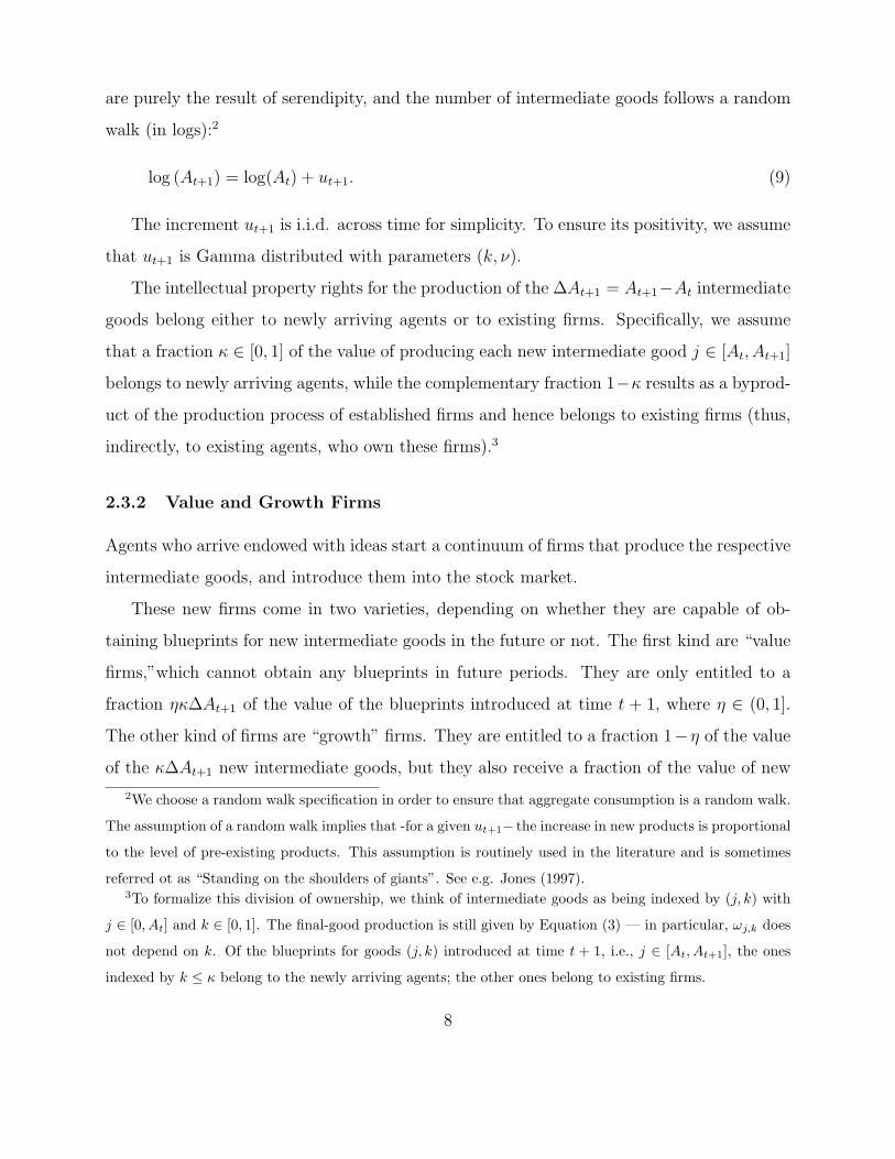
2.3.2 Value and Growth Firms
Agents who arrive endowed with ideas start a continuum of firms that produce the respective
intermediate goods, and introduce them into the stock market.
These new firms come in two varieties, depending on whether they are capable of ob-
taining blueprints for new intermediate goods in the future or not. The first kind are “value
firms,”which cannot obtain any blueprints in future periods. They are only entitled to a
fraction ηκΔAt+1 of the value of the blueprints introduced at time t + 1, where η ∈ (0, 1].
The other kind of firms are “growth” firms. They are entitled to a fraction 1−η of the value
of the κΔAt+1 new intermediate goods, but they also receive a fraction of the value of new
2We choose a random walk specification in order to ensure that aggregate consumption is a random walk.
The assumption of a random walk implies that -for a given ut+1− the increase in new products is proportional
to the level of pre-existing products. This assumption is routinely used in the literature and is sometimes
referred ot as “Standing on the shoulders of giants”. See e.g. Jones (1997).3To formalize this division of ownership, we think of intermediate goods as being indexed by (j, k) with
j ∈ [0, At] and k ∈ [0, 1]. The final-good production is still given by Equation (3) — in particular, ωj,k does
not depend on k. Of the blueprints for goods (j, k) introduced at time t + 1, i.e., j ∈ [At, At+1], the ones
indexed by k ≤ κ belong to the newly arriving agents; the other ones belong to existing firms.
8

Fractions of new blueprint value accruing to:
New value firms (owned by
)
New growth firms (owned by new agents)
Fractions obtained by growth firms of (1 )
new agents)gage 1,2,3…
1
11 t s
Old growth firms (owned by existing agents)
Firm age (t-s)g ( )
Figure 1: Illustration of the allocation of new blueprint value
blueprints in future periods. Specifically, in period n, growth firms born at s ∈ (−∞, n− 1]
obtain a fraction
(1 − κ)
(1 −�
�
)�n−s (10)
of the value of the ΔAn new blueprints. To simplify matters, we assume that there are no
intra-cohort differences between growth firms and any two growth firms of the same cohort
obtain the same value of blueprints in any given period. The geometric decay in the fraction
of new blueprints that accrues to a given growth firm as a function of its age ensures that
asymptotically the market capitalization of any growth firm goes to zero as a fraction of
aggregate market capitalization.
2.3.3 Workers
New business owners make up a fraction φ ∈ (0, 1) of newly arriving agents. The rest of the
newly arriving agents are workers. Workers arrive in life with an endowment of hours h . As
in Blanchard (1985), the endowment of hours changes geometrically with age at the rate δ,
so that a worker who was born at time s < t has an endowment of hours equal to ht,s =
9

h (1 − δ)t−s at time t. For simplicity, agents have no utility of leisure and supply their hours
inelastically.
In the real world younger workers are likely to be more productive in the presence of
increased technological complexity than older workers. One potential reason is that their
education gives them the appropriate skills for understanding the technological frontier. By
contrast, older workers are likely to be challenged by technological advancements. In Ap-
pendix B we present a simple vintage model of the labor market that introduces imperfect
substitution across labor supplied by agents born at different times. To expedite the presen-
tation of the main results, in this section we assume that labor is a homogenous good and
that workers’ endowment of efficiency units depreciates in a way that replicates the outcome
of the more elaborate model in Section 6.
Specifically, we assume that a worker’s total supply of efficiency units of labor is given
by ht,sqt,s with
log(qt+1,s) = log(qt,s) − ρut+1, (11)
and ρ ≥ 0. This specification captures the idea that advancements of the technological
frontier act as depreciation shocks to the productivity of old agents. In addition to being
intuitively appealing, this feature generates cohort effects in consumption that are consistent
with, and can be estimated directly from, the data. We undertake this exercise in Section 5.1.
To ensure a constant number of efficiency units in the economy, we normalize the initial
endowment of efficiency units to
qs,s = 1 − (1 − λ) (1 − δ) e−ρut+1 , (12)
and assume that (1 − λ) (1 − δ) ≤ 1. We also normalize the initial endowment of hours to
h = 1λ. This implies that the number of per-worker efficiency units, Lt/ (1 − φ), is always
equal to 1, and hence ht,sqt,s can be interpreted as the fraction of total wages that accrues
to workers born at time s.4
4Note that our assumptions imply
Lt
(1 − φ)= λ
∑s=−∞...t
[(1 − λ) (1 − δ)]t−sqt,s,
10

2.4 Asset Markets
Once born, agents face dynamically complete markets. This means that at each point in
time agents are able to trade in zero net supply Arrow-Debreu securities on the realization
of next period’s shocks εt+1 and ut+1. This assumption implies the existence of a stochastic
discount factor ξt, so that the time-s value of a claim paying a stream of dividends Dt with
limt→∞Es [ξtDt] = 0 is given by Es∑∞
t=s
(ξtξs
)Dt.
Finally, agents have access to annuity markets as in Blanchard (1985). (We refer the
reader to that paper for details). The joint assumptions of dynamically complete markets
for existing agents and frictionless annuity markets simplifies the analysis considerably, since
in a dynamically complete market with annuities an agent’s feasible consumption choices are
constrained by a single intertemporal budget constraint. For a worker, that intertemporal
budget constraint is given by
Es
∞∑t=s
(1 − λ)t−s(ξtξs
)cwt,s = Es
∞∑t=s
(1 − λ)t−s(ξtξs
)wtqt,sht,s, (13)
where cwt,s denotes the time-t consumption of a representative worker who was born at time s.
The left hand side of (13) represents the present value of a worker’s consumption, while the
right hand side represents the present value of her income. Similarly, letting cet,s denote the
time-t consumption of a representative inventor who was born at time s, her intertemporal
budget constraint is
Es
∞∑t=s
(1 − λ)t−s(ξtξs
)cet,s =
1
λφVs,s, (14)
where Vs,s is the time-s total market capitalization of new firms created at time s. The left-
hand side of equation (14) is the present value of a representative inventor’s consumption,
so that iterating forward once to obtain Lt+1(1−φ) and using (11) and (12) give
Lt+1
(1 − φ)= λ
∑s=−∞...t+1
(1 − λ) (1 − δ)t+1−sqt+1,s
= (1 − λ) (1 − δ)(
Lt
1 − φ
)e−ρut+1 + λhqt+1,t+1.
Setting qt+1,t+1 as in (12) implies Lt+1(1−φ) = Lt
(1−φ) = 1.
11

while the right-hand side is the value of all new firms divided by the mass of new business
owners (λφ) . To determine the total market value of firms (newly) created at time s, let Πj,s
be the fair value of the ability of firm j to produce a new intermediate good as given by the
net present value of the associated profits:
Πj,s =
[Es
∞∑t=s
(ξtξs
)πIj,t
]. (15)
The total market capitalization of all new firms can consequently be written as
Vs,s = κ
∫ As
As−1
Πj,sdj +
(1 −�
�
)Es
∞∑t=s+1
(ξtξs
)(1 − κ)�t−s
∫ At
At−1
Πj,tdj. (16)
The first term in equation (16) is the value of the blueprints for the production of new
intermediate goods that are introduced by new firms (both “growth” and “ value” firms) at
time s. Similarly the latter term captures the value of “growth opportunities,” i.e., the value
of blueprints to be received by growth firms in future periods.
2.5 Equilibrium
The definition of equilibrium is standard. To simplify notation, we let φe and φw denote the
fraction of entrepreneurs and workers (respectively) in the population so that
φi =
⎧⎨⎩ φ if i = e
1 − φ if i = w. (17)
An equilibrium is defined as follows
Definition 1 An equilibrium is defined as a tuple of adapted stochastic processes {xj,t, LFt ,cwt,s, c
et,s, ξt, pj,t, wt} where j ∈ [0, At] and t ≥ s such that
1. (Consumer optimality): Given ξt, the process cwt,s (respectively, cet,s) solves the opti-
mization problem (2) subject to the constraint (13) (respectively, constraint (14)).
2. (Profit maximization) The prices pj,t solve the optimization problem (8) and LFt , xj,t
solve the optimization problem (6) given pj,t, wt.
12

3. (Market clearing). Labor and goods markets clear
LFt + LIt = (1 − φ) (18)
λt∑
s=−∞
∑i∈{w,e}
(1 − λ)t−s φicit,s = Yt. (19)
Conditions 1 and 2 are the usual optimality conditions. Condition 3 requires that total
labor demand LFt + LIt equals total labor supply 1 − φ. Finally, the last condition requires
that aggregate consumption be equal to aggregate output.
3 Solution
3.1 Equilibrium Output, Profit, and Wages
We start with the intermediate goods and the labor markets. As a first step, we derive the
demand curve of the final goods firm for the intermediate input j at time t. Maximizing (6)
with respect to xj,t, we obtain
xj,t = LFt
[pj,t
ωj,tZtα
] 1α−1
. (20)
Substituting this expression into (8) and maximizing over pj,t leads to
pj,t =wtα, (21)
while combining (20) and (21) yields
xj,t = LFt
[wt
ωj,tZtα2
] 1α−1
. (22)
Turning to labor markets, maximizing (6) with respect to LFt gives the first order condi-
tion
wtLFt = (1 − α)Yt. (23)
13

Substituting (22) into (3) and then into (23) and simplifying yield
wt =(α2)α(1 − α
1 + χ
)1−αZtA
1−αt . (24)
Substituting equation (24) into (22) and then into (18) allows us to obtain the following
expressions for xj,t and LFt
xj,t =1 + χ
At
(j
At
)χ(1 − φ)α2
α2 + 1 − α(25)
LFt =1 − α
α2 + 1 − α(1 − φ) . (26)
Combining (25) and (26) inside (3) leads to the following simple expression for aggregate
output:
Yt =(α2)
α(
1−α1+χ
)1−α
α2 + 1 − α(1 − φ)ZtA
1−αt . (27)
An interesting feature of equation (27) is that the number of intermediate inputs (At) is
raised to the power 1 − α. This means that aggregate output is increasing as the number
of intermediate inputs increases. However, the extent of the increase depends on the degree
of subsitutability between different varieties of intermediate goods. For instance, as α ap-
proaches 1 existing and new intermediate goods become perfect substitutes, and so the only
effect of increases in variety is that newly arriving technologies “steal business” from existing
ones, without changing the overall productive capacity of the economy.
Before proceeding, it is useful to compute the income shares of labor and the profits of
the firms in the economy. Combining (24) and (27) implies that total payments to labor
wt (1 − φ) are simply equal to a fraction (α2 + 1 − α) of output Yt.Because of constant returns
to scale in the production of final goods the profits of the final goods firm are given by πFt = 0.
The profits to an intermediate goods producer are obtained by combining (25) and (21) with
(8) and (24) to obtain
πIj,t = (1 + χ)
(j
At
)χYtAtα (1 − α) . (28)
An interesting observation about (28) is that πIj,t is not cointegrated with Yt, since over time
At increases and hence asymptotically πIj,t/At → 0 almost surely. The lack of cointegration
14

between the dividends of an individual firm and aggregate output is to be expected because
of the constant arrival of competitors. Nevertheless, aggregate profits are a constant fraction
of total output, since∫ At0πIj,tdj = α (1 − α)Yt. This follows in a straightforward way, since in
a general-equilibrium framework the total income shares must add up to aggregate output:
wt (1 − φ) + πFt +∫ At
0πIj,tdj = Yt.
3.2 The Stochastic Discount Factor
To determine the stochastic discount factor ξt, we recall that, since agents face dynamically
complete markets after their birth, a consumer’s lifetime consumption profile can be obtained
by maximizing (2) subject to a single intertemporal budget constraint (constraint [13] if the
agent is a worker and constraint [14] if the agent is an inventor). Attaching a Lagrange mul-
tiplier to the intertemporal budget constraint, maximizing with respect to cit,s, and relating
the consumption at time t to the consumption at time s for a consumer whose birth date is
s gives
cit,s = cis,s
(C
(1−ψ)(1−γ)t
Cs(1−ψ)(1−γ)β−(t−s) ξt
ξs
)− 1γ
for i ∈ {e, w}. (29)
From this equation, the aggregate consumption at any point in time is
Ct = λ
t∑s=−∞
∑i∈{w,e}
(1 − λ)t−s φicis,s
(C
(1−ψ)(1−γ)t
Cs(1−ψ)(1−γ)β−(t−s) ξt
ξs
)− 1γ
, (30)
where φi was defined in (17). Iterating forward once to obtain Ct+1 and then using (30)
gives
Ct+1 = (1 − λ)Ct
(β−1 C
(1−ψ)(1−γ)t+1
Ct(1−ψ)(1−γ)ξt+1
ξt
)− 1γ
+ λ∑i∈{w,e}
φicit+1,t+1. (31)
Dividing both sides of (31) by Ct, solving forξt+1
ξtand noting that Ct = Yt in equilibrium
leads to
ξt+1
ξt= β
(Yt+1
Yt
)−1+ψ(1−γ)⎡⎣ 1
1 − λ
⎛⎝1 − λ∑i∈{w,e}
φicit+1,t+1
Yt+1
⎞⎠⎤⎦−γ
. (32)
15

To obtain an intuitive understanding of equation (32) it is easiest to focus on the case ψ = 1,
so that agents have standard CRRA preferences. In this case, the stochastic discount factor
consists of two parts. The first part is β(Yt+1
Yt
)−γ, which is the standard expression for the
stochastic discount factor in an (infinitely-lived) representative-agent economy. The second
part — the term contained inside square brackets in equation (32) — gives the proportion
of output at time t+1 that accrues to agents already alive at time t. To see this, note that
only a proportion 1 − λ of existing agents survive between t and t + 1, and that the newly
arriving generation claims a proportion 1 − λ∑
i∈{w,e} φi cit+1,t+1
Yt+1of aggregate output. The
combination of the two parts yields the consumption growth between t and t + 1 of the
surviving agents.
Equation (32) states an intuitive point: Since only agents alive at time t are relevant
for asset pricing, it is exclusively their consumption growth that determines the stochastic
discount factor, not the aggregate consumption growth. We elaborate on this point further
in the next section.
To conclude the computation of equilibrium, we need to obtain an expression for the
term inside square brackets on the right-hand side of (32). This can be done by using the
intertemporal budget constraints (14) and (13). Proposition 1 in the Appendix shows that
1 − λ∑i∈{w,e}
φicit+1,t+1
Yt+1
= υ(ut+1; θe, θw, θb),
with
υ(ut+1; θe, θw, θb) ≡ 1 − θeα (1 − α)
(κ(1 − e−(1+χ)ut+1
)+
(1 −�
�
)θb)
(33)
−θw (α2 + 1 − α) (
1 − (1 − λ) (1 − δ) e−ρut+1),
and θe, θb, θw are three appropriate constants obtained from the solution of a system of three
nonlinear equations in three unknowns. Given the interpretation of υ(ut+1; θe, θw, θb) as the
fraction of consumption that accrues to new agents, we shall refer to it as the “displacement
factor”.
16

4 Qualitative Properties
As we already discussed, equation (32) captures the intuition that only the consumption of
existing agents matters for the stochastic discount factor. A first implication of this fact is
that the commonly used consumption CAPM (using aggregate consumption data) may fail
in explaining asset returns. The easiest way to illustrate this point is to consider a limiting
case of our model in which the consumption CAPM (using aggregate data) would yield that
all risk premia are zero.
Specifically, suppose that σ = 0, ρ > 0 and α approaches 1. Equation (27) implies that
the volatility of output approaches zero. In a standard model, therefore, equity premia would
approach zero, as well. However, this is not the case in our model, as the following Lemma
illustrates.
Lemma 1 Assume that σ = 0, ρ > 0, κ = 1, and
1 > β (1 − λ)γ eμψ(1−γ) (34)
1 ≤ β (1 − δ)−γ E[eργut+1 ]. (35)
Then, letting Rt be the return of any stock, an equilibrium exists and
limα→1
V ar (ΔYt+1) = 0 (36)
limα→1
∂(ξt+1/ξt
)∂ut+1
> 0 (37)
limα→1
{E(Rt) −
(1 + rf
)}> 0. (38)
Conditions (34)–(35) are technical conditions, both necessary and sufficient for the exis-
tence of an equilibrium. They are satisfied for a wide range of parameter combinations and
distribution functions.
The intuition behind Lemma 1 is straightforward. Even though the volatility of aggre-
gate consumption becomes negligible as α approaches 1, the volatility of existing agents’
consumption doesn’t. As α approaches 1, the competition between firms is fierce, as all
intermediate inputs start becoming perfect substitutes. This implies that new innovations
17

result almost exclusively in redistribution from old to young firms and from old to young
agents (since ρ > 0). Since it is only the consumption growth of existing agents that matters
for asset prices, innovation shocks (ut) present “aggregate” shocks for existing agents, even
though they are not “aggregate” shocks from the perspective of the entire economy. Since
the profits of existing firms are exposed to these innovation shocks (ut), existing companies’
stock exposes agents to these shocks and commands a risk premium.
Even though the limiting case α = 1 is clearly an extreme special case of the model,5
the results in Lemma 1 help explain why asset pricing based on the standard (aggregate)
consumption CAPM relationship can understate the risks associated with investing in stocks
from the perspective of existing agents.
The distinction between consumption of current agents and aggregate consumption has
also important implications for the value premium. To start, assume henceforth that κ < 1,
so that “growth firms” receive a fraction of the value of new blueprints over time. Letting Πs
be given as in (15), define the price to earnings ratio q for a typical value firm as q ≡ Πsπs. Since
the increments to the (log) stochastic discount factor and the increments to (log) profits of
value firms are i.i.d., q is a constant.6 Then, for any set of parameter values such that there
exists a solution to (52)–(54) we have the following Lemma.
Lemma 2 The (end of) period-t value of the representative “growth firm” created at time s
is given by
Pt,s = α (1 − α)Yt
[(q − 1)Nt,s + (1 −�)�t−s θ
b
�q
], (39)
5A caveat behind Lemma 1 is that in the limit α = 1 the profits of intermediate goods firms disappear.
Hence, even though the rate of return on a stock is well defined in the limit (because rates of returns are
not affected by the level of dividends and prices), the limiting case α = 1 is of limited practical relevance.
However, it has theoretical interest, because it illustrates in a simple way the asset pricing implications of
the wedge between aggregate consumption and existing agents’ consumption.6We show this formally as part of the proof of Proposition 1.
18

where
Nt,s = (1 − η)κ
(AsAt
)1+χ (1 − e−(1+χ)us
)+
t∑n=s+1
(1 −�) (1 − κ)�n−(s+1)
(AnAt
)1+χ (1 − e−(1+χ)un
).
The first term inside the square brackets in equation (39) is the value of all the blueprints
that the growth firm has received since its creation, while the second term is the value of
remaining growth opportunities. Based on (39), the (gross) rate of return of the representa-
tive “growth firm” Rgt+1 at time t+ 1 is given by the dividends from pre-existing blueprints
α (1 − α)Yt+1Nt, the dividends from the new blueprints α (1 − α)Yt+1 (Nt+1 −Nt), and the
end of period price Pt+1,s, all divided by the beginning of the period price Pt,s :
Rgt+1,s ≡
α (1 − α)Yt+1Nt+1 + Pt+1,s
Pt,s.
It will be useful to decompose this expression into two components. Specifically, define the
gross rate of return of a “pure” value firm RIt+1 and the gross rate of return of a “pure”
growth firm Rot+1 as7
RIt+1 =
(q
q − 1
)(πt+1
πt
), (40)
Rot+1 = �
(Yt+1
Yt
)(1 − κ)
(1 − e−(1+χ)ut+1
)+ θb
θb. (41)
Then, the rate of return on any growth firm can be expressed as
Rgt+1,s =
(1 − wot,s
)RIt+1 + wot,sR
ot+1, (42)
where wot,s is the relative weight of growth options in the value of the firm, and is obtained
from Lemma 2 as
wot,s =(1 −�)�t−s θb
q
(q − 1)Nt + (1 −�)�t−s θb q.
7A pure value firm is one that receives no new blueprints. A pure growth firm is one that has no blueprints
currently, but will receive a geometrically decaying number of such blueprints in each future year.
19

Expressions (40) and (41) imply that RIt+1 and Ro
t+1 are exposed differently to innovation
shocks ut. Specifically, equations (28) and (27) imply that∂RIt+1
∂ut+1< 0, while
∂Rot+1
∂ut+1> 0. Hence,
if the marginal utility of existing agents increases in response to ut shocks (mathematically,∂(ξt+1/ξt)∂ut+1
> 0), these agents will require a higher rate of return to hold value stocks than
growth stocks. The reason is that the growth opportunities embedded in growth stocks act
as a hedge against ut shocks and hence drive the return of growth stocks down. Equation
(37) of Lemma 1 asserts that this will be the case whenever α is close enough to 1.8
We conclude this section with a few remarks on the relationship between the equilibrium
stochastic discount factor in our model and some popular asset pricing models, such as the
CAPM and the consumption-CAPM.
A closer inspection of equations (33), (32) and (27) reveals that both the increments of
the (log) stochastic discount factor and the increments to (log) aggregate consumption are
i.i.d.. Hence, equation (29) implies that a consumer’s (log) lifetime consumption process is
a random walk with drift, and the ratio of an agent’s wealth to her current consumption(W i
t,s/cit,s
)is constant for all t and s9. Therefore equation (29) can be re-written as
W it,s = W i
s,s
(C
(1−ψ)(1−γ)t
Cs(1−ψ)(1−γ)β−(t−s) ξt
ξs
)− 1γ
for i ∈ {e, w}. (43)
Letting W t denote aggregate wealth in the economy, and repeating the same steps as in
equations (30)-(32) implies
ξt+1
ξt= β
C(1−ψ)(γ−1)t+1
Ct(1−ψ)(γ−1)
⎧⎨⎩ 1
1 − λ
W t+1
[1 − λ
(φw
Wwt+1,t+1
W t+1+ φe
W et+1,t+1
W t+1
)]W t
⎫⎬⎭−γ
. (44)
8We note that equation (37) continues to hold when σ > 0, after a few minor modifications of the technical
conditions of the Lemma.9To see this, note that at any point in an agent’s life her consumption and her total wealth W i
t,s (the sum
of financial wealth and human capital) are related through the net present value relationship
W it,s = ct,sEt
∞∑u=t
(1 − λ)u−t
(cu,s
ct,s
)(ξu
ξt
).
Because both cu,s
ct,sand ξu
ξtare random walks (with drift) in logarithms, the expectation on the right hand
side of the above equation is a constant and the result follows.
20

Equations (32) and (44) are equivalent ways of expressing the stochastic discount factor.
However, they produce different insights as to why some standard asset pricing models fail
within our model. As we have already discussed, equation (32) implies that the consumption
CAPM (implemented empirically by using aggregate consumption data) will not hold.
Equation (44) shows why the conventional CAPM also does not hold in our model. At
first pass, equation (44) implies that if ψ = 1, then variations in the stochastic discount
factor are identifiable with changes in the total wealth of pre-existing agents. (To see this,
note that the term inside square brackets in equation (44) simply subtracts the wealth that
accrues to newly arriving agents from the total wealth in the economy at time t + 1). One
might therefore conjecture that since all stocks are held by pre-existing agents, and newly
arriving agents have no financial wealth, it might be possible to use the CAPM to identify
changes in the wealth of pre-existing agents. The problem with this argument is that the
total wealth of pre-existing agents is comprised of both human and financial wealth. As long
as the two are not perfectly correlated (or if ψ = 1), the CAPM will not hold.
Since the usual approaches to quantifying the variability of the stochastic discount fac-
tor are inadequate, in the next section we employ an alternative approach to quantify the
variation of the stochastic discount factor. This approach estimates directly changes in the
consumption of pre-existing agents by using microeconomic data and cohort analysis.
5 Quantitative Evaluation
5.1 Cohort Effects and Asset Returns
The model has robust novel implications for the joint behavior of consumption cohort effects
and cross-sectional asset-pricing returns. In this section we derive these implications and
test them in the data. In the next section we use the moments that we estimate here to
calibrate the model.
Taking logarithms on both sides of (29), we obtain the following decomposition of an
agent’s consumption into a cohort effect (as) , a time effect (bt) and an individual specific
21

effect εi for i ∈ {e, w}:
log cit,s = as + bt + εi, (45)
where
as =∑
j∈{e,w}φj log cjs,s +
1
γlog
(C(1−ψ)(1−γ)s β−sξs
), (46)
bt = −1
γξtβ
−tC(1−ψ)(1−γ)t , (47)
εi = log cis,s −∑
j∈{e,w}φj log cjs,s (48)
Equation (45) provides a first testable implication of the model: In a model with unrestricted
transfers between altruistically linked generations, every agent’s consumption is a constant
proportion of the aggregate consumption regardless of her birth date.10 Consequently, cohort
effects are zero in such a model. By contrast, in our model log consumption exhibits non-
zero cohort effects. The following lemma derives the dynamic behavior of these cohort effects
according to the model.
Lemma 3 Let zs be defined as
zs ≡ (1 − φ) log
(cws,sYs
)+ φ log
{ces,sYs
}Then for any T ≥ 1,
as+T − as = −T∑i=1
log
(υ (us+i)
1 − λ
)+ zs+T − zs. (49)
Equation (49) implies that cohort effects should be non-stationary according to our model,
since the first term on the right hand side of (49) is a random walk with drift. Moreover, as
we show in the Appendix11, zs is i.i.d. and captures the fraction of income accruing to newly
arriving agents at time s. Another interesting implication of (49) is that the increments
10Such a model is isomorphic to the standard infinitely-lived representative-agent model.11We show this as part of the proof of Proposition 1.
22
to the random walk component of the consumption cohort effects “reveal” the unobserved
displacement factor υ (us) . Specifically, taking (de-meaned) first differences of the cohort
effects Δas+i and forming an estimate of their “long run” variance by a heteroscedasticity-
and autocorrelation-consistent variance estimator (such as Newey-West) gives a consistent
estimate of the variance of log(�υ(us+i)
1−λ
). This provides useful guidance in calibrating the
model, since we can obtain a measurement of the variance of the displacement factor.
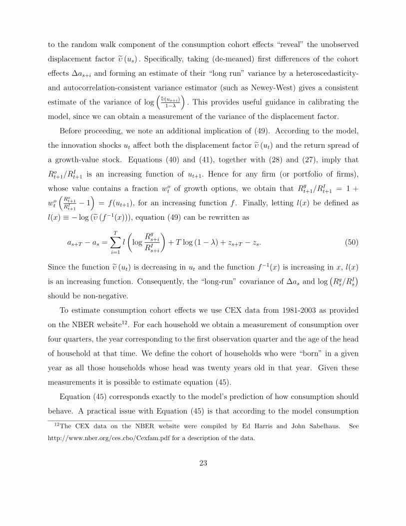
Before proceeding, we note an additional implication of (49). According to the model,
the innovation shocks ut affect both the displacement factor υ (ut) and the return spread of
a growth-value stock. Equations (40) and (41), together with (28) and (27), imply that
Rot+1/R
It+1 is an increasing function of ut+1. Hence for any firm (or portfolio of firms),
whose value contains a fraction wot of growth options, we obtain that Rgt+1/R
It+1 = 1 +
wot
(Rot+1
RIt+1− 1
)= f(ut+1), for an increasing function f . Finally, letting l(x) be defined as
l(x) ≡ − log (υ (f−1(x))), equation (49) can be rewritten as
as+T − as =T∑i=1
l
(log
Rgs+i
RIs+i
)+ T log (1 − λ) + zs+T − zs. (50)
Since the function υ (ut) is decreasing in ut and the function f−1(x) is increasing in x, l(x)
is an increasing function. Consequently, the “long-run” covariance of Δas and log(Rgs/R
Is
)should be non-negative.
To estimate consumption cohort effects we use CEX data from 1981-2003 as provided
on the NBER website12. For each household we obtain a measurement of consumption over
four quarters, the year corresponding to the first observation quarter and the age of the head
of household at that time. We define the cohort of households who were “born” in a given
year as all those households whose head was twenty years old in that year. Given these
measurements it is possible to estimate equation (45).
Equation (45) corresponds exactly to the model’s prediction of how consumption should
behave. A practical issue with Equation (45) is that according to the model consumption
12The CEX data on the NBER website were compiled by Ed Harris and John Sabelhaus. See
http://www.nber.org/ces cbo/Cexfam.pdf for a description of the data.
23

only features time and cohort effects, but no age effects. Realistically, one would expect
the presence of age effects either because of borrowing constraints early in life, or because
of changes in the consumption patterns of households as children age, etc. In order to be
conservative with the attribution of consumption variation to cohort effects, we estimated
(45) allowing for age effects. We also include a control for (log) household size.13
An issue that arises when we include age effects in (45) is that linear trends in age, cohort,
and time effects cannot be identified separately.14 Fortunately, the exact identification of
the linear trends is immaterial for our purposes. As has been shown in the literature, it
is possible to estimate differences in differences of cohort effects (as+1 − as − (as − as−1))
without any normalizing assumption and even after including a full set of age dummies.15 16
An implication of this statement is that there exists a function of time a∗s such that, for any
normalizing assumptions, the estimated cohort effects as are given by as = β0+β1s+a∗s. (The
coefficients β0 and β1 are not identified, i.e., their magnitude depends on the normalizing
assumptions.)
According to our model, a∗s is non-zero, but instead behaves like a random walk. Hence
the first hypothesis we test is that a∗s = 0. The three columns of Table 1 report the results
of estimating equation (45) including 1) no age effects, 2) parametric age effects, and 3) a
full set of age dummies. The model with parametric age effects is fitted by assuming that
age effects are given by some function h (age) which we parameterize with a cubic spline
13We also adjusted for family size by dividing by the average family equivalence scales reported in
Fernandez-Villaverde and Krueger (2007) and the results remained unchanged.14Sometimes the literature addresses this problem by following Deaton and Paxson (1994) and making
the normalizing assumption that the time effects add up to zero and are orthogonal to a time trend. In our
model the time effects bt follow a random walk and hence such an assumption is not appropriate.15See McKenzie (2006) for a proof.16The easiest way to see this, is to allow for age effects in equation (45), consider the resulting equation
log cit,s = as + bt + γt−s + εi, and observe that
E log cit+1,s+1 − E log ci
t+1,s −(E log ci
t,s − E log cit,s−1
)= as+1 − as − (as − as−1) .
Replacing expectations with the respective cross sectional averages shows how the differences in differences
of cohort effects (as+1 − as − (as − as−1)) can be estimated in the data.
24

No age effects Parametric Age Effects Age Dummies
Wald Test a∗ = 0 31.3 4.21 4.25
p-value 0.000 0.000 0.000
Observations 52245 52245 52245
R-squared 0.373 0.382 0.384
Table 1: Results from regression of log consumption expenditure on quarter dummies, a control
for log(fam.size) and various specifications of cohort and age effects. Cohort effects are included
via cohort dummies. In the first specification the regression does not contain age effects, while
the second specification allows age effects parameterized via a cubic spline. The third specification
allows for a full set of age dummies. The Wald test refers to the test that as+1−as−(as−as−1) = 0
for all s. Standard errors are computed using a robust covariance matrix clustered by cohort and
quarter. The CEX data are from 1980-2003 and include observations on cohorts as far back as
1911.
having knots at ages 33, 45, and 61. The first row reports the results from a Wald test that
the estimated differences as+1 − as − (as − as−1) = 0 for all s. The second row reports the
associated p−values. As can be seen, the data strongly reject the hypothesis that cohort
effects are either non-existent or given by a deterministic linear trend. For our purposes, this
implies that we can reject the prediction of a standard representative-agent model, namely
that cohort effects are uniformly zero.
The first two rows of Table 2 report results on the magnitude of the variation of these
cohort effects for different ways of accounting for age effects. The first row contains informa-
tion on the standard deviation of the first differences of cohort effects (as+1− as). The second
row fits an ARIMA (1,1,1) to as and then uses the methods of Beveridge and Nelson (1981)
to obtain the standard deviation of the permanent component of as. As two alternative ways
to obtain an estimate of this standard deviation, we report in the third row Newey-West
estimates of the long-run variance of the first differences of as using 10-year autocovariance
lags. In the fourth row we report the standard deviation of cohort effects summed over
25

Param. Age Effects Age Dummies
Std. Dev. (Cohort−Lagged Cohort) 0.030 0.030
Std. Dev. (Perm. Component (Newey West)) 0.020 0.020
Std. Dev. (Perm. Component (Beveridge Nelson)) 0.021 0.023
Std. Dev. (Perm. Component√
10(10-year Aveg)) 0.019 0.018
Cov(coh.diffs; FF)Var( coh.diffs)
(Newey West) 3.39 3.92
Cov(10-year coh.diffs; 10-year FF)Var(10-year coh.diffs)
2.93 3.43
Observations 68 68
Table 2: Various moments of the permanent components of the estimated cohort effects.
10-year intervals, computing the associated standard deviation, and dividing by√
10. All
methods yield roughly similar results. We use these estimates in the next section, when we
calibrate the model.
To obtain a visual impression of these results, the solid line in Figure 2 depicts the esti-
mated cohort effects.17 As can be seen from the figure, these cohort effects are persistent,
in line with the results reported in the first two rows of Table 2. The dashed line depicts∑Ti=1 log
(Rgt+i/R
It+i
), where we have used the negative of the logarithmic gross return as-
sociated with the HML factor of Fama and French (1992) as a measure of log(Rgt+i/R
It+i
)and have removed a linear trend. According to Equation (50), the consumption cohort ef-
fects should be co-trending with the sum of an appropriate non-linear increasing function
l(log(Rgt+1/R
It+1
)). Assuming that l(·) is reasonably well approximated by an affine first or-
der Taylor expansion, cohort effects and cumulative (log) returns on a growth-value portfolio
should be co-trending, as the picture suggests.
For the purpose of the calibration exercise that follows, a useful quantity is the covari-
ance between the innovations to the permanent components of as and to the permanent
17We report the cohort effects from 1927 onward, since data on the Fama French factors are available
from 1927 onward. We also report results up to 1995 because of the sparsity of data on cohorts post 1995.
However, cohort effects prior to 1927 and post 1995 are included in the estimation and all testing exercises.
26

cum FF factor (detrended)
consumption cohorts (detrended)
−.1
5−
.1−
.05
0.0
5.1
1920 1940 1960 1980 2000cohort
Figure 2: Consumption cohort effects and cumulative returns on a growth-value portfolio
(negative of the HML factor) after removing a constant time trend from both series and
multiplying the latter series by a scalar to fit in one scale. A full set of age dummies was
used in estimating the consumption cohort effects.
components of∑s
i=1 log(Rgt+i/R
It+i
). According to (50), the covariance between the inno-
vations to these permanent components (to which we will refer as the long-run covariance)
provides a measure of cov(log(Rgt /R
It
), log υ (ut)), i.e. a measure of how the displacement
factor covaries with the returns to a growth-value portfolio. We obtain an estimate of this
covariance by using a multivariate Newey-West (10 lags) estimate of the covariance between
the negative of the logarithmic gross return associated with the HML factor and the first
differences of the estimated cohort effects. The fifth row of Table 2 reports this covariance,
normalized by the long-run variance of the consumption cohort effects as obtained in the
second row of the table. As a robustness check, we also report in the final row of the table
27

the results from computing the covariance of 10-year consumption cohort differences and 10-
year cumulative returns on the growth-value portfolio, normalized by the variance of 10-year
consumption-cohort differences.
Table 3 reports results on a stronger implication of the model, namely that the permanent
component of cohort effects can help explain return differentials of stocks in different book
to market deciles. Specifically, the second line of this table reports the average return
differential between the (log) gross return of a portfolio of stocks with book to market values
in various deciles vs. the respective return of a portfolio in the 10th decile. The third row
of table 3 reports the analog of the 5th row of table 2 for these return differentials, namely
the covariance between these return differentials and the first differences of the permanent
component of (log) consumption cohort effects (normalized by the variance of the permanent
component of these cohort effects). Consistent with the empirically well established value
premium, stocks with lower book to market values (growth stocks) exhibit a lower return
than stocks with higher book to market values (value stocks). Interpreting the (permanent
component of) consumption cohort effects as a measure of the displacement factor, the model
implies that stocks in lower deciles should act as hedges compared to the stocks in the top
decile. That is, the covariance between the (permanent component of) consumption cohort
effects and the ith − 10 return differential should be negative, and higher in absolute value,
the smaller is i. This is the general pattern in the last row of the table.
Before proceeding with the calibration, we note that so far we have focused on the
empirical implications of the model for consumption and returns. This is of first-order
importance for asset pricing because these two quantities determine expected returns, which
are the focus of this paper. However, the model makes additional predictions, which allow us
to inspect further whether the model’s mechanisms can be detected in the data. An obvious
candidate, which also plays a role in the calibration of the model, is whether agents’ income
is affected by intergenerational risk. Applying a similar argument to the one that led to
Equation (45), Equations (11) and (12) imply the presence of cohort effects in income data
that should be correlated with the cumulative return of a growth-value portfolio. Figure 3 is
28
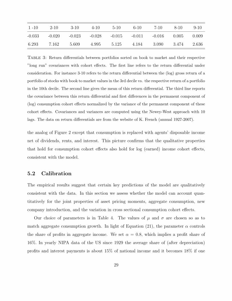
1 -10 2-10 3-10 4-10 5-10 6-10 7-10 8-10 9-10
-0.033 -0.020 -0.023 -0.028 -0.015 -0.011 -0.016 0.005 0.009
6.293 7.162 5.609 4.995 5.125 4.184 3.090 3.474 2.636
Table 3: Return differentials between portfolios sorted on book to market and their respective
”long run” covariances with cohort effects. The first line refers to the return differential under
consideration. For instance 3-10 refers to the return differential between the (log) gross return of a
portfolio of stocks with book to market values in the 3rd decile vs. the respective return of a portfolio
in the 10th decile. The second line gives the mean of this return differential. The third line reports
the covariance between this return differential and first differences in the permanent component of
(log) consumption cohort effects normalized by the variance of the permanent component of these
cohort effects. Covariances and variances are computed using the Newey-West approach with 10
lags. The data on return differentials are from the website of K. French (annual 1927-2007).
the analog of Figure 2 except that consumption is replaced with agents’ disposable income
net of dividends, rents, and interest. This picture confirms that the qualitative properties
that hold for consumption cohort effects also hold for log (earned) income cohort effects,
consistent with the model.
5.2 Calibration
The empirical results suggest that certain key predictions of the model are qualitatively
consistent with the data. In this section we assess whether the model can account quan-
titatively for the joint properties of asset pricing moments, aggregate consumption, new
company introduction, and the variation in cross sectional consumption cohort effects.
Our choice of parameters is in Table 4. The values of μ and σ are chosen so as to
match aggregate consumption growth. In light of Equation (21), the parameter α controls
the share of profits in aggregate income. We set α = 0.8, which implies a profit share of
16%. In yearly NIPA data of the US since 1929 the average share of (after depreciation)
profits and interest payments is about 15% of national income and it becomes 18% if one
29

Income cohorts (detrended)
cum FF. Factor (detrended)
−.1
−.0
50
.05
.1
1950 1960 1970 1980 1990 2000cohort
Figure 3: Earned (log) income cohort effects and cumulative returns on a growth-value
portfolio (negative of the HML factor) after removing a constant time trend from both series
and and multiplying the latter series by a scalar to fit in one scale.. A full set of age dummies
was used in estimating the income cohort effects. The regression was estimated with post-war
cohorts (1947 onward) to avoid discontinuities in earned income that arise at 65.
imputes that 1/3 of proprietor’s income is due to profits.18 The parameter λ is chosen so as
to capture the arrival of new agents. In post war data the average birth rate is about 0.016.
Immigration rates are estimated to be between 0.002−0.004, which implies an overall arrival
18Since in our model there is no financial leverage, it seems appropriate to treat both dividend and interest
payments as one entity. Moreover, it also seems appropriate to deduct depreciation from profits, because
otherwise the relative wealths of agents e and w would be unduly affected by a quantity that shouldn’t be
counted as income of either. The real business cycle literature assumes a profit share of 1/3 but also models
investment and depreciation explicitly and deducts investment from (gross) profits to obtain dividends. As
a result the share of (net) output that accrues to capital holders is close to the number we assume here.
30

rate of new agents between 0.018 and 0.02. We take the discount factor to be close to 1,
since in an OLG model the presence of death makes the “effective” discount factor of agents
equal to β(1 − λ). Given a choice of λ = 0.02, the effective discount rate is 0.98, consistent
with a standard choice in the literature.The constant ψ influences the growth of agents’
marginal utilities, and hence is important for the determination of interest rates. We choose
ψ = 0.5, in order to approximately match observed interest rates. On behavioral grounds,
this assumption implies that an individual places equal weights on his own consumption and
on his consumption relative to the aggregate.
In the model, the parameter δ controls age effects in income. In the real world, income
is hump shaped as a function of age. However, for the purpose of calibrating the model, it is
only the net present value of income at birth that affects the general-equilibrium outcomes.
With this in mind, we use the estimated age-(log) earnings profiles of Hubbard et al. (1994)
and determine δ so that
Es
∞∑t=s
(1 − λ)t−s(ξtξs
)(wtws
)(1 − δ)t−s
(AtAs
)−ρ
= Es
∞∑t=s
Λt−sG(t− s)
(ξtξs
)(wtws
)(AtAs
)−ρ,
where Λt−s is an agents’ survival probability at age t− s obtained from the National Center
for Health Statistics and G(t− s) is the age-(log) earnings profile, as estimated by Hubbard
et al. (1994).
To ensure positivity of ut we choose a Gamma distribution with parameters k, ν. The
parameters ρ and χ control the exposure of labor and dividend income to the shock ut. We
choose k, ν, ρ and χ so as to match a) the variation of permanent components of consumption
cohort effects as reported in Table 2, b) the variation of the permanent components of
income cohort effects, which we obtain by using earned log income (instead of consumption
expenditure) on the left hand side of Equation (45), estimating the resulting cohort effects
and isolating their permanent component, c) the volatility of aggregate dividends, and d)
the correlation between aggregate dividends and aggregate consumption.
The parameter κ gives the proportion of growth options that are tradeable, while �
31

β 0.999 k 0.25
ψ 0.5 ν 0.05
μ 0.015 ρ 0.9
σ 0.032 κ 0.9
α 0.8 χ 4
λ 0.018 ω 0.87
δ -0.012 η 0.9
Table 4: Baseline parameters used in the calibration.
controls the timing of the exercising of these options (higher � means that the options are
exercised sooner). As a consequence, these two parameters jointly determine the aggregate
price-to-earnings ratio, as well as the properties of growth firms. We therefore calibrate
them to the aggregate price-to-earnings ratio and the covariance between HML returns and
changes in the permanent component of consumption cohort effects.19
The parameter η does not affect aggregate valuation ratios, or the returns of a pure-
growth firm, but it controls the proportions of value and growth firms, and thus the properties
of the cross-section of valuation ratios. We calibrate it to the price-to-earnings ratio of the
top X% of the distribution. [What should X be? Why 90 and not 50? etc]
Finally, we treat the parameter γ as a free parameter and examine the model’s ability to
match a wide variety of moments for values of γ that generate reasonable equity and value
premia. Since we are attempting to match more moments than parameters, it is impossible
to obtain an exact fit, but the deviations between the data and the simulated moments
appear reasonably small. As can be seen in Table 5, with γ = 10 the model can match
about 66% of the equity premium and about 80% of the value premium. As γ increases to
12 the model does well in almost all dimensions. In interpreting these results, it should be
noted that the model has no role for financial or operating leverage, which, as Barro (2006)
19We chose this covariance over other moments because of its importance in the determination of the value
premium, which is central to the paper.
32

Data γ = 10 γ = 12 γ = 15
Aggregate (log) Consumption Growth rate 0.017 0.017 0.017 0.017
Aggregate (log) Consumption Volatility 0.033 0.032 0.032 0.032
Riskless Rate 0.010 0.022 0.015 0.014
Equity premium 0.061 0.040 0.051 0.062
Aggregate Earnings / Price 0.075 0.103 0.108 0.119
Dividend Volatility 0.112 0.10 0.101 0.101
Correl. (divid. growth, cons.growth) 0.2 0.189 0.189 0.189
Std (Δαperms ) 0.023 0.024 0.024 0.023
cov(Δαperms ,logRg−logRI)var(Δαperm
s ) 3.92 4.226 4.378 4.598
Std (Δwperms ) 0.022 0.023 0.023 0.023
Earnings / Price 90th Perc. 0.120 0.11 0.118 0.132
Earnings / Price 10th Perc. 0.04 0.041 0.039 0.041
Average Value premium 0.081 0.064 0.081 0.097
Std (Value Premium) 0.120 0.104 0.105 0.105
Expected Return Value - ”Pure” Growth 0.102 0.121 0.141
Table 5: Data and model calibration for different values of risk aversion γ. Data on con-
sumption, the riskless rate, the equity premium and dividends per share are from Campbell
and Cochrane (1999). Data on the aggregate E/P ratio are from the long sample (1871-2005)
on R. Shiller’s Website. The E/P for value and growth firms are the respective E/P ratios
of firms in the bottom 10% vs. top 90% of the cross sectional book to market distribution
from Fama and French (1992). The value premium is computed as the difference in value
weighted returns of stocks in the top 90%-bottom 10% of the cross sectional book to market
distribution, as reported in the website of Kenneth French. The two numbers in square
brackets for Std (Δαperms ) refer to the standard deviation of the permanent components of
consumption cohort effects as estimated in Table 2. Std (Δwperms ) refers to the respective
numbers for the cohort effects of earned income.
33

argues, implies that the unlevered equity premium produced by the model compared to the
levered equity premium produced by the data should be in a 2/3 ratio. Moreover, in the
model there is no time variation in interest rates, volatility, and excess returns. Therefore,
in light of the literature, it is not surprising that the model needs relatively high levels of
risk aversion in order to explain the data. However, it should be noted that even in the
absence of these effects, levels of risk aversion around 10 explain a non-trivial fraction of
asset-pricing data. Therefore, the evidence in Table 5 suggests that the model’s mechanisms
are quantitatively powerful enough to explain a substantial fraction of the equity premium,
the value premium, and the riskless rate.
5.3 Inspecting the mechanism
As the calibration shows, the model is successful in matching unconditional return moments.
A number of factors are responsible for this success, and here we take a closer look at the
quantitative significance of each factor.
The model produces large equity and value premia for three reasons: First, current agents’
consumption growth is more volatile than aggregate consumption growth, because of the
displacement effect. Second, current firms’ dividends are more sensitive to the displacement
factor than current agents’ consumption. And third, there is co-skewness between current
firms’ dividend growth and current agents’ consumption growth.
A simple back of the envelope calculation helps illustrate the magnitude of each factor.
Taking logarithms of the pricing kernel in equation (32 ), using (5), (27), and the definition
of υ(ut+1) in equation (33) leads to
Δ log ξt+1 − log β(1 − λ)γ − (−1 + ψ (1 − γ))μ
= (−1 + ψ (1 − γ))εt+1 − γυ(ut+1) + (−1 + ψ (1 − γ)) (1 − α)ut+1. (51)
At the same time, the stochastic component of the aggregate dividend growth equals εt+1 +
h(ut+1) for some function h.20 Given our choice of parameters ψ = 0.5, γ = 10 and σ = 0.032,
20According to equation (28), h(x) = −(1 + chi)x the existing value firms. However, since the dividends
34

the standard deviations of the first term in (51) is 0.18; the standard deviation of υ(ut+1)
is 0.023, so that of the second term is 0.23; and the last term has a standard deviation of
0.0275, which is an order of magnitude smaller and we therefore ignore for the purpose of
our illustration. As for the dividends, since their standard deviation of growth is about 0.1
and that of ε is 0.032, h(ut+1) has standard deviation of√
0.12 − 0.0322 = 0.095. Given that
the price-to-dividend ratio is constant, this is also the standard deviation of market (log)
returns.
Based on these standard deviations, if εt+1 and ut+1 (and therefore υ(ut+1), approxi-
mately) were both normal, then the equity premium would equal 0.18×0.032+0.23×0.095 =
0.028. The difference between this number and the 0.04 equity premium in our base-case cal-
ibration owes to the fact that ut+1 is a non-normal shock, making the consumption growth
of existing agents and the returns in the stock market co-skewed.
This back-of-the-envelope calculation shows that the bulk of the equity premium in our
model is not due to the fact that consumption of existing agents is excessively volatile. The
total volatility of existing agents’ consumption is approximately equal to 0.039, which is not
far away from the aggregate volatility of 0.032.
We conclude by noting that the model not only produces a sizeable equity premium, but
also an interest rate that is constant and low. The reasons are that a) current agents’s con-
sumption has a slightly lower mean growth rate (1.5%) than that of aggregate consumption
(1.7%) and is more volatile (3.9%) than aggregate consumption (3.2%), and b) external habit
formation (captured by ψ) implies that agents’ marginal utility of consumption declines more
slowly than suggested solely by risk aversion and consumption growth.
of existing growth firms also include the dividends from the blueprints that are created within the period, h
is generally different.
35

6 Extensions and Discussion
6.1 Frictions and blueprint endowments later in life
In order to be able to solve and analyze the model, we made several simplifying assumptions.
Here we verify the robustness of our findings to some of these assumptions. Specifically, one
of model’s stylized assumptions is that innovating agents receive their blueprints once they
get born. In reality, it may take some time to start a new firm, especially if frictions are
present. Moreover, the shocks ut may follow a moving average process, rather than being
i.i.d. as we assumed.
We provide a simple example that illustrates that, while such frictions and modifications
of the baseline model typically affect the short run dynamics of the equilibrium stochastic
discount factor, the long-run properties of the model are likely to be unaffected.
To make this point, suppose that all agents are born as workers with an initial endowment
of labor efficiency units equal to h (1 − φ) qs,s. Furthermore, suppose that a fraction φ of
them receive blueprints in the second rather than the first period of their lives and become
entrepreneurs. From the second period onwards, workers’ endowment of efficiency units
follows the same process as in the baseline model. Finally, assume that agents can only
access financial markets in the second period of their lives, while in the first period they
consume their wage income.
These simple assumptions capture the idea that an agent’s “birth” cohort and the date
at which that agent receives the property rights of blueprints may not coincide. Moreover,
exclusion from markets captures in a stylized manner the idea that the agent cannot smooth
consumption between the “birth” date and the innovation arrival date.
Repeating, essentially, the argument of Section 3.2, the equilibrium stochastic discount
factor in this modified setup is obtained as
ξt+1
ξt= β
(Yt+1
Yt
)−1+ψ(1−γ)υ(ut+1, ut)
−γ,
36

where
υ(ut+1, ut) = (1 − λ)−1
(1 − λyt
Ct
)−1⎛⎝1 − λ (1 − λ)
∑i∈{w,e}
φicit+1,t
Ct+1
+ λyt+1
Ct+1
⎞⎠and yt denotes an agent’s initial (wage) income. Furthermore, the same reasoning as in the
proof of Lemma 2 implies that the variance of the permanent component of (log) consumption
cohort effects equals V ar (υ(ut+1, ut)).
This simple example illustrates that the frictions likely to be relevant early in an agent’s
life are likely to affect at most the transitory dynamics of cohort effects, returns, and the
stochastic discount factor. Therefore, they do not affect our main conclusion that the per-
manent component of cohort effects provide an accurate measurement of the permanent
component of the displacement factor.
Even though the simplifying assumptions of the model imply that all shocks are perma-
nent, in the calibration exercises we first isolated the permanent component of cohort effects
and then used those as an input to the model. In light of the results of recent literature,
our choice to match permanent components implies that the introduction of frictions with
transitory effects may alter the properties of short run returns, but is unlikely to affect the
model’s quantitative conclusions about long-run returns. Additionally, by focusing on the
permanent component of cohort effects, the model is robust to how “finely” one chooses to
define cohorts.21
21A finer definition of cohorts will result in more cohorts, but less variation in the first differences of
cohorts. Therefore the overall long-run variance of cumulative cohorts will be unaffected by the exact cohort
definition.
37

Appendix
A Auxiliary Results and Proofs
Proposition 1 Let ζ be defined as
ζ ≡ β (1 − λ)γ eμψ(1−γ)+σ2
2ψ2(1−γ)2
and consider the solution to the following system of three equations in three unknowns θe, θw,
and θb
θe =1 − ζEt
[eψ(1−α)(1−γ)ut+1 υ(ut+1; θ
e, θw, θb)1−γ]1 − ζEt
[e((1−α)ψ(1−γ)−(1+χ))ut+1 υ(ut+1; θ
e, θw, θb)−γ] (52)
θw =1 − ζEt
[eψ(1−α)(1−γ)ut+1 υ(ut+1; θ
e, θw, θb)1−γ]1 − ζ (1 − λ) (1 − δ)Et
[e((1−α)ψ(1−γ)−ρ)ut+1 υ(ut+1; θ
e, θw, θb)−γ] (53)
θb =�ζEt
[e(1−α)ψ(1−γ)ut+1 υ(ut+1; θ
e, θw, θb)−γ(1 − e−(1+χ)ut+1
)(1 − κ)
]1 −�ζEs
[e(1−α)ψ(1−γ)ut+1 υ(ut+1; θ
e, θw, θb)−γ] . (54)
Here,
υ(x; θe, θw, θb) ≡ 1 − θeα (1 − α)
(κ(1 − e−(1+χ)x
)+
(1 −�
�
)θb)
(55)
−θw (α2 + 1 − α) (
1 − (1 − λ) (1 − δ) e−ρx).
Assuming positivity of the numerators and denominators in (52) and (53) and positivity of
the denominator in (54), there exists an equilibrium with stochastic discount factor
ξt+1
ξt= β
(Yt+1
Yt
)−1+ψ(1−γ) [1
1 − λυ(ut+1; θ
e, θw, θb)
]−γ. (56)
Proof of Proposition 1. To prove Proposition 1 we conjecture that the expressioncit+1,t+1
Yt+1is exclusively a function of ut+1, and then confirm our conjecture based on the resulting
expression forξt+1
ξt. To start, we note that if
cit+1,t+1
Yt+1is exclusively a function of ut+1, then an
appropriate function f(ut+1) exists such that the stochastic discount factor is given byξt+1
ξt
= β(Yt+1
Yt
)−1+ψ(1−γ)× f(ut+1).
38

To determine cit+1,t+1 for a worker (i = w) under this conjecture forξt+1
ξtwe use (29),
(11), and the fact that ht,s = h (1 − δ)t−s inside the intertemporal budget constraint (13) to
obtain
cws,s = hs,sqs,sws
⎡⎢⎢⎣ Es∑∞
t=s (1 − λ)t−s(ξtξs
)(wtws
)(1 − δ)t−s
(AtAs
)−ρ
Es∑∞
t=s (1 − λ)t−s(ξtξs
)(Y
(1−ψ)(1−γ)t
Y(1−ψ)(1−γ)s
β−(t−s) ξtξs
)− 1γ
⎤⎥⎥⎦ . (57)
Under our conjecture the expression ξt+1/ξt is a deterministic function of εt+1 and ut+1, and
it follows that the distribution of ξtξs
for t ≥ s depends only on t − s. The same is true for
At/As and for wt/ws (by equation [24]). Therefore, the expectations in both the numerator
and the denominator inside the square brackets of equation (57) are time-invariant constants.
Hence, using (11) we can express (57) as
cws,s = h(1 − (1 − λ) (1 − δ) e−ρus
)wsθ
w, (58)
where θw is defined as
θw ≡Es
∑∞t=s (1 − λ)t−s
(ξtξs
)(wtws
)(1 − δ)t−s
(AtAs
)−ρ
Es∑∞
t=s (1 − λ)t−s(ξtξs
)((Yt/Nt)
(1−ψ)(1−γ)
(Ys/Ns)(1−ψ)(1−γ)β
−(t−s) ξtξs
)− 1γ
. (59)
The initial consumption of new business owners, who are born at time s, can be computed
in a similar fashion. To start, we observe that
Πs = πIs
[Es
∞∑t=s
(ξtξs
)(πItπIs
)], (60)
Our conjecture onξt+1
ξt, together with (28), implies that the expression inside square brackets
in (60) is a constant. Observing that As − As−1 = As (1 − e−us) (from [9]) and that∫ AsAs−1
πIj,sdj = (1 − e−us)α (1 − α)Ys (from [28]), and using (60) inside (16) gives
Vs,s = α (1 − α)Ys ×{Es
∞∑t=s
(ξtξs
)(πItπIs
)}
×{κ(1 − e−(1+χ)us
)+
(1 −�
�
)Es
∞∑t=s+1
(ξtξs
)(YtYs
)(1 − κ)
(1 − e−(1+χ)ut
)�t−s
}.
39

It will be useful to define
θe ≡Es
∑∞t=s
(ξtξs
)(πItπIs
)Es
∑∞t=s (1 − λ)t−s
(ξtξs
)((Yt/Nt)
(1−ψ)(1−γ)
(Ys/Ns)(1−ψ)(1−γ)β
−(t−s) ξtξs
)− 1γ
(61)
and
θb ≡ Es
∞∑t=s+1
(ξtξs
)(YtYs
)(1 − κ)
(1 − e−(1+χ)ut
)�t−s. (62)
The maintained conjecture that ξt+1/ξt is a deterministic function of εt+1 and ut+1 and
equation (28) imply that θe and θb are both constants. Using (29) inside (14),
ces,s =θe
φ
α (1 − α)Ysλ
{κ(1 − e−(1+χ)us
)+
(1 −�
�
)θb}. (63)
Combining (58) and (63) and noting that s in equations (63) and (58) is arbitrary, we obtain∑i∈{w,e}
φicit+1,t+1
Yt+1
= θe1
λ
{κ(1 − e−(1+χ)ut+1
)+
(1 −�
�
)θb}α (1 − α) (64)
+hθw(1 − (1 − λ) (1 − δ) e−ρut+1
) (α2 + 1 − α
),
which is a deterministic function of ut+1. Using (64) and h = 1/λ inside (32) verifies the
conjecture that there exists an equilibrium withξt+1
ξt= β
(Yt+1
Yt
)−1+ψ(1−γ)× f(ut+1) where
f(ut+1) is given by f(ut+1) =[
11−λ υ(ut+1; θ
e, θw, θb)]−γ
. This proves equation (56).
To obtain equations (52), (53) and (54) we start by using (56) to compute the term inside
square brackets in equation (60). Since(ξi+1
ξi
)(πIi+1
πIi
)is an i.i.d random variable for any i,
it follows that
Es
∞∑t=s
(ξtξs
)(πItπIs
)=
∞∑t=s
Es
(ξtξs
)(πItπIs
)=
∞∑t=s
Es
t−1∏i=s
(ξi+1
ξi
)(πIi+1
πIi
)
=∞∑t=s
t−1∏i=s
Es
(ξi+1
ξi
)(πIi+1
πIi
)=
∞∑t=s
[Es
(ξs+1
ξs
)(πIs+1
πIs
)]t−s=
1
1 − Es
(ξs+1
ξs
)(πIs+1
πIs
) (65)
=1
1 − ζEs[e((1−α)ψ(1−γ)−(1+χ))us+1 υ(us+1; θ
e, θw, θb)−γ] ,
40

where the last equality follows from (56):
Es
[ξs+1
ξs+1
πsπs
]= βEs
[(Zs+1e
(1−α)us+1)ψ(1−γ)−1 (
Zs+1e−(α+χ)us+1
)]= βEs
[Zψ(1−γ)s+1 e((1−α)ψ(1−γ)−(1+χ))us+1
].
Following a similar reasoning,
Es
∞∑t=s
(1 − λ)t−s(ξtξs
)(wtws
)(1 − δ)t−s
(AtAs
)−ρ
=1
1 − (1 − λ) (1 − δ) ζEs[e((1−α)ψ(1−γ)−ρ)us+1 υ(us+1; θ
e, θw, θb)−γ] (66)
and
Es
∞∑t=s
(1 − λ)t−s(ξtξs
)(Y
(1−ψ)(1−γ)t
Y(1−ψ)(1−γ)s
β−(t−s) ξtξs
)− 1γ
=1
1 − ζEs[eψ(1−α)(1−γ)us+1 υ(us+1; θ
e, θw, θb)1−γ] . (67)
Finally,
Es
∞∑t=s+1
(ξtξs
)(YtYs
)(1 − e−(1+χ)ut
)(1 − κ)�t−s
= Es
∞∑t=s+1
[t∏
i=s+1
(ξiξi−1
)(YiYi−1
)�
] (1 − e−(1+χ)ut
)(1 − κ)
=∞∑
t=s+1
Es
{[t−1∏i=s+1
(ξiξi−1
)(YiYi−1
)�
](ξtξt−1
)(YtYt−1
)�(1 − e−(1+χ)ut
)(1 − κ)
}(68)
=
{ ∞∑t=s+1
{t−1∏i=s+1
Es
(ξiξi−1
)(YiYi−1
)�
}}× Et
[(ξt+1
ξt
)(Yt+1
Yt
)�(1 − e−(1+χ)ut+1
)(1 − κ)
]
=�ζEs
[e(1−α)ψ(1−γ)us+1 υ(us+1; θ
e, θw, θb)−γ(1 − e−(1+χ)us+1
)(1 − κ)
]1 −�ζEs
{e(1−α)ψ(1−γ)us+1 υ(us+1; θ
e, θw, θb)−γ}
Combining (68) with (62) leads to (54). Similarly, combining (61) with (67) and (65) leads
to (52), while combining (59), (66), and (67) implies (53).
Proof of Lemma 1. To establish that the equity premium is non-zero in the limit, it
suffices to show that
limα→1
cov{Rt,
(ξt+1/ξt
)} = 0. (69)
41

Since κ = 1, all stocks have rate of return
Rt =
(πIt+1/π
It
)+ (Πt+1/πt+1)
Πt/πt.
Equation (60) implies that (Πt/πt) is a constant. Therefore, in order to establish (69) it
suffices to show that limα→1 cov{(πIt+1/π
It
),(ξt+1/ξt
)} = 0. To see that this is the case note
that limα→1
(πIt+1/π
It
)= eμ−(1+χ)ut+1 . Hence, in order to establish (69), we need to show that
ξt+1/ξt is a non-degenerate function of ut+1 as α → 1. Given that
limα→1
(ξt+1
ξt
)= β (1 − λ)γ eμ(−1+ψ(1−γ)) [1 − θw
(1 − (1 − λ) (1 − δ) e−ρut+1
)]−γ, (70)
the lemma holds as long as a solution θw > 0 exists to Equation (53), an equation that
simplifies to
θw(1 − ζ (1 − λ) (1 − δ)E
[e−ρu
(1 − θw
(1 − (1 − λ) (1 − δ) e−ρut
))−γ])= 1 − ζE
[(1 − θw
(1 − (1 − λ) (1 − δ) e−ρut
))1−γ]. (71)
By expanding the right-hand side of (71), the equation further simplifies to
1 = ζE[(
1 − θw(1 − (1 − λ) (1 − δ) e−ρut
))−γ]. (72)
As the right-hand side increases in θw, and the probability of the event {ut ∈ (0, ε)} is strictly
positive for all ε > 0, conditions (34) and (35) are necessary and sufficient for the existence
of a solution θw > 0. (Note that θw ≤ 1.)
At θw = 0, the left hand side of (71) is zero while the right hand side is positive, since ζ <
1. Now let θ∗ > 0 be the smallest θ such that 1−ζ ∫∞0
[1 − θ∗ (1 − (1 − λ) (1 − δ) e−ρx)]1−γ g(x)dx =
0, so that the right hand side of (71) is positive for all θ ∈ (0, θ∗) and becomes zero when
θw = θ∗. Note that θ∗ < 1, since at θw = 1 the right hand side of (71) is negative by (35).
In order to establish the existence of a root to θw in the interval (0, θ∗) it suffices to show
that the left hand side of (71) is positive for all θ ∈ (0, θ∗]. Since the term inside square
brackets of (71) is decreasing in θw, it suffices to show that
1 − ζ (1 − λ) (1 − δ)
∫ ∞
0
e−ρx(1 − θ∗(1 − (1 − λ) (1 − δ) e−ρx
))−γg(x)dx > 0. (73)
42

To that end, note that the integral in equation (73) can be expressed as∫ ∞
0
e−ρx
1 − θ∗ (1 − (1 − λ) (1 − δ) e−ρx)(1 − θ∗
(1 − (1 − λ) (1 − δ) e−ρx
))1−γg(x) (74)
<
∫ ∞
0
e−ρx
1 − (1 − (1 − λ) (1 − δ) e−ρx)(1 − θ∗
(1 − (1 − λ) (1 − δ) e−ρx
))1−γg(x)
=
∫ ∞
0
1
(1 − λ) (1 − δ)(1 − θ∗
(1 − (1 − λ) (1 − δ) e−ρx
))1−γg(x) =
1
ζ (1 − λ) (1 − δ),(75)
where the first inequality follows because θ∗ < 1 and the last equality follows by construction
of θ∗. Inequality (75) establishes (73), which in turn implies that limα→1 θw exists and is
positive.
Proof of Lemma 2. The value of a growth firm is given by the value of all its assets
in place and all its growth options.
Pt,s = (1 − η)κ
(∫ As
As−1
ΠIj,tdj
)+
t∑n=s+1
(1 −�) (1 − κ)�n−(s+1)
(∫ An
An−1
ΠIj,tdj
)
+ (1 −�)
[Et
∞∑n=t+1
(ξnξt
)�n−(s+1)
(∫ An
An−1
ΠIj,ndj
)(1 − κ)
]
Using the definition of q, and noting that∫ AsAs−1
πIj,tdj =(AsAt
)1+χ (1 − e−(1+χ)us
)along
with the definition of θb in equation (62) leads to (39).
Proof of Lemma 3. Equation (46) implies that
ais+1−ais = log cis+1,s+1−log cis,s+1γ
log(C
(1−ψ)(1−γ)s+1 β−(s+1)ξs+1
)− 1
γlog
(C(1−ψ)(1−γ)s β−sξs
). (76)
Using (56) inside (76) along with Cs = Ys and simplifying give
ais+1 − ais = log cis+1,s+1 − log cis,s − log(
Cs+1
Cs
)− log
[1
1 − λυ(us+1; θe, θw, θb)
].
Using the definitions of as and zs along with (58), (63), noting that Cs = Ys, and simplifying gives
as+1 − as = − log[
11 − λ
υ(us+1; θe, θw, θb)]
+ zs+1 − zs. (77)
Iterating (77) forward leads to (49).
43
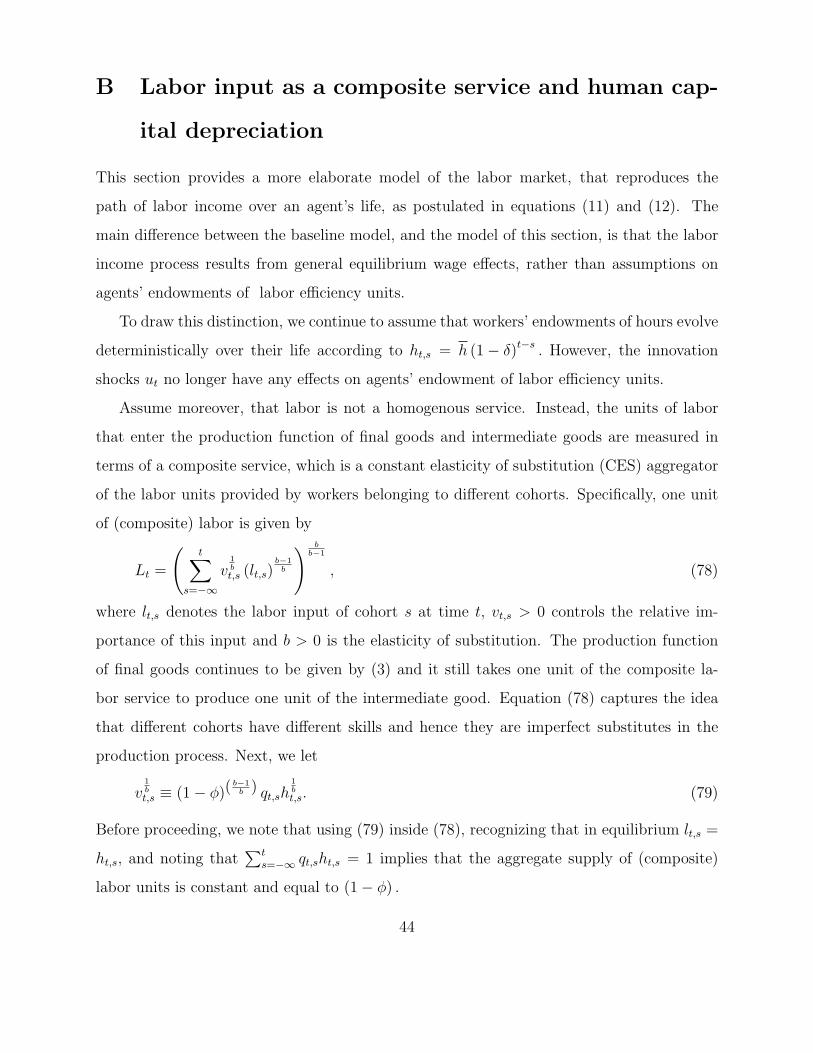
B Labor input as a composite service and human cap-
ital depreciation
This section provides a more elaborate model of the labor market, that reproduces the
path of labor income over an agent’s life, as postulated in equations (11) and (12). The
main difference between the baseline model, and the model of this section, is that the labor
income process results from general equilibrium wage effects, rather than assumptions on
agents’ endowments of labor efficiency units.
To draw this distinction, we continue to assume that workers’ endowments of hours evolve
deterministically over their life according to ht,s = h (1 − δ)t−s . However, the innovation
shocks ut no longer have any effects on agents’ endowment of labor efficiency units.
Assume moreover, that labor is not a homogenous service. Instead, the units of labor
that enter the production function of final goods and intermediate goods are measured in
terms of a composite service, which is a constant elasticity of substitution (CES) aggregator
of the labor units provided by workers belonging to different cohorts. Specifically, one unit
of (composite) labor is given by
Lt =
(t∑
s=−∞v
1bt,s (lt,s)
b−1b
) bb−1
, (78)
where lt,s denotes the labor input of cohort s at time t, vt,s > 0 controls the relative im-
portance of this input and b > 0 is the elasticity of substitution. The production function
of final goods continues to be given by (3) and it still takes one unit of the composite la-
bor service to produce one unit of the intermediate good. Equation (78) captures the idea
that different cohorts have different skills and hence they are imperfect substitutes in the
production process. Next, we let
v1bt,s ≡ (1 − φ)(
b−1b ) qt,sh
1bt,s. (79)
Before proceeding, we note that using (79) inside (78), recognizing that in equilibrium lt,s =
ht,s, and noting that∑t
s=−∞ qt,sht,s = 1 implies that the aggregate supply of (composite)
labor units is constant and equal to (1 − φ) .
44

Since labor inputs by agents belonging to different cohorts are imperfect substitutes, we
need to solve for the equilibrium wage wt,s of each separate cohort. This process is greatly
facilitated by first constructing a “wage index”, i.e. taking a set of cohort-specific wages as
given, and then minimizing (over cohort labor inputs) the cost of obtaining a single unit of
the composite labor input. As is well established in the literature, this wage index for CES
production functions is given by
wt =
(t∑
s=−∞vt,s (wt,s)
1−b) 1
1−b
.
With this wage index at hand, the cohort specific input demands for a firm demanding
a total of Lt units of the composite good are given by
wt,s = wtv1bt,s
(lt,sLt
)− 1b
. (80)
It is now straightforward to verify that an equilibrium in such an extended model can be
determined by setting wt = wt (where wt is given by [24]) and then obtaining the cohort-
specific wages by setting lt,s = ht,s, and Lt = (1 − φ) in equation (80) and solving for wt,s.
To see this, note that by making these substitutions and using (79) inside (80) leads to the
per-worker income process
wt,sht,s(1 − φ)
= wtqt,s , (81)
which coincides with the labor income process in the baseline model. Furthermore by setting
wt = wt, the market for total (composite) labor units clears by construction, whereas the
cohort specific wages implied by (81) clear all cohort specific labor markets, since they satisfy
equation (80) for all markets.
45

C Data Description
The CEX data are from the NBER website as compiled by Ed Harris and John Sabelhaus.
See http://www.nber.org/ces cbo/Cexfam.pdf for a detailed description of the data. In
short, the data set compiles the results from the four consecutive quarterly interviews in the
CEX into one observation for each household. We follow a large literature (see e.g. Vissing-
Jogensen (2002)) and drop from the sample households with incomplete income responses,
households who haven’t completed one of the quarterly interviews, and households that
reside in student housing. To ensure that data selection does not unduly affect the results,
we also ran all the regressions on the raw data including dummies for reporting status and
the number of completed interview quarters. The results were not affected in any essential
way.
A more delicate issue concerns the definition of consumption. As Fernandez-Villaverde
and Krueger (2007), we used a comprehensive measure of consumption that potentially in-
cludes durables. Specifically, we used exactly the same definition as Harris and Sabelhaus.
Our choice is motivated by our model; according to the model, cohort effects are determined
by the intertemporal budget constraint of agents born at different times. Accordingly, as
Fernandez-Villaverde and Krueger (2007), we use total consumption expenditure in the es-
timation of cohort effects. To test if this choice materially affects our results, we also ran
the results using non-durable consumption (total consumption expenditure excluding med-
ical and educational expenses, housing, furniture and automotive related expenses). Using
non-durable consumption the volatility of cohort effects was larger; however, there was not
a big difference between the variance of the permanent components of the cohort effects, no
matter which concept of consumption (total or only non-durable) we used. This is to be
expected, as one would expect the two notions of consumption to share the same permanent
component.
46

References
Abel, A. B. (1990, May 1990). Asset prices under habit formation and catching up with the joneses.
American Economic Review 80 (2), 38–42.
Abel, A. B. (2003, March 2003). The effects of a baby boom on stock prices and capital accumulation
in the presence of social security. Econometrica 71 (2), 551–578.
Barro, R. J. (2006, August 2006). Rare disasters and asset markets in the twentieth century.
Quarterly Journal of Economics 121 (3), 823–66.
Berk, J. B., R. C. Green, and V. Naik (1999). Optimal investment, growth options, and security
returns. Journal of Finance 54 (5), 1553 – 1607.
Beveridge, S. and C. R. Nelson (1981). A new approach to decomposition of economic time series
into permanent and transitory components with particular attention to measurement of the
’business cycle.’. Journal of Monetary Economics 7 (2), 151 – 174.
Blanchard, O. J. (1985, April 1985). Debt, deficits, and finite horizons. Journal of Political
Economy 93 (2), 223–247.
Campbell, J. Y. and J. H. Cochrane (1999, April 1999). By force of habit: A consumption-based
explanation of aggregate stock market behavior. Journal of Political Economy 107 (2), 205–251.
Carlson, M., A. Fisher, and R. Giammarino (2004). Corporate investment and asset price dynamics:
Implications for the cross-section of returns. Journal of Finance 59 (6), 2577 – 2603.
Constantinides, G. M., J. B. Donaldson, and R. Mehra (2002, February 2002). Junior can’t borrow:
A new perspective of the equity premium puzzle. Quarterly Journal of Economics 117 (1), 269–
96.
Deaton, A. and C. Paxson (1994). Intertemporal choice and inequality. Journal of Political Econ-
omy 102 (3), 437–467.
DeMarzo, P. M., R. Kaniel, and I. Kremer (2004). Diversification as a public good: Community
effects in portfolio choice. Journal of Finance 59 (4), 1677 – 1715.
47

Fama, E. F. and K. R. French (1992). The cross-section of expected stock returns. Journal of
Finance 47 (2), 427–65.
Fernandez-Villaverde, J. and D. Krueger (2007). Consumption over the life cycle: Facts from
consumer expenditure survey data. Review of Economics and Statistics 89 (3), 552 – 565.
Garleanu, N. and S. Panageas (2007). Young, old, conservative and bold: The implications of finite
lives and heterogeneity for asset pricing. Working Paper, Wharton and Haas-Berkeley.
Gomes, F. and A. Michaelides (2007). Asset pricing with limited risk sharing and heterogeneous
agents. Forthcoming, Review of Financial Studies.
Gomes, J., L. Kogan, and L. Zhang (2003). Equilibrium cross section of returns. Journal of Political
Economy 111 (4), 693 – 732.
Hubbard, G. R., J. Skinner, and S. P. Zeldes (1994). The importance of precautionary motives
for explaining individual and aggregate saving. Carnegie-Rochester Conference Series on Public
Policy 40, 1–67.
Jones, C. I. (1997). Introduction to Economic Growth (First Edition ed.). New York and London:
W.W. Norton.
Lucas, R. E. (1978, November 1978). Asset prices in an exchange economy. Econometrica 46 (6),
1429–1445.
McKenzie, D. J. (2006). Disentangling age, cohort and time effects in the additive model. Oxford
Bulletin of Economics and Statistics 68 (4), 473 – 495.
Mehra, R. and E. C. Prescott (1985, March 1985). The equity premium: A puzzle. Journal of
Monetary Economics 15 (2), 145–161.
Papanikolaou, D. (2007). Investment-specific shocks and asset prices. Working Paper, Kellogg.
Romer, P. M. (1990, October). Endogenous technological change. Journal of Political Econ-
omy 98 (5), 71–102.
48

Storesletten, K., C. I. Telmer, and A. Yaron (2007). Asset prcing with idiosyncratic risk and
overlapping generations. Review of Economic Dynamics 10 (4), 519–548.
Vissing-Jogensen, A. (2002). Limited asset market participation and the elasticity of intertemporal
substitution. Journal of Political Economy 110 (4), 825 – 853.
Zhang, L. (2005). The value premium. Journal of Finance 60 (1), 67–103.
49