The declining profitability of litchi orchards in northern...
26
1 The declining profitability of litchi orchards in northern Thailand: Can innovations reverse the trend? Pepijn Schreinemachers Dept. of Land Use Economics in the Tropics and Subtropics, Universität Hohenheim, 70593 Stuttgart, Germany ([email protected]) Chakrit Potchanasin Dept. of Agricultural and Resource Economics, Faculty of Economics, Kasetsart University, Bangkok 10900, Thailand ([email protected]) Thomas Berger Dept. of Land Use Economics in the Tropics and Subtropics, Universität Hohenheim, 70593 Stuttgart, Germany ([email protected]) Sithidech Roygrong Institute for Plant Nutrition, Universität Hohenheim, 70593 Stuttgart, Germany ([email protected]) Contributed Paper prepared for presentation at the International Association of Agricultural Economists’ 2009 Conference, Beijing, China, August 16-22, 2009. Copyright 2009 by Pepijn Schreinemachers, Chakrit Potchanasin, Thomas Berger, and Sithidech Roygrong. All rights reserved. Readers may make verbatim copies of this document for non- commercial purposes by any means, provided that this copyright notice appears on all such copies.
Transcript of The declining profitability of litchi orchards in northern...

1
The declining profitability of litchi orchards in northern
Thailand: Can innovations reverse the trend?
Pepijn Schreinemachers Dept. of Land Use Economics in the Tropics and Subtropics, Universität Hohenheim, 70593
Stuttgart, Germany ([email protected])
Chakrit Potchanasin Dept. of Agricultural and Resource Economics, Faculty of Economics, Kasetsart University,
Bangkok 10900, Thailand ([email protected])
Thomas Berger Dept. of Land Use Economics in the Tropics and Subtropics, Universität Hohenheim, 70593
Stuttgart, Germany ([email protected])
Sithidech Roygrong Institute for Plant Nutrition, Universität Hohenheim, 70593 Stuttgart, Germany
Contributed Paper prepared for presentation at the International Association
of Agricultural Economists’ 2009 Conference, Beijing, China, August 16-22, 2009.
Copyright 2009 by Pepijn Schreinemachers, Chakrit Potchanasin, Thomas Berger, and Sithidech
Roygrong. All rights reserved. Readers may make verbatim copies of this document for non-
commercial purposes by any means, provided that this copyright notice appears on all such
copies.

2
The declining profitability of litchi orchards in northern
Thailand: Can innovations reverse the trend?
Abstract
Litchi is an important crop in the mountainous part of northern Thailand yet its profitability has
declined during the last 15 years. The replacement of litchi fruit orchards for seasonal flowers
and vegetables has external costs related to increased levels of erosion, pesticide use, and
irrigation water use. Using a combination of financial analysis and agent-based modeling, the
paper ex-ante assesses the impact of four technologies—artificial flower induction, small-scale
cooperative fruit drying, post-harvest treatments to extend the shelf-life of fresh fruits, and
greater irrigation efficiency—in terms of profits, farm incomes, litchi acreage, erosion, and
pesticide use. The model was calibrated to one watershed in Chiang Mai province where
economic development has been rapid. Although each technology substantially increases the
profitability of litchi growing, scenario analysis shows that this is not enough to stem the decline
in litchi orchards in the study area. To achieve this, the innovations would have to be combined
with an increase in the fresh fruit price at the farm gate from about 9 baht/kg at present to at least
12 baht/kg.
Keywords: ex-ante technology assessment, innovation adoption, agent-based modeling, bio-
economic models
3
Introduction
China, Taiwan, India, Thailand, and Vietnam are the world’s largest producers of litchi (Litchi
chinensis Sonn.). Production in Thailand is concentrated in the northern uplands and is mostly
produced by Thai farmers of Hmong and Karen ethnic origin.1 During the last decade, the area of
litchi orchards has more than doubled in northern Thailand (Office of Agricultural Economics,
2008). Average farmgate prices have, however, declined at the same time (Figure 1). Domestic
overproduction is probably the main cause of this decline and is exacerbated by the fact that the
fruit harvest in northern Thailand is concentrated in only a short period from the end of May till
the end of June.
Low and declining litchi prices have lowered profits to farmers, who in some regions have
reduced orchard management, and in some cases have cut down trees. This trend can be seen as a
logical and perhaps necessary adjustment in response to relative price changes: the litchi area
expands in more remote areas that are opening up to markets (i.e., Withrow-Robinson et al.
1999), while it shrinks in economically well-developed areas with more profitable alternatives.
Yet, the loss of fruit trees in some areas has raised environmental concerns as those more
profitable alternatives, such as flowers and vegetables, could worsen current problems of soil
erosion, rapid runoff and risk of flooding, environmental contamination with pesticides, and loss
of biodiversity.
Responding to these concerns, scientists have been developing technological innovations to
boost the relative profitability of litchi cultivation. The objective of this paper is to ex-ante asses
1 The northern region accounted for 85 percent of the Thai litchi output and 87 percent of the planted area in 2007
(Office of Agricultural Economics, 2008).

4
four of these innovations: off-season fruit production, small-scale cooperative fruit drying,
improved irrigation management, and fruit preservation methods to extent shelf-life. The ex-ante
assessment is performed in terms of profitability, farm household incomes, area under litchi
orchards, irrigation water use, and levels of soil erosion and pesticide use. Profitability is
assessed using a financial analysis of each innovation while the other indicators are assessed at a
farm household and landscape level for which we use an integrated model of one watershed in
northern Thailand. An agent-based modeling approach was selected to capture the heterogeneity
of farm households in terms of opportunity costs and economic constraints.
Figure 1 Farmgate price and planted area of litchi in northern Thailand, 1994-2007
Source: Office of Agricultural Economics, 2008
The paper proceeds in the next section with a description of the four innovations studied. This is
followed by an account of the used methodology. A subsequent section shows the results, after
which we reach a conclusion.
area
price
0
10
20
30
40
50
Pric
e (b
aht/k
g)
0
5
10
15
20
25
Are
a (1
,000
ha)
1994 1996 1998 2000 2002 2004 2006 2008

5
Theoretical background
The cyclical oversupply of agricultural products has been subject of considerable debate in
agricultural economics (Cochrane 2003, Levins and Cochrane 1996, Binswanger and von Braun
1991, Marion and Wills 1990, Cochrane 1985). Technological progress stimulates productivity
growth in agriculture, yet because the demand for primary commodities tends to be inelastic, the
increase in demand does not keep up with the increase in output, thereby creating a downward
pressure on the price. Farmers as a results need to adopt cost-saving or yield increasing
technologies just to stay at the same level of profit. Willard Cochrane theorized this insight in the
1950s when trying to explain why farm incomes in the United States were persistently low in
spite of the rapid technological progress of the time (Cochrane 1958).
Technological innovations that raise crop yields are usually popular with farmers and can bring
short-term profits to those who are relatively quick to adopt. But as the innovation spreads, the
long-run gains will be captured not by farmers in the form of higher profits but by consumers in
the form of lower food prices. From the producer side, it is virtually impossible to organize
producers to collectively control the volume of farm output, as for each individual farmer, the
marginal revenue from selling one more unit of output outweighs the marginal cost of producing
it. Some authors have argued that agricultural oversupply is not necessary a bad thing as
declining food prices benefit consumers and keep the agricultural sector competitive
internationally, while farmers can keep up profits through crop substitution or diversification
(Binswanger and von Braun 1991).
We note that attempts at controlling oversupply, have mostly been through institutional rather
than technological innovations. In European countries governments, for instance, have enacted
quota on dairy production, while in viniculture there is large range of measures including quality
6
control and labeling, yield limits by wine growing associations, bans on new planting of vines,
and government subsidies for grubbing-up existing vineyards. For tropical commodities, price
controls through International Commodity Agreements and government-controlled marketing
boards were common in the 1970s and 80s for coffee, cocoa, rubber, and sugar. These programs
largely disappeared during the 1990s when the focus shifted to economic liberalization and
structural adjustment. Although the innovations studied in this paper are all technological
innovations, none of them aims at increasing litchi yields as such. Yield increasing innovations,
such as planting litchi trees more densely, were not considered in this study.
Proposed agricultural innovations
Scientists from Chiang Mai University and Mae Jo University in Thailand in collaboration with
scientists from Hohenheim University in Germany have been developing four technologies that
could improve the profitability of litchi in northern Thailand. These technologies, shown in
Table 1, are elaborated in the following.
• Artificial flower induction. In 1998, scientists found that the application of potassium
chlororate (KClO3) can artificially induce flowering in longan (Manochai et al. 1999). This
invention allowed farmers to spread the fruit harvest more evenly throughout the year. Litchi
and longan are closely related species and scientists hope to develop a similar method for
artificial flower induction in litchi.
• Small-scale cooperative fruit drying. Litchi fruits must the picked when ripe as the fruit does
not ripen off the tree. Yet farmers cannot store the fresh fruit as it has a vulnerable rind that is
susceptible to decay (Jiang et al. 2006). Farmers must therefore sell the fruits immediately
and have little negotiating power if markets are over-supplied. Drying of fresh litchi fruits in
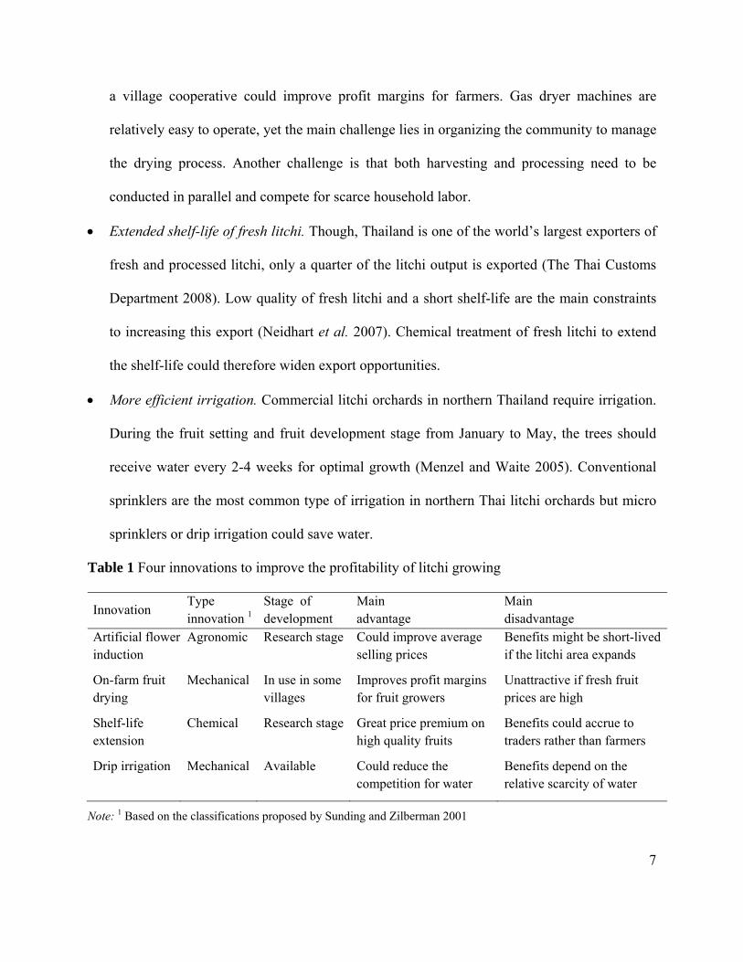
7
a village cooperative could improve profit margins for farmers. Gas dryer machines are
relatively easy to operate, yet the main challenge lies in organizing the community to manage
the drying process. Another challenge is that both harvesting and processing need to be
conducted in parallel and compete for scarce household labor.
• Extended shelf-life of fresh litchi. Though, Thailand is one of the world’s largest exporters of
fresh and processed litchi, only a quarter of the litchi output is exported (The Thai Customs
Department 2008). Low quality of fresh litchi and a short shelf-life are the main constraints
to increasing this export (Neidhart et al. 2007). Chemical treatment of fresh litchi to extend
the shelf-life could therefore widen export opportunities.
• More efficient irrigation. Commercial litchi orchards in northern Thailand require irrigation.
During the fruit setting and fruit development stage from January to May, the trees should
receive water every 2-4 weeks for optimal growth (Menzel and Waite 2005). Conventional
sprinklers are the most common type of irrigation in northern Thai litchi orchards but micro
sprinklers or drip irrigation could save water.
Table 1 Four innovations to improve the profitability of litchi growing
Innovation Type innovation 1
Stage of development
Main advantage
Main disadvantage
Artificial flower induction
Agronomic Research stage Could improve average selling prices
Benefits might be short-lived if the litchi area expands
On-farm fruit drying
Mechanical In use in some villages
Improves profit margins for fruit growers
Unattractive if fresh fruit prices are high
Shelf-life extension
Chemical
Research stage Great price premium on high quality fruits
Benefits could accrue to traders rather than farmers
Drip irrigation Mechanical Available Could reduce the competition for water
Benefits depend on the relative scarcity of water
Note: 1 Based on the classifications proposed by Sunding and Zilberman 2001

8
Methodology
Profitability is a necessary but insufficient condition for farm level adoption. Resource
constraints (land, labor, cash, and water), opportunity costs, and knowledge about the
innovations also affect adoption. Because these aspects vary between farm households as well as
over time, the adoption by farm households is neither instantaneous nor simultaneous. We
therefore used a combination of financial analysis to estimate the profitability of each innovation
and integrated modeling to simulate potential levels of farm level adoption and its economic and
environmental impact in a heterogeneous population of farm households.
In agricultural economics, whole farm programming models are commonly used to identify
possible resource constraints and to ex-ante assess the impact of agricultural innovations. As
these models are linear in the equations, the outcomes tend to be sensitive to small changes in the
resource constraints. Though abrupt changes can be a realistic outcome for technology adoption
at the level of an individual farm, such abrupt changes are only rarely observed at a population
level.
Berger (2001) and Schreinemachers et al. (2007) overcame this drawback of representative MP
models by using an agent-based modeling approach. In such an approach, each real-world farm
household can be individually represented as a computational agent. Though each agent can
experience an abrupt change in its land use, the aggregate response of a heterogeneous
population of agents tends to be smooth. Berger and Schreinemachers (2006) and Robinson et al.
(2007) showed that a population of agents can be statistically estimated from farm household
survey data.
9
This study used an approach called mathematical programming-based multi-agent systems (MP-
MAS). It is a freeware software application developed at Hohenheim University.2 The MP-MAS
software sequentially calibrates an MP tableau to each individual farm household in a population
keeps track of dynamics, and estimates technical coefficients using various biophysical models.
As plot-specific data are organized in spatial layers, the model can be used to analyze spatial
changes in land use and land cover. Table A1 shows a concise outline of the MP tableau. Farm
households were assumed to maximize the expected net farm and non-farm income. Though the
model runs at an annual time step, it includes monthly land, labour, and water constraints to
capture multiple cropping, peak labour needs, and monthly variations in the irrigation water
supply.
The four litchi-related innovations were included as separate activities in the tableau. Each agent
was given an initial amount of litchi orchards corresponding to the observed area in the farm
household survey. The fruit yield depends on the intensity of management and the age of the
orchard. Each orchard was given a random age between 5 and 30 years to initialize the model.
Neef et al. (2000) observed that farmers in the Mae Sa watershed do not normally cut their
orchards, even if unproductive. Most of the agricultural land is located inside the boundaries of
the Doi Suthep-Pui National Park and the land could be claimed by the park authorities if it looks
unused. Keeping the land covered with fruit trees is therefore more secure. The felling of
orchards was therefore not included as an activity in the tableau; only after reaching the
maximum lifespan can an orchard be felled.
2 The software plus user manual can be downloaded from https://mp-mas.uni-hohenheim.de/
10
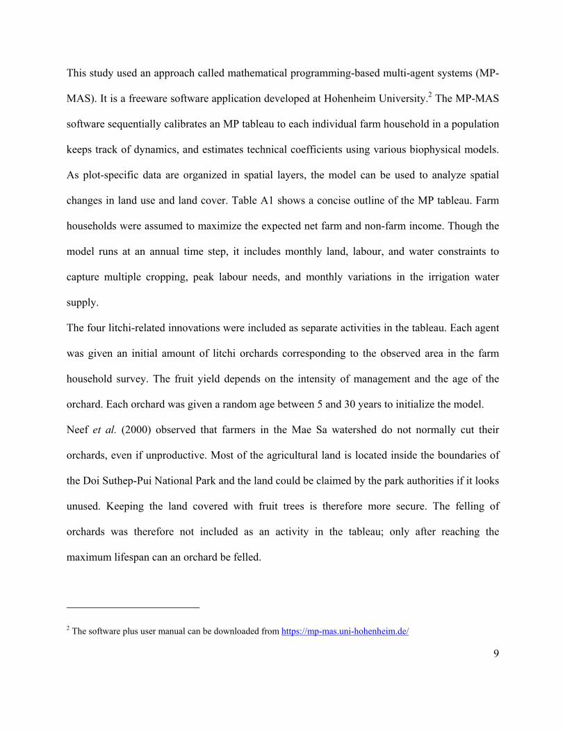
For each year in the simulation, two MP problems were solved for each agent, simulating
investment and production decisions, respectively (Figure 2). Investments included the
acquisition of new technologies and assets, such as the expansion of litchi fruit orchards and the
purchase of a fruit drying machine. For the investment problem, which was solved first at the
beginning of each simulation period, the agent optimized the expected net returns averaged over
the lifespan of each asset, using an annuity cost approach. For the following production problem,
new investments were then added to the available resources of the agent while the purchase price
was subtracted from the agent’s liquidity. This second MP problem optimized the annual
production decision: the allocation of cash, land, labour, and water to a monthly cropping plan
(Schreinemachers and Berger, 2006). Although the model integrated various biophysical aspects
such as pesticide toxicity, soil loss, and precipitation, it did not include any feedback effects in
the biophysical system.
Figure 2 Dynamics of the agent-based decision model
Biophysical components
Economic components
Investment decisions
Production decisions
Soil erosion
Pesticide use
Net incomes
Crop yields
Rainfall + inflows
Water use
Updating of expectations & liquidity
Updating of
liquidity & assets
11
A balance equation was used to update the amount of liquid means (LIQ) between periods:
(1)
in which the household revenues (REV) minus the variable costs (VAR) minus the investment
costs (FIX) equals the total gross margin of the MP matrix.3 The profit that is not consumed
(CONS) and is not used to repay loans (DEBT), is then added to the liquid means and is
available to farm production in the next period.
Agents used adaptive expectations for investment and production decisions; this implies that the
agents formed expectations about what will happen in the future based on what happened in the
past. Following the implementation of adaptive expectations of Berger (2001), agents revise their
expectations in each period in proportion to the difference between actual (Xt-1) and expected
values (X*t-1) as:
, 0 1, (2)
in which λ is the coefficient of expectations. This model of expectation formation is applied to
prices, water supply, and crop yields. The assumption of adaptive expectations is only realistic if
there is no systematic trend, as real farm household would otherwise develop foresight. After
agents decided on investment and production, the solution vector of the MP matrix was
recalculated for each agent using actual values.
3 Note that the amount of cash not used for investments (FIX) or the purchase of variable inputs (VAR) equals the
amount of short-term deposits (DEP): . Another way of writing equation (2) is
therefore: , that is liquid means at the end of the period equals deposits
plus new savings.

12
Crop yields were modeled following the FAO CropWat model (Smith 1992, Clarke et al. 1998).
The crop-water requirement (CWR) for crop c in month m is the product of a crop coefficient
(KC), the potential evapotranspiration (ETO), and the planted area (Area):
CWRcm = KCcm* ETOm * Areacm (3)
The CWR could either be met through irrigation (IRR) or rainfall, which was converted into
effective rainfall (ER) to capture the share of rainfall actually available to the crop, depending on
its growth stage. The amount of water actually supplied (CWS) was then as follows:
CWScm = ERcm + IRRcm (4)
For lack of detailed data from the study region, the quotient of crop water supplied and the crop
water requirement were simply averaged over all months with non-zero crop water requirements:
Krc = (1/m * ∑(CWScm / CWRcm) | CWRcm > 0) (5)
The crop growth model assumed that the crop yield was lost if the average Kr fell below 0.5,
while for Kr values greater than or equal to 0.5 the Kr value was multiplied by the crop yield
potential (YPOT) to simulate the actual crop yield (Yc):
(6)
Rainfall, groundwater, and surface water were the sources of crop water supply in the model.
Daily rainfall data were generated following Yaoming et al. (2004). Agents, as their real-world
analogues, derived irrigation water from either groundwater or streams (surface water).
Groundwater was assumed to give an unlimited water supply but only to those agents that had
already access (about 11 percent in the central valley, as identified from the survey). Surface
water needed to be shared among agents in the same village. The irrigation water supply (IRR)
Yc =
Krc * YPOTc if Krc ≥ 0.5
0 if Krc < 0.5
13
was approximated using a backward calculation on observed pattern of land use, irrigation
methods, irrigation sources, and effective rainfall. Let IEFFjck be the efficiency of irrigation
method j used on crop c by a household k. The irrigation water use of household k was then
calculated by summing the irrigation water use over all months and crops as:
∑ ∑ CWR (7)
in which GR was the groundwater use. The sum over all households in an area that shared a
common water source thereby approximated the total volume of the surface water for irrigation.
Outcome indicators
Four outcome indicators were used to analyze the simulation results:
• Area under litchi fruit orchards, an increase of which is the basic objective of the proposed
innovations.
• Net farm household incomes, calculated as the sum of farm and non-farm income.
• Pesticide loads were quantified using the Environmental Impact Quotient (EIQ) method
(Kovach et al. 2008). Following this method, an average field use rating, which was a
proxy for toxicity, was calculated for each crop.
• Erosion soil loss was quantified using the Revised Universal Soil Loss Equation (RUSLE)
in which the amount of soil loss is a function of the steepness and length of the slopes,
rainfall erosivity, soil erodibility, crop choice and crop management, and erosion control
measures.
Study area and data collection
The study was conducted in the Mae Sa watershed area. This watershed, 140 km2 in size that lies
about 40 km northwest of Chiang Mai city, has an elevation ranging from 300 to 1700 meters
14
a.s.l. There are an estimated 1,309 farm households with a permanent residence in the watershed
and 313 of these grow litchi (24 percent). Most of the litchi is grown in the upper parts of the
watershed at elevations above 1000 meters by Thai citizens of Hmong ethnic origin. In the seven
Hmong villages in the watershed, 39 percent of the agricultural land area is occupied by litchi
trees.
Because of the proximity of the watershed to Chiang Mai city and other urbanized areas, the
opportunity costs to litchi growing are high. Especially with low litchi prices, many households
choose not to manage their litchis but to perform non-farm work or intensify field crop
production, sometimes by cutting down orchards. The main alternative crops for upland farmers
are cabbage, potato, carrot and cut flowers like rose and gerbera. The research area is therefore
not representative for agricultural in northern Thailand, yet if the study would show that the
innovations make litchi growing competitive in the Mae Sa watershed then it would certainly be
competitive in most of northern Thailand.
Data about each of the four innovations were collected from secondary sources, such as
publications, and through interviews with scientists developing these technologies. As some
technologies are not available at this moment, the financial assessment uses assumptions on the
costs and benefits and tests the results for alternative assumptions. To calibrate the land use
model, farm household data were collected using a structured questionnaire survey on a random
sample of 303 farm households from October to November 2006. Secondary data were used in
addition to calibrate the model, such as crop water requirements and precipitation data. All
pesticides used in the watershed were converted to EIQ values based on their active ingredients
and application rates.

15
Results
Average profitability of litchi growing in the Mae Sa watershed
Average fruit yields of litchi orchards in the Mae Sa watershed area are about 3.1 tons/ha. At an
average selling price of 9 baht per kilogram this creates revenues of about 28 thousand baht/ha.
Since the variable input use is relatively low, the profitability of litchi is mostly a function of the
price of fresh litchi and the valuation of labor, as shown in Figure 3. At a current wage rate of
100-140 baht per man-day and a litchi price varying between 6 and 12 baht/kg, profits range
from -7 to 15 thousand baht/ha. At an average wage rate of 120 baht, the break-even-point for
litchi growing is 7.7 baht/kg.
Figure 3 Profitability of litchi growing by levels of selling price and wage rate
Source: Own estimates from 2006 farm household survey
Note: The rectangle indicates the current range of profits
Profit level:[1,000 baht/ha]
0
20
40
60
80
100
120
140
160
Pric
e of
labo
r (ba
ht/m
an-d
ay)
0 2 4 6 8 10 12 14 16
Farmgate price of fresh litchi (baht/kg)
< -10
-10 to 0
0 to 10
10 to 20
> 20
16
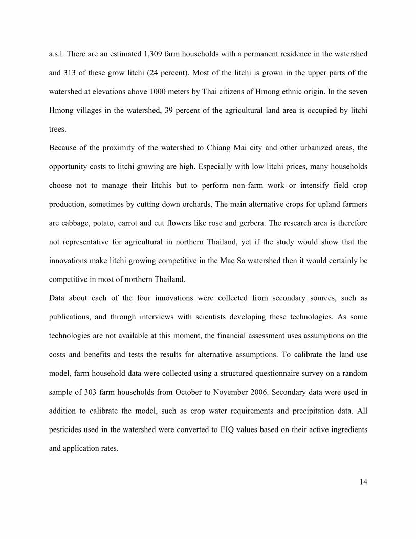
Figure 4 compares the profitability of litchi and off-season litchi with that of various other crops
grown in the watershed, excluding the cost of labor, water, and land. Because of the great
differences in altitudes within the study area, not all crops are substitutes. Though, the graph
might suggest a certain pessimism about litchi growing in the watershed, whether farm
households will grow it not only depends on the relative profitability but also on land, labor,
water and cash constraints which are scrutinized in the integrated analysis.
Figure 4 Profitability of litchi compared to other crops
Note: Calculations excludes all labor costs and the cost of irrigation infrastructure except for bell pepper.
Average profitability of the innovations
The costs and returns of artificial flower induction were based on the experience in off-season
longan production. Artificial flower induction in longan has been widely adopted since its
0100200300400500
Profit margin (1000 baht/ha)
Bell pepperRoseStrawberryChrysanthemumGerberaOnionWhite cabbagePotatoBaby carrotBrocoliChayoteLitchi (off-season)Chinese cabbageCarrotLitchi (in-season)LettuceString/Bush beanLonganPaddy riceGingerSoybeanSweetcornChinese kaleWhite radishFeed maize

17
introduction in 1998, during the so-called “longan mania” the planted area increased 7 percent
annually from 1998 to 2007. Figure 5 shows the average monthly price for longan fruits. The
average in-season fruit price from July to August was 12.3 baht/kg (sd=5.6) while the average
off-season price was 21.7 baht/kg (sd=6.1), which suggests an average premium of about 9.4
baht/kg (76 percent) yet average fresh fruit prices declined during this period. Based this
experience, a price premium of 40-60 percent can be expected for off-season litchi. At a fruit
price of 9 baht/kg and an average labor price of 120 baht/man-day, this would translate into an
average increase in profits from about 7.57 thousand baht/ha for in-season harvesting to 21.06
thousand baht/ha for off-season harvesting (Table 2).
Figure 5 Average monthly farmgate price of longan in northern Thailand, 2001-2008
Source: Office of Agricultural Economics, 2008
The break-even-point of litchi dryer was estimated to lie at a fresh fruit price of 8.24 baht/kg. At
fresh fruit price above this price, selling the fresh fruits brings a greater profit then drying.
Because fruit drying is labor intensive, the profits are substantially higher if own household labor
is not accounted for. Excluding own labor costs, the fruit drying is attractive also at higher fresh
0
10
20
30
40
50
Pric
e (b
aht/k
g)
1 2 3 4 5 6 7 8 9 10 11 12
AverageStandard deviation95% Confidence interval
18
fruit prices. The possibility of compensating low litchi prices with fruit drying is an attractive
option as it increases profits but does not increase the fresh fruit supply and does therefore not
suppress fresh litchi prices.
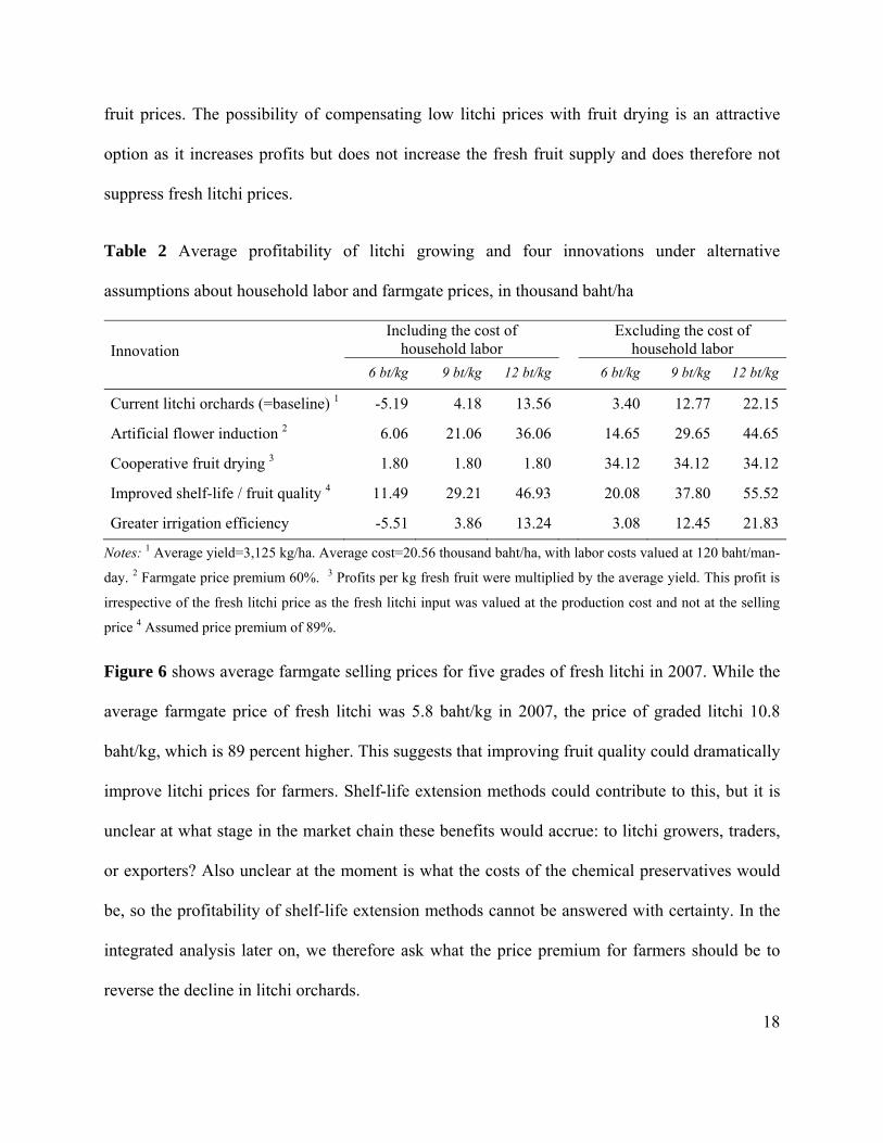
Table 2 Average profitability of litchi growing and four innovations under alternative
assumptions about household labor and farmgate prices, in thousand baht/ha
Innovation Including the cost of
household labor Excluding the cost of household labor
6 bt/kg 9 bt/kg 12 bt/kg 6 bt/kg 9 bt/kg 12 bt/kg
Current litchi orchards (=baseline) 1 -5.19 4.18 13.56 3.40 12.77 22.15
Artificial flower induction 2 6.06 21.06 36.06 14.65 29.65 44.65
Cooperative fruit drying 3 1.80 1.80 1.80 34.12 34.12 34.12
Improved shelf-life / fruit quality 4 11.49 29.21 46.93 20.08 37.80 55.52
Greater irrigation efficiency -5.51 3.86 13.24 3.08 12.45 21.83
Notes: 1 Average yield=3,125 kg/ha. Average cost=20.56 thousand baht/ha, with labor costs valued at 120 baht/man-
day. 2 Farmgate price premium 60%. 3 Profits per kg fresh fruit were multiplied by the average yield. This profit is
irrespective of the fresh litchi price as the fresh litchi input was valued at the production cost and not at the selling
price 4 Assumed price premium of 89%.
Figure 6 shows average farmgate selling prices for five grades of fresh litchi in 2007. While the
average farmgate price of fresh litchi was 5.8 baht/kg in 2007, the price of graded litchi 10.8
baht/kg, which is 89 percent higher. This suggests that improving fruit quality could dramatically
improve litchi prices for farmers. Shelf-life extension methods could contribute to this, but it is
unclear at what stage in the market chain these benefits would accrue: to litchi growers, traders,
or exporters? Also unclear at the moment is what the costs of the chemical preservatives would
be, so the profitability of shelf-life extension methods cannot be answered with certainty. In the
integrated analysis later on, we therefore ask what the price premium for farmers should be to
reverse the decline in litchi orchards.

19
Figure 6 Farm gate litchi price by grade, 2007
Source: Office of Agricultural Economics, 2008
The irrigation efficiency of sprinklers is about 70 percent, while that of micro sprinklers is about
80 percent. Although the price of a micro sprinkler head is about double that of a conventional
sprinkler head, the main cost of the irrigation infrastructure is PVC pipes rather than sprinkler
heads. As a result, the total per hectare cost of micro sprinklers is only about 4 percent greater
than for conventional sprinkler. As irrigation water has no direct cost, the attractiveness of micro
sprinklers depends on the relative scarcity of this resource.
In summary, the results of the financial analysis showed that the profitability of the innovations
crucially depends not only on the fresh fruit prices but also on the valuation of household labor
and irrigation water. These resources have no direct monetary cost but have a scarcity value and
an opportunity cost that varies between households. To include these in the analysis, we turn to
the integrated assessment.
0 2 4 6 8 10 12 14 16
baht/kg
No grade
Grade 4
Grade 3
Grade 2
Grade 1
20
Results of the integrated assessment
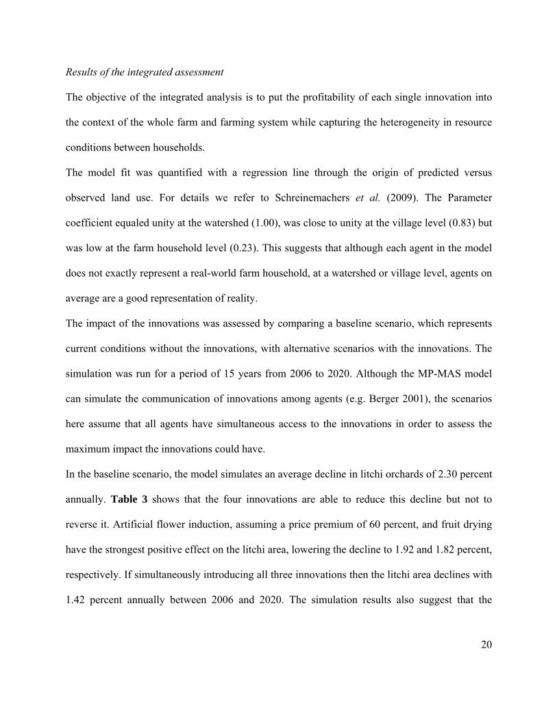
The objective of the integrated analysis is to put the profitability of each single innovation into
the context of the whole farm and farming system while capturing the heterogeneity in resource
conditions between households.
The model fit was quantified with a regression line through the origin of predicted versus
observed land use. For details we refer to Schreinemachers et al. (2009). The Parameter
coefficient equaled unity at the watershed (1.00), was close to unity at the village level (0.83) but
was low at the farm household level (0.23). This suggests that although each agent in the model
does not exactly represent a real-world farm household, at a watershed or village level, agents on
average are a good representation of reality.
The impact of the innovations was assessed by comparing a baseline scenario, which represents
current conditions without the innovations, with alternative scenarios with the innovations. The
simulation was run for a period of 15 years from 2006 to 2020. Although the MP-MAS model
can simulate the communication of innovations among agents (e.g. Berger 2001), the scenarios
here assume that all agents have simultaneous access to the innovations in order to assess the
maximum impact the innovations could have.
In the baseline scenario, the model simulates an average decline in litchi orchards of 2.30 percent
annually. Table 3 shows that the four innovations are able to reduce this decline but not to
reverse it. Artificial flower induction, assuming a price premium of 60 percent, and fruit drying
have the strongest positive effect on the litchi area, lowering the decline to 1.92 and 1.82 percent,
respectively. If simultaneously introducing all three innovations then the litchi area declines with
1.42 percent annually between 2006 and 2020. The simulation results also suggest that the
21
innovations would have a positive but small effect on pesticide loads and soil erosion in the
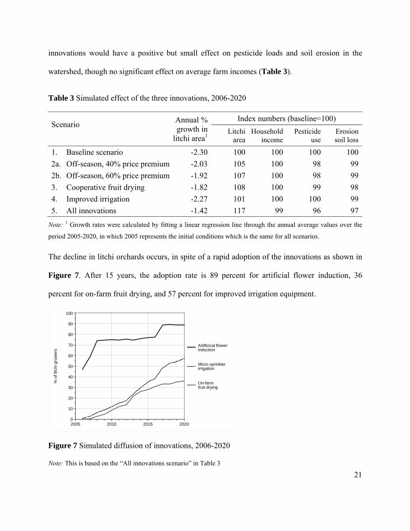
watershed, though no significant effect on average farm incomes (Table 3).
Table 3 Simulated effect of the three innovations, 2006-2020
Scenario Annual % growth in
litchi area1
Index numbers (baseline=100) Litchi
areaHousehold
incomePesticide
use Erosion soil loss
1. Baseline scenario -2.30 100 100 100 1002a. Off-season, 40% price premium -2.03 105 100 98 992b. Off-season, 60% price premium -1.92 107 100 98 993. Cooperative fruit drying -1.82 108 100 99 984. Improved irrigation -2.27 101 100 100 995. All innovations -1.42 117 99 96 97
Note: 1 Growth rates were calculated by fitting a linear regression line through the annual average values over the
period 2005-2020, in which 2005 represents the initial conditions which is the same for all scenarios.
The decline in litchi orchards occurs, in spite of a rapid adoption of the innovations as shown in
Figure 7. After 15 years, the adoption rate is 89 percent for artificial flower induction, 36
percent for on-farm fruit drying, and 57 percent for improved irrigation equipment.
Figure 7 Simulated diffusion of innovations, 2006-2020
Note: This is based on the “All innovations scenario” in Table 3
0
10
20
30
40
50
60
70
80
90
100
% o
f litc
hi g
row
ers
2005 2010 2015 2020
Artificical flowerinduction
Micro sprinklerirrigation
On-farmfruit drying

22
Table 4 Results for alternative fresh fruit prices, with and without innovations, average values
2006-2020 expressed as index numbers (baseline scenario=100).
Fresh litchi price
Litchi orchard area
Household income
Pesticide loads
Erosion soil loss
with without with without with without with without
6 bt/kg 98 94 100 100 100 101 101 1019 bt/kg 106 100* 100 100* 97 100* 98 100*12 bt/kg 124 111 99 99 94 98 94 9715 bt/kg 140 122 98 98 90 94 89 9218 bt/kg 148 132 101 98 86 92 87 8921 bt/kg 153 139 104 99 85 90 86 8624 bt/kg 156 145 108 102 84 89 85 85
Note: * Baseline scenario (same as in Table 4).
The impact of innovations to improve the fresh fruit quality could not be assessed because of
uncertainty about the costs and benefits at the farm level. We therefore analyzed what level of
fresh litchi prices would be needed to reverse the decline in litchi orchards. Fourteen scenarios
were analyzed to answer this question with fresh fruit prices ranging from 6 to 24 baht per
kilogram, as shown in Table 4 and Figure 8. Without innovations, the area stabilizes at about 15
baht/kg, but if all innovations would be available then there would be a moderate growth in litchi
orchards at a price of 12 baht/kg. As it takes about five years for newly planted litchi trees to
give a first fruit yield, the effect on current incomes is small; yet the effect of higher prices on
pesticide use and soil erosion would be substantial.

23
Figure 8 Simulated area under litchi orchards under alternative price scenarios, index 2005=100
Conclusion
Artificial flower induction, on-farm fruit drying, and methods to extend the shelf-life of fresh
fruits increase the profitability of litchi growing, which is currently low, ranging from -7 to 15
thousand baht/ha. The profitability is, however, sensitive to the price of water, household labor,
and land which have no direct monetary cost but only have an opportunity cost. The profitability
of the innovations is a necessary but an insufficient condition for stemming the decline in litchi
orchards. Simulation results of the agent-based watershed model showed rapid adoption rates of
the innovation but no reversal in the downward trend in litchi areas. The results furthermore
showed that the innovations would yield a moderate reduction in the growth of pesticide use and
erosion soil loss. To reverse the decline of litchi orchards, the innovations would have to be
combined with a fresh fruit price of at least 12 baht/kg.
60
70
80
90
100
110
120
130
140
150
160
170In
dex
litch
i are
a
2005 2010 2015 2020
24 bt/kg
21 bt/kg
18 bt/kg
15 bt/kg
12 bt/kg
9 bt/kg
6 bt/kg
Without innovations
60
70
80
90
100
110
120
130
140
150
160
170
Inde
x lit
chi a
rea
2005 2010 2015 2020
24 bt/kg
21 bt/kg
18 bt/kg
15 bt/kg
12 bt/kg
9 bt/kg
6 bt/kg
With innovations

24
Acknowledgement
The financial support of the Deutsche Forschungs Gemeinschaft (DFG) under SFB564 is
gratefully acknowledged. We thank Andreas Neef, Cindy Hugenschmidt, Walaya Sangchang and
other colleagues in the Uplands Program for sharing data and for their helpful discussions.
References
Berger, T., 2001. Agent-based models applied to agriculture: a simulation tool for technology diffusion, resource use changes and policy analysis. Agricultural Economics. 25(2/3), 245-260.
Berger, T., Schreinemachers, P., 2006. Creating agents and landscapes for multiagent systems from random samples. Ecology and Society. 11(2), Art.19.
Binswanger, H., von Braun, J., 1991. Technological change and commercialization in agriculture. The effect on the poor. The World Bank Research Observer. 6(1), 57-80.
Cochrane, W., 1958. Farm prices. Myth and reality., University of Minnesota Press., Minneapolis.
Cochrane, W., 1985. The need to rethink agricultural policy in general and to perform some radical surgery on commodity programs in particular. American Journal of Agricultural Economics. 67(5), 1002-1009.
Cochrane, W., 2003. The curse of American agricultural abundance: a sustainable solution. University of Nebraska Press, Lincoln, NE.
Jiang, Y.M., Wang, Y., Song, L., Liu, H., Lichter, A., Kerdchoechuen, O., Joyce, D.C., Shi, J., 2006. Postharvest characteristics and handling of litchi fruit - An overview. Australian Journal of Experimental Agriculture. 46(12), 1541-1556.
Kovach, J., Petzoldt, C., Degni, J., Tette, J. (2008) A Method to Measure the Environmental Impact of Pesticides. Cornell University, New York State Agricultural Experiment Station Geneva, New York
Levins, R.A., Cochrane, W.W., 1996. The treadmill revisited. Land Economics. 72(4), 550-553. Manochai, P., Suthon, W., Wiriya-alongkom, W., S, S.U., Jarassamrit, N., 1999. Effect of
potassium chlorate on flowering of longan (Dimocarpus longan Lour.) cv. E-daw and Sri-Chompoo (in Thai). Seminar Report on Plant Regulators, Off Season Crop Production. National Research Council of Thailand, Bangkok. p.1-8.
Marion, B.W., Wills, R.L., 1990. A prospective assessment of the impacts of Bovine Somathotropin: A case study of Wisconsin. American Journal of Agricultural Economics. 72(2), 326-336.
Menzel, C., Waite, G.K., 2005. Litchi and Longan: Botany, Production and Uses, in: Menzel, C.M. and Waite, G.K., eds., Litchi and longan: Botany, production and uses, CABI, Wallingford, UK.
Neef, A., Sangkapitux, C., Kirchmann, K., 2000. Does land tenure security enhance sustainable land management? Evidence from mountainous regions of Thailand and Vietnam.

25
Institute of Agricultural Economics and Social Sciences in the Tropics and Subtropics, University of Hohenheim., Discussion Paper No. 2000/2. Stuttgart.
Neidhart, S., Hutasingh, P., Carle, R., 2007. Innovative strategies for sustainable lychee processing, in: Heidhues, F.J., Herrmann, L., Neef, A., Neidhart, S., Pape, J., Sruamsiri, P., Thu, D.C. and Zárate, A.V., eds., Sustainable land use in mountainous regions of Southeast Asia: Meeting the challenges of ecological, socio economic and cultural diversity, Springer-Verlag, Berlin, Heidelberg, New York, London, Paris and Tokyo.
Robinson, D.T., Brown, D.G., Parker, D.C., Schreinemachers, P., Janssen, M., Huigen, M., Wittmer, H., Gotts, N., Promburom, P., Irwin, E., Berger, T., Gatzweiler, F., Barnaud, C., 2007. Comparison of empirical methods for building agent-based models in land use science. Journal of Land Use Science. 2(1), 31-55.
Schreinemachers, P., Berger, T., Aune, J.B., 2007. Simulating soil fertility and poverty dynamics in Uganda: A bio-economic multi-agent systems approach. Ecological Economics. 64(2), 387-401.
Schreinemachers, P., Berger, T., Sirijinda, A., Praneetvatakul, S., 2009. The diffusion of greenhouse agriculture in northern Thailand: Combining econometrics and agent-based modeling, Contributed paper at the International Association of Agricultural Economists' conference, Beijing, August 16-22, 2009.
Sunding, D., Zilberman, D., 2001. The agricultural innovation process: Research and technology adoption in a changing agricultural sector, in: Gardner, B. and Rausser., G.C., eds., Handbook of Agricultural and Resource Economics, Elsevier Science, Amsterdam.
The Thai Customs Department, 2008. Import and export statistics. Accessed available at http://www.customs.go.th/Customs-Eng/Statistic/Statistic.jsp?menuNme=Statistic.
Withrow-Robinson, B., Hibbs, D.E., Gypmantasiri, P., Thomas, D., 1999. A preliminary classification of fruit-based agroforestry in a highland area of northern Thailand. Agroforestry Systems. 42, 195-205.
Yaoming, L.O., Qiang, Z., Deliang, C., 2004. Stochastic modeling of daily precipitation in China. Journal of Geographical Sciences. 14(4), 417-426.

26
Table A1 Part of the MP model showing the decision-making about litchi-related activities in simplified matrix format
Constraint
Annuals (ha) Invest in fruit dryer
Invest/produce litchi (ha) Hire labor in/out
Sell crops (kg)
Dry litchi (kg) Sell litchi (kg) Buy inputs (baht)
Right-hand- side
Rain-fed
Irri-gated
high input
low input
h. input + drip
h. input + off-season
h. input + drip + off.
in season
off-season
in season
off-season
Objective function -C ±E(C) +E(C) +E(C) +E(C) +E(C) +E(C) -E(C)
Resources (monthly) Land (ha) +1 +1 +1 (+1) ≤ (R)Labor (man-days) +A +A (+A) (+A) (+A) (+A) (+A) ±1 (+A) (+A) ≤ (R)Sprinkler irr. (lit/sec) +A +A +A +A ≤ (R)Drip irr. (lit/sec) (+1) +A +A ≤ (R)Resources (annual) Cash (baht), annual +1 ≤ (R)Variable inputs (baht) +A +A (+A) (+A) (+A) (+A) (+A) (+A) -1 ≤ 0 Fruit dryer capacity -A +1 +1 ≤ (R)Litchi orchards (ha) ±1 ±1 ±1 ±1 ±1 ≤ (R)Crop yields (tons) Annual crops E(-Y) E(-Y) +1 ≤ 0 Litchi in-season E(-Y) E(-Y) E(-Y) +1 +1 ≤ 0 Litchi off-season E(-Y) E(-Y) +1 +1 ≤ 0
Notes: C=Price coefficients, A=Technical coefficients, Y=Crop yields, R=Available resources, I=Available innovations, E=Expected values. Values in brackets are adjusted inside the model, of which values in bold are agent-specific.