The DAMBE Manual - XiaLabdambe.bio.uottawa.ca/software_download/LabManualDAMBE.pdfThe DAMBE Manual...
119
The DAMBE Manual Xuhua Xia, 2014
Transcript of The DAMBE Manual - XiaLabdambe.bio.uottawa.ca/software_download/LabManualDAMBE.pdfThe DAMBE Manual...
The DAMBE Manual
Xuhua Xia, 2014

2
CONTENTS
The DAMBE Manual....................................................................................................................................... 1
Instruction for students ................................................................................................................................... 5 Why bioinformatics? .................................................................................................................................... 5 Why DAMBE? ............................................................................................................................................. 5 Be mentally prepared ................................................................................................................................... 5 Know the answers to all questions at end of each lab .................................................................................. 6 My office door is almost always open .......................................................................................................... 6 Acknowledgement ........................................................................................................................................ 6
Lab 1 sequence databases and string matchings ........................................................................................... 7 Summary ...................................................................................................................................................... 7 Data resource and software tools.................................................................................................................. 7
Representative database and web interface: NCBI, GenBank, and Entrez .............................................. 7 Annotated sequences ............................................................................................................................... 8 Sequence formats ..................................................................................................................................... 8 Why do we need to extract sequence elements? ...................................................................................... 9
Retrieve the KAL153 genome with Entrez ................................................................................................ 10 Computing CAI .......................................................................................................................................... 10
Extracting coding sequences from a GenBank file ................................................................................ 10 Computing CAI ..................................................................................................................................... 11
Which subtype does KAL153 belong to? Is it recombinant? ..................................................................... 12 Subtypes in HIV-1 M group .................................................................................................................. 12 Retrieve reference subtype sequences ................................................................................................... 12 Use BLAST to identify subtypes ........................................................................................................... 13
Lecture questions: ...................................................................................................................................... 15 Lab questions: ............................................................................................................................................ 15
Lab 2 Making sense of genomes: Position Weight Matrix (PWM) ........................................................... 16 Introduction ................................................................................................................................................ 16
Two approaches to understand the meaning of a nucleotide sequence .................................................. 16 Extraction of annotated gene features from GenBank files ................................................................... 16 Position weight matrix ........................................................................................................................... 17
Objectives ................................................................................................................................................... 17 Procedures .................................................................................................................................................. 17
A brief peek into a GenBank file ........................................................................................................... 17 Extracting annotated sequence elements with DAMBE ........................................................................ 18 Characterize 5’ and 3’ splice sites with position weight matrix (PWM) ............................................... 18 Scan sequences for splice site signals .................................................................................................... 22 Limitations of PWM .............................................................................................................................. 22
More questions ........................................................................................................................................... 23
Lab 3 Gibbs Sampler and Yeast Intron Properties .................................................................................... 24 Introduction ................................................................................................................................................ 24
Genetic switches .................................................................................................................................... 24 Gibbs sampler and its application in molecular biology ........................................................................ 24 Identifying genetic motifs with Gibbs sampler ...................................................................................... 24
Objectives ................................................................................................................................................... 25 Procedures .................................................................................................................................................. 26
Copy column-based output from DAMBE to EXCEL .......................................................................... 26 Running Gibbs sampler in DAMBE ...................................................................................................... 27 Studying S1 and S2 distances ................................................................................................................ 29
More questions ........................................................................................................................................... 30
3
Lab 5 Codon Usage Bias ................................................................................................................................ 32 Introduction ................................................................................................................................................ 32
Codon usage bias ................................................................................................................................... 32 Codon usage bias and tRNA abundance ................................................................................................ 36
Objectives ................................................................................................................................................... 37 Use RSCU and CAI to characterize codon usage .................................................................................. 37 Understand the relationship between tRNA abundance and codon usage ............................................. 37
Procedures .................................................................................................................................................. 37 Computing CAI and RSCU ................................................................................................................... 37 Identifying tRNA anticodon .................................................................................................................. 41
More questions ........................................................................................................................................... 42
Lab 6 RNA secondary structure, minimum folding energy, and IRES..................................................... 44 Introduction ................................................................................................................................................ 44
RNA secondary structure ....................................................................................................................... 44 Minimum folding energy (MFE) ........................................................................................................... 44 5’ UTR secondary structure and translation economy ........................................................................... 44 Internal ribosomal entry site .................................................................................................................. 45
Objectives ................................................................................................................................................... 45 Procedures .................................................................................................................................................. 45 Assignment ................................................................................................................................................. 46
Lab 7 Protein isoelectric point and acid-resistance ..................................................................................... 47 Introduction ................................................................................................................................................ 47
Protein isoelectric point ......................................................................................................................... 47 Acid-resistance in Helicobacter pylori and its protein isoelectric point ................................................ 47
Objectives ................................................................................................................................................... 49 Compare pI profiles between Escherichia coli and H. pylori ................................................................ 49 Learn to appreciate natural selection and adaptation ............................................................................. 50
Procedures .................................................................................................................................................. 50 Comparison in pI profile between E. coli and H. pylori ........................................................................ 50 Testing evolutionary hypotheses ............................................................................................................ 51
More questions ........................................................................................................................................... 51
Lab 8 Sequence Alignment ............................................................................................................................ 52 Introduction ................................................................................................................................................ 52 Objectives ................................................................................................................................................... 53
How to align homologous nucleotide and amino acid sequences .......................................................... 53 Align protein-coding nucleotide sequences against aligned amino acid sequences ............................... 53 A preview of building phylogenetic trees using aligned sequences ....................................................... 53
Procedures .................................................................................................................................................. 53 Align nucleotide and amino acid sequences .......................................................................................... 54 Align protein-coding nucleotide sequences against aligned amino acid sequences ............................... 56 A preview of molecular phylogenetics .................................................................................................. 56
More questions ........................................................................................................................................... 58
Lab 9 Choosing the best-fit substitution model ........................................................................................... 59 Introduction ................................................................................................................................................ 59 Objectives ................................................................................................................................................... 62
Gain familiarity with the assumptions of nucleotide-based substitution models ................................... 62 Develop skills to choose appropriate substitution models for molecular phylogenetic studies ............. 62 Apply the skill learned to practical phylogenetic analysis ..................................................................... 62
Procedures .................................................................................................................................................. 63 The empirical approach ......................................................................................................................... 63 The statistical model-testing approach ................................................................................................... 72
More questions ........................................................................................................................................... 74
4
Lab 10 Molecular Phylogenetics ................................................................................................................... 75 Introduction ................................................................................................................................................ 75
Major categories of phylogenetic methods ............................................................................................ 75 The plethora of sequence formats for phylogenetic analysis ................................................................. 75 Phylogenetic methods we will learn in this lab ..................................................................................... 76 Distance-based methods ........................................................................................................................ 76 The maximum parsimony (MP) method ................................................................................................ 76 The maximum likelihood (ML) method ................................................................................................ 77 Bootstrapping and jackknifing ............................................................................................................... 77 Phylogenetic reconstruction with a global molecular clock .................................................................. 78
Objectives ................................................................................................................................................... 78 Distance-based, MP and ML methods ................................................................................................... 78 Bootstrap/ jackknife to evaluate subtree reliability ................................................................................ 78 Phylogenetics assuming a global molecular clock ................................................................................. 78
Procedures .................................................................................................................................................. 78 Distance-based method .......................................................................................................................... 79 Maximum parsimony (MP) method ...................................................................................................... 81 Maximum likelihood (ML) reconstruction with bootstrap/jackknife .................................................... 82 Work with the VertCytB.FAS file ......................................................................................................... 83
More questions ........................................................................................................................................... 84
Lab 11 testing the molecular clock hypotheses............................................................................................ 86 Introduction ................................................................................................................................................ 86
Mutation and substitution ...................................................................................................................... 86 The molecular clock hypothesis ............................................................................................................ 86 Statistical tests of the molecular clock hypothesis ................................................................................. 87
Objectives ................................................................................................................................................... 91 Procedures .................................................................................................................................................. 91
Relative-rate tests .................................................................................................................................. 92 Phylogeny-based tests ............................................................................................................................ 93 Do functionally unconstrained sites evolve more clock-like than functionally constrained sites? ........ 97
More questions ........................................................................................................................................... 98
Lab 12 Dating with the least-squares method ........................................................................................... 100 Introduction .............................................................................................................................................. 100
Internal-calibration dating ................................................................................................................... 100 Tip-dating ............................................................................................................................................ 100
Objectives ................................................................................................................................................. 100 Procedures ................................................................................................................................................ 100
Internal-calibration dating ................................................................................................................... 100 Tip-Dating ........................................................................................................................................... 105
More questions ......................................................................................................................................... 110
Appendix 1. Copy trees from DAMBE to PowerPoint Slides .................................................................. 111
References ..................................................................................................................................................... 112

5
INSTRUCTION FOR STUDENTS
Why bioinformatics?
Bioinformatics is synonymous to computational molecular biology. Its main objectives are (1) accurate data
curation and efficient data delivery, mainly in the form of molecular databases and web interfaces to access the
databases, and (2) efficient bioinformatic tools to analyze the molecular data to reveal interactions among
biological entities such as genes and proteins and to characterize phylogenetic relationships among diverse
organisms. Data curation requires accurate characterization and prediction of genes, gene products, as well as a
variety of genetic switches involved in regulating gene expression and function. Bioinformatic tools are
equivalent to the fishing fleet operating in the vast oceans of databases – the “ocean” would be of little value if
we do not have the means to make use of it. Just like telescopes and a microscopes can extend our vision, a good
computational tool can also enable us to see things that we wouldn’t have seen before. We use these
Bioinformatic tools to examine the molecular data for patterns that have been hidden from us, and to derive new
insights that would otherwise be beyond our imagination.
Why DAMBE?
DAMBE (Xia and Xie 2001; Xia 2013b) is a general-purpose program for descriptive and comparative
genomics, implementing the complete functionality of about 200 commonly used computational algorithms in
bioinformatics and molecular evolution. Two books (Salemi and Vandamme 2003; Felsenstein 2004) listed
DAMBE as one of the most widely used software packages in molecular phylogenetics, but DAMBE also
features numerous computational tools beyond phylogenetics such as position weight matrix for characterizing
and predicting sequence motifs, perceptron for two-group classification of sequence motifs, Gibbs sampler for
characterizing and predicting novel/hidden sequence motifs, protein and RNA secondary structure prediction,
tRNA anticodon identification, characterization of codon usage bias with RSCU, Nc and CAI, computing protein
isoelectric point, among many others. The original publication of DAMBE (Xia 2013b) was cited 1841 times by
Nov. 10, 2015 according to Google Scholar. An update of DAMBE (Xia and Xie 2001) published in 2013 has
been cited 162 times by Nov. 10, 2015). My typical feedback from DAMBE users is that they wish to have
known DAMBE earlier. These numbers attest to DAMBE’s popularity among active researchers.
We teachers typically would try to convince our students that the teaching materials they receive from us are
the best they could ever find, much in the same way as a merchant selling a spade. A spade-selling merchant
will not tell us that the spade he sells is good for digging our own graves. Instead, he would try to persuade us
into believing that there are treasures hidden somewhere, that the spade is a handy tool for digging up the
treasure, that almost everyone has already acquired a spade, and that we would be at a terrible disadvantage if
we do not acquire a spade quickly. Now to demonstrate the salesmanship that I have acquired from teaching in
various universities, let me share with you the secret that there is indeed much treasure hidden in large databases
like GenBank, that computer programs such as DAMBE are indeed handy tools for digging up the treasure, that
almost everyone has already been using these computer programs, and that you would be at a terrible
disadvantage if you fail to acquire the efficiency in using them, especially if you are going to be a student in
molecular biology or biomedical sciences.
Although DAMBE may be available in computers in your teaching labs, you are encouraged to install the
most updated DAMBE on your own computer to take advantage of new functions periodically added to the
software. DAMBE is freely available at http://dambe.bio.uottawa.ca/dambe.asp. Installation requires only a few
mouse clicks.
Be mentally prepared
First, you need to have faith in yourself that you can learn bioinformatics well. Second, you should not
underestimate the difficulty in learning bioinformatics. These are the two crucial prerequisites for studying
bioinformatics (or any subject in science).
While I generally do not cite religious books in teaching bioinformatics, there happen to be two excellent
examples in the Bible. In the first example, Moses led the Israelites to the edge of their promised land flowing

6
with milk and honey. In order to gather information to facilitate an attack, Moses sent 12 spies to survey the
enemy territory. While two spies (Joshua and Caleb) came back with a united voice in favor of an attack, the
other 10 were terrified by the giants inhabiting the territory and lost their faith in winning the battle. Their fear
quickly spread out of control and the Israelites fled without a fight. Many biology students came to the edge of
the kingdom of bioinformatics, surveyed its fertile land flowing with milk and honey, but became terrified by
just a few symbols and equations that loomed large like giants, and fled without making an effort to gain an
entry. In the second example, the Israelites came to the edge of Ai, a Canaanite royal city. This time they had in
themselves a great deal of faith built up over 40 years. However, they committed the sin of underestimating the
difficulty of conquering the city – sending only about 3,000 half-hearted soldiers into the battle against the
enemy and consequently getting beaten and slaughtered. They did learn the lesson and eventually took the city
by mobilizing more than 30,000 mighty warriors and careful deployment of the forces. The bottom line is that
you should never underestimate the difficulty you are facing. Many students came to the city of bioinformatics
half-prepared, thinking that that they could master a subject by just going to the class and listening to lectures.
This is equivalent to sending 3,000 half-hearted soldiers when 30,000 mighty warriors are required. So have
faith in yourself and try your best to mobilize the 30,000 mighty warriors in you.
Know the answers to all questions at end of each lab
At the end of each lab, there are questions pertaining to lectures and labs. Teaching assistants may not assign all
questions to you, but you should know that all questions may appear in the exams (although may not in exactly
the same form). Knowing the answers to all questions will help you succeed in exams.
My office door is almost always open
Come to see me whenever you are not sure of anything related to any of the lecture/lab materials (or not sure of
the answers to any questions at the end of each lab). You do not need to come during the office hour. Just let me
know by email when you would like to talk to me.
Acknowledgement
Many graduate students have contributed to improving this manual. I particularly wish to thank Lisha Tang,
and Caitlyn Vlasschaert for going through the manual and identify errors and inconsistencies. Akramalsadat
Abolbaghaei, Shivapriya Chithambaram, Olga Jarinova, Sam Khalouei, Pinchao Ma, Ramanandan Prabhakaran,
Manon Ragonnet, Anna van Weringh, Huaichun Wang, Juan Wang, Huiling Xiong and Xiaoquan Yao have also
provided comments, suggestions and corrections.
(The manual has undergone many revisions which may render some texts out of proper context. I should
greatly appreciate any feedback from you. Thank you in advance.)
7
LAB 1 SEQUENCE DATABASES AND STRING MATCHINGS
Summary
1. Learn two sequence formats: the simplest FASTA format and the very complicated GenBank format
2. Use NCBI Entrez to download a HIV-1 genome (KAL153 which is isolated from Kaliningrad) and
extract all coding sequences annotated in the genome
3. Compute CAI by using DAMBE (codon adaptation index which is a proxy for translation elongation
efficiency but is typically highly correlated with protein production rate) for the KAL153 genes and
compare CAI values from highly expressed human genes (e.g., ribosomal proteins genes or globin alpha
and beta genes). The purpose of computing CAI is to help you appreciate the fact that a computer
program, just like a piece of laboratory equipment, is for purifying and quantifying laboratory materials
(Here we will “purifying” the coding sequences and “quantify” translation efficiency of these coding
sequences.
4. Identify KAL153 subtype by using local BLAST (build a BLAST library from HIV-1 subtype reference
sequences and then search env and gag gene sequences from KAL153 against the BLAST library).
Another method for subtype identification is to build a phylogeny, which we will come to later in the
course.
Data resource and software tools
To be a good bioinformatician, one has to be (1) familiar with bioinformatic resources in public databases
otherwise you would be like a whale-hunter without knowing where the ocean is, and (2) capable of using and
developing a variety of Bioinformatic tools to retrieve the data from these databases and to analyze the data to
facilitate the process of converting information to knowledge. Indeed, an overwhelming amount of undigested
information may not only dazzle our eyes, but also confuse our mind. It is for this reason that many computer
programs have been developed in the last decade to facilitate the harvesting of organized and valuable knowledge
from the bewildering jungle of molecular information.
Representative database and web interface: NCBI, GenBank, and Entrez
NCBI hosts the vast ocean of data including GenBank and many other databases accessed through the web
portal Entrez. Consider human data alone. The Human Genome Project started in 1990 and the first draft was
published by the Human Genome Project (Consortium 2001) and Celera (Venter, et al. 2001). Human sequences
in GenBank total 14,792,487,417 bases in 2010 (Benson, et al. 2011), and the 1000 Genomes Project
(Consortium 2010, 2012) will generates terabytes of human sequences. This huge amount of data offer
unprecedented opportunities to understand human genetic variation, especially those variations that cause
diseases. The GenBank also contains sequences for 380,000 organisms by 2010 (Benson, et al. 2011).
All these terabytes of sequences from the genomes of organisms will soon be dwarfed by the sequence data
generated by RNA-Seq, the sequencing of the whole transcriptome of organisms in different cell types and
different time points, facilitated by the next-generation sequencing technologies (Morin, et al. 2008; Birol, et al.
2009; Ahn, et al. 2010; Goya, et al. 2010; Griffith, et al. 2010; Kridel, et al. 2012; Roth, et al. 2012). Such data
are expected to render the DNA microarray and SAGE data obsolete in the next few years, and would provide
reliable gene expression data to build gene regulation networks.
The explosion of molecular sequence data spawned the development of the International DNA Databases
with three participating members, the GenBank in USA, the EMBL (European Molecular Biology Laboratory)
databases in Europe, and the DDBJ (DNA Data Bank of Japan) in Japan. The sequence information submitted
to each of these three centers is exchanged and synchronized daily to ensure the homogeneity of sequence
information among the three centers.
NCBI assumed responsibility for the GenBank DNA sequence database in October 1992. In addition to
GenBank, NCBI supports and distributes a variety of other databases for the medical and scientific communities.
Many of these resources are organized and presented via the Entrez portal, which is NCBI's search and retrieval
system that provides users with integrated access to genomic, transcriptomic, and proteomic data as well as other
sequence, mapping, taxonomy, and structural data (http://www.ncbi.nlm.nih.gov/gquery/gquery.fcgi). Entrez
also provides graphical views of sequences and chromosome maps. A powerful and unique feature of Entrez is
the ability to retrieve related sequences, structures, and references. The journal literature is available through

8
PubMed, a Web search interface that provides access to over 11 million journal citations in MEDLINE and
contains links to full-text articles at participating publishers' Web sites.
Annotated sequences
Terabytes of sequence data are now generated by genomic sequencing projects. Sequences coming out of
automatic sequencers needed to be annotated, i.e., start and end sites of the exons and introns, transcription and
translation initiation and termination sites, rRNA and tRNA genes, functions of proteins, etc. The annotation
process is analogous to decoding the meaning of a lengthy text. Two approaches can be taken in the decoding.
First, if you already have a good dictionary, you can check individual words against the dictionary. Molecular
biologists have already worked out the meaning of a large number of genes that are annotated and deposited in
NCBI. One uses BLAST (Altschul, et al. 1990; Altschul, et al. 1997) or FASTA (Pearson 1990) algorithms to
query new sequences against the large but still limited “gene dictionaries”. The other approach is when we
already understand the language reasonably well, and can infer the meaning of a new word based on the context
it appears (e.g., is it a noun, a verb, etc.). This de novo gene prediction is represented by GenScan (Burge and
Karlin 1997), GLIMMER (Salzberg, et al. 1998), and Contrast(Flicek 2007).
Sequence formats
NCBI uses both machine-readable sequence formats such as ASN.1 and XML and the human-readable
formats such as GenBank and FASTA formats. FASTA format is one of the simplest sequence formats, and
GenBank format is one of the most complicated sequence formats. These two file formats, as well as many other
sequence formats, can be directly read into DAMBE.
Aside from machine-readable ASN.1 and XML formats, sequence files in GenBank can be retrieved in one
of two plain text formats via the Internet. One format is the FASTA format, which is one of the simplest sequence
formats, and the other is the GenBank format, which is one of the most complicated sequence formats. These
two file formats, as well as many other sequence formats, can be directly read into DAMBE.
FASTA format: Files in the FASTA format contain just plain sequences and sequence labels, with optional
descriptions that can be added one space after the sequence label, i.e.,
>SeqName1 optional description here …
ACCGGTTT……
>SeqName2
ACUGGCTT……
A database with sequences in FASTA format is equivalent to a word list with no explanations. The FASTA
format is typically used when we know nothing about the sequence other than the sequence itself. All automatic
sequencers can generate sequences in FASTA format.
GenBank format: In contrast, the GenBank format represents the most complicated sequence format
typically with extensive sequence annotation contained in the FEATURES table section. A database with
sequences in GenBank format is equivalent to the Oxford English Dictionary or the Chinese 辞海 where one
finds comprehensive annotation of individual words. Sequence annotation represents a key step in the genomic
sequencing pipeline.
Sequence files in the GenBank format typically have the file type of .GB or .gbk. Each sequence record has
a unique ACCESSION number that is permanent. An ACCESSION number typically contains six characters
(one letter and 5 digits, e.g., U49845) or eight characters (two letters and six digits) and the corresponding
LOCUS name is usually the ACCESSION number prefixed with the initials of the genus and species names. For
example. SCU49845 is a sequence from the yeast Saccharomyces cerevisiae. A GenBank format starts with a
LOCUS name, which was originally designed to be informative in addition to being unique. However, the only
rule for LOCUS name now is that it is unique. When a sequence is updated, e.g., if the original contains
unresolved bases that have been subsequently resolved, then the version number will be increased, e.g.,
U49845.1 U49845.2.
The sequences curated by NCBI personnel in collaboration with INSDC (International Nucleotide Sequence
Database Collaboration) are stored in the RefSeq database. These sequences have rather unique ACCESSION
numbers containing 9 or 12 alphanumeric characters (i.e., two letters, an underscore, plus six or nine digits):
NT_123456, or NT_123456789 constructed genomic contigs
NG_123456, or NG_123456789 non-transcribed genomic region or incomplete/unannotated
9
NM_123456 or NM_123456789 mRNAs
NR_123456 or NR_123456789 non-coding RNA
NP_123456 or NP_123456789 proteins
NC_123456 or NC_123456789 chromosomes
XM_123456 or XM_123456789 mRNAs
XR_123456 or XR_123456789 non-coding RNA
XP_123456 or XP_123456789 proteins
These sequences are generally referred to as RefSeq sequences. Many submitted genomes each have two
ACCESSION numbers, one assigned for the original submission by laboratories that sequenced and submitted
the genome, and the other assigned after NCBI scientists have checked and curated the genome. You should use
the NCBI curated genome whenever possible.
You may be wondering what differences there are between NM and XM, NR and XR, and NP and XP.
XM_123456 identifies an mRNA derived from a well-annotated genome, while NM_123456 may refer to an
mRNA from a mutant. Those start with X (e.g., XM, XR, XP) are called model RefSeq sequences. If an E. coli
strain is sequenced 10 times and if one particular site in a coding sequence is nucleotide A in 9 of the 10 times,
and G only once, then we would predict the site to be A, and the associated XM_123456 will have A at that
site. In this context, a model sequence is a predicted (most representative) sequence.
Familiarity with NCBI data source is essential for a bioinformatician. Every sequence submitted to
GenBank/EMBL/DDBJ is assigned a permanent and unique accession number that one can use to retrieve the
sequence. The genomic sequence of the KAL153 HIV-1 viral strain, which will be used in this lab, has an
accession number AF193276. When we need to retrieve this sequence, we tell a database of HIV-1 sequences
that we wish to see AF193276, and our faithful database genie will go to fetch the associated genomic sequences
right away.
Each of the GenBank sequences may contain multiple coding regions (CDS), multiple introns and exons, and
multiple rRNA and tRNA genes. These different sequence elements within a contiguous sequence are specified
in what is known as the FEATURES table in GenBank files. For each annotated genomic elements, e.g., CDS,
or exon, he FEATURES table specifies its location (starting and ending sites on which DNA strand). Software
tools often need to access the FEATURES table in order to extract various sequence elements (e.g., all CDSs,
all exons, 100 nt upstream of CDSs, etc.).
Why do we need to extract sequence elements?
Extracting sequence elements from GenBank files is an essential skill in bioinformatics. For example, in order
to let E. coli to produce a human protein, we need to not only to insert the human gene into the E. coli genome,
but we also need to optimize its codon usage to increase translation elongation, to add a Shine-Dalgarno sequence
to facilitate the localization of the initiation codon, and to incorporate a strong promoter to facilitate transcription.
To optimize codon usage, we need to extract the tRNAs and use codons recognized by the most abundant codons.
We can also extract the highly expressed E. coli genes to find their codon usage as a reference. To have a good
Shine-Dalgarno sequence, we again can do two things involving sequence extraction. First, we can extract the
small subunit rRNA to obtain its 3’ sequences. Second, we can extract the sequences upstream of highly
expressed E. coli genes, identify the Shine-Dalgarno sequence and obtain their consensus. One may also be
interested in knowing what is the best 5’ UTR for loading ribosomes during translation (Xia, et al. 2011) and
therefore need to extract the 5’ UTR sequences. Extraction of intron splice sites have revealed a strong
correlation between a strong splice site and protein production (Ma and Xia 2011).
Extracting sequence fragment is also necessary for making inter-specific comparisons. For example, to study
the evolution or functional changes of the coding sequences of the elongation factor EF-1, it is necessary to
splice out the CDS regions of EF-1 and join them together, and repeat this process for more than one species
in order to make inter-specific comparisons. Similarly, to study the evolution of introns of EF-1, one would
need to splice out the introns from a variety of organisms and make comparisons among them.
We know that the genome is shared among all our somatic cells which nevertheless look, behave and function
quite differently. These morphological, physiological and functional diversifications are achieved mainly
through genetic switches (regulatory motifs) present in the genome that are turned on and off in different cell
types during their development. Many of these switches are present in the 5’ upstream or 3’ downstream of
individual genes (e.g., transcription and translation start and termination sites). Some are also present inside
genes (e.g., splice sites). To study these regulatory motifs we need to gain the skill of manipulating genomic
sequences, such as extract different sequence elements in order to discover such motifs.
10
The main objectives of this lab is to learn simple sequence data retrieval and processing, and to gain practical
application of string matching. We will retrieve the KAL153 viral genome by using its accession number
AF193276, extract all protein-coding genes, use codon adaptation index or CAI (Sharp and Li 1987; Xia 2007b)
as a measure of translation efficiency to get a rough idea of how well KAL153 can produce its proteins in human
cellular environment, and investigate whether KAL153 is a recombinant.
Retrieve the KAL153 genome with Entrez
(If there is any problem with the databases at NCBI Entrez, then just download the KAL153_AF193276.gb file
at http://dambe.bio.uottawa.ca/teach/bps4104_download/KAL153_AF193276.gb).
Browse to Entrez cross-database search at http://www.ncbi.nlm.nih.gov. Close to the top of the page you will
see a dropdown box “All databases”. Choose ‘Nucleotide’ and enter ‘AF193276’ as the search term. When the
sequence in GenBank format is displayed, click ‘Send|File|Create file’ to save the HIV-1 KAL153 genome in
GenBank format to your personal directory (I will omit the details of how to download and save the sequences,
but trust that you will figure it out by yourself. Ask me or TA if you cannot). Name the file KAL153.gbk or
something informative (If you do not know the accession number, you may enter 'KAL153' as query).
Computing CAI
Codon adaptation index (CAI) is often used as a proxy for translation elongation efficiency and is often a good
index for overall translation efficiency. CAI values increase with codon adaptation and varies between 0 and 1.
We will first compute CAI for the viral coding sequences (CDSs), and then compare the resulting CAI values
against those from known highly expressed genes such as human ribosomal proteins or globin alpha and beta
genes.
Extracting coding sequences from a GenBank file
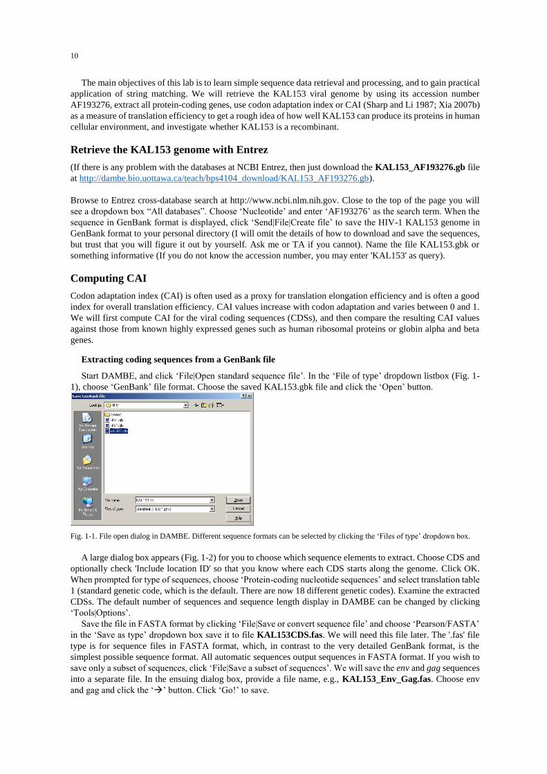
Start DAMBE, and click ‘File|Open standard sequence file’. In the ‘File of type’ dropdown listbox (Fig. 1-
1), choose ‘GenBank’ file format. Choose the saved KAL153.gbk file and click the ‘Open’ button.
Fig. 1-1. File open dialog in DAMBE. Different sequence formats can be selected by clicking the ‘Files of type’ dropdown box.
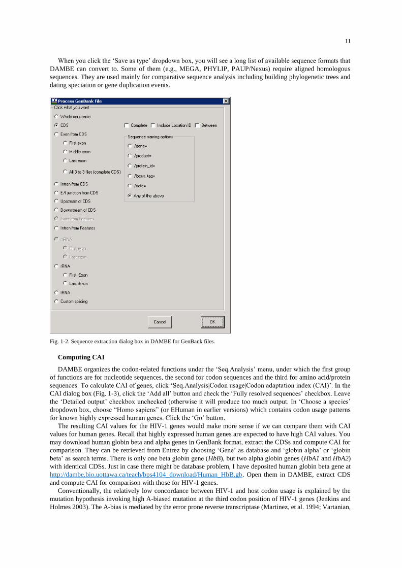
A large dialog box appears (Fig. 1-2) for you to choose which sequence elements to extract. Choose CDS and
optionally check 'Include location ID' so that you know where each CDS starts along the genome. Click OK.
When prompted for type of sequences, choose ‘Protein-coding nucleotide sequences’ and select translation table
1 (standard genetic code, which is the default. There are now 18 different genetic codes). Examine the extracted
CDSs. The default number of sequences and sequence length display in DAMBE can be changed by clicking
‘Tools|Options’.
Save the file in FASTA format by clicking ‘File|Save or convert sequence file’ and choose ‘Pearson/FASTA’
in the ‘Save as type’ dropdown box save it to file KAL153CDS.fas. We will need this file later. The '.fas' file
type is for sequence files in FASTA format, which, in contrast to the very detailed GenBank format, is the
simplest possible sequence format. All automatic sequences output sequences in FASTA format. If you wish to
save only a subset of sequences, click ‘File|Save a subset of sequences’. We will save the env and gag sequences
into a separate file. In the ensuing dialog box, provide a file name, e.g., KAL153_Env_Gag.fas. Choose env
and gag and click the ‘’ button. Click ‘Go!’ to save.
11
When you click the ‘Save as type’ dropdown box, you will see a long list of available sequence formats that
DAMBE can convert to. Some of them (e.g., MEGA, PHYLIP, PAUP/Nexus) require aligned homologous
sequences. They are used mainly for comparative sequence analysis including building phylogenetic trees and
dating speciation or gene duplication events.
Fig. 1-2. Sequence extraction dialog box in DAMBE for GenBank files.
Computing CAI
DAMBE organizes the codon-related functions under the ‘Seq.Analysis’ menu, under which the first group
of functions are for nucleotide sequences, the second for codon sequences and the third for amino acid/protein
sequences. To calculate CAI of genes, click ‘Seq.Analysis|Codon usage|Codon adaptation index (CAI)’. In the
CAI dialog box (Fig. 1-3), click the ‘Add all’ button and check the ‘Fully resolved sequences’ checkbox. Leave
the ‘Detailed output’ checkbox unchecked (otherwise it will produce too much output. In ‘Choose a species’
dropdown box, choose “Homo sapiens” (or EHuman in earlier versions) which contains codon usage patterns
for known highly expressed human genes. Click the ‘Go’ button.
The resulting CAI values for the HIV-1 genes would make more sense if we can compare them with CAI
values for human genes. Recall that highly expressed human genes are expected to have high CAI values. You
may download human globin beta and alpha genes in GenBank format, extract the CDSs and compute CAI for
comparison. They can be retrieved from Entrez by choosing ‘Gene’ as database and ‘globin alpha’ or ‘globin
beta’ as search terms. There is only one beta globin gene (HbB), but two alpha globin genes (HbA1 and HbA2)
with identical CDSs. Just in case there might be database problem, I have deposited human globin beta gene at
http://dambe.bio.uottawa.ca/teach/bps4104_download/Human_HbB.gb. Open them in DAMBE, extract CDS
and compute CAI for comparison with those for HIV-1 genes.
Conventionally, the relatively low concordance between HIV-1 and host codon usage is explained by the
mutation hypothesis invoking high A-biased mutation at the third codon position of HIV-1 genes (Jenkins and
Holmes 2003). The A-bias is mediated by the error prone reverse transcriptase (Martinez, et al. 1994; Vartanian,

12
et al. 2002) and the human APOBEC3 protein (Yu, et al. 2004). The frequency of A can reach up to 40% in
some HIV-1 genomes (Vartanian, et al. 2002), resulting in a preponderance of A-ending codons which are
typically rarely used in the host genes (Sharp 1986; Kypr and Mrazek 1987). However, a recent study suggests
that the host tRNA pool changes substantially between early and late stage of HIV-1 gene expression (van
Weringh, et al. 2011), with HIV-1 early genes adapting to the normal T-cell tRNA pool and having codon usage
similar to human genes and HIV-1 late genes adapting to the late tRNA pool. Anna van Weringh was a BPS4104
student who took the lead in this study as an MSc student in my lab.
Fig. 1-3. Dialog box for computing the codon adaptation index (CAI) in DAMBE.
Which subtype does KAL153 belong to? Is it recombinant?
Subtypes in HIV-1 M group
There are nine subtypes labelled as A, B, C, D, F, G, H, J, and K in the M group of HIV-1. Their genomic
sequences can be retrieved from either GenBank hosted at NCBI, HIV Databases hosted by Las Alamos National
Laboratory at http://www.hiv.lanl.gov/, or my University of Ottawa download page for teaching at
http://dambe.bio.uottawa.ca/teach/bps4104_download/download.aspx. It is important to know which subtype in
the HIV-1 M group (where M stands for “major”) your HIV-1 strain belongs to because different subtypes may
have different viral properties and respond to AIDS drugs differently. Identification of subtypes are typically
done by sequencing the env and gag genes and then following one of two approaches. The first is simply to
BLAST your gag and env sequences against the reference set of subtype sequences. If your query sequence
matched subtype A sequence much better than all other subtypes, then your query belong to subtype A. The
second is to construct a phylogenetic tree with all subtypes and the new HIV-1 sequence and see which subtype
clusters together with your new HIV-1 sequence. If your new sequence is clustered with subtype A with high
confidence, then your HIV-1 sequence belongs to subtype A.
Retrieve reference subtype sequences
To retrieve subtype reference sequences from Las Alamos HIV Databases, browse to
http://www.hiv.lanl.gov/content/sequence/NEWALIGN/align.html, choose ‘Subtype reference’ in ‘Alignment
type’ field, ‘ENV’ or ‘GAG’ in the ‘Pre-defined region of the genome, ‘M group without recombinants (A-K)’
in the subtype field, and click the ‘Get Alignment’ bottom to retrieve the aligned sequences in FASTA format.

13
Save the retrieved sequences in files such as RefEnv.fas and RefGag.fas. These sets of reference sequences are
aligned, but have five problems. First, they were not updated since 2010. Second, they are inconsistent with the
sequence annotation in the NCBI GenBank files. Third, contains multiple inframe stop codons which should not
appear in functional coding sequences. Fourth, the alignment quality appears poor. Fifth, some sequences are
very short and may be partial sequences. For this reason, it is better to extract the env and gag sequences from
GenBank files and filter out poor and incomplete sequences. I have done this and deposited the resulting env
and gag sequences at http://dambe.bio.uottawa.ca/teach/bps4104_download/download.aspx in two files:
RefGag.fas and RefEnv.fas. Please download these two files and save in a directory, so that we can perform
subtype identification by using BLAST.
Use BLAST to identify subtypes
(All input and output files in this section need to have no space in the file name or directory name. You will
have an error if you have a file such as C:\My Documents\MyFile.fas because there is a space in ‘My
Documents’, or C:\Temp\Test File.fas because there is a space in ‘Test file.fas’.)
Create local BLAST libraries: BLAST libraries facilitate repeated searches by preprocessing the target
(database) sequences so that search results can be returned quickly in response to a user query. We will create
two BLAST libraries, one from RefEnv.fas and the other from Ref.Gag.fas.
DAMBE uses the NCBI program makeblastdb.exe to create BLAST libraries. Start DAMBE and click
‘Alignment|BLAST’. In the dialog box (Fig. 1-4), select RefEnv.fas and specify the directory where the
resulting BLAST library will be stored. Click the ‘OK’ button and the library will be created. Do the same for
RefGag.fas.
Fig. 1-4. Dialog box for creating a local BLAST library.
BLAST against a BLAST library: DAMBE uses NCBI’s blastn.exe and blastp.exe to do nucleotide and
protein BLAST searches. Click ‘Alignment|BLAST’. In the ensuing dialog box, choose BLAST in the top
dropdown box (Fig. 1-5). Use KAL153_env_gag.fas as the input FASTA file, and the previously created
BLAST library RefEnv as the ‘Local BLAST DB’. The other options are all self-explanatory as you have already
learned E-value and word size in the lecture. The ‘Ungapped BLAST’ will not allow indels and usually should

14
not be checked. The ‘Strand’ has three options: plus, minus and both. ‘minus’ means search the complementary
strand.
Fig. 1-5. Options for basic local BLAST in DAMBE.
Click ‘OK’ and you will obtain the BLAST result for the query sequence KAL153_env of which a short
version is shown in Table 1-1. The matching quality is ranked from the highest BitScore to the lowest. We see
that KAL153 env matches subtype B best. Perform the same BLAST against the RefGag library and record
which subtype is hit with the highest BitScore. You will need these information to answer one of the lab
questions.
Table 1-1. Partial output from BLAST KAL153 env sequence against env sequences of reference subtypes.
SubType QueryStart QueryEnd DB_SeqStart DB_SeqEnd E-Val BitScore
B 31 1820 43 1868 0 2342
B 23 1820 32 1865 0 2074
B 42 1820 60 1868 0 2017
B 1 22 1 22 0.002 36.2
D 25 1820 34 1856 0 1652
D 31 1820 40 1859 0 1628
F2 23 1820 53 1871 0 1600
D 25 1820 34 1844 0 1585
D 23 1820 32 1832 0 1578
A1 1 1817 1 1835 0 1555
C 91 1820 100 1832 0 1513
H 27 1803 27 1818 0 1506
A2 32 1802 33 1802 0 1474
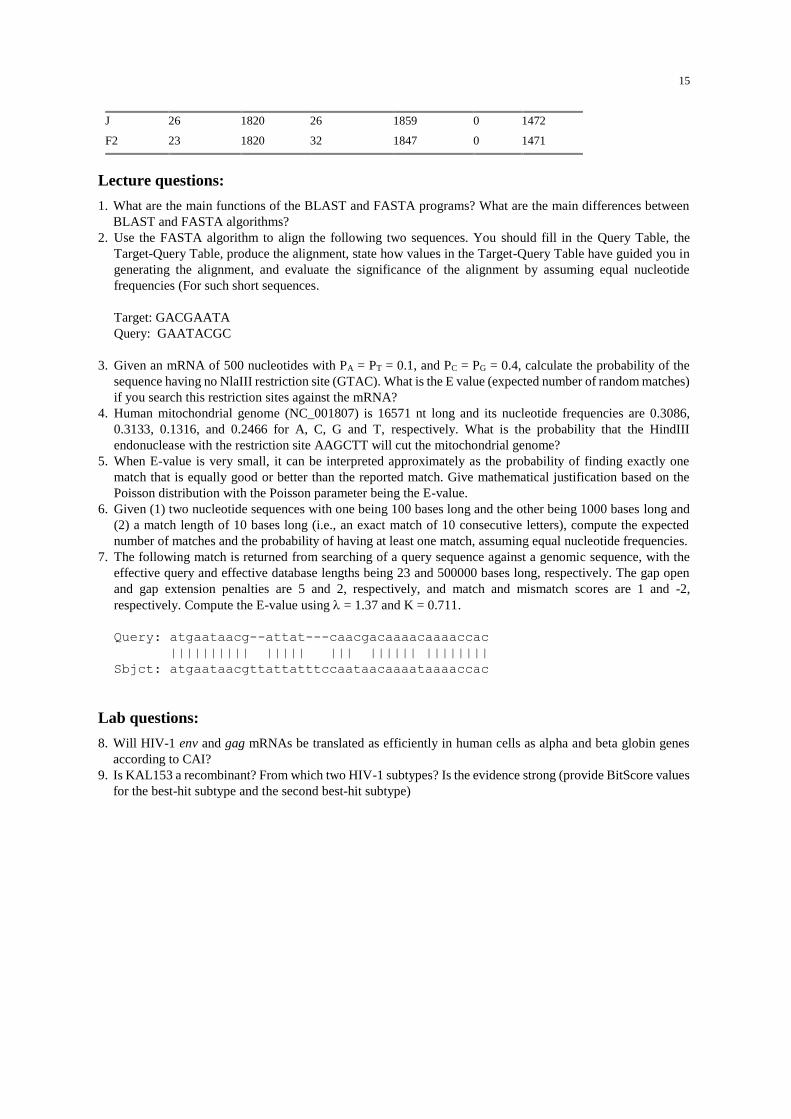
15
J 26 1820 26 1859 0 1472
F2 23 1820 32 1847 0 1471
Lecture questions:
1. What are the main functions of the BLAST and FASTA programs? What are the main differences between
BLAST and FASTA algorithms?
2. Use the FASTA algorithm to align the following two sequences. You should fill in the Query Table, the
Target-Query Table, produce the alignment, state how values in the Target-Query Table have guided you in
generating the alignment, and evaluate the significance of the alignment by assuming equal nucleotide
frequencies (For such short sequences.
Target: GACGAATA
Query: GAATACGC
3. Given an mRNA of 500 nucleotides with PA = PT = 0.1, and PC = PG = 0.4, calculate the probability of the
sequence having no NlaIII restriction site (GTAC). What is the E value (expected number of random matches)
if you search this restriction sites against the mRNA?
4. Human mitochondrial genome (NC_001807) is 16571 nt long and its nucleotide frequencies are 0.3086,
0.3133, 0.1316, and 0.2466 for A, C, G and T, respectively. What is the probability that the HindIII
endonuclease with the restriction site AAGCTT will cut the mitochondrial genome?
5. When E-value is very small, it can be interpreted approximately as the probability of finding exactly one
match that is equally good or better than the reported match. Give mathematical justification based on the
Poisson distribution with the Poisson parameter being the E-value.
6. Given (1) two nucleotide sequences with one being 100 bases long and the other being 1000 bases long and
(2) a match length of 10 bases long (i.e., an exact match of 10 consecutive letters), compute the expected
number of matches and the probability of having at least one match, assuming equal nucleotide frequencies.
7. The following match is returned from searching of a query sequence against a genomic sequence, with the
effective query and effective database lengths being 23 and 500000 bases long, respectively. The gap open
and gap extension penalties are 5 and 2, respectively, and match and mismatch scores are 1 and -2,
respectively. Compute the E-value using = 1.37 and K = 0.711.
Query: atgaataacg--attat---caacgacaaaacaaaaccac
|||||||||| ||||| ||| |||||| ||||||||
Sbjct: atgaataacgttattatttccaataacaaaataaaaccac
Lab questions:
8. Will HIV-1 env and gag mRNAs be translated as efficiently in human cells as alpha and beta globin genes
according to CAI?
9. Is KAL153 a recombinant? From which two HIV-1 subtypes? Is the evidence strong (provide BitScore values
for the best-hit subtype and the second best-hit subtype)
16
LAB 2 MAKING SENSE OF GENOMES: POSITION WEIGHT MATRIX
(PWM)
Introduction
We know that the genome is shared among all our somatic cells which nevertheless look, behave and function
quite differently. These morphological, physiological and functional diversifications are achieved mainly
through genetic switches (regulatory motifs) present in the genome that are turned on and off in different cell
types during their development. Many of these switches are present in the 5’ upstream or 3’ downstream of
individual genes (e.g., transcription and translation start and termination sites,promotor and transcription factor
binding sites, etc.). Some are also present inside genes (e.g., 5’ and 3’ splice sites and branchpoint site), and
some could be up to 1 million bases away from the gene (e.g., enhancers). To study these regulatory motifs we
need to gain the skill of manipulating genomic sequences, such as extract different sequence elements in order
to discover and characterize such motifs.
Position weight matrix (PWM) is for characterizing a set of known motifs, e.g., five nucleotides flanking the
start codon in mammalian genes. It has two purposes. The first is to know what is special about the motif for it
to be recognized by the cellular machinery, e.g., the start codon motif recognized by the translation machinery,
or the splice site motif recognized by the spliceosome. The second purpose is to use PWM to scan a sequence to
detect the presence of such motifs.
PWM also serve as a key component in De novo motif discovery algorithms such as Gibbs sampler. De novo
motif discovery refers to the process of finding a motif in a sequence but we do not know what the motif is like
and where it is located in the sequence. We will learn Gibbs sampler in a later laboratory.
Two approaches to understand the meaning of a nucleotide sequence
There are two main approaches to understand the meaning of a sequence. The first is to check against the
existing “gene dictionary”. You may not find an exact match, but a near-exact match can be helpful, in the same
way when you look for “favour” but find “favor” in the dictionary. Such checking against the “gene dictionary”
is almost exclusively done by using BLAST or FASTA suites of programs, and has become more and more
useful with the improvement of gene dictionaries (in the form of BLAST databases).
The second approach to annotate a sequence is gene prediction based on known gene features (Burge and
Karlin 1997; Salzberg, et al. 1998). For example, to scan for the presence of a protein-coding gene in a
mammalian sequence, one would first search for an open reading frame (ORF), check for the presence of 1)
Kozak consensus (RccAUGG) flanking the putative start codon, 2) 5’ and 3’ splice sites defining the exon-intron
boundary and the branchpoint site near the 3’ splice site, and 3) poly(A) signal after the stop codon. This
approach becomes essential when we find no match in the “gene dictionary” or when we find a match with no
explanation.
The effectiveness of the gene prediction approach depends on how well we know the genomic language. An
expert in English, when presented with an English sentence containing a new word, can almost instantly point
out if the new word is a noun or a verb or whether the word serves as a subject or object. In contrast, a person
knowing no English could infer little. For this reason, gene prediction algorithms typically need to be trained by
existing knowledge about genes.
Finding and specifying the meaning of a sequence is called sequence annotation. All NCBI-curated genomic
sequences represent well-annotated sequences from which we can extract coding sequences, exons, introns,
rRNAs, tRNAs and upstream and downstream sequences for detailed analysis. A more rigorous type of gene
annotation is called GO annotation, i.e., sequence annotation according to gene ontology (GO). A GO-annotated
gene contains the three minimum pieces of information: 1) the function of the gene product, 2) the biological
processes the gene product participates in, and 3) cellular localization. We will not have time to learn GO-
annotation in this course.
Extraction of annotated gene features from GenBank files
Extracting sequence elements from GenBank files is an essential skill in bioinformatics. For example, in order
to let E. coli produce a human protein, we need not only to insert the human gene into the E. coli genome, but
also to add a Shine-Dalgarno sequence to facilitate the localization of the initiation codon, to optimize its codon
usage to increase translation elongation efficiency, and to incorporate a strong promoter to facilitate
transcription. To optimize codon usage, we need to extract the tRNAs and use codons recognized by the most

17
abundant tRNAs. We can also extract the highly expressed E. coli genes to find their codon usage as a reference.
To have a good Shine-Dalgarno sequence, we again can do two things involving sequence extraction. First, we
can extract the small subunit rRNA to obtain its 3’ sequences. Second, we can extract the sequences upstream
of highly expressed E. coli genes, identify the Shine-Dalgarno sequence and obtain their consensus. One may
also be interested in knowing what is the best 5’ UTR for loading ribosomes during translation (Xia, et al. 2011)
and therefore need to extract the 5’ UTR sequences. Extraction of intron splice sites have revealed a strong
correlation between a strong splice site and protein production (Ma and Xia 2011) and advanced our
understanding of alternative splicing through exon skipping (Vlasschaert, et al. 2016). The first author of the
paper, Caitlyn Vlasschaert, is one of the former BPS4104 students, and she published two papers in her first year
as an MSc student at University of Ottawa.
Extracting sequence fragment is also necessary for making inter-specific comparisons. For example, to study
the evolution or functional changes of the coding sequences of the elongation factor EF-1, it is necessary to
splice out the CDS regions of EF-1 and join them together, and repeat this process for more than one species
in order to make inter-specific comparisons. Similarly, to study the evolution of introns of EF-1, one would
need to splice out the introns from a variety of organisms and make comparisons among them.
Position weight matrix
Extracting specific sequence components is always associated with specific analysis to address specific
biological problems. In this lab, we will extract the sequence fragments at the exon-intron junctions and use
position weight matrix (PWM) to characterize 5’ and 3’ splice sites. Such a PWM can then be used to scan
sequences for putative 5’ and 3’ splice sites to aid sequence annotation. It has also been found that 5’ and 3’
splice sites with a high PWM score (PWMS) are more efficient in recruiting spliceosome than those with a low
PWMS and that splice sites with a strongly negative PWMS are spliced by non-spliceosome mechanisms (Ma
and Xia 2011). PWM has been numerically illustrated in Xia (2007a, Chapter 5), and reviewed much more
thoroughly, with particular reference to the associated statistical significance tests in Xia (2012).
Objectives
Extracting exon-intron junctions: Specifically, we will extract the 5’ splice sites from intron-containing
genes in the yeast (Saccharomyces cerevisiae), e.g., 5 nucleotide sites on the exon side and 12 nucleotide sites
on the intron side. While we know that a spliceosome intron typically starts with GT, there are often GT
dinucleotides that do not represent the beginning of an intron. The spliceosome must have used additional
information to decide whether a particular GT represents the beginning of an intron, and this additional
information is likely in the sequences flanking the GT dinucleotide.
Characterize the sequence features of the 5’ splice site by PWM: We will learn whether there are
significant signals in nucleotides flanking the GT dinucleotide at the beginning of intron and how we can use
PWM to find similar signals in new sequences.
Procedures
A brief peek into a GenBank file
We will work with the genome of the yeast Saccharomyces cerevisiae. The GenBank file Sc.gbk file is
available at http://dambe.bio.uottawa.ca/teach/bps4104_download/download.aspx. The file (about 25 MB)
contains annotated genomic sequences for 16 chromosomes of the yeast. Right-click the Sc.gbk link, choose
‘Save target as’ and save to Sc.gbk in your personal directory. You can download the chromosome sequences
from NCBI, but it may take longer.
It is a good idea to have a look at the file which is in plain text. Click ‘File|Load text file into display’, browse
to the directory you saved the Sc.gbk, and click the ‘Open’ button. Each annotated chromosome has its own
LOCUS and ACCESSION (which may be the same or different). The ‘DEFINITION’ tells us that this LOCUS
is for the first chromosome of the yeast. PageDown to ‘FEATURES’ table and note that the first chromosome
consists 230208 nucleotides numbered from 1 to 230208. PageDown further and you will find the first annotated
coding sequences (CDS) in chromosome 1 for gene PAU8, which spans sites from 1807 to 2169 on the
complementary strand. Click ‘Edit|Find’ and input ‘join(’ to find CDSs resulting from the joining of several
exons separated by introns. The first intron-containing gene is SNC1, whose CDS results from the joining of two
exons, one spanning sites from 87287 to 87388 and the other from 87502 to 87753. The single intron naturally

18
spans the sites from 87389 to 87501. If we wish to obtain its 5’ splice site, with 5 nucleotides on the exon side
and 12 nucleotide from the intron side, then we simply extract sites spanning 87384 to 87400.
Extracting annotated sequence elements with DAMBE
Click ‘File|Open standard sequence file’. The standard Windows file open dialog appears for you to browse
to and open Sc.gbk. A dialog appears with a long list of options such as CDS, tRNA, rRNA, etc., for you to
choose what to extract from the input file. You have already learned how to extract CDSs from a GenBank file
in the first lab, but let’s practice it once more. Click ‘CDS’ and then click OK. A dialog appears with three
options: non-protein sequence, amino acid sequence, and protein-coding nucleotide sequence. Choose the last
and choose the relevant translation table out of 17 implemented genetic codes. In our case with the yeast nuclear
genome, choose 1 (the default). Click the GO button. The sequences will be displayed. Recall that we computed
CAI for HIV-1 CDSs in our last laboratory. You may practice CAI computation for the yeast genes. Save the
CDSs to file Sc_CDS.fas
To appreciate the importance of inputting the correct genetic code, click ‘Sequece|Work on amino acid
sequene’. DAMBE will translate the codon sequences into amino acid sequences. There should be no ‘*’ (which
indicates an inframe stop codon) embedded in the sequence (which is typical of functional protein-coding genes).
Click ‘Sequence|Work on codon sequences’ to restore the original codon sequences. Now choose a wrong
genetic code by clicking ‘Sequences|Change Seq.Type’ and changing the genetic code to vertebrate
mitochondrial (VertMtDNA). Now again click ‘Sequences|Work on amino acid sequences’, and you may see a
number of ‘*’ embedded in the sequence resulting from translation based on a wrong genetic code (translation
table). On the other hand, if your sequences do have an embedded stop codon UGA (common in pseudogenes),
and you choose translation table 4, then the stop codon will be mistranslated into tryptophan.
Practice with extraction of introns from CDS specifications by opening Sc.gbk and choosing ‘Intron from
CDS’. Have you noticed anything common among the introns? Spliceosome in the yeast is simpler than that in
multicellular eukaryotes and the intron splice signals are consequently stronger in the yeast than in multicellular
eukaryotes. There are only major-class introns in the yeast, and they generally start with GT dinucleotide and
end with AG dinucleotide.
Characterize 5’ and 3’ splice sites with position weight matrix (PWM)
Open the Sc.gbk file again. Note that DAMBE keeps four most recently opened files under the ‘File’ menu.
If you have opened Sc.gbk recently, just click it under the ‘File’ menu. When presented with a dialog for you to
choose which sequence feature to extract (Fig. 2-1), click ‘E/I junctions from CDS’. Extract 5 nucleotides on
the exon side and 12 nucleotides on the intron side by entering ‘5,12’ (which is in fact the default). Click ‘Non-
protein sequences’ when prompted for sequence type. Some sequences may be identical and you may be asked
if you wish to merge identical sequences. Click ‘No’.
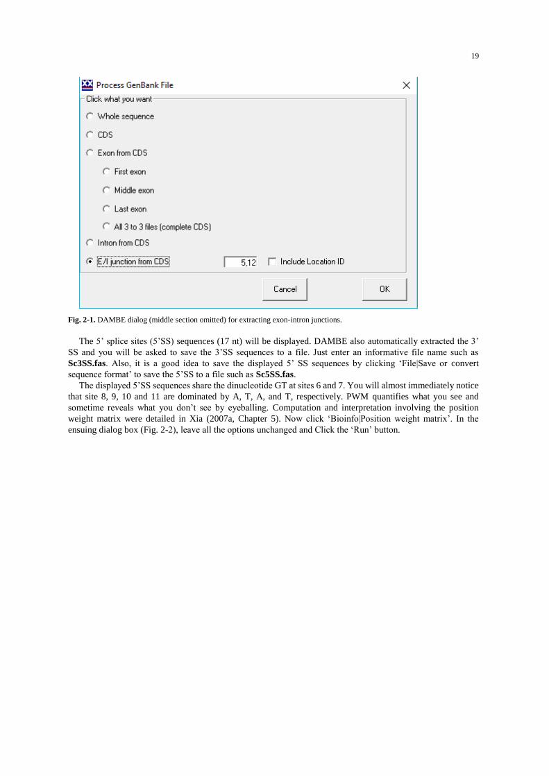
19
Fig. 2-1. DAMBE dialog (middle section omitted) for extracting exon-intron junctions.
The 5’ splice sites (5’SS) sequences (17 nt) will be displayed. DAMBE also automatically extracted the 3’
SS and you will be asked to save the 3’SS sequences to a file. Just enter an informative file name such as
Sc3SS.fas. Also, it is a good idea to save the displayed 5’ SS sequences by clicking ‘File|Save or convert
sequence format’ to save the 5’SS to a file such as Sc5SS.fas.
The displayed 5’SS sequences share the dinucleotide GT at sites 6 and 7. You will almost immediately notice
that site 8, 9, 10 and 11 are dominated by A, T, A, and T, respectively. PWM quantifies what you see and
sometime reveals what you don’t see by eyeballing. Computation and interpretation involving the position
weight matrix were detailed in Xia (2007a, Chapter 5). Now click ‘Bioinfo|Position weight matrix’. In the
ensuing dialog box (Fig. 2-2), leave all the options unchanged and Click the ‘Run’ button.
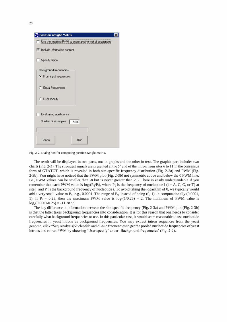
20
Fig. 2-2. Dialog box for computing position weight matrix.
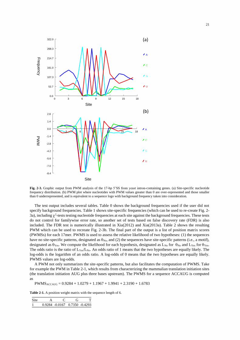
The result will be displayed in two parts, one in graphs and the other in text. The graphic part includes two
charts (Fig. 2-3). The strongest signals are presented at the 5’ end of the intron from sites 6 to 11 in the consensus
form of GTATGT, which is revealed in both site-specific frequency distribution (Fig. 2-3a) and PWM (Fig.
2-3b). You might have noticed that the PWM plot (Fig. 2-3b) not symmetric above and below the 0 PWM line,
i.e., PWM values can be smaller than -8 but is never greater than 2.3. There is easily understandable if you
remember that each PWM value is log2(Pij/Pi), where Pij is the frequency of nucleotide i (i = A, C, G, or T) at
site j, and Pi is the background frequency of nucleotide i. To avoid taking the logarithm of 0, we typically would
add a very small value to Pij, e.g., 0.0001. The range of Pij, instead of being (0, 1), in computationally (0.0001,
1). If Pi = 0.25, then the maximum PWM value is log2(1/0.25) = 2. The minimum of PWM value is
log2(0.0001/0.25) = -11.2877.
The key difference in information between the site-specific frequency (Fig. 2-3a) and PWM plot (Fig. 2-3b)
is that the latter takes background frequencies into consideration. It is for this reason that one needs to consider
carefully what background frequencies to use. In this particular case, it would seem reasonable to use nucleotide
frequencies in yeast introns as background frequencies. You may extract intron sequences from the yeast
genome, click “Seq.Analysis|Nucleotide and di-nuc frequencies to get the pooled nucleotide frequencies of yeast
introns and re-run PWM by choosing ‘User specify’ under ‘Background frequencies’ (Fig. 2-2).
21
A
C
G
U
Fre
quency
Site
0.0
53.7
107.3
161.0
214.7
268.3
322.0
0 3 6 9 12 15 18
A
C
G
U
PW
M
Site
-1.4
-2.8
-4.2
-5.6
-7.0
-8.4
0.0
1.4
2.8
3 6 9 12 15 18
(a)
(b)
Fig. 2-3. Graphic output from PWM analysis of the 17-bp 5’SS from yeast intron-containing genes. (a) Site-specific nucleotide
frequency distribution. (b) PWM plot where nucleotides with PWM values greater than 0 are over-represented and those smaller
than 0 underrepresented, and is equivalent to a sequence logo with background frequency taken into consideration.
The test output includes several tables. Table 0 shows the background frequencies used if the user did not
specify background frequencies. Table 1 shows site-specific frequencies (which can be used to re-create Fig. 2-
3a), including 2-tests testing nucleotide frequencies at each site against the background frequencies. These tests
do not control for familywise error rate, so another set of tests based on false discovery rate (FDR) is also
included. The FDR test is numerically illustrated in Xia(2012) and Xia(2013a). Table 2 shows the resulting
PWM which can be used to recreate Fig. 2-3b. The final part of the output is a list of position matrix scores
(PWMSs) for each 17mer. PWMS is used to assess the relative likelihood of two hypotheses: (1) the sequences
have no site-specific patterns, designated as No, and (2) the sequences have site-specific patterns (i.e., a motif),
designated as Yes. We compute the likelihood for each hypothesis, designated as LNo for No and LYes for Yes.
The odds ratio is the ratio of LYes/LNo. An odds ratio of 1 means that the two hypotheses are equally likely. The
log-odds is the logarithm of an odds ratio. A log-odds of 0 means that the two hypotheses are equally likely.
PWMS values are log-odds.
A PWM not only summarizes the site-specific patterns, but also facilitates the computation of PWMS. Take
for example the PWM in Table 2-1, which results from characterizing the mammalian translation initiation sites
(the translation initiation AUG plus three bases upstream). The PWMS for a sequence ACCAUG is computed
as
PWMSACCAUG = 0.9284 + 1.0279 + 1.1967 + 1.9941 + 2.3190 + 1.6783
Table 2-1. A position weight matrix with the sequence length of 6.
Site A C G T
1 0.9284 -0.0167 0.7350 -0.4293
22
2 0.4731 1.0279 -0.0072 0.1086
3 -0.0761 1.1967 0.3856 -0.3954
4 1.9941 -0.7772 -0.8254 -0.9879
5 -0.8980 -0.8743 -0.8254 2.3190
6 -0.8980 -0.8743 1.6783 -0.9879
A 5’SS with a high PWMS value indicates a strong signal. Almost all introns in highly expressed yeast genes
have high PWMS values because there is selection pressure for these genes to be spliced efficiently. A 5’SS
with no selection would be subject to mutation and would have site-specific frequencies similar to those of the
background frequencies, and the expected PWMS values for such genes is close to 0. What is puzzling is that
some 5’SS have PWMS that are strongly negative, which means that such introns are under selection pressure
to have their 5’SS not recognized by spliceosomes. Some of these genes are known to be spliced by mechanisms
other than spliceosome (Ma and Xia 2011).
Now perform the same PWM analysis for the 3’SS that you have saved in file Sc3SS.fas.
Scan sequences for splice site signals
A PWM derived from a good set of motif sequence can be used to scan for motif signals in new sequences.
For example, we can use the PWM in Table 2-1 to scan sequences with a sliding window of 6 bases, e.g., from
site 1 to site 6, from site 2 to site 7, and so on. The resulting window-specific PWMS can be used to judge
whether the 6-mer is a putative translation initiation site. Similarly, we can use our PWM derived from 5’SS or
3’SS to scan for the presence of splicing signals. One interesting finding by experimental biologists is that most
spliceosome proteins are recruited to yeast mRNAs with no introns, and one may hypothesize that those
intron-less mRNAs may happen to contain false 5’SS signals. You may use your PWM to scan yeast intron-less
genes to see which 17mer may have a high PWMS, and you would predict that those 17mers with high PWMS
values are where the spliceosome proteins are recruited.
The option to use the resulting PWM to scan another set of sequences is available at the top of the PWM
dialog box in Fig. 2-2. Click ‘Bioinformatics|Position weight matrix’ and check ‘Use the resulting PWM to scan
another set of sequences’. Click ‘Run’. You will be asked for the file name containing the sequences that you
wish to scan. Choose the saved Sc_CDS.fas. You will have the same output as before but with an additional
table showing the 17mer with the highest PWMS in each CDS. While a high PWMS in a true splice sites
represent a true splice signal, a high PWMS in an intronless gene implies a false signal. Unfortunately, the
spliceosome proteins are attracted to splice signals, whether they are false or true. These PWMS values can be
used to test our hypothesis that many spliceosome proteins are recruited by intron-less yeast mRNAs with strong
but false splice site signals.
Limitations of PWM
PWM cannot detect site dependence. For example, if nucleotides at two positions form base pairs, then the
information is contained in the two positions jointly but not individually. The two sites can classify the eight
sequences below into four groups, but a conventional PWM will conclude that the two sites are not informative.
…A…T…
…A…T…
…C…G…
…C…G…
…G…C…
…G…C…
…T…A…
…T…A…
One way to extend PWM to site dependence is to recode sites as doublets. For example, if site-dependence
occurs only between neighboring sites, then we can modify PWM to detect the neighboring site dependence, by
using the 16 dinucleotides instead of the four nucleotides. For example, a 6-mer CCCGGG contains five
dinucleotides, i.e., CC, CC, CG, GG, GG. An further extension of this is that we may take a nucleotide at position
i and another nucleotide at position i+k as a dinucleotide.
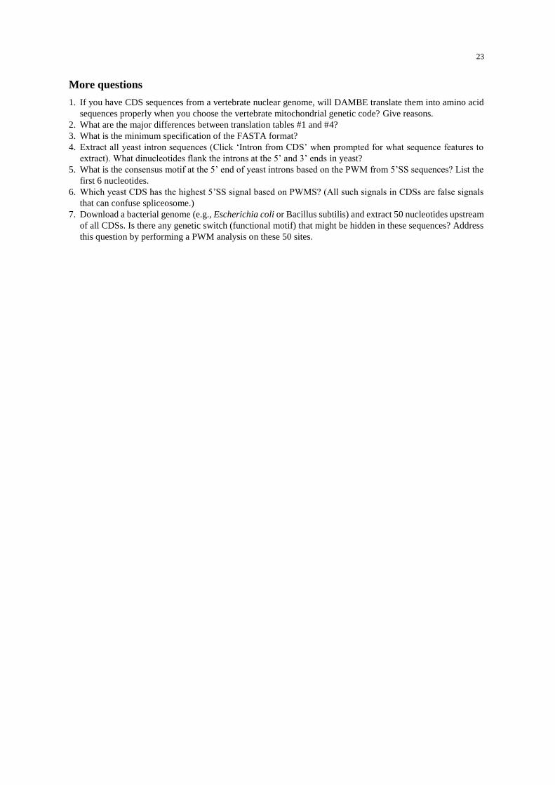
23
More questions
1. If you have CDS sequences from a vertebrate nuclear genome, will DAMBE translate them into amino acid
sequences properly when you choose the vertebrate mitochondrial genetic code? Give reasons.
2. What are the major differences between translation tables #1 and #4?
3. What is the minimum specification of the FASTA format?
4. Extract all yeast intron sequences (Click ‘Intron from CDS’ when prompted for what sequence features to
extract). What dinucleotides flank the introns at the 5’ and 3’ ends in yeast?
5. What is the consensus motif at the 5’ end of yeast introns based on the PWM from 5’SS sequences? List the
first 6 nucleotides.
6. Which yeast CDS has the highest 5’SS signal based on PWMS? (All such signals in CDSs are false signals
that can confuse spliceosome.)
7. Download a bacterial genome (e.g., Escherichia coli or Bacillus subtilis) and extract 50 nucleotides upstream
of all CDSs. Is there any genetic switch (functional motif) that might be hidden in these sequences? Address
this question by performing a PWM analysis on these 50 sites.

24
LAB 3 GIBBS SAMPLER AND YEAST INTRON PROPERTIES
Introduction
Genetic switches
A genome with its encoded genes come to life only when the genes are activated or inactivated over time in
response to the changing cellular environment leading to the production of different proteins and RNAs at the
right time in the right location. How can a genome respond to the changing cellular environment? It can do so
because it features many genetic switches that can be flipped on or off by cellular machineries. Even simple
genomes such as that of the phage have such genetic switches (Ptashne 1986).
Genetic switches are specific sequence motifs in nature. These include transcription and translation initiation
and termination sites, transcription factor binding sites, intron-splicing sites, intron branching-point site, poly-A
site, etc., as well as a set of very important but yet poorly defined set of signals for epigenetic modification of
DNA. Finding these genetic switches in a genome not only increase our understanding of how genomes work,
but also have practical applications because many genetic switches are drug-targets.
Some sequence motifs can be experimentally characterized. Such characterized motifs can then be used to
construct a position weight matrix to scan other sequences for the presence of such motifs. However, often we
will just have a set of sequences and have no idea what the motif would look like and where it might be in the
sequence. We only have a vague idea that some genetic switch is located somewhere in all or most of these
sequences, but we do not know what and where. Gibbs sampler is one of the Monte Carlo algorithms for finding
such motifs.
Gibbs sampler and its application in molecular biology
Monte Carlo method was envisioned by the famous mathematician Stanislaw Ulam, following the successful
assembly of the first electronic computer ENIAC in 1945, and further developed by physicists and
mathematicians working on nuclear weapon projects in the Los Alamos National Laboratory in mid-1940s
(Metropolis 1987). The term “Monte Carlo method” was coined by Nicholas Metropolis to designate this class
of computational algorithms. While the development and application of the method unsurprisingly followed the
operation of ENIAC in 1945, the physicist Enrico Fermi is known to have independently developed and applied
the method nearly 15 years earlier with mechanical calculators (Metropolis 1987).
Gibbs sampler simplifies computation in parameter estimation when analytical solution is very difficult or
impossible to obtain. In biology, it has been used in the identification of functional motifs in proteins (Neuwald,
et al. 1995; Mannella, et al. 1996; Qu, et al. 1998), biological image processing (Samso, et al. 2002), pairwise
sequence alignment (Zhu, et al. 1998) and multiple sequence alignment (Holmes and Bruno 2001; Jensen and
Hein 2005). However, the most frequent biological application of Gibbs sampler in bioinformatics remains in
the identification of regulatory sequences of genes (Lawrence, et al. 1993; Thijs, et al. 2001; Thijs, Marchal, et
al. 2002; Thijs, Moreau, et al. 2002; Coessens, et al. 2003; Qin, et al. 2003; Thompson, et al. 2003; Thompson,
et al. 2004; Aerts, et al. 2005).
The core component of a Gibbs sampler is PWM (position weight matrix). The implementation of the Gibbs
sampler algorithm has been numerically illustrated before (Xia 2007a, Chapter 7; 2012). For relevant statistical
tests for the derived PWM, one should consult Xia (2012).
Identifying genetic motifs with Gibbs sampler
Imagine three scenarios. In the first, suppose you have performed microarray (Schena 1996; Schena 2003) or
SAGE (Velculescu, et al. 1995; Saha, et al. 2002) or RNA-Seq analysis of a yeast strain over time, and identified
a set of protein-coding genes that increase and decrease gene expression synchronously. Are these co-expressed
genes co-regulated? They may be co-regulated if they share regulatory sequences in their 5'-UTR. But how
would we know if they share regulatory sequences in the 5'-UTR? With the bioinformatic skills you have gained,
you could extract, say, 2000 nt upstream of the initiation AUG that may well contain the regulatory sequence.
However, the regulatory sequences could be just a few bases long and may be anywhere in the 2000-nt sequence.
What are these regulatory sequences? Where are they located? If there are indeed shared sequence motifs hidden
somewhere in these 2000-mers, then they most likely will be found by Gibbs sampler and displayed with
information on their exact locations.
In the second scenario, imagine that you have done a control/treatment experiment on two groups of goldfish
in which the treatment is exposure to estrogen. You identified a set of genes that are upregulated. You wish to
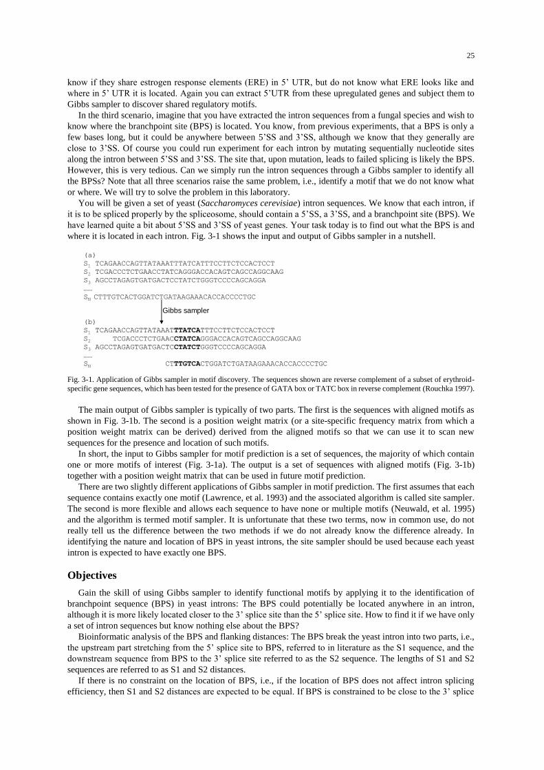
25
know if they share estrogen response elements (ERE) in 5’ UTR, but do not know what ERE looks like and
where in 5’ UTR it is located. Again you can extract 5’UTR from these upregulated genes and subject them to
Gibbs sampler to discover shared regulatory motifs.
In the third scenario, imagine that you have extracted the intron sequences from a fungal species and wish to
know where the branchpoint site (BPS) is located. You know, from previous experiments, that a BPS is only a
few bases long, but it could be anywhere between 5’SS and 3’SS, although we know that they generally are
close to 3’SS. Of course you could run experiment for each intron by mutating sequentially nucleotide sites
along the intron between 5’SS and 3’SS. The site that, upon mutation, leads to failed splicing is likely the BPS.
However, this is very tedious. Can we simply run the intron sequences through a Gibbs sampler to identify all
the BPSs? Note that all three scenarios raise the same problem, i.e., identify a motif that we do not know what
or where. We will try to solve the problem in this laboratory.
You will be given a set of yeast (Saccharomyces cerevisiae) intron sequences. We know that each intron, if
it is to be spliced properly by the spliceosome, should contain a 5’SS, a 3’SS, and a branchpoint site (BPS). We
have learned quite a bit about 5’SS and 3’SS of yeast genes. Your task today is to find out what the BPS is and
where it is located in each intron. Fig. 3-1 shows the input and output of Gibbs sampler in a nutshell.
(a)
S1 TCAGAACCAGTTATAAATTTATCATTTCCTTCTCCACTCCT
S2 TCGACCCTCTGAACCTATCAGGGACCACAGTCAGCCAGGCAAG
S3 AGCCTAGAGTGATGACTCCTATCTGGGTCCCCAGCAGGA
……
SN CTTTGTCACTGGATCTGATAAGAAACACCACCCCTGC
(b)
S1 TCAGAACCAGTTATAAATTTATCATTTCCTTCTCCACTCCT
S2 TCGACCCTCTGAACCTATCAGGGACCACAGTCAGCCAGGCAAG
S3 AGCCTAGAGTGATGACTCCTATCTGGGTCCCCAGCAGGA
……
SN CTTTGTCACTGGATCTGATAAGAAACACCACCCCTGC
Gibbs sampler
Fig. 3-1. Application of Gibbs sampler in motif discovery. The sequences shown are reverse complement of a subset of erythroid-
specific gene sequences, which has been tested for the presence of GATA box or TATC box in reverse complement (Rouchka 1997).
The main output of Gibbs sampler is typically of two parts. The first is the sequences with aligned motifs as
shown in Fig. 3-1b. The second is a position weight matrix (or a site-specific frequency matrix from which a
position weight matrix can be derived) derived from the aligned motifs so that we can use it to scan new
sequences for the presence and location of such motifs.
In short, the input to Gibbs sampler for motif prediction is a set of sequences, the majority of which contain
one or more motifs of interest (Fig. 3-1a). The output is a set of sequences with aligned motifs (Fig. 3-1b)
together with a position weight matrix that can be used in future motif prediction.
There are two slightly different applications of Gibbs sampler in motif prediction. The first assumes that each
sequence contains exactly one motif (Lawrence, et al. 1993) and the associated algorithm is called site sampler.
The second is more flexible and allows each sequence to have none or multiple motifs (Neuwald, et al. 1995)
and the algorithm is termed motif sampler. It is unfortunate that these two terms, now in common use, do not
really tell us the difference between the two methods if we do not already know the difference already. In
identifying the nature and location of BPS in yeast introns, the site sampler should be used because each yeast
intron is expected to have exactly one BPS.
Objectives
Gain the skill of using Gibbs sampler to identify functional motifs by applying it to the identification of
branchpoint sequence (BPS) in yeast introns: The BPS could potentially be located anywhere in an intron,
although it is more likely located closer to the 3’ splice site than the 5’ splice site. How to find it if we have only
a set of intron sequences but know nothing else about the BPS?
Bioinformatic analysis of the BPS and flanking distances: The BPS break the yeast intron into two parts, i.e.,
the upstream part stretching from the 5’ splice site to BPS, referred to in literature as the S1 sequence, and the
downstream sequence from BPS to the 3’ splice site referred to as the S2 sequence. The lengths of S1 and S2
sequences are referred to as S1 and S2 distances.
If there is no constraint on the location of BPS, i.e., if the location of BPS does not affect intron splicing
efficiency, then S1 and S2 distances are expected to be equal. If BPS is constrained to be close to the 3’ splice
26
site, then the S2 distance is expected to (1) be smaller than the S1 distance and (2) vary less than the expectation
based on random placement of BPS along the intron sequences. Similarly, if BPS is constrained to be close to
the 5’ splice site, then the S1 distance would expected to (1) be smaller than the S2 distance, and (2) vary less
than the expectation based on random placement of BPS along the intron sequences.
Procedures
Start DAMBE and read in the YeastAllIntron.FAS file in DAMBE’s installation directory (it is one of the sample
files that come with DAMBE). The file contains all documented yeast introns located within the coding
sequences.
We will first practice how to copy column-based output from DAMBE to EXCEL. This is needed for
subsequent data analysis on S1 and S2 distances. We will then use Gibbs sampler implemented in DAMBE to
find what the BPS is and where it is located in each intron. Once BPS is identified, S1 and S2 are defined and
can be further studied.
Copy column-based output from DAMBE to EXCEL
When the yeast intron sequences are displayed on the screen, what we see is equivalent to a two-column output,
i.e., the first column being sequence names and the second column being sequences. We will copy these two
columns into an EXCEL sheet.
Highlight all sequences, but not the numbering (Fig. 3-2), and click ‘Edit|Copy to EXCEL’. Now the sequence
name and the sequences are all copied into Windows clipboard ready to be copied into any Windows programs.
Fig. 3-2. Highlight column-based output in DAMBE for copying and pasting into EXCEL.
Launch EXCEL and label one EXCEL sheet as S1S2 (i.e., double-click the tag ‘Sheet 1’ and change it to
‘S1S2’). We will generate and store all relevant S1 and S2 distances in this sheet. In the first cell of the first
column (i.e., the A1 cell), enter ‘SeqName’ (without the single quotes) for sequence name. In the first cell of the
second column (i.e., the B1 cell), enter ‘Sequence’. Now click the second cell of the first column (i.e., the A2
cell) and click, in EXCEL, ‘Edit|Paste’. The sequence name and the sequences in the clipboard will be pasted
into EXCEL in two columns.
Now in the C1 cell, enter ‘SeqLen’ as we want this column to contain intron length. In the C2 cell, enter
‘=LEN(B2)’ and press the ‘Enter’ key in your keyboard (Fig. 3-3). The cell will display the number 113 which
means that the intron sequence in the B2 cell is 113 nucleotides long. Now move the mouse over the B2 cell to
its lower right corner so that the fat empty cross becomes a thin solid cross. Hold down the left mouse button
and drag down all the way to the last intron. The ‘C’ column will now contain the length of all introns.
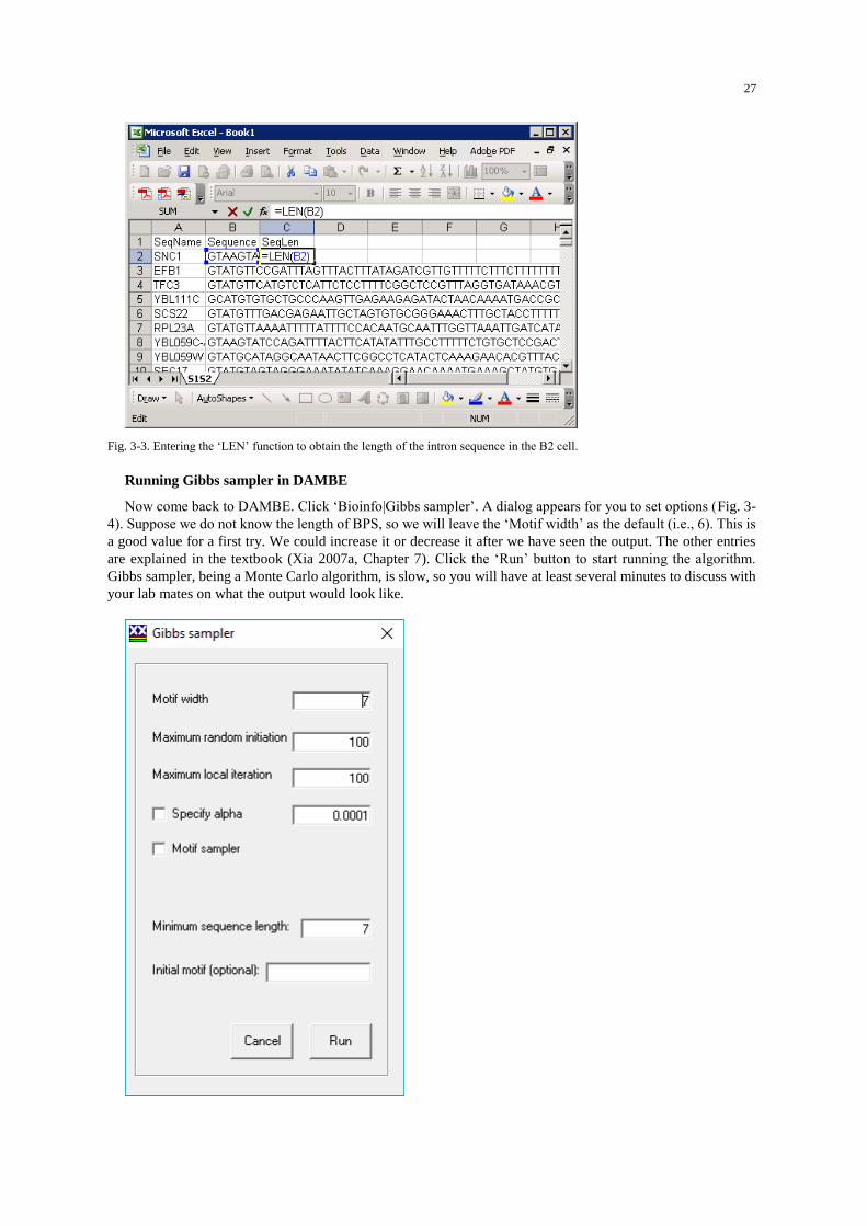
27
Fig. 3-3. Entering the ‘LEN’ function to obtain the length of the intron sequence in the B2 cell.
Running Gibbs sampler in DAMBE
Now come back to DAMBE. Click ‘Bioinfo|Gibbs sampler’. A dialog appears for you to set options (Fig. 3-
4). Suppose we do not know the length of BPS, so we will leave the ‘Motif width’ as the default (i.e., 6). This is
a good value for a first try. We could increase it or decrease it after we have seen the output. The other entries
are explained in the textbook (Xia 2007a, Chapter 7). Click the ‘Run’ button to start running the algorithm.
Gibbs sampler, being a Monte Carlo algorithm, is slow, so you will have at least several minutes to discuss with
your lab mates on what the output would look like.

28
Fig. 3-4. Setting options for Gibbs sampler in DAMBE.
Once DAMBE has finished running Gibbs sampler, the output will be presented in four parts. The first part
shows the global nucleotide frequencies. The second part shows the site-specific nucleotide frequencies for the
motifs found (Fig. 3-5). We notice that the Gibbs sampler converged after only 24 iterations. If it fails to
converge, then we have to increase the number of iterations (Fig. 3-4).
Gibbs sampler reached convergence after 24 iterations.
Final site-specific counts:
A C G U
1 275 0 4 0
2 0 272 0 7
3 0 0 1 278
4 275 1 3 0
5 278 0 1 0
6 0 276 0 3
Final site-specific frequencies:
A C G U
1 0.98330 0.00059 0.01491 0.00121
2 0.00116 0.97201 0.00062 0.02621
3 0.00116 0.00059 0.00419 0.99407
4 0.98330 0.00416 0.01133 0.00121
5 0.99401 0.00059 0.00419 0.00121
6 0.00116 0.98630 0.00062 0.01192
Fig. 3-5. Partial output from Gibbs sampler after running it on yeast intron sequences.
The partial output (Fig. 3-5) shows that the 6-mer motif is ACUAAU. The site-specific frequencies can be
used to derive a position weight matrix to rapidly scan other sequences for the presence of such motifs.
The third part of the output shows the motifs in aligned format (Fig. 3-6), with the two down arrows indicating
the start and end of the motif which is ACUAAC in most intron sequences. We also note that the nucleotide just
upstream of ACUAAC is U in most cases, so yeast BPS might be UACUAAC, i.e., a 7-mer instead of a 6-mer.
You may re-run Gibbs sampler by changing the ‘Motif width’ from the default 6 to 7.
Fig. 3-6. Partial output from running Gibbs sampler on yeast intron sequences, with the shared motifs shown in aligned format. Note
that you may need to drag the horizontal bar to the far right in order to see the aligned motifs shown.
The fourth part of the output (Table 3-1) shows the motifs found, where they start in the intron sequence and
the position weight matrix scores (PWMSs). Note that a position weight matrix score may be presented in two
ways. Sometimes it is presented as a likelihood ratio (i.e., the likelihood that there is a site-specific pattern,
designated as LYes, and the likelihood that there is no site-specific pattern, designated as LNo), but sometimes it
is presented as the base-2 logarithm of the likelihood ratio. The two likelihood values for the motif ACUAAC
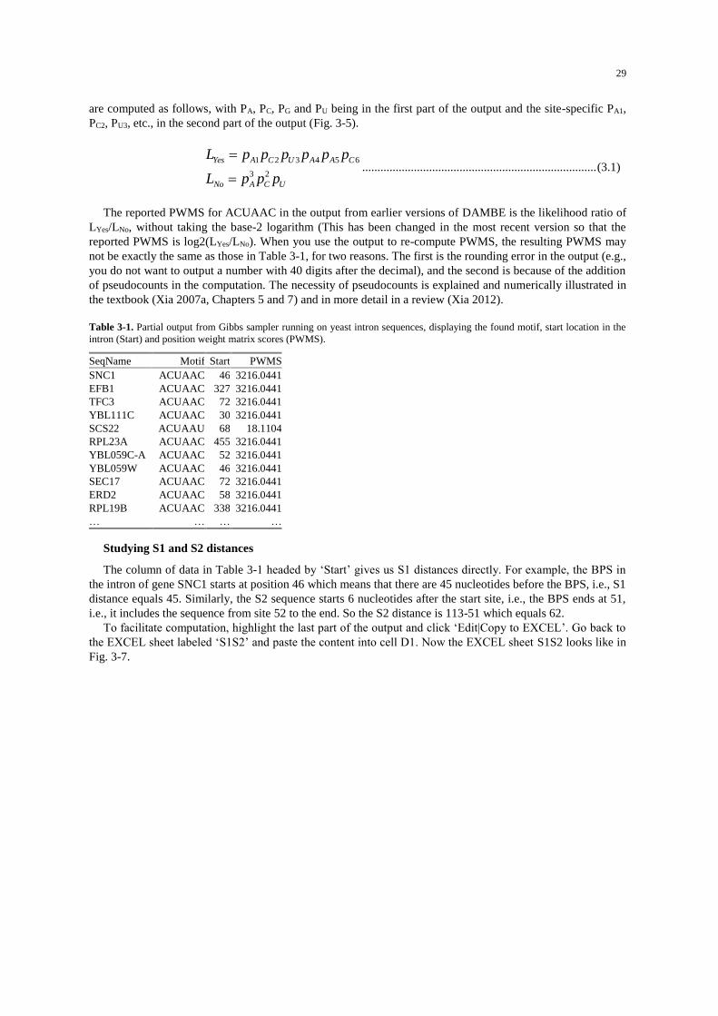
29
are computed as follows, with PA, PC, PG and PU being in the first part of the output and the site-specific PA1,
PC2, PU3, etc., in the second part of the output (Fig. 3-5).
1 2 3 4 5 6
3 2
Yes A C U A A C
No A C U
L p p p p p p
L p p p
............................................................................. (3.1)
The reported PWMS for ACUAAC in the output from earlier versions of DAMBE is the likelihood ratio of
LYes/LNo, without taking the base-2 logarithm (This has been changed in the most recent version so that the
reported PWMS is log2(LYes/LNo). When you use the output to re-compute PWMS, the resulting PWMS may
not be exactly the same as those in Table 3-1, for two reasons. The first is the rounding error in the output (e.g.,
you do not want to output a number with 40 digits after the decimal), and the second is because of the addition
of pseudocounts in the computation. The necessity of pseudocounts is explained and numerically illustrated in
the textbook (Xia 2007a, Chapters 5 and 7) and in more detail in a review (Xia 2012).
Table 3-1. Partial output from Gibbs sampler running on yeast intron sequences, displaying the found motif, start location in the
intron (Start) and position weight matrix scores (PWMS).
SeqName Motif Start PWMS
SNC1 ACUAAC 46 3216.0441
EFB1 ACUAAC 327 3216.0441
TFC3 ACUAAC 72 3216.0441
YBL111C ACUAAC 30 3216.0441
SCS22 ACUAAU 68 18.1104
RPL23A ACUAAC 455 3216.0441
YBL059C-A ACUAAC 52 3216.0441
YBL059W ACUAAC 46 3216.0441
SEC17 ACUAAC 72 3216.0441
ERD2 ACUAAC 58 3216.0441
RPL19B ACUAAC 338 3216.0441
… … … …
Studying S1 and S2 distances
The column of data in Table 3-1 headed by ‘Start’ gives us S1 distances directly. For example, the BPS in
the intron of gene SNC1 starts at position 46 which means that there are 45 nucleotides before the BPS, i.e., S1
distance equals 45. Similarly, the S2 sequence starts 6 nucleotides after the start site, i.e., the BPS ends at 51,
i.e., it includes the sequence from site 52 to the end. So the S2 distance is 113-51 which equals 62.
To facilitate computation, highlight the last part of the output and click ‘Edit|Copy to EXCEL’. Go back to
the EXCEL sheet labeled ‘S1S2’ and paste the content into cell D1. Now the EXCEL sheet S1S2 looks like in
Fig. 3-7.
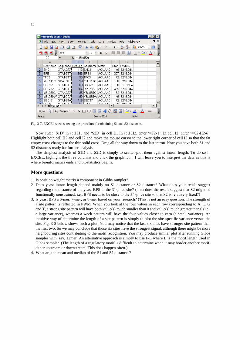
30
Fig. 3-7. EXCEL sheet showing the procedure for obtaining S1 and S2 distances.
Now enter ‘S1D’ in cell H1 and ‘S2D’ in cell I1. In cell H2, enter ‘=F2-1’. In cell I2, enter ‘=C2-H2-6’.
Highlight both cell H2 and cell I2 and move the mouse cursor to the lower right corner of cell I2 so that the fat
empty cross changes to the thin solid cross. Drag all the way down to the last intron. Now you have both S1 and
S2 distances ready for further analysis.
The simplest analysis of S1D and S2D is simply to scatter-plot them against intron length. To do so in
EXCEL, highlight the three columns and click the graph icon. I will leave you to interpret the data as this is
where bioinformatics ends and biostatistics begins.
More questions
1. Is position weight matrix a component in Gibbs sampler?
2. Does yeast intron length depend mainly on S1 distance or S2 distance? What does your result suggest
regarding the distance of the yeast BPS to the 3' splice site? (hint: does the result suggest that S2 might be
functionally constrained, i.e., BPS needs to be close to the 3’ splice site so that S2 is relatively fixed?)
3. Is yeast BPS a 6-mer, 7-mer, or 8-mer based on your research? (This is not an easy question. The strength of
a site pattern is reflected in PWM. When you look at the four values in each row corresponding to A, C, G
and T, a strong site pattern will have both value(s) much smaller than 0 and value(s) much greater than 0 (i.e.,
a large variance), whereas a week pattern will have the four values closer to zero (a small variance). An
intuitive way of determine the length of a site pattern is simply to plot the site-specific variance versus the
site. Fig. 3-8 below shows such a plot. You may notice that the last six sites have stronger site pattern than
the first two. So we may conclude that those six sites have the strongest signal, although there might be more
neighbouring sites contributing to the motif recognition. You may produce similar plot after running Gibbs
sampler with, say, 12mer. An alternative approach is simply to use F/L where L is the motif length used in
Gibbs sampler. (The length of a regulatory motif is difficult to determine when it may border another motif,
either upstream or downstream. This does happen often.)
4. What are the mean and median of the S1 and S2 distances?
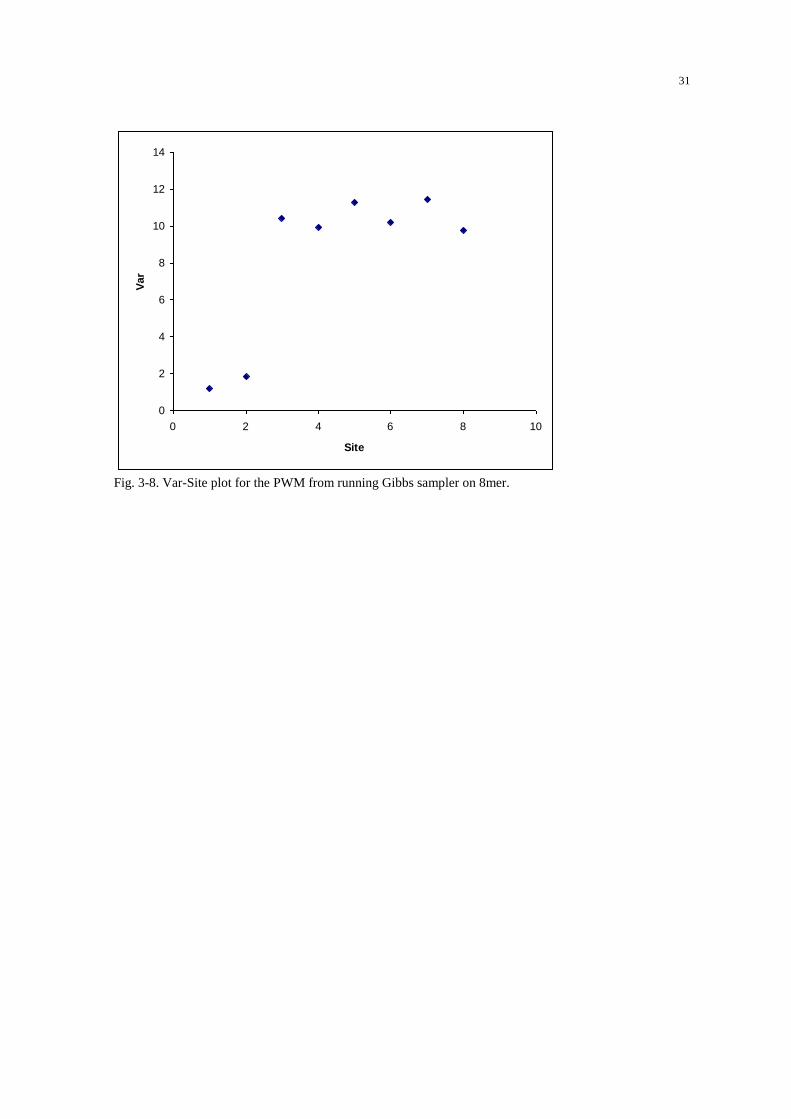
31
Fig. 3-8. Var-Site plot for the PWM from running Gibbs sampler on 8mer.
0
2
4
6
8
10
12
14
0 2 4 6 8 10
Site
Var
32
LAB 5 CODON USAGE BIAS
Introduction
Genetic codes are degenerate. For example, glycine is coded by four synonymous codons (GGN, where N
stands for any nucleotide) and lysine is coded by two synonymous codons (AAR, where R stands for either A
or G). Some synonymous codons are used much more frequently than others. Differential usage of synonymous
codons is termed codon usage bias.
This laboratory has two parts. The first part is on codon usage bias and indices frequently used to measure
the codon usage bias. These indices are often used as an indirect measure of gene expression because
experimental data have repeated demonstrated a close correlation between gene expression and codon bias
indices (Comeron and Aguade 1998; Coghlan and Wolfe 2000).
Because eukaryotic viruses and bacteriophages generally do not have their own translation machinery, they
typically evolve codon usage in response to their host tRNA pools. Several students in my laboratory have made
significant contributions along this line of enquiry, including HIV-1 codon adaptation to human T-cell tRNA
pool (van Weringh, et al. 2011), codon adaptation in E. coli phages in response to host tRNA pool and the effect
of phage-encoded tRNA on this adaptation (Chithambaram, et al. 2014a, b; Prabhakaran, et al. 2014), and how
codon adaptation in phages is mediated by other processes such as translation initiation (Prabhakaran, et al.
2015).
The second part is for identifying tRNA anticodon, which is often necessary to understand codon usage bias.
Two factors are known to affect codon usage bias. The first is the mutation bias (Muto and Osawa 1987; Xia
2005), i.e., AT-biased mutation will increase the usage of A-ending and T-ending codons. The second is the
tRNA-mediated selection to improved efficiency and accuracy in translation (Ikemura 1981a; Bulmer 1987;
Ikemura 1992; Xia 1998a; Xia, et al. 2007; Carullo and Xia 2008; Xia 2008). Different synonymous codons in
a codon family are often translated by different tRNA species (isoaccepting tRNAs) which exist in different
concentrations in the cell. It is understandable that, if many tRNAs are available to translate glycine codons
GGC and GGU but few tRNAs are available to translate glycine codons GGA and GGG, then translation
efficiency can be improved by coding glycine by GGC and GGU codons. The correlation between codon usage
bias and differential tRNA availability was discovered in 1970s (Garel 1974; Garel, et al. 1974; Chavancy, et al.
1979).
We need to refresh our memory on tRNA notations before proceeding. An uncharged tRNA (i.e., it does not
carry an amino acid) is simply written as tRNAAA, where the superscripted AA is the amino acid that the tRNA
anticodon is supposed to code. For example, tRNAGly means an uncharged tRNA with an anticodon that matches
one of the glycine codons (GGA, GGC, GGG and GGU). To specify an uncharged tRNA with the anticodon,
the notation such as tRNAGly/CCC is used, where CCC is the anticodon forming the Watson-Crick base pairing
with the Gly codon GGG. An alternative notation is Gly
CCCtRNA which, being more cumbersome to write, will not
be used here.
Different types of tRNAs are charged by their respective aminoacyl-tRNA synthetases (aaRS). A charged
tRNA is written in the generic form as AA2-tRNAAA1, where AA2 is the amino acid that is actually attached to
the tRNA. In most cases, AA1 = AA2, i.e., we will typically have charged tRNAs such as Gly-tRNAGly, Ala-
tRNAAla, Cys-tRNACys, etc. However, sometimes one may take, for example, a Cys-tRNACys and modify the
attached Cys to Ala, so we now have Ala-tRNACys. Such a modification is exactly what was done in the classical
Raney-nickel experiment (Chapeville, et al. 1962) that showed that Ala-tRNACys will incorporate Ala at the site
of a Cys codon in the mRNA. This is strong proof that amino acid incorporation in ribosome is specified by the
anticodon of the tRNA, but not by the amino acid actually carried by the tRNA.
GlnRS or AsnRS may be absent in some prokaryotes (Schon, Hottinger, et al. 1988; Curnow, et al. 1997;
Curnow, et al. 1998), plants (Schon, Kannangara, et al. 1988) or organelles such as chloroplasts and
mitochondria in eukaryotes (Schon, Kannangara, et al. 1988; Chen, et al. 1990). The production of Gln-tRNAGln
and Asn-tRNAAsn are produced in two steps. First Glu-tRNAGln and Asp-tRNAAsn are formed by misacylation
and then transformed to Gln-tRNAGln and Asn-tRNAAsn by transamidation (Ibba, et al. 1997; Stortchevoi 2006).
This represents a rare case in which an error (i.e., misacylation) is essential for survival.
Codon usage bias
Many unicellular organisms, especially bacterial species, need to grow and replicate rapidly in order not to
be out-competed by others. For example, an E. coli cell replicates one every 20 minutes with unlimited nutrients.

33
To replicate a cell, not only does the genome need to be replicated, but a large amount of proteins have to be
produced, with some proteins produced in nearly half a million copies in an E. coli cell. For such highly
expressed proteins, it is very important for them to have efficient coding strategy to maximize the rate of
transcription (Xia 1996) and translation (Ikemura 1981a; Bulmer 1987; Ikemura 1992; Xia 1998a; Xia, et al.
2007; Carullo and Xia 2008; Xia 2008).
One way to increase translation efficiency is to have most used codons to match the most abundant cognate
tRNA. For example, the amino acid glycine can be coded by GGA, GGC, GGG and GGU codons. However,
Gly-tRNAGly/GCC (which can translate GGC and GGU codons) is very abundant in E. coli cells whereas Gly-
tRNAGly/UCC, Gly-tRNAGly/CCC, and Gly-tRNAGly/ACC are either rare or absent. This would lead us to predict that
E. coli should use GGC and GGU codons to code Gly, which turns out to be true (Ikemura 1981a, 1992; Xia
1998a).
When scientists in a biopharmaceutical company want to produce a certain human protein (e.g., insulin) in a
bacterial species (e.g., E. coli), they will not just cut out the DNA coding the human protein and insert it into the
E. coli gene with an E. coli promoter. Instead, they will study the relative abundance of E. coli tRNA species
and make sure that the codon usage of the human gene is modified in such a way that maximizes translation
efficiency and accuracy. For example, if the human gene codes Gly with GGA and GGG, these GGA and GGG
codons will be modified to GGC and GGU codons before the gene is inserted into the E. coli genome (Recall
that E. coli has many tRNAs translating GGC and GGU codons but relatively few tRNAs translating GGA and
GGG codons).
Scientists used to consider Human Immunodeficiency Virus 1 (HIV-1) as having poor codon-anticodon
adaptation. For example, according to a recent compilation of tRNAs in human genome (Chan and Lowe 2009),
the AUC codon can be translated by 17 tRNAIle species, i.e., 14 tRNAIle/IAU and 3 tRNAIle/GAU, AUU can be
translated by 14 tRNAIle/IAU species, whereas AUA can only be translated by only 5 tRNAIle/UAU species. In
agreement with this, human genes code Ile mostly by AUC and least by AUA. In contrast, HIV-1 genes code Ile
mostly by AUA and least by AUC (Haas, et al. 1996; Nakamura, et al. 2000). However, HIV-1 has recently been
shown to package non-lysyl tRNAs in addition to the tRNALys needed for priming reverse-transcription and
integration of the HIV-1 genome. tRNAs decoding codons which are highly used by HIV-1 but avoided by its
host are overrepresented in HIV-1 virions. In particular, tRNAs decoding A-ending codons, required for the
expression of HIV’s A-rich genome, are highly enriched (van Weringh, et al. 2011). Because the affinity of Gag-
Pol for all tRNAs is non-specific, HIV packaging is most likely passive and reflects the tRNA pool at the time
of viral particle formation. Codon usage of HIV-1 early genes is similar to that of highly expressed host genes,
but codon usage of HIV-1 late genes were better adapted to the selectively enriched tRNA pool, suggesting that
alterations in the tRNA pool are induced late in viral infection. If HIV-1 genes are adapting to an altered tRNA
pool, codon adaptation of HIV-1 may be better than previously thought.
The coding strategy is reflected in codon usage bias which is often measured by two indices, the relative
synonymous codon usage (RSCU) and the codon adaptation index (CAI). RSCU measures codon usage bias for
each codon family. It is essentially a normalized codon frequency so that the expectation is 1 when there is no
codon usage bias. A codon is overused if its RSCU value is greater than 1 and underused if its RSCU value is
less than 1. It is computed directly from input sequences. In contrast, the computation of CAI requires a set of
known highly expressed genes as a reference.
Relative synonymous codon usage (RSCU)
The general equation for computing RSCU is
1
i
j
ijNumCodon
ij
i
CodFreqRSCU
CodFreq
NumCodon
............................................................................ (5.1)
where i refers to a codon family and j refers to a specific codon within the family. For example, i may refer
to the alanine codon family with four codons (GCU, GCC, GCA, and GCG) and j to a specific codon such as
GCU. In this case, the numerator is the frequency of GCU and denominator is the summation of the four codon
frequencies divided by the number of codons in the codon family, i.e., 4.
For biology students, it is always easier to learn by numerical examples. Suppose we counted the codon
frequencies of one particular protein-coding sequence and have obtained the codon frequencies (Table 5-1). The
RSCU for the GCU codon is computed, according to equation (5.2), as

34
520.84
52 91 103 2
4
GCURSCU
...................................................................... (5.2)
which is displayed in Table 5-1. You should cover up the last column in Table 5-1 and finish the computation
of the rest of the RSCU values.
Table 5-1. Data for illustrating the calculation of RSCU. AA-amino acid; N-codon frequency.
Codon AA N RSCU
GCU Ala 52 0.84
GCC Ala 91 1.47
GCA Ala 103 1.66
GCG Ala 2 0.03
GAA Glu 78 1.64
GAG Glu 17 0.36
... ... ... ...
CAI (Sharp and Li 1987; Xia 2007b) is a measure of translation elongation rate, formulated on the basis of
our understanding of highly expressed genes. First, highly expressed genes tend to use cheap but abundant amino
acids, i.e., you can’t mass-produce a protein when its component amino acids are rare and expensive to make).
Second, because the tRNA pool in the cytoplasm where translation occurs does not feature different tRNA
species in equal amount, highly expressed genes tend to use codons recognized by the most abundant tRNA to
code each amino acid. This leads to highly biased codon usage in highly expressed genes, especially in rapidly
replicating organisms such as Escherichia coli and Saccharomyces cerevisiae (Xia 1998a). CAI is computed
with a reference set of highly expressed genes. We will study CAI in more detail and learn its formulation in
one of the future lectures.
The maximum CAI is 1 and the minimum is 0. In general, the higher the CAI value, the more efficient the
mRNA can be translated. Viruses that cause acute diseases, such as influenza A viruses (which is also single-
stranded RNA viruses with a high mutation rate), often replicate fast and need to translate their mRNAs
efficiently, especially those coding mass produced structural proteins. In contrast, viruses that replicate and kill
host cells slowly and cause chronic disease tend to have their genes with smaller CAI values.
CAI is known to be an excellent predictor of gene expression in prokaryotes and unicellular eukaryotes.
Caveats in computing CAI, factors affecting CAI, and correct interpretation of CAI output have been reviewed
in detail (Xia 2007a, Chapter 9). The implementation of CAI in DAMBE avoids most of the problems shared in
other computer programs computing CAI (Xia 2007b).
While RSCU characterizes codon usage bias in each codon family, CAI quantifies the codon usage bias in
one gene. It is based on (1) the codon frequencies of the gene and (2) the codon frequencies of a set of known
highly expressed genes. I will illustrate its computation with the data in Table 5-2. The last column in Table 5-
2, headed by w, is the weight factor and computed according to the following equation:
.max
ij
ij
i
RefCodFreqw
RefCodFreq ..................................................................................... (5.3)
For example, the first value, 0.375, for codon UGA is obtained by simply dividing the RefCodFreq for UGA
(i.e., 6) by the maximum RefCodFreq in the stop codon family (i.e., 16). You should cover up the last column
and compute the rest of the w values based on the data in the RefCodFreq column in Table 5-2.
With the w values, we can now compute the CAI value of any protein-coding sequence. Table 5-2 displays
the codon frequency of one particular protein-coding gene. Its CAI value can be obtained by the following
equation:
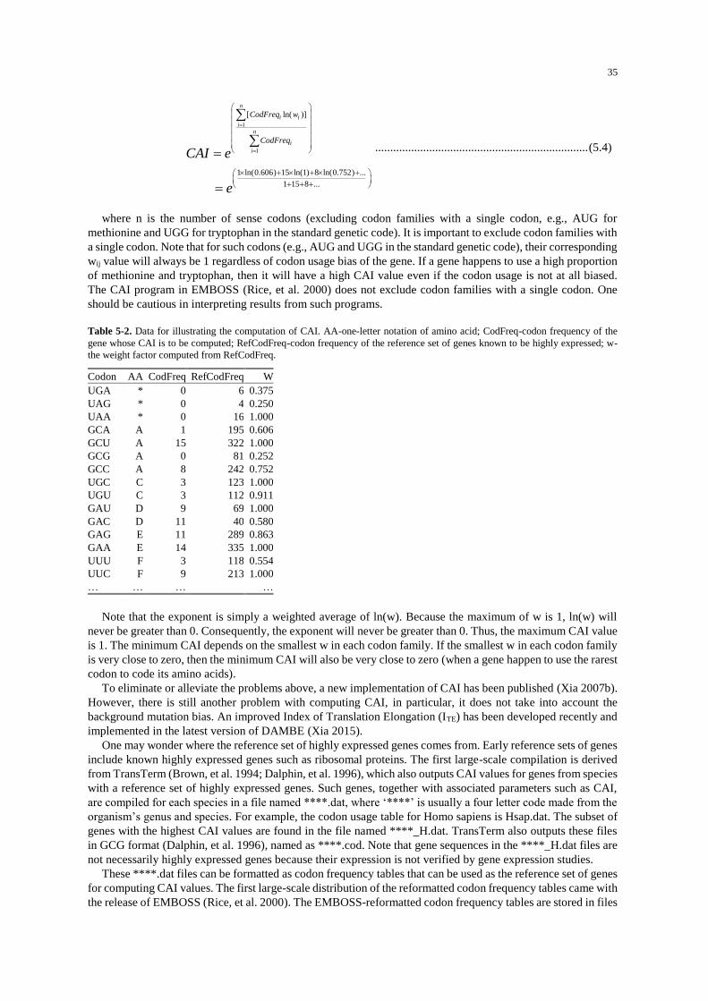
35
1
1
[ ln( )]
1 ln(0.606) 15 ln(1) 8 ln(0.752) ...
1 15 8 ...
n
i i
i
n
i
i
CodFreq w
CodFreq
CAI e
e
....................................................................... (5.4)
where n is the number of sense codons (excluding codon families with a single codon, e.g., AUG for
methionine and UGG for tryptophan in the standard genetic code). It is important to exclude codon families with
a single codon. Note that for such codons (e.g., AUG and UGG in the standard genetic code), their corresponding
wij value will always be 1 regardless of codon usage bias of the gene. If a gene happens to use a high proportion
of methionine and tryptophan, then it will have a high CAI value even if the codon usage is not at all biased.
The CAI program in EMBOSS (Rice, et al. 2000) does not exclude codon families with a single codon. One
should be cautious in interpreting results from such programs.
Table 5-2. Data for illustrating the computation of CAI. AA-one-letter notation of amino acid; CodFreq-codon frequency of the
gene whose CAI is to be computed; RefCodFreq-codon frequency of the reference set of genes known to be highly expressed; w-
the weight factor computed from RefCodFreq.
Codon AA CodFreq RefCodFreq W
UGA * 0 6 0.375
UAG * 0 4 0.250
UAA * 0 16 1.000
GCA A 1 195 0.606
GCU A 15 322 1.000
GCG A 0 81 0.252
GCC A 8 242 0.752
UGC C 3 123 1.000
UGU C 3 112 0.911
GAU D 9 69 1.000
GAC D 11 40 0.580
GAG E 11 289 0.863
GAA E 14 335 1.000
UUU F 3 118 0.554
UUC F 9 213 1.000
… … … …
Note that the exponent is simply a weighted average of ln(w). Because the maximum of w is 1, ln(w) will
never be greater than 0. Consequently, the exponent will never be greater than 0. Thus, the maximum CAI value
is 1. The minimum CAI depends on the smallest w in each codon family. If the smallest w in each codon family
is very close to zero, then the minimum CAI will also be very close to zero (when a gene happen to use the rarest
codon to code its amino acids).
To eliminate or alleviate the problems above, a new implementation of CAI has been published (Xia 2007b).
However, there is still another problem with computing CAI, in particular, it does not take into account the
background mutation bias. An improved Index of Translation Elongation (ITE) has been developed recently and
implemented in the latest version of DAMBE (Xia 2015).
One may wonder where the reference set of highly expressed genes comes from. Early reference sets of genes
include known highly expressed genes such as ribosomal proteins. The first large-scale compilation is derived
from TransTerm (Brown, et al. 1994; Dalphin, et al. 1996), which also outputs CAI values for genes from species
with a reference set of highly expressed genes. Such genes, together with associated parameters such as CAI,
are compiled for each species in a file named ****.dat, where ‘****’ is usually a four letter code made from the
organism’s genus and species. For example, the codon usage table for Homo sapiens is Hsap.dat. The subset of
genes with the highest CAI values are found in the file named ****_H.dat. TransTerm also outputs these files
in GCG format (Dalphin, et al. 1996), named as ****.cod. Note that gene sequences in the ****_H.dat files are
not necessarily highly expressed genes because their expression is not verified by gene expression studies.
These ****.dat files can be formatted as codon frequency tables that can be used as the reference set of genes
for computing CAI values. The first large-scale distribution of the reformatted codon frequency tables came with
the release of EMBOSS (Rice, et al. 2000). The EMBOSS-reformatted codon frequency tables are stored in files
36
named E*.cut where the prefix E is presumably for EMBOSS and the file type “cut” is for codon usage table.
The * part in the file is typically a species designation, but unfortunately is not standardized. Because EMBOSS
is open-source, and consequently because everybody can contribute to it with little restriction, there was an
undesirable proliferation of E*.cut files. For example, you will find Ehum.cut, Ehuman.cut, Eco.cut, Eeco_h.cut,
Eecoli, Emus.cut, etc. In some cases, the species is easy to tell. For example, the first two file names in the
previous sentence refer to human, the next three refer to Escherichia coli, with the middle one referring to highly
expressed E. coli genes (i.e., from genes with high CAI values, not from genes experimentally verified to be
highly expressed), and the last refers to Mus musculus. Names ending with cp refer to chloroplast genes. For
example, Emzecp.cut is from maize chloroplast genes. File names ending with mt are from mitochondrial genes.
For example, Eyscmt.cut is derived from the yeast (Saccharomyces cerevisiae) mitochondrial genes.
There are two major problems with the EMBOSS compilation of reference genes. First, the nonstandard
species designation, coupled with a lack of documentation typically associated with open-source software, has
led to a profound confusion as to which file refers to which species. Second, the reference set of genes are
supposed to be highly expressed, but it is difficult to define highly expressed genes in multicellular eukaryotes
because a gene may be highly expressed only in a certain tissue at a certain time. For these reasons, my laboratory
has initiated a large-scale compilation of tRNA anticodons for each species and uses the frequencies of the
cognate codons as a reference to compute CAI values. This is based on the rationale that a gene with its codon
usage maximizing the use of the most abundant cognate tRNA must be a highly expressed gene (Ikemura 1981b;
Gouy and Gautier 1982; Xia 1998a).
You may have already noted that, in contrast to RSCU which is codon-specific, CAI is gene-specific. It makes
no sense to say that a hemoglobin gene has a RSCU value of 2, neither does it make sense to say that a codon
(e.g., GCU) has a CAI value of 0.8.
Codon usage bias and tRNA abundance
The tRNA sequences are essential in the translation hypothesis. Each tRNA can be viewed as an adaptor with
one end attached to an amino acid and the other end matching the cognate codon. The latter is called the
anticodon loop.
The anticodon in almost all tRNA sequences from all species share the regular feature of being flanked by
two nucleotides on either side to form a loop that is held together by a stem. For example, the anticodon loop
(AC loop) of tRNA-Ala in M. musculus is 24AUUGAUUUGCAUUCAAU40 where the starting and ending
numbers indicate the position of the AC loop in the tRNA sequence (numbered from 1), with the anticodon (5’-
UGC-3’) flanked by two nucleotides on either side (bolded) to form a loop that is held together by a stem made
of the first and the last four nucleotides. Such a regular AC loop and its anticodon can be easily identified by
dynamic programming. A few tRNA sequences have an anticodon flanked by three nucleotides, e.g., tRNA-Val
in Erpetoichthys calabaricus and tRNA-Ser1 in the blue whale, Balaenoptera musculus. Some tRNA sequences
have a suspicious AC loop. For example, the AC loop of tRNA-Trp is 26GAGCCUUCAAAGCCC42 with a
stem that has a mismatch. For such tRNA sequences with an irregular AC loop, DAMBE will flag them out and
we will need to check the sequence manually.
Different tRNA species do not exist in the same amount. Some amino acids have many tRNA species, while
others have few, carrying them. Within the same codon family, e.g., the glycine codon family GGN, some codons
are recognized by more codons than others. In E. coli, GGC and GGU have more tRNAs to translate them than
GGA and GGG. For this reason, highly expressed E. coli genes code almost all glycine residues by GGC and
GGU codons. This increases the rate of translation (Xia 1998a, 2005; Carullo and Xia 2008; Xia 2008).
How would we know the relative abundance of different tRNA species? Fortunately for us, there is a high
correlation between relative tRNA abundance and the copy number of tRNA genes in the genome of prokaryotic
species and unicellular eukaryotes (Ikemura 1992; Percudani, et al. 1997; Kanaya, et al. 1999; Duret 2000). So
we will use the copy number of tRNA genes in the genome as an index of relative tRNA abundance.
In this lab, we will work on E. coli genome. All tRNA genes will be extracted and the anticodon identified
by DAMBE. You will look at the output to find cases where DAMBE may fail to identify the correct codon and
manually identify the anticodon. You may have computed CAI before, but the information on tRNA genes will
greatly enhance our understanding of CAI and codon usage.
37
Objectives
Use RSCU and CAI to characterize codon usage
RSCU is a codon-specific index for codon usage, whereas CAI is a gene-specific index for codon usage. Both
are related to gene expression, especially in prokaryotes and unicellular eukaryotes.
Understand the relationship between tRNA abundance and codon usage
Through a detailed study of tRNA genes in E. coli genome, you will develop a good understanding of the
relationship between relative tRNA abundance and codon usage bias.
Procedures
Computing CAI and RSCU
Read into DAMBE the E. coli CDS sequences saved in a previous laboratory. If you did not have a saved file
containing E. coli CDS sequences, then download the E coli K12 genome in GenBank format by using Entrez,
and save to file EcoliK12.gbk. Start DAMBE, and click ‘File|Open standard sequence file’. In the ‘File of type’
dropdown listbox, choose ‘GenBank file’ format. Choose the saved E. coli file (EcoliK12.gbk) and click the
‘Open’ button. Choose CDS and click ‘OK’. Save the file to your personal directory in FASTA format.
Calculate CAI: Click ‘Seq.Analysis|Codon usage|Codon adaptation index (CAI). A dialog box will be
displayed for you to choose options (Fig. 5-1). The upper panel should display two listboxes with the left
showing sequences available for analysis and the right showing sequences selected to compute CAI. You may
choose one or a subset of sequences and click the '-->' button. In our case, we will compute CAI for all CDSs,
so click the ‘Add all’ button to move all sequences to the right. Leave the ‘Detailed output’ checkbox unchecked
(otherwise it will produce too much output). In ‘Choose a species’ dropdown box, choose ‘Escherichia coli K12
(high) which will use the highly expressed E. coli genes as the reference set. The same reference set of genes
can also be used for any E. coli or Shigella strains because what is highly expressed in E. coli K12 is also almost
always highly expressed in similar strains.
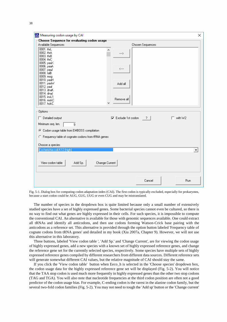
38
Fig. 5-1. Dialog box for computing codon adaptation index (CAI). The first codon is typically excluded, especially for prokaryotes,
because a start codon could be AUG, GUG, UUG or even CUG and may be mistranslated.
The number of species in the dropdown box is quite limited because only a small number of extensively
studied species have a set of highly expressed genes. Some bacterial species cannot even be cultured, so there is
no way to find out what genes are highly expressed in their cells. For such species, it is impossible to compute
the conventional CAI. An alternative is available for those with genomic sequences available. One could extract
all tRNAs and identify all anticodons, and then use codons forming Watson-Crick base pairing with the
anticodons as a reference set. This alternative is provided through the option button labeled 'Frequency table of
cognate codons from tRNA genes' and detailed in my book (Xia 2007a, Chapter 9). However, we will not use
this alternative in this laboratory.
Three buttons, labeled 'View codon table ', 'Add Sp.' and 'Change Current', are for viewing the codon usage
of highly expressed genes, add a new species with a known set of highly expressed reference genes, and change
the reference gene set for the currently selected species, respectively. Some species have multiple sets of highly
expressed reference genes compiled by different researchers from different data sources. Different reference sets
will generate somewhat different CAI values, but the relative magnitude of CAI should stay the same.
If you click the 'View codon table' button when Eeco_h is selected in the 'Choose species' dropdown box,
the codon usage data for the highly expressed reference gene set will be displayed (Fig. 5-2). You will notice
that the TAA stop codon is used much more frequently in highly expressed genes than the other two stop codons
(TAG and TGA). You will also note that nucleotide frequencies at the third codon position are often not a good
predictor of the codon usage bias. For example, C-ending codon is the rarest in the alanine codon family, but the
several two-fold codon families (Fig. 5-2). You may not need to tough the 'Add sp' button or the 'Change current'

39
button until you begin your own research and find your species is either not listed in the dropdown box or listed
with a rather unrepresentative reference set. In that case, you may compile your own reference set of highly
expressed genes so that you can compute CAI with your own reference set of highly expressed genes.
Fig. 5-2. The reference set of highly expressed genes in Escherichia coli (Some genes in the reference may be replaced by others
leading to differences in the actual numbers.
Now that we have gotten thoroughly familiar with the dialog box in Fig. 5-1, click the ‘Run’ button. The CAI
value will be computed for each gene and displayed in the format in Table 5-3. In addition to the conventional
CAI, the slight modification, designated CAI2, is also displayed (Table 5-3). CAI2 is defined as
1
1
[ )]n
i i
i
n
i
i
CodFreq w
CodFreq
(5.5)
which avoids the problem associated with wi = 0. You may ignore it in this lab.
Which three genes have the highest CAI values? Which three the lowest? What are the main differences in
codon usage between those with high CAI values and those with low CAI values? To address these questions,
you should first sort the genes by CAI values. We will do this in EXCEL and take this opportunity to learn how
to get data in DAMBE's display to EXCEL sheet. (Note that CAI is computed with a set of genes known to be
highly expressed. Changing this reference set of genes could also change the CAI values. DAMBE will generally
use the most accurate compilation of highly expressed genes and the CAI values you have may not be the same
as shown here.)
When the CAI is displayed, highlight the output table (Fig. 5-3). Click 'Edit|Copy to EXCEL'. Now launch
EXCEL, click a cell and click the 'Paste' button (or just press Ctrl-V). The table will be copied into EXCEL is
four columns. Now highlight all the data and click 'Data|Sort' in EXCEL to sort the data by CAI.
Table 5-3. Output of CAI for each gene. You may ignore CAI2.
SeqName SeqLen CAI CAI2
thrA 2463 0.55097 0.70581
thrB 933 0.53635 0.70278
thrC 1287 0.60688 0.73973
yaaX 297 0.47696 0.66049
yaaA 777 0.53883 0.68732
yaaJ 1431 0.48754 0.66228

40
talB 954 0.75838 0.83941
mog 588 0.58178 0.72263
… … … …
Fig. 5-3. Transfer tables from DAMBE to EXCEL.
Some genes are very short with few codons. Avoid such genes because they may not be true genes. Even if
they are, the few codons they contain may not reveal any clear patterns. Instead, find three high-CAI genes and
three low-CAI genes with sequence length at least 500 bases long. Click ‘File|Save a subset of sequences’ to
save these six genes with extreme CAI values in FASTA format. These genes will be used to practice the
computation of RSCU.
Calculate RSCU: We want to obtain pooled RSCU for the three high-CAI genes and that for the three low-
CAI genes and compare their differences. Our prediction is that highly expressed genes should maximize, within
each codon family, the usage of codons efficiently translated by tRNAs and minimize the usage of codons that
have few tRNAs to translate them. For this reason, they should have more biased codon usage with RSCU
deviating substantially from 1, than lowly expressed genes with RSCU staying relatively closer to 1. Will this
prediction be supported?
Click ‘File|Read standard sequence file’ to read the FASTA file containing the six genes with extreme CAI
values. Click ‘Seq.Analysis|Codon usage|RSCU’. Click the three high-CAI genes to the right listbox, and then
click the 'Run' button. When the results are displayed, copy and paste the table into another EXCEL sheet. Do
the same for the three low-CAI genes. Table 5-4 shows the results ready for comparison.
Table 5-4. Contrast of RSCU between genes with high CAI value (RSCU_H) and genes with low-CAI value (RSCU_L).
Codon AA ObsFreq RSCU_H Codon AA ObsFreq RSCU_L
UGA * 0 0 UGA * 1 1
UAG * 0 0 UAG * 0 0
UAA * 3 3 UAA * 2 2
GCU A 72 2.549 GCU A 22 1.419
GCG A 14 0.496 GCG A 9 0.581
GCC A 5 0.177 GCC A 7 0.452
GCA A 22 0.779 GCA A 24 1.548
… . .. … … . .. ….
Examine the output for the six genes. With the alanine codon family shown in Table 5-4, we see that genes
with high-CAI have more biased codon usage with highest RSCU being 2.549 for the GCU codon and the lowest
being only 0.177 for the GCC codon. In contrast, for the low-CAI genes, the highest and lowest RSCU is 1.419
and 0.452, spanning a much smaller range.

41
What can you infer about the tRNA carrying alanine? There could be tRNAAla/AGC, tRNAAla/CGC, tRNAAla/GGC,
and tRNAAla/UGC in the E. coli genome. Which tRNAAla species is likely to be the most abundant in E. coli cell?
Given that GCU is the most frequently used codon, we may predict that tRNAAla/AGC may be the most abundant.
How can we test this prediction? It would be nice if we could quantify the abundance of the four tRNAAla species.
Unfortunately this is extremely tedious experimentally. One alternative is based on the observation that tRNA
abundance is highly correlated with the copy number of tRNA genes. So we may predict that the tRNAAla/AGC
gene not only should be present in the E. coli genome, but also have more copies than other tRNAAla species.
An alternative hypothesis, termed wobble versatility hypothesis (Carullo and Xia 2008; Xia 2008; Xia 2013c),
makes predictions differently concerning the tRNA anticodon, based on the assumption that the tRNA anticodon
should maximize its wobble capacity. For four-fold degenerate codon families such as the alanine codon family,
it predicts that there should be tRNAAla/GGC translating GCC and GCU codons and tRNAAla/UGC translating GCA
and GCG codons. Testing these different hypotheses and their predictions obviously would require us to extract
tRNA genes from the E. coli genome and identify the anticodons. We will learn these techniques in the next
section.
The alanine codon family is consistent with our prediction that highly expressed genes should exhibit more
codon usage bias than lowly expressed genes. Is this pattern generally true for other codon families? Fig. 5-4
plots the RSCU for the high-CAI genes (RSCU_H) and the low-CAI genes (RSCU_L) versus the 64 codons. It
is quite clear that high-CAI genes (representing highly expressed genes) have RSCU values deviating much
more from 1 than the low-CAI genes (representing lowly expressed genes). We conclude that highly expressed
genes are under strong selection to maximize translation efficiency and accuracy which has driven their
evolution towards optimizing their codon usage. In contrast, such selection should be weak for lowly expressed
genes whose codon usage may largely depend on mutation bias.
0
0.5
1
1.5
2
2.5
3
3.5
4
4.5
UG
AU
AG
UA
A
GC
UG
CG
GC
C
GC
AU
GU
UG
CG
AU
GA
C
GA
GG
AA
UU
UU
UC
GG
UG
GG
GG
CG
GA
CA
CC
AU
AU
UA
UA
AU
CA
AA
AA
GC
UA
CU
CC
UG
CU
U
UU
A
UU
GA
UG
AA
CA
AU
CC
AC
CC
CC
UC
CG
CA
AC
AG
AG
A
AG
GC
GA
CG
C
CG
GC
GU
AG
CA
GU
UC
A
UC
CU
CG
UC
U
AC
CA
CA
AC
GA
CU
GU
UG
UG
GU
CG
UA
UG
GU
AC
UA
U
Codon
RS
CU
RSCU_H RSCU_L
Fig. 5-4. RSCU for high-CAI and low-CAI genes (RSCU_H and RSCU_L, respectively), plotted over the 64 codons.
Identifying tRNA anticodon
Extract and save tRNA sequences: (If you have not done so already) Download the E. coli K12 substr.
MG1655 genomic sequence (RefSeq: NC_000913) by using Entrez. Save the file to EcoliK12.gbk in your local
directory.
Read EcoliK12.gbk into DAMBE by clicking “File|Open standard sequence file’. In the 'File of type'
dropdown listbox, choose GenBank file format. In the ensuing dialog box prompting you what to extract, choose
tRNA. In the ensuing dialog box asking you to specify the sequence type, choose 'Non-protein-coding'.
When the sequences are displayed, click “File|Save or convert sequences” to save the tRNA sequences to a
file named EcoliK12tRNA.fas.
Note that E. coli K12 contains six identical tRNALys genes and four identical tRNAAsn genes. We will have a
closer look at the effect of these tRNA genes on codon usage bias.
Identify tRNA anticodon by using DAMBE: Click “Seq.Analysis|tRNA anticodon and AC loop”. You will
be asked for a temperature because RNA fold differently in different temperature. For mammalian species or
their parasites and commensals, input 37 (degrees Celcius) which is the default. For avian species and their
parasites/commensals, enter 39. For poikilotherms, a 20 is perhaps a good guess. Click the Yes button to run.
Examine the output. Are all tRNA anticodons identified correctly? How would you know if they are identified
correctly? Note that DAMBE’s identification is based on the sequence only, whereas the GenBank identification

42
is based on much more information. So any discrepancy between DAMBE and GenBank can be assumed to be
a misidentification by DAMBE.
It is important for you to check the result and to learn how to manually identify the AC loop and anticodon.
Suppose a tRNAVal gene has the same sequence
GGGUGAUUAGCUCAGCUGGGAGAGCACCUCCCUUACAAGGAGGGGGUCGGCGGUUCGAUCCC
GUCAUCACCCACCA
The anticodon is typically near the middle of the sequence, and should be flanked by two nucleotides on either
side to form an anticodon loop held together by a stem (Fig. 5-5). If we know that the amino acid carried by the
tRNA, then it is easy to identify the anticodon. For example, valine is coded by GUN, so the anticodon of
tRNAVal should be NAC. There are only two NAC’s in the sequence, but only the second one follows the
anticodon loop structure, i.e., CCUCCCUUACAAGGAGG. Note that the anticodon is flanked by CU on the
5’ side and AA on the 3’ side, and the seven nucleotide anticodon loop is held by a stem formed by base-pairing
between CCUCC and GGAGG. DAMBE is supposed to infer the anticodon from the sequence only, so any five-
nucleotide loop held together by a stem, located somewhere near the center of the sequence, may be taken as a
putative anticodon loop. Do the same manual identification for other tRNA sequences that might have a
misidentified anticodon loop.
UCC
3’-AGG-5’
5’ 3’
G-C
C-G
U-A
G-C
A-UC
U Anticodon
A
A
Codon (Gly)
Fig. 5-5. Anticodon loop of tRNAGly/UCC.
Note that E. coli K12 contains six identical tRNALys genes with anticodon UUU forming Watson-Crick base-
pair with the AAA codon. Lysine is coded by a two-fold codon family with AAA and AAG codons. Given that
all tRNALys genes have the anticodon pairing with the AAA codon, we should expect AAA codon to be used
more frequently than AAG codons. Although the wobble U in the tRNA anticodon can also pair with G in RNA
secondary structure, such U/G base-pair is considered energetically less favorable than U/A pair, i.e., we should
expect the AAA codon to be used more often to code lysine than the AAG codon. Check your RSCU results for
the high-CAI genes to see if this is true. If the AAG codon is used just as frequently as the AAA codon, then our
assumption that U/A is energetically more favorable than U/G pair may be wrong.
Also note that E. coli K12 has four identical tRNAAsn genes all with anticodon GUU forming Watson-Crick
base-pair with AAC codons. Asparagine is coded by a two-fold codon family with AAC and AAU codons.
Given that all tRNAAsn genes have the anticodon pairing with the AAC codon, we should expect AAC codon to
be used more frequently than AAU codons. Although the wobble G in the anticodon can pair with both C and
U in RNA secondary structure, such U/G base-pair is considered energetically less favorable than U/A pair, i.e.,
we should expect the AAC codon to be used more often to codon lysine than the AAU codon. Check your RSCU
results for the high-CAI genes to see if this is true. If the AAG codon is used just as frequently as the AAA
codon, then our assumption that U/A is energetically more favorable than U/G pair may be wrong.
Look at other tRNAs and other codon families and find exceptions to this rule of codon-anticodon adaptation.
Discuss with each other, or ask me or a TA, to find answers to such exceptions. Remember that a good scientist
can explain all the commonly observed phenomena in his field, but only a great scientist can also explain rare
and exceptional phenomena.
More questions
1. Someone states that the pig hemoglobin gene has a RSCU value of 2. Does it make sense to you?
2. Someone states that the GGA codon of the pig hemoglobin gene has a CAI value of 0.75. Does it make
sense?
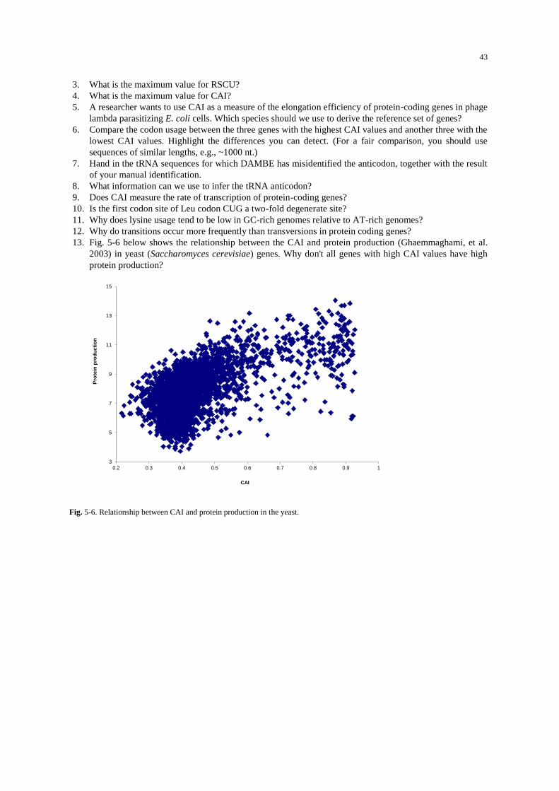
43
3. What is the maximum value for RSCU?
4. What is the maximum value for CAI?
5. A researcher wants to use CAI as a measure of the elongation efficiency of protein-coding genes in phage
lambda parasitizing E. coli cells. Which species should we use to derive the reference set of genes?
6. Compare the codon usage between the three genes with the highest CAI values and another three with the
lowest CAI values. Highlight the differences you can detect. (For a fair comparison, you should use
sequences of similar lengths, e.g., ~1000 nt.)
7. Hand in the tRNA sequences for which DAMBE has misidentified the anticodon, together with the result
of your manual identification.
8. What information can we use to infer the tRNA anticodon?
9. Does CAI measure the rate of transcription of protein-coding genes?
10. Is the first codon site of Leu codon CUG a two-fold degenerate site?
11. Why does lysine usage tend to be low in GC-rich genomes relative to AT-rich genomes?
12. Why do transitions occur more frequently than transversions in protein coding genes?
13. Fig. 5-6 below shows the relationship between the CAI and protein production (Ghaemmaghami, et al.
2003) in yeast (Saccharomyces cerevisiae) genes. Why don't all genes with high CAI values have high
protein production?
Fig. 5-6. Relationship between CAI and protein production in the yeast.
3
5
7
9
11
13
15
0.2 0.3 0.4 0.5 0.6 0.7 0.8 0.9 1
Pro
tein
pro
du
cti
on
CAI
44
LAB 6 RNA SECONDARY STRUCTURE, MINIMUM FOLDING
ENERGY, AND IRES
Introduction
Biological functions of nucleotide and protein sequences are often related to their secondary structure. Whether
a transcribed “tRNA” sequence is functional depends on whether it can be folded into proper structure. Different
mRNAs have different 5’ UTRs that often differ dramatically in their efficiency in loading ribosomes onto the
mRNA, leading to different translation initiation efficiency and protein production. This difference is often
related to the secondary structure that form at the 5’ end of the mRNAs (Zid, et al. 2009). Some genes are
transcribed but translated only under special circumstances. For example, some yeast genes are transcribed but
only translated under nutrient depletion to help the yeast to find new nutrient sources. This is achieved by their
unique secondary structure (or the shared lack of secondary structure) in the 5’ UTR or these genes (Gilbert, et
al. 2007; Xia and Holcik 2009). As efficient protein production directly affects the profit of biopharmaceutical
industry, optimization of the 5’ UTR, especially its secondary structure, represents research efforts of many
biopharmaceutical industry including the production of vaccines which needs to be produced in large quantity
in a short time in response to emerging infective agents such as Influenza viruses. For this reason, characterizing
secondary structure is a crucial bioinformatic skill useful in a variety of circumstances.
RNA secondary structure
RNA molecules, e.g., tRNA, rRNA, mRNA, siRNA, snRNA, etc., typically need to fold into secondary and
tertiary structures to perform their biological function. The 5’ UTR of many mRNA in eukaryotic species or
viral pathogens of eukaryotic cells often contain particular sequences that allow translation initiation by internal
ribosomal entry without involving cap-dependent scanning mechanism. The sequences in 5’ UTR of mRNA that
facilitate internal ribosomal entry are known as internal ribosomal entry sites (IRESs). While many viral IRESs
are known to contain special secondary structures, many eukaryotic IRESs are devoid of secondary structure.
The secondary structure of RNA molecules are formed by three kinds of base-paring, G/C, A/U and G/U,
with the G/U being the weakest, leading to what is called a stem-loop structure. Functional RNA molecules in
bacteria living in hot springs typically have higher percentage of GC and more G/C pairs than RNA in bacterial
species living in habitats with a low temperature. This contrast is particularly strong at the stem region, which
makes sense because it is mainly the stem that maintains the secondary structure. RNAs from organisms in high
temperature also have longer stems than that from organisms in low temperature.
Minimum folding energy (MFE)
The stability of secondary structure formed by an RNA is typically measured by minimum folding energy
(MFE), which is expressed as the amount of energy required to break the secondary structure. The more negative
MFE is, the more stable the secondary structure.
It is important to keep in mind that the structure of any macromolecule is almost always dynamic instead of
static. It is like the walk of a drunkard along a trail, jerking left and right but still is most likely to stay in the
middle of the trail. However, the probability that we will actually observe him right in the middle of the road at
any particular time point is quite small. Similarly, an RNA molecular will jerk into non-minimum-energy states
quite often.
5’ UTR secondary structure and translation economy
While the filthy rich can afford a great deal of wasteful expenditure, a pauper would have to economize his
budget. The same principle applies to cellular and subcellular systems. For example, a 5’ UTR with a strong
secondary structure will require eIF-4A or equivalent helicases to unwind such secondary structure. When
nutrient is unlimited and ATP is plenty, such ATP-consuming unwinding is not a serious problem. However,
when nutrient is limited and ATP is scarce, a 5’ UTR with a strong secondary structure would become wasteful.
One can immediately derive a prediction from this hypothesis. That is, when nutrient is limited, mRNAs with
increased translation should have 5’ UTRs with weak secondary structure, whereas mRNAs with strong
secondary structure should exhibit dramatically reduced translation. Zid et al (2009) tested this prediction by
using DAMBE to calculate MFE of the 5’ UTR of translationally up- and down-regulated mRNA in nutrient
limited Drosophila melanogaster. The result strongly supported the prediction. Translation of mRNAs that have
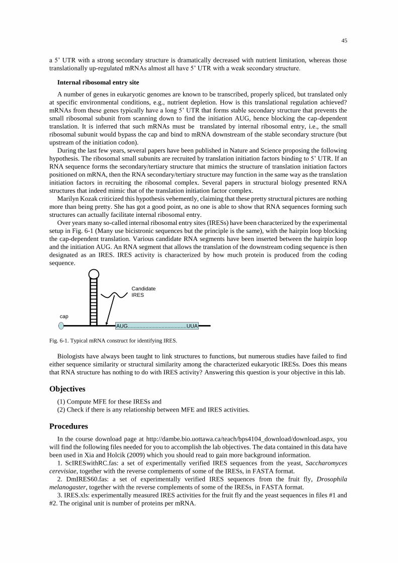
45
a 5’ UTR with a strong secondary structure is dramatically decreased with nutrient limitation, whereas those
translationally up-regulated mRNAs almost all have 5’ UTR with a weak secondary structure.
Internal ribosomal entry site
A number of genes in eukaryotic genomes are known to be transcribed, properly spliced, but translated only
at specific environmental conditions, e.g., nutrient depletion. How is this translational regulation achieved?
mRNAs from these genes typically have a long 5’ UTR that forms stable secondary structure that prevents the
small ribosomal subunit from scanning down to find the initiation AUG, hence blocking the cap-dependent
translation. It is inferred that such mRNAs must be translated by internal ribosomal entry, i.e., the small
ribosomal subunit would bypass the cap and bind to mRNA downstream of the stable secondary structure (but
upstream of the initiation codon).
During the last few years, several papers have been published in Nature and Science proposing the following
hypothesis. The ribosomal small subunits are recruited by translation initiation factors binding to 5’ UTR. If an
RNA sequence forms the secondary/tertiary structure that mimics the structure of translation initiation factors
positioned on mRNA, then the RNA secondary/tertiary structure may function in the same way as the translation
initiation factors in recruiting the ribosomal complex. Several papers in structural biology presented RNA
structures that indeed mimic that of the translation initiation factor complex.
Marilyn Kozak criticized this hypothesis vehemently, claiming that these pretty structural pictures are nothing
more than being pretty. She has got a good point, as no one is able to show that RNA sequences forming such
structures can actually facilitate internal ribosomal entry.
Over years many so-called internal ribosomal entry sites (IRESs) have been characterized by the experimental
setup in Fig. 6-1 (Many use bicistronic sequences but the principle is the same), with the hairpin loop blocking
the cap-dependent translation. Various candidate RNA segments have been inserted between the hairpin loop
and the initiation AUG. An RNA segment that allows the translation of the downstream coding sequence is then
designated as an IRES. IRES activity is characterized by how much protein is produced from the coding
sequence.
AUG........................................UUA
cap
Candidate
IRES
Fig. 6-1. Typical mRNA construct for identifying IRES.
Biologists have always been taught to link structures to functions, but numerous studies have failed to find
either sequence similarity or structural similarity among the characterized eukaryotic IRESs. Does this means
that RNA structure has nothing to do with IRES activity? Answering this question is your objective in this lab.
Objectives
(1) Compute MFE for these IRESs and
(2) Check if there is any relationship between MFE and IRES activities.
Procedures
In the course download page at http://dambe.bio.uottawa.ca/teach/bps4104_download/download.aspx, you
will find the following files needed for you to accomplish the lab objectives. The data contained in this data have
been used in Xia and Holcik (2009) which you should read to gain more background information.
1. ScIRESwithRC.fas: a set of experimentally verified IRES sequences from the yeast, Saccharomyces
cerevisiae, together with the reverse complements of some of the IRESs, in FASTA format.
2. DmIRES60.fas: a set of experimentally verified IRES sequences from the fruit fly, Drosophila
melanogaster, together with the reverse complements of some of the IRESs, in FASTA format.
3. IRES.xls: experimentally measured IRES activities for the fruit fly and the yeast sequences in files #1 and
#2. The original unit is number of proteins per mRNA.

46
You access the MFE function in DAMBE by clicking ‘Structure|RNA minimum folding energy’. You are on
your own to choose the options, but you need to justify what you have chosen in the assignment below. The unit
for MFE is KJ/mol.
Assignment
Write a mini-manuscript. Outline in the “Introduction” section the objective of testing if there is any relationship
between MFE and IRES activities. The manuscript, including “Methods”, “Results”, “Discussion” and
“References” sections, should be no more than three pages (single-spaced. The “References” section will not be
counted towards the page limit). You may include tables and graphs which also will not be counted towards the
page limit. You may read Xia and Holcik (2009) to gain more background information.
47
LAB 7 PROTEIN ISOELECTRIC POINT AND ACID-RESISTANCE
Introduction
Proteins are the workhorses in a living cell. They can perform a variety of tasks because of their diverse
properties. Isoelectric point is just one of many properties of proteins. Although we focus on isoelectric point in
this laboratory, the same large-scale comparative studies illustrated in this laboratory can be performed on other
properties as well.
Protein isoelectric point
The isoelectric point of a protein can often determine the cellular localization and function of the protein, and
needs to be characterized in order to understand its molecular biology or pharmaceutical properties. Proteins
binding to RNA and DNA often have a positively charged domain forming nonspecific electrostatic interaction
with the negative phosphate backbone of nucleotide acids. This is true for nearly all transcription factors.
Positively charged peptides and proteins under physiological pH can be readily taken up by the liver and kidney.
Thus, a protein drug intended for liver or kidney diseases should be designed to be positively charged. Positively
charged peptides and proteins can also cross the blood-brain barrier by a mechanism related to receptor-mediated
transcytosis (Terasaki, et al. 1991; Tamai, et al. 1997). Thus, a protein drug intended for the brain should be
positively charged, but should not be taken up or degraded by the liver or the kidney.
The isoelectric point of a protein is determined by its ionizable groups such as carboxyl groups and amino
groups. Since the charge of these groups depends on pH, a protein molecule can have different charges according
to pH. The pH at which the number of negative charges is the same as the number of positive charges of the
protein molecule is the isoelectric point of the protein, i.e., the pH at which the protein carries no net charge.
Isoelectric point is typically abbreviated as pI.
A protein will carry positive charges if its pI is greater than its physiological pH, and negative charge is its pI
is smaller than its physiological pH. The electrostatic repulsion between proteins is smallest at this point and the
solubility is consequently the lowest. Proteins with low solubility may aggregate and precipitate which is often
bad for the cell. The “amyloid precursor protein” causing Alzheimer disease and the prion protein causing the
mad cow disease are examples of the undesirable protein aggregation and precipitation.
If an organism has its cellular pH at 7, should its proteins, especially those mass-produced ones, have
isoelectric point at 7? What distribution of protein isoelectric points would you expect to find in Escherichia
coli that live in the intestine with its environmental pH about 8-9? What about Helicobacter pylori which lives
in the acidic environment of mammalian stomach?
Acid-resistance in Helicobacter pylori and its protein isoelectric point
Helicobacter pylori (Fig. 7-1) is a human pathogen causing gastric and duodenal ulcers and gastric cancer
(Hamajima, et al. 2004; Hunt 2004; Menaker, et al. 2004; Siavoshi, et al. 2004). It is an acid-resistant
neutralophile (Scott, et al. 2002) capable of surviving for at least 3 hours at pH 1 with urea (Stingl, et al. 2001)
and maintaining a nearly neutral cytoplasmic pH between pH 3.0 and 7.0 (Matin, et al. 1996; Scott, et al. 2002;
Stingl, Uhlemann, et al. 2002). These properties allow it to resist the acid shock in human gastric fluid that has
a pH averaging about 1.4 over a 24-h period (Sachs, et al. 2003) and infect the gastric mucosa. The buffering
action of the gastric epithelium and limited acid diffusion through the gastric mucus was previously thought to
protect the bacterium against stomach acidity, but both empirical studies (Allen, et al. 1993) and theoretical
modeling (Engel, et al. 1984) have suggested that the protection is rather limited (Matin, et al. 1996). Recently
it has also been shown that mucus does not hinder proton diffusion and a trans-mucus pH gradient is abolished
when the luminal pH drops to < 2.5 (Baumgartner and Montrose 2004). It is therefore necessary for H. pylori to
have acid acclimation mechanisms to colonize the gastric mucosa successfully (Sachs, et al. 2003).
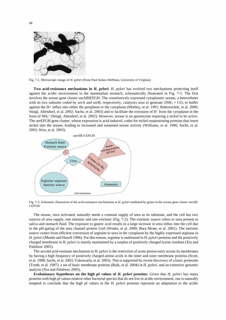
48
Fig. 7-1. Microscopic image of H. pylori (From Paul Stokes Hoffman, University of Virginia).
Two acid-resistance mechanisms in H. pylori: H. pylori has evolved two mechanisms protecting itself
against the acidic environment in the mammalian stomach, schematically illustrated in Fig. 7-2. The first
involves the urease gene cluster ureABIEFGH. The constitutively expressed cytoplasmic urease, a heterodimer
with its two subunits coded by ureA and ureB, respectively, catalyzes urea to generate 2NH3 + CO2 to buffer
against the H+ influx into either the periplasm or the cytoplasm (Mobley, et al. 1991; Rektorschek, et al. 2000;
Stingl, Altendorf, et al. 2002; Sachs, et al. 2003) and to facilitate the extrusion of H+ from the cytoplasm in the
form of NH4+ (Stingl, Altendorf, et al. 2002). However, urease is an apoenzyme requiring a nickel to be active.
The ureEFGH gene cluster, whose expression is acid-induced, codes for nickel-sequestrating proteins that insert
nickel into the urease, leading to increased and sustained urease activity (Williams, et al. 1996; Sachs, et al.
2003; Wen, et al. 2003).
Urease (A+B)
apoenzyme
Urea
Ammonia
Stomach fluid:
Extrinsic source
Arginine+arginase:
Intrinsic source
ureAB-I-EFGH
Nickel-
inserting proteins
(EFGH)I
Cell membrane
Fig. 7-2. Schematic illustration of the acid-resistance mechanisms in H. pylori mediated by genes in the urease gene cluster ureAB-
I-EFGH.
The urease, once activated, naturally needs a constant supply of urea as its substrate, and the cell has two
sources of urea supply, one intrinsic and one extrinsic (Fig. 7-2). The extrinsic source refers to urea present in
saliva and stomach fluid. The exposure to gastric acid results in a large increase in urea influx into the cell due
to the pH-gating of the urea channel protein UreI (Weeks, et al. 2000; Bury-Mone, et al. 2001). The intrinsic
source comes from efficient conversion of arginine to urea in the cytoplasm by the highly expressed arginase in
H. pylori (Mendz and Hazell 1996). For this reason, arginine is underused in H. pylori proteins and the positively
charged membrane in H. pylori is mainly maintained by a surplus of positively charged lysine residues (Xia and
Palidwor 2005).
The second acid-resistant mechanism in H. pylori is the restriction of acute proton entry across its membranes
by having a high frequency of positively charged amino acids in the inner and outer membrane proteins (Scott,
et al. 1998; Sachs, et al. 2003; Valenzuela, et al. 2003). This is supported by recent discovery of a basic proteome
(Tomb, et al. 1997), a set of basic membrane proteins (Baik, et al. 2004) in H. pylori, and an extensive genomic
analysis (Xia and Palidwor 2005).
Evolutionary hypotheses on the high pI values of H. pylori proteins: Given that H. pylori has many
proteins with high pI values relative other bacterial species that do not live in acidic environment, one is naturally
tempted to conclude that the high pI values in the H. pylori proteins represent an adaptation to the acidic

49
environment. However, there are at least four possible hypotheses for the origin of the basic proteome in H.
pylori (Xia 2007a, Chapter 10).
The first hypothesis invokes natural selection and adaptation, i.e., H. pylori inhabits the acidic environment
in mammalian stomach with a high concentration of H+ that may get into the cytoplasm and disrupt cellular pH
homeostasis. So H. pylori needs a lot of positively charged proteins (especially membrane proteins) to alleviate
the influx of H+ into cytoplasm. It is therefore beneficial for the organism to accumulate basic amino acid
residues in its proteins, especially in its membrane proteins. This hypothesis is known as the acid-adaptation
hypothesis (Xia and Palidwor 2005), i.e., H. pylori acquired its high-pI proteins as an adaptation in response to
the acidic environment.
The second hypothesis argues that parasitic bacterial genomes typically evolve towards AT-richness because
spontaneous mutations are generally AT-biased based on comparisons between pseudogenes and their functional
counterparts (Li, et al. 1981; Gojobori, et al. 1982; Li 1983). H. pylori has a relatively AT-rich genome, e.g., the
genomic GC% of H. pylori 26695 is only 38%, in contrast to the genomic GC% of 50% in E. coli substr DH10B.
This potentially mutation-mediated AT-richness will lead to an increase in A-rich codons such as the lysine
codon AAA and AAG (and a consequently increased usage of lysine). The increased lysine usage in proteins
then increases protein pI. Because H. pylori and its sibling species are all parasites, their most recent common
ancestor might have already practiced parasitism and acquired AT-richness and increased frequency of lysine
codons before it became a parasite in the mammalian stomach. Therefore, with an overrepresentation of it lysine
residues in its proteins, it is already pre-adapted to acidic environment. This hypothesis is termed exaptation
hypothesis (Xia and Palidwor 2005), i.e., the process in which an originally neutral trait has subsequently
acquired a beneficial function. A well known example of exaptation is the brain-specific RNA gene BC200
resulting from the exaptation of a presumably neutral SINE repeat (Smit 1999).
The third hypothesis states that nucleotide C is rare in mammalian cells and a mammalian parasite should
therefore minimize the usage of C as a building block of its RNA and DNA. Minimizing C in an organism with
a DNA genome has the necessary consequence of reduced G, with a consequent increase in A and T. This will
also contribute to increase AT and increased lysine codon. Thus, originally an adaptation to a C-rare environment
predisposed the organism to tolerate an acidic environment. Such a mechanism is called preadaptation in
evolution (Xia and Palidwor 2005), i.e., a trait originally selected for one function but that subsequently gained
a different function beneficial to the carrier of the trait. An often cited example of preadaptation is the
rudimentary feather that presumably has been selected for thermoregulation in nonavian dinosaurs but
preadapted their carriers to subsequent evolution of flight.
The fourth hypothesis is more complicated. As mentioned previously, a protein in a solution with a pH equal
to the protein pI is not charged. If highly expressed proteins happen to have their pI equal to the cytoplasmic pH,
then there is no electrostatic repulsion among these proteins when they are mass-produced. Because the proteins
are not charged, their solubility is at the lowest, and they may aggregate and precipitate, which is often harmful
to the cell. The “amyloid precursor protein” causing Alzheimer disease and the prion protein causing the mad
cow disease are examples of the undesirable protein aggregation and precipitation. H. pylori living in an acidic
environment maintains its cytoplasmic pH around 5. This suggests that H. pylori proteins should avoid having
pI = 5. It is biochemically and evolutionarily easier for H. pylori proteins to shift their pI upwards than
downwards. Hence the increase in protein pI overall.
Objectives
Compare pI profiles between Escherichia coli and H. pylori
Proteins have many different properties and isoelectric point is one of them. E. coli thrives in a slightly basic
environment in mammalian intestine, whereas H. pylori is a pathogen inhabiting the strongly acidic environment
of mammalian stomach. Characterizing genomic and proteomic differences between different organisms and
interpreting the difference with reference to their respective environment belong to the field of comparative and
functional genomics/proteomics.
The word ‘proteome’ has been used in two different meanings: (1) the collection of all protein sequences
coded in the genome of an organism, and (2) the collection of all proteins found in a cell type at a specific time.
In the first, a proteome is a genomic property and does not change over developmental time or differ among
different cell types (unless there are mutations). In contrast, in the second, a proteome is a cellular property and
changes over developmental time and typically differ among different cell types. In this laboratory, the word
proteome means the genome-encoded proteome.
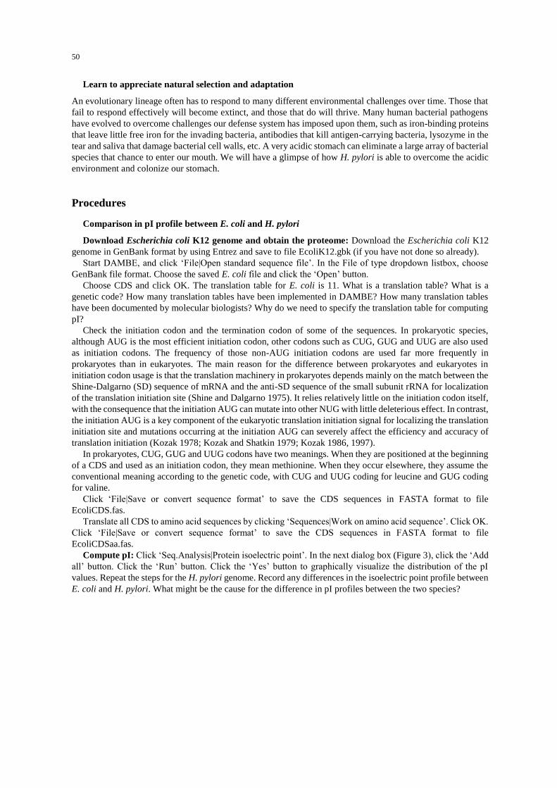
50
Learn to appreciate natural selection and adaptation
An evolutionary lineage often has to respond to many different environmental challenges over time. Those that
fail to respond effectively will become extinct, and those that do will thrive. Many human bacterial pathogens
have evolved to overcome challenges our defense system has imposed upon them, such as iron-binding proteins
that leave little free iron for the invading bacteria, antibodies that kill antigen-carrying bacteria, lysozyme in the
tear and saliva that damage bacterial cell walls, etc. A very acidic stomach can eliminate a large array of bacterial
species that chance to enter our mouth. We will have a glimpse of how H. pylori is able to overcome the acidic
environment and colonize our stomach.
Procedures
Comparison in pI profile between E. coli and H. pylori
Download Escherichia coli K12 genome and obtain the proteome: Download the Escherichia coli K12
genome in GenBank format by using Entrez and save to file EcoliK12.gbk (if you have not done so already).
Start DAMBE, and click ‘File|Open standard sequence file’. In the File of type dropdown listbox, choose
GenBank file format. Choose the saved E. coli file and click the ‘Open’ button.
Choose CDS and click OK. The translation table for E. coli is 11. What is a translation table? What is a
genetic code? How many translation tables have been implemented in DAMBE? How many translation tables
have been documented by molecular biologists? Why do we need to specify the translation table for computing
pI?
Check the initiation codon and the termination codon of some of the sequences. In prokaryotic species,
although AUG is the most efficient initiation codon, other codons such as CUG, GUG and UUG are also used
as initiation codons. The frequency of those non-AUG initiation codons are used far more frequently in
prokaryotes than in eukaryotes. The main reason for the difference between prokaryotes and eukaryotes in
initiation codon usage is that the translation machinery in prokaryotes depends mainly on the match between the
Shine-Dalgarno (SD) sequence of mRNA and the anti-SD sequence of the small subunit rRNA for localization
of the translation initiation site (Shine and Dalgarno 1975). It relies relatively little on the initiation codon itself,
with the consequence that the initiation AUG can mutate into other NUG with little deleterious effect. In contrast,
the initiation AUG is a key component of the eukaryotic translation initiation signal for localizing the translation
initiation site and mutations occurring at the initiation AUG can severely affect the efficiency and accuracy of
translation initiation (Kozak 1978; Kozak and Shatkin 1979; Kozak 1986, 1997).
In prokaryotes, CUG, GUG and UUG codons have two meanings. When they are positioned at the beginning
of a CDS and used as an initiation codon, they mean methionine. When they occur elsewhere, they assume the
conventional meaning according to the genetic code, with CUG and UUG coding for leucine and GUG coding
for valine.
Click ‘File|Save or convert sequence format’ to save the CDS sequences in FASTA format to file
EcoliCDS.fas.
Translate all CDS to amino acid sequences by clicking ‘Sequences|Work on amino acid sequence’. Click OK.
Click ‘File|Save or convert sequence format’ to save the CDS sequences in FASTA format to file
EcoliCDSaa.fas.
Compute pI: Click ‘Seq.Analysis|Protein isoelectric point’. In the next dialog box (Figure 3), click the ‘Add
all’ button. Click the ‘Run’ button. Click the ‘Yes’ button to graphically visualize the distribution of the pI
values. Repeat the steps for the H. pylori genome. Record any differences in the isoelectric point profile between
E. coli and H. pylori. What might be the cause for the difference in pI profiles between the two species?
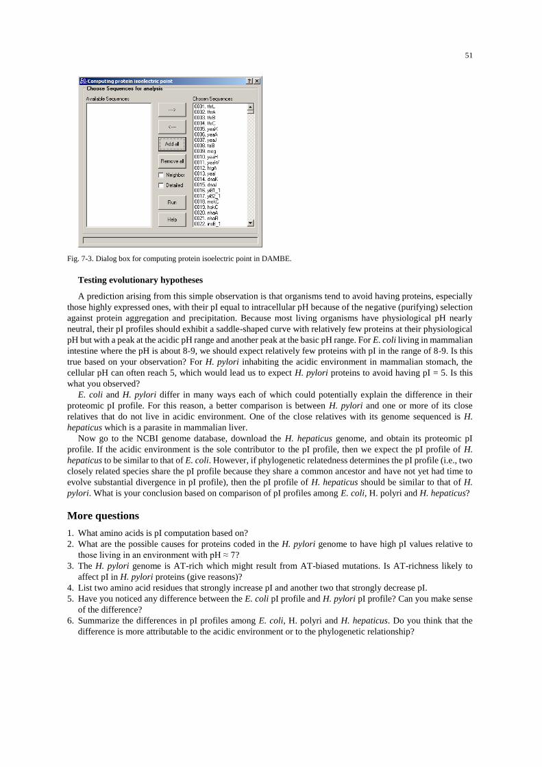
51
Fig. 7-3. Dialog box for computing protein isoelectric point in DAMBE.
Testing evolutionary hypotheses
A prediction arising from this simple observation is that organisms tend to avoid having proteins, especially
those highly expressed ones, with their pI equal to intracellular pH because of the negative (purifying) selection
against protein aggregation and precipitation. Because most living organisms have physiological pH nearly
neutral, their pI profiles should exhibit a saddle-shaped curve with relatively few proteins at their physiological
pH but with a peak at the acidic pH range and another peak at the basic pH range. For E. coli living in mammalian
intestine where the pH is about 8-9, we should expect relatively few proteins with pI in the range of 8-9. Is this
true based on your observation? For H. pylori inhabiting the acidic environment in mammalian stomach, the
cellular pH can often reach 5, which would lead us to expect H. pylori proteins to avoid having pI = 5. Is this
what you observed?
E. coli and H. pylori differ in many ways each of which could potentially explain the difference in their
proteomic pI profile. For this reason, a better comparison is between H. pylori and one or more of its close
relatives that do not live in acidic environment. One of the close relatives with its genome sequenced is H.
hepaticus which is a parasite in mammalian liver.
Now go to the NCBI genome database, download the H. hepaticus genome, and obtain its proteomic pI
profile. If the acidic environment is the sole contributor to the pI profile, then we expect the pI profile of H.
hepaticus to be similar to that of E. coli. However, if phylogenetic relatedness determines the pI profile (i.e., two
closely related species share the pI profile because they share a common ancestor and have not yet had time to
evolve substantial divergence in pI profile), then the pI profile of H. hepaticus should be similar to that of H.
pylori. What is your conclusion based on comparison of pI profiles among E. coli, H. polyri and H. hepaticus?
More questions
1. What amino acids is pI computation based on?
2. What are the possible causes for proteins coded in the H. pylori genome to have high pI values relative to
those living in an environment with pH ≈ 7?
3. The H. pylori genome is AT-rich which might result from AT-biased mutations. Is AT-richness likely to
affect pI in H. pylori proteins (give reasons)?
4. List two amino acid residues that strongly increase pI and another two that strongly decrease pI.
5. Have you noticed any difference between the E. coli pI profile and H. pylori pI profile? Can you make sense
of the difference?
6. Summarize the differences in pI profiles among E. coli, H. polyri and H. hepaticus. Do you think that the
difference is more attributable to the acidic environment or to the phylogenetic relationship?
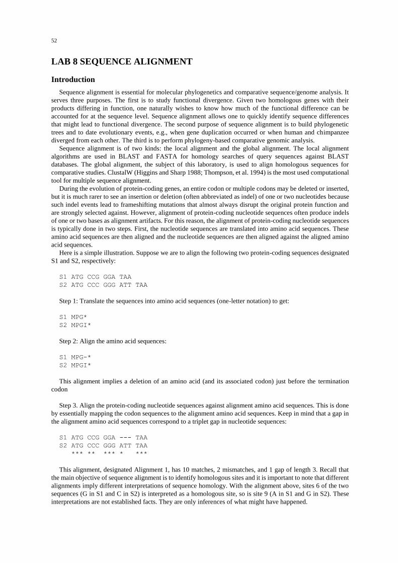
52
LAB 8 SEQUENCE ALIGNMENT
Introduction
Sequence alignment is essential for molecular phylogenetics and comparative sequence/genome analysis. It
serves three purposes. The first is to study functional divergence. Given two homologous genes with their
products differing in function, one naturally wishes to know how much of the functional difference can be
accounted for at the sequence level. Sequence alignment allows one to quickly identify sequence differences
that might lead to functional divergence. The second purpose of sequence alignment is to build phylogenetic
trees and to date evolutionary events, e.g., when gene duplication occurred or when human and chimpanzee
diverged from each other. The third is to perform phylogeny-based comparative genomic analysis.
Sequence alignment is of two kinds: the local alignment and the global alignment. The local alignment
algorithms are used in BLAST and FASTA for homology searches of query sequences against BLAST
databases. The global alignment, the subject of this laboratory, is used to align homologous sequences for
comparative studies. ClustalW (Higgins and Sharp 1988; Thompson, et al. 1994) is the most used computational
tool for multiple sequence alignment.
During the evolution of protein-coding genes, an entire codon or multiple codons may be deleted or inserted,
but it is much rarer to see an insertion or deletion (often abbreviated as indel) of one or two nucleotides because
such indel events lead to frameshifting mutations that almost always disrupt the original protein function and
are strongly selected against. However, alignment of protein-coding nucleotide sequences often produce indels
of one or two bases as alignment artifacts. For this reason, the alignment of protein-coding nucleotide sequences
is typically done in two steps. First, the nucleotide sequences are translated into amino acid sequences. These
amino acid sequences are then aligned and the nucleotide sequences are then aligned against the aligned amino
acid sequences.
Here is a simple illustration. Suppose we are to align the following two protein-coding sequences designated
S1 and S2, respectively:
S1 ATG CCG GGA TAA
S2 ATG CCC GGG ATT TAA
Step 1: Translate the sequences into amino acid sequences (one-letter notation) to get:
S1 MPG*
S2 MPGI*
Step 2: Align the amino acid sequences:
S1 MPG-*
S2 MPGI*
This alignment implies a deletion of an amino acid (and its associated codon) just before the termination
codon
Step 3. Align the protein-coding nucleotide sequences against alignment amino acid sequences. This is done
by essentially mapping the codon sequences to the alignment amino acid sequences. Keep in mind that a gap in
the alignment amino acid sequences correspond to a triplet gap in nucleotide sequences:
S1 ATG CCG GGA --- TAA
S2 ATG CCC GGG ATT TAA
*** ** *** * ***
This alignment, designated Alignment 1, has 10 matches, 2 mismatches, and 1 gap of length 3. Recall that
the main objective of sequence alignment is to identify homologous sites and it is important to note that different
alignments imply different interpretations of sequence homology. With the alignment above, sites 6 of the two
sequences (G in S1 and C in S2) is interpreted as a homologous site, so is site 9 (A in S1 and G in S2). These
interpretations are not established facts. They are only inferences of what might have happened.

53
Aligning protein-coding nucleotide sequences against aligned amino acid sequences assumes that all
sequences are from functional genes. So the minimum requirement for carrying out this procedure is that there
is no embedded stop codon in the sequence.
What is the negative aspect of this approach? What would you miss if the frameshifting mutations actually
happened and the protein-coding gene is still functional? (Hint: if two homologous protein-coding sequences
differ by a frameshifting mutation, then there will always be a fragment of the protein sequences with no
meaningful alignment.)
Depending on the scoring scheme, a nucleotide-based sequence alignment, i.e., without using aligned amino
acid sequences as a mapping reference, may well generate the following alignment designated Alignment 2,
with 12 matches, 0 mismatch and two gaps of lengths 1 and 2, respectively:
S1 ATG CC- GGG A-- TAA
S2 ATG CCC GGG ATT TAA
*** ** *** * ***
Note three different interpretations of the homologous sites between Alignment 1 and Alignment 2. First, the
nucleotide G at site 6 of S1 is now interpreted to be homologous to the nucleotide G at site 7 of S2. Second, the
nucleotide A at site 9 of S1 is now interpreted as homologous to the nucleotide A at site 10 of S2. Which of the
two alignments makes more sense to you? (Hint: Is it likely for a protein-coding gene to remain functional after
two consecutive frameshifting indel mutations?)
If Alignment 1 is correct but we used a nucleotide-based alignment method and end up with Alignment 2,
then the estimation of the genetic distance between the two sequences will be biased. The genetic distance
measures the evolutionary dissimilarity between two sequences, often estimated by ignoring the indel sites. It is
an index of the sequence divergence time used frequently in molecular phylogenetics. In this particular case, if
we perform site-wise deletion of indels, then S1 and S2 would appear more similar to each other for Alignment
2 than for Alignment 1. Biased estimation of the genetic distance often results in failure in molecular
phylogenetic reconstruction (which will be covered in later laboratories).
For sequence alignment involving RNA genes, it is often necessary to incorporate information on the
secondary structure to aid the alignment (Xia 2000; Xia, et al. 2003). However, this is a bit too complicated and
will not be practiced in this laboratory.
The alignment engine of ClustalW is integrated in DAMBE which contains alignment functions beyond the
original ClustalW package. So we will use DAMBE to perform sequence alignment.
Objectives
How to align homologous nucleotide and amino acid sequences
We will use the Clustal alignment algorithm implemented in DAMBE to perform sequence alignment. The
hands-on experience will help us appreciate the meaning of the associated parameters.
Align protein-coding nucleotide sequences against aligned amino acid sequences
Most frameshifting indels in published sequence alignment of protein-coding nucleotide sequences are
alignment artifacts. Aligning these nucleotide sequences against aligned amino acid sequences avoid such
artificial indels.
A preview of building phylogenetic trees using aligned sequences
Sequences are aligned, in most cases, for the purpose of building phylogenetic trees. We will have a preview
of phylogenetic reconstruction, by using distance-based methods, with the sequences we align in this lab.
Procedures
Download the COII.FAS file from http://dambe.bio.uottawa.ca/teach/bps4104_download/download.aspx and
save it to your local directory. The COII.FAS file contains unaligned nucleotide sequences for mitochondrial
COII genes from eight vertebrate species. We will translate the sequences into amino acid sequences and use
the nucleotide and amino acid sequences to learn how to perform global sequence alignment. We will also use
the same set of sequences to practice aligning nucleotide sequences against aligned amino acid sequences.

54
Align nucleotide and amino acid sequences
Launch DAMBE and open the downloaded and saved COII.FAS into DAMBE. What is the genetic code for
vertebrate mitochondrial protein-coding genes? If you enter a wrong genetic code, then the protein-coding
nucleotide sequences will not be translated correctly into amino acid sequences.
Click ‘Sequences|Working on amino acid sequence’ to translate the nucleotide sequences into amino acid
sequences. Note that if you have chosen a wrong genetic code, then the translation may generate wrong amino
acid sequences. Similarly, if you clone a vertebrate mitochondrial gene into E. coli, the mRNA from the
mitochondrial gene will also be translated incorrectly.
Make sure that you do the translation before any sequence alignment. Save the translated amino acid
sequences to your personal directory, with a descriptive name such as COIIaa.FAS. This file will be used to
practice amino acid sequence alignment.
Click ‘Sequence|Work on codon sequence’ so that you will have nucleotide sequences again, or just read in
the original COII.FAS to have nucleotide sequences displayed.
Click ‘Alignment| |Align sequences using ClustalW’. A dialog box appears (Fig. 8-1) for you to specify
scoring schemes. It is important to realize that there is really no objective way of specifying the alignment
parameters. So sequence alignment represents a kind of data exploration with no single or correct solution. You
can use different parameters and check which one produces more sensible output. The default DNA weight
matrix is IUB (International Union of Biochemistry), which refers to the coding scheme of the four nucleotides
and ambiguous bases. This affects the alignment score. For example, a nucleotide A in sequence 1 and a
nucleotide R in sequence 2 are treated as half match and half transition. As a first trial, please just use the default.
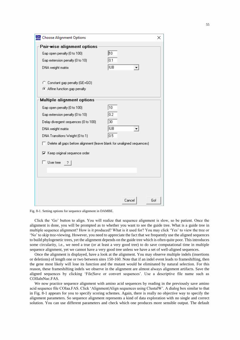
55
Fig. 8-1. Setting options for sequence alignment in DAMBE.
Click the ‘Go’ button to align. You will realize that sequence alignment is slow, so be patient. Once the
alignment is done, you will be prompted as to whether you want to see the guide tree. What is a guide tree in
multiple sequence alignment? How is it produced? What is it used for? You may click ‘Yes’ to view the tree or
‘No’ to skip tree-viewing. However, you need to appreciate the fact that we frequently use the aligned sequences
to build phylogenetic trees, yet the alignment depends on the guide tree which is often quite poor. This introduces
some circularity, i.e., we need a true (or at least a very good tree) to do save computational time in multiple
sequence alignment, yet we cannot have a very good tree unless we have a set of well-aligned sequences.
Once the alignment is displayed, have a look at the alignment. You may observe multiple indels (insertions
or deletions) of length one or two between sites 150-160. Note that if an indel event leads to frameshifting, then
the gene most likely will lose its function and the mutant would be eliminated by natural selection. For this
reason, these frameshifting indels we observe in the alignment are almost always alignment artifacts. Save the
aligned sequences by clicking ‘File|Save or convert sequences’. Use a descriptive file name such as
COIIalnNuc.FAS.
We now practice sequence alignment with amino acid sequences by reading in the previously save amino
acid sequence file COIaa.FAS. Click ‘Alignment|Align sequences using ClustalW’. A dialog box similar to that
in Fig. 8-1 appears for you to specify scoring schemes. Again, there is really no objective way to specify the
alignment parameters. So sequence alignment represents a kind of data exploration with no single and correct
solution. You can use different parameters and check which one produces more sensible output. The default

56
protein weight matrix is BLOSUM. There are several other matrices that you can choose from. All of them try
to weight amino acid pairs according to the empirical substitution frequencies between amino acids. There is a
great deal of information on amino acid substitution matrices on the web in case you are interested. So I will not
provide any details here.
Click the ‘Go’ button to align. Once the alignment is done, you may click ‘Yes’ to view the guide tree or
‘No’ to skip tree-viewing. Save the aligned amino acid sequences to a file named COIIaaAln.FAS.
Align protein-coding nucleotide sequences against aligned amino acid sequences
Recall that the indels of one or two nucleotides in the aligned nucleotide sequences are alignment artifacts
and are consequently undesirable. Here we introduce an approach to eliminate such artifacts by aligning protein-
coding nucleotide sequences against aligned amino acid sequences.
We will use the COII.FAS to illustrate the procedure. Sequences in this file satisfy the minimum requirement
for aligning the nucleotide sequences against aligned amino acid sequences, i.e., there is no embedded stop
codon in the sequences.
Read in the COII.FAS. Click ‘Sequence|Working on amino acid sequence’ to translate the nucleotide
sequences into amino acid sequences. It is important to make sure that the sequences are of high quality and that
no sequence represents a pseudogene with embedded stop codons because such low-quality or pseudogene
sequences invalidate this approach of aligning nucleotide sequences against aligned amino acid sequences. This
is because low-quality or pseudogene sequences have a high chance of having indels of one or two bases, i.e.,
they are real and not alignment artifacts. Press Ctrl-F to search for ‘*’ (without quotes), which stands for
termination signal (i.e., resulting from, e.g., TAA). If there is an embedded ‘*’ in a sequence, then the sequence
is either of low quality or probably from a pseudogene, and should not be used with this function.
Click ‘Alignment|Align sequences using ClustalW’ to align the amino acid sequences. Click
‘Alignment|Align nuc sequences against aligned aa sequences’. When prompted for a file, browse and open the
COII.FAS file. The aligned sequences will be displayed. You will notice that all indels are either in triplets or
multiples of triplets. There is no indel of one or two bases.
A preview of molecular phylogenetics
A molecular phylogenetic tree can be built from a set of alignment sequences. There are four categories of
molecular phylogenetic methods: distance-based, maximum parsimony, maximum likelihood and Bayesian
inference. Here we will use only the distance-based method.
We have already saved to file COIIaln.FAS a set of aligned nucleotide sequences, and to file COIIaaAln.FAS
a set of aligned amino acid sequences. Because third codon position in protein-coding genes often evolve so fast
that substantial substitution saturation would occur between highly diverged taxonomic groups (Xia, et al. 1996;
Xia 1998b), molecular phylogeneticists often believe that amino acid sequences would generate more reliable
trees than nucleotide sequences. Because we have both aligned nucleotide and aligned amino sequences, we are
in a position to check this belief.
Read in the COIIaln.FAS file. Click ‘Phylogenetics|Distance methods|Nucleotide sequences’ and set the
options in the next dialog box (Fig. 8-2). For any distance-based method involving nucleotide sequences, one
needs to specify (1) the genetic distance to be used and (2) the phylogenetic algorithm that uses the distance
matrix to build the tree to facilitate the reproduction of the result. We will use Lake’s paralinear distance or
Lake94 (Lake 1994) and the FastME algorithm (Desper and Gascuel 2002, 2004).
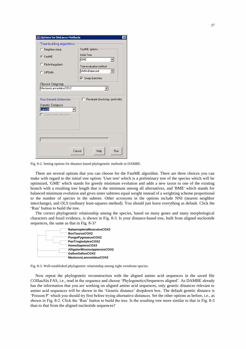
57
Fig. 8-2. Setting options for distance-based phylogenetic methods in DAMBE.
There are several options that you can choose for the FastME algorithm. There are three choices you can
make with regard to the initial tree option: 'User tree' which is a preliminary tree of the species which will be
optimized, 'GME' which stands for greedy minimum evolution and adds a new taxon to one of the existing
branch with a resulting tree length that is the minimum among all alternatives, and 'BME' which stands for
balanced minimum evolution and gives sister subtrees equal weight instead of a weighting scheme proportional
to the number of species in the subtree. Other acronyms in the options include NNI (nearest neighbor
interchange), and OLS (ordinary least-squares method). You should just leave everything as default. Click the
‘Run’ button to build the tree.
The correct phylogenetic relationship among the species, based on many genes and many morphological
characters and fossil evidence, is shown in Fig. 8-3. Is your distance-based tree, built from aligned nucleotide
sequences, the same as that in Fig. 8-3?
MasturusLanceolatusCOX2
GallusGallusCOX2
AlligatorMississippiensisCOX2
HomoSapiensCOX2
PanTroglodytesCOX2
PongoPygmaeusCOX2
BosTaurusCOX2
BalaenopteraMusculusCOX2
Fig. 8-3. Well-established phylogenetic relationship among eight vertebrate species.
Now repeat the phylogenetic reconstruction with the aligned amino acid sequences in the saved file
COIIaaAln.FAS, i.e., read in the sequence and choose ‘Phylogenetics|Sequences aligned’. As DAMBE already
has the information that you are working on aligned amino acid sequences, only genetic distances relevant to
amino acid sequences will be shown in the ‘Genetic distance’ dropdown box. The default genetic distance is
‘Poisson P’ which you should try first before trying alternative distances. Set the other options as before, i.e., as
shown in Fig. 8-2. Click the ‘Run’ button to build the tree. Is the resulting tree more similar to that in Fig. 8-3
than to that from the aligned nucleotide sequences?

58
More questions
1. With the constant gap penalty, how much memory would be needed for the scoring matrix in aligning two
sequences with lengths of M and N nt long, respectively, if we use only integers in the scoring scheme and
four bytes are used to hold an integer? (The memory requirement would be at least three times more if we
distinguish between gap open and gap extension.)
2. Complete the following scoring matrix and backtrack matrix, with 2, and -1 being the match and mismatch
scores, respectively, and -3 being constant gap penalty. Obtain the sequence alignment and the alignment
score. Identify cell with two possible arrows indicating two alternative optimal alignments. There may be
several such cells, but you need only to find one along the backtrack path.
41-1-3-8-13-18G
47420-5-10-15A
-1253-2-7-12C
-6-30361-4-9T
-11-8-5-21-6A
-16-13-10-7-4-3A
-21-18-15-12-9-6-30
GACTTAA
3. What is the advantage of aligning protein-coding nucleotide sequences against aligned amino acid sequences?
4. What is the minimum requirement for aligning protein-coding nucleotide sequences against aligned amino
acid sequences?
5. What are the main differences in dynamic programming between local and global sequence alignment?
6. Is Clustal alignment program based on global alignment algorithms whereas BLAST and FASTA algorithms
are based on local similarity searches?
7. Given the following two alignments labeled (1) and (2), provide the simplest possible scoring scheme that
will give Alignment 1 a higher alignment score than Alignment 2 and give the alignment score for Alignment
1 and Alignment 2 according to the scoring scheme.
(1) (2)
ACG--T AC-G-T
ACGGCT ACGGCT
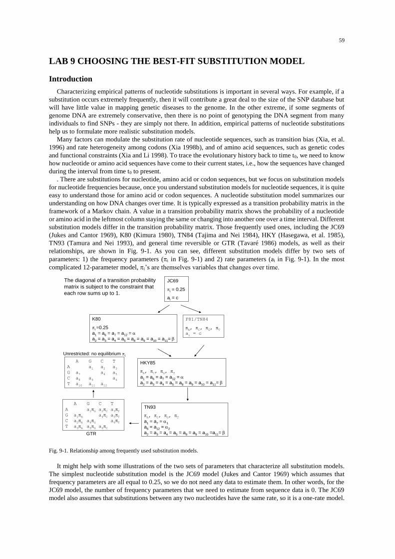
59
LAB 9 CHOOSING THE BEST-FIT SUBSTITUTION MODEL
Introduction
Characterizing empirical patterns of nucleotide substitutions is important in several ways. For example, if a
substitution occurs extremely frequently, then it will contribute a great deal to the size of the SNP database but
will have little value in mapping genetic diseases to the genome. In the other extreme, if some segments of
genome DNA are extremely conservative, then there is no point of genotyping the DNA segment from many
individuals to find SNPs - they are simply not there. In addition, empirical patterns of nucleotide substitutions
help us to formulate more realistic substitution models.
Many factors can modulate the substitution rate of nucleotide sequences, such as transition bias (Xia, et al.
1996) and rate heterogeneity among codons (Xia 1998b), and of amino acid sequences, such as genetic codes
and functional constraints (Xia and Li 1998). To trace the evolutionary history back to time t0, we need to know
how nucleotide or amino acid sequences have come to their current states, i.e., how the sequences have changed
during the interval from time t0 to present.
. There are substitutions for nucleotide, amino acid or codon sequences, but we focus on substitution models
for nucleotide frequencies because, once you understand substitution models for nucleotide sequences, it is quite
easy to understand those for amino acid or codon sequences. A nucleotide substitution model summarizes our
understanding on how DNA changes over time. It is typically expressed as a transition probability matrix in the
framework of a Markov chain. A value in a transition probability matrix shows the probability of a nucleotide
or amino acid in the leftmost column staying the same or changing into another one over a time interval. Different
substitution models differ in the transition probability matrix. Those frequently used ones, including the JC69
(Jukes and Cantor 1969), K80 (Kimura 1980), TN84 (Tajima and Nei 1984), HKY (Hasegawa, et al. 1985),
TN93 (Tamura and Nei 1993), and general time reversible or GTR (Tavaré 1986) models, as well as their
relationships, are shown in Fig. 9-1. As you can see, different substitution models differ by two sets of
parameters: 1) the frequency parameters (i in Fig. 9-1) and 2) rate parameters (ai in Fig. 9-1). In the most
complicated 12-parameter model, i’s are themselves variables that changes over time.
A G C T
A a1
a2
a3
G a7
a4
a5
C a8
a9
a6
T a10
a11
a12
A G C T
A a1Ga2Ca3T
G a1A
a4Ca5T
C a2A
a4G
a6T
T a3A
a5Ga6C
The diagonal of a transition probability
matrix is subject to the constraint that
each row sums up to 1.
JC69
i = 0.25
ai = c
F81/TN84
A,
C,
G,
T
ai= c
K80
i =0.25
a1 = a6 = a7 = a12 =
a2 = a3 = a4 = a5 = a8 = a9 = a10 = a11=
HKY85
A,
C,
G,
T
a1 = a6 = a7 = a12 =
a2 = a3 = a4 = a5 = a8 = a9 = a10 = a11=
TN93
A,
C,
G,
T
a1 = a7 = 1
a6 = a12 = 2
a2 = a3 = a4 = a5 = a8 = a9 = a10 =a11= GTR
Unrestricted: no equilibrium i
Fig. 9-1. Relationship among frequently used substitution models.
It might help with some illustrations of the two sets of parameters that characterize all substitution models.
The simplest nucleotide substitution model is the JC69 model (Jukes and Cantor 1969) which assumes that
frequency parameters are all equal to 0.25, so we do not need any data to estimate them. In other words, for the
JC69 model, the number of frequency parameters that we need to estimate from sequence data is 0. The JC69
model also assumes that substitutions between any two nucleotides have the same rate, so it is a one-rate model.

60
If you have sequences whose frequencies differ substantially from 0.25, or if transitions occur more frequently
than transversions, then the assumptions of JC69 are violated and you should not use JC69 for your sequences.
If your sequences do have equal nucleotide frequencies, but transitions and transversions occur at different
rate (typically transitions occur much more frequently than transversions), then you should use the K80 model
(Kimura 1980) which let transitions have one rate and transversions another rate. So K80 model is a two-rate
model in contrast to JC69 which is a one-rate model. However, both JC69 and K80 assume equal nucleotide
frequencies. To be more descriptive, you may refer to JC69 as a one-rate, equal-frequency model, and K80 as a
two-rate, equal-frequency model. If transition rate and transversion rate are in fact the same, then K80 is reduced
to JC69. Thus, JC69 is a special case of K80. When one model is a special case of another more general model,
we say the two models are nested.
Here is a concrete example of nested models. Suppose Model 1 is Y = aX, and Model 2 is Y = aXb. If b is in
fact equal to 1, then Model 2 is reduced to Model 1. The two models are nested with Model 1being a special
case of Model 2. We will learn that, for nested models, we can use likelihood ratio tests for model selection.
On the other hand if different nucleotides do change into each other with the same rate, but sequences differ
in frequencies, then you can use the F81/TN84 model (Tajima and Nei 1984) which is also a one-rate model but
differs from the JC69 model in that the former allow nucleotide frequencies to be different. So you may refer to
F81/TN84 as a one-rate, different-frequency model. Thus, JC69 and F81/TN84 are also nested because JC69 is
a special case of F81/TN84. If the nucleotide frequencies are in fact equal, then F81/TN84 is reduced to JC69.
Note that, in F81/TN84, we need to estimate THREE nucleotide frequencies from the nucleotide sequence data.
The reason that it is three instead of four is that, once we know three frequencies (e.g., PA, PC, PG), the 4th (e.g.,
PT) is determined (i.e., not free) because PT = 1 - PA - PC - PG.
If your sequences not only have different nucleotide frequencies, but the transition rate also differs from the
transversion rate, then you cannot use JC69, K80 or F81/TN84. Instead, you should use HKY85 (Hasegawa, et
al. 1985) or F84 (Felsenstein 2004), the two being equally general). These two are two-rate, different-frequency
models. If the two rates are in fact equal, then HKY85 and F84 are reduced to F81/TN84. If the frequencies are
in fact equal, then HKY85 and F84 are reduced to K80.
If your sequences not only have different nucleotide frequencies and different the transition and transversion
rates, but the two transition rates (i.e., A G and C T) are also different, then you should not use any of
those models mentioned above because now you have three rates: two for the two types of transitions and one
for all transversions. Instead, you should use TN93 (Tamura and Nei 1993) which allows the nucleotide
frequencies to be different as well as the three rates to be different. So TN93 is a three-rate, different-frequency
model. If the two transitions in fact have the same rate, then TN93 is reduced to HKY85.
If your sequences not only have different frequencies, but all nucleotides change each other with different
rates, then you should use GTR (for General Time-Reversible) which have six rates (Tavaré 1986).
All models that we have mentioned so far are time-reversible models. Time-reversible means that a nucleotide
(say A) change into any other nucleotide is balanced by other nucleotide changing to A. This means that you
can have all kinds of changes, but the frequencies will stay the same. If the ancestral sequence have frequencies
for A, C, G, T being 0.1, 0.4, 0.4, 0.1, then all descendent sequences are also expected to have the same
frequencies.
There are cases in which time-reversibility is violated. For example, if there is a high tendency for
spontaneous mutation of C to U (or methylated C to T), then C will become fewer and fewer and T become more
and more in descendent sequences. If C to T mutations occur frequently in the vertebrate lineages, but rarely in
invertebrate lineages, then you may have frequencies for A, C, G, T being 0.1, 0.4, 0.4, 0.1 in some lineages but
0.4, 0.1, 0.1, 0.4 in others. In this case, you should not use time-reversible models but instead should use the
Unrestricted model (which in practice is almost never used in teaching or research because it has too many
parameters to be practical).
With the conceptual framework above, it is not difficult to understand substitution models for amino acid and
codon sequences. Now we know that all substitution models are characterized by the frequency parameters and
rate parameters. For amino acid sequences, there are 19 frequency parameters to estimate from the data, but the
rate parameters are a bit complex. We know that some amino acid replacements occurs very frequently, e.g.,
between Gly and Ala, but others occur rarely, e.g., between Gly and Tyr. So different amino acid substitutions
should have different rates, but there would be 20*19/2 rates assuming time-reversibility which are too many to
estimate for any real amino acid sequence alignment. As a sub-optimal alternative, we typically use an empirical
substitution matrix (e.g., a Blosum or Dayhoff matrix) as an approximation to the rates.
For codon sequences, we typically ignore the termination codons because any substitution from a sense codon
to a termination codon is typically highly deleterious with an extremely low fixation probability. There are 61
61
sense codons for the standard genetic code, so we have 60 frequency parameters to estimate from the data. We
also have 61*60/2 rate parameters which are simply monstrous. Instead, a typical codon-based substitution
model will only estimate the transition and transversion rates and the synonymous and nonsynonymous rates. In
other words, GGA GGG and GGC GGT will have the same rate because both substitutions involve a
transition and both are synonymous (they both code Gly). However, GGA GGG and GGA GGT will have
different rates because the former involves a transition and the latter a transversion. Also, GGG GGA and
GGG GAG will have different rates because, although both involve a G A transition, the former is
synonymous and the latter is nonsynonymous.
Substitution models are the foundation of the maximum likelihood method and the distance-based method in
molecular phylogenetics. A genetic distance in molecular phylogenetics is often prefixed with the substitution
model from which it is derived, e.g., JC69 distance is derived from the JC69 substitution model (Jukes and
Cantor 1969). The maximum likelihood method for phylogenetic analysis (Felsenstein 2004, 2014), which has
increased its popularity in recent years with the increasingly faster computers, assumes a substitution model for
computing the likelihood of the tree. Recently, scientists have tried to reconstruct ancestral protein-coding
sequence based on substitution models, synthesizing the reconstructed protein, and explore its function and
evolution (Chang, Jonsson, et al. 2002; Chang, Kazmi, et al. 2002; Ugalde, et al. 2004). If the substitution model
is good, then the likelihood of the reconstruction being correct is increased. Given that substitution models are
used wide in molecular phylogenetics, we need to develop an appreciation of the differences among different
genetic models and to understand how to choose one substitution model over others in practical applications.
In this laboratory, we will first take a guided empirical approach to understanding the various nucleotide
substitution models implemented in DAMBE. In short, we will take a set of aligned sequences and characterize
nucleotide frequencies and substitution patterns, which are then used as the basis for choosing substitution
models.
Characterizing nucleotide frequencies may seem straightforward – you only need to count the number of A,
C, G and T, designated NA, NC, NG and NT, in the sequences, and obtain the estimated frequencies by NA/N,
NC/N, NG/N and NT/N, where N = NA + NC + NG + NT. However, for a set of aligned sequences, there are often
conserved sites and variable sites. For example, 18S rRNA sequences have conserved domains and variable
domains, with the nucleotide frequencies in the former differing from those in the latter. Because substitutions
occur frequently at the variable domains but rarely at the conservative domains, it is the nucleotide frequencies
at the variable domains that are the most relevant for substitution models (Xia, et al. 2003). However, the variable
domains also experience insertions/deletions (indels) and a site containing indels are often deleted from analysis,
resulting in nucleotide frequencies at the conserved domains dominating in estimating overall nucleotide
frequencies. This can lead to bias in phylogenetic estimation (Xia, et al. 2003).
Characterizing an empirical substitution pattern also seems straightforward – you compare two sequences
and count the differences. For example, if one sequence has A at site 11, and the other sequence has G at the
same site, then we record an AG or GA transition if the tree is rooted or just an AG transition if the tree
is not rooted so we do not know the direction of change. However, empirical substitution patterns based on all
pairwise comparisons can be misleading. For illustration, suppose we have five sequences, with the first four
sequences very similar to each other, but the 5th sequence is very different from the rest. If we perform all
possible pair-wise comparisons, then nearly all differences are between the 5th sequence and the other four
sequences. In other words, any difference between the 5th sequence and the other four sequences is counted four
times. To alleviate this problem, we would build a phylogenetic tree, reconstruct ancestral sequences and
perform pairwise comparisons between neighboring nodes along the tree. Thus, for the tree in Fig. 9-2, there are
only seven pairwise comparisons in contrast to 10 possible pairwise comparisons for five OTUs. If OTU5
represents the odd sequence, then its unique differences will only contribute to the comparison between IN8 and
OTU5 (Fig. 9-2).
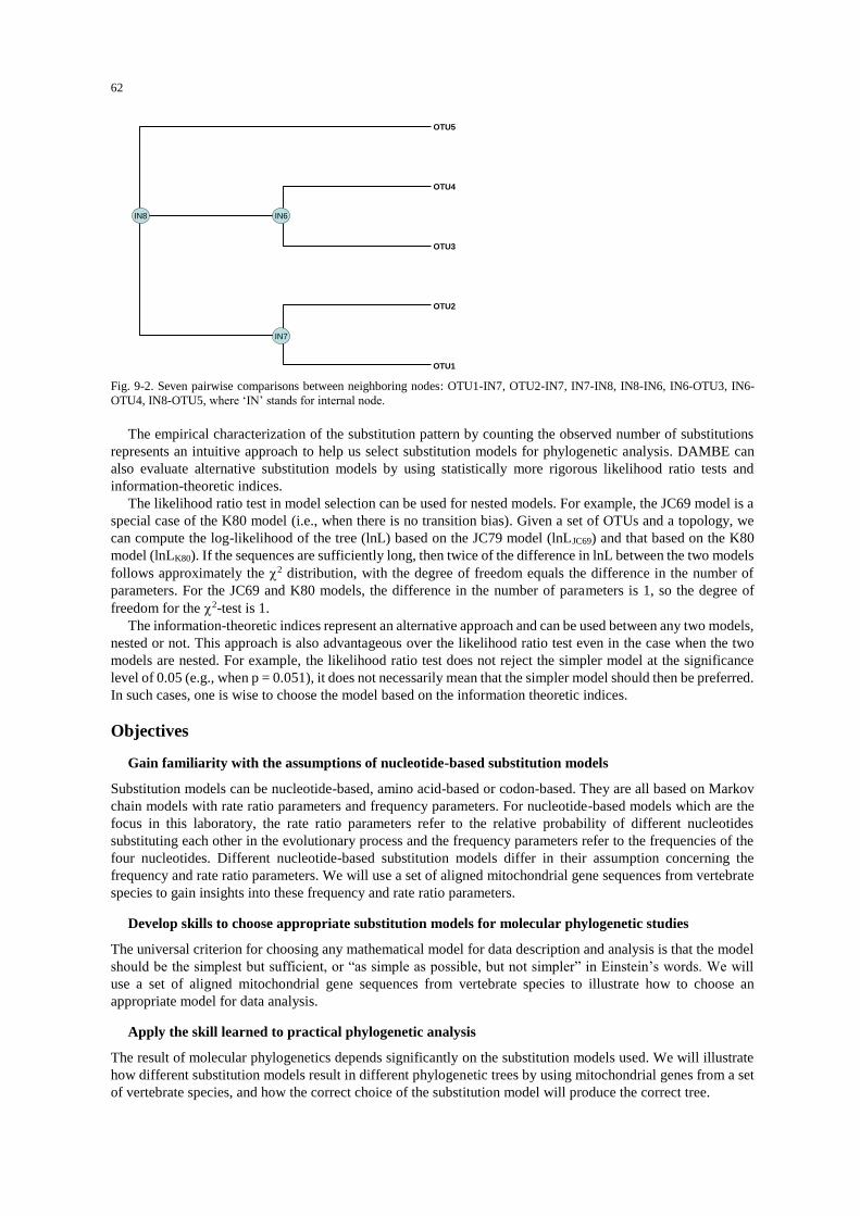
62
OTU1
OTU2
OTU3
OTU4
OTU5
IN6IN8
IN7
Fig. 9-2. Seven pairwise comparisons between neighboring nodes: OTU1-IN7, OTU2-IN7, IN7-IN8, IN8-IN6, IN6-OTU3, IN6-
OTU4, IN8-OTU5, where ‘IN’ stands for internal node.
The empirical characterization of the substitution pattern by counting the observed number of substitutions
represents an intuitive approach to help us select substitution models for phylogenetic analysis. DAMBE can
also evaluate alternative substitution models by using statistically more rigorous likelihood ratio tests and
information-theoretic indices.
The likelihood ratio test in model selection can be used for nested models. For example, the JC69 model is a
special case of the K80 model (i.e., when there is no transition bias). Given a set of OTUs and a topology, we
can compute the log-likelihood of the tree (lnL) based on the JC79 model (lnLJC69) and that based on the K80
model (lnLK80). If the sequences are sufficiently long, then twice of the difference in lnL between the two models
follows approximately the 2 distribution, with the degree of freedom equals the difference in the number of
parameters. For the JC69 and K80 models, the difference in the number of parameters is 1, so the degree of
freedom for the 2-test is 1.
The information-theoretic indices represent an alternative approach and can be used between any two models,
nested or not. This approach is also advantageous over the likelihood ratio test even in the case when the two
models are nested. For example, the likelihood ratio test does not reject the simpler model at the significance
level of 0.05 (e.g., when p = 0.051), it does not necessarily mean that the simpler model should then be preferred.
In such cases, one is wise to choose the model based on the information theoretic indices.
Objectives
Gain familiarity with the assumptions of nucleotide-based substitution models
Substitution models can be nucleotide-based, amino acid-based or codon-based. They are all based on Markov
chain models with rate ratio parameters and frequency parameters. For nucleotide-based models which are the
focus in this laboratory, the rate ratio parameters refer to the relative probability of different nucleotides
substituting each other in the evolutionary process and the frequency parameters refer to the frequencies of the
four nucleotides. Different nucleotide-based substitution models differ in their assumption concerning the
frequency and rate ratio parameters. We will use a set of aligned mitochondrial gene sequences from vertebrate
species to gain insights into these frequency and rate ratio parameters.
Develop skills to choose appropriate substitution models for molecular phylogenetic studies
The universal criterion for choosing any mathematical model for data description and analysis is that the model
should be the simplest but sufficient, or “as simple as possible, but not simpler” in Einstein’s words. We will
use a set of aligned mitochondrial gene sequences from vertebrate species to illustrate how to choose an
appropriate model for data analysis.
Apply the skill learned to practical phylogenetic analysis
The result of molecular phylogenetics depends significantly on the substitution models used. We will illustrate
how different substitution models result in different phylogenetic trees by using mitochondrial genes from a set
of vertebrate species, and how the correct choice of the substitution model will produce the correct tree.
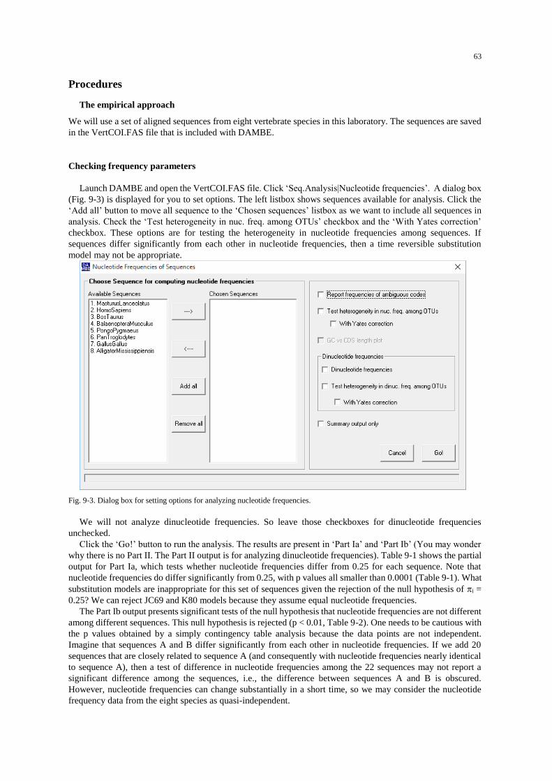
63
Procedures
The empirical approach
We will use a set of aligned sequences from eight vertebrate species in this laboratory. The sequences are saved
in the VertCOI.FAS file that is included with DAMBE.
Checking frequency parameters
Launch DAMBE and open the VertCOI.FAS file. Click ‘Seq.Analysis|Nucleotide frequencies’. A dialog box
(Fig. 9-3) is displayed for you to set options. The left listbox shows sequences available for analysis. Click the
‘Add all’ button to move all sequence to the ‘Chosen sequences’ listbox as we want to include all sequences in
analysis. Check the ‘Test heterogeneity in nuc. freq. among OTUs’ checkbox and the ‘With Yates correction’
checkbox. These options are for testing the heterogeneity in nucleotide frequencies among sequences. If
sequences differ significantly from each other in nucleotide frequencies, then a time reversible substitution
model may not be appropriate.
Fig. 9-3. Dialog box for setting options for analyzing nucleotide frequencies.
We will not analyze dinucleotide frequencies. So leave those checkboxes for dinucleotide frequencies
unchecked.
Click the ‘Go!’ button to run the analysis. The results are present in ‘Part Ia’ and ‘Part Ib’ (You may wonder
why there is no Part II. The Part II output is for analyzing dinucleotide frequencies). Table 9-1 shows the partial
output for Part Ia, which tests whether nucleotide frequencies differ from 0.25 for each sequence. Note that
nucleotide frequencies do differ significantly from 0.25, with p values all smaller than 0.0001 (Table 9-1). What
substitution models are inappropriate for this set of sequences given the rejection of the null hypothesis of i =
0.25? We can reject JC69 and K80 models because they assume equal nucleotide frequencies.
The Part Ib output presents significant tests of the null hypothesis that nucleotide frequencies are not different
among different sequences. This null hypothesis is rejected (p < 0.01, Table 9-2). One needs to be cautious with
the p values obtained by a simply contingency table analysis because the data points are not independent.
Imagine that sequences A and B differ significantly from each other in nucleotide frequencies. If we add 20
sequences that are closely related to sequence A (and consequently with nucleotide frequencies nearly identical
to sequence A), then a test of difference in nucleotide frequencies among the 22 sequences may not report a
significant difference among the sequences, i.e., the difference between sequences A and B is obscured.
However, nucleotide frequencies can change substantially in a short time, so we may consider the nucleotide
frequency data from the eight species as quasi-independent.
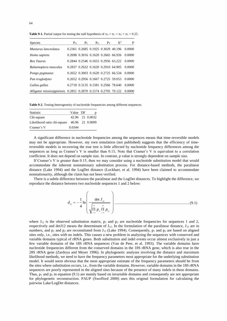
64
Table 9-1. Partial output for testing the null hypothesis of A = C = G = T = 0.25.
Species PA PC PG PT X2 P
Masturus lanceolatus 0.2361 0.2685 0.1925 0.3029 40.196 0.0000
Homo sapiens 0.2698 0.3016 0.1620 0.2665 66.926 0.0000
Bos Taurus 0.2844 0.2546 0.1653 0.2956 63.222 0.0000
Balaenoptera musculus 0.2837 0.2632 0.1620 0.2910 64.905 0.0000
Pongo pygmaeus 0.2652 0.3003 0.1620 0.2725 66.534 0.0000
Pan troglodytes 0.2652 0.2956 0.1667 0.2725 59.053 0.0000
Gallus gallus 0.2718 0.3135 0.1581 0.2566 78.640 0.0000
Alligator mississippiensis 0.2851 0.2870 0.1574 0.2705 70.122 0.0000
Table 9-2. Testing heterogeneity of nucleotide frequencies among different sequences.
Statistic Value DF p
Chi-square 42.96 21 0.0032
Likelihood ratio chi-square 46.96 21 0.0009
Cramer’s V 0.0344
A significant difference in nucleotide frequencies among the sequences means that time-reversible models
may not be appropriate. However, my own simulation (not published) suggests that the efficiency of time-
reversible models in recovering the true tree is little affected by nucleotide frequency differences among the
sequences as long as Cramer’s V is smaller than 0.15. Note that Cramer’s V is equivalent to a correlation
coefficient. It does not depend on sample size. In contrast, p value is strongly dependent on sample size.
If Cramer’s V is greater than 0.15, then we may consider using a nucleotide substitution model that would
accommodate the inherent nonstationary substitution process. For distance-based methods, the paralinear
distance (Lake 1994) and the LogDet distance (Lockhart, et al. 1994) have been claimed to accommodate
nonstationarity, although the claim has not been verified.
There is a subtle difference between the paralinear and the LogDet distances. To highlight the difference, we
reproduce the distance between two nucleotide sequences 1 and 2 below:
12
124 4
1 21 1
det1ln
4i i
i i
Jd
p p
.............................................................................. (9.1)
where J12 is the observed substitution matrix, p1 and p2 are nucleotide frequencies for sequences 1 and 2,
respectively and detJ12 means the determinant of J12. In the formulation of the paralinear distance, J12 are in
numbers, and p1 and p2 are reconstituted from J12 (Lake 1994). Consequently, p1 and p2 are based on aligned
sites only, i.e., sites with no indels. This causes a new problem in analyzing the sequences with conserved and
variable domains typical of rRNA genes. Both substitution and indel events occur almost exclusively in just a
few variable domains of the 18S rRNA sequences (Van de Peer, et al. 1993). The variable domains have
nucleotide frequencies different from the conserved domains in the 18S rRNA gene, which is also true in the
28S rRNA gene (Zardoya and Meyer 1996). In phylogenetic analyses involving the distance and maximum
likelihood methods, we need to have the frequency parameters most appropriate for the underlying substitution
model. It would seem obvious that the most appropriate estimate of the frequency parameters should be from
the sites where substitution occurs, i.e., from the variable domains. However, variable domains in the 18S rRNA
sequences are poorly represented in the aligned sites because of the presence of many indels in these domains.
Thus, p1 and p2 in equation (9.1) are mainly based on invariable domains and consequently are not appropriate
for phylogenetic reconstruction. PAUP (Swofford 2000) uses this original formulation for calculating the
pairwise Lake/LogDet distances.

65
An alternative is to use the LogDet distance (Lockhart, et al. 1994) which defines J12 as a substitution matrix
in proportions summing up to 1, and p1 and p2 as vectors of proportions summing up to 1. This permits the
computation of empirical frequencies from all sites, including sites containing indels. Both DAMBE and the
DNADIST program in PHYLIP (Felsenstein 2014) use all sites in computing p1 and p2. This approach allow
sites in the variable domains of the 18S rRNA sequences to be better represented in computing nucleotide
frequencies, and is the approach that we have taken in analyzing the 18S rRNA sequences.
Checking rate parameters
While the sequences are still in DAMBE, click ‘Seq. Analysis|Nucleotide substitution pattern|Detailed output’.
The dialog shows two listboxes, with the left showing the sequences available for analysis and the right showing
sequences that you have chosen to do the analysis. Click the ‘Add all’ button to move all sequences to the right
(Fig. 9-4), and click the ‘Go!’ button. DAMBE will characterize nucleotide substitution patterns from all
pairwise comparisons.
Fig. 9-4. Dialog box for characterizing nucleotide substitution pattern.
Once DAMBE finishes documenting the substitution patterns, you will be asked if you want to see the number
of transitions and transversions plotted against the K80 or F84 distances. This is for visualizing substitution
saturation which would erase historical information written in nucleotide sequences. For pairs of highly diverged
taxa experiencing high substitution saturation, transversions will outnumber transitions. If sequences evolve
according to the JC69 or K80 models, transversions will be twice as many as transitions for pairs of sequences
experiencing full substitution saturation. Such sequences would be of little use for reconstructing phylogenetic
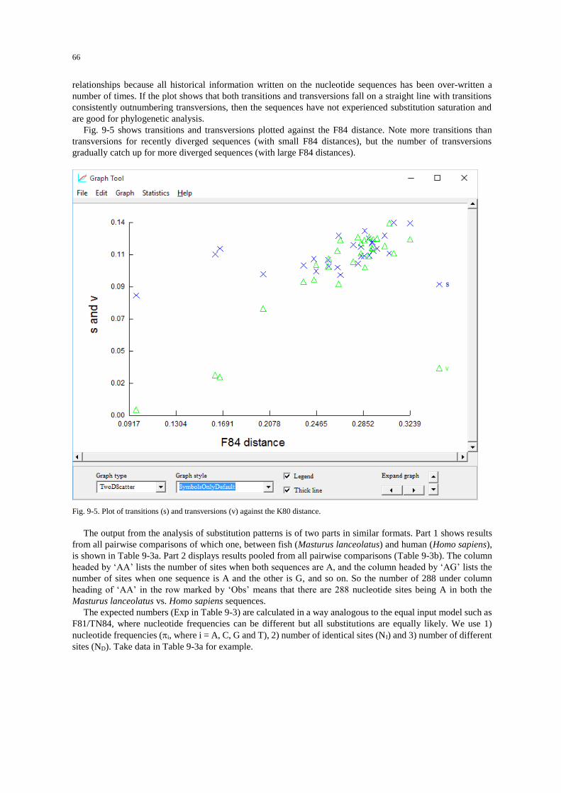
66
relationships because all historical information written on the nucleotide sequences has been over-written a
number of times. If the plot shows that both transitions and transversions fall on a straight line with transitions
consistently outnumbering transversions, then the sequences have not experienced substitution saturation and
are good for phylogenetic analysis.
Fig. 9-5 shows transitions and transversions plotted against the F84 distance. Note more transitions than
transversions for recently diverged sequences (with small F84 distances), but the number of transversions
gradually catch up for more diverged sequences (with large F84 distances).
Fig. 9-5. Plot of transitions (s) and transversions (v) against the K80 distance.
The output from the analysis of substitution patterns is of two parts in similar formats. Part 1 shows results
from all pairwise comparisons of which one, between fish (Masturus lanceolatus) and human (Homo sapiens),
is shown in Table 9-3a. Part 2 displays results pooled from all pairwise comparisons (Table 9-3b). The column
headed by ‘AA’ lists the number of sites when both sequences are A, and the column headed by ‘AG’ lists the
number of sites when one sequence is A and the other is G, and so on. So the number of 288 under column
heading of ‘AA’ in the row marked by ‘Obs’ means that there are 288 nucleotide sites being A in both the
Masturus lanceolatus vs. Homo sapiens sequences.
The expected numbers (Exp in Table 9-3) are calculated in a way analogous to the equal input model such as
F81/TN84, where nucleotide frequencies can be different but all substitutions are equally likely. We use 1)
nucleotide frequencies (i, where i = A, C, G and T), 2) number of identical sites (NI) and 3) number of different
sites (ND). Take data in Table 9-3a for example.
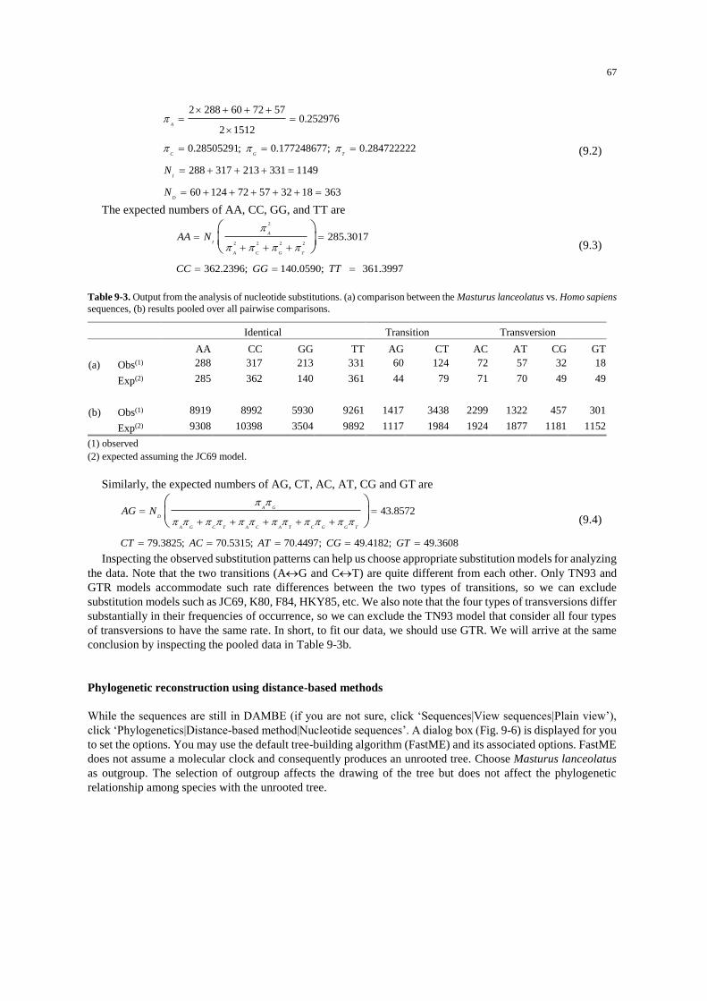
67
2 288 60 72 570.252976
2 1512
0.28505291; 0.177248677; 0.284722222
288 317 213 331 1149
60 124 72 57 32 18 363
A
C G T
I
D
N
N
(9.2)
The expected numbers of AA, CC, GG, and TT are
2
2 2 2 2285.3017
362.2396; 140.0590; 361.3997
A
I
A C G T
AA N
CC GG TT
(9.3)
Table 9-3. Output from the analysis of nucleotide substitutions. (a) comparison between the Masturus lanceolatus vs. Homo sapiens
sequences, (b) results pooled over all pairwise comparisons.
Identical Transition Transversion
AA CC GG TT AG CT AC AT CG GT
(a) Obs(1) 288 317 213 331 60 124 72 57 32 18
Exp(2) 285 362 140 361 44 79 71 70 49 49
(b) Obs(1) 8919 8992 5930 9261 1417 3438 2299 1322 457 301
Exp(2) 9308 10398 3504 9892 1117 1984 1924 1877 1181 1152
(1) observed
(2) expected assuming the JC69 model.
Similarly, the expected numbers of AG, CT, AC, AT, CG and GT are
43.8572
79.3825; 70.5315; 70.4497; 49.4182; 49.3608
A G
D
A G C T A C A T C G G T
AG N
CT AC AT CG GT
(9.4)
Inspecting the observed substitution patterns can help us choose appropriate substitution models for analyzing
the data. Note that the two transitions (AG and CT) are quite different from each other. Only TN93 and
GTR models accommodate such rate differences between the two types of transitions, so we can exclude
substitution models such as JC69, K80, F84, HKY85, etc. We also note that the four types of transversions differ
substantially in their frequencies of occurrence, so we can exclude the TN93 model that consider all four types
of transversions to have the same rate. In short, to fit our data, we should use GTR. We will arrive at the same
conclusion by inspecting the pooled data in Table 9-3b.
Phylogenetic reconstruction using distance-based methods
While the sequences are still in DAMBE (if you are not sure, click ‘Sequences|View sequences|Plain view’),
click ‘Phylogenetics|Distance-based method|Nucleotide sequences’. A dialog box (Fig. 9-6) is displayed for you
to set the options. You may use the default tree-building algorithm (FastME) and its associated options. FastME
does not assume a molecular clock and consequently produces an unrooted tree. Choose Masturus lanceolatus
as outgroup. The selection of outgroup affects the drawing of the tree but does not affect the phylogenetic
relationship among species with the unrooted tree.

68
Fig. 9-6. Setting options for distance-based methods in molecular phylogenetics.
For evolutionary distance, we will choose GTR because it treats allow all six types of substitutions to have
different rates. Click ‘Run’ to generate the tree (Fig. 9-7) which has internal nodes numbered for later use. You
should learn two more tricks. One is to copy the tree to programs such as PowerPoint for presentation and
publication, and the other is to save the tree for future phylogenetic analysis.
PongoPygmaeus
PanTroglodytes
HomoSapiens
BalaenopteraMusculus
BosTaurus
AlligatorMississippiensis
GallusGallus
MasturusLanceolatus
11
9 14
13
1012
Fig. 9-7. The tree panel in DAMBE.
You can copy and paste the tree to PowerPoint slides or any other graphic programs including EXCEL and
WORD, either in fixed-resolution bitmapped format or in high-resolution Windows metafile format. Appendix
1 summarizes the copying and pasting of trees between DAMBE and PowerPoint.
To save a tree for future viewing or for use with other phylogenetic functions, click ‘File|Save tree for future
viewing’. Give a file name, and the tree will be saved in text format with the file extension of ‘.dnd’ (for
dendrogram). Save the tree that is constructed with the correct substitution model to VertCOI.dnd.
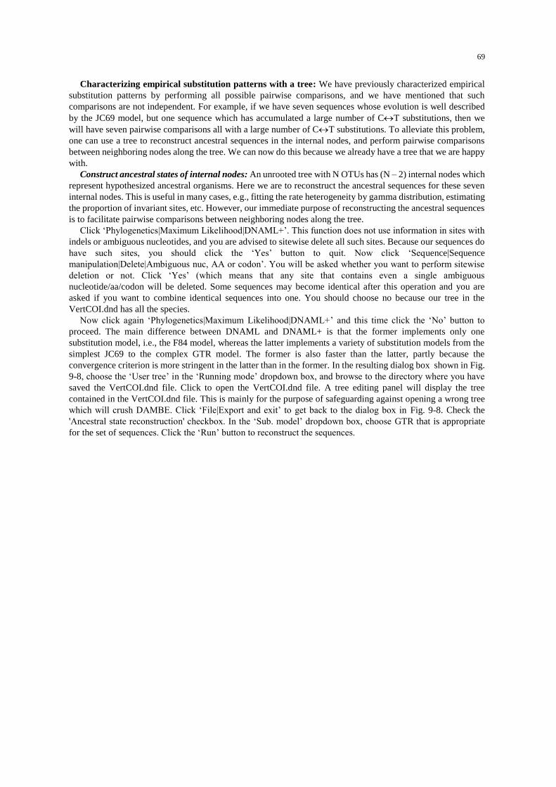
69
Characterizing empirical substitution patterns with a tree: We have previously characterized empirical
substitution patterns by performing all possible pairwise comparisons, and we have mentioned that such
comparisons are not independent. For example, if we have seven sequences whose evolution is well described
by the JC69 model, but one sequence which has accumulated a large number of CT substitutions, then we
will have seven pairwise comparisons all with a large number of CT substitutions. To alleviate this problem,
one can use a tree to reconstruct ancestral sequences in the internal nodes, and perform pairwise comparisons
between neighboring nodes along the tree. We can now do this because we already have a tree that we are happy
with.
Construct ancestral states of internal nodes: An unrooted tree with N OTUs has (N – 2) internal nodes which
represent hypothesized ancestral organisms. Here we are to reconstruct the ancestral sequences for these seven
internal nodes. This is useful in many cases, e.g., fitting the rate heterogeneity by gamma distribution, estimating
the proportion of invariant sites, etc. However, our immediate purpose of reconstructing the ancestral sequences
is to facilitate pairwise comparisons between neighboring nodes along the tree.
Click ‘Phylogenetics|Maximum Likelihood|DNAML+’. This function does not use information in sites with
indels or ambiguous nucleotides, and you are advised to sitewise delete all such sites. Because our sequences do
have such sites, you should click the ‘Yes’ button to quit. Now click ‘Sequence|Sequence
manipulation|Delete|Ambiguous nuc, AA or codon’. You will be asked whether you want to perform sitewise
deletion or not. Click ‘Yes’ (which means that any site that contains even a single ambiguous
nucleotide/aa/codon will be deleted. Some sequences may become identical after this operation and you are
asked if you want to combine identical sequences into one. You should choose no because our tree in the
VertCOI.dnd has all the species.
Now click again ‘Phylogenetics|Maximum Likelihood|DNAML+’ and this time click the ‘No’ button to
proceed. The main difference between DNAML and DNAML+ is that the former implements only one
substitution model, i.e., the F84 model, whereas the latter implements a variety of substitution models from the
simplest JC69 to the complex GTR model. The former is also faster than the latter, partly because the
convergence criterion is more stringent in the latter than in the former. In the resulting dialog box shown in Fig.
9-8, choose the ‘User tree’ in the ‘Running mode’ dropdown box, and browse to the directory where you have
saved the VertCOI.dnd file. Click to open the VertCOI.dnd file. A tree editing panel will display the tree
contained in the VertCOI.dnd file. This is mainly for the purpose of safeguarding against opening a wrong tree
which will crush DAMBE. Click ‘File|Export and exit’ to get back to the dialog box in Fig. 9-8. Check the
'Ancestral state reconstruction' checkbox. In the ‘Sub. model’ dropdown box, choose GTR that is appropriate
for the set of sequences. Click the ‘Run’ button to reconstruct the sequences.
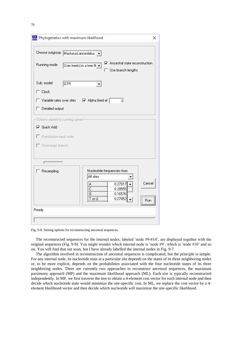
70
Fig. 9-8. Setting options for reconstructing ancestral sequences.
The reconstructed sequences for the internal nodes, labeled ‘node #9-#14’, are displayed together with the
original sequences (Fig. 9-9). You might wonder which internal node is ‘node #9’, which is ‘node #10’ and so
on. You will find that out soon, but I have already labelled the internal nodes in Fig. 9-7.
The algorithm involved in reconstruction of ancestral sequences is complicated, but the principle is simple.
For any internal node, its nucleotide state at a particular site depends on the states of its three neighboring nodes
or, to be more explicit, depends on the probabilities associated with the four nucleotide states of its three
neighboring nodes. There are currently two approaches to reconstruct ancestral sequences, the maximum
parsimony approach (MP) and the maximum likelihood approach (ML). Each site is typically reconstructed
independently. In MP, we first traverse the tree to obtain a 4-element cost vector for each internal node and then
decide which nucleotide state would minimize the site-specific cost. In ML, we replace the cost vector by a 4-
element likelihood vector and then decide which nucleotide will maximize the site-specific likelihood.
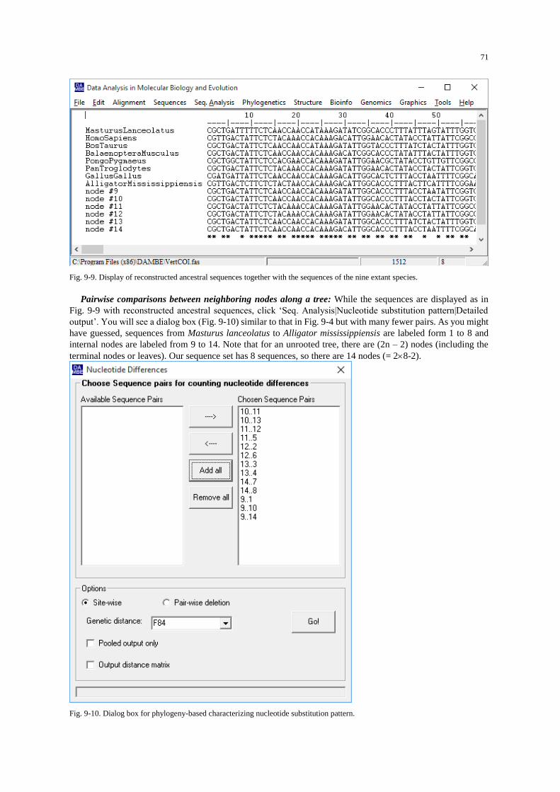
71
Fig. 9-9. Display of reconstructed ancestral sequences together with the sequences of the nine extant species.
Pairwise comparisons between neighboring nodes along a tree: While the sequences are displayed as in
Fig. 9-9 with reconstructed ancestral sequences, click ‘Seq. Analysis|Nucleotide substitution pattern|Detailed
output’. You will see a dialog box (Fig. 9-10) similar to that in Fig. 9-4 but with many fewer pairs. As you might
have guessed, sequences from Masturus lanceolatus to Alligator mississippiensis are labeled form 1 to 8 and
internal nodes are labeled from 9 to 14. Note that for an unrooted tree, there are (2n – 2) nodes (including the
terminal nodes or leaves). Our sequence set has 8 sequences, so there are 14 nodes (= 28-2).
Fig. 9-10. Dialog box for phylogeny-based characterizing nucleotide substitution pattern.
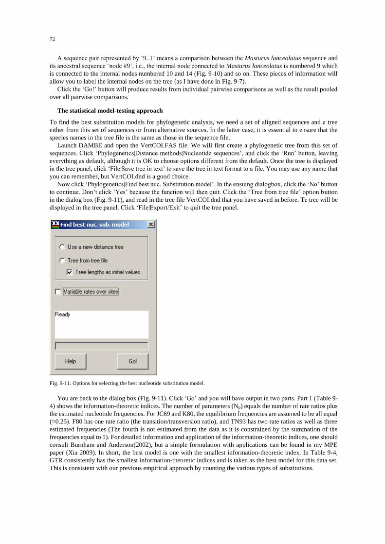
72
A sequence pair represented by ‘9..1’ means a comparison between the Masturus lanceolatus sequence and
its ancestral sequence ‘node #9’, i.e., the internal node connected to Masturus lanceolatus is numbered 9 which
is connected to the internal nodes numbered 10 and 14 (Fig. 9-10) and so on. These pieces of information will
allow you to label the internal nodes on the tree (as I have done in Fig. 9-7).
Click the ‘Go!’ button will produce results from individual pairwise comparisons as well as the result pooled
over all pairwise comparisons.
The statistical model-testing approach
To find the best substitution models for phylogenetic analysis, we need a set of aligned sequences and a tree
either from this set of sequences or from alternative sources. In the latter case, it is essential to ensure that the
species names in the tree file is the same as those in the sequence file.
Launch DAMBE and open the VertCOI.FAS file. We will first create a phylogenetic tree from this set of
sequences. Click ‘Phylogenetics|Distance methods|Nucleotide sequences’, and click the ‘Run’ button, leaving
everything as default, although it is OK to choose options different from the default. Once the tree is displayed
in the tree panel, click ‘File|Save tree in text’ to save the tree in text format to a file. You may use any name that
you can remember, but VertCOI.dnd is a good choice.
Now click ‘Phylogenetics|Find best nuc. Substitution model’. In the ensuing dialogbox, click the ‘No’ button
to continue. Don’t click ‘Yes’ because the function will then quit. Click the ‘Tree from tree file’ option button
in the dialog box (Fig. 9-11), and read in the tree file VertCOI.dnd that you have saved in before. Te tree will be
displayed in the tree panel. Click ‘File|Export/Exit’ to quit the tree panel.
Fig. 9-11. Options for selecting the best nucleotide substitution model.
You are back to the dialog box (Fig. 9-11). Click ‘Go’ and you will have output in two parts. Part 1 (Table 9-
4) shows the information-theoretic indices. The number of parameters (Np) equals the number of rate ratios plus
the estimated nucleotide frequencies. For JC69 and K80, the equilibrium frequencies are assumed to be all equal
(=0.25). F80 has one rate ratio (the transition/transversion ratio), and TN93 has two rate ratios as well as three
estimated frequencies (The fourth is not estimated from the data as it is constrained by the summation of the
frequencies equal to 1). For detailed information and application of the information-theoretic indices, one should
consult Burnham and Anderson(2002), but a simple formulation with applications can be found in my MPE
paper (Xia 2009). In short, the best model is one with the smallest information-theoretic index. In Table 9-4,
GTR consistently has the smallest information-theoretic indices and is taken as the best model for this data set.
This is consistent with our previous empirical approach by counting the various types of substitutions.
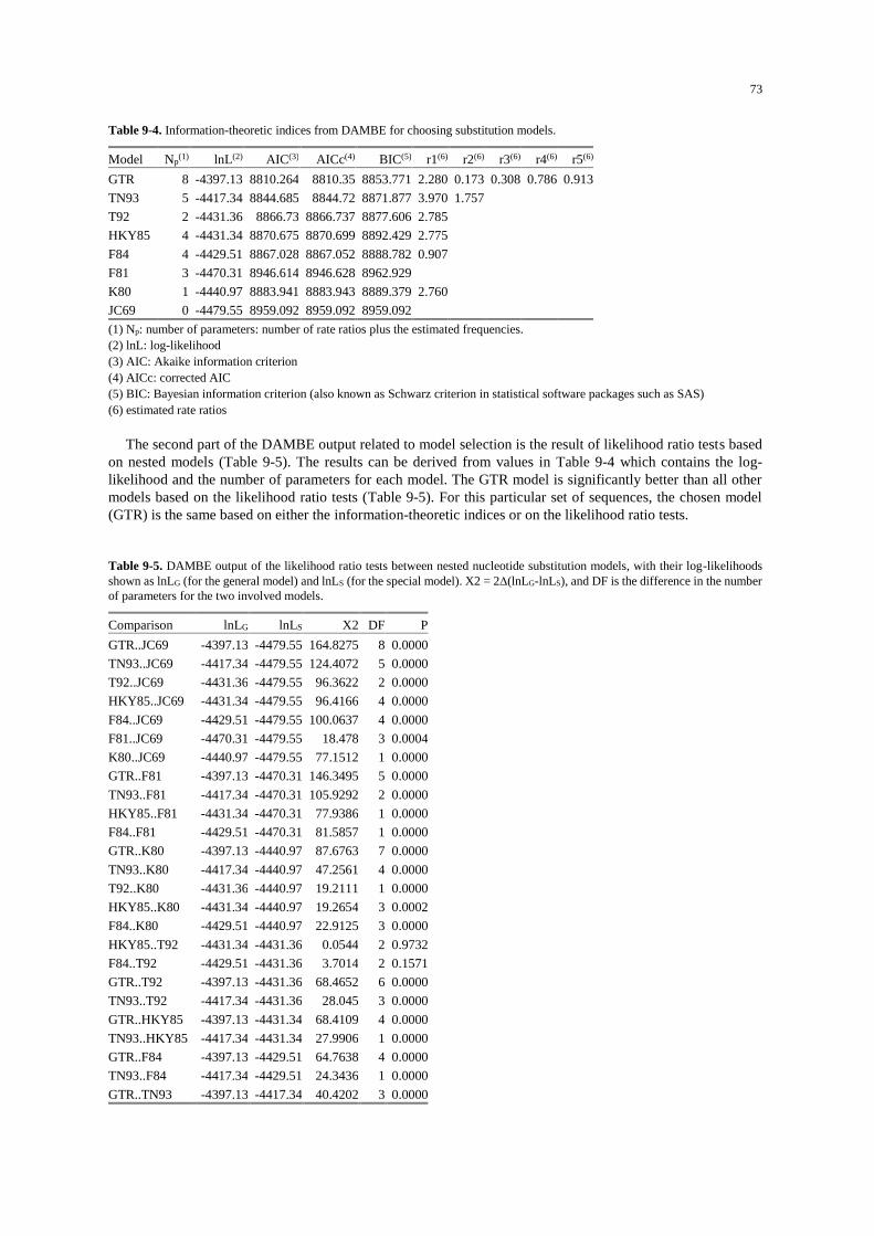
73
Table 9-4. Information-theoretic indices from DAMBE for choosing substitution models.
Model Np(1) lnL(2) AIC(3) AICc(4) BIC(5) r1(6) r2(6) r3(6) r4(6) r5(6)
GTR 8 -4397.13 8810.264 8810.35 8853.771 2.280 0.173 0.308 0.786 0.913
TN93 5 -4417.34 8844.685 8844.72 8871.877 3.970 1.757
T92 2 -4431.36 8866.73 8866.737 8877.606 2.785
HKY85 4 -4431.34 8870.675 8870.699 8892.429 2.775
F84 4 -4429.51 8867.028 8867.052 8888.782 0.907
F81 3 -4470.31 8946.614 8946.628 8962.929
K80 1 -4440.97 8883.941 8883.943 8889.379 2.760
JC69 0 -4479.55 8959.092 8959.092 8959.092
(1) Np: number of parameters: number of rate ratios plus the estimated frequencies.
(2) lnL: log-likelihood
(3) AIC: Akaike information criterion
(4) AICc: corrected AIC
(5) BIC: Bayesian information criterion (also known as Schwarz criterion in statistical software packages such as SAS)
(6) estimated rate ratios
The second part of the DAMBE output related to model selection is the result of likelihood ratio tests based
on nested models (Table 9-5). The results can be derived from values in Table 9-4 which contains the log-
likelihood and the number of parameters for each model. The GTR model is significantly better than all other
models based on the likelihood ratio tests (Table 9-5). For this particular set of sequences, the chosen model
(GTR) is the same based on either the information-theoretic indices or on the likelihood ratio tests.
Table 9-5. DAMBE output of the likelihood ratio tests between nested nucleotide substitution models, with their log-likelihoods
shown as lnLG (for the general model) and lnLS (for the special model). X2 = 2(lnLG-lnLS), and DF is the difference in the number
of parameters for the two involved models.
Comparison lnLG lnLS X2 DF P
GTR..JC69 -4397.13 -4479.55 164.8275 8 0.0000
TN93..JC69 -4417.34 -4479.55 124.4072 5 0.0000
T92..JC69 -4431.36 -4479.55 96.3622 2 0.0000
HKY85..JC69 -4431.34 -4479.55 96.4166 4 0.0000
F84..JC69 -4429.51 -4479.55 100.0637 4 0.0000
F81..JC69 -4470.31 -4479.55 18.478 3 0.0004
K80..JC69 -4440.97 -4479.55 77.1512 1 0.0000
GTR..F81 -4397.13 -4470.31 146.3495 5 0.0000
TN93..F81 -4417.34 -4470.31 105.9292 2 0.0000
HKY85..F81 -4431.34 -4470.31 77.9386 1 0.0000
F84..F81 -4429.51 -4470.31 81.5857 1 0.0000
GTR..K80 -4397.13 -4440.97 87.6763 7 0.0000
TN93..K80 -4417.34 -4440.97 47.2561 4 0.0000
T92..K80 -4431.36 -4440.97 19.2111 1 0.0000
HKY85..K80 -4431.34 -4440.97 19.2654 3 0.0002
F84..K80 -4429.51 -4440.97 22.9125 3 0.0000
HKY85..T92 -4431.34 -4431.36 0.0544 2 0.9732
F84..T92 -4429.51 -4431.36 3.7014 2 0.1571
GTR..T92 -4397.13 -4431.36 68.4652 6 0.0000
TN93..T92 -4417.34 -4431.36 28.045 3 0.0000
GTR..HKY85 -4397.13 -4431.34 68.4109 4 0.0000
TN93..HKY85 -4417.34 -4431.34 27.9906 1 0.0000
GTR..F84 -4397.13 -4429.51 64.7638 4 0.0000
TN93..F84 -4417.34 -4429.51 24.3436 1 0.0000
GTR..TN93 -4397.13 -4417.34 40.4202 3 0.0000
74
More questions
1. If you have a set of aligned nucleotide sequences that differ substantially in nucleotide frequencies, e.g., one
has frequencies for A, C, G and T equal to 0.1, 0.4, 0.4, 0.1, respectively, and another has corresponding
frequencies equal to 0.4, 0.1, 0.1, 0.4, what substitution model would be appropriate for describing the
substitution process involving the sequences? (Answer: This excludes all time-reversible models. One should
use a substitution model for non-stationary process.)
2. If a set of aligned sequences has equal nucleotide frequencies but transitions occur much more frequently
than transversions, which substitution model would be appropriate for phylogenetic analysis of these
sequences?
3. You examined nucleotide frequencies of a set of aligned sequences. Every sequence has A, C, G, and T
frequencies close to 0.1, 0.4, 0.4, and 0.1, respectively. Without checking substitution patterns, what
substitution models would be inappropriate and what might be appropriate for the sequences?
4. Why would transversions outnumber transitions in sequences that have experienced full substitution
saturation? What is the expected number of transitions over transversions for sequences having experienced
full substitution saturation, assuming equal nucleotide frequencies?
5. CpG-specific methyltransferase methylates the C in CpG dinucleotide and increase the CpG TpG
transitions. DNA methylation activity is low in invertebrate genomes but high in vertebrate genomes. If you
are studying a set of aligned sequences including both invertebrate and vertebrate species, what substitution
model would be appropriate for modeling the evolutionary process?
6. What are the main advantages of using information-theoretic indices over the likelihood ratio test?
75
LAB 10 MOLECULAR PHYLOGENETICS
Introduction
Molecular phylogenetics has two objectives (Fig. 10-1): 1) characterizing the branching patterns (cladogenic
events, specifically the speciation and gene duplication events) in evolution, and 2) dating of these speciation or
gene duplication events that may help us understand functional divergence of genes. Phylogenetics can also help
us to identify common ancestors such as the mitochondrial “Eve” (because mitochondrial genomes are
maternally inherited) or the Y-chromosome “Adam” (because Y-chromosome is passed down from father to
son). The universal common ancestor for all living organisms is termed cenancestor which may or may not be
identifiable (Xia and Yang 2013). In this laboratory we focus on the first objective, i.e., the characterization of
branching patterns (i.e., phylogenetic relationships).
One recent application of the phylogenetic methods by one of the former BPS4104 students is the elucidation
of the temporal sequence of gene duplication involving three paralogous genes, USP4, USP15 and USP11
(Vlasschaert, et al. 2015). Caitlyn Vlasschaert took BPS4104 in 2014, started her MSc with me in September
2014, and published her first paper in 2015.
Masturus lanceolatus
Bos taurus
Balaenoptera musculus
Pongo pygmaeus
Pan troglodytes
Homo sapiens
Gallus gallus
Alligator mississippiensis
Global clock?
Local clock?
No
Yes
Dating with a
global clock
No. Don't use the
data for dating
purposes
Yes
Dating with a
relaxed clock
Why not? Molecular
evolution studies to
find answer
Molecular data:
Sequences
Distances
Distance-based methods
Maximum parsimony
Maximum likelihood
Bayes method
Fig. 10-1. Outline of hypothesis testing concerning the molecular clock.
Major categories of phylogenetic methods
What are the molecular phylogenetic methods currently used to elucidate phylogenetic relationships? Four
categories of phylogenetic methods are widely used in molecular phylogenetics: the distance-based approach
popularized by MEGA {Kumar, 1993 #1209;Kumar, 2008 #29526}, the maximum parsimony (MP) approach
popularized by PAUP (Swofford 1993; Swofford 2000), the maximum likelihood (ML) approach popularized
by DNAML in the PHYLIP package (Felsenstein 2014) and the Bayesian inference (BI) popularized by
MrBayes and BEAST (Huelsenbeck and Ronquist 2001; Drummond and Rambaut 2007). The main difference
between ML and BI is that the former makes inferences entirely on the basis of information in the data, whereas
the latter makes inferences by incorporating prior information. While the BI approach has become increasingly
popular (Aris-Brosou and Xia 2008) and has contributed many phylogenetic trees in publications, I still have
not seen much contribution it makes towards resolving difficult phylogenetic controversies.
The plethora of sequence formats for phylogenetic analysis
Associated with the large number of phylogenetic methods is a proliferation of sequence formats. For
example, PHYLILP, MEGA, and PAUP all have their own sequence format. DAMBE reads and writes sequence
files in 25 standard sequence formats including the annotation-rich GenBank files, MEGA, PHYLIP, NEXUS,
FASTA, the binary trace files, and NeXML files (Vos, et al. 2012) for comparative sequence analysis. NeXML
76
format is an extensible sequence format for richly annotated comparative data to facilitate interoperability (Vos,
et al. 2012). This new data format was formulated with the participation of two Canadian scientists. It has already
been used for large-scale archiving of comparative data by TreeBASE (Boettiger and Lang 2012), and is likely
to become a standard in future evolutionary bioinformatic data analysis.
Phylogenetic methods we will learn in this lab
In this laboratory we will learn the distance-based, MP and ML methods used in molecular phylogenetics.
Instead of using MEGA, PAUP and DNAML, we will learn all this methods by using DAMBE because (1)
DAMBE features perhaps the most extensive implementation of distance-based methods, (2) it has a simple yet
extremely fast MP method, and (3) it implements DNAML with several enhancements. There are some major
differences among and within these different categories of methods. It is important to know the nuance of the
differences.
Distance-based methods
The distance-based methods always have two components, i.e., the estimation of the pairwise genetic distance
and the tree-building algorithm (e.g., UPGMA, neighbor-joining, Fitch-Margoliash and FastME) based on the
genetic distances. For this reason, the genetic distance and tree-building algorithm constitute the minimum
specification of a distance-based method in publication
The genetic distance: There are two approaches to estimate genetic distances, the independent estimation
(IE) approach and the simultaneous estimation (SE) approach, with distances obtained by the SE approach
performing much better in phylogenetic reconstruction than those obtained by the IE approach (Tamura, et al.
2004). There are two SE approaches, one based on the least-squares (LS) approach (Xia 2009) and the maximum
likelihood (ML) approach (Tamura, et al. 2004). The SE distance obtained with the ML approach is known as
the maximum composite likelihood distance, and is implemented in MEGA4 based on the TN93 substitution
model (Tamura, et al. 2007). The same distance is labeled as MLCompositeTN93 in DAMBE which also
implements the distance based on the F84 model, designated as MLCompositeF84. The corresponding distances
based on the LS approach for TN93 and F84 models are designated as LSCompositeTN93 and LSCompositeF84,
respectively, in DAMBE. The DNADist program in the PHYLIP package (Felsenstein 2014) represents an early
attempt to obtain genetic distances using the SE approach. It generates the MLCompositeF84 distance but
requires the user to input the transition/transversion ratio. It is important to keep in mind that a specification that
the genetic distance is computed with the F84 model (or TN93) is insufficient for publication because IE
distances based on the F84 model could be quite different from SE distances based on the same substitution
model.
The tree-building algorithm: The tree-building algorithm typically works in three steps. First a new
topology is generated. Second, branch lengths (bi) of the topology are evaluated, typically by the least-squares
method or by the Fitch-Margoliash method (Note that the Fitch-Margoliash method for branch length evaluation
is different from the Fitch-Margoliash criterion for choosing the best tree). Third, a criterion is computed so that
the algorithm can decide which tree is the best tree based on the criterion. Commonly used criteria in distance-
based methods are the minimum evolution criterion (i.e., a tree with the shortest tree length, which equals bi,
is the best tree) and the Fitch-Margoliash criterion (which consists of a set of slightly different least-squares
criteria, with the best tree having the smallest sum of squares). Distance-based trees built in this way are said to
be based on a global criterion, with examples including FastME and Fitch-Margoliash methods.
The neighbor-joining method uses the minimum evolution criterion, but the criterion is applied locally, not
globally. In other words, the algorithm does not build different fully resolved N-taxa trees and choose the shortest
tree as the best tree. Instead, it clusters two taxa together if that clustering leads to the shortest partially resolved
tree compared to other alternative two-taxa clustering. The UPGMA method is even more local in term of apply
the minimum evolution criterion – it groups any two taxa that have the shortest distance. Thus, theoretically, the
FastME method should produce better trees than the neighbor-joining method which in turn should outperform
the UPGMA method. In practice, the neighbor-joining performs extremely well.
The maximum parsimony (MP) method
The MP method, together with the maximum likelihood (ML) method, is character-based instead of distance-
based. The most advanced implementation of the MP method is PAUP (Swofford 1993; Swofford 2000). The
most parsimonious tree is one that can explain the nucleotide or amino acid differences in aligned sequences
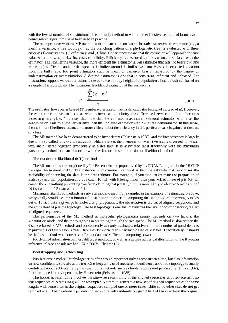
77
with the fewest number of substitutions. It is the only method in which the exhaustive search and branch-and-
bound search algorithms have been used in practice.
The main problem with the MP method is that it can be inconsistent. In statistical terms, an estimator (e.g., a
mean, a variance, a tree topology, i.e., the branching pattern of a phylogenetic tree) is evaluated with three
criteria: (1) consistency, (2) efficiency, and (3) bias. Consistency means that the estimator will approach the true
value when the sample size increases to infinity. Efficiency is measured by the variance associated with the
estimator. The smaller the variance, the more efficient the estimator is. An estimator that hits the bull’s eye (the
true value) is efficient, and one that spreads the bullets around the bull’s eye is not. Bias is the expected deviation
from the bull’s eye. For point estimators such as mean or variance, bias is measured by the degree of
underestimation or overestimation. A desired estimator is one that is consistent, efficient and unbiased. For
illustration, suppose we want to estimate the variance of body height of a population of male freshmen based on
a sample of n individuals. The maximum likelihood estimator of the variance is
2
2 1
( )n
i
i
x x
sn
(10.1)
The estimator, however, is biased (The unbiased estimator has its denominator being n-1 instead of n). However,
the estimator is consistent because, when n increases to infinity, the difference between n and n-1 becomes
increasing negligible. You may also note that the unbiased maximum likelihood estimator with n as the
denominator leads to a smaller variance than the unbiased estimator with n-1 as the denominator. In this sense,
the maximum likelihood estimator is more efficient, but the efficiency in this particular case is gained at the cost
of a bias.
The MP method has been demonstrated to be inconsistent (Felsenstein 1978), and the inconsistency is largely
due to the so-called long-branch attraction which refers to the phenomenon when two highly diverged non-sister
taxa are clustered together erroneously as sister taxa. It is associated most frequently with the maximum
parsimony method, but can also occur with the distance-based or maximum likelihood method.
The maximum likelihood (ML) method
The ML method was championed by Joe Felsenstein and popularized by his DNAML program in the PHYLIP
package (Felsenstein 2014). The criterion in maximum likelihood is that the estimate that maximizes the
probability of observing the data is the best estimate. For example, if you want to estimate the proportion of
males (p) in a fish population and you catch 10 fish with 5 being males, then your ML estimate of p is 0.5. Of
course there is nothing preventing you from claiming that p = 0.1, but it is more likely to observe 5 males out of
10 fish with p = 0.5 than with p = 0.1.
Maximum likelihood methods are always model-based. For example, in the example of estimating p above,
we typically would assume a binominal distribution in order to computing the likelihood of observing 5 males
out of 10 fish with a given p. In molecular phylogenetics, the observation is the set of aligned sequences, and
the equivalent of p is the topology. The best topology is one that maximizes the likelihood of observing the set
of aligned sequences.
The performance of the ML method in molecular phylogenetics mainly depends on two factors, the
substitution model and the thoroughness in searching through the tree space. The ML method is slower than the
distance-based or MP methods and consequently can only evaluate a relatively limited number of possible trees
in practice. For this reason, a “ML” tree may be worse than a distance-based or MP tree. Theoretically, it should
be the best method when one has sufficient data and sufficient computing power.
For detailed information on these different methods, as well as a simple numerical illustration of the Bayesian
inference, please consult my book (Xia 2007a, Chapter 13).
Bootstrapping and jackknifing
Publications in molecular phylogenetics often would report not only a reconstructed tree, but also information
on how confident we are about the tree. One frequently used measure of confidence about tree topology (actually
confidence about subtrees) is by the resampling methods such as bootstrapping and jackknifing (Efron 1982),
first introduced to phylogenetics by Felsenstein (Felsenstein 1985).
The bootstrap resampling involves the site-wise re-sampling of the aligned sequences with replacement, so
that sequences of N sites long will be resampled N times to generate a new set of aligned sequences of the same
length, with some sites in the original sequences sampled one or more times while some other sites do not get
sampled at all. The delete-half jackknifing technique will randomly purge off half of the sites from the original

78
sequences so that the new set of aligned sequences will be half as long as the original. Such resampling procedure
will typically be repeated a large number of times to generate a large number of new samples.
Each new sample (i.e., new set of aligned sequences), no matter whether it is from bootstrapping or
jackknifing, will then be subject to regular phylogenetic reconstruction. The frequencies of subtrees will then be
counted from reconstructed trees. If a subtree appears in all reconstructed trees, then the bootstrapping or
jackknifing value is 100% for that sub tree, i.e., the strongest possible support for the subtree.
Note that results from resampling (either bootstrapping or jackknifing) will typically not be the same,
especially with a small number of resampled data sets. The result will be more similar with increasing number
of resampled data sets
Although the bootstrap and the jackknife generally produce similar results, there are some subtle differences.
Suppose that we have a set of aligned sequences of N sites long. For the bootstrap resampling, the probability
of each site being sampled is 1/N, and the mean number of times a site gets sampled in each bootstrapping
resampling is simply one. Thus, a site gets sampled 0, 1, 2, ..., N times follows a Poisson distribution with a
mean equal to one. This implies that about 37% of the sites will not be sampled, while 63% of the sites will be
sampled at least once. In jackknifing, we have 50% of the sites not sampled and the other 50% of the sites
sampled just once. Thus, a jackknifed sample is expected to be less similar to the original sample than a
bootstrapped sample. Consequently, jackknifed samples may be less similar to each other than bootstrapped
samples.
Phylogenetic reconstruction with a global molecular clock
Molecular phylogenetics has two major objectives, i.e., elucidating the ancestor-descendent relationships among
different species and homologous genes, and dating speciation events and gene duplication events. Dating
assumes the existence of a molecular clock, either local or global. The existence of a global clock simplifies
much computation.
There are several methods that can generate a tree with a global clock. These include the distance-based
methods such as UPGMA and Kitsch (in the PHYLIP package) and maximum likelihood methods such as
DNAMLK (in the PHYLIP package). A tree with a molecular clock allows its branches to be calibrated by dated
fossils.
Objectives
Distance-based, MP and ML methods
Different phylogenetic reconstruction methods, with different criteria of choosing the tree, may produce different
trees, and are useful in different situations. You should keep in mind that all methods are good when they have
been used properly. You will develop an empirical appreciation of the strength and weakness of different
phylogenetic methods after this lab.
Bootstrap/ jackknife to evaluate subtree reliability
It is always desirable to know how well a phylogenetic tree is supported. There are two approaches to show how
a tree is supported. If you have several alternative trees and wish to know the relative statistical support of these
trees, then there are a variety of significance tests that can be used. On the other hand, if you wish to know how
well different subtrees are supported, then bootstrap or jackknife values are the most frequently used indices.
You will be able to attach bootstrap or jackknife values to subtrees after this lab, by using either distance-based,
maximum parsimony or maximum likelihood methods for phylogenetic reconstruction.
Phylogenetics assuming a global molecular clock
The distance-based method UPGMA always assumes a global molecular clock. One may also force a molecular
clock in the maximum likelihood framework. You will be able to use the UPGMA method or the maximum
likelihood method to construct trees with a global molecular clock after this lab.
Procedures
Two sequences files that we are going to use in this lab are included as sample files in the DAMBE installation
package. They contain mitochondrial COI and CytB gene sequences from eight vertebrate species (fish:
79
Masturus lanceolatus; human: Homo sapiens; cow: Bos Taurus; whale: Balaenoptera musculus; orangutan:
Pongo pygmaeus; chimpanzee: Pan troglodytes; chicken: Gallus gallus; alligator: Alligator mississippiensis).
The two files are in FASTA file format and can be found in DAMBE installation directory, typically C:\Program
Files\DAMBE for 32-bit PC or C:\Program Files (x86)\DAMBE for 64-bit PC:
1. VertCOI.FAS. This file contains aligned mitochondrial COI (cytochrome subunit I) sequences from the
eight vertebrate species,
2. VertCytB.FAS: This file contains unaligned mitochondrial Cyt-b (cytochrome b) sequences from the eight
vertebrate species. It is for you to practice nucleotide sequence alignment and codon sequence alignment guided
by aligned amino acid sequences.
Distance-based method
Phylogenetic reconstruction: To construct the phylogeny of the eight vertebrate species, read into DAMBE
the sequences in VertCOI.FAS by clicking ‘File|Open standard sequence file’ and open the VertCOI.FAS file.
Click ‘Phylogenetics|Distance methods|nucleotide sequences’. In the dialog box for you to set options, set the
genetic distance to the TN93 distance (the default in earlier versions of DABE), or MLCompositeTN93 (default
in latter versions), the tree-building algorithm to FastME (default), and Masturus lanceolatus as the outgroup.
Click the ‘Run’ button to build the tree. The resulting tree (Fig. 10-2) represents a well-corroborated
phylogenetic relationship among the eight species (‘well-corroborated’ is synonymous to ‘almost certainly
correct’). You may copy and paste the resulting tree to a PowerPoint slide.
PongoPygmaeus
PanTroglodytes
HomoSapiens
BalaenopteraMusculus
BosTaurus
AlligatorMississippiensis
GallusGallus
MasturusLanceolatus
MasturusLanceolatus
PongoPygmaeus
PanTroglodytesHomoSapiensBalaenopteraMusculus
BosTaurus
AlligatorMississippiensis
GallusGallus
(a) (b)
Fig. 10-2. Phylogenetic trees constructed with the TN93 distance, with the unrooted tree (a) from the FastME method and the rooted
tree (b) from UPGMA.
Now you may change options in two ways. One is by changing the tree-building algorithm, e.g., from FastME
that do not assume a molecular clock to UPGMA which assumes a global molecular clock. The tree built with
the UPGMA method is shown in Fig. 10-2b. The other is by changing genetic distances the simplest P distance
to the more complicated GTR distance (which is derived from the General Time Reversible substitution model).
Do these changes lead to the same tree?
Note that the UPGMA method assumes a global molecular clock, so all OTUs are of equal distance to the
root. Before we use any method that assumes a molecular clock, we typically would test the validity of the
molecular clock hypothesis first. There are two tests of the clock hypothesis, the relative-rate test and the tree-
based test. This topic is covered in another laboratory. If the clock hypothesis is not rejected, then we can use
dated fossils to derive divergence time between different species. Dating speciation events or gene duplication
events is a subject covered latter in the laboratory manual.
You can copy and paste the tree from DAMBE to PowerPoint slides or any other graphic programs including
EXCEL and WORD, either in fixed-resolution bitmapped format or in high-resolution Windows metafile format.
The latter should be used for formal presentation or publication. See Appendix 1 Copy trees from DAMBE to
PowerPoint slides for details.
In general, a set of sequences with strong phylogenetic signals will often be able to recover the true tree with
most combinations of tree-building algorithms and distances. Vertebrate mitochondrial COI is considered to
have strong phylogenetic signals and, for this reason, has been used in nearly all barcoding projects for
vertebrates.
The distance-based method is typically more resistant to the long-branch attraction problem haunting the
maximum parsimony method (Felsenstein 1978; Xia 2007a, pp. 277-279). However, distance-based methods
may also become inconsistent when distance estimation is biased. For example, underestimation of distances
will also lead to long-branch attraction for phylogenetic methods using either the minimum evolution criterion
or the Fitch-Margoliash criterion (Xia 2006).
A substitution model simpler than the true model will tend to underestimate the genetic distances between
OTUs, and such underestimation will be more severe between highly diverged OTUs than between closely

80
related OTUs. This will lead to long-branch attraction and wrong topology. For this reason, we should aim to
use genetic distances appropriate for the data to increase the accuracy of the genetic distances.
Bootstrapping and jackknifing: To do bootstrapping or jackknifing using the distance method on vertebrate
COI sequences, click ‘Phylogenetics|Distance methods|nucleotide sequences’. In the dialog box (Fig. 10-3), set
the distance to ‘TN93’ or ‘GTR’, outgroup to Masturus lanceolatus, and tree-building method to FastME (the
default). Check the ‘Resample (bootstrap, jackknife’ check box, and you will see the default resampling method
(bootstrapping) and the default number of resampled data sets (100).
Fig. 10-3. Setting options for generating a tree with bootstrap values.
Click the ‘Run’ button to obtain a tree with bootstrap values (Fig. 10-4). A value of 90 or higher associated
with a subtree is generally taken as strong statistical support for the subtree. You may now do resampling with
jackknife for comparison.
81
HomoSapiens
PanTroglodytes100
PongoPygmaeus
100
BosTaurus
BalaenopteraMusculus99
88
GallusGallus
AlligatorMississippiensis94
MasturusLanceolatus
Fig. 10-4. Distance-based tree (FastME on GTR distances) with bootstrap values in percentage.
Maximum parsimony (MP) method
Construct an MP tree: Click ‘Phylogenetics|Maximum parsimony|DNAMP’. A dialog box (Fig. 10-5)
appears for you to set the parameters. Again set Masturus lanceolatus as the outgroup. Don’t check the
‘Resampling Statistics’ check box. Click the ‘Go!’ button to perform the MP construction. DAMBE will report
to have found one most parsimonious tree, with 1427 steps. In terms of topology, this MP tree is identical to Fig.
10-2b.
Fig. 10-5. Dialog box for options in MP analysis.
Note that there is no explicit substitution model associated with the MP method because the MP method does
not explicitly assume a substitution model. However, sometimes a substitution process is assumed by using a
step matrix. The most frequently used step matrix treats transitions and transversions differently.
There is no commonly accepted way of treating indels in the MP and the ML method. The common practice
is to delete all indel-containing sites, as shown in Fig. 10-6. However, this approach has two problems. First,
DNA sequences often have conserved regions and variable regions. Few substitutions occur at conserved regions
which consequently contain little phylogenetic information. Most substitutions occur at the variable region.
Unfortunately, variable regions also often experience indel events, and the site-wise deletion of indel-containing
sites throws out the baby with the bath water. Second, recall that likelihood-based methods for nucleotide
sequences require a substitution model and estimated nucleotide frequencies. The nucleotide frequencies at the
variable regions should be the most relevant for computing likelihood. However, site-wise deletion of indel-
containing sites leave the nucleotide frequencies dominated by those of the conserved regions that often have
nucleotide frequencies different from those at the variable regions. You might also notice that, after deleting the
indel-containing sites, Seq1 and Seq3 have become identical, so are Seq2 and Seq4. Any phylogenetic program
will now group Seq1 with Seq3 and Seq2 with Seq4, contrary to what we would have expected by inspecting
the aligned sequences in the left of Fig. 10-6.

82
Seq1 AAC--GT--ACCGGTT
Seq2 AAC--GT--ACCAGTT
Seq3 AACCGGTTAACCGGTT
Seq4 AACCGGTTAACCAGTT
Seq1 AACGTACCGGTT
Seq2 AACGTACCAGTT
Seq3 AACGTACCGGTT
Seq4 AACGTACCAGTT
Fig. 10-6. Site-wise deletion of indel-containing sites.
In this context, the distance-based methods can use more information. For example, the genetic distance
between Seq3 and Seq4 (Fig. 10-6) can be calculated with all 16 sites instead of only 12 sites after the site-wise
deletion, and the variable sites do contribute to the nucleotide frequencies. How to make the best use of
information at indel-containing sites is still a hot research topic.
I should mention that keeping indel-containing sites may also lead to bias. For example, if one sequence has
experienced extensive deletion events at its variable sites so that almost all of its variable sites have been lost,
i.e., only conserved sites are left. The genetic distance between this sequence and all other sequences will
therefore be extraordinarily small whereas pairwise distances among those sequences with their variable sites
present will be relatively large. While this is a theoretically possible scenario, the problem has been rarely been
demonstrated (Van de Peer, et al. 1993).
Attach bootstrap/jackknife values to an MP tree: To generate a maximum parsimony tree with bootstrap
values, click ‘Phylogenetics|Maximum parsimony|DNAMP’. In the dialog box for you to set the parameters, set
Masturus lanceolatus as the outgroup. Check the ‘Resampling statistics’ check box, as is shown in Fig. 10-7.
Click the ‘Run’ button, and you will get a tree with bootstrap values similar to those in Fig. 10-4.
Fig. 10-7. Setting options for producing a maximum parsimony tree with bootstrap values in DAMBE.
Maximum likelihood (ML) reconstruction with bootstrap/jackknife
Read in the ‘VertCOI.FAS’ file and click ‘Phylogenetics|Maximum likelihood|DNAML’ to perform
phylogenetic analysis with the ML method. The substitution model is F84, which allows different transition and
transversion rates in the form of a transition/transversion ratio. You may specify such a ratio or let DAMBE
estimate the ratio (Fig. 10-8). Set the outgroup to 'MasturusLanceolatus' sequences. If you wish to produce a ML
tree with bootstrap values, you can check the ‘Resampling’ check box and specify either ‘Bootstrap’ or
‘Jackknife’ and the number of resampled data sets. Click the ‘Run’ button to run to build the tree. You should
obtain a tree with topology similar to that in Fig. 10-2a. If you wish to obtain bootstrap values, click the
‘Resample’ check box before clicking the ‘Run’ button.
83
Fig. 10-8. Setting options for phylogenetic analysis with the maximum likelihood method in DAMBE.
Work with the VertCytB.FAS file
The cytochrome-b gene in vertebrates is generally considered to have a weaker phylogenetic signal than the
COI gene. You will now explore this sequences by doing the following:
1. Read in the VertCytB.FAS file.
2. Align the sequences by clicking ‘Alignment|Align sequences by using ClustalW’
3. Using a distance-based method (e.g., FastME+MLCompositeF84), DNAMP and DNAML to reconstruct
the tree. Do the resulting trees show the same phylogenetic relationship as that in Fig. 10-2a?
4. Now read in VertCyb.FAS file again to replace the aligned sequences already in DAMBE’s buffer.
5. Translate into amino acid sequences.
6. Align the amino acid sequences
7. Click ‘Alignment|Align nuc. seq. to aligned AA seq in buffer’ and follow what you have done in a
previous laboratory on sequence alignment.
8. Using a distance-based method (e.g., FastME+MLCompositeF84), DNAMP and DNAML to reconstruct
the tree. Do the resulting trees show the same phylogenetic relationship as that in Fig. 10-2a?
9. In general, you will find that DNAML is better than the distance-based or maximum parsimony method.
Within distance methods, simultaneously estimated distances (e.g, MLCompositeF84 and
MLCompositeTN93) are better than independently estimated distances (e.g., F84 and TN93). However,
the former takes much longer to compute than the latter.

84
More questions
1. By which two categories of parameters do substitution models differ from each other?
Answer: Frequency parameters and rate parameters.
2. What approaches can we take to determine which substitution model is appropriate for our sequence data?
Answer: 1) empirical approach by counting the frequencies of different types of identical sites and different
sites and check whether transitions occurs more frequent than transversions, whether the two types of
transitions are different, etc., and 2) statistical approach for model selection by using information theoretic
indices or likelihood ratio test (if the models are nested).
3. Is a genetic distance based on a complicated substitution model always better than one based on a simple
model?
4. What are the key differences between UPGMA and FastME algorithms?
5. Use the following distance matrix to manually construct a UPGMA tree with branch lengths indicated on the
branches.
Gene1 Gene2 Gene3 Gene4 Gene5
Gene1 0.00 0.01 0.04 0.16 0.19
Gene2 0.00 0.03 0.14 0.17
Gene3 0.000 0.12 0.13
Gene4 0.00 0.02
Gene5 0.00
6. Given the following distance matrix and the topology for four species designated as S1-S4, evaluate the
branch lengths by using the least-square method, and compute the tree length.
Sp1
Sp2 0.3
Sp3 0.4 0.5
Sp4 0.4 0.6 0.6
7. Does a genetic distance such as the TN93 distance between two molecular sequences measure the divergence
time between the two sequences?
8. What does long-branch attraction mean? Is it a problem associated only with the maximum parsimony
method?
Answer: Long-branch attraction refers to the phenomenon in phylogenetics when two highly diverged non-
sister taxa are clustered together erroneously as sister taxa. It is associated most frequently with the maximum
parsimony method, but can occur with the distance-based or maximum likelihood method as well.
9. In distance-based method, is tree length the summation of all branch lengths or the summation of all pairwise
genetic distances?
10.Which four categories of phylogenetic methods are currently used?
Answer: 1) distance-based, 2) maximum parsimony, 3) maximum likelihood, 4) Bayesian inference.
11.Is transition probability matrix in a Markov chain a matrix of the probabilities of transitional substitutions?
12.Substitution models are the most fundamental in molecular phylogenetics. What are the major differences
between the JC69 model and the F84 model in terms of frequency and rate parameters?
13.When you produce your own bootstrapped tree, will the bootstrap values be the same as those in Fig. 4?
Explain why the bootstrap values on your tree could be different from those in Fig. 4. Will the difference
become smaller or larger when you increase the number of bootstrap samples (e.g., from the default 100 to
500)?
14.A biologist documented the following empirical substitution pattern after building a phylogenetic tree,
reconstructing the ancestral sequences, and performing pairwise sequence comparisons between neighboring
nodes. The values on the diagonal are number of sites where both sequences have identical nucleotides, and

85
those off-diagonal ones are number of differences, e.g., the value 20 corresponding to nucleotides A and G
means that there are 20 sites where one sequence is A and the other is G. What would be a suitable substitution
model for this set of sequences? Give reasons.
A G C T
A 3333 20 2 2
G 3322 3 3
C 3344 100
T 3323
86
LAB 11 TESTING THE MOLECULAR CLOCK HYPOTHESES
Introduction
Molecular phylogenetics has two objectives, one being the characterization of the branching patterns
(cladogenic events, specifically the speciation and gene duplication events) in evolution, and the other being the
dating of these speciation or gene duplication events. Dating assumes the existence of a molecular clock in which
each nucleotide or amino acid substitution is equivalent to a tick in a mechanical clock, although a tick in a
molecular clock often takes thousands of years or even longer.
Mutation and substitution
It is important to recognize the difference between mutation and substitution. A mutation is any change to the
genetic material such as DNA, whereas a substitution is the process whereby a new mutant allele completely
replaces the wild type allele in a population. Obviously, substitutions occur much less frequently than mutations.
Most mutations will be lost after only a few generations. A lethal mutation is lost within a single generation.
The probability of a new mutant allele eliminating all the alternative alleles and become "fixed" is termed
fixation probability. The rate of nucleotide substitution is the number of fixations occurring in a species per
nucleotide site per unit time. In genetics, a substitution is synonymous to a fixation event and substitution rate
is synonymous to fixation rate.
Different mutations may have very different fixation probabilities. If a mutation changes a functionally
important amino acid and disrupts the function of a key enzyme, then mutation is deleterious or even lethal, and
the mutant will leave few or no offspring (or said to be eliminated by negative or purifying selection). Such a
lethal mutation will have a fixation probability of 0. Only those individuals that do not carry the mutation will
survive to generate the next generation.
The molecular clock hypothesis
The molecular clock hypothesis claims that the substitution rate is roughly constant over time. However, many
factors can contribute to variation in substitution rate. In particular, the same nucleotide site can experience
different substitution rates during different geological time (heterotachy) or different nucleotide sites can have
different substitution rates (rate heterogeneity over sites).
Heterotachy: Heterotachy refers to the variation in substitution rates over time for a given site or a given
group of sites (Lopez, et al. 2002). Changes in functionally important amino acid sites are often deleterious, and
substitution rates at these sites are typically very low. However, sometime a dramatic environmental change may
favour some amino acid replacements, and these functionally important sites may experience a number of
changes in a short period of time in response to the changed selection pressure. Heterotachy is a chief contributor
to the violation of the molecular clock hypothesis.
Rate heterogeneity over sites: Functionally important sites typically evolve more slowly than functionally
unimportant sites. In protein-coding genes, the second codon position where any change will lead to
nonsynonymous substitutions (i.e., amino acid replacement) typically evolve much slower than the third codon
position where nucleotide changes will often be synonymous (Xia 1998b). These different sites represent
different molecular clocks.
For example, among 190 possible codon substitutions involving a single nucleotide change in the vertebrate
mitochondrial genetic code, 54 are transitions and 136 are transversions (Table 11-1). Among the 54 transitions,
26 are at the first codon positions with a mean Miyata’s distance (Miyata, et al. 1979) of 1.20. Miyata's distance
measures amino acid dissimilarity based on volume and polarity, with a larger value corresponding to greater
difference between the two amino acids. In contrast, 28 transitions are at the second codon position with a mean
Miyata’s distance equal to 2.16. In other words, transitions at the first codon position involve more similar amino
acid replacement than those at the second codon position. The same trend is visible with the 136 transversions
(Table 11-1).
All transitions at the third codon position are synonymous in vertebrate mitochondrial genomes. For the 24
nonsynonymous transversions at the third codon position, the mean Miyata’s distance (= 1.22, Table 11-1) is
close to that at the first codon position (= 1.49, Table 11-1). Thus, the second codon position is much more
functionally constrained than the third and the first codon positions in vertebrate mitochondrial genomes.
Consequently, the substitution rates at the first, second and third codon positions, designated r1, r2 and r3,
respectively, are typically in the pattern of r3 > r1 > r2.

87
Table 11-1. Distribution of transitions and transversions at the three codon positions for 190 possible codon substitutions involving
a single nucleotide change in vertebrate mitochondrial genomes. Generated from DAMBE.
CP(1) 1 2 3 Subtotal Prop
s(2) 26 28 0 54 0.2842
MeanD(3) 1.20 2.16 0.00 1.70
VarD(4) 0.73 0.54 0.00 0.85
v(5) 56 56 24 136 0.7158
MeanD(3) 1.49 2.36 1.22 1.80
VarD(4) 1.74 0.76 1.21 1.46
Sum 82 84 24 190
(1) CP: codon position
(2) s: transition
(3) MeanD: mean of Miyata’s distances
(4) VarD: variance of Miyata’s distances
(5) transversion
Rate heterogeneity over sites does not directly violate the molecular clock hypothesis. Whenever some sites
are functionally constrained, there is a chance for the sites to be more or less constrained in different lineages
experiencing different selection regimes. This will lead to violation of the molecular clock. In contrast, if all
sites are not constrained or only weakly constrained throughout evolutionary history, such as the third codon
position, then violation of the molecular clock is less likely. For this reason, third codon position should serve
as a better molecular clock than first or second codon positions. In any case, we need to test the molecular clock
hypothesis instead of assuming it.
Statistical tests of the molecular clock hypothesis
The relative-rate test: A relative-rate test is used when one is interested in testing whether two lineages are
evolving at the same rate. In principle, a relative-rate test involves only two ingroup taxa and one outgroup
taxon, and consequently does not require a tree. The purpose of the test is to find out whether the two ingroup
taxa have evolved at the same rate.
What are ingroup taxa? What is an outgroup? Ingroup taxa are the taxa we are interested in learning more,
e.g., the phylogenetic relationship among the taxa, the evolutionary rates among different lineages leading to
these taxa, etc. An outgroup is one or more species that does not belong to the ingroup. For example, if our
ingroup is made of primate species, then a species that is not a primate would be a valid outgroup (assuming that
primates form a monophyletic group). An ideal outgroup is not only an outgroup but also phylogenetic as close
as possible to the ingroup. For example, if our ingroup is made of the great apes, then both Escherichia coli and
Macaca mulatta (Rhesus monkey) are valid outgroups, but Rhesus monkey would make a much better outgroup
than E. coli. Thus, although a relative-rate test does not require a tree, it is very helpful to have a tree with the
two ingroups and species closely related to the ingroup for choosing a good outgroup.
Why should an ideal outgroup be closely related to the ingroup? You may get an intuitive understanding by
the following analogue. When I stand by the podium in a classroom, I can see that those students sitting in the
front row of seats are physically close to me than those sitting in the back row of seats. However, if I look at the
students in the classroom from 100 km away, then all what I see would be a blur, and it would be impossible to
tell which student is physically closer to me than others. The outgroup represents the position we stand to view
the two ingroups to see which one has evolved faster away from us. If our outgroup is E. coli, then the two
ingroups such as human and chimp would merge into a blur and the relative-rate test will often fail to give us
the correct answer as to which one has evolved faster. However, a rhesus monkey as a an outgroup will
substantially improve our resolution.
There are two relative-rate tests implemented in DAMBE, with one based on nucleotide substitution model
(Muse and Weir 1992) and the other on codon-based model (Muse and Gaut 1994). For the nucleotide-based
model, both the transitional substitution rate and the transversional substitution rate are tested. For the codon-
based model, both the synonymous substitution rate and the nonsynonymous substitution rate are tested.
The statistical rationale of a relative-rate test is illustrated in Fig. 11-1, where and are used to designate
transitional and transversional substitution rates, respectively. Assuming the HKY85 substitution model and a
molecular clock, we expect 1 = 2 and 1 = 2. We first test whether this model (Model 2 in Fig. 11-1) is
significantly worse than the general model (Model 1 in Fig. 11-1) that does not force 1 = 2 and 1 = 2. It is
clear that the two models are nested, i.e., Model 2 is a special case of Model 1 when 1 = 2 and 1 = 2, so a
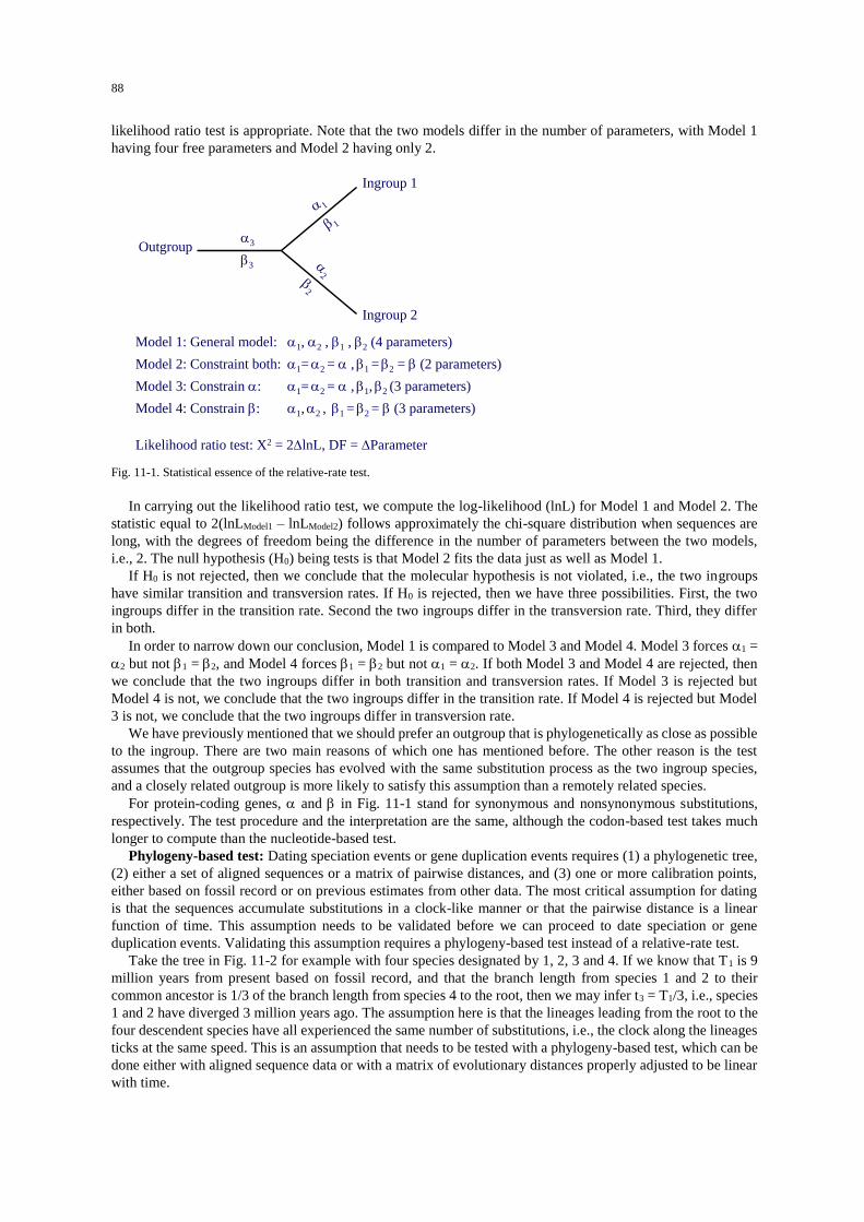
88
likelihood ratio test is appropriate. Note that the two models differ in the number of parameters, with Model 1
having four free parameters and Model 2 having only 2.
Outgroup
Ingroup 2
Ingroup 1
1
1
2
2
Model 1: General model: 1, 2 , 1 , 2 (4 parameters)
Model 2: Constraint both: 1=2 = ,1 =2 = (2 parameters)
Model 3: Constrain : 1=2 = ,1, 2 (3 parameters)
Model 4: Constrain : 1,2 , 1 =2 = (3 parameters)
Likelihood ratio test: X2 = 2lnL, DF = Parameter
3
3
Fig. 11-1. Statistical essence of the relative-rate test.
In carrying out the likelihood ratio test, we compute the log-likelihood (lnL) for Model 1 and Model 2. The
statistic equal to 2(lnLModel1 – lnLModel2) follows approximately the chi-square distribution when sequences are
long, with the degrees of freedom being the difference in the number of parameters between the two models,
i.e., 2. The null hypothesis (H0) being tests is that Model 2 fits the data just as well as Model 1.
If H0 is not rejected, then we conclude that the molecular hypothesis is not violated, i.e., the two ingroups
have similar transition and transversion rates. If H0 is rejected, then we have three possibilities. First, the two
ingroups differ in the transition rate. Second the two ingroups differ in the transversion rate. Third, they differ
in both.
In order to narrow down our conclusion, Model 1 is compared to Model 3 and Model 4. Model 3 forces 1 =
2 but not 1 = 2, and Model 4 forces 1 = 2 but not 1 = 2. If both Model 3 and Model 4 are rejected, then
we conclude that the two ingroups differ in both transition and transversion rates. If Model 3 is rejected but
Model 4 is not, we conclude that the two ingroups differ in the transition rate. If Model 4 is rejected but Model
3 is not, we conclude that the two ingroups differ in transversion rate.
We have previously mentioned that we should prefer an outgroup that is phylogenetically as close as possible
to the ingroup. There are two main reasons of which one has mentioned before. The other reason is the test
assumes that the outgroup species has evolved with the same substitution process as the two ingroup species,
and a closely related outgroup is more likely to satisfy this assumption than a remotely related species.
For protein-coding genes, and in Fig. 11-1 stand for synonymous and nonsynonymous substitutions,
respectively. The test procedure and the interpretation are the same, although the codon-based test takes much
longer to compute than the nucleotide-based test.
Phylogeny-based test: Dating speciation events or gene duplication events requires (1) a phylogenetic tree,
(2) either a set of aligned sequences or a matrix of pairwise distances, and (3) one or more calibration points,
either based on fossil record or on previous estimates from other data. The most critical assumption for dating
is that the sequences accumulate substitutions in a clock-like manner or that the pairwise distance is a linear
function of time. This assumption needs to be validated before we can proceed to date speciation or gene
duplication events. Validating this assumption requires a phylogeny-based test instead of a relative-rate test.
Take the tree in Fig. 11-2 for example with four species designated by 1, 2, 3 and 4. If we know that T1 is 9
million years from present based on fossil record, and that the branch length from species 1 and 2 to their
common ancestor is 1/3 of the branch length from species 4 to the root, then we may infer t3 = T1/3, i.e., species
1 and 2 have diverged 3 million years ago. The assumption here is that the lineages leading from the root to the
four descendent species have all experienced the same number of substitutions, i.e., the clock along the lineages
ticks at the same speed. This is an assumption that needs to be tested with a phylogeny-based test, which can be
done either with aligned sequence data or with a matrix of evolutionary distances properly adjusted to be linear
with time.
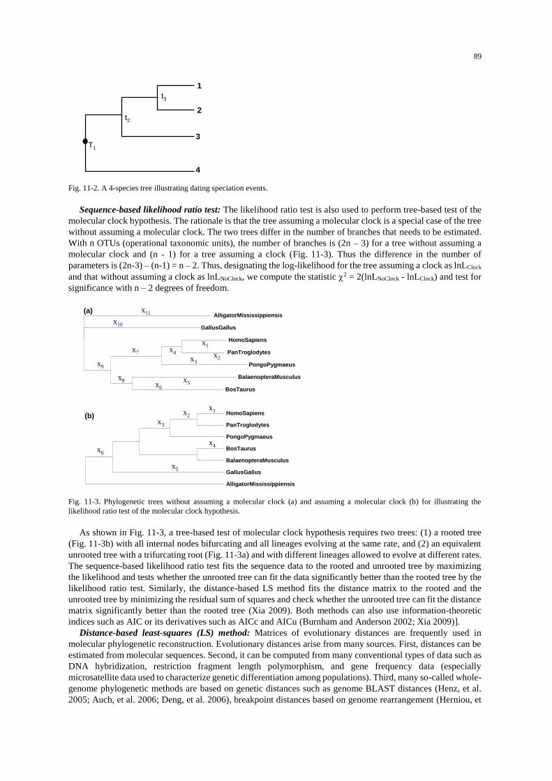
89
t3
t2
T1
4
2
1
3
Fig. 11-2. A 4-species tree illustrating dating speciation events.
Sequence-based likelihood ratio test: The likelihood ratio test is also used to perform tree-based test of the
molecular clock hypothesis. The rationale is that the tree assuming a molecular clock is a special case of the tree
without assuming a molecular clock. The two trees differ in the number of branches that needs to be estimated.
With n OTUs (operational taxonomic units), the number of branches is (2n – 3) for a tree without assuming a
molecular clock and (n - 1) for a tree assuming a clock (Fig. 11-3). Thus the difference in the number of
parameters is (2n-3) – (n-1) = n – 2. Thus, designating the log-likelihood for the tree assuming a clock as lnLClock
and that without assuming a clock as lnLNoClock, we compute the statistic 2 = 2(lnLNoClock - lnLClock) and test for
significance with n – 2 degrees of freedom.
BosTaurus
BalaenopteraMusculus
PongoPygmaeus
PanTroglodytes
HomoSapiens
GallusGallus
AlligatorMississippiensis
x1
x5
x7 x2
x6
x5
x4
x3
x2
x6
x1x4
x3
x8
x10
x11
x9
AlligatorMississippiensis
GallusGallus
BalaenopteraMusculus
BosTaurus
PongoPygmaeus
PanTroglodytes
HomoSapiens
(a)
(b)
Fig. 11-3. Phylogenetic trees without assuming a molecular clock (a) and assuming a molecular clock (b) for illustrating the
likelihood ratio test of the molecular clock hypothesis.
As shown in Fig. 11-3, a tree-based test of molecular clock hypothesis requires two trees: (1) a rooted tree
(Fig. 11-3b) with all internal nodes bifurcating and all lineages evolving at the same rate, and (2) an equivalent
unrooted tree with a trifurcating root (Fig. 11-3a) and with different lineages allowed to evolve at different rates.
The sequence-based likelihood ratio test fits the sequence data to the rooted and unrooted tree by maximizing
the likelihood and tests whether the unrooted tree can fit the data significantly better than the rooted tree by the
likelihood ratio test. Similarly, the distance-based LS method fits the distance matrix to the rooted and the
unrooted tree by minimizing the residual sum of squares and check whether the unrooted tree can fit the distance
matrix significantly better than the rooted tree (Xia 2009). Both methods can also use information-theoretic
indices such as AIC or its derivatives such as AICc and AICu (Burnham and Anderson 2002; Xia 2009)].
Distance-based least-squares (LS) method: Matrices of evolutionary distances are frequently used in
molecular phylogenetic reconstruction. Evolutionary distances arise from many sources. First, distances can be
estimated from molecular sequences. Second, it can be computed from many conventional types of data such as
DNA hybridization, restriction fragment length polymorphism, and gene frequency data (especially
microsatellite data used to characterize genetic differentiation among populations). Third, many so-called whole-
genome phylogenetic methods are based on genetic distances such as genome BLAST distances (Henz, et al.
2005; Auch, et al. 2006; Deng, et al. 2006), breakpoint distances based on genome rearrangement (Herniou, et
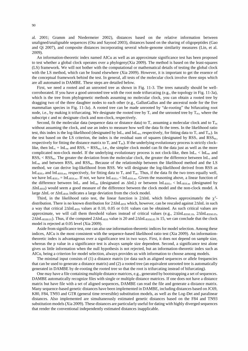
90
al. 2001; Gramm and Niedermeier 2002), distances based on the relative information between
unaligned/unalignable sequences (Otu and Sayood 2003), distances based on the sharing of oligopeptides (Gao
and Qi 2007), and composite distances incorporating several whole-genome similarity measures (Lin, et al.
2009).
An information-theoretic index named AICu as well as an approximate significance test has been proposed
to test whether a global clock operates over a phylogeny(Xia 2009). The method is based on the least-squares
(LS) framework. We will not bother with the computational or mathematical details of testing the global clock
with the LS method, which can be found elsewhere (Xia 2009). However, it is important to get the essence of
the conceptual framework behind the test. In general, all tests of the molecular clock involve three steps which
are all automated in DAMBE. These steps are detailed below.
First, we need a rooted and an unrooted tree as shown in Fig. 11-3. The trees naturally should be well-
corroborated. If you have a good unrooted tree with the root node trifurcating (e.g., the topology in Fig. 11-3a),
which is the tree from phylogenetic methods assuming no molecular clock, you can obtain a rooted tree by
dragging two of the three daughter nodes to each other (e.g., GallusGallus and the ancestral node for the five
mammalian species in Fig. 11-3a). A rooted tree can be made unrooted by “de-rooting” the bifurcating root
node, i.e., by making it trifurcating. We designate the rooted tree by Tc and the unrooted tree by Tnc, where the
subscript c and nc designate clock and non-clock, respectively.
Second, fit the molecular data (sequence data or distance data) to Tc assuming a molecular clock and to Tnc
without assuming the clock, and use an index to measure how well the data fit the trees. In the likelihood ratio
test, this index is the log-likelihood (designated by lnLc and lnLnc, respectively, for fitting data to Tc and Tnc). In
the test based on the LS criterion, the index is the residual sum of squares (designated by RSSc and RSSnc,
respectively for fitting the distance matrix to Tc and Tnc). If the underlying evolutionary process is strictly clock-
like, then lnLc = lnLnc and RSSc = RSSnc, i.e., the simpler clock model can fit the data just as well as the more
complicated non-clock model. If the underlying evolutionary process is not clock-like, then lnLc < lnLnc and
RSSc < RSSnc. The greater the deviation from the molecular clock, the greater the difference between lnLc and
lnLnc and between RSSc and RSSnc. Because of the relationship between the likelihood method and the LS
method, we can derive log-likelihood from RSS. We will designate the log-likelihood derived from RSS as
lnLRSS.c and lnLRSS.nc, respectively, for fitting data to Tc and Tnc. Thus, if the data fit the two trees equally well,
we have lnLRSS.c = lnLRSS.nc. If not, we have lnLRSS.c < lnLRSS.nc. Given the reasoning above, a linear function of
the difference between lnLc and lnLnc (designated as lnL) or between lnLRSS.c < lnLRSS.nc (designated by
lnLRSS) would seem a good measure of the difference between the clock model and the non-clock model. A
large lnL or lnLRSS indicates a large deviation from the clock model.
Third, in the likelihood ratio test, the linear function is 2lnL which follows approximately the 2-
distribution. There is no known distribution for 2lnLRSS which, however, can be rescaled against 2lnL in such
a way that critical 2lnLRSS values at 0.10, 0.05 or 0.01 values can be obtained. As such critical values are
approximate, we will call them threshold values instead of critical values (e.g., 2lnLRSS0.10, 2lnLRSS0.05,
2lnLRSS0.01). Thus, if the computed 2lnLRSS value is 20 and 2lnLRSS0.05 is 15, we can conclude that the clock
model is rejected at 0.05 level (Xia 2009).
Aside from significance test, one can also use information-theoretic indices for model selection. Among these
indices, AICu is the most consistent with the sequence-based likelihood ratio test (Xia 2009). An information-
theoretic index is advantageous over a significance test in two ways. First, it does not depend on sample size,
whereas the p value in a significance test is always sample size dependent. Second, a significance test alone
gives us little information when the null hypothesis is not rejected, but an information-theoretic index such as
AICu, being a criterion for model selection, always provides us with information to choose among models.
The minimal input consists of (1) a distance matrix (or data such as aligned sequences or allele frequencies
that can be used to generate a distance matrix) and (2) a rooted tree (an equivalent unrooted tree is automatically
generated in DAMBE by de-rooting the rooted tree so that the root is trifurcating instead of bifurcating).
One may have a file containing multiple distance matrices, e.g., generated by bootstrapping a set of sequences.
DAMBE automatically recognize files with single or multiple distance matrices. If one does not have a distance
matrix but have file with a set of aligned sequences, DAMBE can read the file and generate a distance matrix.
Many sequence-based genetic distances have been implemented in DAMBE, including distances based on JC69,
K80, F84, TN93 and GTR (general time reversible) substitution models, as well as the Log-Det and paralinear
distances. Also implemented are simultaneously estimated genetic distances based on the F84 and TN93
substitution models (Xia 2009). These distances are particularly useful for dating with highly diverged sequences
that render the conventional independently estimated distances inapplicable.

91
DAMBE can also read allele frequency data and generate a distance matrix. Three genetic distances are
available for conventional allele frequency data: Nei’s distance (Nei 1972), the chord distance (Cavalli-Sforza
and Edwards 1967), and the distance by Reynolds, Weir, and Cockerham (Reynolds, et al. 1983). For
microsatellite data, the distance based on a strict stepwise mutation model (Goldstein, et al. 1995; Slatkin 1995)
is implemented.
Here is a list of plain text files that come with DAMBE that you can use to practise the test the molecular
clock with the LS method:
1) VertCOI.fas which contains the mitochondrial COI gene from eight vertebrate species in FASTA format.
2) vertCOIRooted.dnd which contains a rooted tree in PHYLIP format.
Objectives
Learn to use DAMBE to perform relative-rate tests and to test the global clock hypothesis by using (1) the
distance-based method in the LS framework, and (2) sequence-based methods employing the likelihood ratio
test. The emphasis will be on the proper interpretation of the results rather than computational details.
Given the fact that the first and third codon positions of protein-coding genes are typically less functionally
constrained than the second codon position, we will examine whether the first and third codon position will
evolve in a more clock-like manner than the second codon position.
Procedures
The sequences that we will use in this laboratory are in the file VertCOI.fas file which is one of the sample files
that come with DAMBE. You will find it in DAMBE’s installation directory, typically C:\Program
Files\DAMBE. The file contains the coding sequence for the mitochondrial COI gene in eight vertebrate species
(Table 11-2). The 5’-end and the 3’-end of the coding sequences are difficult to align and have been deleted.
Table 11-2. Eight vertebrate species whose coding sequence for the mitochondrial COI gene are included in the VertCOI.FAS file
that comes with DAMBE.
Species Common name Accession(1)
Masturus lanceolatus Sharptail mola NC_005837
Homo sapiens Human NC_001807
Bos Taurus Cow NC_006853
Balaenoptera musculus Blue whale NC_001601
Pongo pygmaeus Orangutan NC_001646
Pan troglodytes Chimpanzee NC_001643
Gallus gallus Chicken NC_001323
Alligator mississippiensis American alligator NC_001922
(1) GenBank accession number of the mitochondrial genome from which the COI gene was extracted.
Start DAMBE and read in the aligned vertebrate mitochondrial gene sequences in the VertCOI.FAS file.
Construct a maximum likelihood tree by clicking "Phylogenetics|Maximum likelihood|DNAML". Choose
Masturus lanceolatus as outgroup and click the 'Run' button. You will get a tree that is identical to the one shown
in Fig. 11-4. The tree is important for us to choose a proper outgroup in relative-rate test.
PongoPygmaeus
PanTroglodytes
HomoSapiens
BalaenopteraMusculus
BosTaurus
AlligatorMississippiensis
GallusGallus
MasturusLanceolatus
Fig. 11-4. Maximum likelihood tree based on the COI sequences from eight vertebrate species, with the filled circle representing
the common ancestor of human (Homo sapliens) and orangutan (Pongo pygmaeus).
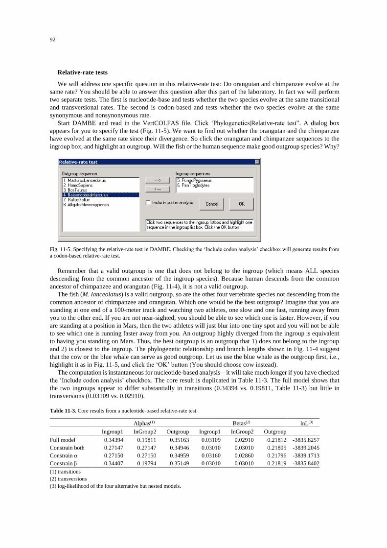
92
Relative-rate tests
We will address one specific question in this relative-rate test: Do orangutan and chimpanzee evolve at the
same rate? You should be able to answer this question after this part of the laboratory. In fact we will perform
two separate tests. The first is nucleotide-base and tests whether the two species evolve at the same transitional
and transversional rates. The second is codon-based and tests whether the two species evolve at the same
synonymous and nonsynonymous rate.
Start DAMBE and read in the VertCOI.FAS file. Click ‘Phylogenetics|Relative-rate test”. A dialog box
appears for you to specify the test (Fig. 11-5). We want to find out whether the orangutan and the chimpanzee
have evolved at the same rate since their divergence. So click the orangutan and chimpanzee sequences to the
ingroup box, and highlight an outgroup. Will the fish or the human sequence make good outgroup species? Why?
Fig. 11-5. Specifying the relative-rate test in DAMBE. Checking the ‘Include codon analysis’ checkbox will generate results from
a codon-based relative-rate test.
Remember that a valid outgroup is one that does not belong to the ingroup (which means ALL species
descending from the common ancestor of the ingroup species). Because human descends from the common
ancestor of chimpanzee and orangutan (Fig. 11-4), it is not a valid outgroup.
The fish (M. lanceolatus) is a valid outgroup, so are the other four vertebrate species not descending from the
common ancestor of chimpanzee and orangutan. Which one would be the best outgroup? Imagine that you are
standing at one end of a 100-meter track and watching two athletes, one slow and one fast, running away from
you to the other end. If you are not near-sighted, you should be able to see which one is faster. However, if you
are standing at a position in Mars, then the two athletes will just blur into one tiny spot and you will not be able
to see which one is running faster away from you. An outgroup highly diverged from the ingroup is equivalent
to having you standing on Mars. Thus, the best outgroup is an outgroup that 1) does not belong to the ingroup
and 2) is closest to the ingroup. The phylogenetic relationship and branch lengths shown in Fig. 11-4 suggest
that the cow or the blue whale can serve as good outgroup. Let us use the blue whale as the outgroup first, i.e.,
highlight it as in Fig. 11-5, and click the ‘OK’ button (You should choose cow instead).
The computation is instantaneous for nucleotide-based analysis – it will take much longer if you have checked
the ‘Include codon analysis’ checkbox. The core result is duplicated in Table 11-3. The full model shows that
the two ingroups appear to differ substantially in transitions (0.34394 vs. 0.19811, Table 11-3) but little in
transversions (0.03109 vs. 0.02910).
Table 11-3. Core results from a nucleotide-based relative-rate test.
Alphas(1) Betas(2) lnL(3)
Ingroup1 InGroup2 Outgroup Ingroup1 InGroup2 Outgroup
Full model 0.34394 0.19811 0.35163 0.03109 0.02910 0.21812 -3835.8257
Constrain both 0.27147 0.27147 0.34946 0.03010 0.03010 0.21805 -3839.2045
Constrain 0.27150 0.27150 0.34959 0.03160 0.02860 0.21796 -3839.1713
Constrain 0.34407 0.19794 0.35149 0.03010 0.03010 0.21819 -3835.8402
(1) transitions
(2) transversions
(3) log-likelihood of the four alternative but nested models.
93
The first likelihood ratio test we should do is to test the ‘Constrain both’ model (which is the model with a
molecular clock) against the full model, i.e., the null hypothesis (H0) that the constrained model can fit data just
as well as the full model. If H0 is not rejected, then we do not need to look at other models with intermediate
complexity. See Fig. 11-1 for the meaning of these models.
We compute 2 = 2 (lnLFull model – lnLConstrain both) = 6.757. With 2 degrees of freedom (why 2?), we have p =
0.03409. Recall that, for any significance test, the p value means the probability that we would be wrong if we
reject H0. As the p value is pretty small, we feel quite comfortable to reject H0 that the ‘Contrained both’ model
is equally good as the full model, i.e., we reject the molecular clock hypothesis. The test detail is also shown in
the computer output.
Now that H0 is rejected, we are left with three possibilities. First, the two ingroups differ in the transition rate.
Second, the two ingroups differ in the transversion rate. Third, they differ in both.
In order to narrow down our conclusion, the full model (Model 1 in Fig. 11-1) is compared to Model 3 and
Model 4 (Fig. 11-1). Model 3 forces 1 = 2 but not 1 = 2, and Model 4 forces 1 = 2 but not 1 = 2. If both
Model 3 and Model 4 are rejected, then we conclude that the two ingroups differ in both transition and
transversion rates. If Model 3 is rejected but Model 4 is not, we conclude that the two ingroups differ in the
transition rate, i.e., it is the differential transition rates that violate the molecular clock hypothesis. If Model 4 is
rejected but Model 3 is not, we conclude that the two ingroups differ in transversion rate, i.e., it is the differential
transversion rates that are responsible for the rejection of the molecular clock hypothesis.
The test of Model 3 and Model 4 against Model 1 is also presented in the computer output. However, you are
encouraged to compute 2, DF and p by yourself using results in Table 11-3. Once you have obtained 2 and
DF, you can use EXCEL to obtain p. For example, if your 2 = 6.691 and DF = 1, then you can obtain p by enter
‘=chidist(6.691,1)’ (without the single quotes) in any EXCEL cell. The test result will allow you to draw specific
conclusions as to whether the two in group species differ in transitions, in transversions, or in both.
You should now repeat the relative-rate test by including the codon-based analysis, i.e., by checking the
‘Include codon analysis’ checkbox in the dialog box in Fig. 11-5. Codon-based analysis is very slow and may
take several minutes. Alpha and beta in codon-based analysis refers to synonymous and nonsynonymous
substitutions, respectively. Run the test and make sure that you know how to answer the question of whether the
two ingroups evolve at the same synonymous and nonsynonymous rates.
Phylogeny-based tests
We will perform distance-based LS tests and sequence-based likelihood ratio tests. The former can be used with
either aligned sequences or distance matrices whereas the latter is for aligned sequences only. However, from a
statistical point of view, the latter uses more information in the sequences and should outperform the former
with aligned sequences. You should keep a comparative perspective when performing the two kinds of tests.
Distance-based method: The distance-based method has the advantage over sequence-based method in that
a distance matrix can not only be generated from sequences, but also from a variety of other types of data,
including allele frequency data, DNA hybridization data, RFLP data, microsatellite data, as well as genome-
based gene presence/absence data. We will compute evolutionary distances from aligned sequences and use a
rooted tree as input to test the molecular clock hypothesis by the LS method. A genetic distance matrix will be
generated from the aligned sequences for the testing purpose. Using a distance matrix generated from aligned
sequences facilitates the comparison between the distance-based and the sequence-based methods.
Start DAMBE. Click ‘File|Open standard sequence file’. In the file open dialog box, browse to DAMBE’s
installation directory (e.g., C:\Program Files\DAMBE), and double-click the “VertCOI.FAS” file (or single-
click to highlight it and then click the ‘Open’ button). In the next ‘Sequence Info’ dialog box, click ‘Protein-
coding Nuc. Seq.’ and choose the vertebrate mitochondrial translation table. Click ‘OK’ and the aligned
sequences will be displayed.
Click ‘Phylogenetics|Test molecular clock|Least-squares method|Nucleotide sequences’. The next dialog box
(Fig. 11-6) is for you to specify the rooted tree and the genetic distance to generate from the sequences. An
equivalent unrooted tree will be generated from the rooted tree that you specify.

94
Fig. 11-6. Option dialog box for testing the molecular clock hypothesis by the least-squares method.
You can input a rooted tree in two ways. We will use a tree that has already been generated and saved in the
file vertCOIRooted.dnd. However, if you do not have a tree but know what the topology should look like, you
can click the ‘New tree’ option button. This will bring up a tree panel with a star tree with OTUs being the names
of the sequences that have been read into DAMBE. You can then drag species or nodes to each other to form a
rooted tree.
For the time being, we will use the rooted tree in the vertCOIRooted.dnd file. Click ‘Tree from tree file’,
browse to DAMBE’s installation directory (e.g., C:\Program Files\DAMBE), and open the vertCOIRooted.dnd
file. The rooted tree will be displayed in the tree panel (Fig. 11-7). Note that it is a rooted tree with all nodes
bifurcating. Click ‘File|Export and exit’ to quit the tree panel. The tree-selection option in Fig. 11-2 is now
disabled.
Fig. 11-7. Tree panel for displaying or modifying topologies.

95
You generally should not allow negative branches. The power refers to the P parameter in the following
equation:
21
1 1
n nij ij
Pi j i ij
d eRSS
d
.......................................................................... (11.1)
where n is the number of species, dij is the observed distance between species i and j and eij is the expected
distance, computed as the length of the path linking species i and species j on the tree. The Fitch-Margoliash
criterion or least-square criterion is to find both branch lengths and tree topology that minimize RSS. It is better
to leave the default P = 0, i.e., the simple LS method.
In the genetic distance, I recommend to use one of the four simultaneously estimated (SE) distances, i.e.,
MLCompositeF84, MLCompositeTN93, MLCompositeF84, andMLCompositeTN93 (Xia 2009). If you are
using the third codon position only, then you often have no choice other than using these SE distances because
the conventional independently estimated distances often become inapplicable with highly diverged sequences.
Two such SE approaches have been implemented, one with the maximum likelihood method and the other
with the LS method. For the F84 model, they will estimate the transition/transversion ratio and use it for all
pairwise distance calculations. For the TN93 model, they will estimate the two transition/transversion ratio (1
and 2) and use them for all pairwise distance calculations. This approach avoids the inapplicable cases, and
produces much more robust distance estimates. These distances are implemented for the F84 and TN93
substitution models and designated ‘MLCompositeF84’, ‘MLCompositeTN93’, ‘LSCompositeF84’, and
‘LSCompositeTN93’ (where ML stands for maximum likelihood and LS stands for least-squares).
In this first try, we will not do resampling. So leave the resampling checkbox cleared and click the ‘Run’
button. The output is displayed, with some descriptions, a distance matrix, the re-evaluated rooted and unrooted
tree, and finally the result of the test of the molecular clock hypothesis (Table 11-4). The residual sum of squares
(RSS) for the clocked model is naturally greater than that for the non-clocked model (Table 11-4). However, the
non-clocked model entails more parameters. Can the increased fit of the tree to the distance matrix justify the
increased number of parameters? The resulting AICu for the clocked is smaller than that for the non-clocked
models, suggesting that the clocked model is better than the non-clocked model, i.e., the increased number of
parameters is not quite justifiable.
Table 11-4. Main output of the test of the molecular clock by the least-squares method based on a genetic distance.
Clock RSS NumParam AICu
Yes 0.003755 8 -6.5804
No 0.000701 14 -6.4015
For your practise, you can now re-run the test by checking the ‘Resample (bootstrap, jackknife) check box.
The default number of resampled data set is 100. The result (Fig. 11-8) shows that the mean AICu is smaller for
the clocked model than for the non-clocked model, although the two are not significantly different (p = 0.19645).
Also, 89% of the resampled data favour the clocked model.
Mean AICu (Clock) = -6.097555
Mean AICu (NoClock) = -5.568301
Mean Difference (D) = -0.529254
Std of D: = 0.409725
z score = -1.291731
p = 0.196450
89% of resampled data supports
the clock model.
Fig. 11-8. Output from the test of the molecular clock by the least squares method, with data resampling.
You may also evaluate the molecular clock separately for the first, second and third codon positions. It is
often assumed that the third codon position, being relatively free of the amino acid constraint, should evolve in
a more clock-like manner than the other two codon positions. You may have noted that, under DAMBE’s main
menu ‘Sequences’, there are submenus such as ‘Work on codon position 1’, ‘Work on codon position 1’ and
‘Work on codon position 3’. These allow you to extract specific codon positions. Once you have extracted one
codon position and have done the analysis with it, you may click ‘Sequences|Restore sequences’ to restore the
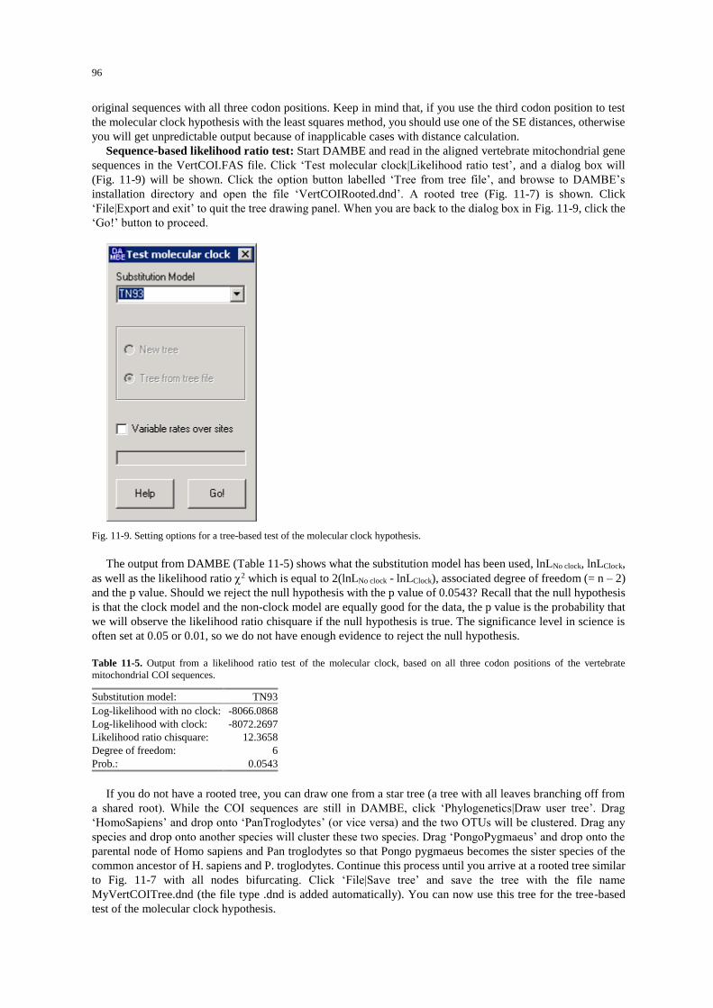
96
original sequences with all three codon positions. Keep in mind that, if you use the third codon position to test
the molecular clock hypothesis with the least squares method, you should use one of the SE distances, otherwise
you will get unpredictable output because of inapplicable cases with distance calculation.
Sequence-based likelihood ratio test: Start DAMBE and read in the aligned vertebrate mitochondrial gene
sequences in the VertCOI.FAS file. Click ‘Test molecular clock|Likelihood ratio test’, and a dialog box will
(Fig. 11-9) will be shown. Click the option button labelled ‘Tree from tree file’, and browse to DAMBE’s
installation directory and open the file ‘VertCOIRooted.dnd’. A rooted tree (Fig. 11-7) is shown. Click
‘File|Export and exit’ to quit the tree drawing panel. When you are back to the dialog box in Fig. 11-9, click the
‘Go!’ button to proceed.
Fig. 11-9. Setting options for a tree-based test of the molecular clock hypothesis.
The output from DAMBE (Table 11-5) shows what the substitution model has been used, lnLNo clock, lnLClock,
as well as the likelihood ratio 2 which is equal to 2(lnLNo clock - lnLClock), associated degree of freedom (= n – 2)
and the p value. Should we reject the null hypothesis with the p value of 0.0543? Recall that the null hypothesis
is that the clock model and the non-clock model are equally good for the data, the p value is the probability that
we will observe the likelihood ratio chisquare if the null hypothesis is true. The significance level in science is
often set at 0.05 or 0.01, so we do not have enough evidence to reject the null hypothesis.
Table 11-5. Output from a likelihood ratio test of the molecular clock, based on all three codon positions of the vertebrate
mitochondrial COI sequences.
Substitution model: TN93
Log-likelihood with no clock: -8066.0868
Log-likelihood with clock: -8072.2697
Likelihood ratio chisquare: 12.3658
Degree of freedom: 6
Prob.: 0.0543
If you do not have a rooted tree, you can draw one from a star tree (a tree with all leaves branching off from
a shared root). While the COI sequences are still in DAMBE, click ‘Phylogenetics|Draw user tree’. Drag
‘HomoSapiens’ and drop onto ‘PanTroglodytes’ (or vice versa) and the two OTUs will be clustered. Drag any
species and drop onto another species will cluster these two species. Drag ‘PongoPygmaeus’ and drop onto the
parental node of Homo sapiens and Pan troglodytes so that Pongo pygmaeus becomes the sister species of the
common ancestor of H. sapiens and P. troglodytes. Continue this process until you arrive at a rooted tree similar
to Fig. 11-7 with all nodes bifurcating. Click ‘File|Save tree’ and save the tree with the file name
MyVertCOITree.dnd (the file type .dnd is added automatically). You can now use this tree for the tree-based
test of the molecular clock hypothesis.
97
Do functionally unconstrained sites evolve more clock-like than functionally constrained sites?
We have just performed phylogeny-based likelihood ratio test of the molecular clock hypothesis, with all
three codon positions included (Table 11-5). We will now perform the same test, but separately for the three
codon positions. While the eight sequences of the VertCOI.FAS are displayed (1512 sites), click
‘Sequence|Work on codon position 1’ to get the first codon positions. Note that now you have only 504 sites.
Perform the likelihood ratio test on the first codon positions to obtain results similar to that in Table 11-5. To
get the second codon position, you need first to restore sequences so that you again will have 1512 sites in
DAMBE’s buffer, by first clicking ‘Sequence|Restore sequences’, and then click ‘Sequence|Work on codon
position 2’. Now perform the likelihood ratio test on the second codon positions. Do the same for the third codon
position. The results presented below are obtained with the TN93 model.
Test with the third codon position: Most substitutions at the third codon position are synonymous which
implies relatively weak purifying selection compared to first and second codon positions. For this reason,
evolutionary biologists tend to think that the third codon position should evolve in a more clock-like manner
than the first and second codon positions. Here we examine whether the third codon position of the COI gene
sequences evolve in a clock-like manner.
Read in the VertCOI.FAS file if you have not. Click ‘Sequences|Work on codon position 3’. You will note
that the aligned sequences are now only 1/3 of the original length because only the third codon positions are
shown. Click ‘Phylogenetics|Test molecular clock’ as before and use the same rooted tree file
‘VertCOIRooted.dnd’ to test the molecular clock.
Based on your test result, which should be similar to that in Table 11-6, what is the probability that we would
be wrong if we reject the null hypothesis? Keep in mind that most substitutions are at the third codon position.
Everything being equal, the third codon position should have greater statistical power to reject the null
hypothesis that the first and third codon positions. The observation that the null hypothesis is not rejected
confirms our prediction that the third codon position should evolve in a clock-like manner.
Table 11-6. Output from a likelihood ratio test of the molecular clock, based on the third codon position of the vertebrate
mitochondrial COI sequences.
Substitution model: TN93
Log-likelihood with no clock: -4006.4459
Log-likelihood with clock: -4010.8672
Likelihood ratio chisquare: 8.8426
Degree of freedom: 6
Prob.: 0.1826
Now repeat the test by using the distance-based LS method. Do you reach the same conclusion?
Click ‘Sequences|Restore Sequence’ to restore all three codon positions. Note that the sequences are again
1512 bases long.
Test with the first codon position: Recall that the first codon position is intermediate between the third and
the second codon positions in term of functional constraints. Most substitutions at the first codon positions are
nonsynonymous, but these synonymous substitutions involve more similar amino acids than those at the second
codon position.
Click ‘Sequences|Work on codon position 1’. You will note that the aligned sequences are again only 1/3 of
the original length because only the first codon positions are shown. Click ‘Phylogenetics|Test molecular clock’
as before and use the same rooted tree file ‘VertCOIRooted.dnd’ to test the molecular clock. Based on your test
result (Table 11-7), is the molecular hypothesis rejected?
Table 11-7. Output from a likelihood ratio test of the molecular clock, based on the first codon position of the vertebrate
mitochondrial COI sequences.
Substitution model: TN93
Log-likelihood with no clock: -1784.8591
Log-likelihood with clock: -1788.7016
Likelihood ratio chisquare: 7.685
Degree of freedom: 6
Prob.: 0.2621

98
You might ask why the p value (= 0.2621, Table 11-7) for the first codon position is greater than that for the
third codon position? Does this mean that the first codon position is even more clock-like than the third codon
position? The answer is no. As you might have noticed, the first codon position has much fewer substitutions
than the third codon position and consequently has limited power to reject the null hypothesis. However, the
result does suggest that the first codon position also evolve in a clock-like manner.
Now repeat the test by using the distance-based LS method. Do you reach the same conclusion?
Click ‘Sequences|Restore Sequence’ to restore all three codon positions. Note that the sequences are again
1512 bases long.
Test with the second codon position: Recall that the second codon position is the most constrained
functionally. Not only is any substitution at the second codon position nonsynonymous, but the nonsynonymous
substitutions also typically involve rather different amino acid replacement (Table 11-1). For this reason, we
expect the second codon position to evolve in the least clock-like manner.
Click ‘Sequences|Work on codon position 2’. You will note that the aligned sequences are again only 1/3 of
the original length because only the first codon positions are shown. Click ‘Phylogenetics|Test molecular clock’
as before and use the same rooted tree file ‘VertCOIRooted.dnd’ to test the molecular clock. Based on your test
result (Table 11-8), is the molecular hypothesis rejected?
Table 11-8. Output from a likelihood ratio test of the molecular clock, based on the second codon position of the vertebrate
mitochondrial COI sequences.
Substitution model: TN93
Log-likelihood with no clock: -978.2279
Log-likelihood with clock: -995.916
Likelihood ratio chisquare: 35.3763
Degree of freedom: 6
Prob.: 0
You may have noticed that few substitutions occur at the second codon position, i.e., it should have the least
statistical power to reject the null hypothesis, everything else being equal. The fact that the null hypothesis is
strongly rejected suggests that the second codon position must have evolved in strong violation of the molecular
clock hypothesis.
Now repeat the test by using the distance-based LS method. Do you reach the same conclusion? Which test
gives you a smaller p value? With two tests running on the same data, the test that gives you a smaller p value
is a more powerful (better) test.
You may also use the FastME method and the MLCompositeTN93 distance to build trees separately for the
first, second and third codon positions. Which tree appears to have different lineages evolving at the same rate?
Finally, I should emphasize that the null hypothesis tested in this laboratory is not that of constant
evolutionary rate, but is instead that of all extant OTUs are equidistance from the root. Thus, if all lineages
increase or decrease their evolutionary rate synchronously (which violates the clock hypothesis), this test will
not reject the clock hypothesis. However, one may argue that it must be extremely rare for different lineages to
increase or decrease their evolutionary rates synchronously. So the test is still a relevant test of the clock
hypothesis.
More questions
1. Give two reasons why an ideal outgroup should be phylogenetically close to the ingroup.
2. How is the likelihood-ratio chi-square calculated from the model-specific likelihood (or log-likelihood) in the
likelihood-ratio test? How is the associated degree of freedom calculated?
3. Use the VertCOI.fas file (containing mitochondrial COX1 sequences) for relative rate test between the cow
(Bos Taurus) and the whale (Balaenoptera musculus). Do the two evolve at the same transitional and
transversional rates? Do they evolve at the same synonymous and nonsynonymous rates? List output species
and provide statistical evidence for your conclusion.What kind of substitutions tend to violate the molecular
clock hypothesis?
4. Does molecular clock calibration always require dated fossils?
Answer: No. Tip-dating does not require dated fossils. Sometimes geographic events can also be used for
dating. For example, if we know the time of Africa-South America split to be 140 million years ago, then
species that originally were present at the border region would be split into two and have diverged

99
independently on the two continents 140 million years (assuming that they do not travel from one continent
to the other).
5. Do the tests of molecular clock we learned in this lab really test the molecular clock hypothesis? (Consider
the following scenario. Suppose all lineages evolve rapidly in one time period, and all evolve slowly in the
next period. This would violate the molecular clock hypothesis, but will our tests reveal such synchronous
increase or decrease in evolutionary rate?)

100
LAB 12 DATING WITH THE LEAST-SQUARES METHOD
Introduction
When did the vertebrates conquer the terrestrial environment? When did the ancestor of whales go back to the
marine environment? When did the haemoglobin gene family originate? When did the gene duplication events
occur that gave rise to and globin family? When did the HIV-1 virus jump the host to human? All these
questions can be addressed by dating in molecular phylogenetics.
There are two data-driven types of dating. The first uses fossil records as calibration points in internal nodes,
and the second is used specifically for dating rapidly evolving viruses sampled over years. The latter type is
typically referred to as tip-dating methods. I will refer to the first type as internal-calibration dating.
Many software packages can perform dating, with the most advanced and complicated being BEAST
(Drummond and Rambaut 2007). However, the complicated BEAST gives results similar to simpler distance-
based least squares (LS) methods (Xia and Yang 2011). In addition, BEAST performs dating with aligned
sequences, not distances, whereas the LS method can be used for both sequence data and distance data. So in
this laboratory we will practice the LS method for dating implemented in DAMBE.
Internal-calibration dating
Internal-calibration dating with the least-square method requires three pieces of data (1) a rooted tree, (2) a
set of data, either in the form of a set of aligned sequences or a distance matrix, that conform to the molecular
clock hypothesis, and (3) one or more calibration points from fossil record (e.g., the common ancestor of the
great apes, i.e., human, gorilla, chimpanzee and orang-utan walked on earth about 14 million years ago according
to fossil record). The calibration points allow us to translate branch lengths to absolute geological times.
Tip-dating
Tip-dating was originally developed for dating the divergence events in viral strains such as HIV viruses
sampled over years. The rationale is that, if the viral sequences evolve in a clock-like manner, then a viral strain
sampled in, say, year 1950, should have a shorter branch than its sister lineage sampled in, say, year 2000 from
their common ancestor. Thus, the sampling times can be used to calibrate the tree to obtain the divergence time
in different viral lineages. The method has been developed and applied successfully in dating HIV-1 sequences
and to settle questions concerning whether HIV-1 came to North America via Haiti or the other way round.
Tip-dating in DAMBE is developed in the least-square framework, based on evolutionary distances. Thus,
any data that can be used to generate evolutionary distances can be used for tip-dating. Such data include
molecular sequences, microsatellite or other allele frequency data, DNA hybridization, genome-based gene-
sharing or word-sharing data, etc. The only requirement is that the resulting pairwise distance increases roughly
linearly with time.
Objectives
There are two objectives in this tutorial. The first is to learn simple dating techniques to date speciation events,
gene duplication events or virus divergence events by using the LS method implemented in DAMBE. The second
is to learn how to attach confidence intervals to the estimated divergence time by using resampling methods
(bootstrap or jackknife).
Procedures
Internal-calibration dating
We will need to use four files: two sequence files and two tree files. These are all included in the DAMBE
installation package. They can be found in DAMBE installation directory, typically C:\Program Files\DAMBE:
mtDNAPri3.NEX: This file, in NEXUS format, contains third codon positions of the 12 protein-coding genes
collinear with the L-strand of vertebrate mitochondrial genome for seven great ape species. The sequences are
used in Rannala and Yang (2007), with two reasonably good calibration points.
mtDNAPri3F84SE.DIS, and mtDNAPri3F84SEMult.DIS: These two files, in PHYLIP format, contain
simultaneously estimated distances based on the F84 model from sequences in the mtDNAPri3.NEX file.
mtDNAPri3F84SE.DIS contains a single distance matrix, whereas mtDNAPri3F84SEMult.DIS contains 100
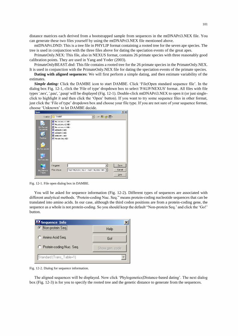
101
distance matrices each derived from a bootstrapped sample from sequences in the mtDNAPri3.NEX file. You
can generate these two files yourself by using the mtDNAPri3.NEX file mentioned above.
mtDNAPri.DND: This is a tree file in PHYLIP format containing a rooted tree for the seven ape species. The
tree is used in conjunction with the three files above for dating the speciation events of the great apes.
PrimateOnly.NEX: This file, also in NEXUS format, contains 26 primate species with three reasonably good
calibration points. They are used in Yang and Yoder (2003).
PrimateOnlyBEAST.dnd: This file contains a rooted tree for the 26 primate species in the PrimateOnly.NEX.
It is used in conjunction with the PrimateOnly.NEX file for dating the speciation events of the primate species.
Dating with aligned sequences: We will first perform a simple dating, and then estimate variability of the
estimates.
Simple dating: Click the DAMBE icon to start DAMBE. Click ‘File|Open standard sequence file’. In the
dialog box Fig. 12-1, click the 'File of type' dropdown box to select 'PAUP/NEXUS' format. All files with file
types '.nex', '.pau', '.paup' will be displayed (Fig. 12-1). Double-click mtDNAPri3.NEX to open it (or just single-
click to highlight it and then click the ‘Open’ button). If you want to try some sequence files in other format,
just click the ‘File of type’ dropdown box and choose your file type. If you are not sure of your sequence format,
choose ‘Unknown’ to let DAMBE decide.
Fig. 12-1. File open dialog box in DAMBE.
You will be asked for sequence information (Fig. 12-2). Different types of sequences are associated with
different analytical methods. ‘Protein-coding Nuc. Seq.” means protein-coding nucleotide sequences that can be
translated into amino acids. In our case, although the third codon positions are from a protein-coding gene, the
sequence as a whole is not protein-coding. So you should keep the default “Non-protein Seq.’ and click the ‘Go!’
button.
Fig. 12-2. Dialog for sequence information.
The aligned sequences will be displayed. Now click ‘Phylogenetics|Distance-based dating’. The next dialog
box (Fig. 12-3) is for you to specify the rooted tree and the genetic distance to generate from the sequences.
102
Fig. 12-3. Dialog box to specify options in distance-based dating.
You can input a rooted tree in two ways. We will use a tree that has already been generated and saved in the
file mtDNAPri.dnd. Click ‘Tree from tree file’ at the dialog box shown in Fig. 12-3, browse to DAMBE’s
installation directory (e.g., C:\Program Files\DAMBE), and open the mtDNAPri.dnd file. The rooted tree will
be displayed in the tree panel (Fig. 12-4). Note that it is a rooted tree with all nodes bifurcating.
Fig. 12-4. Tree panel for displaying or modifying topologies.
(If you want to use your own tree, make sure that the OTU names in the tree match those in the sequences. If
you do not have a tree but know what the topology should look like, you can click the ‘New tree’ option button.
This will bring up a tree panel with a star tree with OTUs being the names of the sequences that have been read
into DAMBE. You can then drag species or nodes to each other to form a rooted tree.)
You now need to specify calibration points. Note that all the internal nodes are numbered. Two calibration
points have been used for dating this set of sequences (Rannala and Yang 2007), one for the common ancestor
of all three great apes and human (node 8), and the other for the common ancestor of human and chimpanzee
(node 10). Right-click (Mac users: Enable the secondary click by go to ‘System Preferences|Keyboard & Mouse’
and set the right button to ‘Secondary Button’. The Mac default is to have both the left and right buttons set to
the same ‘Primary Button’. You may also set the tiny middle button, which defaults to ‘dashboard’, to the
secondary button) the node numbered ‘8’ (including human, two chimp species, gorilla and two orangutan
species), and enter 14 (for 14 million years ago) in the ensuing dialog box. Right-click the node numbered ‘10’
(including human, and two chimp species) and enter 7 (for 7 million years ago). Note that the calibration nodes

103
are now coloured in red. (You can click the tree in many different ways. Different clicks are often associated
with advanced dating functions. I have not finalized the interface. So click only as instructed.)
One should be aware of possible inconsistency in calibration points. Take Fig. 12-4 for example, if the
common ancestor for human and chimpanzee (node 10) was dated to be 14 million years old, whereas the
common ancestor for human, chimp, gorilla and orangutan (node 8) was dated to be less than 14 million years
old, then we have inconsistent calibration points. The dating algorithm will fail with inconsistent calibration
points.
Click ‘File|Export and exit’ to quit the tree panel. If you have forgotten to set the calibration points, DAMBE
will give you an opportunity to set them. If you have followed the instructions, the tree panel will close and the
tree-selection option in the dialog box (Fig. 12-3) will now be disabled because the selection is successful.
We have more options to set in the dialog box shown in Fig. 12-3. If you choose the ‘Hardbound’ option,
then the calibration times will be fixed. If you choose the ‘Softbound’ option, then the calibration points will be
changed to minimize the residual sum of squares when multiple calibration points are available. The ‘Softbound’
option will have no effect when there is only a single calibration point.
I suggest that you choose the ‘Softbound’ option. This is not only because the ‘Softbound’ option will lead
to smaller residual sum of squares, but also because fossil dating is often inaccurate. The ‘softbound’ option
allows the use of observed data to revise the calibration points. In a sense, the original calibration points may be
taken as a prior estimate, which is revised to give a posterior estimate by incorporating information from the
observed data.
In the genetic distance, the default is ‘MLCompositeF84’. This is one of the simultaneously estimated (SE)
distances for the F84 substitution model (Tamura, et al. 2004; Xia 2009). It is crucial to use SE distances,
especially when using the third codon position, because most of the independent estimation method will generate
inapplicable cases due to high sequence divergence.
Two such SE approaches have been implemented in DAMBE, one with the maximum likelihood method and
the other with the LS method (Xia 2009). These distances are implemented for the F84 and TN93 substitution
models in DAMBE and designated ‘MLCompositeF84’, ‘MLCompositeTN93’, ‘LSCompositeF84’, and
‘LSCompositeTN93’ (where ML stands for maximum likelihood and LS stands for least-squares). For the F84
model, a global transition/transversion ratio will be estimated and used for all pairwise distance calculations. For
the TN93 model, there are two transition/transversion ratios (1 and 2) which are used for all pairwise distance
calculations. This approach essentially eliminates the inapplicable cases, and produces much more robust
distance estimates.
In this first try, we will not do resampling. So leave the resampling checkbox cleared and click the ‘Run’
button. The output is displayed in two parts. The first is a tree with divergence time estimates (Fig. 12-5). Note
that the two calibration points are not 14 and 7 as we have inputted, but are 14.75 and 5.5, respectively. Had you
chosen "Hardbound' instead of ‘Softbound’ in the dialog box in Fig. 12-3, the two calibration nodes will show
exactly as the input values, i.e., 14 and 7, respectively. The option 'Softbound' allows DAMBE to fine-tune the
time of the calibration nodes by minimizing the sum of residual squares.
Fig. 12-5. Tree with estimated divergence time.
The tree can be manipulated in many ways and can be exported in low-resolution bitmapped .bmp format or
the high-resolution metafile format either for publication or PowerPoint presentation.
104
The second part is the text output, which includes the distance matrix, the estimated parameters of the
substitution model such as the transition/transversion ratio, log-likelihood for the distance estimation, and details
of the dating input and results such as the evolutionary rate, the tree with dates and the residual sum of squares
(RSS). RSS will be larger if you had chosen the ‘Hardbound’ option.
For your practise, you can now re-run the test by checking the ‘Hardbound’ option.
Estimating variability of the estimated divergence time: Now repeat the procedure until you get to the dialog
box shown in Fig. 12-3. Read in the mtDNAPri.DND tree and set the two calibration times as before. Now click
the ‘Resample (bootstrap, jackknife)’ check box. The default resampling protocol is ‘Bootstrap’ and the default
number of resampled data sets is 100. The higher the number, the better the estimates are. For practical research,
the number of resampled data sets should be at least 500. Click the ‘Run’ button.
After DAMBE has bootstrapped the specified number of times, dating results are again presented in two
parts: a tree (Fig. 12-6) with divergence times as well as text output. The tree differs from that in Fig. 12-5 in
that the standard deviation of the estimated divergence time is also presented.
It is important to keep in mind that the divergence time will be slightly different when you repeat the
bootstrapping procedure because bootstrapping randomly samples sites to reconstitute a new set of sequences.
You should now use the second set of sequences (PrimateOnly.NEX) and the associated tree
(PrimateOnlyBEAST.NEX) to see how well the distance-based dating method work with a larger data set. Note
that this set of sequences contains unresolved nucleotides and DAMBE will ask you how to handle them. You
may just leave the default, i.e., '3 leaving them as they are'. This will result in ambiguous codes treated as follows.
If it is an R (standing for A or G) and if the nucleotide frequencies of A and G are, say, 0.4 and 0.1, then R will
be treated as A with a probability of 0.8 and as G with a probability of 0.2. Of course, if A and G are equal, then
R will be treated as 0.5 A and 0.5 G. The same rule applies to other ambiguous codes.
Fig. 12-6. Tree with the estimated divergence time and the associated standard deviation.
You can set three calibration points (Yang and Yoder 2003) when dating this set of sequences, one at the root
with 77 million years, one internal node including Homo, Pan, Gorilla, Pongo, and Macaca with 35 million
years, and the third node including Homo, Pan, and Gorilla with 10 million years. Continue until you get your
dating results.
Dating with distance matrices
When only a single distance matrix is used, then the dating output cannot have any estimate of the variability of
the estimated divergence time. With multiple distance matrices, however, each matrix will generate one set of
estimated divergence time and a measure of the variability of the divergence times can then be estimated.
Click 'File|Open other molecular data file', choose 'Distance matrix file', and click the 'OK' button. In the
'Open file' dialog box, choose the 'mtDNAPri3F84SE.dis' file and click the 'Open' button. This file contains a
105
single distance matrix and will generate one set of divergence time estimates. In the ensuing dialog box (Fig.
12-7), change the default from 2 (Testing the molecular clock hypothesis) to 3 (Dating). Click 'OK'.
Fig. 12-7. Dialog box for phylogenetic analysis involve distance matrices.
You will be presented with a dialog box similar to that in Fig. 12-3, but without any specification related to
the genetic distances. Set the options and click the 'Run' button will generate a dated tree with estimated
divergence times.
Dating involving multiple distance matrices is similar. Click 'File|Open other molecular data file', choose
'Distance matrix file', and click the 'OK' button. In the 'Open file' dialog box, choose the
'mtDNAPri3F84SEMult.dis' file and click the 'Open' button. This file contains 100 distance matrices each
generated from bootstrapping the seven sequences in the mtDNAPri.nex file. Proceed exactly the same way as
before and you will get a dated tree not only with divergence time estimates, but also with the standard error of
each time estimate similar to that shown in Fig. 12-6.
You can copy and paste the tree from DAMBE to PowerPoint slides or any other graphic programs including
EXCEL and WORD, either in fixed-resolution bitmapped format or in high-resolution Windows metafile format.
The latter should be used for formal presentation or publication. See Appendix 1 Copy trees from DAMBE to
PowerPoint slides for details.
Tip-Dating
We will use five sample files for demonstrating the tip-dating function in DAMBE:
TipDate8OTU.FAS: A nucleotide sequence file in Pearson/FASTA format, which is the simplest file format
exportable from every computer programs used for sequence analysis:
>SeqName1
ACCGTT……
>SeqName2
ACCGTT…..
For tip-dating in DAMBE, the sequence name should be in one of the two following formats. The first is
‘Name@Year’, e.g., S1@1980, which means that sequence S1 was sampled in the year 1980. If there are
multiple “@” in the sequence name, only the last ‘@’ is used.
The second format is ‘Name/Year’, e.g., ‘A/Brisbane/10/2007’. Again, only the last ‘/’ is used. DAMBE
will look for ‘/’ only if it does not find ‘@’ in the sequence name.
The ‘Year’ part can take three forms, e.g., ‘2007’, ‘2007.56’, ‘02062007’ (DDMMYYYY). Thus, sequence
names such as ‘Brisbane/10/2007’, ‘[email protected]’, ‘Brisbane/10/02062007’ are all valid
sequence names.
You should avoid using the format of ‘Name@00’ or ‘Name/00’ for sequences sampled in the year 2000
because it is ambiguous.
DAMBE can read almost all frequently used sequence format, including MEGA, PHYLIP, PAUP/NEXUS,
as well as the new NeXML format. The only requirement is that the sequence name should be in the format
of ‘Name@Year’ or ‘Name/Year’. The tip-dating function in DAMBE has an option for resampling
(bootstrapping or jackknifing) the sequences to estimate variation of the inferred dates.
106
TipDate8OTU.dnd for tip-dating with TipDate8OTU.FAS: A rooted tree file in Newick format. Tip-dating
needs a rooted tree. You may use DAMBE to generate either a rooted or an unrooted tree. If the tree is unrooted
(i.e., with a trifurcating root), DAMBE will display the tree on a tree panel and ask you to drag two child nodes
of the trifurcating root to each other to make the root bifurcating.
TipDate6OTU.dis: A distance matrix in PHYLIP format. The OTU name should be in the format of
‘Name@Year’, and the name and the distance values should be separated by one or more spaces.
TipDate6OTU.dnd for tip-dating with TipDat6OTU.dis.
DistMult8OTU.dis: A file containing 55 distance matrices. Multiple distance matrices allow one to estimate
variation of the inferred dates.
Tip-dating with sequence files: Start DAMBE. Click ‘File|Open standard sequence file’. The default file
input format may be ‘Pearson/FASTA’ format. If not, click the dropdown box to change the file type to
‘Pearson/FASTA’, and all files with type .fas, .fasta, .ffn, etc., will be displayed. Highlight TipDate8OTU.FAS
and click the ‘Open’ button. A dialog will appear asking for the type of sequences (binary, non-protein, amino
acid or protein-coding nucleotide sequences, with the default being ‘Non-Protein’). Keep the default of ‘Non-
Protein’ and click ‘Go’. The sequences will be displayed, and you will see sequence names being S1@1980,
S2@1965, etc.
Tip-dating with no resampling : Click ‘Phylogenetics|Distance-based dating|Tip-dating’. The following
dialog (Fig. 12-8) will appear. The first frame has two option buttons: ‘New tree’ and ‘Tree from tree file’. If
you don’t have a tree, you may click ‘New tree’ to construct a tree, but you may postpone the exploration of this
function later as we already have a rooted tree.
Fig. 12-8. DAMBE’s dialog box for tip-dating options.

107
Click ‘Tree from tree file’ and read in the TipDate8OTU.dnd. The rooted tree will be displayed (Fig. 12-9).
If the tree file happens to contain an unrooted tree, then you should drag two child nodes of the root node to each
other to make the root bifurcating instead of trifurcating. Now click ‘File|Export/Exit’ to close the tree panel. It
is very important that you do NOT just close the window by clicking the little red cross at the top-right of the
window.
Fig. 12-9. DAMBE’s tree display panel. One can drag both internal and terminal nodes to each other to modify the topology.
Now you are back to the dialog shown in Fig. 12-8, except that the option buttons for tree input is disabled,
indicating that you have made the selection already. You may now choose a distance for tip-dating. I recommend
using either MLCompositeF84 or MLCompositeTN93. These are simultaneously estimated (SE) distances,
using information not only between two sequences but also from all other pairs of sequences (Tamura, et al.
2004; Xia 2009). Two approaches have been used for SE distances, one in the likelihood framework (Tamura,
et al. 2004; Xia 2009), labeled as MLCompositeF84 (for the F84 substitution model allowing different nucleotide
frequencies as well as different transition and transversion rates) and MLCompositeTN93 (for the TN93
substitution model which extended the F84 model by allowing different AG and CT transition rates)
distances in DAMBE, and the other in the least-squares framework (Xia 2009), labeled as LSCompositeF84 and
LSCompositeTN93 distances.
The SE distance is computer intensive relative to the independently estimated distances which uses
information only from the particular pair of sequences. For example, the MLCompositeF84 distance is much
slower to compute than the independently estimated (IE) GTR distance. However, SE distances are much more
robust than IE distances (Xia 2009). For this part of the exercise, you may just leave the default distance (which
is MLCompositeF84). Below the distance selection is the options for resampling (bootstrapping and
jackknifing). We will do this in the next section. So leave the ‘Resample’ checkbox unchecked.
Click the ‘Run’ button and the dated tree will be displayed (Fig. 12-10). The terminal nodes show that the
sequences were sampled during the period of 1945-2000. The numbers next to the internal nodes are the inferred
dates from tip-dating, with the root node dated to year 1766.8. The plotted tree is accurate as long as no branch
length is zero, otherwise lineages below the unresolved node will be somewhat displaced to the right. We will
learn how to copy a fully editable tree from the tree panel to PowerPoint slides in a later section.
Fig. 12-10. DAMBE’s tree display panel, with the numbers next to internal nodes showing the inferred dates.

108
In addition to the plot of the dated tree, DAMBE also output results in text format (shown below). The results
are self-explanatory except for MLCompositeF84, k_F84, TTR_F84 and lnL which you may need to read the
section on the simultaneously estimated distances to understand their meanings. “r = 0.0007” is the estimated
evolutionary rate, and RSS is the residual sum of squares.
Tip-Dating based on least-square criterion and distance matrix (Xia, 2012).
Genetic distance: MLCompositeF84 (Xia 2009) is used, with pair-wise deletion of
indel-containing sites.
Distance matrix used:
8
S1@1980
S2@1965 0.29443
S3@1945 0.28447 0.23599
S4@1968 0.28959 0.25713 0.20092
S5@2000 0.32437 0.15878 0.26150 0.27683
S6@1970 0.30416 0.09301 0.24412 0.24834 0.15575
S7@1962 0.29431 0.27105 0.26710 0.28655 0.29646 0.28972
S8@1985 0.30888 0.29386 0.28434 0.29944 0.31204 0.28537 0.25885
Composite lnL maximized after 12 iterations
k_F84 = 0.7638
TTR_F84 = 1.2626
lnL = -18.77469
Dated tree with the divergence time shown within []:
(S1@1980:213.18764,((((S2@1965:62.14530,S6@1970:67.14530):[1902.855]28.41514,S5@
2000:125.56044):[1874.440]83.56331,(S3@1945:128.15531,S4@1968:151.15531):[1816.845
]25.96843):[1790.876]19.92118,(S7@1962:168.42681,S8@1985:191.42681):[1793.573]22.6
1812):[1770.955]4.14272);
r = 0.0007
RSS = 0.0000
Tip-dating with resampling to estimate variation of the inferred dates: Point estimates without associated
variation are often not very useful. With molecular sequences, one can use resampling to estimate the variation.
In short, each resampled date set will yield a set of point estimates of the dates. N sets of resampled date will
produce N sets of such estimates and allow us to obtain the standard deviation for the estimated dates.
To estimate the variation of the inferred dates, simply click ‘Phylogenetics|Distance-based dating|Tipdating’.
When the dialog in Fig. 12-8 is shown, import the tree in TipDate8OTU.dnd as before. Also keep the default
distance which is MLCompositeF84. Check the ‘Resample’ checkbox, choose whether to do ‘Bootstrapping’ or
‘Jackknifing’, and enter the number of date sets to resample (or just leave the default of 100).
Click the ‘Run’ button, and dated tree is shown with both inferred dates and their standard deviation (Fig. 12-
11) in the format of ‘MeanDate±SD’ where MeanDate is the mean date and SD is standard deviation. MeanDate
could be estimated in two ways, one by the average of the N estimates each from a resampled data set
(MeanDate1), and the other by the estimate of the date based on the mean distance matrix (MeanDate2). For
reasons not yet clear to me, MeanDate2 is almost always closer to the estimate from the original data set than
MeanDate1, and is reported as the mean date from DAMBE’s tip-dating output. We will learn how to copy a
fully editable tree from the tree panel to PowerPoint slides in a later section.
109
Fig. 12-11. DAMBE’s tree display panel, with each internal node showing the mean date and its associated standard deviation in
the format of MeanDate±SD.
The text output has a tree with the date estimate and its standard deviation shown in the format of
MeanDate±SD.
Tip-Dating based on least-square criterion and distance matrix (Xia, 2012).
Genetic distance: MLCompositeF84(Xia 2009) is used, with pair-wise deletion of
indel-containing sites.
Resampling method used: Bootstrapping 55 times.
Dated tree with the divergence time and standard deviation shown within []:
(S1@1980:213.19710,((((S2@1965:62.84831,S6@1970:67.84831):[1902.15±6.28]28.19078
,S5@2000:126.03909):[1873.96±9.86]83.81489,(S3@1945:125.85066,S4@1968:148.85066):[
1819.15±11.17]29.01708):[1790.15±14.50]19.51457,(S7@1962:167.84640,S8@1985:190.846
40):[1794.15±15.56]23.52215):[1770.63±16.46]3.82855);
Mean r = 0.0007
Std r = 0.0002
Tip-dating with distance matrices: If the input is a single distance matrix, then one can only get point
estimates, i.e., dates without standard deviation. If a set of OTUs has multiple distance matrices associated with
it, then one can obtain both point and interval estimates, i.e., mean dates and their associated standard deviation.
The distance matrix file should be in text format as follows:
8
S1@1980
S2@1965 0.29443
S3@1945 0.28447 0.23599
S4@1968 0.28959 0.25713 0.20092
S5@2000 0.32437 0.15878 0.26150 0.27683
S6@1970 0.30416 0.09301 0.24412 0.24834 0.15575
S7@1962 0.29431 0.27105 0.26710 0.28655 0.29646 0.28972
S8@1985 0.30888 0.29386 0.28434 0.29944 0.31204 0.28537 0.25885
The only requirement is that multiple entries in a line should have one or more spaces between them. Multiple
distance matrices will simply follow each other. In what follows, we will show tip-dating both with a file
containing a single distance matrix and a file containing multiple distance matrices.
Tip-dating with a single distance matrix: Start DAMBE, and click ‘File|Open other molecular data file’. In
the ensuing dialog box, click ‘Distance matrix’ and click ‘OK’. Open in the ‘TipDate6OTU.dis’ file. A dialog
box (Fig. 12-12) appears. Enter 4 (for tip-dating) and click ‘OK’. You will see a dialog box similar to that in
Fig. 12-8, except that there is no option for distance selection or for resampling. Click ‘Tree from tree file’ and
open the tree file TipDatDis6OTU.dnd. Click ‘File|Export/Exit’ to export the tree and click ‘Run’.
110
Fig. 12-12. A dialog box for using distance matrices to perform different functions.
A dated tree will be displayed (Fig. 12-13), with the inferred dates shown next to each internal node. It is
impossible to attach standard deviation with a single distance matrix.
Fig. 12-13. Dated tree from the distance matrix in file TipDate6OTU.dis.
Tip-dating with a file containing multiple distance matrices: The file DistMult8OTU.dis contains 55
distance matrices for the same 8 OTUs, allowing us to obtain not only the inferred dates, but also associated
standard deviation. The procedure is similar to running tip-dating with a single distance matrix. Whenever there
multiple distance matrices in the file, DAMBE will automatically derive the standard deviation associated with
the inferred dates.
More questions
1. What is the most critical assumption in dating?
2. Why do we need calibration point(s) in dating?
3. Why it is sometimes sensible to use softbound instead of hardbound for calibration points?
4. What are the benefits of multiple calibration points relative to a single calibration point?

111
APPENDIX 1. COPY TREES FROM DAMBE TO POWERPOINT
SLIDES
You can copy and paste the tree from DAMBE to PowerPoint slides or any other graphic programs including
EXCEL and WORD, either in fixed-resolution bitmapped format or in high-resolution Windows metafile format.
The latter should be used for formal presentation or publication.
To copy bitmapped tree, click ‘Edit|Copy tree as BMP file’ when the tree is displayed in the tree panel. Go
to PowerPoint or WORD (or any Windows program that can handle graphics) and click ‘Edit|Paste’ or just press
Ctrl-V. Crop the edge of the picture to fit the screen. Note that if your tree is in a small window, then its resolution
will be poor when you enlarge it in PowerPoint slides. Instead, you should increase the ‘Vertical spacing’,
‘Horizontal spacing’, ‘Line thickness’ and ‘Font size’ within DAMBE’s Tree Tool window before copy the tree
in BMP format.
Copying and pasting the high-resolution windows metafile is a bit more complicated than copying the low-
resolution bitmapped graphics, depending on what graphic program you are pasting to. The metafile is in fact a
set of drawing instructions to re-draw the picture in the graphic program and different graphic programs treat
the instructions slightly differently. The description here is applicable to Microsoft PowerPoint. First, in
DAMBE's tree panel with the dated tree displayed, click ‘Edit|Copy tree as Windows metafile’. Go to a
PowerPoint slide and click ‘Paste|Paste special|Windows metafile’. This is important because the default
PowerPoint paste, since Office 2007, is ‘Enhanced metafile’ instead of ‘Windows metafile’.
After pasting, what you will have on the slide is a tiny, almost invisible square. Right-click ‘Group|Ungroup’
and you will have the tree on the slide. You can click ‘Draw|Ungroup’ again to edit individual elements of the
tree.
112
REFERENCES
Aerts S, Van Loo P, Thijs G, Mayer H, de Martin R, Moreau Y, De Moor B. 2005. TOUCAN 2: the all-inclusive
open source workbench for regulatory sequence analysis. Nucleic Acids Res 33:W393-396.
Ahn HW, Morin RD, Zhao H, Harris RA, Coarfa C, Chen ZJ, Milosavljevic A, Marra MA, Rajkovic A. 2010.
MicroRNA transcriptome in the newborn mouse ovaries determined by massive parallel sequencing. Mol
Hum Reprod 16:463-471.
Allen A, Flemstrom G, Garner A, Kivilaakso E. 1993. Gastroduodenal mucosal protection. Physiological
Reviews 73:823-857.
Altschul SF, Gish W, Miller W, Myers EW, Lipman DJ. 1990. Basic local alignment search tool. Journal of
Molecular Biology 215:403-410.
Altschul SF, Madden TL, Schaffer AA, Zhang J, Zhang Z, Miller W, Lipman DJ. 1997. Gapped BLAST and
PSI-BLAST: a new generation of protein database search programs. Nucleic Acids Research 25:3389-
3402.
Aris-Brosou S, Xia X. 2008. Phylogenetic Analyses: A Toolbox Expanding towards Bayesian Methods. Int J
Plant Genomics 2008:Article ID 683509, 16 pages.
Auch AF, Henz SR, Holland BR, Goker M. 2006. Genome BLAST distance phylogenies inferred from whole
plastid and whole mitochondrion genome sequences. BMC Bioinformatics 7:350.
Baik SC, Kim KM, Song SM, Kim DS, Jun JS, Lee SG, Song JY, Park JU, Kang HL, Lee WK, et al. 2004.
Proteomic analysis of the sarcosine-insoluble outer membrane fraction of Helicobacter pylori strain 26695.
Journal of Bacteriology 186:949-955.
Baumgartner HK, Montrose MH. 2004. Regulated alkali secretion acts in tandem with unstirred layers to
regulate mouse gastric surface pH. Gastroenterology 126:774-783.
Benson DA, Karsch-Mizrachi I, Lipman DJ, Ostell J, Sayers EW. 2011. GenBank. Nucleic Acids Research
39:D32-D37.
Birol I, Jackman SD, Nielsen CB, Qian JQ, Varhol R, Stazyk G, Morin RD, Zhao Y, Hirst M, Schein JE, et al.
2009. De novo transcriptome assembly with ABySS. Bioinformatics 25:2872-2877.
Boettiger C, Lang DT. 2012. Treebase: an R package for discovery, access and manipulation of online
phylogenies. Methods in Ecology and Evolution 3:1060-1066.
Brown CM, Stockwell PA, Dalphin ME, Tate WP. 1994. The translational termination signal database
(TransTerm) now also includes initiation contexts. Nucleic Acids Res 22:3620-3624.
Bulmer M. (87144571 co-authors). 1987. Coevolution of codon usage and transfer RNA abundance. Nature
325:728-730.
Burge C, Karlin S. 1997. Prediction of complete gene structures in human genomic DNA. Journal of Molecular
Biology 268:78-94.
Burnham KP, Anderson DR. 2002. Model Selection and Multimodel Inference : A Practical Information-
Theoretic Approach. New York, NY: Springer.
Bury-Mone S, Skouloubris S, Labigne A, De Reuse H. 2001. The Helicobacter pylori UreI protein: role in
adaptation to acidity and identification of residues essential for its activity and for acid activation.
Molecular Microbiology 42:1021-1034.
Carullo M, Xia X. 2008. An Extensive Study of Mutation and Selection on the Wobble Nucleotide in tRNA
Anticodons in Fungal Mitochondrial Genomes. Journal of Molecular Evolution 66:484-493.
Cavalli-Sforza LL, Edwards AWF. 1967. Phylogenetic analysis: models and estimation procedures. Evolution
32:550-570.
Chan PP, Lowe TM. 2009. GtRNAdb: a database of transfer RNA genes detected in genomic sequence. Nucleic
Acids Res 37:D93-97.
Chang BS, Jonsson K, Kazmi MA, Donoghue MJ, Sakmar TP. 2002. Recreating a functional ancestral archosaur
visual pigment. Molecular Biology and Evolution 19:1483-1489.
Chang BS, Kazmi MA, Sakmar TP. 2002. Synthetic gene technology: applications to ancestral gene
reconstruction and structure-function studies of receptors. Methods Enzymol 343:274-294.
Chapeville F, Lipmann F, von Ehrenstein G, Weisblum B, Ray WJ, Jr., Benzer S. 1962. On the role of soluble
ribonucleic acid in coding for amino acids. Proceedings of the National Academy of Sciences of the United
States of America 48:1086-1092.
Chavancy G, Chevallier A, Fournier A, Garel JP. 1979. Adaptation of iso-tRNA concentration to mRNA codon
frequency in the eukaryote cell. Biochimie 61:71-78.

113
Chen MW, Jahn D, Schon A, O'Neill GP, Soll D. 1990. Purification and characterization of Chlamydomonas
reinhardtii chloroplast glutamyl-tRNA synthetase, a natural misacylating enzyme. Journal of Biological
Chemistry 265:4054-4057.
Chithambaram S, Prabhakaran R, Xia X. 2014a. Differential Codon Adaptation between dsDNA and ssDNA
Phages in Escherichia coli. Molecular Biology and Evolution 31:1606-1617.
Chithambaram S, Prabhakaran R, Xia X. 2014b. The Effect of Mutation and Selection on Codon Adaptation in
Escherichia coli Bacteriophage. Genetics 197:301-315.
Coessens B, Thijs G, Aerts S, Marchal K, De Smet F, Engelen K, Glenisson P, Moreau Y, Mathys J, De Moor
B. 2003. INCLUSive: A web portal and service registry for microarray and regulatory sequence analysis.
Nucleic Acids Res 31:3468-3470.
Coghlan A, Wolfe KH. 2000. Relationship of codon bias to mRNA concentration and protein length in
Saccharomyces cerevisiae. Yeast 16:1131-1145.
Comeron JM, Aguade M. 1998. An evaluation of measures of synonymous codon usage bias. Journal of
Molecular Evolution 47:268-274.
Consortium IHGS. 2001. Initial sequencing and analysis of the human genome. Nature Biotechnology 409:860-
921.
Consortium TGP. 2012. An integrated map of genetic variation from 1,092 human genomes. Nature 491:56-65.
Consortium TGP. 2010. A map of human genome variation from population-scale sequencing. Nature
467:1061–1073.
Curnow AW, Hong K, Yuan R, Kim S, Martins O, Winkler W, Henkin TM, Soll D. 1997. Glu-tRNAGln
amidotransferase: a novel heterotrimeric enzyme required for correct decoding of glutamine codons during
translation. Proceedings of the National Academy of Sciences of the United States of America 94:11819-
11826.
Curnow AW, Tumbula DL, Pelaschier JT, Min B, Soll D. 1998. Glutamyl-tRNA(Gln) amidotransferase in
Deinococcus radiodurans may be confined to asparagine biosynthesis. Proceedings of the National
Academy of Sciences of the United States of America 95:12838-12843.
Dalphin ME, Brown CM, Stockwell PA, Tate WP. 1996. TransTerm: a database of translational signals. Nucleic
Acids Res 24:216-218.
Deng R, Huang M, Wang J, Huang Y, Yang J, Feng J, Wang X. 2006. PTreeRec: Phylogenetic Tree
Reconstruction based on genome BLAST distance. Comput Biol Chem 30:300-302.
Desper R, Gascuel O. (22376423 co-authors). 2002. Fast and accurate phylogeny reconstruction algorithms
based on the minimum-evolution principle. Journal of Computational Biology 9:687-705.
Desper R, Gascuel O. 2004. Theoretical foundation of the balanced minimum evolution method of phylogenetic
inference and its relationship to weighted least-squares tree fitting. Molecular Biology and Evolution
21:587-598.
Drummond A, Rambaut A. 2007. BEAST: Bayesian evolutionary analysis by sampling trees. Bmc Evolutionary
Biology 7:214.
Duret L. 2000. tRNA gene number and codon usage in the C. elegans genome are co-adapted for optimal
translation of highly expressed genes. Trends Genet 16:287-289.
Efron B. 1982. The jackknife, the bootstrap and other resampling plans. Philadelphia, Pa.: Society for Industrial
and Applied Mathematics.
Engel E, Peskoff A, Kauffman GL, Jr., Grossman MI. 1984. Analysis of hydrogen ion concentration in the
gastric gel mucus layer. American Journal of Physiology 247:G321-338.
Felsenstein J. 1978. Cases in which parsimony and compatibility methods will be positively misleading.
Systematic Zoology 27:401-410.
Felsenstein J. 1985. Confidence limits on phylogenies: an approach using the bootstrap. Evolution 39:783-791.
Felsenstein J. 2004. Inferring phylogenies. Sunderland, Massachusetts: Sinauer.
Felsenstein J. 2014. PHYLIP 3.695 (phylogeny inference package). Seattle: Department of Genetics, University
of Washington.
Flicek P. 2007. Gene prediction: compare and CONTRAST. Genome Biology 8:233.
Gao L, Qi J. 2007. Whole genome molecular phylogeny of large dsDNA viruses using composition vector
method. BMC Evol. Biol. 7:41.
Garel JP. 1974. Functional adaptation of tRNA population. J Theor Biol 43:211-225.
Garel JP, Hentzen D, Daillie J. 1974. Codon responses of tRNA-Ala, tRNA-Gly and tRNA-Ser from the
posterior part of the silkgland of Bombyx mori L. FEBS Lett 39:359-363.
114
Ghaemmaghami S, Huh WK, Bower K, Howson RW, Belle A, Dephoure N, O'Shea EK, Weissman JS. 2003.
Global analysis of protein expression in yeast. Nature 425:737-741.
Gilbert WV, Zhou K, Butler TK, Doudna JA. 2007. Cap-independent translation is required for starvation-
induced differentiation in yeast. Science 317:1224-1227.
Gojobori T, Li WH, Graur D. 1982. Patterns of nucleotide substitution in pseudogenes and functional genes.
Journal of Molecular Evolution 18:360-369.
Goldstein DB, Ruiz Linares A, Cavalli-Sforza LL, Feldman MW. 1995. An evaluation of genetic distances for
use with microsatellite loci. Genetics 139:463-471.
Gouy M, Gautier C. 1982. Codon usage in bacteria: correlation with gene expressivity. Nucleic Acids Research
10: 7055-7064.
Goya R, Sun MG, Morin RD, Leung G, Ha G, Wiegand KC, Senz J, Crisan A, Marra MA, Hirst M, et al. 2010.
SNVMix: predicting single nucleotide variants from next-generation sequencing of tumors. Bioinformatics
26:730-736.
Gramm J, Niedermeier R. 2002. Breakpoint medians and breakpoint phylogenies: a fixed-parameter approach.
Bioinformatics 18 Suppl 2:S128-139.
Griffith M, Griffith OL, Mwenifumbo J, Goya R, Morrissy AS, Morin RD, Corbett R, Tang MJ, Hou YC, Pugh
TJ, et al. 2010. Alternative expression analysis by RNA sequencing. Nat Methods 7:843-847.
Haas J, Park E-C, Seed B. 1996. Codon usage limitation in the expression of HIV-1 envelope glycoprotein.
Current Biology 6:315-324.
Hamajima N, Goto Y, Nishio K, Tanaka D, Kawai S, Sakakibara H, Kondo T. 2004. Helicobacter pylori
eradication as a preventive tool against gastric cancer. Asian Pacific Journal of Cancer Prevention 5:246-
252.
Hasegawa M, Kishino H, Yano T. 1985. Dating of the human-ape splitting by a molecular clock of mitochondrial
DNA. Journal of Molecular Evolution 22:160-174.
Henz SR, Huson DH, Auch AF, Nieselt-Struwe K, Schuster SC. 2005. Whole-genome prokaryotic phylogeny.
Bioinformatics 21:2329-2335.
Herniou EA, Luque T, Chen X, Vlak JM, Winstanley D, Cory JS, O'Reilly DR. 2001. Use of whole genome
sequence data to infer baculovirus phylogeny. J Virol 75:8117-8126.
Higgins DG, Sharp PM. 1988. CLUSTAL: a package for performing multiple sequence alignment on a
microcomputer. Gene 73:237-244.
Holmes I, Bruno WJ. (21473872 co-authors). 2001. Evolutionary HMMs: a Bayesian approach to multiple
alignment. Bioinformatics 17:803-820.
Huelsenbeck JP, Ronquist F. (21415446 co-authors). 2001. MRBAYES: Bayesian inference of phylogenetic
trees. Bioinformatics 17:754-755.
Hunt RH. 2004. Will eradication of Helicobacter pylori infection influence the risk of gastric cancer? American
Journal of Medicine 117:86S-91S.
Ibba M, Curnow AW, Soll D. 1997. Aminoacyl-tRNA synthesis: divergent routes to a common goal. Trends
Biochem Sci 22:39-42.
Ikemura T. 1992. Correlation between codon usage and tRNA content in microorganisms. In: Hatfield DL, Lee
BJ, Pirtle RM, editors. Transfer RNA in protein synthesis. Boca Raton: CRC Press. p. 87-111.
Ikemura T. 1981a. Correlation between the abundance of Escherichia coli transfer RNAs and the occurrence of
the respective codons in its protein genes. Journal of Molecular Biology 146:1-21.
Ikemura T. 1981b. Correlation between the abundance of Escherichia coli transfer RNAs and the occurrence of
the respective codons in its protein genes: a proposal for a synonymous codon choice that is optimal for
the E coli translational system. J Mol Biol 151:389-409.
Jenkins GM, Holmes EC. 2003. The extent of codon usage bias in human RNA viruses and its evolutionary
origin. Virus Res 92:1-7.
Jensen JL, Hein J. 2005. Gibbs sampler for statistical multiple alignment. Statistica Sinica 15:889-907.
Jukes TH, Cantor CR. 1969. Evolution of protein molecules. In: Munro HN, editor. Mammalian protein
metabolism. New York: Academic Press. p. 21-123.
Kanaya S, Yamada Y, Kudo Y, Ikemura T. 1999. Studies of codon usage and tRNA genes of 18 unicellular
organisms and quantification of Bacillus subtilis tRNAs: gene expression level and species-specific
diversity of codon usage based on multivariate analysis. Gene 238:143-155.
Kimura M. 1980. A simple method for estimating evolutionary rates of base substitutions through comparative
studies of nucleotide sequences. Journal of Molecular Evolution 16:111-120.
Kozak M. 1978. How do eucaryotic ribosomes select initiation regions in messenger RNA? Cell 15:1109-1123.
115
Kozak M. 1986. Point mutations define a sequence flanking the AUG initiator codon that modulates translation
by eukaryotic ribosomes. Cell 44:283-292.
Kozak M. 1997. Recognition of AUG and alternative initiator codons is augmented by G in position +4 but is
not generally affected by the nucleotides in positions +5 and +6. Embo J 16:2482-2492.
Kozak M, Shatkin AJ. 1979. Characterization of translational initiation regions from eukaryotic messenger
RNAs. Methods Enzymol 60:360-375.
Kridel R, Meissner B, Rogic S, Boyle M, Telenius A, Woolcock B, Gunawardana J, Jenkins C, Cochrane C,
Ben-Neriah S, et al. 2012. Whole transcriptome sequencing reveals recurrent NOTCH1 mutations in mantle
cell lymphoma. Blood 119:1963-1971.
Kypr J, Mrazek JAN. 1987. Unusual codon usage of HIV. Nature 327:20.
Lake JA. 1994. Reconstructing evolutionary trees from DNA and protein sequences: paralinear distances.
Proceedings of the National Academy of Sciences, USA 91:1455-1459.
Lawrence CE, Altschul SF, Boguski MS, Liu JS, Neuwald AF, Wootton JC. 1993. Detecting subtle sequence
signals: a Gibbs sampling strategy for multiple alignment. Science 262:208-214.
Li W-H. 1983. Evolution of duplicate genes and pseudogenes. Sunderland, MA: Sinauer.
Li WH, Gojobori T, Nei M. 1981. Pseudogenes as a paradigm of neutral evolution. Nature 292:237-239.
Lin GN, Cai Z, Lin G, Chakraborty S, Xu D. 2009. ComPhy: prokaryotic composite distance phylogenies
inferred from whole-genome gene sets. BMC Bioinformatics 10 Suppl 1:S5.
Lockhart PJ, Steel MA, Hendy MD, Penny D. 1994. Recovering evolutionary trees under a more realistic model
of sequence evolution. Molecular Biology and Evolution 11:605-612.
Lopez P, Casane D, Philippe H. (21624443 co-authors). 2002. Heterotachy, an important process of protein
evolution. Molecular Biology and Evolution 19:1-7.
Ma P, Xia X. 2011. Factors affecting splicing strength of yeast genes. Comparative and Functional Genomics
2011:Article ID 212146, 13 pages.
Mannella CA, Neuwald AF, Lawrence CE. 1996. Detection of likely transmembrane beta strand regions in
sequences of mitochondrial pore proteins using the Gibbs sampler. J Bioenerg Biomembr 28:163-169.
Martinez MA, Vartanian J-P, Simon W-H. 1994. Hypermutagenesis of RNA Using Human Immunodeficiency
Virus Type 1 Reverse Transcriptase and Biased dNTP Concentrations. Proceedings of the National
Academy of Sciences of the United States of America 91:11787-11791.
Matin A, Zychlinsky E, Keyhan M, Sachs G. 1996. Capacity of Helicobacter pylori to generate ionic gradients
at low pH is similar to that of bacteria which grow under strongly acidic conditions. Infection and Immunity
64:1434-1436.
Menaker RJ, Sharaf AA, Jones NL. 2004. Helicobacter pylori Infection and Gastric Cancer: Host, Bug,
Environment, or All Three? Current Gastroenterology Reports 6:429-435.
Mendz GL, Hazell SL. 1996. The urea cycle of Helicobacter pylori. Microbiology 142:2959-2967.
Metropolis N. 1987. The Beginnning of the Monte Carlo Method. In. Los Alamos Science (Special issue). p.
125-130.
Miyata T, Miyazawa S, Yasunaga T. 1979. Two types of amino acid substitutions in protein evolution. Journal
of Molecular Evolution 12:219-236.
Mobley HL, Hu LT, Foxal PA. 1991. Helicobacter pylori urease: properties and role in pathogenesis.
Scandinavian Journal of Gastroenterology Supplement 187:39-46.
Morin R, Bainbridge M, Fejes A, Hirst M, Krzywinski M, Pugh T, McDonald H, Varhol R, Jones S, Marra M.
2008. Profiling the HeLa S3 transcriptome using randomly primed cDNA and massively parallel short-
read sequencing. Biotechniques 45:81-94.
Muse SV, Gaut BS. 1994. A likelihood approach for comparing synonymous and nonsynonymous nucleotide
substitution rates, with application to the chloroplast genome. Molecular Biology and Evolution 11:715-
724.
Muse SV, Weir BS. 1992. Testing for equality of evolutionary rates. Genetics 132:269-276.
Muto A, Osawa S. 1987. The guanine and cytosine content of genomic DNA and bacterial evolution.
Proceedings of the National Academy of Sciences, USA 84:166-169.
Nakamura Y, Gojobori T, Ikemura T. 2000. Codon usage tabulated from international DNA sequence databases:
status for the year 2000. Nucleic Acids Res 28:292.
Nei M. 1972. Genetic distance between populations. American Naturalist 106:283-292.
Neuwald AF, Liu JS, Lawrence CE. 1995. Gibbs motif sampling: detection of bacterial outer membrane protein
repeats. Protein Sci 4:1618-1632.
116
Otu HH, Sayood K. 2003. A new sequence distance measure for phylogenetic tree construction. Bioinformatics
19:2122-2130.
Pearson WR. 1990. Rapid and sensitive sequence comparison with FASTP and FASTA. Methods Enzymol
183:63-98.
Percudani R, Pavesi A, Ottonello S. 1997. Transfer RNA gene redundancy and translational selection in
Saccharomyces cerevisiae. J Mol Biol 268:322-330.
Prabhakaran R, Chithambaram S, Xia X. 2014. Aeromonas phages encode tRNAs for their overused codons. Int
J Comput Biol Drug Des 7:168-182.
Prabhakaran R, Chithambaram S, Xia X. 2015. Escherichia coli and Staphylococcus phages: effect of translation
initiation efficiency on differential codon adaptation mediated by virulent and temperate lifestyles. J Gen
Virol 96:1169-1179.
Ptashne M. 1986. A Genetic Switch: Gene Control and Phage Lambda. Cambridge, MA: Cell Press and
Blackwell Scientific.
Qin ZS, McCue LA, Thompson W, Mayerhofer L, Lawrence CE, Liu JS. 2003. Identification of co-regulated
genes through Bayesian clustering of predicted regulatory binding sites. Nat Biotechnol 21:435-439.
Qu K, McCue LA, Lawrence CE. 1998. Bayesian protein family classifier. Proceedings of the International
Conference on Intelligent Systems for Molecular Biology; ISMB 6:131-139.
Rannala B, Yang Z. 2007. Inferring speciation times under an episodic molecular clock. Syst Biol 56:453-466.
Rektorschek M, Buhmann A, Weeks D, Schwan D, Bensch KW, Eskandari S, Scott D, Sachs G, Melchers K.
2000. Acid resistance of Helicobacter pylori depends on the UreI membrane protein and an inner
membrane proton barrier. Molecular Microbiology 36:141-152.
Reynolds JB, Weir BS, Cockerham. CC. 1983. Estimation of the coancestry coefficient: basis for a short-term
genetic distance. Genetics 105:767-779.
Rice P, Longden I, Bleasby A. 2000. EMBOSS: the European Molecular Biology Open Software Suite. Trends
Genet 16:276-277.
Roth A, Ding J, Morin R, Crisan A, Ha G, Giuliany R, Bashashati A, Hirst M, Turashvili G, Oloumi A, et al.
2012. JointSNVMix: a probabilistic model for accurate detection of somatic mutations in normal/tumour
paired next-generation sequencing data. Bioinformatics 28:907-913.
Rouchka EC. 1997. A Brief Overview of Gibbs Sampling. In: IBC Statistics Study Group, Washington
University, Institute for Biomedical Computing.
Sachs G, Weeks DL, Melchers K, Scott DR. 2003. The gastric biology of Helicobacter pylori. Annual Review
of Physiology 65:349-369.
Saha S, Sparks AB, Rago C, Akmaev V, Wang CJ, Vogelstein B, Kinzler KW, Velculescu VE. 2002. Using the
transcriptome to annotate the genome. Nat Biotechnol 20:508-512.
Salemi M, Vandamme A-M. 2003. The Phylogenetic Handbook: A Practical Approach to DNA and Protein
Phylogeny. In. Cambridge: Cambridge University Press. p. 430.
Salzberg SL, Delcher AL, Kasif S, White O. 1998. Microbial gene identification using interpolated Markov
models. Nucleic Acids Res 26:544-548.
Samso M, Palumbo MJ, Radermacher M, Liu JS, Lawrence CE. 2002. A Bayesian method for classification of
images from electron micrographs. J Struct Biol 138:157-170.
Schena M. 1996. Genome analysis with gene expression microarrays. Bioessays 18:427-431.
Schena M. 2003. Microarray analysis. New York: Wiley-Liss.
Schon A, Hottinger H, Soll D. 1988. Misaminoacylation and transamidation are required for protein biosynthesis
in Lactobacillus bulgaricus. Biochimie 70:391-394.
Schon A, Kannangara CG, Gough S, Soll D. 1988. Protein biosynthesis in organelles requires misaminoacylation
of tRNA. Nature 331:187-190.
Scott D, Weeks D, Melchers K, Sachs G. 1998. The life and death of Helicobacter pylori. Gut 43:S56-60.
Scott DR, Marcus EA, Weeks DL, Sachs G. 2002. Mechanisms of acid resistance due to the urease system of
Helicobacter pylori. Gastroenterology 123:187-195.
Sharp PM. 1986. What can AIDS virus codon usage tell us? Nature 324:114.
Sharp PM, Li WH. 1987. The codon Adaptation Index--a measure of directional synonymous codon usage bias,
and its potential applications. Nucleic Acids Res 15:1281-1295.
Shine J, Dalgarno L. 1975. Determinant of cistron specificity in bacterial ribosomes. Nature 254:34-38.
Siavoshi F, Malekzadeh R, Daneshmand M, Smoot DT, Ashktorab H. 2004. Association between Helicobacter
pylori Infection in gastric cancer, ulcers and gastritis in Iranian patients. Helicobacter 9:470.

117
Slatkin M. 1995. A measure of population subdivision based on microsatellite allele frequencies. Genetics
139:457-462.
Stingl K, Altendorf K, Bakker EP. 2002. Acid survival of Helicobacter pylori: how does urease activity trigger
cytoplasmic pH homeostasis? Trends in Microbiology 10:70-74.
Stingl K, Uhlemann E-M, Schmid R, Altendorf K, Bakker EP. 2002. Energetics of Helicobacter pylori and Its
Implications for the Mechanism of Urease-Dependent Acid Tolerance at pH 1. Journal of Bacteriology
184:3053-3060.
Stingl K, Uhlemann Em EM, Deckers-Hebestreit G, Schmid R, Bakker EP, Altendorf K. 2001. Prolonged
survival and cytoplasmic pH homeostasis of Helicobacter pylori at pH 1. Infection and Immunity 69:1178-
1180.
Stortchevoi A. 2006. Misacylation of tRNA in prokaryotes: a re-evaluation. Cellular and Molecular Life
Sciences 63:820.
Swofford D. 1993. Phylogenetic Analysis Using Parsimony. Champaign, IL: Illinois Natural History Survey
Swofford DL. 2000. Phylogeentic analysis using parsimony (* and other methods). Sunderland, Mass.: Sinauer.
Tajima F, Nei M. 1984. Estimation of evolutionary distance between nucleotide sequences. Molecular Biology
and Evolution 1:269-285.
Tamai I, Sai Y, Kobayashi H, Kamata M, Wakamiya T, Tsuji A. 1997. Structure-Internalization Relationship
for Adsorptive-Mediated Endocytosis of Basic Peptides at the Blood-Brain Barrier. J Pharmacol Exp Ther
280:410-415.
Tamura K, Dudley J, Nei M, Kumar S. 2007. MEGA4: Molecular Evolutionary Genetics Analysis (MEGA)
software version 4.0. Molecular Biology and Evolution 24:1596-1599.
Tamura K, Nei M. 1993. Estimation of the number of nucleotide substitutions in the control region of
mitochondrial DNA in humans and chimpanzees. Molecular Biology and Evolution 10:512-526.
Tamura K, Nei M, Kumar S. 2004. Prospects for inferring very large phylogenies by using the neighbor-joining
method. Proceedings of the National Academy of Sciences of the United States of America 101:11030-
11035.
Tavaré S. 1986. Some Probabilistic and Statistical Problems in the Analysis of DNA Sequences. In: Miura RM,
editor. Some mathematical questions in biology – DNA sequence analysis. Providence, RI: American
Mathematical Society. p. 57-86.
Terasaki T, Deguchi Y, Sato H, Hirai K-i, Tsuji A. 1991. In Vivo Transport of a Dynorphin-like Analgesic
Peptide, E-2078, Through the Blood–Brain Barrier: An Application of Brain Microdialysis. Pharmaceutical
Research 8:815.
Thijs G, Lescot M, Marchal K, Rombauts S, De Moor B, Rouze P, Moreau Y. 2001. A higher-order background
model improves the detection of promoter regulatory elements by Gibbs sampling. Bioinformatics
17:1113-1122.
Thijs G, Marchal K, Lescot M, Rombauts S, De Moor B, Rouze P, Moreau Y. 2002. A Gibbs sampling method
to detect overrepresented motifs in the upstream regions of coexpressed genes. J Comput Biol 9:447-464.
Thijs G, Moreau Y, De Smet F, Mathys J, Lescot M, Rombauts S, Rouze P, De Moor B, Marchal K. (21835525
co-authors). 2002. INCLUSive: integrated clustering, upstream sequence retrieval and motif sampling.
Bioinformatics 18:331-332.
Thompson JD, Higgins DG, Gibson TJ. 1994. CLUSTAL W: improving the sensitivity of progressive multiple
sequence alignment through sequence weighting, positions-specific gap penalties and weight matrix
choice. Nucleic Acids Research 22:4673-4680.
Thompson W, Palumbo MJ, Wasserman WW, Liu JS, Lawrence CE. 2004. Decoding human regulatory circuits.
Genome Research 14:1967-1974.
Thompson W, Rouchka EC, Lawrence CE. 2003. Gibbs Recursive Sampler: finding transcription factor binding
sites. Nucleic Acids Res 31:3580-3585.
Tomb JF, White O, Kerlavage AR, Clayton RA, Sutton GG, Fleischmann RD, Ketchum KA, Klenk HP, Gill S,
Dougherty BA, et al. (97394467 co-authors). 1997. The complete genome sequence of the gastric pathogen
Helicobacter pylori. Nature 388:539-547.
Ugalde JA, Chang BS, Matz MV. 2004. Evolution of coral pigments recreated. Science 305:1433.
Valenzuela M, Cerda O, Toledo H. 2003. Overview on chemotaxis and acid resistance in Helicobacter pylori.
Biological Research 36:429-436.
Van de Peer Y, Neefs JM, De Rijk P, De Wachter R. (94016625 co-authors). 1993. Reconstructing evolution
from eukaryotic small-ribosomal-subunit RNA sequences: calibration of the molecular clock. Journal of
Molecular Evolution 37:221-232.

118
van Weringh A, Ragonnet-Cronin M, Pranckeviciene E, Pavon-Eternod M, Kleiman L, Xia X. 2011. HIV-1
Modulates the tRNA Pool to Improve Translation Efficiency. Molecular Biology and Evolution 28:1827-
1834.
Vartanian J-P, Henry M, Wain-Hobson S. 2002. Sustained G->A hypermutation during reverse transcription of
an entire human immunodeficiency virus type 1 strain Vau group O genome. J Gen Virol 83:801-805.
Velculescu VE, Zhang L, Vogelstein B, Kinzler KW. 1995. Serial analysis of gene expression. Science 270:484-
487.
Venter JC, Adams MD, Myers EW, Li PW, Mural RJ, Sutton GG, Smith HO, Yandell M, Evans CA, Holt RA,
et al. 2001. The Sequence of the Human Genome. Science 291:1304-1351.
Vlasschaert C, Xia X, Coulombe J, Gray DA. 2015. Evolution of the highly networked deubiquitinating enzymes
USP4, USP15, and USP11. BMC Evol Biol 15:230.
Vlasschaert C, Xia X, Gray DA. 2016. Selection preserves Ubiquitin Specific Protease 4 alternative exon
skipping in therian mammals. Sci Rep 6:20039.
Vos RA, Balhoff JP, Caravas JA, Holder MT, Lapp H, Maddison WP, Midford PE, Priyam A, Sukumaran J,
Xia X, et al. 2012. NeXML: Rich, Extensible, and Verifiable Representation of Comparative Data and
Metadata. Syst Biol 61:675–689.
Weeks DL, Eskandari S, Scott DR, Sachs G. 2000. A H+-gated urea channel: the link between Helicobacter
pylori urease and gastric colonization. Science 287:482-485.
Wen Y, Marcus EA, Matrubutham U, Gleeson MA, Scott DR, Sachs G. 2003. Acid-adaptive genes of
Helicobacter pylori. Infection and Immunity 71:5921-5939.
Williams CL, Preston T, Hossack M, Slater C, McColl KE. 1996. Helicobacter pylori utilises urea for amino
acid synthesis. FEMS Immunology & Medical Microbiology 13:87-94.
Xia X. 2007a. Bioinformatics and the cell: Modern computational approaches in genomics, proteomics and
transcriptomics. New York: Springer US.
Xia X. 2013a. Comparative genomics.: Springer.
Xia X. 2008. The cost of wobble translation in fungal mitochondrial genomes: integration of two traditional
hypotheses. BMC Evol. Biol. 8:211.
Xia X. 2013b. DAMBE5: A comprehensive software package for data analysis in molecular biology and
evolution. Molecular Biology and Evolution 30:1720-1728.
Xia X. 1998a. How optimized is the translational machinery in Escherichia coli, Salmonella typhimurium and
Saccharomyces cerevisiae? Genetics 149:37-44.
Xia X. 2007b. An Improved Implementation of Codon Adaptation Index. Evolutionary Bioinformatics 3:53–58.
Xia X. 2009. Information-theoretic indices and an approximate significance test for testing the molecular clock
hypothesis with genetic distances. Molecular Phylogenetics and Evolution 52:665-676.
Xia X. 2015. A Major Controversy in Codon-Anticodon Adaptation Resolved by a New Codon Usage Index.
Genetics 199:573-579.
Xia X. 1996. Maximizing transcription efficiency causes codon usage bias. Genetics 144:1309-1320.
Xia X. 2005. Mutation and selection on the anticodon of tRNA genes in vertebrate mitochondrial genomes. Gene
345:13-20.
Xia X. 2000. Phylogenetic Relationship among Horseshoe Crab Species: The Effect of Substitution Models on
Phylogenetic Analyses. Systematic Biology 49:87-100.
Xia X. 2012. Position Weight Matrix, Gibbs Sampler, and the Associated Significance Tests in Motif
Characterization and Prediction. Scientifica 2012: Article ID 917540, 15 pp.
Xia X. 1998b. The rate heterogeneity of nonsynonymous substitutions in mammalian mitochondrial genes.
Molecular Biology and Evolution 15:336-344.
Xia X. 2006. Topological bias in distance-based phylogenetic methods: problems with over- and underestimated
genetic distances. Evolutionary Bioinformatics 2:375–387.
Xia X. 2013c. Wobble hypothesis. In: Maloy S, Hughes K, editors. Brenner's Encyclopedia of Genetics. San
Diego: Academic Press. p. 63-64.
Xia X, Hafner MS, Sudman PD. 1996. On transition bias in mitochondrial genes of pocket gophers. Journal of
Molecular Evolution 43:32-40.
Xia X, Holcik M. 2009. Strong Eukaryotic IRESs Have Weak Secondary Structure. PLoS One 4:e4136.
Xia X, Huang H, Carullo M, Betran E, Moriyama EN. 2007. Conflict between Translation Initiation and
Elongation in Vertebrate Mitochondrial Genomes. PLoS One 2:e227.
Xia X, Li WH. 1998. What amino acid properties affect protein evolution? Journal of Molecular Evolution
47:557-564.
119
Xia X, MacKay V, Yao X, Wu J, Miura F, Ito T, Morris DR. 2011. Translation Initiation: A Regulatory Role
for Poly(A) Tracts in Front of the AUG Codon in Saccharomyces cerevisiae. Genetics 189:469-478.
Xia X, Palidwor G. 2005. Genomic Adaptation to Acidic Environment: Evidence from Helicobacter pylori. Am.
Nat. 166:776-784.
Xia X, Xie Z. 2001. DAMBE: Software package for data analysis in molecular biology and evolution. Journal
of Heredity 92:371-373.
Xia X, Xie Z, Kjer KM. 2003. 18S ribosomal RNA and tetrapod phylogeny. Systematic Biology 52:283-295.
Xia X, Yang Q. 2013. Cenancestor. In: Maloy S, Hughes K, editors. Encyclopedia of Genetics. San Diego:
Academic Press. p. 493-494.
Xia X, Yang Q. 2011. A distance-based least-square method for dating speciation events. Molecular
Phylogenetics & Evolution 59:342-353.
Yang Z, Yoder AD. 2003. Comparison of likelihood and Bayesian methods for estimating divergence times
using multiple gene Loci and calibration points, with application to a radiation of cute-looking mouse lemur
species. Syst Biol 52:705-716.
Yu Q, Chen D, König R, Mariani R, Unutmaz D, Landau NR. 2004. APOBEC3B and APOBEC3C are potent
inhibitors of simian immunodeficiency virus replication. Journal of Biological Chemistry 279:53379-
53386.
Zardoya R, Meyer A. 1996. Phylogenetic performance of mitochondrial protein-coding genes in resolving
relationships among vertebrates. Molecular Biology and Evolution 13:933-942.
Zhu J, Liu JS, Lawrence CE. 1998. Bayesian adaptive sequence alignment algorithms. Bioinformatics 14:25-39.
Zid BM, Rogers AN, Katewa SD, Vargas MA, Kolipinski MC, Lu TA, Benzer S, Kapahi P. 2009. 4E-BP extends
lifespan upon dietary restriction by enhancing mitochondrial activity in Drosophila. Cell 139:149-160.