Journal of International Money and Finance 28 (2009) 1317–1330

Contents lists available at ScienceDirect

Journal of International Moneyand Finance

journal homepage: www.elsevier .com/locate/ j imf

The crisis in the foreign exchange market

Michael Melvin a,*, Mark P. Taylor b,c,d

a Barclays Global Investors, 400 Howard St, San Francisco, CA 94105, USAb Barclays Global Investors, Murray House, Royal Mint Court, London EC3N 4HH, UKc University of Warwick, Coventry CV4 7AL, UKd Centre for Economic Policy Research, 53–56 Great Sutton Street, London EC1V ODG, UK

Keywords:Financial crisisForeign exchange market

* Corresponding author.E-mail addresses: michael.melvin@barclaysglob

0261-5606/$ – see front matter � 2009 Elsevier Ldoi:10.1016/j.jimonfin.2009.08.006

a b s t r a c t

We provide an overview of the important events of the recentglobal financial crisis and their implications for exchange rates andmarket dynamics. Our goal is to catalogue all that was truly ofmajor importance in this episode. We also construct a quantitativemeasure of crises that allows for a comparison of the current crisisto earlier events. In addition, we address whether one could havepredicted costly events before they happened in a manner thatwould have allowed market participants to moderate their riskexposures and yield better returns from currency speculation.

� 2009 Elsevier Ltd. All rights reserved.

1. Introduction

The global financial crisis of 2007–? is in many respects unparalleled. Compared to the currentcrisis, recent financial crises such as the 1997 East Asian crisis or the 1998 crisis associated with thecollapse of Long-Term Capital Management (LTCM) and the Russian bond default had a very muchmore muted global impact. Of course, these events sent shock waves through global financial markets,but the main damage was fairly contained. It is safe to say that the crisis beginning in 2007 is unlikeanything anyone working today has ever lived through before. As a result, it is important to chroniclethe major events that have unfolded and their implications.

In this paper, we focus our attention on the foreign exchange (FX) market. Given the relatively lowtransparency of this market compared to equities and fixed income, it is important to draw onknowledge possessed by market ‘‘insiders.’’ There have been many days of shocking events that haveoccurred since August 2007 and it is not easy for scholars to appreciate fully the magnitude of the

al.com (M. Melvin), mark.taylor@barclaysglobal.com (M.P. Taylor).

td. All rights reserved.

M. Melvin, M.P. Taylor / Journal of International Money and Finance 28 (2009) 1317–13301318

dislocations that have occurred in the FX market. We hope successfully to combine our practitionerinsights with the discipline of scholars in order to present a useful analysis of what happened and itsimportance.

In Section 2 we provide an overview of the important events of the crisis and their implications forexchange rates and market dynamics; the goal is to catalogue all that was truly of major importance inthis episode. In Section 3 we construct a quantitative measure of crises that allows for a comparison ofthe current crisis to earlier events. In addition, we address whether one could have predicted costlyevents before they happened in a manner that would have allowed market participants to moderatetheir risk exposures and yield better returns from currency speculation. In Section 4 we providesa summary and conclusions.

2. Crisis timeline

The crisis in FX came relatively late. In the early summer of 2007, it was apparent that fixedincome markets were under considerable stress. Then, in July 2007 equity markets appeared toexperience remarkable volatility. In particular, supposedly market-neutral equity portfolios sufferedhuge losses and it was common to hear people referring to a ‘‘five (or larger) standard deviationevent’’. FX market participants watched these other markets with growing trepidation, wonderingwhen, if and how the market turbulence would extend to exchange rates. Their fears were met onAugust 16, 2007: on this date a major unwinding of the carry trade occurred and many currencymarket investors suffered huge losses. As a result, we date the beginning of the crisis in the FXmarket as August 2007.

2.1. August 2007: contagion from other asset classes and the carry trade

A very popular strategy for currency investors is the so-called ‘‘carry trade.’’ This is a strategy ofbuying, or taking a long position, in high interest rate currencies, funded by selling, or taking a shortposition, in low interest rate currencies. For instance, in the summer of 2007, many currency investorswere short Japanese yen (JPY) and long Australian and New Zealand dollars (AUD and NZD). Interestrate parity (IRP) suggests that the interest differential between two currencies should be offset bya change in the exchange rates. A carry trade investor bets that this exchange rate offset will not occurso that the interest differential is earned. So while IRP suggests that, with a low interest rate JPY anda high interest rate NZD, one should observe JPY appreciation relative to the NZD. However, there isa large literature indicating that, in fact, it is often the case that the low interest rate currency actuallydepreciates rather than appreciates against the high interest rate currency. Such an exchange ratemovement results in even larger carry trade profits.

Carry trades tend to unwind during conditions of market stress and relatively modest unwinds havebeen seen historically once or twice a year on average. Prior to 2007, the most recent major carry tradeunwind was in October 1998 following a Russian bond default and the collapse of Long-Term CapitalManagement.1 The carry trade unwind occurring on August 16, 2007 was as devastating for manycurrency managers as was the 1998 episode: the 1-day change in the JPY price of the AUD on August 16,2007 was�7.7%, compare to the average daily change in that exchange rate for 2007 prior to August 15of only 0.7%.

Fig. 1 displays the returns to the carry trade in 2007 as measured by Deutsche Bank’s Carry Index.Deutsche Bank computes the returns to a portfolio that is long the three highest yielding currenciesand short the three lowest yielding currencies across the developed markets. There was a briefperiod of carry unwind in late February, early March associated with an emerging market sell-offthat followed a sharp drop in Chinese equity prices. This brief carry unwind was followed by a longrun of excellent returns to the carry trade that peaked on July 25. Throughout early August, carrytraders experienced a drawdown that culminated in the bloodbath that occurred on August 16. Thetrough of the return to carry occurred on August 17 and then there was a period of positive carry

1 For a description of this episode see Cai et al. (2001).

350

400

450

500

550

6001/

19/2

007

2/12

/200

73/

6/20

073/

28/2

007

4/19

/200

75/

11/2

007

6/4/

2007

6/26

/200

77/

18/2

007

8/9/

2007

8/31

/200

79/

24/2

007

10/1

6/20

0711

/8/2

007

11/3

0/20

0712

/24/

2007

1/17

/200

82/

8/20

083/

5/20

083/

31/2

008

4/22

/200

85/

14/2

008

6/5/

2008

6/27

/200

87/

22/2

008

8/13

/200

89/

5/20

089/

29/2

008

10/2

3/20

0811

/14/

2008

12/9

/200

812

/31/

2008

1/22

/200

9

Aug '07contagion fromother asset classes

Nov '07credit, commodity prices& deleveraging

Mar '08 Bear Stearns & illiquidity

Sep 08Lehman Bros& counterparty risk

Fig. 1. Deutsche Bank Carry Index.

M. Melvin, M.P. Taylor / Journal of International Money and Finance 28 (2009) 1317–1330 1319

trade performance until November. We therefore identify November as the second stage of the crisisin the FX market.

2.1.1. What caused the carry trade unwind?Before discussing November, it is important to ask what triggered the carry unwind in August 2007.

The volatility in currency markets followed heightened volatility in other asset classes. Due to lossessustained in fixed income and equity portfolios, it is not surprising that a deleveraging occurred incurrency portfolios. Risk appetite fell and investors sought to reduce the size of their exposures to riskytrades like the carry trade. This all followed the fallout from the U.S. subprime home loan debaclewhere the quality of bank loan portfolios became increasingly suspect. Market participants werebeginning to discount the degree to which the U.S. subprime problem would become a global issue.Risk concerns drove some investors to reduce their mandates with fund managers who had largesubprime exposures. A notable event was the announcement by the hedge fund Sentinel that theywere suspending redemptions due to a lack of liquidity. While such announcements were to becomefairly commonplace later, August 2007 was still early in the crisis and for a fund manager to informclients that they could not withdraw their investments sent ripples of fear through the market andreduced risk appetite further.

It is notable, however, that the carry trade unwind of August 2007 was fairly brief as risk came backon later in the month and it appeared that investors viewed the worst as having passed, so that therewas the appearance of a move towards more normal market conditions. Beyond the returns to the carrytrade depicted in Fig. 1, the pattern of turmoil in the FX market is reflected well in the implied volatilityfrom option prices. Fig. 2 depicts the implied volatility on the AUD-JPY exchange rate for 1-monthoptions. This is an interesting exchange rate volatility to study as this is a popular carry trade pair (longAUD, short JPY). Prior to the crisis, if we looked further back in history, we would see a level of volatilityof around 8%. In August 2007, volatility began to rise and then mid-month the volatility spiked up to28%. As mentioned above, the period of carry unwind and crisis appeared to end quickly so thatvolatility fell over September and into October. This period of relative calm was about to end in themonth of November.

0

10

20

30

40

50

60

70

801/

2/20

07

2/2/

2007

3/2/

2007

4/2/

2007

5/2/

2007

6/2/

2007

7/2/

2007

8/2/

2007

9/2/

2007

10/2

/200

7

11/2

/200

7

12/2

/200

7

1/2/

2008

2/2/

2008

3/2/

2008

4/2/

2008

5/2/

2008

6/2/

2008

7/2/

2008

8/2/

2008

9/2/

2008

10/2

/200

8

11/2

/200

8

12/2

/200

8

1/2/

2009

Aug '07contagion from other asset classes

Nov '07credit, commodity prices,& deleveraging

Mar '08Bear Stearns& illiquidity

Sep '08Lehman Bros& counterparty risk

Fig. 2. AUDJPY 1 month implied volatility.

M. Melvin, M.P. Taylor / Journal of International Money and Finance 28 (2009) 1317–13301320

2.2. November 2007: credit, commodities, and deleveraging

The second leg of the crisis in currency markets arrived in early November 2007. Fig. 1 indicates thatthe return of the carry trade profitability came to an abrupt halt on November 7. The perception thatthe world was moving back toward normality had encouraged investors to increase carry tradeexposures as the August turmoil faded into the past, but the carry unwind that occurred in Novemberwas a stark signal that the crisis was still alive and well. The sell-off of high-yielding currencies wasreflected in the AUD-JPY, which moved from a local high of 106.05 on November 7, to 96.17 byNovember 12, a drop of about 9%. Another view is provided in Fig. 2, which illustrates how volatility fellfollowing the August crisis period. While volatility remained elevated relative to the pre-crisis period,there had been an uneven pattern of falling volatility on the AUD-JPY until mid-October, when it fellbelow 14. Volatility then started to rise and jumped dramatically in the second week of November.

2.2.1. Liquidity and deleveragingWhat happened to move the crisis into its next stage? Credit concerns seem to be a major part of the

story. Firms were finding it difficult to issue asset-backed commercial paper (ABCP) and ABCP yieldswere rising dramatically as risk appetite fell and willing lenders were evaporating. There was anobvious flight to quality in that yields on U.S. Treasury bills fell along with the rise in ABCP yields. Banklosses due to securities linked to subprime loans were growing. The CDX and iTRAXX indices indicatedthat the cost of insuring against default on U.S. and European bonds was growing. Some famousinvestment managers had suffered serious losses year-to-date and the end result of all this is thata round of pronounced deleveraging was under way. To the extent that investment funds were holdingsimilar positions, when some funds (or even one large fund) sold off its positions, it impactedcompetitors who suffered losses on their portfolios and led to deleveraging on the part of thecompetitors as well. There were repeated instances of ‘‘forced sales,’’ where losses reached a point suchthat prime brokers were forcing some funds to liquidate their positions.

The last point is worth further consideration. Hedge funds typically use a prime broker to back theirtrades so that they stand alongside the creditworthiness of the prime broker in the face of theircounterparties. The prime broker banks provide financing to the funds to allow them to obtain theleverage they desire on their investments. The prime brokers impose risk management controls ontheir clients that can trigger margin calls and/or liquidation of positions. Such controls or triggers couldinclude thresholds for the net asset value of the fund and monthly or quarterly fund returns. If the net

M. Melvin, M.P. Taylor / Journal of International Money and Finance 28 (2009) 1317–1330 1321

asset value or returns fall below the thresholds, this triggers an automatic call from the prime broker toeither deposit additional cash with the broker or liquidate positions. In a liquidity constrained envi-ronment, additional cash is a problem so liquidation occurs. In this manner, a run of bad performancemay lead to a cascade of even worse performance as positions are unwound in an illiquid market at theworse possible time. Similarly, if investors choose to redeem their funds they have placed with a fundmanager, the manager may be forced to liquidate positions in a very illiquid market and move pricesmuch more than would normally occur. Some funds facing such a situation chose to invoke clauses thatblocked the redemptions. The more this occurred, the more risk aversion grew among investors whofeared getting stuck in their investments with no liquidity available. All of this contributes to the ‘‘flightto quality’’ away from risky investments and into low-risk investments like Treasury bills and cash.

Beyond the change in risk appetite and associated deleveraging, there was also a fall in commodityprices in November 2007 that reinforced the sell-off in so-called commodity currencies like theAustralian dollar and Norwegian kroner (NOK). Since these were also high-yielding currencies, thiscommodity-related selling was just piled on top of the carry unwinding that was ongoing. Whether aninvestor was long AUD or NOK because of high interest rates or high metals or oil prices, the end resultwas the same. Their long position suffered a significant loss as these currencies were sold.

2.3. March 2008: Bear Stearns and illiquidity

In early March, rumors of Bear Stearns’ eminent demise began circulating. Despite repeated claimsto the contrary by Bear executives, clients feared that the firm would not be able to honor commit-ments and so began to move their business away from Bear Stearns. This included both banks thatwould provide repo financing as well as prime brokerage clients that feared their cash would be tied upin a bankruptcy. The usual interbank repo sources of short-term funding available to investment bankswas evaporating, so the Federal Reserve Bank of New York had to step in and provide a short-term loanto ensure that Bear did not default on any obligations. On March 11, Goldman Sachs allegedly informedhedge fund clients that they would assume no further exposure to Bear Stearns and, by the end of theday, banks were no longer willing to issue credit protection against Bear’s debts. On March 17, JPMorgan Chase offered to buy Bear for $2 per share and it was clear that the firm was soon to be takenover. On March 24, the revised offer of $10 per share was accepted.

2.3.1. The importance to ‘‘too big to fail’’It later would prove to have been an important policy decision for the Federal Reserve to step in and

help support the orderly takeover of Bear Stearns and avoid any defaults. In March 2008, one can see inFigs. 1–3 that market conditions were deteriorating as fears over the potential failure of a largeinvestment bank and the ripple effects that would have created through the resulting losses imposedon counterparties was being priced into financial markets. Fig. 1 indicates that prior to the realizationthat Bear was cut-off from interbank funding, there was a heightened drop in risk appetite and thereturns to the carry trade were falling. But once it was clear that Bear was considered ‘‘too big to fail’’ bythe Federal Reserve and an orderly takeover by JP Morgan Chase would occur, market fears werecalmed and the returns to the carry trade were once more positive into the summer period. Fig. 2illustrates that volatility in the FX market was rising with the fear of a potential Bear failure. Volatilityspiked to a peak on March 17 and then began to recede following the offer to buy Bear. Volatilitycontinued to fall through late summer. Finally, Fig. 3 shows the path of the ‘‘TED spread,’’ the differencebetween the yield on 90 day LIBOR and the yield on 90 day U.S. Treasury bills. Since LIBOR is forunsecured interbank loans while U.S. Treasuries are considered to have no default risk, the TED spreadis a measure of credit risk. Fig. 3 illustrates that credit risk, as measured by the TED spread, rose rapidlyin early March. Once it was clear that Bear would be sold and not go bankrupt, credit risk receded andremained fairly low through the summer.

The second quarter of 2008 was a period when many thought that the world was once againreturning to a more normal state for financial markets. For the foreign exchange market, this wasa period when risk appetite was increasing and investors were building positions that reflected theirview that is was getting safer to speculate in FX. As summer drew to an end, no one expected the stormthat was lying just ahead.

0

1

2

3

4

5

61/

1/20

07

2/1/

2007

3/1/

2007

4/1/

2007

5/1/

2007

6/1/

2007

7/1/

2007

8/1/

2007

9/1/

2007

10/1

/200

7

11/1

/200

7

12/1

/200

7

1/1/

2008

2/1/

2008

3/1/

2008

4/1/

2008

5/1/

2008

6/1/

2008

7/1/

2008

8/1/

2008

9/1/

2008

10/1

/200

8

11/1

/200

8

12/1

/200

8

1/1/

2009

Aug '07contagion from other asset classes

Nov '07credit, commodity prices,& deleveraging

Mar '08Bear Stearns& illiquidity

Sep '08Lehman Bros& counterparty risk

Fig. 3. TED spread.

M. Melvin, M.P. Taylor / Journal of International Money and Finance 28 (2009) 1317–13301322

2.4. September 2008: Lehman Brothers and counterparty risk

After relative tranquility through the summer of 2008, the financial crisis soon was to realize itsmost dramatic episode, the failure of Lehman Brothers. Lehman had huge losses associated with thesubprime mortgage business and its stock had fallen dramatically over the year through August.Lehman negotiated with Bank of America and Barclays to try to arrange a sale, but both banks declinedto buy the entire company and bankruptcy loomed. The president of the New York Fed called a meetingon Saturday, September 13 to sort out Lehman’s future. When negotiations with potential buyers failedto produce a result, there was an exceptional trading session organized on Sunday, September 14 toallow firms that were exposed to a Lehman bankruptcy to cover their positions in derivatives contracts.Early the next morning, Lehman’s bankruptcy was announced. While Bear Stearns was treated as ‘‘toobig to fail’’ by the Federal Reserve and the U.S. Treasury, Lehman Brothers was not so fortunate. Thisultimately turned out to be a disastrous decision that imposed losses on other firms across the industryand created turmoil not seen before.

The aftermath of the Lehman failure was startling in its dimensions. Fig. 1 shows how the returns tothe carry trade had turned down during the summer as the market began to worry about the potentialfor a disruptive event like the failure of a major bank. The risk aversion and deleveraging that occurredpost-Lehman were unlike anything that had been witnessed before. Fig. 2 illustrates that volatility wasalso increasing as the summer came to an end. But following the Lehman debacle, volatility rose toincredible levels that made the earlier peaks in the financial crisis look small in comparison. Finally,Fig. 3 gets to the heart of the problemdcredit risk. Post-Lehman, there was a dramatic fear across themarket as to where losses hid and who might be next to go under. The U.S. government haddemonstrated that the market’s belief in major institutions being ‘‘too big to fail’’ was misplaced.The failure of Lehman added an entirely new dimension to perceptions of risk.

2.4.1. Counterparty risk and liquidityIn Fig. 3, we see how the TED spread rose sharply with the news of the Lehman failure. As

mentioned earlier, since LIBOR is a price for unsecured interbank lending, its spread over Treasury billsis a good indicator of the market price of credit risk. Banks were hesitant to lend to each other notknowing the details of other balance sheets. Everyone knew that there were many bad assets being

M. Melvin, M.P. Taylor / Journal of International Money and Finance 28 (2009) 1317–1330 1323

carried on bank balance sheets that could ultimately trigger another default. It was in this environmentthat the Federal Reserve and U.S. Treasury pushed for the Troubled Assets Relief Program (TARP) thatwas initially stated as a program to remove ‘‘troubled assets’’ from bank balance sheets and reduce thecounterparty risk.

As shown in Fig. 2, exchange rates experienced unprecedented levels of volatility. In this environ-ment, transaction costs rose dramatically. When market makers provide liquidity to the market, theyassume inventory positions in currencies as a result of their trades. They will ultimately seek to coverthis inventory risk with offsetting trades. The greater volatility, the greater risk they face from holdingpositions. As a result, the bid-ask spread rises to compensate them for this risk. In the fall of 2008, FXspreads widened dramatically.

Table 1 provides some indicative data on how spreads changed from pre-crisis normal times to the2008 post-Lehman crisis. These are indicative of spreads that might be quoted on a bilateral tradebetween two counterparties. A hedge fund might call a bank market maker and request a two-wayquote on USDCHF, for instance. In the pre-crisis period, the quoted spot spread might be in the range of4 ‘‘pips.’’ For instance, a spot trade could be quoted at 1.1525–1.1529. During the post-Lehman crisisperiod, the spread widened to 16 pips. In the worst of times, spreads on particular currencies were evenwider than those suggested by Table 1. Generally spreads were at least 400% wider than what used tobe considered normal. In addition, there were times in the fall of 2008, when it was difficult to trade innormal sizes due to the extreme risk aversion of market makers.

Even more dramatic than the spot spreads was the widening that occurred in spreads for forwarddelivery. Table 1 also contains data on indicative spreads for 3-month swap quotations. In the pre-crisisnormal time, swap spreads on the USDCHF would be around 0.4 pips. In the aftermath of the LehmanBrothers failure, this spread would be about 15 pips. The cost of trading for forward delivery widenedby much more than the spot spreads. If one wanted to trade a currency forward, you had to paya substantial premium compared to the pre-crisis period.

Table 2 contains a table constructed by RBS, that also appeared in an article in the Financial Times,documenting how trading changed on the electronic broker platforms EBS and Reuters. Comparing thepre-crisis period to the crisis period, one can see that there was more trading as the total number oftransactions increased from 36% for the Mexican peso to 92% for the EURUSD. This might suggest thatthere was more liquidity, but there was actually less dollar value being traded in the crisis period thanin the earlier period. The active trading during September–October 2008 may be thought of using thehot-potato analogy, where risk is the hot-potato that is passed from institution to institution until itfinds a willing home. The hot-potato was being passed faster than ever as no bank wanted to ware-house the intradaily risk as they normally would. The middle column of Table 2 shows that averagespreads increased from 60% on euro and yen to 467% on the peso against USD. These are spreadscalculated from the ‘‘inside spread’’ measured as the best bid and ask price existing on the screen ata point in time. The Table 1 spreads referred to quotes from a single bank but Table 2 spreads would becontributed bid and ask prices from any participating bank and one would normally expect the best bidand ask prices to be contributed by different institutions at any point in time. Finally, the increase in the

Table 1FX bid-ask spreads for $50 million: comparing normal to post-Lehman period.

Pre-crisis 2007 period Post-Lehman crisis period

Spot 3-month swap Spot 3-month swap

EURUSD 1 0.2 5 10GBPUSD 3 0.3 12 12USDJPY 3 0.2 12 10USDCHF 4 0.4 16 15AUDUSD 4 0.4 20 20USDCAD 4 0.3 20 30NZDUSD 8 0.5 40 10

Values are for risk-transfer trades in the range of $50–100 million, where a counterparty requests a two-way price from a marketmaker in a bilateral transaction. These should be considered representative of the periods under consideration. Larger tradeswould generally have wider spreads. Values are in ‘‘pips,’’ for instance if the spread on EURUSD is 1, then the spread would besomething like 1.3530–1.3531. Both spot and 3-month forward swap spreads are given.

Table 2The increase in FX transactions and spreads on electronic crossing networks: pre-crisis to post-crisis.

% increasein total transactions

% increasein avg bid-offer spread

% increase in volatilityof avg bid-offer spread

EURUSD 92 60 336USDJPY 58 60 158GBPUSD 28 293 5500AUDUSD 81 127 1212USDMXN 36 467 715USDZAR 75 135 412

The table shows the percentage change from the Sept–Oct 2007 period to the Sept–Oct 2008 period in (a) the number oftransactions in each currency pair, (b) the average bid-offer spread, and (c) the volatility of the spread as collected from the EBSand Reuters electronic brokerage systems. Source: RBS.

M. Melvin, M.P. Taylor / Journal of International Money and Finance 28 (2009) 1317–13301324

volatility of the average spreads are shown in the last column of Table 2. Here the numbers are mostdramatic and range from a low of 158%for USDJPY to 5500% for GBPUSD. The latter would be a fairly lowvolatility currency in normal times, but the pound sold off dramatically in the fall of 2008 due to themacroeconomic environment, concern over U.K. banks, and the exposure of London to the financialindustry. The high volatility of the spreads reflects the thin market trading conditions. If the top of theorder book has smaller than normal quantities associated with prices, then a given trade would tend totake more liquidity out of the order book than normal and the best price on that side of the marketwould change by a larger amount than normal so that spreads widen correspondingly by largeramounts.

Besides the risk associated with making quotes in a high volatility environment, there was alsocounterparty risk to be considered. If you had exposure to an institution that went bankrupt, you wereliable to lose your investment with that institution. This would apply to currency traders and the banksor prime brokers that handle their trades. If a currency trading desk had 90 day forward contractsexisting with a certain bank and that bank went bankrupt, then the contracts may not be settled. Worsestill, suppose a hedge fund has cash at their prime broker, and the prime broker goes bankrupt. Thehedge fund may not be able to receive payment of the funds the prime broker was holding. This isexactly what happened to Lehman Brothers clients. Lehman was an important prime broker for thehedge fund industry. After the bankruptcy, the U.K. courts took over the administration of Lehmandebts. Unfortunately, in the U.K. such proceedings are lengthy affairs and the exposed hedge funds maynot receive the funds Lehman owes them for years, if at all.

One of the more interesting anecdotes associated with the Lehman bankruptcy was the story ofKfW, a German state bank, who transferred EUR300 million to Lehman Brothers on Monday,September 15 related to a swap agreement, after Lehman had announced its bankruptcy. As a result,KfW lost the principal related to their transfer.2 This event only served to underscore the settlementrisk that exists in the market unless trades are settled in a payment-versus-payment system like theCLS system used for settling a significant fraction of FX trades. The post-Lehman world was one wherefinancial institutions were monitoring counterparty exposures more carefully than ever, and someinstitutions, considered more at risk than others, found their client base shrinking.

For the foreign exchange market, counterparty risk meant managing closely your exposures todifferent trading partners. It also meant finding back-up prime brokers to reduce dependence on onebank. Given liquidity and counterparty concerns, one also observed a preference for trading shorter-maturity forwards, futures, and options contracts. Rather than hold a 90 day forward contract and paythe premium for the credit and volatility risk associated with that horizon, a 30 day contract wouldreduce the length of the exposure and be priced at a lower risk premium. In addition, settlement riskresulted in more trades than ever being settled on the CLS system along with a significant increase inthe funds, banks, and corporates seeking to join the CLS system.

2 See ‘‘KfW board members suspended over Lehman payment,’’ guardian.co.uk, September 19, 2008 or ‘‘Deutschlandsduemmste bank!’’ Bild.de, September 18, 2008.

M. Melvin, M.P. Taylor / Journal of International Money and Finance 28 (2009) 1317–1330 1325

2.5. The path of exchange rates

Exchange rates moved in a wide range over the 2007–2008 period. Fig. 4 displays the exchangerates of the yen, euro, and British pound against the U.S. dollar. The values in Fig. 4 are index values(where January 1, 2007 equals 1) of the price of one U.S. dollar in terms of each of the currencies. We seethat until the first wave of the crisis in FX markets starting in August 2007, exchange rates wererelatively stable. Following mid-August, the euro began to appreciate steadily against the USD. Forexample, in mid-August 2007 the dollar price of a euro was about 1.34. By mid-April 2008, theexchange rate was about 1.59. This was almost a 20% appreciation of the euro against the dollar.The euro traded within a relatively narrow range and stayed around this level until late July and thenbegan a run of steady depreciation. By the end of October, the EURUSD exchange rate was about 1.25,a depreciation of about 22%. The early period was one where the U.S. subprime problems andaggressive Federal Reserve interest rate cuts were reflected in dollar weakness against the euro. Thelater period involved the flight to quality associated with the post-Lehman Brothers debacle anda strong sell-off of emerging markets, which benefited the USD.

Fig. 4 illustrates that the Japanese yen was appreciating against the USD once the crisis began inAugust 2007. But after Bear Stearns sale and the appearance of more normal market conditions, the yenunderwent a period of depreciation that ended in September 2008. In the post-Lehman world, the yenbenefited from unwinding of carry trades where investors were short yen, and also from a view that theyen was a safe-haven currency. Certainly Japanese banks did not suffer from U.S. subprime exposure asdid their competitors in Europe and the U.S. However, the news on the macro economy in Japan wasprogressively worse in early 2009 so that the safe-haven notion was disappearing.

Finally, the British pound had remained remarkably stable relative to USD through the early wavesof the crisis. This changed in the summer of 2008 as the depth of the problems in British banks was

0.7

0.8

0.9

1

1.1

1.2

1.3

1/1/

2007

2/1/

2007

3/1/

2007

4/1/

2007

5/1/

2007

6/1/

2007

7/1/

2007

8/1/

2007

9/1/

2007

10/1

/200

7

11/1

/200

7

12/1

/200

7

1/1/

2008

2/1/

2008

3/1/

2008

4/1/

2008

5/1/

2008

6/1/

2008

7/1/

2008

8/1/

2008

9/1/

2008

10/1

/200

8

11/1

/200

8

12/1

/200

8

1/1/

2009

In

dex V

alu

e

jpyeurgbp

Aug '07contagion fromother asset classes

Nov '07credit, commodity prices,& deleveraging

Mar '08Bear Stearns & illiquidity

Sep '08Lehman Bros& counterparty risk

Fig. 4. Major currency exchange rates.

M. Melvin, M.P. Taylor / Journal of International Money and Finance 28 (2009) 1317–13301326

revealed and the market began to price in the deterioration in British economic conditions resultingfrom the magnitude of the employment and public finance aspects of the change in financial firms inthe City of London. As firms downsized and payroll was cut, tax revenues were being cut at the sametime that public spending was increasing. The direct domestic impact of the decline in global financialmarket conditions is more important in the U.K. than anywhere else.

2.6. The aftermath and predicted implications for liquidity

The cost imposed by the financial crisis has resulted in a legislative and regulatory reaction to rein inrisk taking and speculative behavior. One implication has been to try and reduce compensation atbanks that have accepted government assistance. In one instance, a U.K. bank paid no bonuses for 2008.The government reaction to the crisis is not surprising, but it is doubtful that those setting the rulesfully understand the implications of the changes they are forcing on the financial industry.

The losses experienced by financial institutions did not come from foreign exchange trades. But theforeign exchange function is treated the same as other areas of the bank when it comes to compen-sation restrictions. We expect bank employees to respond in a predictable manner to a changedincentive structure. Since compensation is severely limited compared to the past, the risk/returntradeoff has changed in a manner that is probably consistent with public policy: less incentive to takerisk results in less risk taking. For example, in the foreign exchange market, market making dealers areexpected to provide liquidity to their counterparties and then manage the risk of their positions whileearning a profit for their banks. Competition across banks resulted in tight spreads and a willingness toprovide good two-way prices for large trade size. This willingness to bear risk on the ‘‘sell-side’’ wasbeneficial to the ‘‘buy-side’’ bank clients. In fact, given the large spreads reported in Tables 1 and 2 andthe large volume of trading that occurred in 2008, bank profits from foreign exchange were very large.In fact, it was not uncommon to hear that a foreign exchange trader had their most profitable year everin 2008. Yet, when bonuses were paid, they were substantially smaller than in past years. Given thatthey were paid much less than in the past for generating larger profits for a bank, we should expectthese dealers to be less willing to warehouse the risk of carrying a currency inventory associated withtheir intraday trades. If they earn losses for the bank, they will be fired. If they generate large profits,they will not be paid a premium to reward successful risk taking. So conservatism results and this hasadverse effects on the bank counterparties. The dealers will likely charge wider spreads and deal insmaller amounts than in the past. This will lower the risk of the bank but impose greater costs on thebanks’ clientele: non-bank financial institutions, corporate customers, governments, central banks,international travelers and others.

A predictable implication of the public policy response to the financial crisis is to lower liquidity andraise the risks and costs associated with non-bank currency trades. The ‘‘buy-side’’ faces greater costsassociated with currency trading along with greater volatility of exchange rates. It should be moredifficult for non-banks to transfer their currency risks to a bank than in the past, while the non-bankentities face greater risk in the foreign exchange market than they used to. It is not clear that there isa net gain to society from these changes.

3. A Global Financial Stress Index

Although our analysis has centred on the foreign exchange market, we also analysed to what extenta global measure of financial stress would have captured or confirmed these effects. Accordingly, weconstructed a general financial stress index (FSI) that is similar in some respects to the index recentlyproposed by the International Monetary Fund (IMF) (IMF, 2008).3 One difference between the FSI weconstruct and the IMF version, however, is that, in operationalizing the FSI we do not use full-sampledata in constructing the index (e.g. by fitting generalised autoregressive conditional heteroskedasticity,GARCH, models using the full-sample data or subtracting off full-sample means). In other essentialrespects, however, our FSI is similar to the IMF version and we examine the same group of seventeen

3 See also Illing and Liu (2006).

M. Melvin, M.P. Taylor / Journal of International Money and Finance 28 (2009) 1317–1330 1327

developed countries as in the IMF study, namely: Australia, Austria, Belgium, Canada, Denmark,Finland, France, Germany, Italy, Japan, Netherlands, Norway, Spain, Sweden, Switzerland, the U.K. andthe USA. In contrast to the IMF analysis, however, we built a ‘global’ FSI based on an average of theindividual FSI for each of these 17 countries.

The FSI is a composite variable built using market-based indicators in order to capture four essentialcharacteristics of a financial crisis: large shifts in asset prices, an abrupt increase in risk and uncertainty,abrupt shifts in liquidity and a measurable decline in banking system health indicators.

In the banking sector, three indicators were used:

(i) The beta of banking sector stocks, constructed as the 12-month rolling covariance of the year-over-year percent change of a country’s banking sector equity index and its overall stock market index,divided by the rolling 12-month variance of the year-over-year percent change of the overall stockmarket index.

(ii) The spread between interbank rates and the yield on Treasury Bills, i.e. the so-called TED spreadthat we discussed above: 3-month LIBOR or commercial paper rate minus the government short-term rate.

(iii) The slope of the yield curve, or inverted term spread: the government short-term Treasury Billyield minus the government long-term bond yield.

In the securities market, a further three indicators were used:

(i) Corporate bond spreads: the corporate bond yield minus the long-term government bond yield.(ii) Stock market returns: the monthly percentage change in the country equity market index.(iii) Time-varying stock return volatility. This was calculated as the square root of an exponential

moving average of squared deviations from an exponential moving average of national equitymarket returns. An exponential moving average with a 36-month half-life was used in bothcases.

Finally, in the foreign exchange market:

(i) For each country a time-varying measure of real exchange volatility was similarly calculated – i.e.the square root of an exponential moving average of squared deviations from an exponentialmoving average of monthly percentage real effective exchange rate changes. An exponentialmoving average with a 36-month half-life was used in both cases.

All components of the FSI are in monthly frequency and each component is scaled to be equal to 100at the beginning of the sample. A national FSI index is constructed for each country by taking an equallyweighted average of the various components. Then, a global FSI index is constructed by taking anequally weighted average of the seventeen national FSI indices. The calculated global FSI series runsfrom December 1983 until October 2008.

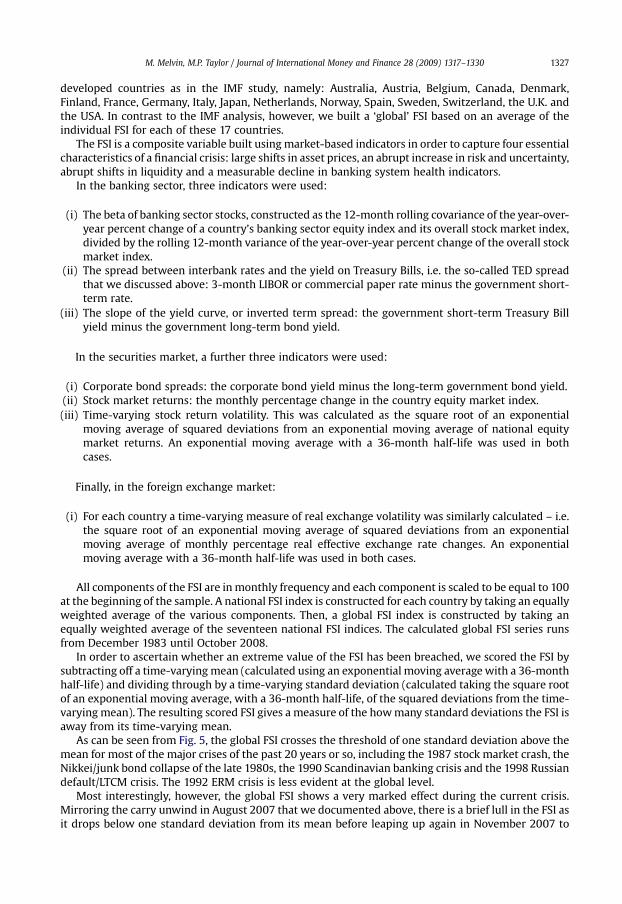
In order to ascertain whether an extreme value of the FSI has been breached, we scored the FSI bysubtracting off a time-varying mean (calculated using an exponential moving average with a 36-monthhalf-life) and dividing through by a time-varying standard deviation (calculated taking the square rootof an exponential moving average, with a 36-month half-life, of the squared deviations from the time-varying mean). The resulting scored FSI gives a measure of the how many standard deviations the FSI isaway from its time-varying mean.

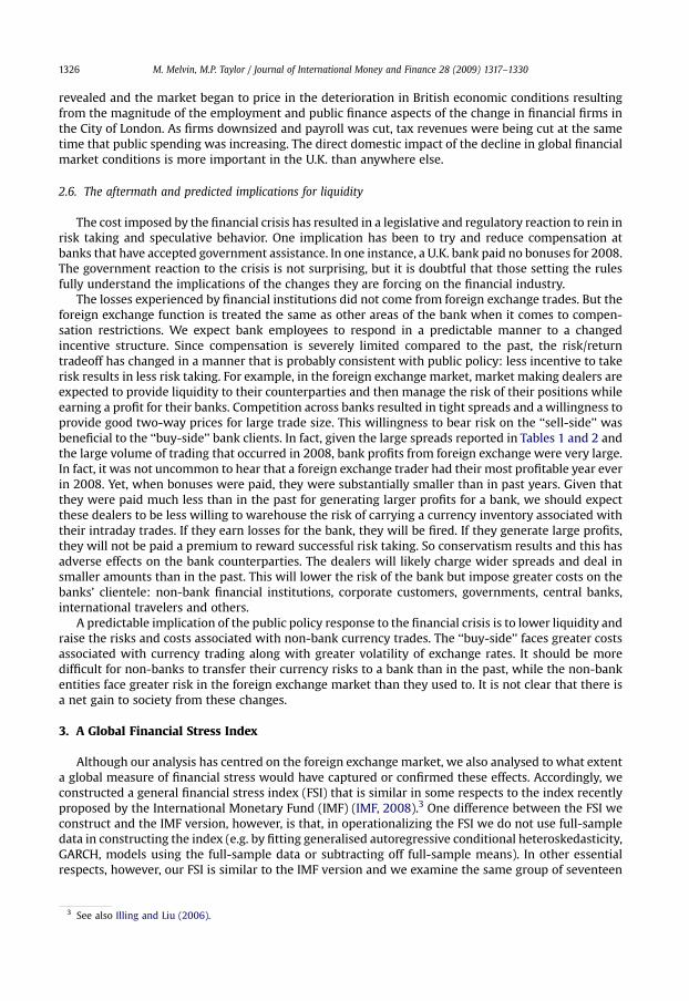
As can be seen from Fig. 5, the global FSI crosses the threshold of one standard deviation above themean for most of the major crises of the past 20 years or so, including the 1987 stock market crash, theNikkei/junk bond collapse of the late 1980s, the 1990 Scandinavian banking crisis and the 1998 Russiandefault/LTCM crisis. The 1992 ERM crisis is less evident at the global level.

Most interestingly, however, the global FSI shows a very marked effect during the current crisis.Mirroring the carry unwind in August 2007 that we documented above, there is a brief lull in the FSI asit drops below one standard deviation from its mean before leaping up again in November 2007 to

-3

-2

-1

0

1

2

3

4

5D

ec-8

3

Dec

-85

Dec

-87

Dec

-89

Dec

-91

Dec

-93

Dec

-95

Dec

-97

Dec

-99

Dec

-01

Dec

-03

Dec

-05

Dec

-07

Fig. 5. Scored Global Financial Stress Index.

M. Melvin, M.P. Taylor / Journal of International Money and Finance 28 (2009) 1317–13301328

nearly 1.5 standard deviations from the mean. The global FSI then breaches the two-standard deviationthreshold in January 2008 and again in March 2008 (coinciding with the near collapse of Bear Stearns).With the single exception of a brief lull in May 2008, when the global FSI falls to about 0.7 standarddeviations above the mean, it then remains more than one standard deviation above the mean for therest of the sample, spiking up in October to more than four standard deviations from the meanfollowing the Lehman Brothers debacle in September.

It is tempting to infer from this analysis that an active currency manager could have significantlydefended their portfolio by taking risk off (or perhaps even going short carry) in August 2007, espe-cially as the carry unwind documented in Fig. 1 is confirmed as a crisis point by the movements in theglobal FSI in the same month. We carried out a first exploration of this idea by estimating a Probitmodel of significant drawdowns from the carry trade investment as a function of the global FSI, wherea ‘‘significant drawdown’’ is defined as greater than a one standard deviation negative return. Table 3presents the estimation results. Clearly, the probability of a major drawdown from a carry tradeinvestment is increasing in the FSI. Table 3 yields evidence of statistical significance of the effect of theFSI on the carry trade.4 What about economic significance?

To examine the economic significance of the FSI effects on carry trade returns, we simulate thereturns an investor would earn from investing in the Deutsche Bank Carry Return Index. Supposethe investor just invests in the index in an unconditional sense, without regard to market condi-tions. We will call this the ‘‘unconditional return.’’ Alternatively, the investor can invest in the indexin ‘‘normal’’ periods and close out the position in stressful periods, where stress is measured by theglobal FSI. Specifically, when the FSI exceeds a value of 1, the carry trade exposure is shut off;otherwise, the investment is held. Fig. 6 illustrates the cumulative returns to such strategies. Thecumulative unconditional return is �1% while the conditional return is þ38% over the periodstudied.

Our carry trade horse race clearly indicates a superior performance of conditioning the carry tradeinvestment on the FSI. In more familiar investment metrics, over the entire 2000–2008 period studied,the unconditional strategy yielded an information ratio (IR, measuring return per unit of risk) equal to�0.03 while the conditional return yields an IR of 0.69. Over the more recent 2005–2008 period, theunconditional IR is �0.66 while the conditional IR is 0.31. In this regard, we see that the FSI as a riskindicator has potential value to FX investments.

4 A consideration of factors that might control carry trade losses is receiving increased attention in the literature lately. Someexamples are Brunnermeir et al, (2008); Jurek (2007); and Clarida et al. (2009).

Table 3Carry trade investment drawdowns and the Financial Stress Index.

Dependent variable: NEGRETMethod: ML – binary Probit (quadratic hill climbing)Sample: 2000M01 2008M10Included observations: 106Convergence achieved after 5 iterationsCovariance matrix computed using second derivatives

Coefficient Std. error z-Statistic Prob.

Constant �1.436662 0.196568 �7.308709 0.0000FSI 0.446948 0.143449 3.115719 0.0018

McFadden R2 0.142782 Mean of dependent variable 0.113208SD of dep. variable 0.318352 SE of regression 0.290921Akaike info criterion 0.643222 Sum of squared residuals 8.802070Schwarz criterion 0.693476 Log likelihood �32.09079Hannan–Quinn criterion 0.663591 Restricted log likelihood �37.43595LR statistic 10.69033 Average log likelihood �0.302743Prob (LR statistic) 0.001077

Obs. with NEGRET ¼ 0 94 Total obs. 106Obs with NEGRET ¼ 1 12

The table reports results of a Probit regression estimation of periods of significant negative returns to an investment in theDeutsche Bank Carry Index as a function of the Financial Stress Index (FSI). A significant drawdown is defined as a greater than 1standard deviation (0.0247) negative return in a month. The results suggest statistically significant effects of greater financialstress in the market increasing the probability of a significant drawdown.

M. Melvin, M.P. Taylor / Journal of International Money and Finance 28 (2009) 1317–1330 1329

Caveats regarding this analysis are as follows:

(1) These results ignore transaction costs. This is important as when the FSI signals significant stress,market conditions are such that we should observe widespread carry trade unwinding. So aninvestor will face large one-sided market conditions that will lead to a much greater than normalcost of trading. Tables 1 and 2 provided indicative information on how much bid-ask spreadswidened in the post-Lehman Brothers period. This is also indicative of what one might expectduring a period of major carry unwind. Furthermore, investors seeking to sell out of their carrypositions will face very thin offers on the other side of their trade. For instance, to close out the

-.1

.0

.1

.2

.3

.4

00 01 02 03 04 05 06 07 08

CONCUMRET CUMRET

Fig. 6. The returns to the carry trade. The graph illustrates the cumulative returns to an investment in the Deutsche Bank CarryIndex. In the unconditional case, the investor simply maintains the investment regardless of market conditions. In the conditionedcase, the investment is shut off when the Global FSI index of financial market risk signals a particularly stressful period.

M. Melvin, M.P. Taylor / Journal of International Money and Finance 28 (2009) 1317–13301330

carry trade strategy of short yen (JPY), long New Zealand dollar (NZD) would involve buying JPYand selling NZD. But if there is great interest to do the same trade across the market, there will bevery little flow interested in selling JPY and buying NZD, so market makers will price tradesaccordingly so that the price of exiting the carry trade will be much higher than in normal times.

(2) These results assume the carry trade exposure is eliminated in the same month that the FSI signalsstress. There may be a lag between recognition of the market stress and exiting the position. If thecarry trade exposure is eliminated in the month following the FSI signal of stress, the IR falls from0.69 to 0.42 over the entire 2000–2008 sample period and from 0.66 to 0.00 over the recent 2005–2008 period. If the investor cannot recognize the shift to the stressful state in real time, it may betoo late in many cases to reduce carry trade exposure.

4. Conclusions

The financial crisis of 2007–? has had major implications for the foreign exchange market. In theearlier part of this paper, we reviewed events and implications for exchange rates, volatility, returns tocurrency investing, and transaction costs. This ‘‘blow-by-blow’’ narrative is intended to be a resourcefor researchers seeking a comprehensive review of the ‘‘what, why and when’’ of the crisis in theforeign exchange market.

The crisis began in August 2007, when subprime-related turmoil in other asset classes finally spilledover into the currency market. This initial phase of the crisis was manifested in a major carry trade sell-off. Then in November 2007, credit restrictions were associated with a major deleveraging in financialmarkets and many investment funds were forced to liquidate positions. The next major wave of thecrisis arrived in March 2008 with the near-failure of Bear Stearns. The treatment of Bear Stearns as ‘‘toobig to fail’’ and the orderly takeover by JP Morgan Chase appeared to calm the market so that somesemblance of normality returned to financial markets. The peak of the crisis (at least, so far) was theSeptember 2008 failure of Lehman Brothers. By any metric, the crisis in the wake of the LehmanBrothers bankruptcy was unlike anything that had preceded this period: volatility reached unseenlevels, liquidity disappeared as counterparty risk reached unprecedented levels so that the cost oftrading currencies skyrocketed and it became very difficult to trade any substantial size.

In the later part of the paper, we developed a financial stress index (FSI) that is an operationalized,global version of the FSI suggested by the IMF, and we then used the global FSI to illustrate the dramaticnature of the current crisis compared to earlier crises. We also examined how the global FSI might havebeen used to condition the exposure to the carry trade (long high interest rate currencies, short lowinterest rate currencies) and we showed that such an index has potential value in protecting a portfolioagainst loss during period of stress, although this result is subject to the important caveats ofcontrolling for transaction costs and timely recognition of the change in regime.

References

Brunnermeir, M., Nagel, S., Pedersen, L., 2008. Carry Trades and Currency Crashes. NBER Macroeconomics Annual, 2008.Cai, J., Cheung, Y., Lee, R., Melvin, M., 2001. Once in a generation yen volatility in 1998: fundamentals, intervention, and order

flow. Journal of International Money & Finance 20, 327–347.Clarida, R., Davis, J., Pedersen, N., 2009. Currency Carry Trade Regimes: Beyond the Fama Regression. Working Paper.Illing, M., Liu, Y., 2006. Measuring financial stress in a developed country: an application to Canada. Journal of Financial Stability

2, 243–265.International Monetary Fund, 2008. Financial Stress and Economic Downturns. World Economic Report, pp. 129–158 (Chapter 4).Jurek, J., 2007. Bendheim Center for Finance. Crash-neutral Currency Carry Trades, Princeton. Working Paper.