The Countywide Truck Travel Demand Model
139
June 2010 www.camsys.com The Countywide Truck Travel Demand Model prepared for Alameda County Congestion Management Agency prepared by Cambridge Systematics, Inc. Dowling & Associates Quality Counts, Inc. final report
Transcript of The Countywide Truck Travel Demand Model

June 2010 www.camsys.com
The Countywide Truck Travel Demand Model
prepared for
Alameda County Congestion Management Agency
prepared by
Cambridge Systematics, Inc.
Dowling & Associates
Quality Counts, Inc.
finalreport


final report
The Countywide Truck Travel Demand Model
prepared for
Alameda County Congestion Management Agency
prepared by
Cambridge Systematics, Inc. 555 12th Street, Suite 1600 Oakland, CA 94607
date
June 2010


The Countywide Truck Travel Demand Model
Cambridge Systematics, Inc. i 8106.001
Table of Contents Executive Summary .................................................................................................. ES-1
1.0 Introduction ......................................................................................................... 1-1 1.1 Overview ...................................................................................................... 1-2
2.0 Review of Existing Truck Model ..................................................................... 2-1 2.1 Existing Truck Model Components ......................................................... 2-2
2.2 Existing Model Validation ......................................................................... 2-3
3.0 Review of Other Truck/Goods Movement Models ...................................... 3-1 3.1 State-of-the-Practice Models ..................................................................... 3-1
3.2 State-of-the-Art Models ............................................................................. 3-6
3.3 Summary of Pros and Cons of Various Modeling Approaches ........... 3-9
4.0 New Truck Modeling Approach ...................................................................... 4-1 4.1 Analysis Framework .................................................................................. 4-1
4.2 Current Truck Model Structure ................................................................ 4-4
4.3 Improvements Made to the Truck Model Structure .............................. 4-4
5.0 Data Collection .................................................................................................... 5-1 5.1 Methods of Counting Trucks .................................................................... 5-1
5.2 New Data Collection .................................................................................. 5-2
5.3 Data Analysis .............................................................................................. 5-9
6.0 Model Development and Validation .............................................................. 6-1 6.1 ODME-Derived trip tables ........................................................................ 6-1
6.2 Trip Generation ........................................................................................... 6-8
6.3 Trip Distribution ....................................................................................... 6-16
6.4 Traffic Assignment ................................................................................... 6-16
7.0 2015 and 2035 Forecasts ...................................................................................... 7-1 7.1 Truck Forecasts ........................................................................................... 7-1
7.2 Port of Oakland Seaport Growth Projections ......................................... 7-8
8.0 Recommendations .............................................................................................. 8-1

Table of Contents, continued
ii Cambridge Systematics, Inc. 8106.001
Appendix A. Arterial Counts ................................................................................... A-1
Appendix B. ACCMA Truck Model Instructions ................................................ B-1
Appendix C. Daily Total Truck Volume Validation – Year 2005 ...................... C-1
Appendix D. Glossary ............................................................................................... D-1

The Countywide Truck Travel Demand Model
Cambridge Systematics, Inc. iii
List of Tables Table ES.1 Existing and New ACCMA Truck Model 2005 Daily Volumes ...... ES-1
Table 2.1 – Existing ACCMA Model Validation Summary Statistics .................... 2-3
Table 5.1 Comparison of Truck Count/Vehicle Classification Methods ........... 5-3
Table 5.2 Highway Count Locations ....................................................................... 5-4
Table 5.3 Arterial Truck Count Locations ............................................................... 5-4
Table 5.4 Conventional (Nonfreeway) State Highway Locations ....................... 5-5
Table 5.5 PeMS Locations .......................................................................................... 5-8
Table 5.6 PeMS Average Daily Traffic Volumes by Subarea and Time Period .......................................................................................................... 5-9
Table 5.7 PeMS Average Daily Traffic Volumes and Percent Change from April 2005 by Individual Location and Time ...................................... 5-11
Table 5.8 Assessment of Highway Truck Traffic Counts ................................... 5-15
Table 5.9 Traffic Count Data at SR 24 .................................................................... 5-16
Table 5.10 Summary of Daily Freeway Traffic and Truck Counts ...................... 5-18
Table 6.1 Observed Count Data by Facility Type* ................................................ 6-5
Table 6.2 Existing Truck Model Validation ............................................................ 6-7
Table 6.3 Existing Truck Model Validation ............................................................ 6-8
Table 6.4 Truck Trip Generation Model Coefficients ............................................ 6-9
Table 6.5 Trip Generation Model Validation Summary ..................................... 6-10
Table 6.6 Port of Oakland Locations ...................................................................... 6-11
Table 6.7 Port of Oakland Locations ...................................................................... 6-13
Table 6.8 Oakland Airport ...................................................................................... 6-14
Table 6.9 Year 2005 Daily Traffic Assignment Validation by Vehicle Class and Facility Type ..................................................................................... 6-24
Table 6.10 Year 2005 AM Peak-Hour Traffic Assignment Validation by Vehicle Class and Facility Type ............................................................. 6-25
Table 6.11 Year 2005 PM Peak-Hour Traffic Assignment Validation by Vehicle Class and Facility Type ............................................................. 6-26
Table 6.12 Year 2005 PM Peak Two Hours Traffic Assignment Validation by Vehicle Class and Facility Type ....................................................... 6-27

List of Tables, continued
iv Cambridge Systematics, Inc.
Table 6.13 Year 2005 PM Peak Four Hours Traffic Assignment Validation by Vehicle Class and Facility Type ....................................................... 6-28
Table 7.1 Year 2015 Traffic Assignment Validation by Vehicle Class and Facility Type ............................................................................................... 7-2
Table 7.2 Year 2035 Traffic Assignment Validation by Vehicle Class and Facility Type ............................................................................................... 7-3
Table 7.3 Compounded Annualized Rate of Growth by Vehicle Type .............. 7-8
Table 7.4 Port of Oakland Containerized Cargo Historical Data ....................... 7-9
Table 7.5 Port of Oakland Containerized Cargo Projected Future Data ............ 7-9

The Countywide Truck Travel Demand Model
Cambridge Systematics, Inc. v
List of Figures Figure 1.1 FHWA 13-Class Vehicle Scheme ............................................................. 1-3
Figure 1.2 Elements of Freight Forecasting .............................................................. 1-5
Figure 3.1 Economic Activity Model Process ........................................................... 3-5
Figure 4.1 FAF Freight and All Trucks Volumes in the East Bay Area ................ 4-3
Figure 6.1 Bay Areawide Count Locations used for ODME-based Trip Tables .......................................................................................................... 6-4
Figure 6.2 Port of Oakland Locations ...................................................................... 6-12
Figure 6.3 Port of Oakland Locations ...................................................................... 6-13
Figure 6.4 Oakland Airport ...................................................................................... 6-15
Figure 6.5 Trip Length Frequency Distribution for IE/EI Small Truck Trips ... 6-17
Figure 6.6 Trip Length Frequency Distribution for IE/EI Medium Truck Trips........................................................................................................... 6-18
Figure 6.7 Trip Length Frequency Distribution for External Combination Truck Trips ............................................................................................... 6-19
Figure 6.8 Trip Length Frequency Distribution for Internal-Internal Small Truck Trips ............................................................................................... 6-20
Figure 6.9 Trip Length Frequency Distribution for Internal-Internal Medium Truck Trips ............................................................................... 6-21
Figure 6.10 Trip Length Frequency Distribution for Internal-Internal Combination Truck Trips ....................................................................... 6-22
Figure 7.1 Truck Forecasts – A.M. Peak Hour – I-80 at University Avenue ........ 7-4
Figure 7.2 Truck Forecasts – A.M. Peak Hour – I-880 near Oakland Airport ..... 7-5
Figure 7.3 Truck Forecasts – A.M. Peak Hour – I-880 at Industrial ...................... 7-6
Figure 7.4 Truck Forecasts – A.M. Peak Hour – Eastern Alameda County ......... 7-7
Figure 7.5 Port of Oakland Containerized Cargo Projected Growth .................. 7-10


The Countywide Truck Travel Demand Model
Cambridge Systematics, Inc. ES-1
Executive Summary Alameda County faces a critical need for forecasting truck impacts. The Port of Oakland and Oakland Airport are the commercial hubs for truck traffic. Alameda County has five of the top 10 most congested corridors in the Bay Area, and each of these corridors is major truck routes.
The current Alameda County Congestion Management Agency (ACCMA) truck model comes from a nearly 20-year old truck model originally developed by the Metropolitan Transportation Commission (MTC). Also, it was not validated with truck counts. Therefore, the current model greatly under-predicts the num-ber of trucks operating on Alameda County roadways. The new model shows a more realistic picture of actual truck travel in Alameda County. The overall improvement of the model in terms of forecasting trucks is shown below in Table ES.1.
Table ES.1 Existing and New ACCMA Truck Model 2005 Daily Volumes
Performance Measure Old Model New Model
Sum of Observed Truck Volumes 321,800 321,800
Sum of Modeled Truck Volumes 139,000 310,400
Percent Error -57% -4%
The truck model project consisted of a number of elements, starting with a review of the existing ACCMA truck model (Chapter 3). The project team, with support from the Model Task Force, also conducted an analysis of peer agency (large county transportation agencies and metropolitan planning organizations (MPO)) truck models (Chapter 4). Armed with an understanding of the existing truck model and informed about the range of potential truck model improve-ments, the set of preferred model enhancements for ACCMA was formulated (Chapter 6) based on available project resources.
New truck traffic counts were collected throughout Alameda County, and off-the-shelf truck traffic data were assembled for the other counties in the model coverage area (the eight other Bay Area counties, plus San Joaquin County) (Chapter 6). The new counts were used for model development and model vali-dation activities (Chapter 7). Also included for this project are future year traffic forecasts for 2015 and 2035 (Chapter 8).
The project also includes recommendations for a next generation ACCMA truck and freight model system. Because the long-distance nature of commercial goods movement, an initial suggestion is to monitor and perhaps partner with MTC and the State of California truck and goods movement model development efforts.

The Countywide Truck Travel Demand Model
ES-2 Cambridge Systematics, Inc.
The Countywide Travel Demand Model Update to Improve Modeling Truck Impacts Project was funded by a California Department of Transportation (Caltrans) Fiscal Year (FY) 2007/2008 Partnership Planning Grant. The new ACCMA truck model now includes a number of new enhancements, including the following:
New truck counts collected at key locations throughout Alameda County. The foundation of any model system lies in the data. For this project, new truck counts were collected at one dozen highway locations and at 50 arterial locations. In addition, Performance Measurement System (PeMS) data were examined throughout Alameda County, with an emphasis on including loca-tions where new data was collected. These data were supplemented with published Caltrans documents.
Updated classifications of trucks that dovetail with truck counts. The existing truck model has a separate classification for very small trucks (vans and pickups). The problem with this classification is separating out vans and pickups used for personal purposes from those used for commercial pur-poses. Therefore, Very Small Trucks classification is not included in the new truck model. The new truck model resolved some of these inconsistencies, although additional research into understanding very small trucks would be a potentially useful future model enhancement. It is important to note, how-ever, that the issue of very small trucks is unresolved across nearly every regional travel model in North America as essential new data collection efforts would be very expensive.
A special truck trip generator for the Port of Oakland Seaport. It was found that the existing truck model underestimated truck trips to the Port of Oakland by 90 percent. A new special generator model was created to more accurately predict truck trips to and from the Port of Oakland. A review of the Oakland Airport area showed the new truck model adequately predicts trucks so an additional special generator was not required.
An innovative and cost-effective approach to estimating observed truck trip generation rates and travel patterns using new truck count data. A key problem with commercial travel (i.e., truck trips) is the lack of knowledge on actual travel patterns. Truck counts provide a snapshot of truck activity at specific locations, but by themselves do not inform where truck trips start and end. In addition, there is no real observed knowledge about truck trip generation rates, or how long each truck trip is in miles or minutes (or hours).
The project team developed an innovative methodology to estimate observed truck trip rates and travel patterns as a cost-effective response given overall project resources and objectives. (This methodology is described in detail in Chapter 7, Section 1). Given observed trip generation and distribution data, the project team was able to develop appropriate models. This methodology

The Countywide Truck Travel Demand Model
Cambridge Systematics, Inc. ES-3
used here was the subject of a paper presented to the Innovations in Travel Modeling Conference held in May 2010 in Tempe, Arizona1.
Separation of short-distance (intraregional) truck trips from long-distance (interregional) truck trips. A key problem with the older version of the truck model was that trucks were not permitted to leave the Bay Area. It is well understood that many trucks travel long distances to out-of-state and out-of-region locations. Thus, the new truck trip tables were split into intraregional and interregional components.
Traffic assignment improvements that accurately reflect differential capaci-ties of trucks and automobiles. The new truck model provides for direct accounting of truck-based congestion through reporting passenger car equivalents (PCEs). PCEs calculate the specific congestion impacts of trucks versus automobiles; whereas, the prior model considered autos and trucks as generic vehicles. PCEs have an important practical application through direct representation of the amount of roadway capacity each type of vehicle consumes. An added feature is the traffic assignment now reports three classes of trucks; whereas, the older version of the model reported total trucks.
Base year model validation and future year forecasts to be used as starting points for upcoming ACCMA studies. The end product of this project was development of base and future year forecasts of Alameda County travel demand for trucks and automobiles. These forecasts, and underlying input data, are ready for use in a variety of applications, ranging from localized traffic studies to the countywide planning analyses.
In all, these enhancements represent a significant upgrade in ACCMA truck modeling capabilities. The following report covers all details of the truck model development efforts.
The overall documentation for this project include this project report, network plots available at the ACCMA web site. The detailed link-level validation results for all count locations and model time periods included in Appendix B is also available in the model DVDs as electronic workbook.
1 http://itm2010.fulton.asu.edu/ocs/index.php/itm/itm2010/index.

The Countywide Truck Travel Demand Model
Cambridge Systematics, Inc. 1-1
1.0 Introduction The objective of the study has been to enhance the ACCMA Travel Demand Model to better forecast truck travel and truck impacts in congested corridors. Although ACCMA has had an existing truck model system, based on the model developed by MTC, it is inadequate for current analytical needs. ACCMA needs to evaluate truck and freight projects the same way it does other roadway and transit projects in the Countywide Transportation Plan (CTP). The Port of Oakland’s sea and airport are regional commerce hubs that have significant transportation impacts. In addition, there are numerous goods movement-related businesses spread throughout the County. MTC’s Regional Goods Movement Study (RGMS) estimated that, in terms of volume, about 80 percent of goods are moved by trucks. There is also a need to model truck activity in con-gested corridors of Alameda County. Alameda County is one of the largest counties in California, and one of its most congested. The County had six of the top 10 most congested corridors in the Bay Area in 2007. The RGMS also deter-mined that I-880 receives the highest amount of truck traffic in the Bay Area, and I-580 is the primary connection between the Bay Area and the national interstate truck network.2
Analysis of freight and goods movement has become a major concern in the transportation community. Our economy depends on the fast and reliable deli-very of goods. In addition, trucks contribute a large amount of vehicle miles of travel (VMT) and emissions to statewide travel. Also, the need for infrastructure improvements to facilitate goods movement far outpaces available funding. Enhanced goods movement and freight modeling systems will be required to address the complex policy questions that confront policy-makers these days throughout the United States.
A Task Force consisting model experts from MTC, Santa Clara Valley Transportation Authority (VTA), and Caltrans, and staff from local agencies (including Alameda-Contra Costa Transit District (AC Transit); Port of Oakland; and Cities of Alameda, Oakland, Fremont, San Leandro, and Livermore) pro-vided guidance throughout the process of truck model development. The Task Force met on a monthly basis throughout the project.
2 Metropolitan Transportation Commission, Regional Goods Movement Study, 2004,
http://www.mtc.ca.gov/planning/rgm/background.htm.
The Countywide Truck Travel Demand Model
1-2 Cambridge Systematics, Inc.
1.1 OVERVIEW The ACCMA Truck Model project included the following tasks. Each of these tasks serves as separate chapters in the body of this report.
Review of state-of-the-practice truck and freight models;
Applicable enhancements to be applied to the ACCMA truck model;
Data needs/data collection;
Truck model development approach;
Model calibration and validation; and
Future year forecasts.
However, before delving into the individual chapters of this report, it is worth-while to examine what the definition of a truck is. A number of schemes have variously been used throughout the nation in terms of a definition of a truck in the development of truck/freight models:
Truck classification schemes;
Number of axles;
Number of units;
Gross vehicle weight rating;
Loaded weight;
Vehicle length; and
The Federal Highway Administration (FHWA) 13-class scheme (see Figure 2.1, below).
After considering the various options above, the project team ultimately settled on the FHWA 13-class scheme as the most logical way of defining and grouping trucks for the ACCMA model, which was consistent with the classification counts gathered for use in validation, and for which crosswalks to groupings for other purposes; for example, gross vehicle weight (GVW) used for emissions analysis are most readily available.

The Countywide Truck Travel Demand Model
Cambridge Systematics, Inc. 1-3
Figure 1.1 FHWA 13-Class Vehicle Scheme
Review of State of the Practice in Truck/Freight Models
The objective of this task was to review the state of the practice of regional and local truck and freight models to identify approaches that may be applicable for the ACCMA model. A number of resource documents were first identified that cover the latest trends in truck and freight forecasting. These resources included:
The National Cooperative Highway Research Program (NCHRP) Report 606, Forecasting Statewide Freight Toolkit;
The NCHRP Synthesis 298, Truck Trip Generation Data;
The Countywide Truck Travel Demand Model
1-4 Cambridge Systematics, Inc.
The 1996 and 2008 editions of the FHWA’s Quick Response Freight Manual (QRFM);
The National Highway Institute’s (NHI) Course 139002 – Freight Forecasting in Transportation Planning; and
The FHWA’s Accounting for Commercial Vehicles in Urban Transportation Models.
The Cambridge Systematics (CS) team (including Dowling & Associates and Quality Counts as subcontractors) also has developed truck and/or freight mod-els for many state departments of transportation (DOT) and MPOs; and has extensive experience with local truck analysis projects. With that experience, a number of truck models were evaluated, including:
Santa Clara VTA Truck Model
Los Angeles County (Metro) Cube Cargo Model;
Southern California Association of Governments (SCAG) heavy-duty truck model;
San Joaquin Valley Goods Movement Study; and
Maricopa Association of Governments (MAG) Truck Model.
Truck and freight modeling techniques can be classified broadly into the fol-lowing eight categories based on objective, methodology, and data requirements:
1. Link-based factoring;
2. Origin-destination (O-D) factoring;
3. Freight truck models;
4. Four-step commodity models;
5. Economic activity models;
6. Hybrid models;
7. Logistics/supply chain models; and
8. Tour-based models.
Given the resources available for this study, the project team decided early on to concentrate on truck model systems. This flow of potential activities is shown in Figure 2.2, below. It was not anticipated that commodity flow forecasting and mode choice models could be developed within the project budget, so efforts were concentrated on trip generation and distribution methods along with traffic assignment.

The Countywide Truck Travel Demand Model
Cambridge Systematics, Inc. 1-5
Figure 1.2 Elements of Freight Forecasting
Economic Forecasting
Commodity Flow Forecasting
Facility Flow Forecasting
Mode Choice
Freight Routing
Trip Generation and Distribution Methods
Multimodal Trip Tables
Networks
Input Data
Modal Trip Tables
Freight Traffic Forecast
Source: NHI Course 139002 – Freight Forecasting in Transportation Planning.
Applicable Enhancements for the ACCMA Truck Model
The tasks identified here were the types of enhancements that would meet the needs of ACCMA, assist ACCMA in reviewing those enhancements, and rec-ommend the improvements that implemented in subsequent tasks.
The CS team met regularly with ACCMA staff and the Model Task Force to cover existing and emerging issues that could be better addressed by an improved truck model. Among the relevant documents considered for this effort included various plans in Alameda County, including the ACCMA Community-Based Transportation Plans; the MTC planning documents, including the Transportation 2030 Plan: Mobility for the Next Generation, draft Transportation 2035 Plan: Change in Motion, and the Regional Goods Movement Study for the San Francisco Bay Area; and transportation planning documents from other agencies to document the truck issues wherein the analysis would be improved by an enhanced ACCMA truck model.
The framework for considering model enhancements was considered according to the framework established in Figure 1.2. An advantage of grouping by model component, as shown in Figure 1.2, is that certain model components (for exam-ple, truck assignment) may be common to many different model types (for example, trip-based or commodity-based).
Ultimately, it was decided that improvements to trip generation, distribution and assignment methods, combined with new roadway data collection efforts, con-stituted the best approach given the limited available resources. Long-term enhancements were also examined, and these are discussed in Chapter 8.

The Countywide Truck Travel Demand Model
1-6 Cambridge Systematics, Inc.
Identify Data Needs and Collect Data
This task included identification of data needs to support the modeling efforts and to collect the identified data. Quality Counts was hired to collect freeway and arterial counts at a number of locations throughout Alameda County.
A number of methods for collecting trucks were considered. In the end, a com-bination of hose counts, manual classification counts, and radar detector units were used (This technology is discussed in more detail in Chapter 5.).
Some issues were encountered during data collection; and Chapter 5 examines how these issues were first identified, and then resolved. In the end, a useful database of functional counts was collected and utilized throughout the model development and, particularly model validation efforts.
Model Development Approach
It is useful to consider travel model systems from a life-cycle perspective. There are four basic stages of a model system: 1) development, 2) validation, 3) application, and 4) maintenance. This project concerns are primarily the development and validation stages; although application and maintenance are critical components and were continuously considered.
The model development began with using innovative origin-destination matrix estimation (ODME) process as a means for creating synthetic truck trip tables, which could be used as observed trip tables for the different truck types. These ODME matrices were used extensively in the model development and validation process, but were not used in the actual trip generation or distribution models.
A number of model development tasks were completed for this project. These included estimating new trip generation and distribution models, and signifi-cantly improving the traffic assignment process to more directly respond to truck traffic impacts. In addition, a new special generator model was developed for the Port of Oakland Seaport.
Travel Model Development
The new truck model system included model calibration and validation efforts. Key features of the new truck model include splitting trip generation and distri-bution models between trips internal to the 10-county model coverage area, and external trips that have either one trip end outside the model coverage area (internal to external or external to internal) or both ends outside the model cov-erage age (through trips).
In addition, traffic assignment was modified to calculate PCEs. PCEs are used to recognize that trucks take up more roadway capacity than do automobiles. Total volumes are also reported.
Future year forecasts were also prepared as part of this project. Forecasts for ACCMA model time periods were prepared for 2015 and 2035.

The Countywide Truck Travel Demand Model
Cambridge Systematics, Inc. 2-1
2.0 Review of Existing Truck Model The existing ACCMA truck model, which is a component of the Alameda coun-tywide travel demand model, was initially developed by the MTC, first in 19973. This model was based on two sources: 1) a truck corridor study model for I-880 conducted by Barton Aschman, and 2) the FHWA’s QRFM.
The Barton-Ashman model was based on a series of truck travel surveys, including a vehicle intercept survey, employer surveys, truck classification counts, and surveys and interviews conducted at the Port of Oakland.
Trip generation estimates productions and attractions for each of the truck types (very small [2-axle, 4 tires]; small [2-axle, 6 tires]; medium [3-axle]; and combo [4-axle +]) separately. The gravity model is used to distribute productions and attractions between zones for each truck type. However, all model steps after trip distribution are performed with the four truck classifications aggregated to total trucks. Therefore, the final loaded network from the travel demand model did not distinguish between truck type and only contained four vehicle types (drive alone, shared ride (2 persons), shared ride (3 or more persons), and truck). The model script was modified to maintain separate truck classes through the assignment stage in order to evaluate the truck model’s performance.
Analyses from previous truck modeling studies4,5 confirm that the ability to accu-rately predict truck volumes in the lighter weight categories, which are mostly standard pickups and vans, is one of the most serious shortcomings in an urban truck model. These trucks are considered “very small” trucks or the FHWA Class 3 vehicles in the current ACCMA truck model. Many of these trucks are used as personal vehicles and thus, are already captured in the ACCMA passen-ger travel model. It is extremely difficult, when conducting vehicle classification counts to distinguish the commercial use vehicles from the personal use vehicles, which fall under the FHWA Class 3. This leads to poor results when validating the truck model for Class 3 vehicles. For this freight model, “very small” trucks
3 Metropolitan Transportation Commission, 1997, Internal Memorandum from Rupinder
Singh to Chuck Purvis, Model Development, Technical Memorandum #43: 1990 Truck Trip Table.
4 Meyer Mohaddes Associates, SCAG Heavy Duty Truck (HDT) Model, prepared for Southern California Association of Governments, 1999.
5 Cambridge Systematics, Inc., SCAG Truck Count Study: Truck Classification System, prepared for Southern California Association of Governments, August 2001.

The Countywide Truck Travel Demand Model
2-2 Cambridge Systematics, Inc.
will be modeled in the passenger travel modeling framework, but excluded from the truck modeling framework.
A basic visual evaluation of assigned total truck trips from the existing model reveal zero truck trips at external stations, as well as underestimated volumes on major truck corridors outside of Alameda. This issue was identified as a key element to be added to the development of the freight model.
2.1 EXISTING TRUCK MODEL COMPONENTS
Trip Generation Models
Trip generation models included in the existing ACCMA model are described here. These equations come from the original Bay Area truck model developed by MTC6. As mentioned above, the MTC truck model itself came from a study conducted in 1990 by Barton Ashman Associates, based on a series of four truck surveys conducted for the I-880 Intermodal Corridor Study. That model includes trip generation models for nongaraged and for garaged trucks7. The equations in the existing ACCMA model are shown below.
Linked Trips (Productions and Attractions)
2 Axle Trips = 0.0324 * Total Employment
3 Axle Trips = 0.0039 * Total Employment
4+ Axle Trips = 0.0073 * Total Employment
Garage-Based Trip Productions
2 Axle Trips = 0.011 * Manufacturing Employment + 0.014 * Retail Employment + 0.0105 * Service Employment + 0.046 * (Other Employment + Wholesale Employment + Agricultural Employment
3 Axle Trips = 0.014 * Manufacturing Employment + 0.012 * Retail Employment 0.0037 * (Other Employment + Wholesale Employment + Agricultural Employment
4+ Axle Trips = 0.0044 * Manufacturing Employment + 0.0027 * Retail Employment 0.0084 * (Other Employment + Wholesale Employment + Agricultural Employment
6 Ibid 1.
7 Garage trips go back and forth between their base location and delivery/customer locations; lined trips make intermediate stops before returning to their home base.

The Countywide Truck Travel Demand Model
Cambridge Systematics, Inc. 2-3
Garage-Based Trip Attractions
2 Axle Trips = 0.234 * Total Employment
3 Axle Trips = 0.0046 * Total Employment
4+ Axle Trips = 0.0136 * Total Employment
Trip Distribution
Trip distribution is from the MTC model for four truck classes: very small, small, medium, and large trucks. Truck trip tables were created used standard gravity models for truck trips solely within the model coverage area.
Traffic Assignment
For traffic assignment, the four truck classes are summarized into one truck trip category. Total vehicles are assigned, so there is no method for accounting that trucks take up more roadway capacity than automobiles.
2.2 EXISTING MODEL VALIDATION The results of the existing 2005 ACCMA model’s daily assigned trips were com-pared to the observed counts. It should be noted that the validation statistics reported here are only for roadways in Alameda County. Table 2.1 provides validation statistics for the overall model and by vehicle class. As expected, the assigned total vehicles and auto trips meet the acceptable target for percent Root Mean-Square Error (RMSE).
Table 2.1 – Existing ACCMA Model Validation Summary Statistics
Performance Measure Total
Vehicles Autos Total
Trucks Small
Trucks Medium Trucks
Combo Trucks
Sum of Observed Volumes 3,406,000 3,084,000 322,000 70,000 77,000 176,000
Sum of Modeled Volumes 2,993,000 2,732,000 139,000 5,000 25,000 179,000
Percent Error -12% -11% -57% -92% -67% -38%
Percent RMSE 41% 38% 147% 132% 164% 164%
R-squared 0.88


The Countywide Truck Travel Demand Model
Cambridge Systematics, Inc. 3-1
3.0 Review of Other Truck/Goods Movement Models Prior to developing the modeling framework for the new ACCMA model, it is useful to review existing literature on freight and truck travel modeling. This reveals conceptual frameworks that may be useful in the current effort, as well as pitfalls that should be avoided. In the recent past, CS conducted extensive reviews of both the state-of-the-practice and the state-of-the-art modeling tech-niques as part of another study8. The ensuing sections provide a brief description of the various techniques identified in those reviews.
The modeling techniques can be classified broadly into the following eight cate-gories based on objective, methodology, and data requirements:
1. Link-based factoring techniques;
2. Origin-destination (O-D) factoring;
3. Three-step freight truck models;
4. Four-step commodity flow models;
5. Economic activity models;
6. Hybrid models;
7. Logistics/supply chain models; and
8. Tour-based models.
3.1 STATE-OF-THE-PRACTICE MODELS
Link-Based Factoring Techniques
Link-based factoring techniques begin with existing truck volumes on a facility, on a modal network link, or at a freight-related terminal. Factors are developed to estimate changes in truck volumes due to changes in transportation service on the facility or on an alternative facility of the same or different mode. For exam-ple, to develop truck counts in a future year, observed truck counts on a specific highway are increased by three percent per year. The three-percent value may
8 Fischer, M. J., M. L. Outwater, L. L. Cheng, D. N. Ahanotu, and R. Calix, Cambridge
Systematics, Inc., An Innovative Framework for Modeling Freight Transportation in Los Angeles County, prepared for Los Angeles County Metropolitan Transportation Authority, January 2005.

The Countywide Truck Travel Demand Model
3-2 Cambridge Systematics, Inc.
be derived from historical truck volume growth, or based on another surrogate variable such as employment or economic growth. This simplified method per-mits existing data to be applied rapidly, and is usually intended for short-term forecasts. Many assumptions are needed to make these methods work, and the range of applicability is limited. The QRFM, developed for the FHWA, describes methods of applying growth factors to traffic volumes that are applicable to urban highways. Only two model components are required for the simplified method: 1) observed link traffic volumes, and 2) methods to factor these flows.
Origin-Destination Factoring
Origin-Destination (O-D) factoring forecasts truck flows by factoring a base year truck O-D table of truck flows and assigning the new truck O-D tables to the highway network. This method differs from the link-based method; in that, truck volumes are not directly observed, but produced by assigning a truck O-D table to a highway network. A variation on this approach is the factoring of commodity flow tables that provide tonnage flows by commodity between ori-gins and destinations, splitting these flows among the available modes (using a mode choice model or fixed modal shares from the base year), and converting the truck flows to truck trips. The commodity O-D factoring approach is fre-quently used for statewide freight models, which generally focus on long-haul freight movement. Long-haul movement is well characterized in commodity flow datasets, such as the Commodity Flow Survey9 and the Global Insight (for-merly known as Reebie) TRANSEARCH database10.
Three model components are required for the O-D factoring forecast method: 1) a base year O-D trip table for trucks (or a commodity flow table), 2) growth factors for the table, and 3) methods to assign the truck table to the highway network. The growth factors can be based on economic output, employment, or other growth indicators at the zonal level. The growth rates are often developed by using simple economic models. They are then applied to the base year O-D truck trip tables using iterative proportional fitting techniques to balance pro-duction and attraction growth rates. The iterative proportional fitting technique commonly used in transportation planning is known as Fratar factoring. Soft-ware to implement this technique is usually available in travel demand model packages (CUBE, TRANPLAN, TP+, EMME/2, and TransCAD). Methods to
9 The Commodity Flow Survey is a survey conducted by the U.S. Bureau of the Census
every five years based on a survey of establishments. The resulting database provides commodity flows at the national, state, and metropolitan level. Commodity flows are reported in tons, ton-miles, and value, and by mode.
10 TRANSEARCH is a proprietary commodity flow database that provides information on tons moved by mode. O-D information is provided at the county level. Reebie Associates originally developed TRANSEARCH, and the database is often called Reebie data. Reebie Associates was acquired by Global Insights in 2006.

The Countywide Truck Travel Demand Model
Cambridge Systematics, Inc. 3-3
assign truck tables to the highway network depend on the availability of other data and are not limited by the O-D factoring models.
Base year O-D truck trip tables can be estimated in a variety of ways, depending on the availability of data. One approach that has been used with some success is the ODME process. This method utilizes observed truck counts and partial O-D data (usually from O-D surveys) to estimate a truck trip table. Nonlinear programming techniques are used to estimate a trip table that, when assigned to the network, minimizes the difference between predicted and observed truck volumes. The partial O-D data and best judgment estimates for the unknown O-D information are used to construct a “seed” table. The nonlinear program-ming process then adjusts the trip table to obtain the best fit with the truck count data. The base year table produced from the ODME method can then be factored to a forecast year using the methods described previously. ODME models for trucks have been developed in the New York City region by List and Turnquist.11 The ODME process is available as a standard module in the CUBE and TransCAD travel demand model packages.
Three-Step Freight Truck Models
Freight truck models develop highway freight truck flows by assigning an O-D table of freight truck flows to a highway network. This is the class of truck model currently included in the ACCMA travel demand model. The O-D truck table is produced by applying truck trip generation and distribution steps to existing and forecast employment and/or other variables of economic activity for analysis zones. This method differs from O-D factoring; in that, the O-D table is estimated directly using trip generation rates/equations and trip distribution models at the traffic analysis zone (TAZ) level. The mode choice step is unneces-sary since truck trips are estimated directly, and there is no need for the consid-eration of other possible modes for moving freight. The components required for this modeling technique include existing and forecast zonal employment data, methods to generate zonal freight productions and attractions by using truck trip generation rates, methods to generate truck O-D flows by applying trip distribu-tion procedures to truck productions and attractions, and methods to assign the O-D freight truck flows to a highway network.
Freight truck models usually attempt to account for shipment of goods, including local delivery. Because these models are focused exclusively on the truck mode, they cannot analyze shifts between modes. Truck models are usually part of a comprehensive model that forecasts both passenger and freight movement, and consequently will often use a simultaneous assignment of truck trips with auto trips.
11List, George F., and Mark A. Turnquist, 1995, “Estimating Truck Travel Patterns in
Urban Areas,” Transportation Research Record 1430.

The Countywide Truck Travel Demand Model
3-4 Cambridge Systematics, Inc.
As noted above, freight truck models follow a three-step process of trip genera-tion, trip distribution, and traffic assignment. Trip generation estimates the number of trips either produced in each zone or attracted to each zone; and is usually a function of socioeconomic characteristics of the zone (employment by industry, population, or number of households). Trip generation is accom-plished using truck production and attraction equations, whose coefficients are estimated based on local commercial vehicle surveys or by using parameters bor-rowed from other sources such as the QRFM. Trip distribution determines the connection between trip origins and trip destinations. Trip distribution is gener-ally accomplished using a gravity model similar to that used in a passenger model. In the gravity model, the number of trips that travel between one zone and another is a function of the number of trip attractions in the destination zone, and is inversely proportional to a factor measuring the impedance between the two zones. (The gravity model is usually related to the travel time between two zones (i.e., the longer it takes to get from one zone to another, the less attrac-tive trips to that destination zone become).) Parameters in the gravity model can be developed from local surveys or borrowed from other sources, such as the QRFM. The route that trucks use to get from origin to destination is a function of network characteristics, taking into account traffic conditions on each route. Network assignment of the truck trips is usually based on a multiclass equili-brium highway assignment that includes passenger cars; in other words, the model looks for the shortest time path for all trips simultaneously. Freight truck models can take into account the different classes of trucks and their impact on congestion compared to automobiles (large trucks cause more congestion because they occupy more space than autos). In addition, the networks can be coded so that any specific link can either allow only truck trips, or can exclude the use of truck trips.
Four-Step Commodity Flow Models
The four-step commodity flow model is similar in structure to the four-step pas-senger model. Both the four-step commodity flow models and the four-step pas-senger models require the development of a network and zone structure. Since a larger percentage of freight trips in an urban area are long haul than is the per-centage of passenger trips that are long haul, a skeletal highway network exter-nal to the region is usually appended to a local passenger network to allow for assignment of these long-haul freight trips. Commodity models can analyze the impact of changes in employment, trip patterns, and network infrastructure.
The commodity-based “trip” generation model actually estimates the tonnage flows between origins and destinations. These flows are converted to vehicle trips after the mode choice step in the process. The trip generation models include a set of annual or daily commodity tonnage generation rates or equations by commodity group that estimate annual or daily flows as functions of TAZ, or county population and disaggregated employment data. Base year commodity flow data at the zonal level are used to estimate the trip rates or trip generation equations. The O-D tables for these flows are typically estimated using gravity

The Countywide Truck Travel Demand Model
Cambridge Systematics, Inc. 3-5
models similar to the trip distribution step in four-step passenger models. Trip distribution models are estimated separately for each different commodity group. The unit of flow in the O-D table is typically tons shipped. The distribu-tion of freight is to a national system of zones, recognizing the large average trip lengths in this class of models. Mode split is a necessary component because O-D patterns are developed for particular commodities rather than for trucks. Quite often, the mode split step simply assumes that the base year mode share of each commodity flow stays the same in the future. The conversion of commodity truck tonnage to daily freight truck trips uses the application of payload factors (average weight of cargo carried per vehicle load). Payload factors can be esti-mated on a commodity-by-commodity basis using locally collected survey data (e.g., roadside intercept surveys) or national surveys (e.g., the U.S. Census Bureau Vehicle Inventory and Use Survey). The assignment of truck freight will typically use either a freight truck only or multiclass assignment model.
Economic Activity Models
An economic activity model includes an economic or land use model as a step before the traditional four steps. Economic activity models are the freight equiv-alent of the integrated land use transportation models used in the analysis of urban passenger travel. They require specific data concerning the availability of land and the rules governing the development and location of certain industries, and an understanding of the interdependencies between industries.
Economic activity models estimate the flows of commodities between economic sectors and between zones. They assume that the zonal employment or eco-nomic activity is not directly supplied to the model, but is created by applying an economic or land use model. The modeling technique used for economic activity models is known as a spatial input-output (I-O) model. The spatial I-O model distributes household and economic activity across zones, uses links and nodes of a transportation network to connect the zones and model the transportation system, and then calculates transportation flows on the network. It uses a land use component to generate and distribute trips and a transportation component to generate mode split and network assignments. The two sides of the model inform each other, resulting in a dynamic model, as shown in Figure 3.1.
Figure 3.1 Economic Activity Model Process
Economy and Land Use
Structure of the economy
Location of the activity
Transportation Component
Network Mode Split
Costs
Trip Generation
Distribution
The model uses an I-O structure of the economy to simulate economic transac-tions that generate transportation activity. A spatial I-O model identifies

The Countywide Truck Travel Demand Model
3-6 Cambridge Systematics, Inc.
economic relationships between industries and between industries and households, accounting for the geographic or spatial relationships associated with the economic relationships (origins and destinations of the economic flows). In future years, the spatial allocation of economic activity, and thus trip flows, is influenced by the attributes of the transport network in previous years. Thus, the model is dynamic with respect to land use and transportation. The economic activity model differs from the four-step commodity class of models as it uses an economic or land use model to forecast zonal employment or economic activity prior to the trip generation step. The freight component of the Oregon DOT’s statewide travel demand model is an example of an economic activity model.
Hybrid Models
State-of-the-practice metropolitan truck models are hybrids that blend commod-ity flow modeling techniques with freight truck modeling techniques. Com-modity flow databases tend to be relatively accurate for intercounty flows, but undercount intracounty flows because commodity flow databases rely in part on economic input-output data that ultimately are based on financial transactions between producers and consumers of goods. However, in an urban area many truck moves are not easily traced to such transactions. Moves from warehouses and distribution centers, repositioning of fleets, drayage moves, parcel delivery, and the like are generally short-distance trips in which there may not be an eco-nomic exchange of the goods from one party to another. To compensate for the undercounting of the shorter distance trips, local truck trips are generated based on local employment and economic factors using trip generation rates. These trips are usually generated at the zone level, and trip distribution uses methods such as gravity models. The trip rates are calibrated so that the truck traffic volumes that are generated from the combined commodity flow and locally-generated truck trips match those from available truck counts. Several terms are used to refer to these two trip types, including commodity flow trips versus locally generated trips, external versus internal truck trips, and long haul versus local truck trips.
Hybrid models most often forecast Internal-Internal truck trips through the use of a simple truck model, as shown in the three step truck model described above; and forecast the trucks with at least one external trip end (External-Internal, Internal-External, and External-External) through the use of a commodity process. The forecasting of the external trips may be through importing and factoring a commodity flow survey (e.g., SCAG), or by using a commodity flow survey to develop external model equations (e.g., MAG in Phoenix, Houston-Galveston Area Council (HGAC) in Houston).
3.2 STATE-OF-THE-ART MODELS Research programs throughout North America and Europe are presently devel-oping a new generation of freight models. Two techniques in particular are

The Countywide Truck Travel Demand Model
Cambridge Systematics, Inc. 3-7
receiving widespread interest: 1) logistics/supply chain models, and 2) tour-based models. The logistics/supply chain models borrow techniques from industrial supply chain planning in an effort to track goods as they move along the supply chain from producer to consumer. The tour-based models focus on the trip chain characteristics of intra-metropolitan trucks. Examples of these model types are presented below.
Logistics/Supply Chain Models
GoodTrip Model12
The GoodTrip model combines features of logistics chain models and tour-based models to analyze urban goods movement flows. The model defines a set of activity types, which when linked together may describe either a logistical chain or a set of stops on a vehicle tour (or in some cases, a combination of both). Activity types include:
Consumers,
Supermarkets,
Teleshop,
Hypermarkets,
Urban distribution centers, and
Factories.
The model starts its calculations at the consumption end of the chain, and esti-mates the demand for goods by goods type (analogous to commodity) for each zone in the model. The share of this demand allocated to each of the activity types in each zone is also estimated based on models developed from survey data. The model then uses information about the spatial and functional relation-ships of each of the activity types and probabilities to estimate flows by activity type and zone. The goods flows are then assigned to vehicle tours for each origin-destination pair. The origin’s activity type determines the transport mode, vehicle capacity, vehicle loading factor, and number of stops per tour. This conversion of goods flows to vehicle tours establishes the trip table for assignment to a network.
This modeling approach is of particular interest because of its urban focus and its ability to analyze how changes in logistics organization affect vehicle traffic.
12 Boerkamps and van Binsbergen, “GoodTrip – A New Approach for Modeling and
Evaluation of Urban Goods Distribution,” Delft University of Technology, and The Netherlands Research School for Transport, Infrastructure and Logistics.

The Countywide Truck Travel Demand Model
3-8 Cambridge Systematics, Inc.
SMILE13
Researchers at the Transport Research Centre of the Netherlands Ministry of Transport, Netherlands Economic Institute, and TNO Inro have developed a logistics chain model called Strategic Model for Integrated Logistics Evaluation (SMILE) that can be used as a decision support system for freight transportation policy evaluations. This model begins with an economic input-output modeling approach that calculates supply and demand for each economic sector based on industry production functions. This establishes the economic trade flows for the region of interest. The logistics module assigns each goods flow to a logistics family with common characteristics. The assignment of goods to logistics fami-lies is based on the spatial patterns of supply and demand options for the good. The common characteristics for each logistics family are those that define the type of inventory control and logistics system that will be used to distribute the product. A series of logistics models are developed that define the distribution systems that are used by each logistics family and the spatial organization of warehousing and distribution systems for product delivery and supply chain management. The information about logistics chains is then fed into a transport model that determines the modes of transport used and the optimum modal network paths from origins to destinations.
Tour-Based Models
University of Calgary14
Researchers at the University of Calgary have developed an approach that applies tour-based microsimulation modeling concepts to urban goods move-ment modeling, which was originally developed for passenger modeling. However, in their approach, they define the tours for vehicles rather than for passengers. The model recognizes that many commercial vehicles conduct activities in tours – that is, a series of linked trips that do not necessarily involve a return to home base on every trip. In the model, a synthetic population of business establishments is developed from aggregate data, and these are used to estimate the number of tours generated for a particular commercial activity. The business establishments are the operators of the vehicles that conduct the tours and the approach can be applied to retail establishments, service businesses, or any other type of commercial vehicle operation.
13 Tavasszy, Smeenk, and Ruijgrok, “A DSS for Modeling Logistics Chains in Freight
Transport Policy Analysis,” Seventh International Conference of IFORS, 1997.
14 Hunt, Stefan, and Abraham, “Modeling Retail and Service Delivery Commercial Movement Choice Behaviour in Calgary,” Tenth International Conference on Travel Behaviour Research, 2003.

The Countywide Truck Travel Demand Model
Cambridge Systematics, Inc. 3-9
Stops on the tours are generated based on traditional variables used in trip gen-eration (population, households, employment by business sector). For each vehicle tour, a series of choice models are employed in order to determine the type of vehicle that will be used to conduct the business of the tour, the purpose of each stop (goods pickup or delivery, service, return to home), and the location of the next stop. The choice models are logit choice models that use variables related to what has happened previously on the tour, the attractiveness of zones that could include the next stop on the tour (measured in terms of the number of trip attractions estimated for the zone), and the location of the stops relative to home base (taking into account travel times from zone to zone). The choice models are estimated from travel diary data and have been applied successfully to simulate retail and service trips.
3.3 SUMMARY OF PROS AND CONS OF VARIOUS MODELING APPROACHES Each of the modeling techniques described in the previous sections has strengths and weaknesses. The state-of-the-art-practice commodity flow models have the advantage of being based on extensive and readily-available multimodal freight flow and economic activity data. On the other hand, many local truck moves, including trips from warehouses and distribution centers, fleet repositioning, empty return trips and truck drayage moves, as well as service, utility, and con-struction trucks, are not accounted for in these models. Many of these missed truck trips are short trips within urban areas. Therefore, truck models based exclusively on commodity flow data tend to underestimate truck trips in the urban area. In addition, the commodity flow data are generally not available at the TAZ level, and techniques of questionable accuracy must be used to disag-gregate county-level data.
Models built exclusively from truck trip generation and attraction rates based on local economic activity have the advantage of being tailored to the economic activity data of the study area. Truck trip generation rates can be estimated from local data that include all truck moves, not simply moves based on commodity flows. These models can be made more responsive to changes in local economic activity and population relative to truck models based on commodity flow data. However, truck models based on locally-generated truck trips do not incorporate goods movement factors for external regions. Therefore, external and through truck trips are not well modeled. In addition, changes in external regions over time cannot easily be incorporated into truck model forecasts. The behavioral basis of these models is crude; they cannot reflect changes in the structure of truck operations over time, and they do not accurately account for the trip chain characteristics of many urban truck trips. Finally, the data required to estimate accurate trip generation and distribution models given the variety of truck trip types are very extensive. Collecting sufficient data of this type from private businesses has proven to be very difficult in past studies.

The Countywide Truck Travel Demand Model
3-10 Cambridge Systematics, Inc.
Hybrid models, which take advantage of the benefits of the commodity flow and local truck models, including freight and other non freight truck purposes, have proven to be the most effective modeling framework to date. Long-haul truck trips are modeled using the commodity flow database, which can be adjusted over time based on economic factors. Short-distance truck trips can be estimated as a function of local employment characteristics. The hybrid models are used in several metropolitan areas, and therefore have a theoretical framework that has proven applicable to metropolitan and regional models.
Despite their proven benefits and usefulness, hybrid models lack the ability to fully track logistics chains that have mixed long-haul and local components. The commodity flow data accurately estimate primary movements – that is, the flow from producers to consumers. The extensive information available on the amount of goods produced and consumed in the economy and the location of production and consumption sites help ensure the accuracy of primary com-modity flow data. However, not all of the secondary moves – the intermediate handling of goods at warehouses, distribution centers, and truck terminals – are effectively captured in commodity flow data. Sources such as the Bureau of Transportation Statistics/Bureau of Census Commodity Flow Survey, which surveys warehouses about commodity moves, do not distinguish primary and secondary flows. It is, therefore, impossible to associate these secondary flows with warehouse locations or warehouse activities. The hybrid models attempt to fill this gap by estimating all local truck trips through three-step trip generation and distribution models. However, these models lack explicit links between the primary flows generated by the commodity flow data and the local truck trips. It is impossible to track flows of goods throughout the entire logistics chain to ensure consistency of the two approaches. The hybrid models do not allow for analysis of how changes in logistics patterns affect transportation demand.
Another disadvantage of the hybrid model is that it does not account for the trip-chaining characteristics associated with several different types of local truck moves. Both the commodity flow truck trips and the local truck trips are gener-ated based on a trip being a single origin with a single destination. However, several types of trips (particularly those made within the metropolitan area) are by trucks that utilize a “sequentially unloading, return empty” truck trip pattern. Trucks leave their origins with a full load, make several stops to deliver partial loads, and return empty to their point of origin. Some trucks follow the reverse pattern, leaving their origin empty and returning with a full load after making pickups at multiple locations. These truck trip types are not well captured by the hybrid model. Service trucks also exhibit this trip chaining characteristic.
For the ACCMA truck model improvement project, a commodity flow survey was not available to use as a direct import, or to serve as the basis for the devel-opment of commodity based external trip equations. The inclusion of external truck trips, without the use of commodity trucks, using the Santa Clara VTA methods is discussed in Chapter 6.

The Countywide Truck Travel Demand Model
Cambridge Systematics, Inc. 4-1
4.0 New Truck Modeling Approach This chapter examines important issues that were considered for developing the truck modeling approach for ACCMA. This chapter also discusses enhance-ments to the ACCMA truck model included in this approach. The analysis framework and set of model improvements were selected in consultation with the Model Task Force (MTF).
4.1 ANALYSIS FRAMEWORK In planning for the development of the new truck model system, key considera-tions were evaluated. Those included the following:
Input Data. Some of the truck forecasting methods require data that might not be readily available to ACCMA. Our review examined the availability of base year and forecast employment information.
Performance Outputs. The units of performance of the various forecasting methods vary in terms of the units of flow, the facilities included, the time period covered, and the types of vehicles provided. We understand that ACCMA needs to analyze volumes and speeds of different types of trucks and made sure outputs of forecasting methods were not inconsistent with those needs.
Calibration and Validation Data. The methods need to produce data, which is adjusted to reflect local conditions. Our review indicated what data was needed to calibrate the parameters of the methods (for example truck sur-veys); and what data is needed to validate the link volume forecasts (for example, truck classification counts).
Geographic Scale. The extent and detail of the forecasting methods may vary considerably. Freight trucks may travel hundreds of miles and the geo-graphic coverage needed to address those issues may be inappropriate for ACCMA’s needs. Although the ACCMA model coverage area is extensive – it covers the entire nine-county San Francisco Bay Area plus San Joaquin County – freight and goods movement model coverage areas often include entire states, or the entire United States, plus Canada and Mexico.
Integration with other Models. The ACCMA truck model will not exist in a vacuum. It does need to be consistent and share information with the MTC truck model.
Ease of Use. The methods reviewed vary considerably in the data, man-power, and computer resources required; the updating and maintenance

The Countywide Truck Travel Demand Model
4-2 Cambridge Systematics, Inc.
required; and the schedule time required to complete a forecast. The resources of any method must be judged against the availability of those resources for ACCMA.
An issue which we believe is overarching and relevant to the review is an under-standing that all trucks are included in these forecasting methods. While it is true that all freight on the highway moves in trucks, it is not true that all trucks carry freight. As defined by the organizations concerned with evaluating and forecasting freight, freight trucks typically do not include trucks carrying con-struction material or equipment, service, and utility trucks; and may not include trucks delivery goods locally to retail, commercial, or residential buildings. As shown in Figure 4.1 from the FHWA’s Freight Analysis Framework (FAF), the estimates of freight trucks are concentrated on the major interstates and principal arterials. The FAF acknowledges that those freight truck flows are a small per-centage of the truck flows on other highways in Alameda County and the East Bay area. In fact, according to the FAF2 Highway Link and Truck Data and Documentation: 2002 and 2035, the freight truck VMT in Alameda County represents only 25 percent of the total truck VMT on the roads included in the FAF2 network15.
We estimate that much of the nonfreight truck volumes will grow at a rate in accordance with freight trucks, and understanding freight truck volumes is important to understanding the flow of all trucks; however, methods that provide forecast only of freight trucks may be inadequate for ACCMA’s needs. For ACCMA’s purposes, understanding all truck travel and not just freight-related truck movements is important.
15 FAF and FAF2 technical documentation is available from FHWA at
http://ops.fhwa.dot.gov/freight/freight_analysis/faf/faf2_tech_document.htm.

The Countywide Truck Travel Demand Model
Cambridge Systematics, Inc. 4-3
Figure 4.1 FAF Freight and All Trucks Volumes in the East Bay Area
Source: Cambridge Systematics from FAF2 Highway Link and Truck Data: 2002.

The Countywide Truck Travel Demand Model
4-4 Cambridge Systematics, Inc.
4.2 CURRENT TRUCK MODEL STRUCTURE The current ACCMA model truck trip generation models use the six employ-ment categories contained in the Association of Bay Area Governments (ABAG) socioeconomic database. These employment categories are:
1. Retail
2. Service
3. Other
4. Wholesale
5. Agricultural
6. Other employment groups
In terms of vehicle class for trucks, the original ACCMA model divided trucks into four vehicle classes:
1. Very small trucks. Two-axle, four tires;
2. Small trucks. Two-axle, six tires;
3. Medium trucks. Three-axle; and
4. Combo. Four-axle+.
For traffic assignment, trucks are grouped into a single category. Four vehicle classes are currently included in traffic assignment: drive alone vehicles, shared ride two person carpools, shared rider three or more person carpools, and trucks. Total vehicles are included in the volume-delay function.
4.3 IMPROVEMENTS MADE TO THE TRUCK MODEL STRUCTURE A number of improvements have been made to the ACCMA truck model system. These improvements are introduced here in this section, and applications are described in Chapter 7.
Trip Generation Model
Socioeconomic Data
The socioeconomic data that is typically used to estimate internal trip generation in a truck model is more detailed than those data being used in the auto passen-ger model. Ideally, the employment data should be stratified into more employment categories. This process would provide more accuracy for truck travel, and allows for a direct relationship between the industrial sectors being represented in the internal trip model and the allocation of trucks generated from these industries to TAZs within the region.

The Countywide Truck Travel Demand Model
Cambridge Systematics, Inc. 4-5
At the beginning of the project, the lack of sufficient detail in the employment data was identified as a drawback. Truck trip generation should typically be land use based or industry based, and not occupation based as it is right now. Therefore, a truck model that uses more detailed employment data, such as the North American Industry Classification System (NAICS) 2-digit employment, was proposed. However, upon further research and discussions CS had with MTC and ABAG, it was learned that NAICS 2-digit employment data does not exist for the base year at the TAZ zone level, and cannot be projected to future years. Therefore, it was decided that the current model structure must be retained until new detailed employment data can be obtained.
Truck Trip Rate Calibration
Truck trip generation models use economic variables to forecast truck flows to and from a geographic area using equations. These trip generation equations are typically developed using the truck travel information obtained through truck travel surveys. As recent surveys are not available, the ODME-based truck trip table will be used as an observed data source for validating the truck trip gener-ation model. (Please refer to Chapter 6 for a more detailed description of the ODME process.) The outcome of trip generation is the number of vehicles that comes into or goes from a TAZ in a specified unit of time.
The current truck trip generation rates (or equations) are used to determine the daily truck flows originating or terminating in TAZs as a function of zonal industry sector employment data. In other words, employment data are the essential input data required for computing truck trip generation. These independent variables, such as different types of employment, dictate the level of detail the truck flows can be generated using the trip generation model.
The current trip rates were calibrated based on truck assignment results where the truck model volumes was compared against the truck table developed by counts from ODME by truck type.
Since the TAZ-level employment data is available for only six categories – manu-facturing, retail, service, wholesale, agriculture, and other – the new model will estimate truck trip estimates using only these six categories of land uses/sectors. These new trip rates are separate for production and attraction models, and are described in detail in Chapter 6.
Very Small Trucks
In the new truck model, Class 3 vehicles are not included; however, this vehicle class is included in the passenger model16. Therefore, the three truck types that
16 Truck modeling studies conducted for SCAG confirm that the ability to accurately
predict truck volumes in the lighter weight categories is one of the most serious shortcomings in an urban truck model. Trucks less than 10,000 pounds are considered
Footnote continued

The Countywide Truck Travel Demand Model
4-6 Cambridge Systematics, Inc.
will be part of the new improved truck model are: Class 5 (two-axle, six tires); Class 6 (three-axle, single units); and Classes 7 through 13 (combo units). Please refer back to Figure 1.1.
Since the original ACCMA passenger model keeps truck types separate for trip generation and trip distribution, no changes were made to these steps of the model to modify truck types. For all steps after trip distribution, two sets of changes were made to the Cube script:
1. Very small trucks were not included in the aggregated one truck type (i.e., Truck = Small trucks + medium trucks + combo trucks); and
2. Very small trucks, small trucks, medium trucks, and combo trucks were con-sidered and outputted separately throughout the entire modeling process.
Special Generators
Special generators are those facilities that do not share the same economic rela-tionships as other TAZs in the region. That is, these facilities will either have to be modeled separately based on more local and survey data, or existing traffic counts can be used to account for truck trips originating and ending at various special generators in the region. In the Bay Area, truck vehicle traffic has the greatest impact on Alameda County, as this County contains both the Port of Oakland and Oakland Airport, which is the primary air cargo airport in the Bay Area. Accordingly, the new model will include a Seaport Model as a special generator. In the new improved model, truck counts at the Port of Oakland Seaport will serve as the primary sources of truck trip generation data. For forecast years, growth factors will be applied to these two facilities to produce forecast year truck trip estimates.
The approach to application of the Port of Oakland special generator model was first described by Santa Clara VTA staff in a 2008 Transportation Research Board (TRB) paper. The issue at the Port of Oakland is the trip-based truck trip genera-tion rates underestimate truck trips by as much as 90 percent. Thus, traffic
to be “very small” trucks or the FHWA class 3 vehicles. Many of these trucks are used as personal vehicles and thus, are already captured in the ACCMA passenger travel model. It is extremely difficult, if not impossible, when conducting vehicle classification counts to distinguish those pickups and vans that should be included in the truck model from those that should not. That is, there is no clear way to distinguish the commercial use vehicles from the personal use vehicles that fall under the FHWA Class 3. This leads to poor results when validating the truck model for Class 3 vehicles.
Meyer Mohaddes Associates, SCAG Heavy Duty Truck (HDT) Model, prepared for Southern California Association of Governments, 1999.
Cambridge Systematics, Inc., SCAG Truck Count Study: Truck Classification System, prepared for Southern California Association of Governments, August 2001.

The Countywide Truck Travel Demand Model
Cambridge Systematics, Inc. 4-7
counts were collected at the Port of Oakland Seaport gateways and used as input into the special generator model.17
Trip Distribution Model
In trip distribution, the truck flow linkages are captured between origin and des-tination for those land uses that are developed in trip generation. A gravity model is typically used for trip distribution, and this is a statistical process that has been found useful to explain the relationship between transportation zones. The considerations are the total trips that begin in the first zone, the number ending in the second zone, and the impedance or difficulty to travel (such as cost or time) between them. These gravity models or trip distribution equations are typically developed using the trip diary surveys by truck type. The average trip lengths needed to obtain trip length frequency distributions and friction factors are obtained from surveys as well. The degree of difficulty of travel, which is represented as a function of congested travel time used in the distribution model, is matched with the survey data; and the calculation of the degree of difficulty is called the friction factor. Because no survey information is available, the ODME-based truck trip table will be used here to develop gravity models.
The friction factors are calculated as a negative exponential function of the aver-age trip time from origin TAZ to destination TAZ. The parameters in the expo-nential function are calculated from the trip length frequency distribution, which is summarized by the average trip length. These parameters are adjusted to pro-vide the best fit with the average trip lengths. The default gravity model tech-niques with different parameters by truck type, are shown below.18
For single unit trucks (6+ tires):
Fij = e-0.10 * tij
For combination truck:
Fij = e-0.03 * tij
Where:
Fij = friction factor for O-D pair ij, and
tij = congested travel time for O-D pair ij.
The exponent in these equations is a reflection of the observed average trip length. For example, -0.10 coefficient in the small truck default equations from the QRFM can be considered to reflect a 10-minute average trip length ( 0.10 = 1/10 minutes), while the -0.03 coefficient in the combination truck default
17 Chen, P., and G. Naylor, Santa Clara Valley Transportation Authority, Development of
a Regional Truck Model for the Santa Clara, January 2009.
18 Quick Response Freight Manual, 1996.

The Countywide Truck Travel Demand Model
4-8 Cambridge Systematics, Inc.
equations can be considered to reflect a 33-minute average trip length (0.03 = 1/33 minutes).
Gravity Model Calibration
The average trip lengths are estimated from the ODME-based truck trip table using information on the truck trip ends in each row of truck trip table data, the TAZ location of each truck trip end, and a TAZ to TAZ congested travel time matrix from the model. The TAZ to TAZ trip time matrix is linked to the ODME-based trip table using the TAZ location of the truck trip ends as the common data field. After performing this linkage, the average trip lengths are calculated for different types of trucks.
The trip distribution procedure be different for different truck types as the trip exchange patterns vary by size of the truck. Therefore, the new improved truck model has a separate friction factor-based gravity model for each truck type, as well as separate friction factors for internal trips versus external trips. The model will be based on congested highway skims, and will account for feedback loops in the model.
Each gravity model by truck type was calibrated based on truck trip length fre-quency distributions. These distributions were compared against that of the ODME-generated truck trip table.
Trip Assignment Model
Multiclass Assignments
Trip assignment of the truck trips will be completed using an equilibrium high-way assignment. Truck trips are assigned simultaneously with the passenger model, because congestion has a significant impact on travel times experienced by trucks. Truck trips, for the ODME process, were already assigned separately by type using the multiclass assignment technique for five vehicle types:
1. Single-occupant passenger vehicles;
2. High-occupant passenger vehicles;
3. Small trucks;
4. Medium trucks; and
5. Combination trucks.
Passenger Car Equivalents
The truck model was developed to permit conversion of truck volumes to PCEs for assignment purposes. PCEs are used in recognition that larger trucks take up more roadway capacity on the roads than passenger cars. PCEs of 1.0, 1.5, and 2.0 for small, medium, and combo trucks, respectively, are employed. These PCE factors now used in the ACCMA model are the same as used in other truck

The Countywide Truck Travel Demand Model
Cambridge Systematics, Inc. 4-9
models, such as used in the SCAG heavy-duty truck model. The current appli-cation of the truck assignment allows the model user to output both vehicle volumes and PCEs.
Truck Classifications
The CS team collected vehicle classification counts on Alameda County arterials and freeways for more than 60 locations. This count database has been set up based on the FHWA classification scheme, and the counts for Classes 5 through 17 were separated out for the truck model validation. Truck volumes output from the ACCMA traffic assignment were directly compared against the counts. The new ACCMA model divides trucks into three vehicle classes. In all, the ACCMA model now has the following vehicle classes:
Single-occupant autos;
Shared ride – 2;
Shared ride – 3;
Small trucks;
Medium trucks; and
Combination trucks.


The Countywide Truck Travel Demand Model
Cambridge Systematics, Inc. 5-1
5.0 Data Collection Data collection has been an integral part of the ACCMA truck model improve-ment project. This chapter covers truck data collection efforts used for model development and model validation/calibration. New count data were collected at one dozen highway locations, and at 50 arterial locations. In addition, PeMS data were examined throughout Alameda County, with an emphasis on including locations where new data was collected19. Collectively, these data ele-ments comprised a substantial resource of information. Newly-collected data, PeMS data, and information from other published sources, such as the Caltrans Traffic Count Book and Truck AADT reports, were combined to create a data-base of information to be used for both model development, as well as for model validation20.
Although the ACCMA model has an official year 2000 base year, the truck model has a 2005 base year. Since year 2005 data were spot checked with ground counts, and a number of project efforts have been conducted for year 2005, the project team determined 2005 would be the more appropriate base year. More specifically, the model system predicts year 2005 mid-spring, mid-week weekday travel conditions, since spring or fall represents average conditions less influ-enced by holidays and school breaks.
Truck data collection efforts, however, were conducted during the year 2009. As such, a method for factoring 2009 observed data to the Truck Model base year of 2005 was required. The PeMS data were also useful for developing 2009 to 2005 truck trip conversion factors.
5.1 METHODS OF COUNTING TRUCKS A substantial amount of truck count data analysis was conducted. This analysis centered on making comparative cross-checks of all data sources for reasonable-ness and consistency. Some issues with the data were discovered and subse-quently resolved. A key element of this data analysis involved adjustments to the year 2009 truck counts to year 2005 base year model conditions. Methods of Counting Trucks
The project team considered a number of methods for counting trucks, including hose counts, manual classification counts, video counts, and radar detector
19 PeMS data can be accessed at: https://pems.eecs.berkeley.edu/?redirect=%2F%3Fd
node%3DState.
20 Caltrans traffic reports can be accessed from the Traffic Data Branch web site: http://www.dot.ca.gov/hq/traffops/saferesr/trafdata/.
The Countywide Truck Travel Demand Model
5-2 Cambridge Systematics, Inc.
counts. Ultimately, the team decided upon using a combination of radar counts and manual classification counts for freeways, and hose counts for arterial (con-ventional) roadways. Radar counts were selected as more cost-effective than manual classification counts. With manual classification counts, the project budget would only permit a few hours during each peak to be collected, whereas 24 hours worth of data were collected at each location. However, since the radar counts are a somewhat newer technology, some radar count stations were aug-ments with manual classification counts as a cross-check.
Table 5.1 provides a comparison of alternative truck data collection methods. This table includes advantages and disadvantages of each approach and pro-vides generalized costs.
5.2 NEW DATA COLLECTION Locations for the new truck counts were selected based on covering key Alameda County truck routes, as well as for overall coverage throughout the County. Location selections were approved by the Model Task Force.
Truck traffic counts were performed by a subconsultant firm, Quality Counts. Highway truck counts at locations shown in Table 5.2 were conducted using Wavetronix Radar Units. Counts were collected for 24 hours on a Tuesday, Wednesday, or Thursday during the months of May and June 2009. Arterial counts were collected at 52 locations, and are shown in Tables 5.3 and 5.4
Highway Counts
Wavetronix radar detector counts were collected for 12 Alameda County high-way locations and classified by three vehicle lengths: less than 31 feet, 31 to 61 feet, and more than 61 feet. Data was reported at 15-minute intervals for both directions over 24 hours. Only Tuesday, Wednesday, or Thursday traffic infor-mation was collected.
Strictly speaking, PeMS data should not be considered new data collection; new data mining would be the more appropriate terminology. Nonetheless, PeMS data were examined for years 2005 and 2009 conditions at a number of Alameda County locations. The project team also examined the Caltrans Truck Count book for additional information on truck counts – particularly for locations out-side of Alameda County.

The
Cou
ntyw
ide
Tru
ck T
rave
l Dem
and
Mod
el
Cam
brid
ge S
yste
mat
ics,
Inc.
5-
3
Tabl
e 5.
1 C
ompa
rison
of T
ruck
Cou
nt/V
ehic
le C
lass
ifica
tion
Met
hods
Col
lect
ion
Met
hod
App
licab
ility
/Sui
tabi
lity
Adv
anta
ges
Dis
adva
ntag
es/L
imita
tions
/Pr
oble
ms
Cos
t Per
Cou
nt L
ocat
ion
(App
roxi
mat
e fo
r Bud
get
Purp
oses
)
Stat
e H
ighw
ays
Oth
er
(e.g
., C
MP
Syst
em)
Free
way
s C
onve
ntio
nal
Pneu
mat
ic
tube
“ho
se”
coun
ts
X
Req
uire
s en
croa
chm
ent
perm
it
X Ea
sies
t; C
lass
ifica
tion
is b
y nu
mbe
r of a
xles
; tim
e re
solu
tion
can
be h
ourly
or q
uarte
r hou
rs,
24 h
ours
/day
pos
sibl
e.
Hos
es c
an g
et to
rn u
p on
ver
y hi
gh v
olum
e an
d/or
hig
h sp
eed
road
s; a
ccur
acy
TBD
.
~$20
0 fo
r bi-d
irect
iona
l for
~4
8 ho
urs.
Man
ual
coun
ts
X
Mus
t be
belo
w
or a
t-gra
de
X X
Accu
racy
; can
get
det
aile
d cl
assi
ficat
ion
to
FHW
A F-
syst
em.
Hig
her c
ost;
fatig
ue li
mits
le
ngth
of s
urve
yor s
hifts
(eig
ht
hour
s or
less
?).
~$50
/hou
r per
sur
veyo
r; fre
eway
~$
200/
hour
– d
epen
ds o
n w
heth
er
truck
or a
ll vo
lum
es a
re n
eede
d.
PeM
S D
ata
(Per
form
ance
M
onito
ring
Syst
em)
X
D
ata
alre
ady
bein
g co
llect
ed; a
vaila
ble
on-
line.
Con
tinuo
us m
easu
rem
ent o
ver m
any
days
/hou
rs.
May
be
mile
s be
twee
n lo
ops.
M
ust b
e do
uble
-loop
det
ecto
rs.
“Tru
ck”
is d
efin
ed v
ehic
le
>60
feet
; det
aile
d cl
assi
ficat
ions
not
ava
ilabl
e.
~$15
0 pe
r bid
irect
iona
l loc
atio
n –
mai
nly
for i
n-of
fice
anal
ysis
tim
e.
Vide
o C
ount
s (v
ideo
re
cord
ing)
X
Gen
eral
ly b
elow
or
at-g
rade
X X
Perm
anen
t rec
ord;
acc
urac
y (ta
pe c
an b
e ba
cked
up,
reco
unte
d); m
oder
ate
num
ber o
f cl
assi
ficat
ion
cate
gorie
s.
Day
light
onl
y; li
mite
d ca
mer
a ba
ttery
life
; cos
t/tim
e. M
ore
expe
nsiv
e th
an m
anua
l cou
nts.
~$30
0 to
$50
0/ho
ur
Hiri
ng s
peci
alty
sub
mig
ht b
e m
ore
than
this
.
Rad
ar
Det
ecto
rs
X
Gen
eral
ly b
elow
or
at-g
rade
X X
Low
er-c
ost m
etho
d of
gai
ning
diff
eren
tial
vehi
cle
leng
ths;
Tim
e re
solu
tion
can
be h
ourly
or
qua
rter h
ours
; 24
hour
s/da
y po
ssib
le; C
an
be u
sed
at h
igh
traffi
c ar
eas
in li
eu o
f hos
e co
unts
Doe
s no
t col
lect
axl
e da
ta;
Accu
racy
issu
es fo
r six
-plu
s la
ne fa
cilit
ies
$500
-$80
0for
bi-d
irect
iona
l cou
nts,
hi
gher
cos
t ref
lect
s m
ultip
le u
nits
ne
eded
for f
reew
ays
of s
ix o
r gr
eate
r lan
es.
Ram
p C
ount
s
(at o
n- a
nd
off-r
amps
)
X
Req
uire
s en
croa
chm
ent
perm
it
Accu
racy
; cla
ssifi
catio
n by
num
ber o
f axl
es.
Col
lect
s lo
ts o
f dat
a. U
se o
f mac
hine
co
unte
rs p
ossi
ble,
but
requ
ires
encr
oach
men
t pe
rmit.
Expe
nsiv
e; F
low
che
cks
at
star
t and
end
poi
nts
need
ed.
Mor
e da
ta p
roce
ssin
g; L
arge
r fie
ld c
rew
.
~ Va
ries.
Est
imat
ed a
t $80
0 pe
r ho
ur c
ount
ed, c
ould
be
mor
e if
man
y ra
mps
at e
ach
inte
r-cha
nge;
m
achi
ne c
ount
s co
st le
ss.
*For
exa
mpl
e, a
n ad
jace
nt b
uild
ing
that
is a
bove
the
elev
ated
free
way
sec
tion.

The Countywide Truck Travel Demand Model
5-4 Cambridge Systematics, Inc.
Table 5.2 Highway Count Locations
Route Location Jurisdiction
SR 13 Junction I-580 East Oakland
SR 24 Caldecott Tunnel Oakland
I-80 University Avenue Berkeley
I-680 South of SR 262 Mission Boulevard
I-680 Alcosta Blvd Dublin
I-880 South of SR 262 Mission Boulevard
I-880 Industrial Blvd Hayward
I-880 Hegenberger Road Oakland
I-880 Between 5th & 10th Avenues Oakland
I-980 14th Street Overpass Downtown Oakland
I-580 Flynn Road Eastern Alameda County
SR 238 Between I-580 and East 14th Near Hayward
Table 5.3 Arterial Truck Count Locations
On Road Name Jurisdiction/Owner Count Location
(Between)
1 Ralph Appezzato Memorial Parkway Alameda City West Campus Dr & Webster St.
2 Buena Vista Avenue Alameda City Grand St. & Hibbard St.
3 Encinal Avenue Alameda City Grand St. & Paru St.
4 Park St. Alameda City Lincoln Avenue & Times Way
5 Broadway Alameda City Encinal Avenue & Central Av
6 Adeline St. Berkeley Ashby (SR 13) & ML King Jr. Way
7 MLK Jr. Way Berkeley Alcatraz Av. & Stanford Av
8 Shattuck Avenue Berkeley Bancroft Way & Durant Av
9 University Avenue Berkeley 5th & 6th St
10 University Avenue Berkeley ML King Way & Grant St.
11 Hesperian Boulevard County/San Lorenzo Hacienda Av. & Bockman Road
12 Ardenwood Boulevard Fremont Ardenwood Terr. & Kaiser Dr.
13 Decoto Road Fremont Cabrillo Dr.& I-880 ramps
14 Decoto Road Fremont 7th & 8th Streets
15 Mowry Avenue Fremont Fremont Blvd & Bell St.
16 A Street Hayward Mission Blvd & Watkins St.
17 Clawiter Road Hayward Industrial Blvd & West St

The Countywide Truck Travel Demand Model
Cambridge Systematics, Inc. 5-5
On Road Name Jurisdiction/Owner Count Location
(Between)
18 Hesperian Boulevard Hayward Hollow Avenue & SR 92 ramps
19 Hesperian Boulevard Hayward/Union City Bet. Kohoutek & Eden Park
20 Industrial Parkway Hayward Ruus Road & Huntwood Av.
21 Tennyson Road Hayward Ruus Road & Bruno St.
22 1st St Livermore N. Mines Road & Las Positas Rd
23 Stanley Blvd County/Livermore SR 84 (Isabel Av.) & Murdell Lane
24 N. Vasco Rd Livermore Near Dalton Avenue
25 Park Street Bridge Oakland/Alameda On/before Bridge
26 Fruitvale Avenue Oakland Near Alameda Ave
27 High Street Oakland Tidewater Avenue & Marina Dr
28 Hegenberger Road Oakland Edgewater Dr. & I-880 SB on ramp
29 73rd Avenue Oakland International Boulevard & Orral St.
30 San Leandro St. Oakland 77th Avenue & 81st Avenue
31 W. MacArthur Blvd Oakland Market St. & Linden St
32 150th Avenue San Leandro Lark St.& SR 185 (E. 14th St.)
33 Lewelling Boulevard San Leandro Washington Av. & Woodgate Dr.
34 Hesperian Boulevard San Leandro I-238 & Springlake Dr
35 Maritime Street Oakland South of Grand Ave
36 7th Street Oakland West of I-880 (Port of Oakland)
37 Middle Harbor Road Oakland South of 3rd Street (Port of Oakland)
38 98th Avenue Oakland Between I-880 and Empire
Table 5.4 Conventional (Nonfreeway) State Highway Locations
On Road Name Jurisdiction Count Location
(Between)
39 Route 13 – Ashby Avenue Berkeley 7th Street & UPRR tracks
40 Route 61 – Doolittle Drive Oakland Swan Way & Langley St.
41 Route 61 – Doolittle Drive San Leandro Davis Street & Eden Road
42 Route 84 – Thornton Avenue Fremont Dutra Way & Dondero Way
43 Route 84 – Mowry Avenue Fremont SR 238 & Thane St.
44 Route 84 – Niles Canyon Rd Fremont SR 238 & Old Canyon Road)
45 State Route 84 – Airway Boulevard Livermore Club House Dr. & Kitty Hawk Rd

The Countywide Truck Travel Demand Model
5-6 Cambridge Systematics, Inc.
On Road Name Jurisdiction Count Location
(Between)
46 Route 92 (Jackson St.) Hayward I-880 SB ramps & Santa Clara St.
47 Route 185 (International Boulevard) Oakland Miller Ave & 23rd Avenue
48 Route 185 (E. 14th Street) San Leandro Hesperian Avenue & 148th Ave
49a Route 260 – Webster St. to Alameda Oakland/Alameda Tube portal
50b Route 260 – Harrison St. to Oakland Oakland/Alameda Tube portal
51 Route 262 – Mission Blvd Fremont Kato Rd & Warm Springs Blvd
52 Route 61 – Doolittle Drive San Leandro Between Adams & Airport Drive
These data represented a significant upgrade over the data collection plan initially discussed with the Model Task Force – limited manual classification counts of only trucks at these freeway locations (two hours during the AM peak period and two hours during the PM peak period). Since there are conversion tables for converting vehicle length data into truck types, the Wavetronix data were collected instead of the manual classification counts. The Wavetronix Counts were also of total vehicles, so were deemed more useful than the truck-only counts collected as part of the manual counts. However, some manual clas-sification highway counts were also collected as a cross-check on the accuracy of the Wavetronix units.
The three manual vehicle classification counts were collected at: I-80 at University Avenue, I-880 at Hegenberger Road, and I-580 at Flynn Road. Counts were col-lected between 7:00 a.m. to 9:00 a.m. and 4:00 p.m. to 6:00 p.m. on a Tuesday, Wednesday, or Thursday during May and early June 2009. These counts included all trucks, classified by number of axles (2, 3, 4, 5+) at 15-minute inter-vals. Auto traffic was not counted. Small trucks (like FedEx, UPS, etc.) were included in the truck count, but pick-up trucks, vans, etc. were not. Video cam-eras were used, and Quality Counts summarized the information according to the specifications described above.
Arterial Counts
Machine counters were set up at 52 arterial locations for at least one 24-hour count period on a Tuesday, Wednesday, or Thursday. These machine counts provided directional data and covered all lanes of traffic. Thirty-four locations were set on city streets, plus 12 locations on conventional state highways. The counts were classified using the FHWA “F” scheme; autos were included in these counts as one of the categories. Tables 6.3 and 6.4 show counter locations on local streets and Caltrans-owned facilities, respectively. Caltrans refers to arterial state highways as conventional highways.

The Countywide Truck Travel Demand Model
Cambridge Systematics, Inc. 5-7
PeMS Data
PeMS data are part of Caltrans traffic data collection efforts used to observe speed and volume along freeway segments in urbanized areas. Field data are collected using the loop detectors and reported electronically every 20 or 30 seconds. Detection station locations are identified by county/route/post mile. PeMS data are archived, with both “raw” and “cleansed” versions of the data available at five-minute intervals. The “cleansed” data includes five-minute moving averages to correct for traffic fluctuations. Vehicles are classified as either trucks or autos, and summarized for each traffic lane.21
A useful feature of the PeMS database is the ability to retrieve archived data going back a number of years. Archived PeMS data allows users to evaluate year-to-year and month-to-month changes.
In total, 29 PeMS data locations were selected throughout Alameda County based on the following three criteria:
1. The same locations where new highway truck traffic counts were collected (for the purpose of comparing PeMS counts to the new truck traffic counts);
2. Locations in-between where new highway truck traffic counts were collected (to provide for more comprehensive of truck traffic counts on county highways); and
3. Alameda County gateways (to help estimate truck travel that goes beyond Alameda County boundaries).
Table 5.5 lists all PeMS count station locations. More locations may have been selected; however, PeMS count stations were either not present, or the count sta-tions did not provide complete or reliable information. We found many PeMS detectors were not functioning, or some key data points were missing. PeMS provides statistics on overall data reliability, and manual data reviews were con-ducted to determine reliability at each individual count station. Ten of the 12 Wavetronix Count stations had PeMS data available for comparison.
Trucks are not precisely defined at the PeMS web site. Autos are described as having an average length of 16 feet, while trucks have an average length of 60 feet22. Thus, any comparisons between PeMS reported truck volumes and the new truck counts were done solely based on total trucks.
21 Caltrans Commercial Wholesale Web Portal, accessed, July 9, 2009.
22 http://pems.eecs.berkeley.edu/?dnode=Help&content=help_calc#truck.

The Countywide Truck Travel Demand Model
5-8 Cambridge Systematics, Inc.
Table 5.5 PeMS Locations
Location Area
New Truck Count
Location?
I-80 at University Avenue (Berkeley) North Yes
I-880 close to West Oakland BART North
SR 13 near Junction 580 (East Oakland) North Yes
I-580 near Albany North
I-880 At Hegenberger Road North Yes
I-880 Between 5th and 10th Avenue North Yes
I-980 at 14th Street overpass (Downtown Oakland) North Yes
I-80 at base of the Bay Bridge North
SR 24 at Caldecott Tunnel North Yes
I-80 near Albany North
I-238 near I-880 Central
I-880 at Industrial Parkway Central Yes
I-880 just north of I-238 Central
I-880 near West Winton Avenue Central
San Mateo Hayward Bridge Central
I-580 near exit 32, near Castro Valley Central
I-580 at Grand Ave Central
Dumbarton Bridge South
I-880 South of SR 262 (Mission Blvd) South Yes
I-880 South of Eastbound Mowry Avenue South
I-680 at Scott Creek Rd South
I-880 at Dixon Landing Rd South
I-580- East of Airway Blvd East
I-680 at Alcosta Boulevard (near Contra Costa County line) East Yes
I-680 near I-580 between Dublin and Pleasanton East
I-580 near I-680 near Dublin/Pleasanton East
I-580 near Dublin/Pleasanton BART Station East
I-580 at Flynn Road East Yes

The Countywide Truck Travel Demand Model
Cambridge Systematics, Inc. 5-9
5.3 DATA ANALYSIS Data analysis was conducted to evaluate the accuracy of the counts, to assess the consistency of counts across different stations and to determine methodology for factoring back new year 2009 counts to year 2005 model base year conditions.
PeMS Database
The first area of analysis was to summarize PeMS data, initially by adding up location-specific data to four county subareas. Subareas were defined because evaluation of data indicated that there have been differential changes in truck volumes between different parts of Alameda County. PeMS data is valuable in this regard for the ability to look at the same data points over different time periods.
Table 5.6 shows PeMS auto and truck volumes for three different time points – April 2005 to match the model base year, and two points in 2009 that correspond to the new truck count data collection periods. Please note the new truck counts were collected both before and after the Memorial Day holiday, so the project team felt it was important to understand same-year different-month truck volume differences.
The PeMS data were aggregated to four Alameda County subregions. The project team determined this level of detail was useful for creation of 2009 to 2005 factors. Subregional data was used for the factoring back to 2005 for two reasons – first, there was not enough confidence with individual PeMS location; and second, there were notable differences in the change in traffic volumes (for both autos and trucks) by subarea. For these reasons subareas were picked over individual locations and over the entire County as the point for factoring count data to 2005 conditions.
Table 5.6 PeMS Average Daily Traffic Volumes by Subarea and Time Period
Location
April 2005 Volumes April 2009 Volumes June 2009 Volumes
Total Auto Truck Total Auto Truck Total Auto Truck
North 172,000 163,300 8,700 158,700 151,200 7,500 165,100 158,000 7,200
South 183,300 171,100 12,200 166,800 157,700 9,000 171,800 162,700 9,100
Central 142,900 136,500 6,400 127,000 120,400 6,700 129,900 123,100 6,800
East 173,400 164,100 9,300 164,000 156,600 7,400 170,100 161,900 8,200
Change from April 2005
North -8% -7% -14% -4% -3% -17%
South -9% -8% -26% -6% -5% -25%
Central -11% -12% -7% -9% -10% -18%
East -5% -5% -20% -2% -1% -12%

The Countywide Truck Travel Demand Model
5-10 Cambridge Systematics, Inc.
It is important to note that truck volumes declined between 2005 and 2009; in some cases quite substantially. For example, we found that truck volumes decline by one-fourth in the South County, although large decreases for all four subareas were identified in the PeMS analysis.
Table 5.7 examines individual PeMS locations. Note that even though 29 locations were identified, a number of the locations proved problematic in terms of comprehensive data analysis. Data were problematic in the following ways:
Seven of the locations either had no counts for April 2005, or only contained total vehicles;
Some locations showed extreme changes in truck volumes, between 2005 and April 2009 (examples include I-580 near Albany and the San Mateo-Hayward Bridge); and
Some locations showed extreme changes in truck volumes between April and June 2009 (one examples is the Caldecott Tunnel).
For these reasons, PeMS data were used cautiously for factoring down the 2009 counts to 2005 conditions.
Published Caltrans Resources
Caltrans publishes two reports of interest that were useful in helping to deter-mine the reasonableness of the new counts and the PeMS data. The sources are the Caltrans Traffic Count Book and the Caltrans Truck Count Book23.
These datasets are not typically used as primary data sources. (Although for this project, the Caltrans Truck Count Book was used to populate counts for locations outside of Alameda County. See Chapter 6 for further discussion on locations outside of Alameda County.) However, the Caltrans published sources are use-ful in cases where primary data sources may be in conflict, or where there is doubt about the accuracy of the new data, or (in the case of this project) doubt regarding the proportions of trucks and autos.
23 These sources are maintained by Caltrans at their Traffic Data Branch web site:
http://www.dot.ca.gov/hq/traffops/saferesr/trafdata/.

The
Cou
ntyw
ide
Tru
ck T
rave
l Dem
and
Mod
el
Cam
brid
ge S
yste
mat
ics,
Inc.
5-
11
Tabl
e 5.
7 Pe
MS
Ave
rage
Dai
ly T
raffi
c Vo
lum
es a
nd P
erce
nt C
hang
e fr
om A
pril
2005
by
Indi
vidu
al L
ocat
ion
and
Tim
e
Loca
tion
Suba
rea
Apr
il 20
05 V
olum
es
Apr
il 20
09 V
olum
es
June
200
9 Vo
lum
es
Tota
l A
uto
Truc
k To
tal
Aut
o Tr
uck
Tota
l A
uto
Truc
k
I-80
at U
nive
rsity
Ave
nue
Nor
th
20
0,10
0 19
1,80
0 8,
200
200,
300
192,
500
7,80
0
I-880
nea
r Wes
t Oak
land
BAR
T N
orth
15
4,10
0 15
2,50
0 1,
600
131,
100
128,
400
2,70
0 13
2,00
0 12
8,90
0 3,
100
SR 1
3 ne
ar J
unct
ion
580
Nor
th
192,
500
178,
700
13,8
00
178,
200
162,
000
16,1
00
178,
700
163,
300
15,4
00
I-580
nea
r Alb
any
Nor
th
94,3
00
81,7
00
12,6
00
92,6
00
87,1
00
5,50
0 95
,000
89
,100
5,
900
I-880
at H
egen
berg
er R
oad
Nor
th
247,
800
227,
100
20,7
00
209,
600
194,
500
15,1
00
213,
900
198,
500
15,4
00
I-880
bet
wee
n 5th
and
10th
Ave
N
orth
179,
900
170,
700
9,30
0 19
6,10
0 18
2,00
0 14
,100
I-980
at 1
4th S
treet
ove
rpas
s N
orth
13
0,30
0 12
4,70
0 5,
600
119,
200
116,
800
2,40
0 12
0,30
0 11
7,90
0 2,
400
I-80
Base
of t
he B
ay B
ridge
N
orth
20
9,10
0 20
5,00
0 4,
100
217,
900
213,
500
4,40
0 24
3,50
0 23
9,10
0 4,
400
SR 2
4 at
Cal
deco
tt Tu
nnel
N
orth
17
7,60
0 17
2,10
0 5,
400
156,
300
147,
100
9,20
0 16
8,70
0 16
2,90
0 5,
800
I-80
near
Alb
any
Nor
th
170,
500
164,
800
5,80
0 16
4,70
0 15
9,90
0 4,
800
168,
900
164,
000
4,90
0
I-238
nea
r I-8
80
Cen
tral
101,
900
88,8
00
13,0
00
77,0
00
76,4
00
600
85,2
00
84,3
00
900
I-880
At I
ndus
trial
Par
kway
C
entra
l 20
9,90
0 19
5,80
0 14
,100
22
7,40
0 21
0,60
0 16
,800
23
1,00
0 21
3,80
0 17
,200
I-880
nea
r I-2
38
Cen
tral
196,
100
182,
100
14,0
00
172,
900
164,
900
8,00
0 17
7,80
0 16
9,60
0 8,
200
I-880
at W
est W
into
n Bl
vd
Cen
tral
278,
500
266,
600
11,9
00
245,
300
234,
800
10,6
00
255,
900
244,
800
11,0
00
San
Mat
eo H
ayw
ard
Brid
ge
Cen
tral
121,
000
114,
400
6,50
0 99
,600
97
,600
2,
000
102,
300
100,
300
2,00
0
I-580
nea
r Exi
t 32
Cen
tral
16
8,30
0 16
0,80
0 7,
500
175,
900
167,
800
8,10
0
I-580
at G
rand
Ave
C
entra
l 19
2,50
0 17
8,70
0 13
,800
17
8,40
0 16
2,30
0 16
,200
17
8,70
0 16
3,30
0 15
,400
Dum
barto
n Br
idge
So
uth
74,5
00
73,6
00
76,2
00
I-880
S o
f Jun
ctio
n SR
262
So
uth
168,
000
155,
900
12,1
00
127,
400
111,
900
15,6
00
129,
500
113,
700
15,8
00
I-880
Sou
th o
f Jun
ctio
n SR
262
So
uth
155,
000
151,
600
3,40
0 14
5,40
0 14
3,80
0 1,
500
145,
300
144,
000
1,30
0
I-880
S:
EB M
owry
Ave
So
uth
183,
600
173,
100
10,4
00
173,
300
163,
400
9,90
0 17
7,70
0 16
7,90
0 9,
800

The
Cou
ntyw
ide
Tru
ck T
rave
l Dem
and
Mod
el
5-12
C
ambr
idge
Sys
tem
atic
s, In
c.
Loca
tion
Suba
rea
Apr
il 20
05 V
olum
es
Apr
il 20
09 V
olum
es
June
200
9 Vo
lum
es
Tota
l A
uto
Truc
k To
tal
Aut
o Tr
uck
Tota
l A
uto
Truc
k
I-680
at S
cott
Cre
ek R
d So
uth
127,
600
109,
800
110,
500
I-880
at D
ixon
Lan
ding
Rd
So
uth
148,
500
144,
000
4,60
0 13
2,80
0 12
5,80
0 6,
900
139,
900
137,
300
2,60
0
I-580
Eas
t of A
irway
Blv
d Ea
st
185,
800
175,
700
10,1
00
190,
000
184,
300
5,70
0 19
1,80
0 18
5,90
0 5,
900
I-680
at A
lcos
ta B
lvd
East
18
4,60
0 17
7,70
0 6,
900
165,
700
160,
200
5,60
0 17
0,80
0 16
4,90
0 5,
900
I-680
nea
r I-5
80
East
96
,200
93
,300
2,
900
108,
600
104,
600
4,00
0 11
5,00
0 11
0,60
0 4,
400
I-580
nea
r I-6
80
East
154,
400
142,
800
11,6
00
153,
700
142,
900
10,8
00
I-580
clo
se to
Dub
lin/P
l. BA
RT
East
181,
800
168,
300
13,5
00
186,
900
172,
800
14,2
00
I-580
at F
lynn
Roa
d Ea
st
227,
100
209,
800
17,3
00
191,
700
177,
300
14,4
00
202,
700
186,
200
16,5
00
I-80
at U
nive
rsity
Ave
nue
Nor
th
0%
0%
-5%
I-880
nea
r Wes
t Oak
land
BAR
T N
orth
-15%
-1
6%
69%
1%
0%
15
%
SR 1
3 ne
ar J
unct
ion
580
Nor
th
-7
%
-9%
17
%
0%
1%
-4%
I-580
nea
r Alb
any
Nor
th
-2
%
7%
-56%
3%
2%
7%
I-880
at H
egen
berg
er R
oad
Nor
th
-1
5%
-14%
-2
7%
2%
2%
2%
I-880
bet
wee
n 5th
and
10th
Ave
N
orth
9%
7%
52
%
I-980
at 1
4th S
treet
ove
rpas
s N
orth
-9%
-6
%
-57%
1%
1%
0%
I-80
Base
of t
he B
ay B
ridge
N
orth
4%
4%
7%
12%
12
%
0%
SR 2
4 at
Cal
deco
tt Tu
nnel
N
orth
-12%
-1
5%
70%
8%
11
%
-37%
I-80
near
Alb
any
Nor
th
-3
%
-3%
-1
7%
3%
3%
2%
I-238
nea
r I-8
80
Cen
tral
-2
4%
-14%
-9
5%
11%
10
%
50%
I-880
at I
ndus
trial
Par
kway
C
entra
l
8%
8%
19%
2%
2%
2%
I-880
nea
r I-2
38
Cen
tral
-1
2%
-9%
-4
3%
3%
3%
2%
I-880
at W
est W
into
n Bl
vd
Cen
tral
-1
2%
-12%
-1
1%
4%
4%
4%

The
Cou
ntyw
ide
Tru
ck T
rave
l Dem
and
Mod
el
Cam
brid
ge S
yste
mat
ics,
Inc.
5-
13
Loca
tion
Suba
rea
Apr
il 20
05 V
olum
es
Apr
il 20
09 V
olum
es
June
200
9 Vo
lum
es
Tota
l A
uto
Truc
k To
tal
Aut
o Tr
uck
Tota
l A
uto
Truc
k
San
Mat
eo H
ayw
ard
Brid
ge
Cen
tral
-1
8%
-15%
-6
9%
3%
3%
0%
I-580
nea
r Exi
t 32
Cen
tral
5%
4%
8%
I-580
at G
rand
Ave
C
entra
l
-7%
-9
%
17%
0%
1%
-5
%
Dum
barto
n Br
idge
So
uth
-1
%
4%
I-880
S o
f Jun
ctio
n SR
262
So
uth
-2
4%
-28%
29
%
2%
2%
1%
I-880
Sou
th o
f Jun
ctio
n SR
262
So
uth
-6
%
-5%
-5
6%
0%
0%
-13%
I-880
S:
EB M
owry
Ave
So
uth
-6
%
-6%
-5
%
3%
3%
-1%
I-680
at S
cott
Cre
ek R
d
Sout
h
-14%
1%
I-880
at D
ixon
Lan
ding
Rd
So
uth
-1
1%
-13%
50
%
5%
9%
-62%
I-580
Eas
t of A
irway
Blv
d Ea
st
2%
5%
-4
4%
1%
1%
4%
I-680
At A
lcos
ta B
lvd
East
-10%
-1
0%
-19%
3%
3%
5%
I-680
nea
r I-5
80
East
13%
12
%
38%
6%
6%
10
%
I-580
nea
r I-6
80
East
0%
0%
-7
%
I-580
clo
se to
Dub
lin/P
l. BA
RT
East
3%
3%
5%
I-580
at F
lynn
Roa
d Ea
st
-1
6%
-15%
-1
7%
6%
5%
15%
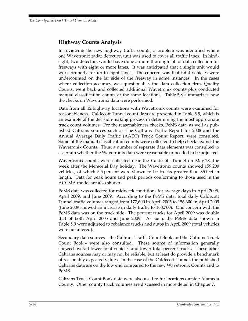
The Countywide Truck Travel Demand Model
5-14 Cambridge Systematics, Inc.
Highway Counts Analysis
In reviewing the new highway traffic counts, a problem was identified where one Wavetronix radar detection unit was used to cover all traffic lanes. In hind-sight, two detectors would have done a more thorough job of data collection for freeways with eight or more lanes. It was anticipated that a single unit would work properly for up to eight lanes. The concern was that total vehicles were undercounted on the far side of the freeway in some instances. In the cases where collection accuracy was questionable, the data collection firm, Quality Counts, went back and collected additional Wavetronix counts plus conducted manual classification counts at the same locations. Table 5.8 summarizes how the checks on Wavetronix data were performed.
Data from all 12 highway locations with Wavetronix counts were examined for reasonableness. Caldecott Tunnel count data are presented in Table 5.9, which is an example of the decision-making process in determining the most appropriate truck count volumes. For the reasonableness checks, PeMS data, as well as pub-lished Caltrans sources such as The Caltrans Traffic Report for 2008 and the Annual Average Daily Traffic (AADT) Truck Count Report, were consulted. Some of the manual classification counts were collected to help check against the Wavetronix Counts. Thus, a number of separate data elements was consulted to ascertain whether the Wavetronix data were reasonable or needed to be adjusted.
Wavertronix counts were collected near the Caldecott Tunnel on May 28, the week after the Memorial Day holiday. The Wavetronix counts showed 159,200 vehicles; of which 5.5 percent were shown to be trucks greater than 35 feet in length. Data for peak hours and peak periods conforming to those used in the ACCMA model are also shown.
PeMS data was collected for midweek conditions for average days in April 2005, April 2009, and June 2009. According to the PeMS data, total daily Caldecott Tunnel traffic volumes ranged from 177,600 in April 2005 to 156,300 in April 2009 (June 2009 showed an increase in daily traffic to 168,700). One concern with the PeMS data was on the truck side. The percent trucks for April 2009 was double that of both April 2005 and June 2009. As such, the PeMS data shown in Table 5.9 were adjusted to rebalance trucks and autos in April 2009 (total vehicles were not altered).
Secondary data sources – the Caltrans Traffic Count Book and the Caltrans Truck Count Book – were also consulted. These source of information generally showed overall lower total vehicles and lower total percent trucks. These other Caltrans sources may or may not be reliable, but at least do provide a benchmark of reasonably expected values. In the case of the Caldecott Tunnel, the published Caltrans data are on the low end compared to the new Wavetronix Counts and to PeMS.
Caltrans Truck Count Book data were also used to for locations outside Alameda County. Other county truck volumes are discussed in more detail in Chapter 7.

The
Cou
ntyw
ide
Tru
ck T
rave
l Dem
and
Mod
el
Cam
brid
ge S
yste
mat
ics,
Inc.
5-
15
Tabl
e 5.
8 A
sses
smen
t of H
ighw
ay T
ruck
Tra
ffic
Cou
nts
Loca
tion
Initi
al A
sses
smen
t of
New
Cou
nt Q
ualit
y M
anua
l Cla
ss C
ount
s C
olle
cted
? A
dditi
onal
Cou
nts
Col
lect
ed?
Follo
w-U
p A
sses
smen
t
SR 1
3 ne
ar I-
580
Goo
d
W
avet
roni
x da
ta a
ppea
rs re
ason
able
SR 2
4 at
Cal
deco
tt Tu
nnel
Ye
s W
avet
roni
x da
ta a
ppea
rs re
ason
able
I-80
at U
nive
rsity
Ave
Yes
Tr
uck
coun
t see
ms
high
; cou
ld b
e se
ason
al
I-680
Nea
r SR
262
Ye
s Ad
just
men
t of c
ount
dat
a w
as re
quire
d
I-680
At A
lcos
ta B
lvd
Yes
Adju
stm
ent o
f cou
nt d
ata
was
requ
ired
I-880
Sou
th o
f SR
262
G
ood
Wav
etro
nix
data
app
ears
reas
onab
le
I-880
at I
ndus
trial
Pkw
y
Ye
s W
avet
roni
x da
ta a
ppea
rs re
ason
able
I-880
at H
egen
berg
er R
oad
Ye
s
Wav
etro
nix
data
app
ears
reas
onab
le
I-880
bet
wee
n 5th
and
10th
Ave
Wav
etro
nix
data
app
ears
reas
onab
le
I-980
at 1
4th S
treet
Ye
s Tr
uck
coun
t may
be
high
; PeM
S no
t ava
ilabl
e
SR 2
38 b
et I-
880
& I-5
80
Goo
d
W
avet
roni
x da
ta a
ppea
rs re
ason
able
I-580
Eas
tern
Ala
Cou
nty
Ye
s
Adju
stm
ent o
f cou
nt d
ata
was
requ
ired
Not
es:
Initi
al a
sses
smen
t of n
ew c
ount
qua
lity
show
ed g
ood
coun
ts a
t thr
ee lo
catio
ns.
Man
ual t
ruck
cla
ssifi
catio
n co
unts
wer
e co
llect
ed a
t thr
ee o
ther
loca
tions
, and
wer
e in
clud
ed a
s pa
rt of
the
appr
oved
sco
pe o
f wor
k fo
r Qua
lity
Cou
nts.
The
man
ual c
lass
ifica
tion
coun
ts fo
r the
AM
and
PM
pea
k tw
o ho
urs
wer
e co
mpa
red
agai
nst t
he W
avet
roni
x co
unts
to h
elp
dete
rmin
e da
ta a
dequ
acy.
Afte
r con
side
ratio
n of
pot
entia
l pro
blem
s w
ith th
e W
avet
roni
x co
unts
, Qua
lity
Cou
nts
agre
ed to
con
duct
add
ition
al W
avet
roni
x C
ount
s, a
s w
ell a
s m
anua
l tru
ck c
lass
ifica
tions
co
unts
at t
hese
sam
e fiv
e lo
catio
ns.
(Not
e th
at a
ll m
anua
l cla
ssifi
catio
ns c
ount
s w
ere
colle
cted
at t
he s
ame
times
Wav
etro
nix
coun
ts w
ere
bein
g co
llect
ed).

The Countywide Truck Travel Demand Model
5-16 Cambridge Systematics, Inc.
Table 5.9 Traffic Count Data at SR 24 West Side of Caldecott Tunnel
Vehicle Length
0-35 Feet 35-61 Feet More Than 61 Feet Total Wavetronix Eastbound May 28, 2009 Daily 76,300 2,500 800 79,600 AM peak hour 3,400 200 0 3,600 PM peak hour 1 5,600 400 100 6,100 PM peak 2 hours 11,600 600 200 12,400 PM peak 4 hours 28,900 1,200 300 30,400 Wavetronix Westbound May 28, 2009 Daily 82,900 4,700 1,100 88,800 AM peak hour 5,400 600 100 6,200 PM peak hour 1 4,000 300 100 4,400 PM peak 2 hours 8,500 600 200 9,300 PM peak 4 hours 23,200 1,300 300 24,800 Wavetronix Both Directions May 28, 2009 Daily 159,200 7,300 1,900 168,400 AM peak hour 8,900 800 200 9,900 PM peak hour 1 9,600 700 200 10,500 PM peak 2 hours 20,100 1,200 300 21,600 PM peak 4 hours 52,100 2,500 600 55,200 PeMS
Total Auto Truck % Trucks Apr-2005 177,600 172,100 5,400 3.0% Apr-2009 156,300 147,100* 5,100* 3.3% Jun-2009 168,700 162,900 5,800 3.4% Caltrans Count Book AADT 2008 151,000 2006 150,000 Caltrans Truck Count Book % Truck 2007 2.2%
*April 2005 PeMS Auto and truck volumes adjusted to better match April 2005 and June 2009 records.
Overall, the Wavetronix counts fall comfortably within the total traffic counts obtained from PeMS. There is not a direct correspondence between the Wavetronix Counts and the PeMS counts, as the definitions for trucks are some-what different. However, this data review has allowed us to conclude the Wavetronix counts for the Caldecott Tunnel are indeed reasonable for use in the ACCMA truck model development efforts.

The Countywide Truck Travel Demand Model
Cambridge Systematics, Inc. 5-17
This station-by-station analysis revealed that seven of the highway count loca-tions appear reasonable, while the following five have some issues:
1. I-80/University Avenue. High Wavetronix truck counts.
2. I-880 between 5th and 10th Streets. High Wavetronix truck counts.
3. I-680/SR 262 (Mission Blvd). Low Wavetronix truck counts; an adjustment of the Wavetronix data was required.
4. I-680/Alcosta. Low Wavetronix truck counts; an adjustment of the Wavetronix data was required.
5. I-580/Flynn Road. Low Wavetronix truck counts; an adjustment of the Wavetronix data was required.
In these latter three instances, far side highway volumes were quite a bit lower than on the near side (where the Wavetronix unit was placed). In these instances, the adjustment was made on a daily basis to have far side volumes equal near side volumes (with the assumption that near side volumes are accurate).
Table 5.10 presents side-by-side comparisons of the new count stations with PeMS and the Caltrans sources. This includes some additional locations where new truck counts were not collected, but considered useful from a data analysis standpoint. These other locations include important truck routes in-between the new count locations.
Overall, the comparison of the Wavetronix data to other data sources was useful. There is a much greater sense the Wavetronix data are reasonable, given the direct comparisons to PeMS and to other Caltrans published values. In some cases, the PeMS data did not appear to be reasonable at some individual loca-tions – often with low volumes, or with auto/truck splits that were inconsistent with other data sources. In particular, it can be difficult to assess PeMS on a location-by-location basis. However, the exercise of comparing the various data sources provided the project team with good benchmarks for determining which data were most reasonable.
Arterial Counts Analysis
Arterial counts are summarized in Appendix A. Daily volumes range up to 64,000 total vehicles (at Mission Blvd between I-680 and I-880 in Fremont); and many locations have daily volumes in excess of 30,000 daily vehicles.
The arterials generally have less than 5 percent heavy trucks, except for the three locations near the Port of Oakland. At these locations, percent heavy trucks range from 20 to 40 percent. Total trucks generally range between 6 and 10 percent of total traffic. As noted earlier, it is not possible from these data to distinguish pickup trucks and vans (part of the autos category) as being for per-sonal use or commercial use.

The
Cou
ntyw
ide
Tru
ck T
rave
l Dem
and
Mod
el
5-18
C
ambr
idge
Sys
tem
atic
s, In
c.
Tabl
e 5.
10
Sum
mar
y of
Dai
ly F
reew
ay T
raffi
c an
d Tr
uck
Cou
nts
Loca
tion
Dai
ly W
avet
roni
x C
ount
s Pe
MS
Cal
tran
s R
esou
rces
Tota
l A
utos
Tr
ucks
%
Tru
cks
Tota
l A
uto
Truc
ks
% T
ruck
s 20
08
AA
DT
% T
ruck
D
eriv
ed
Truc
ks
AC
CM
A T
ruck
Mod
el C
ount
Sta
tions
SR
13
near
Jun
ctio
n 58
0
51,6
00
500
0.9%
–
– –
– 50
,000
1%
60
0 SR
24
at C
alde
cott
Tunn
el
168,
400
159,
200
9,20
0 5.
5%
156,
300
151,
200
5,10
0 3.
3%
160,
000
2%
3,80
0 I-8
0 at
Uni
vers
ity A
ve
261,
400
246,
700
14,6
00
5.6%
20
0,10
0 19
1,80
0 8,
200
4.1%
27
0,00
0 4%
10
,800
I-6
80 N
ear S
R 2
62
140,
000
132,
900
7,10
0 5.
1%
127,
600
121,
400
6,20
0 4.
9%
135,
000
7%
9,60
0 I-6
80 A
t Alc
osta
Blv
d 16
2,00
0 15
5,70
0 6,
300
3.9%
17
0,80
0 16
4,90
0 5,
900
3.5%
17
0,00
0 5%
9,
000
I-880
Sou
th o
f SR
262
20
6,80
0 19
8,90
0 7,
900
3.8%
–
– –
– 17
5,00
0 4%
7,
700
I-880
At I
ndus
trial
Pkw
y 21
2,40
0 20
0,60
0 11
,800
5.
6%
231,
000
213,
800
17,2
00
7.4%
20
0,00
0 6%
11
,800
I-8
80 A
t Heg
enbe
rger
Roa
d 21
0,40
0 19
3,80
0 16
,600
7.
9%
213,
900
198,
500
15,4
00
7.2%
20
0,00
0 8%
15
,200
I-8
80 b
et 5
th a
nd 1
0th A
venu
e 21
6,50
0 19
5,00
0 21
,500
9.
9%
– –
– –
225,
000
11%
24
,100
I-9
80 a
t 14th
Stre
et
79,2
00
77,9
00
1,20
0 1.
5%
– –
– –
75,0
00
7%
4,90
0 SR
238
bet
I-88
0 an
d I-5
80
141,
100
122,
100
19,0
00
13.5
%
– –
– 12
.5%
13
0,00
0 12
%
15,3
00
I-580
Eas
tern
Ala
med
a C
ount
y 14
3,60
0 12
5,60
0 18
,000
12
.5%
–
– –
13
8,00
0 13
%
17,3
00
Non
-Cou
nted
Loc
atio
ns o
f Int
eres
t I-8
80 n
ear W
est O
akla
nd B
ART
132,
000
128,
900
3,10
0 2.
3%
125,
000
–3
– I-5
80 n
ear D
ublin
/Ple
asan
ton
BAR
T 18
6,90
0 17
2,80
0 14
,200
7.
6%
193,
000
7%
13,1
00
I-580
Alb
any
near
I-80
95
,000
89
,100
5,
900
6.2%
85
,000
6%
5,
200
I-80
Bay
Brid
ge
243,
500
239,
100
4,40
0 1.
8%
255,
000
3%
7,10
0 SR
92
Dum
barto
n Br
idge
76
,200
66
,000
10
,300
13
.5%
62
,000
7%
4,
000
SR 8
4 Sa
n M
ateo
Brid
ge
102,
300
100,
300
2,00
0 2.
0%
93,0
00
6%
5,40
0
Not
es:
Dai
ly ra
dar d
etec
tor t
raffi
c co
unts
(usi
ng W
avet
roni
x un
its) w
ere
colle
cted
dire
ctly
for t
he A
CC
MA
truck
mod
el u
pdat
e. C
ount
s w
ere
colle
cted
at e
ach
loca
tion
by d
irect
ion
and
grou
ped
into
thre
e ve
hicl
e cl
assi
ficat
ion
bins
– u
nder
35
feet
(aut
os),
35 to
61
feet
, and
less
than
61
feet
(tru
cks)
. C
ount
s w
ere
colle
cted
ove
r 24
hour
s ov
er a
Tue
sday
, W
edne
sday
, or T
hurs
day.
Cou
nts
wer
e co
llect
ed in
May
and
Jun
e 20
10.
PeM
S da
ta a
re a
vera
ges
for J
une
2009
mid
-wee
k w
eekd
ays,
and
repr
esen
t dai
ly c
ondi
tions
.
Cal
trans
Res
ourc
es a
re 2
008
Cal
trans
Tra
ffic
Cou
nt B
ook
for 2
008,
and
Cal
trans
Ave
rage
Ann
ual D
aily
Tru
ck C
ount
boo
k.

The Countywide Truck Travel Demand Model
Cambridge Systematics, Inc. 6-1
6.0 Model Development and Validation In this chapter, new trip generation, distribution and assignment models are described. New truck traffic count data were very useful for overall model vali-dation. However, counts at selected locations do not provide the necessary data on total trips and travel patterns. Observed data needed to be augmented. For trip generation and distribution models, models were calibrated to synthesized ODME-derived observed trip ends and trip length frequency distributions. Model validation efforts for traffic assignment are also covered here.
For the purposes of delivering a new truck model system for ACCMA, observed data needed to be augmented. Although new traffic count data was boon for overall model validation, total trip and travel pattern data were nonexistent.
6.1 ODME-DERIVED TRIP TABLES ODME trip tables were developed with new traffic counts. The purpose of the ODME application was to create observed truck trip tables to evaluate model validation efforts. The ODME trip tables are not used as the model-developed trip tables.
Traffic counts at selected locations provide good information on the trucks crossing a specific point in the network. The specific traffic counts do not pro-vide an overall total of truck trips generated in Alameda County. The traffic counts also do not identify the origins and destinations or trip lengths for the truck trips, as a truck crossing a specific count location could be making a very long trip to Los Angeles or a short trip to the next city. In order to provide a modeling system, which can work for forecast scenarios, a set of equations need to be developed that estimate total truck trips and origins and destinations; and then this set of equations can be validated by comparing the model estimates to the actual traffic counts.
There were no additional survey data or other sources that could be used to create an observed set of total truck trip generation and origin-destination pat-terns. However, total trips and origin-destination patterns can be estimated using a mathematical process that fits an estimated starting trip matrix to the observed traffic counts. The ODME was selected to provide a target for cali-brating modeled trip ends (trip generation) and trip length frequency distribu-tions (trip distribution). This was seen as a cost-effective solution for development of observed data for which trip generation and distribution models could be developed.

The Countywide Truck Travel Demand Model
6-2 Cambridge Systematics, Inc.
The process starts with the existing model truck trip table as a “seed” (initial estimate) to ODME, and uses the observed truck counts as constraints. The ODME process adjusts the seed trip table until the assignment of that trip table most closely matches the counts. By comparing the results of the adjusted table to the estimate table from the prior iteration, we can see how and where to make adjustments. Two examples are given below for better understanding of the need for ODME and what it does here:
Example 1. Assume the numbers of trips in the new table (excluding intra-zonals, which are not assigned by the model and are not adjusted by ODME) are exactly twice that in the old table. Also, assume that the ratios comparing row and column sums between the new and old tables are all exactly twice the sums in the old table. The simple interpretation would be that the trip rates in the old model were all exactly 50 percent of what they should be to be validated against the counts. Double the trip rates and the new model that will be used in forecasting, when given base year employment data, will validate as closely as possible to counts, since that is what ODME does.
Example 2. Assume the observations are more complicated. The total truck trips ODME are twice the number of total truck trips in the old model, but the ratios of row and columns are not 2 to 1, and that is because some O-D pairs are not 2 to 1. For widely separated O-D pairs the ratio is 3, and for close in zones the ratios is 1. That is an indication that the friction factors are underestimating long-distance trips (it is one-third of what it should be), and are underestimating short-distance trips (the O-D pair ratio is only 1.0, while total trips have a ratio of 2.0). While the math is not as clean since the friction factors are an inverse exponential function, ODME adjusts the equations until the model closely matches the observed truck counts.
Varieties of different types of adjustments were made, but these examples are given to make the point of how the ODME trip tables will be used in the mod-eling. The idea is that ODME can show in what direction the truck model para-meters need to be adjusted. However, once those adjustments are made, there is never a need to use ODME again.
A number of ODME applications has been tested for this project. Evaluation of the different ODME applications is based on resultant traffic assignment valida-tion results against observed truck traffic counts. However, CS has found a method to create ODME-based trip tables for truck classes only. Previously, total vehicles were being subjected to ODME, and then truck trips (by class) were factored out.
Input Data
Truck counts collected within Alameda County were supplemented with other count data for other ACCMA model coverage areas outside Alameda County and used in the ODME procedure. The 2005 Caltrans Truck Count book was used to collect estimated total traffic and truck counts for a limited number of

The Countywide Truck Travel Demand Model
Cambridge Systematics, Inc. 6-3
locations in San Francisco, San Mateo, Santa Clara, Contra Costa, Solano, Napa, Sonoma, Marin, and San Joaquin Counties. Central locations were selected within each of these counties, as were external gateways (such as I-80 at the Solano/Napa county line and U.S. 101 at the Santa Clara/San Benito county line.
Figure 6.1 shows the geographic spread of the traffic and truck counts on free-ways, expressways, arterials, and collectors. The observed count database includes total daily traffic by vehicle class (automobile, small truck, medium truck, and combo truck). Table 6.1 shows the total number of count locations throughout the 10-county model coverage area and the number of new count locations within Alameda County. All of the compiled traffic and truck counts were used in the ODME procedure.
Methodology
The ODME procedure is an accepted practice that estimates trip tables based on traffic count data. Inputs include observed truck traffic counts on selected direc-tional links an initial estimate or “seed” matrix; in this case, the estimated truck O-D trip tables from the existing model. Using the seed matrix as a starting point and the observed volumes as control totals, the ODME process is executed within Cube Analyst to estimate O-D trip tables, which, when assigned to the network, produce link flows that optimally match the observed counts.
CS developed a process within Cube Analyst to preload auto trips into the traffic assignment, and therefore estimated only an ODME truck trip table. The assigned ODME-adjusted trips were being used as a validation check by com-paring summary statistics for each identified network link with observed counts, as well as by volume group and facility type. However, the existing truck trip tables estimated by the ODME process were not used as the final model result. Rather, they were used as a guide to calibrate the truck trip generation and dis-tribution models.
Traffic counts at selected locations provide good information on the trucks crossing a specific point in the network. The specific traffic counts do not pro-vide an overall total of truck trips generated in Alameda County. The traffic counts also do not identify the origins and destinations or trip lengths for the truck trips, as a truck crossing a specific count location could be making a very long trip to Los Angeles or a short trip to the next city. In order to provide a modeling system, which can work for forecast scenarios, a set of equations need to be developed that estimate total truck trips and origins and destinations, and then this set of equations can be validated by comparing the model estimates to the actual traffic counts.

The Countywide Truck Travel Demand Model
6-4 Cambridge Systematics, Inc.
Figure 6.1 Bay Areawide Count Locations used for ODME-based Trip Tables
Sources: New data collected for this study, and PeMS within Alameda County and Caltrans Truck Count
Book for locations outside Alameda County.
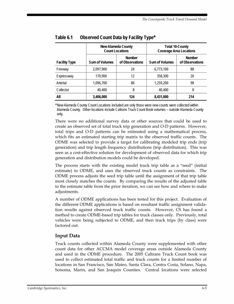
The Countywide Truck Travel Demand Model
Cambridge Systematics, Inc. 6-5
Table 6.1 Observed Count Data by Facility Type*
Facility Type
New Alameda County Count Locations
Total 10-County Coverage Area Locations
Sum of Volumes Number
of Observations Sum of Volumes Number
of Observations
Freeway 2,097,900 24 6,773,100 88
Expressway 170,900 12 358,300 20
Arterial 1,096,700 80 1,259,200 98
Collector 40,400 8 40,400 8
All 3,406,000 124 8,431,000 214
* New Alameda County Count Locations included are only those were new counts were collected within Alameda County. Other locations include Caltrans Truck Count Book volumes – outside Alameda County only.
There were no additional survey data or other sources that could be used to create an observed set of total truck trip generation and O-D patterns. However, total trips and O-D patterns can be estimated using a mathematical process, which fits an estimated starting trip matrix to the observed traffic counts. The ODME was selected to provide a target for calibrating modeled trip ends (trip generation) and trip length frequency distributions (trip distribution). This was seen as a cost-effective solution for development of observed data for which trip generation and distribution models could be developed.
The process starts with the existing model truck trip table as a “seed” (initial estimate) to ODME, and uses the observed truck counts as constraints. The ODME process adjusts the seed trip table until the assignment of that trip table most closely matches the counts. By comparing the results of the adjusted table to the estimate table from the prior iteration, we can see how and where to make adjustments.
A number of ODME applications has been tested for this project. Evaluation of the different ODME applications is based on resultant traffic assignment valida-tion results against observed truck traffic counts. However, CS has found a method to create ODME-based trip tables for truck classes only. Previously, total vehicles were being subjected to ODME, and then truck trips (by class) were factored out.
Input Data
Truck counts collected within Alameda County were supplemented with other count data for other ACCMA model coverage areas outside Alameda County and used in the ODME procedure. The 2005 Caltrans Truck Count book was used to collect estimated total traffic and truck counts for a limited number of locations in San Francisco, San Mateo, Santa Clara, Contra Costa, Solano, Napa, Sonoma, Marin, and San Joaquin Counties. Central locations were selected

The Countywide Truck Travel Demand Model
6-6 Cambridge Systematics, Inc.
within each of these counties, as were external gateways (such as I-80 at the Solano/Napa county line and U.S. 101 at the Santa Clara/San Benito county line.
Figure 6.1 shows the geographic spread of the traffic and truck counts on free-ways, expressways, arterials, and collectors. The observed count database includes total daily traffic by vehicle class (automobile, small truck, medium truck, and combo truck). Table 7.1 shows the total number of count locations throughout the 10-county model coverage area and the number of new count locations within Alameda County. All of the compiled traffic and truck counts were used in the ODME procedure.
Methodology
The ODME procedure is an accepted practice that estimates trip tables based on traffic count data. Inputs include observed truck traffic counts on selected direc-tional links and initial estimate or “seed” matrix; in this case, the estimated truck O-D trip tables from the existing model. Using the seed matrix as a starting point and the observed volumes as control totals, the ODME process is executed within Cube Analyst to estimate O-D trip tables, which, when assigned to the network, produce link flows that optimally match the observed counts.
CS developed a process within Cube Analyst to preload auto trips into the traffic assignment, and therefore estimated only an ODME truck trip table. The assigned ODME-adjusted trips were being used as a validation check by com-paring summary statistics for each identified network link with observed counts, as well as by volume group and facility type. However, the existing truck trip tables estimated by the ODME process were not used as the final model result. Rather, they were used as a guide to calibrate the truck trip generation and dis-tribution models.
Performance Measures
Model validation performance measures selected for this report were standard measures used for traffic assignment analysis. These measures included:
Simple difference between model volumes and observed counts.
Percent difference between model volumes and observed counts (or percent error).
Percent RMSE. This is an aggregate measure of all links; whereas, the differ-ence measures above are based on individual links.
For trip generation and distribution, aggregate measures were used to evaluate model validation. There was no real observed data to compared trip rates or trip length frequency distributions against; thus, ODME results were used to com-pare total truck trips by truck class.

The Countywide Truck Travel Demand Model
Cambridge Systematics, Inc. 6-7
For trip distribution, manual observations of the trip length frequency distribu-tions were used to for validation purposes. However, for both generation and distribution models, traffic assignment results were also evaluated.
Overall goodness of fit measure (R-squared) for the assigned total volumes. R-squared and RMSE values are based on standards developed from the FHWA Travel Model Validation and Reasonableness Checking Manual, and from the Travel Model Improvement Program White Paper on Model Validation24.
ACCMA Model Validation Results
The results of the 2005 Base Year ACCMA model’s daily assigned trips were compared to the observed counts. It should be noted that, while traffic counts inside and outside of Alameda County are used in the ODME process, the vali-dation statistics reported here are only for roadways in Alameda County. All presented results are given for total volumes. Daily volume aggregate perfor-mance of the current ACCMA model is summarized in a series in Tables 6.2 and 6.3.
Table 6.2 Existing Truck Model Validation Automobiles
Facility Type
Observed 2005 Base Year ACCMA Model –
Auto Volumes Target* % Error
Sum of Volumes
No. of Obs. Estimated
Percent RMSE
Percent Error Accept. Pref.
Freeway 1,866,100 24 1,745,900 18% -6% +/-7% +/-6%
Expressway 159,800 12 116,700 41% -27% +/-7% +/-6%
Arterial 1,029,900 80 1,190,400 62% 16% +/-15% +/-10%
Collector 28,400 8 15,900 97% -44% +/-25% +/-20%
All 3,084,200 124 3,068,800 36% 0% N/A N/A
24 National Cooperative Highway Research Program Report 255, Calibration and
Adjustment of System Planning Models, 1990; Travel Model Improvement Program, Federal Highway Administration, Model Validation and Reasonableness Checking Manual, 1997; and Travel Model Improvement Program, Federal Highway Administration, Travel Model Validation Practice Peer Exchange White Paper, December 3, 2008.

The Countywide Truck Travel Demand Model
6-8 Cambridge Systematics, Inc.
Table 6.3 Existing Truck Model Validation Trucks
Facility Type
Observed 2005 Base Year ACCMA Model –
Truck Volumes Target * % Error
Sum of Volumes
No. of Obs. Estimated
Percent RMSE
Percent Error Accept. Pref.
Freeway 231,900 24 240,436 55% 4% +/-7% +/-6%
Expressway 11,100 12 4,600 67% -59% +/-7% +/-6%
Arterial 66,800 80 59,600 99% -11% +/-15% +/-10%
Collector 12,100 8 5,800 69% -52% +/-25% +/-20%
All 321,800 124 310,400 93% -4% N/A N/A
Detailed, link-level model validation results for various time periods (AM one-hour, PM one-hour, PM two-hour, and PM four-hour) were also generated as part of this project. These tables are included in the report under Appendix B.
The percent error and percent RMSE values are higher than preferred for both automobiles and total trucks – with the exception of freeways. However, there are data issues that make producing significantly better results an extremely dif-ficult task. One issue is a standard one with any count program – there is signifi-cant daily variation in observed trucks or automobiles.
In addition, the 2009 counts were scaled back to 2005 conditions. Although there is a lot of supporting data for this conversion, undoubtedly errors were intro-duced as a result of this conversion. Finally, expressways and collectors represent very small sample sizes with correspondingly low volumes. These sample sizes are too small to produce reliable RMSEs.
As such, we believe these ODME values produce reasonable results; short of actually collecting new O-D data on truck travel patterns. However, the errors tend to be larger than were targeted.
6.2 TRIP GENERATION This section examines trip generation models that exist in the current ACCMA model, and new truck model options explored by the project team for the new truck model.

The Countywide Truck Travel Demand Model
Cambridge Systematics, Inc. 6-9
CS evaluated a number of new trip generation models for the ACCMA’s truck model project. These model types are described as follows:
Truck trip generation rates for internal25 trips only;
Use of PCEs are used in place of total (auto plus truck) volumes;
Port of Oakland considered a separate special generator; and
External truck trips modeled explicitly.
Various combinations of these factors were examined, and ultimately the final model included separate trip generation models for internal (i-i) trips apart from external trips (i-x, x-i, x-x). The Port of Oakland Seaport was treated as a special generator (with higher truck trip rates, and the use of PCEs rather than total vehicles). Table 6.4 summarizes the trip generation model coefficients.
Table 6.4 Truck Trip Generation Model Coefficients
LU/Sector
Production & Attraction Models
Small Medium Combo
Internal-Internal Trips
Manufacturing employment 0.0356 0.04459 0.02417
Retail employment 0.0387 0.03511 0.03736
Service employment 0.0351 0.06838 0.02239
Other employment 0.0719 0.06169 0.03021
Wholesale employment 0.0719 0.06169 0.03021
Agriculture employment 0.0719 0.06169 0.03021
Internal-External/External-Internal/External-External
Manufacturing employment 0.00610 0.01860
Retail employment
Service employment
Other employment 0.00130 0.00050 0.01180
Wholesale employment 0.00050 0.01260
Agriculture employment
The existing model was developed using separate trip generation rates for garage-based trucks versus nongaraged trucks. The new model does away with that distinction, as there is no new data on such distinctions.
25 Internal refers to travel solely within the 10-county model coverage area. External
refers to truck travel outside these 10 counties. External trips either stop within the model coverage area, or pass through the area.

The Countywide Truck Travel Demand Model
6-10 Cambridge Systematics, Inc.
Truck and total trip generation model validation results are summarized in Table 6.5. Total trucks are within two percent of the ODME-based truck trip ends, which are a substantial improvement over the existing model (see again Table 6.2).
Table 6.5 Trip Generation Model Validation Summary
Performance Measures ODME Final Trip Generation Rates
Total Volumes
Sum of Observed Volumes 3,406,000 3,406,000
Estimated Volumes 3,905,600 3,792,400
Percent Error 15% 11%
Percent Root-Mean-Square-Error 44% 39%
R-Squared .87 .90
Auto Volumes
Sum of Observed Volumes 3,084,200 3,084,200
Estimated Volumes 3,367,400 3,243,600
Percent Error 9% 5%
Percent Root-Mean-Square-Error 36% 37%
Truck Volumes
Sum of Observed Volumes 321,800 321,800
Estimated Volumes 400,200 327,300
Percent Error 24% 2%
Percent Root-Mean-Square-Error 103% 82%
Small Truck Volumes
Sum of Observed Volumes 69,594 69,594
Estimated Volumes 215,282 68,270
Percent Error 209% -2%
Percent Root-Mean-Square-Error 523% 127%
Medium Truck Volumes
Sum of Observed Volumes 76,500 76,525
Estimated Volumes 93,800 74,780
Percent Error 23% -2%
Percent Root-Mean-Square-Error 120% 112%
Combination Truck Volumes
Sum of Observed Volumes 175,700 175,700
Estimated Volumes 91,100 184,200
Percent Error -48% 5%
Percent Root-Mean-Square-Error 112% 93%
Although there are still some problems with the data (percent RMSE levels are higher than would be desired), the close matches of total trucks for each of the three vehicle classes do show a substantial improvement over the existing model.
The Countywide Truck Travel Demand Model
Cambridge Systematics, Inc. 6-11
Port of Oakland (Seaport) and Oakland Airport Special Generators
Special generators are usually added to travel demand models, where trip gener-ation rates applied to typical socioeconomic data, such as employment, will not produce reasonable trip productions and attractions for the nontypical location. For example, special generators for truck volumes are often used for seaports and airports. The major flows of goods are exchanged with no or very low man-ufacturing, industrial, and/or warehouse employment, which is typically the basis for estimating truck trip productions and attractions. Possible applications of special generators into the updated ACCMA truck model for the Oakland International Airport and the Port of Oakland were investigated
Port of Oakland
Table 6.6 and Figure 6.2 provide observed counts and estimated model volumes (without a special generator component) for locations at the Port of Oakland. The model, using only employment at the port zones to estimate truck produc-tions and attractions, significantly underestimates truck volumes at these loca-tions, estimating volumes of only approximately 10 percent of actual counts.
Since the model shows that employment is not a good indicator of truck flow, a special generator at this location was recommended to provide improvement to the model. The Port of Oakland special generator model created truck trip rates to match the base year count volumes at the three port gateways at Maritime Street, 7th Street, and Middle Harbor Way.
Table 6.7 and Figure 6.3 provide observed counts and estimated model volumes with a Port of Oakland special generator of 2,556 trucks produced and 2,556 trucks attracted. The addition of a special generator reduces error to -3% in the Port, a reduction of 87 percent of the error at the Port of Oakland Seaport without the added special generator truck trips.
Table 6.6 Port of Oakland Locations Count and Estimated Volumes Without 2005 Special Generator
Location Dir.
Total Truck Volumes
Count Estimated %Error
Maritime St south of Grand Ave SB 1,400 250 -82%
Maritime St south of Grand Ave NB 1,280 200 -82%
7th St west of I-880 WB 3,000 210 -93%
7th St west of I-880 EB 2,590 230 -91%
Middle Harbor Rd south of 3rd St SB 1,410 110 -92%
Middle Harbor Rd south of 3rd St NB 1,660 110 -94%
Total 11,340 1,130 -90%
Percent differences based on actual, not rounded, values.

The Countywide Truck Travel Demand Model
6-12 Cambridge Systematics, Inc.
Figure 6.2 Port of Oakland Locations Count and Estimated Volumes without 2005 Special Generator
Count Location XXXX Count Volume XXXX Estimated Volumes
Note: Percent differences based on actual, not rounded, values.
Maritime Street
7th Street
Middle Harbor Way

The Countywide Truck Travel Demand Model
Cambridge Systematics, Inc. 6-13
Table 6.7 Port of Oakland Locations Count and Estimated Assigned Volumes with 2005 Special Generator
Location Dir.
Total Truck Volumes
Count Estimated %Error
Maritime St south of Grand Ave SB 1,400 2,100 47%
Maritime St south of Grand Ave NB 1,300 2,200 75%
7th St west of I-880 WB 3,000 2,700 -10%
7th St west of I-880 EB 2,600 2,500 -2%
Middle Harbor Rd south of 3rd St SB 1,400 700 -48%
Middle Harbor Rd south of 3rd St NB 1,700 700 -57%
Total 11,300 11,000 -3%
Percent differences based on actual, not rounded, values.
Figure 6.3 Port of Oakland Locations Count and Estimated Assigned Volumes with 2005 Special Generator
Count Location XXXX Count Volume XXXX Estimated Volumes
7th Street
Middle Harbor Way
Maritime Street

The Countywide Truck Travel Demand Model
6-14 Cambridge Systematics, Inc.
Oakland Airport
While there are air cargo and distribution center facilities near airports, standard practice for the development of airport special generators limit the area to actual airport grounds within the gated areas of the airport, where there is otherwise no reason to produce and generate trucks based on employment. Nearby facilities related to the airport, such as air cargo and distribution centers, generally have employees for which their trips are more typically modeled in the traditional trip generation phase.
Table 6.8 and Figure 6.4 provide observed counts and estimated model volumes without an airport special generator. As shown in Figure 6.4, the model outputs show 0 (zero) truck volume on Airport Drive, south of Ron Cowan Parkway, but there are 1,450 model-estimated trucks just west of Airport Drive on a centroid connector where Air Cargo Way is actually located. The centroid that represents the Airport is simply placed further west, thus creating the shortest path when accessed via Ron Cowan Parkway and Air Cargo Way, and all trips (including auto trips) load onto that route. For the purposes of this analysis, those 1,450 model-estimated trucks can be compared to the 1,430 Airport Drive observed counts, as shown in Table 6.8.
Table 6.8 Oakland Airport Count and Estimated Assigned Volumes Without a Special Generator for Year 2005
Location Dir.
Total Truck Volumes
Count Estimated %Error
Hegenberger Rd btwn Edgewater Dr & I-880 SB On-Ramp SB 1,900 1,100 -41%
Hegenberger Rd btwn Edgewater Dr & I-880 SB On-Ramp NB 1,900 1,600 -13%
SR 61 (Doolittle Dr) between Swan Way & Langley St SB 400 200 -45%
SR 61 (Doolittle Dr) between Swan Way & Langley St NB 500 200 -54%
SR 61 (Doolittle Dr) between Davis St & Eden Rd SB 1,200 500 -55%
SR 61 (Doolittle Dr) between Davis St & Eden Rd NB 1,200 400 -69%
98th Ave between I-880 & Empire WB 1,900 1,700 -12%
98th Ave between I-880 & Empire EB 2,100 1,100 -50%
Doolittle Dr between Adams & Airport Dr SB 900 400 -52%
Doolittle Dr between Adams & Airport Dr NB 900 300 -67%
Airport drive south of Ron Cowan Parkway NB 1,400 1,500 2%
Airport drive south of Ron Cowan Parkway SB 1,400 1,500 2%
Total 15,767 10,491 -33%
Percent differences based on actual, not rounded, values.

The Countywide Truck Travel Demand Model
Cambridge Systematics, Inc. 6-15
Figure 6.4 Oakland Airport Count and Estimated Assigned Volumes Without a Special Generator
Count LocationXXXX Count VolumeXXXX Estimated Volumes
Oakland Airport
Overall, the percent errors may seem high for locations near the Airport, but it is important to note the low volumes of these facilities. Regional models generally do not perform well in small areas with large zones, and are not developed with the intention to accurately forecast low-volume facilities. For facilities with less than 10,000 average daily traffic, industry standards mark the acceptable percent error to be ±50 percent, and the preferable percent error to be ±25 percent.26 Here, all count locations have daily volumes much less than 10,000 vehicles. It should also be noted that model volumes at the actual airport access road are estimated at a 2-percent difference from the observed counts, indicating well-modeled volumes to and from the airport.
Truck modeling sometimes utilizes special generators for facilities that with little or no socioeconomic data for which to project trip productions and attractions. For the updated ACCMA truck model, it was determined that Port of Oakland locations were not being modeled sufficiently; and a special generator was developed and implemented to produce more accurate results.
Without an airport special generator, the model performed well for truck trips directly in and out of the Airport. Some nearby locations, however, produced less than preferable estimated volumes, but are still within acceptable ranges. Regional models are not intended to produce highly accurate volumes within small areas and on low-volumes roads.
26 Florida DOT Model Calibration and Validation Standards Final Report 2008.

The Countywide Truck Travel Demand Model
6-16 Cambridge Systematics, Inc.
The recommended course of action is to compare the model’s network and traffic analysis zones with actual conditions and possibly move centroid connectors, which is often a source of error in small areas with large zones. A review of the socioeconomic data in the area may also be warranted. An airport special gene-rator, however, is not recommended because the employment-based truck trip ends appear to reasonably match the observed counts to and from the airport cargo gate (refer back to Table 6.8 and Figure 6.4).
6.3 TRIP DISTRIBUTION Trip Length Frequency Distributions (TLFD) were prepared and examined for the original and the ODME tables. A comparison of these distributions guided not only changes to the friction factors, but also changes to the use of impedance variables. Changes to the TLFD for IE/EI and I-I truck trips can be seen in Figures 6.5 through 6.10. The existing model TLFD using the AM skim times, which were the impedances used in the auto distribution, differed considerably from the distribution of the ODME-adjusted table for IE/EI trips. When the off peak skims were used as the impedance variable, as well as minor changes to the friction factors, the TLFD more closely matched that of the ODME table. While the adjustment was not as dramatic for other trips types, the ODME table was used to determine what changes should be made to the trip distribution process.
6.4 TRAFFIC ASSIGNMENT While not actually an adjustment which was guided by the ODME, the original model’s assignment was of vehicles and the link capacities were expressed in terms of vehicles per hour, with a truck being one vehicle. An improvement was made by applying a PCE, factors of 1.5 for medium trucks and 2.0 for combo trucks, to the truck tables and expressing the link capacities in terms of passenger cars per hour. This was done in a multiclass assignment with autos, which changed the assignment of all vehicles.
The rationale for this change is that since trucks are longer than average automo-biles, they use more roadway, and thus take up more available capacity. For this reason, PCE factors have been used during the assignment step of the ACCMA travel demand model.
The final selected PCEs convert to the exact same roadway volumes. However, the PCEs provide a better way to account for the differential capacities between trucks and automobiles. In particular, the use of PCEs recognizes the impacts of trucks on high-truck volume facilities from low-truck volume facilities. Put another way, Consider two freeways with equal traffic volumes per lane per hour. A freeway with a high number of trucks (example, I-880 in Oakland) will show a worse level of service than a facility with low-truck volumes (for exam-ple, SR 31 in Oakland). This differentiation can only be observed through a PCE analysis.

The
Cou
ntyw
ide
Tru
ck T
rave
l Dem
and
Mod
el
Cam
brid
ge S
yste
mat
ics,
Inc.
6-
17
Figu
re 6
.5
Trip
Len
gth
Freq
uenc
y D
istr
ibut
ion
for I
E/EI
Sm
all T
ruck
Trip
s
0%5%10%
15%
20%
050
100
150
200
250
300
Tra
vel
Tim
e (
min
)
Percent of IEEI Small Truck Trips
OD
ME
Ori
gin
al T
ruck
Fri
ctio
n F
act
ors
and
AM
Pe
ak
Hw
y S
kim
s
Fin
al -
Mo
difi
ed
Tru
ck F
rict
ion
Fa
cto
rs, O
ff P
ea
k H
wy
Ski
ms,
Re
vise
d P
CE
Ca
pa
citie
s
N
ote:
Ex
tern
al tr
ips
can
have
one
leg
(orig
in o
r des
tinat
ion)
with
in m
odel
cov
erag
e ar
ea o
r can
be
thro
ugh
trips
.

The
Cou
ntyw
ide
Tru
ck T
rave
l Dem
and
Mod
el
6-18
C
ambr
idge
Sys
tem
atic
s, In
c.
Figu
re 6
.6
Trip
Len
gth
Freq
uenc
y D
istr
ibut
ion
for I
E/EI
Med
ium
Tru
ck T
rips
0%
5%
10
%
15
%
20
%
05
010
01
50
200
25
03
00
Tra
vel
Tim
e (
min
)
Percent of IEEI Medium Truck Trips
OD
ME
Ori
gina
l Tru
ck F
rict
ion
Fa
cto
rs a
nd A
M P
eak
Hw
y S
kim
s
Fin
al -
Mod
ified
Tru
ck F
rictio
n F
act
ors
, Off
Pe
ak
Hw
yS
kim
s, R
evi
sed
PC
E C
ap
aciti
es
N
ote:
Ex
tern
al tr
ips
can
have
one
leg
(orig
in o
r des
tinat
ion)
with
in m
odel
cov
erag
e ar
ea o
r can
be
thro
ugh
trips
.

The
Cou
ntyw
ide
Tru
ck T
rave
l Dem
and
Mod
el
Cam
brid
ge S
yste
mat
ics,
Inc.
6-
19
Figu
re 6
.7
Trip
Len
gth
Freq
uenc
y D
istr
ibut
ion
for E
xter
nal C
ombi
natio
n Tr
uck
Trip
s
0%2%4%6%8%10%
050
100
150
200
250
300
Tra
ve
l Tim
e (
min
)
Percent of IEEI Combo Truck Trips
OD
ME
Ori
gina
l Tru
ck F
rict
ion
Fa
cto
rs a
nd A
M P
ea
k H
wy
Ski
ms
Fin
al -
Mo
difi
ed
Tru
ck F
rict
ion
Fa
cto
rs, O
ff P
ea
k H
wy
Ski
ms,
Re
vise
d P
CE
Ca
pa
citie
s
N
ote:
Ex
tern
al tr
ips
can
have
one
leg
(orig
in o
r des
tinat
ion)
with
in m
odel
cov
erag
e ar
ea o
r can
be
thro
ugh
trips
.
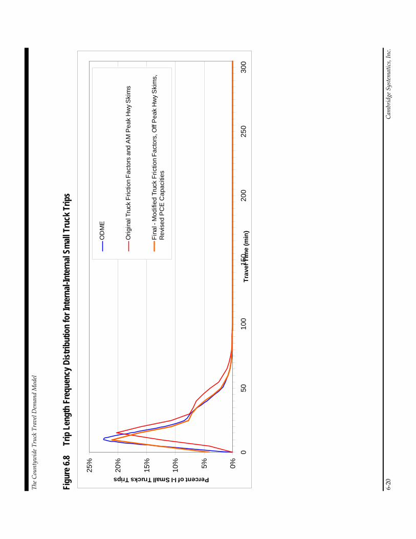
The
Cou
ntyw
ide
Tru
ck T
rave
l Dem
and
Mod
el
6-20
C
ambr
idge
Sys
tem
atic
s, In
c.
Figu
re 6
.8
Trip
Len
gth
Freq
uenc
y D
istr
ibut
ion
for I
nter
nal-I
nter
nal S
mal
l Tru
ck T
rips
0%5%10%
15%
20%
25%
050
100
150
200
250
300
Tra
ve
l Tim
e (
min
)
Percent of I-I Small Trucks Trips
OD
ME
Ori
gin
al T
ruck
Fri
ctio
n F
act
ors
and
AM
Pe
ak
Hw
y S
kim
s
Fin
al -
Mo
difi
ed
Tru
ck F
rict
ion
Fa
cto
rs, O
ff P
ea
k H
wy
Ski
ms,
Re
vise
d P
CE
Ca
pa
citie
s

The
Cou
ntyw
ide
Tru
ck T
rave
l Dem
and
Mod
el
Cam
brid
ge S
yste
mat
ics,
Inc.
6-
21
Figu
re 6
.9
Trip
Len
gth
Freq
uenc
y D
istr
ibut
ion
for I
nter
nal-I
nter
nal M
ediu
m T
ruck
Trip
s
0%
5%
10
%
15
%
20
%
25
%
30
%
05
01
00
15
02
00
25
03
00
Tra
ve
l Tim
e (
min
)
Percent of I-I Medium Truck Trips)
OD
ME
Orig
inal
Tru
ck F
rictio
n F
acto
rs a
nd A
M P
eak
Hw
y S
kim
s
Fin
al -
Mod
ified
Tru
ck F
rictio
n F
acto
rs, O
ff P
eak
Hw
y S
kim
s,R
evis
ed P
CE
Cap
aciti
es

The
Cou
ntyw
ide
Tru
ck T
rave
l Dem
and
Mod
el
6-22
C
ambr
idge
Sys
tem
atic
s, In
c.
Figu
re 6
.10
Trip
Len
gth
Freq
uenc
y D
istr
ibut
ion
for I
nter
nal-I
nter
nal C
ombi
natio
n Tr
uck
Trip
s
0%3%6%9%12%
15%
050
100
150
200
250
300
Tra
ve
l Tim
e (
min
)
Percent of I-I Combo Truck Trips)
OD
ME
Ori
gin
al T
ruck
Fri
ctio
n F
act
ors
and
AM
Pe
ak
Hw
y S
kim
s
Fin
al -
Mo
difi
ed
Tru
ck F
rict
ion
Fa
cto
rs, O
ff P
ea
k H
wy
Ski
ms,
Re
vise
d P
CE
Ca
pa
citie
s
The Countywide Truck Travel Demand Model
Cambridge Systematics, Inc. 6-23
Tables 6.9 through 6.13 present the final year 2005 traffic assignment validation results. Each table shows one of the five ACCMA model time periods – Daily, AM peak hour, PM peak hour, PM peak two hours, and PM peak four hours. Each of the tables presents the three truck classes, as well as total vehicles (including all trucks and autos).
Truck Prohibitions
Jurisdictions have imposed truck prohibitions on a number of area roadways, notably I-580 through Oakland. These bans also apply to a number of local roads. A review of truck bans was summarized during this study, and is included in roadway maps that include trucking designations along with other data (such as count station locations relevant for this study). Please see Appendix B for these maps.
The project team considered adding the truck prohibitions to the model system, but with the exception of I-580 they were not included. There were a number of reasons for not including the truck prohibitions. First, there are various defini-tions of truck prohibitions across different jurisdictions. In addition, the truck bans tend to be applied to roadways that would not generally have much, if any, heavy truck traffic (the bans tend to be applied in residential locations). In one case – the Caldecott Tunnel – the prohibition is a time period restriction to a class of trucks not distinguished in the ACCMA truck model. Finally, and of greatest concern was applying the prohibitions could result in trucks not being able to get on or off the network, depending on how travel analysis zone centroids were coded.

The
Cou
ntyw
ide
Tru
ck T
rave
l Dem
and
Mod
el
6-24
C
ambr
idge
Sys
tem
atic
s, In
c.
Tabl
e 6.
9 Ye
ar 2
005
Dai
ly T
raffi
c A
ssig
nmen
t Val
idat
ion
by V
ehic
le C
lass
and
Fac
ility
Typ
e
Faci
lity
Type
No.
of
O
bs.
Smal
l Tru
cks
Med
ium
Tru
cks
Com
bo T
ruck
s
Obs
erve
d Vo
lum
e Es
timat
ed
Volu
me
Perc
ent
RM
SE
Perc
ent
Erro
r O
bser
ved
Volu
me
Estim
ated
Vo
lum
e Pe
rcen
t R
MSE
Pe
rcen
t Er
ror
Obs
erve
d Vo
lum
e Es
timat
ed
Volu
me
Perc
ent
RM
SE
Perc
ent
Erro
r
Free
way
24
31
,900
48
,400
12
4%
52%
60
,700
49
,700
66
%
-18%
13
9,30
0 14
2,40
0 56
%
2%
Expr
essw
ay
12
4,90
0 1,
600
76%
-6
8%
2,20
0 1,
900
77%
-1
4%
4,10
0 1,
200
84%
-7
1%
Arte
rial
80
31,4
00
17,3
00
91%
-4
5%
11,2
00
18,5
00
175%
65
%
24,1
00
23,7
00
159%
-2
%
Col
lect
or
8 1,
400
500
82%
-6
5%
2,40
0 1,
200
79%
-5
0%
8,20
0 4,
000
73%
-5
1%
All
124
69,6
00
67,8
00
138%
-3
%
76,5
00
71,3
00
122%
-7
%
175,
700
171,
300
103%
-2
%
Faci
lity
Type
No.
of
O
bs.
Tota
l Aut
os a
nd T
ruck
s Ta
rget
% E
rror
Obs
erve
d Vo
lum
e Es
timat
ed
Volu
me
Perc
ent
RM
SE
Perc
ent
Erro
r A
ccep
t. Pr
ef.
Free
way
24
2,
097,
900
1,98
6,40
0 17
%
-5%
+/
-7%
+/
-6%
Expr
essw
ay
12
170,
900
121,
300
42%
-2
9%
+/-1
0%
+/-7
%
Arte
rial
80
1,09
6,70
0 1,
250,
000
60%
14
%
+/-1
5%
+/-1
0%
Col
lect
or
8 40
,400
21
,600
76
%
-46%
+/
-25%
+/
-20%
All
124
3,40
5,90
0 3,
379,
300
34%
-1
%
N/A
N
/A

The
Cou
ntyw
ide
Tru
ck T
rave
l Dem
and
Mod
el
Cam
brid
ge S
yste
mat
ics,
Inc.
6-
25
Tabl
e 6.
10
Year
200
5 A
M P
eak-
Hou
r Tra
ffic
Ass
ignm
ent V
alid
atio
n by
Veh
icle
Cla
ss a
nd F
acili
ty T
ype
Faci
lity
Type
N
o. o
f O
bs.
Smal
l Tru
cks
Med
ium
Tru
cks
Com
bo T
ruck
s
Obs
erve
d Vo
lum
e Es
timat
ed
Volu
me
Perc
ent
RM
SE
Perc
ent
Erro
r O
bser
ved
Volu
me
Estim
ated
Vo
lum
e Pe
rcen
t R
MSE
Pe
rcen
t Er
ror
Obs
erve
d Vo
lum
e Es
timat
ed
Volu
me
Perc
ent
RM
SE
Perc
ent
Erro
r
Free
way
24
1
,900
2
,900
17
6%
51%
3
,600
3
,000
79
%
-17%
8
,100
8
,100
63
%
2%
Expr
essw
ay
12
300
2
00
57%
-3
1%
100
2
00
108%
56
%
300
2
00
105%
-7
1%
Arte
rial
80
2,0
00
1,4
00
119%
-2
9%
700
1
,500
30
1%
106%
1
,600
1
,800
27
6%
-2%
Col
lect
or
8
100
–
77
%
-63%
2
00
100
10
2%
-51%
6
00
300
82
%
-51%
All
124
4
,300
4
,500
19
0%
6%
4,6
00
4,8
00
149%
3%
1
0,60
0
10,
400
12
1%
-2%
Faci
lity
Type
N
o. o
f O
bs.
Tota
l Aut
os a
nd T
ruck
s Ta
rget
% E
rror
Obs
erve
d Vo
lum
e Es
timat
ed
Volu
me
Perc
ent
RM
SE
Perc
ent
Erro
r A
ccep
t. Pr
ef.
Free
way
24
1
31,4
00
123
,600
27
%
-6%
+/
-7%
+/
-6%
Expr
essw
ay
12
10,
700
1
4,10
0
59%
32
%
+/-1
0%
+/-7
%
Arte
rial
80
66,
100
8
6,40
0
80%
31
%
+/-1
5%
+/-1
0%
Col
lect
or
8
2,8
00
2,1
00
35%
-2
6%
+/-2
5%
+/-2
0%
All
124
2
11,0
00
226
,200
49
%
7%
N/A
N
/A

The
Cou
ntyw
ide
Tru
ck T
rave
l Dem
and
Mod
el
6-26
C
ambr
idge
Sys
tem
atic
s, In
c.
Tabl
e 6.
11
Year
200
5 PM
Pea
k-H
our T
raffi
c A
ssig
nmen
t Val
idat
ion
by V
ehic
le C
lass
and
Fac
ility
Typ
e
Faci
lity
Type
No.
of
O
bs.
Smal
l Tru
cks
Med
ium
Tru
cks
Com
bo T
ruck
s
Obs
erve
d Vo
lum
e Es
timat
ed
Volu
me
Perc
ent
RM
SE
Perc
ent
Erro
r O
bser
ved
Volu
me
Estim
ated
Vo
lum
e Pe
rcen
t R
MSE
Pe
rcen
t Er
ror
Obs
erve
d Vo
lum
e Es
timat
ed
Volu
me
Perc
ent
RM
SE
Perc
ent
Erro
r
Free
way
24
1,
900
2,40
0 13
3%
26%
3,
700
2,70
0 79
%
-27%
8,
300
7,80
0 68
%
-6%
Expr
essw
ay
12
300
300
52%
-9
%
200
300
115%
82
%
300
300
94%
-2
1%
Arte
rial
80
1,80
0 1,
200
139%
-3
4%
800
1,40
0 20
1%
71%
1,
600
1,90
0 28
3%
23%
Col
lect
or
8
100
– 87
%
-56%
20
0 10
0 99
%
-37%
40
0 30
0 84
%
-17%
All
124
4,
100
3,90
0 16
1%
-4%
4,
900
4,50
0 14
3%
-7%
10
,600
10
,300
13
1%
-2%
Faci
lity
Type
No.
of
O
bs.
Tota
l Aut
os a
nd T
ruck
s Ta
rget
% E
rror
Obs
erve
d Vo
lum
e Es
timat
ed
Volu
me
Perc
ent
RM
SE
Perc
ent
Erro
r A
ccep
t. Pr
ef.
Free
way
24
12
8,50
0 12
8,00
0 25
%
0%
+/-7
%
+/-6
%
Expr
essw
ay
12
13,5
00
18,7
00
55%
39
%
+/-1
0%
+/-7
%
Arte
rial
80
77,2
00
96,1
00
72%
24
%
+/-1
5%
+/-1
0%
Col
lect
or
8
2,80
0 1,
800
56%
-3
7%
+/-2
5%
+/-2
0%
All
124
22
2,00
0 24
4,60
0 46
%
10%
N
/A
N/A

The
Cou
ntyw
ide
Tru
ck T
rave
l Dem
and
Mod
el
Cam
brid
ge S
yste
mat
ics,
Inc.
6-
27
Tabl
e 6.
12
Year
200
5 PM
Pea
k Tw
o H
ours
Tra
ffic
Ass
ignm
ent V
alid
atio
n by
Veh
icle
Cla
ss a
nd F
acili
ty T
ype
Faci
lity
Type
No.
of
O
bs.
Smal
l Tru
cks
Med
ium
Tru
cks
Com
bo T
ruck
s
Obs
erve
d Vo
lum
e Es
timat
ed
Volu
me
Perc
ent
RM
SE
Perc
ent
Erro
r O
bser
ved
Volu
me
Estim
ated
Vo
lum
e Pe
rcen
t R
MSE
Pe
rcen
t Er
ror
Obs
erve
d Vo
lum
e Es
timat
ed
Volu
me
Perc
ent
RM
SE
Perc
ent
Erro
r
Free
way
24
3,
800
5,20
0 13
9%
36%
7,
300
5,80
0 82
%
-21%
16
,400
15
,000
69
%
-8%
Expr
essw
ay
12
600
500
56%
-1
2%
300
600
115%
84
%
600
500
87%
-2
2%
Arte
rial
80
3,60
0 2,
400
136%
-3
3%
1,60
0 2,
800
199%
75
%
3,00
0 3,
700
264%
21
%
Col
lect
or
8
200
100
86%
-5
7%
300
200
102%
-4
2%
800
600
85%
-2
6%
All
124
8,
200
8,20
0 16
5%
0%
9,50
0 9,
400
146%
-2
%
20,8
00
19,8
00
131%
-5
%
Faci
lity
Type
No.
of
O
bs.
Tota
l Aut
os a
nd T
ruck
s Ta
rget
% E
rror
Obs
erve
d Vo
lum
e Es
timat
ed
Volu
me
Perc
ent
RM
SE
Perc
ent
Erro
r A
ccep
t. Pr
ef.
Free
way
24
25
2,40
0 25
0,00
0 23
%
-1%
+/
-7%
+/
-6%
Expr
essw
ay
12
28,5
00
38,2
00
48%
34
%
+/-1
0%
+/-7
%
Arte
rial
80
162,
600
196,
500
67%
21
%
+/-1
5%
+/-1
0%
Col
lect
or
8
7,00
0 3,
900
59%
-4
4%
+/-2
5%
+/-2
0%
All
124
45
0,50
0 48
8,60
0 43
%
8%
N/A
N
/A

The
Cou
ntyw
ide
Tru
ck T
rave
l Dem
and
Mod
el
6-28
C
ambr
idge
Sys
tem
atic
s, In
c.
Tabl
e 6.
13
Year
200
5 PM
Pea
k Fo
ur H
ours
Tra
ffic
Ass
ignm
ent V
alid
atio
n by
Veh
icle
Cla
ss a
nd F
acili
ty T
ype
Faci
lity
Type
No.
of
O
bs.
Smal
l Tru
cks
Med
ium
Tru
cks
Com
bo T
ruck
s
Obs
erve
d Vo
lum
e Es
timat
ed
Volu
me
Perc
ent
RM
SE
Perc
ent
Erro
r O
bser
ved
Volu
me
Estim
ated
Vo
lum
e Pe
rcen
t R
MSE
Pe
rcen
t Er
ror
Obs
erve
d Vo
lum
e Es
timat
ed
Volu
me
Perc
ent
RM
SE
Perc
ent
Erro
r
Free
way
24
7,
700
10,9
00
132%
41
%
14,7
00
11,7
00
77%
-2
1%
33,7
00
30,4
00
65%
-1
0%
Expr
essw
ay
12
1,10
0 1,
100
36%
-3
%
600
1,30
0 14
8%
112%
1,
200
1,30
0 10
7%
5%
Arte
rial
80
7,10
0 5,
000
132%
-3
0%
3,10
0 5,
700
194%
81
%
5,90
0 7,
900
242%
33
%
Col
lect
or
8
300
100
82%
-5
0%
600
400
90%
-3
5%
1,50
0 1,
100
67%
-2
4%
All
124
16
,200
17
,100
15
7%
5%
19,0
00
19,1
00
139%
0%
42
,300
40
,700
12
4%
-4%
Faci
lity
Type
No.
of
O
bs.
Tota
l Aut
os a
nd T
ruck
s Ta
rget
% E
rror
Obs
erve
d Vo
lum
e Es
timat
ed
Volu
me
Perc
ent
RM
SE
Perc
ent
Erro
r A
ccep
t. Pr
ef.
Free
way
24
52
0,50
0 47
6,80
0 22
%
-8%
+/
-7%
+/
-6%
Expr
essw
ay
12
53,6
00
71,3
00
48%
33
%
+/-1
0%
+/-7
%
Arte
rial
80
313,
300
379,
300
63%
21
%
+/-1
5%
+/-1
0%
Col
lect
or
8
12,9
00
6,50
0 65
%
-49%
+/
-25%
+/
-20%
All
124
90
0,30
0 93
3,90
0 41
%
4%
N/A
N
/A

The Countywide Truck Travel Demand Model
Cambridge Systematics, Inc. 7-1
7.0 2015 and 2035 Forecasts This section examines forecasts of truck volumes by class of truck and time period for the years 2015 and 2035. Also shown are forecasts of Port of Oakland Seaport growth assumptions, as used for the special generator model.
7.1 TRUCK FORECASTS ACCMA truck forecasts were created for years 2015 and 2035. As with the year 2005 base year, forecasts were prepared for five time periods: Daily, AM peak hour, PM peak hour, PM peak two hours, and PM peak four hours.
Overall traffic is projected to increase between 10 and 17 percent over the 10-year period between 2005 and 2015. Truck traffic, in aggregate, is projected to grow at roughly the same rate as total traffic, including autos. Growth in combo trucks is projected to rise somewhat faster than for small and medium trucks, and for autos, as shown in Table 7.1.
For 2035, growth rates range roughly between 40 and 60 percent – depending on time of day. Overall, the rate of growth to 2035 is projected to be faster beyond 2015 than between 2005 and 2015. There is little difference in growth between peak periods and daily conditions, as shown in Table 7.2.
Figures 7.1 through 7.4 display validation and forecast results for the a.m. peak hour at four specific areas in Alameda County. Locations selected include I-80 in Berkeley near University Avenue, I-880 in Oakland near Oakland Airport, I-880 in Hayward and Union City near Industrial Boulevard, and I-580 in eastern Alameda County.
Table 7.3 examines annualized rates of growth for each vehicle class. As noted above, growth rates are somewhat higher after 2015 than between 2015 and 2035. This is true for small and medium trucks, and for autos. Combo trucks have consistent rates of growth. Overall growth rates range from 1.0 percent to 1.6 percent per year, depending on time period and vehicle type.

The
Cou
ntyw
ide
Tru
ck T
rave
l Dem
and
Mod
el
7-2
C
ambr
idge
Sys
tem
atic
s, In
c.
Tabl
e 7.
1 Ye
ar 2
015
Traf
fic A
ssig
nmen
t Val
idat
ion
by V
ehic
le C
lass
and
Fac
ility
Typ
e
Dai
ly
Yea
r 20
05
Vol
um
e
Yea
r 20
15
Vol
um
e C
ha
% C
ha
Yea
r 20
05
Vol
um
e
Yea
r 20
15
Vol
um
e C
ha
% C
ha
Yea
r
2005
Vol
um
e
Yea
r
2015
Vol
um
e C
ha
% C
ha
Yea
r 20
05
Vol
um
e
Yea
r 20
15
Vol
um
e C
ha
% C
ha
Free
way
24
48,6
00
53,0
00
4,40
0
9%
50,2
00
56,0
00
5,80
0
12
%24
14
6,90
0
169,
200
22
,300
15%
1,98
5,10
0
2,15
0,40
0
165,
300
8%
Exp
ress
way
12
1,50
0
2,
600
1,
100
73%
1,90
0
3,
000
1,
100
58%
12
1,20
0
3,
200
2,00
0
16
7%12
1,10
0
17
8,00
0
56
,900
47%
Art
eria
l 80
17
,300
19
,600
2,
300
13%
18,5
00
21,1
00
2,60
0
14
%80
22
,900
26,7
00
3,
800
17%
1,24
6,20
0
1,37
2,90
0
126,
700
10
%
Col
lect
or8
1,
000
1,20
0
200
20%
2,30
0
2,
800
50
0
22
%8
7,70
0
9,
800
2,10
0
27
%27
,000
42
,900
15
,900
59%
All
124
68,3
00
76,4
00
8,10
0
12
%72
,800
82
,900
10
,100
14%
124
178,
500
20
8,90
0
30,4
00
17
%3,
379,
500
3,
744,
200
36
4,70
0
11%
AM
Pea
k 1
Hou
r
Free
way
24
2,90
0
3,
100
20
0
7%
3,10
0
3,
400
30
0
10
%24
8,
400
9,40
0
1,
000
12%
123,
500
137,
400
13,9
00
11
%
Exp
ress
way
12
200
30
0
10
0
50
%20
0
300
100
50%
12
200
400
200
100%
14,2
00
19,9
00
5,70
0
40%
Art
eria
l 80
1,
400
1,60
0
200
14%
1,60
0
1,
800
20
0
13
%80
1,
900
2,10
0
20
0
11
%86
,700
97
,800
11
,100
13%
Col
lect
or8
10
0
100
-
0%
200
30
0
10
0
50
%8
600
800
200
33%
2,60
0
3,40
0
80
0
31
%A
ll12
4
4,
600
5,20
0
600
13%
5,10
0
5,
800
70
0
14
%12
4
11
,100
12,7
00
1,
600
14%
227,
000
258,
500
31,5
00
14
%
PM
Pea
k 1
Hou
r
Free
way
24
2,40
0
2,
700
30
0
13
%2,
700
3,10
0
400
15%
24
8,10
0
9,
700
1,60
0
20
%12
7,90
0
13
8,60
0
10
,700
8%
Exp
ress
way
12
300
30
0
-
0%
300
40
0
10
0
33
%12
30
0
40
0
10
0
33
%18
,600
23
,400
4,
800
26
%
Art
eria
l 80
1,
200
1,30
0
100
8%1,
400
1,60
0
200
14%
80
2,00
0
2,
000
-
0%97
,700
10
6,40
0
8,
700
9%
Col
lect
or8
10
0
100
-
0%20
0
300
100
50%
8
60
0
80
0
20
0
33
%2,
200
3,
200
1,00
0
45%
All
124
4,00
0
4,
500
50
0
13
%4,
700
5,30
0
600
13%
124
11,0
00
12
,900
1,90
0
17
%24
6,40
0
27
1,60
0
25
,200
10%
PM
Pea
k 2
Hou
r
Free
way
24
5,20
0
5,
700
50
0
10
%5,
800
6,60
0
800
14%
24
15,6
00
18
,500
2,90
0
19
%25
0,10
0
27
0,90
0
20
,800
8%
Exp
ress
way
12
500
60
0
10
0
20
%60
0
700
100
17%
12
500
800
300
60%
38,4
00
47,1
00
8,70
0
23%
Art
eria
l 80
2,
400
2,70
0
300
13%
2,90
0
3,
200
30
0
10
%80
3,
700
3,80
0
10
0
3%
196,
800
216,
000
19,2
00
10
%
Col
lect
or8
10
0
200
100
100%
400
50
0
10
0
25
%8
1,10
0
1,
400
300
27%
4,70
0
7,20
0
2,
500
53
%A
ll12
4
8,
200
9,30
0
1,10
0
13
%9,
700
11,1
00
1,40
0
14
%12
4
20
,900
24,5
00
3,
600
17%
490,
000
541,
200
51,2
00
10
%
PM
Pea
k 4
Hou
r
Free
way
24
11,0
00
11,7
00
700
6%11
,800
12
,900
1,
100
9%24
31
,300
36,0
00
4,
700
15%
473,
900
514,
000
40,1
00
8%
Exp
ress
way
12
1,10
0
1,
500
40
0
36
%1,
300
1,60
0
300
23%
12
1,30
0
1,
900
600
46%
71,3
00
86,1
00
14,8
00
21
%
Art
eria
l 80
5,
000
5,60
0
600
12%
5,70
0
6,
400
70
0
12
%80
8,
000
8,30
0
30
0
4%
381,
000
416,
100
35,1
00
9%
Col
lect
or8
30
0
400
100
33%
700
90
0
20
0
29
%8
2,10
0
2,
700
600
29%
8,00
0
13,4
00
5,40
0
68%
All
124
17,3
00
19,1
00
1,80
0
10
%19
,500
21
,900
2,
400
12%
124
42,7
00
48
,900
6,20
0
15
%93
4,20
0
1,
029,
600
95
,400
10%
No.
of
Ob
s.
Sm
all T
ruck
sM
ediu
m T
ruck
sC
omb
o T
ruck
sT
otal
Au
tos
and
Tru
cks
Faci
lity
Typ
e
No.
of
Ob
s.

The
Cou
ntyw
ide
Tru
ck T
rave
l Dem
and
Mod
el
Cam
brid
ge S
yste
mat
ics,
Inc.
7-
3
Tabl
e 7.
2 Ye
ar 2
035
Traf
fic A
ssig
nmen
t Val
idat
ion
by V
ehic
le C
lass
and
Fac
ility
Typ
e
Daily
Year 2005
Volum
e Year 2035
Volum
e Ch
a% Cha
Year 2005
Volum
e Year 2035
Volum
e Ch
a% Cha
Year
2005
Volum
e
Year
2035
Volum
e Ch
a% Cha
Year 2005
Volum
e Year 2035
Volum
e Ch
a% Cha
Freeway
24
48,600
61,700
13,100
27%
50,200
64,200
14,000
28%
24
146,900
198,600
51,700
35%
1,985,100
2,558,500
573,400
29%
Expressway
12
1,500
6,800
5,300
353%
1,900
7,100
5,200
274%
12
1,200
9,800
8,600
717%
121,100
334,700
213,600
176%
Arterial
80
17,300
31,500
14,200
82%
18,500
33,900
15,400
83%
80
22,900
58,800
35,900
157%
1,246,200
1,938,400
692,200
56%
Collector
8
1,000
2,600
1,600
160%
2,300
5,600
3,300
143%
8
7,700
18,600
10,900
142%
27,000
93,100
66,100
245%
All
124
68,300
102,500
34,200
50%
72,800
110,700
37,900
52%
124
178,500
285,800
107,300
60%
3,379,500
4,924,800
1,545,300
46%
AM Peak 1 Hou
rFreeway
24
2,900
4,400
1,500
52%
3,100
4,600
1,500
48%
24
8,400
13,100
4,700
56%
123,500
165,100
41,600
34%
Expressway
12
200
500
300
150%
200
500
300
150%
12
200
600
400
200%
14,200
26,800
12,600
89%
Arterial
80
1,400
2,300
900
64%
1,600
2,600
1,000
63%
80
1,900
3,200
1,300
68%
86,700
133,100
46,400
54%
Collector
8
100
200
100
100%
200
500
300
150%
8
600
1,500
900
150%
2,600
6,200
3,600
138%
All
124
4,600
7,400
2,800
61%
5,100
8,300
3,200
63%
124
11,100
18,400
7,300
66%
227,000
331,100
104,100
46%
PM Peak 1 Hou
rFreeway
24
2,400
3,700
1,300
54%
2,700
4,100
1,400
52%
24
8,100
12,200
4,100
51%
127,900
168,400
40,500
32%
Expressway
12
300
500
200
67%
300
600
300
100%
12
300
600
300
100%
18,600
29,600
11,000
59%
Arterial
80
1,200
1,900
700
58%
1,400
2,300
900
64%
80
2,000
3,000
1,000
50%
97,700
135,600
37,900
39%
Collector
8
100
200
100
100%
200
600
400
200%
8
600
1,600
1,000
167%
2,200
6,900
4,700
214%
All
124
4,000
6,300
2,300
58%
4,700
7,500
2,800
60%
124
11,000
17,400
6,400
58%
246,400
340,500
94,100
38%
PM Peak 2 Hou
rFreeway
24
5,200
7,500
2,300
44%
5,800
8,500
2,700
47%
24
15,600
23,400
7,800
50%
250,100
326,200
76,100
30%
Expressway
12
500
1,000
500
100%
600
1,200
600
100%
12
500
1,300
800
160%
38,400
59,300
20,900
54%
Arterial
80
2,400
3,700
1,300
54%
2,900
4,500
1,600
55%
80
3,700
5,500
1,800
49%
196,800
270,500
73,700
37%
Collector
8
100
400
300
300%
400
1,000
600
150%
8
1,100
2,700
1,600
145%
4,700
14,300
9,600
204%
All
124
8,200
12,600
4,400
54%
9,700
15,100
5,400
56%
124
20,900
32,900
12,000
57%
490,000
670,300
180,300
37%
PM Peak 4 Hou
rFreeway
24
11,000
15,300
4,300
39%
11,800
16,800
5,000
42%
24
31,300
45,700
14,400
46%
473,900
631,300
157,400
33%
Expressway
12
1,100
2,000
900
82%
1,300
2,200
900
69%
12
1,300
2,600
1,300
100%
71,300
108,300
37,000
52%
Arterial
80
5,000
8,200
3,200
64%
5,700
9,600
3,900
68%
80
8,000
13,000
5,000
63%
381,000
533,600
152,600
40%
Collector
8
300
800
500
167%
700
1,800
1,100
157%
8
2,100
5,100
3,000
143%
8,000
25,800
17,800
223%
All
124
17,300
26,300
9,000
52%
19,500
30,300
10,800
55%
124
42,700
66,400
23,700
56%
934,200
1,299,000
364,800
39%
Facility
Type
No.of
Obs.
Small Trucks
Med
ium Trucks
No.of
Obs.
Combo
Trucks
Total A
utos and
Trucks

The
Cou
ntyw
ide
Tru
ck T
rave
l Dem
and
Mod
el
7-4
C
ambr
idge
Sys
tem
atic
s, In
c.
Figu
re 7
.1
Truc
k Fo
reca
sts
– A
.M. P
eak
Hou
r – I-
80 a
t Uni
vers
ity A
venu
e
Veh
icle
s
2005
C
ou
nt
2005
M
od
el20
15
Mo
del
2035
M
od
el
Sm
all T
ruck
120
450
490
630
Med
Tru
ck22
048
055
072
0C
ombo
Tru
ck92
097
01,
140
1,63
0A
ll T
ruck
s1,
260
1,90
02,
180
2,98
0T
otal
Tra
ffic
16,5
50
14,0
9015
,670
17,5
70
I-80
at
Un
iver
sity
(2-
Way
)A
M P
eak
Ho
ur
Veh
icle
s
2005
C
ou
nt
2005
M
od
el20
15
Mo
del
2035
M
od
el
Sm
all T
ruck
90
5050
50M
ed T
ruck
10
6060
70C
ombo
Tru
ck5
030
3050
All
Tru
cks
150
140
140
170
Tot
al T
raff
ic2,
300
1,61
01,
370
1,95
0
Un
iver
sity
e/o
I-80
(2-
Wa
y)A
M P
eak
Ho
ur

The
Cou
ntyw
ide
Tru
ck T
rave
l Dem
and
Mod
el
Cam
brid
ge S
yste
mat
ics,
Inc.
7-
5
Figu
re 7
.2
Truc
k Fo
reca
sts
– A
.M. P
eak
Hou
r – I-
880
near
Oak
land
Airp
ort
Veh
icle
s
2005
C
ou
nt
2005
M
od
el20
15
Mo
del
2035
M
od
el
Sm
all T
ruck
220
190
210
270
Med
Tru
ck42
024
027
036
0C
ombo
Tru
ck94
095
01,
090
1,49
0A
ll T
ruck
s1,
580
1,38
01,
570
2,12
0T
otal
Tra
ffic
11,9
40
10,7
3011
,050
12,1
30
I-88
0 at
Heg
enb
erg
er R
d (
2-W
ay)
AM
Pea
k H
ou
r
Veh
icle
s
2005
C
ou
nt
2005
M
od
el20
15
Mo
del
2035
M
od
el
Sm
all T
ruck
120
100
110
120
Med
Tru
ck4
010
012
014
0C
ombo
Tru
ck7
060
7010
0A
ll T
ruck
s23
026
030
036
0T
otal
Tra
ffic
2,59
02,
550
3,12
04,
640
Heg
en
ber
ger
Rd
s/o
I-88
0 (2
-Way
)A
M P
eak
Ho
ur
Veh
icle
s
2005
C
ou
nt
2005
M
od
el20
15
Mo
del
2035
M
od
el
Sm
all T
ruck
50
2020
40M
ed T
ruck
20
2020
50C
ombo
Tru
ck4
010
1080
All
Tru
cks
110
5050
170
Tot
al T
raff
ic92
059
01,
230
2,30
0
San
Lea
nd
ro s
/o H
egen
ber
ger
(2-
Way
)A
M P
eak
Ho
ur
Veh
icle
s
2005
C
ou
nt
2005
M
od
el20
15
Mo
del
2035
M
od
el
Sm
all T
ruck
60
3050
80M
ed T
ruck
20
3050
90C
ombo
Tru
ck3
020
4080
All
Tru
cks
110
8014
025
0T
otal
Tra
ffic
1,48
01,
860
3,12
04,
360
Do
oli
ttle
s/o
Heg
enb
erg
er (
2-W
ay)
AM
Pea
k H
ou
r
Veh
icle
s
2005
C
ou
nt
2005
M
od
el20
15
Mo
del
2035
M
od
el
Sm
all T
ruck
100
6060
70M
ed T
ruck
30
6070
80C
ombo
Tru
ck7
050
6060
All
Tru
cks
200
170
190
210
Tot
al T
raff
ic2,
560
2,65
03,
420
3,80
0
98t
h A
ve
s/o
I-88
0 (2
-Wa
y)A
M P
eak
Ho
ur

The
Cou
ntyw
ide
Tru
ck T
rave
l Dem
and
Mod
el
7-6
C
ambr
idge
Sys
tem
atic
s, In
c.
Figu
re 7
.3
Truc
k Fo
reca
sts
– A
.M. P
eak
Hou
r – I-
880
at In
dust
rial
Veh
icle
s
2005
C
ou
nt
2005
M
od
el20
15
Mo
del
2035
M
od
el
Sm
all T
ruck
100
150
170
230
Med
Tru
ck18
016
019
029
0C
ombo
Tru
ck75
046
053
094
0A
ll T
ruck
s1,
030
770
890
1,46
0T
otal
Tra
ffic
13,5
50
12,0
8013
,440
17,1
90
I-88
0 s/
o In
du
stri
al (
2-W
ay)
AM
Pea
k H
ou
r
Veh
icle
s
2005
C
ou
nt
2005
M
od
el20
15
Mo
del
2035
M
od
el
Sm
all T
ruck
50
7070
70M
ed T
ruck
40
7080
70C
ombo
Tru
ck8
070
7013
0A
ll T
ruck
s17
021
022
027
0T
otal
Tra
ffic
2,18
03,
810
3,78
04,
770
Hes
per
ian
s/o
Ind
us
tria
l (2-
Way
)A
M P
eak
Ho
ur
Veh
icle
s
2005
C
ou
nt
2005
M
od
el20
15
Mo
del
2035
M
od
el
Sm
all T
ruck
100
2020
30M
ed T
ruck
10
2020
30C
ombo
Tru
ck9
010
2020
All
Tru
cks
200
5060
80T
otal
Tra
ffic
2,44
01,
590
1,74
01,
910
Ind
ust
rial
e/o
I-8
80 (
2-W
ay)
AM
Pea
k H
ou
r

The
Cou
ntyw
ide
Tru
ck T
rave
l Dem
and
Mod
el
Cam
brid
ge S
yste
mat
ics,
Inc.
7-
7
Figu
re 7
.4
Truc
k Fo
reca
sts
– A
.M. P
eak
Hou
r – E
aste
rn A
lam
eda
Cou
nty
Veh
icle
s
2005
C
ou
nt
2005
M
od
el20
15
Mo
del
2035
M
od
el
Sm
all T
ruck
230
120
140
340
Med
Tru
ck43
025
028
044
0C
ombo
Tru
ck97
01,
770
1,96
02,
340
All
Tru
cks
1,63
02,
140
2,38
03,
120
Tot
al T
raff
ic7,
740
9,95
011
,690
20,8
80
I-5
80 A
lta
mo
nt
Pas
s (2
-Way
)A
M P
eak
Ho
ur
Veh
icle
s
2005
C
ou
nt
2005
M
od
el20
15
Mo
del
2035
M
od
el
Sm
all T
ruck
60
8080
100
Med
Tru
ck4
090
9011
0C
ombo
Tru
ck5
044
033
031
0A
ll T
ruck
s15
061
050
052
0T
otal
Tra
ffic
1,79
03,
870
3,93
05,
430
Fir
st e
/o M
ines
(2-
Way
)A
M P
eak
Ho
ur

The Countywide Truck Travel Demand Model
7-8 Cambridge Systematics, Inc.
Table 7.3 Compounded Annualized Rate of Growth by Vehicle Type
Vehicle Type
Annualized Rate of Growth
2005-2015 2005-2035 2015-2035
Small Trucks 1.1% 1.4% 1.5%
Medium Trucks 1.3% 1.4% 1.5%
Combination Trucks 1.6% 1.6% 1.6%
Total Trucks 1.4% 1.5% 1.5%
Total Autos 1.0% 1.2% 1.4%
Total All Vehicles 1.0% 1.3% 1.4%
7.2 PORT OF OAKLAND SEAPORT GROWTH PROJECTIONS The updated ACCMA Truck Model includes a special generator for the Port of Oakland, based on observed counts in the area. For future year analyses, cargo forecasts are needed to project the inputs for the special generator trips. The San Francisco Bay Area Containerized Cargo Outlook, prepared by The Tioga Group, Inc. for the San Francisco Bay Conservation and Development Commission (BCDC) in July 2009, was consulted for this task. The report includes containerized cargo historical data and growth projections for the Port of Oakland.
The BCDC report notes two changes in port cargo projections: First, 2009 cargo is about equal to 2003 cargo; thus, growth has been set back about six years due to the recession. Second, growth rates between 2010 and 2020 are now forecast to be higher than previous port cargo forecasts.
Table 7.4 provides historical data for containerized cargo at the Port of Oakland from 1990 to 2008. The average annual percent growth was calculated and shown in Table 7.4.
Table 7.5 provides projected data for containerized cargo at the Port of Oakland from 2005 to 2030, as published in the report. For the horizon years of 2015 and 2035, growth factors of 1.20 and 2.37, respectively, were applied to the existing Port of Oakland Special Generator to forecast cargo growth in the area.
Projected cargo for 2035 was extrapolated assuming linear growth based on containerized cargo data from 2005 to 2030, as displayed on Figure 7.5. This linear growth calculation, shown as a solid line on Figure 7.5 will serve as the 2035 projection used for the ACCMA model. The dashed line shows actual cargo growth projections from the BCDC report. The linear growth method was used as it produces a more conservative estimate of cargo growth than a five-year extrapolation from year 2030 data.

The Countywide Truck Travel Demand Model
Cambridge Systematics, Inc. 7-9
Table 7.4 Port of Oakland Containerized Cargo Historical Data
Year Containerized Cargo
(in TEUs)* Average Annual Percent Growth
1990 1,124 N/A
1992 1,291 7%
1994 1,491 8%
1996 1,498 0%
1998 1,575 3%
2000 1,777 6%
2001 1,644 -7%
2002 1,708 4%
2003 1,923 13%
2004 2,048 7%
2005 2,274 11%
2006 2,392 5%
2007 2,388 0%
2008 2,234 -6%
Source: The San Francisco Bay Area Containerized Cargo Outlook, July 2009.
* Twenty-foot Equivalent Unit (TEU). One TEU represents the cargo capacity of a standard intermodal con-tainer, 20 feet (6.1 meters) long and 8 feet (2.4 meters) wide.
Table 7.5 Port of Oakland Containerized Cargo Projected Future Data
Future Year Total TEU
Growth (TEUs/Year)
Percent Growth per Year
Growth Since 2005
(TEUs)
Percent Growth
Since 2005
Resultant Growth Factor to be Applied to 2005 Data
2005 2,274
2010 2,061 -43 -2% -213 -9% 0.91
2015 2,723 132 6% 449 20% 1.20
2020 3,427 141 5% 1,153 51% 1.51
2025 4,194 153 4% 1,920 84% 1.84
2030 5,067 175 4% 2,793 123% 2.23
2035 5,401* 67 1% 3,127 137% 2.37
Source: The San Francisco Bay Area Containerized Cargo Outlook.
*Extrapolated Volume

The Countywide Truck Travel Demand Model
7-10 Cambridge Systematics, Inc.
Figure 7.5 Port of Oakland Containerized Cargo Projected Growth
Total TEUs by Forecast Year
y = 120.39x - 239593
R2 = 0.9246
0
1000
2000
3000
4000
5000
6000
2000 2005 2010 2015 2020 2025 2030 2035
Total TEU (using 2005-2030) Linear (Total TEU (using 2005-2030))
Note: This linear growth calculation, shown as a solid line will serve as the 2035 projection used for the ACCMA model. The dashed line shows actual cargo growth projections from the BCDC report.

The Countywide Truck Travel Demand Model
Cambridge Systematics, Inc. 8-1
8.0 Recommendations The new ACCMA Truck Model represents a significant level of improvement over the existing truck model. Improvements to the truck modeling system were appropriate given available resources for this project, and based on the consen-sus of the project team and the ACCMA Model Task Force.
It is important to recognize the improvements developed for this project were designed to serve ACCMA’s needs for the next 5 to 10 years. At a minimum, new truck counts could be periodically collected, and the model components could thus be recalibrated and revalidated, thus, potentially expanding the effec-tive life cycle of the new truck model.
In addition, ACCMA may decide to improve any of the individual model com-ponents or add new components. The model system has been designed in a modular format, so new individual improvements could be adopted without having to scrap the entire truck model system – so long as the improvements are incremental in nature. An entirely new approach to truck or goods movement modeling could require the development of an entirely new model system.
Chapter 3 examined a range of model approaches. A number of advanced mod-eling systems were described, including commodity flow models and economic activity models. Specific recommendations are not proposed here with regards to ACCMA adopting an advanced goods movement model system, given the speculative nature of any such recommendation.
However, it is strongly recommended that ACCMA consider adopting truck or goods movement modeling activities undertaken by MTC or Caltrans. Given the long-distance nature of many trucking activities, goods movement models are often better suited for development at the statewide or regional level. ABAG is currently developing a state-of-the-practice land use/economic model system that will eventually be integrated with the MTC travel demand model. At that time, creation of an advanced regional goods movement model could be directly created. Such a model system, however, is still a number of years away from implementation and use by ACCMA.
As one example, Caltrans’ Office of Transportation Systems Information is developing a commercial vehicle model that can distinguish Class 3 (pickups and vans) personal versus commercial vehicles. Related to this, Class 3 vehicles are almost always service vehicles (as opposed to goods movement-related vehicles). Understanding goods movement commercial vehicles from service vehicles may be another area of interest as ACCMA delves more deeply into truck modeling issues.
In the meantime, it is recommended that ACCMA carefully consider what types of truck- and goods movement-related policy analyses will be required over the near- and mid-term horizon (i.e., over the next three to five years). If the policy

The Countywide Truck Travel Demand Model
8-2 Cambridge Systematics, Inc.
questions are centered around understanding impacts of trucks on specific roadways (or throughout Alameda County), then the current model system can serve those needs.
However, if there is greater interest in examining goods movements – a more fundamental understanding how and why good are transported across different modes – then more robust models will be required. In the very near term, ACCMA should look for opportunities to expand the number of truck counts (by truck classification).
It was noted above that ACCMA should check on MTC and Caltrans truck model developments on a regular or periodic basis. One weakness of the current model is the complete lack of observed trip rate and trip table data. It is possible either MTC or Caltrans may develop observed trip generation and distribution data. If so, these datasets would be indispensible for any refresh of the truck model system.
ACCMA may consider following up with a special generator for Oakland Airport. For this project, the need for an Oakland Airport special generator could not be justified from a model validation standpoint. However, there is still interest in having better tools for examining airport- and seaport-based commer-cial travel.
In addition, ACCMA may also consider developing special generators for other important truck trip generators. These would include major warehouse opera-tions and distribution centers, as well as special truck generators (one such example would be a waste disposal operation, such as a landfill).
There was interest in understanding truck prohibitions – particularly on specific arterials throughout the County. (Chapter 7 provided an explanation why these prohibitions were not coded in the roadway network.) ACCMA may consider at some point examining each specific truck prohibition for its inclusion in the truck model system. Such a study may be conducted as part of particular corridor or roadway study.

The Countywide Truck Travel Demand Model
Cambridge Systematics, Inc. A-1
Appendix A. Arterial Counts
Location Dir Daily Autos Small Medium Combo Truck
Atlantic Ave between College & Webster St WB 7,689 7,364 225 25 75 326
Atlantic Ave between College & Webster St EB 8,656 8,261 266 33 96 395
Buena Vista Ave between Grand & Hibbard St WB 6,169 5,926 174 21 48 243
Buena Vista Ave between Grand & Hibbard St EB 5,139 4,885 149 19 87 254
Encinal Ave between Grand St & Paru St WB 3,215 3,086 60 54 15 129
Encinal Ave between Grand St & Paru St EB 4,035 3,890 70 55 18 144
Park St between Lincoln Ave & Times Way SB 10,919 10,419 190 82 228 500
Park St between Lincoln Ave & Times Way NB 10,048 9,616 246 6 180 432
Broadway between Encinal Ave & Central Ave SB 5,950 5,762 114 40 32 187
Broadway between Encinal Ave & Central Ave NB 5,786 5,569 117 28 73 217
Adeline St between Ashby & MLK Jr Way SB 8,032 7,492 199 198 144 541
Adeline St between Ashby & MLK Jr Way NB 7,287 6,930 111 132 114 357
ML King Jr Way between Alcatraz & Stanford SB 17,515 16,723 243 212 337 792
ML King Jr Way between Alcatraz & Stanford NB 17,010 16,318 243 220 228 691
Shattuck Ave between Bancroft Way & Durant SB 14,306 13,519 421 33 333 787
Shattuck Ave between Bancroft Way & Durant NB 11,505 11,068 269 9 158 436
University Ave between 5th St & 6th St WB 25,828 24,705 806 21 296 1,123
University Ave between 5th St & 6th St EB 19,956 19,163 495 60 239 793
University Ave between MLK Jr & Grant WB 12,509 11,647 357 290 216 863
University Ave between MLK Jr & Grant EB 11,779 10,956 359 247 217 824
Hesperian between Hacienda & Bockman SB 12,216 11,424 230 244 318 792
Hesperian between Hacienda & Bockman NB 11,542 10,769 225 156 392 773
Ardenwood Blvd between Ardenwood & Kaiser WB 12,631 12,161 182 110 177 469
Ardenwood Blvd between Ardenwood & Kaiser EB 10,813 10,343 179 92 198 469
Decoto Rd between Cabrillo Dr & I-880 Ramps SB 12,875 12,031 296 240 307 843
Decoto Rd between Cabrillo Dr & I-880 Ramps NB 17,205 16,141 324 299 442 1,064
Decoto Rd between 7th St & 8th St SB 10,924 10,183 362 137 242 741
Decoto Rd between 7th St & 8th St NB 10,094 9,394 329 152 218 700
Mowry Ave between Fremont Blvd & Bell St SB 21,667 20,827 460 41 339 840
Mowry Ave between Fremont Blvd & Bell St NB 24,273 23,255 424 278 316 1,018
A’ Street between Mission & Watkins WB 10,298 9,736 237 92 232 562
A’ Street between Mission & Watkins EB 9,018 8,436 191 126 264 582

The Countywide Truck Travel Demand Model
A-2 Cambridge Systematics, Inc.
Location Dir Daily Autos Small Medium Combo Truck
Clawiter Rd between Industrial Blvd & West St SB 7,670 6,793 519 98 260 876
Clawiter Rd between Industrial Blvd & West St NB 10,590 9,389 641 145 414 1,200
Hesperian Blvd between Hollow & SR 92 Ramps SB 17,266 16,552 293 113 308 714
Hesperian Blvd between Hollow & SR 92 Ramps NB 18,089 17,169 428 156 336 920
Hesperian Blvd between Kohoutek & Eden Park SB 13,124 12,228 300 177 420 897
Hesperian Blvd between Kohoutek & Eden Park NB 16,377 15,227 384 198 568 1,150
Industrial Pkwy between Ruus & Huntwood SB 18,870 17,366 732 104 669 1,505
Industrial Pkwy between Ruus & Huntwood NB 20,265 18,822 743 100 599 1,443
Tennyson Rd between Ruus Rd & Bruno St WB 15,380 14,947 286 42 106 433
Tennyson Rd between Ruus Rd & Bruno St EB 14,321 13,422 199 286 414 899
1st St between N Mines Rd & Las Positas Rd WB 14,671 13,573 494 224 379 1,097
1st St between N Mines Rd & Las Positas Rd EB 14,399 13,188 532 335 343 1,211
Stanley Blvd between Isabel Ave & Murdell WB 11,797 10,947 386 181 283 850
Stanley Blvd between Isabel Ave & Murdell EB 10,553 9,819 354 93 288 734
N Vasco Rd near Dalton Ave SB 10,788 9,755 648 153 231 1,032
N Vasco Rd near Dalton Ave NB 10,869 9,787 654 158 270 1,082
Park St Bridge on or before SB 14,397 13,609 275 186 327 788
Park St Bridge on or before NB 22,234 19,114 2,441 159 520 3,120
Fruitvale between Alameda Ave & Tidal Canal Br WB 12,533 11,903 224 166 240 631
Fruitvale between Alameda Ave & Tidal Canal Br EB 8,737 8,342 173 81 141 395
High St between Tidewater Ave & Marina Dr WB 9,366 8,995 192 84 95 371
High St between Tidewater Ave & Marina Dr EB 10,509 10,172 186 100 50 336
Hegenberger between Edgewater & I-880 SB On SB 27,811 25,923 896 371 620 1,887
Hegenberger between Edgewater & I-880 SB On NB 23,227 21,353 864 234 776 1,875
73rd Ave between International & Orral St SB 13,596 12,889 245 173 289 707
73rd Ave between International & Orral St NB 12,598 11,885 251 192 270 713
San Leandro St between 77th Ave & 81st Ave WB 9,622 8,593 421 236 371 1,029
San Leandro St between 77th Ave & 81st Ave EB 9,197 8,192 372 207 426 1,005
W MacArthur Blvd between Market & Linden WB 5,832 5,654 94 45 39 178
W MacArthur Blvd between Market & Linden EB 5,982 5,805 106 29 42 177
150th Ave between Lark St & E 14th St (SR 185) SB 10,076 9,769 174 72 61 307
150th Ave between Lark St & E 14th St (SR 185) NB 9,229 8,867 169 86 108 362
Lewelling Blvd between Washington & Woodgate WB 11,579 10,931 192 195 261 648
Lewelling Blvd between Washington & Woodgate EB 11,135 10,704 213 102 116 431
Hesperian Blvd between I-238 & Springlake Dr SB 19,970 18,952 422 181 415 1,018
Hesperian Blvd between I-238 & Springlake Dr NB 17,237 16,471 296 165 304 766

The Countywide Truck Travel Demand Model
Cambridge Systematics, Inc. A-3
Location Dir Daily Autos Small Medium Combo Truck
SR 13 (Ashby Ave) between 7th St & UPRR tracks WB 18,258 17,204 464 230 359 1,053
SR 13 (Ashby Ave) between 7th St & UPRR tracks EB 18,902 17,781 449 303 370 1,122
SR 61 (Doolittle Dr) between Swan Way & Langley St
SB 10,737 10,289 273 61 114 448
SR 61 (Doolittle Dr) between Swan Way & Langley St
NB 10,728 10,217 337 58 117 512
SR 61 (Doolittle Dr) between Davis St & Eden Rd SB 12,630 11,454 488 290 399 1,177
SR 61 (Doolittle Dr) between Davis St & Eden Rd NB 11,527 10,311 419 375 422 1,217
SR 84 (Thornton) between Dutra & Dondero SB 19,473 18,728 448 43 255 745
SR 84 (Thornton) between Dutra & Dondero NB 19,713 18,958 513 73 170 755
SR 84 (Mowry Ave) between Mission & Thane SB 11,754 11,212 300 100 143 543
SR 84 (Mowry Ave) between Mission & Thane NB 10,979 10,440 336 69 134 539
SR 84 (Niles Cyn) between Mission & Old Canyon SB 9,828 9,192 373 63 201 636
SR 84 (Niles Cyn) between Mission & Old Canyon NB 10,639 9,827 425 36 351 813
SR 84 (Airway) between Club House & Kitty Hawk SB 10,912 10,174 452 53 233 738
SR 84 (Airway) between Club House & Kitty Hawk NB 8,630 7,958 411 32 228 672
SR 185 (International) between Miller & 23rd WB 7,936 7,263 481 21 172 674
SR 185 (International) between Miller & 23rd EB 8,570 7,950 204 163 254 620
SR 185 (E 14th) between Hesperian & 148th Ave WB 13,618 12,662 293 228 435 956
SR 185 (E 14th) between Hesperian & 148th Ave EB 13,035 12,324 280 79 352 710
SR 260 Tube Portal SB 28,957 27,354 561 300 742 1,603
SR 260 Tube Portal NB 27,387 25,879 603 273 632 1,507
SR 262 (Mission) btwn Kato Rd/Warren & Warm Spr WB 34,633 32,679 763 48 1,144 1,954
SR 262 (Mission) btwn Kato Rd/Warren & Warm Spr EB 33,502 31,339 975 74 1,114 2,163
Martime St south of Grand Ave SB 3,887 2,483 181 273 950 1,404
Martime St south of Grand Ave NB 4,047 2,771 212 248 817 1,276
7th St west of I-880 WB 5,267 2,269 173 661 2,164 2,998
7th St west of I-880 EB 4,596 2,010 162 432 1,992 2,586
Middle Harbor Rd south of 3rd St SB 3,071 1,662 103 415 892 1,409
Middle Harbor Rd south of 3rd St NB 3,196 1,534 98 333 1,231 1,662
98th Ave between I-880 & Empire WB 19,818 17,927 833 271 787 1,891
98th Ave between I-880 & Empire EB 22,748 20,634 842 497 775 2,115
Doolittle Dr between Adams & Airport Dr SB 11,409 10,483 464 183 279 926
Doolittle Dr between Adams & Airport Dr NB 10,885 10,025 439 157 264 860
Total 1,308,058 1,218,100 37,707 15,817 36,433 89,957
Note: Counts were collected in May 2009.


The Countywide Truck Travel Demand Model
Cambridge Systematics, Inc. B-1
Appendix B. ACCMA Truck Model Instructions The Alameda Countywide travel demand model runs the standard travel demand modeling steps of trip generation, trip distribution, mode choice, and trip assignment. It produces traffic estimates on road network segments for five time periods, and estimates of ridership on transit network segments for two time periods (peak and off-peak service).
The Alameda Countywide model estimates truck trips for four classes (very small, small, medium, and large/combo). In the current model (without the enhanced truck model), the four truck classes are kept separate starting with the trip generation step through the trip distribution and mode choice steps; and then the four classes are summed and assigned in total as truck trips to the roadway network during trip assignment.
The truck modeling uses factors and process from the MTC travel model for the San Francisco Bay Area without adjustment. The truck volumes from this process were never validated against actual truck counts.
The Alameda Countywide model estimates truck trips in San Joaquin County using the MTC equations applied to San Joaquin employment estimates. The model did not include estimates of truck trips to and from areas beyond San Joaquin County, such as I-5 and SR 99.
Updated Truck Model
The updated truck model is set up to run after the full countywide model. It uses many of the inputs and interim calculations from the full countywide model. The truck model includes the following steps that update and replace calculations in the countywide model:
1. Road Network. Adjusts the freeway capacities in the road network to reflect PCEs rather than average capacities with assumed truck percentages
2. Trip Generation. Recalculates truck trip generation for small, medium, and large (combo) trucks.
3. External Trips. Applies separate truck trip generation formulas for truck trips within the county model region (internal-internal) and truck trips out-side the 10 counties (internal-external and external-internal). Applies esti-mates of truck percentages at the “gateways” beyond the San Joaquin County line.

The Countywide Truck Travel Demand Model
B-2 Cambridge Systematics, Inc.
4. Trip Distribution. Recalculates truck trip distribution for small, medium, and large (combo) trucks, with separate distributions for internal-internal, internal-external and external-internal trips.
5. Vehicle Trips. Combines the updated truck trips with the other vehicle types (autos and very small trucks) as they were output from the mode choice step in the full countywide model run.
6. Peaking. Applies updated peaking factors for the small, medium, and large (combo) truck trips.
7. Traffic Assignment. Runs new traffic assignments for five time periods using the combination of the auto and very small truck trips from the full countywide model run and the updated trips for small, medium and large trucks. The truck model assignments include separate tracking of the route assignments for small, medium, and large trucks, in addition to the separate tracking of drive alone, shared ride two-person, and shared ride three-plus person vehicles included in the full countywide model
The truck model does not recalculate trip generation, trip distribution, mode choice, or peaking factors for trip purposes other than small, medium, and large trucks. These trips are all obtained from the full countywide model run, and are combined with the updated truck trips just prior to traffic assignment.
The truck model does not overwrite any of the interim or output data files created by the original countywide model. In most cases, it creates duplicate files with “TRK” added to the file name.
Input Files
In addition to the standard Alameda Countywide model input and output files, the following inputs are required.
The symbol “xxyy” is a placeholder for a four-character prefix that identifies the files for a specific scenario, such as AC35.
Scenario Directory
RunACCMA_Truck_100126.S Model run script for truck model.
\Inputs Subdirectory
xxyyIXXI.DBF External trips generated by “Gateways_ACCMA_Trucks(date).XLS”.
xxyySG.DBF Special truck generators (daily truck trips to/from a TAZ that are not generated by employment based in the TAZ), in particular for the Port of Oakland seaport.

The Countywide Truck Travel Demand Model
Cambridge Systematics, Inc. B-3
IXXI_Adjust.DBF Adjustment factors for gateways if original model run did not include trucks.
SpdCap_Lookup_PCE Lookup of road capacities considering PCEs.
\TripDistribution\Calib Subdirectory
TRUCKFF_II.DAT Friction factors for internal truck trips.
TRUCKFF_IEEI.DAT Friction factors for internal-external truck trips.
Run Truck Model
The following steps are used to run the truck model:
1. Full Model Run. Ensure that all files from a full run of the Alameda Countywide travel model are available. If you are starting a new scenario, you will need to complete the full model run before applying the truck model.
2. Input Files. Copy the input files listed above into the appropriate subdirectories.
3. Special Generators. If necessary, edit the special generator file ____SG.DBF for the specific scenario (____ indicates that an file name can be used). A DBF type file can be opened in Microsoft Access or any other database program. A DBF file can be opened in Microsoft Excel, but only versions of Microsoft Excel from Microsoft Office 2003 or earlier can save the file as a DBF. It is possible to use Microsoft Access to read an edited Microsoft Excel workbook and convert it back to a DBF format using the “File Save As” command.
The special generator trips in the ____SG.DBF file are based on estimated amounts required to match the observed 2005 truck trips counted at the three cordon points to and from the Port of Oakland seaport area. They may not precisely match the container and truck activity in each TAZ recorded from other sources. Therefore, the best way to adjust the special generators is to apply factors to the 2005 levels based on projected changes in seaport truck activity (for example, for a 2025 scenario where port activity is projected to be 70 percent higher than 2005 levels, apply a factor of 1.70 to each value in the 2005 special generator file). It is not recommended to replace the values with precise estimates of container or truck activity.
4. Gateway Inputs. If you are running the truck model for one of the three years provided (2005, 2015, or 2035), there is no need to change the gateway inputs from those provided (AC05IXXI.DBF, AC15IXXI.DBF, AC35IXXI.DBF).
If you are running the model for an interim year such as 2020, you will need to generate new input files for the gateways to the 10-county model area. Use Microsoft Excel to read “Gateways_ACCMA_Trucks(date).XLS”:

The Countywide Truck Travel Demand Model
B-4 Cambridge Systematics, Inc.
Enter the appropriate year and four-character prefix in the “Instructions” sheet. The workbook will calculate the auto trips by purpose and truck trips based on growth factors from 2000 traffic counts and input percentages.
Save the Excel workbook in the appropriate directory, using an updated date and/or name in the file name. Use the “Save DBF Files” button to run a macro to save the files (make certain that the Microsoft Office security setting allows Excel macros). If the macro does not work with your computer sys-tem, manually save the xxyyIXXI and xxyyXX sheets as DBF files.
Copy the xxyyIXXI.DBF and xxyyXX.DBF files to the \Inputs subdirectory. The XX file will already be there if the full model run has been completed for the particular study year.
5. Edit Script Input List. Use the Cube text editor or another text editor to edit the User Input section at the top of the script file RunACCMA_Truck_100126.S:

The Countywide Truck Travel Demand Model
Cambridge Systematics, Inc. B-5
The inputs are described in the following table:
Input Name Value
NumZones 4500 – Should not be changed
INP_TurnPen Use same file name as the full model run
INP_SaveTurns Use same file name as the full model run or change to a new file name if the user has created a new list of intersections to report turns from the truck model assignments
INP_Landuse Use same file name as the full model run
INP_SG User must insert file name for truck special generators
INP_IX_PTrips User must insert file name for gateway trips (file generated by the truck version of the gateway Excel workbook)
INP_IXXI_Adjust 1 if the full model run did not use a new xxyyIXXI.DBF from the truck version of the gateway Excel workbook
0 if a new full model run was done using a new xxyyIXXI.DBF from the truck version of the gateway Excel workbook
INP_Iter_TripDist
INP_Iter_Peak
INP_Iter_Other
The number of iterations should generally be kept at the values used for model validation.
They should only be changed for temporary test runs.
INP_RunCluster Y if Cube Cluster is available on the computer
N if Cluster is not available
6. Run Cube. Read the script into the Cube text editor (if it is not already open) and use the standard Cube Run File command to start the model run. Enter the 4-character prefix that is consistent with the full model run for the same scenario.

The Countywide Truck Travel Demand Model
B-6 Cambridge Systematics, Inc.
The truck model run will require a minimum of five hours due to the length of time required for each of the five traffic assignments. If all time periods are not required for analysis, the user can modify the script to eliminate some time periods. However, the final step, which combines the five time periods into one output file would also require modification.
Output Files
The truck model does not overwrite any of the files generated by the full model run. The truck model generates the following files which may be useful to the user:
Scenario Directory
Xxyynnnn.PRN The most current .PRN file will have the printed report from the truck model. This would mostly be used for debugging purposes.
\Assignment Subdirectory
xxyy_MERGE_TRK.NET Road network file containing results for all five time periods, including traffic volumes on each segment for total vehicles and each of the six vehicle types.
xxyy_period_TRK.NET Individual road network assignments for each time period. In these outputs, the traffic volumes are listed by number and have not been given more descriptive names as in the MERGE file.
\NetUpdate Subdirectory
xxyy_AM_PCE.NET Road networks used as input to traffic assignment, with freeway capacities in PCE values.
xxyy_PM_PCE.NET
\PostProcess Subdirectory
xxyy_Volumes_TRK.DBF Database file of traffic volumes for all five time periods on selected segments used for model validation.
\PT2VT Subdirectory
xxyy_period_ADJ_TRK.MAT Cube matrix files for each of the five time periods with TAZ-TAZ trips used for traffic assignments (The daily trip file does not include the ADJ.).
\TripDistribution Subdirectory
xxyy_TRUK.MAT Cube matrix with output from truck trip distribution step for small, medium, and large trucks.

The Countywide Truck Travel Demand Model
Cambridge Systematics, Inc. B-7
xxyy_CO2CO_TRK.MAT Cube matrix with truck trip distribution com-pressed to county-to-county for the 10 counties included in the model plus six groupings of external gateways.
xxyy_SD2SD_TRK.MAT Cube matrix with truck trip distribution com-pressed to the 34 MTC “superdistricts” plus San Joaquin County and six group-ings of external gateways.
\TripGeneration Subdirectory
xxyy_TRTGPA.DBF Database file of truck trip generation by TAZ.


Appendix C
Truck Volume Validation 2005

Daily Total Truck Volume Validation – Year 2005
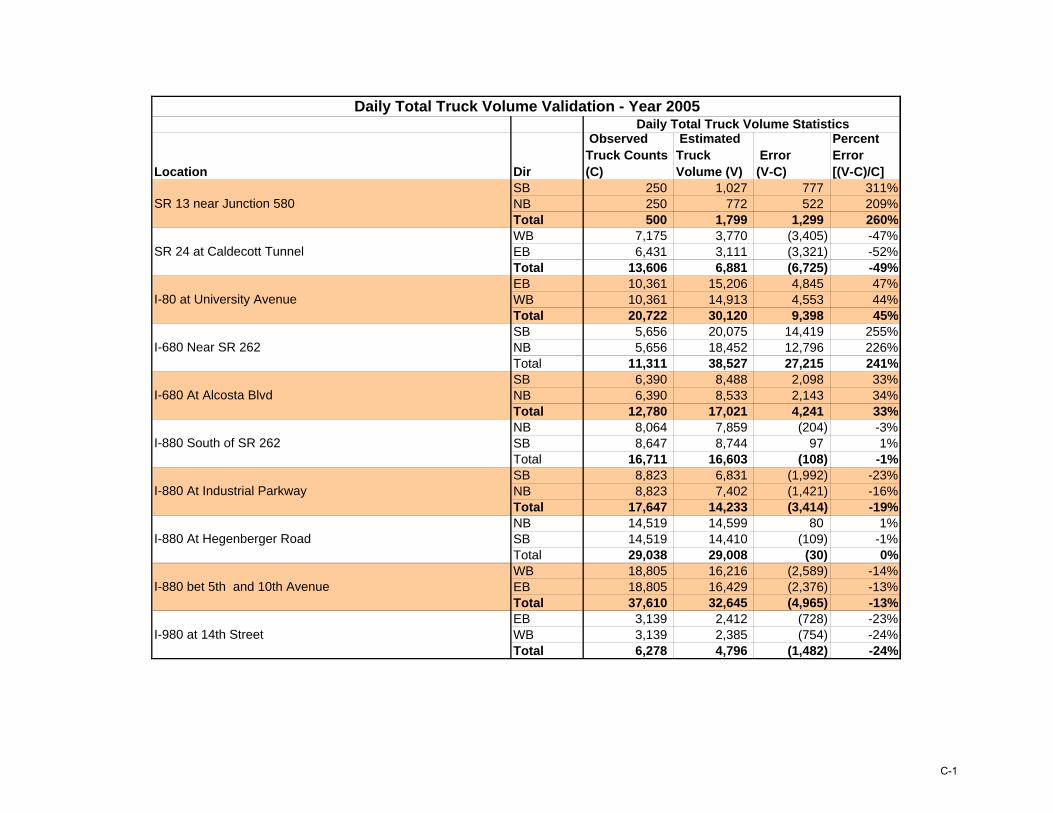
Location Dir
Observed Truck Counts (C)
Estimated Truck Volume (V)
Error (V-C)
Percent Error [(V-C)/C]
SB 250 1,027 777 311%NB 250 772 522 209%Total 500 1,799 1,299 260%WB 7,175 3,770 (3,405) -47%EB 6,431 3,111 (3,321) -52%Total 13,606 6,881 (6,725) -49%EB 10,361 15,206 4,845 47%WB 10,361 14,913 4,553 44%Total 20,722 30,120 9,398 45%SB 5,656 20,075 14,419 255%NB 5,656 18,452 12,796 226%Total 11,311 38,527 27,215 241%SB 6,390 8,488 2,098 33%NB 6,390 8,533 2,143 34%Total 12,780 17,021 4,241 33%NB 8,064 7,859 (204) -3%SB 8,647 8,744 97 1%Total 16,711 16,603 (108) -1%SB 8,823 6,831 (1,992) -23%NB 8,823 7,402 (1,421) -16%Total 17,647 14,233 (3,414) -19%NB 14,519 14,599 80 1%SB 14,519 14,410 (109) -1%Total 29,038 29,008 (30) 0%WB 18,805 16,216 (2,589) -14%EB 18,805 16,429 (2,376) -13%Total 37,610 32,645 (4,965) -13%EB 3,139 2,412 (728) -23%WB 3,139 2,385 (754) -24%Total 6,278 4,796 (1,482) -24%
Daily Total Truck Volume Statistics
I-880 At Hegenberger Road
I-880 bet 5th and 10th Avenue
I-980 at 14th Street
I-680 Near SR 262
I-680 At Alcosta Blvd
I-880 South of SR 262
I-880 At Industrial Parkway
Daily Total Truck Volume Validation - Year 2005
SR 13 near Junction 580
SR 24 at Caldecott Tunnel
I-80 at University Avenue
C-1
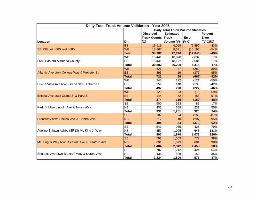
Location Dir
Observed Truck Counts (C)
Estimated Truck Volume (V)
Error (V-C)
Percent Error [(V-C)/C]
Daily Total Truck Volume StatisticsDaily Total Truck Volume Validation - Year 2005
EB 15,919 9,069 (6,850) -43%WB 18,867 8,671 (10,196) -54%Total 34,787 17,740 (17,046) -49%WB 15,441 18,078 2,637 17%EB 15,441 18,122 2,681 17%Total 30,882 36,200 5,318 17%WB 326 37 (289) -89%EB 395 19 (376) -95%Total 721 56 (665) -92%WB 243 122 (121) -50%EB 254 148 (106) -42%Total 497 270 (227) -46%WB 129 53 (76) -59%EB 144 62 (83) -57%Total 274 115 (159) -58%SB 500 583 83 17%NB 432 669 237 55%Total 931 1,251 320 34%SB 187 24 (163) -87%NB 217 10 (207) -95%Total 404 34 (370) -92%SB 541 965 425 79%NB 357 1,005 648 181%Total 897 1,970 1,073 120%SB 792 1,569 777 98%NB 691 1,373 681 98%Total 1,484 2,942 1,458 98%SB 787 1,212 424 54%NB 436 588 152 35%Total 1,224 1,800 576 47%
Shattuck Ave btwn Bancroft Way & Durant Ave
Park St btwn Lincoln Ave & Times Way
Broadway btwn Encinal Ave & Central Ave
Adeline St btwn Ashby (SR13) ML King Jr Way
ML King Jr Way btwn Alcatraz Ave & Stanford Ave
I-580 Eastern Alameda County
Atlantic Ave btwn College Way & Webster St
Buena Vista Ave btwn Grand St & Hibbard St
Encinal Ave btwn Grand St & Paru St
SR 238 bet I-880 and I-580
C-2

Location Dir
Observed Truck Counts (C)
Estimated Truck Volume (V)
Error (V-C)
Percent Error [(V-C)/C]
Daily Total Truck Volume StatisticsDaily Total Truck Volume Validation - Year 2005
WB 1,123 1,240 117 10%EB 793 553 (240) -30%Total 1,916 1,793 (123) -6%WB 863 1,157 295 34%EB 824 1,162 338 41%Total 1,686 2,319 633 38%SB 792 727 (65) -8%NB 773 1,355 583 75%Total 1,565 2,083 518 33%WB 469 343 (127) -27%EB 469 387 (83) -18%Total 939 729 (210) -22%SB 843 539 (305) -36%NB 1,064 766 (298) -28%Total 1,908 1,305 (603) -32%SB 741 126 (615) -83%NB 700 158 (542) -77%Total 1,441 284 (1,157) -80%SB 840 285 (555) -66%NB 1,018 268 (749) -74%Total 1,858 553 (1,304) -70%WB 562 253 (308) -55%EB 582 165 (417) -72%Total 1,143 418 (725) -63%SB 876 381 (495) -56%NB 1,200 396 (805) -67%Total 2,077 777 (1,300) -63%SB 714 806 92 13%NB 920 1,158 237 26%Total 1,634 1,963 329 20%
A' Street btwn Mission Blvd (SR185) & Watkins St
Clawiter Rd btwn Industrial Blvd & West St
Hesperian Blvd btwn Hollow Ave & SR 92 Ramps
Ardenwood Blvd btwn Ardenwood Terr & Kaiser Dr
Decoto Rd btwn Cabrillo Dr & I-880 Ramps
Decoto Rd btwn 7th St & 8th St
Mowry Ave btwn Fremont Blvd & Bell St
University Ave btwn 5th St & 6th St
University Ave btwn ML King Jr Way & Grant St
Herperian Blvd btwn Hacienda Ave & Bockman Rd
C-3
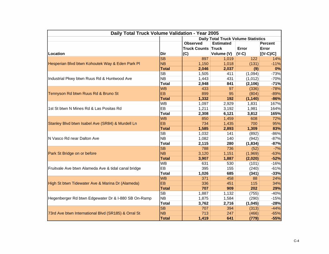
Location Dir
Observed Truck Counts (C)
Estimated Truck Volume (V)
Error (V-C)
Percent Error [(V-C)/C]
Daily Total Truck Volume StatisticsDaily Total Truck Volume Validation - Year 2005
SB 897 1,019 122 14%NB 1,150 1,018 (131) -11%Total 2,046 2,037 (9) 0%SB 1,505 411 (1,094) -73%NB 1,443 431 (1,012) -70%Total 2,948 841 (2,106) -71%WB 433 97 (336) -78%EB 899 95 (804) -89%Total 1,332 192 (1,140) -86%WB 1,097 2,929 1,831 167%EB 1,211 3,192 1,981 164%Total 2,308 6,121 3,812 165%WB 850 1,459 608 72%EB 734 1,435 700 95%Total 1,585 2,893 1,309 83%SB 1,032 141 (892) -86%NB 1,082 140 (942) -87%Total 2,115 280 (1,834) -87%SB 788 736 (52) -7%NB 3,120 1,151 (1,969) -63%Total 3,907 1,887 (2,020) -52%WB 631 530 (101) -16%EB 395 155 (240) -61%Total 1,026 685 (341) -33%WB 371 458 88 24%EB 336 451 115 34%Total 707 909 202 29%SB 1,887 1,132 (755) -40%NB 1,875 1,584 (290) -15%Total 3,762 2,716 (1,045) -28%SB 707 394 (313) -44%NB 713 247 (466) -65%Total 1,419 641 (779) -55%
Hegenberger Rd btwn Edgewater Dr & I-880 SB On-Ramp
73rd Ave btwn International Blvd (SR185) & Orral St
N Vasco Rd near Dalton Ave
Park St Bridge on or before
Fruitvale Ave btwn Alameda Ave & tidal canal bridge
High St btwn Tidewater Ave & Marina Dr (Alameda)
Industrial Pkwy btwn Ruus Rd & Huntwood Ave
Tennyson Rd btwn Ruus Rd & Bruno St
1st St btwn N Mines Rd & Las Positas Rd
Stanley Blvd btwn Isabel Ave (SR84) & Murdell Ln
Hesperian Blvd btwn Kohoutek Way & Eden Park Pl
C-4

Location Dir
Observed Truck Counts (C)
Estimated Truck Volume (V)
Error (V-C)
Percent Error [(V-C)/C]
Daily Total Truck Volume StatisticsDaily Total Truck Volume Validation - Year 2005
WB 1,029 153 (876) -85%EB 1,005 190 (815) -81%Total 2,034 343 (1,691) -83%WB 178 165 (13) -7%EB 177 270 94 53%Total 355 435 81 23%SB 307 218 (89) -29%NB 362 207 (156) -43%Total 669 425 (244) -36%WB 648 198 (450) -69%EB 431 142 (289) -67%Total 1,079 340 (739) -68%SB 1,018 616 (402) -39%NB 766 387 (379) -49%Total 1,784 1,003 (781) -44%WB 1,053 619 (434) -41%EB 1,122 953 (168) -15%Total 2,175 1,572 (602) -28%SB 448 217 (231) -52%NB 512 231 (281) -55%Total 960 448 (512) -53%SB 1,177 148 (1,029) -87%NB 1,217 355 (861) -71%Total 2,393 503 (1,890) -79%SB 745 143 (602) -81%NB 755 130 (625) -83%Total 1,500 273 (1,227) -82%SB 543 178 (364) -67%NB 539 177 (361) -67%Total 1,081 355 (726) -67%SB 636 135 (501) -79%NB 813 102 (710) -87%Total 1,449 237 (1,211) -84%
SR 61 (Doolittle Dr) btwn Swan Way & Langley St
SR 61 (Doolittle Dr) btwn Davis St & Eden Rd
SR 84 (Thornton Ave) btwn Dutra Way & Dondero Way
SR 84 (Mowry Ave) btwn Mission Blvd (SR238) & Thane St
SR 84 (Niles Canyon Rd) btwn Mission Blvd (SR238) & Old Canyon Rd
150th Ave btwn Lark St & E 14th St (SR 185)
Lewelling Blvd btwn Washington Ave & Woodgate Dr
Hesperian Blvd btwn I-238 & Springlake Dr
SR 13 (Ashby Ave) btwn 7th St & UPRR tracks (overhead)
San Leandro St btwn 77th Ave & 81st Ave
W MacArthur Blvd btwn Market St & Linden St
C-5

Location Dir
Observed Truck Counts (C)
Estimated Truck Volume (V)
Error (V-C)
Percent Error [(V-C)/C]
Daily Total Truck Volume StatisticsDaily Total Truck Volume Validation - Year 2005
SB 738 228 (510) -69%NB 672 139 (533) -79%Total 1,410 366 (1,044) -74%WB 674 83 (590) -88%EB 620 109 (511) -82%Total 1,294 193 (1,101) -85%WB 956 147 (809) -85%EB 710 193 (518) -73%Total 1,666 340 (1,326) -80%SB 1,603 1,182 (421) -26%NB 1,507 1,138 (369) -24%Total 3,110 2,320 (790) -25%WB 1,954 4,876 2,923 150%EB 2,163 5,908 3,746 173%Total 4,116 10,785 6,668 162%SB 1,404 2,182 778 55%NB 1,276 2,334 1,057 83%Total 2,680 4,516 1,835 68%WB 2,998 2,479 (520) -17%EB 2,586 2,343 (243) -9%Total 5,584 4,822 (763) -14%SB 1,409 766 (643) -46%NB 1,662 750 (912) -55%Total 3,071 1,516 (1,555) -51%WB 1,891 1,642 (250) -13%EB 2,115 1,407 (707) -33%Total 4,006 3,049 (957) -24%SB 926 137 (789) -85%NB 860 282 (578) -67%Total 1,786 419 (1,366) -77%
321,828 319,699 (2,130) -1%
98th Ave btwn I-880 & Empire
Doolittle Dr btwn Adams & Airport Dr
GRAND TOTAL
SR 262 (Mission Blvd) btwn Kato Rd/Warren Ave & Warm Springs Blvd
Martime St south of Grand Ave
7th St west of I-880
Middle Harbor Rd south of 3rd St
SR 84 (Airway Blvd) btwn Club House Dr & Kitty Hawk Rd
SR 185 (International Blvd) btwn Miller Ave & 23rd Ave
SR 185 (E 14th St) btwn Hesperian Ave & 148th Ave
SR 260 Tube Portal
C-6
AM and PM 1 - Hour Truck Volume
Validation - Year 2005

Location Dir
Observed Truck Counts (C)
Estimated Truck Volume (V)
Error (V-C)
Percent Error [(V-C)/C]
Observed Truck Counts (C)
Estimated Truck Volume (V)
Error (V-C)
Percent Error [(V-C)/C]
SB 22 39 16 73% 22 35 13 62%NB 27 26 (1) -5% 22 26 4 19%Total 49 64 15 30% 43 61 17 40%WB 493 188 (305) -62% 356 214 (141) -40%EB 291 128 (163) -56% 493 87 (406) -82%Total 784 317 (467) -60% 848 301 (547) -65%EB 631 1,147 516 82% 505 715 211 42%WB 631 753 122 19% 505 1,081 576 114%Total 1,262 1,900 638 51% 1,009 1,796 787 78%SB 480 914 434 90% 365 1,532 1,167 319%NB 480 1,927 1,447 302% 365 831 466 127%Total 960 2,841 1,881 196% 731 2,363 1,632 223%SB 480 441 (39) -8% 452 518 66 15%NB 480 744 264 55% 452 509 57 13%Total 960 1,184 224 23% 904 1,027 123 14%NB 448 431 (17) -4% 639 387 (252) -39%SB 671 520 (152) -23% 543 506 (37) -7%Total 1,119 951 (168) -15% 1,183 893 (289) -24%SB 527 383 (144) -27% 534 350 (184) -34%NB 506 397 (109) -22% 432 250 (182) -42%Total 1,033 779 (253) -25% 966 601 (365) -38%NB 642 562 (80) -12% 887 754 (133) -15%SB 942 812 (129) -14% 919 564 (355) -39%Total 1,584 1,375 (210) -13% 1,807 1,318 (489) -27%WB 943 730 (212) -23% 925 938 13 1%EB 1,095 1,033 (61) -6% 1,151 797 (354) -31%Total 2,037 1,764 (274) -13% 2,076 1,735 (341) -16%EB 185 62 (123) -67% 269 86 (182) -68%WB 266 120 (146) -55% 163 68 (95) -58%Total 451 181 (270) -60% 431 154 (277) -64%
AM - 1hr Total Truck Volume Statistics
I-880 At Hegenberger Road
I-880 bet 5th and 10th Avenue
I-980 at 14th Street
I-680 Near SR 262
I-680 At Alcosta Blvd
I-880 South of SR 262
I-880 At Industrial Parkway
AM 1-hour and PM 1-hour Truck Volume Validation - Year 2005
SR 13 near Junction 580
SR 24 at Caldecott Tunnel
I-80 at University Avenue
PM - 1hr Total Truck Volume Statistics
C-7

Location Dir
Observed Truck Counts (C)
Estimated Truck Volume (V)
Error (V-C)
Percent Error [(V-C)/C]
Observed Truck Counts (C)
Estimated Truck Volume (V)
Error (V-C)
Percent Error [(V-C)/C]
AM - 1hr Total Truck Volume Statistics
AM 1-hour and PM 1-hour Truck Volume Validation - Year 2005PM - 1hr Total Truck Volume Statistics
EB 854 498 (356) -42% 957 287 (670) -70%WB 970 309 (662) -68% 1,190 575 (615) -52%Total 1,825 807 (1,018) -56% 2,147 862 (1,285) -60%WB 816 864 48 6% 898 1,271 373 42%EB 816 1,277 461 56% 898 863 (35) -4%Total 1,633 2,141 508 31% 1,796 2,134 338 19%WB 26 14 (13) -48% 19 2 (17) -92%EB 24 10 (14) -58% 25 8 (16) -67%Total 50 24 (26) -53% 43 10 (34) -78%WB 30 12 (18) -60% 8 11 3 36%EB 14 12 (2) -15% 15 12 (2) -16%Total 45 24 (20) -45% 23 24 1 3%WB 16 6 (11) -65% 4 6 2 40%EB 10 7 (4) -37% 14 9 (5) -39%Total 27 12 (14) -54% 19 15 (4) -20%SB 29 22 (7) -25% 26 32 5 21%NB 22 40 18 80% 18 26 8 48%Total 51 62 10 20% 44 58 14 32%SB 10 1 (9) -88% 17 1 (16) -93%NB 14 1 (12) -91% 15 1 (14) -93%Total 24 2 (21) -90% 32 2 (30) -93%SB 24 81 57 239% 42 51 8 20%NB 27 64 36 133% 23 46 22 97%Total 51 145 94 183% 66 96 31 47%SB 42 124 82 195% 61 92 30 50%NB 53 90 37 69% 54 78 24 44%Total 95 214 119 125% 115 169 54 47%SB 48 106 57 119% 43 63 20 46%NB 40 30 (10) -25% 19 16 (4) -19%Total 88 135 47 54% 62 78 16 26%
Shattuck Ave btwn Bancroft Way & Durant Ave
Park St btwn Lincoln Ave & Times Way
Broadway btwn Encinal Ave & Central Ave
Adeline St btwn Ashby (SR13) ML King Jr Way
ML King Jr Way btwn Alcatraz Ave & Stanford Ave
I-580 Eastern Alameda County
Atlantic Ave btwn College Way & Webster St
Buena Vista Ave btwn Grand St & Hibbard St
Encinal Ave btwn Grand St & Paru St
SR 238 bet I-880 and I-580
C-8

Location Dir
Observed Truck Counts (C)
Estimated Truck Volume (V)
Error (V-C)
Percent Error [(V-C)/C]
Observed Truck Counts (C)
Estimated Truck Volume (V)
Error (V-C)
Percent Error [(V-C)/C]
AM - 1hr Total Truck Volume Statistics
AM 1-hour and PM 1-hour Truck Volume Validation - Year 2005PM - 1hr Total Truck Volume Statistics
WB 78 117 39 51% 55 67 13 24%EB 71 24 (47) -66% 27 37 10 36%Total 148 141 (8) -5% 81 104 23 28%WB 47 115 68 147% 50 75 25 49%EB 60 95 35 58% 43 95 51 119%Total 107 209 103 97% 94 170 76 81%SB 70 76 5 7% 51 52 2 3%NB 46 63 17 36% 58 116 58 100%Total 116 138 22 19% 109 169 60 55%WB 27 17 (9) -35% 63 49 (14) -22%EB 46 47 1 3% 40 29 (10) -26%Total 72 64 (8) -11% 103 79 (24) -23%SB 66 37 (29) -44% 17 74 57 331%NB 48 47 (2) -3% 75 70 (5) -6%Total 114 83 (31) -27% 92 144 52 56%SB 71 34 (37) -51% 42 8 (34) -82%NB 41 7 (34) -83% 62 15 (46) -75%Total 112 41 (70) -63% 103 23 (81) -78%SB 43 21 (23) -52% 53 20 (33) -63%NB 64 17 (47) -73% 66 29 (37) -56%Total 107 38 (69) -65% 119 49 (70) -59%WB 42 23 (20) -46% 37 5 (32) -86%EB 34 3 (31) -90% 50 32 (18) -36%Total 76 26 (50) -66% 87 37 (50) -58%SB 104 22 (81) -78% 52 42 (10) -19%NB 80 35 (45) -56% 84 53 (31) -37%Total 184 57 (127) -69% 135 95 (41) -30%SB 44 87 42 96% 48 70 22 46%NB 78 67 (12) -15% 66 69 3 4%Total 123 154 31 25% 114 139 25 22%
A' Street btwn Mission Blvd (SR185) & Watkins St
Clawiter Rd btwn Industrial Blvd & West St
Hesperian Blvd btwn Hollow Ave & SR 92 Ramps
Ardenwood Blvd btwn Ardenwood Terr & Kaiser Dr
Decoto Rd btwn Cabrillo Dr & I-880 Ramps
Decoto Rd btwn 7th St & 8th St
Mowry Ave btwn Fremont Blvd & Bell St
University Ave btwn 5th St & 6th St
University Ave btwn ML King Jr Way & Grant St
Herperian Blvd btwn Hacienda Ave & Bockman Rd
C-9

Location Dir
Observed Truck Counts (C)
Estimated Truck Volume (V)
Error (V-C)
Percent Error [(V-C)/C]
Observed Truck Counts (C)
Estimated Truck Volume (V)
Error (V-C)
Percent Error [(V-C)/C]
AM - 1hr Total Truck Volume Statistics
AM 1-hour and PM 1-hour Truck Volume Validation - Year 2005PM - 1hr Total Truck Volume Statistics
SB 65 146 82 126% 72 81 10 13%NB 101 50 (52) -51% 77 81 5 6%Total 166 196 30 18% 149 163 14 10%SB 115 23 (92) -80% 63 30 (33) -53%NB 88 27 (62) -70% 101 24 (77) -76%Total 204 50 (154) -75% 164 54 (110) -67%WB 40 10 (29) -74% 27 5 (22) -82%EB 60 4 (56) -94% 67 12 (56) -83%Total 99 14 (85) -86% 95 16 (78) -83%WB 99 183 84 85% 49 411 362 739%EB 53 427 375 711% 85 226 141 166%Total 152 610 459 303% 134 638 504 376%WB 144 183 39 27% 14 283 269 1962%EB 27 247 220 802% 96 199 103 107%Total 172 430 258 150% 110 482 372 339%SB 102 4 (98) -96% 32 7 (24) -78%NB 60 13 (47) -79% 90 4 (85) -95%Total 162 17 (145) -90% 121 11 (110) -91%SB 39 34 (5) -14% 46 42 (4) -9%NB 57 66 9 17% 281 42 (239) -85%Total 96 100 4 4% 326 84 (243) -74%WB 49 25 (24) -50% 42 35 (6) -15%EB 30 22 (8) -27% 25 16 (9) -37%Total 79 47 (32) -41% 67 51 (16) -23%WB 27 28 1 3% 28 19 (9) -31%EB 24 24 (1) -2% 21 31 10 45%Total 51 51 0 0% 49 50 1 2%SB 109 114 6 5% 108 139 31 29%NB 117 145 27 23% 105 139 33 32%Total 226 259 33 15% 213 278 64 30%
Hegenberger Rd btwn Edgewater Dr & I-880 SB On-Ramp
N Vasco Rd near Dalton Ave
Park St Bridge on or before
Fruitvale Ave btwn Alameda Ave & tidal canal bridge
High St btwn Tidewater Ave & Marina Dr (Alameda)
Industrial Pkwy btwn Ruus Rd & Huntwood Ave
Tennyson Rd btwn Ruus Rd & Bruno St
1st St btwn N Mines Rd & Las Positas Rd
Stanley Blvd btwn Isabel Ave (SR84) & Murdell Ln
Hesperian Blvd btwn Kohoutek Way & Eden Park Pl
C-10

Location Dir
Observed Truck Counts (C)
Estimated Truck Volume (V)
Error (V-C)
Percent Error [(V-C)/C]
Observed Truck Counts (C)
Estimated Truck Volume (V)
Error (V-C)
Percent Error [(V-C)/C]
AM - 1hr Total Truck Volume Statistics
AM 1-hour and PM 1-hour Truck Volume Validation - Year 2005PM - 1hr Total Truck Volume Statistics
SB 57 25 (32) -56% 43 26 (17) -39%NB 45 21 (24) -54% 46 24 (22) -48%Total 103 46 (56) -55% 90 51 (39) -44%WB 65 24 (41) -64% 84 26 (59) -70%EB 51 19 (32) -63% 81 46 (35) -43%Total 116 43 (74) -63% 165 72 (94) -57%WB 12 11 (1) -5% 15 16 1 7%EB 12 18 6 55% 15 17 2 12%Total 23 29 6 25% 30 33 3 9%SB 15 8 (7) -49% 26 10 (16) -62%NB 24 10 (14) -60% 36 12 (24) -66%Total 39 17 (21) -55% 61 22 (39) -64%WB 41 15 (26) -63% 49 5 (44) -91%EB 38 3 (36) -93% 29 13 (15) -53%Total 80 18 (62) -78% 78 18 (60) -77%SB 71 19 (52) -74% 66 35 (31) -47%NB 62 22 (41) -65% 56 13 (43) -77%Total 133 40 (93) -70% 122 48 (74) -61%WB 57 50 (6) -11% 68 36 (32) -47%EB 79 39 (39) -50% 45 104 58 128%Total 135 90 (45) -34% 114 140 26 23%SB 24 23 (2) -7% 31 27 (4) -14%NB 38 23 (16) -41% 31 26 (5) -15%Total 62 45 (17) -28% 62 53 (9) -14%SB 59 25 (33) -57% 86 112 26 31%NB 67 76 9 13% 60 78 17 29%Total 126 102 (24) -19% 146 190 44 30%SB 63 19 (44) -70% 38 12 (27) -70%NB 52 7 (44) -86% 41 17 (25) -60%Total 115 26 (88) -77% 80 28 (52) -65%
SR 61 (Doolittle Dr) btwn Swan Way & Langley St
SR 61 (Doolittle Dr) btwn Davis St & Eden Rd
SR 84 (Thornton Ave) btwn Dutra Way & Dondero Way
150th Ave btwn Lark St & E 14th St (SR 185)
Lewelling Blvd btwn Washington Ave & Woodgate Dr
Hesperian Blvd btwn I-238 & Springlake Dr
SR 13 (Ashby Ave) btwn 7th St & UPRR tracks (overhead)
73rd Ave btwn International Blvd (SR185) & Orral St
San Leandro St btwn 77th Ave & 81st Ave
W MacArthur Blvd btwn Market St & Linden St
C-11

Location Dir
Observed Truck Counts (C)
Estimated Truck Volume (V)
Error (V-C)
Percent Error [(V-C)/C]
Observed Truck Counts (C)
Estimated Truck Volume (V)
Error (V-C)
Percent Error [(V-C)/C]
AM - 1hr Total Truck Volume Statistics
AM 1-hour and PM 1-hour Truck Volume Validation - Year 2005PM - 1hr Total Truck Volume Statistics
SB 46 19 (27) -59% 28 10 (18) -64%NB 31 9 (21) -70% 35 16 (20) -55%Total 77 28 (49) -63% 63 26 (38) -59%SB 70 174 104 148% 42 41 (1) -3%NB 54 17 (37) -69% 65 129 64 98%Total 124 191 67 54% 107 170 63 59%SB 48 13 (35) -73% 47 12 (35) -74%NB 37 22 (15) -40% 40 11 (29) -73%Total 85 35 (50) -59% 87 23 (64) -73%WB 47 9 (38) -82% 39 12 (27) -70%EB 26 7 (19) -74% 42 27 (15) -36%Total 72 15 (57) -79% 81 39 (42) -52%WB 54 9 (45) -84% 65 7 (58) -90%EB 37 8 (29) -78% 54 23 (31) -57%Total 91 17 (74) -81% 119 30 (89) -75%SB 105 63 (43) -40% 136 109 (28) -20%NB 108 87 (21) -20% 86 71 (15) -17%Total 214 150 (64) -30% 222 179 (42) -19%WB 90 212 122 135% 57 516 459 803%EB 91 788 697 768% 82 254 172 209%Total 181 1,000 820 453% 139 770 630 453%SB 99 222 123 124% 45 236 191 426%NB 92 185 93 101% 83 197 114 136%Total 191 407 216 113% 128 433 305 237%WB 259 167 (93) -36% 95 178 83 87%EB 155 189 34 22% 211 196 (15) -7%Total 415 356 (59) -14% 306 374 68 22%SB 118 57 (61) -52% 30 62 33 109%NB 139 56 (84) -60% 137 59 (78) -57%Total 258 113 (145) -56% 167 121 (46) -27%WB 109 77 (31) -29% 92 90 (2) -3%EB 87 89 2 3% 86 56 (30) -35%Total 195 166 (29) -15% 178 146 (32) -18%SB 50 20 (30) -61% 76 105 30 39%NB 58 70 12 20% 45 71 26 57%Total 108 90 (19) -17% 121 177 56 46%
19,635 20,672 1,036 5% 19,479 19,675 196 1%
98th Ave btwn I-880 & Empire
Doolittle Dr btwn Adams & Airport Dr
GRAND TOTAL
SR 262 (Mission Blvd) btwn Kato Rd/Warren Ave & Warm Springs Blvd
Martime St south of Grand Ave
7th St west of I-880
Middle Harbor Rd south of 3rd St
SR 84 (Airway Blvd) btwn Club House Dr & Kitty Hawk Rd
SR 185 (International Blvd) btwn Miller Ave & 23rd Ave
SR 185 (E 14th St) btwn Hesperian Ave & 148th Ave
SR 260 Tube Portal
SR 84 (Mowry Ave) btwn Mission Blvd (SR238) & Thane St
SR 84 (Niles Canyon Rd) btwn Mission Blvd (SR238) & Old Canyon Rd
C-12

PM 2 and 4 Hour Truck Volume
Validation – Year 2005
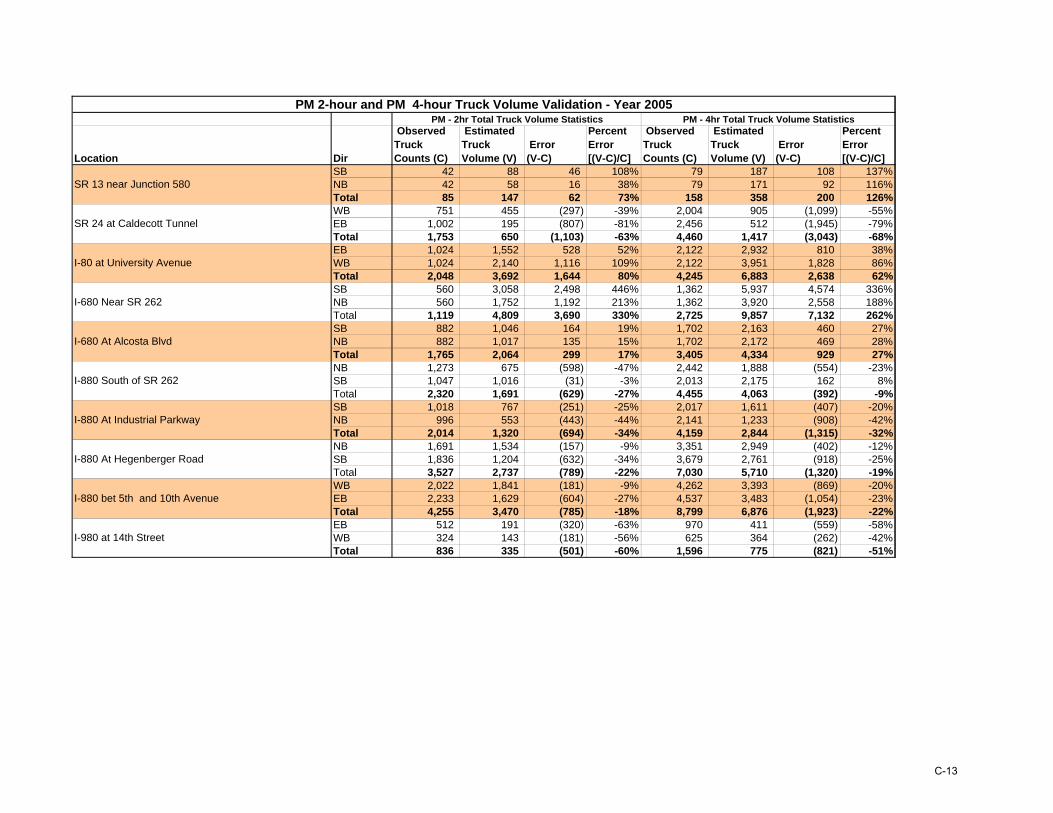
Location Dir
Observed Truck Counts (C)
Estimated Truck Volume (V)
Error (V-C)
Percent Error [(V-C)/C]
Observed Truck Counts (C)
Estimated Truck Volume (V)
Error (V-C)
Percent Error [(V-C)/C]
SB 42 88 46 108% 79 187 108 137%NB 42 58 16 38% 79 171 92 116%Total 85 147 62 73% 158 358 200 126%WB 751 455 (297) -39% 2,004 905 (1,099) -55%EB 1,002 195 (807) -81% 2,456 512 (1,945) -79%Total 1,753 650 (1,103) -63% 4,460 1,417 (3,043) -68%EB 1,024 1,552 528 52% 2,122 2,932 810 38%WB 1,024 2,140 1,116 109% 2,122 3,951 1,828 86%Total 2,048 3,692 1,644 80% 4,245 6,883 2,638 62%SB 560 3,058 2,498 446% 1,362 5,937 4,574 336%NB 560 1,752 1,192 213% 1,362 3,920 2,558 188%Total 1,119 4,809 3,690 330% 2,725 9,857 7,132 262%SB 882 1,046 164 19% 1,702 2,163 460 27%NB 882 1,017 135 15% 1,702 2,172 469 28%Total 1,765 2,064 299 17% 3,405 4,334 929 27%NB 1,273 675 (598) -47% 2,442 1,888 (554) -23%SB 1,047 1,016 (31) -3% 2,013 2,175 162 8%Total 2,320 1,691 (629) -27% 4,455 4,063 (392) -9%SB 1,018 767 (251) -25% 2,017 1,611 (407) -20%NB 996 553 (443) -44% 2,141 1,233 (908) -42%Total 2,014 1,320 (694) -34% 4,159 2,844 (1,315) -32%NB 1,691 1,534 (157) -9% 3,351 2,949 (402) -12%SB 1,836 1,204 (632) -34% 3,679 2,761 (918) -25%Total 3,527 2,737 (789) -22% 7,030 5,710 (1,320) -19%WB 2,022 1,841 (181) -9% 4,262 3,393 (869) -20%EB 2,233 1,629 (604) -27% 4,537 3,483 (1,054) -23%Total 4,255 3,470 (785) -18% 8,799 6,876 (1,923) -22%EB 512 191 (320) -63% 970 411 (559) -58%WB 324 143 (181) -56% 625 364 (262) -42%Total 836 335 (501) -60% 1,596 775 (821) -51%
PM - 2hr Total Truck Volume Statistics
I-880 At Hegenberger Road
I-880 bet 5th and 10th Avenue
I-980 at 14th Street
I-680 Near SR 262
I-680 At Alcosta Blvd
I-880 South of SR 262
I-880 At Industrial Parkway
PM 2-hour and PM 4-hour Truck Volume Validation - Year 2005
SR 13 near Junction 580
SR 24 at Caldecott Tunnel
I-80 at University Avenue
PM - 4hr Total Truck Volume Statistics
C-13
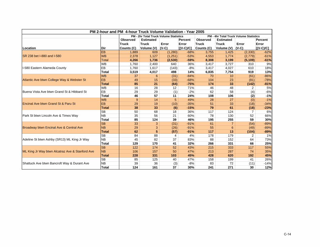
Location Dir
Observed Truck Counts (C)
Estimated Truck Volume (V)
Error (V-C)
Percent Error [(V-C)/C]
Observed Truck Counts (C)
Estimated Truck Volume (V)
Error (V-C)
Percent Error [(V-C)/C]
PM - 2hr Total Truck Volume Statistics
PM 2-hour and PM 4-hour Truck Volume Validation - Year 2005PM - 4hr Total Truck Volume Statistics
EB 1,889 609 (1,280) -68% 3,755 1,425 (2,330) -62%WB 2,378 1,127 (1,251) -53% 4,553 1,774 (2,779) -61%Total 4,266 1,736 (2,530) -59% 8,308 3,199 (5,109) -61%WB 1,760 2,400 640 36% 3,417 3,727 310 9%EB 1,760 1,617 (143) -8% 3,417 4,027 610 18%Total 3,519 4,017 498 14% 6,835 7,754 919 13%WB 37 6 (31) -84% 70 10 (61) -86%EB 49 15 (33) -68% 104 23 (81) -78%Total 85 21 (64) -75% 174 33 (142) -81%WB 16 28 12 71% 46 48 2 5%EB 29 29 (1) -2% 62 58 (4) -6%Total 46 57 11 24% 108 106 (2) -1%WB 9 14 5 49% 28 27 (0) -1%EB 29 19 (10) -35% 51 33 (18) -34%Total 38 33 (6) -15% 79 61 (18) -23%SB 50 68 18 36% 117 124 7 6%NB 35 56 21 60% 78 130 52 66%Total 85 124 39 46% 195 255 59 30%SB 33 3 (31) -91% 61 7 (54) -89%NB 29 3 (26) -91% 55 6 (49) -89%Total 62 5 (57) -91% 117 13 (104) -89%SB 84 88 4 4% 178 179 2 1%NB 45 82 37 83% 88 152 64 73%Total 129 170 41 32% 266 331 66 25%SB 122 174 52 43% 215 333 117 55%NB 106 157 50 47% 213 287 74 35%Total 228 331 103 45% 428 620 192 45%SB 85 125 40 47% 158 199 41 26%NB 39 36 (3) -8% 83 72 (11) -14%Total 124 161 37 30% 241 271 30 12%
Shattuck Ave btwn Bancroft Way & Durant Ave
Park St btwn Lincoln Ave & Times Way
Broadway btwn Encinal Ave & Central Ave
Adeline St btwn Ashby (SR13) ML King Jr Way
ML King Jr Way btwn Alcatraz Ave & Stanford Ave
I-580 Eastern Alameda County
Atlantic Ave btwn College Way & Webster St
Buena Vista Ave btwn Grand St & Hibbard St
Encinal Ave btwn Grand St & Paru St
SR 238 bet I-880 and I-580
C-14

Location Dir
Observed Truck Counts (C)
Estimated Truck Volume (V)
Error (V-C)
Percent Error [(V-C)/C]
Observed Truck Counts (C)
Estimated Truck Volume (V)
Error (V-C)
Percent Error [(V-C)/C]
PM - 2hr Total Truck Volume Statistics
PM 2-hour and PM 4-hour Truck Volume Validation - Year 2005PM - 4hr Total Truck Volume Statistics
WB 109 158 49 45% 220 286 66 30%EB 53 77 24 46% 111 139 28 25%Total 161 235 74 46% 331 424 93 28%WB 98 141 43 44% 219 237 18 8%EB 88 171 83 95% 155 250 95 62%Total 186 312 126 68% 374 487 113 30%SB 101 97 (4) -4% 187 297 110 59%NB 116 192 76 66% 214 538 324 152%Total 217 289 72 33% 401 834 434 108%WB 126 73 (53) -42% 211 175 (36) -17%EB 78 51 (27) -35% 133 126 (7) -5%Total 203 124 (80) -39% 344 300 (44) -13%SB 34 149 115 341% 74 274 200 270%NB 151 158 7 5% 295 330 35 12%Total 184 307 122 66% 369 604 235 64%SB 84 18 (66) -79% 165 36 (130) -78%NB 123 12 (111) -90% 219 72 (148) -67%Total 207 30 (177) -86% 385 107 (277) -72%SB 105 36 (69) -66% 208 80 (128) -62%NB 133 44 (89) -67% 276 95 (181) -66%Total 238 79 (158) -67% 484 175 (309) -64%WB 72 17 (55) -76% 144 46 (98) -68%EB 101 65 (37) -36% 175 261 86 49%Total 173 82 (92) -53% 319 307 (12) -4%SB 93 79 (14) -16% 154 188 35 22%NB 183 70 (113) -62% 343 317 (26) -8%Total 277 149 (127) -46% 497 505 9 2%SB 96 154 58 61% 190 335 145 77%NB 131 147 16 12% 238 329 91 38%Total 227 301 74 33% 428 664 236 55%SB 143 137 (6) -4% 243 386 143 59%NB 154 153 (1) -1% 290 370 79 27%Total 297 290 (7) -2% 533 755 222 42%SB 125 58 (67) -54% 268 112 (156) -58%NB 202 50 (152) -75% 391 101 (289) -74%Total 327 108 (219) -67% 658 214 (445) -68%WB 54 11 (43) -80% 110 47 (63) -57%EB 135 22 (113) -83% 272 75 (197) -72%Total 189 33 (156) -82% 383 122 (260) -68%WB 97 751 654 671% 200 1,183 983 493%EB 169 439 270 159% 360 997 637 177%Total 267 1,190 923 346% 559 2,180 1,620 290%
Industrial Pkwy btwn Ruus Rd & Huntwood Ave
Tennyson Rd btwn Ruus Rd & Bruno St
1st St btwn N Mines Rd & Las Positas Rd
A' Street btwn Mission Blvd (SR185) & Watkins St
Clawiter Rd btwn Industrial Blvd & West St
Hesperian Blvd btwn Hollow Ave & SR 92 Ramps
Hesperian Blvd btwn Kohoutek Way & Eden Park Pl
Ardenwood Blvd btwn Ardenwood Terr & Kaiser Dr
Decoto Rd btwn Cabrillo Dr & I-880 Ramps
Decoto Rd btwn 7th St & 8th St
Mowry Ave btwn Fremont Blvd & Bell St
University Ave btwn 5th St & 6th St
University Ave btwn ML King Jr Way & Grant St
Herperian Blvd btwn Hacienda Ave & Bockman Rd
C-15

Location Dir
Observed Truck Counts (C)
Estimated Truck Volume (V)
Error (V-C)
Percent Error [(V-C)/C]
Observed Truck Counts (C)
Estimated Truck Volume (V)
Error (V-C)
Percent Error [(V-C)/C]
PM - 2hr Total Truck Volume Statistics
PM 2-hour and PM 4-hour Truck Volume Validation - Year 2005PM - 4hr Total Truck Volume Statistics
WB 27 529 502 1883% 74 919 844 1137%EB 191 379 187 98% 329 909 580 176%Total 218 908 690 316% 404 1,828 1,424 353%SB 64 15 (48) -76% 121 38 (83) -69%NB 179 9 (170) -95% 340 23 (317) -93%Total 242 24 (218) -90% 461 61 (400) -87%SB 90 110 20 22% 184 179 (5) -3%NB 561 100 (462) -82% 1,116 233 (883) -79%Total 651 210 (442) -68% 1,299 411 (888) -68%WB 83 72 (11) -14% 144 161 16 11%EB 50 32 (18) -35% 89 89 0 0%Total 133 104 (29) -22% 233 250 17 7%WB 54 43 (12) -22% 97 87 (10) -11%EB 44 48 4 9% 83 123 40 48%Total 98 91 (8) -8% 180 210 30 16%SB 215 250 35 16% 439 416 (23) -5%NB 210 272 62 29% 422 431 9 2%Total 425 522 97 23% 860 846 (14) -2%SB 87 66 (21) -24% 165 140 (25) -15%NB 91 47 (44) -48% 196 132 (65) -33%Total 178 113 (65) -36% 362 272 (89) -25%WB 169 42 (127) -75% 309 127 (182) -59%EB 140 70 (70) -50% 260 158 (102) -39%Total 309 112 (197) -64% 569 285 (284) -50%WB 31 27 (5) -15% 51 82 31 62%EB 30 34 4 12% 61 84 23 37%Total 61 60 (1) -1% 112 166 54 48%SB 51 27 (24) -47% 93 58 (35) -37%NB 71 18 (53) -75% 119 41 (79) -66%Total 122 45 (77) -63% 213 99 (114) -53%
150th Ave btwn Lark St & E 14th St (SR 185)
Hegenberger Rd btwn Edgewater Dr & I-880 SB On-Ra
73rd Ave btwn International Blvd (SR185) & Orral St
San Leandro St btwn 77th Ave & 81st Ave
W MacArthur Blvd btwn Market St & Linden St
N Vasco Rd near Dalton Ave
Park St Bridge on or before
Fruitvale Ave btwn Alameda Ave & tidal canal bridge
High St btwn Tidewater Ave & Marina Dr (Alameda)
Stanley Blvd btwn Isabel Ave (SR84) & Murdell Ln
C-16

Location Dir
Observed Truck Counts (C)
Estimated Truck Volume (V)
Error (V-C)
Percent Error [(V-C)/C]
Observed Truck Counts (C)
Estimated Truck Volume (V)
Error (V-C)
Percent Error [(V-C)/C]
PM - 2hr Total Truck Volume Statistics
PM 2-hour and PM 4-hour Truck Volume Validation - Year 2005PM - 4hr Total Truck Volume Statistics
WB 97 16 (81) -84% 222 68 (154) -69%EB 56 25 (31) -55% 131 73 (58) -44%Total 153 41 (112) -73% 352 141 (211) -60%SB 131 76 (55) -42% 267 182 (85) -32%NB 112 36 (76) -68% 203 96 (107) -53%Total 243 112 (131) -54% 470 278 (192) -41%WB 136 73 (63) -46% 254 181 (73) -29%EB 90 193 102 114% 198 424 226 115%Total 226 266 39 17% 452 605 154 34%SB 61 60 (1) -2% 129 133 3 2%NB 62 54 (8) -13% 106 126 20 19%Total 124 114 (9) -8% 236 259 23 10%SB 171 236 65 38% 348 405 58 17%NB 121 157 36 30% 272 392 121 45%Total 292 393 101 35% 619 798 179 29%SB 76 25 (51) -67% 168 45 (122) -73%NB 81 32 (49) -60% 171 59 (113) -66%Total 158 57 (100) -64% 339 104 (235) -69%SB 55 24 (31) -56% 109 54 (55) -51%NB 70 50 (20) -29% 139 135 (4) -3%Total 125 74 (51) -41% 248 189 (59) -24%SB 85 77 (8) -10% 156 152 (4) -3%NB 130 148 18 14% 270 727 457 169%Total 215 225 10 5% 426 879 453 106%SB 73 26 (47) -64% 158 65 (93) -59%NB 81 20 (60) -75% 148 52 (96) -65%Total 153 46 (107) -70% 306 117 (189) -62%WB 78 16 (62) -80% 180 69 (111) -62%EB 82 48 (34) -42% 167 130 (38) -22%Total 160 64 (97) -60% 347 199 (149) -43%
SR 84 (Airway Blvd) btwn Club House Dr & Kitty Hawk
SR 61 (Doolittle Dr) btwn Swan Way & Langley St
SR 185 (International Blvd) btwn Miller Ave & 23rd Ave
SR 61 (Doolittle Dr) btwn Davis St & Eden Rd
SR 84 (Thornton Ave) btwn Dutra Way & Dondero Way
SR 84 (Mowry Ave) btwn Mission Blvd (SR238) & Than
SR 84 (Niles Canyon Rd) btwn Mission Blvd (SR238) &
Lewelling Blvd btwn Washington Ave & Woodgate Dr
Hesperian Blvd btwn I-238 & Springlake Dr
SR 13 (Ashby Ave) btwn 7th St & UPRR tracks (overhe
C-17

Location Dir
Observed Truck Counts (C)
Estimated Truck Volume (V)
Error (V-C)
Percent Error [(V-C)/C]
Observed Truck Counts (C)
Estimated Truck Volume (V)
Error (V-C)
Percent Error [(V-C)/C]
PM - 2hr Total Truck Volume Statistics
PM 2-hour and PM 4-hour Truck Volume Validation - Year 2005PM - 4hr Total Truck Volume Statistics
WB 129 17 (111) -86% 255 48 (207) -81%EB 106 41 (65) -61% 197 129 (68) -34%Total 235 59 (176) -75% 452 178 (274) -61%SB 271 215 (56) -21% 482 393 (89) -18%NB 170 151 (19) -11% 349 326 (23) -7%Total 441 366 (75) -17% 830 718 (112) -13%WB 115 958 843 733% 221 1,767 1,546 699%EB 164 479 315 192% 394 1,130 736 187%Total 279 1,437 1,158 415% 615 2,897 2,282 371%SB 89 415 326 366% 197 768 571 291%NB 166 347 181 109% 288 649 361 126%Total 255 761 506 198% 484 1,417 933 193%WB 191 317 127 67% 437 569 133 30%EB 422 349 (72) -17% 686 689 3 0%Total 612 667 55 9% 1,123 1,258 135 12%SB 59 110 51 87% 150 205 55 37%NB 273 105 (168) -62% 416 207 (209) -50%Total 331 215 (117) -35% 566 412 (154) -27%WB 184 179 (5) -3% 395 248 (147) -37%EB 172 102 (70) -40% 345 184 (161) -47%Total 355 281 (74) -21% 741 432 (309) -42%SB 151 221 69 46% 288 381 93 32%NB 91 143 52 57% 198 369 171 86%Total 242 363 121 50% 486 750 264 54%
38,497 38,832 335 1% 77,628 79,496 1,869 2%
98th Ave btwn I-880 & Empire
Doolittle Dr btwn Adams & Airport Dr
GRAND TOTAL
SR 262 (Mission Blvd) btwn Kato Rd/Warren Ave & Wa
Martime St south of Grand Ave
7th St west of I-880
Middle Harbor Rd south of 3rd St
SR 185 (E 14th St) btwn Hesperian Ave & 148th Ave
SR 260 Tube Portal
C-18


The Countywide Truck Travel Demand Model
Cambridge Systematics, Inc. D-1
Appendix D. Glossary
Acronym Definition of Acronym
AADT Annual Average Daily traffic
ABAG Association of Bay Area Governments
CFS Commodity Flow Survey
CS Cambridge Systematics, Inc.
CTP Countywide Transportation Plan
DOT Department of Transportation
EI-IE-EE External Internal/Internal External/External External
FAF Freight Analysis Framework
FHWA Federal Highway Administration
GVW Gross Vehicle Weight
HGAC Houston-Galveston Area Council
IE/EI Internal External/External Internal
I-O Input-output Model
LAMTA/MTA/Metro Los Angeles Metropolitan Transit Authority
MPO Mariposa Association Government
MPO Metropolitan Planning Organization
MTC Metropolitan Transportation Commission
NAICS North American Industries Classification System
NCFRP National Cooperative Freight Research Program
NCHRP National Cooperative Highway Research Program
NHI National Highway Institute
O-D table Origin-Destination table
ODME Origin Destination Matrix Estimation
PCE Passenger Car Equivalents
pcphpl passenger car per hour per lane
PeMS Performance Management System
QRFM Quick Response Freight Manual

The Countywide Truck Travel Demand Model
D-2 Cambridge Systematics, Inc.
Acronym Definition of Acronym
RMSE Root Mean Square
R-squared overall goodness of fit measure
SCAG Southern California Association of Governments
SMILE Strategic Model for Integrated Logistics Evaluation
TAZ Traffic Analysis Zone
TLFD Trip Length Frequency Distribution
TNO Inro Dutch organization for scientific research
VMT Vehicle Miles of Travel
VTA Santa Clara Valley Transportation Authority