The Cost-Sharing, Shadow Price and Cluster inMedical Care Utilization: A Self-Exciting

Perspective ∗

Yuhao LIyuli@eco.uc3m.es

This Version Jun, 2019, First Version, Aug, 2016

Departamento de Economia, Universidad Carlos III de Madrid

Abstract

In this paper, a self-exciting counting process modelling method is proposedto study the frequency of medical care service utilization under a non-linearbudget constraint health insurance policy. This modelling strategy enablesresearchers to investigate individual’s dynamic behavior in a more detailedway. Specifically, for each individual, every doctor visiting record is repre-sented as a point in a self-exciting counting process. Cost associated with suchvisiting is included in this counting process as a mark. A minimum distancemethod is employed to find the estimators. Using the Rand Health InsuranceExperiment data, we find that individuals respond to a change of shadowprice. In addition, using external models, we find that once conditional ona state-dependent structure, there is little unobserved heterogeneity effect.Lastly, we use a matured cluster analysis algorithm to investigate the clusterpatterns and discover that compared to free plan, cost-sharing insurance planwith out-of-pocket fees suppress the use of medical services by limiting thenumber of clusters as well as follow-up visiting within each cluster.

JEL. C41, C13, C51, I13, I12

Keywords. Health insurance, non-linear budget constraint, medical serviceutilization, self-exciting process, history-dependent dynamic, minimum distanceestimation

∗I am grateful to Prof.Miguel.A.Delgado for supports and guidance throughout this projectand to Prof.Winfried Stute for his inspiration and valuable comments. I would also like to thankconference and seminar participants at the EEA-ESEM Lison, the IAAE Montreal, the UC3MEconometrics workshop.

1

1 Introduction

In this paper, we aim to model individual’s doctor-visiting behavior (outpatientonly) under a non-linear cost environment using a self-exciting process. Recentstudies on health insurance (e.g., Aron-Dine et al. (2012),Einav et al. (2015)) deviatefrom the classical assumption that individuals only respond to a single linear spotcost1 and find strong evidence that individuals respond to the dynamic incentivesassociated with the non-linear nature of a typical health insurance contract. Theseconclusions suggest that ‘it is unlikely that a single elasticity estimate can summarizethe spending response to changes in health insurance’ and ’such an estimate is notconceptually well defined.’ (Aron-Dine et al., 2012).

The driving forces of such a non-linear nature are cost-sharing policies imple-mented in a health insurance contract. The most common ones are the deductible,the co-insurance rate and the out-of-pocket fee cap (OPC). In a typical setup, in-dividuals need to cover all their medical expenditures below the deductible. Oncethe threshold is passed, co-insurance is applied, where individuals pay part of theexpenditures based on the co-insurance rate. Finally, if the total expenditure paidby the individual passes the OPC, no cost (or very little cost) would be paid by thisindividual. Figure 1 illustrates such a typical non-linear budget constraint.

Total Expenditure

(Nom

inal

)In

div

idual

Cos

tX

(t)

ADeductible

BOPC

45◦

tan−1(r) < 45◦

The total expenditure is the sum of individual costs and costs paid by the insurance. Points A andB are the deductible threshold and OPC, respectively. When the total expenditure is below A, theco-insurance is 100% (individuals pay all cost) and the slope is 1. Between A and B, a co-insurancerate (the slope) 0 < r < 1 is applied. Whenever the total expenditure is beyond B, there is no costfor individuals (the slope is 0).

Figure 1: Non-linear Individual Cost (Medical Price)

At the heart of this non-linearity is the stochastic cumulative individual costX(t). Keeler, Newhouse, and Phelps (1977) is the first theoretical paper that studies

1That is, a linear budget constraint.

2

the consumer’s optimal choice under such a non-linear medical price schedule. Usinga dynamic programming model, they show that the shadow price of jth episode isa function of demand prior to this episode (hence the cumulative individual cost).One may construct the shadow price (co-insurance rate) as:

ps(t) = 1− V (X(t))

where 0 ≤ V (X(t)) ≤ 1 is a bonus that is related to the cumulative individualcost with V

′> 0. The intuition behind this equation is simple: under the range of

deductibles, although individuals need to fully bear the medical cost, each time thisperson consumes, the remaining deductible is reduced and the next instance consump-tion is more easily to exceed the deductible. As a result, the shadow price for thenext purchase is cheaper than the price of the current one ( hence the name ‘bonus’).Moreover, as the cumulative individual cost gets closer to the deductible, individualshave greater incentive to consume. That is, there should be a positive (negative)relationship between cumulative individual cost X(t) (remaining deductibles) andthe probability of medical utilization.

In the literature, Aron-Dine et al. (2012) construct a future price pf = 1 −Pr(X(T ) ≥ X) in order to reject the null hypothesis that individuals only respondto a single spot price. Here X(T ) is the cumulative individual cost on the lastday of an insurance contract year, and X is the deductible. They find a negativerelationship between the future price and the initial medical use. Notice that intheir construction of future price, only X(T ) is used, the rest of X(t),∀t < T isignored. In principle, one could construct future price as a function of time usingthe same method: pf (t) = 1− Pr(X(t) ≥ X). But in practice this would lead to acomplicated procedure as one needs to use simulated future price to instrument thefuture price to correct the estimation bias, see Aron-Dine et al. (2012) for details.

Brot-Goldberg et al. (2017) define their shadow expected marginal end-of-yearprice at month m as a conditional expectation: pem = E(rEOY |X(m), Z,H) whererEOY is the end-of-year co-insurance rate, Z is a vector of covariates and H is ameasurement of health stock. They non-parametrically estimate the probabilitydensity function on cells of equivalent consumers using triple (X(m), Z,H). Inpractice, they only use age as their sole explanatory variable. Their results suggestthat shadow price have a limited impact on spending reduction.

Einav et al. (2015) construct and estimate a dynamic economic model to studyindividual’s drug purchase behavior. In each period, the cumulative individual costis updated by: X(t) = X(t− 1) + x(t), where x(t) is the aggregate individual costin the current period. Thus X(t) here is not ‘totally’ stochastic: the occurrencetime of illness is ignored and x(t) =

∑i:ti∈current period x(ti) is an aggregate random

variable. Moreover, one may find difficulties to model the shadow price in a struc-tural model, since the shadow budget constraint is actually unobserved by researchers.

The shadow price theory has profound implications on estimating medical demand.

3

First, it suggests one should not use the nominal price. Since the difference betweenthe nominal price and shadow price is not randomly generated, an incorrectly chosennominal price would lead to a biased estimation. Second, because the shadow co-insurance rate is a function of cumulative individual cost, it implies that individualswill make medical service utilization decisions in a sequential and contingent way.To sum up, the medical consumption behavior under a non-linear budget constrainis state-dependent. Figure 2 illustrates the situation.

Total Expenditure

(Shad

ow)

Indiv

idual

Cos

t

A

Deductible OPC

B

Points A and B are the deductible threshold and OPC, respectively. When the total expenditure isbelow B, the co-insurance rate (the slope) 0 < r(X) < 1 is a function of cumulative individual costwith r

′< 0. Whenever the total expenditure is beyond B, there is no cost for individuals.

Figure 2: Non-linear Individual Shadow Cost (Medical Price)

Notice that at any given time t within the insurance year, X(t) is a randomvariable satisfying X(t) ≥ X(s),∀s ≤ t. This non-decreasing random process isdifficult to model directly. However, X(t) is actually a piece-wise constant stepfunction, we may then decompose X(t) as 1) the occurrence time of ith illness episodeti (the position of ith jump in this step function) and 2) conditional on the occurrenceof ith illness, the individual cost x(ti) for such illness (the size of ith jump). Thus,we could represent the cumulative individual cost as a compound counting process:X(t) =

∑∞i=1 x(ti)I{ti ≤ t}. This structure suggests that we could model the time ti

and the cost x(ti) separately.

As mentioned before, the primary interest in this paper is the individual’s doctor-visiting behavior, however, other sources of medical consumption also contributes toX(t). Typical example is the drug purchase. These random costs serve as externalshocks to our interested outpatient costs.

In this paper, we use the self-exciting process to model X(t). Specifically, weassume medical costs are i.i.d. In the literature, the cost distribution is well approxi-

4

mated by a log-normal (Handel et al., 2015; Keeler and Rolph, 1988). Thus the keyto model X(t) is to model its occurrence times {ti}i∈N+ .

What makes the self-exciting process suit for our purpose is that this process isconditional on a filtration that includes a σ-field which is generated by the processitself. This means, all the past information is included and the process is naturallystate-dependent.

One key assumption we made is that there is little unobserved heterogeneityeffect in our model. We need this assumption because it is difficult to separatethe state-dependent effect from the unobserved heterogeneity effect, especially for arecurrent events analysis. This assumption might seem strong at first glance, butlater, we will provide some justifications.

We use the RAND Health Insurance Experiment data. Besides it is a randomexperiment and is widely used in the health insurance literature, one advantage ofthis dataset is that it includes a detailed episode-level claim-by-claim data. We canthen update X(t) whenever an event or external shock occurs.

The main findings are 1) individuals will respond to the shadow price, thus weare rejecting the spot price hypothesis made by most of the literature; 2) conditionalon a state-dependent structure, the unobserved heterogeneity plays an insignificantrole in individual’s outpatient doctor-visiting behavior.

This paper contributes three strands of literatures. First, we enrich the ever-expanding literatures that aim to study individual response to a non-linear budgetconstraint. Second, we introduce a new econometric tool that can be applied beyondhealth insurance studies. Potential applications include but not limited to laboureconomics (studies of multiple unemployment, work absences), industry organization(sequential entry games) and criminology etc. Last, we use a minimum distanceestimation method, first introduced by Kopperschmidt and Stute (2013), to obtainthe estimators, and we provide a simulation study to exam the performance of thisnew estimation method.

The paper is constructed as follow. Section 2 introduces some notations and basicconcepts about the self-exciting process and its estimation. In addition, a simulationstudy is performed to study the performance of this estimation method. Section 3introduces the data. Section 4 presents our model, in which the stochastic propertyof cumulative individual cost, the effect of cost-sharing policy and the dependencestructure of episodes are fully considered. Section 5 presents the results, we alsoprovide some evidences on litter heterogeneity effect to justify our key assumption.Section 6 concludes the paper.

5

2 Brief Introduction to Self-Exciting Process and

its Estimation Method

2.1 Introduction to Self-Exciting Process

The self-exciting process is a counting process whose filtration contains a σ-fieldthat is generated by the process itself. To begin with, we first introduce some basicson the counting process N(t).

N(t) =∞∑i=1

I{ti ≤ t} (1)

where ti, i ∈ N+ are occurrence times of realized events, I{·} is the indicator function.An example of such a counting process is illustrated in figure 3

Figure 3: A possible realization of a counting process

The counting process N(t) can be decomposed into a predictable part Λ(t) calledthe compensator and a (local) martingale M(t):

N(t) = Λ(t) +M(t) (2)

This decomposition result is called the Doob-Meyer decomposition theorem, andit is one of the most important workhorse of counting process analysis. Takingexpectation on both side and by the property of predictability and martingale wehave

E(N(t)) = Λ(t)

6

This equation gives us some hints on how to estimate the compensator Λ. Thegeneral idea consist of minimizing the distance between the counting process and itscompensator. We posture the details of the estimation method. We can interpretthe compensator as the mean of the underlying counting process at t,∀t. Froman economic perspective, we may say that the cumulative intensity summarizes allthe systematic parts of a counting process, while the martingale accounts for thestochastic part.

Conditional on a time dependent filtration Ft−, the intensity λ(t) is defined as:

λ(t|Ft−) = lim∆t→0

E(N([t, t+ ∆t])|Ft−)

∆t(3)

For this reason, the compensator Λ is also known as the cumulative intensity. The in-tensity λ of a counting process is a measure of the rate of change of its predictable part.

The intensity also connects to the probability density of the underlying countingprocess. Let Un+1 = Tn+1 − Tn be the duration between nth and n+ 1th arrivals, foreach arrival n, let Fn(du) = Pr{Un+1 ∈ du} then

Λ(t) = Λ(Tn) +

∫ t−Tn

0

Fn(dx)

1− Fn(x), t ∈ (Tn, Tn+1]

where Ti is stopping time.

The self-exciting process is characterized by its filtration: if the filtration containsthe σ-field generated by the counting process itself:

σ(N(s) : s ≤ t) ⊂ Ft

we call this counting process a self-exciting process.

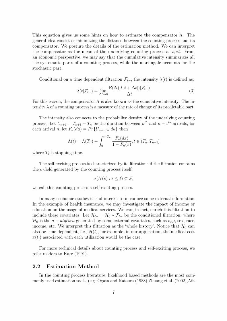
In many economic studies it is of interest to introduce some external information.In the example of health insurance, we may investigate the impact of income oreducation on the usage of medical services. We can, in fact, enrich this filtration toinclude these covariates. Let Ht− = H0 ∨ Ft− be the conditioned filtration, whereH0 is the σ − algebra generated by some external covariates, such as age, sex, race,income, etc. We interpret this filtration as the ‘whole history’. Notice that H0 canalso be time-dependent, i.e., H(t), for example, in our application, the medical costx(ti) associated with each utilization would be the case.

For more technical details about counting process and self-exciting process, werefer readers to Karr (1991).

2.2 Estimation Method

In the counting process literature, likelihood based methods are the most com-monly used estimation tools, (e.g.,Ogata and Katsura (1988),Zhuang et al. (2002),Aıt-

7

Sahalia et al. (2015),Bacry and Muzy (2014) and Mohler et al. (2012)). One require-ment of using them is the predictability of the cumulative intensity Λ with respectto the filtration σ(Ng(s) : s ≤ t). That is, conditional on the filtration, the values ofall the explanatory variables at time t should be known and observed just before t.However, as pointed out by Kopperschmidt and Stute (2013), in many complicatedeconomic situations, there is little reason to maintain such an assumption. Instead,the cumulative intensity should respect external shocks or impulses. In that case, themodel is most likely not dominated and the likelihood methods are difficult to apply.

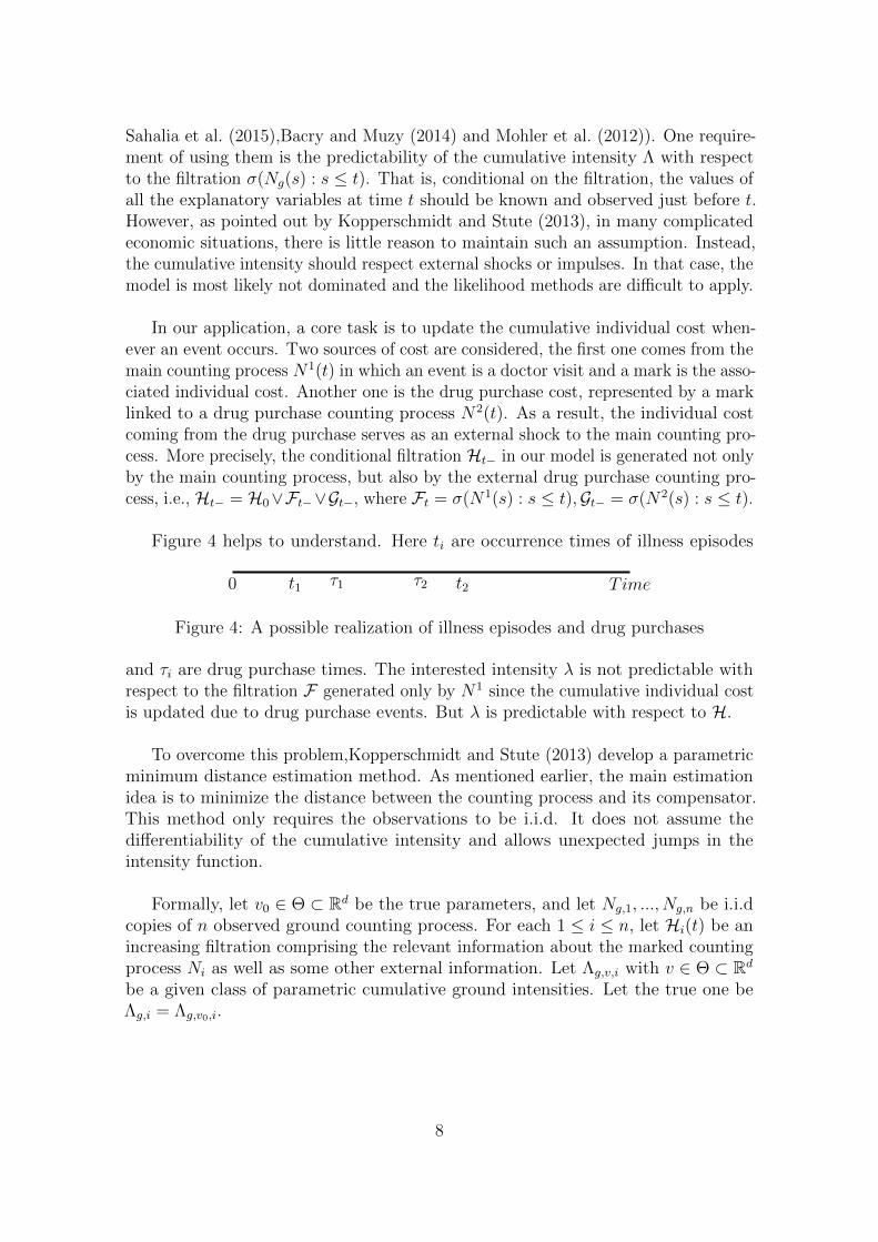
In our application, a core task is to update the cumulative individual cost when-ever an event occurs. Two sources of cost are considered, the first one comes from themain counting process N1(t) in which an event is a doctor visit and a mark is the asso-ciated individual cost. Another one is the drug purchase cost, represented by a marklinked to a drug purchase counting process N2(t). As a result, the individual costcoming from the drug purchase serves as an external shock to the main counting pro-cess. More precisely, the conditional filtration Ht− in our model is generated not onlyby the main counting process, but also by the external drug purchase counting pro-cess, i.e., Ht− = H0∨Ft−∨Gt−, where Ft = σ(N1(s) : s ≤ t),Gt− = σ(N2(s) : s ≤ t).

Figure 4 helps to understand. Here ti are occurrence times of illness episodes

0 t1 τ1 τ2 t2 Time

Figure 4: A possible realization of illness episodes and drug purchases

and τi are drug purchase times. The interested intensity λ is not predictable withrespect to the filtration F generated only by N1 since the cumulative individual costis updated due to drug purchase events. But λ is predictable with respect to H.

To overcome this problem,Kopperschmidt and Stute (2013) develop a parametricminimum distance estimation method. As mentioned earlier, the main estimationidea is to minimize the distance between the counting process and its compensator.This method only requires the observations to be i.i.d. It does not assume thedifferentiability of the cumulative intensity and allows unexpected jumps in theintensity function.

Formally, let v0 ∈ Θ ⊂ Rd be the true parameters, and let Ng,1, ..., Ng,n be i.i.dcopies of n observed ground counting process. For each 1 ≤ i ≤ n, let Hi(t) be anincreasing filtration comprising the relevant information about the marked countingprocess Ni as well as some other external information. Let Λg,v,i with v ∈ Θ ⊂ Rd

be a given class of parametric cumulative ground intensities. Let the true one beΛg,i = Λg,v0,i.

8

Let,

Nn =1

n

n∑i=1

Ni; Λv,n =1

n

n∑i=1

Λv,i (4)

We call the former averaged point process and the latter averaged cumulative intensity.Naturally the associated averaged innovation martingale is,

dMn = dNn − dΛv0,n (5)

The optimization object is:

||Nn − Λv,n||Nn(6)

Where

||f ||µ = [∫ T

0f 2dµ]1/2

T is a terminating time. This statistic 6 is an overall measurement of fitness of Λv,n

to Nn. The estimator vn is computed as,

vn = arg infv∈Θ||Nn − Λv,n||Nn

(7)

Kopperschmidt and Stute (2013) show this estimator is consistency and itsasymptotic behaviour is

√nΦ0(v0)(vn − v0)→ Nd(0, C(v0)) (8)

where

Φ0(v) =∂

∂v

∫E

(EΛv(t)− EΛv0(t))E∂

∂vΛv(t)

TEΛv0(dt) (9)

C(v0) is a d× d matrix with entries

Cij(v0) =

∫E

φi(x)φj(x)EΛv0(dx) (10)

and

φi(x) =

∫[x,t]

E∂

∂viΛv(t)EΛv0(dt) |v=v0 ,¯

t ≤ x ≤ t (11)

9

Remark Let Φn be the empirical analog of Φ0,

Φn(v) =∂

∂v

∫E

(Λv,n(t)− Λv0,n(t))∂

∂vΛv,n(t)T Λv0,n(dt) (12)

Since all Λg,v,n are sample means of i.i.d non-decreasing processes, a Glivenko-Cantelliargument yields, with probability one, uniform convergence of Λg,v,n → EΛg,v(t) ineach t on compact subsets of Θ, we have the expansion,

Φn(v) = Φ0(v) + op(1) (13)

Such expansion guarantees that in a finite sample situation, we can replace theunknown matrix Φ0(v0) by Φn(vn) and C(v0) by Cn(vn) without destroying thedistributional approximation through Nd(0, C(v0)), where Cn is the sample analogof C. In practice, one needs to plug and replace the true ones with estimators andreplace EΛv0(dt) with its empirical counterpart N(dt).

In the original Kopperschmidt and Stute (2013) paper, the authors do not providea numerical simulation study. Here we complete the task by generating a self-excitingprocess and examining the performance of the minimum distance estimator.

The data generating process we picked is the ETAS (epidemic type aftershocksequence) model. It was first introduced by Ogata and Katsura (1988) and eversince has been widely used in seismology (e.g. Zhuang et al. (2002)). It characterizesearthquake times and magnitudes and belongs to a marked Hawkes process family.The ETAS model has the probabilistic structure we desire: marks are part of theground intensity and can be separated into ground intensity and conditioned markdensity.

The intensity of a ETAS model, for its simplest form, could be:

λg(t|Ft−) = µ+∑i:ti<t

eαxi

(1 +

t− tic

)−1

(14)

where xi is the magnitude of an earthquake occurring at time ti, and the markdensity, for simplicity, is assumed to be i.i.d:

f(x|t,Ft−) = δe−δx (15)

We set the true parameters as µ = 0.007 , α = 1.98 , c = 0.008 and δ = log(10).The simulation method we used is called the thinning method, introduced by Ogata(1981), Lewis and Shedler (1979). Briefly, this method first calculates an upperbound for the intensity function in a small time interval, simulating a value for thetime to the next possible event using this upper bound, and then calculating theintensity at this simulated point. However these ‘events’ are known to be simulated

10

too frequently (Lewis and Shedler, 1979). To overcome this, the method will com-pare the ratio of the calculated rate with the upper bound to a uniform randomnumber to randomly determine whether the simulated time is treated as an eventor not (i.e. thinning). A full description of the algorithm is provided in the Appendix.

We generate N = 50, N = 100 and N = 200 individual counting processes for eachrepeat of the simulation and in total we have B = 1000 repeats. The time-intervalsare set to be [0, 3000], [0, 500] and [0, 100].

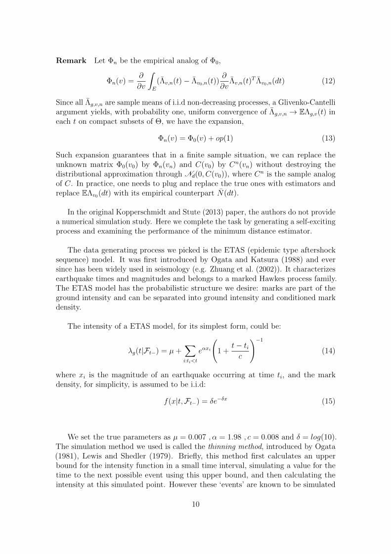
The estimation results are presented in Tables 1-3. As the number of observationsN increase, the estimators become more stable and their empirical coverage rate getscloser to the theoretical ones. It is also noticeable that the performance of estimatorsis insensitive to the number of events per person. (We increase the length of thetime horizon to increase such a number under the same true parameters.)

Table 1: Minimum Distance Estimator Results, with T = 3000N = 400 True MDE se CI95 CI90

µ 0.007 0.006957441 0.0006271522 94.9% 92. 5%α 1.98 1.978269 0.07331051 93.5% 90.8%c 0.008 0.008130796 0.001724244 93.9% 91.3%

Distance 1.48622 0.715594N = 200

µ 0.007 0.006960397 0.0008400477 93.6% 88.3%α 1.98 1.984108 0.1086315 93.2% 90.9%c 0.008 0.008042743 0.002413533 92.6% 90.3%

Distance 2.183783 1.226474N = 100

µ 0.007 0.00684719 0.0011465 93.4% 90.9%α 1.98 1.964071 0.1654297 92.1% 90.1%c 0.008 0.008570634 0.003605053 92.3% 90.5%

Distance 3.169824 2.388298N = 50

µ 0.007 0.006809876 0.001541488 89.1% 84.9%α 1.98 1.974604 0.2765146 87.9% 83.7%c 0.008 0.008979804 0.005475683 86.9% 83.1%

Distance 4.293006 3.474963Note: The distance is calculated using the semi-norm 6 with true parameters andthe minimum distance estimators, respectively.se is the mean of the standard errorof each simulation. CI95(CI90) is the percentage of the 95%(90%) confidenceinterval generated by se that covers the true parameter.

11

Table 2: Minimum Distance Estimator Results, with T = 500N = 400 True MDE se CI95 CI90

µ 0.007 0.006818704 0.001282338 95.3% 93%α 1.98 1.985548 0.2580961 96.3% 93.7%c 0.008 0.008327916 0.005313165 96% 92%

Distance 0.2336264 0.1619424N = 200

µ 0.007 0.007056179 0.001783448 92.5% 89.6%α 1.98 1.977045 0.4486648 91.9% 90.6%c 0.008 0.009058691 0.008174076 91.5% 89.9%

Distance 0.3579916 0.2119269N = 100

µ 0.007 0.00660844 0.002295691 90.1% 86.1%α 1.98 1.76104 0.85060127 86.6% 83%c 0.008 0.01662388 0.0174853 86.7% 83.7%

Distance 0.477976 0.4551476N = 50

µ 0.007 0.006672302 0.002964079 90.3% 88%α 1.98 1.761366 2.207844 91.4% 88.9%c 0.008 0.01808354 0.02508167 90.6% 87.8%

Distance 0.6452985 1.087129Note: The distance is calculated using the semi-norm 6 with true parameters andthe minimum distance estimators respectively. se is the mean of the standard errorof each simulation. CI95(CI90) is the percentage of the 95%(90%) confidenceinterval generated by se that covers the true parameter.

12

Table 3: Minimum Distance Estimator Results, with T = 100N = 400 True MDE se CI95 CI90

µ 0.007 0.0067466 0.002320197 95.2% 92.9%α 1.98 1.980313 1.687546 95.1% 94%c 0.008 0.01027362 0.01646008 95.4% 93.9%

Distance 0.0365799 0.0204637N = 200

µ 0.007 0.006614259 0.002845468 93.6% 90.6%α 1.98 1.91999 2.273823 94.5% 93.3%c 0.008 0.01357907 0.02549106 93.2% 92.1%

Distance 0.05125482 0.03664879N = 100

µ 0.007 0.01317505 0.005716749 81.5% 75.7%α 1.98 1.719879 2.227818 92.2% 89.6%c 0.008 0.02089188 0.03664059 89% 86.9%

Distance 0.6294044 0.1808156N = 50

µ 0.007 0.01273163 0.006974369 85.9% 82.9%α 1.98 1.87436 3.961052 95.6% 93.5%c 0.008 0.02130184 0.04548218 89.2% 87.2%

Distance 0.639077 0.1674467Note: The distance is calculated using the semi-norm 6 with true parameters andthe minimum distance estimators respectively. se is the mean of the standard errorof each simulation. CI95(CI90) is the percentage of the 95%(90%) confidenceinterval generated by se that covers the true parameter.

13

3 The Data

The data we used come from the well-known RAND Health Insurance Experiment(RAND HIE), one of the most important health insurance studies ever conducted. Itaddressed two key questions in health care financing:

1. How much more medical care will people use if it is provided free of charge?

2. What are the consequences for their health?

The HIE project was started in 1971 and was funded by the Department of Health,Education, and Welfare. The company randomly assigned 5809 people to insuranceplans that either had no cost-sharing, 25%, 50% or 95% coinsurance rates. Theout-of-pocket cap varied among different plans. The HIE was conducted from 1974to 1982 in six sites across the USA: Dayton, Ohio, Seattle, Washington, Fitchburg-Leominster and Franklin County, Massachusetts, and Charleston and GeorgetownCounty, South Carolina. These sites represent four census regions (Midwest, West,Northeast, and South), as well as urban and rural areas.

Early literatures that use this data usually avoid the problem of non-linear budgetconstraint by assuming that individuals only respond to one price system. Typicaleconometric tools involved are the linear regression (after aggregating the data), thecount data regression and the duration analysis. None of them is capable to fullymodel the stochastic structure of cumulative individual cost X(t).

Because the complicated structure of our self-exciting process, to ease the burdenof computation, we only use data from Seattle, which has the largest medical claimrecords available. We separate the data according to two different insurance plans:zero coinsurance rate plan (free plan, denoted as P0), in which the patient does notpay anything; and a cost-sharing plan (denoted as P95) in which a coinsurance rateof 95% applied and OPC is 150 USD per person or 450 USD per family2(i.e., beforeexceeding the OPC, individuals need to pay 95% of the medical care cost, once theOPC is reached, all the cost is paid by the insurance.). The OPC and coinsurancerate in this plan only applied to ambulatory services; inpatient services were free.Both plans covered a wide range of services. Medical expenses included servicesprovided by non-physicians such as chiropractors and optometrists, and prescriptiondrugs and supplies. There is no deductible in this insurance contract. The followingfigure summarizes the P95 contract design.

We also include the data of drug purchase records with information such as thepurchase dates and the values of non-covered charges. As discussed in the previoussection, we may treat the drug purchase as another counting process and as anexternal shock to our primary one (doctor-visiting counting process). In the originaldataset, one individual may have several claims in one day, and we combine all claims

2In 1973 dollars.

14

Total Expenditure

(Nom

inal

)In

div

idual

Cos

tX

(t)

OPC

A

tan−1(0.95)

Point A is the OPC . When the total expenditure is below A, the co-insurance (slope) r = 0.95 isapplied. Whenever the total expenditure is beyond A, there is no cost for individuals.

Figure 5: Contract design for P95

with an identical date into one and sum the non-covered charges.

The occurrence time stamp is defined as the annual duration between the be-ginning date of the insurance policy and the date this person visited a health careinstitution. For example, if the insurance begins on Jan-01-1977 and the date of adoctor visit is Oct-01-1977, the time stamp is then 0.748 (years). When preparingthe dataset, we delete all the records with missing duration information. (Hence weexclude the cases of censoring.)

When analyzing the cost-sharing plan, we restrict our dataset within the contractyear 1977-1978 since the cost-sharing policies are renewed annually. But such restric-tion is not needed for the free plan since there is no within-year cost sharing policy.For this plan, the time horizon ranges from 1975 to 1980. When the individual costinformation is missing, we replace it with zero. In the end, we have 243 individuals inthe free plan with 7638 claims over the years and 131 individuals in the cost-sharingplan and the total number of claims is 1103 within the 1977-1978 contract year.

We also include some demographic covariates: age, sex, education (in terms ofschooling years) and log-income. For simplicity, we fixed all ages at the enrolmenttime. Thus all covariates are time-independent. More covariates can be added, butwe are limited by computation capacity.

4 The Model

As discussed before, the focal point of the self-exciting counting process approachis to model the (cumulative) intensity function. We construct the intensities by

15

explicitly taking different randomness sources of cumulative individual cost X(t) andepisode dependence structure into consideration.

We further assume that 1) the initial event (or equivalently, the duration for thefirst doctor-visiting event under a new insurance contract) is given. Thus, we arenot interested in modeling the first event, and the counting processes exclude all thefirst events. 2) There is no unobserved heterogeneity.

The second assumption seems to be strong at first glance. However, we willprovide evidences to justify it in later section.

4.1 Free Insurance Plan

Our intensity λ(t) for each individual3 who belongs to the free insurance planconsists of two parts:λ(t) = λ1λ2(t). λ1 deals with the covariates effect, while λ2 isthe state-dependent (SD) term.

Like many count data regression and duration models, the covariates effect ispresented as an exponential function:

λ1(Z) = exp(γTZ) (16)

where Z is a vector of individual characteristics including age, sex, education andlog-income, etc.

The SD term is specified as:

λ2(t) =

N(t−)∑i=1

µ · exp(−µ(t− ti)), µ > 0 (17)

The ‘kernel’ µ · exp(·) characterizes the episode dependence structure. More specifi-cally, the propensity of a follow-up visit is governed by such a ‘kernel’: the intensity ishigh when the elapsed time is short and will gradually decrease as time goes by. Wewill argue such an assumption is reasonable: the individual is vulnerable when shejust receives the treatment and is more likely to be sick again, but she will graduallyrecover as time goes by and will be less likely to experience sickness. The summationover these ‘kernels’ means we take all the past episodes into consideration. But theweight for each episode is different. By construction, the effects of far away pastexperiences will deteriorate, but the latest ones have the most important influences.

The usual method to model such phenomena in a structural form model is toassume health events arrive periodically with a probability S

′, which is drawn from

F (S′|S) where S is the arrival probability from a previous period. Einav et al. (2015)

further simplify this assumption by letting S take one of two values, SL and SH

3Therefore, we ignore the individual subscript.

16

(with SL < SH), and that Pr(S′

= SJ |S = SJ) ≥ 0.5, J ∈ {L,H}, so there is weaklypositive serial correlation. This exceedingly simplified assumption is made mainlyfor computational reasons. The above Markov process is most likely inadequate tomodel the episode cluster structure. We believe our cluster set up is more realisticand is quite difficult, if not impossible, to build within the conventional econometricmodels.

To sum up, for the free insurance plan, P0, the intensity is expressed as:

λP0(t) = λ1(Z)λ2(t) (18)

4.2 Cost-Sharing Insurance Plan

As for the cost-sharing plan, λ1 does not change. The cost sharing policy hastwo hypothetical effects: 1) The late year effect, that is when the contract yearis near the end, individuals, especially those who have already exceeded the OPCmay use the medical service more frequently than before (cash-in effect) since thecost-sharing policy will be set to default next year and the shadow co-insurancerate would be expensive once again. 2) The shadow price effect discussed in theintroduction section. We update the cumulative individual cost whenever an eventoccurs. To account for the cost-sharing effects, we modify λ2 as follows:

λ∗2(t) = β1exp(β1t) +

N(t−)∑i=1

b exp(β2X(ti))µexp(−µ(t− ti)) (19)

Here X(t) is the cumulative individual cost at time t. It includes the non-coveredcharge from outpatient medical utilization as well as drug purchase:

X(t) =

N1(t−)∑i=1

xi +

N2(t−)∑i=1

yi (20)

where xi is the non-covered charge for ith doctor visiting, N1(t) is the associatedground counting process. yi is the non-covered charge for ith drug purchase and N2(t)is the drug purchase ground counting process. The construction of X(t) essentiallyfollows the definition of cumulative individual cost mentioned in the introductionsection. Recall the shadow price is defined as 1 − V (X(t)), where V (X(t)) is thebonus which depends on the cumulative individual cost. If V (X(t)) ∝ exp(β2X(t)),then the term b exp(β2X(t)) can be thought of as a measure of medical utilizationbonus. We would expect β2 > 0 to be significant if individuals do respond to shadowprice.

We use the term β1exp(β1t) to model the late year effect: we would observe β1

significantly greater than zero if such an effect is true.

To summarize, the ground intensity for the cost-sharing plan is:

λP95(t) = λ1(Z)λ∗2(t) (21)

17

There are several pieces to put together in order to estimate the parameters ofthe cost-sharing effects model. As Keeler and Rolph (1988), we assume that thereare no interactions between within-year cost sharing effects and the effects of otherexplanatory variables, so that all the effects of explanatory variables other thancost sharing on frequencies of episodes are summarized in λ1(Z) and all episodedependence structure is captured by λ2(t) (λ

′2(t)). We first estimate the free plan by

minimizing

||NP0 − λ1(Z)∫ T

0λ2(t)dt||NP0

thus, the individual heterogeneity and the episode dependence structure of theintensity are estimated by λ1(Z) and λ2(t). When estimating the cost-sharing plan,these two parts are then treated as fixed, which leaves us with only cost-sharingeffect parameters (i.e.,β1, β2 and b ) to be estimated (We exploit the fact that allindividuals are assigned to different plans randomly. By plugging the individualspecific estimators from the free plan into the cost-sharing plan, we can still haveconsistent estimators). Thus the minimization object is:

||NP95 − λ1(Z)∫ T

0

(β1exp(β1t) +

∑Ng(t−)i=1 b exp(β2X(ti))µexp(−µ(t− ti))

)dt||NP95

5 Main Results

The main results are presented in Table 4.

5.1 Interpreting the Covariates

The interpretation of coefficients is not as straightforward as in linear regression.However, we may fix a time period and treat the counting process as count data. Theinterpretation is then identical to that of a count data regression analysis. Formally,recall the Doob-Meyer decomposition, for a fixed time period [0, t], ∀t ∈ [

¯t, t], we

haveE(Λ(t|Z)) = E(N(t)|Z) = E(Yt|Z)

The count data Yt is the number of events occurring during this time period. Letscalar zj denote the jth covariate. Differentiating

∂E(Yt|Z)

∂zj= γjE(Λ(t|Z))

by the exponential structure of λ1(Z). That is, for example, if γj = 0.2, Λn(t|Z) = 2.5,then one-unit change in the jth covariate increases the expectation of Yt by 0.5 units.

With these in mind, we can interpret our results.

Age. The overall effect for age is as follows: at first, the intensity will decrease asage increases, after one passes the age of 41.5, the intensity and age are positivelycorrelated. It is well-known that the youngsters are more risky compared to their

18

Table 4: Basic Results

Estimator Description

µ 25.264612∗∗∗ coefficient of the episode dependent structure(4.230528)

age -0.230274∗∗∗

(0.084052)

age2 0.277269∗∗∗ (age)2/100(0.115787)

male -0.554904(0.447628)

edu -0.190387(0.204672)

edu2 0.184098 (edu)2/100(0.862468)

log income 0.685771∗∗∗

(0.141580)

b 0.65898635∗∗∗

(0.0580308)

β1 0.1068388 coefficient of late year effect(0.27547018)

β2 0.00383393∗∗∗ coefficient of non-covered charge(0.00061892885)

Distance 1.00747 Free PlanDistance 1.10226 Cost-Sharing Plan

Note: standard errors in brackets, ∗p<0.1; ∗∗p<0.05; ∗∗∗p<0.01

19

mid-age counterparts. While as individuals begin to age, they become physicallyweaker and more prone to sickness.

Sex. Females seem to be more likely to go the doctor, but the result is notsignificant.

Education. The multi-parameter Wald Test Statistics for edu = edu2 = 0is 13.33125, indicating the education is a significant factor to the doctor-visitingbehaviors. The result suggests a negative relation between education and theoutpatient medical utilization. One explanation could be that individuals with ahigher level of education are positioned in more important jobs and their absencefrom work may damage not only their output but also that of their peers’, thusthe potential cost of going to hospital is much higher which leads to a negativecorrelation.

Income. Income is positively related to the use of medical services, which is notsurprising. A higher income gives individuals the ability to cover the opportunitycost related to absence from work (to visit a doctor).

The shadow price effect is captured by b exp(β2R(t)). The most important pa-rameter here is β2. If β2 is close enough to zero, we may observe a flat, almost linearcurve, which indicates that individuals only respond to one price system (the spotprice system). However, if β2 is positively away from zero, we can safely claim thatindividuals do understand the design of the insurance policy and take advantage ofthe shadow price. Our result provides strong evidence for the shadow price effectand we are confident to reject the null hypothesis: β2 = 0.

There is weak evidence supporting the existence of the late year effect.

5.2 Little Unobserved Heterogeneity Effect Evidence

In a variety of contexts, it is often noticed that individuals who have experiencedan event in the past are more likely to experience the event again in the futurethan are individuals who have not experienced the event (Heckman, 1981). Oneexplanation, best known as the unobserved heterogeneity, is that in addition tothe observed variables, there are other relevant variables that are unobserved butcorrelated with the observed ones.

Another explanation of heterogeneity is related to state dependence (SD). Thisconcept says that past experience has a genuine effect on future events in a sensethat an otherwise identical individual who did not experience the event would behavedifferently in the future. The definition of the self-exciting process naturally includesthe idea of state dependence.

Compare with the usual unobserved heterogeneity settings, the state dependencediffers in several ways. First, the SD term is time dependent, which means that it canbe updated, while the typical UH term is time persistent. Second the choice of theSD term is flexible and can be consistent with economic theory. For example, we may

20

capture the seasonality effect by setting the term as K(ti, t) = αsin(β(t− ti) +γ) + δ,or in our application, we may study the cluster phenomenon of medical care utiliza-tion by letting K(ti, t) = µexp(−µ(t− ti)), µ > 0.

Before presenting evidences on little unobserved heterogeneity, we would like todemonstrate that a self-exciting process can generate enough heterogeneity withoutintroducing a latent variable to represent the unobserved heterogeneity.

The data generating process (DGP) is the same as in the simulation studiesbefore. Figure 6 presents three quite different individual’s event histories simulatedby this DGP using the identical parameter settings as stated before.

Individual 1 has the most frequent events experience, the total number of eventsis 92. Individual 2 is somewhat moderate, with 37 events. Individual 3 has the leastfrequent events with only 2 during the time interval [0, 100].

We now present some evidences on the little unobserved heterogeneity effect.

5.2.1 Evidence One: Modeling the Initial Duration Using Heckman andSinger’s NPMLE

The subject under study here is the initial duration to visit a doctor under thefree plan.

In the main model, we assume that the initial duration is given. Here we take theadvantage that the initial event under a new free insurance plan can be reasonablyassumed to be free from any state dependent effect such that if there exists anyunexplained heterogeneity, it should come from the unobserved term.

We specify the hazard rate and its cumulative hazard function for the initialduration as:

hi(νi, Xi) = exp(X ′iβ + νi)

Hi(t) = hi(νi, Xi)t

where νi is the unobserved heterogeneity and Xi is a vector of observed covariates.The likelihood contribution of each individual is

Li = exp(−Hi(t))hi(νi, Xi)

Assume ν ∼ G is independent from Xi, one may use Heckman and Singer (1984)’snon-parametric maximum likelihood estimator (NPMLE) to avoid unjustified as-sumptions about the distribution G. Instead, one may approximate G in terms of a

21

(a) Individual 1, Event Time (b) Individual 2, Event Time

(c) Individual 3, Event Time

(d) Individual 1, log of intenstiy (e) Individual 2, log of intenstiy

(f) Individual 3, log of intenstiy

Figure 6: Three individual’s events histories

22

discrete distribution.

LetQ be the (prior unknown) number of support points in this discrete distributionand let νl, pl, l = 1, 2, · · · , Q be the associated location scalars and probabilities. Thelikelihood contribution is:

E[Li(νi)] =

Q∑l=1

plLi(νl),

Q∑l=1

pl = 1

where Li(νl) = exp(−Hi(t|νl, Xi))hi(t|νl, Xi).

The likelihood function is

L =N∏i=1

E[Li(ν)] =N∏i=1

Q∑l=1

plLi(νl),

Q∑l=1

pl = 1

The estimation procedure consists of maximizing the likelihood function withrespect to β as well as the heterogeneity parameters νl and their probabilities plfor different values of Q. Starting with Q = 2, and then expanding the model withnew support points until there is no gain in likelihood function value. Heckman andSinger (1984) has proven that such an estimator is consistent, but its asymptoticdistribution has not been discussed yet.

If there is little unobserved heterogeneity, one would expects that when Q = 2,one of the mass point probability, say, p1 ≈ 1 and the other p2 ≈ 0, in addition, theheterogeneity parameters should be similar in value ν1 ≈ ν2.

Table 5 shows exactly this situation.

5.2.2 Evidence Two: Group Heterogeneity on the Initial Duration

Instead of assuming individual heterogeneity, one might assume the group het-erogeneity and reveal the group affiliation through an external model. Such a typicalmodel is the finite mixture model.

Assume individuals belong to k different groups and the initial duration yi aregoverned by a finite mixture reverse Gumbel:

p(y|Θ) = w1f1(y|Θ1) + w2f2(y|Θ2) + · · ·+ wkfk(y|Θk)

where Θ = (Θ1,Θ2, · · · ,Θk,w)′denotes the vector of all parameters, w = (w1, w2, · · · , wk)

′

is a vector of weight whose elements are restricted to be positive and sum to unity.fk(·|Θk) is a reverse Gumbel density with the vector of parameters Θk.

Additionally, we may equivalently model the finite mixture model in a hierarchicalmanner using a latent variable li, which represents the allocation of each observation

23

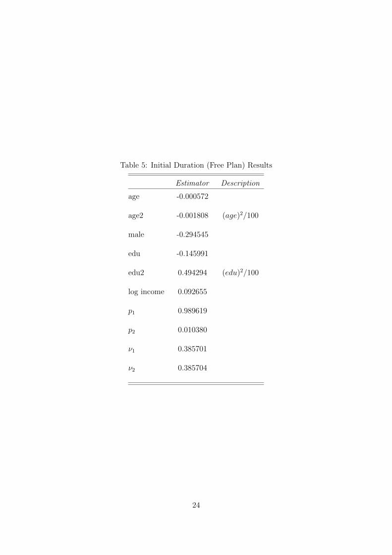
Table 5: Initial Duration (Free Plan) Results

Estimator Description

age -0.000572

age2 -0.001808 (age)2/100

male -0.294545

edu -0.145991

edu2 0.494294 (edu)2/100

log income 0.092655

p1 0.989619

p2 0.010380

ν1 0.385701

ν2 0.385704

24

yi to one of the components:

p(yi|Θk, li = k) = fk(yi|Θk)

p(li = k) = wk

One may have the group affiliation posterior by the Bayesian rule:

p(li = k|yi,Θk) =p(yi|li = k,Θk) ∗ p(li = k)

p(yi|Θk)

=p(yi|li = k,Θk) ∗ wk∑Kk=1 p(yi|li = k,Θk) ∗ wk

we may then assign the group affiliation according to the posteriors.

For simplicity, we assume group number k = 2.

The typical estimation method for a finite mixture model is the EM algorithm.Once we ‘reveal’ each individual’s group affiliation, we might include this new covari-ate into our main model. If there is little unobserved heterogeneity effect, we shouldexpect the coefficient for this new covariate to be insignificant from zero.

Table 6 reports the results and further confirm that there is indeed little un-observed heterogeneity effect. The multi-parameter Wald test statistic for age =age2 = 0 is 567.885, the statistic for edu = edu2 = 0 os 10.719, indicating both ageand education is significant. However, the group effect is not significant.

5.2.3 Evidence Three: Group Heterogeneity on counts

Similar to what we did before, here, instead of modeling the initial duration, wemodel the number of doctor-visiting for five years under a free plan.

Again, we assume the number of group k = 2, and the interested parameterwould be the coefficient of the group affiliation.

Table 7 reports the results, which further confirm that there is little unobservedheterogeneity.

One possible explanation for this little heterogeneity effect could be this: thesubject under this study is the outpatient doctor-visiting, which is mostly caused byminor episodes and injuries. If an individual has not experienced any illness in arelatively long period, then the unobserved heterogeneity might contribute to thenext illness, but the effect from the state dependent structure is the dominating causefor the future doctor-visiting. That is this initial illness might cause next episodesand this structure outweighs the individual’s unobserved heterogeneity.

To sum up, conditional on a state dependent structure, the unobserved hetero-geneity plays little roles (as best demonstrated in the Evidence Two) in individual’sdoctor-visiting behaviors, at least for outpatient case.

25

Table 6: Group Heterogeneity on Initial Duration (Free Plan) Results

Estimator Description

µ 29.035433∗∗∗ coefficient of the episode dependent structure(4.935501)

age -0.124143(0.10111)

age2 0.146278 (age)2/100(0.13168)

male -0.442570(0.44991)

edu -0.134448(0.18627)

edu2 0.254624 (edu)2/100(0.69313)

log income 0.396356∗∗∗

(0.17695)

Group 0.561757 Group affiliation(0.613766)

Distance 0.631360 Free Plan

Note: standard errors in brackets, ∗p<0.1; ∗∗p<0.05; ∗∗∗p<0.01

26

Table 7: Group Heterogeneity on counts (Free Plan) Results

Estimator Description

µ 28.270280∗∗∗ coefficient of the episode dependent structure(8.267194)

age -0.149708∗∗∗

(0.030242)

age2 0.174288∗∗∗ (age)2/100(0.045306)

male -0.599141(0.588516)

edu -0.417321∗∗∗

(0.085243)

edu2 1.195932∗∗∗ (edu)2/100(0.360884)

log income 0.64824∗∗∗

(0.042359)

Group 0.301163 Group affiliation(0.377391)

Distance 0.864397 Free Plan

Note: standard errors in brackets, ∗p<0.1; ∗∗p<0.05; ∗∗∗p<0.01

27

5.3 Cluster Analysis

The episodes tend to be clustered or grouped together (i.e., we are rejecting theassumption that episodes are independent). One reason is because of the natureof chronic diseases: regular or frequent treatments are needed to ease or eliminatethe pain. Another explanation is because one disease may trigger the occurrence ofanother one in the short term.

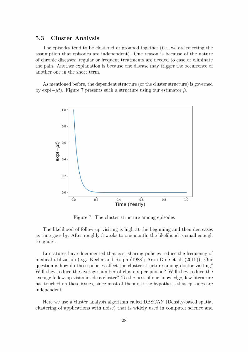
As mentioned before, the dependent structure (or the cluster structure) is governedby exp(−µt). Figure 7 presents such a structure using our estimator µ.

Figure 7: The cluster structure among episodes

The likelihood of follow-up visiting is high at the beginning and then decreasesas time goes by. After roughly 3 weeks to one month, the likelihood is small enoughto ignore.

Literatures have documented that cost-sharing policies reduce the frequency ofmedical utilization (e.g. Keeler and Rolph (1988); Aron-Dine et al. (2015)). Ourquestion is how do these policies affect the cluster structure among doctor visiting?Will they reduce the average number of clusters per person? Will they reduce theaverage follow-up visits inside a cluster? To the best of our knowledge, few literaturehas touched on these issues, since most of them use the hypothesis that episodes areindependent.

Here we use a cluster analysis algorithm called DBSCAN (Density-based spatialclustering of applications with noise) that is widely used in computer science and

28

statistical learning.

For this algorithm, there are two inputs: Eps, the radius of one density region,and minPts, the minimum number of points required to form a dense region. For thepurpose of DBSCAN clustering, all points are classified as core points, border pointsand noise points. Core and border points form a cluster via different definitionsof ‘reachable’. Noise points are the points that do not belong to any cluster. Weprovide details of this algorithm and the definition of a cluster in the Appendix.

The ability of this algorithm to identify ‘noise’ points is particularly appealing tous. This is because some acute episodes are small in scale and only need one doctorvisit to fully recover. They are not linked to the rest of episodes.

Based on the estimation of the SD term, we set Eps = 21 days and as a rule ofthumb minPts = 24. For the purpose of comparison, we restrict the time horizonin both plans to 1977-1978 insurance year. For each individual (both free plan andcost-sharing plan), we run the DBSCAN algorithm, document the number of clusters,the average number of instances per cluster and the number of noise points. Foreach insurance plan, we then compute the average number of clusters per person,the average number of instances per cluster per person and the average noise pointsper person. Table 8 summarizes the results.

Table 8: Cluster Analysisavg cluster number avg cluster members avg noise points

free plan 1.2287 4.55187 1.62332Cost-sharing plan 0.862595 3.3625 1.47328

The effects of cost-sharing policies on cluster structure are threefold. First, theyreduce the average number of clusters per person. That means for the initial episode,the cost-sharing policies suppress the first doctor visiting behaviors. Second, withineach cluster, they reduce the number of follow-up visits. Third, cost-sharing policiesreduce the average number of noise points per person, i.e., they discourage individualsto use medical services when they have small episodes like minor injuries.

6 Conclusion

In this paper, we provide a methodology to construct a behavioral model ofmedical care utilization. At the core of this method is the self-exciting countingprocess. It allows researchers to take historical information into the model. Aminimum distance estimation is employed. By doing so, one may introduce externalshocks to the self-exciting process. This enables researchers to use more realisticmodel settings. We use such a methodology to build a decision making processmodel of medical care utilization and find that individuals are responsive to shadow

4The rule of thumb is minPts = dimension +1

29

price and take into account the dynamic incentives. Furthermore, using differentexternal models (Duration analysis on initial duration, finite mixture models), wefind that once taking the state-dependent structure into the model, the unobservedheterogeneity plays an insignificant role. Lastly, using a matured statistical learningalgorithm, we analyze the cluster structure of doctor visiting behaviors. We findcost-sharing policies do affect the clusters in numerous ways.

30

References

Yacine Aıt-Sahalia, Julio Cacho-Diaz, and Roger JA Laeven. Modeling financialcontagion using mutually exciting jump processes. Journal of Financial Economics,117(3):585–606, 2015.

Aviva Aron-Dine, Liran Einav, and Amy Finkelstein. The rand health insuranceexperiment, three decades later. Technical report, National Bureau of EconomicResearch, 2012.

Aviva Aron-Dine, Liran Einav, Amy Finkelstein, and Mark Cullen. Moral hazardin health insurance: do dynamic incentives matter? Review of Economics andStatistics, 97(4):725–741, 2015.

Emmanuel Bacry and Jean-Francois Muzy. Hawkes model for price and tradeshigh-frequency dynamics. Quantitative Finance, 14(7):1147–1166, 2014.

Zarek C Brot-Goldberg, Amitabh Chandra, Benjamin R Handel, and Jonathan TKolstad. What does a deductible do? the impact of cost-sharing on health careprices, quantities, and spending dynamics. The Quarterly Journal of Economics,132(3):1261–1318, 2017.

Liran Einav, Amy Finkelstein, and Paul Schrimpf. The response of drug expenditureto nonlinear contract design: Evidence from medicare part d. The quarterly journalof economics, 130(2):841–899, 2015.

Martin Ester, Hans-Peter Kriegel, Jorg Sander, Xiaowei Xu, et al. A density-basedalgorithm for discovering clusters in large spatial databases with noise. In Kdd,volume 96, pages 226–231, 1996.

Benjamin R Handel, Jonathan T Kolstad, and Johannes Spinnewijn. Informationfrictions and adverse selection: Policy interventions in health insurance markets.Technical report, National Bureau of Economic Research, 2015.

James Heckman and Burton Singer. A method for minimizing the impact of dis-tributional assumptions in econometric models for duration data. Econometrica:Journal of the Econometric Society, pages 271–320, 1984.

James J Heckman. Heterogeneity and state dependence. In Studies in labor markets,pages 91–140. University of Chicago Press, 1981.

Alan Karr. Point processes and their statistical inference, volume 7. CRC press,1991.

Emmett B Keeler and John E Rolph. The demand for episodes of treatment in thehealth insurance experiment. Journal of Health Economics, 7(4):337–367, 1988.

Emmett B Keeler, Joseph P Newhouse, and Charles E Phelps. Deductibles and thedemand for medical care services: The theory of a consumer facing a variable priceschedule under uncertainty. Econometrica, pages 641–655, 1977.

31

Kai Kopperschmidt and Winfried Stute. The statistical analysis of self-exciting pointprocesses. Stast. Sinica, 23:1273–1298, 2013.

Peter A Lewis and Gerald S Shedler. Simulation of nonhomogeneous poisson processesby thinning. Naval Research Logistics Quarterly, 26(3):403–413, 1979.

George O Mohler, Martin B Short, P Jeffrey Brantingham, Frederic Paik Schoenberg,and George E Tita. Self-exciting point process modeling of crime. Journal of theAmerican Statistical Association, 2012.

Yosihiko Ogata. On lewis’ simulation method for point processes. InformationTheory, IEEE Transactions on, 27(1):23–31, 1981.

Yosihiko Ogata and Koichi Katsura. Likelihood analysis of spatial inhomogeneity formarked point patterns. Annals of the Institute of Statistical Mathematics, 40(1):29–39, 1988.

Jiancang Zhuang, Yosihiko Ogata, and David Vere-Jones. Stochastic declustering ofspace-time earthquake occurrences. Journal of the American Statistical Association,97(458):369–380, 2002.

32

A The Thinning Method for Simulation

The detailed thinning method steps can be summarised as:

1. Let τ be the start point of a small simulation interval

2. Take a small interval (τ, τ + δ)

3. Calculate the maximum of λg(t|Ft−) in the interval as

λmax = maxt∈(τ,τ+δ)

λg(t|Ft−)

4. Simulate an exponential random number ξ with rate λmax

5. if

λg(τ+ξ|Ft−)

λmax< 1

go to step 6.

Else no events occurred in interval (τ, τ + δ), and set the start point atτ ← τ + δ and return to step 2

6. Simulate a uniform random number U on the interval (0, 1)

7. If

U ≤ λg(τ+ξ|Ft−)

λmax

then a new ‘event’ occurs at time ti = τ + ξ. Simulate the associated marksfor this new event.

8. Increase τ ← τ + ξ for the next event simulation

9. Return to step 2

B DBSCAN Cluster Analysis

The DBSCAN algorithm classified all points into three: core points, borderpoints and noise points. We start by defining these points. For a set of pointsX = {x1, x2, · · · , xN}.

Definition ε neighbourhood of a point x, denoted by Nε(x) is defined by Nε(x) ={y ∈ X : d(y, x) ≤ ε}. Where d() is a metric.

33

Definition Density is defined as ρ(x) = |Nε(x)|, the number of points in a εneighbourhood.

Definition Core point: let x ∈ X, if ρ(x) ≥ minPts, then we call x a core point.The set of all core points is denoted as Xc, let Xnc = X \Xc be the set of all non-corepoints.

Definition Border point: if x ∈ Xnc and ∃y ∈ X such that y ∈ Nε(x) ∩Xc, thenx is called a border point. Let Xbd be the set of all border points.

Definition Noise point: let Xnoise = X \ (Xc ∪Xbd), if x ∈ Xnoise, then we call xis a noise point.

To define what is a cluster under the DBSCAN setting, we need a few more definitionsabout ‘reachable’.

Definition Directly density-reachable: if x ∈ Xc and y ∈ Nε(x), we may say y isdirectly reachable from x.

Definition Density-reachable: let x1, x2, · · · , xm ∈ X,m ≥ 2. If xi+1 is directlydensity-reachable from xi, i = 1, 2, · · · ,m− 1. We call xm is density-reachable fromx1.

Definition Density-connected: a point x is density connected to a point y if thereexists another point z ∈ X such that both y and x are density-reachable from z.

Definition Cluster: a non-empty subset C of X is called cluster if it satisfies:

• (Maximality) ∀x, y: if x ∈ C and y is density-reachable from x, then y ∈ C.

• (Connectivity) ∀x, y ∈ C: x is density-reachable to y.

For a detailed algorithm description, we refer to the original Ester et al.(1996)Esteret al. (1996) paper.

34