THE COST OF FERTILITY IN CHINA:

DO CHINESE WOMEN POSTPONE THEIR FERTILITY DECISIONS BECAUSE

EDUCATION INCREASES THEIR RELATED OPPORTUNITY COST?

A Thesis

submitted to the Faculty of the

Graduate School of Arts and Sciences

of Georgetown University

in partial fulfillment of the requirements for the

degree of

Master of Public Policy

By

Yuchen Xiang, B.S.

Washington, DC

April 12, 2019

ii

Copyright 2019 by Yuchen Xiang

All Rights Reserved

iii

THE COST OF FERTILITY IN CHINA:

DO CHINESE WOMEN POSTPONE THEIR FERTILITY DECISIONS BECAUSE

EDUCATION INCREASES THEIR RELATED OPPORTUNITY COST?

Yuchen Xiang, B.S.

Thesis Advisor: Andreas Kern, Ph.D.

ABSTRACT

This research focuses on how education affects Chinese women’s fertility decisions. I

hypothesize that enhanced access to education has led to a postponement of pregnancies

among Chinese women and a decrease in the number of children they have. To test this

hypothesis, I use data from the China Nutrition and Health Survey on 8319 women who

have ever given birth in a set of standard OLS regression and Negative Binomial

Regression models. My findings indicate women with higher levels of education give birth

to their first child later in life. To verify this result, I perform a battery of robustness checks.

In particular, using an instrumental variables approach relying on information on a

woman’s siblings, I find that both education and individual annual income are significantly

correlated with fertility decisions. Against this background, I argue that, Chinese decision

makers need to find policy responses that account for the effects of education in order to

boost births and counter existing adverse population dynamics.

iv

Acknowledgements

The research and writing of this thesis is

dedicated to all women in the world of gender inequality.

Thanks to Professor Andreas Kern for Dedicated and Encouraging Instruction Regard to

Quantitative Research Analysis in the Field of Public Policy

Thanks to Professor Jeffery Mayer for Educational Editorial Advice

Thanks to Eric Gardner for the Strategies in Data Management

Many thanks,

Yuchen Xiang

v

Table of Contents

1. INTRODUCTION ...........................................................................................................1

2. LITERATURE REVIEW ................................................................................................3

2.1 Historical Context ......................................................................................................3

2.2 Fertility after 2000 ....................................................................................................5

3. HYPOTHESIS AND CONCEPTUAL FRAMEWORK ................................................8

3.1 Hypothesis..................................................................................................................8

3.2 Regression Models ...................................................................................................10

4. DATA DESCRIPTION ................................................................................................12

4.1 Data Source ..............................................................................................................12

4.2 Descriptive Statistics ................................................................................................13

4.3 Preliminary Findings ................................................................................................15

4.4 Empirical Results .....................................................................................................18

5. POLICY IMPLICATIONS ...........................................................................................27

6. CONCLUSION .............................................................................................................30

APPENDIX .......................................................................................................................31

REFERENCES .................................................................................................................39

vi

List of Figures

Figure 1. Density Distribution of the Age When a Woman Had First Birth ................16

Figure 2. Average Age of First-Time Mothers by Different Education Levels ............17

Figure 3. Boxplot Showing Distribution of Chinese Women’s Education Level .........18

List of Tables

Table 1. Specific Controls Included in OLS Regressions Using Age at First Birth .....11

Table 2. Descriptive Statistics on Chinese Mothers from 1995 to 2015 .......................15

Table 3. OLS Regression Using Age as Dependent Variable ......................................20

Table 4. Incident Rate Ratio Using Age as Dependent Variable ..................................21

Table 5. NBR Margins Using Age at First Birth as Dependent Variable .....................21

Table 6. OLS Regression Using Number of Children as Dependent Variable .............23

Table 7. Incident Rate Ratio Using Number of Children as Dependent Variable .........24

Table 8. NBR Margins Using Number of Children as Dependent Variable ................24

Table 9. Comparisons between OLS Regressions and OLS with Instrumental

Variable ...........................................................................................................26

1

1. Introduction

Until 2015, China’s One-Child Policy (OCP) limited Chinese families to have one child.

In 2015, however, in order to boost the country’s fertility rate, the government replaced

the OCP with a Second-Child Policy (SCP). Nonetheless, evidence shows that despite the

SCP, the country’s fertility rate has continued to fall, especially for highly-educated and

career-oriented Chinese women. From 2016 to 2018, according to the National Bureau of

Statistics, China’s birth rate dropped from 12.95 per 1,000 people to 10.94, which is the

lowest official birth rate since 1961 (Leng 2019).

This paper tries to explain why more educated women postpone having their first child

and why they are reluctant to have more than one child. In particular, it asks: what is the

role of higher education in this phenomenon? Are highly-educated women delaying the

decision to have children only because they want to build a successful career, or are there

other economic reasons, such as income levels and job constraints. Moreover, if

underprivileged families are contributing the most to the new-born population every year,

is it possible that in the near future, China will face a low human capital problem (a

retarded national education level)? Under this anticipated circumstance, what possible

policy alternatives can China design and implement to improve the overall working and

childbearing environment for households and to continue to produce high-quality human

capital?

To answer these questions, I use household- and individual-level data from the China

Health and Nutrition Survey. The survey has been conducted periodically from 1991 to

2015, and is a representative sample of Chinese households and individuals. The survey

variables I am especially interested in are mother’s date of birth, child’s date of birth,

child’s gender, and mother’s mean age at first birth, education level, and income level. I

2

am also interested in examining my questions by region, including urban and rural areas.

My data set also includes information about each respondent’s income level, employment

information, and education level, which allows me to test other factors that can impact

women’s decisions to have children. The raw sample size, before a thorough data

cleaning, is more than 50,000.

The dataset is quite precise in many aspects, including education level, mother’s

occupation, and mother’s income levels, and is sufficiently complete for operating

regression models and for exploring the questions motivating my research. From a policy

perspective, my findings indicate that Chinese women who live in urban and who have

obtained higher levels of education tend to have fewer children and have them later.

Conversely, women who live in rural area and have not received much education are

more likely to have more children and at an earlier age. In this case, education is a strong

indicator of Chinese women’s fertility behaviors.

3

2. Literature Review

2.1 Historical Context

On October 1st 1949, the supreme Chinese leader Mao Zedong officially announced the

creation of People’s Republic China, marking the end of the civil war between the

Chinese Communist Party and the Nationalist Party. At that time, China was trapped in

extreme poverty, because both the Second Sino-Japanese War and the Civil War had

imposed huge costs in blood and treasure. In response, Mao advertised the principle

“More people, more power” to boost China’s fertility rate during that period so that there

could be more human capital devoted to agriculture. During the 1950s and 1960s,

Chinese officials began to recognize the troubles introduced by overpopulation, but the

Great Leap Forward and Cultural Revolution in 1967 stopped any efforts to prevent it.

Mao died in 1976, the Cultural Revolution ended, and Deng Xiaoping rose to power as

paramount leader. Under Deng’s leadership, government officials, recognizing the

decrease in China’s living standards induced by overpopulation, stressed the importance

of birth control, and in 1979 formally introduced the One-Child Policy as an essential

method to alleviate poverty and improve living standards (J. Zhang 2017).

The One-Child Policy limited Chinese families to a single child. However, the policy was

implemented most stringently in urban areas. In rural areas, families were allowed to

have a second child if their first one was a girl (J. Zhang 2017). Moreover, the hukou

system, through which the government was able to monitor the fertility behaviors of

families (Xuebo Wang 2018), was more fully established in urban areas. If an urban

4

couple had a second child, they had to pay a penalty and could lose their jobs and social

benefits. Thus, even though the One-Child Policy reduced family size nationally, the

decrease of family size was relatively smaller in rural areas than in urban areas.

In fact, the effects of the OCP were multi-dimensional. First, it reduced the average

human capital level, because OCP was a two-tier policy. Problems arose not only because

rural families were allowed to have a second child, but also because the hukou system

was not well established in those areas, which made it extremely hard to keep track of

reproduction behaviors of rural families. Moreover, more than 53% of urban youth

attained education beyond secondary level; whereas only 9% of rural youth attained

education beyond the secondary level (Xuebo Wang 2018). Thus, the OCP eventually led

to a decrease in the country’s average education level.

Second, the OCP widened the education gap between rural and urban families. People

living in urban areas had access to better education resources and better employment

opportunities, so they were more likely to invest in their children. However, rural families

with more children did not enjoy such conditions, so their human capital investments

were lower (Xuebo Wang 2018). As a result, the average education level was much

higher for urban children than for rural children.

Third, the OCP resulted in a more rapidly aging population. The policy was implemented

in 1979 and lasted for 36 years, a period in which the life expectancy of Chinese people

increased from 67 to 75 years, and the fertility rate decreased from 2.8 to 1.6. As a result,

5

the share of China’s population 65 years old or older increased from 4% in 1960 to 11%

from in 2017.

Fourth, because it allowed rural families to have a second child if their first child was a

girl, the OCP increased the imbalance in China’s sex ratio. The rural exemption reflected

Chinese families’ preference for boys and the country’s heavy dependence on agriculture.

Rural families prefer boys because boys can contribute more to agricultural work and

thus increase family income (J. Zhang 2017). Currently, in China, about 118 boys are

born for every 100 girls.

Nonetheless, the OCP was effective in reducing China’s fertility rate. Evidence suggests

that about 18% of the decrease in fertility by the 1990s was due to the OCP. However, by

2000, other economic factors had become more important in determining Chinese

women’s fertility behaviors. Thus, it was predicted that the Second-Child Policy, initiated

in 2015, would have little effect on fertility rates (Garcia 2017). Arguably, therefore, the

Chinese government, in implementing the SCP to mitigate the problem of an aging

population, has not made the most effective policy decision.

2.2 Fertility after 2000

Due to the two-tier characteristic of the One-Child Policy, birth restrictions were

particularly binding on urban couples, who are also the major target the Second-Child

Policy. However, ever since the more relaxed birth restriction was implemented in 2015,

the country’s overall fertility rate has remained quite steady at approximately 1.6. Prior

6

studies have identified many factors other than birth restriction that can have significant

influence on women’s fertility, especially in the case of urban women. Women’s labor

market participation, socio-economic status, and cost of urban living have all been

significant in determining fertility in China, and education has played an important role in

improving women’s chances of getting jobs and raising their socio-economic status. This

section of my thesis explains these factors in more detail.

a. Labor Market Participation of Chinese Women

According to the Economic Theory of the Household, fertility and employment are

reciprocally related choices, and total amount of time is a constraining factor (Hai Fang

2012). This means that as a family has more children, the amount of time allocated to

work will be less. In Fang et al.’s (2002) analysis, the results show that off-farm

employment decreases women’s prefered number of children by 0.35, and their actual

number of children by 0.5. In the same study, the author found education to be a

significant factor that increases women’s participation in the labor market. In addition, as

a woman’s education level increases, her opportunity cost of having children also

increases.

However, as women’s participation in labor market increases, their corresponding social

welfare does not improve. Current maternity leave policy in China is not very friendly to

young women, allowing only 98 paid leave days, including working days, weekends, and

national holidays. Moreover, no laws ban discriminatory behaviors against females in the

workplace. A survey conducted by the All China Federation of Women shows that over

7

87% of female graduates have experienced explicit employment discrimination, such as

being asked whether they are single/married, being asked for a fertility plan, or facing

preference for men only (China Labor Bulletin 2018). Thus, in order to build a career and

be economically independent, women who attain higher education prefer fewer children

and have to postpone fertility decisions.

b. Socio-Economic Status of Chinese Women

Women’s improved status has contributed to China’s post-2000 fertility reduction. A

study of Chinese fertility decline and women’s status improvement shows that a wife

who is less economically dependent on her husband has more autonomy in making

decisions on child bearing, and may be more satisfied with her status (Xiaogang Wu

2014). To be more specific, if the wife’s total household income share is 50 percent or

greater, she will have more negotiating power in the marriage (Yue Qian 2018). Such a

finding provides a solid framework for my thesis because I assume that women who

attain more education are more likely to enter the labor market, thus making more

income. In this case, education is the source of the improvement in women’s socio-

economic status.

c. Cost of Living in Urban Areas

Another factor affecting women’s childbearing choices is the rising cost of living,

especially for young couples who live in metropolitan areas like Beijing and Shanghai.

According to the Quantity-Quality Tradeoff Theory, total resources, such as income and

time, are limited (Xuebo Wang 2018). If an educated woman has more children, and at a

8

younger age, her wealth accumulation period will be shortened, and the opportunity cost

of her education-related lost career experience will be very high. Meanwhile, even though

big cities have better education institutions and job opportunities, the cost of living in big

cities is also very high. For example, in Beijing, the average housing price to income ratio

is 45.03, and a home mortgage, on average equals, to 356.79 percent of income.

Financially, therefore, surviving in big cities is already very hard, let alone having more

children at a younger age (Numbeo 2018).

The direct financial burden of childbearing is another significant factor that leads to low

fertility rates. Given families’ limited time and economic resources and the high cost of

living in urban areas, parents who have high expectations for their children may also

prefer fewer children. For example, they may pay extra tuition fees to send their children

to elite kindergartens, elite schools, and elite universities. Thus, it may take many

hundreds of thousands of dollars to raise a child to have high level of life-time

opportunity.

3. Hypothesis and Conceptual Framework

3.1 Hypothesis

In general, fertility behaviors are defined as the childbearing patterns of women,

including the number of births, and the time of births (C.G. Swicegood 2001). In order to

explore the impact of education on Chinese women’s fertility behaviors, I formulate two

hypotheses for empirical examination.

9

Hypothesis 1: Chinese females’ education levels are positively correlated with

postponing their fertility decisions. I test this hypothesis with a model that uses the age

when women had their first child as the dependent variable and other individual

information controls as independent variables.

Hypothesis 2: Chinese females’ education levels are negatively correlated with the

number of children a woman may have. I test this hypothesis with a model that uses

the actual number of children a woman has as the dependent variable and other individual

information controls as independent variables.

The logic behind these two hypotheses is this: if time is a limited resource, then attaining

more education costs people the time that could have been allocated to making money or

enjoying leisure. The more education a person gets, the more of their limited time is

devoted to that purpose, and the higher the cost of lost opportunity to make money or

simply enjoy life (Hai Fang 2012). Usually, people who are willing to spend more time

getting education also have a higher expectation of building a career. Therefore, after

graduation, women who have attained more education are more likely to participate in

labor market, and are also more likely to postpone fertility decisions and have fewer

children, so that they can accumulate wealth to make up the opportunity cost incurred by

their education.

In Fang et al.’s (2002) conceptual framework, it introduced: “women are heterogeneous

along two dimensions: preference for children, and opportunities for employment.” So as

10

women who have attained more education enter labor market, they will have less time for

rearing children, and they will ultimately postpone their fertility decisions.

3.2 Regression Models

a. OLS Baseline

In order to test the effect of education on Chinese women’s fertility decisions, I first

consider the following simple model in which the dependent variable is the age when a

woman had her first child, and the explanatory variable is the woman’s education degree

level:

𝑌𝑖 = 𝛽0 + 𝛽1𝑋1 + ∑ 𝛽𝑖𝑋𝑖 + 𝜀𝑖

𝑛

𝑖=2

Where 𝑌𝑖 is the dependent variable, which is the age when a woman had her first child,

and the number of children a woman has.

b. Dependent Variables

- Age at first birth

In order to test the first hypothesis, it is necessary to use women’s age at first birth as the

dependent variable. Here I estimate five different OLS regressions. Model 1 is a simple

univariate regression in which women’s education level is the sole independent variable.

In order to increase explanatory power, I estimate models 2 to 4 using the same dependent

variable, but including different controls. In model 5, I include all my controls. Table 1

shows specifically which controls are included in each model using age at first birth as the

dependent variable.

11

Table 1: Specific Controls Included in OLS Regressions Using Age at First Birth

Model 1 Model 2 Model 3 Model 4 Model 5

Independent Education Yes Yes Yes Yes Yes

Variables Personal Controls Yes Yes

Household Controls Yes Yes

Year Fixed Yes Yes Yes Yes

Region Fixed Yes Yes Yes Yes

Province Fixed Yes Yes Yes Yes

- Actual number of children

In order to test the second hypothesis, I use the number of children a woman has as the

dependent variable, but all my independent variables are the same as the models using age

as the dependent variable. Later, in order to explore the marginal effect of education level

on the number of children a woman has, I use Negative Binomial Regressions1 on the same

variables.

c. Independent Variables

The explanatory variable is the woman’s education degree level (𝑋1), which is a

categorical variable ranging from 0 to 6, with 0 indicating no school and 6 indicating

master degree or higher. In order to expand the model, I add variables including

employment information, individual income information, sibling information, and living

areas are added as independent variables in baseline models. These are captured in the

vector of confounding factors, which I denote as ∑ 𝛽𝑖𝑍𝑖𝑛𝑖=2 . 𝜀𝑖 is the error term. This more

elaborate model provides a better test of whether there is a correlation between

employment and fertility decisions. However, this model can also be problematic; for

1 Negative binomial regression is often used when the dependent variable is over-dispersed count variable

(UCLA 2019). In my research, the dependent variables are age at first birth and number of children, which

are over-dispersed count outcome variables.

12

example, it may suffer from endogeneity incurred by education variable, because

empirical evidence shows that women who have more siblings are less likely to obtain

formal education (Junsen Zhang 1990).

d. OLS Sub-Regressions

- Among Employed and Unemployed Women

Previous research shows that there is a strong correlation between women’s education level

and their employment status, so there might be a multicollinearity problem if employment

information of women is also included. However, to further examine the impact of

education on different groups of women, I used sub-regressions among employed women

and unemployed women (Table A-8), so that I can see how the impact of education level

may change with different employment status.

- Among Those Who Have High-Skilled Job and Low-Skilled Job

Another set of regressions are for women: who had high-skilled job and who had low-

skilled job, which can return result on how education and income can affect career-oriented

women’s fertility behaviors (Table A-9). As a result, both education and individual income

are significant indicators of fertility behaviors even among different groups of women.

4. Data Description

4.1 Data Source

To examine my hypotheses, I use data from the China Nutrition and Health Survey2.

This dataset is a representative sample of Chinese households and individuals, and

2 This survey was conducted periodically from 1991 to 2015, and the resulting data were later cleaned and

sorted by an international team of researchers at University of North Carolina at Chapel Hill

13

includes information on household income, household member, fertility, education levels,

and health conditions. Due to the cross-sectional and complex nature of the data, the

survey team divided them into different data sets. I merged several elements of the survey

to arrive at a comprehensive dataset.

The dataset also has some limitations. First, mothers are only surveyed in selected

provinces instead of all provinces. Thus, because the economic and educational

development levels of China’s provinces vary, the dataset may not be representative of

the country as a whole. Also, while the data identify individuals from urban and rural

areas, they do not indicate precisely these individuals’ home provinces. Second, certain

variables in the dataset are missing more than 90% of their values. For example, the

variable which indicates on individual’s reason for not working contains more than

80,000 missing values, approximately 70% of total observations. These variables cannot

be used for regression models.

4.2 Descriptive Statistics

The unit of observation is women who have ever given birth. The total number of

observations is 8319. The dependent variable is the age when a woman had her first birth,

which is calculated by subtracting mother’s birth year from the first child’s birth year.

Theoretically, women can get pregnant once they begin menstruation, and the average

age of a woman’s first period is 12 to 13 (Barnes 2013). Therefore, to avoid biased

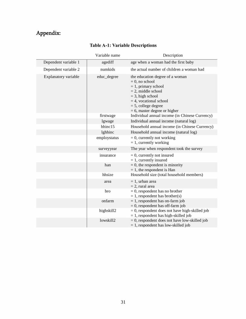
results, women that gave birth at an age younger than 13 years old are dropped. Table A-

1 provides a more detailed description of all controls.

14

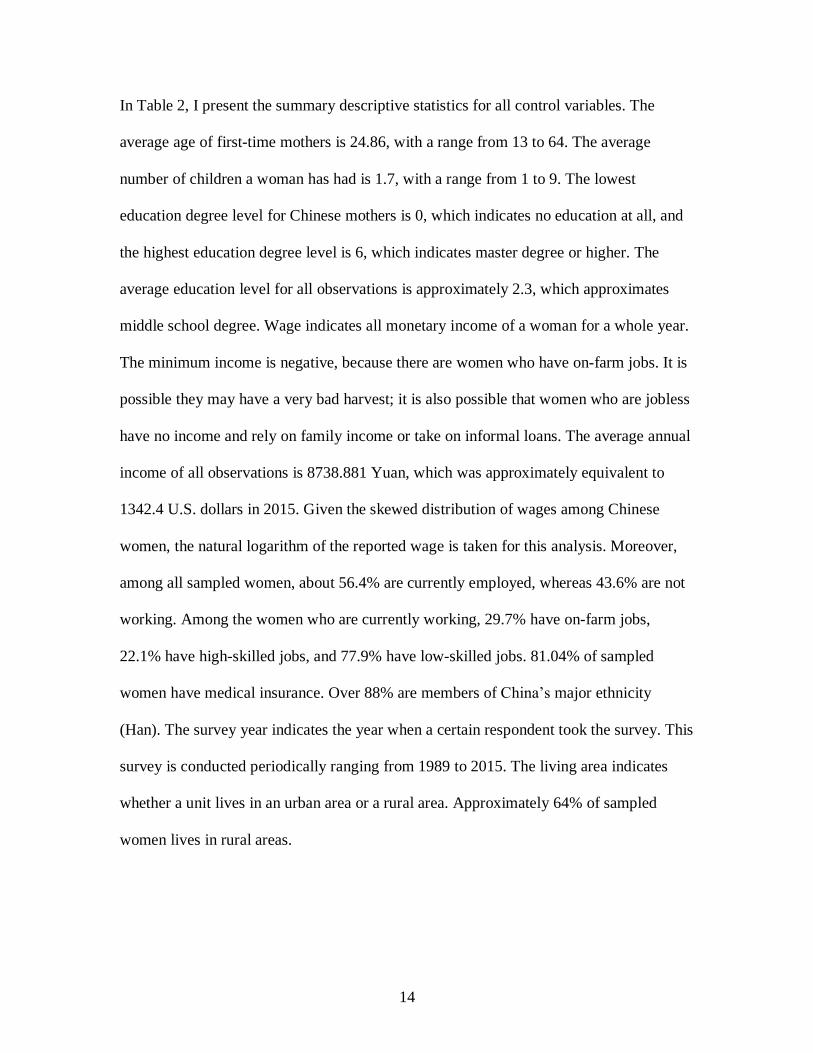
In Table 2, I present the summary descriptive statistics for all control variables. The

average age of first-time mothers is 24.86, with a range from 13 to 64. The average

number of children a woman has had is 1.7, with a range from 1 to 9. The lowest

education degree level for Chinese mothers is 0, which indicates no education at all, and

the highest education degree level is 6, which indicates master degree or higher. The

average education level for all observations is approximately 2.3, which approximates

middle school degree. Wage indicates all monetary income of a woman for a whole year.

The minimum income is negative, because there are women who have on-farm jobs. It is

possible they may have a very bad harvest; it is also possible that women who are jobless

have no income and rely on family income or take on informal loans. The average annual

income of all observations is 8738.881 Yuan, which was approximately equivalent to

1342.4 U.S. dollars in 2015. Given the skewed distribution of wages among Chinese

women, the natural logarithm of the reported wage is taken for this analysis. Moreover,

among all sampled women, about 56.4% are currently employed, whereas 43.6% are not

working. Among the women who are currently working, 29.7% have on-farm jobs,

22.1% have high-skilled jobs, and 77.9% have low-skilled jobs. 81.04% of sampled

women have medical insurance. Over 88% are members of China’s major ethnicity

(Han). The survey year indicates the year when a certain respondent took the survey. This

survey is conducted periodically ranging from 1989 to 2015. The living area indicates

whether a unit lives in an urban area or a rural area. Approximately 64% of sampled

women lives in rural areas.

15

Table 2: Descriptive Statistics on Chinese Mothers from 1995 to 2015

Statistic N Mean St. Dev. Min Max

Employment Status 8,302 0.6 0.5 0.0 1.0

Health Insurance 8,053 0.8 0.4 0.0 1.0

Ethnicity 8,078 0.9 0.3 0.0 1.0

Household Size 8,318 4.0 1.7 1.0 15.0

Household Annual Income 8,319 59,342.0 99,836.5 -679,518.1 4,528,302.0

Number of Children 8,319 1.7 1.0 1 9

Age at First Birth 8,315 24.9 4.2 12.0 64.0

Education Level 7,403 2.3 1.4 0.0 6.0

Living Area 8,319 1.6 0.5 1 2

Individual’s Wage 7,558 8,777.7 22,049.7 -7,200.0 963,000.0

On Farm Job 4,745 0.3 0.5 0.0 1.0

High-Skilled Job 4,727 0.2 0.4 0.0 1.0

Low-Skilled Job 4,727 0.8 0.4 0.0 1.0

Wage(log) 7,557 9.4 0.6 8.6 13.8

Househould income(log) 8,319 13.5 0.2 -3.6 15.5

Note: A complete list of descriptive statistics is provided in Table A-2 in appendix.

4.3 Preliminary Findings

a. The average age of first-time mothers is higher in urban areas than in rural areas

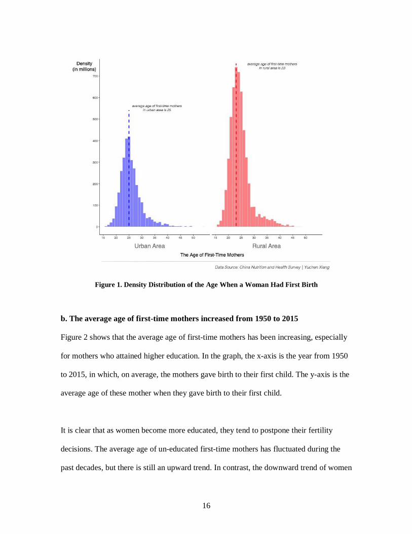
Figure 1 shows the distribution of Chinese women in rural and urban areas and the age

when they had their first child. More women from rural areas than urban areas had at

least one birth, and the average age of first-time mothers is higher in urban areas than in

rural areas (25 versus 23). Such a distribution is certainly encouraging, because before

any formal analysis, my assumption is that women from rural areas would have children

at an earlier age and have more children than women from urban areas.

16

Figure 1. Density Distribution of the Age When a Woman Had First Birth

b. The average age of first-time mothers increased from 1950 to 2015

Figure 2 shows that the average age of first-time mothers has been increasing, especially

for mothers who attained higher education. In the graph, the x-axis is the year from 1950

to 2015, in which, on average, the mothers gave birth to their first child. The y-axis is the

average age of these mother when they gave birth to their first child.

It is clear that as women become more educated, they tend to postpone their fertility

decisions. The average age of un-educated first-time mothers has fluctuated during the

past decades, but there is still an upward trend. In contrast, the downward trend of women

17

who attained Master Degrees and higher started in mid 1980s, probably because the

Chinese government resumed university entrance examinations in 1977, and it took 4

years to finish a bachelor’s degree.

Figure 2. Average Age of First-Time Mothers by Different Education Levels

c. As Chinese women’s education levels increase, their age at first birth increases

Figure 3 shows the distribution of ages of first-time mothers by different education levels.

It is clear that for women who received no education at all, the distribution is very sparse

and contains some outliers; for women who received higher education, the distribution is

more concentrated and contains fewer outliers. The boxplot also shows that as Chinese

women’s education level increases, the age when they first give birth increases. For

example, the mean age of first-time mothers who received primary school education is

24.01 years, but the mean age of first-time mothers who received a Master Degree or

18

higher is 28.26 years. This substantial difference suggests that the effect of education on

Chinese women’s fertility decisions may be statistically significant.

Figure 3. Boxplot Showing Distribution of Chinese Women’s Education Level

4.4 Empirical Results

a. Using age at first birth as dependent variable

In order to test the first hypothesis, the first set of OLS Regressions uses women’s age at

first birth as dependent variable. This set indicates a strong positive correlation between a

woman’s education level and the age when she first gives birth (Table 3). As a woman’s

education level increases, the age when she first gives birth increases, which means that as

education increases, women tend to delay their decisions to have their first child. With

19

more controls added in the model, the coefficient on education is still statistically

significant at the 95% confidence level. Women who live in urban area will have children

later than those in rural area, with a p-value smaller than 0.0001. Holding all else constant,

one unit increase in education degree will lead to a 0.28 increase in the age that a woman

gives birth for the first time; if a woman lives in rural areas, her age when she gives birth

will be 1.043 year younger than a woman who lives in urban areas. Across the regressions

using age at first birth as the dependent variable (Table 3), household size is also a strong

indicator of women’s fertility behavior; women who have a bigger household size will also

give birth earlier.

Verifying the robustness of these findings, negative binomial regressions also produce

highly significant coefficients of education degree and annual income. As I added year

fixed effects and area controls, the results did not vary much and are still significant.

Synthesizing these findings, it becomes apparent that there exists a strong positive

correlation between education and women’s fertility decision. Put differently, Chinese

women at higher levels of education have children later in their life.

20

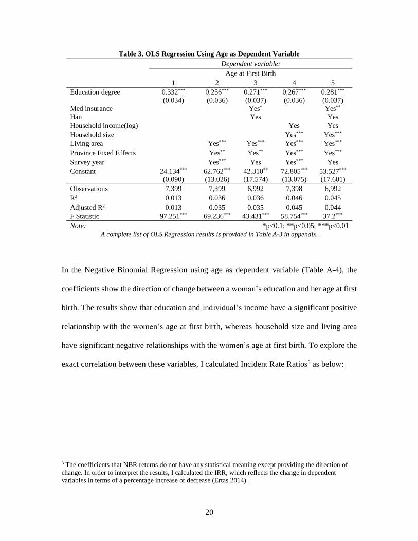
Table 3. OLS Regression Using Age as Dependent Variable Dependent variable: Age at First Birth

1 2 3 4 5

Education degree 0.332*** 0.256*** 0.271*** 0.267*** 0.281*** (0.034) (0.036) (0.037) (0.036) (0.037)

Med insurance Yes* Yes**

Han Yes Yes

Household income(log) Yes Yes

Household size Yes*** Yes***

Living area Yes*** Yes*** Yes*** Yes***

Province Fixed Effects Yes** Yes** Yes*** Yes***

Survey year Yes*** Yes Yes*** Yes

Constant 24.134*** 62.762*** 42.310** 72.805*** 53.527*** (0.090) (13.026) (17.574) (13.075) (17.601)

Observations 7,399 7,399 6,992 7,398 6,992

R2 0.013 0.036 0.036 0.046 0.045

Adjusted R2 0.013 0.035 0.035 0.045 0.044

F Statistic 97.251*** 69.236*** 43.431*** 58.754*** 37.2***

Note: *p<0.1; **p<0.05; ***p<0.01

A complete list of OLS Regression results is provided in Table A-3 in appendix.

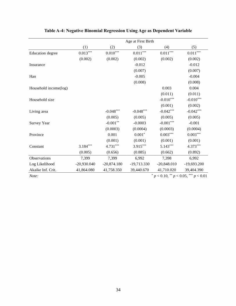
In the Negative Binomial Regression using age as dependent variable (Table A-4), the

coefficients show the direction of change between a woman’s education and her age at first

birth. The results show that education and individual’s income have a significant positive

relationship with the women’s age at first birth, whereas household size and living area

have significant negative relationships with the women’s age at first birth. To explore the

exact correlation between these variables, I calculated Incident Rate Ratios3 as below:

3 The coefficients that NBR returns do not have any statistical meaning except providing the direction of

change. In order to interpret the results, I calculated the IRR, which reflects the change in dependent

variables in terms of a percentage increase or decrease (Ertas 2014).

21

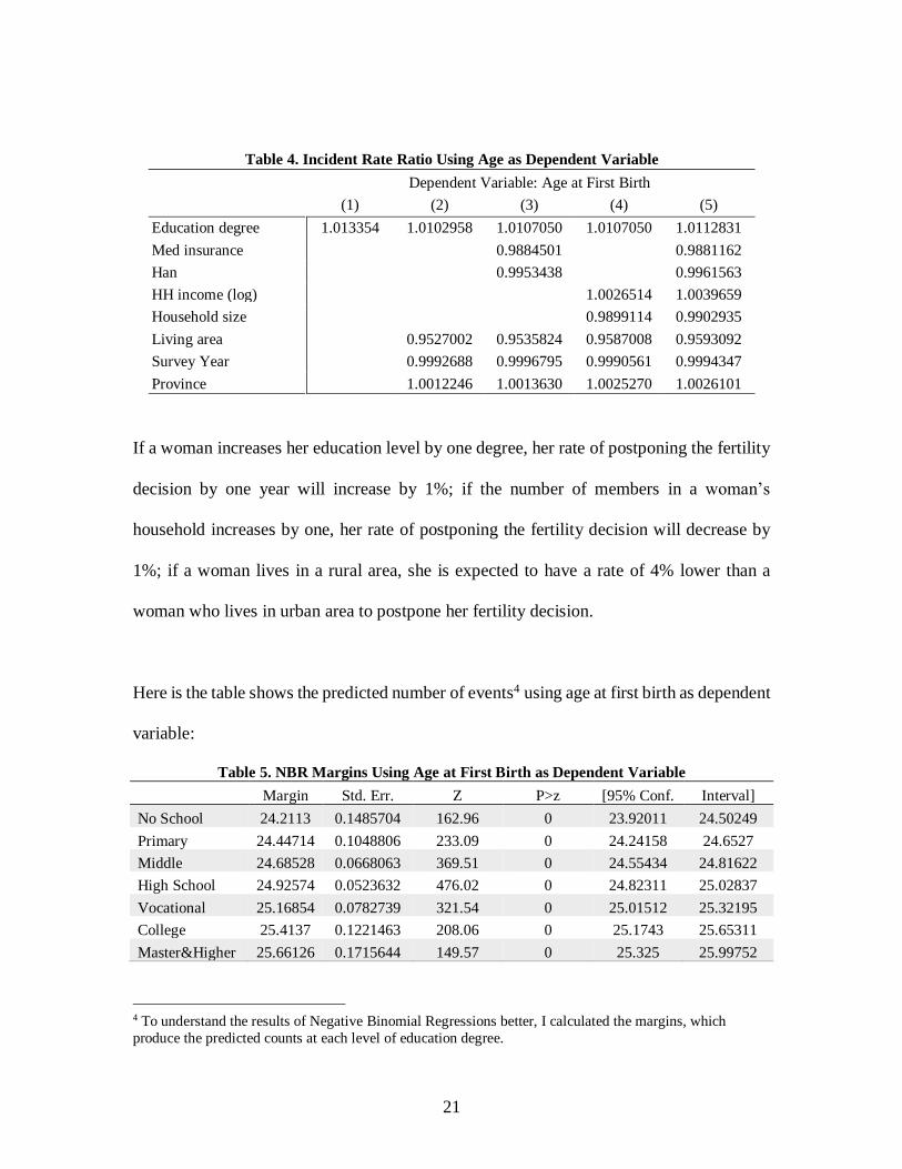
Table 4. Incident Rate Ratio Using Age as Dependent Variable

Dependent Variable: Age at First Birth

(1) (2) (3) (4) (5)

Education degree 1.013354 1.0102958 1.0107050 1.0107050 1.0112831

Med insurance 0.9884501 0.9881162

Han 0.9953438 0.9961563

HH income (log) 1.0026514 1.0039659

Household size 0.9899114 0.9902935

Living area 0.9527002 0.9535824 0.9587008 0.9593092

Survey Year 0.9992688 0.9996795 0.9990561 0.9994347

Province 1.0012246 1.0013630 1.0025270 1.0026101

If a woman increases her education level by one degree, her rate of postponing the fertility

decision by one year will increase by 1%; if the number of members in a woman’s

household increases by one, her rate of postponing the fertility decision will decrease by

1%; if a woman lives in a rural area, she is expected to have a rate of 4% lower than a

woman who lives in urban area to postpone her fertility decision.

Here is the table shows the predicted number of events4 using age at first birth as dependent

variable:

Table 5. NBR Margins Using Age at First Birth as Dependent Variable

Margin Std. Err. Z P>z [95% Conf. Interval]

No School 24.2113 0.1485704 162.96 0 23.92011 24.50249

Primary 24.44714 0.1048806 233.09 0 24.24158 24.6527

Middle 24.68528 0.0668063 369.51 0 24.55434 24.81622

High School 24.92574 0.0523632 476.02 0 24.82311 25.02837

Vocational 25.16854 0.0782739 321.54 0 25.01512 25.32195

College 25.4137 0.1221463 208.06 0 25.1743 25.65311

Master&Higher 25.66126 0.1715644 149.57 0 25.325 25.99752

4 To understand the results of Negative Binomial Regressions better, I calculated the margins, which

produce the predicted counts at each level of education degree.

22

From the table, it is clear that women who obtained master degree or higher gave birth to

their first child at 25.66 years old, whereas women who had no school gave birth to their

first kid at 24.21 years old.

b. Using number of children as dependent variable

In order to examine the second hypothesis, the second set of OLS Regressions uses the

number of children a woman has as dependent variable. The second set indicates a strong

negative correlation between a woman’s education and the number of children she has,

which means that as a woman’s education level increases, she tends to have fewer children.

As I add more controls in this set of regressions, the coefficient on education remains

statistically significant at 1% confidence level. Conversely, the correlation between living

area and number of children is positive: women from rural areas tend to have more children

than women from urban areas. However, indicators including medical insurance, ethnicity,

and household income are not significant factors of a woman’s fertility behavior. In the

OLS Model using the number of children as dependent variable, one level increase in

education degree will lead to a 0.216 decrease in the number of children a woman has had.

Negative Binomial Regressions also indicates that household size can be strong indicators

of fertility behavior, while whether a woman has medical insurance and ethnicity cannot

explain much about Chinese women’s fertility decisions.

23

Table 6. OLS Regression Using Number of Children as Dependent Variable Dependent variable: Number of Children

1 2 3 4 5

Education degree -0.244*** -0.212*** -0.214*** -0.214*** -0.216*** (0.007) (0.007) (0.008) (0.007) (0.008)

Med insurance Yes Yes

Han Yes Yes

Household income(log) Yes Yes

Household size Yes*** Yes***

Living area Yes*** Yes*** Yes*** Yes***

Province Fixed Effects Yes** Yes** Yes*** Yes***

Survey year Yes*** Yes** Yes*** Yes***

Constant 2.155*** -10.361*** -7.649** -11.818*** -9.352** (0.019) (2.694) (3.671) (2.712) (3.686)

Observations 7,403 7,403 6,996 7,402 6,996

R2 0.140 0.175 0.177 0.179 0.181

Adjusted R2 0.140 0.175 0.177 0.178 0.180

F Statistic 1,203.879*** 392.922*** 251.033*** 268.476*** 192.420***

Note: *p<0.1; **p<0.05; ***p<0.01

A complete list of OLS Regression results is provided in Table A-6 in appendix

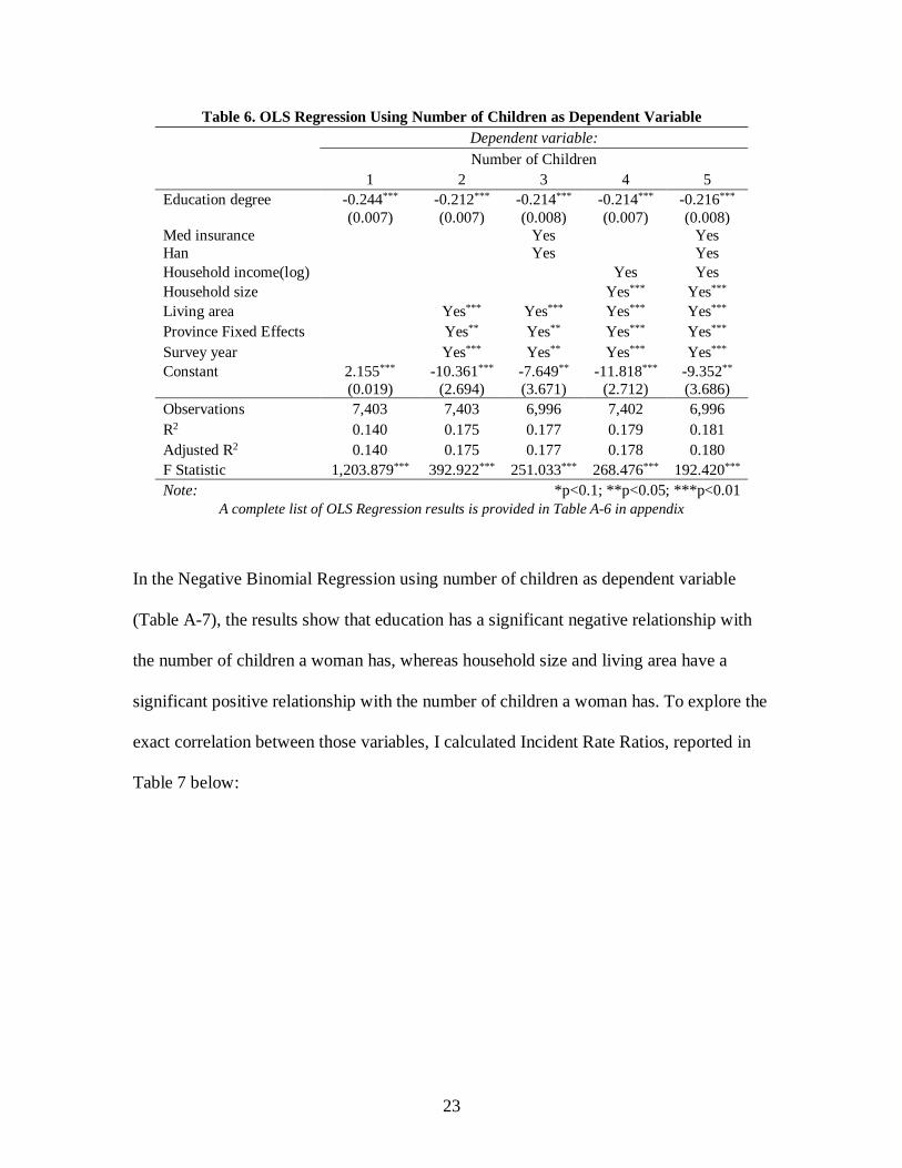
In the Negative Binomial Regression using number of children as dependent variable

(Table A-7), the results show that education has a significant negative relationship with

the number of children a woman has, whereas household size and living area have a

significant positive relationship with the number of children a woman has. To explore the

exact correlation between those variables, I calculated Incident Rate Ratios, reported in

Table 7 below:

24

Table 7. Incident Rate Ratio Using Number of Children as Dependent Variable

Dependent Variable: Number of Children

(1) (2) (3) (4) (5)

Education 0.8505925 0.866699 0.8659994 0.8655538 0.8648681

Med insurance 1.0194339 1.0198657

Han 0.9825622 0.9809703

HH income

(log)

1.003722 1.0081014

Household size 1.020966 1.0197201

Living area 1.159834 1.1594236 1.1449694 1.1456296

Survey year 1.00374 1.0030332 1.0041068 1.0034525

Province 1.026979 1.0270058 1.0241464 1.0243273

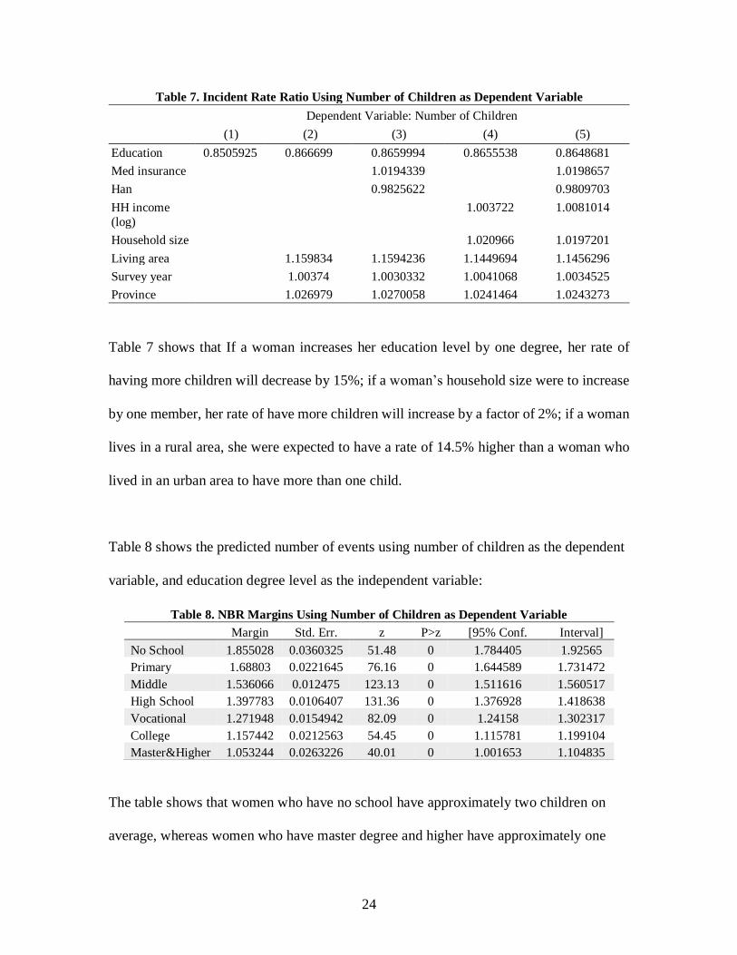
Table 7 shows that If a woman increases her education level by one degree, her rate of

having more children will decrease by 15%; if a woman’s household size were to increase

by one member, her rate of have more children will increase by a factor of 2%; if a woman

lives in a rural area, she were expected to have a rate of 14.5% higher than a woman who

lived in an urban area to have more than one child.

Table 8 shows the predicted number of events using number of children as the dependent

variable, and education degree level as the independent variable:

Table 8. NBR Margins Using Number of Children as Dependent Variable

Margin Std. Err. z P>z [95% Conf. Interval]

No School 1.855028 0.0360325 51.48 0 1.784405 1.92565

Primary 1.68803 0.0221645 76.16 0 1.644589 1.731472

Middle 1.536066 0.012475 123.13 0 1.511616 1.560517

High School 1.397783 0.0106407 131.36 0 1.376928 1.418638

Vocational 1.271948 0.0154942 82.09 0 1.24158 1.302317

College 1.157442 0.0212563 54.45 0 1.115781 1.199104

Master&Higher 1.053244 0.0263226 40.01 0 1.001653 1.104835

The table shows that women who have no school have approximately two children on

average, whereas women who have master degree and higher have approximately one

25

child on average. Such a difference indicates a significant trend between education and

women’s fertility behavior.

c. Instrumental Variable

Since education is likely endogenous, I try to alleviate this issue using an instrumental

variables approach. To be a viable instrument, a variable has to fulfill two criteria. First, it

should be correlated with the treatment variable, in my case, the level of educational

attainment. Previous research shows that the total number of siblings is negatively

associated with an individual’s education attainment level (Lala Carr Steelman 2002). In

China, the preference for boys still exists across the country, so if a woman has brother(s),

her chance of getting education will be lower (Xiaogang Wu 2014). Second, it should not

be related to the outcome variable, i.e., the decision to have children at a later stage in life.

Previous research shows that brothers will have less of an effect in their sisters’ fertility

decisions (Kuziemko 2006). Against this background, I include a dummy variable

indicating whether a woman has brother. This approach can formally be written such that:

𝑋1 = 𝜋0 + 𝜋1𝑍 + 𝜐 (1)

𝑌𝑖 = 𝛽0 + 𝛽1𝑋1 + ∑ 𝛽𝑖𝑋𝑖 + 𝜀𝑖

𝑛

𝑖=2

(2)

Where Z in the first stage equation is the instrumental variable, indicating whether a woman

has brother(s) or not. X1 in the second stage equation is the predicted education level. This

method is used in the univariate regressions (regression 1) and full-control regressions

(regression 5) in both OLS Model 1 and Model 2. I report the results of this regression in

Table 9.

26

Table 9 shows the results between standard OLS regressions and OLS regressions with

instrumental variable, using age at first birth as dependent variable and number of children

as dependent variable. In the regressions using age at first birth as the dependent variable,

the First-Stage F Statistics are 121.94 and 75.44 respectively; in the regressions using

number of children as the dependent variable, the First-Stage F Statistics are 122.03 and

75.54 respectively. Those values are well above the conventional 105, which means that

whether a woman has brother(s) is a strong instrumental variable in indicating this

5 The Rule of Thumb is that if the first stage F < 10, it means the instrumental variables are weak (James H.

Stock 2002).

Table 9: Comparisons between OLS Regressions and OLS with Instrumental Variable

Dependent Variable

Age at First Birth Number of Children

Without IV IV Without IV IV

(1) (5) (1) (5) (1) (5) (1) (5)

Education 0.332*** 0.281*** 0.817*** 0.781** -0.244*** -0.216*** -0.266*** -0.334***

(0.034) (0.037) (3.42) (2.34) (0.007) (0.008) (-7.47) (-6.38)

Insurance -0.296** -0.449* 0.038 0.136***

(0.147) (-1.75) (0.031) (3.30)

Han -0.094 -0.104 -0.050 0.0310

(0.150) (-0.51) (0.031) (0.91)

HH inc (log) 0.095 -0.490 0.016 0.322**

(0.211) (-0.54) (0.044) (2.29)

HH size -0.240*** -0.195*** 0.033*** 0.0749***

(0.030) (-4.79) (0.006) (10.44)

Area -1.043*** -0.989*** 0.201*** -0.0748*

(0.103) (-3.39) (0.022) (-1.69)

Survey year -0.014 0.0408* 0.005*** 0.0155***

(0.009) (1.94) (0.002) (4.53)

Province 0.065*** 0.0686** 0.036*** -0.00589

(0.016) (2.02) (0.003) (-1.15)

Constant 24.13*** 53.53*** 22.85*** -50.03 2.155*** -9.35** 2.05*** -33.62***

(0.090) (17.601) (34.54) (-1.12) (0.019) (3.686) (20.45) (-4.68)

Observations 7,399 6,992 3689 3569 7,403 6,996 3691 3571

R2 0.013 0.045 0.049 0.083 0.140 0.181 -0.009 -0.072

Adjusted R2 0.013 0.044 0.049 0.081 0.140 0.180 -0.009 -0.075

First-Stage F 121.9*** 75.4*** 122.0*** 75.5***

F 97.251*** 37.2*** 11.69 30.77 1,203.9*** 192.4*** 55.73 47.16

Note: * p < 0.10, ** p < 0.05, *** p < 0.01

27

woman’s education level. It is clear that the coefficients of education did not vary much

across the regressions, and it is statistically significant indicator of Chinese women’s

fertility behaviors.

Based on the empirical results, it is clear that Chinese women who live in urban areas and

who obtained higher education tend to have fewer children and have them later; women

who live in rural area and have not received much education are more likely to have more

children and at an earlier age. Since the total resources within a family are limited, the more

children that women have, the less likely it is that all of their children can equally get higher

education. Given that parental preferences for boys are still deeply rooted in Chinese

society, such a situation disadvantages girls who have brothers, because their parents will

probably invest more in their brothers’ education. Thus, my overall results support the

notion that more educated have fewer children at a later stage in life.

5. Policy Implications

Even though the Chinese government replaced the OCP with the SCP, it will not take

long before the country faces a demographic majorly composed of people who have low

levels of human capital. At the end of 2018, there were still no policy reforms that

addressed this issue effectively.

In light of the findings, I would recommend:

1. Introducing a parental leave policy that equally applies to men. In modern China,

gender identity is still a statistically significant factor that negatively influences Chinese

28

women’s labor force participation and earnings, because once women make the fertility

decision, they have to take parental leave, thus incurring a higher operational cost on their

employers (Bing Ye 2018). Given China’s current parental leave policy, women who

obtain higher education and are career-oriented will face workplace discrimination

because of the cost of hiring them. Thus, they will have to postpone their fertility

decisions and have fewer children. Meanwhile, men who obtain the same level of

education do not face such workplace discrimination, because they do not need paid

parental leave or may simply take a very short parental leave, which has a small impact

on their employers’ operation costs. This option results in explicitly discriminatory

questions for females during their job interviews (Stauffer 2018).

Introducing a parental leave policy that equalizes the operational costs of hiring males

and females would eliminate the risk women face of losing their careers if they decide to

have children (OECD 2016). Moreover, women who obtain higher education will have

higher expectations about their children’s educational performance; thus, in the future,

their children will have a much better chance to receive education and to develop high

levels of human capital (Y. Zhang 2011). Therefore, equalizing parental leave policy

would not only promote workplace gender equality, but also incentivize women to have

more children earlier, independent of their educational attainment.

2. Introducing an education policy reform that can reduce cost to women of receiving

education. Another factor that prevents highly educated women from having children is

the opportunity cost incurred by education. In traditional Chinese culture, women are

29

identified as family care providers, and there are still voices that encourage Chinese

women to focus on taking care of their families, and letting men worry about building a

career (Bing Ye 2018). Because, in their traditional view, girls’ getting education is

considered a waste of family resources, women, who are eager to get education, may face

pressure from their families and the society to focus on building a family.

Moreover, previous research shows that access to public education is a strong indicator of

earnings inequality (M.Herrington 2015), which means that women who have limited

education may have a low financial return to the family. Thus, reducing the cost to

women of receiving education will also help to reduce the financial burden of rural

families who live on the poverty line. For example, developing more programs with a

vocational or professional focus particularly for women, and lower the tuition costs of

those programs, so women can get access to education more easily and correspondingly

find jobs more easily. As a result, girls born to these families may have a better chance of

getting education, thus improving her own social status and the overall human capital of

the rural population.

Major resistance to these policies may come from large firms, because they have been

used to avoiding the cost of parental leave by hiring males. The proposed policy shift

would eliminate this option. Another source of resistance may be Chinese men, especially

those who are married, because under the status quo they can use work as an excuse to

avoid doing trivial things like changing diapers, feeding babies, and washing babies’ dirty

30

cloths. Under the proposed policy, Chinese men would have to take equal responsibility

for taking care of babies.

6. Conclusion

Fertility rates in China have been decreasing since the 1970s. Even though the Chinese

government replaced its initial One Child Policy with Second Child Policy, China’s birth

rate dropped from 12.95 per 1,000 people to 10.94 last year. This is the lowest official

birth rate since 1961 (Leng 2019). The objective of this research has been to contribute to

the literature on exploring the mechanism behind Chinese women’s fertility behaviors in

modern society.

My empirical findings indicate that Chinese women who live in urban areas and who

obtain higher education tend to have fewer children and have them later. Conversely,

women who live in rural areas and do not have much education are more likely to have

more children and at an earlier age. Additionally, Chinese women who have brothers will

obtain a lower education level, thus being more likely to have more children and have

them earlier.

As a society develops to a stage where farming is no longer a major source of income for

most families, and jobs increasingly require mental labor instead of physical labor,

women will become as competitive as men in labor market. Preference for boys is rapidly

becoming an outdated prejudice. Chinese women have been fighting against this

prejudice for too long. Thus, reforms in parental leave policy and education policy are

necessary, not just to address the aging issue and promote birth rates among people with

high human capital level, but also to promote the rights that women deserve.

31

Appendix:

Table A-1: Variable Descriptions

Variable name Description

Dependent variable 1 agediff age when a woman had the first baby

Dependent variable 2 numkids the actual number of children a woman had

Explanatory variable educ_degree the education degree of a woman

= 0, no school

= 1, primary school

= 2, middle school

= 3, high school

= 4, vocational school

= 5, college degree

= 6, master degree or higher

firstwage Individual annual income (in Chinese Currency)

lgwage Individual annual income (natural log)

hhinc15 Household annual income (in Chinese Currency)

lghhinc Household annual income (natural log)

employstatus = 0, currently not working

= 1, currently working

surveyyear The year when respondent took the survey

insurance = 0, currently not insured

= 1, currently insured

han = 0, the respondent is minority

= 1, the respondent is Han

hhsize Household size (total household members)

area = 1, urban area

= 2, rural area

bro = 0, respondent has no brother

= 1, respondent has brother(s)

onfarm = 1, respondent has on-farm job

= 0, respondent has off-farm job

highskill2 = 0, respondent does not have high-skilled job

= 1, respondent has high-skilled job

lowskill2 = 0, respondent does not have low-skilled job

= 1, respondent has low-skilled job

32

Table A-2: Descriptive Statistics on Chinese Mothers from 1989 to 2015

Statistic N Mean St. Dev. Min Max

Employment Status 8,302 0.6 0.5 0.0 1.0

Survey Year 8,319 2,010.1 7.2 1,989 2,015

Health Insurance 8,053 0.8 0.4 0.0 1.0

Ethnicity 8,078 0.9 0.3 0.0 1.0

Household Size 8,318 4.0 1.7 1.0 15.0

Household Annual Income 8,319 59,342.0 99,836.5 -679,518.1 4,528,302.0

Number of Children 8,319 1.7 1.0 1 9

Age at First Birth 8,315 24.9 4.2 12.0 64.0

Education Level 7,403 2.3 1.4 0.0 6.0

Living Area 8,319 1.6 0.5 1 2

Individual's Wage 7,558 8,777.7 22,049.7 -7,200.0 963,000.0

On Farm Job 4,745 0.3 0.5 0.0 1.0

Wage(log) 7,557 9.4 0.6 8.6 13.8

Household income(log) 8,319 13.5 0.2 -3.6 15.5

Has brother 3,844 0.7 0.5 0.0 1.0

High-Skilled Job 4,727 0.2 0.4 0.0 1.0

Low-Skilled Job 4,727 0.8 0.4 0.0 1.0

Province 8,319 6.8 3.2 1 12

33

Table A-3: OLS Regression Using Age as Dependent Variable

Age at First Birth

(1) (2) (3) (4) (5)

Education degree 0.332*** 0.256*** 0.271*** 0.267*** 0.281***

(0.034) (0.036) (0.037) (0.036) (0.037)

Insurance -0.288* -0.296**

(0.147) (0.147)

Han -0.116 -0.094

(0.151) (0.150)

Household Income(log) 0.064 0.095

(0.211) (0.211)

Household size -0.250*** -0.240***

(0.029) (0.030)

Living area -1.215*** -1.191*** -1.059*** -1.043***

(0.099) (0.102) (0.100) (0.103)

Survey year -0.018*** -0.008 -0.023*** -0.014

(0.007) (0.009) (0.007) (0.009)

Province 0.030** 0.034** 0.063*** 0.065***

(0.015) (0.015) (0.015) (0.016)

Constant 24.134*** 62.762*** 42.310** 72.805*** 53.527***

(0.090) (13.026) (17.574) (13.075) (17.601)

Observations 7,399 7,399 6,992 7,398 6,992

R2 0.013 0.036 0.036 0.046 0.045

Adjusted R2 0.013 0.035 0.035 0.045 0.044

F Statistic 97.251*** 69.236*** 43.431*** 58.754*** 37.2***

Note * p < 0.10, ** p < 0.05, *** p < 0.01

34

Table A-4: Negative Binomial Regression Using Age as Dependent Variable

Age at First Birth

(1) (2) (3) (4) (5)

Education degree 0.013*** 0.010*** 0.011*** 0.011*** 0.011***

(0.002) (0.002) (0.002) (0.002) (0.002)

Insurance -0.012 -0.012

(0.007) (0.007)

Han -0.005 -0.004

(0.008) (0.008)

Household income(log) 0.003 0.004

(0.011) (0.011)

Household size -0.010*** -0.010***

(0.001) (0.002)

Living area -0.048*** -0.048*** -0.042*** -0.042***

(0.005) (0.005) (0.005) (0.005)

Survey Year -0.001** -0.0003 -0.001*** -0.001

(0.0003) (0.0004) (0.0003) (0.0004)

Province 0.001 0.001* 0.003*** 0.003***

(0.001) (0.001) (0.001) (0.001)

Constant 3.184*** 4.731*** 3.915*** 5.143*** 4.373***

(0.005) (0.656) (0.885) (0.662) (0.892)

Observations 7,399 7,399 6,992 7,398 6,992

Log Likelihood -20,930.040 -20,874.180 -19,713.330 -20,848.010 -19,693.200

Akaike Inf. Crit. 41,864.080 41,758.350 39,440.670 41,710.020 39,404.390

Note: * p < 0.10, ** p < 0.05, *** p < 0.01

35

Table A-6: OLS Regression Using Number of Children as Dependent Variable

Number of Children

(1) (2) (3) (4) (5)

Education degree -0.244*** -0.212*** -0.214*** -0.214*** -0.216***

(0.007) (0.007) (0.008) (0.007) (0.008)

Insurance 0.037 0.038

(0.031) (0.031)

Han -0.047 -0.050

(0.031) (0.031)

Household Income(log) 0.009 0.016

(0.044) (0.044)

Household size 0.035*** 0.033***

(0.006) (0.006)

Living area 0.221*** 0.221*** 0.200*** 0.201***

(0.020) (0.021) (0.021) (0.022)

Survey year 0.006*** 0.005** 0.007*** 0.005***

(0.001) (0.002) (0.001) (0.002)

Province 0.040*** 0.040*** 0.036*** 0.036***

(0.003) (0.003) (0.003) (0.003)

Constant 2.155*** -10.361*** -7.649** -11.818*** -9.352**

(0.019) (2.694) (3.671) (2.712) (3.686)

Observations 7,403 7,403 6,996 7,402 6,996

R2 0.140 0.175 0.177 0.179 0.181

Adjusted R2 0.140 0.175 0.177 0.178 0.180

F Statistic 1,203.879*** 392.922*** 251.033*** 268.476*** 192.420***

Note * p < 0.10, ** p < 0.05, *** p < 0.01

36

Table A-7: NBR Using Number of Children as Dependent Variable

Number of Children

(1) (2) (3) (4) (5)

Education degree -0.162*** -0.143*** -0.144*** -0.144*** -0.145***

(0.007) (0.008) (0.008) (0.008) (0.008)

Insurance 0.019 0.020

(0.030) (0.030)

Han -0.018 -0.019

(0.029) (0.029)

Household income(log) 0.004 0.008

(0.042) (0.043)

Household size 0.021*** 0.020***

(0.006) (0.006)

Living area 0.148*** 0.148*** 0.135*** 0.136***

(0.020) (0.021) (0.021) (0.021)

Survey year 0.004*** 0.003* 0.004*** 0.003*

(0.001) (0.002) (0.001) (0.002)

Province 0.027*** 0.027*** 0.024*** 0.024***

(0.003) (0.003) (0.003) (0.003)

Constant 0.814*** -7.155*** -5.734 -7.981*** -6.720*

(0.017) (2.611) (3.608) (2.630) (3.624)

Observations 7,403 7,403 6,996 7,402 6,996

Log Likelihood -9,830.125 -9,758.017 -9,244.010 -9,749.817 -9,238.203

Akaike Inf. Crit. 19,664.250 19,526.030 18,502.020 19,513.630 18,494.410

Note: * p < 0.10, ** p < 0.05, *** p < 0.01

37

Table A-8: OLS Sub-Regressions Between Employed and Unemployed Women

Dependent variable:

Age at First Birth Number of Children

Employed Unemployed Employed Unemployed

Education degree 0.461*** -0.072 -0.199*** -0.241***

(0.040) (0.074) (0.009) (0.015)

Insurance 0.090 -0.821*** -0.067* 0.177***

(0.162) (0.284) (0.036) (0.058)

Han -0.122 -0.451 -0.095*** -0.108*

(0.163) (0.282) (0.036) (0.057)

Household income(log) 0.354 0.052 -0.293** 0.052

(0.625) (0.254) (0.138) (0.052)

Household size -0.179*** -0.213*** 0.050*** 0.055***

(0.035) (0.049) (0.008) (0.010)

Survey year -0.012 -0.058*** 0.005** 0.002

(0.009) (0.021) (0.002) (0.004)

Living area -0.942*** -1.093*** 0.131*** 0.265***

(0.117) (0.183) (0.026) (0.037)

Constant 44.286** 143.873*** -4.463 -2.780

(18.338) (41.413) (4.050) (8.424)

Observations 4,094 2,885 4,097 2,886

R2 0.082 0.041 0.181 0.137

Adjusted R2 0.080 0.039 0.180 0.135

Residual Std. Error 3.400

(df = 4086)

4.538

(df = 2877)

0.751

(df = 4089)

0.923

(df = 2878)

F Statistic 51.867***

(df = 7; 4086)

17.622***

(df = 7; 2877)

129.214***

(df = 7; 4089)

65.071***

(df = 7; 2878)

Note: * p < 0.10, ** p < 0.05, *** p < 0.01

38

Table A-9: OLS Sub-Regressions Between High-Skilled Job and Low-Skilled Job

Dependent variable:

Age at First Birth Number of Children

High-Skilled Low-Skilled High-Skilled Low-Skilled

Education degree 0.328*** 0.233*** -0.055*** -0.201***

(0.085) (0.057) (0.012) (0.013)

Income(log) 0.534*** 0.800*** -0.090*** -0.258***

(0.161) (0.131) (0.023) (0.031)

Insurance 0.662* -0.008 -0.045 -0.129***

(0.347) (0.195) (0.050) (0.046)

Han (reference: minority) 0.144 -0.245 0.010 -0.042

(0.342) (0.191) (0.049) (0.045)

Household income(log) 0.237 -0.215 0.024 -0.252

(0.929) (0.860) (0.134) (0.201)

Household size -0.175** -0.171*** 0.041*** 0.059***

(0.070) (0.041) (0.010) (0.010)

Survey year -0.036** -0.038*** 0.003 0.013***

(0.017) (0.012) (0.002) (0.003)

Living area -1.131*** -0.746*** 0.059* 0.106***

(0.211) (0.144) (0.031) (0.034)

Constant 89.262*** 98.117*** -4.729 -19.412***

(32.644) (24.230) (4.714) (5.659)

Observations 947 3,040 947 3,043

R2 0.125 0.057 0.112 0.189

Adjusted R2 0.117 0.054 0.105 0.186

Residual Std. Error 2.964

(df = 938)

3.535

(df = 3031)

0.428

(df = 938)

0.826

(df = 3034)

F Statistic 16.721***

(df = 8; 938)

22.730***

(df = 8; 3031)

14.839***

(df = 8; 938)

88.172***

(df = 8; 3034)

Note: * p < 0.10, ** p < 0.05, *** p < 0.01

39

References

Barnes, Hannah. BBC News. 9 18, 2013. https://www.bbc.com/news/magazine-

24128176.

Bing Ye, Yucong Zhao. Women hold up half the sky? Gender identity and the wife's

labor market performance in China. China Economic Review, 2018.

C.G. Swicegood, F.D. Bean. Immigrant Fertility. International Encyclopedia of the

Social & Behavioral Sciences, 2001.

China Labor Bulletin. April 2018. https://clb.org.hk/content/workplace-discrimination.

Ertas, Nevbahar. Political Voice and Civic Attentiveness of Public and Non-Profit

Employees. The American Review of Public Administration, 2014.

Fang, Hai, Karen N Eggleston, John A Rizzo, and Richard J Zackhauser. Jobs and Kids:

Female Employment and Fertility in China. HKS Faculty Research Working

Paper, 2012.

Garcia, Jorge Luis. Fertility after China’s More-than-One-Child Policy. The University

of Chicago, 2017.

Hai Fang, Karen N. Eggleston, John A. Rizzo, Richard J. Zeckhauser. Jobs and Kids:

Female Employment and Fertility in China. HKS Faculty Research Working

Paper, 2012.

James H. Stock, Jonathan H. Wright, Motohiro Yogo. A Survey of Weak Instruments and

Weak Identification in Generalized Method of Moments. Journal of Business &

Economic Statistics, 2002.

Kuziemko, Ilyana. Is Having Babies Contagious? Estimating Fertility Peer Effects

Between Siblings. Harvard University, 2006.

Lala Carr Steelman, Brian Powell, Regina Werum, Scott Carter. Reconsidering the

Effects of Sibling Configuration: Recent Advances and Challenges. Annual

Review of Sociology, 2002.

Leng, Sidney. China’s birth rate falls again, with 2018 producing the fewest babies since

1961, official data shows. Jan 21, 2019. https://www.scmp.com/economy/china-

economy/article/2182963/chinas-birth-rate-falls-again-2018-producing-fewest-

babies.

40

M.Herrington, Christopher. Public education financing, earnings inequality, and

intergenerational mobility. Review of Economic Dynamics, 2015.

Numbeo. 2018. https://www.numbeo.com/cost-of-

living/country_result.jsp?country=China.

OECD. Parental leave: Where are the fathers? OECD, 2016.

Stauffer, Brian. Map Video “Only Men Need Apply” Gender Discrimination in Job

Advertisements in China. Human Rights Watch, 2018.

UCLA. Institute for Digital Research & Education. 2019.

https://stats.idre.ucla.edu/stata/dae/negative-binomial-regression/?cv=1 (accessed

April 11, 2019).

Xiaogang Wu, Hua Ye, Gloria Guangye He. "Fertility Decline and Women’s Status

Improvement in China." (Population Studies Center Research Report 14-812)

2014.

Xuebo Wang, Junsen Zhang. Beyond the Quantity–Quality tradeoff: Population control

policy and human capital investment. Journal of Development Economics, 2018.

Yue Qian, Yongai Jin. Women’s Fertility Autonomy in Urban China: The Role of Couple

Dynamics Under the Universal Two-Child Policy. Chinese Sociological Review,

2018.

Zhang, Junsen. Socioeconomic Determinants of Fertility in China a Microeconometric

Analysis. Journal of Population Economics, 1990.

Zhang, Junsen. The Evolution of China’s One-Child Policy and Its Effects on Family

Outcomes. Journal of Economic Perspectives, 2017.

Zhang, Yuping. Mothers' Educational Expectations and Children's Enrollment: Evidence

from Rural China. University of Pennsylvania ScholarlyCommons, 2011.