The contact zone of the grass snake (Natrix natrix in … CONTACT ZONE OF THE GRASS SNAKE (NATRIX...
99
Institut de Biologie Rue Emile-Argand 11 CH – 2000 Neuchâtel MASTER THESIS under the supervision of Dr. Sylvain Ursenbacher Juin 2015 Maxime Chèvre The contact zone of the grass snake (Natrix natrix) in Switzerland
-
Upload
phunghuong -
Category
Documents
-
view
230 -
download
5
Transcript of The contact zone of the grass snake (Natrix natrix in … CONTACT ZONE OF THE GRASS SNAKE (NATRIX...
Institut de Biologie
Rue Emile-Argand 11
CH – 2000 Neuchâtel
MASTER THESIS
under the supervision of
Dr. Sylvain Ursenbacher
Juin 2015
Maxime Chèvre
The contact zone of the
grass snake (Natrix natrix)
in Switzerland

THE CONTACT ZONE OF THE GRASS SNAKE (NATRIX NATRIX) IN SWITZERLAND 2013 – 2015 1
CONTENTS
RÉSUMÉ --------------------------------------------------------------------------------------------------------------------------- 3
ABSTRACT ------------------------------------------------------------------------------------------------------------------------ 4
FIRST PART ----------------------------------------------------------------------------------------------------------------------- 5
INTRODUCTION -------------------------------------------------------------------------------------------------------------- 5 1. Introduction ------------------------------------------------------------------------------------------------------------------ 6
1.1. Species concepts ------------------------------------------------------------------------------------------------------------- 6 1.1.1. A Taxonomy in crisis? ------------------------------------------------------------------------------------------------ 6 1.1.2. Biological species concept (BSC) ----------------------------------------------------------------------------------- 6 1.1.3. Phylogenetic species concept (PSC) ------------------------------------------------------------------------------- 7 1.1.4. Evolutionary species concept (ESC) ------------------------------------------------------------------------------- 8 1.1.5. Emergent concepts---------------------------------------------------------------------------------------------------- 9
1.2. Subspecies concept-------------------------------------------------------------------------------------------------------- 11 1.3. The grass snake ------------------------------------------------------------------------------------------------------------ 13 1.4. Hybrid zone and phylogeography of the grass snake subspecies ------------------------------------------------ 14 1.5. The Red Lists --------------------------------------------------------------------------------------------------------------- 16 1.6. Genetic markers and morphology -------------------------------------------------------------------------------------- 18 1.7. Aims of the study ---------------------------------------------------------------------------------------------------------- 21
PART TWO ---------------------------------------------------------------------------------------------------------------------- 24
MATERIALS AND METHODS --------------------------------------------------------------------------------------------- 24 2. Material and methods ---------------------------------------------------------------------------------------------------- 25
2.1. Study area and origin of the samples ---------------------------------------------------------------------------------- 25 2.2. Laboratory procedures --------------------------------------------------------------------------------------------------- 26
2.2.1. DNA purification ---------------------------------------------------------------------------------------------------- 26 2.2.2. Mitochondrial DNA amplification and sequencing ----------------------------------------------------------- 26 2.2.3. Microsatellites amplification and sequencing ----------------------------------------------------------------- 27
2.3. Genetic data analyses ----------------------------------------------------------------------------------------------------- 27 2.3.1. Mitochondrial DNA ------------------------------------------------------------------------------------------------- 27 2.3.2. Microsatellites ------------------------------------------------------------------------------------------------------- 28
2.4. Morphological data acquisition ----------------------------------------------------------------------------------------- 30 2.4.1. Criteria selection ---------------------------------------------------------------------------------------------------- 30 2.4.2. Morphological measurements ------------------------------------------------------------------------------------ 31 2.4.3. Geometric morphometrics ---------------------------------------------------------------------------------------- 31
2.5. Morphological data treatments ----------------------------------------------------------------------------------------- 33 2.5.1. Univariate analyses ------------------------------------------------------------------------------------------------- 33 2.5.2. Multivariate analyses ----------------------------------------------------------------------------------------------- 34 2.5.3. Landmark-based geometric morphometric-------------------------------------------------------------------- 35
2.6. Geographic information system (GIS) --------------------------------------------------------------------------------- 35
PART THREE -------------------------------------------------------------------------------------------------------------------- 36
RESULTS --------------------------------------------------------------------------------------------------------------------- 36 3. Results ----------------------------------------------------------------------------------------------------------------------- 37
3.1. Mitochondrial DNA -------------------------------------------------------------------------------------------------------- 37 3.2. Microsatellites ------------------------------------------------------------------------------------------------------------- 39
3.2.1. Population structure------------------------------------------------------------------------------------------------ 39 3.2.2. Population-based analysis----------------------------------------------------------------------------------------- 42 3.2.3. Relatedness between individuals -------------------------------------------------------------------------------- 43
3.3. Morpholgy ------------------------------------------------------------------------------------------------------------------ 45 3.3.1. Univariate analyses ------------------------------------------------------------------------------------------------- 45 3.3.2. Multivariate analyse ------------------------------------------------------------------------------------------------ 45 3.3.3. Geometric morphometric ------------------------------------------------------------------------------------------ 50
PART FOUR --------------------------------------------------------------------------------------------------------------------- 52
DISCUSSION ----------------------------------------------------------------------------------------------------------------- 52 3.4. Gene flow in the contact zone ------------------------------------------------------------------------------------------- 53 3.5. Morphology ----------------------------------------------------------------------------------------------------------------- 58 3.6. Taxonomic reassessment ------------------------------------------------------------------------------------------------ 61 3.7. Next Red List of reptiles of Switzerland and conservation implications --------------------------------------- 62

THE CONTACT ZONE OF THE GRASS SNAKE (NATRIX NATRIX) IN SWITZERLAND 2013 – 2015 2
3.8. Perspective ----------------------------------------------------------------------------------------------------------------- 63
PART FIVE ----------------------------------------------------------------------------------------------------------------------- 66
CONCLUSION ---------------------------------------------------------------------------------------------------------------- 66 3.8.1. Acknowledgments -------------------------------------------------------------------------------------------------- 69
PART SIX ------------------------------------------------------------------------------------------------------------------------ 70
BIBLIOGRAPHY ------------------------------------------------------------------------------------------------------------- 70
PART SEVEN -------------------------------------------------------------------------------------------------------------------- 76
ANNEXES -------------------------------------------------------------------------------------------------------------------- 76
THE CONTACT ZONE OF THE GRASS SNAKE (NATRIX NATRIX) IN SWITZERLAND 2013 – 2015 3
Résumé
Actuellement, deux sous-espèces de couleuvre à collier sont reconnues en Suisse : Natrix natrix natrix
présente au nord-est de la Suisse et Natrix natrix helvetica présente dans le reste du territoire. La
première est classée « en danger » selon la Liste Rouge tandis que la seconde appartient à la catégorie «
vulnérable ». Dans la Liste Rouge des reptiles de Suisse 2005, l’utilisation de l’unité infraspécifique
«sous-espèce » a été retenue pour cette espèce, se basant exclusivement sur des données
morphologiques.
De récentes études génétiques basées sur des gènes mitochondriaux suggèrent que ces deux sous-
espèces se seraient séparées il y a 7 millions d’années déjà. Cette séparation, certes ancienne, ne les a
pas conduites à évoluer de manière à présenter des différences morphologiques importantes qui
permettraient une identification facile et assurée de la sous-espèce. Cependant, nos connaissances
actuelles concernant la morphologie de l’espèce datent des années 1970-1980 et sont relativement peu
approfondies pour la Suisse.
Afin de réévaluer la validité de leurs statuts de sous-espèces en combinant plusieurs techniques
récentes, une étude génétique basée sur 195 individus de Suisse a été menée. Deux gènes
mitochondriaux ont été séquencés pour connaître la répartition des différents haplotypes ainsi que leur
diversité. En complément, l’ADN nucléaire a été étudié à l’aide de 13 marqueurs microsatellites afin
d’évaluer la structure génétique de cette zone de contact, notamment pour connaître la nature du flux de
gènes entre de ces deux taxa. En parallèle, des analyses morphologiques ont également été menées afin
d’évaluer la possibilité future de discriminer ces deux groupes sans avoir recours à la génétique.
Les résultats indiquent que le flux de gènes est extrêmement réduit entre les deux sous-espèces, avec la
détection d’individus hybrides sur une bande restreinte d’environ 10 km de largeur. Ces observations
indique l’existence de deux taxa isolés qui pourraient donc être considérés comme des espèces
différentes. Les analyses morphologiques indiquent elles aussi des différences assez claires pour
quelques critères (taille des taches dorsales latérales, forme et taille du « collier » et certaines
proportions du corps), permettant une discrimination des deux taxa avec un certain niveau de confiance.

THE CONTACT ZONE OF THE GRASS SNAKE (NATRIX NATRIX) IN SWITZERLAND 2013 – 2015 4
Abstract
Currently, two grass snake subspecies are recognised in Switzerland: Natrix natrix natrix in northeast
part of the Switzerland and Natrix natrix helvetica in the rest of the country. According to the last Red
List of the reptiles of Switzerland dated 2005, N. n. natrix is listed as “endangered” and N. n. helvetica
as “vulnerable”. The infraspecific taxonomic level chosen in these threat evaluations for this species is
based exclusively on morphological data.
Recent phylogenetic studies based on mitochondrial genes suggest that these subspecies started their
divergence 7 millions years ago. However, despite this ancient separation, their evolution does not
conduct them to a clear morphological differentiation and their discrimination is not totally ensured.
However, all the existing knowledge is based on studies conducted in the seventies and the eighties and
could be more detailed in Switzerland.
In order to reassess the validity of their subspecies status, using several recent technics, a genetic study
based on 195 Swiss individuals was conducted. Two mitochondrial genes were sequenced to assess the
repartition and the diversity of the different haplotypes. Additionally the nuclear DNA was analysed
with 13 microsatellites to evaluate the genetic structure at the contact zone and to observe the nature of
the gene flow between both taxa. In parallel, morphological analyses was conducted to evaluate the
future possibility to discriminate these taxa without molecular tools.
The results show a reduced gene flow between both subspecies with the identification of hybrids along
a strip 10 km wide. This genetic isolation suggests the possibility to recognise these taxa as separate
species. Finally, morphological analyses showed the likelihood of discriminating these taxa when
several criteria are used (lateral blotches size and length, nuchal marking length and shape and other
body proportions).

THE CONTACT ZONE OF THE GRASS SNAKE (NATRIX NATRIX) IN SWITZERLAND 2013 – 2015 5
First part
INTRODUCTION
THE CONTACT ZONE OF THE GRASS SNAKE (NATRIX NATRIX) IN SWITZERLAND 2013 – 2015 6
1. INTRODUCTION
1.1. SPECIES CONCEPTS
1.1.1. A Taxonomy in crisis?
Questions around the definition and the understanding of the species are still under a heated
debate and constitute a discipline of biology itself. Concepts defining the species are abundant
and are all developed for the same purpose: to delineate the boundaries of biological units in
view to describe and class the diversity of life. The species are considered to be the most
important unit for taxonomy: in a metaphor, Cracraft (2000) described them as the
“systematics’ elementary particles”. Unfortunately, despite this widely accepted idea, the
taxonomy is going through a crisis due to numerous concepts, often discordant, trying to
describe the biological diversity (Dayrat 2005, de Queiroz 2007). The resulting problem is the
difficulty to work with an “elementary particle” defined by many definitions affecting many
disciplines as evolutionary biology, ecology, conservation, policy decisions, industry (as
pharmacology), medicine, etc (Hey et al. 2003, Dayrat 2005).
It becomes necessary to have efficient tools to describe the life’s diversity on earth, especially
for conservation purposes (linked to the increasing human pressure on the environment). In this
way, a general consensus around the species definition is necessary (Dayrat 2005, Padial et al.
2010) in order to have a good estimation and inventory of the biodiversity. For De Queiroz
(2007) this unique consensual species concept could be not so unreachable as expected and the
crisis not so serious as it appears.
Three concepts can be identified as the most accepted and used today: the biological species
concept (BSC), the phylogenetic species concept (PSC) and the evolutionary species concept
(ESC) (Frankham et al. 2012). Bellow, the chapter Species concepts will detailed these
principal concepts and their critics, but also emergent ideas as the “differential fitness species
concept” or the “integrative taxonomy”.
1.1.2. Biological species concept (BSC)
This concept was firstly developed by Dobzhansky and Mayr in the first part of the 20th
century
and species can be resumed as “groups of actually or potentially interbreeding natural
populations, which are reproductively isolated from other such groups” (Mayr 1942). The BSC
focuses on the reproductive isolation of populations induced by internal or physiological
mechanisms (excluding geographic isolation). In the example of two species represented by
THE CONTACT ZONE OF THE GRASS SNAKE (NATRIX NATRIX) IN SWITZERLAND 2013 – 2015 7
two populations of individuals, it means that the gene flow (ability of the genes to move
spatially allowing formation of harmonious gene pool in groups of organisms) occurs within
each population but is interrupted between the two species by intrinsic mechanisms. Despite
this major advance in the species definition, many critics have been argued against this
concept. The first major critic comes from the difficulties to highlight the reproductive
isolation of allopatric populations (i.e. geographically separated populations) regarded as
distinct species. The reproductive isolation can only be suspected and sometimes impossible to
demonstrate with scientific and objective evidences. Another condition of the BSC under
critics frequently mentioned is that interspecific hybridization is not possible (or resultant
offspring are not viable or fertile). Under the BSC, if two species can produce fertile offspring,
then they have to be considered as subspecies or semi-species. However, incomplete
reproductive isolation (i.e. semipermeable barrier to the gene flow) between recognized species
is widely found in the nature (Mallet 2005, Hey and Pinho 2012, Hausdorf 2011, Groves and
Grubb 2011, Frankham et al. 2012,). In a literature survey, Mallet (2005) found that 25% of the
vascular plant species in UK, 6 % of the European mammals and 9% of the birds in the world
(the mean is around 10% of the animals in the world) hybridize in the nature, especially for
young species. The last criticism considered here, highlighted by several studies simulation-
based (see Petit and Excoffier 2009), is that gene flow could not totally explain the genetic
homogeneity between populations within the same species. Conversely, the interspecific gene
flow is too important to keep species well differentiated. For Petit and Excoffier (2009), the
selective pressure (e.g. induced by the environment) is an important cofactor able to solve the
problems induced by semipermeable barrier to the gene flow. To sum up, a species concept
based exclusively on reproductive isolation seem omit other important phenomenon occurring
in speciation with a risk to underestimate entities presenting a real evolutionary interest.
1.1.3. Phylogenetic species concept (PSC)
As for the BSC, there is no unique definition of the phylogenetic species concept (PSC). Here,
I will present the diagnosable phylogenetic concept as defined by Cracraft (1989): “A species is
an irreducible (basal) cluster of organisms, diagnosably distinct from other such clusters, and
within which there is a parental pattern of ancestry and descent”. The diagnosable version of
the PSC does not need a strict recognition of monophyletic lineage, this point seems important
as introgression (Mallet 2005) and reticulation (species formed by hybridisation) can also occur
in speciation mechanism. Explained by Mallet (2006), this concept considers species as a
population of individuals with fixed differences. These fixed differences have to be 100%
THE CONTACT ZONE OF THE GRASS SNAKE (NATRIX NATRIX) IN SWITZERLAND 2013 – 2015 8
diagnosable, for example shared mutations in DNA sequences or morphological traits. This
concept focuses on the evolutionary relationship among organisms, where species can be seen
as terminal branches of a cladogram (graphic representation in tree structure of the
evolutionary links between species) represented by an ancestral–descendant sequence.
The concept is based only on data readily available and not at all on mechanism and/or
consequence of speciation such as reproductive isolation. Thus it is applicable for allopatric
populations and for asexual organism where BSC presents difficulties. However, this concept
is not immune to criticism as small isolated populations under genetic drift influence (e.g. for
endangered species with highly fragmented populations) become often diagnosable and
consequently can be considered as species without being evolutionary and taxonomically
relevant (Zachos 2015).
An interesting fact is that when a species was firstly described as a “biological” species, using
the BSC, the probability to change in number of species (one species become two or more)
after reanalysis using a phylogenetic approach is considered being high. Agapow et al. (2004)
showed in a survey that reanalysis increased the number of species by 58.7 % (more than 1200
species described under the BSC increased up till around 2000 under the PSC). Agapow and al.
(2004) survey is not conclusive on the value of the concept. It can negate or, on the contrary,
vindicate it; the survey shows either that: (1) the concept overestimates the biodiversity or, on
the contrary, (2) the concept allows the discovery of cryptic species in view of the BSC.
A danger in the use of the PSC, although not directly associated to its definition, is the
construction of phylogenetic species based exclusively on DNA sequencing (generally
mitochondrial or chloroplast DNA sequences, Frankham et al. 2012). Such approach is
misleading, as many lines of evidences should be considered before labelling a species (for
review, see DeSalle et al. 2005). Indeed, different mitochondrial lineages are not intrinsically
prevented from introgression (other problems related to taxonomy and associated to the
mitochondrial genome are discussed in the section Genetic markers and morphology). Thus,
Wiens and Penkrot (2002) proposed to delineate species based on the combination of
phylogenetic studies based on gene trees, geographical information and the congruence of
supplementary trait (in their case, morphology) reflecting gene flow between clades.
1.1.4. Evolutionary species concept (ESC)
If the biological species concept (BSC) and phylogenetic theory are in conflict in some
situations, Wiley (1978) unified their principal characteristic to propose the evolutionary
species concept (ESC). Wiley’s definition (1978) is a modification of the Simpson’s definition

THE CONTACT ZONE OF THE GRASS SNAKE (NATRIX NATRIX) IN SWITZERLAND 2013 – 2015 9
(1961) where the ecological dimension is abandoned and it postulated that “a species is a
lineage of ancestral descent which maintains its identity from other such lineages and which
has its own evolutionary tendencies and historical fate”. A subsequent definition added the
spatial dimension (Wiley and Mayden 1997), but the essential meaning stays the same.
To delineate different “evolutionary species”, the lineages must be reproductively isolated from
each other. However, conversely to the BSC, hybridisation (i.e. partial barrier to gene flow)
between taxa does not present a problem to separate different species (Frankham et al. 2012) if
it does not prevent genetic integrity and a distinct evolutionary fate of the lineage (Wiley
1978). For example, a hybrid zone is view as a reinforcement of the genetic identity (sensu
Dobzhansky 1970) of both meeting taxa rather than reflecting a fuzzy differentiation (Wiley
1978).
This concept seems to avoid all main critics related to partial reproductive barrier between
species, sympatric speciation, asexual and sexual organisms in separate categories or reticulate
speciation (Mayden 1997, Frankham et al. 2012). However, the criticisms against the ESC
consist in the fact that it is essentially a theoretical and not an operational concept (difficult to
apply with empiric data). Additionally, the special case of “parallel speciation” causes also
difficulties (because two distinct lineages seem share the same “evolutionary fate”) to this
concept (Frankham et al. 2012).
1.1.5. Emergent concepts
Differential fitness species concept (DFSC)
This concept has been developed regarding the relative discordance between classical concepts
(as the BSC, the PSC and the ESC) and the different conclusions about current recognized
species. Hausdorf (2011) listed all inconsistencies in the different existing concepts compared
to recent findings about speciation and proposed the differential fitness species concept
(DFSC). According to Hausdorf, a species is “a groups of individuals that are reciprocally
characterized by features that would have negative fitness effects in other groups and that
cannot be regularly exchanged between groups upon contact”. His concept is an adaptation of
the genic species concept of Wu (2001) where the unfitness of interspecific hybrid must not
specifically be explained by the identification of particular “speciation genes”. Such genes are
difficult to highlight and cannot explain all speciation mechanisms observed in the nature
THE CONTACT ZONE OF THE GRASS SNAKE (NATRIX NATRIX) IN SWITZERLAND 2013 – 2015 10
(Hausdorf 2011). Taken into account the recent findings that many well-defined species can
interbreed with closely related species (Mallet 2005), a species under the DFSC does not
require a total reproductive isolation (conversely to the BSC). In this latter case, a species
maintains its genetic integrity by reproductive isolation or/and by divergent selection. In some
species, fitness effect induced by particular features can be directly observed, for example two
bird groups with specific beak forms providing food advantage. When such features are not
available, the fitness effect of mixed genotypes can be experimentally tested (Hausdorf 2011).
This concept is especially useful in conservation purpose and have a practical importance to
prevent outbreeding depression as potential unexpected consequence of genetic rescue efforts
(Frankham et al. 2012).
Integrative taxonomy
Each concept is based on specific biological proprieties observed during speciation (de Queiroz
2007). For example, the biological species concept is based on reproductive isolation only, the
diagnosable phylogenetic species concept is based on fixed features in populations, the
ecological species concept uses differentiation in ecological niches, the morphological species
concept is based on differences in morphology only (used mainly in palaeontology where other
characters are unavailable), etc. These proprieties emerge during the speciation continuum, but
not necessary in the same order and at the same time (de Queiroz 2007).
Even without consensus around the definition of the species, all modern concepts agree that
species are separately evolving lineages (Dayrat 2005, de Queiroz 2007; Wiens 2007, Padial et
al. 2010). Based on this statement, de Querioz (2007) proposed the unified species concept. It
does not consist in a supplementary species definition, but instead a new general approach
where the first principle is to consider a species as a separately evolving lineages (theoretical
part) and the second principle is, in his own words: “…, lineages do not have to be phenetically
distinguishable, diagnosable, monophyletic, intrinsically reproductively isolated, ecologically
divergent, or anything else to be considered species. They only have to be evolving separately
from other lineages.” It means that any lines of evidence are potentially able to delineate
species (operational part) and that all existing concepts are valid and usable. However de
Queiroz (2007) strongly recommended that many proprieties have to be studied and
cumulations of such proprieties will provide stronger conclusion about the existence of
separate species. Different protocols for species delineation exist and many taxonomists seem
to have adopted this approach (rewied in Padial et al. 2010).

THE CONTACT ZONE OF THE GRASS SNAKE (NATRIX NATRIX) IN SWITZERLAND 2013 – 2015 11
This particular taxonomical discipline, the integrative taxonomy, is too young to present
consensus on the way forward, but the general idea to take the common element of all species
concepts (separate evolutionary lineage) instead that focusing on the divergence between them
in the aim to say “this concept is the best, so we can omit the other” is promising. This provides
hope to find in a reasonable time the concept applicable at all biological disciplines and
taxonomical groups.
1.2. SUBSPECIES CONCEPT
Historically called “variety” under the Linnaean period, the subspecies concept was
subsequently defined by Mayr (1963) as “an aggregate of local populations of a species,
inhabiting a geographic subdivision of the range of the species, and differing taxonomically
from other populations of the species”, where such different geographical subdivisions are
defined by phenotypic variation, mainly in morphology. As for the species concepts, various
definitions and opinions generated heated debate and criticisms. The relative subjectivity nature
of this concept can be illustrated by the ratio between the number of species and subspecies
found in different disciplines: 1:2 in mammals, 1:2.2 in birds, 1:0.3 in reptiles (Torstrom et al.
2014). Biological reasons for such differences are not obvious, this is why Torstrom and
collaborators stressed the need to find a consensus around the subspecies concept in the same
way as Dayrat (2005) and Padial et al. (2010) for the species concept, mainly for a research and
conservation purposes.
Many subspecies described before the molecular revolution have now been reanalyzed.
Focusing on ungulates, Groves and Grubb (2011) argued that subspecies were too numerous in
the past, arbitrarily built and may be classified, in their words, as “Good, Bad and Ugly”.
“Good” subspecies are 100% diagnosable and should be seen as full species according to the
diagnosable phylogenetic species concept. For these authors, this is a legacy of the mid-20th
century thinking under influence of the biological species concept (BSC) where distinct
geographic varieties were considered as subspecies as long as they do not live in sympatry
(proving a total reproductive isolation under the BSC). “Bad” subspecies are so weakly
differentiated that they seem anecdotal and are view as synonym of the nominal species.
“Ugly“ subspecies are not absolutely differentiated and not 100% diagnosable, but they seem
representing real evolutionary interests, especially for conservation purposes. However, due to
their ambiguity, they are subject to controversy.
THE CONTACT ZONE OF THE GRASS SNAKE (NATRIX NATRIX) IN SWITZERLAND 2013 – 2015 12
Torstrom and collaborators (2014) showed that in three groups of reptiles (Testudines,
Squamata and Lacertilia) the number of morphological subspecies decrease after molecular
analyses and the trend is to raise subspecies to full species. Indeed, when a taxonomic
recommendation was proposed after that subspecies were reanalysed with genetic tools, 60%
raised to full species and 40% were lumped in one species (Torstrom et al. 2014). These results
support the Zink’s conclusion (2004) that there are currently too many subspecies in birds. For
this author, differences to discriminate subspecies are generally based on single, arbitrary,
morphological characters. Zink argued these statements on the fact that only 3% of the
subspecies can be seen as evolutionary unit in 41 bird species after phylogenetic analyses
(based on mitochondrial DNA only). However, genetic analyses do not systematically induce
taxonomic changes and can, conversely, confirm their status (Torstrom et al. 2014). Indeed,
subspecies could have a real interest for geographically separate populations where no evidence
for clear evolutionary differentiation is observed (Mallet 2006, Meiri & Mace 2007, Miralles et
al. 2011, Hawlitschek et al. 2012).
Hawlitschek et al. (2012) argued that in some particular case, despite the current mentality to
abandon this concept (e.g. Burbrink et al. 2000), subspecies still makes sense. The authors
worked on the speciation on the Comoran snakes where four distinct mtDNA lineages were
found on the four island of the archipelago. Based on the methodology of Miralles et al. (2011)
they attributed a species status of a taxa when more than one line of evidence for evolutionary
divergence (mtDNA, nDNA or/and morphology) were found and the subspecies status when
only one line of evidence was found. They detected, with this taxonomic protocol, two species
(with divergences in mtDNA and morphology) containing two subspecies each (diverging in
mtDNA only). They argued that even if the mtDNA lineages were already diagnosable and
must be considered as species according to the diagnosable phylogenetic species concept, these
lineages seem share the same evolutionary tendencies and historical fate (sensu the
evolutionary species concept of Wiley 1978). Moreover they feel that without evidence for
reproductive incompatibilities between these weakly differentiated lineages the subspecies
status can be relevant.
Finally, Zink (2004) also underlines that recognised and relevant subspecies could be very
important for the future survival of species (e.g. providing genetic diversity). However, the
main danger with the subspecies concept is to launch specific actions (costing time and money)
to entities that do not represent any conservation interest when taxonomy was based on
misleading conclusions (Zink 2004).

THE CONTACT ZONE OF THE GRASS SNAKE (NATRIX NATRIX) IN SWITZERLAND 2013 – 2015 13
1.3. THE GRASS SNAKE
The grass snake (Natrix natrix) is distributed in a large area of the Palearctic region from across
North Africa to Sweden (latitude) and from across Portugal to Mongolia (longitude). It is a
non-venomous snake of medium to large size compared to other European snakes. In
Switzerland, females measured generally less than 130 cm, and males are slimmer and smaller
with a total length between 75 and 95 cm (Meyer et al. 2009). Observations in Baden-
Wüttemberg, Germany, showed that the preferred habitats for this species are pond areas,
streams and other water bodies (Laufer 2008). Generally, their habitats are associated with the
presence of water, except in mountains where grass snakes can be found relatively far from
water bodies, in screes or forest edges (Meyer et al. 2009). It eats almost exclusively
amphibians, adult females having a marked preference for Bufo bufo (Madsen 1983, Filippi et
al. 1996). The grass snake is relatively mobile, moving up to 114 m per day for the females
(Madsen 1984) and travel up to 500 m to reach their oviposition site with a home range size of
39.7 hectares in mean (Wisler et al. 2008; study location: Switzerland).
Four to 14 subspecies were described depending on the authors (see Kindler et al. 2013 for a
review), but here only the two species found in central Europe are presented, following the
description of Kabisch (1978), without distinction between sexes [additional comments in
brackets]:
Natrix natrix natrix (Linnaeus 1758):
The nominal subspecies lives from middle Europa (east of the Rhine River) to the Baikal
lake. The northern distribution reaches up to 67°N [middle Scandinavia] and the southern
distribution is limited approximately to the Alpine arc. The morphology is described as
follow: Yellow lunar marking [light marking in the neck] rarely missing. Nuchal and
occipital markings well apparent [black markings adjacent to the lunar markings]. Body
color: grey, sometimes brownish, greenish or bluish. In some area with two light lines on
the back. Presence or not of small black blotches on the body. Size: often exceeds 1 m.
Number of ventral scales: 163 - 183. Number of subcaudal scales: 53 - 78.
Natrix natrix helvetica (Lacépède 1789):
This subspecies is found in Great Britain, the Netherlands, Belgium, France, Germany
(western part of the Rhine), the southwest of the Alps, north Italy, and Istria [the author
omitted western Switzerland and Luxembourg]. The morphology is described as follow:
Massive appearance. Light yellow or white lunar markings, often faded or absent. Large
nuchal markings: Body with large lateral blotches and with two rows of smaller blotches
on the top of the back. Melanistic forms not rare in the Alps. Size : up to 2 m. Number of
ventral scales: 157 - 179. Number of subcaudal scales: 49 - 73.
THE CONTACT ZONE OF THE GRASS SNAKE (NATRIX NATRIX) IN SWITZERLAND 2013 – 2015 14
The others grass snake subspecies recognised by different authors (reviewed in Kindler et al.
2013) are N. n. astrptophora (North Africa and Iberian Peninsula), N. n. lanzai (Italy, excepted
the extreme north and south of the country), N. n. cetti (Sardinia), N. n. corsa (Corsica), N. n.
cypriaca (Cyprus), N. n. fusca (the Greek island of Kea), N. n. schweizeri (the Greek islands of
Milos and Kimolos), N. n. gotlandica (the Swedish island of Gotland), N. n. persa (wide
distribution, approximately the Balkan Peninsula, Turkey, Syria and Iran), N. n. scutata (wide
distribution, approximately east of Dnieper River in Russia to the lake Baikal), N. n. sicula
(Calabria and Sicily) and N. n. siriaca (the border between Syria and Turkey).
1.4. HYBRID ZONE AND PHYLOGEOGRAPHY OF THE GRASS SNAKE SUBSPECIES
The current level of knowledge, based essentially on morphology, recognizes the presence of
two subspecies of grass snake in Switzerland, forming a contact zone where hybridization
occurs (figure 1, Thorpe 1979). Two models can explain the presence of such hybrid zone on a
given territory. The first model is called the “unimodal hybrid zone”, in which the two
subspecies diverged in presence of gene flow and without strict geographical isolation, in a
case of parapatric speciation (for a concrete example see Arias et al. 2012). The second model,
called “bimodal” or “secondary hybrid zone” explains the presence of different divergent
entities in contact induced by prolonged geographical isolation (without gene flow) followed
by a subsequent meeting (for a concrete example see Lunt et al. 1998). In the case of the grass
snake, the current consensus among scientists is that the differentiation results from prolonged
geographical isolations (Guicking et al. 2006). This hypothesis was first advanced by Thorpe
(1979), assuming that the differentiation of the two subspecies N. n. natrix and N. n. helvetica
was the result of glaciations during the Pleistocene inducing the isolation between both taxa.
These glaciations began from around 2.4 million years B.P. when the Earth entered in a
succession of numerous ice ages (Hewitt 1999). These ice ages were separated by constant
periods of about 100 000 years including short warm interglacial periods (Hewitt 1999).
During the cold periods, the ice cap and cold front spread south, limiting the distribution of
species in the northern part of their original range. The advance of the cold front was limited in
latitude, forming several “glacial refugia” for species where climatic conditions stayed
temperate (Hewitt 1999). These European refugia for the “last maximum glaciation” (ca.
18,000 B.P.) were located essentially in the peninsulas of Iberia, Italy and the Balkan (Hewitt
1999). These findings are supported by fossil and pollen records and more recently by genetic
analyses (mainly based on organelle genes). When different populations are isolated in several
THE CONTACT ZONE OF THE GRASS SNAKE (NATRIX NATRIX) IN SWITZERLAND 2013 – 2015 15
refugia, genetic exchanges are interrupted and genetic drift or local adaptation can generate
differentiation. After the retreat of the cold front, the distribution area of species spread
northward to recolonize their previous range forming potentially secondary contact zone. In
Palearctic region, hybrid zones are found in numerous taxa (Hewitt 1999), making the grass
snake case not unique.
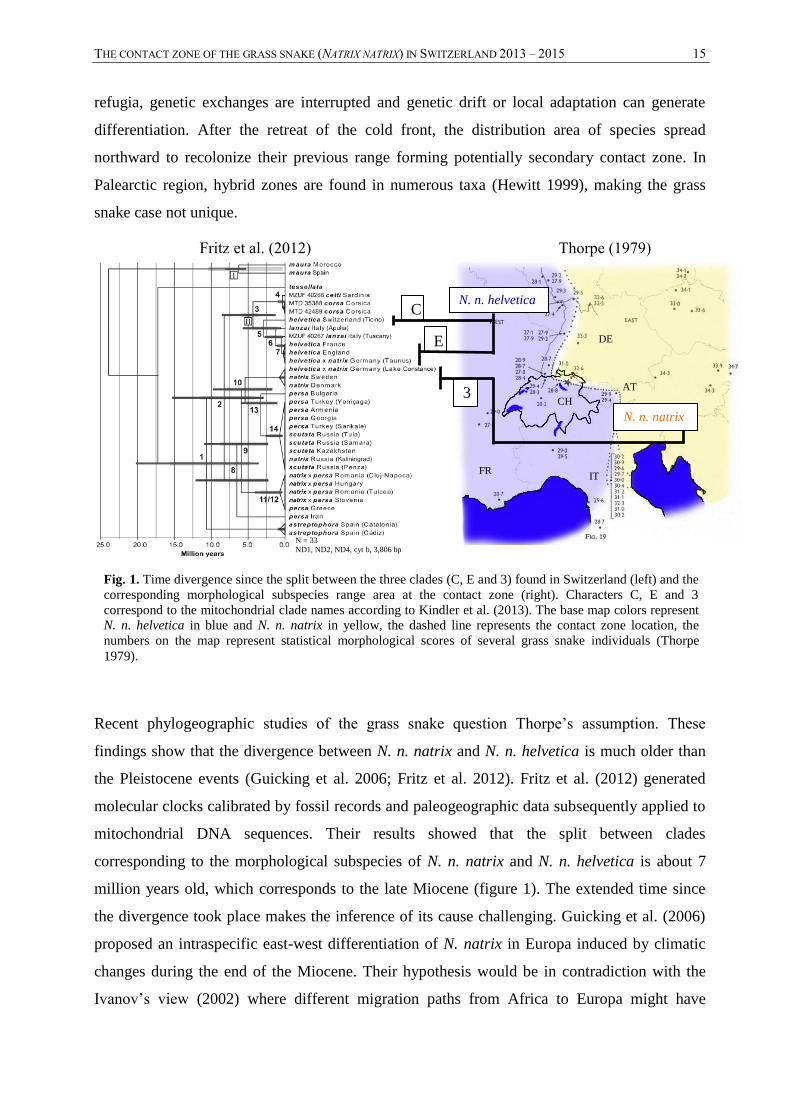
Recent phylogeographic studies of the grass snake question Thorpe’s assumption. These
findings show that the divergence between N. n. natrix and N. n. helvetica is much older than
the Pleistocene events (Guicking et al. 2006; Fritz et al. 2012). Fritz et al. (2012) generated
molecular clocks calibrated by fossil records and paleogeographic data subsequently applied to
mitochondrial DNA sequences. Their results showed that the split between clades
corresponding to the morphological subspecies of N. n. natrix and N. n. helvetica is about 7
million years old, which corresponds to the late Miocene (figure 1). The extended time since
the divergence took place makes the inference of its cause challenging. Guicking et al. (2006)
proposed an intraspecific east-west differentiation of N. natrix in Europa induced by climatic
changes during the end of the Miocene. Their hypothesis would be in contradiction with the
Ivanov’s view (2002) where different migration paths from Africa to Europa might have
Fritz et al. (2012)
N. n. helvetica
N. n. natrix
Thorpe (1979)
E
C
3 CH
FR
AT
DE
IT
Fig. 1. Time divergence since the split between the three clades (C, E and 3) found in Switzerland (left) and the
corresponding morphological subspecies range area at the contact zone (right). Characters C, E and 3
correspond to the mitochondrial clade names according to Kindler et al. (2013). The base map colors represent
N. n. helvetica in blue and N. n. natrix in yellow, the dashed line represents the contact zone location, the
numbers on the map represent statistical morphological scores of several grass snake individuals (Thorpe
1979).
N = 33
ND1, ND2, ND4, cyt b, 3,806 bp

THE CONTACT ZONE OF THE GRASS SNAKE (NATRIX NATRIX) IN SWITZERLAND 2013 – 2015 16
induced the east-west differentiation. While Guicking et al. (2006) refute Thorpe’s view on the
role of the Pleistocene period in the differentiation of the grass snake, the events 2.4 million
years ago were not without effect as they induced the current distribution of the clades in
Europe. Additionally, the Pleistocene events induced differentiation of several terminal recent
clades (Fritz et al. 2012, Kindler et al. 2013). Based on the current distributions of
mitochondrial clades, Kindler et al. (2013) located the glacial refugia for the last glaciation of
clades related to N. n. helvetica in South France (clade E) and in the Peninsula of Italy (clade C
and other not present in Switzerland) and the refuges of N. n. natrix in the Balkan Peninsula
(clade 3 and other not occurring in Switzerland). However, Kindler et al. (2013) sampled only
9 individuals from Switzerland and were not in position to infer the situation at the contact
zone, what the present study will attempt to clarify.
1.5. THE RED LISTS
The International Union for Conservation of Nature (IUCN) has compiled lists of endangered
species since the 1950s (see Mace et al. 2008 for more historical information). The main
objective of this compilation was to identify the species with the higher risk of extinction in the
world and to make this information available to the scientific and political world as well as to
the public in general. Initially, the IUCN evaluated only the mammals and the birds, and the
threat criteria were widely subjective and controversial. In the seventies, the number of taxa
recognized increased to include all known animals, plants and fungi. Moreover, the criteria
became more and more objective and based on quantitative components. Thus, the IUCN Red
List has become the most complete source of information in the world on the overall
conservation status of species (IUCN 2012).
Currently, the IUCN Red List includes 9 categories informing about the level of threat of taxa:
the categories Not Evaluated (NE) and Data Deficient (DD) define taxa requiring more data
and investigation; they also include invasive species without conservation value. The
categories Least Concern (LC) and Near Threatened (NT) define taxa, on which immediate
conservation efforts are not needed. Three categories defined different threat levels: Vulnerable
(VU), Endangered (EN) and Critically Endangered (CR). Finally the IUCN defines 2
categories for extinct data: Extinct (EX) and Extinct in the Wild (EW). The IUCN categories
were defined based on objective and quantitative criteria offering a great credibility for the
estimation of the likelihood of extinction. Five criteria allow to define the category with
THE CONTACT ZONE OF THE GRASS SNAKE (NATRIX NATRIX) IN SWITZERLAND 2013 – 2015 17
accuracy. They are mainly based on decline of population, population size, range area, habitat
fragmentation and habitat quality. Each criterion is subdivided in several sublevels, leading to a
specific code belonging to one threat category (see below for the grass snake threat level and
code). Finally, these criteria are devised for any taxonomic unit (species and subunits of
species).
The IUCN generates Red Lists at the world level. However, numerous countries use the IUCN
categories and methods to evaluate the threat status of the species at the national level. In
Switzerland the national Red Lists are legally recognized and managed by the Federal Office
for the Environment (FOEN). They are notably important to provide source on species
identification needing conservation actions, to develop strategies in the aim to preserve the
Swiss biodiversity, to control on the Swiss conservation plan efficiency, to bring useful
awareness tool for the general public and finally to give, combined with international data, a
good estimation of the situation of biodiversity at larger scale (Monney and Meyer 2005).
Monney and Meyer (2005) used the criteria and categories of the IUCN (2001) for their
compilation of the last Red List of threatened reptiles of Switzerland. The taxonomic units used
was species, subspecies and for one species, genetic clades. For Monney and Meyer, this
choice of infra-specific level, view as “evolutionary significant unit” (sensu Crandall et al.
2000), allows refining the monitoring of the biodiversity because the biodiversity monitoring
because the threat status between taxa of the same species are sometimes very different.
In Switzerland, the grass snake is actually represented by two subspecies, Natix natrix natrix,
present in the northeast of the country, and the Natrix natrix helvetica, present in the rest of
Switzerland. They are considered as, respectively, Endangered (EN) and Vulnerable (VU). The
different criteria of both subspecies in Switzerland are resumed below:
THE CONTACT ZONE OF THE GRASS SNAKE (NATRIX NATRIX) IN SWITZERLAND 2013 – 2015 18
Summary of the threat level of the Swiss grass snake based on Monney and Meyer (2005)
Natrix natrix natrix; EN; A2c, B2a, B2b (iii,iv)
• A. Reduction in population size, 2. Population size reduction of >50% over the last 10 years
c. A decline in area of occupancy, extent of occurrence and/or quality of habitat
• B. Geographic range, 2. Area of occupancy estimated to be less than 500 km2
a. Severely fragmented or known to exist at no more than five locations
b. Continuing decline, observed, inferred or projected, in any of the following: iii) area,
extent and/or quality of habitat; iv) number of locations or subpopulations
Natrix natrix helvetica; VU; A2c, B2a, B2b (iii, iv)
• A. Reduction in population size, 2. Population size reduction of >30% over the last 10 years
c. A decline in area of occupancy, extent of occurrence and/or quality of habitat
• B. Geographic range, 2. Area of occupancy estimated to be less than 2000 km2
a. Severely fragmented or known to exist at no more than five locations
b. Continuing decline, observed, inferred or projected, in any of the following: iii) area,
extent and/or quality of habitat; iv) number of locations or subpopulations
The reasons for these threat levels in both subspecies are firstly, a widespread and strong
decline of population effectifs and secondly a highly fragmentation of their habitat. The cause
of this decline is mainly attributed to the loss in amphibian habitats (Meister et al. 2012), which
are widely shared with the grass snake and contribute to their primary source of food.
Additionally, N. n. natrix was considered EN because its distribution area is very limited in the
country. At the World level, the grass snake was categorized in 2009 as least concern, without
distinction for the different subspecies (IUCN 2014,
http://www.iucnredlist.org/details/14368/1).
1.6. GENETIC MARKERS AND MORPHOLOGY
Genetic markers: mtDNA
Mitochondrial DNA (mtDNA) is a circular double-stranded molecule of DNA presents in the
mitochondrion (organelle responsible, mainly, to the cellular respiration) and constitutes a
genome independent from the nuclear DNA. Organisation of the mtDNA genome in snakes
includes 30 protein-coding genes, 22 tRNA genes, 2 rRNA genes and 2 control regions (Dong
and Kumazawa 2005). The mutation rate of mtDNA protein-coding genes is relatively high
compare to the nuclear protein-coding genes (Bromham 2002); hence, mtDNA presents
potentially a better choice to study speciation (Waugh 2007). However, it is important to note
that mutation rates do not follow strict rules between taxa and genes. For instance, variability
THE CONTACT ZONE OF THE GRASS SNAKE (NATRIX NATRIX) IN SWITZERLAND 2013 – 2015 19
exists between poikilotherms and endotherms, probably due to the variation in metabolism
levels (see Bromham 2002). The variability between genes can be illustrated by the control
region of the mtDNA, which tends to evolve faster than protein-coding genes in mammals and
birds, but the opposite pattern is observed in reptiles (Brehm et al. 2002). The mitochondrial
genome has the property to be strictly maternal inherited; therefore, recombination is very rare
and occurs only in specific isolated taxa (Krishnamurthy and Francis 2012). As the mutation
rate is relatively constant over time within taxa and between closely related species (Bromham
2002), it allows to estimate time divergence between different lineages by “molecular-clock”
(Galtier et al. 2009). The lake of recombination and the constant mutation rate makes mtDNA
an ideal choice to study phylogeny of the species and lineages. Mitochondrial DNA provides
also a powerful tool in phylogeographic studies when the different haplotypes are analysed in a
geographical dimension combined with paleogeographic data (continental drifting, ice ages, sea
levels, etc.). It gives solid basis to understand the history of molecular lineages and to delineate
taxa (representing potentially distinct evolutionary lineages). However, mtDNA sequences
used alone are not sufficient to infer strong taxonomy. In a theoretical case where two mtDNA
lineages never occur in the same area (in allopatric or parapatric patterns), mtDNA cannot
prove a total genetic integrity. Indeed, if females are sedentary, the dispersal power of mtDNA
genome will be very low showing reciprocal monophyly between putative taxa (de Queiroz
2007). Additionally, even if gene flow appears very low in mtDNA, it is possible that males
migrate and homogenize the nuclear genome.
Genetic markers: microsatellites
Complementary information provided by nuclear markers seems essential to validate
taxonomic value of mtDNA lineages from a genetic point of view. A great variety of nuclear
markers exist and their properties vary in their cost and time of development, in their level of
polymorphism or in their inheritance system (i.e. if heterozygotes can be identified). Finally,
the amount of animal tissue required for the analyses also depends on which markers are used.
This is not without importance when non-invasive methods of research are chosen for
conservation purposes. The nuclear marker “microsatellite” present the advantages to be non-
invasive, co-dominant and very polymorphic, but the development is relatively time consuming
and costly.
Microsatellites are tandem repetitive units of generally 2 to 5 base pairs (Jehle and Arntzen
2002). They are generally highly variable in length (i.e. in tandem repetitions) with high rate of
mutation and are inherited from both parents (present in the nuclear DNA). When taken at
THE CONTACT ZONE OF THE GRASS SNAKE (NATRIX NATRIX) IN SWITZERLAND 2013 – 2015 20
multiple loci, microsatellites are more adapted tools than mtDNA to study the structure of the
population. They allow to estimate genetic diversity of populations, recent demographic events
on populations or connectivity between populations providing important source of information
for endangered species (Lougheed et al. 2000). For taxonomic purposes, Mallet (2006)
emphasized the use of microsatellites that, when combined with algorithms, are able to infer
genetic clusters in hybrid zone of polytypic species. For Mallet, if subspecies freely intergrade
at the contact zone and form one cluster, the infraspecific taxonomic rank has to stay
unchanged, otherwise elevation to full species could be considered.
Morphology and comparison with genetic
Genetic and morphology are not in competition or exclusive. Instead, they serve the same goal
with different approaches (see Dayrat 2005). Dayrat (2005) stressed the need to conserve
morphological analyses in taxonomic evaluations in integration with genetic. Additionally,
Dayrat (2005) said, “… where it is shown that morphological features provide faster, more
reliable identifications [than genetic features], there is no reason to discard them” and this is
particularly true due to the fact that molecular analyses are time-consuming and costly.
Actually no studies are focused on the concordance between morphology and genetic of the
grass snake. In a first approach, Kindler et al. (2013) found clear overlapping between
morphological subspecies and mtDNA haploclades in their distribution areas suggesting bad
taxonomy within the polytypic species Natrix natrix. Such discordances are not exceptional.
For instance, several divergent mtDNA lineages with different phylogeographic patterns can
present similar morphological features only due to a shared selective pressure (e.g. on the
colour pattern directly associated with the thermoregulation of the rat snake, Burbrink et al.
2000). The findings of Burbrink et al. (2000) on the rat snake (formerly Elaphe obsolata, now
divided in four species, see Pyron and Burbrink 2009) showed that taxonomy based on few
morphological characters is unable to ensure evolutionary history of taxa. It seems clear that
the more different approaches are combined, the more taxonomic conclusions will be strong
and stable over time (Padial et al. 2010).
The intense morphological study of Thorpe (1979) showed that phenotypic differences (in
internal and external morphological characters) are strong, at least between the two forms
meeting and hybridizing in middle Europe (and for two island forms in Corsica and Sardinia).
These results are consistent with the Kindler et al.’s findings (2013) where two mtDNA basal
clades divide Europe in east and west (with an additional basal clade found in Iberian Peninsula
and north Africa), providing evidences that this contact zone occurs between deeply
THE CONTACT ZONE OF THE GRASS SNAKE (NATRIX NATRIX) IN SWITZERLAND 2013 – 2015 21
differentiated mtDNA lineages. However, the latter study was unable to clearly highlight
concordance or discordance between morphology and genetic due to the large-scale resolution.
1.7. AIMS OF THE STUDY
Taxonomy
The geographical grass snake varieties would belong to the “Ugly” subspecies (see Subspecies
concept section), because any morphological pattern seems to concur to consensually describe
these taxa. This is why there are many divergent opinions regarding the number of subspecies
within this species and about their ranges. For instance, Kabisch (1999) recognised 14
subspecies and Thorpe (1979) recognised only 4. The molecular phylogeny of this species and
its subspecies was unknown until recently (Guicking et al. 2006, Fritz et al. 2012, Kindler et al.
2013). Consequently, the debate over the number of grass snake subspecies is probably
evolving toward a new solution since Kindler et al. (2013) found discordances between
morphological subspecies and mitochondrial clades in their distribution. Thus a taxonomic
revision of Natrix natrix ssp. inspecting molecular and morphology approaches is being in
progress.
The subspecies concept received numerous critics (e.g. Burbrink et al. 2000), but presents also
potential advantages in conservation (Zink 2004). In summary, the taxonomic revaluation of
the grass snake subspecies is especially relevant to avoid setting up actions costly in time and
money for entities, which do not represent real evolutionary, taxonomic and/or conservation
value. Thus, the present study will attempt to bring new knowledge allowing to validate or not
the subspecies status of N. n. natrix and N. n. helvetica. Moreover, in the case where both
entities are valid distinct taxa (whatever their taxonomic status), I will attempt to redefine the
location of the contact zone, in order to be able to calculate with accuracy their respective
range area in Switzerland. Such information will be required for the next Red List of threatened
reptiles of Switzerland.
To achieve this taxonomic evaluation, an integrative approach was used in the sense that
several taxonomic tools are used. Different scenarios are possible between N. n. natrix and N.
n. helvetica:
- Strong evidence for separate species: congruence with several taxonomic characters and
evidence for reproductive isolation (ESC: Wiley 1978; Integrative taxonomy: de

THE CONTACT ZONE OF THE GRASS SNAKE (NATRIX NATRIX) IN SWITZERLAND 2013 – 2015 22
Queiroz 2007, Padial et al. 2010; Meiri & Mace 2007, Frankham et al. 2012) or hybrid
unfitness (DFSC: Hausdorf 2011).
- Evidence for separate species without high level of consensus: congruence with at least
two independent taxonomic characters and without requiring evidence for reproductive
isolation (DeSalle et al. 2005).
- No taxonomic change and the subspecies status are validated: evidence for
differentiation in one taxonomic character (Integration by congruence: Miralles et al.
2011, Hawlitschek et al. 2012). It shows a taxonomic and a conservation value (e.g.
providing different biological variability and richness), without strong evidence for
evolutionary differentiation (ESC: Wiley 1978; Integrative taxonomy: de Queiroz 2007,
Padial et al. 2010).
- Taxonomic changes with the non-recognition (abandonment) of the subspecies status:
no evidence for differentiation in any taxonomic characters (in the case of inconsistent
results compared to the previous morphological studies and without conclusive results
provided by the genetic).
The two taxa were identified by morphological differences and coincide probably with two
different mitochondrial clades (see the section 1.3). For some authors as DeSalle (2005) this
could be enough to class them as separate species, however in this study the contact zone is
analysed at fine scale to detect supplementary taxonomic information as reproductive isolation
and hybrids unfitness (regarding the level of mtDNA introgression and the level of nuclear
DNA admixture between taxa).
Analysis tools
In this study, two mitochondrial genes (Cyt b and ND4 + tRNAs) are used to explore the
diversity and the repartition of the mtDNA haplotypes present in Switzerland. In order to
observe the nature of the gene flow between different haploclades and/or morphological
entities, 14 microsatellites previously developed and detailed in the literature were used.
Finally, concordance between DNA markers and morphology was studied. In addition to the
taxonomic question, the morphological analyses were used to find relevant criteria allowing to
discriminate efficiently these subspecies. Univariate analyses attempted to identify diagnosable
criteria and multivariate analyses combined several criteria increasing the power of
THE CONTACT ZONE OF THE GRASS SNAKE (NATRIX NATRIX) IN SWITZERLAND 2013 – 2015 23
discrimination. Additionally, the method named “landmarks-based geometric morphometric”,
that analyses numerical pictures of the head, was also used. The aim of this latter method is to
detect diagnosable pattern in scalation or general changes in shape.
Aims
The general aim of this study is to update the knowledge of the contact zone between N. n.
natrix and N. n. helvetica, using modern tools. This study serves to locate with accuracy the
contact zone based on genetic data. The level of introgression between the two subspecies is
evaluated. When two genetic entities were observed, they were analysed to detect
morphological differences (potentially diagnostic). Genetic data will serve to calculate the
surface of occupation of both subspecies for the next Red List. Finally, this study revaluates
and discussed the taxonomic status of the two subspecies.

THE CONTACT ZONE OF THE GRASS SNAKE (NATRIX NATRIX) IN SWITZERLAND 2013 – 2015 24
Part two
MATERIALS AND METHODS

THE CONTACT ZONE OF THE GRASS SNAKE (NATRIX NATRIX) IN SWITZERLAND 2013 – 2015 25
2. MATERIAL AND METHODS
2.1. STUDY AREA AND ORIGIN OF THE SAMPLES
A total of 203 samples were collected from 66 municipalities located on an area covering
heterogeneously the territory of Switzerland. One hundred and fifty-six samples were collected
during this study between July and September 2013 and April and June 2014. The remaining
47 samples came from DNA collection of the Institut für Natur-, Landschafts- und
Umweltschutz (NLU) of UNIBAS (n = 17), the Natural History Museums of Bern (n = 4),
Basel (n = 2) and Chur (n = 2), or random occurrences (skins and road kill; n = 22). One
hundred additional animals from the natural history museums of Basel (n = 12), Bern (n = 12),
Chur (n = 20), Geneva (n = 48) and Zurich (n = 8) were analysed for morphology only
(resumed in table 1).
Table 1. Summary of the animals collected and analysed in the study. The category
“Other” take into account NLU DNA collection and random occurrences.
Field Museums Other Total
Morphology 145 (> 30 cm) 100 - 245
DNA 156 8 39 203
The sampling was focused on the assumed area of the contact zone of N. n. natrix and N. n.
helvetica (according to Thorpe 1979), comprising the cantons of Aargau, Glarus, Grisons,
Lucerne, Schaffhausen, Schwytz, St. Gallen, Thurgau and Zurich. The areas for the collection
of samples were selected for their well-preserved amphibian habitat (amphibians are the
primary diet of the grass snakes) and on the observations of Natrix natrix collected by the
karch-CSCF (Centre de Coordination pour la Protection des Amphibiens et Reptiles de Suisse
& Centre Suisse de Cartographie de la Faune). An effort was made during the capture of the
samples to limit disturbing the biotope and especially the impact on the flora and the bird nests.
A picture of the first twenty ventral scales was taken in order to avoid sampling twice the same
animal. The samples coming from a skin were not considered in the analyses if the
microsatellite analysis indicated that the same individual was sampled earlier. The animals
were captured by hand and placed in a paper bag before measurements. The different
measurements and manipulations lasted up to 45 minutes per animals. Two to four ventral
scales were collected with sterile scalpels and stored in 70% alcohol. One swab per snake was
used to collect sample of saliva, then dried and stored at -20°C. The animals were released
immediately after the end of the measurements at the specific location of the capture (marked
with GPS).

THE CONTACT ZONE OF THE GRASS SNAKE (NATRIX NATRIX) IN SWITZERLAND 2013 – 2015 26
2.2. LABORATORY PROCEDURES
2.2.1. DNA purification
Total genomic DNA was extracted from the saliva (swabs), scales, skins or, in the some case of
animals in museum and road kill, from small tail tips. The purification of the total DNA of each
individual was performed followed the protocol “Purification of total DNA from Animal
Tissues (Spin-Column Protocol)” (DNeasy Blood & Tissue Kit, Qiagen). The scales stored in
70% ethanol were previously placed in water during 24 hours to remove the ethanol from the
tissue. When DNA was extracted from saliva, followed the same protocol as for normal animal
tissue, but the wad of cotton of the swab was removed after the bind step. A representative
sample of DNA template was analysed with the NanoDrop (ThermoFisher scientific) to
quantify the amount of DNA after the first extraction.
2.2.2. Mitochondrial DNA amplification and sequencing
In order to assign the samples to a genetic clade, two mitochondrial genes were used, including
the cytochrome b gene (Cyt b) and the NADH dehydrogenase subunit 4 gene with the adjacent
region coding for tRNA-His, tRNA-Ser and tRNA-Leu (ND4 + tRNAs). Both genes were
previously used to study the phylogeny of the grass snake and sibling species (Guicking et al.
2006; Fritz et al. 2012; Kindler et al. 2013).
The PCR were performed with a Mastercycler Pro (eppendorf) using the Taq PCR Core Kit
(Quiagen) in 25 µl reaction volumes with 3 µl DNA template, 0.5-1 U Taq polymerase, 1x
buffer with MgCl2, 2 mM MgCl2, 0.2 mM dNTP each, 2mg/ml Q sol and 0.5 µM for primers
(cycles and temperatures conditions for the primers are available in the Annexes, table A1).
Sequencing of 20 µl of PCR product was performed by Macrogen Europe with a ABI 3730XLs
sequencer (Applied Biosystems). Genes were sequenced from both sides using the primers
detailed in the Annexes (table A1). Sequences were aligned and inspected using CodonCode
Aligner 4.03. (CODONCODE CORPORATION) guided by four GenBank sequences (ND4 +
tRNAs : HF679634, HF679623; cyt b : AY487748, AY866544). Kindler and collaborators
(2013) found no significant changes in phylogenetic analyses treating both genes separated or
not. Then, Cyt b and ND4 + tRNAs sequences from each individual were concatenated in one
single record.

THE CONTACT ZONE OF THE GRASS SNAKE (NATRIX NATRIX) IN SWITZERLAND 2013 – 2015 27
2.2.3. Microsatellites amplification and sequencing
To infer the number of genetic clusters and the level of admixture between them, 13 out of 14
microsatellites (listed in the Annexes, table A2) were used in the analyses. Indeed, Nsµ3
presented problems either for amplification or by the presence of null alleles and was removed
from the analyses in the early stages of the laboratory work. PCR amplifications were
performed with a Mastercycler Pro (eppendorf) in a final volume of 10 µl containing 2 µl of
template DNA, 5 µl Type-it Microsatellite PCR Kit (Qiagen) with specific volumes and
concentrations for each primer (detailed in the Annexes, table A2), finally ddH2O was added to
obtain a total of 10 µl. Forward primers were marked with a fluorescent dye (from Applied
Biosystems) specified in the Annexes (table A2). The thermocycling conditions used for
amplifications were: initial incubation at 95°C for 5 minutes, followed by 32 cycles of
denaturing at 95°C for 30 seconds, annealing at 54°C (for multiplex-PCR 1) or 55°C (for
multiplex-PCR 2) for 90 seconds and extension at 72°C for 30 seconds, finished by a final
extension step at 60°C for 30 minutes. PCR products of multiplex-PCR 1 and multiplex-PCR 2
mixed with Nsµ2 were analysed with an AB3130xl Genetic Analyzer (Applied Biosystems) in
the Zoological Institute of the University of Basel. Peaks were visualized using Peak Scanner
Software v1.0 (Applied Biosystems).
2.3. GENETIC DATA ANALYSES
2.3.1. Mitochondrial DNA
The mtDNA sequences were compared with BLAST allowing the assignment of the two
haploclades present in northeast Switzerland: clade E corresponding to the subspecies N. n.
helvetica or clade 3 corresponding to N. n. natrix, according to Kindler et al. (2013). The
individuals represented by their associated clade were mapped to observe the distribution
pattern. The genealogical relationship between and within clades was examined using TCS
v1.21 (Clement et al. 2000) with a connection limit of 95%. This software built genealogical
network using statistical parsimony.
THE CONTACT ZONE OF THE GRASS SNAKE (NATRIX NATRIX) IN SWITZERLAND 2013 – 2015 28
2.3.2. Microsatellites
Linkage disequilibrium
Linkage disequilibrium was inspected using FSTAT v 2.9.3 (Goudet 1995, 2001) to test if
microsatellite loci are independent from each other. Linkage disequilibrium was tested in each
mitochondrial clade.
Population structure
A Bayesian clustering method based on Markov chain Monte Carlo implemented in
STRUCTURE v 2.3.4 (Pritchard et al. 2000) was used to assess the number of genetic
populations without prior clustering information. The algorithms allow finding the most likely
number of populations (K) approaching Hardy-Weinberg equilibrium. Moreover, they estimate
the level of admixture between the inferred populations. Twenty pseudo-replicates were run for
200’000 iterations after a period of 100’000 iterations as burn-in. The number (K) of
genetically homogeneous groups (clusters) was tested between 1 and 20. To detect the higher
level of genetic organization, the method of ∆K was applied, according to Evanno et al. (2005).
Indeed, the maximum value of the likelihood L(K) returned by STRUCTURE was not directly
used to detect the number of clusters, because this would only indicate the number of local
populations sufficiently distant. A study in population genetics showed that populations of N.
n. helvetica separated from 30 km could already induce genetic clusters with STRUCTURE
(Meister et al. 2012). In the present study, the research area could be subdivided in numerous
populations, and the aim of the main project is to determine if gene flow occurs between the
two subspecies. Consequently, the first level of structuration only is relevant in this study and
the ∆K method more appropriate.
Finally, to test the robustness of the results each locus was tested separately in STRUCTURE
with the same settings used for the full dataset, except for the number of pseudo-replicates (n =
15). The results returned by STRUCTURE were compiled with STRUCTURE HARVESTER (Earl
2012) to interpret the most likely K with the ∆K method (where the modal value of ∆K
indicates the most likely K value).
The relationship between the genetic and geographical location at the contact zone was inferred
with GENELAND (Guillot et al. 2005). The R package Geneland v4.0.5, also based on Bayesian
clustering, uses genetic data combined with geographical information. This package generates
map by assigning to any pixel a posterior probability to belong to different genetic cluster.
THE CONTACT ZONE OF THE GRASS SNAKE (NATRIX NATRIX) IN SWITZERLAND 2013 – 2015 29
Such map allows to detect genetic discontinuity between population and in some case recent
migrants can be detected. Ten pseudo-replicates of K between 1 and 10 were run with 50’000
iterations and a thinning of 100. As in STRUCTURE analyses, 194 individuals and 13
microsatellites were used.
Population-based analysis
The fixation index (FST) was used to analyse the isolation by distance and to estimate genetic
differentiation between pairs of populations within and between subspecies. Isolation by
distance was analysed with the method of Rousset (1997). This method uses the regression of
FST/(1-FST) estimates for pairs of populations on the logarithm of geographical distance. No
population was sampled exhaustively (i.e. more than 20 individuals in the same location), due
to the difficulty to found these animals and the will to diversify the sampling locations.
However 10 small locations including between 5 and 10 individuals were selected (Annexes,
table A6). The grouping criteria were: i) individuals close to maximum 4 km, ii) populations
showing concordance between mtDNA and nDNA and iii) population without important
nuclear admixture. Pairwise comparisons between locations of both subspecies led to three
relationship classes: natrix x natrix (n = 10), helvetica x helvetica (n = 10) and natrix x
helvetica (n = 25). The aim of this operation was to see if inter-subspecific (natrix x helvetica)
pairwise comparisons were different that the intra-subspecific pairwise comparisons (natrix x
natrix and helvetica x helvetica) as expected in case of a reduced gene flow between
subspecies. Pairwise FST and distance matrix were calculated with GenAlEx 6.5 (Peakall and
Smouse 2006, 2012). Correlation between FST/(1-FST) and logarithm of distance was calculated
using Mantel correlation coefficient rm. Mantel tests were performed using FSTAT v 2.9.3
(Goudet 1995, 2001) with 10’000 randomizations. Comparisons between FST/(1-FST) means in
the different classes were performed with multiple comparisons using Games-Howell test
(Games and Howell 1976). This test was used because homoscedasticity was not met and
geographical distance did not significantly act as covariance.
Relatedness between individuals
FST analyses can lack of statistical power when a limited number of individuals by population
are analysed. Consequently a relatively similar analysis was conducted focused on the
THE CONTACT ZONE OF THE GRASS SNAKE (NATRIX NATRIX) IN SWITZERLAND 2013 – 2015 30
individuals. The aim of this analysis was to observe isolation by distance and genetic
differentiation between subspecies at individual level. Pairwise relatedness between individuals
of both subspecies (n = 194) was calculated using the Lynch & Ritland’s (1999) estimator as
implemented in GenAlEx 6.5 (Peakall and Smouse 2006, 2012). This estimator returns values
between -0.5 and 0.5, where pairs of individuals closely related tends to approach 0.5. Pairwise
comparisons between all individuals of both subspecies led to three relationship classes: natrix
x natrix (n = 5050), helvetica x helvetica (n = 4278) and natrix x helvetica (n = 9393). Multiple
comparisons with ANCOVA (With Tukey HSD test) were performed using the R package HH
v1.4 (Heiberger and Holland 2004) to compare relatedness between the three classes with
geographical distance as covariance. The normality was assumed, despite a slight positive
skewness in the distribution of the residuals. Bartlett test of homogeneity of variances did not
allow to accept null hypothesis that homoscedasticity was assumed (N = 18’721, K-squared =
1468.71, df = 2, p-value < 0.0001). Thus, interpretations of the ANCOVA have to be
considered with prudence. Correlations between relatedness estimations and geographical
distance were calculated using the same method as for the population-based analysis (Mantel
test).
2.4. MORPHOLOGICAL DATA ACQUISITION
2.4.1. Criteria selection
The morphological criteria measured were selected in accordance with the results of Thorpe’s
study (1979); only non-intrusive morphological criteria, showing strong tendencies for
differences, were selected. A total of 20 variables (listed here below and detailed in the
Annexes, table A3) were measured. This concerns 15 continuous quantitative variables: snout-
vent length (SVL), tail length (TL), head width (HW), head length (HL), body weight (WGT),
lateral blotches surface (LB.S), lateral blotches length (LB.L), lateral blotches width (LB.W),
nuchal marking size (NM.S), nuchal marking length (NM.L), degree of upper-curvature of the
nuchal markings (UC.NM), degree of lower-curvature of the nuchal markings (LC.NM),
degree of separation of the parietal scales and nuchal markings (DS.P.NM), degree of
separation of the pair of lunar markings (DS.LM), and the relative position of the reduction
from 19 to 17 dorsal scale rows (X.RNS). There are 4 quantitative discrete variables: number
of ventral scale (V), number of paired subcaudal scales (SC), number of post-temporal scale
(PT) and number of gular scales (G). Finally, the contact between the temporal and the lower
THE CONTACT ZONE OF THE GRASS SNAKE (NATRIX NATRIX) IN SWITZERLAND 2013 – 2015 31
post-ocular scale (C.T.PO) was the single quantitative variable measured. The terminology is
based on Thorpe (1975) and on Peters (1985).
Juveniles smaller than 30 cm were removed from all morphological analyses, because the
allometric discrepancies generated by the age and size were too important, even when applying
allometric correction (Thorpe 1979). Allometry occurs for characters without linear growth.
For Natrix natrix characters with high level of allometry contained head measures and body
weight (Gregory 2004), the tail length was not under this restriction according to the study’s
author. In univariate analyses, all criteria without high level of allometry were used to analyse
animals larger than 30 cm. The threshold for head measurements and body mass was taken at
50 cm. Only individuals larger than 50 cm were considered for multivariate analyses.
Individuals from museum were no taken into account for the body mass as they were gorged
with alcohol or formalin. Sex was determined based on the size (diameter) of the tail after the
cloaca that remains constant in males but reduces in diameter in females.
2.4.2. Morphological measurements
Measurement tools were an electronic scale (body mass), a meter stick or a rigid string (SVL
and tail length), a digital caliper (head measures). Other measurements were estimated through
visual observations. Visual observation can potentially induce inaccuracies, however, errors in
observations are expected to be constant throughout the collections of data as only one
researcher collected all the visual observations.
To test the reliability of the measurements, 49 individuals chosen randomly were measured a
second time for the lateral blotches length (based on numerical pictures). The new
measurements were subtracted to the old measurements and the differences were tested with a
Student’s t-test to see if the error significantly differs from 0. The results of the test (one-
sample t 48 = -1.4078, p-value = 0.1656) show a relative consistency in the measurements.
2.4.3. Geometric morphometrics
Based on head photographs of the grass snake, the aim of these analyses is to detect changes in
shape or potentially diagnostic criteria between N. n. natrix and N. n. helvetica. As for the other
morphological analyses, individuals were assigned to a subspecies when the proportion of
ancestry returned by STRUCTURE was > 0.8. Only the individuals longer than 50 cm were
selected to limit allometric bias.
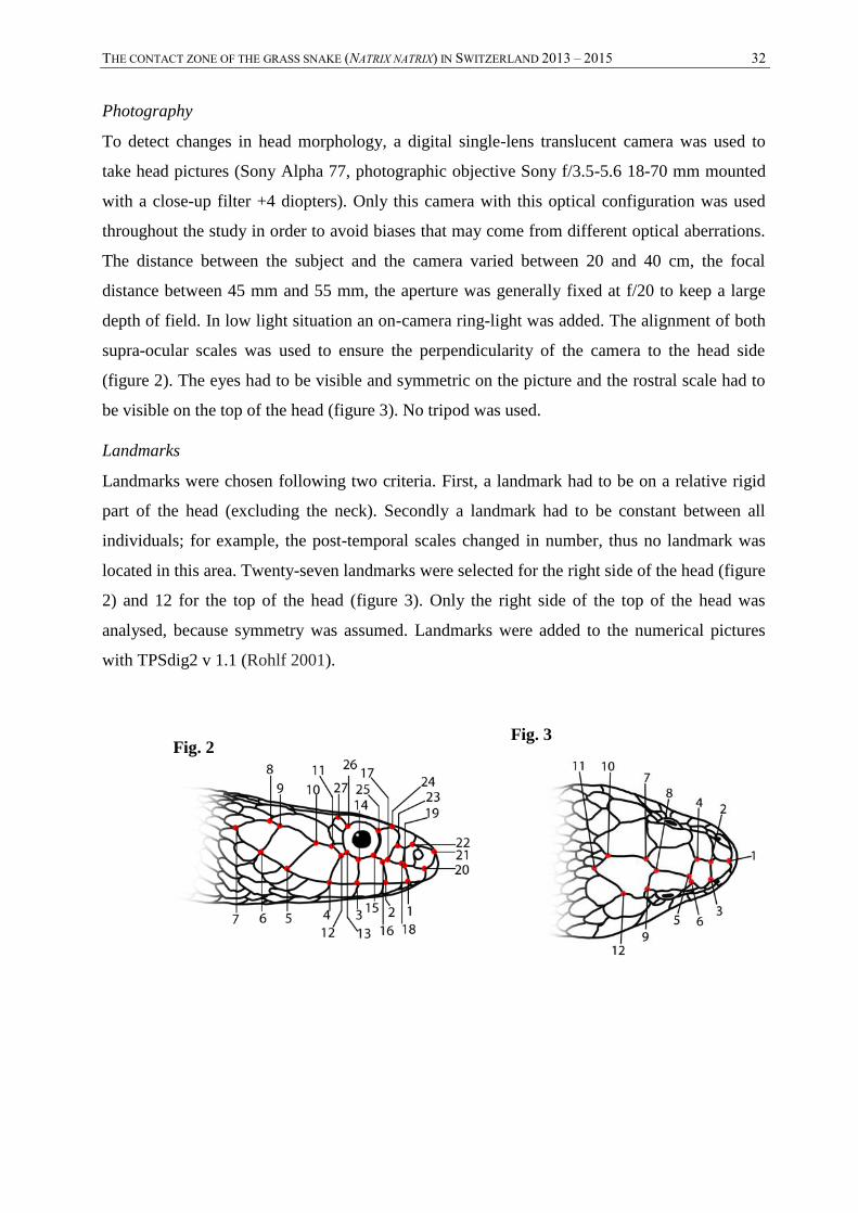
THE CONTACT ZONE OF THE GRASS SNAKE (NATRIX NATRIX) IN SWITZERLAND 2013 – 2015 32
Photography
To detect changes in head morphology, a digital single-lens translucent camera was used to
take head pictures (Sony Alpha 77, photographic objective Sony f/3.5-5.6 18-70 mm mounted
with a close-up filter +4 diopters). Only this camera with this optical configuration was used
throughout the study in order to avoid biases that may come from different optical aberrations.
The distance between the subject and the camera varied between 20 and 40 cm, the focal
distance between 45 mm and 55 mm, the aperture was generally fixed at f/20 to keep a large
depth of field. In low light situation an on-camera ring-light was added. The alignment of both
supra-ocular scales was used to ensure the perpendicularity of the camera to the head side
(figure 2). The eyes had to be visible and symmetric on the picture and the rostral scale had to
be visible on the top of the head (figure 3). No tripod was used.
Landmarks
Landmarks were chosen following two criteria. First, a landmark had to be on a relative rigid
part of the head (excluding the neck). Secondly a landmark had to be constant between all
individuals; for example, the post-temporal scales changed in number, thus no landmark was
located in this area. Twenty-seven landmarks were selected for the right side of the head (figure
2) and 12 for the top of the head (figure 3). Only the right side of the top of the head was
analysed, because symmetry was assumed. Landmarks were added to the numerical pictures
with TPSdig2 v 1.1 (Rohlf 2001).
Fig. 2 Fig. 3
THE CONTACT ZONE OF THE GRASS SNAKE (NATRIX NATRIX) IN SWITZERLAND 2013 – 2015 33
2.5. MORPHOLOGICAL DATA TREATMENTS
2.5.1. Univariate analyses
Females and males were processed separately; the sexual dimorphism is known to be important
for this species (Thorpe 1989, the present study: Annexes, figure A6). Therefore, independent
variables used were sex and subspecies leading to 4 conditions. The independence of the data
was ensured by genetic results (individuals were assigned for one subspecies when proportion
of ancestry value returned by STRUCTURE was superior to 0.8). The individuals close to 10 km
of the center of the contact zone (inferred by GENELAND) without genetic data (from museum)
were excluded from the analyses. The measured characters led to 19 dependent variables (see
table A3):
- Criteria for the body proportion (n = 5): relative tail size (X.TL = TL/total body length),
relative head length (X.HL = HL/SVL), relative head width (X.HW = HW/SVL), head
shape (H.S = HW/HL) and body shape (X.WGT = weight / total body length).
- Criteria for scalation (n = 6): number of ventral scales (V), number of paired subcaudal
scales (SC), relative position of the reduction from 19 to 17 dorsal scale rows (X.RNS),
contact between the temporal and the lower post-ocular scales (C.T.PO), maximum
number of post-temporal scales (PT.MAX) and number of gular scales (G).
- Criteria for the colour pattern (n=8): lateral blotches surface (LB.S), lateral blotches
length (LB.L), lateral blotches width (LB.W), nuchal marking size (mean of both sides;
NM.S.MEAN), nuchal marking length (mean of both sides; NM.L.MEAN), degree of
separation of the parietal scales and nuchal markings (DS.P.NM), degree of separation of
the pair of lunar markings (DS.LM) and nuchal marking shape (NM.SH = [UC.NM+1] /
[LC.NM+1]). The last character combines information of the degree of upper-curvature
of the nuchal markings (UC.NM) and the degree of lower-curvature of the nuchal
markings (LC.NM). One was added to avoid division by 0.
The total length was analysed to explore the sample homogeneity. Females presented
homogeneous data (ANOVA, F1, 118 = 0.0028, p-value = 0.9581), but males between both
subspecies were significantly different (ANOVA, F1, 87 = 6.38, p-value = 0.0134), where N. n.
helvetica individuals were 7% larger. Since allometry was not controlled, results of variables
under allometric effect (head and body proportions) have to be considered with prudence.
THE CONTACT ZONE OF THE GRASS SNAKE (NATRIX NATRIX) IN SWITZERLAND 2013 – 2015 34
Parametric variables were analysed by one-way ANOVA where results were validated after
analyses of equality of variances and normality of residuals. Homogeneity of the variance
(homoscedasticity) was tested with a Bartlett test. Normality of the data were explored with
quantile-quantile plots and tested with Shapiro-Wilk normality test. When right-skewed was
detected, natural log was applied to the data and analyses were reiterated. When normality was
still not observed after the natural log application and data seemed non-parametric, the
variables were tested with a Wilcoxon test. When normality was respected but not the
homoscedasticity, a Student’s t-test with Welch approximation to the degrees of freedom was
applied. Two quantitative discrete variables were considered as qualitative variables (C.T.PO
and PT.MAX). Qualitative variables were compared with a Chi-square test. The statistical test
applied to the variables is indicated on the results table (table A4, A5). Statistical significance
was taken as P < 0.05. All statistical analyses were performed with RStudio v 0.98.1049
(RStudio 2012).
2.5.2. Multivariate analyses
Principal component analyses (PCA) were performed to explore dependent variables with the
objective to find optimal morphological characters to discriminate subspecies. The PCA were
performed with the R package stats v 3.1.3 and bivariate plots were performed with the R
package ggbiplot v 0.55. This first PCA contained all individuals (n = 231) and all continuous
variables used in univariate analyses (n = 17), thus both sexes, missing data replaced by the
mean and also individuals with nDNA admixture. Individuals with nDNA admixture
(individuals with a proportion of ancestry returned by STRUCTURE inferior to 0.8), could be
seen as “hybrids”. Missing data came mainly from museum individuals with skin colour
deterioration, melanistic pattern, faded or absent lunar markings or rare aberrations in
measurements. For the next steps, the sexes were separated due to the important sexual
dimorphism. PCA with females had 139 individuals and PCA with males had 92 individuals.
The selected variables for the next step where chosen when contribution for PC1 (axe
discriminating subspecies) was more than 5%. Then, these chosen variables were used in 2
PCAs: one PCA with “hybrids” and with missing data and the second without hybrids and
without missing data. To display the consistency between morphology, genetic and geography,
the PC1 scores of both analyses were mapped combined with microsatellite data (GENELAND
results). Finally, discriminant analyses were performed with datasets containing the chosen
variables, with and without hybrid (4 analyses). The analyses without hybrids do not take into
account the missing data; the aim was to identify the potential of discrimination in optimal
THE CONTACT ZONE OF THE GRASS SNAKE (NATRIX NATRIX) IN SWITZERLAND 2013 – 2015 35
configuration. Removing missing data is often view as ambiguous because the reason of their
presence could be a response variable. In this case, only the missing data in males about lunar
marking are susceptible to have influence on the results (it concerns 6 removed males), but the
impact is assumed negligible. Discriminant functions were performed with the R package mda
(Hastie et al. 2013). Validity of the model built by the discriminant function was tested by
repeated random sub-sampling validation. Sub-sampling validation consisting in a random
selection of 85% of the individuals to build the model, followed by a test step with the
remaining 15% individuals. A mean on 100 iterations gave the final result of the ability to
assign correctly individuals for their genetically inferred subspecies. All multivariate analyses
were performed with RStudio v 0.98.1049 (RSudio 2012).
2.5.3. Landmark-based geometric morphometric
The number of individuals selected for these analyses strongly decreased compared to the
univariate and multivariate analyses. The reason is that numerous snakes coming from the
museums present important head deformation (due to the long-term storage or physical
injuries). Thus the photographs used came principally from alive animals. Analyses on the side
of the head compared 38 females natrix with 28 females helvetica and 41 males natrix with 24
males helvetica. Analyses of the top of the head compared 39 females natrix with 31 females
helvetica and 43 males natrix with 25 males helvetica.
Statistical analyses for geometric morphometric were performed with MorphoJ v1.05f
(Klingenberg 2011). Discriminant analysis was chosen because it is an efficient statistical tool
to know if different groups can be distinguished reliably. In this case, discriminant function
was performed with a leave-one-out cross-validation, this validation built a model with all
individuals except one and then tests the model with the remaining individual. This approach is
repeated for each individual to give the ability to assign correctly individuals for their
genetically inferred subspecies. The shape changes were amplified with a factor of 3 to
improve visibility.
2.6. GEOGRAPHIC INFORMATION SYSTEM (GIS)
The geographic repartition of haplotypes, nuclear data, and morphological variability was
mapped using QGIS v 1.8 (QGIS 2012). Orthophoto of the Switzerland was provided freely by
Swisstopo.

THE CONTACT ZONE OF THE GRASS SNAKE (NATRIX NATRIX) IN SWITZERLAND 2013 – 2015 36
Part three
RESULTS
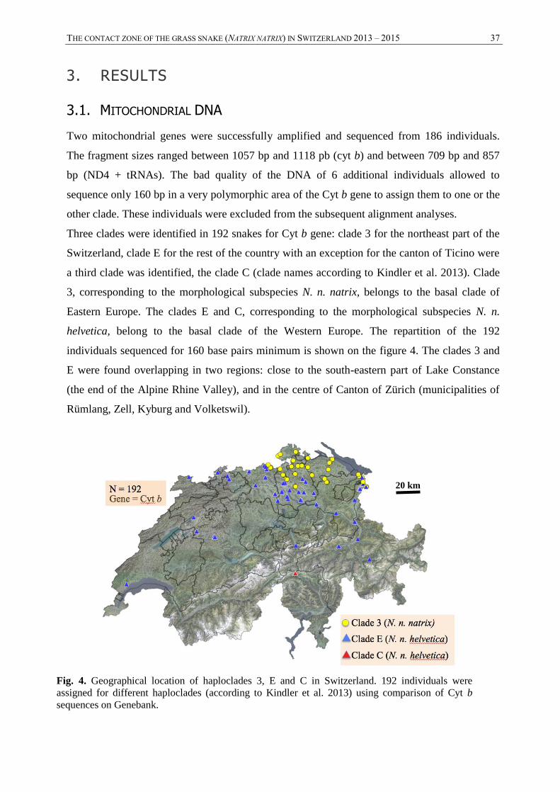
THE CONTACT ZONE OF THE GRASS SNAKE (NATRIX NATRIX) IN SWITZERLAND 2013 – 2015 37
3. RESULTS
3.1. MITOCHONDRIAL DNA
Two mitochondrial genes were successfully amplified and sequenced from 186 individuals.
The fragment sizes ranged between 1057 bp and 1118 pb (cyt b) and between 709 bp and 857
bp (ND4 + tRNAs). The bad quality of the DNA of 6 additional individuals allowed to
sequence only 160 bp in a very polymorphic area of the Cyt b gene to assign them to one or the
other clade. These individuals were excluded from the subsequent alignment analyses.
Three clades were identified in 192 snakes for Cyt b gene: clade 3 for the northeast part of the
Switzerland, clade E for the rest of the country with an exception for the canton of Ticino were
a third clade was identified, the clade C (clade names according to Kindler et al. 2013). Clade
3, corresponding to the morphological subspecies N. n. natrix, belongs to the basal clade of
Eastern Europe. The clades E and C, corresponding to the morphological subspecies N. n.
helvetica, belong to the basal clade of the Western Europe. The repartition of the 192
individuals sequenced for 160 base pairs minimum is shown on the figure 4. The clades 3 and
E were found overlapping in two regions: close to the south-eastern part of Lake Constance
(the end of the Alpine Rhine Valley), and in the centre of Canton of Zürich (municipalities of
Rümlang, Zell, Kyburg and Volketswil).
Fig. 4. Geographical location of haploclades 3, E and C in Switzerland. 192 individuals were
assigned for different haploclades (according to Kindler et al. 2013) using comparison of Cyt b
sequences on Genebank.
20 km
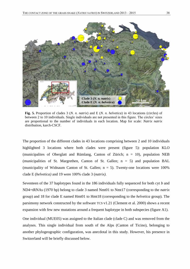
THE CONTACT ZONE OF THE GRASS SNAKE (NATRIX NATRIX) IN SWITZERLAND 2013 – 2015 38
The proportion of the different clades in 43 locations comprising between 2 and 10 individuals
highlighted 3 locations where both clades were present (figure 5): population KLO
(municipalites of Oberglatt and Rümlang, Canton of Zürich; n = 10), population NEB
(municipalities of St. Margrethen, Canton of St. Gallen; n = 5) and population BAL
(municipality of Widnaum Canton of St. Gallen; n = 5). Twenty-one locations were 100%
clade E (helvetica) and 19 were 100% clade 3 (natrix).
Seventeen of the 37 haplotypes found in the 186 individuals fully sequenced for both cyt b and
ND4+tRNAs (1970 bp) belong to clade 3 named Nmt01 to Nmt17 (corresponding to the natrix
group) and 18 for clade E named Hmt01 to Hmt18 (corresponding to the helvetica group). The
parsimony network constructed by the software TCS v1.21 (Clement et al. 2000) shows a recent
expansion with few new mutations around a frequent haplotype in both subspecies (figure A1).
One individual (MUE05) was assigned to the Italian clade (clade C) and was removed from the
analyses. This single individual from south of the Alps (Canton of Ticino), belonging to
another phylogeographic configuration, was anecdotal in this study. However, his presence in
Switzerland will be briefly discussed below.
Fig. 5. Proportion of clades 3 (N. n. natrix) and E (N. n. helvetica) in 43 locations (circles) of
between 2 to 10 individuals. Single individuals are not presented in this figure. The circles’ sizes
are proportional to the number of individuals in each location. Map for scale: Natrix natrix
distribution, karch-CSCF.
20 km Clade 3 (N. n. natrix)
Clade E (N. n. helvetica)
THE CONTACT ZONE OF THE GRASS SNAKE (NATRIX NATRIX) IN SWITZERLAND 2013 – 2015 39
3.2. MICROSATELLITES
One hundred ninety four individuals were successfully genotyped for 13 microsatellites with a
total of 0.32% of missing alleles. All loci were polymorphic: between 5 and 42 alleles were
detected with a mean ± SE of 13.5 ± 2.6. The exact number of alleles per locus is available in
the Annexes, table A2. While no linkage disequilibrium was found in clade 3, high level of
linkage disequilibrium were found in clade E between pairs of microsatellite loci: µN8new x
Natnat06, µN8new x 3TS, Natnat09 x TbuA09, Natnat05 x Hb30. However, no linkage
disequilibrium was found at any loci when introgressed individuals (see below) were removed.
Consequently, the independence between the loci is presumed. This result is in accordance with
the study of Meister et al. (2012), in which the 7 microsatellites (Natnat05, Natnat06, Natnat09,
Natnat11, µNt3, µNt7 and µNt8new) used as well in this present research presented as well no
linkage disequilibrium.
3.2.1. Population structure
The results returned by STRUCTURE and subsequently analysed with the ∆K method (Evanno et
al. 2005) indicated that 2 genetic clusters (K = 2) were the most likely options (Annexes, figure
A2). The proportion of ancestry (PoA) corresponding to the proportions of cluster membership
for all individuals are shown in figure A4 (Annexes), while the exact values are available in
table A9 (Annexes).
The mapping of the proportion of ancestry showed that one cluster corresponding to the
subspecies (N. n. helvetica) is found in the Southwest while the other cluster (N. n. natrix) is
located in the Northeast. The proportion of ancestry in the cluster helvetica was higher than 0.9
in 75 individuals, was between 0.9 and 0.8 in 13 individuals and between 0.8 and 0.5 in 13
other individuals. The proportion of ancestry of individuals belonging to the cluster natrix was
higher than 0.9 for 76 individuals, was between 0.9 and 0.8 for 7 individuals and between 0.8
and 0.5 for 10 individuals. The mapping of the proportion of ancestry gives a better
interpretation of the results, shown in figure 6.
The results of STRUCTURE and GENELAND present a strong consistency. Therefore, the number
of genetic clusters remains K=2 for GENELAND and the location of the contact zone does not
differ.
THE CONTACT ZONE OF THE GRASS SNAKE (NATRIX NATRIX) IN SWITZERLAND 2013 – 2015 40
Figure A3 (Annexes) shows the distribution of mitochondrial clades in relation to the nuclear
data. Overlapping is found in 7 locations within 10 km from the centre of the contact zone,
inferred by GENELAND (Annexes, figure A3 and A4). In 4 of these 7 locations, clade E
(helvetica) is found among populations belonging to the cluster natrix (13 individuals within 5
km of the centre of the contact zone and 2 more within 10 km) and clade 3 (natrix) was found
among the cluster helvetica in the 3 remaining locations, all within 5 km from the centre of the
contact zone.
The presence of both clusters in the same population was identified in a single population BAL
(municipality of Widnau - SG) where pure form of helvetica (BAL04, PoA for helvetica =
0.964, clade E) and presumed hybrid of natrix form (BAL01, PoA for natrix = 0.524, clade E)
were found. This latter individual is potentially a F1 hybrid; it is a male and is hypothetically
the result of mating between a local helvetica female (the population BAL being mainly
helvetica for nDNA and mtDNA) and a migrant natrix male. However, as this hypothesis is
difficult to confirm, all presumed hybrids (PoA < 0.8) are treated in a category by themselves.
When each locus was separately analysed, K = 2 was still the most likely option for all loci
excepted for Hb30 where the most likely K were 12 or 3 (the amplitude of ∆K was almost the
same for both K). The proportion of ancestry mapped for each independent locus showed still a
southwest-northeast pattern for all loci with some variability (figure A5). Only Hb30, Nsµ2 and
µNt7 tended to show a higher level of admixture.

THE CONTACT ZONE OF THE GRASS SNAKE (NATRIX NATRIX) IN SWITZERLAND 2013 – 2015 41
Base map colors: posterior
probabilities of population
membership for N. n. natrix
(GENELAND)
Proportion of Ancestry for
N. n. natrix (STRUCTURE)
Fig. 6. Population structure at the contact zone between N. n. natrix and N. n. helvetica. Circles
represent the individuals (n = 194) and colors represent their associated proportion of ancestry
returned by STRUCTURE 2.3.4 (Pritchard et al. 2000). As there are two populations, only the
proportion of ancestry for N. n. natrix is shown, proportion of ancestry for N. n. helvetica
corresponding to the remaining proportion. Base map colors represent posterior probabilities of
population membership returned by GENELAND 4.0.5 (Guillot et al. 2005).
20 km

THE CONTACT ZONE OF THE GRASS SNAKE (NATRIX NATRIX) IN SWITZERLAND 2013 – 2015 42
3.2.2. Population-based analysis
In order to evaluate the impact of the geographical distance on the genetic differentiation
between locations of both taxa, pairwise FST between each location have been calculated and
analysed. This approach involves treating separately three relationship classes: natrix x natrix,
helvetica x helvetica and natrix x helvetica locations. Pairwise FST between pairs of locations
of both subspecies in relation to the geographical distance are plotted in figure 7 according to
the method developed by Rousset (1997). Mantel test revealed no significant correlation
between FST/(1-FST) and geographical distance (Ln transformed) for pairs of helvetica x
helvetica populations (rm = 0.0889, p-value = 0.787), natrix x natrix popualtions (rm = 0.193,
p-value = 0.581) and helvetica x natrix populations (rm = 0.234, p-value = 0.264). Thus,
significant isolation by distance is not observed. Games-Howell test (summarised in table 2)
found no significant difference for FST/(1-FST) means between both intra-subspecies classes,
but significant differences between intra-subspecies classes and inter-subspecies class. Means ±
standard error in FST values without transformation were 0.092 ± 0.021 for the class helvetica x
helvetica, 0.078 ± 0.017 for the class natrix x natrix and 0.286 ± 0.048 for the class helvetica x
natrix. These results show a high genetic differentiation between natrix and helvetica
populations independently of the geographical distance.
helvetica x helvetica
natrix x natrix
helvetica x natrix
helvetica x helvetica
natrix x natrix
helvetica x natrix
Fig. 7. Isolation by distance in 10 locations of grass snake. Genetic distance (FST) as
function of geographical distance (m) using the method proposed by Rousset (1997).
Comparisons are pairwise FST between pairs of locations. Locations of both subspecies
were used (n = 5 helvetica and n = 5 natrix) with a minimum of 5 up to 10 individuals.
100 km 5 km
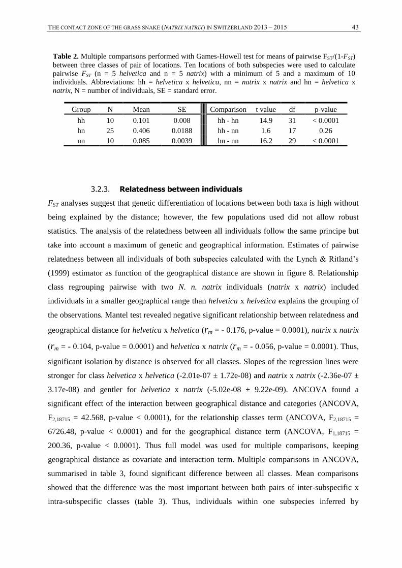
THE CONTACT ZONE OF THE GRASS SNAKE (NATRIX NATRIX) IN SWITZERLAND 2013 – 2015 43
3.2.3. Relatedness between individuals
FST analyses suggest that genetic differentiation of locations between both taxa is high without
being explained by the distance; however, the few populations used did not allow robust
statistics. The analysis of the relatedness between all individuals follow the same principe but
take into account a maximum of genetic and geographical information. Estimates of pairwise
relatedness between all individuals of both subspecies calculated with the Lynch & Ritland’s
(1999) estimator as function of the geographical distance are shown in figure 8. Relationship
class regrouping pairwise with two N. n. natrix individuals (natrix x natrix) included
individuals in a smaller geographical range than helvetica x helvetica explains the grouping of
the observations. Mantel test revealed negative significant relationship between relatedness and
geographical distance for helvetica x helvetica (rm = - 0.176, p-value = 0.0001), natrix x natrix
(rm = - 0.104, p-value = 0.0001) and helvetica x natrix (rm = - 0.056, p-value = 0.0001). Thus,
significant isolation by distance is observed for all classes. Slopes of the regression lines were
stronger for class helvetica x helvetica (-2.01e-07 ± 1.72e-08) and natrix x natrix (-2.36e-07 ±
3.17e-08) and gentler for helvetica x natrix (-5.02e-08 ± 9.22e-09). ANCOVA found a
significant effect of the interaction between geographical distance and categories (ANCOVA,
F2,18715 = 42.568, p-value < 0.0001), for the relationship classes term (ANCOVA, F2,18715 =
6726.48, p-value < 0.0001) and for the geographical distance term (ANCOVA, F1,18715 =
200.36, p-value < 0.0001). Thus full model was used for multiple comparisons, keeping
geographical distance as covariate and interaction term. Multiple comparisons in ANCOVA,
summarised in table 3, found significant difference between all classes. Mean comparisons
showed that the difference was the most important between both pairs of inter-subspecific x
intra-subspecific classes (table 3). Thus, individuals within one subspecies inferred by
Group N Mean SE Comparison t value df p-value
hh 10 0.101 0.008 hh - hn 14.9 31 < 0.0001
hn 25 0.406 0.0188 hh - nn 1.6 17 0.26
nn 10 0.085 0.0039 hn - nn 16.2 29 < 0.0001
Table 2. Multiple comparisons performed with Games-Howell test for means of pairwise FST/(1-FST)
between three classes of pair of locations. Ten locations of both subspecies were used to calculate
pairwise FST (n = 5 helvetica and n = 5 natrix) with a minimum of 5 and a maximum of 10
individuals. Abbreviations: hh = helvetica x helvetica, nn = natrix x natrix and hn = helvetica x
natrix, N = number of individuals, SE = standard error.
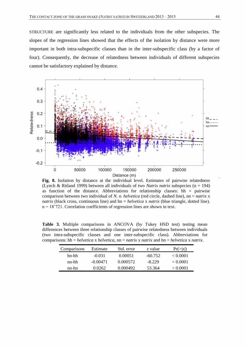
THE CONTACT ZONE OF THE GRASS SNAKE (NATRIX NATRIX) IN SWITZERLAND 2013 – 2015 44
STRUCTURE are significantly less related to the individuals from the other subspecies. The
slopes of the regression lines showed that the effects of the isolation by distance were more
important in both intra-subspecific classes than in the inter-subspecific class (by a factor of
four). Consequently, the decrease of relatedness between individuals of different subspecies
cannot be satisfactory explained by distance.
Comparisons Estimate Std. error z value Pr(>|z|)
hn-hh -0.031 0.00051 -60.752 < 0.0001
nn-hh -0.00471 0.000572 -8.229 < 0.0001
nn-hn 0.0262 0.000492 53.364 < 0.0001
Table 3. Multiple comparisons in ANCOVA (by Tukey HSD test) testing mean
differences between three relationship classes of pairwise relatedness between individuals
(two intra-subspecific classes and one inter-subspecific class). Abbreviations for
comparisons: hh = helvetica x helvetica, nn = natrix x natrix and hn = helvetica x natrix.
Fig. 8. Isolation by distance at the individual level. Estimates of pairwise relatedness
(Lynch & Ritland 1999) between all individuals of two Natrix natrix subspecies (n = 194)
as function of the distance. Abbreviations for relationship classes: hh = pairwise
comparison between two individual of N. n. helvetica (red circle, dashed line), nn = natrix x
natrix (black cross, continuous line) and hn = helvetica x natrix (blue triangle, dotted line).
n = 18’721. Correlation coefficients of regression lines are shown in text.
hh
hn
nn
THE CONTACT ZONE OF THE GRASS SNAKE (NATRIX NATRIX) IN SWITZERLAND 2013 – 2015 45
3.3. MORPHOLGY
3.3.1. Univariate analyses
Statistical significant differences were found in both sexes for 10 variables. They concern the
relative position of the reduction from 19 to 17 dorsal scale rows (X.RNS), the contact between
the temporal and the lower post-ocular scale (C.T.PO), maximum number of post-temporal
scales (PT.MAX), lateral blotches surface (LB.S), lateral blotches length (LB.L), lateral
blotches width (LB.W), nuchal marking size (NM.S.MEAN), nuchal marking length
(NM.L.MEAN), nuchal marking shape (NM.SH) and finally the degree of separation of the
parietal scales and nuchal markings (DS.P.NM). Four variables were significantly different
only among females. They concern the relative head length (X.HL), the relative head width
(X.HW), the head shape (H.S) and the number of gular scales (G). Three significantly different
variables were found between males only, it concerns the relative tail size (X.TL), the number
of paired subcaudal scales (SC) and the body shape (X.WGT).
The comparison of females of the two subspecies shows significant differences for 14 out of 19
criteria (see table A4 [Annexes] for detailed results). The comparison of males shows
significant difference for 13 out of 19 criteria (see table A5 [Annexes] for detailed results).
In addition to the 19 criteria mentioned here above, the patterns of the lunar marking show
relevant divergence between the subspecies. Thirty-six individuals (33 helvetica out of 100 and
3 natrix out of 131) had no, or very faded lunar markings. Moreover, the colour of the lunar
marking, generally whitish, tended to be frequently yellowish in natrix individuals (37% of the
natrix individuals with a marking). Yellowish lunar marking exists also in helvetica, but only
in 5.4% of individuals with a marking.
No criterion provides a diagnostic in all cases; overlapping in continuous values and in
categorical variables between the subspecies occurs for the individuals examined for this study.
3.3.2. Multivariate analyse
When all individuals (n = 231), all continuous variables (n = 17) and both sexes were analysed
together, no obvious clustering was observed (Annexes, figure A6). However, the ellipse
containing 70% of individuals helps the understanding: PC1 (21.5% explained variance)
separates subspecies and PC2 (14.4% explained variance) separates sex, confirming sexual
dimorphism and justifying subsequent analyses with sexes separated.
THE CONTACT ZONE OF THE GRASS SNAKE (NATRIX NATRIX) IN SWITZERLAND 2013 – 2015 46
Females of both subspecies, when analysed with 17 variables (n = 139), showed a potential
discrimination with PC1 (22.5% explained variance), especially for variables: G, H.S, X.RNS,
X.HL, NM.S.MEAN, DS.P.NM, X.HW, NM.SH, NM.L.MEAN, LB.S and LB.L (Annexes,
figure A7, A.). These 11 variables contributed for 5% to 12.5% for PC1. These 11 variables
were used in the next step (Annexes, figure A7, B.), where the PC1 scores are mapped in figure
A8 (Annexes), with microsatellite data in base map (n = 139). The PCA with females,
excluding hybrids and those with missing data (n = 97), using these 11 variables, is shown in
figure 9. The figure 10 maps the PC1 of this analysis, combined with microsatellite data and
the contribution of the morphological data to the PC1, in percentages, is shown in table A7
(Annexes). Finally, these 11 variables were selected in two discriminant analyses. The
discriminant analysis with females, including “hybrids” and missing data (n = 139), indicated a
correct assignment of classes in 80.39 % of the cases. The discriminant analysis with females,
excluding "hybrids" and missing data, indicated a correct assignment in 96.67% of the cases.
The PCA in males, using 17 variables (n = 92), shows a potential discrimination with PC1
explaining 23.2% of the variance, essentially obtained through 10 variables: LB.S, LB.L,
NM.L.MEAN, NM.SH, DS.P.NM, LB.W, NM.S.MEAN, DS.LM, X.RNS and SC (Annexes,
figure A9, A.). These 10 variables contribute for 5% to 12.8% for PC1. These 10 variables
were used in the next step (Annexes, figure A9, B.), where the PC1 scores are mapped in figure
A10 (Annexes), combined with microsatellite data. The PCA with males, excluding hybrids
and those with missing data (n = 62), using these 10 variables, is shown in figure 11. The figure
12 maps the PC1 of this analysis, combined with microsatellite data and the contribution of the
morphological data to the PC1, in percentages, is shown in table A8 (Annexes). Finally, these
10 variables were selected in two discriminant analyses. The discriminant analysis with males,
including “hybrids” and missing data, indicated correct assignment of classes in 91.88 % of the
cases. The discriminant analysis with males, excluding “hybrids” and missing data, indicated a
correct assignment in 91.9 % of the cases. Finally, the morphological variation with only one
variable in both sexes was shown in figure 13. The lateral blotches size was chosen because it
showed good potential of discrimination in females and in males (Annexes, tables A7 and A8).
In summary, the ability to discriminate these subspecies was efficient, for males in 91.9% of
the cases with 10 variables, for females in 96.67% of the cases with 11 variables. The variables
with the higher ability to discriminate the subspecies were mainly the lateral blotches surface
(LB.S) and length (LB.L) (two variables highly correlated) in both sexes. Additionally the
nuchal marking length (NM.L.MEAN), shape (NM.SH) and size (NM.S.MEAN), the degree of
THE CONTACT ZONE OF THE GRASS SNAKE (NATRIX NATRIX) IN SWITZERLAND 2013 – 2015 47
separation between the parietal scales and the nuchal markings (DS.P.NM) and the relative
position of the reduction from 19 to 17 dorsal scale rows (X.RNS) presented also a good
potential of discrimination in both sexes. The relative head width (X.HW), length (X.) and
shape (H.S) (three variables correlated) and the number of gular scales (G) presented a good
potential for discrimination for females only. The lateral blotches width (LB.W), the degree of
separation of the pair of lunar markings (DS.LM) and the number of subcaudal scales (SC)
contributed to discriminate these taxa for the males only.
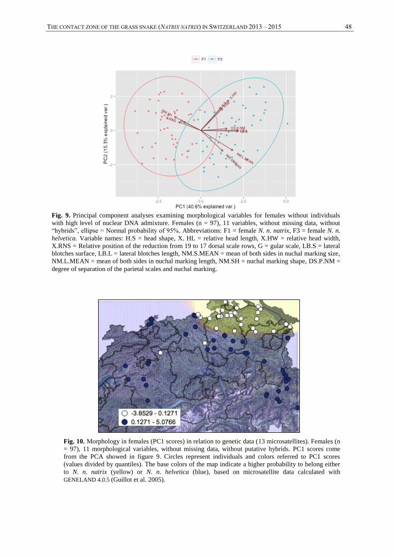
THE CONTACT ZONE OF THE GRASS SNAKE (NATRIX NATRIX) IN SWITZERLAND 2013 – 2015 48
Fig. 10. Morphology in females (PC1 scores) in relation to genetic data (13 microsatellites). Females (n
= 97), 11 morphological variables, without missing data, without putative hybrids. PC1 scores come
from the PCA showed in figure 9. Circles represent individuals and colors referred to PC1 scores
(values divided by quantiles). The base colors of the map indicate a higher probability to belong either
to N. n. natrix (yellow) or N. n. helvetica (blue), based on microsatellite data calculated with
GENELAND 4.0.5 (Guillot et al. 2005).
Fig. 9. Principal component analyses examining morphological variables for females without individuals
with high level of nuclear DNA admixture. Females (n = 97), 11 variables, without missing data, without
“hybrids”, ellipse = Normal probability of 95%. Abbreviations: F1 = female N. n. natrix, F3 = female N. n.
helvetica. Variable names: H.S = head shape, X. HL = relative head length, X.HW = relative head width,
X.RNS = Relative position of the reduction from 19 to 17 dorsal scale rows, G = gular scale, LB.S = lateral
blotches surface, LB.L = lateral blotches length, NM.S.MEAN = mean of both sides in nuchal marking size,
NM.L.MEAN = mean of both sides in nuchal marking length, NM.SH = nuchal marking shape, DS.P.NM =
degree of separation of the parietal scales and nuchal marking.

THE CONTACT ZONE OF THE GRASS SNAKE (NATRIX NATRIX) IN SWITZERLAND 2013 – 2015 49
Fig. 11. Principal component analyses examining morphological variables for males without individuals with
high level of nuclear DNA admixture. Males (n = 62), 10 variables, without missing data, without “hybrids”,
ellipse = Normal probability of 95%. Abbreviations: M1 = male N. n. natrix, M3 = male N. n. helvetica.
Variable names: SC = paired subcaudal scales, X.RNS = Relative position of the reduction from 19 to 17 dorsal
scale rows, LB.S = lateral blotches surface, LB.L = lateral blotches length, LB.W = lateral blotches width,
NM.S.MEAN = mean of both sides in nuchal marking size, NM.L.MEAN = mean of both sides in nuchal
marking length, NM.SH = nuchal marking shape, DS.P.NM = degree of separation of the parietal scales and
nuchal marking, DS.LM = degree of separation of the pair of lunar marking.
Fig. 12. Morphology in males (PC1 scores) in relation to genetic data (13 microsatellites). Males (n = 62),
10 morphological variables, without missing data, without putative hybrids. PC1 scores come from the PCA
showed in figure 11. Circles represent individuals and colors referred to PC1 scores (values divided by
quantiles). The base colors of the map indicate a higher probability to belong either to N. n. natrix (yellow)
or N. n. helvetica (blue), based on microsatellite data calculated with GENELAND 4.0.5 (Guillot et al. 2005).
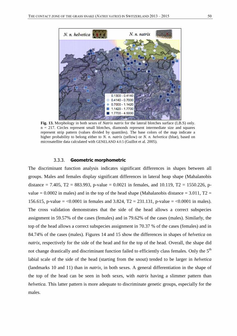
THE CONTACT ZONE OF THE GRASS SNAKE (NATRIX NATRIX) IN SWITZERLAND 2013 – 2015 50
3.3.3. Geometric morphometric
The discriminant function analysis indicates significant differences in shapes between all
groups. Males and females display significant differences in lateral heap shape (Mahalanobis
distance = 7.405, T2 = 883.993, p-value = 0.0021 in females, and 10.119, T2 = 1550.226, p-
value = 0.0002 in males) and in the top of the head shape (Mahalanobis distance = 3.011, T2 =
156.615, p-value = <0.0001 in females and 3.824, T2 = 231.131, p-value = <0.0001 in males).
The cross validation demonstrates that the side of the head allows a correct subspecies
assignment in 59.57% of the cases (females) and in 79.62% of the cases (males). Similarly, the
top of the head allows a correct subspecies assignment in 70.37 % of the cases (females) and in
84.74% of the cases (males). Figures 14 and 15 show the differences in shapes of helvetica on
natrix, respectively for the side of the head and for the top of the head. Overall, the shape did
not change drastically and discriminant function failed to efficiently class females. Only the 5th
labial scale of the side of the head (starting from the snout) tended to be larger in helvetica
(landmarks 10 and 11) than in natrix, in both sexes. A general differentiation in the shape of
the top of the head can be seen in both sexes, with natrix having a slimmer pattern than
helvetica. This latter pattern is more adequate to discriminate genetic groups, especially for the
males.
Fig. 13. Morphology in both sexes of Natrix natrix for the lateral blotches surface (LB.S) only.
n = 217. Circles represent small blotches, diamonds represent intermediate size and squares
represent strip pattern (values divided by quantiles). The base colors of the map indicate a
higher probability to belong either to N. n. natrix (yellow) or N. n. helvetica (blue), based on
microsatellite data calculated with GENELAND 4.0.5 (Guillot et al. 2005).

THE CONTACT ZONE OF THE GRASS SNAKE (NATRIX NATRIX) IN SWITZERLAND 2013 – 2015 50
x3
x1 ♀
x3 ♀
x1
x3
x3
♂
♂
Fig. 14. Shape differences in head of grass snake. Analyses on the side of the head compared 38 females natrix with 28 females helvetica
(A.) and 41 males natrix with 24 males helvetica (B.). Dots are mean position for the group natrix and lines show deformation between
helvetica on natrix. The changes in shapes were amplified with a factor of 3 to improve visibility in the two lower diagrams. Means
comparisons were made with MorphoJ.
A. B.
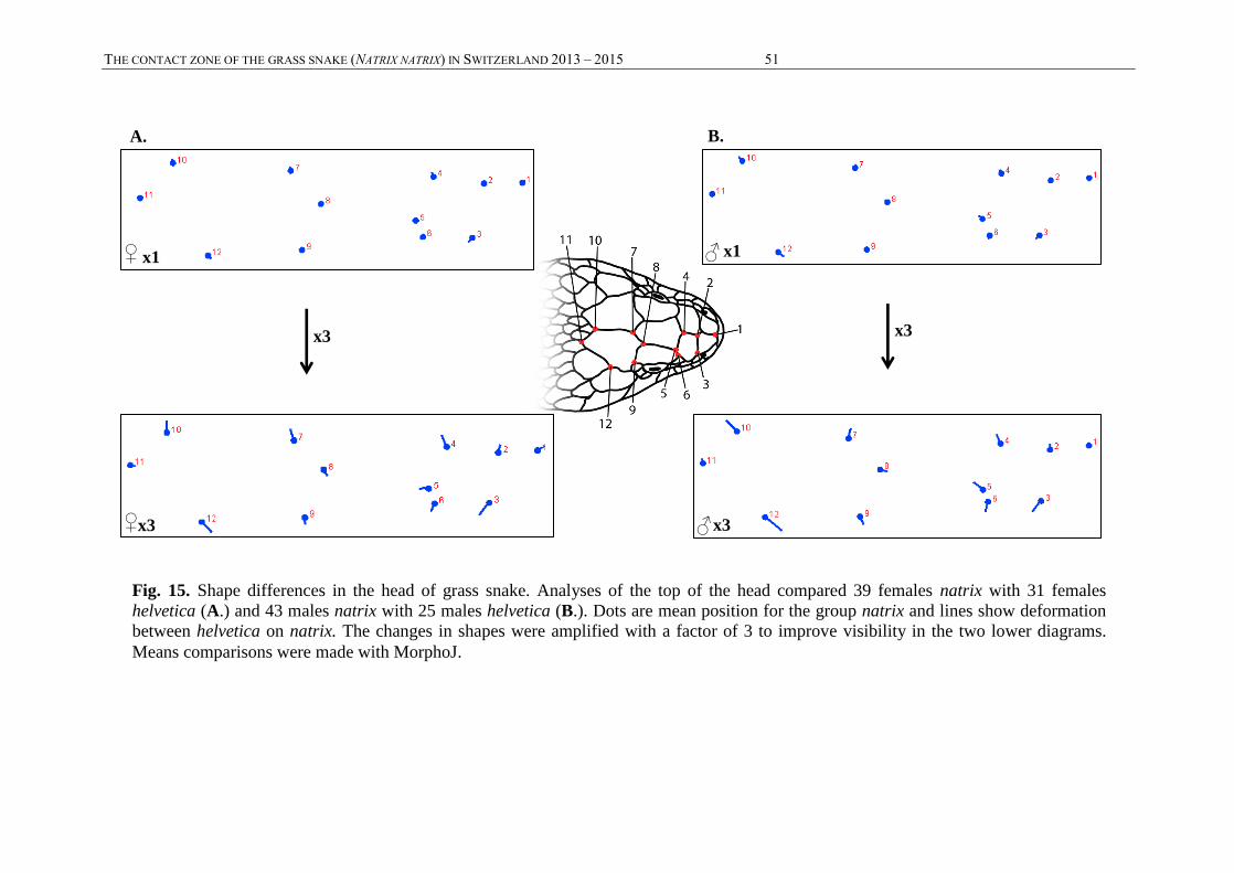
THE CONTACT ZONE OF THE GRASS SNAKE (NATRIX NATRIX) IN SWITZERLAND 2013 – 2015 51
x3 x3
x3 x3
♂
♂
♀
♀
x1 x1
Fig. 15. Shape differences in the head of grass snake. Analyses of the top of the head compared 39 females natrix with 31 females
helvetica (A.) and 43 males natrix with 25 males helvetica (B.). Dots are mean position for the group natrix and lines show deformation
between helvetica on natrix. The changes in shapes were amplified with a factor of 3 to improve visibility in the two lower diagrams.
Means comparisons were made with MorphoJ.
A. B.

THE CONTACT ZONE OF THE SWISS GRASS SNAKE (NATRIX NATRIX) 2013 - 2015 52
Part four
DISCUSSION
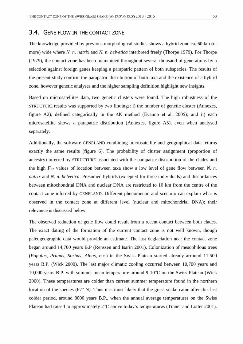
THE CONTACT ZONE OF THE SWISS GRASS SNAKE (NATRIX NATRIX) 2013 - 2015 53
3.4. GENE FLOW IN THE CONTACT ZONE
The knowledge provided by previous morphological studies shows a hybrid zone ca. 60 km (or
more) wide where N. n. natrix and N. n. helvetica interbreed freely (Thorpe 1979). For Thorpe
(1979), the contact zone has been maintained throughout several thousand of generations by a
selection against foreign genes keeping a parapatric pattern of both subspecies. The results of
the present study confirm the parapatric distribution of both taxa and the existence of a hybrid
zone, however genetic analyses and the higher sampling definition highlight new insights.
Based on microsatellites data, two genetic clusters were found. The high robustness of the
STRUCTURE results was supported by two findings: i) the number of genetic cluster (Annexes,
figure A2), defined categorically in the ∆K method (Evanno et al. 2005); and ii) each
microsatellite shows a parapatric distribution (Annexes, figure A5), even when analysed
separately.
Additionally, the software GENELAND combining microsatellite and geographical data returns
exactly the same results (figure 6). The probability of cluster assignment (proportion of
ancestry) inferred by STRUCTURE associated with the parapatric distribution of the clades and
the high FST values of location between taxa show a low level of gene flow between N. n.
natrix and N. n. helvetica. Presumed hybrids (excepted for three individuals) and discordances
between mitochondrial DNA and nuclear DNA are restricted to 10 km from the centre of the
contact zone inferred by GENELAND. Different phenomenon and scenario can explain what is
observed in the contact zone at different level (nuclear and mitochondrial DNA); their
relevance is discussed below.
The observed reduction of gene flow could result from a recent contact between both clades.
The exact dating of the formation of the current contact zone is not well known, though
paleogeographic data would provide an estimate. The last deglaciation near the contact zone
began around 14,700 years B.P (Renssen and Isarin 2001). Colonization of mesophilous trees
(Populus, Prunus, Sorbus, Alnus, etc.) in the Swiss Plateau started already arround 11,500
years B.P. (Wick 2000). The last major climatic cooling occurred between 10,700 years and
10,000 years B.P. with summer mean temperature around 9-10°C on the Swiss Plateau (Wick
2000). These temperatures are colder than current summer temperature found in the northern
location of the species (67° N). Thus it is most likely that the grass snake came after this last
colder period, around 8000 years B.P., when the annual average temperatures on the Swiss
Plateau had raised to approximately 2°C above today’s temperatures (Tinner and Lotter 2001).
THE CONTACT ZONE OF THE SWISS GRASS SNAKE (NATRIX NATRIX) 2013 - 2015 54
Simulation based on dispersal distance, dispersal pattern, mate frequency, generation time,
selection against genes and on an adapted data set would be required to assess whether 8000
years of contacts are enough to infer a stable equilibrium in gene exchanges between both
subspecies. Currently, only the number of generations since the contact zone formation is
available. According to Lande et al. (2003), generation time is defined as:
T = α+ [s/1*(1-s)]
where α is the age at the first reproduction and s is the adult annual survival. For the grass
snake α = 4 years and s = 0.48 (Madsen 1987). Thus generation time is T = 4+ [0.48/1*(1-
0.48)] = 4.25 years corresponding to ca. 1900 generations (against ca. 3000 for Thorpe 1979).
Such a large number of generations support the hypothesis that the equilibrium is probably
already reached. This could not be the case, whether the grass snake is sedentary (in both
sexes), with a very low dispersal power, thus total nuclear genome homogenization would have
taken a lot of time, if occurring. However, this seems unlikely regarding the high mobility of
the species. Indeed, Meister et al. (2012) found a high gene flow between populations of N. n.
helvetica separated by 10 and 30 km along the Aare River (FST values between 0.02 and 0.08;
mean of 0.085 in the present study). The authors also argued that the low rate of animal
recapture could corroborate this purpose.
However, the high mobility of the grass snake only inferred by nuclear markers cannot
highlight the dispersal pattern of the species. For instance, a sedentary behaviour of females
can lead to a low dispersal power and consequently to a parapatric distribution of mtDNA.
Bonnet et al. (1999) found more females (n = 23) than males (n = 7) killed by natural predator
and anthropogenic sources of mortality as roadkill in genus Natrix (combined data on N. maura
and N. natrix). The authors explained their finding of a highest rate of snakes killed during the
egg-laying by a need for the females to reach an oviposition site. Thus, the results suggest a
higher mobility of the females than males. However, if they always choose the same
oviposition site, their behaviour would not contribute to genes dispersal. Although Reading and
Jofré (2009) tracked a female that hibernated at the same site during the 2 years of the research,
their findings, based on one individual only, is anecdotal. The other existing studies, based on
radio tracking, do not contribute to an answer because they were usually conducted during one
season only and never focused on the dispersal ability of the grass snake (Madsen 1984, Wisler
et al. 2008, Reading and Jofré 2009). Madsen (1987) stressed the difficulty to separate
mortality and dispersal components in in capture-recapture studies. Thus no consistent data are
THE CONTACT ZONE OF THE SWISS GRASS SNAKE (NATRIX NATRIX) 2013 - 2015 55
available to infer dispersal behaviour in females. In the other sex, the available data are
equivalent. The difficulties are similar in studies considering the males. Only two males were
successfully radio tracked in the literature: one by Madsen (1984) in Sweden and one by
Reading and Jofré (2009) in England. Madsen showed high movements during May-June
mating season (mean of 55 m per day) and a more sedentary behaviour later in the season
(mean of 13 m per day in July). Reading and Jofré (2009) concentrated on collecting data over
several seasons but could track one male only for one and a half season. They showed that this
individual stayed at the same locations during two consecutive years. Unfortunately, the above-
mentioned information, too poor in data, cannot conclude to specific different female or male
philopatric patterns (i.e. which sex migrate or stay), if such patterns exist. The data set of the
present study did not allow testing sex-biased dispersal because it was not centered at the
population level. Consequently, it is not possible at this stage to explain the low level of
mtDNA overlapping in the female distribution by a specific sedentary behavior. Although all
hypotheses can be envisaged, the relative high nuclear flow between populations (see above)
indicates that if the females are sedentary, then males have probably a great dispersal power.
Locations and maintaining of hybrid zones can be explained by ecological transition (Swenson
2006). In reptiles, such pattern has been found in three viper species in Spain (Tarroso et al.
2014). This explanation seems unlikely in the case of the grass snake as no evident difference
in ecology between subspecies have been highlighted. Two different studies on the grass snake
diet displayed similar results in Sweden (Madsen 1983; taxon: N. n. natrix) and in Italy (Filippi
et al. 1996; taxon: N. n. helvetica or N. n. lanzai depending on the author). In both cases
females of both subspecies diet on Bufo bufo (common toad) and similar food suggests similar
habitats and similar ecology. Differenciation could depend on abiotic factors as climatic
conditions (e.g. affecting incubating temperature), although no transition in temperature,
elevation, radiation or precipitation was found in the study area. As a comparative study
focusing on differential ecologies of the grass snake subspecies is lacking, an ecological factor
cannot however totally be excluded.
Geographical differentiation within one species is sometimes explained by clines or isolation
by distance (de Queiroz 2007). This explanation is unlikely in the case of the grass snake
regarding the FST and relatedness-based analyses. FST and relatedness results are concordant,
but significant isolation by distance was detected in the relatedness-based analysis only. It was
particularly visible for pairwise relatedness in the intra-subspecies classes (natrix x natrix and
helvetica x hevletica). The slopes of the regression lines show that the isolation by distance has

THE CONTACT ZONE OF THE SWISS GRASS SNAKE (NATRIX NATRIX) 2013 - 2015 56
an effect, though minor, on the relatedness between individuals within the same subspecies. In
this research on the grass snake, the slope of the inter-subspecies class is 77% gentler than the
slopes of the intra-subspecies classes (figure 8), indicating that the isolation by distance does
not explain the high genetic differentiation between the subspecies.
Sexual behaviour and mate choice are a possible explanation for the reduction in gene flow
between taxa. The female snakes use a pheromone system to attract and motivate the males to
copulate (Shine 2003). In the case of the grass snake, it is possible that, after 7 millions years of
divergence, the bouquet of pheromones presents differences and improve the recognition
among taxa. The reproductive barrier was shown to be semipermeable, especially among the
populations with nuclear admixture in the Canton of Zürich and in the Alpine Rhine Valley.
However, a marginal effect of non-random mating is possible in the very sharp genetic and
morphological transitions in the north of the Canton of Aargau. Along a transect of 7 km
(Euclidian distance) only one individual (GIP02, ancestry proportion = 0.681 for helvetica) out
of 8 helvetica and 11 natrix, presented an ancestry proportion lower than 0.87 and no mtDNA
introgression was detected. So few presumed hybrids encountered within such a little distance
through the centre of the contact zone (knowing that hybrids are viable) can indirectly support
a certain level of mate recognition. In addition, the FST analyses confirm this view. Thorpe
(1979) stated that two pure forms cannot “directly hybridise” because the populations in the
center of the contact zone are made of intermediate forms only. However, the higher definition
found in this study suggests that other conclusions than Thorpe are possible. For example, the
populations in Canton Aargau, with abundant males and females in both subspecies, may favor
the choice of the “good” taxa for mating while areas where more mtDNA introgression and
nDNA admixture are found (e.g. Alpine Rhine Valley) could consist in smaller population,
constraining the interbreeding, potentially induced by disturbed habitats.
When interbreeding between N. n. natrix and N. n. helvetica occurred, genetic admixture
affects the fitness of the offsprings. The hybrids are known to exist and to be viable (mtDNA
introgression is found several individuals and locations in both taxa). Thus, a viable hybrid
with the same fitness of its parent and without mating recognition system will chose randomly
its mating partner. Consequently, after 1900 generations of randomly mating and of unaffected
fitness, the contact zone should be occupied by hybrid populations forming one cluster of
mixed genotypes (Mallet 2006). This occurrence was not observed in this study, even in the
closest populations of the centre of the contact zone. Finally, even if the fitness is slightly
decreased, the high intra-subspecific gene flow (see above) is able to prevent introgression, as
THE CONTACT ZONE OF THE SWISS GRASS SNAKE (NATRIX NATRIX) 2013 - 2015 57
demonstrated by simulations (Petit and Excoffier 2009). Both females and males were found as
putative hybrids, thus there is no evidence for Haldane’s rule (theory showing hybrid
deficiency for the heterogametic sex). Indeed, differentiated sex chromosome is common in
snakes (Phillips and Edmands 2012), and, though this knowledge is missing, there is no
indication of the contrary in the case of the grass snake. The asymmetric sampling between
sexes in this study (86 females and 61 males) might explain that more female hybrids (14) than
males (6) were recovered. Chi-square test found no significant difference in ratio (χ=0.969, df
=1, p-value = 0.32). Hardy-Weinberg equilibrium could not be tested with this dataset because
populations were too small to infer strong statistics, thus, there is no direct evidence for gene
selection in the populations close to the contact zone.
Without requiring intrinsic mechanisms, the geographical barriers potentially existing at the
centre of the contact zone could limit the gene flow between taxa. In the north of the study area
(in the north of the Canton of Aargau), the Aare River coincides well with the inferred contact
zone. However, helvetica individuals were found on both side of this river, suggesting that this
snake can cross such river without difficulties (the grass snake swims very well). The foothills
of the Alps corresponding to the upper valley of the Thur River (Toggenburg region), but also
the upper valley of the Töss River on the Swiss Plateau provide important natural barriers
between both taxa. Helvetica individuals are found west of this barrier and natrix individuals to
the east. Even if this snake becomes rare above 1000 meters, the greatest difficulty for the grass
snake to occupy these areas is the lack of adapted habitat (observations made only close to the
two principal rivers). As there is no geographical barrier neither on the Swiss Plateau (with the
exception of the Toss River), nor at the end of the Alpine Rhine Valley, a sharp contact zone is
maintained, irrelevant of the existence of a geographical barrier.
In short, and even without causal evidence, a decrease of fitness of the hybrids is the logical
explanation for the maintenance of a clear genetic distinction between taxa. The model
advanced by Thorpe (1979) where the two subspecies freely interbreed and where the foreign
genes are progressively removed by selection is stronger than previously expected regarding
the sharpness of the newly defined contact zone. Finally, all the points and hypotheses
discussed here above cannot be totally excluded (for the unlikely ones) or advanced as prior
effect (for the most likely), more probably a combination of several natural processes is
possible to explain this reduction of gene flow between N. n. natrix and N. n. helvetica.
THE CONTACT ZONE OF THE SWISS GRASS SNAKE (NATRIX NATRIX) 2013 - 2015 58
3.5. MORPHOLOGY
Discrimination ability
The majority of the criteria identified by Thorpe (1979) selected for this study were
significantly different (14 on 19 in females and 13 on 19 in males, see in the Annexes, table A4
and A5) between both taxa inferred by the genetic analyses.
No perfect diagnostic character was established. Nevertheless, some characters are potentially
relevant to discriminate the two taxa, particularly when combined. In both sexes, the best
candidates are the lateral blotches (surface and/or length) and the nuchal marking (length and
shape). Additionally, the females show differences in general head shape (metric
measurements) and for the number of gular scales (the other criteria presenting a good potential
for discrimination are available in the Annexes, table A7). In males, the degree of separation of
the lunar markings, the lateral blotches width and the number of subcaudal scales present also a
good potential for discrimination (see the complete list in the Annexes, table A8). The
discriminant analysis for 11 morphological variables indicates a strong ability to correctly class
the individuals to their genetic groups, especially for females (96.67%, n = 97). Surprisingly,
males were less likely to be correctly assigned to their genetic group with 10 morphological
variables (91.9%, n = 62). The smaller dataset (62 individuals) increase the likelihood of a bias
caused by the phenotypic plasticity (non homogenous data sampled by chance). Alternatively,
this difficulty in assignment could also reflect a lower selective pressure on males, leading to a
slower morphological differentiation than in females. This number of samples collected does
not allow to explain adequately this difference. It is interesting to note that Thorpe (1979)
found also a slighter morphologic differentiation in males than in females, which he attributed
to the “paucity of male specimens”.
Strip pattern
The lateral blotches pattern alone is a good candidate to discriminate these genetic groups
(figure 13), as often mentioned in the literature describing these subspecies (e.g. Kabisch
1978). However, this is not a 100% diagnostic character and a combination of several criteria is
required to improve the determination (as the nuchal area pattern). N. n. helvetica with small
blotches are rare and N. n. natrix with a strip pattern were found only in the centre of the
THE CONTACT ZONE OF THE SWISS GRASS SNAKE (NATRIX NATRIX) 2013 - 2015 59
contact zone, but the real problem of these lateral blotches come from a more frequent
intermediate pattern found also in both “pure” taxa (figure 13).
Lunar marking colour
Additionally to the 19 criteria analysed, the presence of a yellowish lunar marking indicates a
N. n. natrix individual (confidence to 95%, n = 119), while the absence of lunar marking
suggests a N. n. helvetica individual (confidence to 91%, n = 119) but the presence of a whitish
lunar marking is largely uninformative for determination purposes at the individual level (66%
in natrix and 79% in helvetica, n = 119).
Occipital marking
The presence and the size of the occipital marking (not measured in this study, but mentioned
by Kabisch 1978) present potentially a good criteria of discrimination, corresponding to the
adjacent and proximal dark marking of the lunar marking (covering in part the last three
supralabial scales, the post-temporal scales, the post-parietal scales, the distal part of the
parietal scale, etc.). This marking is generally absent or very faded in N. n. helvetica,
contrasting with the more pronounced and visible markings in N. n. natrix. A rapid inspection
of the field photographs indicated that this criterion presented a good potential of
discrimination (as complementary criteria).
Geometric morphometric
In geometric morphometric analyses, the photographs of the grass snake heads indicated a
general trend for N. n. natrix to have a slimmer head (viewed from the top). Although this
differentiation is almost imperceptible to the naked eyes, the discriminant functions were able
to assign 84.74 % of the males and 70.37 % of the females to the correct genetic groups.
The analyses of the side of the head show a greater difficulty to discriminate females (59.57%)
than males (79.62%), contradicting the results in multivariate analyses based on body
proportions, scalation and patterns. The large variability in head shapes among females may
explain this contradiction. Allometry should be controlled and/or different age groups should
THE CONTACT ZONE OF THE SWISS GRASS SNAKE (NATRIX NATRIX) 2013 - 2015 60
be separately analysed (total length and head measurements were highly correlated in PCA
analyses).
Hybrids
The analyses including the hybrids are not conclusive. Adding the hybrids (individuals with
ancestry proportion < 0.8) to the analyses decreases the ability to assign correctly the females
by 16.28% (0.01 % for the males). Some of the hybrids were morphologically close to the pure
form, thus they were systematically classed as pure to one or other subspecies increasing the
error rate. Different classes of hybrids need to be treated differently in order to study accurately
such data. One of these different treatment could be the analyse of the correlation between
proportion of ancestry returned by STRUCTURE and morphological scores of PCA. However,
the dataset were not large enough to make such analysis (22 female hybrids and 6 male
“hybrids” only).
Thorpe (1979) identified a population constituted by individuals with an intermediate and
variable morphology at the centre of the contact zone (municipality of Turbenthal, Canton of
Zurich). The results of the present study confirm the presence of hybrid populations in this area
where an introgression event (mtDNA) and a high level of nuclear DNA admixture are found
(populations ZEL and WIN). In this area, only the clade E (N. n. helvetica) is found, although
the nuclear DNA is mainly natrix (in mean, STRUCTURE showed a mean of proportion of
ancestry to 0.8 for natrix, n = 11). The morphological analyses showed also a high
morphological variability in these populations. This could be the result of an old presence of
the taxa helvetica in the valley followed by an “invasion” of natrix males. The alternative
would be that the helvetica females migrated and replaced the local natrix females and their
haplotype. As knowledge is lacking on the dispersal behaviour of this species, more
investigations are needed to solve this specific hybridisation event. The opposite example is
found in population DUB, where the mean of proportion of ancestry in four individuals is 0.97
for helvetica. For this latter population, the morphology corresponded to pure helvetica
(regarding the principal component analysis scores), even the proximity to the contact zone (<
5 km) and the mtDNA introgression (belonging to clade 3 – so N. n. natrix). This suggests an
older hybridization event in population DUB because the nuclear alleles from natrix are now
totally removed. This scenario, where the foreign alleles are totally replaced by those of
another taxa, is potentially occurring in populations ZEL and WIN and is more readily by a
THE CONTACT ZONE OF THE SWISS GRASS SNAKE (NATRIX NATRIX) 2013 - 2015 61
migration of the males. Such hybridisation events can be the result of natural movement of the
contact zone and migration events, but can also result from human-induced disturbance. It
could be the case, for example, after the constructions of highway (which began in the sixties in
Switzerland) and causing isolation of small population, forcing them to interbreed with the
other taxa. However, the present study cannot confirm such conclusions.
3.6. TAXONOMIC REASSESSMENT
The relative concordance between mitochondrial DNA, nuclear DNA and morphological
results suggests the existence of two evolutionary/taxonomic entities, that live in parapatry and
form a thin hybrid zone crossing the northeast of the Switzerland. These results confirm, in
part, the previous findings of Thorpe (1979), who anticipated the existence of a hybrid zone
crossing the northeast Switzerland with a relative accuracy. However, the sharpness of the
newly defined contact zone highlighted by genetic tools shows that the selection against mixed
genotype is stronger than previously expected.
The integrative taxonomy considers the possibility to speak of about species when one or more
lines of evidence are found (see the introduction: Emergent concepts). In the present case,
concordance occurs for the three taxonomic characters studied (mtDNA, nDNA and
morphology) with some nuances at the contact zone. Mitochondrial DNA introgression is
found at a distance of less than 10 km to the contact zone inferred with nuclear DNA. The
nuclear DNA admixture is important in populations closer than 5 km to the contact zone
(without being systematic), and gradually disappears between 10 to 20 km from the contact
zone. Finally, the high variability in morphology induced a lack of diagnostic characters at the
individual level; however a combination of several characters provides a strong discrimination
power in concordance with the nuclear DNA, especially in females.
In addition to the congruence between different and independent taxonomic characters to
delineate species, several authors agree that evidence for partial or complete reproductive
isolation is probably the most important feature in the recognition of distinct species (Cracraft
1989, Meiri & Mace 2007, Padial et al. 2010, Hausdorf 2011, Frankham et al. 2012). Partial or
complete reproductive isolation ensures the genetic integrity of lineages (maintained
throughout times) and suggests distinct evolutionary fate (sensu Wiley 1978). The limited
contact zone detected with nuclear markers strongly suggests the existence of intrinsic
mechanisms preventing the merging of both lineages (maintained after ca. 2000 generations).
THE CONTACT ZONE OF THE SWISS GRASS SNAKE (NATRIX NATRIX) 2013 - 2015 62
The most likely explanation is a decrease of the fitness of the hybrids, but prezygotic isolation
cannot be totally excluded without additional investigations. For Hausdorf (2011), evidence for
a decrease of the fitness of the hybrids is the only condition required to separate species.
Thus, the concordance between mitochondrial DNA, nuclear DNA and morphology, with
nuances at the contact zone due to the presence of the hybrids, and the indirect evidence of the
unfitness of the hybrids suggest that N. n. natrix and N. n. helvetica can be regarded as separate
species. Such conclusion will induce the changes of name in Natrix natrix for Natrix natrix
natrix and Natrix helvetica for Natrix natrix helvetica. The biological species concept (sensu
Mayr 1942) causes real difficulties to this conclusion; thus it is important to precise that both
taxa are not “biological species”, but rather distinct “evolutionary lineages” preventing from
merging. As discussed in the introduction, the biological species concept cannot be seen as the
prior concept regarding the current understanding about speciation and hybridisation. Indeed,
hybridisation does not act as an obstacle to speciation when it is shown that the gene flow is
reduced between several biological/taxonomic entities.
3.7. NEXT RED LIST OF REPTILES OF SWITZERLAND AND CONSERVATION
IMPLICATIONS
Taxonomy
The recognition of the species status of Natrix natrix and Natrix helvetica induces some
conservation implications. The next Red List of the reptiles of Switzerland will have to
consider both taxa as distinct species. Thus, the monitoring and the follow up of the size, health
and connectivity of populations should be conducted separately.
Area of occupancy
Based on the microsatellite results the area of occupancy of both taxa is now known with
accuracy. The morphology, which has been used in the last Red List to calculate the area of
occupancy, coincides well with the genetic. Thus, the size of areas of both taxa should not
significantly change. This implies that without important decline in population size since the
last Red List, the threat status should not change in both taxa.
THE CONTACT ZONE OF THE SWISS GRASS SNAKE (NATRIX NATRIX) 2013 - 2015 63
Conservation actions
In the case of future conservation plan such as translocation of animals to improve genetic
diversity of specific populations, the interbreeding between these two taxa will be probably
damaging for the local population. A previous study on the fitness of the offspring resulting
from such interbreeding is strongly recommended. Indeed, the present results suggest a
decrease of fitness of the hybrids.
IUCN
Before to extrapolate these results at an international level, additional studies are needed in
other countries crossed by the contact zone (Austria, Germany and Italy) as the existence of a
very sharp contact zone in one location and of the very diffuse in another location is possible,
as in the special case of ring species (Joseph et al. 2008). A ring species means that two
populations behave as apparently well differentiated entities (with a total or a partial
reproductive barrier) in a specific area but are connected by a chain of integrating populations
in other areas of its range (causing taxonomic difficulties). For instance in the grass snake,
Thorpe (1979), found a higher morphological variation in the contact zone in the Po Valley
(Italy); thus this area could be very predestined to validate the present conclusion.
3.8. PERSPECTIVE
Unfitness of the hybrids
This study strongly suggested a fitness decrease of the hybrids. To get a direct confirmation,
studies based on the complete and successful maturation of embryos should be considered, for
instance with eggs collected in the natural contact zone and juvenile released after hatching.
The count of the number of half-ventral scales, which are directly associated with imperfect
embryogenesis and asymmetric internal morphology, can also be evaluated; this parameter is
correlated with the fitness of the successfully born grass snakes (Löwenborg et al. 2011). The
decrease in fitness was measured with changes in anti-predator behaviour, in body length and
in locomotion speed and was explained by non-optimal temperature during the embryogenesis.
Such data collection could be informative in the hypothetical case of hybrids failing to find

THE CONTACT ZONE OF THE SWISS GRASS SNAKE (NATRIX NATRIX) 2013 - 2015 64
adapted egg-laying sites and showing more half-scales in proportion at the contact zone. This
could be achieved in the Alpine Rhine Valley, where a high level of nuclear DNA admixture
has been detected. Additionally, experimentation in laboratory to test mate choice could be
achieved. This would be particularly relevant to know if prezygotic barrier can act, at least
partially, as barrier to the gene flow (confirming a supplementary step in their evolutionary
divergence). Finally, the fecundity rate and the number of eggs produced when interbreeding
occurs between both taxa could be also tested in laboratory.
The Italian clade
The haploclade C detected in Ticino (also present in Italy, according to Kindler et al. 2013) has
been voluntary put aside from the results and the discussion. This single individual corresponds
to a supplementary phylogeographic condition and, being alone, was anecdotal in this study.
However, this individual (MUE05) has been successfully genotyped and STRUCTURE
considered it as close to the helvetica taxon (proportion of ancestry for helvetica to 0.76) while
the software GENELAND considered it as an individual from a third population. The Alps
present necessarily a strong barrier to the gene flow and the preliminary microsatellite analyses
suggests that this lineage just possesses some private alleles. Further studies are welcome in the
east Po Valley where clade C and 3 (natrix) potentially meet (and where similarity with the
Swiss contact zone is expected) and potentially where clade C and E (helvetica) meet (where
higher nDNA admixture and mtDNA introgression is expected).
Morphology
Even with several morphological characters, it is difficult to assign individuals to one or
another taxa close to the contact zone based on morphology alone due to the inability to
perform robust statistics with the few hybrids available in this study. A study focusing on
locations where both taxa meet (e.g. Alpine Rhine Valley), with a larger sample size, could
potentially help for the determination of the hybrids. Moreover, the present study used non-
standardized method for the morphological measures, except for the body proportions and the
scalation pattern. The eye estimation used for the colour patterns provides good information on
the existence of morphological differentiation, but cannot be used for an accurate determination
by a third party. A solution could be to take photographs at a known scale and to measure the
criteria with numeric tools (for example with the freeware and user-friendly ImageJ). Such
THE CONTACT ZONE OF THE SWISS GRASS SNAKE (NATRIX NATRIX) 2013 - 2015 65
method is computer time consuming, but saves time on the field and limits manipulations of the
animal.
Differential ecology and behaviour
Studies focusing on the ecology and/or on the behaviour of the distinct subspecies of the grass
snake are lacking. It would not be surprising that N. n. natrix and N. n. helvetica have acquired
differential adaptations due to the long time divergence since their separation, their different
phylogeographic history and their current confirmed evolutionary independence.
Additional population-based studies
A design based on populations (for example by collecting 30 individuals by populations on
three different locations) would be more adapted to better define the age of the contact zone
and the rate of migration between taxa. This means, in practice, one population of N. n. natrix
located close to the contact zone, one population at a location where both taxa meet frequently
and one population of N. n. helvetica population also close to the contact zone. The rate of
migration could be evaluated with a software such as MIGRATE-N (Beerli and Felsenstein 2001)
and the age of the contact zone inferred by approximate Bayesian computation (ABC)
approaches. Such approach would also allow testing Hardy-Weinberg equilibrium indicating
direct evidences for gene selection in the populations close to the contact zone. Finally, the sex-
bias dispersal could be tested to know if a particular philopatric pattern exists.

THE CONTACT ZONE OF THE SWISS GRASS SNAKE (NATRIX NATRIX) 2013 - 2015 66
Part five
CONCLUSION
THE CONTACT ZONE OF THE SWISS GRASS SNAKE (NATRIX NATRIX) 2013 - 2015 67
Thorpe (1979) discovered, with an intensive morphological analysis, a contact zone crossing
the middle Europe where two forms of grass snakes meet and are viewed as “incipient species”.
However, all phylogeographic studies on this species postulated that the model of the four
subspecies considered by Thorpe underestimate genetic diversity of the grass snake and
demand a taxonomic revision of the species (Guicking et al. 2006, Fritz et al. 2012, Kindler et
al. 2013). The results of the present study confirm that these two subspecies are two distinct
evolutionary units (starting their divergence ca. 7 millions years ago). The results of the present
study support the Thorpe’s findings, although modern tools and the large sample on a close
area provided new insights on the nature of the hybrid zone. Indeed, the narrowness of the
contact zone inferred by nuclear DNA data (13 microsatellites), the mtDNA introgression
limited at 10 km to the contact zone and the concordance with the morphology suggest a
greater differentiation as expected by Thorpe (1979).
The large number of generations since the formation of the contact zone suggests that both
evolutionary lineages are prevented from merging and undoubtedly highlights a point of no
return in their evolutionary divergence. The tight genetic transition observed between taxa is
probably the result of a decrease in fitness of the hybrids, although no direct evidence currently
exists. All these elements support a distinction of both taxa as separate species. This distinction
would have implication on the conservation of these snakes in Switzerland as differential
monitoring and follow up in the future would be required, and a change in the taxonomic status
in the next Red List of the reptiles of Switzerland. However, the threat level of both taxa should
probably not change from Monney and Meyer (2005) due to the concordance between
morphology (used for previous monitoring) and genetic. Indeed, the surface of occupancy,
which will be calculated in the next Red List based on new genetic results, should not
significantly change.
In confirming and ensuring two different evolutionary lineages, regarded as distinct species in
the future, this study shows the relevance to take into consideration infraspecific taxonomic
level for conservation purpose (as already considered in Monney and Meyer 2005). Subspecies
do not represent systematically slight geographical variations within a species, but potentially
hide strong and unexpected differentiated entities, even without strong and obvious
morphological or ecological differences.
The morphological analyses showed that pure female were distinguishable up to 96.67% and
the males up to 91.9% with, respectively, 11 and 10 characters. This results show a good
potential to recognize the genetic groups without molecular analysis. The lateral blotches
THE CONTACT ZONE OF THE SWISS GRASS SNAKE (NATRIX NATRIX) 2013 - 2015 68
pattern is the better candidate to assign individual to one or other taxa, but a combination of
several criteria is strongly recommended (as the nuchal area patterns).
Finally, this study shows the importance to work at fine scale to study contact zones. A
collection of sample at locations separated by 20 km, for example, would probably have
prevented collecting hybrids while the presence of these hybrids confirms the view that species
must not be seen as totally autonomous and that speciation occurs despite ongoing
interbreeding.

THE CONTACT ZONE OF THE SWISS GRASS SNAKE (NATRIX NATRIX) 2013 - 2015 69
3.8.1. Acknowledgments
I wish to thank S. Ursenbacher for his time, his help and his precious advises that he has given
to me over the course of this work.
A thank for having accompanied me in the field, advised in the laboratory or for all other kinds
of help to S. Ursenbacher, V. Zwahlen, G. Guex, H. Schmocker, H. G. M. Chèvre, S. F.
Chèvre, R. Jacobi, G. Fatton, J. Frutschi, B. Erne, J. Gurtner, D. Jacobi, M. Voordouw, H.
Billing and J.-P. Corboz.
Thanks to A. Meyer, B. Meister, B. Schmidt, B. Erne, G. Dusej, J. Barandun, K. Mebert, M.
Tschofen, M. Frei, N. Peyer, P. Leuthardt, R. Neumeyer and S. Ursenbacher for supplementary
DNA material.
I am grateful to the Institut für Natur-, Landschafts- und Umweltschutz (NLU) of Basel for
having made available its molecular laboratory.
I would like to thank the Natural History Museums of Basel, Bern, Chur, Geneva, Zurich and
many more to have answered to my requests.
Sincere thanks to the Cantons of Aargau, Glarus, Grisons, Lucerne, Schaffhausen, Schwytz, St.
Gallen, Thurgau and Zurich for having issued the authorizations for sampling and catching
animals.
I gratefully acknowledge the financial support from the Federal Office for the Environment.
A very special thank to the persons managing the natural reserve in Switzerland who think to
favour this (or rather these) species abandoning voluntary large piles of wood and for the
numerous human-build egg-laying sites met which have facilitated my field work!
Finally, I would like to pay tribute to the late J.-C. Monney who has passed on to me a small
part of his immense passion of the reptiles during two unforgettable excursions in 2012.

THE CONTACT ZONE OF THE SWISS GRASS SNAKE (NATRIX NATRIX) 2013 - 2015 70
Part six
BIBLIOGRAPHY
THE CONTACT ZONE OF THE SWISS GRASS SNAKE (NATRIX NATRIX) 2013 - 2015 71
Agapow, P. M., Bininda‐ Emonds, O. R., Crandall, K. A., Gittleman, J. L., Mace, G. M., Marshall, J. C., &
Purvis, A. (2004). The impact of species concept on biodiversity studies. The quarterly review of
biology, 79(2), 161-179.
Arias, C. F., Rosales, C., Salazar, C., Castaño, J., Bermingham, E., Linares, M., & McMillan, W. O. (2012). Sharp
genetic discontinuity across a unimodal Heliconius hybrid zone. Molecular ecology, 21(23), 5778-5794.
Beerli, P., & Felsenstein, J. (2001). Maximum likelihood estimation of a migration matrix and effective population
sizes in n subpopulations by using a coalescent approach. Proceedings of the National Academy of
Sciences, 98(8), 4563-4568.
Blouin-Demers, G., & Gibbs, H. L. (2003). Isolation and characterization of microsatellite loci in the black rat
snake (Elaphe obsoleta). Molecular Ecology Notes, 3(1), 98-99.
Bonnet, X., Naulleau, G., & Shine, R. (1999). The dangers of leaving home: dispersal and mortality in
snakes. Biological conservation, 89(1), 39-50.
Bromham, L. (2002). Molecular clocks in reptiles: life history influences rate of molecular evolution. Molecular
biology and evolution, 19(3), 302-309.
Burbrink, F. T., Lawson, R., & Slowinski, J. B. (2000). Mitochondrial DNA phylogeography of the polytypic
North American rat snake (Elaphe obsoleta): a critique of the subspecies concept. Evolution, 54(6), 2107-
2118.
Burns, E. L., & Houlden, B. A. (1999). Isolation and characterization of microsatellite markers in the broad-
headed snake Hoplocephalus bungaroides.Molecular Ecology, 8(3), 520-521.
Clement, M., Posada, D. and Crandall, K. (2000). TCS: a computer program to estimate gene genealogies.
Molecular Ecology 9(10): 1657-1660
Cracraft, J. (1989). Speciation and its ontology: the empirical consequences of alternative species concepts for
understanding patterns and processes of differentiation. Speciation and its Consequences, 28-59.
Cracraft, J. (2000). Species concepts in theoretical and applied biology: a systematic debate with
consequences. Species concepts and phylogenetic theory: A debate, 1-14.
Crandall, K. A., Bininda-Edmonds, O. R. P., Mace, G. M., & Wayne, R.K. (2000) : Considering evolutionary
processes in conservation biology. Trends in Ecology & Evolution 15 : 290–295.
Dayrat, B. (2005). Towards integrative taxonomy. Biological Journal of the Linnean Society, 85(3), 407-415.
De Queiroz, K. (2007). Species concepts and species delimitation. Systematic biology, 56(6), 879-886.
DeSalle, R., Egan, M. G., & Siddall, M. (2005). The unholy trinity: taxonomy, species delimitation and DNA
barcoding. Philosophical Transactions of the Royal Society of London B: Biological Sciences, 360(1462),
1905-1916.
Dobzhansky, T. (1970). Genetics of the evolutionary process (Vol. 139). New York: Columbia University Press.
Dong, S., & Kumazawa, Y. (2005). Complete mitochondrial DNA sequences of six snakes: phylogenetic
relationships and molecular evolution of genomic features. Journal of molecular evolution, 61(1), 12-22.
Earl, D. A. (2012). STRUCTURE HARVESTER: a website and program for visualizing STRUCTURE output and
implementing the Evanno method.Conservation genetics resources, 4(2), 359-361.
Evanno, G., Regnaut, S., & Goudet, J. (2005). Detecting the number of clusters of individuals using the software
STRUCTURE: a simulation study. Molecular ecology, 14(8), 2611-2620.
Filippi, E., Capula, M., Luiselli, L., & Agrimi, U. (1996). The prey spectrum of Natrix natrix (Linnaeus, 1758)
and Natrix tessellata (Laurenti, 1768) in sympatric populations. Herpetozoa, 8(3/4), 155-164.
Frankham, R., Ballou, J. D., Dudash, M. R., Eldridge, M. D., Fenster, C. B., Lacy, R. C., ... & Ryder, O. A.
(2012). Implications of different species concepts for conserving biodiversity. Biological
Conservation, 153, 25-31.
Fritz, U., Corti, C., & Päckert, M. (2012). Mitochondrial DNA sequences suggest unexpected phylogenetic
position of Corso-Sardinian grass snakes (Natrix cetti) and do not support their species status, with notes on
phylogeography and subspecies delineation of grass snakes. Organisms Diversity & Evolution,12(1), 71-
80.
Galtier, N., Nabholz, B., Glémin, S., & Hurst, G. D. D. (2009). Mitochondrial DNA as a marker of molecular
diversity: a reappraisal. Molecular ecology,18(22), 4541-4550.
Games, P. A., & Howell, J. F. (1976). Pairwise multiple comparison procedures with unequal n’s and/or variances:
a Monte Carlo study. Journal of Educational and Behavioral Statistics, 1(2), 113-125.
THE CONTACT ZONE OF THE SWISS GRASS SNAKE (NATRIX NATRIX) 2013 - 2015 72
Garner, T. W., Gregory, P. T., McCracken, G. F., Burghardt, G. M., Koop, B. F., McLain, S. E., & Nelson, R. J.
(2002). Geographic variation of multiple paternity in the common garter snake (Thamnophis sirtalis).
Copeia, 2002(1), 15-23.
Gautschi, B., Widmer, A., & Koella, J. (2000). Isolation and characterization of microsatellite loci in the dice
snake (Natrix tessellata). Molecular Ecology, 9(12), 2192-2193.
Goudet, J. (1995). FSTAT (version 1.2): a computer program to calculate F-statistics. Journal of heredity, 86(6),
485-486.
Goudet, J. (2001). FSTAT, a program to estimate and test gene diversities and fixation indices (version 2.9. 3).
Gregory, P. T. (2004). Sexual dimorphism and allometric size variation in a population of grass snakes (Natrix
natrix) in southern England. Journal of Herpetology, 231-240.
Groves, C., & Grubb, P. (2011). Ungulate taxonomy. JHU Press.
Guicking, D., Lawson, R., Joger, U., & Wink, M. (2006). Evolution and phylogeny of the genus Natrix
(Serpentes: Colubridae). Biological Journal of the Linnean Society, 87(1), 127-143.
Guillot, G., Mortier, F., & Estoup, A. (2005). GENELAND: a computer package for landscape
genetics. Molecular ecology notes, 5(3), 712-715.
Hastie, T., Tibshirani, R., Leisch, F., Hornik, K., & Ripley, B. D. (2013). mda: Mixture and flexible discriminant
analysis. R package version 0.4-4, URL http://cran. r-project. org/package= mda.
Hausdorf, B. (2011). Progress toward a general species concept. Evolution,65(4), 923-931.
Hawlitschek, O., Nagy, Z. T., & Glaw, F. (2012). Island evolution and systematic revision of Comoran snakes:
why and when subspecies still make sense. PLoS One, 7(8), e42970.
Heiberger, R. M., & Holland, Burt (2004). Statistical Analysis and Data Display: An Intermediate Course with
Examples in S-Plus, R, and SAS.
Hewitt, G. M. (1999). Post‐ glacial re‐ colonization of European biota. Biological Journal of the Linnean
Society, 68(1‐ 2), 87-112.
Hey, J., & Pinho, C. (2012). Population genetics and objectivity in species diagnosis. Evolution, 66(5), 1413-1429.
Hey, J., Waples, R. S., Arnold, M. L., Butlin, R. K., & Harrison, R. G. (2003). Understanding and confronting
species uncertainty in biology and conservation.Trends in Ecology & Evolution, 18(11), 597-603.
IUCN (2001) : IUCN Red List Categories : Version 3.1. Prepared by the IUCN Species Survival Commission.
IUCN, Gland and Cambridge. 23 p.
IUCN (2012). Catégories et Critères de la Liste rouge de l’UICN : Version 3.1. Deuxième édition. Gland, Suisse
et Cambridge, Royaume-Uni : UICN. vi + 32pp. Originalement publié en tant que IUCN Red List
Categories and Criteria: Version 3.1. Second edition. (Gland, Switzerland and Cambridge, UK: IUCN,
2012).
IUCN (2014) : European Reptile & Amphibian Specialist Group 1996. Natrix natrix. The IUCN Red List of
Threatened Species. Version 2014.3. <www.iucnredlist.org>. Downloaded on 09 March 2015.
Ivanov, M. (2002). The oldest known Miocene snake fauna from Central Europe: Merkur-North locality, Czech
Republic. Acta Palaeontologica Polonica,47(3), 513-534.
Jehle, R., & Arntzen, J. W. (2002). Review: microsatellite markers in amphibian conservation
genetics. Herpetological journal, 12, 1-9.
Joseph, L., Dolman, G., Donnellan, S., Saint, K. M., Berg, M. L., & Bennett, A. T. (2008). Where and when does
a ring start and end? Testing the ring-species hypothesis in a species complex of Australian
parrots. Proceedings of the Royal Society of London B: Biological Sciences, 275(1650), 2431-2440.
Kabisch, K. (1999). Natrix natrix (Linnaeus, 1758) – Ringelnatter. In W. Böhme (Ed.) Handbuch der Reptilien
und Amphibien Europas. Band 3/IIA: Schlangen II (pp. 513–580). Wiebelsheim: Aula-Verlag.
Kabisch, K., (1978). Die Ringelnatter. Die Neue Brehm-Bücherei. A. Ziemsen Verlag; Wittenberg Lutherstadt.
Kindler, C., Boehme, W., Corti, C., Gvoždík, V., Jablonski, D., Jandzik, D., ... & Fritz, U. (2013). Mitochondrial
phylogeography, contact zones and taxonomy of grass snakes (Natrix natrix, N. megalocephala). Zoologica
Scripta, 42(5), 458-472.
Klingenberg, C. P. (2011). MorphoJ: an integrated software package for geometric morphometrics. Molecular
Ecology Resources, 11(2), 353-357.
Krishnamurthy, P. K., & Francis, R. A. (2012). A critical review on the utility of DNA barcoding in biodiversity
conservation. Biodiversity and Conservation,21(8), 1901-1919.
THE CONTACT ZONE OF THE SWISS GRASS SNAKE (NATRIX NATRIX) 2013 - 2015 73
Lande, R., Engen, S., & Saether, B. E. (2003). Stochastic population dynamics in ecology and conservation.
Oxford University Press.
Laufer, H. (2008): Verbreitung und Bestandessituation der Ringelnatter (Natrix natrix) in Baden-Württemberg.
Metrensiella, 17, 48-58.
Lougheed, S. C., Gibbs, H. L., Prior, K. A., & Weatherhead, P. J. (2000). A comparison of RAPD versus
microsatellite DNA markers in population studies of the Massasauga rattlesnake. Journal of Heredity,
91(6), 458-463.
Löwenborg, K., Shine, R., & Hagman, M. (2011). Fitness disadvantages to disrupted embryogenesis impose
selection against suboptimal nest‐ site choice by female grass snakes, Natrix natrix (Colubridae). Journal
of evolutionary biology, 24(1), 177-183.
Lunt, D. H., Ibrahim, K. M., & Hewitt, G. M. (1998). mtDNA phylogeography and postglacial patterns of
subdivision in the meadow grasshopper Chorthippus parallelus. Heredity, 80(5), 633-641.
Lynch, M., & Ritland, K. (1999). Estimation of pairwise relatedness with molecular markers. Genetics, 152(4),
1753-1766.
Mace, G. M., Collar, N. J., Gaston, K. J., HILTON‐ TAYLOR, C. R. A. I. G., Akçakaya, H. R., LEADER‐
WILLIAMS, N. I. G. E. L., ... & Stuart, S. N. (2008). Quantification of extinction risk: IUCN's system for
classifying threatened species. Conservation Biology, 22(6), 1424-1442.
Madsen, T. (1983). Growth rates, maturation and sexual size dimorphism in a population of grass snakes, Natrix
natrix, in southern Sweden. Oikos, 277-282.
Madsen, T. (1984). Movements, home range size and habitat use of radio-tracked grass snakes (Natrix natrix) in
southern Sweden. Copeia, 707-713.
Madsen, T. (1987). Cost of reproduction and female life-history tactics in a population of grass snakes, Natrix
natrix, in southern Sweden. Oikos, 129-132.
Mallet J. (2006). Species concepts. In: Evolutionary Genetics: Concepts and Case Studies In C. W. Fox and J. B.
Wolf, eds. Oxford University Press, pp. 367-373.
Mallet, J. (2005). Hybridization as an invasion of the genome. Trends in Ecology & Evolution, 20(5), 229-237.
Mayden, R. L. (1997). A hierarchy of species concepts: the denouement in the saga of the species problem.
Mayr, E. (1942). Systematics and the origin of species, from the viewpoint of a zoologist. Harvard University
Press.
Mayr, E. (1963). Animal Species and Evolution, Cambridge, MA: Harvard University Press.
Meiri, S., & Mace, G. M. (2007). New taxonomy and the origin of species. PLoS Biol, 5(7), e194.
Meister, B., Armbruster, G. F. J., Frauenfelder, N., & Baur, B. (2009). Novel microsatellite loci in the grass snake
(Natrix natrix) and cross‐ amplification in the dice snake (Natrix tessellata). Molecular ecology
resources, 9(2), 604-606.
Meister, B., Ursenbacher, S., & Baur, B. (2012). Grass snake population differentiation over different geographic
scales. Herpetologica, 68(1), 134-145.
Meyer, A., Zumbach, S., Schmidt, B. & Monney, J.-C. (2009). Les amphibiens et les reptiles de Suisse. Haupt.
Miralles, A., Vasconcelos, R., Perera, A., Harris, D. J., & Carranza, S. (2011). An integrative taxonomic revision
of the Cape Verdean skinks (Squamata, Scincidae). Zoologica Scripta, 40(1), 16-44.
Monney, J.-C., & Meyer, A. (2005). Red List of the threatened reptiles of Switzerland. Federal Office for the
Environment, and Swiss Amphibian and Reptile Conservation Program. BAFU-Series: Implementation
Environment, Berne, Switzerland.
Padial, J. M., Miralles, A., De la Riva, I., & Vences, M. (2010). Review: The integrative future of
taxonomy. Front Zool, 7, 1-14.
Peakall, R., & Smouse, P. E. (2006) GENALEX 6: genetic analysis in Excel. Population genetic software for
teaching and research. Molecular Ecology Notes. 6, 288-295.
Peakall, R., & Smouse, P. E. (2012) GenAlEx 6.5: genetic analysis in Excel. Population genetic software for
teaching and research – an update. Bioinformatics 28, 2537-2539.
Peters, J. A. (1985). Dictionary of Herpetology. Macmillan Publishing Company.
Petit, R. J., & Excoffier, L. (2009). Gene flow and species delimitation. Trends in Ecology & evolution, 24(7),
386-393.
Phillips, B. C., & Edmands, S. (2012). Does the speciation clock tick more slowly in the absence of heteromorphic
sex chromosomes?. Bioessays, 34(3), 166-169.
THE CONTACT ZONE OF THE SWISS GRASS SNAKE (NATRIX NATRIX) 2013 - 2015 74
Pritchard, J. K., Stephens, M., & Donnelly, P. (2000). Inference of population structure using multilocus genotype
data. Genetics, 155(2), 945-959.
Prosser, M. R., Lisle Gibbs, H., & Weatherhead, P. J. (1999). Microgeographic population genetic structure in the
northern water snake, Nerodia sipedon sipedon detected using microsatellite DNA loci. Molecular
Ecology, 8(2), 329-333.
Pyron, R. A., & Burbrink, F. T. (2009). Neogene diversification and taxonomic stability in the snake tribe
Lampropeltini (Serpentes: Colubridae). Molecular Phylogenetics and Evolution, 52(2), 524-529.
QGIS, Development Team, (2012). QGIS Geographic Information System. Open Source Geospatial Foundation
Project.
Reading, C. J., & Jofré, G. M. (2009). Habitat selection and range size of grass snakes Natrix natrix in an
agricultural landscape in southern England.Amphibia-Reptilia, 30(3), 379-388.
Renssen, H., & Isarin, R. F. B. (2001). The two major warming phases of the last deglaciation at ∼ 14.7 and ∼ 11.5
ka cal BP in Europe: climate reconstructions and AGCM experiments. Global and Planetary Change, 30(1),
117-153.
Rohlf, F. J. (2001). TPSDig2: a program for landmark development and analysis. See http://life. bio. sunysb.
edu/morph.
Rousset, F. (1997). Genetic differentiation and estimation of gene flow from F-statistics under isolation by
distance. Genetics, 145(4), 1219-1228.
RStudio (2012). RStudio: Integrated development environment for R (Version 0.96.122) [Computer software].
Boston, MA. Retrieved May 20, 2012.
Shine, R. (2003). Reproductive strategies in snakes. Proceedings of the Royal Society of London B: Biological
Sciences, 270(1519), 995-1004.
Simpson, G. G. (1961). Principles of animal taxonomy (No. 20). Columbia University Press.
Sloss, B. L., Schuurman, G. W., Paloski, R. A., Boyle, O. D., & Kapfer, J. M. (2012). Novel microsatellite loci for
studies of Thamnophis gartersnake genetic identity and hybridization. Conservation Genetics
Resources, 4(2), 383-386.
Swenson, N. G. (2006). Gis‐ based niche models reveal unifying climatic mechanisms that maintain the location
of avian hybrid zones in a North American suture zone. Journal of Evolutionary Biology, 19(3), 717-725.
Tarroso, P., Pereira, R. J., Martínez‐ Freiría, F., Godinho, R., & Brito, J. C. (2014). Hybridization at an ecotone:
ecological and genetic barriers between three Iberian vipers. Molecular ecology, 23(5), 1108-1123.
Thorpe, R. S. (1975). Quantitative handling of characters useful in snake systematics with particular reference to
intraspecific variation in the ringed snake Natrix natrix (L.). Biological Journal of the Linnean
Society, 7(1), 27-43.
Thorpe, R. S. (1979). Multivariate analysis of the population systematics of the ringed snake, Natrix natrix
(L). Proceedings of the Royal Society of Edinburgh. Section B. Biological Sciences, 78(1-2), 1-62.
Thorpe, R. S. (1989). Pattern and function of sexual dimorphism: a biometric study of character variation in the
grass snake (Natrix natrix, Colubridae) due to sex and its interaction with geography. Copeia, 53-63.
Tinner, W., & Lotter, A. F. (2001). Central European vegetation response to abrupt climate change at 8.2
ka. Geology, 29(6), 551-554.
Torstrom, S. M., Pangle, K. L., & Swanson, B. J. (2014). Shedding subspecies: The influence of genetics on
reptile subspecies taxonomy. Molecular phylogenetics and evolution, 76, 134-143.
Waugh, J. (2007). DNA barcoding in animal species: progress, potential and pitfalls. BioEssays, 29(2), 188-197.
Wick, L. (2000). Vegetational response to climatic changes recorded in Swiss Late Glacial lake
sediments. Palaeogeography, Palaeoclimatology, Palaeoecology, 159(3), 231-250.
Wiens, J. J. (2007). Species delimitation: new approaches for discovering diversity. Systematic Biology, 56(6),
875-878.
Wiens, J. J., & Penkrot, T. A. (2002). Delimiting species using DNA and morphological variation and discordant
species limits in spiny lizards (Sceloporus). Systematic Biology, 51(1), 69-91.
Wiley, E. O. (1978). The evolutionary species concept reconsidered. Systematic Biology, 27(1), 17-26.
Wiley, E.O. and Mayden RL. (1997) The evolutionary species concept, in Species Concepts and Phylogenetic
Theory: A Debate (eds Q.D. Wheeler and R Meier), New York : Columbia University Press,.
Wisler, C., Hofer, U., & Arlettaz, R. (2008). Snakes and monocultures: habitat selection and movements of female
grass snakes (Natrix natrix L.) in an agricultural landscape. Journal of Herpetology, 42(2), 337-346.

THE CONTACT ZONE OF THE SWISS GRASS SNAKE (NATRIX NATRIX) 2013 - 2015 75
Wu, C. I. (2001). The genic view of the process of speciation. Journal of Evolutionary Biology, 14(6), 851-865.
Zachos, F. E. (2015). Taxonomic inflation, the Phylogenetic Species Concept and lineages in the Tree of Life–a
cautionary comment on species splitting. Journal of Zoological Systematics and Evolutionary
Research, 53(2), 180-184.
Zink, R. M. (2004). The role of subspecies in obscuring avian biological diversity and misleading conservation
policy. Proceedings of the Royal Society of London B: Biological Sciences, 271(1539), 561-564.
Photo credit : Maxime Chèvre

THE CONTACT ZONE OF THE SWISS GRASS SNAKE (NATRIX NATRIX) 2013 - 2015 76
Part seven
ANNEXES

THE CONTACT ZONE OF THE SWISS GRASS SNAKE (NATRIX NATRIX) 2013 - 2015 77
Fig. A1. (A.) Parsimony network corresponding to Cyt b and ND4 + tRNAs sequence (1970 bp) calculated with TCS 1.21 with a connection limit of
95%. Haplotypes Hmt01 and Nmt09 are separated by 93 mutation steps (not shown). Lines represent mutations, the dot represents the only missing
haplotype in these networks, and circles represent haplotypes. Circle sizes are proportional to the number of individuals sharing the same
haplotype. (B.) The 3 most frequent haplotypes for each clade are mapped.
n = 54
n = 38 n = 19 n = 10
Clade E Clade 3 A.
B.
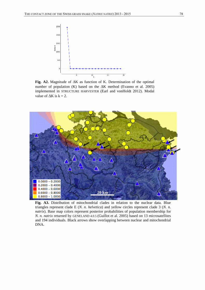
THE CONTACT ZONE OF THE SWISS GRASS SNAKE (NATRIX NATRIX) 2013 - 2015 78
Fig. A2. Magnitude of ∆K as function of K. Determination of the optimal
number of population (K) based on the ∆K method (Evanno et al. 2005)
implemented in STRUCTURE HARVESTER (Earl and vonHoldt 2012). Modal
value of ∆K is k = 2.
Fig. A3. Distribution of mitochondrial clades in relation to the nuclear data. Blue
triangles represent clade E (N. n. helvetica) and yellow circles represent clade 3 (N. n.
natrix). Base map colors represent posterior probabilities of population membership for
N. n. natrix returned by GENELAND 4.0.5 (Guillot et al. 2005) based on 13 microsatellites
and 194 individuals. Black arrows show overlapping between nuclear and mitochondrial
DNA.
20 km
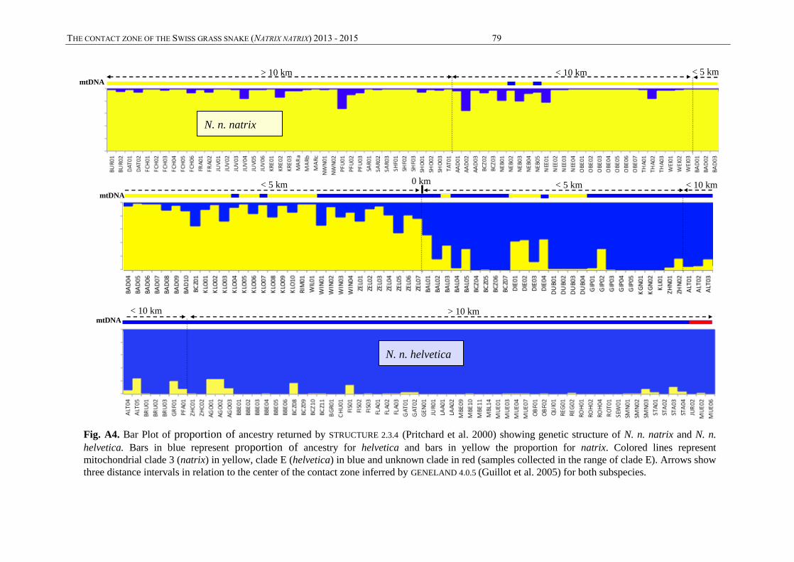
THE CONTACT ZONE OF THE SWISS GRASS SNAKE (NATRIX NATRIX) 2013 - 2015 79
mtDNA
> 10 km < 10 km < 5 km
< 5 km 0 km
mtDNA
mtDNA
< 5 km < 10 km
> 10 km < 10 km
Fig. A4. Bar Plot of proportion of ancestry returned by STRUCTURE 2.3.4 (Pritchard et al. 2000) showing genetic structure of N. n. natrix and N. n.
helvetica. Bars in blue represent proportion of ancestry for helvetica and bars in yellow the proportion for natrix. Colored lines represent
mitochondrial clade 3 (natrix) in yellow, clade E (helvetica) in blue and unknown clade in red (samples collected in the range of clade E). Arrows show
three distance intervals in relation to the center of the contact zone inferred by GENELAND 4.0.5 (Guillot et al. 2005) for both subspecies.
N. n. helvetica
N. n. natrix
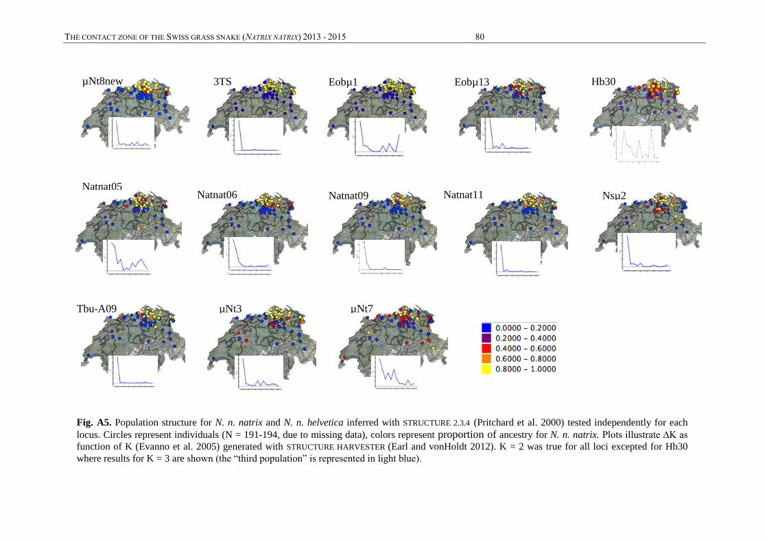
THE CONTACT ZONE OF THE SWISS GRASS SNAKE (NATRIX NATRIX) 2013 - 2015 80
µNt8new 3TS Eobµ13 Eobµ1 Hb30
Natnat05 Natnat06 Natnat09 Natnat11 Nsµ2
Tbu-A09 µNt3 µNt7
Fig. A5. Population structure for N. n. natrix and N. n. helvetica inferred with STRUCTURE 2.3.4 (Pritchard et al. 2000) tested independently for each
locus. Circles represent individuals (N = 191-194, due to missing data), colors represent proportion of ancestry for N. n. natrix. Plots illustrate ∆K as
function of K (Evanno et al. 2005) generated with STRUCTURE HARVESTER (Earl and vonHoldt 2012). K = 2 was true for all loci excepted for Hb30
where results for K = 3 are shown (the “third population” is represented in light blue).
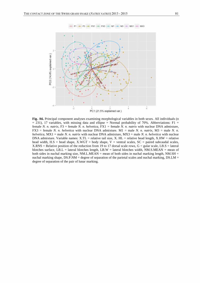
THE CONTACT ZONE OF THE SWISS GRASS SNAKE (NATRIX NATRIX) 2013 - 2015 81
Fig. A6. Principal component analyses examining morphological variables in both sexes. All individuals (n
= 231), 17 variables, with missing data and ellipse = Normal probability of 70%. Abbreviations: F1 =
female N. n. natrix, F3 = female N. n. helvetica, FX1 = female N. n. natrix with nuclear DNA admixture,
FX3 = female N. n. helvetica with nuclear DNA admixture. M1 = male N. n. natrix, M3 = male N. n.
helvetica, MX1 = male N. n. natrix with nuclear DNA admixture, MX3 = male N. n. helvetica with nuclear
DNA admixture. Variable names: X.TL = relative tail size, X. HL = relative head length, X.HW = relative
head width, H.S = head shape, X.WGT = body shape, V = ventral scales, SC = paired subcaudal scales,
X.RNS = Relative position of the reduction from 19 to 17 dorsal scale rows, G = gular scale, LB.S = lateral
blotches surface, LB.L = lateral blotches length, LB.W = lateral blotches width, NM.S.MEAN = mean of
both sides in nuchal marking size, NM.L.MEAN = mean of both sides in nuchal marking length, NM.SH =
nuchal marking shape, DS.P.NM = degree of separation of the parietal scales and nuchal marking, DS.LM =
degree of separation of the pair of lunar marking.

THE CONTACT ZONE OF THE SWISS GRASS SNAKE (NATRIX NATRIX) 2013 - 2015 82
Fig. A7. Principal component analyses examining morphological variables in females with putative hybrids.
(A.) Females (n = 139), 17 variables, with missing data, ellipse = Normal probability of 80%. (B.) Females (n
=139), 11 variables, with missing data, ellipse = Normal probability of 80%. Abbreviations: F1 = female N. n.
natrix, F3 = female N. n. helvetica, FX1 = female N. n. natrix with nuclear DNA admixture, FX3 = female N.
n. helvetica with nuclear DNA admixture. Variable names: X.TL = relative tail size, X. HL = relative head
length, X.HW = relative head width, H.S = head shape, X.WGT = body shape, V = ventral scales, SC = paired
subcaudal scales, X.RNS = Relative position of the reduction from 19 to 17 dorsal scale rows, G = gular scale,
LB.S = lateral blotches surface, LB.L = lateral blotches length, LB.W = lateral blotches width, NM.S.MEAN =
mean of both sides in nuchal marking size, NM.L.MEAN = mean of both sides in nuchal marking length,
NM.SH = nuchal marking shape, DS.P.NM = degree of separation of the parietal scales and nuchal marking,
DS.LM = degree of separation of the pair of lunar marking.
A. B.
Fig. A8. Morphology in females (PC1 scores) in relation to genetic data (microsatellites).
Females (n = 139), 11 morphological variables, with missing data and with putative hybrids.
PC1 scores come from the PCA showed in figure A7 (B.). Circles represent individuals and
colors referred to PC1 scores (values divided by quantiles). The base colors of the map indicate
a higher probability to belong either to N. n. natrix (yellow) or N. n. helvetica (blue), based on
microsatellite data calculated with GENELAND 4.0.5 (Guillot et al. 2005).
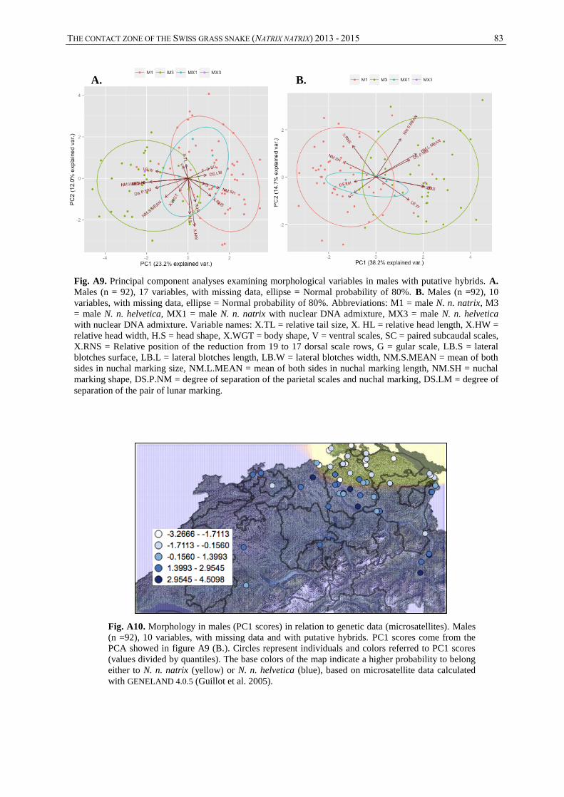
THE CONTACT ZONE OF THE SWISS GRASS SNAKE (NATRIX NATRIX) 2013 - 2015 83
Fig. A9. Principal component analyses examining morphological variables in males with putative hybrids. A.
Males (n = 92), 17 variables, with missing data, ellipse = Normal probability of 80%. B. Males (n =92), 10
variables, with missing data, ellipse = Normal probability of 80%. Abbreviations: M1 = male N. n. natrix, M3
= male N. n. helvetica, MX1 = male N. n. natrix with nuclear DNA admixture, MX3 = male N. n. helvetica
with nuclear DNA admixture. Variable names: X.TL = relative tail size, X. HL = relative head length, X.HW =
relative head width, H.S = head shape, X.WGT = body shape, V = ventral scales, SC = paired subcaudal scales,
X.RNS = Relative position of the reduction from 19 to 17 dorsal scale rows, G = gular scale, LB.S = lateral
blotches surface, LB.L = lateral blotches length, LB.W = lateral blotches width, NM.S.MEAN = mean of both
sides in nuchal marking size, NM.L.MEAN = mean of both sides in nuchal marking length, NM.SH = nuchal
marking shape, DS.P.NM = degree of separation of the parietal scales and nuchal marking, DS.LM = degree of
separation of the pair of lunar marking.
Fig. A10. Morphology in males (PC1 scores) in relation to genetic data (microsatellites). Males
(n =92), 10 variables, with missing data and with putative hybrids. PC1 scores come from the
PCA showed in figure A9 (B.). Circles represent individuals and colors referred to PC1 scores
(values divided by quantiles). The base colors of the map indicate a higher probability to belong
either to N. n. natrix (yellow) or N. n. helvetica (blue), based on microsatellite data calculated
with GENELAND 4.0.5 (Guillot et al. 2005).
A. B.
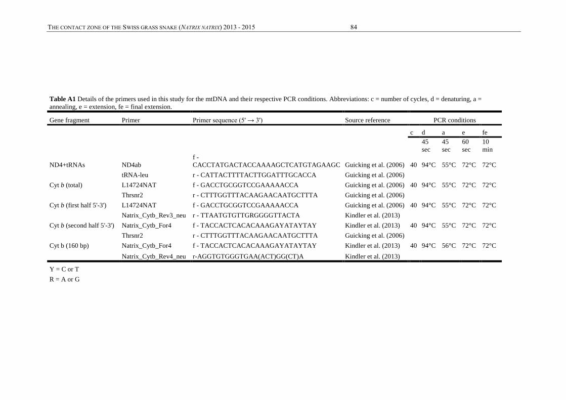
THE CONTACT ZONE OF THE SWISS GRASS SNAKE (NATRIX NATRIX) 2013 - 2015 84
Table A1 Details of the primers used in this study for the mtDNA and their respective PCR conditions. Abbreviations: c = number of cycles, d = denaturing, a =
annealing, e = extension, fe = final extension.
Gene fragment Primer Primer sequence (5' → 3') Source reference PCR conditions
c d a e fe
45
sec
45
sec
60
sec
10
min
ND4+tRNAs ND4ab
f -
CACCTATGACTACCAAAAGCTCATGTAGAAGC Guicking et al. (2006) 40 94°C 55°C 72°C 72°C
tRNA-leu r - CATTACTTTTACTTGGATTTGCACCA Guicking et al. (2006)
Cyt b (total) L14724NAT f - GACCTGCGGTCCGAAAAACCA Guicking et al. (2006) 40 94°C 55°C 72°C 72°C
Thrsnr2 r - CTTTGGTTTACAAGAACAATGCTTTA Guicking et al. (2006)
Cyt b (first half 5'-3') L14724NAT f - GACCTGCGGTCCGAAAAACCA Guicking et al. (2006) 40 94°C 55°C 72°C 72°C
Natrix_Cytb_Rev3_neu r - TTAATGTGTTGRGGGGTTACTA Kindler et al. (2013)
Cyt b (second half 5'-3') Natrix_Cytb_For4 f - TACCACTCACACAAAGAYATAYTAY Kindler et al. (2013) 40 94°C 55°C 72°C 72°C
Thrsnr2 r - CTTTGGTTTACAAGAACAATGCTTTA Guicking et al. (2006)
Cyt b (160 bp) Natrix_Cytb_For4 f - TACCACTCACACAAAGAYATAYTAY Kindler et al. (2013) 40 94°C 56°C 72°C 72°C
Natrix_Cytb_Rev4_neu r-AGGTGTGGGTGAA(ACT)GG(CT)A Kindler et al. (2013)
Y = C or T
R = A or G
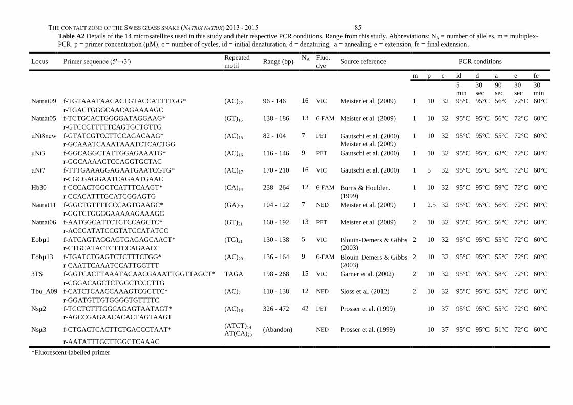
THE CONTACT ZONE OF THE SWISS GRASS SNAKE (NATRIX NATRIX) 2013 - 2015 85
Table A2 Details of the 14 microsatellites used in this study and their respective PCR conditions. Range from this study. Abbreviations: NA = number of alleles, m = multiplex-
PCR, p = primer concentration (µM), c = number of cycles, id = initial denaturation, d = denaturing, a = annealing, e = extension, fe = final extension.
Locus Primer sequence (5'→3') Repeated
motif Range (bp)
NA Fluo.
dye Source reference PCR conditions
m p c id d a e fe
5
min
30
sec
90
sec
30
sec
30
min
Natnat09 f-TGTAAATAACACTGTACCATTTTGG* (AC)22 96 - 146 16 VIC Meister et al. (2009) 1 10 32 95°C 95°C 56°C 72°C 60°C
r-TGACTGGGCAACAGAAAAGC
Natnat05 f-TCTGCACTGGGGATAGGAAG* (GT)16 138 - 186 13 6-FAM Meister et al. (2009) 1 10 32 95°C 95°C 56°C 72°C 60°C
r-GTCCCTTTTTCAGTGCTGTTG
μNt8new f-GTATCGTCCTTCCAGACAAG* (AC)15 82 - 104 7 PET Gautschi et al. (2000),
Meister et al. (2009)
1 10 32 95°C 95°C 55°C 72°C 60°C
r-GCAAATCAAATAAATCTCACTGG
μNt3 f-GGCAGGCTATTGGAGAAATG* (AC)16 116 - 146 9 PET Gautschi et al. (2000) 1 10 32 95°C 95°C 63°C 72°C 60°C
r-GGCAAAACTCCAGGTGCTAC
μNt7 f-TTTGAAAGGAGAATGAATCGTG* (AC)17 170 - 210 16 VIC Gautschi et al. (2000) 1 5 32 95°C 95°C 58°C 72°C 60°C
r-CGCGAGGAATCAGAATGAAC
Hb30 f-CCCACTGGCTCATTTCAAGT* (CA)14 238 - 264 12 6-FAM Burns & Houlden.
(1999)
1 10 32 95°C 95°C 59°C 72°C 60°C
r-CCACATTTGCATCGGAGTG
Natnat11 f-GGCTGTTTTCCCAGTGAAGC* (GA)13 104 - 122 7 NED Meister et al. (2009) 1 2.5 32 95°C 95°C 56°C 72°C 60°C
r-GGTCTGGGGAAAAAGAAAGG
Natnat06 f-AATGGCATTCTCTCCAGCTC* (GT)21 160 - 192 13 PET Meister et al. (2009) 2 10 32 95°C 95°C 56°C 72°C 60°C
r-ACCCATATCCGTATCCATATCC
Eobµ1 f-ATCAGTAGGAGTGAGAGCAACT* (TG)21 130 - 138 5 VIC Blouin-Demers & Gibbs
(2003)
2 10 32 95°C 95°C 55°C 72°C 60°C
r-CTGCATACTCTTCCAGAACC
Eobµ13 f-TGATCTGAGTCTCTTTCTGG* (AC)20 136 - 164 9 6-FAM Blouin-Demers & Gibbs
(2003)
2 10 32 95°C 95°C 55°C 72°C 60°C
r-CAATTCAAATCCATTGGTTT
3TS f-GGTCACTTAAATACAACGAAATTGGTTAGCT* TAGA 198 - 268 15 VIC Garner et al. (2002) 2 10 32 95°C 95°C 58°C 72°C 60°C
r-CGGACAGCTCTGGCTCCCTTG
Tbu_A09 f-CATCTCAACCAAAGTCGCTTC* (AC)7 110 - 138 12 NED Sloss et al. (2012) 2 10 32 95°C 95°C 55°C 72°C 60°C
r-GGATGTTGTGGGGTGTTTTC
Nsµ2 f-TCCTCTTTGGCAGAGTAATAGT* (AC)18 326 - 472 42 PET Prosser et al. (1999)
10 37 95°C 95°C 55°C 72°C 60°C
r-AGCCGAGAACACACTAGTAAGT
Nsµ3 f-CTGACTCACTTCTGACCCTAAT* (ATCT)14
AT(CA)20 (Abandon)
NED Prosser et al. (1999)
10 37 95°C 95°C 51°C 72°C 60°C
r-AATATTTGCTTGGCTCAAAC
*Fluorescent-labelled primer
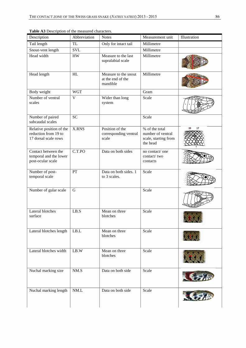
THE CONTACT ZONE OF THE SWISS GRASS SNAKE (NATRIX NATRIX) 2013 - 2015 86
Table A3 Description of the measured characters.
Description Abbreviation Notes Measurement unit Illustration
Tail length TL Only for intact tail Millimetre
Snout-vent length SVL Millimetre
Head width HW Measure to the last
supralabial scale
Millimetre
Head length HL Measure to the snout
at the end of the
mandible
Millimetre
Body weight WGT Gram
Number of ventral
scales
V Wider than long
system
Scale
Number of paired
subcaudal scales
SC Scale
Relative position of the
reduction from 19 to
17 dorsal scale rows
X.RNS Position of the
corresponding ventral
scale
% of the total
number of ventral
scale, starting from
the head
Contact between the
temporal and the lower
post-ocular scale
C.T.PO Data on both sides no contact/ one
contact/ two
contacts
Number of post-
temporal scale
PT Data on both sides. 1
to 3 scales.
Scale
Number of gular scale G Scale
Lateral blotches
surface
LB.S Mean on three
blotches
Scale
Lateral blotches length LB.L Mean on three
blotches
Scale
Lateral blotches width LB.W Mean on three
blotches
Scale
Nuchal marking size NM.S Data on both side Scale
Nuchal marking length NM.L Data on both side Scale
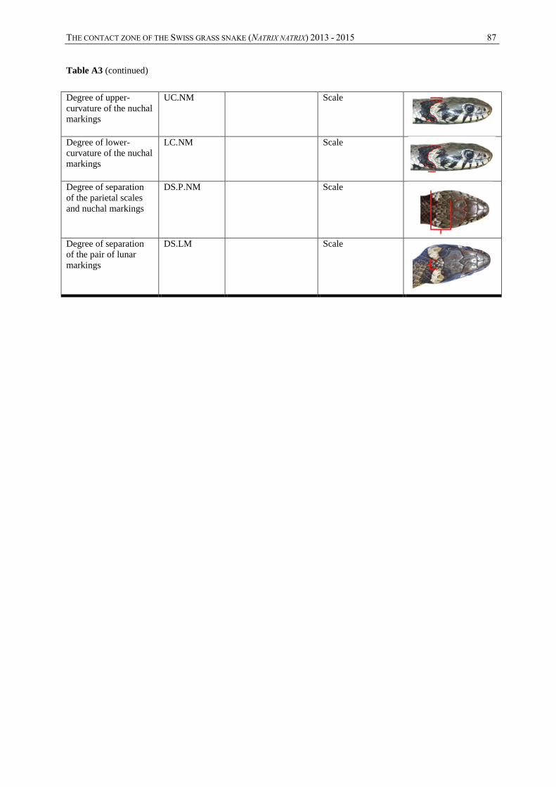
THE CONTACT ZONE OF THE SWISS GRASS SNAKE (NATRIX NATRIX) 2013 - 2015 87
Table A3 (continued)
Degree of upper-
curvature of the nuchal
markings
UC.NM Scale
Degree of lower-
curvature of the nuchal
markings
LC.NM Scale
Degree of separation
of the parietal scales
and nuchal markings
DS.P.NM Scale
Degree of separation
of the pair of lunar
markings
DS.LM Scale

THE CONTACT ZONE OF THE SWISS GRASS SNAKE (NATRIX NATRIX) 2013 - 2015 88
Table A4. Univariate morphological comparison for female N. natrix. N = number of individuals. Variables names: TOT.L = total length, X.TL = relative tail size, X.HL
= relative head length, X.HW = relative head width, HS = head shape, X.WGT = body shape, V = ventral scales, SC = paired subcaudal scales, X.RNS = relative position
of the reduction from 19 to 17 dorsal scale rows, C.T.PO = contact temporal scale-postoccular inferior scale, PT.MAX = maximum number of post-temporal scale, G =
gular scale, LB.S = lateral blotches size, LB.L = lateral blotches length, LB.W = lateral blotches width, NM.S.MEAN = mean of both sides in nuchal marking size,
NM.L.MEAN = mean of both sides in nuchal marking length, NM.SH = nuchal marking shape, DS.P.NM = degree of separation of the parietal scales and nuchal
marking, DS.LM = degree of separation of the pair of lunar marking.
Variables Test P-value Statistic Subspecies N Mean +/- SE Minima ; maxima Unit
Correction for
normality
TOT.L ANOVA 0.9581 F1, 118 = 0.0028 natrix 52 859 ± 192 311 ; 1214 mm
helvetica 68 866 ± 167 394 ; 1145
X.TL ANOVA 0.1434 F1, 101 = 2.175 natrix 43 0.179 ± 0.014 0.142 ; 0.207 mm/mm
helvetica 60 0.183 ± 0.011 0.144 ; 0.202
X.HL ANOVA 0.000643 *** F1, 113 = 12.33 natrix 50 0.043 ± 0.003 0.039 ; 0.049 mm/mm
helvetica 65 0.045 ± 0.003 0.039 ;0.055
X.HW ANOVA <0.0001*** F1, 113 = 18.3 natrix 50 0.025 ± 0.002 0.02 ; 0.03 mm/mm ln(x)
helvetica 65 0.027 ± 0.003 0.02 ; 0.036
HS ANOVA 0.0084 ** F1, 113 = 7.197 natrix 50 0.569 ± 0.038 0.471 ; 0.646 mm/mm ln(x)
helvetica 65 0.592 ± 0.051 0.472 ; 0.709
X.WGT ANOVA 0.873 F1, 58 = 0.02561 natrix 35 0.247 ± 0.108 0.074 ; 0.533 g/mm
helvetica 25 0.252 ± 0.121 0.089 ; 0.513
V ANOVA 0.9519 F1, 117 = 0.00366 natrix 52 170.64 ± 4.215 164 ; 182 scale
helvetica 67 170.69 ± 3.418 163 ; 179
SC ANOVA 0.2944 F1, 102 = 1.11 natrix 42 56.821 ± 4.124 46 ; 64 scale
helvetica 62 57.6290 ± 3.627 49 ; 67.5
X.RNS ANOVA <0.0001*** F1, 114 = 42.34 natrix 49 57.781 ± 7.601 52.601 ; 67.630 scale/scale
helvetica 67 53.514 ± 7.315 41.667 ; 63.636
C.T.PO Chi-square 0.000103*** χ22 = 18.3617 natrix 51 ratio = 36 : 8 : 7 - 2, 1 or 0
contacts helvetica 67 ratio = 21 : 19 : 27 -
PT.MAX Chi-square <0.0001*** χ22 = 22.729 natrix 52 ratio = 2 : 41 : 9 - 1, 2 or 3
scales helvetica 67 ratio = 3 : 24 : 40 -

THE CONTACT ZONE OF THE SWISS GRASS SNAKE (NATRIX NATRIX) 2013 - 2015 89
Table A4. (Continued) Univariate morphological comparison for female N. natrix. N = number of individuals. Variables names: TOT.L = total length, X.TL = relative tail
size, X.HL = relative head length, X.HW = relative head width, HS = head shape, X.WGT = body shape, V = ventral scales, SC = paired subcaudal scales, X.RNS =
relative position of the reduction from 19 to 17 dorsal scale rows, C.T.PO = contact temporal scale-postoccular inferior scale, PT.MAX = maximum number of post-
temporal scale, G = gular scale, LB.S = lateral blotches size, LB.L = lateral blotches length, LB.W = lateral blotches width, NM.S.MEAN = mean of both sides in nuchal
marking size, NM.L.MEAN = mean of both sides in nuchal marking length, NM.SH = nuchal marking shape, DS.P.NM = degree of separation of the parietal scales and
nuchal marking, DS.LM = degree of separation of the pair of lunar marking.
Variables Test P-value Statistic Subspecies N Mean +/- SE Minima ; maxima Unit
Correction for
normality
G Wilcoxon 0.000508*** W = 2313.5 natrix 52 10.538 ± 2.638 6 ; 18 scales
non-parametric helvetica 65 9.062 ± 2.022 5 ; 17
LB.S t-test (Welch) <0.0001*** t92.49 = -12.264 natrix 52 0.565 ± 0.309 0.12 ; 1.5 scales ln(x)
helvetica 58 1.677 ± 0.675 0.6 ; 4.5
LB.L t-test (Welch) <0.0001*** t96.60 = -11.4577 natrix 52 1.326 ± 0.64 0.4 ; 2.9 scales
helvetica 57 3.143 ± 0.993 1 ; 5.17
LB.W ANOVA 0.000193 *** F1, 107 = 14.91 natrix 52 0.529 ± 0.193 0.2 ; 1.17 scales ln(x)
helvetica 57 0.675 ± 0.211 0.28 ; 1.2
NM.S.MEAN ANOVA <0.0001*** F1, 105 = 18.53 natrix 49 19.967 ± 5.299 8 ; 35.75 scales
helvetica 58 24.198 ± 4.859 14 ; 36.5
NM.L.MEAN ANOVA <0.0001*** F1, 106 = 82.11 natrix 50 2.954 ± 0.581 1.55 ; 5.4 scales
helvetica 58 3.909 ± 0.514 2.75 ; 5.2
NM.SH ANOVA <0.0001*** F1, 107 = 50.76 natrix 50 1.477 ± 0.553 0.543 ; 2.667 scales ln(x)
helvetica 59 0.866 ± 0.323 0.314 ; 1.778
DS.P.NM ANOVA <0.0001*** F1, 107 = 50.16 natrix 50 2.959 ± 0.436 2.2 ; 4 scales
helvetica 59 3.638 ± 0.546 2.5 ; 5
DS.LM ANOVA 0.487 F1, 88 = 0.487 natrix 50 3.824 ± 1.806 0 ; 7 scales
helvetica 40 3.563 ± 1.714 0 ; 8
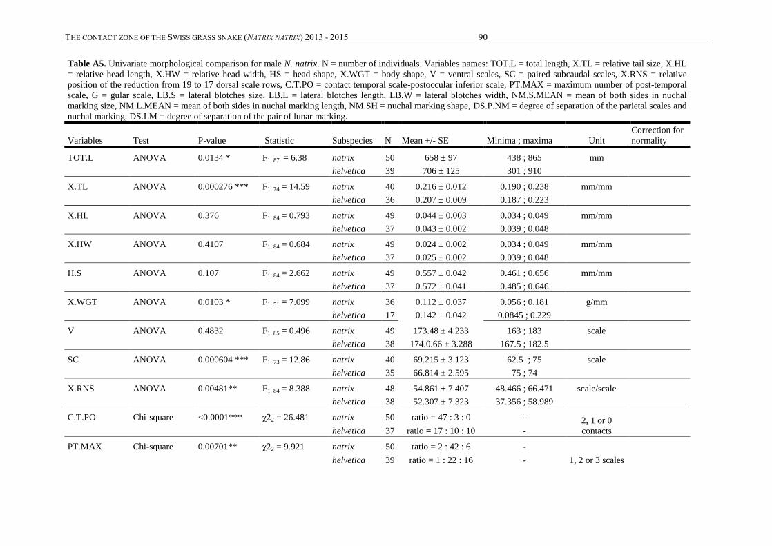
THE CONTACT ZONE OF THE SWISS GRASS SNAKE (NATRIX NATRIX) 2013 - 2015 90
Table A5. Univariate morphological comparison for male N. natrix. N = number of individuals. Variables names: TOT.L = total length, X.TL = relative tail size, X.HL
= relative head length, X.HW = relative head width, HS = head shape, X.WGT = body shape, V = ventral scales, SC = paired subcaudal scales, X.RNS = relative
position of the reduction from 19 to 17 dorsal scale rows, C.T.PO = contact temporal scale-postoccular inferior scale, PT.MAX = maximum number of post-temporal
scale, G = gular scale, LB.S = lateral blotches size, LB.L = lateral blotches length, LB.W = lateral blotches width, NM.S.MEAN = mean of both sides in nuchal
marking size, NM.L.MEAN = mean of both sides in nuchal marking length, NM.SH = nuchal marking shape, DS.P.NM = degree of separation of the parietal scales and
nuchal marking, DS.LM = degree of separation of the pair of lunar marking.
Variables Test P-value Statistic Subspecies N Mean +/- SE Minima ; maxima Unit
Correction for
normality
TOT.L ANOVA 0.0134 * F1, 87 = 6.38 natrix 50 658 ± 97 438 ; 865 mm
helvetica 39 706 ± 125 301 ; 910
X.TL ANOVA 0.000276 *** F1, 74 = 14.59 natrix 40 0.216 ± 0.012 0.190 ; 0.238 mm/mm
helvetica 36 0.207 ± 0.009 0.187 ; 0.223
X.HL ANOVA 0.376 F1, 84 = 0.793 natrix 49 0.044 ± 0.003 0.034 ; 0.049 mm/mm
helvetica 37 0.043 ± 0.002 0.039 ; 0.048
X.HW ANOVA 0.4107 F1, 84 = 0.684 natrix 49 0.024 ± 0.002 0.034 ; 0.049 mm/mm
helvetica 37 0.025 ± 0.002 0.039 ; 0.048
H.S ANOVA 0.107 F1, 84 = 2.662 natrix 49 0.557 ± 0.042 0.461 ; 0.656 mm/mm
helvetica 37 0.572 ± 0.041 0.485 ; 0.646
X.WGT ANOVA 0.0103 * F1, 51 = 7.099 natrix 36 0.112 ± 0.037 0.056 ; 0.181 g/mm
helvetica 17 0.142 ± 0.042 0.0845 ; 0.229
V ANOVA 0.4832 F1, 85 = 0.496 natrix 49 173.48 ± 4.233 163 ; 183 scale
helvetica 38 174.0.66 ± 3.288 167.5 ; 182.5
SC ANOVA 0.000604 *** F1, 73 = 12.86 natrix 40 69.215 ± 3.123 62.5 ; 75 scale
helvetica 35 66.814 ± 2.595 75 ; 74
X.RNS ANOVA 0.00481** F1, 84 = 8.388 natrix 48 54.861 ± 7.407 48.466 ; 66.471 scale/scale
helvetica 38 52.307 ± 7.323 37.356 ; 58.989
C.T.PO Chi-square <0.0001*** χ22 = 26.481 natrix 50 ratio = 47 : 3 : 0 - 2, 1 or 0
contacts helvetica 37 ratio = 17 : 10 : 10 -
PT.MAX Chi-square 0.00701** χ22 = 9.921 natrix 50 ratio = 2 : 42 : 6 -
1, 2 or 3 scales helvetica 39 ratio = 1 : 22 : 16 -
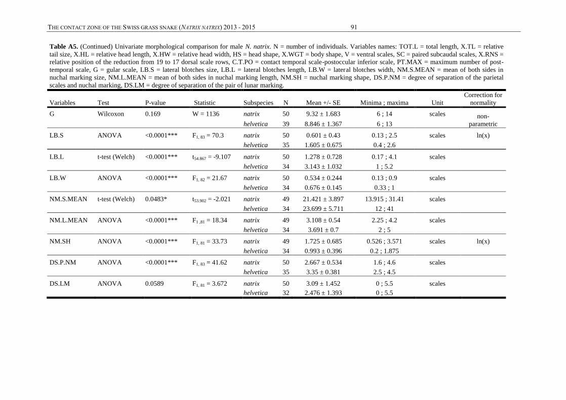
THE CONTACT ZONE OF THE SWISS GRASS SNAKE (NATRIX NATRIX) 2013 - 2015 91
Table A5. (Continued) Univariate morphological comparison for male N. natrix. N = number of individuals. Variables names: TOT.L = total length, X.TL = relative
tail size, X.HL = relative head length, X.HW = relative head width, HS = head shape, X.WGT = body shape, V = ventral scales, SC = paired subcaudal scales, X.RNS =
relative position of the reduction from 19 to 17 dorsal scale rows, C.T.PO = contact temporal scale-postoccular inferior scale, PT.MAX = maximum number of post-
temporal scale, G = gular scale, LB.S = lateral blotches size, LB.L = lateral blotches length, LB.W = lateral blotches width, NM.S.MEAN = mean of both sides in
nuchal marking size, NM.L.MEAN = mean of both sides in nuchal marking length, NM.SH = nuchal marking shape, DS.P.NM = degree of separation of the parietal
scales and nuchal marking, DS.LM = degree of separation of the pair of lunar marking.
Variables Test P-value Statistic Subspecies N Mean +/- SE Minima ; maxima Unit
Correction for
normality
G Wilcoxon 0.169 W = 1136 natrix 50 9.32 ± 1.683 6 ; 14 scales non-
parametric helvetica 39 8.846 ± 1.367 6 ; 13
LB.S ANOVA <0.0001*** F1, 83 = 70.3 natrix 50 0.601 ± 0.43 0.13 ; 2.5 scales ln(x)
helvetica 35 1.605 ± 0.675 0.4 ; 2.6
LB.L t-test (Welch) <0.0001*** t54.867 = -9.107 natrix 50 1.278 ± 0.728 0.17 ; 4.1 scales
helvetica 34 3.143 ± 1.032 1 ; 5.2
LB.W ANOVA <0.0001*** F1, 82 = 21.67 natrix 50 0.534 ± 0.244 0.13 ; 0.9 scales
helvetica 34 0.676 ± 0.145 0.33 ; 1
NM.S.MEAN t-test (Welch) 0.0483* t53.902 = -2.021 natrix 49 21.421 ± 3.897 13.915 ; 31.41 scales
helvetica 34 23.699 ± 5.711 12 ; 41
NM.L.MEAN ANOVA <0.0001*** F1 ,81 = 18.34 natrix 49 3.108 ± 0.54 2.25 ; 4.2 scales
helvetica 34 3.691 ± 0.7 2 ; 5
NM.SH ANOVA <0.0001*** F1, 81 = 33.73 natrix 49 1.725 ± 0.685 0.526 ; 3.571 scales ln(x)
helvetica 34 0.993 ± 0.396 0.2 ; 1.875
DS.P.NM ANOVA <0.0001*** F1, 83 = 41.62 natrix 50 2.667 ± 0.534 1.6 ; 4.6 scales
helvetica 35 3.35 ± 0.381 2.5 ; 4.5
DS.LM ANOVA 0.0589 F1, 81 = 3.672 natrix 50 3.09 ± 1.452 0 ; 5.5 scales
helvetica 32 2.476 ± 1.393 0 ; 5.5
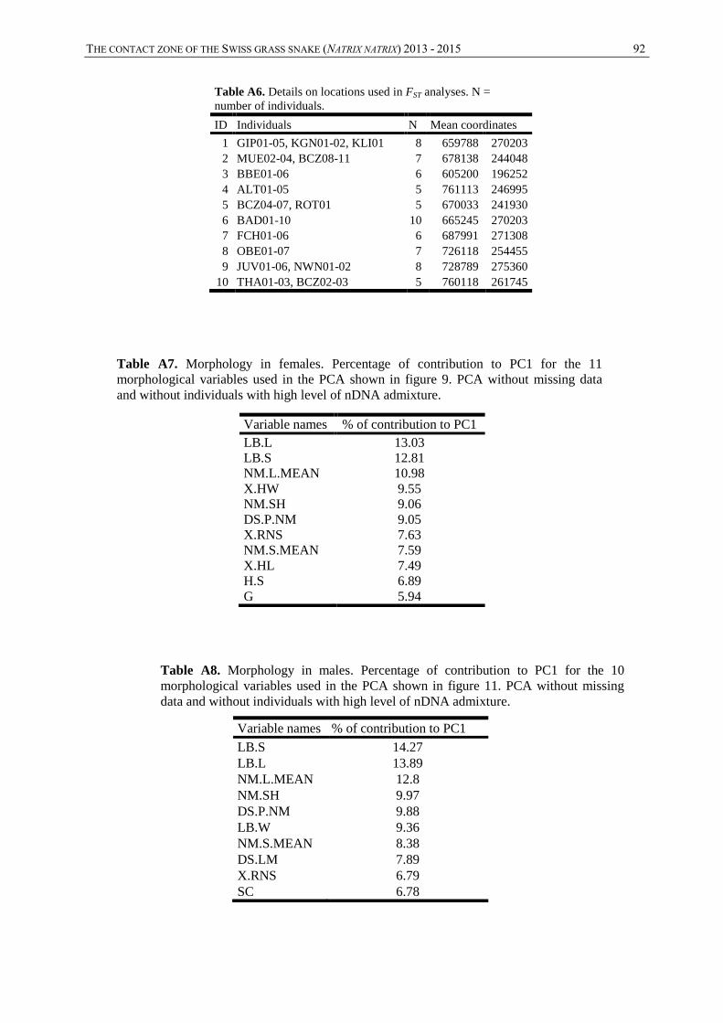
THE CONTACT ZONE OF THE SWISS GRASS SNAKE (NATRIX NATRIX) 2013 - 2015 92
Table A6. Details on locations used in FST analyses. N =
number of individuals.
ID Individuals N Mean coordinates
1 GIP01-05, KGN01-02, KLI01 8 659788 270203
2 MUE02-04, BCZ08-11 7 678138 244048
3 BBE01-06 6 605200 196252
4 ALT01-05 5 761113 246995
5 BCZ04-07, ROT01 5 670033 241930
6 BAD01-10 10 665245 270203
7 FCH01-06 6 687991 271308
8 OBE01-07 7 726118 254455
9 JUV01-06, NWN01-02 8 728789 275360
10 THA01-03, BCZ02-03 5 760118 261745
Variable names % of contribution to PC1
LB.L 13.03
LB.S 12.81
NM.L.MEAN 10.98
X.HW 9.55
NM.SH 9.06
DS.P.NM 9.05
X.RNS 7.63
NM.S.MEAN 7.59
X.HL 7.49
H.S 6.89
G 5.94
Variable names % of contribution to PC1
LB.S 14.27
LB.L 13.89
NM.L.MEAN 12.8
NM.SH 9.97
DS.P.NM 9.88
LB.W 9.36
NM.S.MEAN 8.38
DS.LM 7.89
X.RNS 6.79
SC 6.78
Table A7. Morphology in females. Percentage of contribution to PC1 for the 11
morphological variables used in the PCA shown in figure 9. PCA without missing data
and without individuals with high level of nDNA admixture.
Table A8. Morphology in males. Percentage of contribution to PC1 for the 10
morphological variables used in the PCA shown in figure 11. PCA without missing
data and without individuals with high level of nDNA admixture.
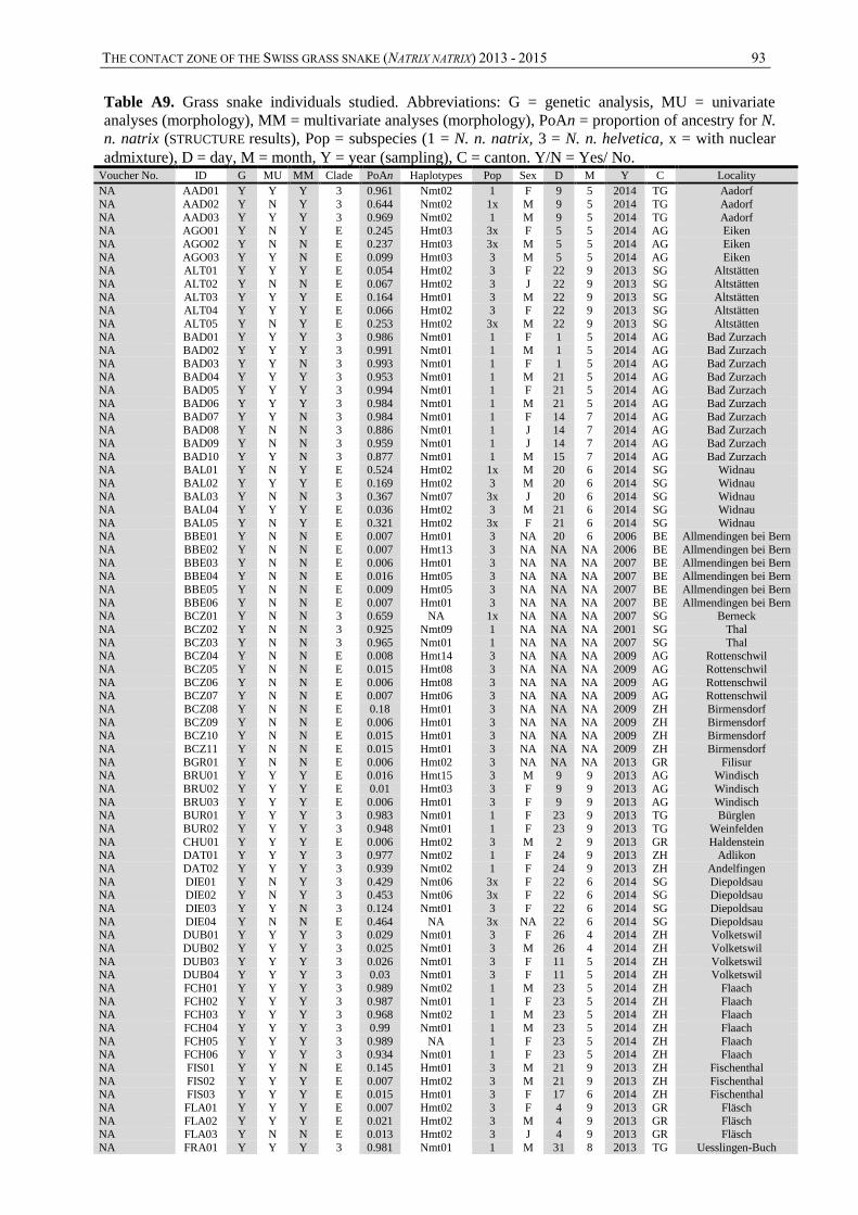
THE CONTACT ZONE OF THE SWISS GRASS SNAKE (NATRIX NATRIX) 2013 - 2015 93
Voucher No. ID G MU MM Clade PoAn Haplotypes Pop Sex D M Y C Locality
NA AAD01 Y Y Y 3 0.961 Nmt02 1 F 9 5 2014 TG Aadorf
NA AAD02 Y N Y 3 0.644 Nmt02 1x M 9 5 2014 TG Aadorf
NA AAD03 Y Y Y 3 0.969 Nmt02 1 M 9 5 2014 TG Aadorf NA AGO01 Y N Y E 0.245 Hmt03 3x F 5 5 2014 AG Eiken
NA AGO02 Y N N E 0.237 Hmt03 3x M 5 5 2014 AG Eiken
NA AGO03 Y Y N E 0.099 Hmt03 3 M 5 5 2014 AG Eiken NA ALT01 Y Y Y E 0.054 Hmt02 3 F 22 9 2013 SG Altstätten
NA ALT02 Y N N E 0.067 Hmt02 3 J 22 9 2013 SG Altstätten
NA ALT03 Y Y Y E 0.164 Hmt01 3 M 22 9 2013 SG Altstätten NA ALT04 Y Y Y E 0.066 Hmt02 3 F 22 9 2013 SG Altstätten
NA ALT05 Y N Y E 0.253 Hmt02 3x M 22 9 2013 SG Altstätten
NA BAD01 Y Y Y 3 0.986 Nmt01 1 F 1 5 2014 AG Bad Zurzach
NA BAD02 Y Y Y 3 0.991 Nmt01 1 M 1 5 2014 AG Bad Zurzach
NA BAD03 Y Y N 3 0.993 Nmt01 1 F 1 5 2014 AG Bad Zurzach
NA BAD04 Y Y Y 3 0.953 Nmt01 1 M 21 5 2014 AG Bad Zurzach NA BAD05 Y Y Y 3 0.994 Nmt01 1 F 21 5 2014 AG Bad Zurzach
NA BAD06 Y Y Y 3 0.984 Nmt01 1 M 21 5 2014 AG Bad Zurzach
NA BAD07 Y Y N 3 0.984 Nmt01 1 F 14 7 2014 AG Bad Zurzach NA BAD08 Y N N 3 0.886 Nmt01 1 J 14 7 2014 AG Bad Zurzach
NA BAD09 Y N N 3 0.959 Nmt01 1 J 14 7 2014 AG Bad Zurzach
NA BAD10 Y Y N 3 0.877 Nmt01 1 M 15 7 2014 AG Bad Zurzach NA BAL01 Y N Y E 0.524 Hmt02 1x M 20 6 2014 SG Widnau
NA BAL02 Y Y Y E 0.169 Hmt02 3 M 20 6 2014 SG Widnau
NA BAL03 Y N N 3 0.367 Nmt07 3x J 20 6 2014 SG Widnau NA BAL04 Y Y Y E 0.036 Hmt02 3 M 21 6 2014 SG Widnau
NA BAL05 Y N Y E 0.321 Hmt02 3x F 21 6 2014 SG Widnau NA BBE01 Y N N E 0.007 Hmt01 3 NA 20 6 2006 BE Allmendingen bei Bern
NA BBE02 Y N N E 0.007 Hmt13 3 NA NA NA 2006 BE Allmendingen bei Bern
NA BBE03 Y N N E 0.006 Hmt01 3 NA NA NA 2007 BE Allmendingen bei Bern
NA BBE04 Y N N E 0.016 Hmt05 3 NA NA NA 2007 BE Allmendingen bei Bern
NA BBE05 Y N N E 0.009 Hmt05 3 NA NA NA 2007 BE Allmendingen bei Bern
NA BBE06 Y N N E 0.007 Hmt01 3 NA NA NA 2007 BE Allmendingen bei Bern NA BCZ01 Y N N 3 0.659 NA 1x NA NA NA 2007 SG Berneck
NA BCZ02 Y N N 3 0.925 Nmt09 1 NA NA NA 2001 SG Thal
NA BCZ03 Y N N 3 0.965 Nmt01 1 NA NA NA 2007 SG Thal NA BCZ04 Y N N E 0.008 Hmt14 3 NA NA NA 2009 AG Rottenschwil
NA BCZ05 Y N N E 0.015 Hmt08 3 NA NA NA 2009 AG Rottenschwil
NA BCZ06 Y N N E 0.006 Hmt08 3 NA NA NA 2009 AG Rottenschwil NA BCZ07 Y N N E 0.007 Hmt06 3 NA NA NA 2009 AG Rottenschwil
NA BCZ08 Y N N E 0.18 Hmt01 3 NA NA NA 2009 ZH Birmensdorf
NA BCZ09 Y N N E 0.006 Hmt01 3 NA NA NA 2009 ZH Birmensdorf NA BCZ10 Y N N E 0.015 Hmt01 3 NA NA NA 2009 ZH Birmensdorf
NA BCZ11 Y N N E 0.015 Hmt01 3 NA NA NA 2009 ZH Birmensdorf
NA BGR01 Y N N E 0.006 Hmt02 3 NA NA NA 2013 GR Filisur NA BRU01 Y Y Y E 0.016 Hmt15 3 M 9 9 2013 AG Windisch
NA BRU02 Y Y Y E 0.01 Hmt03 3 F 9 9 2013 AG Windisch
NA BRU03 Y Y Y E 0.006 Hmt01 3 F 9 9 2013 AG Windisch
NA BUR01 Y Y Y 3 0.983 Nmt01 1 F 23 9 2013 TG Bürglen
NA BUR02 Y Y Y 3 0.948 Nmt01 1 F 23 9 2013 TG Weinfelden
NA CHU01 Y Y Y E 0.006 Hmt02 3 M 2 9 2013 GR Haldenstein NA DAT01 Y Y Y 3 0.977 Nmt02 1 F 24 9 2013 ZH Adlikon
NA DAT02 Y Y Y 3 0.939 Nmt02 1 F 24 9 2013 ZH Andelfingen
NA DIE01 Y N Y 3 0.429 Nmt06 3x F 22 6 2014 SG Diepoldsau NA DIE02 Y N Y 3 0.453 Nmt06 3x F 22 6 2014 SG Diepoldsau
NA DIE03 Y Y N 3 0.124 Nmt01 3 F 22 6 2014 SG Diepoldsau
NA DIE04 Y N N E 0.464 NA 3x NA 22 6 2014 SG Diepoldsau NA DUB01 Y Y Y 3 0.029 Nmt01 3 F 26 4 2014 ZH Volketswil
NA DUB02 Y Y Y 3 0.025 Nmt01 3 M 26 4 2014 ZH Volketswil
NA DUB03 Y Y Y 3 0.026 Nmt01 3 F 11 5 2014 ZH Volketswil NA DUB04 Y Y Y 3 0.03 Nmt01 3 F 11 5 2014 ZH Volketswil
NA FCH01 Y Y Y 3 0.989 Nmt02 1 M 23 5 2014 ZH Flaach
NA FCH02 Y Y Y 3 0.987 Nmt01 1 F 23 5 2014 ZH Flaach NA FCH03 Y Y Y 3 0.968 Nmt02 1 M 23 5 2014 ZH Flaach
NA FCH04 Y Y Y 3 0.99 Nmt01 1 M 23 5 2014 ZH Flaach
NA FCH05 Y Y Y 3 0.989 NA 1 F 23 5 2014 ZH Flaach
NA FCH06 Y Y Y 3 0.934 Nmt01 1 F 23 5 2014 ZH Flaach
NA FIS01 Y Y N E 0.145 Hmt01 3 M 21 9 2013 ZH Fischenthal
NA FIS02 Y Y Y E 0.007 Hmt02 3 M 21 9 2013 ZH Fischenthal NA FIS03 Y Y Y E 0.015 Hmt01 3 F 17 6 2014 ZH Fischenthal
NA FLA01 Y Y Y E 0.007 Hmt02 3 F 4 9 2013 GR Fläsch
NA FLA02 Y Y Y E 0.021 Hmt02 3 M 4 9 2013 GR Fläsch NA FLA03 Y N N E 0.013 Hmt02 3 J 4 9 2013 GR Fläsch
NA FRA01 Y Y Y 3 0.981 Nmt01 1 M 31 8 2013 TG Uesslingen-Buch
Table A9. Grass snake individuals studied. Abbreviations: G = genetic analysis, MU = univariate
analyses (morphology), MM = multivariate analyses (morphology), PoAn = proportion of ancestry for N.
n. natrix (STRUCTURE results), Pop = subspecies (1 = N. n. natrix, 3 = N. n. helvetica, x = with nuclear
admixture), D = day, M = month, Y = year (sampling), C = canton. Y/N = Yes/ No.
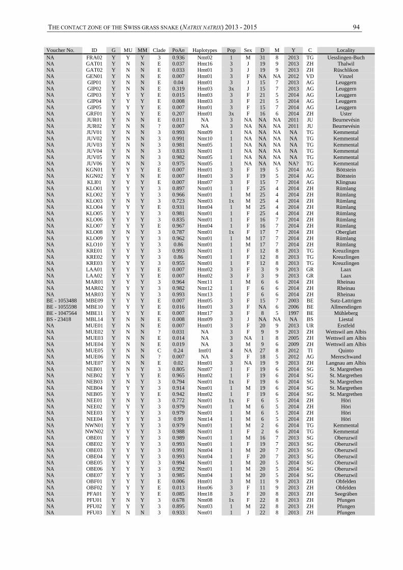
THE CONTACT ZONE OF THE SWISS GRASS SNAKE (NATRIX NATRIX) 2013 - 2015 94
Voucher No. ID G MU MM Clade PoAn Haplotypes Pop Sex D M Y C Locality
NA FRA02 Y Y Y 3 0.936 Nmt02 1 M 31 8 2013 TG Uesslingen-Buch NA GAT01 Y N N E 0.037 Hmt16 3 J 19 9 2013 ZH Thalwil
NA GAT02 Y N N E 0.033 Hmt01 3 J 19 9 2013 ZH Rüschlikon
NA GEN01 Y N N E 0.007 Hmt01 3 F NA NA 2012 VD Vinzel NA GIP01 Y N N E 0.04 Hmt01 3 J 15 7 2013 AG Leuggern
NA GIP02 Y N N E 0.319 Hmt03 3x J 15 7 2013 AG Leuggern
NA GIP03 Y Y Y E 0.015 Hmt03 3 F 21 5 2014 AG Leuggern NA GIP04 Y Y Y E 0.008 Hmt03 3 F 21 5 2014 AG Leuggern
NA GIP05 Y Y Y E 0.007 Hmt01 3 F 15 7 2014 AG Leuggern
NA GRF01 Y N Y E 0.207 Hmt01 3x F 16 6 2014 ZH Uster NA JUR01 Y N N E 0.011 NA 3 NA NA NA 2011 JU Beurnevésin
NA JUR02 Y N N ? 0.007 NA 3 NA NA NA 2011 JU Beurnevésin NA JUV01 Y N N 3 0.993 Nmt09 1 NA NA NA NA TG Kemmental
NA JUV02 Y N N 3 0.991 Nmt10 1 NA NA NA NA TG Kemmental
NA JUV03 Y N N 3 0.981 Nmt05 1 NA NA NA NA TG Kemmental NA JUV04 Y N N 3 0.833 Nmt01 1 NA NA NA NA TG Kemmental
NA JUV05 Y N N 3 0.982 Nmt05 1 NA NA NA NA TG Kemmental
NA JUV06 Y N N 3 0.975 Nmt05 1 NA NA NA NA? TG Kemmental NA KGN01 Y Y Y E 0.007 Hmt01 3 F 19 5 2014 AG Böttstein
NA KGN02 Y Y N E 0.007 Hmt01 3 F 19 5 2014 AG Böttstein
NA KLI01 Y Y Y E 0.007 Hmt07 3 F 15 7 2014 AG Klingnau NA KLO01 Y Y Y 3 0.897 Nmt01 1 F 25 4 2014 ZH Rümlang
NA KLO02 Y Y Y 3 0.966 Nmt01 1 M 25 4 2014 ZH Rümlang
NA KLO03 Y N Y 3 0.723 Nmt03 1x M 25 4 2014 ZH Rümlang NA KLO04 Y Y Y E 0.931 Hmt04 1 M 25 4 2014 ZH Rümlang
NA KLO05 Y Y Y 3 0.981 Nmt01 1 F 25 4 2014 ZH Rümlang
NA KLO06 Y Y Y 3 0.835 Nmt01 1 F 16 7 2014 ZH Rümlang NA KLO07 Y Y Y E 0.967 Hmt04 1 F 16 7 2014 ZH Rümlang
NA KLO08 Y N Y 3 0.787 Nmt01 1x F 17 7 2014 ZH Oberglatt
NA KLO09 Y Y Y 3 0.962 Nmt01 1 M 17 7 2014 ZH Rümlang NA KLO10 Y Y Y 3 0.86 Nmt01 1 M 17 7 2014 ZH Rümlang
NA KRE01 Y Y Y 3 0.993 Nmt01 1 F 12 8 2013 TG Kreuzlingen
NA KRE02 Y Y Y 3 0.86 Nmt01 1 F 12 8 2013 TG Kreuzlingen NA KRE03 Y Y Y 3 0.955 Nmt01 1 F 12 8 2013 TG Kreuzlingen
NA LAA01 Y Y Y E 0.007 Hmt02 3 F 3 9 2013 GR Laax
NA LAA02 Y Y Y E 0.007 Hmt02 3 F 3 9 2013 GR Laax NA MAR01 Y Y Y 3 0.964 Nmt11 1 M 6 6 2014 ZH Rheinau
NA MAR02 Y Y Y 3 0.982 Nmt12 1 F 6 6 2014 ZH Rheinau
NA MAR03 Y N Y 3 0.993 Nmt13 1 F 6 6 2014 ZH Rheinau BE - 1053488 MBE09 Y Y Y E 0.007 Hmt05 3 F 15 7 2003 BE Sutz-Lattrigen
BE - 1055598 MBE10 Y Y Y E 0.016 Hmt01 3 F NA 6 2006 BE Allmendingen
BE - 1047564 MBE11 Y Y Y E 0.007 Hmt17 3 F 8 5 1997 BE Mühleberg BS - 23418 MBL14 Y N N E 0.008 Hmt09 3 J NA NA NA BS Liestal
NA MUE01 Y N N E 0.007 Hmt01 3 F 20 9 2013 UR Erstfeld
NA MUE02 Y N N ? 0.031 NA 3 F 9 9 2013 ZH Wettswil am Albis NA MUE03 Y N N E 0.014 NA 3 NA 1 8 2005 ZH Wettswil am Albis
NA MUE04 Y N N E 0.019 NA 3 M 9 6 2009 ZH Wettswil am Albis
NA MUE05 Y N N C 0.24 Imt01 4 NA 27 8 2012 TI Quinto NA MUE06 Y N N ? 0.007 NA 3 F 18 5 2012 AG Mereschwand
NA MUE07 Y N N E 0.02 Hmt01 3 NA 19 9 2013 ZH Langnau am Albis
NA NEB01 Y N Y 3 0.805 Nmt07 1 F 19 6 2014 SG St. Margrethen NA NEB02 Y Y Y E 0.965 Hmt02 1 F 19 6 2014 SG St. Margrethen
NA NEB03 Y N Y 3 0.794 Nmt01 1x F 19 6 2014 SG St. Margrethen
NA NEB04 Y Y Y 3 0.914 Nmt01 1 M 19 6 2014 SG St. Margrethen NA NEB05 Y Y Y E 0.942 Hmt02 1 F 19 6 2014 SG St. Margrethen
NA NEE01 Y N Y 3 0.772 Nmt01 1x F 6 5 2014 ZH Höri
NA NEE02 Y Y Y 3 0.979 Nmt01 1 M 6 5 2014 ZH Höri NA NEE03 Y Y Y 3 0.979 Nmt01 1 M 6 5 2014 ZH Höri
NA NEE04 Y Y Y 3 0.99 Nmt14 1 M 6 5 2014 ZH Höri
NA NWN01 Y Y Y 3 0.979 Nmt01 1 M 2 6 2014 TG Kemmental NA NWN02 Y Y Y 3 0.988 Nmt01 1 F 2 6 2014 TG Kemmental
NA OBE01 Y Y Y 3 0.989 Nmt01 1 M 16 7 2013 SG Oberuzwil
NA OBE02 Y Y Y 3 0.993 Nmt01 1 F 19 7 2013 SG Oberuzwil NA OBE03 Y Y Y 3 0.991 Nmt04 1 M 20 7 2013 SG Oberuzwil
NA OBE04 Y Y Y 3 0.993 Nmt04 1 F 20 7 2013 SG Oberuzwil NA OBE05 Y Y Y 3 0.994 Nmt01 1 M 20 5 2014 SG Oberuzwil
NA OBE06 Y Y Y 3 0.992 Nmt01 1 M 20 5 2014 SG Oberuzwil
NA OBE07 Y Y Y 3 0.985 Nmt04 1 M 20 5 2014 SG Oberuzwil NA OBF01 Y Y Y E 0.006 Hmt01 3 M 11 9 2013 ZH Obfelden
NA OBF02 Y Y Y E 0.013 Hmt06 3 F 11 9 2013 ZH Obfelden
NA PFA01 Y Y Y E 0.085 Hmt18 3 F 20 8 2013 ZH Seegräben NA PFU01 Y N Y 3 0.678 Nmt08 1x F 22 8 2013 ZH Pfungen
NA PFU02 Y Y Y 3 0.895 Nmt03 1 M 22 8 2013 ZH Pfungen
NA PFU03 Y N N 3 0.933 Nmt01 1 J 22 8 2013 ZH Pfungen
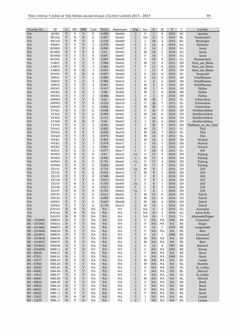
THE CONTACT ZONE OF THE SWISS GRASS SNAKE (NATRIX NATRIX) 2013 - 2015 95
Voucher No. ID G MU MM Clade PoAn Haplotypes Pop Sex D M Y C Locality
NA QUI01 Y Y Y E 0.009 Hmt04 3 F 1 8 2013 SG Quarten NA REG01 Y N N E 0.007 Hmt01 3 NA 25 4 2014 BL Frenkendorf
NA REG02 Y N N E 0.029 Hmt09 3 J 30 4 2014 BL Binningen
NA RIM01 Y Y Y 3 0.978 Nmt02 1 F 24 4 2014 AG Rietheim NA ROH01 Y Y Y E 0.006 Hmt07 3 F 16 5 2014 AG Aarau
NA ROH02 Y Y Y E 0.01 Hmt03 3 M 19 5 2014 AG Aarau
NA ROH04 Y Y Y E 0.007 Hmt07 3 F 18 7 2014 AG Aarau NA ROT01 Y Y Y E 0.007 Hmt06 3 F 10 8 2013 AG Rottenschwil
NA SAR01 Y Y Y 3 0.994 Nmt01 1 M 11 8 2013 SH Stein_am_Rhein
NA SAR02 Y Y Y 3 0.982 Nmt02 1 F 11 8 2013 SH Stein_am_Rhein NA SAR03 Y N N 3 0.993 Nmt03 1 J 11 8 2013 SH Stein_am_Rhein
NA SEW01 Y Y N E 0.007 Hmt02 3 F 23 6 2014 SG Sennwald NA SHF01 Y Y Y 3 0.989 Nmt01 1 F 25 9 2013 SH Schaffhausen
NA SHF02 Y Y Y 3 0.986 Nmt15 1 F 4 6 2014 SH Schaffhausen
NA SHF03 Y Y Y 3 0.991 Nmt01 1 M 4 6 2014 SH Schaffhausen NA SHO01 Y Y Y 3 0.937 Nmt01 1 M 5 6 2014 SH Hallau
NA SHO02 Y Y Y 3 0.98 Nmt01 1 M 5 6 2014 SH Hallau
NA SHO03 Y Y Y 3 0.968 Nmt01 1 F 5 6 2014 SH Hallau NA SMN01 Y Y Y E 0.02 Hmt10 3 M 30 7 2013 SG Schmerikon
NA SMN02 Y Y Y E 0.018 Hmt10 3 F 30 7 2013 SG Schmerikon
NA SMN03 Y Y Y E 0.084 Hmt11 3 M 30 7 2013 SG Schmerikon NA STA01 Y Y Y E 0.038 Hmt01 3 F 26 6 2014 ZH Hombrechtikon
NA STA02 Y Y Y E 0.009 Hmt01 3 M 26 6 2014 ZH Hombrechtikon
NA STA03 Y Y Y E 0.115 Hmt01 3 F 26 6 2014 ZH Hombrechtikon NA STA04 Y N N E 0.05 Hmt01 3 J 26 6 2014 ZH Hombrechtikon
NA TAT01 Y Y Y 3 0.991 Nmt03 1 F 30 8 2013 ZH Thalheim_an_der_Thur
NA THA01 Y Y Y 3 0.982 Nmt01 1 M 23 7 2013 SG Thal NA THA02 Y Y Y 3 0.839 Nmt16 1 M 26 7 2013 SG Thal
NA THA03 Y Y Y 3 0.973 Nmt01 1 M 14 8 2013 SG Thal
NA WEI01 Y Y Y 3 0.965 Nmt01 1 M 10 5 2014 ZH Weiach NA WEI02 Y Y Y 3 0.978 Nmt17 1 F 10 5 2014 ZH Weiach
NA WEI03 Y Y Y 3 0.991 Nmt08 1 F 10 5 2014 ZH Weiach
NA WIL01 Y Y Y 3 0.977 Nmt17 1 F 29 8 2013 SG Wil NA WIN01 Y N Y E 0.67 Hmt12 1x F 17 4 2014 ZH Kyburg
NA WIN02 Y Y Y E 0.942 Hmt01 1 M 17 4 2014 ZH Kyburg
NA WIN03 Y N Y E 0.791 Hmt01 1x F 17 4 2014 ZH Kyburg NA WIN04 Y Y Y E 0.854 Hmt01 1 M 17 4 2014 ZH Kyburg
NA ZEL01 Y N N E 0.731 Hmt01 1x M 8 5 2014 ZH Zell
NA ZEL02 Y Y Y E 0.912 Hmt12 1 M 8 5 2014 ZH Zell NA ZEL03 Y Y Y E 0.946 Hmt01 1 F 8 5 2014 ZH Zell
NA ZEL04 Y Y Y E 0.813 Hmt01 1 F 8 5 2014 ZH Zell
NA ZEL05 Y N Y E 0.556 Hmt01 1x F 8 5 2014 ZH Zell NA ZEL06 Y Y Y E 0.815 Hmt01 1 F 8 5 2014 ZH Zell
NA ZEL07 Y N Y E 0.763 Hmt01 1x F 8 5 2014 ZH Zell
NA ZHC01 Y Y Y E 0.012 Hmt01 3 M 25 6 2014 ZH Zürich NA ZHC02 Y Y Y E 0.009 Hmt01 3 M 25 6 2014 ZH Zürich
NA ZHN01 Y Y Y E 0.047 Hmt04 3 M 20 4 2014 ZH Zürich
NA ZHN02 Y Y Y E 0.178 Hmt11 3 M 16 5 2014 ZH Zürich NA BAG01 N N N NA NA NA 3 NA 6 4 2014 AG Auenstein
NA BAG02 N N N NA NA NA 3 NA 10 5 2014 AG Aarau Rohr
NA BAG03 N N N NA NA NA 1 NA 26 5 2014 TG Kleinandelfingen BE - 1016060 MBE01 N Y Y NA NA NA 3 F NA NA 1992 BE Utzenstorf
BE - 1015841 MBE02 N Y Y NA NA NA 3 F NA NA NA BE Ittigen
BE - 1015863 MBE03 N Y Y NA NA NA 3 F 16 5 1979 BE Längenbühl BE - 1016040 MBE04 N Y Y NA NA NA 3 F NA NA NA BE Bern
BE - 1016051 MBE05 N Y Y NA NA NA 3 F 23 7 1990 BE Utzenstorf
BE - 1016038 MBE06 N Y Y NA NA NA 3 M NA NA NA BE Därstetten BE - 1016033 MBE07 N Y Y NA NA NA 3 M NA NA NA BE Bern
BE - 1016055 MBE08 N Y Y NA NA NA 3 F 22 6 1991 BE Bannwil
BE - 1016056 MBE12 N Y N NA NA NA 3 F NA NA 1991 BE Kiesen BS - 00630 MBL01 N Y Y NA NA NA 3 F NA NA NA BS Basel
BS - 07913 MBL02 N Y Y NA NA NA 3 F NA NA 1900 BS Basel
BS - 16717 MBL03 N Y Y NA NA NA 3 M NA NA NA BL Liestal BS - 07966 MBL04 N Y Y NA NA NA 3 M NA NA NA BL Muttenz
BS - 20420 MBL05 N Y Y NA NA NA 1 F NA NA NA SG St_Gallen BS - 04942 MBL06 N Y Y NA NA NA 3 F NA NA NA BL Oberwil
BS - 19515 MBL07 N Y Y NA NA NA 1 F NA NA NA SG St_Gallen
BS - 04943 MBL08 N Y Y NA NA NA 3 M NA NA NA BL Oberwil BS - 00634 MBL09 N Y Y NA NA NA 3 F NA NA NA BS Basel
BS - 00639 MBL10 N Y Y NA NA NA 3 F NA NA NA BS Basel
BS - 00631 MBL11 N Y Y NA NA NA 3 F NA NA NA BS Basel BS - 00626 MBL12 N Y Y NA NA NA 3 F NA NA NA BS Basel
BS - 23425 MBL13 N N N NA NA NA 3 J NA NA NA BL Liestal
BS - 23429 MBL15 N N N NA NA NA 3 J NA NA NA BS Liestal
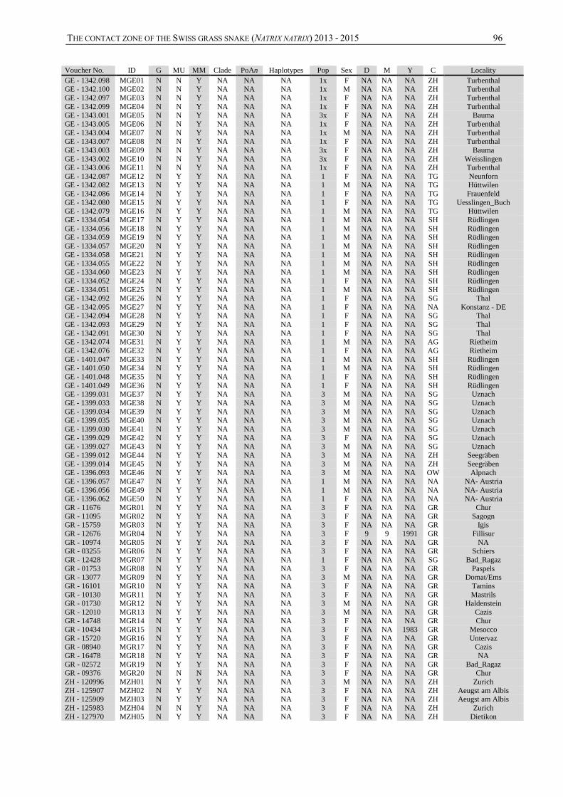
THE CONTACT ZONE OF THE SWISS GRASS SNAKE (NATRIX NATRIX) 2013 - 2015 96
Voucher No. ID G MU MM Clade PoAn Haplotypes Pop Sex D M Y C Locality
GE - 1342.098 MGE01 N N Y NA NA NA 1x F NA NA NA ZH Turbenthal GE - 1342.100 MGE02 N N Y NA NA NA 1x M NA NA NA ZH Turbenthal
GE - 1342.097 MGE03 N N Y NA NA NA 1x F NA NA NA ZH Turbenthal
GE - 1342.099 MGE04 N N Y NA NA NA 1x F NA NA NA ZH Turbenthal GE - 1343.001 MGE05 N N Y NA NA NA 3x F NA NA NA ZH Bauma
GE - 1343.005 MGE06 N N Y NA NA NA 1x F NA NA NA ZH Turbenthal
GE - 1343.004 MGE07 N N Y NA NA NA 1x M NA NA NA ZH Turbenthal GE - 1343.007 MGE08 N N Y NA NA NA 1x F NA NA NA ZH Turbenthal
GE - 1343.003 MGE09 N N Y NA NA NA 3x F NA NA NA ZH Bauma
GE - 1343.002 MGE10 N N Y NA NA NA 3x F NA NA NA ZH Weisslingen GE - 1343.006 MGE11 N N Y NA NA NA 1x F NA NA NA ZH Turbenthal
GE - 1342.087 MGE12 N Y Y NA NA NA 1 F NA NA NA TG Neunforn GE - 1342.082 MGE13 N Y Y NA NA NA 1 M NA NA NA TG Hüttwilen
GE - 1342.086 MGE14 N Y Y NA NA NA 1 F NA NA NA TG Frauenfeld
GE - 1342.080 MGE15 N Y Y NA NA NA 1 F NA NA NA TG Uesslingen_Buch GE - 1342.079 MGE16 N Y Y NA NA NA 1 M NA NA NA TG Hüttwilen
GE - 1334.054 MGE17 N Y Y NA NA NA 1 M NA NA NA SH Rüdlingen
GE - 1334.056 MGE18 N Y Y NA NA NA 1 M NA NA NA SH Rüdlingen GE - 1334.059 MGE19 N Y Y NA NA NA 1 M NA NA NA SH Rüdlingen
GE - 1334.057 MGE20 N Y Y NA NA NA 1 M NA NA NA SH Rüdlingen
GE - 1334.058 MGE21 N Y Y NA NA NA 1 M NA NA NA SH Rüdlingen GE - 1334.055 MGE22 N Y Y NA NA NA 1 M NA NA NA SH Rüdlingen
GE - 1334.060 MGE23 N Y Y NA NA NA 1 M NA NA NA SH Rüdlingen
GE - 1334.052 MGE24 N Y Y NA NA NA 1 F NA NA NA SH Rüdlingen GE - 1334.051 MGE25 N Y Y NA NA NA 1 M NA NA NA SH Rüdlingen
GE - 1342.092 MGE26 N Y Y NA NA NA 1 F NA NA NA SG Thal
GE - 1342.095 MGE27 N Y Y NA NA NA 1 F NA NA NA NA Konstanz - DE GE - 1342.094 MGE28 N Y Y NA NA NA 1 F NA NA NA SG Thal
GE - 1342.093 MGE29 N Y Y NA NA NA 1 F NA NA NA SG Thal
GE - 1342.091 MGE30 N Y Y NA NA NA 1 F NA NA NA SG Thal GE - 1342.074 MGE31 N Y Y NA NA NA 1 M NA NA NA AG Rietheim
GE - 1342.076 MGE32 N Y Y NA NA NA 1 F NA NA NA AG Rietheim
GE - 1401.047 MGE33 N Y Y NA NA NA 1 M NA NA NA SH Rüdlingen GE - 1401.050 MGE34 N Y Y NA NA NA 1 M NA NA NA SH Rüdlingen
GE - 1401.048 MGE35 N Y Y NA NA NA 1 F NA NA NA SH Rüdlingen
GE - 1401.049 MGE36 N Y Y NA NA NA 1 F NA NA NA SH Rüdlingen GE - 1399.031 MGE37 N Y Y NA NA NA 3 M NA NA NA SG Uznach
GE - 1399.033 MGE38 N Y Y NA NA NA 3 M NA NA NA SG Uznach
GE - 1399.034 MGE39 N Y Y NA NA NA 3 M NA NA NA SG Uznach GE - 1399.035 MGE40 N Y Y NA NA NA 3 M NA NA NA SG Uznach
GE - 1399.030 MGE41 N Y Y NA NA NA 3 M NA NA NA SG Uznach
GE - 1399.029 MGE42 N Y Y NA NA NA 3 F NA NA NA SG Uznach GE - 1399.027 MGE43 N Y Y NA NA NA 3 M NA NA NA SG Uznach
GE - 1399.012 MGE44 N Y Y NA NA NA 3 M NA NA NA ZH Seegräben
GE - 1399.014 MGE45 N Y Y NA NA NA 3 M NA NA NA ZH Seegräben GE - 1396.093 MGE46 N Y Y NA NA NA 3 M NA NA NA OW Alpnach
GE - 1396.057 MGE47 N Y Y NA NA NA 1 M NA NA NA NA NA- Austria
GE - 1396.056 MGE49 N Y Y NA NA NA 1 M NA NA NA NA NA- Austria GE - 1396.062 MGE50 N Y Y NA NA NA 1 F NA NA NA NA NA- Austria
GR - 11676 MGR01 N Y Y NA NA NA 3 F NA NA NA GR Chur
GR - 11095 MGR02 N Y Y NA NA NA 3 F NA NA NA GR Sagogn GR - 15759 MGR03 N Y Y NA NA NA 3 F NA NA NA GR Igis
GR - 12676 MGR04 N Y Y NA NA NA 3 F 9 9 1991 GR Fillisur
GR - 10974 MGR05 N Y Y NA NA NA 3 F NA NA NA GR NA GR - 03255 MGR06 N Y Y NA NA NA 3 F NA NA NA GR Schiers
GR - 12428 MGR07 N Y Y NA NA NA 1 F NA NA NA SG Bad_Ragaz
GR - 01753 MGR08 N Y Y NA NA NA 3 F NA NA NA GR Paspels GR - 13077 MGR09 N Y Y NA NA NA 3 M NA NA NA GR Domat/Ems
GR - 16101 MGR10 N Y Y NA NA NA 3 F NA NA NA GR Tamins
GR - 10130 MGR11 N Y Y NA NA NA 3 F NA NA NA GR Mastrils GR - 01730 MGR12 N Y Y NA NA NA 3 M NA NA NA GR Haldenstein
GR - 12010 MGR13 N Y Y NA NA NA 3 M NA NA NA GR Cazis
GR - 14748 MGR14 N Y Y NA NA NA 3 F NA NA NA GR Chur GR - 10434 MGR15 N Y Y NA NA NA 3 F NA NA 1983 GR Mesocco
GR - 15720 MGR16 N Y Y NA NA NA 3 F NA NA NA GR Untervaz GR - 08940 MGR17 N Y Y NA NA NA 3 F NA NA NA GR Cazis
GR - 16478 MGR18 N Y Y NA NA NA 3 F NA NA NA GR NA
GR - 02572 MGR19 N Y Y NA NA NA 3 F NA NA NA GR Bad_Ragaz GR - 09376 MGR20 N N N NA NA NA 3 F NA NA NA GR Chur
ZH - 120996 MZH01 N Y Y NA NA NA 3 M NA NA NA ZH Zurich
ZH - 125907 MZH02 N Y Y NA NA NA 3 F NA NA NA ZH Aeugst am Albis ZH - 125909 MZH03 N Y Y NA NA NA 3 F NA NA NA ZH Aeugst am Albis
ZH - 125983 MZH04 N N Y NA NA NA 3 F NA NA NA ZH Zurich
ZH - 127970 MZH05 N Y Y NA NA NA 3 F NA NA NA ZH Dietikon
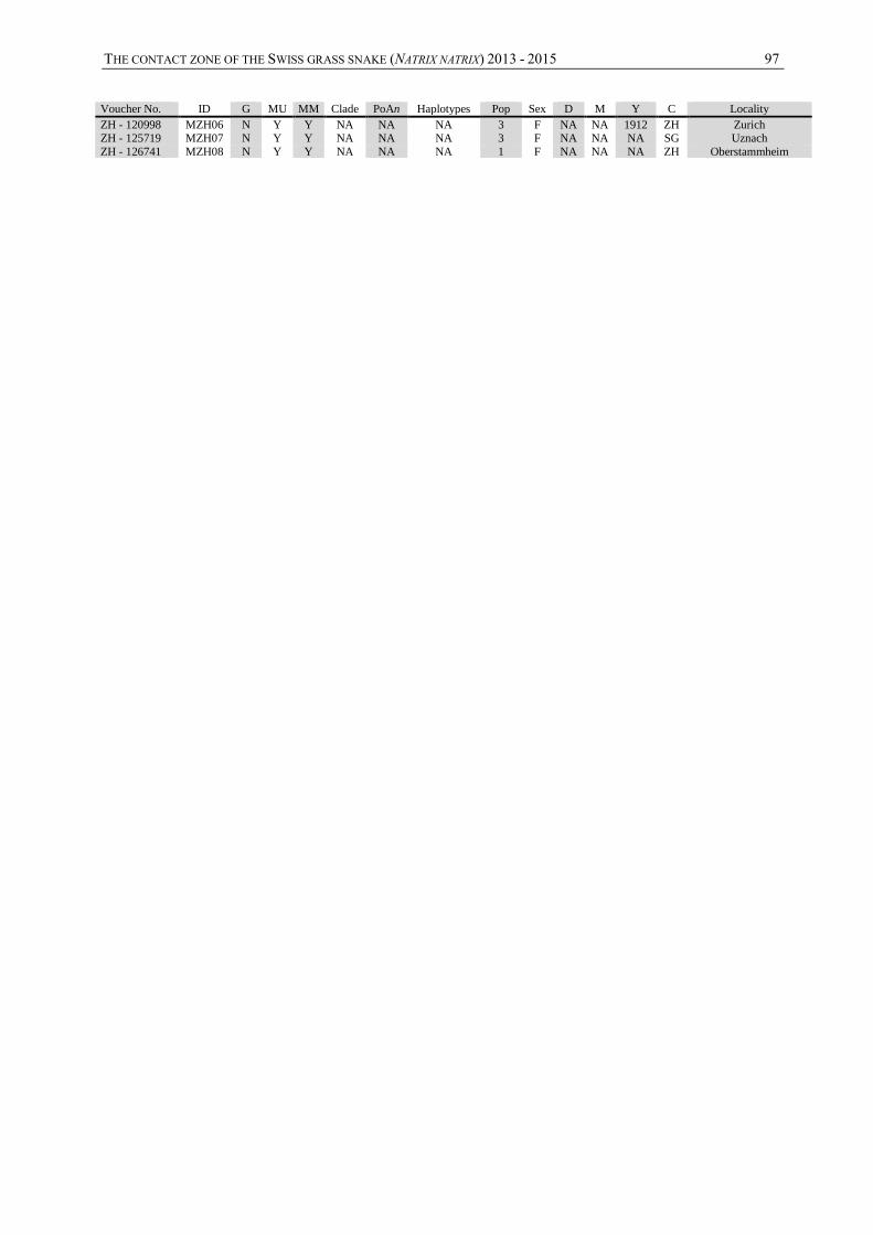
THE CONTACT ZONE OF THE SWISS GRASS SNAKE (NATRIX NATRIX) 2013 - 2015 97
Voucher No. ID G MU MM Clade PoAn Haplotypes Pop Sex D M Y C Locality
ZH - 120998 MZH06 N Y Y NA NA NA 3 F NA NA 1912 ZH Zurich ZH - 125719 MZH07 N Y Y NA NA NA 3 F NA NA NA SG Uznach
ZH - 126741 MZH08 N Y Y NA NA NA 1 F NA NA NA ZH Oberstammheim