The Conjugate Gradient Method - Universitetet i oslo · I So the conjugate gradient method nds the...
28
The Conjugate Gradient Method Tom Lyche Centre of Mathematics for Applications, Department of Informatics, University of Oslo October 21, 2010
Transcript of The Conjugate Gradient Method - Universitetet i oslo · I So the conjugate gradient method nds the...
The Conjugate Gradient Method
Tom Lyche
Centre of Mathematics for Applications,Department of Informatics,
University of Oslo
October 21, 2010
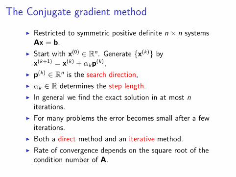
The Conjugate gradient method
I Restricted to symmetric positive definite n × n systemsAx = b.
I Start with x(0) ∈ Rn. Generate {x(k)} byx(k+1) = x(k) + αkp(k),
I p(k) ∈ Rn is the search direction,
I αk ∈ R determines the step length.
I In general we find the exact solution in at most niterations.
I For many problems the error becomes small after a fewiterations.
I Both a direct method and an iterative method.
I Rate of convergence depends on the square root of thecondition number of A.
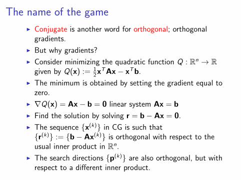
The name of the game
I Conjugate is another word for orthogonal; orthogonalgradients.
I But why gradients?
I Consider minimizing the quadratic function Q : Rn → Rgiven by Q(x) := 1
2xTAx− xTb.
I The minimum is obtained by setting the gradient equal tozero.
I ∇Q(x) = Ax− b = 0 linear system Ax = b
I Find the solution by solving r = b− Ax = 0.
I The sequence {x(k)} in CG is such that{r(k)} := {b− Ax(k)} is orthogonal with respect to theusual inner product in Rn.
I The search directions {p(k)} are also orthogonal, but withrespect to a different inner product.
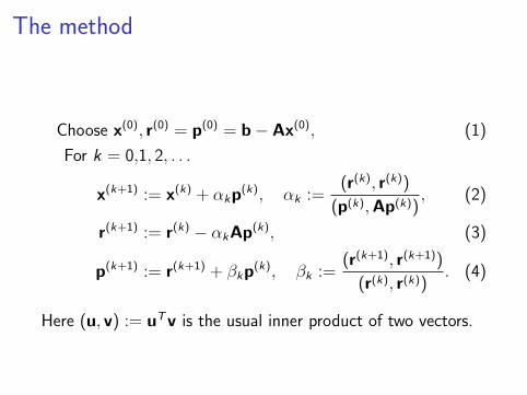
The method
Choose x(0), r(0) = p(0) = b− Ax(0), (1)
For k = 0,1, 2, . . .
x(k+1) := x(k) + αkp(k), αk :=
(r(k), r(k))
(p(k),Ap(k)), (2)
r(k+1) := r(k) − αkAp(k), (3)
p(k+1) := r(k+1) + βkp(k), βk :=
(r(k+1), r(k+1))
(r(k), r(k)). (4)
Here (u, v) := uTv is the usual inner product of two vectors.
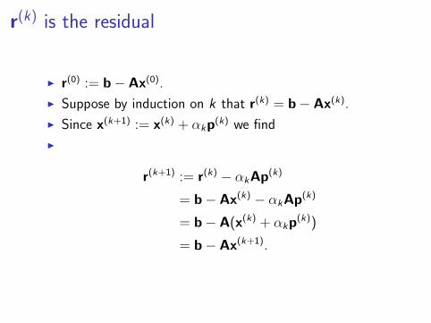
r(k) is the residual
I r(0) := b− Ax(0).
I Suppose by induction on k that r(k) = b− Ax(k).
I Since x(k+1) := x(k) + αkp(k) we find
I
r(k+1) := r(k) − αkAp(k)
= b− Ax(k) − αkAp(k)
= b− A(x(k) + αkp(k))
= b− Ax(k+1).
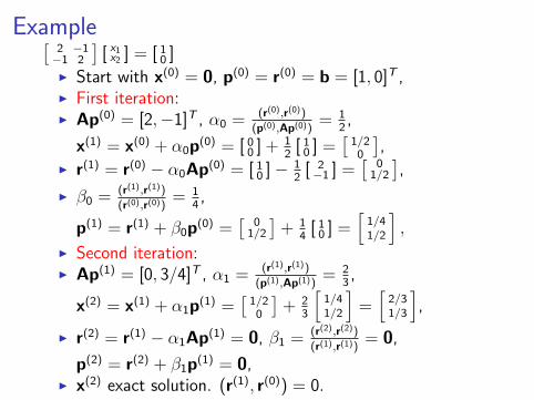
Example[2 −1−1 2
][ x1x2 ] = [ 10 ]
I Start with x(0) = 0, p(0) = r(0) = b = [1, 0]T ,I First iteration:I Ap(0) = [2,−1]T , α0 = (r(0),r(0))
(p(0),Ap(0))= 1
2,
x(1) = x(0) + α0p(0) = [ 00 ] + 12
[ 10 ] =[1/20
],
I r(1) = r(0) − α0Ap(0) = [ 10 ]− 12
[ 2−1 ] =
[0
1/2
],
I β0 = (r(1),r(1))(r(0),r(0))
= 14,
p(1) = r(1) + β0p(0) =[
01/2
]+ 1
4[ 10 ] =
[1/41/2
],
I Second iteration:I Ap(1) = [0, 3/4]T , α1 = (r(1),r(1))
(p(1),Ap(1))= 2
3,
x(2) = x(1) + α1p(1) =[1/20
]+ 2
3
[1/41/2
]=[2/31/3
],
I r(2) = r(1) − α1Ap(1) = 0, β1 = (r(2),r(2))
(r(1),r(1))= 0,
p(2) = r(2) + β1p(1) = 0,I x(2) exact solution. (r(1), r(0)) = 0.
Exact method and iterative method
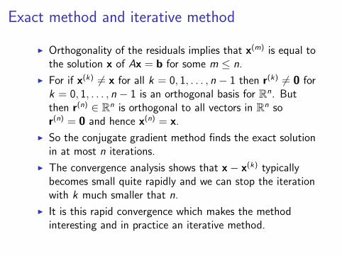
I Orthogonality of the residuals implies that x(m) is equal tothe solution x of Ax = b for some m ≤ n.
I For if x(k) 6= x for all k = 0, 1, . . . , n − 1 then r(k) 6= 0 fork = 0, 1, . . . , n − 1 is an orthogonal basis for Rn. Butthen r(n) ∈ Rn is orthogonal to all vectors in Rn sor(n) = 0 and hence x(n) = x.
I So the conjugate gradient method finds the exact solutionin at most n iterations.
I The convergence analysis shows that x− x(k) typicallybecomes small quite rapidly and we can stop the iterationwith k much smaller that n.
I It is this rapid convergence which makes the methodinteresting and in practice an iterative method.
Conjugate Gradient Algorithm
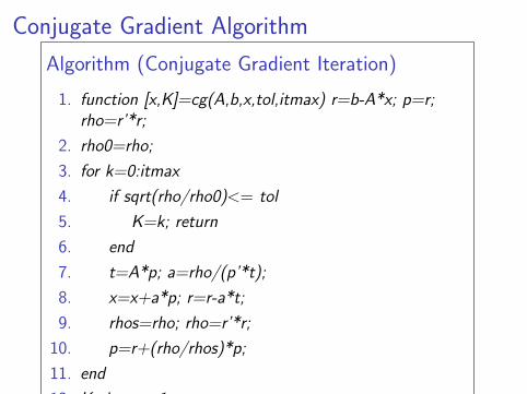
Algorithm (Conjugate Gradient Iteration)
1. function [x,K]=cg(A,b,x,tol,itmax) r=b-A*x; p=r;rho=r’*r;
2. rho0=rho;
3. for k=0:itmax
4. if sqrt(rho/rho0)<= tol
5. K=k; return
6. end
7. t=A*p; a=rho/(p’*t);
8. x=x+a*p; r=r-a*t;
9. rhos=rho; rho=r’*r;
10. p=r+(rho/rhos)*p;
11. end
12. K=itmax+1;
Complexity
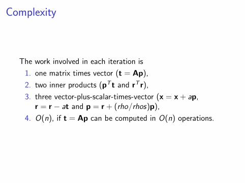
The work involved in each iteration is
1. one matrix times vector (t = Ap),
2. two inner products (pT t and rT r),
3. three vector-plus-scalar-times-vector (x = x + ap,r = r − at and p = r + (rho/rhos)p),
4. O(n), if t = Ap can be computed in O(n) operations.
A family of test problems
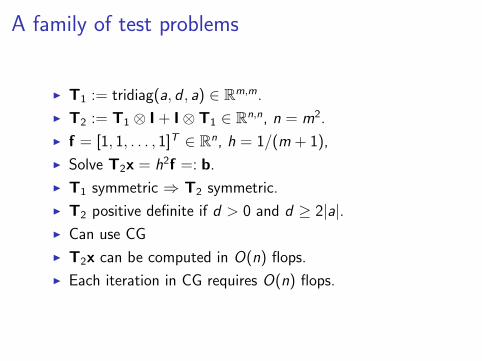
I T1 := tridiag(a, d , a) ∈ Rm,m.
I T2 := T1 ⊗ I + I⊗ T1 ∈ Rn,n, n = m2.
I f = [1, 1, . . . , 1]T ∈ Rn, h = 1/(m + 1),
I Solve T2x = h2f =: b.
I T1 symmetric ⇒ T2 symmetric.
I T2 positive definite if d > 0 and d ≥ 2|a|.I Can use CG
I T2x can be computed in O(n) flops.
I Each iteration in CG requires O(n) flops.
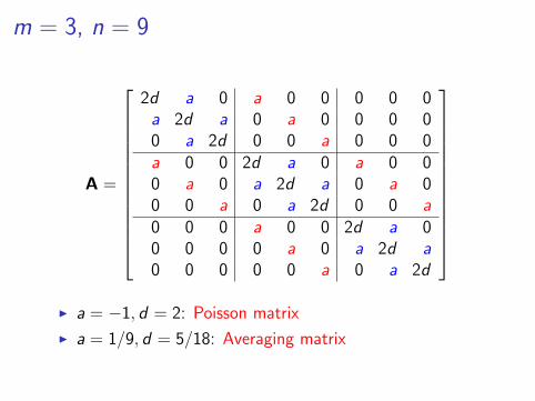
m = 3, n = 9
A =
2d a 0 a 0 0 0 0 0a 2d a 0 a 0 0 0 00 a 2d 0 0 a 0 0 0a 0 0 2d a 0 a 0 00 a 0 a 2d a 0 a 00 0 a 0 a 2d 0 0 a0 0 0 a 0 0 2d a 00 0 0 0 a 0 a 2d a0 0 0 0 0 a 0 a 2d
I a = −1, d = 2: Poisson matrix
I a = 1/9, d = 5/18: Averaging matrix
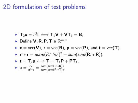
2D formulation of test problems
I T2x = h2f ⇐⇒ T1V + VT1 = B,
I Define V,R,P,T ∈ Rm,m
I x = vec(V), r = vec(R), p = vec(P), and t = vec(T).
I r′ ∗ r = norm(R ,′ fro ′)2 = sum(sum(R. ∗ R)).
I t = T2p⇐⇒ T = T1P + PT1.
I a = r′∗rp′∗t = sum(sum(R.∗R))
sum(sum(P.∗T)) .
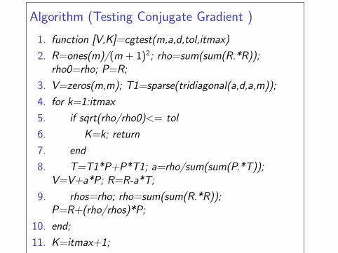
Algorithm (Testing Conjugate Gradient )
1. function [V,K]=cgtest(m,a,d,tol,itmax)
2. R=ones(m)/(m + 1)2; rho=sum(sum(R.*R));rho0=rho; P=R;
3. V=zeros(m,m); T1=sparse(tridiagonal(a,d,a,m));
4. for k=1:itmax
5. if sqrt(rho/rho0)<= tol
6. K=k; return
7. end
8. T=T1*P+P*T1; a=rho/sum(sum(P.*T));V=V+a*P; R=R-a*T;
9. rhos=rho; rho=sum(sum(R.*R));P=R+(rho/rhos)*P;
10. end;
11. K=itmax+1;
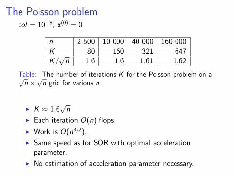
The Poisson problemtol = 10−8, x(0) = 0
n 2 500 10 000 40 000 160 000K 80 160 321 647K/√
n 1.6 1.6 1.61 1.62
Table: The number of iterations K for the Poisson problem on a√n ×√n grid for various n
I K ≈ 1.6√
n
I Each iteration O(n) flops.
I Work is O(n3/2).
I Same speed as for SOR with optimal accelerationparameter.
I No estimation of acceleration parameter necessary.
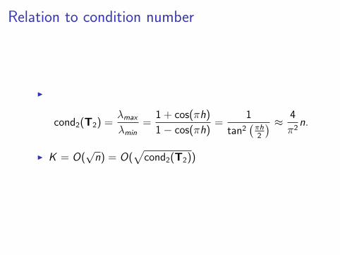
Relation to condition number
I
cond2(T2) =λmax
λmin=
1 + cos(πh)
1− cos(πh)=
1
tan2(πh2
) ≈ 4
π2n.
I K = O(√
n) = O(√
cond2(T2))
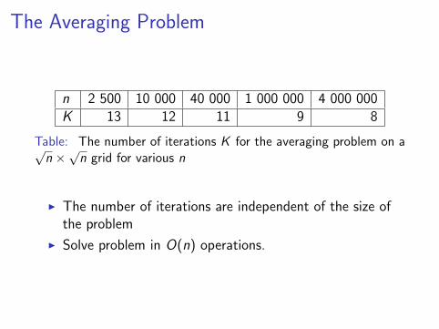
The Averaging Problem
n 2 500 10 000 40 000 1 000 000 4 000 000K 13 12 11 9 8
Table: The number of iterations K for the averaging problem on a√n ×√n grid for various n
I The number of iterations are independent of the size ofthe problem
I Solve problem in O(n) operations.
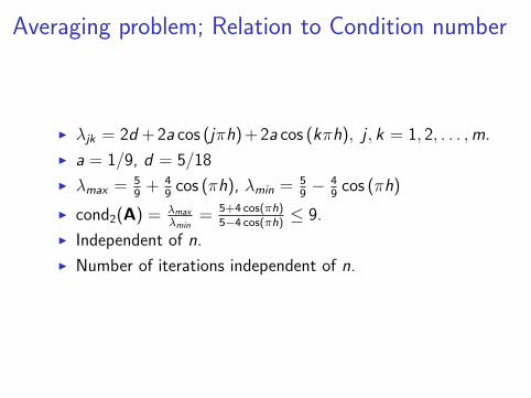
Averaging problem; Relation to Condition number
I λjk = 2d + 2a cos (jπh) + 2a cos (kπh), j , k = 1, 2, . . . ,m.
I a = 1/9, d = 5/18
I λmax = 59
+ 49
cos (πh), λmin = 59− 4
9cos (πh)
I cond2(A) = λmax
λmin= 5+4 cos(πh)
5−4 cos(πh) ≤ 9.
I Independent of n.
I Number of iterations independent of n.
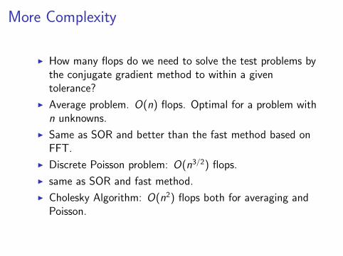
More Complexity
I How many flops do we need to solve the test problems bythe conjugate gradient method to within a giventolerance?
I Average problem. O(n) flops. Optimal for a problem withn unknowns.
I Same as SOR and better than the fast method based onFFT.
I Discrete Poisson problem: O(n3/2) flops.
I same as SOR and fast method.
I Cholesky Algorithm: O(n2) flops both for averaging andPoisson.
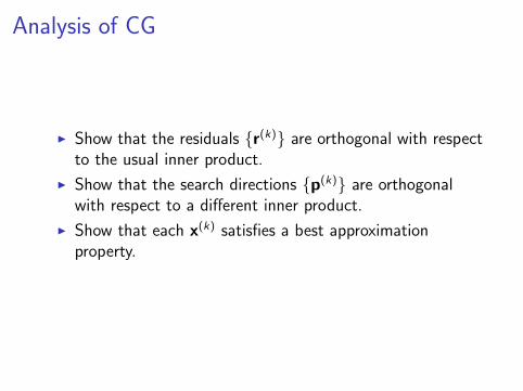
Analysis of CG
I Show that the residuals {r(k)} are orthogonal with respectto the usual inner product.
I Show that the search directions {p(k)} are orthogonalwith respect to a different inner product.
I Show that each x(k) satisfies a best approximationproperty.
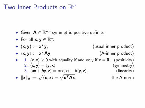
Two Inner Products on Rn
I Given A ∈ Rn,n symmetric positive definite.
I For all x, y ∈ Rn:
I (x, y) := xTy, (usual inner product)
I 〈x, y〉 := xTAy (A-inner product)
I 1. 〈x, x〉 ≥ 0 with equality if and only if x = 0. (positivity)2. 〈x, y〉 = 〈y, x〉 (symmetry)3. 〈ax+ by, z〉 = a〈x, z〉+ b〈y, z〉. (linearity)
I ‖x‖A :=√〈x, x〉 =
√xTAx. the A-norm
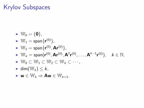
Krylov Subspaces
I W0 = {0},I W1 = span{r(0)},I W2 = span{r(0),Ar(0)},I Wk = span(r(0),Ar(0),A2r(0), . . . ,Ak−1r(0)), k ∈ N,I W0 ⊂W1 ⊂W2 ⊂Wk ⊂ · · · ,I dim(Wk) ≤ k ,
I w ∈Wk ⇒ Aw ∈Wk+1.
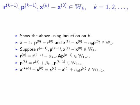
r(k−1),p(k−1), x(k) − x(0) ∈Wk , k = 1, 2, . . . ,
I Show the above using induction on k .
I k = 1: p(0) = r(0) and x(1) − x(0) = α0p(0) ∈W1.
I Suppose r(k−1),p(k−1), x(k) − x(0) ∈Wk .
I r(k) = r(k−1) − αk−1Ap(k−1) ∈Wk+1.
I p(k) = r(k) + βk−1p(k−1) ∈Wk+1.
I x(k+1) − x(0) = x(k) − x(0) + αkp(k) ∈Wk+1.
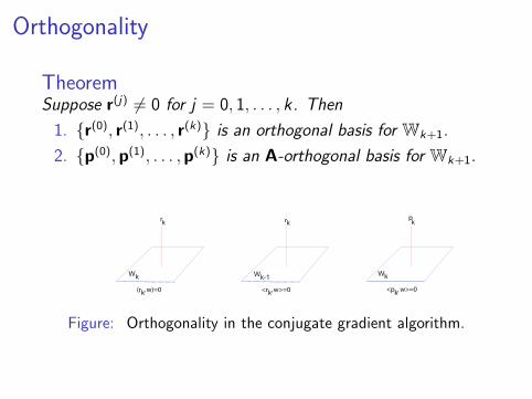
Orthogonality
TheoremSuppose r(j) 6= 0 for j = 0, 1, . . . , k. Then
1. {r(0), r(1), . . . , r(k)} is an orthogonal basis for Wk+1.
2. {p(0),p(1), . . . ,p(k)} is an A-orthogonal basis for Wk+1.
rk
Wk
(r , w)=0k
k
Wk-1
<r , w>=0k
r k
Wk
<p , w>=0
p
k
Figure: Orthogonality in the conjugate gradient algorithm.
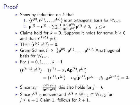
ProofI Show by induction on k that
1. {r(0), r(1), . . . , r(k)} is an orthogonal basis for Wk+1.
2. p(j) = r(j) −∑j−1
i=0〈r(j),p(i)〉〈p(i),p(i)〉p
(i) 6= 0, j ≤ k.
I Claims hold for k = 0. Suppose it holds for some k ≥ 0and that r(k+1) 6= 0.
I Then (r(k), r(i)) = 0.I Gram-Schmidt ⇒ {p(0),p(1), . . . ,p(k)} A-orthogonal
basis for Wk+1.I For j = 0, 1, . . . , k − 1
(r(k+1), r(j)) = (r(k) − αkAp(k), r(j))
= (r(k), r(j))− αk〈p(k),p(j) − βj−1p(j−1)〉 = 0.
I Since αk = (r(k),r(j))
〈p(k),p(j)〉 this also holds for j = k .
I Since r(j) is nonzero and r(j) ∈Wj+1 ⊂Wk+2 forj ≤ k + 1 Claim 1. follows for k + 1.
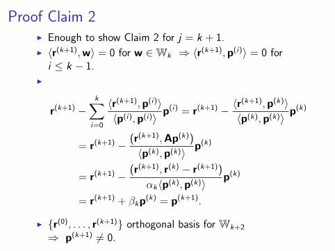
Proof Claim 2I Enough to show Claim 2 for j = k + 1.
I 〈r(k+1),w〉 = 0 for w ∈Wk ⇒ 〈r(k+1),p(i)〉 = 0 fori ≤ k − 1.
I
r(k+1) −k∑
i=0
〈r(k+1),p(i)〉〈p(i),p(i)〉
p(i) = r(k+1) − 〈r(k+1),p(k)〉〈p(k),p(k)〉
p(k)
= r(k+1) − (r(k+1),Ap(k))
〈p(k),p(k)〉p(k)
= r(k+1) − (r(k+1), r(k) − r(k+1))
αk〈p(k),p(k)〉p(k)
= r(k+1) + βkp(k) = p(k+1).
I {r(0), . . . , r(k+1)} orthogonal basis for Wk+2
⇒ p(k+1) 6= 0.
Best Approximation Property of x(k)
CorollarySuppose Ax = b, where A ∈ Rn,n is symmetric positivedefinite and {x(k)} is generate by the conjugate gradientalgorithm. Then x(k) − x(0) is the best approximation tox− x(0) in the A-norm
‖x− x(k)‖A = minw∈Wk
‖x− x(0) −w‖A. (5)
In particular, if x(0) = 0 then x(k) is the best approximation tox in the A-norm.
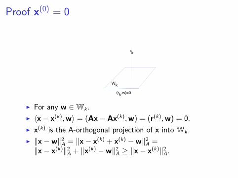
Proof x(0) = 0
rk
Wk
(r , w)=0k
I For any w ∈Wk .
I 〈x− x(k),w〉 = (Ax− Ax(k),w) = (r(k),w) = 0.
I x(k) is the A-orthogonal projection of x into Wk .
I ‖x−w‖2A = ‖x− x(k) + x(k) −w‖2A =‖x− x(k)‖2A + ‖x(k) −w‖2A ≥ ‖x− x(k)‖2A.
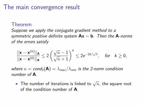
The main convergence result
TheoremSuppose we apply the conjugate gradient method to asymmetric positive definite system Ax = b. Then the A-normsof the errors satisfy
||x− x(k)||A||x− x(0)||A
≤ 2
(√κ− 1√κ + 1
)k
≤ 2e−2k/√κ, for k ≥ 0,
where κ = cond2(A) = λmax/λmin is the 2-norm conditionnumber of A.
I The number of iterations is linked to√κ, the square root
of the condition number of A.


![The Conjugate Gradient Method...Conjugate Gradient Algorithm [Conjugate Gradient Iteration] The positive definite linear system Ax = b is solved by the conjugate gradient method.](https://static.fdocuments.net/doc/165x107/5e95c1e7f0d0d02fb330942a/the-conjugate-gradient-method-conjugate-gradient-algorithm-conjugate-gradient.jpg)