) j

//'i:, 7 <_ N95- 32430

The Composite Classification Problem

in Optical Information Processing

Final Report

NASA/ASEE Summer Faculty FeLlowship Program--1994

Johnson Space Center

Prepared By:

Academic Rank:

Conege and Department:

NASA/JSC

Directorate:

Division:

Branch:

JSC Colleague:

Date Submitted:

Contract Number:

Eric B. Hall, Ph.D.

Assistant Professor

Southern Methodist University

Dept. of Electrical EngineeringDallas, Texas 75275

Engineering

Tracking and Communications

Tracking Techniques

Richard D. Juday

August 5, 1994

NGT-44-005-803

13-1

https://ntrs.nasa.gov/search.jsp?R=19950026009 2018-05-20T00:31:01+00:00Z

ABSTRACT

Optical pattern recognition allows objects to be recognized from their images and

permits their positional parameters to be estimated accurately in real time. The

guiding principle behind optical pattern recognition is that a lens focusing a beam

of coherent light modulated with an image produces the two-dimensional Fourier

transform of that image. When the resulting output is further transformed by the

matched filter corresponding to the original image, one obtains the autocorrelation

function of the priginal image, which has a peak at the origin. Such a device is called

an optical correlator and may be used to recognize and locate the image for which it is

designed. (From a practical perspective, an approximation to the matched filter must

be used since the spatial light modulator (SLM) on which the filter is implemented

usually does not allow one to independently control both the magnitude and phase of

the filter.) Generally, one is not just concerned with recognizing a single image, but is

instead interested in recognizing a variety of rotated and scaled views of a particular

image. In order to recognize these different views using an optical correlator, one

may select a subset of these views (whose elements are called training images) and

then use a composite filter that is designed to produce a correlation peak for each

training image. Presumably, these peaks should be sharp and easily distinguishable

from the surrounding correlation plane values. In this report we consider two areas

of research regarding composite optical correlators. First, we consider the question

of how best to choose the training images that are used to design the composite

filter. With regard to quantity, the number of training images should be large enough

to adequately represent all possible views of the targeted object yet small enough to

ensure that the resolution of the filter is not exhausted. As for the images themselves,

they should be distinct enough to avoid numerical difficulties yet similar enough to

avoid gaps in which certain views of the target will be unrecognized. One method

that we introduce to study this problem is called probing and involves the creation of

artificial imagery. The second problem we consider involves the classification of the

composite filter's correlation plane data. In particular, we would like to determine

not only whether or not we are viewing a training image, but, in the former case, we

would like to determine which training image is being viewed. This second problem

is investigated using traditional M-ary hypothesis testing techniques.

13-2

INTRODUCTION _= BACKGROUND

A Review of Quadratic Classifiers Consider a random vector X taking values

in R d with a multivariate 1 Gaussian density function

1 1

f(x) - (27r)d/2 I_l exp (---_(x -- #)-r_-l(x -- tz))(:)

(7 dwhere g = E[X] = [g,],d= 1 and E = E[(X -/_)(X - #)-r] = [ ,ill,j=1" Note that this

distribution is completely characterized by d + ½d(d + 1) parameters. We sometimes

denote this distribution by N(#, E) where the covariance matrix E is a symmetric,

nonnegative definite matrix. In writing expression (1), we have assumed that E is in

fact positive definite, and hence invertible. If, instead, E is singular then aTx = 0 a.s.

for some nonzero vector a from R d. In such a case, we say that the distribution of X is

degenerate. If E[larXI 2] > 0 for each nonzero a C R d then the covariance matrix E is

positive definite. The nonnegative square root of the value (x - tz)VE-l(x - #) in the

exponent of (1) is called the Mahalanobis distance from x to the mean #. Note that

a set of points with equal Mahalanobis distance to the mean forms a hyperellipsoidin IRd. 2

Our interest lies with the a posterior density function

p(x[t_)P(t_)

p(t, lx) = p(x)

where t_ denotes an image with an a priori probability of P(ti). After taking the

natural log of the a posterior density function and neglecting the terms that do not

change with i, 3 we obtain a discriminant function of the form gi(x) = lnp(x]t_) +

in P(ti). Assume now that p(xlt{ ) is a multivariate Gaussian density function with

mean vector #_ and covariance matrix E_. In this case, it follows that

1 d ln(27r)- 2 InI_,l ÷ InP(ti)g,(x) = -:(x - ,_):Z;:(_ - ,,) - : (2)

If E = cr2I, then equation (2) reduces to

gi(_) = -IIx - _i,2,,+ lnP(ti) (3)2o-2

:The components of X are said to be jointly or mutually Gaussian. Whereas a sum of Gaussianrandom variables need not be Gaussian, and uncorrelated Gaussian random variables need not beindependent, these useful properties do hold when the random variables are jointly Gaussian.

2For more information concerning the topics in this section, see [3] or [4].3Throughout this discussion the gi's are equal up to additive, constant functions of i and/or

multiplicative, positive, constant functions of i.

13-3

where ]Ix - #ill 2 - (x - #i)T(X --#i). Note that if the a priori probabilities are equal

then this test assigns x to the category that has the nearest mean, where distance

is determined using the previous norm. This type of classifier is called a minimum

distance classifier. However, if we expand gi a step further (retaining all but the xTx

term), equation (3) reduces to

g (x) = -Tx + (4)

where a_ = #i/_2 and _ = -#_r#_/2a2 + ln P(t_). A test of this form is called

a correlator detector or linear detector. As indicated by equation (4), the decision

boundaries induced by equation (3) are hyperplanes.

Next, consider the case in which P,_ is equal to some constant matrix 2 for all i.

In this case, equation (2) reduces to

1

9i( ) = - u,)Tz-l(z - + in P(td.

If the a priori probabilities are equal then this test assigns x to the distribution whose

mean has the smallest Mahalanobis distance to x. Expanding further, however, we

again obtain a test function of the form

= +

where this time ai = E-l#i and 3i 1 r,-,-1= -7#i 2, I_i+lnP(ti). Note that again we have

obtained a linear classifier and that our decision boundaries are hyperplanes.

In the general case, equation (2) may be written as

gi(x) = xT Aix + c_Tx + _i

, -1 1. T_-I _ln[Z,] + lnP(t,) Notewhere Ai =-TEi , oti = E_I/_i, and fli #i -= -_/z i z_ithat this test function is quadratic and that the corresponding decision boundaries

are hyperquadrics.

The Classification Problem &= Bayesian Inference Consider No classes of ob-

jects denoted by wo,..., Wgo. Assume that object class Wk contains Nk training images

denoted by Tlk, T2k,..., TNkk. Let NT = _1 Nk denote the total number of training

images. The standard classification problem seeks a partition of the "signal space"

into NT classification regions denoted by R1,...,RNr. The composite classification

problem, on the other hand, seeks a partition of the "signal space" into No regions

denoted by C1,..., Cyo; that is, each region corresponds to a different object class

where each object class can contain many different training images.

Let NF denote the number of composite filters that are formed from the training

images, and let NM denote the number of "features" that are required by the chosen

13-4

correlationmetric. Then, the dimensionn of our signal space is given by NFNM. (In

this context, a "signal" corresponds to the output of our composite filter. Our goal

is to classify these outputs into their corresponding object classes. The goal of the

standard classification problem would be to map each possible output to the training

image that produced it. Note that, for the moment, we are assuming that only

training images are available as inputs to our system.) Our goals, once we develop

our test, will be to choose the training image groups and composite filters so that (1)

the distributions of the test statistics can be estimated accurately with as few samples

as possible, and, (2) the distributions of the test statistics do not significantly overlap.

(The first goal has pragmatic motivations, and the second goal reflects the standard

desire that our test be as close to singular as possible.)

Let X denote our signal; that is, let X be a random vector taking values in _ NMNF

that represents the NM outputs of each of the NF filters. Let PT_k (x) be a probability

density function for X when the training image Tik is used as the input. Let IIik

denote the a priori probability that the input to our system is training image Tik. We

will use these a priori probabilities to develop a Bayesian test. One assumption at

this point is, of course, that these probabilities both exist and are known. Further, we

will assume that the sum of the rIik's over all possible training images is unity. That

is, as mentioned above, we will continue to assume that only training images are input

into our system. Based upon these assumptions we have the following expression for

a probability density function for the output of our system:

No N,

pT(x) = Z Z •k=l i=1

Note that this density is only exact if our inputs are exclusively training images. In a

more general setting in which our inputs need not be training images we would hope

that this density would be a close approximation of the true density of the output.

(An interesting problem would be to investigate the behavior of this approximation

as Nr

The Standard Classifier For a standard classifier, we let No = N:r; that is,

our object classes are singleton sets each containing a single training image. In this

case, we will denote Tik by Tk and IIik by IIk. According to the usual Bayes formula,

we have

p(TklX = x) -- PT_(:IlIkpr(:)

where p(TklX = x) denotes the conditional probability that Tk was input given that

we observed x. Our Bayesian hypothesis test then is to assign x to Tk if and only if

p(Tk[X = z) >_ p(Ti[X = x) for all/ = 1,..., NT. (That is, we choose the training

image corresponding to a maximum a posterior distribution.)

13-5

The Composite Classifier For a compositeclassifier,No is less than (usually

much less than) NT. Let P_k (x) be a probability density function for X when the

input is a training image from the object class wi. Let Ak be the a priori probability

that the input will be from class wi. (Yet again, we are assuming that the input will

always be a training image.) Note that

Nk

hk = _ IIjk.j=l

Also, note that

1 Nk

j=l

and further, using Bayes' formula, note that

Nk

p(wk[X = x)- p_(x)Ak _ 1 _pr, k(x)iiik (5)

where p(wk IX = x) is the conditionalthat x is observed. Our test in this

p(wk[X = x) >_ p(wj[X = x) for all j

and only if

for all j = 1,...,No.

probability that the input is from class _k given

case assigns x to object class wk if and only if

= 1,..., No. That is, we assign x to class wk if

(x)II

We will now assume that pTjk(x) is an n-variate Gaussian density function with

mean vector mjk and covariance matrix Cjk where we recall that n = NMNF. Note

that, in this case, pT(x) and p_k(x) are mixtures of multivariate Gaussian densities,

which, of course, can be far from Gaussian. Several problems present themselves at

this point. First, the rather rueful distribution of X does not bode well for analytic

solutions. 4 Second, the parameters mjk and Cjk are rarely known and hence often

must be estimated. These estimates may then substituted into the test given above.

Unfortunately, when this substitution is done, our test is generally no longer Bayesian,

and hence, need no longer satisfy any desired optimality property such as minimum

probability of error. 5 Although the test statistic is difficult to work with, one possible

4"1'obe precise, it is only our approximation of the distribution of X that is a mixture of Gaussian

distributions unless we assume that our inputs will only be training images. Of course, there is noreason to expect that the true distribution of X is any less rueful than our approximation of thatdistribution.

S2'he likelihood ratio corresponding to such a test is sometimes said to be a generalized likelihoodratio, particularly when the unknown parameters are replaced with maximum likelihood estimates.

13-6

simplification involvescoordinatetransformationsthat simplify the calculation of theMahalanobisdistancesin the exponents.

TRAININGIMAGESIn the previous section, we assumedthat the input to our system was always atraining image, that the output of our systemgiven that the input was a trainingimage wasGaussian,and that the output of our systemgiven that the input wasatraining imagefrom a particular object classwasequal in distribution to a mixtureof Gaussiandistributions.

Therearetwo typesof non-training images.A .first category non-training image is

an unknown view of a known object. Ideally, this type of image will be close enough to

an appropriate training image so that their distributions will have significant overlap.

A second category non-training image is an image of an object that is not intended

to be recognized. IdeMly, this type of image should be far away from the training

images so that its distribution will not have significant overlap with that of any

training image.

Of course, as we approach the ideal situation, we are generally going to need an

ever increasing supply of training images. While a larger number of training images

would be helpful when the input is a non-training image, it would also increase the

complexity of our system and it would decrease the performance when the input

actually is a training image. What we need is: (1) a method of determining how many

training images we need to meet some desired goal, and (2) a method of obtaining

appropriate additional training images when such images are required. In the next

section, we will consider both of these problems.

Probing In [2] the term probing is introduced and used to describe the creation of

artificial images to improve and analyze pattern recognition algorithms. A determin-

istic pattern recognition algorithm is simply a function mapping the set of all possible

images to some decision set. Ideally, one would choose this function by considering

each possible image in turn and determining for each the appropriate decision that

should be made if that image appears as the input to our system. Unfortunately, how-

ever, such a design procedure is generally not tractable due to the enormous number

of possible input scenes. (For example, there are over 1039'°°° different 128 by 128

pixel input images with 256 gray scales.) It is at this point that probing becomes

useful since it allows one to intelligently sample this enormous image space in order

to select images for which a pattern recognition scheme can be designed.

We have identified three different methods of probing that appear promising with

regard to optical information processing. First, probing can be used to form a "map"

of the image space. As an example, consider two images 11 and 12 from the image

space consisting of all N × N pixel images composed of M gray scale levels. (Note

13-7

that suchan imagecanbeviewedasa point in the set {0,1,..., M- 1} N2.) For each

value of p C [0, 1], let Vp be a random object taking values in {0, 1,..., M - 1} N_ such

that each pixel value in Vp is equal with probability p to the corresponding pixel value

in I2 and is equal with probability 1 -p to the corresponding pixel value in I1. 6 (Note

that V0 = I1 and V1 = I2. Note also that if a particular pixel in I1 and/2 agree then

they also agree with the corresponding pixel in Vp. Thus, the pixel variance in Vp is

only positive for pixels at which It and/2 disagree.) As p increases from 0 to 1, 7 our

decision algorithm (when applied to Vp) will on average no longer recognize It at some

point pt and will begin instead to recognize Is at some point P2. These average values

of p allow us to determine when images are "adjacent" and to recognize the possible

existence of a "hole" between/1 and I2. A map of this sort allows us to distinguish

between two procedures that perform the same when the inputs are always training

images. Further, we could possibly use a realization of Vp where pt < p < p2 to

fill such a hole in our set of training images. Of course, different realizations of Vp

for some fixed choice of p E (0, 1) could be quite different. (A similar procedure is

described in [7] where sections of training images axe randomly selected and weighted

to form what is called a synthetic reference object.)

Second, probing can be used to measure the robustness of a pattern recognition

algorithm. For a training image T and a nonnegative value 0, let Uo be an image

(i.e. a random object taking values in {0, 1,..., M - 1} N2) such that each pixel value

in Ue has a mean equal to the corresponding pixel value in T and has a variance

equal to 8. Note that Uo = T a.s. The average value of 0 at which T is no longer

recognized provides an indication of the robustness of our algorithm with respect to

that particular training image. Presumably this value should be large and should

not vary widely among the different training images. Tests of this sort allow us

to distinguish between two procedures that perform identically when the inputs are

always training images.

Third, probing can be employed in which the pixel values in the synthesized image

axe not statistically independent. By introducing some sort of spatially localized

dependence, we can analyze a situation in which a pixel in the synthesized image is

more likely to be from a particular training image if its neighboring pixel values are

also from that training image.

6In addition, one could further perturb the image by choosing for some given gray scale value

M0, a realization of a random variable with a unimodal distribution on {0, 1,..., M - 1} centered

at M0.

ZNotice that from an information theoretic standpoint, the "uncertainty" is maximized when

p = 1/2

13-8

COMPOSITE CORRELATION

Synthetic Discriminant Functions The synthetic discriminant function approach

uses a linear combination of training images to create a composite image that is cross

correlated with the input to the system. The weights in the linear combination are

chosen so that the cross correlation at the origin is the same for all training images

from the same class. (The resulting filter is sometimes called an Equal Correlation

Peak (ECP) Synthetic Discriminant Function (SDF).) For example, if we have N

training images sl(z, y),..., sy(x, y), then our composite image would be of the form

and the c_,'s would be chosen so that

co

--(DO --oo

for i = 1,..., N where the c_'s are preselected constants. Modifications of the stan-

dard SDF approach exist that impose other constraints. For example, Minimum

Variance SFD (MVSDF) minimizes the output noise variance and the Minimum Av-

erage Correlation Energy (MACE) filter attempts to produce sharp correlation peaks

at the origin of the output.

Let H(u, v) denote the Fourier transform of the composite image h(x, y); that is,

letoO oo

--00 --O0

Note that

--O0 --_

Also, let Si denote the Fourier transform of the ith training image sl for i = 1,..., N.

Further, for an element x from 1_N or C N let ._ denote the corresponding element in

R N×N or C N×N that is obtained by placing x along the diagonal and 0 elsewhere.

That is, let

xi ifi=j5_j= 0 ifi#j.

Finally, assume that the input to our system is corrupted with an additive, zero mean,

wide sense stationary noise process N(x,y) with power spectral density PN(u,v).

That is,

oo oo

PN(U,V) = ./ ./ E[N(x + r,y + _ ) N* (x , y ) ] e-J2"_("_'+:'v) &- dA

--¢_ --CO

13-9

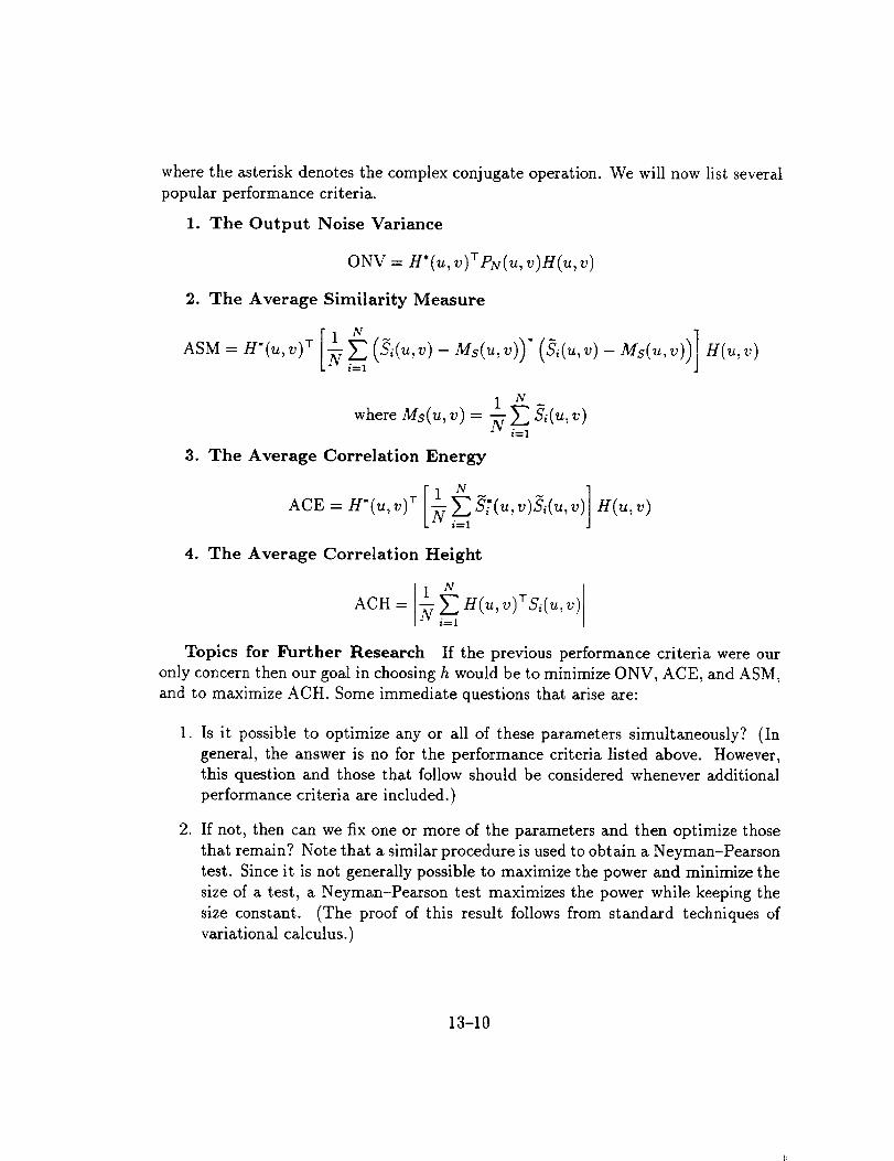
where the asterisk denotes the complex conjugate operation. We will now list several

popular performance criteria.

1. The Output Noise Variance

0NV= H*(u,v)rpy(u,v)H(u,v)

2. The Average Similarity Measure

ASM = H'(u,v)T [N

N

i=1

H(u,v)

1 N

where Ms(u, v) = -_ __, Si(u, v)i=1

3. The Average Correlation Energy

ACE = H'(u,v)T [Ni----1

4. The Average Correlation Height

ACH = j1 _ H(u,v)TSi(u,v)

Topics for Further Research If the previous performance criteria were our

only concern then our goal in choosing h would be to minimize ONV, ACE, and ASM,

and to maximize ACH. Some immediate questions that arise are:

1. Is it possible to optimize any or all of these parameters simultaneously? (In

general, the answer is no for the performance criteria listed above. However,

this question and those that follow should be considered whenever additional

performance criteria are included.)

2. If not, then can we fix one or more of the parameters and then optimize those

that remain? Note that a similar procedure is used to obtain a Neyman-Pearson

test. Since it is not generally possible to maximize the power and minimize the

size of a test, a Neyman-Pearson test maximizes the power while keeping the

size constant. (The proof of this result follows from standard techniques of

variational calculus.)

13-10

. There are numerous paradoxes that arise in the Neyman-Pearson theory. Do

similar difficulties arise here? For example, in a Neyman-Pearson test, strange

results can occur if the false alarm rate is chosen to be large in a test that is

almost singular. Conversely, situations exist in which the power exceeds the

false alarm rate by an arbitrarily small value.

, An optimal trade-off filter is obtained by fixing all but 6ne of the parameters

and optimizing the other. Is this necessary? Might it be possible to fix fewer

parameters and then optimize those that remain?

Minimum Euclidean Distance Optimal Filters Our goal in this section is to

extend the results in [5] to include composite filters. In particular, we will first

seek an algorithm by which the output of the MEDOF algorithm can be classified

by statistical inference into training image classes. The following steps follow the

procedure suggested in [1]:

1. Separate the training images into object classes. The first step is to

select the training images and object classes. Each object class should correspond to

a different object that we wish to recognize. The training images within each object

class should be chosen to adequately describe the different expected orientations of

the object they represent.

2. Create the filters by which these training images will be distin-

guished. One way in which this step could be achieved would be to create a com-

posite image from each object class based upon the training images in that object

class. These composite images could then be used to create composite filters whose

combined outputs would comprise the components of our output random vector X.

(That is, we would let NF = No.)

3. Estimate the mean and covariance matrix for each class. We have

assumed that the output of our system given that the input is a specific training image

Tjk will be multivariate Gaussian with mean mjk and covariance matrix Cjk. We

will estimate these parameters via standard techniques. In particular, if we observe

xx,..., xy when training image Tjk is our input then we will estimate mjk via

1 N

i--1

and we will estimate Cjk via

1 N

i----1

13-11

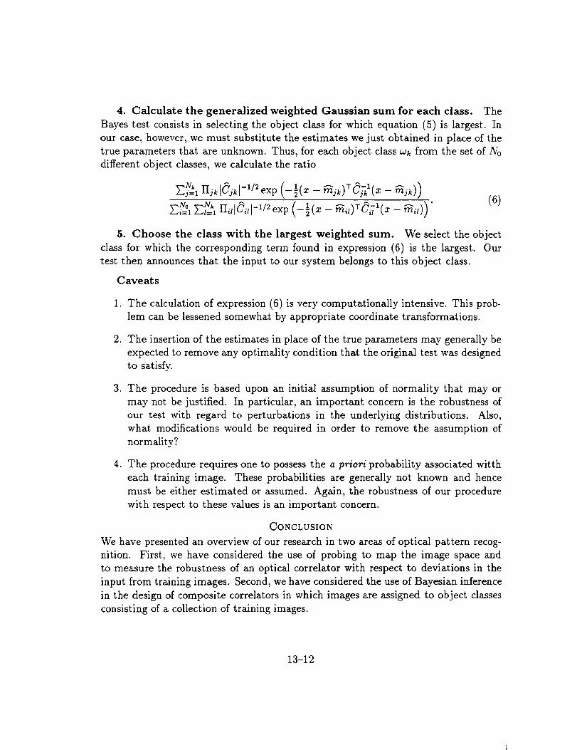
4. Calculate the generalized weighted Gaussian sum for each class. The

Bayes test consists in selecting the object class for which equation (5) is largest. In

our case, however, we must substitute the estimates we just obtained in place of the

true parameters that are unknown. Thus, for each object class Wk from the set of No

different object classes, we calculate the ratio

Nk 1E_=a IljklC kl - /2exp (-i(x _ "r ^-1

E/N01 Nk 1 "]O,=, II,,IC,/I -a/2 exp (-7(z- _,,)rC,T_(x - _.))(6)

5. Choose the class with the largest weighted sum. We select the object

class for which the corresponding term found in expression (6) is the largest. Our

test then announces that the input to our system belongs to this object class.

Caveats

1. The calculation of expression (6) is very computationally intensive. This prob-

lem can be lessened somewhat by appropriate coordinate transformations.

. The insertion of the estimates in place of the true parameters may generally be

expected to remove any optimality condition that the original test was designed

to satisfy.

. The procedure is based upon an initial assumption of normality that may or

may not be justified. In particular, an important concern is the robustness of

our test with regard to perturbations in the underlying distributions. Also,

what modifications would be required in order to remove the assumption of

normality?

. The procedure requires one to possess the a priori probability associated witth

each training image. These probabilities are generally not known and hence

must be either estimated or assumed. Again, the robustness of our procedure

with respect to these values is an important concern.

CONCLUSION

We have presented an overview of our research in two areas of optical pattern recog-

nition. First, we have considered the use of probing to map the image space and

to measure the robustness of an optical correlator with respect to deviations in the

input from training images. Second, we have considered the use of Bayesian inference

in the design of composite correlators in which images are assigned to object classes

consisting of a collection of training images.

13-12

REFERENCES

[1] Bret F. Draayer,Gary W. Carhart, and MichaelK. Giles, "Optimum classificationof correlation-planedata by Bayesiandecisiontheory," Applied Optics, Vol. 33,

No. 14, May 10, 1994, pp. 3034-3049.

[2] Kenneth Augustyn, "A new approach to automatic target recognition," IEEE

Transactions on Aerospace and Electronic Systems, Vol. 28, No. 1, January 1992,

pp. 105-114.

[3] Richard O. Duda and Peter E. Hart, Pattern Classification and Scene Analysis,

Wiley-Interscience, New York, 1973.

[4] Keinosuke Fukunaga, Introduction to Statistical Pattern Recognition, Second edi-

tion, Academic Press, Boston, 1990.

[5] Richard D. Juday, "Optimal realizable filters and the minimum Euclidean distance

principle," Applied Optics, Vol. 32, No. 26, September 10, 1993, pp. 5100-5111.

[6] Bahram Javidi and Joseph L. Horner, ads., Real-Time Optical Information Pro-

cessing, Academic Press, Boston, 1994.

[7] Jerome Knopp, "Spatial weighting of synthetic reference objects for joint corre-

lation by random pixel mixing," Proceedings of SPIE, Orlando, Florida, April

16-18, 1990, Vol. 1295, Real-Time Image Processing II, pp. 138-145.

13-13

THE BACKGROUND AND THEORYOF INTEGRATED RISK MANAGEMENT

N95- 32431

Final ReportNASA/ASEE Summer Faculty Fellowship Program - 1994

Johnson Space Center

Prepared by: John L Hunsucker, Ph.D., P.E.

Academic Rank: Associate Professor

College and Department: University of HoustonDepartment ofIndustrial Engineering

NASA/JSC

Program:

Office:

JSC Colleague:

Space Station

Integrated Risk Management

James E. Van Laak

Date Submitted:

Contract Number:

August 5, 1994

NGT-44-005-803

14-1