THE COLLAPSE OF HURRICANE FELICIA (2009)

A THESIS SUBMITTED TO THE GRADUATE DIVISION OF THE

UNIVERSITY OF HAWAIʻI AT MᾹNOA IN PARTIAL FULFILLMENT

OF THE REQUIREMENTS FOR THE DEGREE OF

MASTER OF SCIENCE

IN

METEOROLOGY

DECEMBER 2014

By

Brandon P. Bukunt

Thesis Committee:

Gary M. Barnes, Chairperson

Yi-Leng Chen

Michael M. Bell

ii

ACKNOWLEDGMENTS

I would like to first thank my parents Pete and Nancy for their endless support in

helping me achieve my goals. Growing up in an ever-changing environment, from the

east coast of the United States to a third-world country in South East Asia, exposed me to

a diverse assortment of weather phenomena. I have no doubt that these unique

opportunities molded me into the passionate atmospheric observer I am today. I would

like to express more heartfelt thanks to the rest of my family; without your love and

encouragement this accomplishment would not have been possible. I would also like to

take this moment to thank my extended family and friends here in Hawai’i for the

incredible camaraderie and rich, shared experiences.

With regard to academia, I would like to thank Dr. Gary Barnes for his guidance

and punctual insight throughout this study of Hurricane Felicia. I cannot begin to express

my gratitude for the countless hours he has spent with me ensuring I formulate my own

conclusions and, ultimately, learn. I would also like to thank Dr. Michael Bell and Dr. Yi-

Leng Chen for their advice and for serving on my thesis committee. I extend a warm

thank you to my classmates for engaging discussions and assistance with programming.

A special acknowledgement goes out to the Hurricane Research Division for the

opportunity to explore a unique dataset in the eastern North Pacific, without which a

detailed quantitative analysis of Felicia would have been unachievable.

iii

ABSTRACT

In early August 2009 Hurricane Felicia threatened the Hawaiian Islands. The

Central Pacific Hurricane Center in Honolulu requested NOAA to conduct synoptic scale

surveillance missions around the hurricane to ascertain environmental winds, with the

primary objective to improve the track forecast. The NOAA G-IV ferried out to the

islands on 7 August and then conducted two circumnavigations, approximately 3-degrees

latitude from the center of Felicia, on 8 and 9 August. During the ferry and the two

subsequent circumnavigations, the G-IV crew deployed 72 Global Positioning System

dropwindsondes (GPS sondes). Over these 3 days Felicia collapsed, with a minimum

central pressure rising from 955 to 995 hPa.

The GPS sondes jettisoned from above 200 hPa provide a rare opportunity to

investigate the role of two environmental factors that impact hurricane intensity, the

vertical shear of the horizontal wind (VWS) and the presence of dry air in the midlevels.

Near the Hawaiian Islands at this time of year climatological studies reveal that there is a

tropical upper tropospheric trough (TUTT) which alters the location and strength of the

subtropical jet stream (STJ). The STJ produces a region with strong VWS often located

near or over the islands, and is thought of as the primary “defense” against strong

landfalling hurricanes approaching from the east. The sea surface temperature (SST)

gradients are aligned north-south and thus have far less impact on intensity than is

commonly thought.

The GPS sondes are used to map the location of the TUTT and the STJ relative to

the hurricane. The dataset allows me to determine when the STJ first interacts with the

anticyclonic outflow channels of Felicia, and subsequently I can estimate when the STJ

iv

reaches the inner core of the hurricane. The GPS sondes deployed in the

circumnavigation portions of the two flights are also used to examine the role of dry

midlevel air associated with the Pacific High. Midlevel relative inflow is too weak for

this air to have an impact. Ultimately, this study reveals that the G-IV reconnaissance

flights are useful for forecasts of intensity change, in addition to their proven value for

track forecasts.

v

TABLE OF CONTENTS

Acknowledgements ........................................................................................................ ii

Abstract .......................................................................................................................... iii

List of Tables ................................................................................................................. vii

List of Figures ................................................................................................................ viii

CHAPTER 1: INTRODUCTION .................................................................................. 1

1.1 Tropical Cyclone Decay ................................................................................. 1

1.2 G-IV Synoptic Surveillance ............................................................................ 2

1.3 Sea Surface Temperature ................................................................................ 3

1.3.1 Maximum Potential Intensity (MPI) ................................................... 4

1.4 The Effects of Cooler, Drier, Midlevel Air ..................................................... 5

1.5 Vertical Shear of the Horizontal Wind ........................................................... 6

1.6 The Tropical Upper Tropospheric Trough (TUTT) ........................................ 7

1.6.1 The TUTTs Influence on TC Intensity ............................................... 8

1.7 Objectives ....................................................................................................... 9

CHAPTER 2: DATA ..................................................................................................... 11

2.1 Aircraft Utilized and Missions ........................................................................ 11

2.2 GPS Dropwindsonde Instrumentation and Deployment ................................. 11

2.3 Estimating Sea Surface Temperatures ............................................................ 13

2.4 NCEP CFSR Fields ......................................................................................... 13

2.5 Satellite Imagery and Satellite Derived Products ........................................... 13

CHAPTER 3: METHODOLOGY ................................................................................. 15

3.1 Processing of GPS Sonde Data: ASPEN and Beyond .................................... 15

3.2 Analysis with the Sonde Data ......................................................................... 17

3.2.1 Calculating Storm Relative Winds and Thermodynamic Variables ... 19

3.2.2 Calculating VWS, Divergence, and Vorticity ..................................... 19

3.2.3 Circumnavigated Analysis Levels ...................................................... 20

vi

CHAPTER 4: RESULTS ............................................................................................... 22

4.1 Formation and Intensification- Attendant Conditions .................................... 22

4.2 Actual Intensity versus Maximum Potential Intensity .................................... 24

4.3 SSTs and the Initial Decay .............................................................................. 25

4.4 Outflow Channel Enhancement ...................................................................... 25

4.4.1 Is the STJ Responsible for Felicia’s Re-Intensification? .................... 26

4.5 Basic G-IV Analyses ....................................................................................... 28

4.6 Subcloud Layer Fields .................................................................................... 30

4.7 Evidence of Dry Air Entrainment in the Midlevels ........................................ 33

4.8 Evidence of the STJ’s Intrusion into the Inner Core....................................... 34

4.8.1 Quantifying the STJ’s Intrusion into the Inner Core .......................... 36

4.9 SHIPS Shear Evaluation of Felicia ................................................................. 37

CHAPTER 5: CONCLUSIONS AND FUTURE WORK ............................................. 39

5.1 Summary and Discussion ................................................................................ 39

5.2 Future Work .................................................................................................... 45

TABLES ........................................................................................................................ 48

FIGURES ....................................................................................................................... 49

REFERENCES .............................................................................................................. 91

vii

LIST OF TABLES

Table Page

1. GPS dropwindsondes launched during the G-IV synoptic surveillance

flights of Hurricane Felicia on 7-9 August 2009 ............................................... 48

viii

LIST OF FIGURES

Figure Page

1. The NOAA Gulfstream IV-SP (G-IV) Aircraft .................................................. 49

2. NOAA G-IV mission in the Atlantic basin during TS Bonnie in July 2010 ....... 50

3. Schematic diagram demonstrating mean TC motion in the western North

Pacific basin based upon composites of rawinsondes ......................................... 51

4. Evaluation of the minimum attainable central pressure of a TC as a

function of the surface air temperature and the weighted mean outflow

temperature near the tropopause .......................................................................... 52

5. Streamline analysis of mean flow at 200 hPa near the Hawaiian Islands

during the month of August based on cloud-drift winds and upper air

observations ......................................................................................................... 53

6. Tropical upper tropospheric trough interaction with the anticyclonic

outflow of a TC ................................................................................................... 54

7. Average August 850-200 hPa VWS values in m s-1

from 1966-2005 ............... 55

8. NOAA G-IV surveillance mission of Felicia on 7 August 2009 and

chronological deployment distribution of GPS sondes ....................................... 56

9. NOAA G-IV surveillance mission of Felicia on 8 August 2009 and

chronological deployment distribution of GPS sondes ....................................... 57

10. NOAA G-IV surveillance mission of Felicia on 9 August 2009 and

chronological deployment distribution of GPS sondes ....................................... 58

11. Schematic diagram of the NCAR GPS dropwindsonde used during the

G-IV surveillance missions of Hurricane Felicia ................................................ 59

12. Example of a sensor wetting correction on a skew-T log-P diagram

processed with ASPEN from 8 August deployment #11 .................................... 60

13. Example of a layer of a skew-T log-P diagram demonstrating a slight

departure from a saturated profile ....................................................................... 61

14. The NHC’s best track of Hurricane Felicia with center positions every

6 hours ................................................................................................................. 62

ix

15. VWS overlaid on GOES-WEST IR satellite imagery at 0900 UTC 6 August ... 63

16. NCEP CFSR total atmospheric precipitable water at 0000 UTC

7 August 2009 ..................................................................................................... 64

17. GOES-WEST 0000 UTC 6 August 2009 visible satellite imagery and

0600 h forecasted GFS model overlay of sea level pressure and winds ............. 65

18. The evolution of Hurricane Felicia’s central pressure based on three

approaches; NHC’s best track, CIMSS Advanced Dvorak Technique,

and MPI theory .................................................................................................... 66

19. NOAA OIV2 weekly averaged satellite derived SSTs beginning

0000 UTC 5 August 2009 for the domain 180oW to 120

oW, 0

oN to 30

oN ......... 67

20. Color enhanced IR satellite imagery of Hurricane Felicia from

1500 UTC 7 August to 0000 UTC 8 August ...................................................... 68

21. Visible satellite imagery of Hurricane Felicia at 1800 UTC 7 August ............... 70

22. GOES-WEST water vapor imagery at 2100 UTC 7 August and GFS

0900 h forecasted GFS model overlay of 250 heights and winds ....................... 71

23. NCEP CFSR 250 hPa winds at 1800 UTC 7 August 2009 with overlay

of “separation distance” methodology ................................................................ 72

24. Separation distance and Felicia’s central pressure measured by CIMSS

ADT as a function of time ................................................................................... 73

25. Layer averaged vertical profiles of θe on 8-9 August for the environment

to the NW of Felicia and the circumnavigations ................................................. 74

26. Divergence associated with the 3-degree circumnavigation of Felicia ............... 75

27. Relative vorticity associated with the 3-degree circumnavigation of Felicia ..... 76

28. Storm relative tangential and radial flow along circumnavigation

at 975 hPa ............................................................................................................ 77

29. θe values along circumnavigation at 975 hPa ...................................................... 78

30. IR satellite image of Hurricane Felicia at 0900 UTC 8 August .......................... 79

x

31. Storm relative radial flow and θe at 700 hPa ....................................................... 80

32. NCEP CFSR 250 hPa winds for 1200 UTC 7 August, 1200 UTC

8 August, and 1200 UTC 9 August ..................................................................... 81

33. GPS sonde measured storm relative wind flow at 200 hPa during the

G-IV missions on 8 and 9 August ....................................................................... 83

34. Storm relative tangential and radial flow along circumnavigation

at 250 hPa ............................................................................................................ 84

35. θe along circumnavigation at 250 hPa ................................................................. 85

36. VWS along circumnavigation from 850-225 hPa ............................................... 86

37. IR satellite image of Hurricane Felicia at 1200 UTC 9 August .......................... 87

38. Evolution of the spatial extent (degrees2) of cloud top temperatures less

than -50oC associated with Felicia from 0000 UTC 8 August through

1800 UTC 9 August. ........................................................................................... 88

39. IR and visible satellite imagery of Hurricane Felicia at 0900 UTC

9 August and 1600 UTC 9 August, respectively ................................................. 89

40. SHIPS 0-96 h forecasts for Hurricane Felicia 1200 UTC 6-9 August ................ 90

1

CHAPTER 1

INTRODUCTION

1.1 Tropical Cyclone Decay

Although there are countless studies on the intensification of tropical cyclones

(TCs), there has been little research on their decay. From an economic perspective,

investigation of the decay of a TC is just as important. As an example, with coastal

populations continuing to experience tremendous growth, accurate estimations of TC

intensity are crucial to both economy and human life; if a given TC is accurately modeled

to weaken substantially, millions of dollars can be saved in disaster mitigation and allow

for a continuation of economic productivity. With TC decay in mind, the necessary but

not sufficient ingredients for TC formation are reversed in order to reflect the

investigation of a given TCs collapse. Therefore, TC intensity change may be defined as

the deepening or filling of the central sea-level pressure, or an increase or decrease in the

sustained wind speeds within the eyewall of the TC.

With regard to this paper, the rapid intensification of Hurricane Felicia (2009) to a

category 4 hurricane in the eastern North Pacific basin prompted the National Oceanic

and Atmospheric Administration (NOAA) and the Central Pacific Hurricane Center

(CPHC) to mobilize the primary upper-level observational platform, the NOAA

Gulfstream IV-SP (G-IV). Arriving soon after the maximum intensification stage of

Felicia, the G-IV’s in-situ sampling of Felicia on three consecutive days provides the rare

opportunity to quantitatively assess environmental factors that may have contributed to

the decay of a TC in the eastern and central North Pacific basin.

2

1.2 G-IV Synoptic Surveillance

As highlighted by Avila (1998) and Rogers et al. (2006), a fundamental reason for

only subtle improvements in the accurate prediction of TC intensity change is insufficient

observation networks. This issue is particularly true for the eastern and central North

Pacific, where in-situ measurements and aircraft surveillance are both temporally and

spatially limited. In fact, the rawinsondes launched from Hilo and Lihue in the Hawaiian

Islands are the only consistent observations for the central and eastern North Pacific

basin. Furthermore, the meager upper-level observation network results in a poor

representation of upper-level troughs, features which may influence the intensity of TCs.

In order to fill a fragment of the much needed in-situ TC observations, the NOAA

G-IV conducts synoptic surveillance missions around TCs as part of operational support

for the National Hurricane Center (NHC) and CPHC (Fig. 1). The G-IV releases Global

Positioning System dropwindsondes (GPS sondes) to attain vertical profiles of the

atmosphere from a flight level of ~150 hPa to the surface. Such complete vertical profiles

ensure the entire steering flow of the atmosphere is captured, thereby improving a TC’s

forecasted track. A typical G-IV flight mission involves sampling the synoptic

environment in which the TC is expected to track towards, and then flying a

circumnavigation around the storm at a radial distance of ~333 km (or 3-degrees latitude)

(Fig. 2). Circumnavigation at this distance is a customary approach due to the results of

comprehensive rawinsonde or dropwindsonde composite studies by Gray (1989) and

Franklin (1990). Specifically, Gray (1989) used rawinsondes to calculate and present the

differences of the storm motion relative to a steering flow layer of 850-350 hPa (Fig. 3).

Using a variety of storm characteristics such as size, intensity, track direction, and storm

3

basins, the 2-4o latitudinal radial band showed the best overall agreement with storm

motion. As a result, these tactical flight missions are conducted in both the Pacific and

Atlantic basins with the primary objective to improve TC track. Specifically, a small

portion of the invaluable G-IV data, in the form of quality controlled TEMP-DROP

messages, is sent in real-time to both the National Centers for Environmental Prediction

(NCEP) and NHC to be ingested into global and smaller-scale hurricane model runs. TC

track forecast errors have improved 16-30% in the Atlantic basin through the

implementation of these synoptic surveillance missions (Burpee et. al 1996).

1.3 Sea Surface Temperature

It is widely acknowledged that a necessary but not sufficient criterion for the

development and maintenance of a TC is the transfer of energy from the warm tropical

oceans to the atmospheric boundary layer (Miller 1958). Palmén (1948) established a

minimum sea surface temperature (SST) threshold of 26oC in which overlying convection

may develop into a TC. This minimum threshold for TC formation and maintenance has

since been revised to 26.5oC, and is referenced throughout the literature (e.g., Gray 1968;

Dengler 1997; Zhang 1993). Dare and McBride (2011) performed a statistical analysis of

SST thresholds, and determined that 99.5% of TCs form above 25.5oC during a 24 h

period, however, when a maximum SST is determined from a 48 h period 26.5oC is a

more appropriate threshold value for cyclogenesis. Although there has been substantial

research into the SSTs needed for TC formation, there has been little investigation into a

SST threshold required for the maintenance of a TC. The lack of research into a SST

decay threshold is compounded by the fact that as a TC induces wind stress on the ocean

surface, it upwells cooler water through shear-induced mixing. Therefore, knowledge of

4

the vertical structure of the upper ocean, and not simply SST, is crucial in order to assess

the heat fluxes ingested into a TC. Cione and Uhlhorn (2003) investigated changes in

inner-core SST via Airborne Expendable BathyThermographs (AXBTs), ultimately

concluding that even small changes in the inner-core SST may have a profound impact on

the intensity change process a given TC undergoes. However, the general guideline is

that if a TC crosses into water with a SST less than 26.5oC, the TCs intensity is adversely

affected. It is important to reiterate that SST is simply one of several factors with regard

to cyclogenesis; a given SST is relative to the other environmental parameters which, as a

whole, create the necessary but not sufficient conditions for TC formation and

maintenance.

Based upon the National Center for Environmental Prediction (NCEP) and

National Center for Atmospheric Research (NCAR) reanalysis datasets, the

climatological SST gradients in the eastern and central North Pacific are generally zonal,

with the aforementioned SST threshold of 26.5oC at roughly 16-17

oN. These SST fields

are beneficial for a TC to maintain its intensity on a westward heading. Contrarily, a TC

tracking toward the NW will cross over diminishing SSTs and suffer a sudden loss of

ocean thermal energy. (Additional details about SST fields are discussed in the Data

section to follow).

1.3.1 Maximum Potential Intensity (MPI)

Emanuel (1986) proposed the notion that a TC may operate akin to a simple

Carnot heat engine in which latent and sensible heat are drawn from the near sea surface

inflow layer at a temperature (Ts), and disposed in the upper-level outflow at a cold

temperature (Tout). In short, the angular momentum of a given TC is treated as a function

5

of moist enthalpy. Therefore the thermodynamic efficiency of the atmosphere equivalent

to that of a Carnot cycle is then (Ts – Tout)/Ts. In this relationship, the lowest achievable

surface pressure (TC deepening) increases with thermodynamic efficiency (Fig. 4). With

this chart, the maximum potential intensity (MPI) of a TC can be estimated solely by the

temperature near the surface (Ts) and the temperature at the tropopause (Tout). It is

prudent to mention that this MPI methodology does not take into account entrainment of

dry air or vertical shear of the horizontal wind (VWS). More recent work by Tang and

Emanuel (2012) has considered the influence of environmental VWS and low entropy air

in the midlevels alongside potential intensity by means of a ventilation index.

1.4 The Effects of Cooler, Drier, Midlevel Air

High amounts of midlevel moisture are beneficial for TC formation,

intensification and maintenance (Malkus and Riehl 1960; Miller 1964; Gray 1968;

McBride and Zehr 1981; Nolan 2007). Moreover, it is widely understood that the

entrainment of dry air is detrimental to TC development and intensity (Dunion and

Velden 2004; Wu 2007; Braun 2010). The presence of dry air can manifest and entrain

into a TC core (henceforth “core” is defined as the region from the radius of maximum

winds (RMW) to the center of circulation) in two known ways. The intrusion of

environmental air associated with VWS may advect cooler, drier air into a TC (Simpson

and Riehl 1958; Marin et al. 2009). Dolling and Barnes (2014) show how entrainment of

dry air in the midlevels reduces the equivalent potential temperature (θe) of the eyewall

column. Secondly, Barnes et al. (1983) and Powell (1990) used boundary layer aircraft

observations to demonstrate that convective downdrafts within the TC itself can feasibly

carry cooler and drier θe air to the surface that later may be ingested by the eyewall. Shu

6

and Wu (2009) assessed the impact of dry air, concluding that a TC will tend to weaken

when dry air is within 380 km from the storm center. Contrarily, both observational

studies by Dolling and Barnes (2014) and numerical simulations by Braun et al. (2012)

highlighted that environmental dry air can only affect TC intensity when it is located

proximate to the RMW.

Climatologically, the eastern and central Pacific basin is regulated by deep high

pressure known as the Pacific High. Subsidence emanating from the Pacific High results

in substantially lower moisture above the tradewind inversion. This dry air may

negatively impact TC intensity. Thermodynamic profiles in the eastern and central North

Pacific will be presented in the results section.

1.5 Vertical Shear of the Horizontal Wind

The environmental VWS is generally recognized to adversely affect the

development and maintenance of a given TC (McBride and Zehr 1981; Zehr 1992). The

environmental VWS acts to tilt the TC, thereby causing asymmetries in the overall

structure. This alteration to a TC’s overall structure may create the proper conditions for

lower θe air associated with convective downdrafts to flush the inflow layer, and

subsequently intrude and dilute the high θe surplus residing in the TC core (Powell 1990;

Riemer et al. 2010; Tang and Emanuel 2012). Statistically, VWS is negatively correlated

with TC deepening (DeMaria 1996; Gallina and Velden 2002). This strong statistical

relationship between VWS and intensity clearly supports the prevalence of VWS as a

predictor in various hurricane models such as the Statistical Hurricane Intensity

Prediction Scheme (SHIPS) (DeMaria and Kaplan 1994).

7

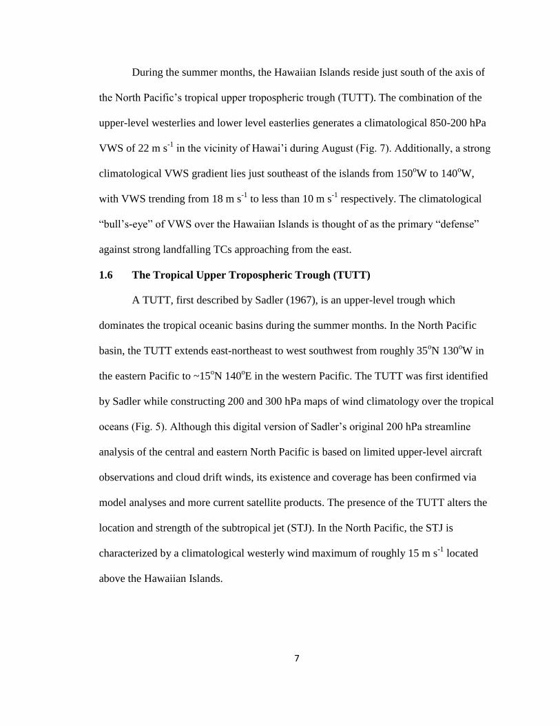
During the summer months, the Hawaiian Islands reside just south of the axis of

the North Pacific’s tropical upper tropospheric trough (TUTT). The combination of the

upper-level westerlies and lower level easterlies generates a climatological 850-200 hPa

VWS of 22 m s-1

in the vicinity of Hawai’i during August (Fig. 7). Additionally, a strong

climatological VWS gradient lies just southeast of the islands from 150oW to 140

oW,

with VWS trending from 18 m s-1

to less than 10 m s-1

respectively. The climatological

“bull’s-eye” of VWS over the Hawaiian Islands is thought of as the primary “defense”

against strong landfalling TCs approaching from the east.

1.6 The Tropical Upper Tropospheric Trough (TUTT)

A TUTT, first described by Sadler (1967), is an upper-level trough which

dominates the tropical oceanic basins during the summer months. In the North Pacific

basin, the TUTT extends east-northeast to west southwest from roughly 35oN 130

oW in

the eastern Pacific to ~15oN 140

oE in the western Pacific. The TUTT was first identified

by Sadler while constructing 200 and 300 hPa maps of wind climatology over the tropical

oceans (Fig. 5). Although this digital version of Sadler’s original 200 hPa streamline

analysis of the central and eastern North Pacific is based on limited upper-level aircraft

observations and cloud drift winds, its existence and coverage has been confirmed via

model analyses and more current satellite products. The presence of the TUTT alters the

location and strength of the subtropical jet (STJ). In the North Pacific, the STJ is

characterized by a climatological westerly wind maximum of roughly 15 m s-1

located

above the Hawaiian Islands.

8

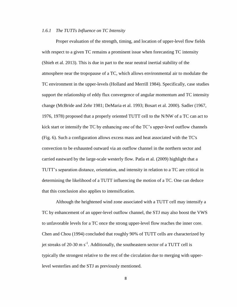
1.6.1 The TUTTs Influence on TC Intensity

Proper evaluation of the strength, timing, and location of upper-level flow fields

with respect to a given TC remains a prominent issue when forecasting TC intensity

(Shieh et al. 2013). This is due in part to the near neutral inertial stability of the

atmosphere near the tropopause of a TC, which allows environmental air to modulate the

TC environment in the upper-levels (Holland and Merrill 1984). Specifically, case studies

support the relationship of eddy flux convergence of angular momentum and TC intensity

change (McBride and Zehr 1981; DeMaria et al. 1993; Bosart et al. 2000). Sadler (1967,

1976, 1978) proposed that a properly oriented TUTT cell to the N/NW of a TC can act to

kick start or intensify the TC by enhancing one of the TC’s upper-level outflow channels

(Fig. 6). Such a configuration allows excess mass and heat associated with the TC's

convection to be exhausted outward via an outflow channel in the northern sector and

carried eastward by the large-scale westerly flow. Patla et al. (2009) highlight that a

TUTT’s separation distance, orientation, and intensity in relation to a TC are critical in

determining the likelihood of a TUTT influencing the motion of a TC. One can deduce

that this conclusion also applies to intensification.

Although the heightened wind zone associated with a TUTT cell may intensify a

TC by enhancement of an upper-level outflow channel, the STJ may also boost the VWS

to unfavorable levels for a TC once the strong upper-level flow reaches the inner core.

Chen and Chou (1994) concluded that roughly 90% of TUTT cells are characterized by

jet streaks of 20-30 m s-1

. Additionally, the southeastern sector of a TUTT cell is

typically the strongest relative to the rest of the circulation due to merging with upper-

level westerlies and the STJ as previously mentioned.

9

1.7 Objectives

According to NOAA’s Hurricane Research Division (HRD), there have only been

four TC-related G-IV deployments in the Pacific basin through 2009, and the G-IV

synoptic surveillance missions conducted around Felicia (2009) were the most

comprehensive. What follows is an investigation of the 65 successful sondes jettisoned

from the G-IV during three consecutive days of synoptic surveillance on 7 to 9 August

2009. This is an unprecedented dataset with regard to in-situ observations around a TC in

the data sparse region of the central and eastern North Pacific. The overall objective is to

shed light on Felicia’s rapid collapse, and determine the value of the G-IV

circumnavigated flight route from an intensity standpoint. Satellite imagery and

reanalysis data will also be used. I examine the following questions, with a focus on the

value of the three consecutive days of G-IV data during the decay of Felicia.

(1) Is there an indication of dry air being imported within the boundary layer or in

the midlevels as evidenced by a combination of the relative radial flow and θe

fields along the 3-degree circumnavigation from 8-9 August?

(2) What is the role of the TUTT as a TC approaches? Is Sadler’s assertion that a

TUTT may contribute to TC intensification exemplified with Felicia?

(3) Can the timing of the STJs intrusion into the inner core of Felicia be determined

based on the winds observed along the circumnavigations performed on

8-9 August? What is the evolution of VWS along the circumnavigation?

10

(4) How successful is the 3-degree circumnavigation at determining factors

contributing to the decay of Felicia? What are the advantages and disadvantages

of utilizing a 3-degree circumnavigation for intensity forecasting?

11

CHAPTER 2

DATA

2.1 Aircraft Utilized and Missions

On 7 August 2009, the NOAA G-IV aircraft departed Long Beach, California to

conduct a 3-day synoptic surveillance of Hurricane Felicia in the eastern North Pacific at

a flight level of 150 hPa. During the ferry out to the Hawaiian Islands on 7 August, the

G-IV deployed GPS sondes to the N and NW of the forecasted cyclone track (Fig. 8). The

duration of the flight on the 7th

was 5.05 h while an average of 6.85 h was invested on 8

and 9 August. On the 8th

and 9th

the G-IV sampled the synoptic environment to the

W/NW of the TC, and then performed a circumnavigational surveillance of Felicia at a

distance approximately 3-degrees latitude from the circulation center (Figs. 9 and 10).

2.2 GPS Dropwindsonde Instrumentation and Deployment

NCAR spearheaded the development and implementation of the GPS sonde. As

highlighted by Hock and Franklin (1999), GPS sonde improvements over the ODW

include global operation at altitudes up to 24 km, simultaneous operation of up to four

sondes per aircraft, a narrow RF transmission bandwidth of < 20 kHz, telemetry range of

325 km, sonde descent time of ~12 min when released from 12 km, sensor measurement

rate of 2 Hz, and a shelf life of at least 3 years (Fig. 11).

The GPS sondes incorporate a Barocap, H-Humicap, and Thermocap for the

pressure, humidity, and temperature sensors, respectively. The Thermocap, developed by

Vaisala, produces a consistent, noticeable response lag in the sondes temperature

measurements that are corrected in the data processing stage. For wind estimates the

sonde has a GPS receiver that records the relative Doppler frequencies from the GPS

12

satellite. These Doppler frequencies describe the motion of the sonde relative to the

satellite. After being digitized, the Doppler frequencies are then sent back to the aircraft

to be converted into winds via the aircraft data system.

GPS sondes are characterized by a 2 Hz sampling rate which translates to a

vertical resolution of 12-14 m at 200-300 hPa and ~5-7 m resolution in the lower

troposphere. In field accuracy is not as accurate as the manufacturer specifications, with

typical errors of pressure, temperature, humidity evaluated at 1.0 hPa, 0.2oC, <5%, and

0.5 m s-1

, respectively. Due to GPS technology, the vertical resolution of wind

measurements are ~6 m, an exceptional advancement from the ODWs ~ 150 m vertical

resolution. Moreover, GPS allows the sonde to measure winds to the surface, whereas

ODW measurements were often missing below 400 m. The accuracy error of the

humidity sensor is an important consideration when analyzing skew-T log-P profiles near

saturation. Sensor wetting, as presented in the following chapter, is also an issue that can

be remediated sometimes by techniques outlined by Bogner et al. (2000) and Barnes

(2008).

Over the course of the 3-day G-IV synoptic surveillance 73 GPS sondes were

deployed with a success rate of 90% (Table 1). This success rate refers to whether or not

vertical atmospheric soundings were achieved at the deployment locations. One aspect of

Table 1 that is particularly noteworthy is that the sondes deployed along the

circumnavigated portion of the flight exhibited a 100% success rate on the 8th

, and 78%

for the 9th

. At first glance this may appear to be a significant disadvantage from an

analysis point-of-view, however the trends around the 9th

circumnavigation are consistent

and an absent sounding can be interpolated from the data obtained by adjacent sondes.

13

2.3 Estimating Sea Surface Temperatures

The Optimum Interpolation (OIV2) SST fields generated by NOAA are used for

the analysis of Felicia. The SST fields are produced weekly on a one-degree grid and

merge buoy, ship, satellite SST data, and SSTs simulated by sea-ice coverage. The root

mean square (RMS) monthly error associated with these SST fields is ~0.8oC. Before the

SST field is completed, the satellite SST fields are adjusted for biases as suggested by

Reynolds (1988) and Reynolds and Marsico (1993). Since the weekly OIV2 SST analysis

is centered on each Wednesday, the week of 5-12 August 2009 is chosen for the SST

analysis of Hurricane Felicia.

2.4 NCEP CFSR Fields

In order to describe the large-scale environment surrounding Felicia when the

G-IV was not in flight, NCEP Climate Forecast System Reanalysis (CFSR) fields are

utilized. This global, high resolution reanalysis product was established in order to

generate the best estimate of the coupled ocean-atmosphere system. CFSR incorporates

all applicable traditional and satellite observations, but with a significantly finer

atmospheric resolution of ~38 km. The G-IV’s GPS sonde TEMPDROPS are included in

CFSR, therefore greater confidence can be placed on the reanalysis fields during the

G-IV sampling periods. CFSR produces a wide variety of variables that are available four

times daily. Specifically, the upper-level wind fields and atmospheric column precipitable

water are employed.

2.5 Satellite Imagery and Satellite Derived Products

Various satellite imagery products are employed before, during, and after the

G-IV sampling periods. Evolution of the Geostationary Operational Environmental

14

Satellites- (GOES) West infrared (IR), visible, and water vapor channels are used to

assess the intensity of Felicia as determined by cloud organization, intensity of

convection, and synoptic flow regimes in the vicinity of Felicia. Observations from

various polar orbiting satellite sensors, particularly the 85 GHz Horizontal channel, are

also utilized to gauge the intensity of Felicia. The 85 GHz frequency band is sensitive to

scattering of radiation by large ice typically found in deep convection. Cooperative

Institute for Meteorological Satellite Studies (CIMSS) satellite imagery overlays and

model analyses are also incorporated. In August 2009, CIMSS employed the Naval

Operational Global Atmospheric Prediction System (NOGAPS) analyses as the

background fields for their local TC analyses. Atmospheric Motion Vector (AMV) fields,

generated by sequences of geostationary satellite imagery, are also incorporated in the

analyses and provide data for observation deficient regions such as the Pacific basin.

15

CHAPTER 3

METHODOLOGY

3.1 Processing of GPS Sonde Data: ASPEN and Beyond

Data from the GPS sondes are first received and processed by the research aircraft

through the onboard Airborne Vertical Atmospheric Profiling System (AVAPS).

Afterwards the data are processed through the Atmospheric Sounding Processing

Environment (ASPEN) program (Martin 2007) which runs the raw AVAPS files through

a series of quality control (QC) algorithms in order to revise or omit unrepresentative

data. ASPEN processes pressure, temperature, humidity, and winds individually. The

winds are decomposed into u and v components. In particular, the ability to compute the

component winds depends on the number of acquired satellites during both the initial

deployment and subsequent descent of each sonde. Overall, inadequate acquisition of

satellites was not an issue during the surveillance of Felicia. The temperature sensor

developed by Vaisala has a lag in the temperature measurements due to the rapid fall

speeds of the GPS sondes at high altitude. ASPEN auto-corrects this temperature lag by

inclusion of the following formula:

t

z

z

TTT m (1)

where Tm is the GPS sonde measured temperature, T/z is the sonde measured lapse

rate, z/t is the sonde measured fall velocity, and τ is the time constant of the

temperature sensor. Additional corrections to temperature and wind sonde measurements

are discussed in Hock and Franklin (1999). ASPEN outputs the AVAPS files in both QC

16

data files and QC skew-T log-P diagrams. A comprehensive overview of the ASPEN

program and its QC procedures are provided by NCAR and Martin (2007) at the

following URL: (https://www.eol.ucar.edu/system/files/Aspen%2520Manual.pdf).

After running the AVAPS datasets through ASPEN, the soundings are

subjectively scrutinized for errors. Although ASPEN is able to resolve most errors

associated with the sondes, issues with sensor wetting, relative humidity (RH) accuracy,

and telemetry require inspection. It is prudent to mention that as the sondes are jettisoned

from the aircraft, there is a time lag in which the pressure, temperature, and humidity

(PTH) sensors equilibrate from the aircraft environment to the atmospheric conditions.

The P and T sensors are able to resolve this equilibration slightly faster than the H-

Humicap. On average, the sondes provide useful data starting at 190 hPa.

Sensor wetting may occur when a sonde passes through a cloud and liquid

collects on the humidity sensor. As a sensor enters into a layer of unsaturated air, the

humidity sensor may continue to read 100% humidity. On a skew-T log-P diagram, a

sensor wetting signature is characterized by a saturated profile along a moist adiabat that

then transitions to a dry adiabatic lapse rate while remaining saturated. Bogner et al.

(2000) offer a simple method to fix sensor wetting; locate where the lapse rate becomes

dry adiabatic while maintaining saturation, and carry a constant mixing ratio from this

level to the surface (Fig. 12). This procedure yields more realistic humidity values for the

subcloud layer which are then used in further analysis.

In the GPS sondes jettisoned around Felicia, some layers of the sonde profiles

hover at >98% RH while following a saturated adiabat. It is reasonable to suspect that

these slight departures from 100% RH are associated with the <5% accuracy error range

17

of the RH sensor. Wang (2005) concluded there is no systematic dry bias of the GPS

sondes RH sensor near saturation. The sondes released around Felicia do not conflict with

this assertion, but it seems reasonable that a dry bias exists within the <5% error range of

the RH sensor with regard to near saturated conditions (Fig. 13). Specifically, if the error

range associated with the RH sensor is <5%, and several sondes depict layers of 98% RH,

how can one refute the possibility that the 2% departure from saturation is not associated

with the inherent accuracy error of the sensor?

Each GPS sonde incorporates a 400 MHz telemetry transmitter in order to send

data from the sonde to the aircraft AVAPS. On a few occasions the telemetry failed,

resulting in layers absent of data. Layers that were thin, and layers that had a very

predictable consistent behavior at start and end points, were interpolated, as described in

the following section.

3.2 Analysis with the Sonde Data

After the sondes undergo case specific error corrections, the successfully

deployed sondes are processed through a program created by Dolling (2012). Felicia

weakened substantially over the three days of sampling, but during each synoptic

surveillance mission of ~6 hours, the TC filled by only a few hPa, so it is reasonable to

assume a steady-state storm for each data gathering period. The duration of the

circumnavigation for the 8th

and 9th

was ~ 2 h. Additionally, the sonde deployments

during the circumnavigation occurred at a radial distance of 3-degrees latitude from the

center of the TC where evolution (e.g., spin down) is likely slower than the core. The

Dolling program outputs a list of variables including but not limited to θe, tangential

18

winds, and radial winds. The following subsections briefly outline the approach of the

program.

The position of each deployed sonde with respect to the movement of Felicia is

essential in order to compute accurate storm relative variables such as radial and

tangential winds. The first step is to formulate the storm track of Felicia. This is done by

decomposing the movement of Felicia into latitude and longitude based on the NHC’s

best track (BT) data. Regression lines were imposed on the center fixes for latitude versus

time and longitude versus time for the 3-day G-IV mission. The circulation center

positions from BT were well approximated by a linear regression with R2> 0.96 for the

G-IV missions.

Once all the GPS sondes are post-processed for erroneous data, a median launch

time for each mission is determined by which all the data during that mission will be

composited. The launch time for each sonde is added to the Dolling program in order to

find the sondes relative time with reference to the composite time of the storm track

during mission. Thus, as the sonde descends its latitude and longitude positions are

deduced with respect to the movement of the storm with time. Every half second time

step in which the GPS sonde takes a reading the pressure, temperature, RH, earth relative

speed of the sonde, direction of the sonde, and altitude is computed with reference to the

relative position of the moving storm. This is conducted for each mission.

Data gaps are caused by an assortment of factors but primarily the data gaps result

from transmission problems and incorrect or failed measurements by the sonde’s

instrumentation. The program that calculates the field variables mentioned above

19

automatically implements linear interpolation of data gaps less than or equal to 300 m.

Gaps larger than 300 m are left as missing data.

3.2.1 Calculating Storm Relative Winds and Thermodynamic Variables

The GPS sonde measures the earth relative speed of the sonde and the direction of

the sonde at half second intervals. To derive storm relative winds, the u and v

components of the storm are subtracted from the u and v components of the GPS sonde at

each time step. The following equations are used to compute the radial and tangential

winds:

Vrad = Urel cos Θ + Vrel sin Θ (2)

Vtan = −Urel sin Θ + Vrel cos Θ (3)

where Urel is the u component of the storm velocity subtracted from the u component of

the GPS sonde and Vrel is the v component of the storm velocity subtracted from the v

component of the GPS sonde. The angle is defined as the angle between the GPS

sonde and a Cartesian coordinate system aligned along a unit circle. Dolling’s program

also computes the vapor pressure, saturation vapor pressure, mixing ratio, specific

humidity, potential temperature (θ), lifting condensation level (LCL) temperature, and θe

based on the procedure outlined by Bolton (1980).

3.2.2 Calculating VWS, Divergence, and Vorticity

Complete vertical soundings in the eastern Pacific basin in proximity to a

powerful TC like Felicia provides the unique opportunity to compute values for VWS.

Both the synoptic environment and the 3-degree circumnavigation around Felicia are

targeted.

20

The VWS is calculated using the following formula:

VWS = √[U225-U850)2 + (V225-V850)

2] (4)

where U225,V225, U850, and V850 are the averaged U and V components of the wind speed

from 200 to 250 hPa (for U225/V225) and 825 to 875 hPa (for U850/V850) as measured by

the GPS sonde. U850 and V850 refer to the U and V components of the wind at 850 hPa.

This 50 hPa average was used in order to get a more representative estimate of the flow

pattern at each level. U225 and V225 were used instead of the traditional level at 200 hPa

because consistent data did not always register near or above 200 hPa. Horizontal

divergence and relative vorticity were calculated using Eqs. (5 and 6) for the area

inscribed by the circumnavigations on the 8th

and 9th

of August. The levels were averaged

+-25 hPa.

𝐷𝐼𝑉 = 𝑑𝑢

𝑑𝑥+

𝑑𝑣

𝑑𝑦 (5)

𝜁 = 𝑑𝑣

𝑑𝑥−

𝑑𝑢

𝑑𝑦 (6)

3.2.3 Circumnavigated Analysis Levels

Throughout this study three layers were analyzed to better understand the collapse

of Felicia, centered at 975, 700, and 250 hPa. These values were chosen to summarize the

influence of adverse factors to Felicia in the subcloud layer, midlevels, and the upper-

levels. The subcloud layer was centered on 975 hPa based upon the circumnavigated

skew-T log-P diagrams representing LCLs of ~950 hPa. For all of the analyses, a 50 hPa

average is computed in order to suppress any outliers and obtain a representative

21

depiction of each layer. Measurements above and below this 50 hPa average were also

investigated for consistency in order to ensure these three levels (975/700/250) are

representative of a deeper layer. For these analyses, we assume Felicia maintains a steady

state as the aircraft conducts the circumnavigations. The time of circumnavigation on 8

August was from 08:40:55-10:59:05 UTC while the sampling period on 9 August

occurred from 09:19:40-11:37:05 UTC.

22

CHAPTER 4

RESULTS

4.1 Formation and Intensification- Attendant Conditions

According to the NHC, Felicia originated in the Atlantic basin on 23 July 2009 as

an easterly wave. This easterly wave moved into the eastern North Pacific and started to

organize deep convection on 1 August around 110oW. The cluster of deep convection

achieved tropical depression (TD) status at 1800 UTC 3 August and tropical storm (TS)

classification 0000 UTC 4 August at approximately 12oN, 122

oW based on both archived

satellite imagery and the NHC’s Tropical Cyclone Report for Hurricane Felicia. With

satellite derived SSTs between 28 and 29oC and a synoptic regime characterized by low

VWS, Felicia rapidly intensified from 0000 UTC 4 August through 0000 UTC 6 August

while being steered to the WNW by a well-defined deep-layer ridge. Felicia achieved a

minimum central pressure of 935 hPa at 0000 UTC 6 August 2009.

Based on NOAA OIV2 SSTs for the week of 6 August 2009 in the eastern North

Pacific basin were .5 to 1.5oC above normal. Consequently, Felicia’s initial growth and

intensification occurred over SSTs greater than 28.5oC near 9

oN 115

oW. As Felicia

tracked toward the WNW and intensified to a category 4 hurricane, SSTs were

maintained at 28-28.5oC. At approximately 1200 UTC 5 August, Felicia started to track

over cooler water. Despite a slight reduction in SSTs, Felicia continued to intensify until

0000 UTC 6 August based on both BT and the Advanced Dvorak Technique (ADT)

intensity estimates.

Felicia developed and intensified along the southern boundary of an expansive,

deep-layered ridge that stretched from the eastern to the central North Pacific. During this

23

period the TC maintained a WNW track at 6-8 m s-1

. On 5 August, Felicia approached the

western boundary of the ridge and entered a weak flow regime characterize by high

pressure far to the NE (Fig. 14). As a result, Felicia’s movement slowed to ~5 m s-1

and

her track shifted due NW from 0000 UTC 5 August through 1200 UTC 7 August. On

7 August, Felicia approached the southeastern quadrant of a rejuvenated high cell and the

dominant flow shifted Felicia’s direction to a more westerly heading again.

The VWS in the immediate vicinity of Felicia during formation and

intensification was fairly weak, on the order of 5-10 m s-1

according to CIMSS model

analysis which incorporates gridded AMV output (Fig. 15). CIMSS VWS analyses

alongside CFSR reanalysis data indicate Felicia remained in a region of low

environmental shear through at least 7 August, however, a strong gradient in VWS

resided more than 5o latitude to the NW of Felicia from as early as 0000 UTC 5 August

onward.

The dry, subsident synoptic regime associated with the Pacific High is clearly

depicted by the average total precipitable water (TPW) during the month of August 2009

as highlighted by the NOAA Special Sensor Microwave Imager Sounder (SSMIS). A

strong zonal gradient in TPW existed from the southern tip of the Baja peninsula to

longitudes near Hawaii; above 20oN, values of monthly averaged TPW were less than

30 mm while the near equatorial convergence zone (NECZ) featured more than 55 mm of

TPW. At 0000 UTC August 7, CFSR depicted TPW values greater than 50 mm covered

an expansive region north of 20oN from 122

oW to 135

oW (Fig. 16). The stark contrast

between monthly averaged TPW and TPW represented at 0000 UTC 7 August 2009 is

attributed to enhanced convection associated with an active NECZ, TS Enrique, and

24

Hurricane Felicia. The dry air signature of the subtropical high is present in Figure 16;

however, the aforementioned convective fields have moistened the atmosphere farther

north than usual. Overall, as Felicia tracked WNW, she entered an increasingly dry

environment with regard to midlevel moisture. This is exemplified by satellite imagery

and overlaid surface pressure analysis as shown in Fig. 17. The influence of this stable

surrounding environment on Felicia’s intensity is evaluated in later sections.

4.2 Actual Intensity versus Maximum Potential Intensity

The actual intensity of Felicia based on BT and ADT is shown in Fig. 18

alongside the estimated central pressure evaluated by MPI theory. During Felicia’s RI

stage, BT and ADT follow closely to each other while the MPI estimation exhibits a low

bias due to its sole evaluation based on surface inflow and tropopause outflow

temperature. At maximum intensity, both the BT and ADT approach the MPI value. It is

important to mention that the deviation between the MPI and BT/ADT at maximum

intensity in Fig. 18 is likely even less since SST was utilized as the inflow temperature

rather than a more representative, slightly cooler near surface inflow temperature. Felicia

began to lose intensity at 0600 UTC 6 August. During this time all three curves

(BT/ADT/MPI) exhibit an equivalent weakening trend through 0600 UTC 7 August. This

initial decay reflects the decrease in inflow temperature as Felicia tracked over cooler

SSTs. At 0600 UTC 7 August the three curves diverge, with BT maintaining a gradual

weakening trend, ADT suggesting enhanced weakening, and MPI leveling off. At

1800 UTC 7 August, ADT indicates a re-intensification through 0600 UTC 8 August

with BT suggesting continued weakening. At 1200 UTC 8 August, ADT begins to

suggest a weakening trend and catches up to BT at 0000 UTC 9 August.

25

4.3 SSTs and the Initial Decay

From 0000 UTC 6 August through 0000 UTC 8 August Felicia tracked toward the

NW, across strong SST gradients; SSTs decreased from 28.5oC to below 25.5

oC

underneath the circulation center (Fig. 19). Correspondingly, minimum sea level pressure

filled from 935 to 970 hPa according to BT. This SST decline is supported by the fact

that the BT and ADT intensity estimates follow the same trend as MPI from 0600 UTC 6

August through 0600 UTC 7 August. On 8 August, SSTs stabilized at 25-25.5oC beneath

the storm center as Felicia moved due W.

4.4 Outflow Channel Enhancement

After Felicia tracked over cooler waters from 0600 UTC 6 August through 1800

UTC 7 August (Fig. 19), Felicia re-intensified as highlighted by CIMSS ADT, the

Tropical Analysis Forecast Branch (TAFB), and the NHC’s Hurricane Felicia Discussion

at 0300 UTC 8 August. According to CIMSS ADT, the estimated central pressure

dropped from 980 hPa to less than 960 hPa between 1800 UTC 7 August and 0000 UTC

8 August (Fig. 18). Interestingly, the NHC BT maintained a steady weakening trend

during this period. At 0000 UTC 8 August, NHC BT evaluated Felicia’s central pressure

at 970 hPa while TAFB estimated a central pressure of 960 hPa. Figure 20 shows four

satellite IR views every 3 h during the re-intensification from 1500 UTC 7 August

through 0000 UTC 8 August. Note that the spatial extent of the cold cloud tops less than

-50oC increased, these cold tops became more axisymmetric, and the eye also became

better defined. Tropical Rainfall Measuring Mission (TRMM) 85 GHz Horizontal

imagery also portrayed a period of re-intensification, with better organization of deep

convection around the eyewall between overpasses at 1354 UTC and 2205 UTC 7

26

August. According to CIMSS, Felicia began filling at 0600 UTC 8 August. At this time,

the estimated pressure difference between BT and ADT was more than 15 hPa.

Unfortunately, C-130 aircraft reconnaissance was not helpful in pinpointing a central

pressure during this re-intensification since the earliest mission occurred at 1400 UTC 8

August. The preponderance of evidence supports the contention that Felicia did re-

intensify though 20 hPa may be viewed as somewhat extreme deepening.

4.4.1 Is the STJ Responsible for Felicia’s Re-Intensification?

Black and Anthes (1971) used satellite derived winds to determine that the major

outflow channel winds of mature TCs extended to an average radius of 800 km. Since

Felicia was not a major hurricane prior to re-intensification as evidenced in Fig. 20a, an

anticyclonic outflow of 8 degrees latitude is not likely. In fact, during Felicia’s re-

intensification water vapor and visible satellite imagery indicated Felicia’s anticyclonic

circulation extended outward to about 4.5 degrees latitude (or ~500 km) within the NW

quadrant (Fig. 21). In another applicable study, Sadler (1976) examined the interaction

between TUTTs and nascent typhoons Gilda and Harriet. Sadler noted that an interaction

appeared to occur when the TUTT was approximately 500 km from the nascent TC’s

surface vortex. Felicia was an established TC prior to interaction with the TUTT;

therefore a distance of 500 km between the TUTT and the vortex center of Felicia is

likely associated with heightened VWS rather than beneficial outflow enhancement.

In order to evaluate if Felicia’s re-intensification was attributed to an enhanced

outflow channel, as shown for other TCs by Sadler (1976, 1978), the upper-level flow

field and its relationship to Felicia’s anticyclonic outflow channel are examined. A

stronger outflow channel removes low momentum from the core and thus acts as a

27

momentum source (Holland and Merrill 1984). GOES West water vapor imagery and

overlain Global Forecast System (GFS) model 250 hPa heights and winds shed some

light on the potential interaction between the TUTT’s attendant STJ and the outflow

channel of Felicia (Fig. 22). Initially, the STJ and its associated wind field are positioned

more than 800 km to the NW of Felicia’s anticyclonic outflow (~4.5 degrees latitude

from the core of Felicia). As the separation distance between the STJ and the outflow

channel decreases, at some point the anticyclonic outflow of Felicia is given a boost via

the complementary wind flow associated with the STJ. In order to quantify the degree of

interaction, a separation distance is determined, defined as the distance between Felicia’s

anticyclonic outflow at 4.5 degrees and the gradient of 15-18 m s

-1 winds at 250 hPa

based on CFSR. It is important to reiterate that the 7 August G-IV GPS sonde data is

incorporated into the CFSR fields, therefore greater confidence can be placed on the

position and strength of the STJ during the period of G-IV surveillance. The G-IV data

was not used exclusively in determining the separation distance because the 7 August

G-IV flight was not a comprehensive synoptic surveillance mission like 8 and 9 August.

An example of the methodology in determining the separation distance is demonstrated in

Fig. 23.

The results indicate that separation distance (defined in prior paragraph) steadily

decreases from ~700 km at 0000 UTC 7 August to zero km at 1200 UTC 9 August (Fig.

24). During Felicia’s re-intensification from 1800 UTC 7 August through 0600 UTC 8

August, separation distance drops from roughly 400 to ~230 km. After this point the

separation distance continues to steadily drop to zero. The evolution of this separation

distance analysis indicates that there is a period in which the STJ may have provided an

28

enhanced outflow channel for Felicia to re-intensify. Specifically, this distance is 400 to

230 km from the TUTT’s STJ to the anticyclonic outflow of Felicia, or roughly 900 to

730 km from the STJ to the vortex center of Felicia. Since SSTs are on the decline and

Felicia entered an environment of lower midlevel moisture, it is reasonable to posit that

the re-intensification of Felicia is possibly due to enhancement of the northern

anticyclonic outflow channel. This conclusion is supported by satellite imagery, CIMSS

ADT, and NHC Hurricane Felicia advisory discussions.

4.5 Basic G-IV Analyses

At the time of Felicia’s re-intensification, the G-IV was en route to Honolulu and

sampling the environment to the N and NW of Felicia. GPS sondes were jettisoned along

the flight route from 5:30-13:30 UTC 7 August. All deployed sondes described an

environment associated with the Pacific High: deep-layered easterly flow with strong

inversions in the east transitioning to higher, slightly weaker inversions at longitudes near

the Hawaiian Islands. The deep layer of low relative humidity and the near dry adiabatic

lapse rates above a strong inversion are indicative of subsidence. Specifically,

deployment location #1 had an inversion base of ~950 hPa while sonde deployments

10-17 had inversions around 800 hPa. On 7 August, the axis of the TUTT at 200 hPa

extended from NE to SW at longitudes of 150-155oW. Elsewhere, west-southwesterly

flow dominated above 300 hPa associated with the STJ. Below 300 hPa, easterly flow

prevailed.

Before and after the G-IV completed a circumnavigated route around Felicia on 8

and 9 August, the aircraft conducted synoptic surveillance of the environment to the NW

of Felicia. Similar to the 7th

, the skew-T log-P diagrams in the environment to the NW of

29

Felicia on the 8th

and 9th

suggest subsidence, and inversions reside at ~825 hPa. As one

might expect, deployment location #8 on 8 August described an environment in transition

between the synoptic environment and that of Felicia; a weaker inversion and higher

boundary layer moisture content. At the 3-degree circumnavigation, higher moisture

resided throughout the depth of the troposphere (Fig. 25). The green vertical profile of θe

portrays the layer averaged environment based on sonde deployments 1-7 and 24-27 (Fig.

9) and 1-11 and 26-27 (Fig. 10). Therefore, this green curve represents a typical θe profile

one might expect in the Tradewind environment; modest θe values in the low-levels

dropping to a low mid-tropospheric minimum at 775 hPa followed by a gradual increase

to the top of the troposphere. Although both the 8th

and 9th

circumnavigation profiles are

similar in overall structure, on average, the 300-800 hPa θe layer on the 8th

is ~3 K greater

than the 9th

highlighting a decreasing trend in θe around the 3-degree circumnavigation

between the sampling periods on 8 and 9 of August.

Divergence and vorticity are calculated for the circumnavigation at 8:40-11:00

UTC 8 August and 9:20-11:40 UTC 9 August. The layered analysis of divergence

exhibits convergence below 800 hPa, with 8 August demonstrating slightly greater

convergence throughout this layer with a peak value at -2.4 x 10-5

s-1

(Fig. 26). Above

800 hPa and continuing to ~200 hPa on 8 August there is weak divergence. Contrarily,

from 200–400 hPa, 9 August analysis portrays strong convergence with a maximum near

200 hPa at -2.15 x 10-5

s-1

. This convergence aloft is attributed to the nearby STJ and its

SW flow impinging on the 3-degree ring. The low resolution of this layered analysis of

divergence suggests there may be convergence from the STJ at levels as low as 600 hPa;

30

however, storm relative wind flow indicates the STJ’s wind field does not penetrate

below 400 hPa.

Vorticity for the circumnavigations paints a predictable picture of positive relative

vorticity throughout the depth of the analysis, and a trend towards zero at 200 hPa (Fig.

27). With relative vorticity essentially zero at ~200 hPa, it can be deduced that this

3-degree circumnavigational ring occurs proximate to the inflection point in which the

cyclonic nature of Felicia transitions to anticyclonic outflow. The largest values of

relative vorticity for the 8th

and 9th

are 7.0 x 10-5

s-1

and 6.6 x 10-5

s-1

respectively, and

occur at near 800 hPa. This trend from 8 to 9 August corresponds to a reduction of

relative vorticity by ~ 6%.

4.6 Subcloud Layer Fields

In order to investigate the detrimental effects, if any, residing in the boundary

layer, composites of both storm relative flow fields and θe are examined along the 3-

degree circumnavigations within the subcloud layer. On average, skew-T profiles from

the GPS sondes revealed a cloud base of roughly 950 hPa therefore this subcloud layer

analysis was centered at 975 hPa. Based on the tangential flow at 975 hPa, both 8 and

9 August indicate a highly asymmetric wind field at 3-degrees (Fig. 28a). The strongest

tangential winds on both days are ~15 m s-1

, with a peak in the W quadrant on 8 August,

transitioning to the N on 9 August. The weakest tangential winds lie clockwise from N to

S on 8 August at ~9 m s-1

while 9 August is characterized by minimum winds in the E/SE

quadrant at ~5 m s-1

. From the 8th

to the 9th

, the average tangential flow around the

circumnavigation drops from over 11 m s-1

to less than 9 m s-1

suggesting a drop of

intensity between the 8 and 9 August sampling periods. The storm relative radial flow

31

paints a similar picture of asymmetry; radial inflow peaks along the N to NE sector for

the 8th

and from the N to E quadrant on the 9th

(Fig. 28b). Interestingly, there is greater

inflow on the 9th

, at more than -10 m s-1

as compared to ~-8 m s-1

on the 8th

. From 8 to 9

August, weak inflow in the S/SW sector transitions to outflow.

The θe values at 975 hPa range from 340 to 350 K along both of the 3-degree

circumnavigations (Fig 29). Both 8 and 9 August profiles are similar except for a marked

decrease in θe along the NNW-NNE quadrant on the 8th

. This minimum in θe along the N

quadrant is collocated with storm relative radial inflow of -6 to -8 m s-1

. These θe values

of 340 K in the N/NW sector of the circumnavigation on the 8th

are quite similar to the θe

values of the synoptic environment on 8 and 9 August suggesting the N/NW section of

the circumnavigation on 8 August is representative of trade wind air.

IR satellite imagery at 0900 UTC 8 August demonstrates that most of the

deployment locations, including the N/NW sector, were located outside of the primary

convection associated with Felicia (Fig. 30). In this figure, the red circle denotes a radial

distance of 3-degrees latitude from Felicia’s center of circulation and the approximate

location of the deployed sondes. What is evident is that in the northern sector this red line

resides along the boundary between Felicia’s cirrus outflow and the stratocumulus field

associated with the Subtropical High. Therefore, the minimum in θe during the

circumnavigation on the 8th

is most likely due to a gentle intrusion of environmental air.

In order to determine if this drop in θe at 3-degrees along the N/NW sector is responsible

for the weakening of Felicia, a theoretical air parcel is timed from this radial distance to

the inner core. A few assumptions need mention; firstly, this estimation assumes that the

analysis at the 975 hPa level applies to the majority of the subcloud layer. Secondly,

32

moisture and heat fluxes in the boundary layer are not considered, partially because

AXBTs were not jettisoned during reconnaissance of Felicia. Finally, the radial flow is

assumed to increase linearly to -12 m s-1

as the parcel travels radially inward to the core.

With these assumptions in mind, storm relative radial flow increasing from -7 to -12 m s-1

with decreasing radius would take roughly 8-9 h to reach the core of Felicia given the

observation at a radial distance of 3-degrees. If the near core radial inflow was -15 m s-1

,

the flow along the 3-degree ring would reach the core in ~7.5 h. The timing of these

potential intrusions into Felicia’s core are in alignment with the decrease in Felicia’s

intensity observed from 8-9 August, however, it is important to note that this minimum in

θe is not present in the θe profile for the 9th

, suggesting that the decrease in the θe on the

8th

is not a prolonged feature during the sampling periods. Moreover, the three sondes

that measured substantially lower values of θe on 8 August account for only 21% of the 3-

degree ring. Although the aforementioned assumptions are constraining, especially the

diabatic effects associated with ~7.5 h of residence time in Felicia’s inner region, this

estimation demonstrates the influence of dry air in the subcloud layer was not significant.

C-130 aircraft reconnaissance flights into the core of Felicia on 8 and 9 August

were able to determine if the lower θe values observed along the N/NW sector of the

G-IV’s 3-degree circumnavigation on 8 August influenced Felicia’s intensity. The C-130

flight on the 8th

began at 14:45 UTC 8 August and ended at 00:39 UTC 9 August while

the flight on the 9th

took place from 02:28 UTC to 12:08 UTC 9 August. Four center fixes

were obtained on each mission. Between the last center fix on the 8th

and the first center

fix on the 9th

, a 6 h period, the central pressure of Felicia rose approximately 2 hPa. From

the 8th

to the 9th

, averaged θe profiles in the subcloud layer for sondes jettisoned in the

33

near eyewall region exhibited a drop of 1.5 K. A drop of 1.5 K translates to an estimated

increase in a TC’s central pressure of 4.5 hPa (Malkus and Riehl 1960; Emanuel 1986).

Since only 2 hPa of filling was observed from the C-130 center fixes, the decay was even

slower than observational studies suggest (i.e., the eyewall column did not degrade as

much as the assumption that -1.5 K extends throughout the column). Therefore, these

C-130 missions demonstrate that the lower θe air measured along the G-IV’s 3-degree

circumnavigation on the 8th

did not substantially impact the central pressure of Felicia.

4.7 Evidence of Dry Air Entrainment in the Midlevels

The storm relative radial flow in unison with θe at 700 hPa is analyzed with the

primary objective to determine the presence and possible impact of drier, midlevel air at

the 3-degree circumnavigations (Fig. 31). The storm relative radial flow (Fig. 31a)

demonstrates a similar profile for both 8 and 9 August; peak radial outflow of ~5 m s-1

in

the W-NW sector is followed by a gradual decline to very weak radial inflow of -1 to

-2 m s-1

in the NE through SW portions of the circumnavigation. Figure 31b highlights θe

values in the midlevels. Clockwise from SW to NE, both 8 and 9 August indicated that θe

fluctuates between 335 K and 342 K. In particular, the SE quadrant exhibited a drastic

decrease in θe during both sampling periods, with the 8th

dropping to 330 K and 325 K on

the 9th

. This sector of lower θe was collocated with very weak storm relative radial inflow

of -1 to -2 m s-1

on both circumnavigations. This very weak 700 hPa radial inflow at a

radial distance of 3-degrees is supportive of vertical profiles of radial flow composed by

Frank (1977). With the assumptions outlined in the previous section in mind, this sector

of lower θe on the 8th

would have reached Felicia’s core in 1.7 days, a value far too long

to be a noticeable factor in Felicia’s decay since Felicia’s central pressure began to

34

steadily fill at approximately 1800 UTC 8 August. With this time estimation, I have

assumed that there is no increase in the radial flow through the midlevels, unlike the

subcloud layer. This signature of lower θe in the midlevels at 3-degrees is more

representative of environmental air, as previously highlighted in Figure 30. Comparison

to visible and IR satellite imagery during the sampling period supports the contention that

the GPS deployments occurred along the fringes of the cloud mass associated with

Felicia.

4.8 Evidence of the STJ’s Intrusion into the Inner Core

The strength and position of the STJ with respect to Felicia was critical in

determining the degree of influence on Felicia’s intensity. At 0900-1240 UTC 7 August,

the TUTT axis resided at approximately 25oN 152.5

oW with 25 m s

-1 winds draped from

147.5oW to 140

oW at 26

oN (Fig. 32a). During this time frame, the approximate position

of Felicia’s center of circulation was 18oN 135

oW. On 8 August the TUTT, which alters

the strength and location of the STJ, retrograded, and the strongest winds were located

just NE of the Hawaiian Islands at 22.5oN 152.5

oW (Fig 32b). Figure 32c demonstrates

that the STJ followed the motion of the TUTT and established itself over the Hawaiian

Islands. Furthermore, the STJ increased its coverage and strength from 8-9 August,

becoming more zonal and expanding its area of high winds along longitudes near Hawaii,

and just east of 150oW.

Latitude-longitude plots presenting only the GPS recorded storm relative winds

allow one to explicitly determine the degree of influence of the STJ on the 3-degree

circumnavigated ring. The 3-degree circumnavigation on 8 August (Fig. 33a) was

characterized by much weaker winds in comparison to the 9th

(Fig. 33b). Along the NW

35

and SW quadrants on the 8th

winds were ~5 m s-1

, with anticyclonic flow along the NW

sector and cyclonic flow to the SW. Contrarily, the storm relative winds on 9 August had

a westerly component throughout the circumnavigation, with over 15 m s-1

westerly

winds where the STJ impinged on Felicia. Overall, the storm relative flow at 200 hPa

illustrates the intrusion of westerly flow associated with the STJ; the west side of the

circumnavigation had strong W winds while more variable winds, in both magnitude and

direction, characterized the eastern half. Since the E side of the circumnavigation was

further away from the STJ and blocked by Felicia’s vortex structure the winds were,

unsurprisingly, weaker. However, the winds still exhibited a westerly component on the

E side of the circumnavigation, suggesting that the STJ’s adverse winds had reached the

core of Felicia by the time of the sampling on 9 August.

From 8 to 9 August, both the storm relative tangential and radial flows at 250 hPa

demonstrated increasing interaction with the TUTT’s STJ (Fig. 34). On 8 August,

tangential flow was weak throughout the majority of the circumnavigation. Tangential

flow on the 9th

was substantially different; strong cyclonic flow was limited to the SW

portion of the circumnavigation, rapidly shifting to anticyclonic flow along the NW

sector due to the proximity of the STJ. This pattern suggests a zone of strong divergence

in the west due to the influence of the STJ. The storm relative radial flow at 250 hPa

portrays a clear picture; intrusion of the TUTT’s attendant STJ is evident at the 3-degree

circumnavigation (Fig. 34b). Specifically, the 8th

was characterized by radial inflow in

the W-NW sector of -3 to -4 m s-1

while 9 August was over -20 m s-1

.

Since the amount of moisture at 250 hPa is minimal, analysis of θe is comparable

to θ. The θe values along the circumnavigation at 250 hPa indicate the intrusion of the

36

STJ was not accompanied by a substantial change in θe, or θ for that matter (Fig. 35). As

shown, θe on both 8 and 9 August only ranges from 345.5 to 348 K. In fact, data suggests

that the intrusion of the jet along the NW sector is associated with a modest increase in θe

of roughly 2 K.

4.8.1 Quantifying the STJ’s Intrusion into the Inner Core

The VWS from 850-225 hPa further substantiates the adverse impacts of the STJ

(Fig. 36). Along the 3-degree circumnavigation, 8 August exhibited wind shear of

8-15 m s-1

throughout the circumnavigation while 9 August demonstrated a doubling of

the VWS in the NW quadrant to more than 30 m s-1

. Therefore, it is clear that the STJ

intruded into the 3-degree ring along the W-N quadrant while the easternmost extent was

somewhat sheltered and remained at less than 15 m s-1

VWS. There is less than 5 m s-1

VWS in the SW quadrant on the 9th

, a location just S of the influence of the STJ.

The radial flow at 250 hPa rose substantially between the sampling period on

8 August to the sampling period on 9 August; gentle inflow of -3 to -4 m s-1

was replaced

by -20 m s-1

of radial inflow in the W/NW quadrant. Based upon satellite imagery at

1200 UTC 9 August, the upper and lower level circulations of Felicia were already

separated by the end of the G-IV sampling period at 11:40 UTC 9 August (Fig. 37). This

separation is represented by colder cloud tops of the upper-level circulation being

displaced to the east and the lower level circulation exposed to the west with warmer

cloud tops.

Since both satellite imagery and GPS sonde analyses suggest that the STJ had

already intruded into Felicia’s core before the end of the G-IV surveillance on the 9th

, the

250 hPa radial inflow along the NW quadrant was linearly interpolated between the

37

observation periods on 8 and 9 August, resulting in a value of -10 to -12 m s-1

radial

inflow at 0000 UTC 9 August. With the eyewall radius evaluated at 50 km, -11 m s-1

radial inflow in the NW quadrant would have reached Felicia’s core in approximately

7 h. This eyewall radius of 50 km is based upon the NOAA HRD 9 August H*wind

analysis following the scheme developed by Powell et al. (1998), which incorporates the

C-130 aircraft data and all other available observations platforms. The radial inflow was

estimated from the 3-degree circumnavigation to the eyewall. The timing of this radial

inflow estimated intrusion (0700 UTC 9 August) corresponding with IR satellite imagery

is shown in Fig. 38. In this figure, deep convection associated with Felicia is graphically

represented by the spatial extent of IR estimated cloud tops with temperatures less than -

50o C. As shown, coverage of deep convection is 3-4 degrees

2 until 0600-0700 UTC 9

August, at which point deep convection (T < -50o C) steadily drops to zero. Satellite

imagery evidence, demonstrating the initial stages of the STJ’s flow impinging on the

eyewall of Felicia with the upper-level circulation and deepest convection being

displaced downshear to the east and northeast is shown in Fig. 39a. Figure 39b is a visible

image of Felicia at 1600 UTC 9 August, with the low-level circulation clearly discernable

along the western portion of the satellite image and downshear displaced convection

straddling the east side of the vortex.

4.9 SHIPS Shear Evaluation of Felicia

The SHIPS operational forecasted shear is a blended calculation from the SHIPS

shear predictors, SHDC and SHGC. Both SHDC and SHGC are computed from GFS

model data and are evaluated from 850-200 hPa with an annulus of 0-500 km relative to

the 850 hPa vortex center, after which the GFS model vortex is removed. SHGC is the

38

generalized shear, and differs from SHDC in that its shear value is computed by a

pressure integral from 850 to 200 hPa rather than the two level of 850 and 200 hPa. The

G-IV datasets on 8 and 9 August were absorbed into the SHIPS 1200 UTC GFS model

runs, therefore these model runs have the added benefit of in-situ measurements in the

vicinity of Felicia in order to better represent the true environmental flow, and

subsequently, VWS.

Figure 40 presents the SHIPS operational forecasted shear after maximum

intensity at 0600 UTC 6 August. Also plotted are the averaged 850-225 hPa storm

relative VWS values around the G-IV 3-degree circumnavigations on 8 and 9 August.

While the SHIPS shear predictors determine a shear value for an area 0-500 km relative

to the 850 hPa vortex center, the storm relative G-IV computations of shear are solely

determined by taking an average of the shear values along the 3-degree

circumnavigations. Since the values of shear are not computed in the same fashion, there

are large differences between the SHIPS shear forecast trends and the shear calculated

from the circumnavigated GPS sondes. With consideration to this difference in shear

methodology, the timing of the shear increase is more comparable than the variation in

shear magnitude. Somewhat surprising, the SHIPS forecast on 6 August demonstrated the

closest trend with regard to the timing of increasing shear; SHIPS shear forecasts on 7

and 8 August suggested a reduction in shear around Felicia from 1200 UTC 8 August to

0000 UTC 9 August while both the SHIPS 6 August forecast and the trend in G-IV

circumnavigations from 8 to 9 August portrayed an increasing trend.

39

CHAPTER 5

CONCLUSIONS AND FUTURE WORK

5.1 Summary and Discussion

Hurricane Felicia was a major hurricane in the eastern and central North Pacific

basin that threatened the Hawaiian Islands. Felicia reached a peak intensity of 935 hPa at

0000-0600 UTC 6 August. Beginning 7 August, the NOAA G-IV aircraft conducted

synoptic surveillance of Felicia with the primary interest to improve forecasts of its track.

During 8 and 9 August, the synoptic environment in which the TC was intended to track

towards was sampled, and then a circumnavigation around the TC was conducted at a

radial distance of 3-degrees latitude. The timing of each surveillance mission provided

the opportunity to analyze an often overlooked stage of a TC’s life cycle, decay. The

value of this 3-degree circumnavigation from an intensity perspective was also examined.

The primary caveat of this study is that the original intention of the G-IV deployment

distributions was to improve track forecasts not intensity, therefore overt data gaps exist.

Additionally, the circumnavigations are unable to recognize any processes in the core of

Felicia such as eyewall replacement cycles, eyewall contraction, eye to eyewall mixing,

convective flare-ups in the eyewall, and rainband competition within the eyewall.

Felicia’s best track overlaid on the weekly satellite derived SST field indicated

that Felicia moved over strong SST gradients just after maximum intensity. Specifically,

SSTs dropped from 28.5oC to below 25.5

oC underneath the circulation center from 0000

UTC 6 August through 0000 UTC 8 August coincident with the initial filling of Felicia’s

central pressure. During this time frame the synoptic environment to the N and NW of

Felicia, as evidenced by satellite imagery and the GPS sondes, revealed deep layered

40

easterly flow emanating from the semi-permanent Pacific High. These easterlies were

characterized by low relative humidity and near dry adiabatic lapse rates above strong

inversions, suggestive of stable, subsident flow. Since the evolution of Felicia’s MPI

curve followed the same slope as the intensity estimations of BT and CIMSS ADT, it is

reasonable to conclude that reduction of SSTs was the first blow to Felicia’s intensity.

After a drop in intensity attributed to SSTs, the most critical component with

regard to Felicia’s intensity was the evolution of the STJ lying to the NW of Felicia and

the westward movement of the TC. Above ~300 hPa, west-southwesterly flow prevailed,

associated with the STJ. The upper-level trough, synonymous with the TUTT, and the

STJ slowly retrograded from its position on 7 August at ~25oN, 150-155

oW. As Felicia

tracked due W, the separation distance between Felicia’s outflow channel and the

gradient of strong winds associated with the STJ decreased from ~700 to 400 km. During

Felicia’s re-intensification of ~20 hPa as evidenced by CIMSS ADT, this separation

distance declined from 400 to 230 km. Therefore, as Felicia tracked westward towards

the upper-level jet there was a transition from little to no interaction with Felicia, to a

short-lived period of anticyclonic outflow enhancement at large radii, and then an

overwhelming impingement of the STJ on the core of Felicia on 9 August. Since Felicia

entered an increasingly hostile environment with regard to SSTs and a stable synoptic

regime, it is reasonable to conclude that the re-intensification was attributed to a brief but

optimal separation distance and orientation between the STJ and Felicia’s northern

anticyclonic outflow. These results are supportive of the pioneering work of Sadler

(1967, 1976).

41

The G-IV circumnavigations during Felicia’s decay on the 8 and 9 August

revealed that, in both the subcloud layer and midlevels, there was no convincing evidence

of lower θe air being entrained into the inner core of Felicia. The observed drop in θe on 8

August in the N/NW sector of the subcloud layer was characterized by substantial radial

inflow, however, due to the duration and distance of the inflow trajectory from this

confined portion of the circumnavigation to the core of Felicia it is reasonable to

conclude that this measured drop in θe on the 8th

was not a pivotal factor in Felicia’s

decay. Moreover, the subcloud layer on the 9th

revealed that the observed drop in θe along

the N/NW sector of the circumnavigation on 8 August had recovered. The midlevel drop

in θe observed on both 8 and 9 August in the SE sector were not associated with inflow

rates larger than -2 m s-1

, therefore this midlevel flow is also not a factor in Felicia’s

collapse.

In contrast, the upper-levels painted a clear picture with progressive intrusion of

the STJ from 8 to 9 August. Specifically, the radial inflow along the NW sector of the

circumnavigation quintupled from less than -4 m s-1

on 8 August to more than -20 m s-1

on 9 August. One may have expected that such a strong advection of environmental air

into the inner core to be accompanied by a change in θe (a proxy for θ or temperature at

such high altitudes). However, results indicated a flat θe profile characterized the NW

sector from 8-9 August. With corresponding satellite imagery exemplifying the effects of

VWS, the demise of Felicia was ultimately attributed to the debilitating effects of deep

layer wind shear in excess of over 30 m s-1

impinging on the W/NW sector of Felicia.

Although satellite imagery and GPS sonde computed VWS clearly highlight the

impact of VWS on Felicia, the physical mechanisms by which VWS acts to weaken a

42

mature TC are more ambiguous. While the theory of ventilation (Simpson and Riehl

1958; Gray 1968), in which a sheared environment displaces upper tropospheric warm

anomalies from the low-level convergence of heat and moisture is widely accepted as a

debilitating factor for developing TCs, the exact physical mechanism of how this occurs

is still uncertain. DeMaria (1996) points out that ventilation of a mature TC, where warm

air is drawn away from the upper-levels, would tend to de-stabilize the inner core of a TC

and promote intensification. Additionally, ventilation may transport away low

momentum air residing in the upper troposphere leading to enhanced flow over the inner

core. This transport acts as a momentum source, and potentially contributes to spin-up of

the vortex (Holland and Merrill 1984). From a thermodynamic perspective, ventilation of

the warm core itself would lead to a temperature-pressure-wind adjustment; the addition

of cooler, drier air would act to reduce the pressure gradient, weaken the surface winds,

and consequently lower the energy fluxes drawn from the sea surface.

While the ventilation of a mature TC may act to increase or decrease the central

pressure, conceptual models of the tilting of a TC core are widely recognized to adversely

affect intensity. The vertical integration of the warm air in the eye and eyewall column of

a tilted core highlights the weakening effects of TC tilt; reduced limits of integration for a

tilted core results in a thinner layer of integrated warm air, which leads to a rise in sea

level pressure, a weakening of the pressure gradient, reduced surface wind speeds, and

less energy fluxes drawn from the sea surface.

DeMaria (1996) used a simple two-layer model to show that the potential vorticity

(PV) of the vortex becomes tilted in the vertical when the upper-level vortex is displaced

from the lower layer. In order to maintain a mass balance, the model vortex responds to

43

this PV tilt by inducing a midlevel warm perturbation above the low-level circulation

center. In an actual TC, vertical stability associated with midlevel warming would act to

inhibit core convection and lead to a filling of the central pressure. Additionally, this two-

layer model of PV tilt also produced a cold anomaly downshear of the low-level vortex

center that would promote convection in this downshear region. Firstly, this downshear

convection would tend to rob the eyewall convection of inflow energy. Secondly, the

downshear convection may generate downdrafts and outflow boundaries that would

replace the inflow layer with lower θe air, leading to a reduction of moist enthalpy

available to the eyewall. Therefore, this sequence of events combines the shear arguments

discussed by Riemer (2010) and the adverse impacts of downdrafts pioneered by Barnes

et al. (1983) and Powell (1990).

The numerical simulations produced by Frank and Ritchie (2001) suggest that

weakening evolves from the top down. Essentially, they concluded that shear generates

asymmetric upper-level PV and θe fields along with the deterioration of the upper-level

warm core structure, which induces a rise in surface pressure. Frank and Ritchie (2001)

hypothesize that the low inertial stability in the upper-levels allows the shear to prescribe

these asymmetric patterns to the upper-levels first, before shifting downward with time

and producing an increasingly shallower, vertically aligned.

How did shear lead to the demise of Hurricane Felicia? First, the satellite

presentation of Felicia demonstrates a distinct downshear displacement of deep

convection and this observation is supported by most conceptual models and

observational studies (Black et al. 2002). While this supports the conclusions of both

DeMaria (1996) and Frank and Ritchie (2001), the mechanisms of the two studies are

44

vastly different. Although both DeMaria (1996) and Frank and Ritchie (2001) stress the

importance of asymmetries, the mechanisms and sequence of events by which a warm

core dissipates in a sheared flow are not well understood. The low inertial stability in the

upper-levels as presented by Holland and Merrill (1984) leads me to believe the initial

weakening mechanism begins in the upper-levels. With regard to Felicia, I hypothesize

that the heightened VWS acted to tilt the upper-level core downshear as well as disrupt

the concentrated PV and θe fields of this layer. While the agitation of these PV and θe

fields reorganize the vertically aligned vortex from the top down, the tilted core and

asymmetries promote a downshear displacement of deep convection. The outflows from

the downshear convection advect upshear and stabilize that region, further enhancing

asymmetries. The shift in deep convection from the eyewall region to the downshear

region at greater radii disrupts the original circulation in the lower levels by rerouting a

portion of the inflow layer to the new downshear convection. More robust observation-

based missions may be able to map the evolution of these conceptual models in order to

pinpoint the most important mechanisms involved in how a warm core dissipates in a

sheared environment.

The timing of the STJ’s NW impingement on Felicia’s eyewall was quantified

using a linear interpolation of the storm relative radial flow along the 3-degree

circumnavigation. Although several assumptions were implemented, -10 to -12 m s-1

of

radial inflow translated to an intrusion 7-8.5 hrs later. This estimated intrusion was well

supported by IR satellite imagery demonstrating the initial stages of the upper and low-

level circulations undergoing separation and collapse of vigorous convection around the

western half of the eyewall.

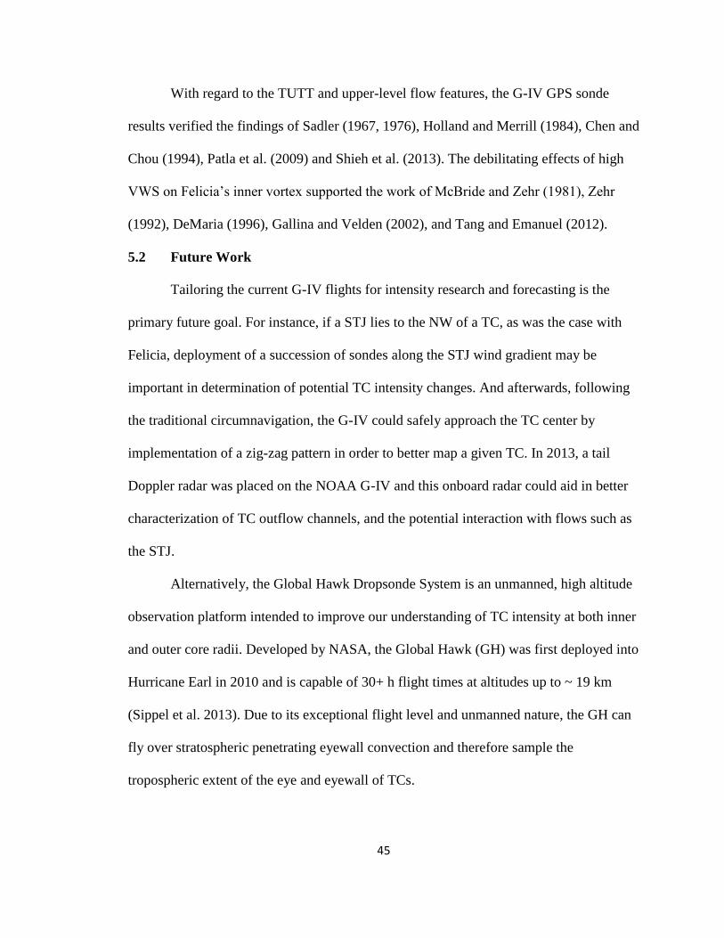
45

With regard to the TUTT and upper-level flow features, the G-IV GPS sonde

results verified the findings of Sadler (1967, 1976), Holland and Merrill (1984), Chen and

Chou (1994), Patla et al. (2009) and Shieh et al. (2013). The debilitating effects of high

VWS on Felicia’s inner vortex supported the work of McBride and Zehr (1981), Zehr

(1992), DeMaria (1996), Gallina and Velden (2002), and Tang and Emanuel (2012).

5.2 Future Work

Tailoring the current G-IV flights for intensity research and forecasting is the

primary future goal. For instance, if a STJ lies to the NW of a TC, as was the case with

Felicia, deployment of a succession of sondes along the STJ wind gradient may be

important in determination of potential TC intensity changes. And afterwards, following

the traditional circumnavigation, the G-IV could safely approach the TC center by

implementation of a zig-zag pattern in order to better map a given TC. In 2013, a tail

Doppler radar was placed on the NOAA G-IV and this onboard radar could aid in better

characterization of TC outflow channels, and the potential interaction with flows such as

the STJ.

Alternatively, the Global Hawk Dropsonde System is an unmanned, high altitude

observation platform intended to improve our understanding of TC intensity at both inner

and outer core radii. Developed by NASA, the Global Hawk (GH) was first deployed into

Hurricane Earl in 2010 and is capable of 30+ h flight times at altitudes up to ~ 19 km

(Sippel et al. 2013). Due to its exceptional flight level and unmanned nature, the GH can

fly over stratospheric penetrating eyewall convection and therefore sample the

tropospheric extent of the eye and eyewall of TCs.

46

Coyote, essentially a GPS sonde flying a programmed pattern that is deployed

from a Lockheed WP-3D Orion, is capable of horizontal and vertical movement with a

flight time of ~ 1.5 h. After deployment Coyote is guided to investigate specific regions

of a TC with the primary objective to improve thermodynamic measurements,

particularly moisture, in the boundary layer of TCs. The addition of both the GH and

Coyote platforms to traditional TC reconnaissance has the potential to help answer

questions with regard to TC intensity, structure, and environmental interaction from an

unmanned platform.

Comparison between the SHIPS operational shear forecasts and the VWS around

the 3-degree circumnavigations highlighted the impact of differing shear methodologies.

This idea of questioning traditional shear methodology has been addressed in a recent

paper by Velden and Sears (2014) in which layer-means are computed instead of

analyzing winds at two levels. Moreover, while SHIPS VWS is computed from a radial

average of 500 km from storm center Velden and Sears evaluate the final VWS value at

the storm center.

While current shear methodology calculates shear from all radial sectors equally,

a case specific alternative approach or extension would consider computing VWS with

more weight to a certain sector of the TC’s annulus. Specifically, if there is a region of

high VWS confined to a sector some radial distance from a TC and the TC is tracking

towards this region of high VWS, perhaps this sector characterized by heightened VWS

should carry more weight in the resultant shear computation. In this manner the lower

shear associated with the rest of the annulus would not “dilute” the high VWS of the

sector in which the TC is tracking towards. Naturally, this case specific approach would

47

not apply to all TCs; however, as evidenced by Felicia, VWS does not need to impinge

on all sectors of a TC equally in order to drastically influence TC intensity.

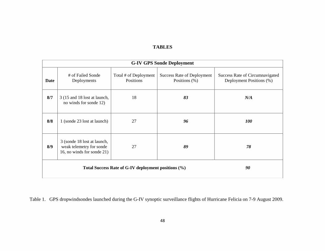
48

TABLES

Table 1. GPS dropwindsondes launched during the G-IV synoptic surveillance flights of Hurricane Felicia on 7-9 August 2009.

G-IV GPS Sonde Deployment

Date

# of Failed Sonde

Deployments

Total # of Deployment

Positions

Success Rate of Deployment

Positions (%)

Success Rate of Circumnavigated

Deployment Positions (%)

8/7

3 (15 and 18 lost at launch,

no winds for sonde 12)

18

83

N/A

8/8

1 (sonde 23 lost at launch)

27

96

100

8/9

3 (sonde 18 lost at launch,

weak telemetry for sonde

16, no winds for sonde 21)

27

89

78

Total Success Rate of G-IV deployment positions (%) 90

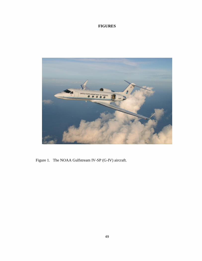
49

FIGURES

Figure 1. The NOAA Gulfstream IV-SP (G-IV) aircraft.

50

Figure 2. NOAA G-IV flight route in the Atlantic basin during TS Bonnie in July 2010.

Sonde deployments 14-26 represent a 3o circumnavigation around the center of the

circulation (Courtesy of NOAA HRD).

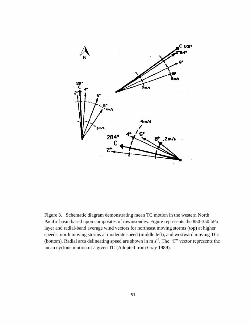
51

Figure 3. Schematic diagram demonstrating mean TC motion in the western North

Pacific basin based upon composites of rawinsondes. Figure represents the 850-350 hPa

layer and radial-band average wind vectors for northeast moving storms (top) at higher

speeds, north moving storms at moderate speed (middle left), and westward moving TCs

(bottom). Radial arcs delineating speed are shown in m s-1

. The “C” vector represents the

mean cyclone motion of a given TC (Adopted from Gray 1989).

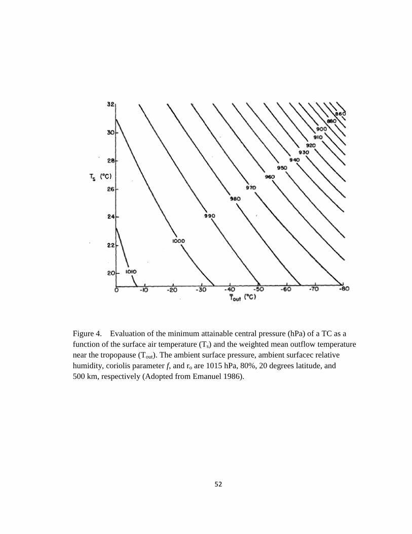
52

Figure 4. Evaluation of the minimum attainable central pressure (hPa) of a TC as a

function of the surface air temperature (Ts) and the weighted mean outflow temperature

near the tropopause (Tout). The ambient surface pressure, ambient surfacec relative

humidity, coriolis parameter f, and ro are 1015 hPa, 80%, 20 degrees latitude, and

500 km, respectively (Adopted from Emanuel 1986).

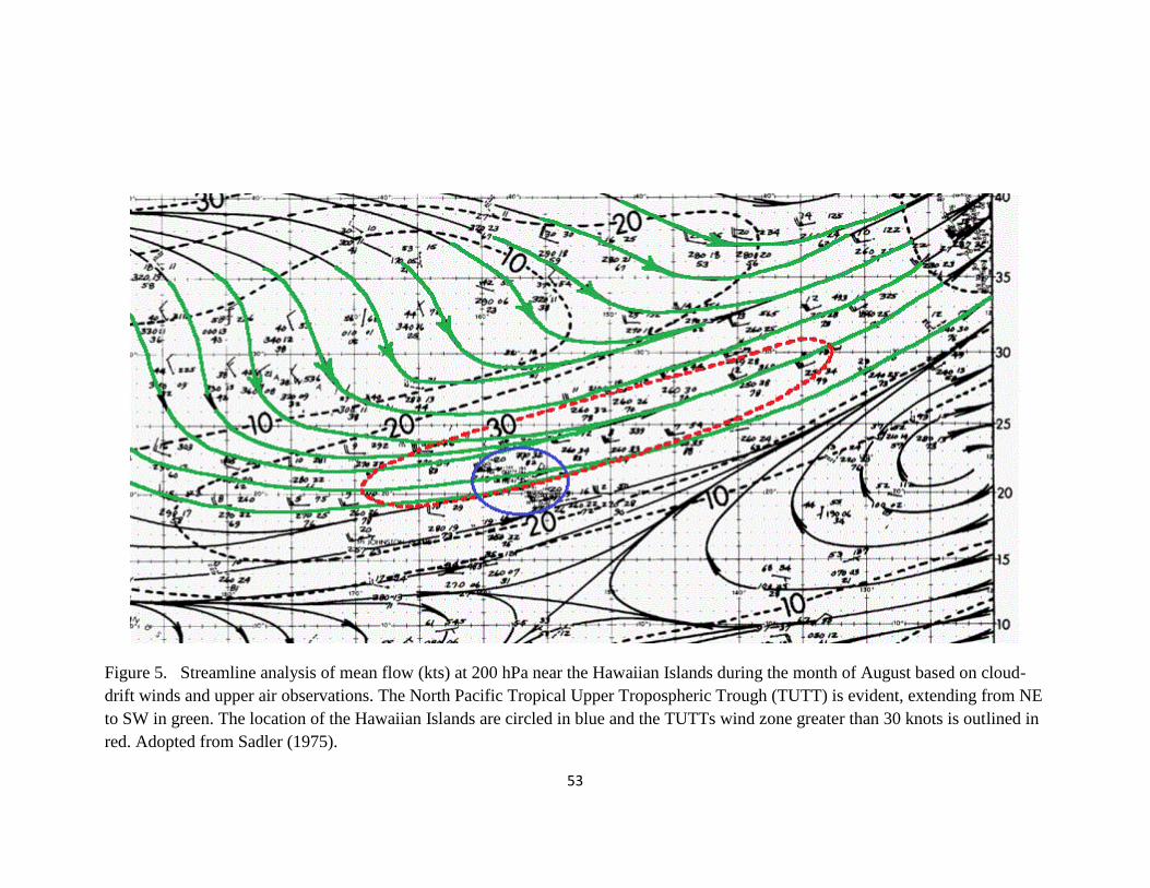
53

Figure 5. Streamline analysis of mean flow (kts) at 200 hPa near the Hawaiian Islands during the month of August based on cloud-

drift winds and upper air observations. The North Pacific Tropical Upper Tropospheric Trough (TUTT) is evident, extending from NE

to SW in green. The location of the Hawaiian Islands are circled in blue and the TUTTs wind zone greater than 30 knots is outlined in

red. Adopted from Sadler (1975).

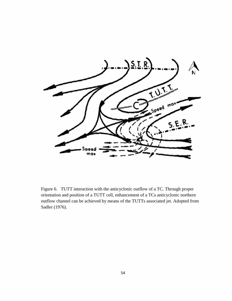
54

Figure 6. TUTT interaction with the anticyclonic outflow of a TC. Through proper

orientation and position of a TUTT cell, enhancement of a TCs anticyclonic northern

outflow channel can be achieved by means of the TUTTs associated jet. Adopted from

Sadler (1976).

55

Figure 7. Average August 850-200 hPa VWS values in m s-1

from 1966-2005. Adopted

from Dettmer (2011).

56

Figure 8. NOAA G-IV surveillance mission of Felicia on 7 August 2009 and chronological deployment distribution of GPS sondes.

The red markers denote unsuccessful sonde deployment locations. The green circle is Felicia’s low-level circulation center.

57

Figure 9. NOAA G-IV surveillance mission on 8 August 2009 and chronological deployment distribution of GPS sondes. The red

marker denotes an unsuccessful sonde deployment location. The green circle is Felicia’s low-level circulation center.

58

Figure 10. NOAA G-IV surveillance mission on 9 August 2009 and chronological deployment distribution of GPS sondes. The red

markers denote unsuccessful sonde deployment locations. The green circle is Felicia’s low- level circulation center.

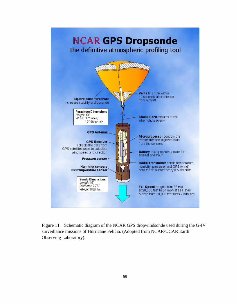
59

Figure 11. Schematic diagram of the NCAR GPS dropwindsonde used during the G-IV

surveillance missions of Hurricane Felicia. (Adopted from NCAR/UCAR Earth

Observing Laboratory).

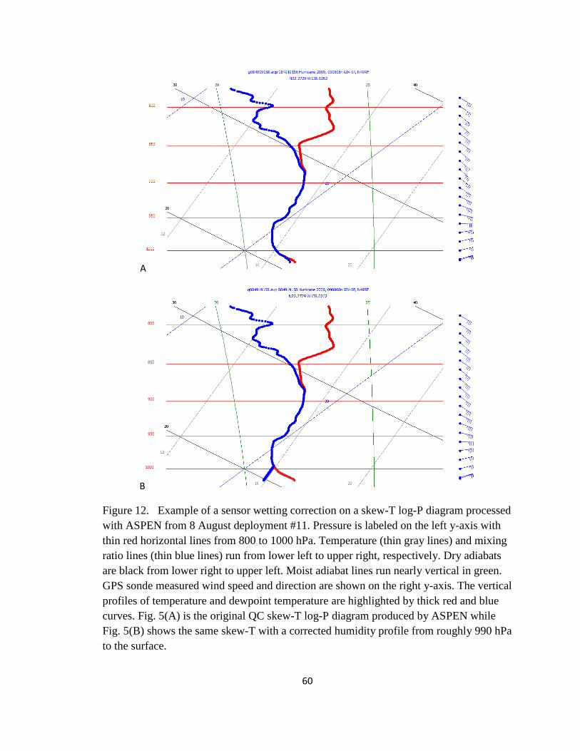
60

A

B

Figure 12. Example of a sensor wetting correction on a skew-T log-P diagram processed

with ASPEN from 8 August deployment #11. Pressure is labeled on the left y-axis with

thin red horizontal lines from 800 to 1000 hPa. Temperature (thin gray lines) and mixing

ratio lines (thin blue lines) run from lower left to upper right, respectively. Dry adiabats

are black from lower right to upper left. Moist adiabat lines run nearly vertical in green.

GPS sonde measured wind speed and direction are shown on the right y-axis. The vertical

profiles of temperature and dewpoint temperature are highlighted by thick red and blue

curves. Fig. 5(A) is the original QC skew-T log-P diagram produced by ASPEN while

Fig. 5(B) shows the same skew-T with a corrected humidity profile from roughly 990 hPa

to the surface.

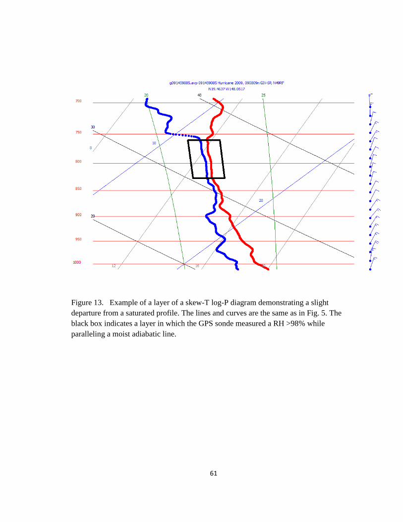
61

Figure 13. Example of a layer of a skew-T log-P diagram demonstrating a slight

departure from a saturated profile. The lines and curves are the same as in Fig. 5. The

black box indicates a layer in which the GPS sonde measured a RH >98% while

paralleling a moist adiabatic line.

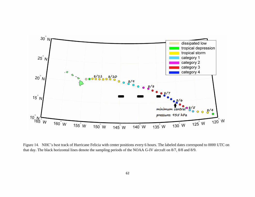
62

Figure 14. NHC’s best track of Hurricane Felicia with center positions every 6 hours. The labeled dates correspond to 0000 UTC on

that day. The black horizontal lines denote the sampling periods of the NOAA G-IV aircraft on 8/7, 8/8 and 8/9.

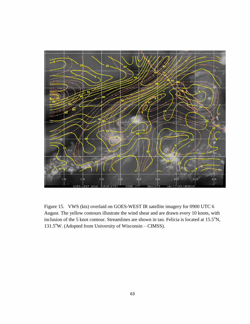
63

Figure 15. VWS (kts) overlaid on GOES-WEST IR satellite imagery for 0900 UTC 6

August. The yellow contours illustrate the wind shear and are drawn every 10 knots, with

inclusion of the 5 knot contour. Streamlines are shown in tan. Felicia is located at 15.5oN,

131.5oW. (Adopted from University of Wisconsin – CIMSS).

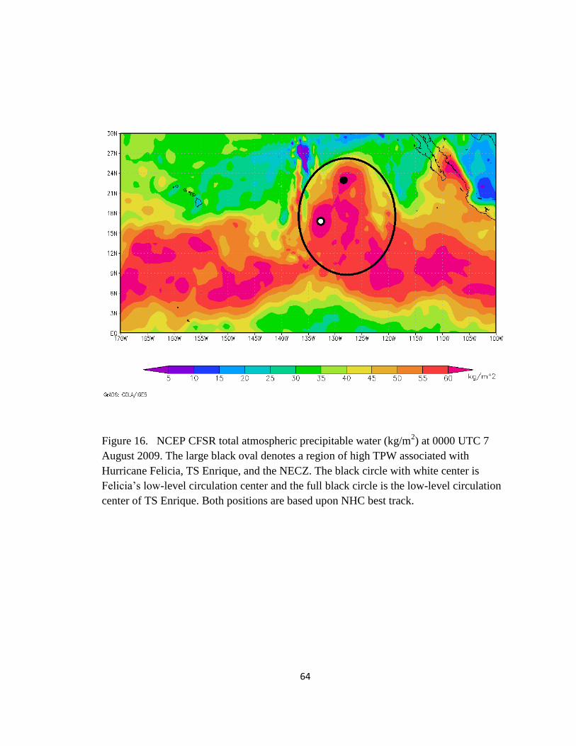
64

Figure 16. NCEP CFSR total atmospheric precipitable water (kg/m2) at 0000 UTC 7

August 2009. The large black oval denotes a region of high TPW associated with

Hurricane Felicia, TS Enrique, and the NECZ. The black circle with white center is

Felicia’s low-level circulation center and the full black circle is the low-level circulation

center of TS Enrique. Both positions are based upon NHC best track.

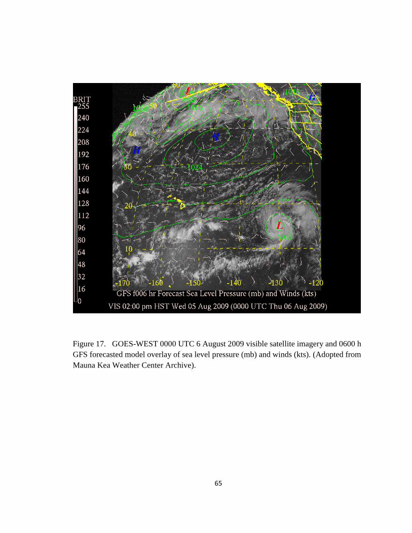
65

Figure 17. GOES-WEST 0000 UTC 6 August 2009 visible satellite imagery and 0600 h

GFS forecasted model overlay of sea level pressure (mb) and winds (kts). (Adopted from

Mauna Kea Weather Center Archive).

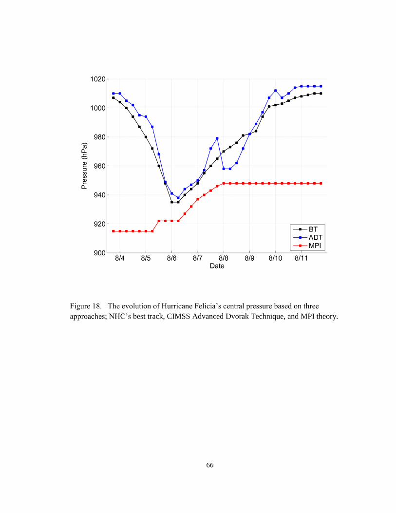
66

Figure 18. The evolution of Hurricane Felicia’s central pressure based on three

approaches; NHC’s best track, CIMSS Advanced Dvorak Technique, and MPI theory.

67

Figure 19. NOAA OIV2 weekly averaged satellite derived SSTs (oC) beginning 0000 UTC 5 August 2009 for the domain 180

oW to

120oW, 0

oN to 30

oN. Overlaid on this SST field is the complete track of Hurricane Felicia based upon best track. Black dots denote

0000 UTC of the labeled day. (Adapted from NOAA).

68

(a)

(b)

69

(c)

(d)

Figure 20. Color enhanced IR satellite imagery on (a) 1500 UTC 7 August (b) 1800 UTC 7

August (c) 2100 UTC 7 August and (d) 0000 UTC 8 August. Green color is <-50 oC, red is

<-70 oC.

70

Figure 21. Visible satellite imagery of Hurricane Felicia at 1800 UTC 7 August. Grid is every

2 degrees latitude or longitude.

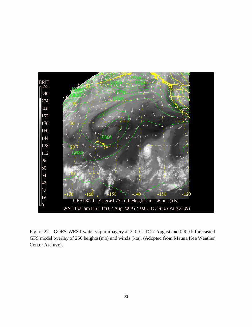
71

Figure 22. GOES-WEST water vapor imagery at 2100 UTC 7 August and 0900 h forecasted

GFS model overlay of 250 heights (mb) and winds (kts). (Adopted from Mauna Kea Weather

Center Archive).

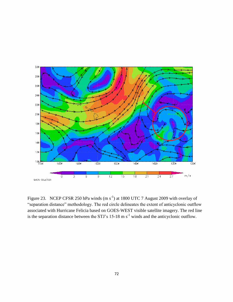
72

Figure 23. NCEP CFSR 250 hPa winds (m s-1

) at 1800 UTC 7 August 2009 with overlay of

“separation distance” methodology. The red circle delineates the extent of anticyclonic outflow

associated with Hurricane Felicia based on GOES-WEST visible satellite imagery. The red line

is the separation distance between the STJ’s 15-18 m s-1

winds and the anticyclonic outflow.

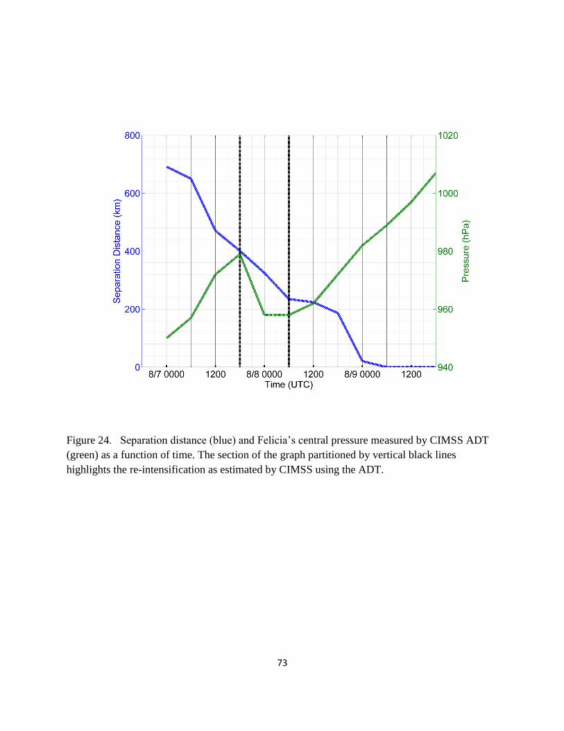
73

Figure 24. Separation distance (blue) and Felicia’s central pressure measured by CIMSS ADT

(green) as a function of time. The section of the graph partitioned by vertical black lines

highlights the re-intensification as estimated by CIMSS using the ADT.

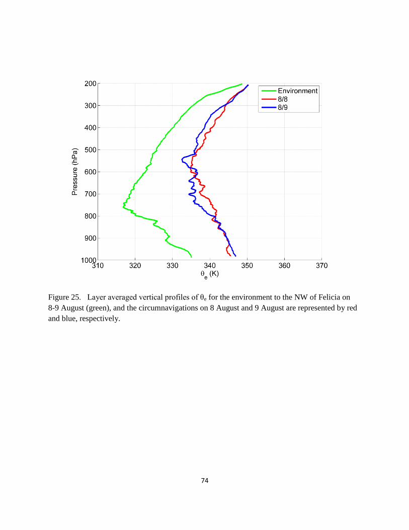
74

Figure 25. Layer averaged vertical profiles of θe for the environment to the NW of Felicia on

8-9 August (green), and the circumnavigations on 8 August and 9 August are represented by red

and blue, respectively.

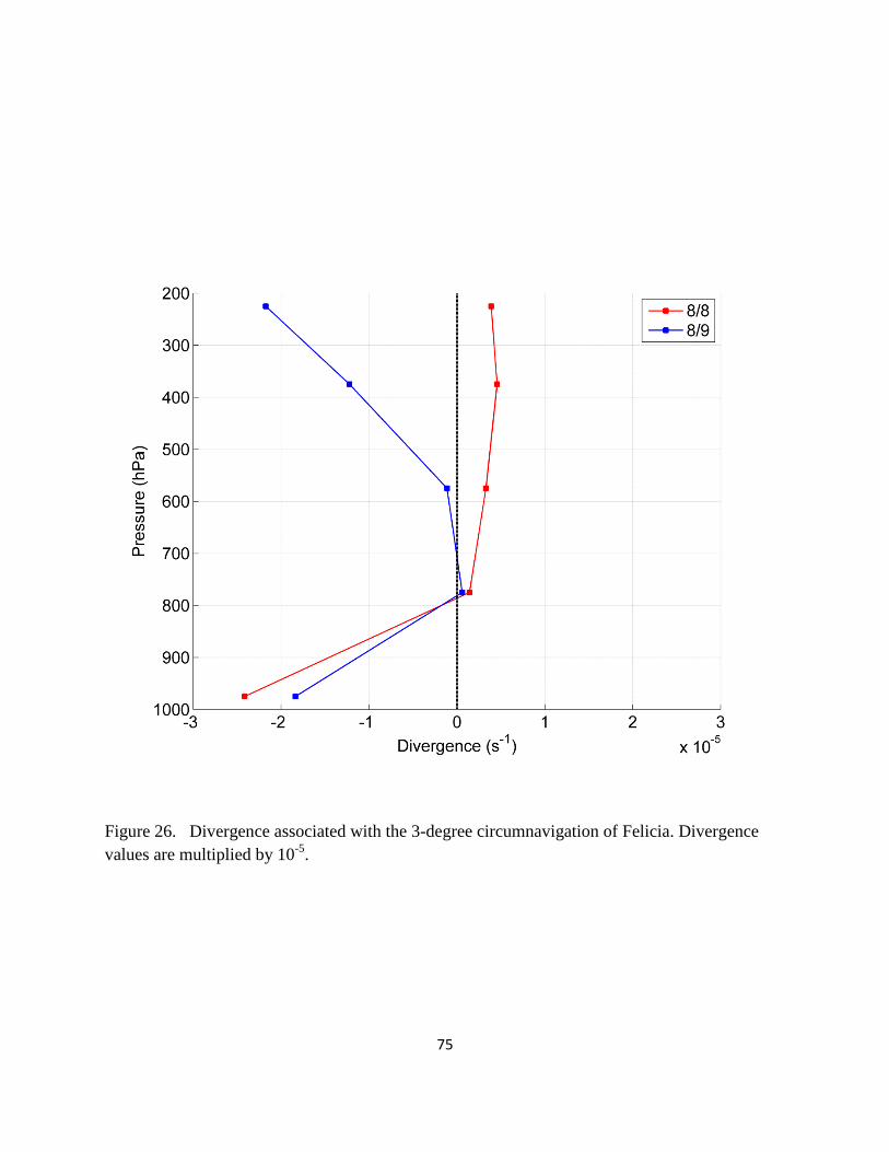
75

Figure 26. Divergence associated with the 3-degree circumnavigation of Felicia. Divergence

values are multiplied by 10-5

.

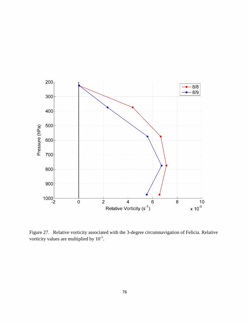
76

Figure 27. Relative vorticity associated with the 3-degree circumnavigation of Felicia. Relative

vorticity values are multiplied by 10-5

.

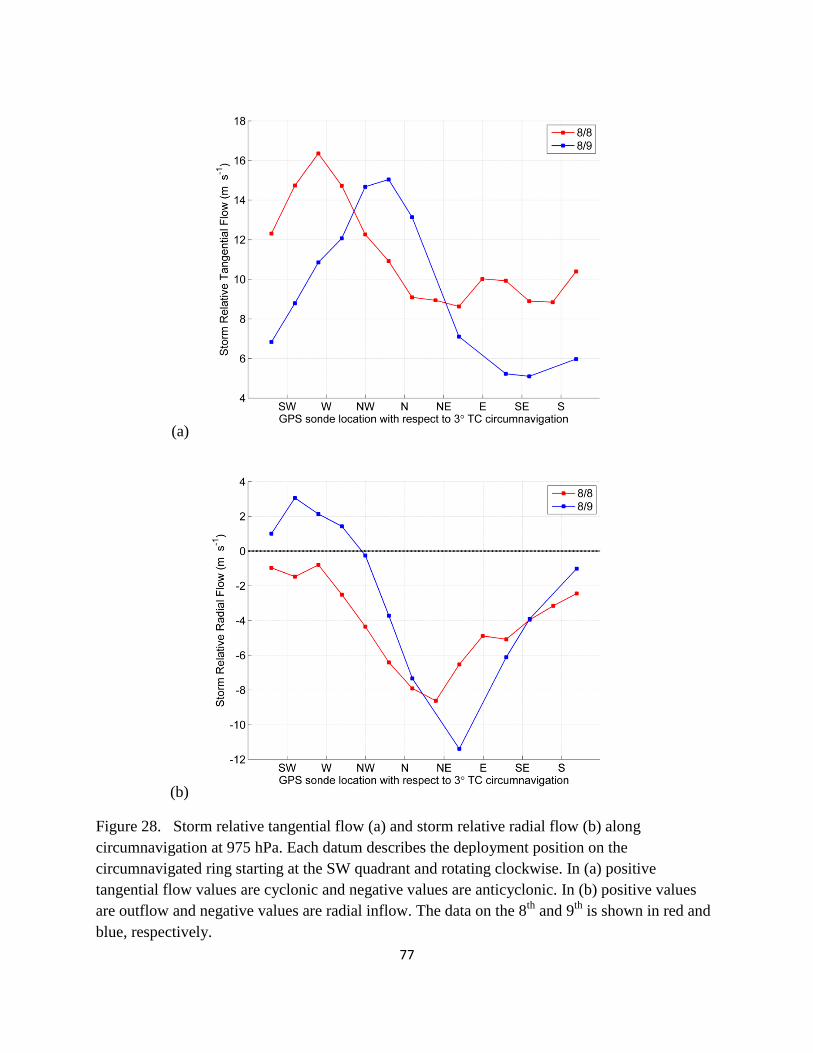
77

(a)

(b)

Figure 28. Storm relative tangential flow (a) and storm relative radial flow (b) along

circumnavigation at 975 hPa. Each datum describes the deployment position on the

circumnavigated ring starting at the SW quadrant and rotating clockwise. In (a) positive

tangential flow values are cyclonic and negative values are anticyclonic. In (b) positive values

are outflow and negative values are radial inflow. The data on the 8th

and 9th

is shown in red and

blue, respectively.

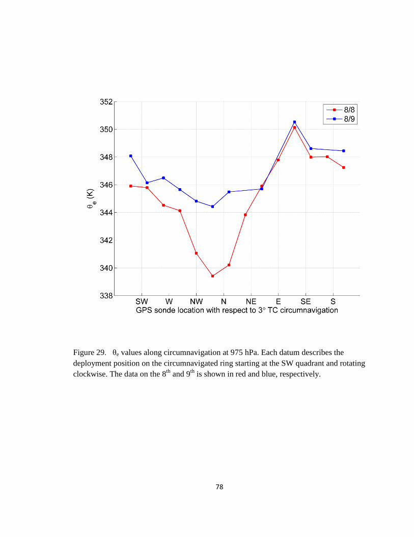
78

Figure 29. θe values along circumnavigation at 975 hPa. Each datum describes the

deployment position on the circumnavigated ring starting at the SW quadrant and rotating

clockwise. The data on the 8th

and 9th

is shown in red and blue, respectively.

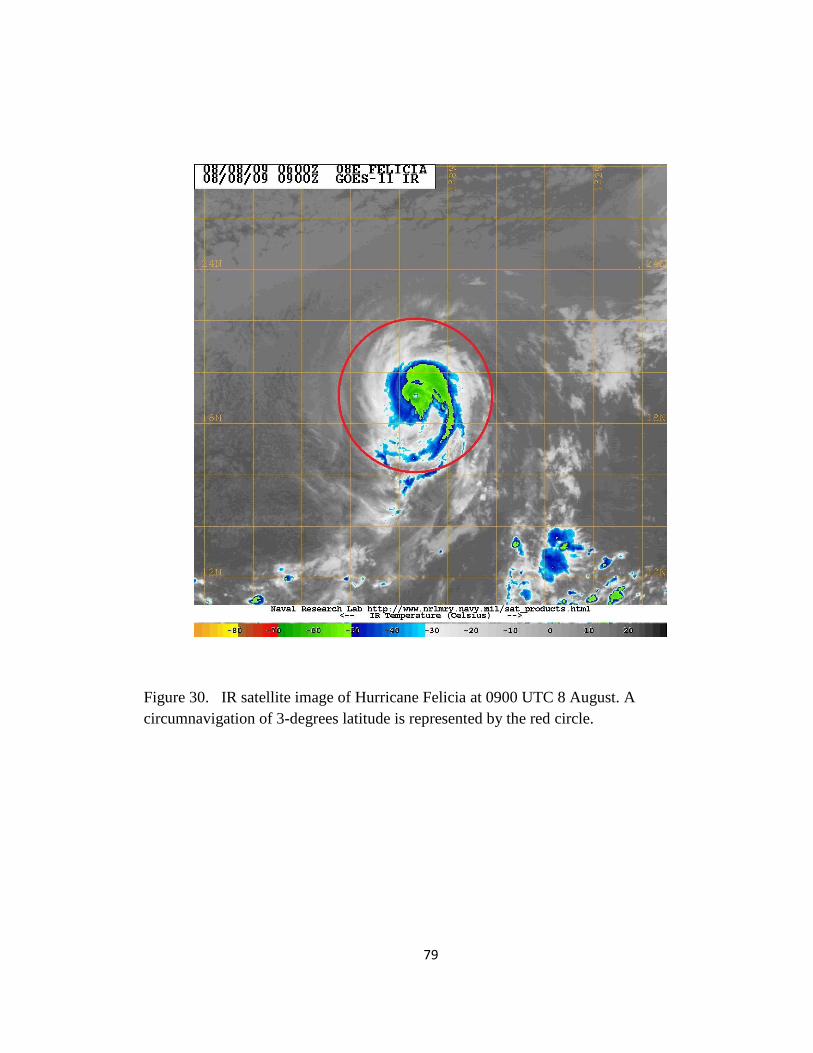
79

Figure 30. IR satellite image of Hurricane Felicia at 0900 UTC 8 August. A

circumnavigation of 3-degrees latitude is represented by the red circle.

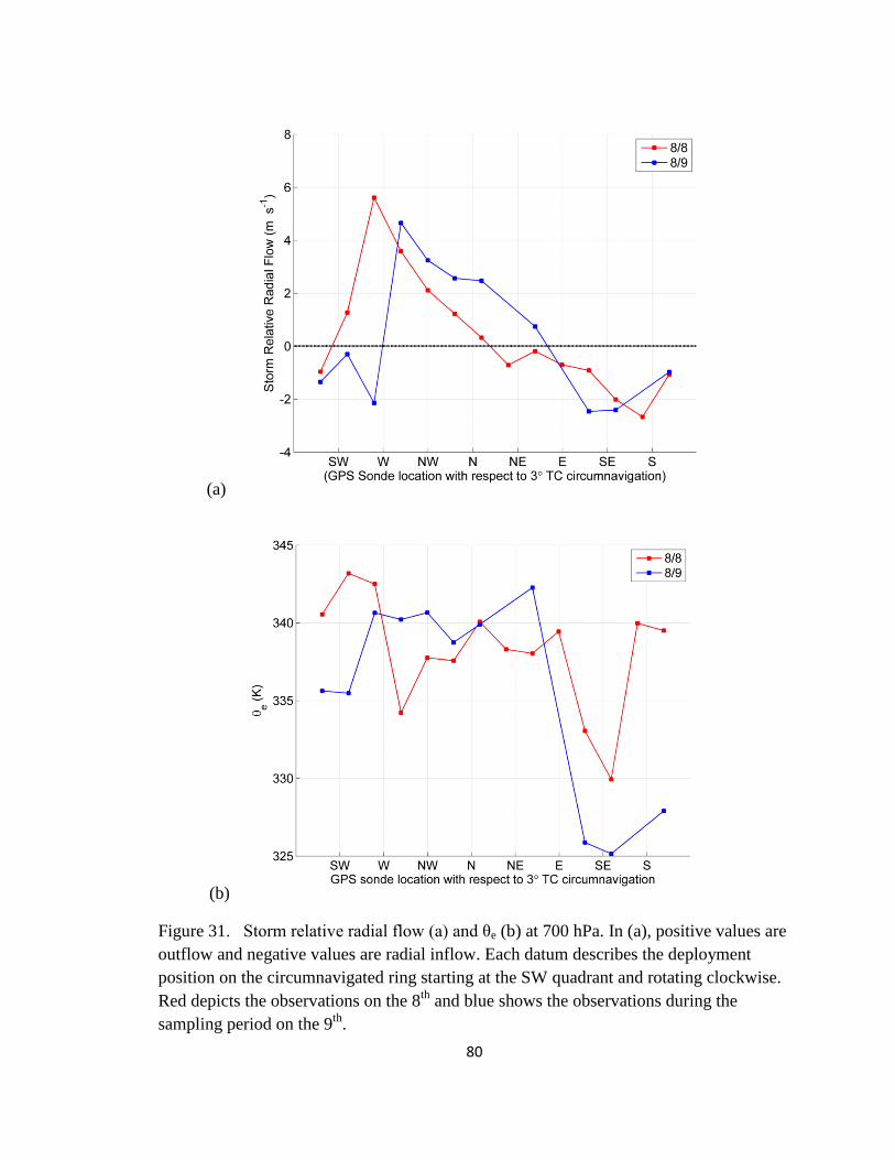
80

(a)

(b)

Figure 31. Storm relative radial flow (a) and θe (b) at 700 hPa. In (a), positive values are

outflow and negative values are radial inflow. Each datum describes the deployment

position on the circumnavigated ring starting at the SW quadrant and rotating clockwise.

Red depicts the observations on the 8th

and blue shows the observations during the

sampling period on the 9th

.

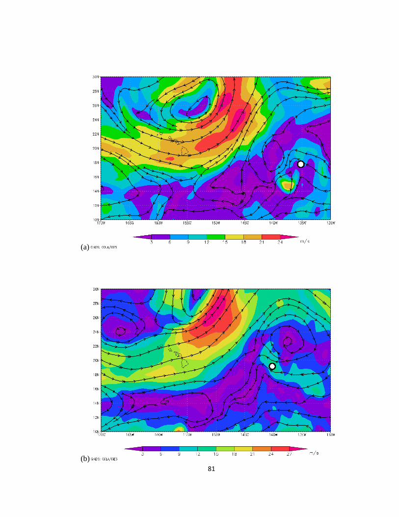
81

(a)

(b)

82

(c)

Figure 32. NCEP CFSR 250 hPa winds (m/s) for (a) 1200 UTC 7 August, (b) 1200 UTC

8 August, and (c) 1200 UTC 9 August. The low-level circulation center of Felicia in each

panel is represented by the white and black circle.

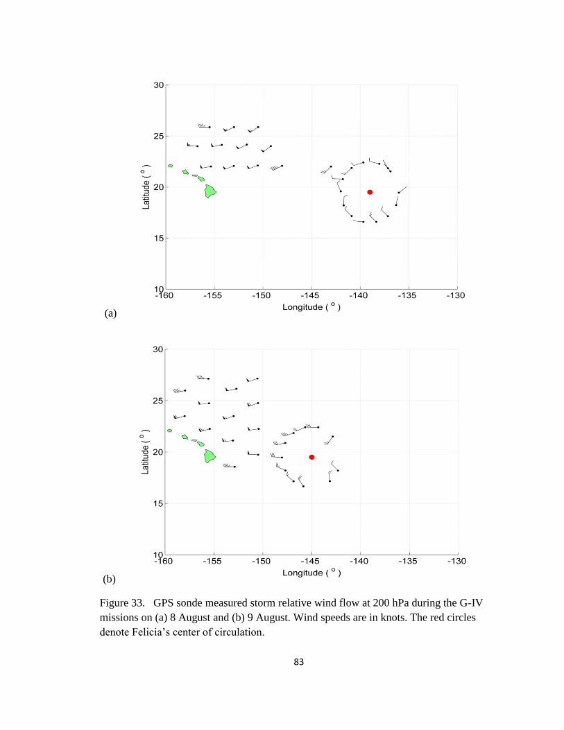
83

(a)

(b)

Figure 33. GPS sonde measured storm relative wind flow at 200 hPa during the G-IV

missions on (a) 8 August and (b) 9 August. Wind speeds are in knots. The red circles

denote Felicia’s center of circulation.

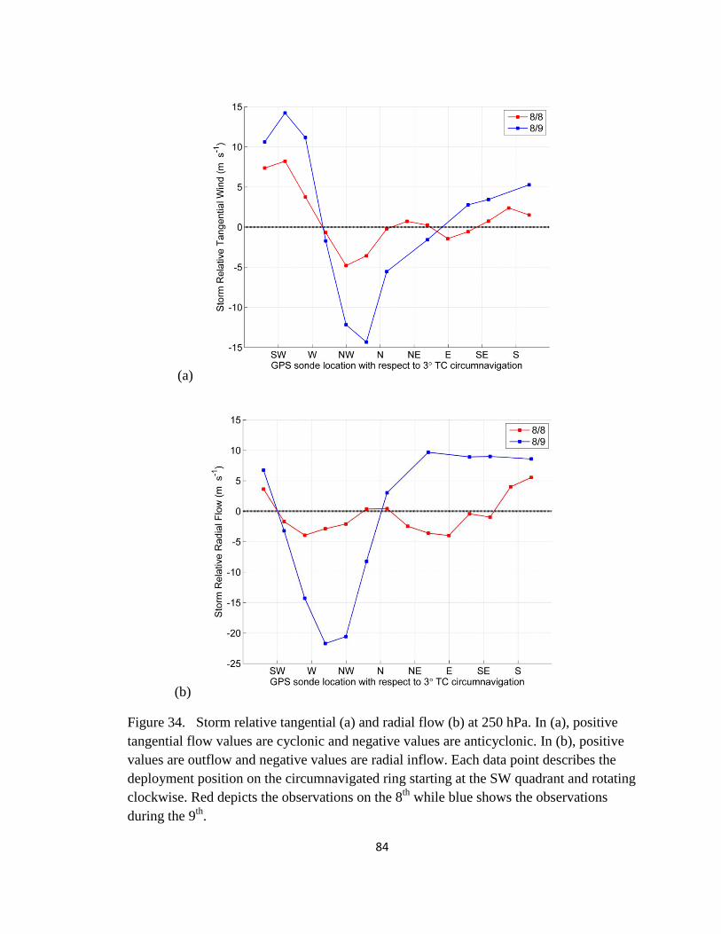
84

(a)

(b)

Figure 34. Storm relative tangential (a) and radial flow (b) at 250 hPa. In (a), positive

tangential flow values are cyclonic and negative values are anticyclonic. In (b), positive

values are outflow and negative values are radial inflow. Each data point describes the

deployment position on the circumnavigated ring starting at the SW quadrant and rotating

clockwise. Red depicts the observations on the 8th

while blue shows the observations

during the 9th

.

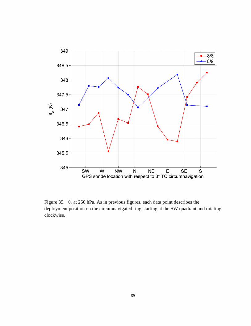
85

Figure 35. θe at 250 hPa. As in previous figures, each data point describes the

deployment position on the circumnavigated ring starting at the SW quadrant and rotating

clockwise.

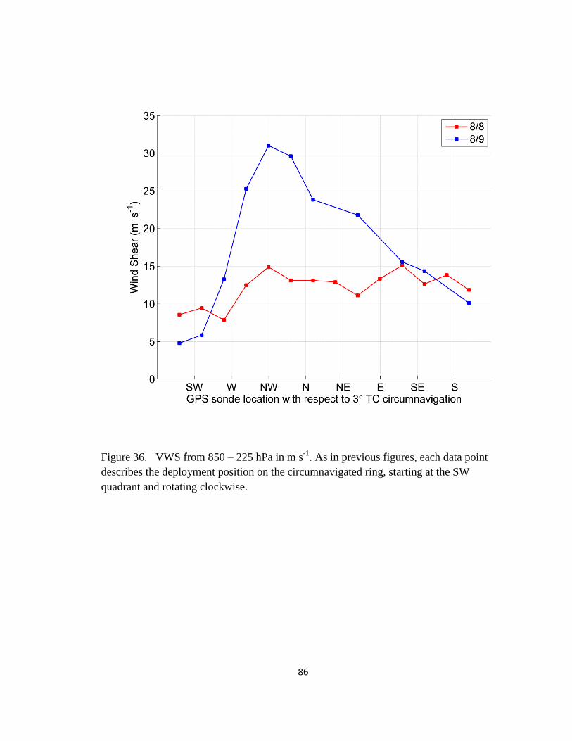
86

Figure 36. VWS from 850 – 225 hPa in m s-1

. As in previous figures, each data point

describes the deployment position on the circumnavigated ring, starting at the SW

quadrant and rotating clockwise.

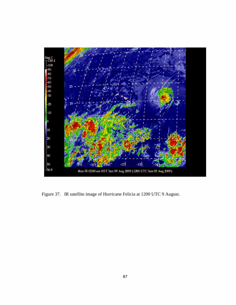
87

Figure 37. IR satellite image of Hurricane Felicia at 1200 UTC 9 August.

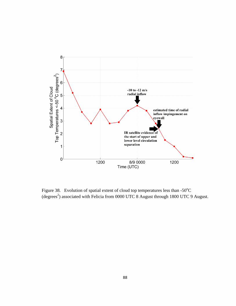
88

Figure 38. Evolution of spatial extent of cloud top temperatures less than -50oC

(degrees2) associated with Felicia from 0000 UTC 8 August through 1800 UTC 9 August.

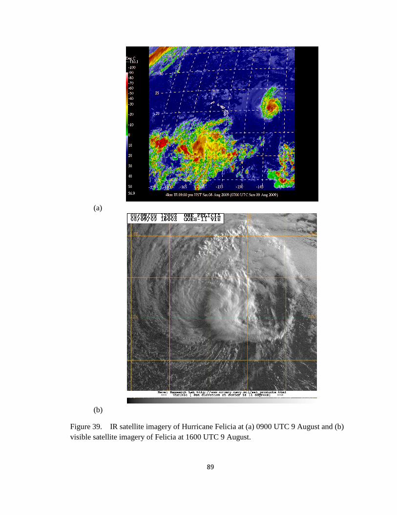
89

(a)

(b)

Figure 39. IR satellite imagery of Hurricane Felicia at (a) 0900 UTC 9 August and (b)

visible satellite imagery of Felicia at 1600 UTC 9 August.

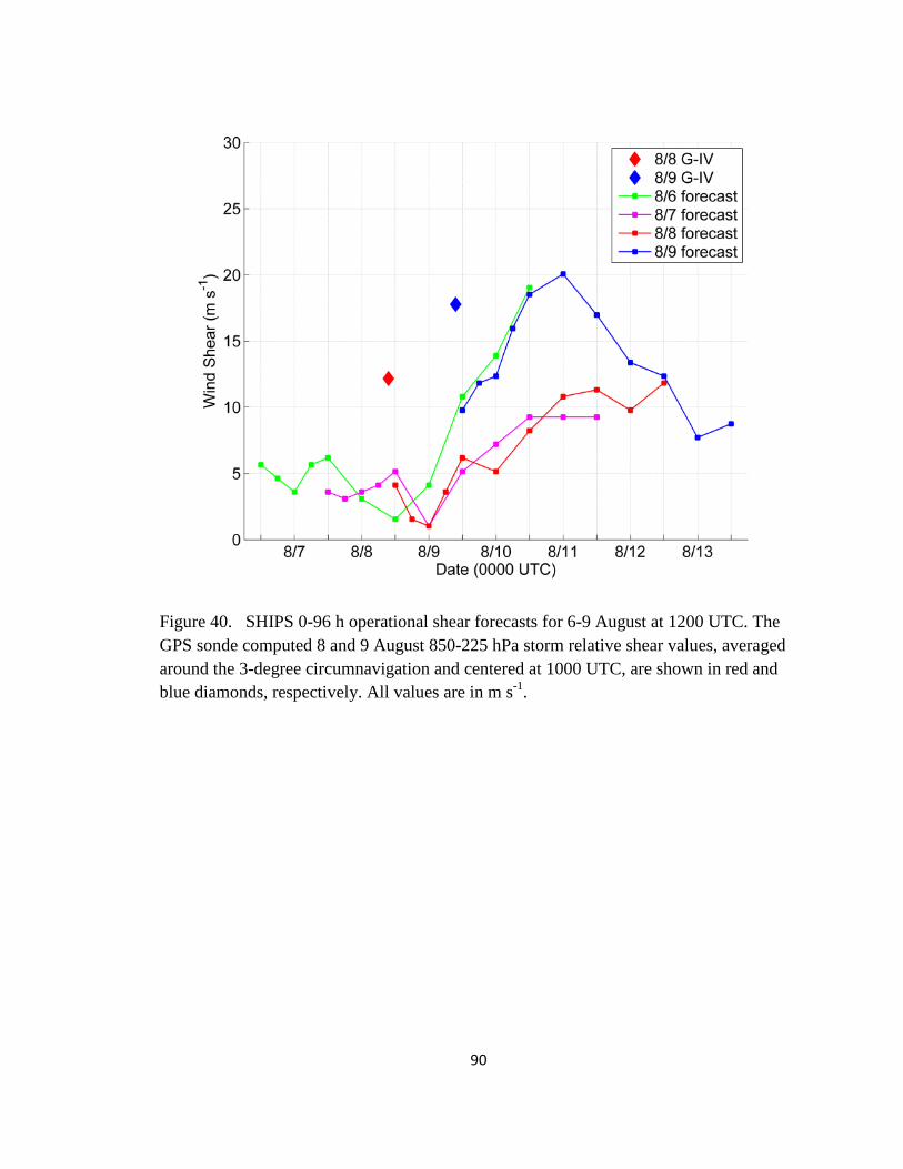
90

Figure 40. SHIPS 0-96 h operational shear forecasts for 6-9 August at 1200 UTC. The

GPS sonde computed 8 and 9 August 850-225 hPa storm relative shear values, averaged

around the 3-degree circumnavigation and centered at 1000 UTC, are shown in red and

blue diamonds, respectively. All values are in m s-1

.

91

REFERENCES

Avila, L. A., 1998: Forecasting tropical cyclone intensity changes: An operational

challenge. Preprints, Symp. on Tropical Cyclone Intensity Change, Phoenix, AZ,

Amer. Meteor. Soc., 1–3.

Barnes, G. M., E. J. Zipser, D. Jorgensen, and F. Marks, 1983: Mesoscale and convective

structure of a hurricane rainband. J. Atmos. Sci., 40, 2125–2137.

________, 2008: Atypical thermodynamic profiles in hurricanes. Mon. Wea. Rev., 136,

631–643.

Black, M. L., J. F. Gamache, F. D. Marks Jr., C. E. Samsury, and H. E. Willoughby,

2002: Eastern Pacific Hurricanes Jimena of 1991 and Olivia of 1994: The effect

of vertical shear on structure and intensity. Mon. Wea. Rev., 130, 2291–2312.

Black, P. G., and R. A. Anthes, 1971: On the asymmetric structure of the tropical

cyclone outflow layer. J. Atmos. Sci., 28, 1348–1366.

Bogner, P. B., G. M. Barnes, and J. L. Franklin, 2000: Conditional instability and shear

for six hurricanes over the Atlantic Ocean. Wea. Forecasting, 15, 192–207.

Bolton, D., 1980: The computation of equivalent potential temperature. Mon. Wea.

Rev., 108, 1046–1053.

Bosart, L. F., W. E. Bracken, J. Molinari, C. S. Velden, and P. G. Black, 2000:

Environmental influences on the rapid intensification of Hurricane Opal (1995)

over the Gulf of Mexico. Mon. Wea. Rev., 128, 322–352.

Braun, S. A., 2010: Reevaluating the role of the Saharan air layer in Atlantic tropical

cyclogenesis and evolution. Mon. Wea. Rev., 138, 2007–2037.

________, J. A. Sippel, and D. S. Nolan, 2012: The impact of dry midlevel air on

hurricane intensity in idealized simulations with no mean flow. J. Atmos. Sci., 69,

236–257.

Burpee, R. W., S. D. Aberson, J. L. Franklin, S. J. Lord, and R. E. Tuleya, 1996: The

impact of Omega Dropwindsondes on operational hurricane track forecast

Models. Bull. Amer. Meteor. Soc., 77, 925–933.

Chen, G., and L. F. Chou, 1994: An investigation of cold vortices in the upper

troposphere over the western North Pacific during the warm season. Mon. Wea.

Rev., 122, 1436-1448.

92

Cione, J. J., and E. W. Uhlhorn, 2003: Sea surface temperature variability in

Hurricanes: Implications with respect to intensity change. Mon. Wea. Rev., 131,

1783–1796.

Cooperative Institute for Meteorological Satellite Studies and University of Wisconsin-

Madison. (2012). CIMSS Tropical Cyclones Data Archive. Retrieved from

http://tropic.ssec.wisc.edu/archive/

Dare, R. A., J. L. McBride, 2011: The Threshold sea surface temperature condition

for tropical cyclogenesis. J. Climate, 24, 4570–4576.

DeMaria, M., J-J. Baik, and J. Kaplan, 1993: Upper-level eddy angular momentum fluxes

and tropical cyclone intensity change. J. Atmos. Sci., 50, 1133–1147.

________, and J. Kaplan, 1994: A statistical hurricane intensity prediction scheme

(SHIPS) for the Atlantic basin. Wea. Forecasting, 9, 209–220.

________, 1996: The effect of vertical shear on tropical cyclone intensity change. J.

Atmos. Sci., 53, 2076-2088.

Dengler, K., 1997: A numerical study of the effects of land proximity and changes in sea

surface temperature on hurricane tracks. Quart. J. Roy. Meteor. Soc., 123, 1307–

1321.

Dolling, K. P., 2012: The Evolution of Hurricane Humberto (2001). Ph.D. dissertation,

University of Hawaii at Manoa, Honolulu, HI, 000 pp.

________, and G. M. Barnes, 2012: The creation of a high equivalent potential

temperature reservoir in Tropical Storm Humberto (2001) and its possible role in

storm deepening. Mon. Wea. Rev., 140, 492–505.

________, and G. M. Barnes, 2014: The Evolution of Hurricane Humberto (2001). J.

Atmos. Sci., 71, 1276–1291.

Dunion, J. P., and C. S. Velden, 2004: The impact of the Saharan air layer on Atlantic

tropical cyclone activity. Bull. Amer. Meteor. Soc., 85, 353–365.

Emanuel, K. A., 1986: An air-sea interaction theory for tropical cyclones. Part I:

Steady state maintenance. J. Atmos. Sci., 43, 585–605.

Frank, F. M., 1977: The structure and energetics of the tropical cyclone I. Storm

structure. Mon. Wea. Rev., 105, 1119–1135.

93

Frank, W. M., and E. A. Ritchie, 2001: Effects of vertical wind shear on the

intensity and structure of numerically simulated hurricanes. Mon. Wea. Rev., 129,

2249–2269.

Franklin, J. L., 1990: Dropwindsonde observations of the environmental flow of

hurricane Josephine (1984): Relationships to vortex motion. Mon Wea. Rev., 118,

2732-2744.

Gallina, G., and C. Velden, 2002: Environmental vertical wind shear and tropical cyclone

intensity change utilizing enhanced satellite derived wind information. Preprints,

25th

Conf. on Hurricanes and Tropical Meteorology, San Diego, CA, Amer.

Meteor. Soc., 172-173.

Gray, W. M., 1968: Global view of the origin of tropical disturbances and storms.

Mon. Wea. Rev., 96, 669–700.

________, 1989: Summary of ONR sponsored tropical cyclone motion research and

future plans. Appendix D of Technical Report NPS 63-89-002, Naval

Postgraduate School (R.L. Elsberry, Ed.), Monterey, CA 93943, 68-79.

Hock, T. F., and J. L. Franklin, 1999: The NCAR GPS Dropwindsonde. Bull. Amer.

Meteor. Soc., 80, 407–420.

Holland, G. J., and R. T. Merrill, 1984: On the dynamics of tropical cyclone structural

changes. Quart. J. Roy. Meteor. Soc., 110, 723-745.

Kimberlain, T. B., R. D. Knabb, and D. Wroe, 2010: Tropical Cyclone Report: Hurricane

Felicia (EP082009). Retrieved from

http://www.nhc.noaa.gov/pdf/TCR-EP082009_Felicia.pdf

Malkus, J. S., and H. Riehl, 1960: On the dynamics and energy transformation in steady-

state hurricanes. Tellus, 12, 1-20.

Marin, J., D. Raymond, and G. Raga, 2009: Intensification of tropical cyclones in the

GFS model. Atmos. Chem. Phys., 9, 1407-1417.

Martin, C., 2007: ASPEN User Manual. NCAR, 61pp. {Available online at

http://www.eol.ucar.edu/isf/facilities/software/aspen/ASPEN%20Manual.pdf}

McBride, J., and R. Zehr, 1981: Observational analysis of tropical cyclone formation.

Part II: Comparison of non-developing versus developing systems. J. Atmos. Sci.,

38, 1132-1151.

94

Miller, B. I., 1958: On the maximum intensity of hurricanes. J. Meteor., 15, 184–195.

________, 1964: A study of the filling of Hurricane Donna (1960) over land. Mon. Wea.

Rev., 9, 389-406.

NOAA_OI_SST_V2 data provided by the NOAA/OAR/ESRL PSD, Boulder, Colorado,

USA, http://www.esrl.noaa.gov/psd/

Nolan, D. S., 2007: What is the trigger for tropical cyclogenesis? Aust. Meteor. Mag., 56,

241–266.

Palmén, E. H., 1948: On the formation and structure of tropical cyclones. Geophysics, 3,

26–38.

Patla, J. E., D. Stevens, and G. M. Barnes, 2009: A conceptual model for the influence

of TUTT cells on tropical cyclone motion in the Northwest Pacific Ocean. Wea.

Forecasting, 24, 1215–1235.

Powell, M. D., 1990: Boundary layer structure and dynamics in outer hurricane

rainbands. Part II: Downdraft modification and mixed layer recovery. Mon. Wea.

Rev., 118, 918–938.

________, S. H. Houston, L. R. Amat, and N. Morisseau-Leroy, 1998: The HRD

real-time hurricane wind analysis system. J. Wind Engineer. and Indust. Aerodyn.

77&78, 53-64

Reynolds, R. W., 1988: A real-time global sea surface temperature analysis. J. Climate,

1, 75-86.

________, D. C. Marsico, 1993: An improved real-time global sea surface temperature

analysis. J. Climate, 6, 114-119.

Riemer, M., M. Montgomery, and M. Nicholls, 2010: A new paradigm for intensity

modification of tropical cyclones: Thermodynamic impact of vertical wind shear

on the inflow layer. Atmos. Chem. Phys., 10, 3163-3188.

Rogers, R., and Coauthors, 2006: The intensity forecasting experiment: A NOAA

multiyear field program for improving tropical cyclone intensity forecasts. Bull.

Amer. Meteor. Soc., 87, 1523–1537.

95

Sadler, J. C., 1967: The tropical upper tropospheric trough as a secondary source of

typhoons and primary source of trade wind disturbances. Hawaii Institute of

Geophysics, Rep. 67-12, 103 pp.

________, 1975: The upper tropospheric circulation over the global tropics. Dept. of

Meteorology Rep. UHMET-75-05, University of Hawaii, Honolulu, HI, 16 pp.

________, 1976: A role of the tropical upper tropospheric trough in early season

typhoon development. Mon. Wea. Rev., 104, 1266–1278.

________, 1978: Mid-season typhoon development and intensity changes and the

tropical upper tropospheric trough. Mon. Wea. Rev., 106, 1137–1152.

Saha, S., et al. 2010. NCEP Climate Forecast System Reanalysis (CFSR) 6-hourly

Products, January 1979 to December 2010. Research data archive at the National

Center for Atmospheric Research, Computational and Information Systems

Laboratory. http://dx.doi.org/10.5065/D69K487J. Accessed 23 Sept 2014.

Simpson R., and H. Riehl, 1958: Mid-tropospheric ventilation as a constraint on

hurricane development and maintenance. Preprints, Tech. Conf. on Hurricanes,

Miami Beach, FL, Amer. Meteor. Soc., D4-1-D4-10.

Sippel, J. A., S. A. Braun, F. Zhang, and Y. Weng, 2013: Ensemble Kalman filter

assimilation of simulated HIWRAP Doppler velocity data in a hurricane. Mon.

Wea. Rev., 141, 2683–2704.

Shieh, O. H., M. Fiorino, M. E. Kucas, and B. Wang, 2013: Extreme rapid

intensification of Typhoon Vicente (2012) in the South China Sea. Wea.

Forecasting, 28, 1578–1587.

Shu, S. J., and L. Wu, 2009: Analysis of the influence of the Saharan air layer on tropical

cyclone intensity using AIRS/Aqua data. Geophys. Res. Lett., 36, L09809,

doi:10.1029/2009GL037634.

Tang, B., and K. Emanuel, 2012: A ventilation index for tropical cyclones. Bull. Amer.

Meteor. Soc., 93, 1901–1912.

Velden C. S., and J. Sears, 2014: Computing deep-tropospheric vertical wind shear

analyses for tropical cyclone applications: Does the methodology matter?. Wea.

Forecasting, 29, 1169–1180.

96

Wang, J., 2005: Evaluation of the dropsonde humidity sensor using data from DYCOMS-

II and IHOP_2002. J. Atmos. Oceanic. Technol., 22, 247-257.

Wu, L., 2007: Impact of Saharan air layer on hurricane peak intensity. Geophys. Res.

Lett., 34, L09802, doi:10.1029/2007GL029564.

Zehr, R., 1992: Tropical cyclogenesis in the western north Pacific. NOAA Tech. Rep.

NESDIS 61, 181 pp.

Zhang, C., 1993: Large-scale variability of atmospheric deep convection in relation to

sea surface temperature in the tropics. J. Climate, 6, 1898–1913.