Naval Research LaboratoryStennis Space Center, MS 39529-5004

NRL/MR/7320--10-9242

The Coastal Dynamics of HeterogeneousSedimentary Environments: NumericalModeling of Nearshore Hydrodynamicsand Sediment Transport

May 10, 2010

Approved for public release; distribution is unlimited.

TimoThy R. Keen

Ocean Dynamics and Prediction Branch Oceanography Division

K. Todd holland

Seafloor Sciences Branch Marine Geosciences Division

i

REPORT DOCUMENTATION PAGE Form ApprovedOMB No. 0704-0188

3. DATES COVERED (From - To)

Standard Form 298 (Rev. 8-98)Prescribed by ANSI Std. Z39.18

Public reporting burden for this collection of information is estimated to average 1 hour per response, including the time for reviewing instructions, searching existing data sources, gathering and maintaining the data needed, and completing and reviewing this collection of information. Send comments regarding this burden estimate or any other aspect of this collection of information, including suggestions for reducing this burden to Department of Defense, Washington Headquarters Services, Directorate for Information Operations and Reports (0704-0188), 1215 Jefferson Davis Highway, Suite 1204, Arlington, VA 22202-4302. Respondents should be aware that notwithstanding any other provision of law, no person shall be subject to any penalty for failing to comply with a collection of information if it does not display a currently valid OMB control number. PLEASE DO NOT RETURN YOUR FORM TO THE ABOVE ADDRESS.

5a. CONTRACT NUMBER

5b. GRANT NUMBER

5c. PROGRAM ELEMENT NUMBER

5d. PROJECT NUMBER

5e. TASK NUMBER

5f. WORK UNIT NUMBER

2. REPORT TYPE1. REPORT DATE (DD-MM-YYYY)

4. TITLE AND SUBTITLE

6. AUTHOR(S)

8. PERFORMING ORGANIZATION REPORT NUMBER

7. PERFORMING ORGANIZATION NAME(S) AND ADDRESS(ES)

10. SPONSOR / MONITOR’S ACRONYM(S)9. SPONSORING / MONITORING AGENCY NAME(S) AND ADDRESS(ES)

11. SPONSOR / MONITOR’S REPORT NUMBER(S)

12. DISTRIBUTION / AVAILABILITY STATEMENT

13. SUPPLEMENTARY NOTES

14. ABSTRACT

15. SUBJECT TERMS

16. SECURITY CLASSIFICATION OF:

a. REPORT

19a. NAME OF RESPONSIBLE PERSON

19b. TELEPHONE NUMBER (include areacode)

b. ABSTRACT c. THIS PAGE

18. NUMBEROF PAGES

17. LIMITATIONOF ABSTRACT

The Coastal Dynamics of Heterogeneous Sedimentary Environments:Numerical Modeling of Nearshore Hydrodynamics and SedimentTransport

Timothy R. Keen and K. Todd Holland

Naval Research LaboratoryOceanography DivisionStennis Space Center, MS 39529-5004

NRL/MR/7320--10-9242

Approved for public release; distribution is unlimited.

Unclassified Unclassified UnclassifiedSAR 145

Timothy Keen

(288) 688-4950

This report discusses details of the numerical models used to simulate wave, tide, and wind-driven hydrodynamics and sedimentation in water depths less than 10 m. These simulations have used the Princeton Ocean Model (POM), the Navy Coastal Ocean Model (NCOM), the SWAN wave model, and the Littoral Sedimentation and Optics Model (LSOM). The problems include: (1) nearshore erosion and mass conservation on the shoreface; (2) coastal erosion during a hurricane; (3) sand resuspension and optical characteristics on the shoreface; and (4) barrier island erosion during cold fronts. These results demonstrate several important conclusions: (a) the nearshore is an open system with respect to sediment transport; (b) nearshore hydrodynamics is not always dominated by waves but also relies on winds and tides; (c) very weak processes can have unforeseen impacts over long periods.

10-05-2010 Memorandum Report

Office of Naval ResearchOne Liberty Center875 North Randolph StreetArlington, VA 22203-1995

73-4261-00-5

ONR

SedimentationNearshore

0601153N

Numerical models

iii

Table of Contents 

1  Introduction ........................................................................................................................... 1 

1.1  Motivation .................................................................................................................. 1 

1.2  Background .................................................................................................................... 2 

1.3  Definitions ...................................................................................................................... 5 

2  Approach ............................................................................................................................... 8 

2.1  Observations and Modeled Oceanographic Databases .................................................. 9 

2.2  Numerical Models ........................................................................................................ 10 

2.2.1  Navy Coastal Ocean Model .................................................................................. 10 

2.2.2  Princeton Ocean Model......................................................................................... 11 

2.2.3  Shoreface Circulation Model (SHORECIRC) ...................................................... 11 

2.2.4  Simulating Waves Nearshore (SWAN) ................................................................ 12 

2.2.5  Littoral Sedimentation and Optics Model (LSOM) .............................................. 12 

2.3  Simulation .................................................................................................................... 13 

3  Mass conservation on the shoreface and inner shelf ........................................................... 14 

3.1  The SandyDuck storm .................................................................................................. 14 

3.2  Modeling nearshore sedimentation .............................................................................. 16 

3.2.1  Approach ............................................................................................................... 16 

3.2.2  Model validation ................................................................................................... 18 

3.3  Resuspension and transport .......................................................................................... 18 

3.4  Sediment fluxes and mass conservation ....................................................................... 22 

iv

3.4.1  Seaward transport.................................................................................................. 22 

3.4.2  Alongshore transport ............................................................................................. 23 

4  Coastal hydrodynamics and potential erosion .................................................................... 24 

4.1  The model system ........................................................................................................ 25 

4.2  Potential erosion during Hurricane Isabel .................................................................... 27 

5  Nearshore resuspension and optics ..................................................................................... 29 

5.1  Hydrodynamic measurements at Santa Rosa Island, Florida ....................................... 31 

5.2  Modeling Approach ...................................................................................................... 36 

5.3  Simulated hydrodynamics ............................................................................................ 37 

5.3.1  NCOM simulations ............................................................................................... 37 

5.3.2  Wave-driven flow from SHORECIRC ................................................................. 40 

5.3.3  Combined wave-driven and steady flow ............................................................... 44 

5.4  Sedimentation and optics ............................................................................................. 55 

5.4.1  Bio-optical measurements ..................................................................................... 55 

5.4.2  Sedimentation and optics modeling ...................................................................... 60 

6  Beach erosion in a low-energy environment ...................................................................... 64 

6.1  Observations ................................................................................................................. 65 

6.2  Modeling methods and validation ................................................................................ 69 

6.2.1  Currents and waves ............................................................................................... 69 

6.2.2  Sedimentation ....................................................................................................... 72 

6.3  Results .......................................................................................................................... 73 

6.3.1  Modeled Waves and Currents ............................................................................... 73 

6.3.2  Sedimentation ....................................................................................................... 75 

v

7  Summary ............................................................................................................................. 85 

7.1  The nearshore environment .......................................................................................... 85 

7.2  Observations ................................................................................................................. 85 

7.3  Models .......................................................................................................................... 87 

7.4  Future work .................................................................................................................. 89 

8  References ........................................................................................................................... 90 

Appendix A: Notes on TRANS98 Computations for Bottom Properties. .................................. 98 

A1 General problem ................................................................................................................ 98 

A2 Ripple calculations ............................................................................................................ 98 

A3 Evaluation of cause of discontinuities ............................................................................ 100 

A4 Validation and testing of the modified TRANS98 (version 3.3) model. ........................ 103 

Appendix B: TRANS98 Version 3 Testing for Uniform Sediments on Idealized and Realistic Grids .......................................................................................................................................... 130 

1 Introduction

1.1 Motivation

Geologic and geophysical variation of marine sediments can be spatially dramatic and temporally dynamic such that naval operations within the littoral are significantly impacted (Fig. 1). The dynamics of these processes in turn relate to relevant military problems as they

Figure 1. Flowchart illustrating how variable sediment properties are critically important to both morphodynamics and hydrodynamics.

determine which areas of the coast are relatively stable, define localized and persistent areas of elevated turbidity, and have a direct impact on obstacle location, mine settling and scour, beach trafficability, and locating Joint Logistics over the Shore (JLOTS) structures. Naval operations on the beach and shoreface encompass a wide variety of activities, including surveillance, _______________Manuscript approved January 22, 2010.

2

covert operations, amphibious landings, and mine warfare. As part of these operations, it is important to acquire and maintain beach access in a safe and secure manner. An important part of this requirement pertains to understanding, predicting, and exploiting the nearshore environment. The beach is an active zone in which waves, currents, water levels, sediment, and biology interplay in a complex manner that defies simple description. This makes it even more important to have a basic understanding of nearshore processes. Predictions that ignore these potentially large variations will be inaccurate, resulting in decreased performance and effectiveness.

The Office of Naval Research (ONR) has expended considerable effort to characterize and understand the nearshore environment, especially within the surf zone. The surf zone is the most difficult nearshore region to understand because of the importance of external forcing (i.e., incident waves from offshore) and the mobility of the seabed. The knowledge resulting from several decades of geological and oceanographic studies in the surf zone has been incorporated into research papers, technical reports, and mathematical, conceptual, and numerical models of nearshore processes. The inner shelf and shoreface (water depths of 30 m to 5 m) has been less well studied because of the difficulties of conducting research in these depths and the reduced dangers posed to amphibious operations outside the surf zone. Nevertheless, this is an important zone for maintaining nearshore security because of the threat posed by underwater obstacles and mines. The work reported in this document is focused on this dynamic zone. As such it is intended to complement previous and ongoing studies in the surf zone.

The nearshore area is conveniently divided into the beach/shoreface zone, which is the subject of this report, and the inner shelf. One of the important problems in studies of nearshore dynamics is the exchange of sediment between the beach and inner shelf. This problem is somewhat more complex than the straightforward question of bar formation because it entails the movement of material between dynamic zones. This implies that it is subject to a new set of forcing fields; for example, wave breaking is the dominant energy source on the beach and upper shoreface whereas wind and tidal flows become more important on the shelf. Furthermore, the surf zone is an area of more-or-less continuous sediment mobility whereas extreme events are often required on the inner shelf to mobilize sediment. This report will focus on work related to the transport of sediment from the beach and shoreface to the inner shelf.

1.2 Background

The nearshore regime is characterized by a range of time and space scales, which has caused most research to be compartmentalized by its underlying motivation. For example, much of the work sponsored by ONR has been aimed at improving egress to the shore. This has necessitated developing a predictive capability for astronomical tides and surf zone dynamics (e.g., wave breakers and rip currents), which evolve at time scales of hours. The U. S. Geological Survey

3

(USGS) is tasked with understanding coastal erosion by storms and sea level rise. As such, its underlying focus is on decadal time scales, but also on the synoptic scale associated with individual storms. Furthermore, the construction of safe and dependable coastal structures like docks, piers, seawalls, etc., requires an understanding of both hydrodynamic forces (e.g., wave heights and currents) and geological processes like erosion, which causes scour around any object resting on or set in the seabed. A pier can only last for decades if it can withstand the stresses of the largest waves to impact it and if it is not undercut by erosion of its supporting pilings. The USGS and coastal engineering problems are unique because they address the cumulative effects of processes acting at short time scales. This allows considerable parameterization of nearshore dynamics after time-limited but spatially comprehensive measurements are made. The naval problem, however, is not as easily reduced because of the need to make accurate predictions of the future state of the surf zone. These forecasts will have an immediate direct impact on the safety and security of littoral operations.

The mobility of sand within the nearshore environment has been traditionally represented by the fairweather/storm conceptual model of beach and shoreface profile evolution, which assumes that the profile is determined by the across-shore movement of sand. The nearshore slope gradually steepens during fairweather conditions as sand moves shoreward, thereby building breakpoint bars. The shoreline moves rapidly landward during storms and the profile flattens because sand is transported seaward to construct offshore sandbars. Seaward transport during storms is forced by undertow, infragravity waves (edge waves), and mean currents whereas landward transport during fairweather is driven by incident wave skewness (Wright, Boon et al. 1991; Hequette and Hill 1995; Ruessink, Houwman et al. 1998).

In an effort to better characterize and predict the response of the shoreface to waves and currents, a series of observational experiments was completed at the Field Research Facility at Duck, North Carolina (Fig. 2)– Duck82 (Oct. 1982); Duck85 (Sept. to Oct. 1985); Superduck (Sept. to Oct. 1986); Delilah (Oct. 1990); Duck94 (Aug. and Oct. 1994); and SandyDuck (Oct. 1997). These experiments focused on measuring waves, wave-driven processes, and the morphological response of the beach system to storms. These studies demonstrated the importance of waves in generating mean currents in the surf zone. They also revealed the offshore movement of sand bars during storms as well as their intervening landward migration.

The need to understand and predict short-term changes in beach profiles has spurred the development of quantitative morphodynamic models. For example, empirical models parameterize sedimentological processes in order to predict the coastal morphological response to specified environmental forcing (Fox and Davis 1973; Wright and Short 1984; Hanson and Kraus 1991). Process models, which simulate the physical processes that drive sediment transport and thus profile changes, are more quantitative (Bailard 1982; Dally and Dean 1984; Roelvink and Broker 1993; Schoonees and Theron 1995; Srinivas and Dean 1996; Rakha 1998;

4

Thieler, Pilkey et al. 2000). Energetics-based process models have demonstrated skill in predicting the evolution of the beach profile during storms but they have difficulty accurately simulating shoreward migration of sandbars during fairweather conditions (Bowen 1980; Bailard and Inman 1981; Thornton, Humiston et al. 1996; Gallagher, Elgar et al. 1998; Plant, Ruessink et al. 2001).

Figure 2. Map of the North Carolina outer banks. (A) The US Army Corps of Engineers Field Research Facility (FRF) encompasses a section of the shoreface to the 13 m isobath. (B) Map of instrumentation at the FRF. The large squares are wave gauges and the circles represent the location of current meters during the Sandy Duck experiment. (C) A typical profile of the FRF shoreface for October as used in the numerical experiments discussed in this report.

1500

1000

500

0

0

5

10

15

20

25

30200 400 600 800 1000 1200 1400 1600 1800

2 4 6 8 10 12

N

-75.9

-75.9

-75.7

-75.7

36

36.4

m< 2

3

9

15

21

27

FRF

Depth

Across-Shore (m)

Alo

ng-S

hore

(m)

Longitude

Latit

ude

0 500 1000 1500 2000-15

-10

-5

0

5

10

Ele

vatio

n (m

)

Offshore Distance (m)

5

The primary focus in previous studies has been on predicting beach profiles rather than three-dimensional beach and shoreface morphology. Nevertheless, the dependence of nearshore bar formation on two-dimensional (along- and across-shore) nearshore circulation has been demonstrated by both field and modeling efforts (Komar 1971; Holman and Bowen 1982). Several studies also suggest that mean currents are important in governing across-shore transport on the shoreface (Swift, Niedorida et al. 1985; Wright, Boon et al. 1986; Wright, Boon et al. 1991; Wright, Xu et al. 1994; Kim, Wright et al. 1997; Xu and Wright 1998). It has also been shown that divergence and convergence of the alongshore sediment fluxes directly controls erosion and deposition patterns at the coast (Keeley 1977; Sanchez-Arcilla, Jimenez et al. 2001).

The work discussed in this report has concentrated more on the shoreface and inner shelf in order to complement previous ONR research in the surf zone. The research presented in this report has been discussed in several papers and at scientific conferences. The purpose of this report, therefore, is to summarize these seemingly disparate results with respect to the naval need to understand this part of the nearshore. The opportunity to complete this overview work has been afforded by the NRL Research Option (RO) “Coastal Dynamics of Heterogeneous Sedimentary Environments.”

1.3 Definitions

The beach zone is conveniently defined as including the foreshore and backshore (Fig. 3). The foreshore is traditionally the zone between the low- and high-tide marks and the backshore

   

Figure 3. Beach Definition schematic.

extends to the berm or seaward-most dune. The upper shoreface can be defined as being above everyday wave base (Friedman and Sanders 1978). This depth is dependent on waves but 5-15 m is reasonable for many shelves. The beach and upper shoreface can be referred to as the active zone because the sand and silt within it are mobile during storms (Robertson, Zhang et

6

al. 2007). Finally, the inner shelf is the nearly horizontal seafloor that extends from the lower shoreface (between fair-weather wave base and storm wave base) to an arbitrary depth of 30 m.

The potential erosion is the maximum volume of sediment mobilized during an event (Lawrence and DavidsonArnott 1997). This is an important concept for interpreting the predictions from numerical models when direct measurements of active zone loss are unavailable.

The seasonal beach profile model implies that the beach and nearshore system is isolated from the inner shelf and is thus closed to mass transport at some depth. This “depth of closure” concept is convenient for engineering applications but it has proven inaccurate in reality, as demonstrated by the large number of beach replenishment projects along the US coastline (Trembanis, Pilkey et al. 1999; Valverde, Trembanis et al. 1999). Equilibrium profile models like that of Figure 4 have proven useful for predicting shoreline retreat in response to sealevel rise at decadal time scales (Rosen 1978; Lee, Schwab et al. 2007) but they do not capture the short-term variability seen on rapidly evolving coasts (Wright, Short et al. 1985; Holman and Sallenger 1993; Nicholls, Birkemeier et al. 1998).

Figure 4. A schematic of the Bruun Rule relating sealevel rise to coastal erosion (Rosen, 1978).

Figure 5 shows several important definitions in understanding the related processes of resuspension, erosion, and deposition. Sediment resuspension is mainly a result of wave action and, therefore, it operates at the time scale of the wave period. To first order, if no currents are present, the same volume of sediment is redeposited repeatedly (reworked) with no net erosion or deposition. When a mean flow exists, this suspended sediment is transported. If, however,

7

the net suspended sediment flux is zero at a grid point, any sediment which is removed is replaced from upstream. Again, there is a depth of resuspension by the combined wave and current flow equivalent to the amount of sediment held in suspension by the combined flow.

When a net loss of mass occurs at a grid point as a result of advection, the resulting decrease in bed elevation is herein termed erosion HE. An increase in bed elevation associated with a net gain in mass is termed deposition HD. The resuspension depth HR is the equivalent thickness of sediment suspended in the water column when averaged over a wave period.

Figure 5. Definitions for entrainment of sediment particles from the sea bed. HE = thickness of eroded material; HD = thickness of deposited sediment; HR = thickness of sediment resuspended, or disturbed, by wave and current action during a specified time interval.

Mass (and elevation) changes in the bed are associated with steady currents, which vary at long time scales (1 hour in many studies) compared to storm wave periods, which are on the order of 10 seconds. If the wave field changes slowly, the average resuspension depth can be assumed constant over the time interval of the steady flow. Thus, as the bed elevation changes in response to erosion and deposition, wave reworking extends below the bed to a depth which is

HE

HD

HR

HD

HRHR HE

HR

HD

HRHE

HR

HE

HR

HD

HRHR

HD

8

in equilibrium with the wave-current field. As a result, the resuspension depth is superimposed on erosion and deposition.

Several reference levels are also defined in Figure 5. The apparent erosion depth ZA is the maximum reworking depth during a time interval. The reference elevation ZR is the erosion depth during a time interval, and the bed elevation ZB is the height of the bottom above the initial state (ZB = 0 initially). These reference levels may be defined over time intervals ranging from one time step to an entire model simulation. Thus, for longer time intervals they function as cumulative reference levels.

The instantaneous apparent bed thickness, resulting from advection and resuspension, is given by BC = ZB – ZA. This is the thickness of the sediment between the resuspension depth and the sea floor. This bed will be referred to as an event or storm bed hereinafter. Note, however, that for a time interval less than the event duration, this bed represents both transported sediment within the bed and sediment which remains in suspension above the bed. The instantaneous transport bed thickness, defined as BT = ZB – ZR, represents sediment which has been transported by steady currents to its final deposition site−i.e. it originated elsewhere. The thickness of sediment which has been suspended and redeposited in the same location comprises the resuspended bed, defined as BR = ZR – ZA = BC – BT. The resuspended bed is a convenient unit for keeping track of the sediment reworking depth. Whether or not these “beds” can ultimately be identified as discrete layers depends largely on the wave history at a point; for example, it is possible for a transport bed BT to be discrete because deposition from a storm flow often occurs as the flow passes from a region of strong wave action to a region of weak wave action. In this case, resuspension by oscillatory waves will not uniformly mix the newly deposited sediment into a preexisting bed. If, however, wave action is moderate and deposition is slow enough, it is expected that sediment will be mixed into the bed as it is deposited.

2 Approach

The general methods discussed in this report have been utilized in other studies, but the manner in which they are applied to the inner shelf/shoreface region has required some modification to their more traditional uses. There are three general components used in these studies: (1) observations and databases from other models (e.g., global circulation); (2) numerical models of physical processes; and (3) integration, which is the coupling of data and models to produce a numerical system for the problem of interest. A greater effort was directed to developing numerical models during previous nearshore work at NRL, and the focus has shifted somewhat to the other components during the RO. This is reflected in the more complex problems that have been studied, which entail comprehensive boundary conditions and use of observational data.

9

2.1 Observations and Modeled Oceanographic Databases

The use of observations in earlier coastal studies at NRL was restricted to model validation. Observations are also useful in characterizing the overall behavior of an area, such as the tidal circulation and local water depth. These data are useful in determining the kind of model to apply to the area. The observations used in these littoral studies are typically limited in spatial and temporal extent. They are thus most useful for validating a model for specific processes that will indicate its performance on related problems. The estuarine circulation study of (Keen 2002) is an example of this kind of application.

The RO did not focus on hydrodynamic data from field experiments and it was necessary to rely on other sources for most of the inner shelf numerical modeling. For example, the circulation study of Atchafalaya Bay and related water bodies (Cobb, Keen et al. 2008a; 2008b) used published hydrodynamic and hydrographic data from previous studies (Walker and Hammack 2000). The study of circulation in San Francisco Bay (Keen and Byrd 2006) used hydrographic data made available on-line by the USGS through the Bay Area water quality web site (http://sfbay.wr.usgs.gov/access/wqdata/webbib.html). Studies within Mississippi Sound and St. Louis Bay (Keen, Stone et al. 2003; Keen and Harding 2008) used previously published hydrographic and model data (Keen 2002), and tidal data from the National Oceanic and Atmospheric Administration (NOAA). The Santa Rosa Island beach study (Keen, Stavn et al. 2006) used hydrodynamic and wave data collected by NRL Code 7330 in 1995. The range of data sources used for these areas indicates the diaparate approach to data use required in these nearshore studies.

Hydrodynamic data are available from the archive of global and regional model runs at NRL.

These include the NCOM results for ocean circulation. The 1/8 global results were used for Hurricane Isabel (Keen, Rowley et al. 2005), San Francisco Bay (Keen and Byrd 2006), Santa Rosa Island (Keen, Stavn et al. 2006; Keen 2009), and Mississippi Sound/St. Louis Bay (Keen and Harding, 2008). The model current fields used in the Papua New Guinea study (Keen, Ko et al. 2006) were extracted from the East Asia Seas Nowcast/Forecast system (http://www7320.nrlssc.navy.mil/EAS16_NFS/). These currents were used to drive a contaminant transport model, and the full suite of output was used for boundary conditions to a higher-resolution model of the Gulf of Papua (Slingerland, Selover et al. 2008). The Intra-Americas Sea Nowcast/Forecast system (http://www7320.nrlssc.navy.mil/IASNFS_WWW) supplied boundary data for Hurricane Katrina (Keen, Furukawa et al. 2006; Keen, Slingerland et al. 2010).

The numerical models discussed in this report also require atmospheric forcing and, for sedimentation problems, wave forcing. NOGAPS atmospheric fields were used for the Gulf of Papua clinoform study (Slingerland, Selover et al. 2008), and for all of the modeling studies

10

completed at NRL except for the tropical storm simulations (Isabel and Katrina). A parametric cyclone wind model was used for Hurricane Isabel whereas the IASNFS model used for Hurricane Katrina included COAMPS atmospheric forcing. Wave fields were calculated by the SWAN wave model for the tropical storms only.

2.2 Numerical Models

This report discusses simulations of inner shelf and shoreface hydrodynamics and sedimentation. The models that have been used are: (1) NCOM; (2) POM; (3) SHORECIRC; (4) SWAN; and (5) TRANS98/LSOM. Each model will be briefly described in this section.

2.2.1 Navy Coastal Ocean Model

The Navy Coastal Ocean Model is a three-dimensional, primitive equation, hydrodynamic model that employs the hydrostatic, incompressible, and Boussinesq approximations to solve the conservation equations for the current velocity, temperature, and salinity as well as the continuity equation (Morey et al., 2003). It uses Smagorinsky horizontal mixing coefficients and the Mellor–Yamada level 2.5 turbulence closure model for vertical mixing. The model equations are solved on an Arakawa C grid. The horizontal grid is curvilinear and uses a hybrid vertical coordinate system, which consists of both fixed z levels in deep water and variable coordinates in shallow water. The free surface and vertical mixing equations are solved implicitly; the other terms are treated explicitly. NCOM can be nested to a coarse-grid model to supply boundary conditions at the open boundary of the domain. NCOM has been validated at global (Barron, Smedstad et al. 2004; Kara, Barron et al. 2006) and basin scales (Ko, Preller et al. 2003). It also compares well with observations from coastal regions (Keen, Ko et al. 2006; Slingerland, Selover et al. 2008).

The surface boundary condition for all of the simulations discussed herein consists of wind

speed and direction interpolated from the 1 Navy Global Operational Atmospheric Prediction System (NOGAPS) forecast fields. Open boundary conditions for NCOM comprise water levels and vertically integrated transports that can consist of separate subtidal and tidal flows, and profiles of temperature, salinity, and currents. A radiation boundary condition is used for momentum, heat, and mass along the open boundary. River inflow is represented by specifying transport, temperature, and salinity at river inflow grid cells. Specific boundary conditions for the simulations presented in this paper are discussed in the following sections. A salinity flux surface boundary condition was also used in San Francisco Bay (Keen and Byrd 2006).

NCOM has proven useful for littoral modeling because of its overall robust behavior for a range of conditions and its numerical scheme, which permits it to be used at very high resolution on desktop computers. A future report will discuss these applications in greater detail. However, in attempting to reproduce the hydrodynamics of an open Gulf of Mexico coast (Santa Rosa

11

Island, Florida), a grid with a cell size of 10 m was nested within a 300 m grid, which was in-

turn nested within the 1/8 global model. NCOM proved to be stable but the solution appeared to be dominated by boundary reflections despite the open boundary condition described above. One problem with applying NCOM to nearshore problems is the lack of wetting and drying in its solution. This restricts it to water depths greater than the expected water surface deviations in the area. This limitation is acceptable for inner shelf problems.

2.2.2 Princeton Ocean Model

The Princeton Ocean Model (POM) has been used successfully in several previous studies at NRL but it has been mostly replaced by NCOM because of numerical considerations. It is included in this list because it was used in the circulation study of Mississippi Sound (Keen 2002), which supplied steady currents for the nearshore erosion problem discussed in this report. Because of the lack of readily available global ocean fields when it was used, the open boundary condition was restricted to tidal elevations and vertically integrated transport fields from ADCIRC. Similarly, surface forcing was either based on single meteorological stations (e.g, Keen 2002), NOGAPS or COAMPS (unpublished results), or a combination of coastal observations and atmospheric models (Keen and Murphy 1999).

The POM solves the primitive equations for momentum, as well as salinity, temperature, turbulent energy and a turbulent length scale. This model uses split modes; a small time step is used to solve for the depth-integrated flow (external or barotropic mode) and a larger time step is used to compute three-dimensional variables (internal or baroclinic mode). The model uses a terrain-following σ coordinate system in the vertical. The input to POM consists of bathymetry, initial three-dimensional salinity and temperature fields, heat and momentum fluxes at the surface, and water surface anomalies, transports, and temperature and salinity values at open boundaries.

2.2.3 Shoreface Circulation Model (SHORECIRC)

In the nearshore, the dynamics of breaking waves exchanges momentum into the water column, forcing wave-driven currents. The SHORECIRC model simulates these currents by propagating offshore waves over the nearshore bathymetry, calculating gradients of radiation stress (momentum flux), and using this information as a depth-integrated body force to generate the current fields. The model is quasi-3D, allowing incorporation of the dynamics inherent in depth-varying currents (in particular, enhanced dispersive mixing) without explicit model discretization in the vertical. While the eventual system will incorporate initial wave conditions from SWAN, we used measured wave conditions to generate the nearshore waves and currents over the domain. It has been extensively tested (Haas, Svendsen et al. 1998) and was incorporated into the NearCom model as part of a recent NOPP project (http://chinacat.coastal.udel.edu/programs/nearcom/index.html). The SHORECIRC model as

12

used in the studies discussed herein (Keen, Stone et al. 2003; Keen 2009) predicts steady-state wave fields based on measured waves at discrete intervals. It has proven accurate and robust but significant effort has gone into generating reasonable model grids because of limitations in the boundary conditions available, which require forcing by waves along the offshore boundary only and periodic boundaries at the along-shore ends of the domain. The version used in this work also does not allow for wave generation by local wind. It has been used with grid cells of 5 – 10 m.

2.2.4 Simulating Waves Nearshore (SWAN)

The SWAN model is designed for application to shallow water regions. Input consists of bathymetry, water level changes, and wind fields. The model can also accept deepwater wave forcing at the open boundary. It calculates refraction, wave breaking, dissipation, wave-wave interaction, and local wind generation. The model does not compute diffraction and it should not be used when wave heights are expected to vary over a few wavelengths. Thus, the wave field is not generally accurate within the immediate vicinity of obstacles. It has been shown to produce reasonable results within the Mississippi bight (Hsu, Richards et al. 2000; Keen 2002; Rogers, Hwang et al. 2003). Dissipation of wave energy is computed for whitecapping, bottom friction, and depth-induced wave breaking.

2.2.5 Littoral Sedimentation and Optics Model (LSOM)

LSOM is derived from the TRANS98 model (Keen and Slingerland, 1993). It has been modified to include the presence of fine-grained sediment as interstitial grains (Keen and Furukawa 2007). It also calculates the optical scattering and diver visibility parameter from the concentration of particles of different sizes, and user-input chlorophyll concentration (Keen and Stavn 2000). LSOM is a quasi-three-dimensional model like SHORECIRC; the concentration profile is calculated using a model-computed eddy viscosity based on input of wave and current data near the bed.

The bottom boundary layer model (BBLM) is derived from an earlier model (Glenn and Grant 1987) that has been modified to promote better convergence of the numerical solution for a wider range of wave and current regimes (Keen and Glenn 1994). This enhanced model is coupled to a sediment transport and bed conservation model that includes suspended load and bedload transport terms (Keen and Slingerland 1993; Keen and Glenn 1998). One advantage of this coupled model is that it computes the bed roughness in conjunction with the suspended sediment profiles. Furthermore, because of the coupling between the BBLM and the sedimentation model, changes in the bed properties and elevation due to resuspension, erosion, and deposition feedback to the BBLM. Several wave, current, and sediment parameters must be given at each grid point in the domain. The significant wave height Hs, peak period T, and mean

propagation direction are used to calculate the wave orbital speed ub and diameter Ab using

13

linear wave theory. The reference currents ur represent the mean flow near the bed. The angle between the steady current and wave directions is calculated. The eddy diffusivity and resuspension coefficients used in calculating the suspended sediment profiles are based on a previous sensitivity study (Keen and Stavn 2000). The model also requires the grain size distribution at each grid point.

The LSOM model computes the wave-current bottom shear stresses, the velocity and suspended sediment concentration profiles, the ripple height, and the near-bed transport layer height hTM. The model explicitly includes bed armoring as finer material is preferentially removed because the remaining bed sediment is coarser. The depth of entrainment is restricted by the active layer hA, which represents that part of the bed that interacts with the flow during one time step. The

active layer height is given by hA = + C×hTM, where C is a proportionality constant for the average concentration in the near-bed transport layer. When low flow conditions exceed the initiation of motion criteria, the active layer is proportional to the ripple height. During high flow conditions, it is proportional to hTM. When the depth of resuspension for a sediment size class exceeds hA at a grid point, the reference concentration is reduced and new sediment concentration profiles are calculated. This iterative procedure is applied at each grid point for each sediment size class.

2.3 Simulation

In order to apply the numerical models to specific problems, it is necessary to include field data and pass results between models. It would be useful to have these steps occur in some automated manner but this has not been possible thus far for nearshore simulations because of peculiarities in the data formats, model output, and input requirements of the models. One of the most difficult problems is to generate a full model domain bathymetry from field measurements that are restricted to across-shore profiles or very limited areas. Examples of these will be discussed below. The output format of the models has also proven problematic for some cases as well. The highest level of automation has been attained in generating offshore boundary conditions for NCOM because these come from the same model on a different grid. The most difficult model to process results from is SHORECIRC because its output consists of the Fourier series representations of current profiles at each horizontal grid point. These must be post-processed using algorithms designed for this specific purpose before they can be used by another model (e.g., LSOM).

This report presents observations and model results for the shoreface and beach during strong to weak events. This approach is used because it is generally easier to recognize and simulate nearshore processes during severe storms because of the strong signal compared to the background flow and morphodynamics. The results are presented first for a severe storm (a northeaster) that impacted the Outer Banks of N. Carolina. This example demonstrates the

14

movement of sediment within the nearshore and its potential loss to the inner shelf. It is also an example of the traditional concept of storm flow, which developed from hurricanes and extratropical cyclones along the east coast of N. America. The second example is a hurricane that made landfall along this same barrier island chain. This example applies the concept of potential erosion to examine island breaching. The third case is an example of the dynamics along an open beach during a much weaker wind event, a cold front along the U.S. Gulf of Mexico coast. This is an example of an event with smaller currents and less sedimentation, but which occurs far more often than large storms. The last example is of a cold front within the enclosed waters of Mississippi Sound, which extends 150 km along the southern U. S. coast. The northerly winds during this event have limited fetch but are capable of eroding the soundside of the islands because of the unique environment in which they occur.

These examples were chosen because they demonstrate an increasingly difficult range of nearshore hydrodynamics and sedimentation processes. The hydrodynamics of the upper shoreface and beach including the surf zone (a wave-based definition) are still poorly understood and are the subject of continuing research (Brocchini and Baldock 2008). These cases, therefore, represent practical applications of available numerical modeling strategies rather than tests of idealized processes or model performance. Newer methods have been developed that may prove more accurate in future studies (Haas and Warner 2009).

3 Mass conservation on the shoreface and inner shelf

The across-shore transport of sand is assumed to dominate changes in the beach-shoreface profile. Although the existence of alongshore transport and littoral cells is well established (Pierce 1969; Stapor 1971; Stone, Stapor et al. 1992; Stone and Stapor 1996), their impact on the nearshore profile has not been as well studied as across-shore transport. This report examines two hypotheses relating to beach-shoreface profile evolution: (1) the shoreface profile is influenced by alongshore sand transport by mean currents in addition to wave-driven movement; and (2) sediment is permanently lost to the inner shelf during storms, which transport sand to water depths below fair-weather wave base. Together, these hypotheses suggest that sand transported alongshore is an important source for replenishing the shoreface and beach when sediment is lost to the inner shelf during storms. This has important implications for naval operations in the nearshore, especially with respect to the location of JLOTS operations.

3.1 The SandyDuck storm

By the morning of 19 October 1997, a stationary front had developed into a low-pressure system 100 km offshore of Cape Hatteras, North Carolina. The resulting meteorological event was a typical northeaster storm, with a northerly wind (Fig. 6a) that persisted for more than 48

15

Figure 6. Time series of environmental conditions at the Field Research Facility during the SandyDuck experiment in October 1997: (A) coastal setup (m); (B) peak wave period (sec); (C) wave direction using nautical convention; (D) significant wave height (m); and (E) wind vectors (m s-1). North is at the top of the page.

hours and attaimed a maximum speed of 18 m/s while generating ~1 m of coastal setup (Fig. 6b). The maximum significant wave height HS (Fig. 6c) measured at the FRF (see Fig. 2 for location) reached 3.87 m and the peak period was 9.1 s (Fig. 6d). The waves approached the coast from almost directly offshore during most of the observation period (Fig. 6e). The currents measured within the field area (Fig. 7) show the development of strong southward (alongshore) flow at all depths. The offshore flow at the shallow and deep sites did not change

16

signifcantly from prestorm conditions whereas an identifiable seaward component of more than 10 cm/s developed at the 8 m site.

Figure 7. Currents (m s-1) measured at (A) 5.5 m, (B) 8 m, and (C) 13 m sites. Negative values are southward (along-shore) and onshore (across-shore).

3.2 Modeling nearshore sedimentation

3.2.1 Approach

A numerical sedimentation model was used to examine the influence of the mean flow on erosion and deposition. The currents and waves used to drive it do not include transport by

17

incident waves, infragravity waves, rip currents, wave run-up, or undertow; therefore, it cannot reproduce bar migration. Instead, it was used to simulate sediment transport, erosion, and deposition on the shoreface at the time and spatial scales of the observed mean currents, which are on the order of 1 hr and 100 m, respectively. The predicted changes in bed elevation are a consequence of the conservation of mass in the continuity equation. The hydrodynamics were taken from the observations rather than using a numerical model as in the previous example. This was possible because of the extensive observation grid at the FRF; however, the study area measures only 1.8 by 1.5 km. The small area precludes an examination of external forcing while permiting a detailed simulation of nearshore processes.

This study thus uses only the LSOM sedimentation model to compute sediment transport and mass fluxes within the FRF and through its boundaries. The significant wave height HS, peak

period T, and mean propagation direction measured at the directional wave array were assumed uniform over the study area. The reference currents ur required by LSOM were taken from the time-binned ADV observations (see Fig. 2 for locations). The eddy diffusivity and resuspension coefficients used in calculating the suspended sediment profiles were based on a previous sensitivity study (Keen and Stavn 2000). The grain size distribution at each grid point was acquired from the FRF web site (http://www.frf.usace.army.mil/). The model was run on a Cartesian grid with a horizontal resolution of 50 m, which covers the FRF area using 36 grid points in the across-shore dimension and 30 grid points along shore. The minimum water depth used was 1 m and the seaward limit of the grid was at 13 m. The model was integrated in time from 1200 EST 17 October to 1200 EST 24 October using a time step of 1 hour. The depth profile measured at the FRF prior to SandyDuck97 (Fig. 2) was interpolated to the model grid in the across-shore direction and then extended uniformly in the alongshore direction. Linear wave theory was used to compute wave orbital parameters to depths of 1 m, thus representing first-order wave effects in the surf zone. A no-gradient boundary condition was used for sediment fluxes at the landward boundary.

The velocity measurements (Fig. 7) are used to generate two-dimensional flow fields in two ways: (1) the simplest velocity fields for the model were produced by interpolating the observations made at the three sites to the model grid in the across-shore direction and applying them uniformly along shore. The shallowest currents were extrapolated to the model’s landward margin (1 m depth), and the deepest currents were extrapolated to the seaward margin of the model at the 13 m isobath. This method produces a one-dimensional flow field that varies only across shore; (2) the second method produces a two-dimensional field with either an increasing or decreasing alongshore component. The measured currents were first interpolated along the central row of the model grid (east-west or offshore). To produce a depositional flow field, the along-shore component was decreased linearly along each column of the grid with the largest currents in the north. The flow was adjusted so that the middle row had the observed current magnitudes. The across-shore component of the flow was unchanged and thus the extrapolated

18

flow turns offshore to the south because of the weakening alongshore component. A weakening southward flow field will deposit new sediment and partly balance erosion on the shoreface. An erosional flow field ws produced in an analogous manner by applying a southward linear increase in the alongshore currents.

The water boundaries in the model are varied to achieve the best fit with the available observations of seabed elevation. Two kinds of observations were collected during the storm in order to provide insight into resuspension, erosion, and deposition on the shoreface at Duck. The subbottom structure was recorded using box cores collected at the same locations as the wave gauges both before and after the storm. Xray images of these cores (Fig. 8) show the stratification changes caused by the storm. These changes can be directly correlated to the second data type, altimeter measurements from downward-looking ADCP’s (Fig. 9), which permit time records to be generated for the box cores.

3.2.2 Model validation

The primary data to validate the numerical sedimentation model are the altimetry measurements from the three sites in Figure 9. The model’s boundary conditions were adjusted to attain the best fit to these data while predicting the most reasonable seabed elevations wherever observations were unavailable. The performance of the different simulations is reported in (Keen, Beavers et al. 2003) and summarized in Table 1. The combination of depositional currents and open boundary conditions for sediment fluxes also reasonably matched the timeseries of bed elevations (Fig. 10). The discrepancies at the 8 and 13 m sites will be discussed below.

3.3 Resuspension and transport

The cores from the 5.5 m site (Fig. 8A) reveal a maximum depth of entrainment of -5.95 m (indicated by a discontinuity) that occurred sometime on 19 October (the altimeter was not recording for several hours) when the mean currents and waves were strongest (Figs. 10 and 11). The 0.2 m apparent decrease in elevation (Fig. 9A) was caused by resuspension (HR in Fig. 5) and there was no erosion during the storm; in fact, the bed elevation immediately after the storm peak was 0.1 m higher than on 16 October. This resuspension is indicated by the presence of lamination throughout the core whereas the ripples near the top of the core suggest that sediment was traveling as bedload after 0000 EST on 20 October.

19

Figure 8. Box core x-ray profiles collected on 14 October (left panels) and 24 October (right panels) at (A) 5.5 m, (B) 8 m, and (C) 13 m sites. Seaward is to the right. The arrows indicate maximum erosion depth from Figure 6. The question mark in (A) indicates uncertainty in maximum erosion depth.

The sedimentation model predicts changes in bed elevation from sediment fluxes using a continuity equation. The fluxes calculated using the interpolated velocities do not produce as great a change in bed elevation (Fig. 10) as was measured, in part because of a lack of spatial variability. A second reason for the differences between the observed and modeled seabed elevation is resuspension, which cannot be predicted from the continuity equation. This sediment, which includes sand and shells, is not transported but stays in place and is repeatedly entrained (resuspended). The model-calculated resuspension depth for these simulations (~2 cm) is significantly lower than observed. This discrepancy is likely caused by the presence of breaking waves during the storm, which are not treated by the sediment model.

20

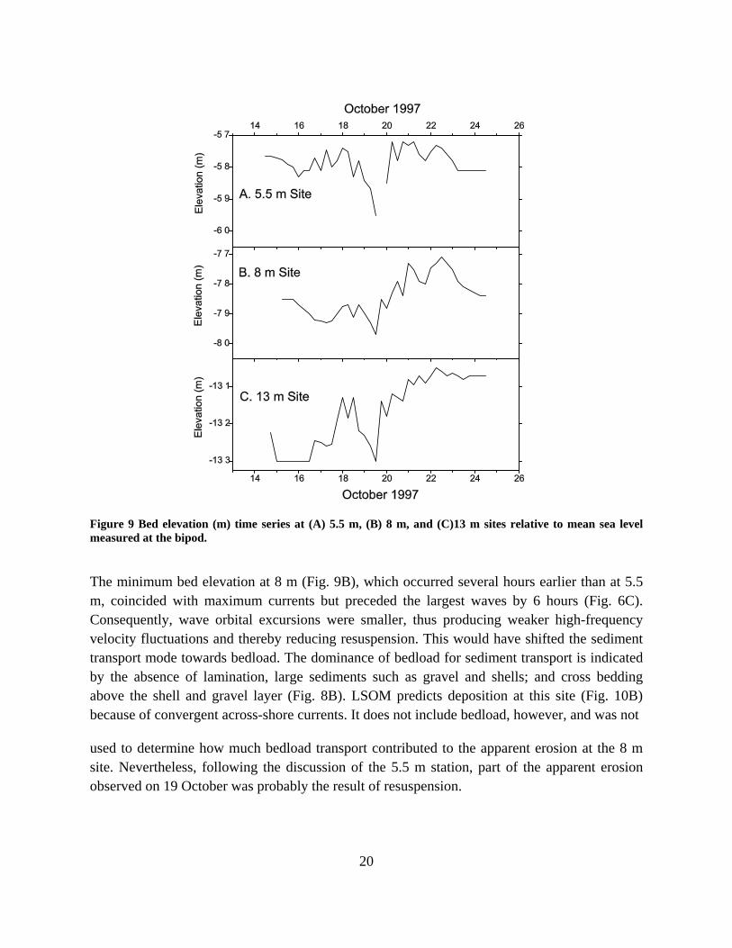
Figure 9 Bed elevation (m) time series at (A) 5.5 m, (B) 8 m, and (C)13 m sites relative to mean sea level measured at the bipod.

The minimum bed elevation at 8 m (Fig. 9B), which occurred several hours earlier than at 5.5 m, coincided with maximum currents but preceded the largest waves by 6 hours (Fig. 6C). Consequently, wave orbital excursions were smaller, thus producing weaker high-frequency velocity fluctuations and thereby reducing resuspension. This would have shifted the sediment transport mode towards bedload. The dominance of bedload for sediment transport is indicated by the absence of lamination, large sediments such as gravel and shells; and cross bedding above the shell and gravel layer (Fig. 8B). LSOM predicts deposition at this site (Fig. 10B) because of convergent across-shore currents. It does not include bedload, however, and was not

used to determine how much bedload transport contributed to the apparent erosion at the 8 m site. Nevertheless, following the discussion of the 5.5 m station, part of the apparent erosion observed on 19 October was probably the result of resuspension.

21

The time series of bed elevation at 13 m indicates deposition on 18 October, but this sediment was removed by the SandyDuck storm and a new bed was deposited. The lower contact of the SandyDuck storm bed (Fig. 8C) is not a scour surface as at 5.5 m but it is more distinct than at 8 m. The dominant mode of deposition at 13 m varied continuously between bedload and suspended load through 20 October (Beavers 1999). Continuous deposition at this depth is implied by the consistent convergent flow regime; seaward velocities were negligible at this mooring during the storm whereas offshore flow was strong at 8 m. Given the available observations and model results (Figs. 8C and 10C), it seems likely that the minimum bed elevation here was also caused by resuspension.

Figure 10. Time series of bed elevation predicted by LSOM using currents that increase southward (erosional currents) at (A) 5.5 m, (B) 8 m, and (C)13 m sites. The solid squares are the observations.

22

3.4 Sediment fluxes and mass conservation

Across-shore sediment transport is forced by waves and steady currents. (Ruessink, Houwman et al. 1998) concluded that the mean flow is not important for water depths shallower than 6 m, whereas the mean flow dominates offshore fluxes during storms in 7-17 m depths in the Middle Atlantic Bight (Wright, Boon et al. 1991). Wright et al. further reported that incident waves cause both shoreward and seaward fluxes under all conditions, whereas mean currents cause both shoreward and seaward fluxes during moderate to fairweather conditions only. Based on observations of sediment transport on the Long Island shoreface, (Swift, Niedorida et al. 1985) suggested that shoaling long waves continuously transport sediment landward during fair-weather-to-moderate conditions when either upwelling or downwelling coastal currents prevail. It is also of interest that quasi-steady near-bottom flow dominates seaward bar migration in water depths less than 8 m at the study site (Thornton, Humiston et al. 1996; Gallagher, Elgar et al. 1998).

Table 1. Net bed-elevation profile change during the SandyDuck storm.

1D currents;

Closed BC

1D Currents;

Open BC

2D

Depositional

Currents; Open

BC

2D Erosional

Currents; Open

BC

Measured at

5.5 m, 8 m, and

13 m sites

Net change (m) 0.00 -0.89 0.15 0.08 0.15

3.4.1 Seaward transport

Waves and mean currents worked in combination to transport sediment seaward during the field study. The peak period during the storm increased from less than 7 s to more than 10 s while the wave height was also increasing (Fig. 6). The incident waves at the FRF before and after the storm had peak periods > 10 s and significant wave heights < 2 m, which would have driven shoreward bed load transport. The measured seaward mean flow exceeded 0.1 m s-1 at the 8 m bipod while offshore flow was irregular at the other locations (Fig. 7). Seaward transport by unsteady flow in the surf zone would have prevailed at 5.5 m but the weak seaward flow at 13 m suggests that sediment exchange with the inner shelf would have been limited. Table 1 does not list results for alongshore currents that either erode or deposit with closed boundaries

23

because the results were unrealistic. Even with very weak gradients, several meters of sediment were deposite and/or eroded across the entire shoreface.

Treating the boundaries as closed for no net alongshore transport did produce reasonable results at the measurement sites (not shown). However, sediment deposited at the seaward margin of the model grid (Fig. 11A) could have constructed a large bar (> 1 m). The prediction of such a large storm deposit at the seaward margin of the FRF by the numerical model suggests that some exchange must have occurred. The observed mean flow also produces an event bed on the shoreface in the numerical model for all cases (Fig. 11). This uniform distribution is in general agreement with other observations, which do not show sandbar formation at depths of 8-13 m.

Figure 11.Model-predicted depth profiles during the SandyDuck storm in 1997: (A) no along-shore change in currents and a closed seaward boundary; (B) with decreasing alongshore currents and an open seaward boundary.

3.4.2 Alongshore transport

Several processes contribute to alongshore sediment transport within the Middle Atlantic Bight. Waves approaching the beach obliquely drive longshore currents within the surf zone. Coastal jets, such as that originating at the mouth of Chesapeake Bay, also drive southward alongshore flow within the FRF area. During storms, elevated water levels at the coast generate a seaward pressure gradient that drives alongshore flow on the inner shelf. These mechanisms generated

24

alongshore velocities that were significantly stronger than across-shore velocities during the instrument deployment, especially during the SandyDuck storm (Fig. 7). Alongshore currents indirectly impact bar formation by interacting with infragravity waves, which are influenced by the across-shore structure of the alongshore flow (Howd, Bowen et al. 1992). Alongshore currents also directly cause deposition and erosion through alongshore variations in the sediment transport rate. This effect is commonly neglected in studies of bar migration, thus permitting the use of one-dimensional models to predict beach profile evolution. However, the standard deviation of the alongshore flow is of order 0.1 m s-1 on the upper shoreface (Thornton, Humiston et al. 1996). The alongshore velocity gradient of 0.03 m s-1 used in this study is thus reasonable. Seaward transport is also supported by observations of the discrete sediment lobes that are deposited by coastal jets during downwelling (Wright, Boon et al. 1986). If this source of sediment is not accounted for, there will be an apparent across-shore sediment flux from the shoreface to the beach face. Such an alongshore sediment flux may partially account for the failure of energetic-based models to recover the beach profile when waves are not the dominant forcing.

The alongshore velocity gradient causes suspended sediment transport rate magnitudes to decrease as well and consequently the transport vectors became progressively more seaward to the south. The predicted profiles (Fig. 11) are taken from 750 m north. The transport field along this line indicates erosion landward of 6 m and deposition seaward; the landward erosion is greater than 50 cm and a sand layer is spread over a wide area on the shoreface. This profile should be near the neutral section for erosion/deposition associated with the alongshore transport gradient.

The final bed elevation at 5.5 m (Fig. 10A) is 0.06 m high and that at 8 m is 0.17 m high (Fig. 10B) whereas the model predicts the final elevation at the 13 m station well. The model is not expected to accurately predict the bed elevation history during the observation period because it only includes the mean near-bottom flow, which is interpolated from a limited number of measurements. Nevertheless, Figures 10 and 11 demonstrate that an updrift source of sand can balance sediment lost to the inner shelf. Furthermore, because of erosion and secondary flows induced by wave breaking in shallow water, it is reasonable that the model does not reproduce the measured final bed elevation at the 5.5 and 8 m sites.

4 Coastal hydrodynamics and potential erosion

Hurricane Isabel made landfall on the Outer Banks of North Carolina (Fig. 12) at 1100 UT on 18 September 2003 (Keen, Rowley et al. 2005). The National Oceanic and Atmospheric Administration (NOAA) flew several reconnaissance flights over the barrier islands afterward to assess the damage. Washover terraces and perched fans were deposited 650 m inland at a

25

distance of 50 km from landfall (Ocracoke, Fig. 13A) whereas channels were eroded in addition to dune erosion and washover 60 km east of landfall (W. Hatteras, Fig. 13B). At a distance of 70 km from the storm track, coastal dunes were severely eroded and washover terraces, perched fans, and sheetwash lineations were deposited up to 500 m inland (Frisco, Fig. 13C). The storm impacts at ~75 km east of landfall were limited to dune erosion, and the construction of washover terraces and perched fans up to 400 m inland (Buxton, Fig. 13D).

 

 

Figure 12. Map of the Outer Banks showing the path of Hurricane Isabel on 18 September 2003. The inset map shows the Cape Hatteras locations (circled) discussed in the text.

4.1 The model system

A parametric cyclone wind model was used to calculate the wind field. The wave field was calculated by SWAN and NCOM was used to calculate ocean currents. NCOM was initialized using temperature and salinity data from a global circulation model and forced with tidal elevations and transports at open boundary points from a global tide model (Egbert, Bennett et al. 1994). The interaction of waves and currents near the seabed as well as sedimentation were represented by LSOM. All of the models used a cell size of 3.02 km and 3.71 km along the x (easting) and y (northing) axes, respectively. The bathymetry came from the DBDB2 database. The hindcast interval was 0000 UT on 16 September to 1500 UT on 19 September. The model operation sequence is: (1) the Holland wind model (Holland 1980); (2) the SWAN wave model; (3) the NCOM circulation model; and (4) the coupled BBLM and sedimentation model (LSOM).

78 W 76 W 74 W

34N

36N

34N

36N

78 W 76 W 74 W

North

C arolina

V irginia

Atlantic Ocean

Ins et

Map

Isabel T

rack

B uxton

Ocracoke

Is land

F risco

Marsh

0 - 2 m Depth

Over 2 m Depth

0 5 km

C ape Hatteras

National S eashore

P amlic o S ound

26

   

   

Figure 13. Aerial photographs taken after Hurricane Isabel on the Outer Banks (see Fig. 1B for locations). (A) Ocracoke Island; (B), Cape Hatteras National Seashore; (C) Frisco; and (D) Buxton. The photographs are oriented with Pamlico Sound to the left. The arrows indicate north.

There were few observations to validate the model system predictions for this example. No winds or wave parameters were measured near the coast. The tide gauge near the Hatteras lighthouse, which failed at the storm peak, suggests that the simulated water levels were substantially lower than observed. This is considered reasonable in light of the large cell size and lack of nearshore bathymetry, which has a strong influence on coastal setup. Overall, the lack of validation data for this exercise is acceptable because of the previous validation of the models and the general nature of the problem being addressed. For more detailed predictions validation data would be critical.

27

4.2 Potential erosion during Hurricane Isabel

The net sediment loss on the Outer Banks is consistent with the majority of published morphological data for hurricane impacts on mid-latitude coasts. It is clear from the observations that some sediment was deposited on the landward side of the islands, but the excessive erosion of the dune-beach system suggests that it was the primary source of sand for the coastal transport system.

The carrying capacity of the coastal sediment transport system can be approximated by the

potential coastal erosion (), which is the maximum volume of sediment mobilized by erosional processes (Lawrence and DavidsonArnott 1997; Ruggiero, Komar et al. 2001). The dune erosion potential can be evaluated by comparing the cross-sectional area of the dune-beach

system, AD = LHD, to the potential erosion (Fig. 14), where HD is the mean height of the dune-beach system and L is its width. The dune-beach system will be potentially removed when

AD < . When HD is unknown, as in this study, the potential for dune erosion can be estimated

by calculating the average height, HAC = /L, that would produce a beach-dune volume that is

Figure 14. Schematic of mass terms for beach erosion. See text for explanation.

equal to . The storm surge effectively reduces the dune height by . The equivalent beach

height HAC is increased by the total setup ; HAC = HAC + . For example, L is approximately 250 m at Ocracoke, 100 m at the western end of Hatteras Island, 200 m at Frisco, and 150 m at

Buxton (Table 2). The predicted values of (Fig. 15) decrease eastward; consequently, HAC = 1.04 m, 1.58 m, 0.9 m, and 0.6 m at Ocracoke, Cape Hatteras National Seashore (a larger

predicted ), Frisco, and Buxton, respectively. The morphodynamic causes of the observed erosion pattern indicate that the key parameter in causing breaching is the dynamic equivalent beach height HD, which can be defined as the sum of HAC and the pressure gradient across the

island, , which can be defined as the difference in water level on the open sea and lagoon margins.

L

HD

AD = L × HD

28

 

Figure 15. Potential erosion (m2) predicted by LSOM during Hurricane Isabel at the locations shown in Figure 1b. The distance from landfall is given in parentheses. The units are m3 of sand eroded per m of coastline.

The predicted at Ocracoke at landfall is 0.65 m (Table 2). The hindcast water level at

Hatteras National Seashore is -1.8 m and is 2.3 m. This large gradient, in combination with significant dune erosion and a narrow width (less than 250 m), allowed breaching at this location where HD is 3.88 m, which exceeds the inferred dune height from Figure 14. A similar pressure gradient is predicted at Frisco but no channel was incised, partly because of somewhat

lower dune erosion ( = 80 m2) and greater width (more than 500 m). Although the hindcast water level inside the sound is lower at Buxton (-2.4 m), the low setup on the open coast results in a difference of 2.6 m. The dunes were entirely removed but the width of the island prevented

breaching despite the large .

The observed water levels during Hurricane Isabel (measured < 2 m) did not exceed the dunes on Hatteras Island and submergence would have been unlikely. Therefore, for channel incision to occur, the dune-beach system must first have been substantially eroded by waves. The predicted waves along the Outer Banks were about 7 m high, which would have substantially contributed to this process. If the dunes are locally reduced by waves, the pressure gradient can drive a steady current landward that will combine with storm waves to rapidly erode a channel.

-76.2 -76.0 -75.8 -75.6 -75.40

20

40

60

80

100

120

Buxt

on

(75

km)

Frisc

o (7

0 km

)

Cape

Hat

tera

s Na

tiona

l Se

asho

re (6

0 km

)

Ocr

acok

e Is

land

(50

km)

m3 /m

West Longitude

29

Table 2. Potential erosion of the Outer Banks during Hurricane Isabel.

Location (DX) L (m) (m2) H

AC (m)

(HAC

= /L)

(m)

Ocracoke (50 km) 250 110 1.04 0.65

Hatteras Nat’l Seashore (60 km) 100 108 1.58 2.3

Frisco (70 km) 200 80 0.9 2.3

Buxton (75 km) 150 60 0.6 2.6

These results are somewhat qualitative because of a lack of beach-dune profiles, the coarse resolution of the numerical models, and the importance of several nearshore processes that are not included in these models, such as wave-driven flow and island inundation. Nevertheless, we consider these results to be robust because of their dependence on fundamental physics rather than parameterizations of diverse observations. The models predict a strong current system and large waves along the ocean side of the islands, where erosion of the inner shelf would occur if not for the supply of sand from the beach-dune sand reservoir. The comparison between the model results and the observed erosion indicates that where this sand reservoir was insufficient the dunes were removed and breaching occurred. A more detailed simulation of the timing of these erosional processes will require additional research.

5 Nearshore resuspension and optics

With increasing use of remote sensing of the coastal environment, there is an evolving need to predict the optical properties of the water column. This problem relates to the both the performance of a range of sensors (passive and active) and interpretation of the results. This research is motivated by the mine warfare community within the U.S. Navy, which is planning to deploy optical instruments operationally in the near future. NRL has been investigating the processes that relate directly to effective prediction through an ongoing basic research program that focuses on not only the sedimentological problem but also the coupling of hydrodynamics to sedimentation. Previous work has identified the key requirements for accurately predicting optical scattering in water depths shallower than 30 m for sandy coasts (Stavn and Keen 2004).

30

These properties are passed to optical sensor models in an attempt to understand what the end-user (sensor operator or interpreter) needs to know.

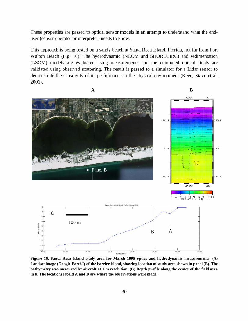
This approach is being tested on a sandy beach at Santa Rosa Island, Florida, not far from Fort Walton Beach (Fig. 16). The hydrodynamic (NCOM and SHORECIRC) and sedimentation (LSOM) models are evaluated using measurements and the computed optical fields are validated using observed scattering. The result is passed to a simulator for a Lidar sensor to demonstrate the sensitivity of its performance to the physical environment (Keen, Stavn et al. 2006).

Figure 16. Santa Rosa Island study area for March 1995 optics and hydrodynamic measurements. (A) Landsat image (Google Earth) of the barrier island, showing location of study area shown in panel (B). The bathymetry was measured by aircraft at 1 m resolution. (C) Depth profile along the center of the field area in b. The locations labeld A and B are where the observations were made.

Panel B

A B

100 m

A B

C

31

5.1 Hydrodynamic measurements at Santa Rosa Island, Florida

A field program was completed from 2-15 March 1995 by NRL to follow up an earlier optical study at this location (Gould and Arnone 1997; 1998). In addition to aircraft and in situ optical measurements, two moorings were deployed to measure currents, waves, water depth, chlorophyll, salinity, and temperature in depths of 2.7 and 4.8 m (bracketing a submerged bar). The study also measured the initial bathymetry at ~2 m resolution using an aircraft system.

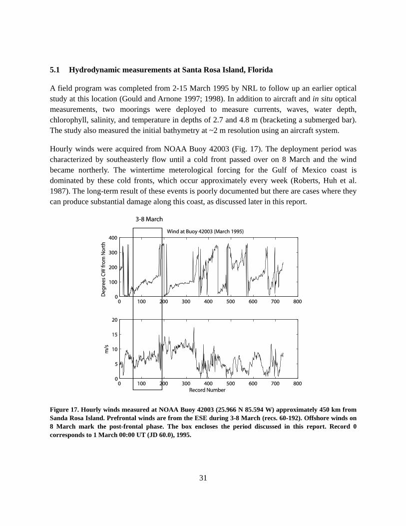
Hourly winds were acquired from NOAA Buoy 42003 (Fig. 17). The deployment period was characterized by southeasterly flow until a cold front passed over on 8 March and the wind became northerly. The wintertime meterological forcing for the Gulf of Mexico coast is dominated by these cold fronts, which occur approximately every week (Roberts, Huh et al. 1987). The long-term result of these events is poorly documented but there are cases where they can produce substantial damage along this coast, as discussed later in this report.

Figure 17. Hourly winds measured at NOAA Buoy 42003 (25.966 N 85.594 W) approximately 450 km from Sanda Rosa Island. Prefrontal winds are from the ESE during 3-8 March (recs. 60-192). Offshore winds on 8 March mark the post-frontal phase. The box encloses the period discussed in this report. Record 0 corresponds to 1 March 00:00 UT (JD 60.0), 1995.

32

The prefrontal winds strengthened for several days prior to 8 March and reached a maximum of 8 m/s before reversing direction. The onshore wind generated steady waves with heights of 1 m (Fig. 18A) until the prefrontal phase, during which wave heights increased rapidly until early

Figure 18. (A) Significant wave height (m) and (B) sea surface anomaly measured at site B. Record 1 corresponds to 0600 CST on March 3 (JD 62.25) and the record interval is 10 minutes. See Fig. 16 for location.

A

B

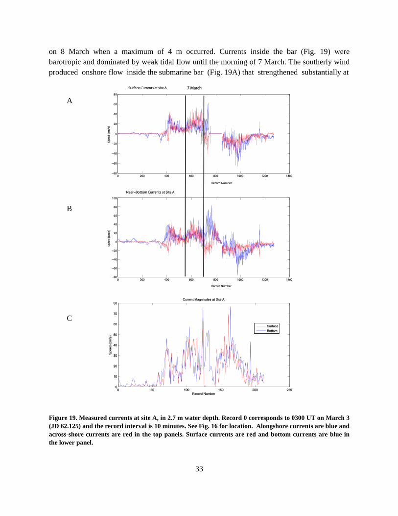
33

on 8 March when a maximum of 4 m occurred. Currents inside the bar (Fig. 19) were barotropic and dominated by weak tidal flow until the morning of 7 March. The southerly wind produced onshore flow inside the submarine bar (Fig. 19A) that strengthened substantially at

Figure 19. Measured currents at site A, in 2.7 m water depth. Record 0 corresponds to 0300 UT on March 3 (JD 62.125) and the record interval is 10 minutes. See Fig. 16 for location. Alongshore currents are blue and across-shore currents are red in the top panels. Surface currents are red and bottom currents are blue in the lower panel.

A

B

C

34

the surface (red line in Fig. 19A) while becoming more eastward near the bottom, as indicated by the positive alongshore currents (blue line in Fig. 19B). The surface currents peaked at < 50 cm/s (red line in Fig. 19C) whereas the bottom currents exceeded 70 cm/s (blue line in Fig. 19C). This eastward flow was probably caused by both the wind stress and wave breaking over the bar (see Fig. 16). A lack of turbulent mixing at this site is indicated by the temperature

measurements (Fig. 20), which remain consistently ~2C different even during the peak wind

and waves. The tidal signal is ~1 in magnitude but postfrontal cooling on 8 March produced a

2 decrease in temperature throughout the water column.

Figure 20. Temperature measured at site A (water depth = 2.7 m). Record 0 corresponds to 0300 on March 3 (JD 62.125), 1995. The horizontal axis is the record number (interval is 10 minutes). The vertical lines represent 0000 hr on March 7 and 8, thus bracketing the front discussed in the text. The red line is the temperature ~1 m below the surface and the green line is ~1 m above the bottom.

The postfrontal winds remained northerly until early on 9 March before becoming southerly again (Fig. 17). Postfrontal waves responded by decreasing to less than 0.1 m (Fig. 18A) and currents became minimal at the bottom. Unfortunately, the surface current meter did not record during this time interval. Flow at this location became westward and slightly offshore after 8 March as indicated by all current components being negative in Figs. 19A and 19B. This strong flow was probably partly forced by the nearshore sea surface anomaly associated with the front (Fig. 18B). Note the decrease of ~0.2 m immediately after the wind changed direction. Also note the even stronger front that followed that of 7-8 March, which is evidenced by the wind speed > 10 m/s (record 300 in Fig. 17) and the increasing coastal setup and wave heights in Fig. 18.

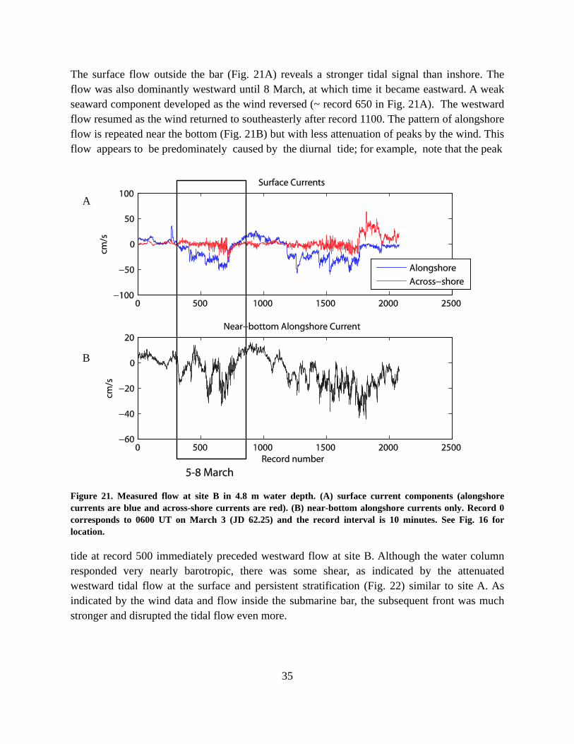
35

The surface flow outside the bar (Fig. 21A) reveals a stronger tidal signal than inshore. The flow was also dominantly westward until 8 March, at which time it became eastward. A weak seaward component developed as the wind reversed (~ record 650 in Fig. 21A). The westward flow resumed as the wind returned to southeasterly after record 1100. The pattern of alongshore flow is repeated near the bottom (Fig. 21B) but with less attenuation of peaks by the wind. This flow appears to be predominately caused by the diurnal tide; for example, note that the peak

Figure 21. Measured flow at site B in 4.8 m water depth. (A) surface current components (alongshore currents are blue and across-shore currents are red). (B) near-bottom alongshore currents only. Record 0 corresponds to 0600 UT on March 3 (JD 62.25) and the record interval is 10 minutes. See Fig. 16 for location.

tide at record 500 immediately preceded westward flow at site B. Although the water column responded very nearly barotropic, there was some shear, as indicated by the attenuated westward tidal flow at the surface and persistent stratification (Fig. 22) similar to site A. As indicated by the wind data and flow inside the submarine bar, the subsequent front was much stronger and disrupted the tidal flow even more.

A

B

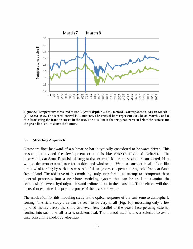
36

Figure 22. Temperature measured at site B (water depth = 4.8 m). Record 0 corresponds to 0600 on March 3 (JD 62.25), 1995. The record interval is 10 minutes. The vertical lines represent 0000 hr on March 7 and 8, thus bracketing the front discussed in the text. The blue line is the temperature ~1 m below the surface and the green line is ~1 m above the bottom.

5.2 Modeling Approach

Nearshore flow landward of a submarine bar is typically considered to be wave driven. This reasoning motivated the development of models like SHORECIRC and Delft3D. The observations at Santa Rosa Island suggest that external factors must also be considered. Here we use the term external to refer to tides and wind setup. We also consider local effects like direct wind forcing by surface stress. All of these processes operate during cold fronts at Santa Rosa Island. The objective of this modeling study, therefore, is to attempt to incorporate these external processes into a nearshore modeling system that can be used to examine the relationship between hydrodynamics and sedimentation in the nearshore. These effects will then be used to examine the optical response of the nearshore water.

The motivation for this modeling study is the optical response of the surf zone to atmospheric forcing. The field study area can be seen to be very small (Fig. 16), measuring only a few hundred meters across the shore and even less parallel to the coast. Incorporating external forcing into such a small area is problematical. The method used here was selected to avoid time-consuming model development.

37

Global non-tidal flow, sea surface anomalies, temperature, and salinity fields for the Florida

coast were taken from the 1/8 global NCOM fields for 1995. These fields were passed to a regional model with a grid cell size of 300 m. The astronomical tides were added to this model’s open boundaries from the Oregon State tidal model (Martin, Smith et al. 2009). This grid included the Mobile, Escambia, and Choctawhatchee Rivers, as well as Econfina Creek. The calculated currents, temperature, salinity, and water levels from this grid were used as boundary conditions for a smaller nest with a cell size of ~100 m, which used the same wind forcing but included no rivers. The computed fields from this model were then passed to a one-way nested model on the grid shown in Fig. 16, which had a cell size of 10 m. The wind forcing for both nested models was taken from NOAA buoy 42003 (Fig. 17).

The wave-driven flow within the inner nest was computed using SHORECIRC on a 10 m grid. This version of SHORECIRC does not include wind or tidal forcing and it must use periodic boundaries at the across-shore edges of the domain. However, it is coupled to SWAN and can thus calculate local wave generation in addition to incident swell waves from offshore. The seaward wave properties for SWAN included time series of wave height, periods and directions (JONSWAP spectrum assumed). The resulting radiation stresses were summed over the spectrum and used for nearshore forcing of SHORECIRC. SHORECIRC included both the standard and roller-enhanced radiation stress inputs, and a mass flux from Stokes drift and rollers to calculate the undertow/3D current profile.

The currents calculated from SHORECIRC and NCOM were superimposed to produce 3D fields that reflect both local and far-field forcing. These currents were used by LSOM to calculate wave-current shear stresses, sediment entrainment, and erosion-depositon on the shoreface. The resulting suspended sediment fields were used to calculate optical scattering fields. Finally, the scattering was passed to a laser simulator to examine the potential impact on electro-optical mine-hunting sensors. The simulation covers 1-15 March 1995.

5.3 Simulated hydrodynamics

The hydrographic predictions from the numerical models can be validated using the

observations at sites A (30.385 N) and B (30.384 N), both of which are located at a longitude

of 86.803 W. The separate model output will first be examined before discussing the combined results. This will permit specific model-related problems to be evaluated. The global model will not be examined because it does not extend to the coast.

5.3.1 NCOM simulations

The 100 m grid can be examined using a grid cell from (30.3823N, 86.8044W), which is the closest wet cell to the study area. The across- and along-shore components of the surface currents at site B (Fig. 23) reveal how well NCOM did. The match in both magnitudes and

38

Figure 23. Comparison of 100 m NCOM results and observations. Timeseries of (A) along-shore and (B) across-shore surface currents at site B during March 1995.

phase is actually quite good considering the use of winds from ~450 km distant and the 100 m resolution of the NCOM grid. The most obvious problem with the along-shore currents is that they are too strong during the prefrontal winds. For example, the observed alongshore flow for JD 63-65 (4-6 March) reversed from weakly eastward (positive values for red line in Fig. 23A) to westward while NCOM remained westward with magnitudes as high as 40 cm/s. This is very likely caused by using the buoy winds, which were from the SE during this interval (Fig. 17). The predicted and observed along-shore currents are in reasonable agreement through JD 67.9, when the front passed over. The buoy winds used to force NCOM quickly returned to SE and so the model currents returned to westward before the observations. The pattern of increasing westward surface flow is consistent, however. The across-shore currents were weak except during the rapid rotation of the wind on JD 67 (Fig. 23B). The model reproduces this rapid reversal well but offshore flow (< 0 in Fig. 23B) is too strong for JD 68-70 (9-11 March). The observations indicate no across-shore flow at this time. There is no purpose in evaluating the currents at site A because the model resolution includes both moorings. Overall, the model has done a good job at this location and can be considered reasonable for examining general flow along this coast. It remains to be seen how much wave-driven flow contributed to the measurements. For this we will examine the SHORECIRC results but, first, we will briefly examine flow on the outer and inner nests for NCOM.

A

B

39

The outer nest (300 m) at site A can be evaluated using a cell at (30.3751N, 86.7941W), which is at the edge of the wet domain. The main difference between these simulated currents (Fig. 24) and those from the 100 m nest is the offshore flow immediately after the front. The along-shore current (Fig. 24A) during JD 68 (9 March) is decreased and is closer to the observations but the across-shore component (Fig. 24B) has increased substantially and is not as good as the smaller nest. This is an expected result because the 300 m nest places this mooring at the boundary, which is represented by a 1 m wall in the model. This will tend to enhance across-shore motion.

Figure 24. Comparison of 300 m NCOM results and observations at Site B. Timeseries of (A) along-shore and (B) across-shore surface currents at site B during March 1995.

An inner nest of the same size as the bathymetry measurements from the field study was also used in order to ascertain the restrictions imposed by such a high resolution simulation with NCOM. The results from this 10 m nest can be reasonably compared at the two moorings. The along-shore flow at site A (Fig. 25A) shows some attenuation of the tidal signal during frontal passage on JD 65-67 (6-8 March) but the across-shore currents (Fig. 25B) are dominated by the tidal flow. This result is not as poor as it may appear, however, because the available observations (red lines) also show a strong tidal signal but with a great deal of noise that is absent from the model. The weak westward flow can also be attributed to the buoy winds as

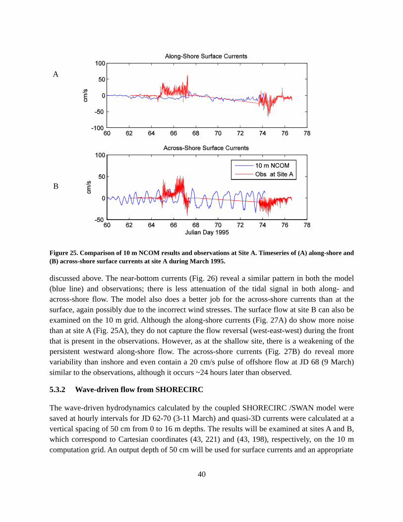
40

Figure 25. Comparison of 10 m NCOM results and observations at Site A. Timeseries of (A) along-shore and (B) across-shore surface currents at site A during March 1995.

discussed above. The near-bottom currents (Fig. 26) reveal a similar pattern in both the model (blue line) and observations; there is less attenuation of the tidal signal in both along- and across-shore flow. The model also does a better job for the across-shore currents than at the surface, again possibly due to the incorrect wind stresses. The surface flow at site B can also be examined on the 10 m grid. Although the along-shore currents (Fig. 27A) do show more noise than at site A (Fig. 25A), they do not capture the flow reversal (west-east-west) during the front that is present in the observations. However, as at the shallow site, there is a weakening of the persistent westward along-shore flow. The across-shore currents (Fig. 27B) do reveal more variability than inshore and even contain a 20 cm/s pulse of offshore flow at JD 68 (9 March) similar to the observations, although it occurs ~24 hours later than observed.

5.3.2 Wave-driven flow from SHORECIRC

The wave-driven hydrodynamics calculated by the coupled SHORECIRC /SWAN model were saved at hourly intervals for JD 62-70 (3-11 March) and quasi-3D currents were calculated at a vertical spacing of 50 cm from 0 to 16 m depths. The results will be examined at sites A and B, which correspond to Cartesian coordinates (43, 221) and (43, 198), respectively, on the 10 m computation grid. An output depth of 50 cm will be used for surface currents and an appropriate

B

A

41

Figure 26. Comparison of 10 m NCOM results and observations at site A. Timeseries of (A) along-shore and (B) across-shore near-bottom currents at site A during March 1995.

level will be used for near-bottom currents, which were measured at 1 mab. In order to avoid bottom contamination, the near-bottom currents at site A are taken from cell (32, 221) where the bar is slightly narrower in the prestudy bathymetry.

Figure 27. Comparison of 10 m NCOM results and observations at site B. Timeseries of (A) along-shore and (B) across-shore surface currents at site B during March 1995.

42

The predicted surface flow at site A (Fig. 28) suggests that the incident waves were insufficient to drive strong currents inside the bar. Waves reached their maximum height on 8 March (JD 67) when the wind was southeasterly (Fig. 17) but no mean westward alongshore flow is evident in the measured (Fig. 28B) or predicted currents (Fig. 28A). The model does predict a mean offshore surface flow of < 5 cm/s during JD 65-68 (6-8 March), which is consistent with the measured seaward flow (red line in Fig. 28B) at JD 65.0 (6 March 0000h) and ~67.1 (8

Figure 28. Alongshore (blue) and across-shore (red) surface currents at site A: (A) calculated by Shorecirc and (B) Observed.

March 0220h). The magnitudes are much weaker than observed, however. The model-predicted alongshore bottom currents (Fig. 29A) are weak and erratic but generally westward whereas the observed bottom currents (blue line in Fig. 29B) were ~30 cm/s to the east until the waves reached a maximum. The across-shore flow (red lines in Fig. 29) from SHORECIRC is more consistent with the observations. Bottom currents are seaward while waves are increasing from JD 64.5-68 (5 March 1200h to 9 March 0000h) but the magnitudes are < 2 cm/s.

The predicted surface currents at site B (Fig. 30A) are much stronger than inside the bar. The alongshore flow during the prefrontal phase (JD 64-67) is westward at ~5 cm/s, which is consistent with the SE wind direction. It is also consistent with the observed currents (Fig. 30B) but not as strong. The model across-shore flow (red line) is onshore during this interval at < 20 cm/s whereas the measured across-shore currents reverse direction more and are generally under 10 cm/s. This overall consistency also occurs during the rest of the record. Note, however, that both the model and observed across-shore currents are landward (~20 cm/s) after

B

43

Figure 29. Alongshore (blue) and across-shore (red) near-bottom currents at site A: (A) calculated by Shorecirc and (B) Observed.

JD 74 (15 March). This is also consistent with the increasing wind speed at that time (Fig. 17, record 300+).

Figure 30. Alongshore (blue) and across-shore (red) surface currents at site B: (A) calculated by Shorecirc and (B) Observed.

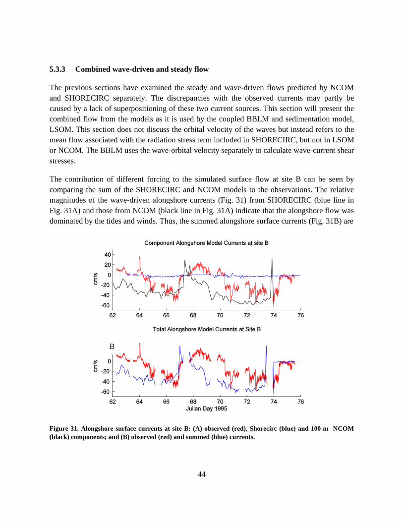
44

5.3.3 Combined wave-driven and steady flow

The previous sections have examined the steady and wave-driven flows predicted by NCOM and SHORECIRC separately. The discrepancies with the observed currents may partly be caused by a lack of superpositioning of these two current sources. This section will present the combined flow from the models as it is used by the coupled BBLM and sedimentation model, LSOM. This section does not discuss the orbital velocity of the waves but instead refers to the mean flow associated with the radiation stress term included in SHORECIRC, but not in LSOM or NCOM. The BBLM uses the wave-orbital velocity separately to calculate wave-current shear stresses.

The contribution of different forcing to the simulated surface flow at site B can be seen by comparing the sum of the SHORECIRC and NCOM models to the observations. The relative magnitudes of the wave-driven alongshore currents (Fig. 31) from SHORECIRC (blue line in Fig. 31A) and those from NCOM (black line in Fig. 31A) indicate that the alongshore flow was dominated by the tides and winds. Thus, the summed alongshore surface currents (Fig. 31B) are

Figure 31. Alongshore surface currents at site B: (A) observed (red), Shorecirc (blue) and 100-m NCOM (black) components; and (B) observed (red) and summed (blue) currents.

B

45

indistinguishable from the NCOM currents alone. The across-shore flow (Fig. 32) was more mixed and thus variable in both direction and magnitude. One consequence is that when the SHORECIRC and NCOM currents have opposite direction, the net result can be almost no flow. Note that the NCOM currents from the 100 m grid are used in the figures because these are considered to be the best solution. The location is thus approximate as discussed above. The currents calculated by SHORECIRC and NCOM were combined for use in LSOM as follows. The NCOM currents on the 100 m grid were interpolated to 1 mab and then interpolated to the 10 m grid that was used for SHORECIRC and LSOM. These currents were then added to those from 1 mab computed by SHORECIRC. The resulting combined near-bottom flow at site A is not realistic and cannot be directly compared to the near-bottom observations because of the discrepancies between the 100 m and 10 m grids. Furthermore, the total modeled near-bottom currents cannot be evaluated at site B because there are no across-shore observations.

Figure 32. Across-shore surface currents at site B: (A) observed (red), Shorecirc (blue) and 100-m NCOM (black) components; and (B) observed (red) and total model (blue) currents.

The combined flow is unavailable along the Santa Rosa Island shoreline because of the small size of the SHORECIRC domain. Nevertheless, it is instructive to examine the far-field

B

A

46

hydrodynamics because of their apparent importance during the study interval. This will be done using plots of the NCOM-computed flow on the 100 m grid, which can be reasonably applied to site B only, since there is no submarine bar in this grid. The surface currents at site B predicted by the 100 m NCOM simulation (Fig. 23) are consistent with the observations between JD 66 and 70 (7-11 March). The model predicts the return to westward flow too early, but this is a reasonable shortcoming in light of the wind forcing that was used. The following discussion will thus focus on the currents along the coast during this period, which represents a complete cold front cycle.

The predicted flow on the inner shelf was westward with mean surface currents of ~50 cm/s on 7 March (Fig. 33A). This prefrontal flow was caused by the winds from the ESE (Fig. 17). The

Figure 33A. Snapshots of currents calculated by NCOM on the 100 m grid at JD 66.125 (7 March 0300 UT). (A) Vertical perspective plot of surface current vectors over magnitude centered at 86.8 W lon, 30.33 N lat.

flow is sufficiently uniform in map view to be examined using vertical sections through the study area. The alongshore flow (Fig. 33B) was strongest near the surface (upper 3.5 m) near the coast with speeds of 80 cm/s but near-bottom currents were much weaker. Surface currents had an onshore component (Fig. 33C) as great as 20 cm/s and bottom flow was weakly offshore with magnitudes < 10 cm/s. This convergent flow produced ~10 cm of setup in the model (not

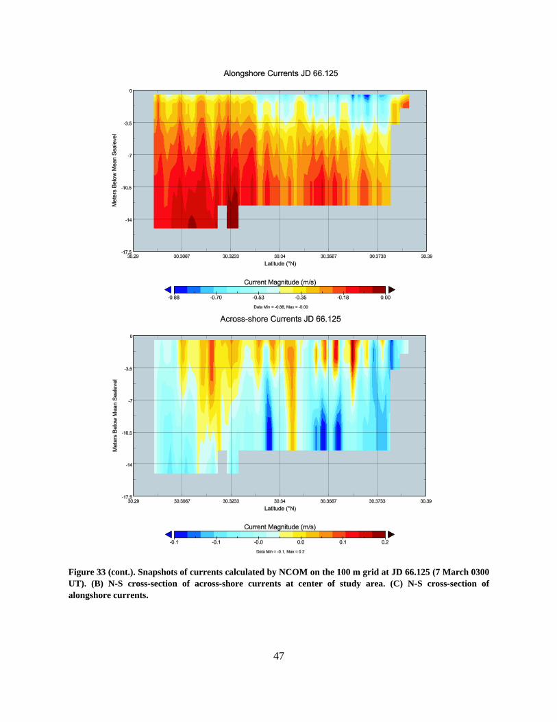
47

Figure 33 (cont.). Snapshots of currents calculated by NCOM on the 100 m grid at JD 66.125 (7 March 0300 UT). (B) N-S cross-section of across-shore currents at center of study area. (C) N-S cross-section of alongshore currents.

48

shown) during the prefrontal period. By 8 March the wind was southeasterly and the surface flow was becoming onshore (Fig. 34A), with magnitudes >50 cm/s. The alongshore component of this flow was somewhat weaker (Fig. 34B) and the mixed layer had deepened to ~5 m near the coast. In response to the increased onshore wind, across-shore flow (Fig. 34C) developed a typical downwelling-favorable regime with bottom currents as high at 20 cm/s. This flow persisted until the wind rapidly rotated to northerly late on 8 March.

Figure 34A. Snapshots of currents calculated by NCOM on the 100 m grid at JD 67.125 (8 March 0300 UT). (A) Vertical perspective plot of surface current vectors over magnitude centered at 86.8 W lon, 30.33 N lat.

The northerly winds of 9 March drove a seaward surface flow that increased in speed offshore to >50 cm/s (Fig. 35A). This flow had a weak alongshore component (Fig. 35B) that varied from 15 cm/s westward to 6 cm/s eastward, and that was uniform vertically. The seaward across-shore flow did not reach the seafloor (Fig. 35C) but reversed to onshore within a couple of meters of the bottom. Thus an upwelling-favorable flow was created by the post-frontal wind field.The northerly wind persisted for <24 hours while the predicted surface flow remained offshore (Fig. 36A) with magnitudes of ~50 cm/s. This flow had a westward component as

49

Figure 34 (cont.). Snapshots of currents calculated by NCOM on the 100 m grid at JD 67.125 (8 March 0300 UT). (B) N-S cross-section of across-shore currents at center of study area. (C) N-S cross-section of alongshore currents.

50

great as 28 cm/s at the surface while a weak eastward flow (6 cm/s) persisted at the bottom on the lower shoreface (Fig. 36B). The overall flow regime remained upwelling-favorable as indicated by near-bottom onshore currents of ~20 cm/s (Fig. 36C). Note that the offshore flow is limited to depths less than 7 m. By 11 March, the surface flow had returned to prefrontal conditions (Fig. 37A) but with slightly lower magnitudes over much of the grid. The westward component was also more broadly distributed across the shelf (Fig. 37B), reaching to the seaward edge of the model grid. The residual offshore flow remained however (Fig. 37C), in contrast to before the front (see Fig. 33C).

Figure 35A. Snapshots of currents calculated by NCOM on the 100 m grid at JD 68.125 (9 March 0300 UT). (A) Vertical perspective plot of surface current vectors over magnitude centered at 86.8 W lon, 30.33 N lat.

These NCOM results are considered to be reasonable because of their general agreement with the observations at site B. The sedimentation and optical computations resulting from them cannot be applied to the shallow site, however, for the reasons discussed above. The next section will discuss how these currents can be combined with the observed waves to predict sediment resuspension and the optical properties of the water column at this site.

51

Figure 35 (cont.). Snapshots of currents calculated by NCOM on the 100 m grid at JD 68.125 (9 March 0300 UT). (B) N-S cross-section of across-shore currents at center of study area. (C) N-S cross-section of alongshore currents.

52

Figure 36. Snapshots of currents calculated by NCOM on the 100 m grid at JD 69.125 (10 March 0300 UT). (A) Vertical perspective plot of surface current vectors over magnitude centered at 86.8 W lon, 30.33 N lat. (B) N-S cross-section of across-shore currents at center of study area.

53

Figure 36 (cont.). Snapshots of currents calculated by NCOM on the 100 m grid at JD 69.125 (10 March 0300 UT). (C) N-S cross-section of alongshore currents.

Figure 37. A. Snapshots of currents calculated by NCOM on the 100 m grid at JD 70.125 (11 March 0300). (A) Vertical perspective plot of surface current vectors over magnitude centered at 86.8 W, 30.33 N.

54

Figure 37 (cont.). Snapshots of currents calculated by NCOM on the 100 m grid at JD 70.125 (11 March 0300 UT). (B) N-S cross-section of across-shore currents at center of study area. (C) N-S cross-section of alongshore currents.

55

5.4 Sedimentation and optics

The overall objective of this study is to examine the relationship between the physical forcing and the resulting optical field in the nearshore environment. There are many factors that contribute to these processes but the observations and modeling have reduced their complexity to aid in understanding them. Mineral particles are assumed to be nonabsortive whereas the absorption by organic molecules can be parameterized using chlorophyll concentrations (Weidemann, Stavn et al. 1995). We thus neglect absorption for our purposes.

5.4.1 Bio-optical measurements

In addition to the hydrographic data discussed above, the field measurements also included pigments (chlorophyll a and pheophytin), particle numbers and their size modes (Table 3). The chlorophyll-a concentration [Chl] is used to estimate the scattering from water, phytoplankton, and organic detritus (Keen and Stavn 2000). The observed particles had very small modes (1.25

to 4.92 m), which are much too small to be sand grains or clay flocs. The mean size of

individual clay crystals is ~5 m but they are almost always found as aggregates (flocs) in oceanic waters. We assume that the total scattering BT field as measured by an instrument is given by:

bT = bw + bp + bd + bq , (1)

where: bw, bp, bd and bq are water, phytoplankton, organic detritus, and inorganic (quartz-like) scattering. We find the total organic scattering by:

bT,o = 0.21×[Chl]0.62, (2)

which is applicable to open ocean (type 1) water with no quartz. This term represents bw + bp + bd. We can then calculate the value of bq by subtracting bT,o from measurements of bT from an AC-9 optical device. This equation is used in the standared NRL model for a frequency of 440 nm (Weidemann, Stavn et al. 1995).

The most useful data from Table 3 for comparison with predictions from the models were collected along Line D at stations 3 and 4, and for 6 (1800 h) to 10 March. This is the interval for which NCOM had the best results. The beam attenuation coefficients for absorption and scattering were measured at site B (Fig. 39), which is near stations 3 and 4 (see Fig. 38). All of the optical lines should be nearly identical with respect to these parameters, however, because longshore variability should be minimal for the short distances between lines. The height of the observations above the bed was ~ 1 m. This height can be used to limit which entries from Table 3 can be used to estimate the inorganic scattering, bq. However, because of the limited data availability, we may need to compromise in this respect.

56

Table 3. Particle data collected at Santa Rosa Island, Florida, in March 1995.

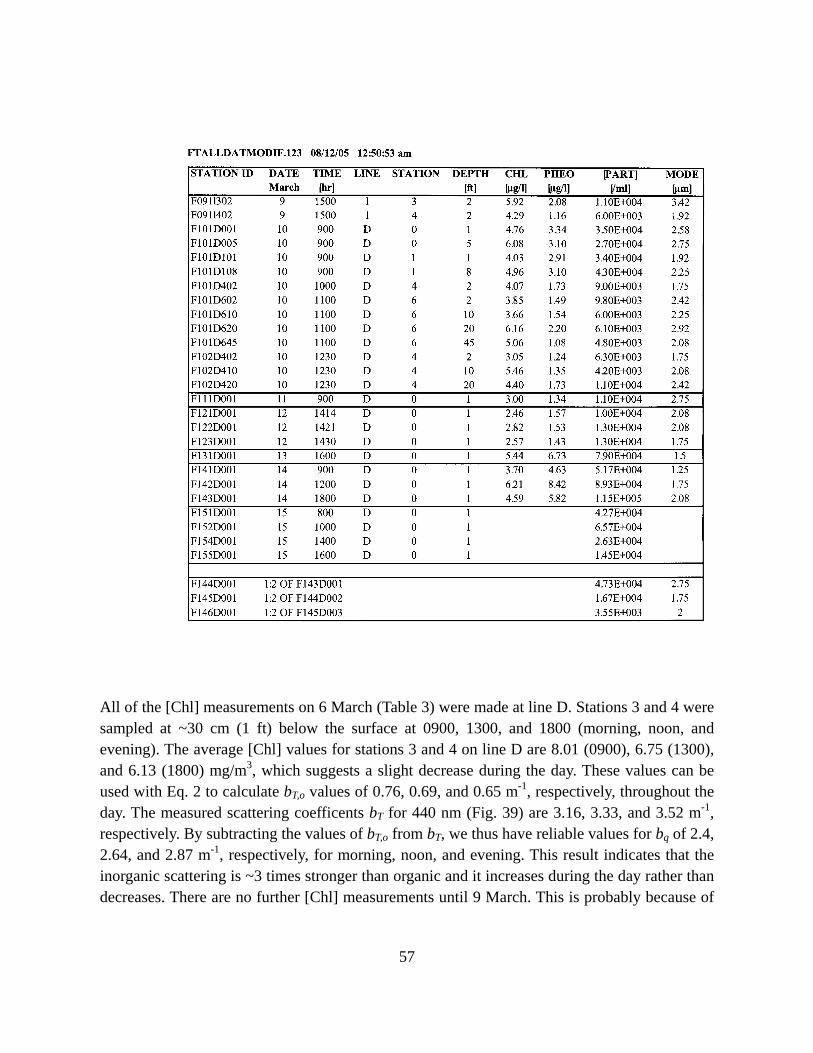
57

All of the [Chl] measurements on 6 March (Table 3) were made at line D. Stations 3 and 4 were sampled at ~30 cm (1 ft) below the surface at 0900, 1300, and 1800 (morning, noon, and evening). The average [Chl] values for stations 3 and 4 on line D are 8.01 (0900), 6.75 (1300), and 6.13 (1800) mg/m3, which suggests a slight decrease during the day. These values can be used with Eq. 2 to calculate bT,o values of 0.76, 0.69, and 0.65 m-1, respectively, throughout the day. The measured scattering coefficents bT for 440 nm (Fig. 39) are 3.16, 3.33, and 3.52 m-1, respectively. By subtracting the values of bT,o from bT, we thus have reliable values for bq of 2.4, 2.64, and 2.87 m-1, respectively, for morning, noon, and evening. This result indicates that the inorganic scattering is ~3 times stronger than organic and it increases during the day rather than decreases. There are no further [Chl] measurements until 9 March. This is probably because of

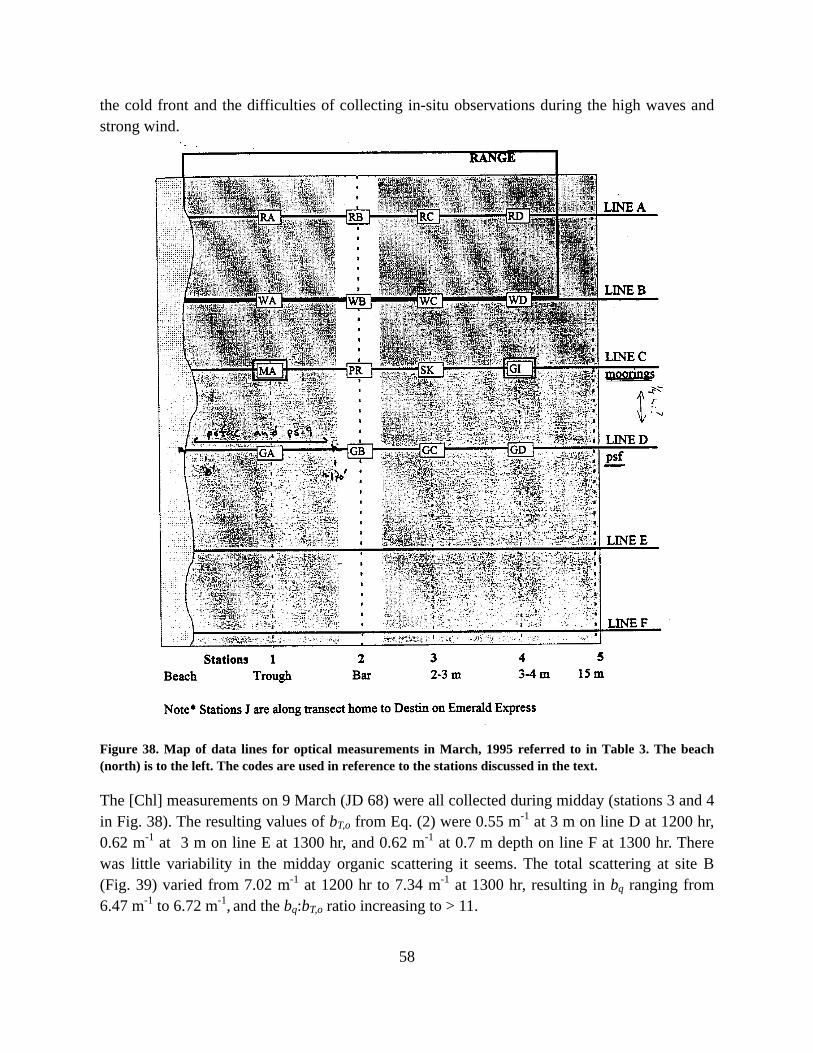
58

the cold front and the difficulties of collecting in-situ observations during the high waves and strong wind.

Figure 38. Map of data lines for optical measurements in March, 1995 referred to in Table 3. The beach (north) is to the left. The codes are used in reference to the stations discussed in the text.

The [Chl] measurements on 9 March (JD 68) were all collected during midday (stations 3 and 4 in Fig. 38). The resulting values of bT,o from Eq. (2) were 0.55 m-1 at 3 m on line D at 1200 hr, 0.62 m-1 at 3 m on line E at 1300 hr, and 0.62 m-1 at 0.7 m depth on line F at 1300 hr. There was little variability in the midday organic scattering it seems. The total scattering at site B (Fig. 39) varied from 7.02 m-1 at 1200 hr to 7.34 m-1 at 1300 hr, resulting in bq ranging from 6.47 m-1 to 6.72 m-1, and the bq:bT,o ratio increasing to > 11.

59

The most useful [Chl] measurements on 10 March (JD 69) were made on line D at station 4. At 1000 hr, the total organic scattering was 0.50 m-1 at 0.7 m below the surface and at 1230 hr a value of 0.60 m-1 is obtained from (2) at 3 m depth. The observed values of bT at site B (Fig. 39) were 3.92 and 3.41 m-1, respectively, at these same times. The resultant bq values of 3.42 and 2.81 indicate that the ratio of inorganic to organic scattering has decreased to < 5.

Figure 39. Attenuation coefficients (m-1) for absorption (blue line) and scattering (red line) at site B for 440 nm in March 1995. The AC-9 meters were at ~ 1 mab.

The scattering data discussed above indicate a pattern that can be correlated with environmental forcing. The organic scattering is relatively constant on all three days discussed and with a weak pattern on 6 March. This pattern is consistent with the fine-particle data collected simultaneously (Table 3). For example, the average number of particles on 6 March was 1.98×104 particles/ml. The concentration had decreased to 0.93×104 particles/ml by 9 March, and finally reached a minimum of 0.65×104 particles/ml on 10 March. The significant reduction between 6 and 9 March was probably the result of turbulence and strong currents destroying and removing phytoplankton cells from the nearshore during the cold front, assuming these fine

60

particle were actually phytoplankton cells. We can check this assumption by examining the size

data from Table 3. The mode for 6 March was 2.17 m (10-6 m). The mode decreased to 2.08

m by 9 March and again to 1.91 m by 10 March. A decrease in particle size during the cold front is consistent with the decrease in [Chl] and bT,o discussed above. The dominance of

phytoplankton cells < 5 m following the spring bloom has been noted in temperate nearshore environments (Tamigineaux, Legendre et al. 1999). Thus, it would seem that the waves and currents during the cold front reduced the phytoplankton population in the study area while quartz resuspension and scattering increased in response to this same forcing.

The optical properties of this same study area were measured in August 1994 and different results were found (Gould and Arnone 1997). The total scattering measured by an AC-9 at 1 mab in a water depth of 3 m, inside the bar as in this study, was more irregular and remained less than 0.7 m-1 with an average below 0.5 m-1. It is also of interest to note that profiles of scattering made at that time revealed a slight decrease from ~0.8 m-1 at the surface to < 0.4 m-1 near the bed in water deeper than 3 m outside the bar. This contrast in optical properties between August 1994 and March 1995 can be correlated to differences in the nearshore environment between summer and spring.

The primary meteorological events during the summer in the northern Gulf of Mexico are tropical cyclones whereas the winter and spring seasons are characterized by cold fronts that occur at weekly time scales. The August 1994 study period was free of tropical cyclones and the timeseries of optical properties thus reflect a benign environment with scattering and absorption values < 1 m-1 at all time and spatial scales. The profiles also indicate larger attenuation near the surface, which is consistent with near-surface phytoplankton growth. None of the near-bottom measurements indicate any resuspension of bed material. The optical properties of the study area were, therefore, modeled using simple equilibrium profiles because of the lack of resuspension (Gould and Arnone 1998). The optical measurements made during March 1995 reflect the atmospheric and oceanographic forcing discussed above. The resulting measured scattering coefficients (Fig. 39) were much larger than absorption; however, the absorption coefficients were also larger than in summer, probably because of the spring bloom.

5.4.2 Sedimentation and optics modeling

There are no observations of currents near the bed at site B. The model currents that will be used to compute the wave-current bottom shear stresses in LSOM cannot, therefore, be validated. We proceed nevertheless based on the consistent performance of NCOM at the surface (Figs. 31 and 32). The currents from SHORECIRC and NCOM were interpolated to 1 mab and summed for 7 March 0300h to 11 March 0300h (JD 66.125 to 70.125). The current components (Fig. 40A) were transformed into speed and direction (Figs. 40B and C) for use in LSOM. This type of plot reveals that when the bottom current was onshore, the magnitude

61

Figure 40. Combined currents at ~1 mab from Shorecirc and NCOM at site B. (A) Alongshore (blue) and across-shore (red) components. (B) Speed. (C) Direction.

decreased and didn’t increase until the flow was westward (~200). The changing wind field may have disrupted the nearshore flow pattern and caused it to become weak and erratic. This would have important consequences on the predicted scattering by quartz particles.

A

B

C

62

The measured waves at site B (Fig. 18) are combined with the bottom currents in LSOM to compute the shear stresses, suspended sediment distributions, and resulting scattering profiles every 12 hours during the cold front. The wave direction will be assumed to be N-S because the observations did not include directional wave data and the BBLM does not differentiate opposing wave directions. As an initial simulation of physical and optical processes during the study interval, LSOM was run with parameters derived from similar studies (Keen and Stavn

2000; Stavn and Keen 2004). These experiments change only the resuspension coefficient 0, which has been found to vary the most in previous studies. The environmental variables from observations and the numerical models are listed in Table 4 and the results are plotted with the observations at site B in Figure. 41.

Table 4. Parameters used in LSOM calibration (Fig. 41).

JD (1995) gam0 UB (cm/s) SWH (m) SWP USCW(cm/s)

66.125 0.002 31.72 0.8 4.8 8.50

66.625 0.0002 27.88 1.8 5.2 16.7

67.125 0.0002 21.49 2.3 5.2 21.8

67.625 0.002 13.49 0.8 6.7 8.90

68.125 0.02 5.94 0.5* 6.3 9.90

68.625 NA 11.96 0.1 7.3 0.81#

69.125 NA 14.10 0.2 3.8 1.02#

69.625 0.025 31.35 0.8 3.4 8.2

70.125 0.018 26.76 0.5 5.4 8.9

*Adjusted to next hour average to match observed SWH better. # Below the critical shear stress for the finest available sediment (2 cm/s)

The first date to be simulated (Table 4) is JD 66.125 (7 March 0300 hr). At this time the bottom currents ub exceeded 30 cm/s and waves were 80 cm with periods <5 sec. Even with these moderately benign hydrodynamic conditions, the average max shear velocity u* was 8.5 cm/s, which exceeds the critical shear velocity of the finest available sediment (2 cm/s). The model-

predicted bq matches the measured bT using 0 = 0.002. It is immediately obvious that this is not the value we should try to match but it is the value most often available because of the requirement for knowing [Chl] in order to calculate bT,o. It is instructive, therefore, to determine how well we can reproduce the observations without this knowledge.

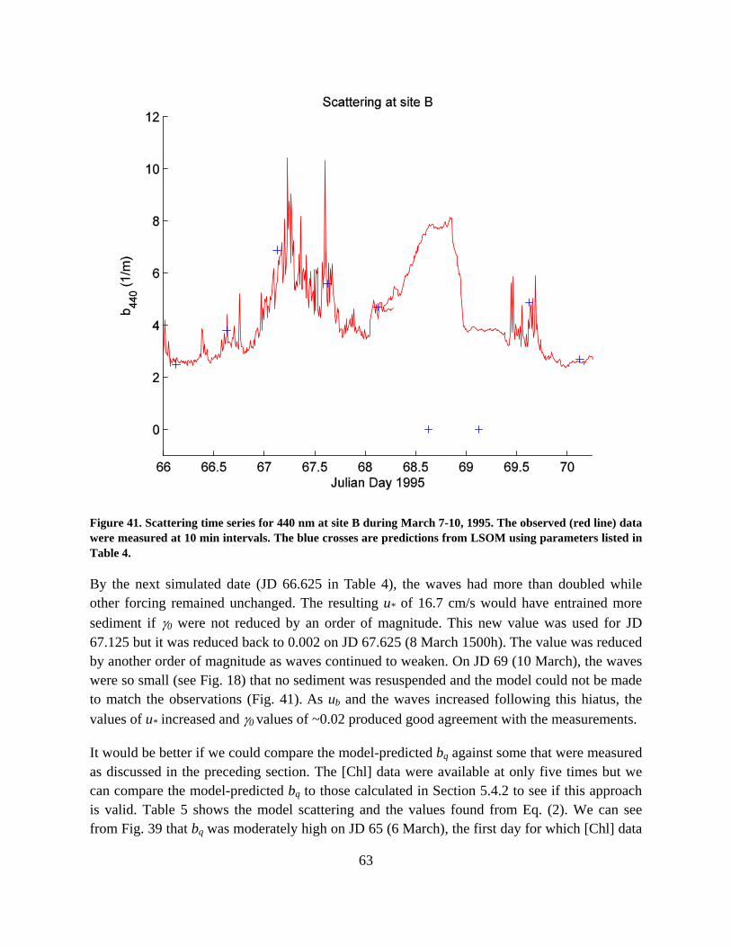
63

Figure 41. Scattering time series for 440 nm at site B during March 7-10, 1995. The observed (red line) data were measured at 10 min intervals. The blue crosses are predictions from LSOM using parameters listed in Table 4.

By the next simulated date (JD 66.625 in Table 4), the waves had more than doubled while other forcing remained unchanged. The resulting u* of 16.7 cm/s would have entrained more

sediment if 0 were not reduced by an order of magnitude. This new value was used for JD 67.125 but it was reduced back to 0.002 on JD 67.625 (8 March 1500h). The value was reduced by another order of magnitude as waves continued to weaken. On JD 69 (10 March), the waves were so small (see Fig. 18) that no sediment was resuspended and the model could not be made to match the observations (Fig. 41). As ub and the waves increased following this hiatus, the

values of u* increased and 0 values of ~0.02 produced good agreement with the measurements.

It would be better if we could compare the model-predicted bq against some that were measured as discussed in the preceding section. The [Chl] data were available at only five times but we can compare the model-predicted bq to those calculated in Section 5.4.2 to see if this approach is valid. Table 5 shows the model scattering and the values found from Eq. (2). We can see from Fig. 39 that bq was moderately high on JD 65 (6 March), the first day for which [Chl] data

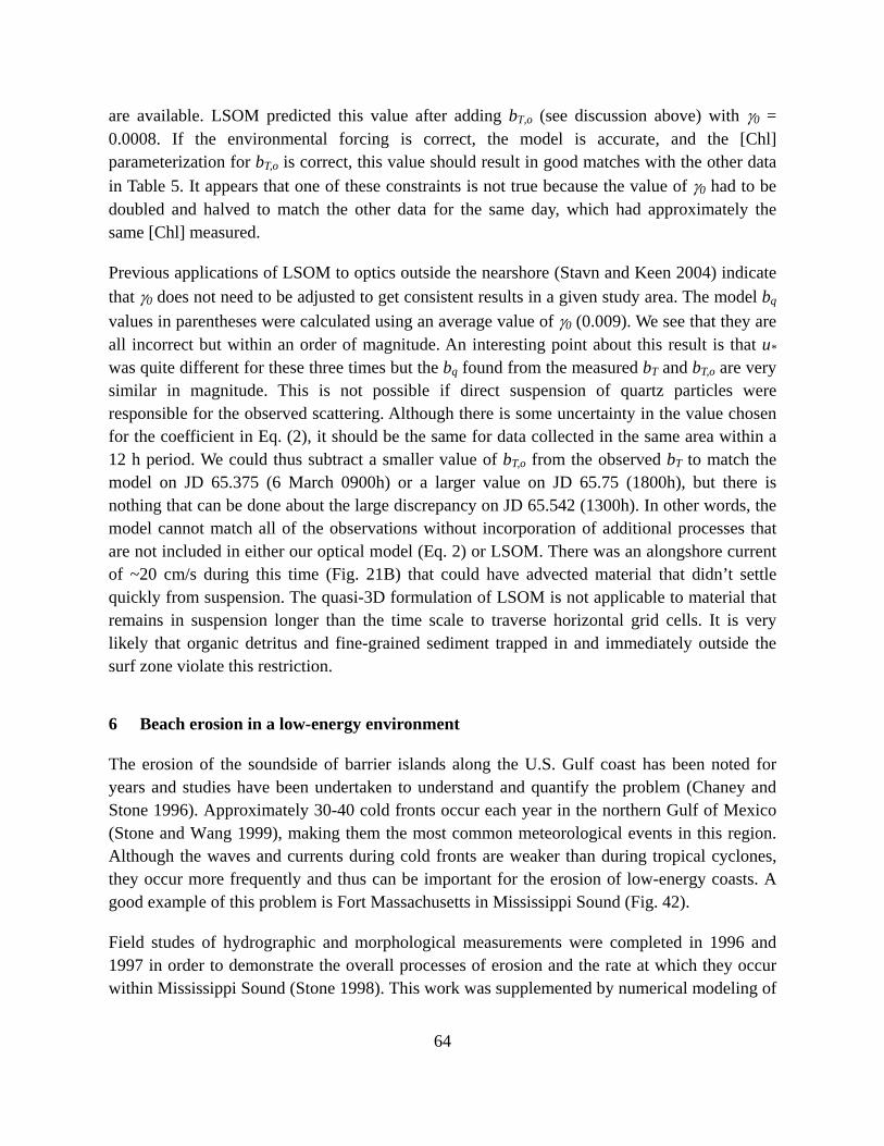
64

are available. LSOM predicted this value after adding bT,o (see discussion above) with 0 = 0.0008. If the environmental forcing is correct, the model is accurate, and the [Chl] parameterization for bT,o is correct, this value should result in good matches with the other data

in Table 5. It appears that one of these constraints is not true because the value of 0 had to be doubled and halved to match the other data for the same day, which had approximately the same [Chl] measured.

Previous applications of LSOM to optics outside the nearshore (Stavn and Keen 2004) indicate

that 0 does not need to be adjusted to get consistent results in a given study area. The model bq

values in parentheses were calculated using an average value of 0 (0.009). We see that they are all incorrect but within an order of magnitude. An interesting point about this result is that u* was quite different for these three times but the bq found from the measured bT and bT,o are very similar in magnitude. This is not possible if direct suspension of quartz particles were responsible for the observed scattering. Although there is some uncertainty in the value chosen for the coefficient in Eq. (2), it should be the same for data collected in the same area within a 12 h period. We could thus subtract a smaller value of bT,o from the observed bT to match the model on JD 65.375 (6 March 0900h) or a larger value on JD 65.75 (1800h), but there is nothing that can be done about the large discrepancy on JD 65.542 (1300h). In other words, the model cannot match all of the observations without incorporation of additional processes that are not included in either our optical model (Eq. 2) or LSOM. There was an alongshore current of ~20 cm/s during this time (Fig. 21B) that could have advected material that didn’t settle quickly from suspension. The quasi-3D formulation of LSOM is not applicable to material that remains in suspension longer than the time scale to traverse horizontal grid cells. It is very likely that organic detritus and fine-grained sediment trapped in and immediately outside the surf zone violate this restriction.

6 Beach erosion in a low-energy environment

The erosion of the soundside of barrier islands along the U.S. Gulf coast has been noted for years and studies have been undertaken to understand and quantify the problem (Chaney and Stone 1996). Approximately 30-40 cold fronts occur each year in the northern Gulf of Mexico (Stone and Wang 1999), making them the most common meteorological events in this region. Although the waves and currents during cold fronts are weaker than during tropical cyclones, they occur more frequently and thus can be important for the erosion of low-energy coasts. A good example of this problem is Fort Massachusetts in Mississippi Sound (Fig. 42).

Field studes of hydrographic and morphological measurements were completed in 1996 and 1997 in order to demonstrate the overall processes of erosion and the rate at which they occur within Mississippi Sound (Stone 1998). This work was supplemented by numerical modeling of

65

the hydrodynamics and sedimentation at Ship Island, Mississippi near Fort Massachusetts. This effort used the POM, SHORECIRC, and TRANS98 models described in Section 2 of this report. This section will descuss the observations, demonstrate the validity of the models for the problem, and the results of several numerical simulations during a cold front that occurred in March 1997. Finally, the predictions for potential erosion and transport paths during cold fronts will be discussed.

Figure 42. Ft. Mass. study area. (A) Regional map of Mississippi Sound and adjacent Gulf of Mexico. (B) Ship island, showing location of Fort Massachusetts. (C) Landsat image from GoogleEarth, showing location of pier where measurements were made (star) and erosional area to northwest of the fort.

6.1 Observations

The field deployment in late March 1997 spanned two cold fronts. The second of these, 20-21 March (JD 79-80), is discussed in this report. The wind speed at buoy 42007 (Fig. 43A) exceeded 20 m/s whereas the local wind at Ft. Massachussetts (not shown) was somewhat weaker, reaching ~12 m/s. The passage of fronts is obvious from the wind direction (Fig. 43B), which rapidly rotates from southerly to northerly. The wind does not always remain northerly

A

B C

Ship Is.

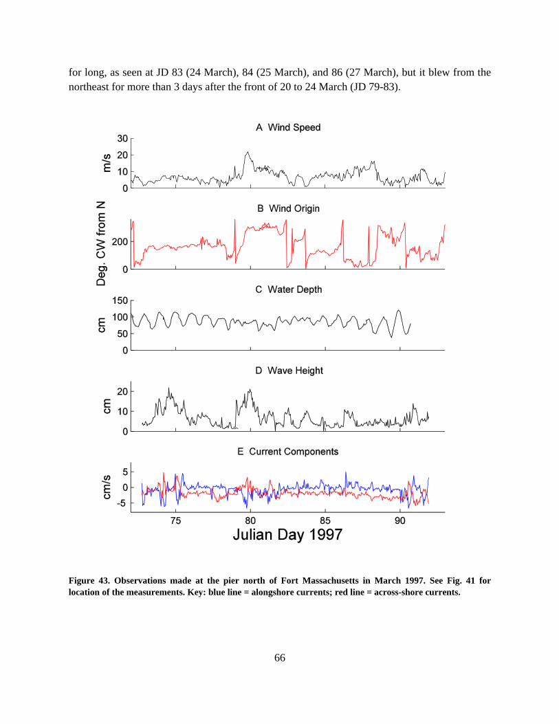
66

for long, as seen at JD 83 (24 March), 84 (25 March), and 86 (27 March), but it blew from the northeast for more than 3 days after the front of 20 to 24 March (JD 79-83).

Figure 43. Observations made at the pier north of Fort Massachusetts in March 1997. See Fig. 41 for location of the measurements. Key: blue line = alongshore currents; red line = across-shore currents.

67

The water level (Fig. 43C) was dominated by the diurnal astronomical tide but the signal was erratic when the wind was northerly (JD 79-83). The water depth at the pier was slightly elevated above the mean of 0.86 m during this period. The significant wave height HS (Fig. 43D) was low during the southerly prefrontal wind but increased to >20 cm after the front on JD 80.0 (21 March 0000h) because the wind was blowing from the northwest with maximum fetch. The waves quickly subsided, however, on 21 March and were less than 10 cm by 0600.

A peak alongshore current of –6 cm/s at West Ship Island (blue line in Fig. 43E) occurred at ~JD 79.8 (20 March 1900h) despite the northwesterly wind. Note that negative velocities are westward and southward for easting (VE) and northing (VN) currents, respectively. The flow had a northward component of 2 cm/s and was obliquely offshore to the west. This nearshore current was opposed to the wind and wave directions but consistent with the tidal flow in Mississippi Sound, which is to the west during both the flood and ebb (Keen, 2002).

Beach profiles along the soundside of Ship Island were measured at eight locations between April 1996 and June 1997 (Fig. 44). Erosion and deposition along this coast have been

Figure 44. Location of beach profiles on Ship Island measured in 1996 and 1997. See Fig. 42 for general location of Ship Island in Mississippi Sound.

discussed by (Stone 1998) and will be only briefly summarized herein. The dominant sedimentation event during the study interval was Tropical Storm Josephine, which passed southeast of Ship Island on October 7-8, 1996. Profile S1 (Fig. 45A) was located at the western end of the island, where deposition occurred throughout the year. April to October 1996 was dominated by Josephine. Even though the beach volume increased significantly by October (blue line), it is notable that offshore of 40 m was eroded by ~50 cm and post-Josephine

68

Figure 45. Measured beach profiles on the soundside of Ship Island. See Figs. 42 and 44 for location of profiles. North is to the right.

sedimentation consisted of modification of the two subaerial storm berms into a single large berm. This would have occurred by aeolian processes during northerly winds. The beach face (~0 m elevation) remained unchanged during the survey period. Profile S2 (Fig. 45B) was also characterized by depositon landward of 40 m. Erosion of the platform offshore was much

69

reduced and there was some erosion of the beach face after October 1996. This erosion was accompanied by construction of a 1 m berm on the beach. Profile S3 was located less than 500 m west of Fort Massachussetts. The offshore platform here was unchanged during the survey time but the beach prograded >30 m offshore by October 1996 (Fig. 45C). The flattened bar at ~20-30 m offshore suggests wave erosion during elevated water levels associated with Josephine. The quantity of sand deposited at this location exceeded the reworking capacity of the nearshore system and thus no berm was created by June 1997, although additional deposition on the new beach was indicated. Profile S5 was located 800 m east of Fort Massachusetts (Fig. 44) and the pattern differed from the western end of the island (Fig. 45D). Erosion between 20 and 40 m offshore was evident by October as well as on the dune landward of the beach. Further erosion occurred at the beach after October, and sediment was apparently transported onto the subaerial beach to rework the tropical storm beach into one more in equilibrium with the environment. The other profiles to the east were similar to S5.

The average beach width and volume increased 3.75 m and 2.28 m3, respectively, after Josephine because of erosion of the backshore and foredunes along the soundside coast. Following the storm, however, erosion became prevalent and the beach volume decreased substantially at most locations. Much of this erosion occurred between the October and December 1996 surveys. The profile at S8 was influenced by local sediment supply associated with overwash deposits by Josephine and the effect of wave shadowing by the recurved tip of West Ship Island.

6.2 Modeling methods and validation

6.2.1 Currents and waves

Atmospheric forcing for POM was supplied by the hourly winds measured at NOAA buoy 42007 (Fig. 43A), which is 10 km SE of Ship Island. The Naval Oceanographic Office compiled the bottom topography from a variety of sources, including the National Ocean Service 3 second database. A barotropic POM was used to examine tidal flow with an open boundary condition that included tidal elevations and depth-integrated transports from ADCIRC (Leuttich, Westerink et al. 1992). A second barotropic model was used to examine the wind-driven water levels within the region. This model used only wind forcing and closed boundaries. Finally, a barotropic POM model was used that included both tidal and wind forcing but no river inflow. The POM simulations were completed on a Cartesian grid with cells of 777 m (x axis) and 898 m (y axis). The model was spun up for 48 hours with tidal forcing only and run for the hindcast interval of 13 March to 3 April 1997 (JD 44-93). Barotropic simulations were used because of the very shallow water on the north side of Ship Island. The numerical grid used by POM was much too coarse to resolve the shallow water around Fort Massachusetts (see Fig. 42) but we can compare a nearby grid cell with the time

70

series of observations at the pier. The POM simulation did not include side friction and thus the alongshore currents (Fig. 46A) were too high. They were also dominated by the diurnal tide that occurs in the Gulf of Mexico. There are no across-shore currents in the raw model output because the numerical grid does not permit flow into landward boundaries.

Figure 46. Time series of alongshore (A) and across-shore (B) currents at the Fort Massachussetts pier (see Fig. 42 for location). (C) Water depth at the pier. Key: black= observations; blue= uninterpolated POM output; circle = Shorecirc currents; plus = total from interpolated POM and Shorecirc. The currents and water level from POM have not been interpolated and thus there is no N-S component because the output grid cell was adjacent to land.

A

B

C

71

The predicted water depth at the pier is a better fit to the data (Fig. 46C) before the front but the model continues to compute the dominant tidal elevations whereas the measurements suggest that a shorter-period oscillation occurred. This may have been caused by the preferential damping of the longer-period tidal frequencies by the offshore (southerly) wind. Furthermore, the bathymetry used in POM had a depth of 3 m instead of 1 m. The tidal signal had good phase and amplitude but the response to the frontal winds (~ 0 m depth) was stronger than measured because of the greater offshore fetch associated with the coarse bathymetry used in POM and the depth error. The wind from the buoy did not include local effects like blocking by dunes on Ship Island. The phase of the water depth response is in agreement with the observations during the initial postfrontal period but drifts off after JD 88 (29 March). The slowly increasing depth during the northerly wind between JD 80 and 85 (21 and 26 March) is reproduced well by POM, however.

The SWAN simulation for Mississippi Sound used a 69×33 km grid with 500 m resolution. Water depths were taken from POM. The uniform winds from buoy 42007 were used. No wave boundary conditions were applied at open boundaries because the model grid was almost entirely inside Mississippi Sound. The model included all shallow water physics (e.g., bottom friction). Both nonstationary and stationary runs were completed. These waves are not discussed because they were only used as boundary conditions for SHORECIRC. The waves predicted by SWAN were uniform throughout the study area with a slight eastward increase when the wind was more northwesterly.

Nearshore dynamics can be dominated by breaking waves that transfer momentum into the water column and force wave-driven currents. The SHORECIRC model simulates these currents by propagating offshore waves over the nearshore domain, calculating gradients of radiation stress (momentum flux), and using this information as a depth-integrated body force to generate the current fields. The model is quasi-3D, allowing incorporation of the dynamics inherent in depth-varying currents (in particular, enhanced dispersive mixing) without explicit model discretization in the vertical. These simulations used wave spectra from SWAN to generate the nearshore waves and currents over the domain. The water level came from the POM simulations.

The nearshore grid used by SHORECIRC and TRANS98 (LSOM) measured 1.2 km offshore by 5 km alongshore, with a resolution of 5 (6) m in along the x (y) axis. Waves, winds and water levels measured near Fort Massachusetts were used as initial and tidal conditions for SHORECIRC; waves were assumed to be aligned with the wind direction and to have a peak period of 3 seconds. Closed lateral boundaries were used. Five snapshots spanning 20 March

72

1200h (frontal) to 21 March 0700 (post-frontal) were simulated. Nearshore wave heights, directions and generated currents were saved in files and passed to the sedimentation model.

The output from the SHORECIRC model can be evaluated by comparison to the observations using model output at longitude 88.95599ºW and latitude 30.21609ºN (i=292, j=105). Time series were not produced by SHORECIRC. The predicted alongshore currents (circles in Fig. 46A) were eastward at all five simulated times. This wave-driven flow was in opposition to the

measured currents because of the wind direction, which was from the NNW (~350) for much

of 20-21 March with only brief intervals of blowing from the NNE (< 5). The nearshore currents were very sensitive to the wind direction because the small waves were not significantly affected by water depth. The predicted across-shore currents (circles in Fig. 46B) were onshore during the front, which is consistent with the observed flow direction, but the magnitudes were slightly elevated. This is reasonable because the observation point on the pier (Fig. 42) is still >100 m from land, which is enough space for wave-driven coastal setup to develop. The water levels from POM are in reasonable agreement with the observations at the pier (Fig. 46C).

6.2.2 Sedimentation

Sediment entrainment and transport is calculated by TRANS98. The significant wave height Hs,

peak period T, and mean propagation direction are supplied by SHORECIRC. The wave orbital speed ub and diameter Ab are computed using linear wave theory. The reference currents ur are also supplied by SHORECIRC; these currents come from mid-depth and thus represent

the mean flow only. The angle between the steady current and wave directions r is calculated. The eddy diffusivity and resuspension coefficients used in calculating the suspended sediment profiles are based on previous observations and modeling work (Styles 1998; Stavn and Keen

2004). Fine sand with a mean of 0.125 mm (3 units) is represented by 20 size classes.

In addition to calculating the wave-current bottom shear stresses, the TRANS98 model

computes the velocity and suspended sediment concentration profiles, the ripple height, , and the near-bed transport layer height hTM. The model explicitly includes bed armoring as finer material is preferentially removed because the remaining bed sediment is coarser. The depth of entrainment is restricted by the active layer hA, which represents that part of the bed that

interacts with the flow during one time step. The active layer height is given by hA = + ChTM, where C is a proportionality constant for the average concentration in the near-bed transport layer. When low flow conditions exceed the initiation of motion criteria, the active layer is proportional to the ripple height. During high flow conditions, it is proportional to hTM. When the depth of resuspension for a sediment size class exceeds hA at a grid point, the reference concentration is reduced and new sediment concentration profiles are calculated. This iterative procedure is applied at each grid point for each sediment size class. The sedimentation model

73

calculates changes in bed elevation from horizontal sediment transport fluxes using a bed continuity equation.

The numerical model is used to simulate sediment transport, erosion, and deposition on the shoreface at the time and spatial scales of the observed mean currents, which are on the order of 1 hr and 5 m, respectively. The resulting changes in bed elevation are a consequence of the conservation of mass in the continuity equation. The study area is represented by a Cartesian grid with a horizontal resolution of 5 and 6 m for the x and y axes, respectively, which covers the West Ship Island area (Fig. 42) using 200 grid points in the across-shore dimension and 424 grid points along shore. The minimum water depth used is 10 cm and the seaward limit of the grid is at 7 m. The model is integrated in time from 1100 UT 20 March to 0700 UT 21 March 1997. The integration interval is constrained by the available current fields from SHORECIRC.

Previous results (see Section 5.4 above) and preliminary results from this study indicate that the model should be validated against simple test cases to be certain that the results are robust and not overtly impacted by numerical issues. These concerns are addressed in Appendix A (Note on bed computations) and Appendix B (TRANS98 version 3 evaluation). These appendices will be referred to in the following discussion (Section 6.3.2). The model result that has caused concern is a tendency to compute highly variable erosion and deposition when used on small grids like the current grid and that from Section 5. This problem has been addressed by simplifying the simulation and making corrections to the model advection scheme and boundary conditions. The number of sediment size classes was reduced to one, with a grain diameter of 73 microns (fine sand). The interpolated currents from POM were smoothed with a box filter as described in Appendix A. The accuracy of the model is demonstrated in Appendix B.

6.3 Results

6.3.1 Modeled Waves and Currents

The wave-driven currents from SHORECIRC on 20-21 March (JD 79.5 to 80.3) were fairly uniform throughout the grid (Fig. 47) because of the steady northwesterly wind. The largest current speeds were predicted further offshore during oblique wave approach. As the wind varied between N and NNW, the flow alternated between onshore (e.g., 20 March 1200) and southeast (e.g., 1800 hr). The wave-driven currents were weak at the western tip of the island because of the deeper water in the channel to the west (see Fig. 42).

The wave-driven alongshore flow was in general opposed to the currents from POM and the observations (Fig. 46A). The sum of the waves, tides, and winds at the computation times (+ in Figs. 46A and B) was closer to the measurements in general. For example, the alongshore currents were similar to the observations except for JD 79.46. This suggests that the opposing

74

Figure 47. Mid-depth currents from Shorecirc during frontal passage on 20-21 March 1997.

75

alongshore trends of the waves and tides is probable, but this result cannot be validated with the available measurements. The across-shore current is always more difficult to predict accurately, and this is the case at Fort Massachussetts as well. The worst prediction is associated with the immediate response to the northerly wind when POM overpredicted the current because of its coarse grid (note that the blue line in Fig. 46A is not interpolated). The other large overprediction occurred at JD 80.1. Overall, the combined model currents were reasonable and ccould be used for sedimentation modeling.

The combined flow during 20-21 March (JD 79.5 to 80.3) was much stronger than the wave-driven currents because of the tides and northerly wind (Fig. 48). The wind was rotating from southerly to northerly at midday on 20 March (see Fig. 43B) and the simulated currents responded to this change as well as the ebbing tide (Fig. 46C). This combination of forces produced a divergence along Ship Island with eastward flow predicted east of Fort Massachussetts. The flow was westward by 1800 hr throughout the area and currents decreased to nil at the western tip of the island while a strong offshore component was predicted at the eastern end of the model domain. This trend continued into the next morning (21 March 0200) as the tide ebbed and flow became slightly convergent near the western end of Ship Island. The nearshore currents were responding to the northwesterly wind by 0700 on 21 March and were to the southeast along the island. This was a time when both the observed and predicted tides were weak and the wind was the dominant forcing.

6.3.2 Sedimentation

This is a relatively simple flow regime except for the shallow water over the platform, and this is reflected in the bottom stress distribution during the cold front of 20-21 March. The shear velocity u* (Fig. 49) is highest in the shallow water north of Ship Island, with magnitudes near 7 cm/s until 21 March. The larger stresses extend to the coast except along a stretch immediately west of Fort Massachusetts. By 0700 on 21 March, u* has decreased to <6 cm/s over the inner platform and even lower nearer the deeper water of the sound. However, they

remain elevated to -89.985 west of the fort.

The suspended sediment field is three-dimensional and can consist of multiple sizes. This simulation uses only one size class, fine sand with a grain diameter of 73×10-6 m. The available sediment distribution is integrated over the size bins and the vertical levels to produce the total suspended sediment concentration (TSS) with units of kg/m2. Maps of TSS (Fig. 50) show its dependence on high bottom stresses. Nevertheless, it is clear that TSS does not simply mimic the u* field because of its sensitivity to minor variations in bottom stress. Whereas u* appears uniform over the shallow platform in Fig. 49, TSS is lower except within the embayment west of Fort Massachusetts. The mean values indicated by medium blue are ~0.5 kg/m2. The sediment load near the coast remains near 2 kg/m2 until after 0200 on March 21. Very little

76

sand is in suspension at the western end of the island. TSS reaches only 0.5 kg/m2 at the coast by 0700 when u* is < 6 cm/s; the critical entrainment velocity for this size sediment is < 3 cm/s (see Fig. 5 of Appendix A) but u* represents the maximum bottom stress, which is reduced significantly by averaging over a wave period in the model. This is why TSS suddenly drops at 0700 whereas u* appears relatively high everywhere.

Figure 48. Combined mid-depth flow from Shorecirc and POM during the early post-frontal period on the north side of Ship Island on 20-21 March, 1997.

77

Figure 48 (Continued). Combined mid-depth flow from Shorecirc and POM during the early post-frontal period on the north side of Ship Island on 20-21 March, 1997.

The change in seafloor elevation (Fig. 51) does not simply reflect the suspended load. Before 1800 on March 21, the model predicts a steady erosion of the shallow platform north of the island and deposition at the coast. The pattern becomes more complex by 0200 the next day,

however, when an area of slight deposition develops on the outer platform between -88.983 and -88.97. Erosion continues at the platform break offshore. Deposition at the coast increases steadily to >15 cm east of Fort Massachusetts by 0700 (Fig. 52). The across-shore distribution of erosion and deposition reflects net erosion. There are some linear features within this region, which represent flucutations with amplitudes of ~1mm (Fig. 53). The occurrence of these lineations in a well-defined area suggests this is caused by the interpolation of the steady currents. Coastal deposition is great at the western end of the island, and erosion is restricted to a coastal band (Fig. 54) with very little deflation on the narrow platform.

Figure 49. Model-predicted bottom shear stress. Dark blue values at the bottom of each figure are land.

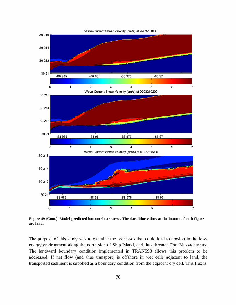
78

Figure 49 (Cont.). Model-predicted bottom shear stress. The dark blue values at the bottom of each figure are land.

The purpose of this study was to examine the processes that could lead to erosion in the low-energy environment along the north side of Ship Island, and thus threaten Fort Massachusetts. The landward boundary condition implemented in TRANS98 allows this problem to be addressed. If net flow (and thus transport) is offshore in wet cells adjacent to land, the transported sediment is supplied as a boundary condition from the adjacent dry cell. This flux is

79

Figure 50 (Cont.). Total Suspended Sediment calculated by TRANS98.

80

Figure 51. Seafloor elevation predicted by TRANS98

81

Figure 52. Cross-section of bed change and water depth along -88.96949 Longitude (~560m east of Fort Massachusetts).

Figure 53. Cross-section of seafloor elevation and water dept along column 140.

82

recorded as erosion from the coast. The fluxes at four times along Ship Island are plotted in Fig.

55. The x axis spans the length of the domain. Fort Massachusetts is located at -88.9722. Erosion is limited to the ends of the islands with slightly more predicted at the western end. The greatest erosion occurs early during the simulation, when currents were westward (Fig. 49, Top). Coastal erosion is almost 0.01 m3/m (100 cm3/m) of coast near the fort at 1200 on March 20. This doesn’t sound like much, but in the 10 cm water depths here this can account for ~10 cm of erosion per 3 min time step. Of course, we should use a more conservative water depth of 50 cm near the coast (see Fig. 54). For this depth, a cumulative erosion volume of ~0.5 m3/m (Fig. 56) would result in ~1 m of erosion during a single cold front. Since there are tens of cold fronts just like this one per winter, a conservative estimate for annual coastal retreat of 10 m is quite reasonable. This order of magnitude coastal erosion was not observed at Ship Island during the measurement period because of the passage of a tropical cyclone, which tends to restore sediment to the coast at this location (Fig. 46). There was measured sediment loss from offshore as suggested in the model predictions, however (Fig. 51). Of course, some of the sediment would be transported back to the beach during the summer by tides and weaker waves, or transported by the wind across the island from the open-water side.

Figure 54. Cross-section of seafloor elevation along column 80.

83

Figure 55. Coastal erosion at individual time steps along the north side of Ship Island.

84

Figure 56. Cumulative coastal erosion along the north side of Ship Island.

85

7 Summary

7.1 The nearshore environment

The four cases presented in this report span the breadth of problems encountered in the nearshore zone. They also demonstrate the difficulties inherent in studying this dynamic zone with observations and numerical models. The scales range from > 3 km to 5 m and from 1 hour to 3 minutes. These studies also help dispel the simplified concept of the nearshore zone being dominated by waves. This paradigm was developed from specific studies conducted on beaches like Duck, N. Carolina, and in wave tanks. These previous studies have been critical in understanding waves on beaches, but they are of less use in low-wave-energy environments like those discussed in this report.

The examples are presented in the chronological order in which they were undertaken. The first two, a powerful northeaster storm (the SandyDuck storm of October 1997) and Hurricane Isabel making landfall on the Outer Banks of N. Carolina, have been published (Keen, Beavers et al. 2003; Keen, Rowley et al. 2005). It was possible to reach a satisfactory conclusion with these two because of the relative simplicity of modeling the coastal transport system during storms. These severe storms are wave-dominated events and it is much easier to capture one or two oceanographic forces (e.g., storm waves and storm-surge currents) than overlapping processes with similar magnitudes, which was the case for the latter two examples, which demonstrate that the astronomical tides, wind-driven currents, coastal currents, wave-driven currents, baroclinic currents, storm waves, swell, and various substances within the water, all conspire to produce the signals that are observed by instruments in the nearshore environment. The Ship Island study was included in a proceedings volume (Keen, Stone et al. 2003) with the hydrodynamic modeling with POM and SWAN published in a separate paper (Keen 2002). The Santa Rosa Island beach study has only been presented orally (Keen, Stavn et al. 2006; Keen 2009).

The reason for the failure to close the last two studies is now obvious; it is the complex overlap of different processes and scales and the lack of adequate observations and appropriate numerical models. However, it is these more complex problems that are of greatest interest to the Navy because of the need for accurate predictions of nearshore properties that impact littoral operations in the surf zone. This requirement is the impetus for continuing efforts to understand the nearshore environment using observations and numerical models.

7.2 Observations

The examples discussed in this report exemplify the difficulty of acquiring comprehensive observations in nearshore studes. This is as much a problem of scale as instrument availability. The most successful modeling-measurement study presented here (Section 3) occurred on an

86

open beach during a severe storm. This is because of a long-term commitment by federal agencies (e.g., ACE, ONR, and USGS) to collecting observations at the FRF (http://www.frf.usace.army.mil/). This led to the development of special instrumentation that is suitable for a high-wave energy environment. These field programs required substantial planning and were sufficiently long to capture a range of flow conditions at Duck. The FRF is unsuitable for large-scale observations, however, because its overall purpose is to study wave-driven processes in the surf zone. A more expansive objective motivates the Nearshore Canyon Experiments near the U. Calif. at San Diego, which encompass a larger domain (see http://science.whoi.edu/users/elgar/NCEX/ncex.html).

The spatial scales represented by the Hurricane Isabel erosion study (Section 4) cannot be captured by typical coastal oceanographic observation systems (e.g., tide gauges and buoys). Hurricanes have occasionally been well sampled by opportunistic measurement systems, however, such as when Hurricane Andrew made landfall on the Louisiana coast in 1992 after crossing the LATEX moorings (Keen and Glenn 1998; Keen and Glenn 1999). These cases are rare and do not represent typical nearshore observations; furthermore, the nearshore data from H. Andrew were limited to tide gauges and C-MAN stations (Coastal-Marine Automated Network). The LATEX moorings were all located in water depths >15 m. Thus it is unlikely that useful observations of oceanographic processes during tropical cyclones will be available for the nearshore in the forseeable future, and we must improve the use of post-event analysis of geological and morphological effects like coastal erosion and storm bed deposition.

The results from Santa Rosa Island (Section 5) are presented in detail because this study reflects a concerted effort to characterize the hydrodynamic and optical nearshore environment as completely as possible. A full suite of data was collected at two locations but the observations do not resolve external forcing, which is indicated as a major factor during the field study. The observation scale of this experiment was similar to that of efforts at the FRF but with its primary interest being the optical environment. The low-energy environment did not require the investment in robust instrumentation required at Duck, however. Even with the limited spatial and temporal coverage of the data, it has been possible to validate both hydrodynamic and sedimentation/optical models and evaluate, at least qualitatively, the impact of external factors on the observations. Data sets such as those collected in August 1994 and March 1995 would be greatly improved with the inclusion of oceanographic observations from outside the immediate study area. This would permit more extensive analysis of external forcing.

Unlike the previous examples, the Ship Island study was originally motivated by a real problem that required a practical analysis of its causes so that an effective solution could be formulated (Chaney and Stone 1996). In this respect, this study is similar to what would be needed for naval applications; for example, determining the best location for the placement of JLOTS structures during amphibious operations. There is a significant difference, however, in that the

87

beach profiles were made over a year-long study in order to characterize erosion trends within the area. The limited hydrographic data collected at Fort Massachusetts could be supplemented by nearby buoys and tide stations in order to place the small-scale problem within the context of regional circulation. This compilation of data is represented by the use of existing validated flow data from POM for the area using conincidental (and fortuitous) measurements made by NRL in March of 1997 (Keen 2002). This fusion of different data sets will become more important in nearshore mulitdisciplinary studies of the future. It is also closer to the operational environment in which navy customers operate.

7.3 Models

These studies demonstrate three important principles in nearshore prediction: (1) the need for models that represent different physical processes, such as hydrodynamics, sedimentation, morphology, and optics; (2) individual models must be applicable to a range of space and time scales; and (3) it must be possible to substitute similar models (or observations) into a model system. These principles have been partly incorporated in efforts at NRL like MCEL (Model Coupling Environmental Library, http://www.nrl.navy.mil/content.php?P=04REVIEW167), ESMF (Earth System Modeling Framework, http://www.earthsystemmodeling.org/), and the relocatable NCOM system. For example, POM, SWAN, and LSOM were implemented in MCEL whereas ESMF incorporates NCOM and SWAN, and NCOM is included along with NCODA (Navy Coupled Ocean Data Assimilation) (Cummings 2005) in the relocatable system. Details of these modeling systems are beyond the scope of this report, however. The specific method used to couple or link the individual models has not been discussed in these examples because they focus on understanding hydrodynamic and sedimentation processes.

The most important conclusion of these studies has been the critical dependence of sedimentation on hydrodynamics. Nowhere is this more apparent than in determining the causes of unreasonably high levels of noise in the seafloor height at Fort Massachusetts (see Appendix A). This nonlinear dependence is deterministic and may be a major cause of variability in storm beds; however, this issue cannot be settled until sources of uncertainty are reduced. The correlation between hydrodynamic forcing and gradients in the bottom stress, which produce erosion and deposition through mass continuity, is the reason that large-scale problems (km’s and hours) produce realistic results whereas nearshore examples can easily become meaningless. This concept further applies to environments in which the forcing is limited to one or two factors, as with the SandyDuck storm.

Wave-driven flow has been incorporated using the SHORECIRC model in an effort to explore the sensitivity of nearshore sedimentation to hydrodynamics. The realistic results discussed in Sections 5 and 6 demonstrate the determinism of this model, but the relative magnitude of the flow is frequently low compared to external flows like the astronomical tide in these low-wave-

88

energy environments. A recent study by (Haas and Warner 2009) has demonstrated that realistic wave-driven flow can be incorporated in a primitive equation model like ROMS (Regional Ocean Modeling System) by using additional momentum terms.

These examples have shown the limitations of using primitive equation models like POM and NCOM for nearshore simulations. The major restriction on their use is the drying of grid cells as the water level for a cell decreases below its water depth. This is exemplified in the last two cases, which extrapolated steady currents to all water depths. It was also an issue in predicting breaching of Hatteras Island by Hurricane Isabel; the morphodynamic analysis presented in Section 4 was necessary because NCOM does not allow a change in the land mask and the associated abrupt changes in the model grid. The results show that a well-constructed model like NCOM can be used at a range of spatial scales as long as the basic assumptions (e.g., hydrostatic flow and no wetting/drying) are valid, however. The NCOM model was used to compute steady currents for the Isabel and Santa Rosa Island studies because it meets requirement (2), working well at different scales, somewhat better than POM.

An unresolved issue in simulating sedimentation processes is the degree to which hydrodynamics and sedimentation should be coupled. For example, sedimentation is computed as part of the main ROMS program. This approach has not been used in the cases discussed herein because of the continuing development of the TRANS98 model. Both the MCEL and ESMF modeling systems would permit both one-way and two-way coupling between models. The MCEL system has been used with TRANS98 but not as part of this study. ESMF does not currently incorporate a sedimentation module. The examples presented herein show that TRANS98 works at a range of scales similar to NCOM and SWAN, which is why these three models have been used together. SHORECIRC cannot be applied to larger scales and it has significant restrictions on open boundaries, which necessitates using it in a manner that allows independence with respect to grid selection. It is apparent from the tests discussed in Appendices A and B that there is feedback between sedimentation and hydrodynamics in very shallow water. In order to calculate stable, accurate solutions in these environments, therefore, it is necessary to couple these models.

The third principle follows from the need to achieve the greatest possible stability while calculating an accurate solution for nearshore processes. This requirement has motivated replacing the REFDIF wave model (http://chinacat.coastal.udel.edu/programs/refdif/refdif.html) with SWAN for wave-driven flows. It has also led to the replacement of WAM3 (Wave Model third genertion) by SWAN for regional simulations, and POM with NCOM for a range of problems. Within the MCEL system, this principle was applied to the simultaneous use of ADCIRC and POM working with TRANS98. The potential use of LSOM (updated TRANS98) and HQCM (HydroQual Contaminant Model) for coastal sedimentation computations will be discussed in a future report. Since the objective of these simulations is to predict sedimentation

89

processes, this flexibility can be a significant advantage for both scientific and operational problems.

7.4 Future work

The cases presented in this report show what can be done with existing models but they do not represent the state of the art in nearshore model systems. This is partly because of the different interests of stakeholders in the nearshore/estuarine environments. There are as nearly many nearshore modeling approaches as there are coastal engineers, but three systems have been developed that are readily available for these problems: (1) Delft3D (http://delftsoftware.wldelft.nl/index.php?option=com_frontpage&Itemid=57); (2) NearCoM (Nearshore Community Model, http://chinacat.coastal.udel.edu/programs/nearcom/index.html); and (3) the Regional Modeling System (ROMS: http://www.myroms.org/), which is applicable to a narrower suite of nearshore problems. Delft3D has been developed as a commercial modeling system and it is widely in use today for both nearshore and estuarine problems. A broad license has been purchased by ONR for navy applications.

The problem of bridging the different dynamic scales encountered in nearshore problems has been partially addressed through the use of a suite of nested models and/or grids. This approach has been used in three of these examples. The results show, however, that there are some problems that must be dealt with in this kind of approach. The known difficulty of generating spurious signals (noise) at boundaries between nests has led to a very conservative grid ratio of 3:1 being used for most applications. This limits how much external forcing can be propagated onto a nearshore grid; this problem occurred at Santa Rosa Island (see Section 5). The difficulties encountered at Ship Island when the coarse grid (~800 m) used for POM was interpolated to the fine grid (~5.5 m) suggest that this problem would be greatly exacerbated in supplying boundary conditions for a nonconservative tracer like suspended sediment. An alternative approach is the use of unstructured grids for nearshore problems (Utnes 1993), which avoid the use of boundaries between local and external regions. These models have proven highly effective in barotropic flows and they have been applied with some success to stratified conditions as well (Le Normant 2000). Both nesting and unstructured grids suffer from the same drawback, they cannot adapt as the spatial scales change. This is a very important factor in nearshore and estuarine regions where salinity, temperature, and turbulence respond to rapidly changing winds and input from terrestrial sources. This problem is being addressed by a new generation of adaptive grids, as represented by ICOM (Ford, Pain et al. 2004a; 2004b) and the Gnu Flow Solver, Gerris (Popinet 2003).

The final element required to predict ocean dynamics within nearshore and estuarine environments is the use of available observations and archived model results. It has been demonstrated that using observations to force sedimentation and optical models in coastal areas

90

produces much better prediction of sediments and thus optical properties (Keen and Stavn 2000). This approach is useful for validating a sedimentation model because it eliminates the uncertainty associated with currents from a hydrodynamic model that is itself imperfect. The SandyDuck study (Section 3) used measured currents to drive a sedimention model. Observed waves were used in both the SandyDuck and Santa Rosa Island studies because of their small model domains. Maximizing the use of available data in nearshore regions can be aided by the use of quality control and assimilation algorithms like those contained within NCODA (Cummings 2005), which can be used to merge or “fuse” data from different sensors and times to produce useful fields.

8 References

Bailard, J. A. (1982). "An energetic total load sediment transport model for a plane sloping beach." Ocean Science and Engineering 7(2): 229-277.

Bailard, J. A. and D. L. Inman (1981). "An Energetics Bedload Model for a Plane Sloping Beach - Local Transport." Journal of Geophysical Research-Oceans and Atmospheres 86(Nc3): 2035-2043.

Barron, C. N., L. F. Smedstad, et al. (2004). "Validation of the 1/8_ global Navy Coastal Ocean Model nowcast/forecast system,." Navigator Spring 2004: 5-8.

Beavers, R. L. (1999). Storm sedimentation in the surf zone and inner continental shelf, Duck, North Carolina. Geological Sciences. Chapel Hill, North Carolina, University of North Carolina. Ph.D.: 250.

Bowen, A. J. (1980). Simple models of nearshore sedimentation: Beach profiles and longshore bars. The Coastline of Canada. S. B. McCann, Geologic Survey of Canada. 80-11: 1-11.

Brocchini, M. and T. E. Baldock (2008). "Recent advances in modeling swash zone dynamics: Influence of surf-swash interaction on nearshore hydrodynamics and morphodynamics." Reviews of Geophysics 46(3): -.

Chaney, P. L. and G. W. Stone (1996). "Soundside erosion of a nourished beach and implications for winter cold front forcing: West Ship Island, Mississippi." Shore and Beach 64: 27-33.

Cobb, M., T. R. Keen, et al. (2008). "Modeling the circulation of the Atchafalaya Bay system during winter cold front events. Part 1: Model description and validation." Journal of Coastal Research 24(4): 1036-1047.

Cobb, M., T. R. Keen, et al. (2008). "Modeling the circulation of the Atchafalaya Bay system, part 2: River plume dynamics during cold fronts." Journal of Coastal Research 24(4): 1048-1062.

91

Cummings, J. A. (2005). "Operational multivariate ocean data assimilation." Quarterly Journal of the Royal Meteorological Society 131: 3583-3604.

Dally, W. R. and R. G. Dean (1984). "Suspended Sediment Transport and Beach Profile Evolution." Journal of Waterway Port Coastal and Ocean Engineering-Asce 110(1): 15-33.

Egbert, G. D., A. F. Bennett, et al. (1994). "Topex/Poseidon Tides Estimated Using a Global Inverse Model." Journal of Geophysical Research-Oceans 99(C12): 24821-24852.

Ford, R., C. C. Pain, et al. (2004). "A nonhydrostatic finite-element model for three-dimensional stratified oceanic flows. Part I: Model formulation." Monthly Weather Review 132(12): 2816-2831.

Ford, R., C. C. Pain, et al. (2004). "A nonhydrostatic finite-element model for three-dimensional stratified oceanic flows. Part II: Model validation." Monthly Weather Review 132(12): 2832-2844.

Fox, W. T. and R. A. Davis (1973). "Simulation Model for Storm Cycles and Beach Erosion on Lake-Michigan." Geological Society of America Bulletin 84(5): 1769-1790.

Friedman, G. M. and J. E. Sanders (1978). Principles of Sedimentology. New York, John Wiley.

Gallagher, E. L., S. Elgar, et al. (1998). "Observations of sand bar evolution on a natural beach." Journal of Geophysical Research-Oceans 103(C2): 3203-3215.

Glenn, S. M. and W. D. Grant (1987). "A Suspended Sediment Stratification Correction for Combined Wave and Current Flows." Journal of Geophysical Research-Oceans 92(C8): 8244-8264.

Gould, R. W. and R. A. Arnone (1997). "Remote sensing estimates of inherent optical properties in a coastal environment." Remote Sensing of Environment 61(2): 290-301.

Gould, R. W. and R. A. Arnone (1998). "Three-dimensional modelling of inherent optical properties in a coastal environment: coupling ocean colour imagery and in situ measurements." International Journal of Remote Sensing 19(11): 2141-2159.

Haas, K., I. A. Svendsen, et al. (1998). Numerical modeling of nearshore circulation on a barred beach with rip channels. 26th International Conference on Coastal Engineering, American Society of Civil Engineers: 801-814.

Haas, K. A. and J. C. Warner (2009). "Comparing a quasi-3D to a full 3D nearshore circulation model: SHORECIRC and ROMS." Ocean Modelling 26(1-2): 91-103.

Hanson, H. and N. C. Kraus (1991). "Numerical-Simulation of Shoreline Change at Lorain, Ohio." Journal of Waterway Port Coastal and Ocean Engineering-Asce 117(1): 1-18.

92

Hequette, A. and P. R. Hill (1995). "Response of the Seabed to Storm-Generated Combined Flows on a Sandy Arctic Shoreface, Canadian-Beaufort Sea." Journal of Sedimentary Research Section a-Sedimentary Petrology and Processes 65(3): 461-471.

Holland, G. J. (1980). "An Analytic Model of the Wind and Pressure Profiles in Hurricanes." Monthly Weather Review 108(8): 1212-1218.

Holman, R. A. and A. J. Bowen (1982). "Bars, Bumps, and Holes - Models for the Generation of Complex Beach Topography." Journal of Geophysical Research-Oceans and Atmospheres 87(Nc1): 457-468.

Holman, R. A. and A. H. Sallenger (1993). "Sand bar generation: A discussion of the Duck experiment series." Journal of Coastal Research Special Issue No. 15: 76-92.

Howd, P. A., A. J. Bowen, et al. (1992). "Edge Waves in the Presence of Strong Longshore Currents." Journal of Geophysical Research-Oceans 97(C7): 11357-11371.

Hsu, Y. L., W. E. Richards, et al. (2000). Application of SWAN in the Mississippi Sound. Sixth International Workshop on Wave Hindcasting and Forecasting. Monterey, California, Meteorological Service of Canada: 398-403.

Kara, A. B., C. N. Barron, et al. (2006). "Validation of interannual simulations from the 1/8 degrees global Navy Coastal Ocean Model (NCOM)." Ocean Modelling 11(3-4): 376-398.

Keeley, J. R. (1977). "Nearshore Currents and Beach Topography, Martinique Beach, Nova-Scotia." Canadian Journal of Earth Sciences 14(8): 1906-1915.

Keen, T. R. (2002). "Waves and currents during a winter cold front in the Mississippi bight, Gulf of Mexico: Implications for barrier island erosion." Journal of Coastal Research 18(4): 622-636.

Keen, T. R. (2009). Problems in simulating nearshore dynamics with numerical models. Invited Seminar. New York, City College of New york.

Keen, T. R., R. L. Beavers, et al. (2003). "Shoreface sedimentation during a northeaster at Duck, North Carolina, U.S.A." Journal of Coastal Research 19(1): 24-40.

Keen, T. R. and M. Byrd (2006). Simulating Salinity Constraints on the Spread of Microcystis Aeruginosa in San Francisco Bay using a Numerical Hydrodynamic Model.

Keen, T. R. and Y. Furukawa (2007). A modular entrainment model for cohesive sediment. Estuarine and Coastal Fine Sediment Dynamics. J. P. Y. Maa. Gloucester Point, Virginia, Elsevier: 184-202.

Keen, T. R., Y. Furukawa, et al. (2006). "Geological and oceanographic perspectives on event bed formation during Hurricane Katrina." Geophysical Research Letters 33(23): -.

93

Keen, T. R. and S. M. Glenn (1994). "A Coupled Hydrodynamic Bottom Boundary-Layer Model of Ekman Flow on Stratified Continental Shelves." Journal of Physical Oceanography 24(8): 1732-1749.

Keen, T. R. and S. M. Glenn (1998). "Factors influencing model skill for hindcasting shallow water currents during Hurricane Andrew." Journal of Atmospheric and Oceanic Technology 15(1): 221-236.

Keen, T. R. and S. M. Glenn (1999). "Shallow water currents during hurricane Andrew." Journal of Geophysical Research-Oceans 104(C10): 23443-23458.

Keen, T. R. and F. Harding (2008). "Seasonal patterns of exchange between St. Louis Bay and Mississippi Sound, U.S.A." Eos, Transactions of the American Geophysical Union(Ocean Sciences Meeting, Orlando, Florida): OS-262.

Keen, T. R., D. S. Ko, et al. (2006). "Potential transport pathways of terrigenous material in the Gulf of Papua." Geophysical Research Letters 33(4): -.

Keen, T. R. and S. J. Murphy (1999). Developing a relocatable coastal ocean forecast model. Oceanology '99, Singapore.

Keen, T. R., C. Rowley, et al. (2005). Oceanographic factors and erosion of the outer banks during Hurricane Isabel. Hurricane Isabel in Perspective. K. G. Sellner, Chesapeake Research Consortium. CRC Publication 05-160: 65-72.

Keen, T. R. and R. L. Slingerland (1993). "A Numerical Study of Sediment Transport and Event Bed Genesis during Tropical Storm Delia." Journal of Geophysical Research-Oceans 98(C3): 4775-4791.

Keen, T. R., R. L. Slingerland, et al. (2010). Sediment transport on continental shelves: Storm bed formation and preservation in heterogeneous sediments. Fukuoka, Japan, International Association of Sedimentologists. Special Publication: in press.

Keen, T. R. and R. H. Stavn (2000). Developing a capability to forecast coastal ocean optics: minerogenic scattering. 6th International Conference on Estuarine and Coastal Modeling, American Society of Civil Engineers: 178-193.

Keen, T. R., R. H. Stavn, et al. (2006). "Predicting the effects of physical and optical processes on Lidar performance at Hamlet’s Cove, Florida." Eos, Transactions of the American Geophysical Union 87(36): OS26N-12.

Keen, T. R., G. W. Stone, et al. (2003). Barrier island erosion during a winter cold front in Mississippi Sound. Coastal Sediments 2003, Clearwater Beach, Florida, American Society of Civil Engineers.

94

Kim, S. C., L. D. Wright, et al. (1997). "The combined effects of synoptic-scale and local-scale meteorological events on bed stress and sediment transport on the inner shelf of the Middle Atlantic Bight." Continental Shelf Research 17(4): 407-433.

Ko, D. S., R. H. Preller, et al. (2003). "Transport reversals at Taiwan strait during October and November 1999." Journal of Geophysical Research-Oceans 108(C11): -.

Komar, P. D. (1971). "Mechanics of Sand Transport on Beaches." Journal of Geophysical Research 76(3): 713-&.

Lawrence, P. L. and R. G. D. DavidsonArnott (1997). "Alongshore wave energy and sediment transport on southeastern Lake Huron, Ontario, Canada." Journal of Coastal Research 13(4): 1004-1015.

Le Normant, C. (2000). "Three-dimensional modelling of cohesive sediment transport in the Loire estuary." Hydrological Processes 14(13): 2231-2243.

Lee, C., D. J. Schwab, et al. (2007). "Numerical modeling of mixed sediment resuspension, transport, and deposition during the March 1998 episodic events in southern Lake Michigan." Journal of Geophysical Research-Oceans 112(C2): -.

Leuttich, R. A., J. J. Westerink, et al. (1992). ADCIRC: An advanced three-dimensional circulation model for shelves, coasts, and estuaries. Report 1: Theory and methodology of ADCIRC-2DDI and ADCIRC-3DI. Technical Report: 168.

Martin, P. J., S. R. Smith, et al. (2009). Use of the Oregon State University Tidal Inversion Software (OTIS) to generate improved tidal prediction in the East-Asian seas. Memorandum Report, Naval Research Laboratory: 29.

Nicholls, R. J., W. A. Birkemeier, et al. (1998). "Evaluation of depth of closure using data from Duck, NC, USA." Marine Geology 148(3-4): 179-201.

Pierce, J. W. (1969). "Sediment Budget Along a Barrier Island Chain." Sedimentary Geology 3(1): 5-&.

Plant, N. G., B. G. Ruessink, et al. (2001). "Morphologic properties derived from a simple cross-shore sediment transport model." Journal of Geophysical Research-Oceans 106(C1): 945-958.

Popinet, S. (2003). "Gerris: a tree-based adaptive solver for the incompressible Euler equations in complex geometries." Journal of Computational Physics 190(2): 572-600.

Rakha, K. A. (1998). "A Quasi-3D phase-resolving hydrodynamic and sediment transport model." Coastal Engineering 34(3-4): 277-311.

95

Roberts, H. H., O. K. Huh, et al. (1987). Impact of cold-front passages on geomorphic evolution and sediment dynamics of the complex Louisiana coast. Coastal Sediments 1987. New Orleans, Louisiana, American Society of Civil Engineers: 1950-1963.

Robertson, W., K. Q. Zhang, et al. (2007). "Hurricane-induced beach change derived from airborne laser measurements near Panama City, Florida." Marine Geology 237(3-4): 191-205.

Roelvink, J. A. and I. Broker (1993). "Cross-Shore Profile Models." Coastal Engineering 21(1-3): 163-191.

Rogers, W. E., P. A. Hwang, et al. (2003). "Investigation of wave growth and decay in the SWAN model: Three regional-scale applications." Journal of Physical Oceanography 33(2): 366-389.

Rosen, P. S. (1978). "Regional Test of Bruun Rule on Shoreline Erosion." Marine Geology 26(1-2): M7-M16.

Ruessink, B. G., K. T. Houwman, et al. (1998). "The systematic contribution of transporting mechanisms to the cross-shore sediment transport in water depths of 3 to 9 m." Marine Geology 152(4): 295-324.

Ruggiero, P., P. D. Komar, et al. (2001). "Wave runup, extreme water levels and the erosion of properties backing beaches." Journal of Coastal Research 17(2): 407-419.

Sanchez-Arcilla, A., J. A. Jimenez, et al. (2001). Sensitivity analysis of longshore sediment transport rate estimations in a higly eroding coast, the Montroig Beach (Terragona, Spain). Coastal Dynamics 2001. H. Hanson and M. Larson, American Society of Civil Engineers: 112-121.

Schoonees, J. S. and A. K. Theron (1995). "Evaluation of 10 Cross-Shore Sediment Transport Morphological Models." Coastal Engineering 25(1-2): 1-41.

Slingerland, R., R. W. Selover, et al. (2008). "Building the Holocene clinothem in the Gulf of Papua: An ocean circulation study." Journal of Geophysical Research-Earth Surface 113(F1): -.

Srinivas, R. and R. G. Dean (1996). "Cross-shore hydrodynamics and profile response modeling." Coastal Engineering 27(3-4): 195-221.

Stapor, F. W. (1971). "Sediment Budgets on a Compartmented Low-to-Moderate Energy Coast in Northwest Florida." Marine Geology 10(2): M1-&.

Stavn, R. H. and T. R. Keen (2004). "Suspended minerogenic particle distributions in high-energy coastal environments: Optical implications." Journal of Geophysical Research-Oceans 109(C5): -.

96

Stone, G. W. (1998). Beach nourishment monitoring program at Fort Massachusetts, West Ship Island, Mississippi, National Park Service. I: 16.

Stone, G. W. and F. W. Stapor (1996). "A nearshore sediment transport model for the northeast Gulf of Mexico coast, USA." Journal of Coastal Research 12(3): 786-793.

Stone, G. W., F. W. Stapor, et al. (1992). "Multiple Sediment Sources and a Cellular, Non-Integrated, Longshore-Drift System - Northwest Florida and Southeast Alabama Coast, USA." Marine Geology 105(1-4): 141-154.

Stone, G. W. and P. Wang (1999). The importance of cyclogenesis on the short-term evolution of Gulf coast barriers. Transactions, Gulf Coast Association of Geological Societies.

Styles, R. B. (1998). A continental shelf bottom boundary layer model: Development, calibration and application to sediment transport in the Middle Atlantic Bight. Institute of Marine and Coastal Sciences. New Brunswick, Rutgers University. Ph.D.: 261.

Swift, D. J. P., A. W. Niedorida, et al. (1985). "Barrier island evolution, Middle Atlantic shelf, U. S. A. Part I: Shoreface dynamics." Marine Geology 63: 331-361.

Tamigineaux, E., L. Legendre, et al. (1999). "Seasonal Dynamics and Potential Fate of Size-fractionated Phytoplankton in a Temperate Nearshore Environment (Western Gulf of St Lawrence, Canada)." Estuarine, Coastal and Shelf Science 48(2): 253-269.

Thieler, E. R., O. H. Pilkey, et al. (2000). "The use of mathematical models to predict beach behavior for US coastal engineering: A critical review." Journal of Coastal Research 16(1): 48-70.

Thornton, E. B., R. T. Humiston, et al. (1996). "Bar/trough generation on a natural beach." Journal of Geophysical Research-Oceans 101(C5): 12097-12110.

Trembanis, A. C., O. H. Pilkey, et al. (1999). "Comparison of beach nourishment along the US Atlantic, Great Lakes, Gulf of Mexico, and New England shorelines." Coastal Management 27(4): 329-340.

Utnes, T. (1993). "Finite-Element Current and Sediment Transport Modeling." Continental Shelf Research 13(8-9): 891-902.

Valverde, H. R., A. C. Trembanis, et al. (1999). "Summary of beach nourishment episodes on the US East Coast barrier islands." Journal of Coastal Research 15(4): 1100-1118.

Walker, N. D. and A. B. Hammack (2000). "Impacts of winter storms on circulation and sediment transport: Atchafalaya-Vermilion Bay region, Louisiana, USA." Journal of Coastal Research 16(4): 996-1010.

97

Weidemann, A. D., R. H. Stavn, et al. (1995). "Error in Predicting Hydrosol Backscattering from Remotely-Sensed Reflectance." Journal of Geophysical Research-Oceans 100(C7): 13163-13177.

Wright, L. D., J. D. Boon, et al. (1986). "Response of the Mid Shoreface of the Southern Mid-Atlantic Bight to a Northeaster." Geo-Marine Letters 6(3): 153-160.

Wright, L. D., J. D. Boon, et al. (1991). "Modes of Cross-Shore Sediment Transport on the Shoreface of the Middle Atlantic Bight." Marine Geology 96(1-2): 19-51.

Wright, L. D. and A. D. Short (1984). "Morphodynamic Variability of Surf Zones and Beaches - a Synthesis." Marine Geology 56(1-4): 93-118.

Wright, L. D., A. D. Short, et al. (1985). "Short-Term Changes in the Morphodynamic States of Beaches and Surf Zones - an Empirical Predictive Model." Marine Geology 62(3-4): 339-364.

Wright, L. D., J. P. Xu, et al. (1994). "Across-Shelf Benthic Transports on the Inner Shelf of the Middle Atlantic Bight during the Halloween Storm of 1991." Marine Geology 118(1-2): 61-77.

Xu, J. P. and L. D. Wright (1998). "Observations of wind-generated shoreface currents off duck, north Carolina." Journal of Coastal Research 14(2): 610-619.

98

Appendix A: Notes on TRANS98 Computations for Bottom Properties.

A1 General problem

A problem was encountered in the Ship Island erosion study. The computed bed properties were irregular for no obvious reason. This can be expanded to mean that all plotted variables begin to show the impact of some unknown process (es), possibly numerical, that appear (s) in u* and is (are) especially pronounced in the erosion depth. This problem appears to be associated with calculating transport (Fig. A1). It appears that there is a feedback loop operating, in which one of the model parameters becomes unstable and subsequently affects all others. The calculation loop for trans98 is shown in Figure A2. This will be referred to below.

The first calculation is for u* in subroutine NBM96, which suggests that it should be stable when the other variables are bad. A sequence of snapshots (Fig. A3) demonstrates this. There appears to be some irregularity even at the beginning of the run. We can compare the initial u* field to that from Figure A4 for the run with no transport. We see that they are the same. This implies that it is not the setup for transport that is causing the problem but the actual computations. Furthermore, the final time field (lower panel in Figure A4) reveals a smoothly varying field for u*, which is in stark contrast to the final field in Figure A3.

The default size distribution (Fig. A5) spans 2 to 330 microns (10-6 m), which introduces some excessive fine material but only very small quantities of it, as indicated by the low available weight percent (AWP) values in Figure A5. The median grain size is ~50 microns. The solution algorithm (Fig. A2) initially calculates the shear stress by first calculating the bed roughness (not shown), which is a function of ripple height, before finding the iterative solution for the bottom boundary layer (bbl) profile of currents and resulting shear stress. The model output is the final solution. We will examine this more closely using a reduced domain, which aids in analyzing the model fields.

A2 Ripple calculations

The ripple geometry is calculated from a series of lab and field experiments, which were used to parameterize the observed bed forms that occurred under different environmental conditions.

Ultimately, the ripple height and wavelength are found from sediment entrainment properties and existing conditions at the bed.

The model uses successive guesses for the ratio of the steady near-bottom current ur and the oscillatory current uw. The algorithm in TRANS98 solves for dimensionless variables using the unknown wave orbital diameter at the bed Ab. These dimensionless parameters allow the large amount of data to be simplified as in the Shields diagram (Fig. A6). These data suggest that

99

sediment entrainment is dependent on the maximum Shields parameter m, the critical Shields

parameter c, and the break-off shields parameter b.

The maximum Shields parameter for a given value of ua/ub (estimate of ur/uw) is given by:

m = fcw × [1 + (ua/ub) 2] / {2 × [( (-1) × g ×d )0.5 / uw] 2} (1)

where: fcw = wave-current friction factor (parameterized from laboratory experiments); ua/ub =

current guess for the ratio of the steady current ur to the wave current uw; = specific gravity of sediment mineral; g = gravity constant; and d = grain diameter. The friction factor fcw is dependent on the current value of ua/ub and an equation for the integrated friction over a wave cycle using Bessel functions. It is possible that it could produce discontinuities in bottom friction because the solution involves both +/- values, which must be corrected based on ua/ub. The value of ua/ub is modified after integration based on an error evaluation. If the solution does not converge, ad hoc measures are taken to assure a reasonable solution is found; this could lead to potential discontinuities in the result. The other parameters in (1) are either constant or smoothly changing. For example, uw is a function of the wave height and water depth. It is also possible that some of the parameterizations used in the model are inaccurate for smaller sizes.

The critical Shields parameter c is given by:

c = fc × A × (S*)B (2)

where: fc = a correction factor (a constant value of 1 is used in TRANS98); S* = dimensionless sediment parameter; A = constant > 0; and B = constant < 0. The value of A decreases as S* increases whereas B increases (less negative). The dimensionless sediment parameter S* is different for each sediment grain size; it is given by:

S* = d/(4 ) × ( (-1) × g ×d )0.5 (3)

where = kinematic viscosity (/). Note that the boundary Reynolds number Re* in Figure A6

(u*d/) is equivalent to d/o where o = thickness of the laminar sub-layer. Thus, o = /u*, which makes sense in that the balance between viscosity and shear stress will determine the behavior of both sediment particles and fluid near the bed.

The ratio m/c represents by how much the bottom shear forces exceed the sediment mobility

properties. There is a minimum value of c for each sediment size/density class incorporated in the Shields diagram. This minimum value is termed the break-off Shields parameter. It can be found from Figure A6 for any grain but it is useful to rewrite it in the same terms as the maximum Shields parameter discussed above. After manipulation (see Glenn and Grant, 1987),

the ratio of b/ c has been determined to equal 1.8×(S*)0.6 where the constants are based on

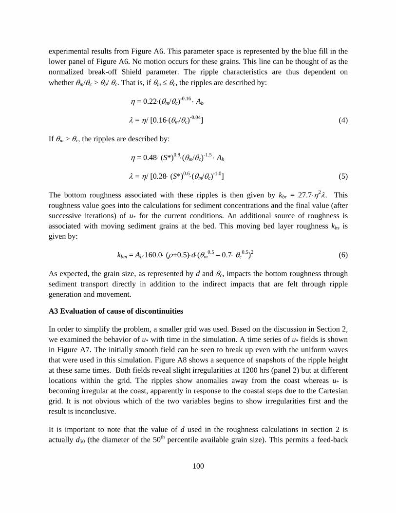
100

experimental results from Figure A6. This parameter space is represented by the blue fill in the lower panel of Figure A6. No motion occurs for these grains. This line can be thought of as the normalized break-off Shield parameter. The ripple characteristics are thus dependent on

whether m/c > b/ c. That is, if m c, the ripples are described by:

= 0.22(m/c)-0.16 Ab

= / [0.16(m/c)-0.04] (4)

If m > c, the ripples are described by:

= 0.48 (S*)0.8(m/c)-1.5 Ab

= / [0.28 (S*)0.6(m/c)-1.0] (5)

The bottom roughness associated with these ripples is then given by kbr = 27.72. This roughness value goes into the calculations for sediment concentrations and the final value (after successive iterations) of u* for the current conditions. An additional source of roughness is associated with moving sediment grains at the bed. This moving bed layer roughness kbs is given by:

kbm = Ab160.0 (+0.5)d(m0.5 – 0.7 c

0.5)2 (6)

As expected, the grain size, as represented by d and c, impacts the bottom roughness through sediment transport directly in addition to the indirect impacts that are felt through ripple generation and movement.

A3 Evaluation of cause of discontinuities

In order to simplify the problem, a smaller grid was used. Based on the discussion in Section 2, we examined the behavior of u* with time in the simulation. A time series of u* fields is shown in Figure A7. The initially smooth field can be seen to break up even with the uniform waves that were used in this simulation. Figure A8 shows a sequence of snapshots of the ripple height at these same times. Both fields reveal slight irregularities at 1200 hrs (panel 2) but at different locations within the grid. The ripples show anomalies away from the coast whereas u* is becoming irregular at the coast, apparently in response to the coastal steps due to the Cartesian grid. It is not obvious which of the two variables begins to show irregularities first and the result is inconclusive.

It is important to note that the value of d used in the roughness calculations in section 2 is actually d50 (the diameter of the 50th percentile available grain size). This permits a feed-back

101

between transport, which will preferentially move finer sizes, and the new ripple field associated with the deposited fine sediment. This will produce a smaller d50 where the sediment was deposited. This should in general produce smaller ripples and thereby less roughness; however, this is not necessarily the case because of the nonlinearities implied by the Shields diagram (Fig. A6). This was investigated by using a constant value for the bottom roughness, kb. The results are shown in Figure A9. The entrainment of sediment near the coast is seen in the much thicker suspended bed there, but the d50 for transported sediment shows ~60 micron (very fine sand) deposited at the offshore edge of the platform. This is slightly coarser than the d50 particles, which are 50 microns (see Fig. A5). There are also areas of coarser sand transport mid-way across the platform The most interesting result, however, is the similarity of the erosion depth pattern to that from Figure A1. Since this simulation did not have variable ripples because a constant (user input) value of kb makes the computation of ripples unnecessary.

It doesn't appear that the irregularities in the ripple field are responsible for the erosion depth but the pattern seen in Figure A8 clearly indicates that there is an underlying process responsible. The currents from POM were interpolated from a much larger grid, which can introduce an underlying pattern in the flow field. The diffusion and advection terms were turned off and only bed load was used to transport sediment in the next simulation. A comparison of the x-directed results for suspension, bed load, and diffusion only (Fig. A10) reveals an interesting pattern in the transport rates. All three modes of transport are dependent on the current field. Specifically, however, the diffusion rate is computed from the Smagorinsky algorithm (using FORTRAN pseudo-code):

DO I, J....

AHUV(I,J) = AHCON*DX*DY * SQRT( ((UB(I,J)-UB(I-1,J))/DX)**2

+((VB(I,J)-VB(I,J-1))/DY)**2

+.5E0*(.25*(UB(I-1,J+1)+UB(I,J+1)-UB(I-1,J-1)-UB(I,J-1))/DY

+.25*(VB(I+1,J-1)+VB(I+1,J)-VB(I-1,J-1)-VB(I-1,J))/DX)**2) (7)

ENDDO

Note that (7) is formulated in terms of the x and y components of velocity (UB, VB) being offset by +1/2 a grid cell (i.e., i+1/2, j+1/2). Equation (7) indicates the dependence of horizontal mixing on the gradient of the velocity field. The results in Figure A10 thus implicate the interpolation scheme in creating artificial gradients between the larger cells used by POM. These weak gradients could be sufficient to generate sporadic noise because of the sensitivity of transport to these gradients.

102

This potential source of trouble has been investigated by smoothing the input currents from POM using a built-in MATLAB® function, "smooth3." The improvement in the field can be examined using the x-axis diffusion terms for varying degrees of smoothing (Fig. A11). The bed load and suspended load transport components display similar patterns to the unsmoothed input simulation (Fig. A10) but the diffusion component (right panel) shows an irregular pattern that suggests that the error due to the interpolation from the coarser grid is decreased. It is also noteworthy that the suspended load maxima near the coast (center panel) are greatly reduced. The erosion depth is the primary result being examined now, so it is useful to see the impact on this variable of smoothing the input current field from POM. The erosion depth (Fig. A12) does not decrease or lose the lineation observed in Figure A1. For extensive smoothing, the area does become broader and new alongshore bands of increased erosion have appeared. This broadening of the erosion band results from the wider area of increased gradients in the transport flux. The bedload fluxes (Figs. A10 and A11) in fact show a divergence along this line, with westward transport to the west and eastward to the east.

This N-S line along the middle of the domain suggests that this is a zone of divergence in the flow that cannot be removed by smoothing. This result is significant for two reasons: (1) where such divergences occur, the model will predict systematic erosion that, once initiated, will be reinforced by subsequent processes associated with the newly deposited finer sediment; and (2) such a divergence can be caused by a process (e.g. wave-driven bed load) that is opposed to other processes (e.g., current driven suspended load). The final outcome will result from the interaction of these processes while being initiated by the weaker of the two (bed load tends to be weaker than suspended load). One result that was observed in these simulations along an E-W line (row=43) was the correlation between high erosion depth and small u*, ripples, and d50.

The over-riding consideration appears to be the mass flux computed by subroutine EROSION after all of the transport fluxes have been calculated. Smoothing the current fields and limiting resuspension and instantaneous erosion to the active layer depth helps control the fluxes but nothing can be done about the net flux at a cell. Previous versions of TRANS98 have attempted to limit this problem but they proved unsatisfactory overall. The current viewpoint is that the best that can be attained is to limit resuspension to the active layer and try and control erosion/deposition fluxes between the bed and the water column using the time step. Generally,

smaller time steps will reduce the size of the mass flux M of size class n through the t term in the seabed conservation equation:

Mn = t(Sn +Bn + Dn) (8)

where: Sn = gradient in suspended load; Bn = gradient in bed load; and Dn = gradient in horizontal mixing. For many of the previous applications of the model, reasonable results have been achieved using a time step of 1 hour. This may be too long for the very small grid used in

103

this study, however. For example, the weak currents (< 20 cm/s) measured at Fort Massachusetts would transport sediment by repeated resuspension ~720 m in 1 hour. This is the scale of model we have used for shelf applications. The grid at Ship Island is ~ 5 m, which suggests a time step of ~ 30 seconds is required to prevent cell jumping in a phenomenon often

referred to as "2x" noise, which suggests that the advection is exceeding the cell size and being resolved into split solutions as has been noticed in hydrodynamic modeling studies.

This problem was investigated using simulations for the Fort Massachusetts area with a time step of 30 s. These simulations produced a similar pattern of erosion oriented perpendicular to

the coast but the “2x” noise is significantly reduced for the first few time steps; however, by 6 hours, the pattern is appearing. Part of the reason for this can be seen in the change in bed d50 over time (Fig. A13). The initial erosion along a line perpendicular to the coast can be seen as early as 1 hr into the simulation (left panel). Finer material has been preferentially winnowed from the bed and transported to the west, leaving a coarser lag deposit behind and producing a fine layer where deposited. This pattern is then reinforced because the finer material produces smaller ripples and lower bed shear stresses. This process reinforces the initial transport pattern as seen in the larger ripples approaching shore in Figure A8. By hour 9 (right panel in Fig. A13), the bottom sediment grain size has become bimodal and shows a distinct pattern suggesting numerical causes rather than physical. The specific changes in AWP for representative size classes further demonstrate the nature of the problem. For example, both the 50 and 229 micron classes have initial AWP values of 5%. The 50 micron class (Fig. A14) is depleted in the bed at the coast (dark purple fill color) and along the across-shore lineation but it is widely deposited after 6 hours, with a few maxima. The 229 micron class is not as depleted offshore but is missing near the coast. The interesting result in this figure is that both of these size classes have been concentrated in a few maxima with broad areas of depletion in the bed, presumably by different processes, given their different critical shear stresses (see Fig. A5).

A4 Validation and testing of the modified TRANS98 (version 3.3) model.

It appears probable that there are several issues contributing to the results presented thus far in this report. To address these potential problems rigorously, a series of test cases were designed that would allow the physical and numerical parameterizations in the model to be examined independently. The test conditions and results are presented and summarized in Appendix B (TRANS98 Version 3 Evaluation). The problem has been greatly simplified in the UF and BF series of simulations by using one sediment size in the bed with a diameter of 73 microns.

The UF series of experiments (Table B1) demonstrate the correct implementation of the boundary conditions for open sea, land with no fluxes, and land with a sediment flux to seaward (Table B2). These results did require some modification of the model to correct errors that would have impacted the results noted above. The previous experiments indicate the difficulty

104

in discerning physical versus numerical causes of the irregularities in the bed properties. The first series of experiments discussed next, therefore, used only one size class, which required significant alterations of the model. During these modifications, several algorithms were changed as required.

The beach face experiments (BF... in Table B1) were designed to test the model algorithm for deposition/erosion when currents are onshore/offshore. The depositional regime (BF001) produced smooth results when a landward boundary condition was added that allowed cells to become land and thus outside the computational regime. Variations in wave height across the shoreface (N to S) were imposed by a depth-limited breaking criterion (HS < 0.7D), which does not allow excessive shear stresses in very shallow water (< 1m). Because of the low transport at the coast, the model predicts deposition just seaward, with only 1 row being lost to landward accretion. The net result is deposition of a platform at the coast (lower panel in Fig. A15).

The example of offshore currents and no erosion from the coast is explored in test BF002. Because of the very shallow water at the coast (10 cm), erosion exceeds 25 cm near the coast (upper panel in Fig. A16). The erosion does not occur at the coast because of the depth-limited wave heights and consequent low transport rates for depths < 50 cm. A small mound is deposited at 400 m after initial erosion has lowered the bed

Simulation BF003 is intended to reproduce a more realistic scenario with landward erosion of material to replace that lost to sea by offshore flow. The boundary conditions were modified to permit separate selection of type (land/open/closed) for the N, S, E, and W sides. This test included increasing currents seaward and resulting erosion of the shore face (Fig. A17) with less overall erosion than for the closed landward boundary of BF002, especially at the coast. Run BF004 was the symmetrical twin of BF003, which was intended to test the boundary condition for i-1/2 (j-1/2) cell faces on the W (S) boundaries. The bed elevation (Fig. A18) is the mirror image of BF003.

The model at this time appears to be numerically sound and stable for the kinds of conditions tested above. This formulation will be tested with a realistic case at Ship Island. Before proceeding to this test, we will evaluate the result of a smaller time step, 60 s. This test (BF005) produced bed elevations (Fig. A19) identical to BF004. The example from Ship Island (FM001) demonstrates similar responses to those predicted in the beach face simulations, with some extra complexities cause by the realistic bathymetry and forcing. The effect of the changes made to the code can be seen by comparing Figure A20 (after modification) to Figure A12, which shows the erosion depths for several size classes and less smoothing of the input currents. Note that deposition along the coast is much smoother. The final test in this series is FM003 (see Appendix B), which is the full Ship Island grid (424×200 cells) with smoothed forcing and one grain size. The solution (Fig. A21) can be compared to the initial solution in

105

this report (Fig. A1, second panel), which displayed the noise that prompted this study. The solution instead resembles the lower panel in Figure A1, which did not incorporate advection. The differences occur near Fort Massachusetts (circle in figures), where coastal erosion was greatest.

106

Figure A1. The top panel shows the problem of irregular erosion depth at Ship Island. The middle panel shows the u* field at the same time. The lower panel shows the u* field at the same time but when no transport was calculated. Note the smoothness of the resuspension simulation and the overall lower values near the island.

107

Program flow:

c

c I. Set up model grid and sediment distribution (SETUP).

c II. Do for all time steps:

c A. Calculate WHOI date (NEW_DATE).

c B. Model Input.

c 1. Read in waves and calculate bottom orbital

c parameters (AIRY).

c 2. Read in currents (CURRENTS).

c

c --------------------Start of BBLM block---------------

c

c C. Calculate combined wave-current bottom boundary layer (BBLM):

c 1. Find shear stress (NBM96).

c 2. Compute current and suspended sediment profiles

c (PROFILE2).

c 3. Calculate active layer thickness (BBLM).

c 4. For each sediment size class (BBLM):

c a. Compute resuspension depth.

c b. Adjust sediment profiles to reduce

c resuspension depth to active layer thickness

108

c (SPR1D).

c D. Calculate resuspension and reworking depths.

c E. Print bottom boundary layer variables (PNBM96).

c

c --------------------Start of transport block---------------

c

c F. Do for each size class of sediment:

c 1. Calculate bed load transport rate (BEDLOAD).

c 2. Suspended sediment transport rate (SUSP_LOAD).

c 3. Diffusion terms (DIFFUSION).

c 4. Solve sediment continuity equation (EROSION).

c a. Calculate erosion and deposition.

c b. Adjust suspended load transport rates to

c reduce erosion to active layer thickness

c (REDUCTION).

c 5. Sum coastal erosion for all size classes.

c G. Calculate sediment distribution within active layer

c (ACTIVE_LAYER).

c H. Compute transport and combined beds for current time step

c (BEDS).

c I. Calculate total (integrated size/depth) sediment transport

c rates (TOTAL_LOAD).

109

c J. Sum cumulative coastal erosion.

c K. Print bottom boundary layer variables (PTRN98).

c

c --------------------End of transport block---------------

c

c L. Print profiles and time series (MOORING).

c

c --------------------End of BBLM block---------------

c

Figure A2. Solution algorithm for trans98.

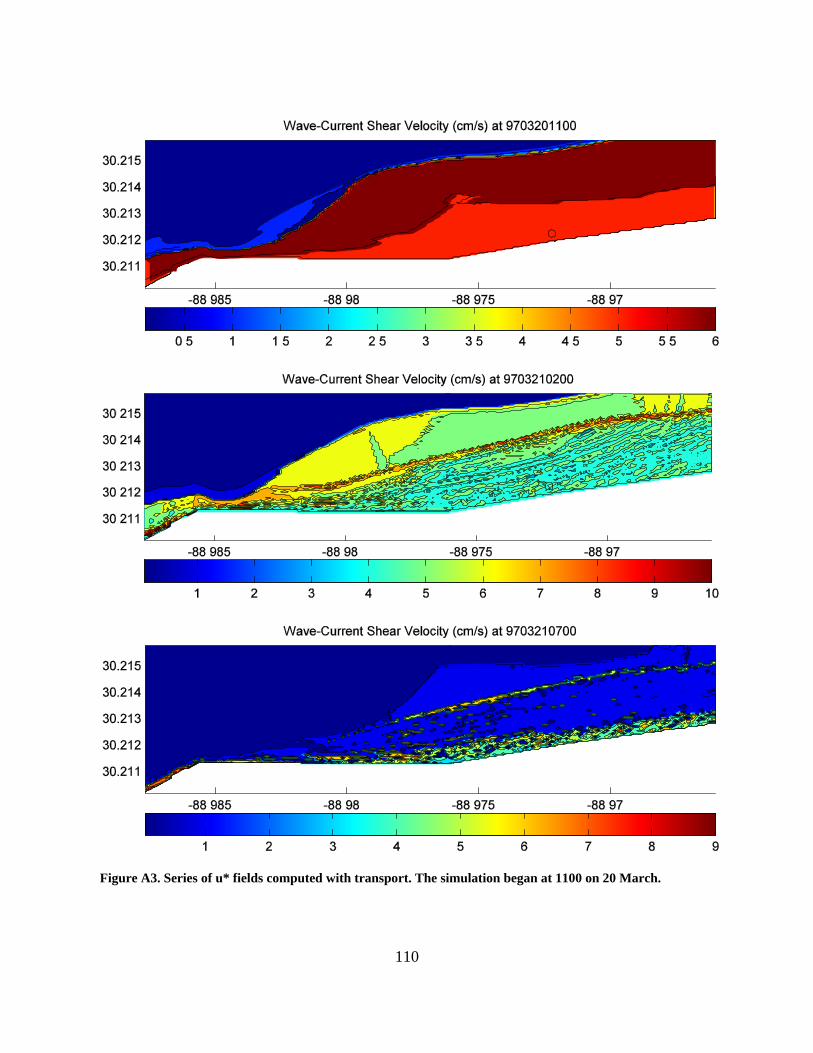
110

Figure A3. Series of u* fields computed with transport. The simulation began at 1100 on 20 March.

111

Figure A4. Initial and 6 hour u* fields with no transport.

112

CLASS BOTTOM TOP MID USTARC TC SETV 1 0.0000020 0.0000029 0.0000024 0.0095625 0.0937265 0.0000020 2 0.0000029 0.0000042 0.0000035 0.0108165 0.1199227 0.0000049 3 0.0000042 0.0000061 0.0000051 0.0122351 0.1534405 0.0000117 4 0.0000061 0.0000090 0.0000074 0.0138397 0.1963264 0.0000279 5 0.0000090 0.0000131 0.0000109 0.0156548 0.2511987 0.0000659 6 0.0000131 0.0000192 0.0000159 0.0177079 0.3214076 0.0001525 7 0.0000192 0.0000282 0.0000233 0.0200302 0.4112395 0.0003444 8 0.0000282 0.0000412 0.0000341 0.0226571 0.5261792 0.0007548 9 0.0000412 0.0000604 0.0000499 0.0256286 0.6732439 0.0015996 10 0.0000604 0.0000884 0.0000730 0.0289897 0.8614123 0.0032660 11 0.0000884 0.0001294 0.0001069 0.0327916 1.1021734 0.0064057 12 0.0001294 0.0001895 0.0001566 0.0370922 1.4102257 0.0120421 13 0.0001895 0.0002774 0.0002293 0.0419567 1.8043773 0.0216625 14 0.0002774 0.0004061 0.0003356 0.0474593 2.3086922 0.0372514 15 0.0004061 0.0005946 0.0004914 0.0536835 2.9539616 0.0612119 16 0.0005946 0.0008706 0.0007195 0.0607239 3.7795801 0.0961377 17 0.0008706 0.0012746 0.0010534 0.0686877 4.8359566 0.1444414 18 0.0012746 0.0018661 0.0015422 0.0776960 6.1875834 0.2079121 19 0.0018661 0.0027321 0.0022579 0.0878856 7.9169841 0.2873289 20 0.0027321 0.0040000 0.0033058 0.099411710.1297464 0.3822823

A

113

SEDIMENT DISTRIBUTION 1 LOW LIMIT UP LIMIT MEAN STD DEV REQUESTED (PHI): 9.0 0.0 4.5 1.5 AVAILABLE (PHI): 9.0 0.2 4.3 1.5 DISTRIBUTION CONTAINS CLASSES 1 TO 16 CLASS DIAMETER (MM) AWP (%) 1 0.00236 0.21 2 0.00346 0.56 3 0.00507 1.33 4 0.00742 2.76 5 0.01086 5.02 6 0.01590 8.00 7 0.02328 11.15 8 0.03408 13.61 9 0.04989 14.55 10 0.07305 13.61 11 0.10695 11.15 12 0.15658 8.00 13 0.22925 5.02 14 0.33564 2.76 15 0.49141 1.33 16 0.71947 0.56 17 1.05336 0.00 18 1.54221 0.00 19 2.25793 0.00 20 3.30580 0.00 TOTAL 99.61

Figure A5. Sediments used in TRANS98 tests. (A) class properties and (B) default sizes.

B

114

Figure A6. Example of the Shields diagram that has been included in TRANS98 for calculating bed properties and sediment entrainment. The upper is more accurate for definitions but the lower has useful annotations. (http://serc.carleton.edu/images/NAGTWorkshops/sedimentary/activities/shields.gif)

03_shields_diagram.gif (GIF Image, 700x371 pixels)http://www.uwsp.edu/geo/faculty/lemke/geomorphology/images/03_shiel...

115

Figure A7. Time series of u* for a run with transport.

116

Figure A8. Time series of ripple heights for the small domain.

117

Figure A9. Predicted variables for a simulation with transport and a constant bed roughness of 1 cm.

118

Figure A10. The east-west component of bed load (left), suspended load (center), and diffusion (right) from independent simulations with all other transport modes turned off. The input currents were interpolated but not smoothed.

119

Figure A11. The east-west component of bedload (left), suspended load (center), and diffusion (right) from independent simulations with all other transport modes turned off. The input currents were interpolated and smoothed 10 times. The diffusion coefficient AH (AHCON in Equation 7) = 5 for the right panel and 0 for the other simulations.

120

Figure A12. Erosion depths for simulation with no smoothing (left), 10 passes (center) and 20 passes (right) of the input currents. Theses simulations included bed load, suspended load, and diffusion (AH = 5). The smoothing was done with a box filter of size 7.

121

Figure A13. Snapshots of the change in bed median grain size.

122

Figure A14. Selected weight percent composition in the deposited sediment after 1 hour (upper panels) and 6 hours (lower panels) for 50 micron (left) and 229 micron (right) size classes.

123

Figure A15. Bed elevation changes after 1 hour for test BF001.

124

Figure A16. Bed elevation changes after 1 hour for test BF002.

125

Figure A17. Bed elevation changes for test BF003.

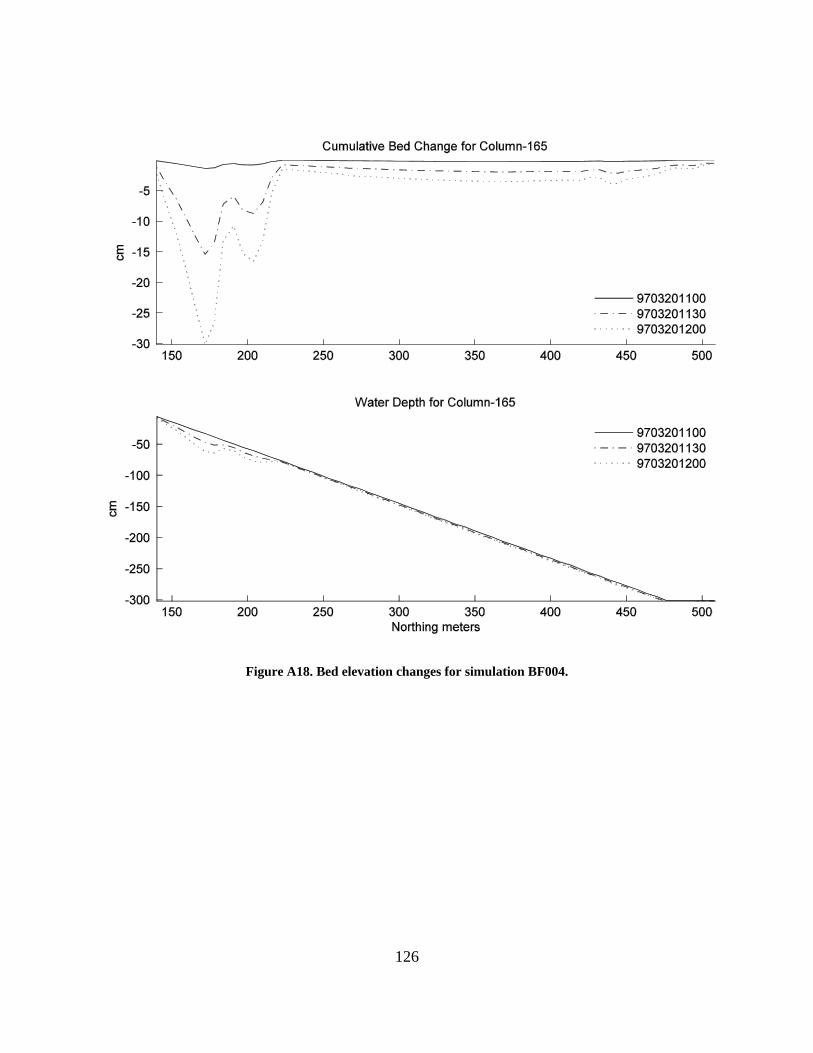
126

Figure A18. Bed elevation changes for simulation BF004.

127

Figure A19. Same as Figure 18 but with a time step 0f 60 s instead of 180 s.

128

Figure A20. Results for seafloor elevation for experiment FM001, which used a small grid with realistic forcing for the north side of Ship Island near Fort Massachusetts. See Appendix B for details.

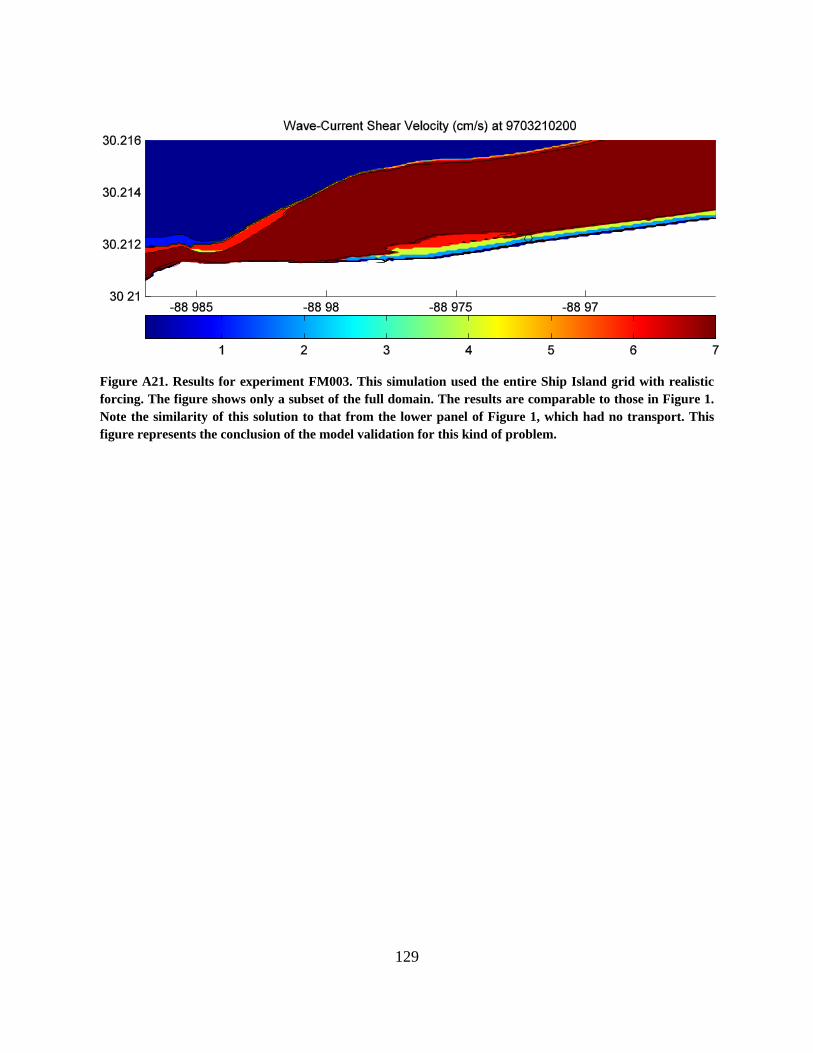
129

Figure A21. Results for experiment FM003. This simulation used the entire Ship Island grid with realistic forcing. The figure shows only a subset of the full domain. The results are comparable to those in Figure 1. Note the similarity of this solution to that from the lower panel of Figure 1, which had no transport. This figure represents the conclusion of the model validation for this kind of problem.

130

Appendix B: TRANS98 Version 3 Testing for Uniform Sediments on Idealized and Realistic Grids

AP

PE

ND

IX B

TR

AN

S98

Ver

sion

3 T

esti

ng f

or U

nifo

rm S

edim

ents

on

Idea

lize

d an

d R

eali

stic

Gri

ds

Tim

othy

R. K

een

6 Ja

nuar

y 20

10

Tab

le B

1 li

sts

sim

ulat

ions

tha

t ar

e de

sign

ed t

o te

st s

ever

al a

spec

ts o

f th

e nu

mer

ical

alg

orit

hms

used

in

calc

ulat

ing

adve

ctio

n of

se

dim

ent a

nd th

e re

sult

ing

chan

ges

in b

ed c

ompo

siti

on a

nd e

leva

tion

. T

his

spec

ific

ally

incl

udes

the

boun

dary

con

diti

ons.

All

of

thes

e si

mul

atio

ns w

ere

com

plet

ed o

n a

sub-

dom

ain

of t

he S

hip

Isla

nd/F

ort M

assa

chus

etts

gri

d. T

his

redu

ced

grid

use

s gr

id c

ells

161

-180

(x

axis

) an

d 21

-80

(y a

xis)

fro

m t

he o

rigi

nal

grid

. T

he r

esul

ts u

sing

the

GC

C c

ompi

ler

wer

e co

mpa

red

to G

95.

The

y w

ere

the

sam

e ex

cept

for

a t

ende

ncy

for

G95

to

wri

te -

0.00

ins

tead

of

0.00

in

prin

tint

.F,

and

for

the

resu

lts

of N

INT

(RE

AL

) to

res

ult

in r

ound

ing

dow

n w

ith

GC

C (

GF

OR

TR

AN

).

Tes

ts U

F00

1 to

UF

004

all p

rodu

ced

the

sam

e re

sult

but

rot

ated

wit

h re

spec

t to

the

land

war

d er

osio

n bo

unda

ry c

ondi

tion

.

Tes

ts U

F00

5 to

UF

008

prod

uced

iden

tica

l res

ults

exc

ept f

or th

e tr

ansp

ort r

ate,

whi

ch m

imic

ked

the

inpu

t flo

w d

irec

tion

.

Tes

ts U

F00

9 to

UF

012

prod

uced

the

sam

e re

sult

but

rot

ated

.

Tes

t B

F00

1 is

com

plex

to

eval

uate

. It

appe

ars

to b

e re

ason

able

as

disc

usse

d in

Tab

le B

2. A

ll o

f th

e re

sult

s ar

e co

nsis

tent

and

the

fil

es

also

sho

w s

imil

ar r

esul

ts.

Thi

s ex

ampl

e co

mpl

etes

tes

ting

of

the

boun

dary

con

diti

ons

and

the

basi

c tr

ansp

ort

algo

rith

m f

or o

ne g

rain

si

ze. I

t wil

l be

appl

ied

to F

t. M

assa

chus

etts

to c

ompl

ete

this

pha

se o

f va

lida

tion

.

Tes

t F

M00

1 de

mon

stra

tes

the

robu

stne

ss o

f th

e m

odel

usi

ng r

eali

stic

(m

odel

ed)

curr

ents

on

a re

al b

each

. The

ove

rall

res

ult

is s

imil

ar

to t

hat

from

the

BF

ser

ies

wit

h a

slig

ht c

ompl

exit

y in

clud

ed b

y th

e di

ffer

ent

dept

hs, c

urre

nts,

and

wav

es. T

he r

esul

ts p

rese

nted

in

this

re

port

dem

onst

rate

that

this

mod

el c

an b

e us

ed f

or s

imil

ar te

sts

wit

h on

e si

ze s

edim

ent o

nly.

Fur

ther

test

ing

is r

equi

red

for

othe

r ca

ses.

131

Tab

le B

1

Test Con

dition

 Nam

e Pa

rameters 

UNIFORM

 FLO

W 

DEPTH

 = con

stant 1

 m; H

S = constant 50 cm

; TM = con

stant 3

 sec; D

T = 18

0 sec; Z

r = 0.5 m

; DURA

TION = 1 hou

r. 

SUSPEN

DED

 _LO

AD = on; BED

_LOAD = off; D

IFFU

SION = off.  Uniform

 D50

 = 73 microns.

BEACH

FACE

 DEPTH

 = flat sectio

n 6 cells wide offsho

re; steady gradient from

 3m to

 0.1m; H

S = constant 50 cm

; TM = 

constant 3 sec; D

T = 18

0 sec; Z

r = 0.5 m

 (or 1/2 water dep

th); DURA

TION = 1 hou

r. SUSPEN

DED

 _LO

AD = on; 

BED_LOAD = off; D

IFFU

SION = off.  

FORT

 MASS 

DEPTH

 = The

 5×6m Ship Island

 grid; HS and TM

 = observatio

ns from

 Fort M

assachusetts pier; DT = 18

0 sec; Z

r = 

0.5 m (o

r 1/2 water dep

th); DURA

TION = 20 ho

ur, starting at 199

7033

0110

0; SUSPEN

DED

 _LO

AD = on; 

BED_LOAD = off; D

IFFU

SION = off. 

    

132

 

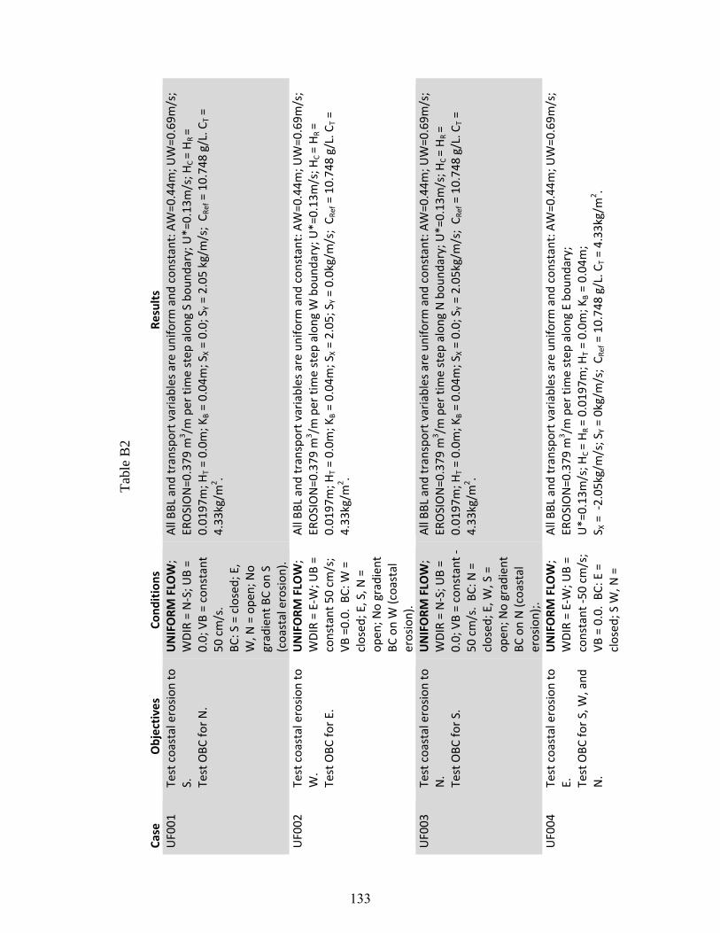
Tab

le B

2

Case 

Objectives 

Cond

itions 

Results 

UF001

 Test coastal erosion

 to 

S. 

Test OBC

 for N.  

UNIFORM

 FLO

W; 

WDIR = N‐S; U

B = 

0.0; VB = constant 

50 cm/s.   

BC: S = closed; E, 

W, N

 = ope

n; No 

gradient BC on

 S 

(coastal erosion

). 

All BB

L and transport variables are uniform

 and

 con

stant: AW=0.44m

; UW=0.69m

/s;  

EROSION=0.379

 m3 /m per time step

 along

 S bou

ndary; U*=0.13

m/s; H

C = HR = 

0.01

97m; H

T = 0.0m

; KB = 0.04

m; S

X = 0.0; S

Y = 2.05

 kg/m/s;  C R

ef = 10.74

8 g/L. C

T = 

4.33

kg/m

2 . 

UF002

 Test coastal erosion

 to 

W. 

Test OBC

 for E.  

UNIFORM

 FLO

W; 

WDIR = E‐W

; UB = 

constant 50 cm

/s; 

VB =0.0.  BC: W

 = 

closed

; E, S, N

 = 

open

; No gradient 

BC on W (coastal 

erosion). 

All BB

L and transport variables are uniform

 and

 con

stant: AW=0.44m

; UW=0.69m

/s;  

EROSION=0.379

 m3 /m per time step

 along

 W bou

ndary; U*=0.13

m/s; H

C = HR = 

0.01

97m; H

T = 0.0m

; KB = 0.04

m; S

X = 2.05

; SY = 0.0kg/m/s;  C R

ef = 10.74

8 g/L. C

T = 

4.33

kg/m

2 . 

UF003

 Test coastal erosion

 to 

N. 

Test OBC

 for S.  

UNIFORM

 FLO

W; 

WDIR = N‐S; U

B = 

0.0; VB = constant ‐

50 cm/s.  BC

: N = 

closed

; E, W

, S = 

open

; No gradient 

BC on N (coastal 

erosion);. 

All BB

L and transport variables are uniform

 and

 con

stant: AW=0.44m

; UW=0.69m

/s;  

EROSION=0.379

 m3 /m per time step

 along

 N bou

ndary; U*=0.13

m/s; H

C = HR = 

0.01

97m; H

T = 0.0m

; KB = 0.04

m; S

X = 0.0; S

Y = 2.05

kg/m

/s;  C R

ef = 10.74

8 g/L. C

T = 

4.33

kg/m

2 . 

UF004

 Test coastal erosion

 to 

E. 

Test OBC

 for S, W

, and

 N.  

UNIFORM

 FLO

W; 

WDIR = E‐W

; UB = 

constant ‐50

 cm/s; 

VB = 0.0.  BC

: E = 

closed

; S W

, N = 

All BB

L and transport variables are uniform

 and

 con

stant: AW=0.44m

; UW=0.69m

/s;   

EROSION=0.379

 m3 /m per time step

 along

 E bou

ndary;  

U*=0.13

m/s; H

C = HR = 0.01

97m; H

T = 0.0m

; KB = 0.04

m;  

S X =  ‐2.05

kg/m

/s; S

Y = 0kg/m/s;  C R

ef = 10.74

8 g/L. C

T = 4.33

kg/m

2 . 

133

open

; No gradient 

BC on E (coastal 

erosion). 

UF005

 Test all op

en 

boun

daries. 

UNIFORM

 FLO

W; 

WDIR = E‐W

; UB = 

constant 50 cm

/s; 

VB =0. BC:  E, W

, N, 

S= ope

n 

All BB

L and transport variables are uniform

 and

 con

stant: AW=0.44m

; UW=0.69m

/s;  

EROSION=n

one;  

U*=0.13

m/s; H

C = HR = 0.01

97m; H

T = 0.0m

; KB = 0.04

m;  

S X = ‐2.05

kg/m

/s; S

Y = 0kg/m/s;  C R

ef = 10.74

8 g/L. C

T = 4.33

kg/m

2 . 

UF006

 Test all op

en 

boun

daries. 

UNIFORM

 FLO

W; 

WDIR = E‐W

; UB = 

constant ‐50

 cm/s.  

BC: S, N

, E, W

 = 

open

 

All BB

L and transport variables are uniform

 and

 con

stant: AW=0.44m

; UW=0.69m

/s;  

EROSION=n

one;  

U*=0.13

m/s; H

C = HR = 0.01

97m; H

T = 0.0m

; KB = 0.04

m;  

S X = 2.05kg/m/s; S

Y = 0kg/m/s;  C R

ef = 10.74

8 g/L. C

T = 4.33

kg/m

2 . 

UF007

 Test all op

en 

boun

daries. 

UNIFORM

 FLO

W; 

WDIR = E‐W

; UB = 

0.0; VB = constant ‐

50 cm/s.   

BC: E, W

, S, N

 = 

open

 

All BB

L and transport variables are uniform

 and

 con

stant: AW=0.44m

; UW=0.69m

/s;  

EROSION=n

one;  

U*=0.13

m/s; H

C = HR = 0.01

97m; H

T = 0.0m

; KB = 0.04

m;  

S X = 0.0kg/m

/s; S

Y = ‐2.05kg/m/s;  C R

ef = 10.74

8 g/L. C

T = 4.33

kg/m

2 . 

UF008

 Test all op

en 

boun

daries. 

UNIFORM

 FLO

W; 

WDIR = E‐W

; UB = 

constant 50 cm

/s; 

VB =0.0.   

BC: E, W

 = closed; 

S, N = ope

n 

All BB

L and transport variables are uniform

 and

 con

stant: AW=0.44m

; UW=0.69m

/s;  

EROSION=n

one;  

U*=0.13

m/s; H

C = HR = 0.01

97m; H

T = 0.0m

; KB = 0.04

m;  

S X = 0.0kg/m

/s; S

Y = 2.05

kg/m

/s;  C R

ef = 10.74

8 g/L. C

T = 4.33

kg/m

2 . 

UF009

 Test erosion

 on N and

 de

positio

n on

 S. 

UNIFORM

 FLO

W; 

WDIR = N‐S; U

B = 

0.0; VB = constant ‐

50 cm/s.   

BC: E, W

 = ope

n; S, 

N = closed. No 

land

ward erosion 

(BOUND=0). 

EROSION: The

 cum

ulative erosion de

pth at th

e leew

ard en

d of th

e grid steadily 

increases in increm

ents of 3

 cm per time step

.   

SEABE

D: The

 seaflo

or change = ‐3cm

 upw

ind and +3cm

 dow

nwind.  The

 bed

 thickness (1 time step

) = 3cm

 at d

ownw

ind en

d.  A

ll othe

r pred

icted variables are the 

same as UF003

. No coastal erosion

 calculated. 

The seafloor elevatio

n (SEA

BED) reaches ‐63

cm/+63

 cm at the

 upw

ind /dow

nwind 

ends of the

 grid after 20

 time step

s. This is alarm

ing grow

th but expected for the 

algorithm, w

hich doe

s no

t allow a change in bed

 com

positio

n with

 erosion

.   

134

UF010

 Test erosion

 on E and 

depo

sitio

n on

 W 

UNIFORM

 FLO

W; 

WDIR = E‐W

; UB = 

constant ‐50

 cm/s; 

VB =  0.0. 

BC: N

, S = ope

n; E, 

W = closed. No 

land

ward erosion 

(BOUND=0). 

EROSION: The

 cum

ulative erosion de

pth at th

e leew

ard en

d of th

e grid steadily 

increases in increm

ents of 3

.45 cm

 per time step

.   

SEABE

D: The

 seaflo

or change = ‐3.45cm upw

ind and +3.45cm dow

nwind.  The

 bed

 thickness (1 time step

) = 3.45cm at d

ownw

ind en

d.  A

ll othe

r pred

icted variables are 

the same as UF004

. The

 magnitude

s are slightly larger th

an UF009

 because dy = 6m

 and dx = 5m. N

o coastal erosion

 calculated. 

The seafloor elevatio

n (SEA

BED) reaches ‐72

cm/+72

 cm at the

 upw

ind /dow

nwind 

ends of the

 grid after 20

 time step

s. This is alarm

ing grow

th but expected for the 

algorithm, w

hich doe

s no

t allow a change in bed

 com

positio

n with

 erosion

. UF011

 Test erosion

 on S and 

depo

sitio

n on

 N 

UNIFORM

 FLO

W; 

WDIR = N‐S; U

B = 

0.0; VB = constant 

50 cm/s.   

BC: E, W

 = ope

n; S, 

N = closed. No 

land

ward erosion 

(BOUND=0). 

The results are exactly th

e same as UF009

, excep

t turne

d 18

0 de

g., w

ith erosion

 on S 

and de

positio

n on

 N.  No coastal erosion

 calculated. 

UF012

 Test erosion

 on W and

 de

positio

n on

 E 

UNIFORM

 FLO

W; 

WDIR = E‐W

; UB = 

constant 50 cm

/s; 

VB =  0.0. 

BC: N

, S = ope

n; E, 

W = closed. No 

land

ward erosion 

(BOUND=0). 

The results are exactly th

e same as UF010

, excep

t turne

d 18

0 de

g., w

ith erosion

 on 

W and

 dep

osition

 on E. No coastal erosion

 calculated. 

BF00

1 Test sho

aling wave 

resuspen

sion

 and

 transport. 

Dep

osition at th

e coast. 

BEACH

FACE

; WDIR 

= N‐S; U

B = 0.0; VB 

= constant 20 cm

/s.  

BC: E, W

 = ope

n; S, 

N = closed. No 

land

ward erosion 

(BOUND=0). 

Uniform

 D50

 = 73 

microns. 

EROSION:  Th

e cumulative erosion de

pth at th

e S en

d (offshore) rem

ains con

stant (~ 

4 mm) for 30 min and

 then

 con

tinue

s to increase by ~4

 mm per 1/2 hou

r. At the

 toe 

of th

e be

ach (w

here gradien

t begins) (~

j=27

), erosion be

gins to

 increase ~ 2.5mm/ 

cell and reache

s 10

8mm at j=65 bu

t more land

ward cells are filled in by sedimen

t. 

Maxim

um erosion

 (230

mm) after 1 hr is at J=63 with

 land

 exten

ding

 to J=

65.  

SEABE

D: The

 new

 algorith

m allows wet cells to

 becom

e land

 if filled in (i.e., thktot > 

depth). B

y 1 ho

ur, row

 79 has be

come land

. The

 seaflo

or change at 1 hr indicates 

<1mm erosion

 offshore and a steady

 increase to

 23cm at J=63. After 1 hr, row

 66 has 

221m

m of d

eposition

. The

 cum

ulative be

d elevation at 1 hou

r indicates erosion at 

135

400m

 has filled in th

e last row

 (79) and

 con

structed

 a bar with

 a m

axim

um elevatio

n of 60 cm

 at 4

40m. N

o coastal erosion

 was calculated be

cause of dep

osition

 at the

 do

wnw

ind coast.  

CONCE

NTR

ATION: The

 suspe

nded

 sed

imen

t con

centratio

n sm

oothly increases 

land

ward. It is relatively constant with

 height u

ntil the be

ach toe, whe

re it begins to 

increase. The

 volum

e fractio

n at th

e offsho

re bou

ndary ranges from

 10‐

2.7  to 10‐

3  at 

z=0 and 26

. The

 con

centratio

n increases land

ward and be

comes m

ore un

iform

 with

 de

pth, reaching 10

‐1.7 (z=0) and

 10‐

1.8  (z=26) at land at 1 hou

r. All variables are 

constant along

 row

s.  

The suspen

ded transport rate increases sm

oothly fo

rm 5.3 kg/m/s offshore to a 

maxim

um of 1

1.2 at row

 66 at th

e start o

f the

 run

. By 30

 min, the

 coast has m

igrated 

offsho

re and

 SY reache

s 10

.6 kg/m/s at row

 65. By 1 ho

ur S

Y de

creases to a m

ax of 9

.9 

kg/m

/s at row

 63.  

BF00

2 Test sho

aling wave 

resuspen

sion

 and

 transport. 

Erosion ne

ar th

e coast.  

BEACH

FACE

; WDIR 

= N‐S; U

B = 0.0; VB 

= increasing

 seaw

ard from

   ‐20 

cm/s to

 ‐50

 cm/s at 

the op

en 

boun

dary.   

BC: E, W

 = ope

n; S, 

N = closed. No 

land

ward erosion 

(BOUND=0). 

Uniform

 D50

 = 73 

microns. 

EROSION:  Th

e cumulative erosion de

pth at th

e N end

 (420

m) reaches 13 mm in

 the 

first time step

 and

 increases to 15cm at 3

0 min, and

 30 cm

 at 1

 hou

r. Erosion

 increases to a m

axim

um at ~

 80 m from

 the coast  

SEABE

D: The

 new

 algorith

m doe

s no

t make land

 ce lls wet if erosion

 is excessive; thu

s erosion exceed

s 15

cm per half‐ho

ur near the coast. The

 seaflo

or change at 1 hr 

indicates <5cm

 erosion

 everywhe

re with

in th

e mod

el grid be

cause of th

e no

‐gradien

t seaw

ard bo

undary; i.e., mass is lost from

 the do

main.  

CONCE

NTR

ATION: The

 suspe

nded

 sed

imen

t con

centratio

n is a m

inim

um of 0

.4 kg/m

2  at th

e coast a

nd increases seaw

ard for the first 60 m (~

14 kg/m

2 ) before de

creasing

 mon

oton

ously to 9 kg/m

2  at th

e offsho

re bou

ndary. The

 total loa

d varies little from

 the coast to 20

 m offshore with

 time as th

e water dep

th.  Th

e 3D

 con

centratio

n de

creases with

 height e

verywhe

re excep

t at the

 coast, w

here it is <1%

 by volume. 

Furthe

r offsho

re, the

 near‐be

d and surface values are 10‐

2.2  and 10

‐2.5 kg/m

3 , 

respectiv

ely. The

 volum

e fractio

n at th

e offsho

re bou

ndary ranges from

 2% to

 0.1% 

at z=0

 and

 26. All variables are constant along

 row

s.  

The suspen

ded transport rate increases sm

oothly seaward from

 0.3 kg/m/s at the

 coast to a maxim

um of 5

.3 kg/m/s at the

 seaward bo

undary at the

 start of the

 run

. By

 30 min, S

Y reache

s 0.18

 kg/m/s at row

 78 be

cause of th

e increasing

 water dep

th. 

Furthe

r erosion at th

e coast results in

 SY increasing

 to 0.19 kg/m

/s by 1 ho

ur. 

BF00

3 Test sho

aling wave 

resuspen

sion

 and

 BE

ACH

FACE

; WDIR 

= N‐S; U

B = 0.0; VB 

EROSION:  Th

e cumulative erosion de

pth at th

e N end

 (onsho

re) reaches 0.3mm in

 30 

min, w

hich is th

e sm

allest amou

nt in

 the grid because of m

aterial erode

d from

 land

. 

136

transport. 

Coastal erosion

 land

ward bo

undary 

with

 no‐gradient 

transport a

t coast.  

= increasing

 seaw

ard from

   ‐20 

cm/s to

 ‐50

 cm/s at 

the op

en 

boun

dary.   

BC: E, W

 = ope

n; S 

= closed

; N = 

Land

ward erosion 

(BOUND=1). 

Uniform

 D50

 = 73 

microns. 

A m

axim

um of 1

4mm is erode

d at row

 73.  Erosion

 occurs across th

e shore face with

 a max of ~

3cm at ~

200m

 from

 offshore. Erosion

 doe

s no

t occur at the

 seaward 

boun

dary because it is ope

n. 

SEABE

D: D

espite sed

imen

t inp

ut from

 the coast, a 30cm trou

gh was erode

d ~30m

 from

 the coast w

ith a 2cm

 “bar” dep

osite

d just seaward on

 the ne

wly erode

d surface.  

CONCE

NTR

ATION: The

 sed

imen

t con

centratio

n is very similar to BF002

. 

BF00

4 Test sho

aling wave 

resuspen

sion

 and

 transport. 

Coastal erosion

 land

ward bo

undary 

with

 no‐gradient 

BEACH

FACE

; WDIR 

= N‐S; U

B = 0.0; VB 

= increasing

 seaw

ard from

   20

 cm

/s to

 50 cm

/s at 

the op

en 

This experim

ent w

as designe

d to te

st th

e land

ward bo

undary con

ditio

n as im

posed 

on th

e south/west, because of the

 com

putatio

n of transports at i+1/2, j+1/2.  Th

e result was sym

metrical to BF00

3 with

 a fe

w m

inor differen

ces cause by

 a slight 

differen

ce in

 the im

posed wave fie

ld.  

137

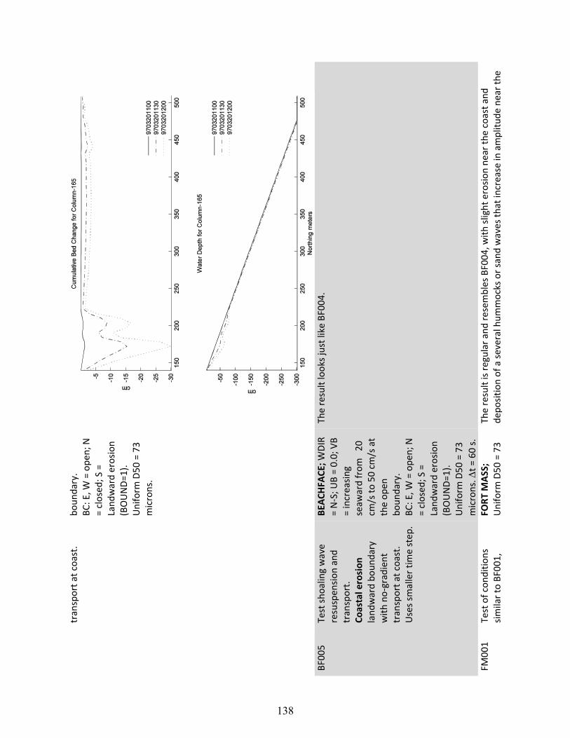
transport a

t coast.  

boun

dary.   

BC: E, W

 = ope

n; N 

= closed

; S = 

Land

ward erosion 

(BOUND=1). 

Uniform

 D50

 = 73 

microns. 

BF00

5 Test sho

aling wave 

resuspen

sion

 and

 transport. 

Coastal erosion

 land

ward bo

undary 

with

 no‐gradient 

transport a

t coast.  

Uses sm

aller tim

e step

. 

BEACH

FACE

; WDIR 

= N‐S; U

B = 0.0; VB 

= increasing

 seaw

ard from

   20

 cm

/s to

 50 cm

/s at 

the op

en 

boun

dary.   

BC: E, W

 = ope

n; N 

= closed

; S = 

Land

ward erosion 

(BOUND=1). 

Uniform

 D50

 = 73 

microns. 

t = 60 s. 

The result looks just like BF004

. 

FM00

1 Test of con

ditio

ns 

similar to BF001

, FO

RT M

ASS;   

Uniform

 D50

 = 73 

The result is regular and

 resem

bles BF004

, with

 slight erosion

 near the coast a

nd 

depo

sitio

n of a several hum

mocks or sand

 waves th

at increase in

 amplitu

de near the 

138

BF00

3 and BF00

4—de

positio

n and erosion 

from

 the coast. 

microns. 

coast.  The

se scour pits are located at 240

m, 300

m, 360

m, and

 420

m. The

 regular 

spacing of ~60

m suggests there may be a correlation with

 the interpolated

 currents 

from

 POM, w

hich were on

 a grid with

 spacing

 of ~

800m

. The

 merged fie

lds from

 PO

M and

 Sho

recirc were sm

oothed

 50  tim

es fo

r this experim

ent, which wou

ld have 

created a differen

t effect than the original spacing. 

 Their causes can

 be seen

 in a m

ultip

lot o

f several variables along

 row

 168

. The

 N‐S 

curren

ts con

tain steps at 3

60m and

 410

m, w

hich increased the TSS and thus SLT at 

these locatio

ns. The

se are probably artificial and

 caused by

 the interpolated

 currents. 

The scou

r at 300

m is caused by

 the sharp increase in

 she

ar stress and transport rate 

at th

e toe of th

e be

ach. Finally, the

 scour at the

 coast (2

40m) is caused

 by the 

extrem

ely shallow water th

ere. It was noted

 in App

endix A th

at th

ere was a lot o

f no

ise in th

e curren

ts from

 Sho

recirc. This was greatest in the first time step

 (970

3201

100) and

 con

tributed

 to noise at 3

60m and

 420

m. The

 later fie

lds were 

much sm

oother but th

e scou

r ho

les could no

t be filled in th

e simulation.  

139

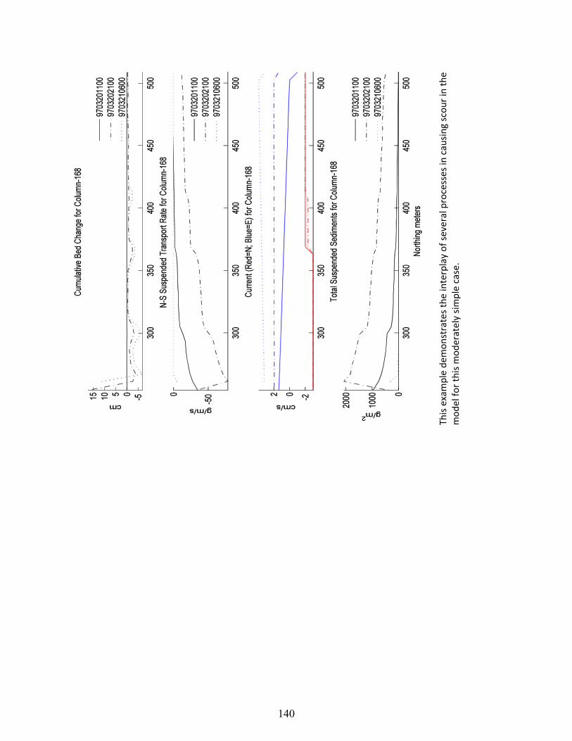
  This example de

mon

strates the interplay of several processes in

 causing

 scour in

 the 

mod

el fo

r this m

oderately simple case.  

 

140