The CN2 Induction Algorithm - Brigham Young...
23
Machine Learning 3: 261-283, 1989 © 1989 Kluwer Academic Publishers - Manufactured in The Netherlands The CN2 Induction Algorithm PETER CLARK ([email protected]) TIM NIBLETT ([email protected]) The Turing Institute, 36 North Hanover Street, Glasgow, G1 2AD, U.K. (Received: June 25, 1987) (Revised: October 25, 1988) Keywords: Concept learning, rule induction, noise, comprehensibility Abstract. Systems for inducing concept descriptions from examples are valuable tools for assisting in the task of knowledge acquisition for expert systems. This paper presents a description and empirical evaluation of a new induction system, CN2, designed for the efficient induction of simple, comprehensible production rules in domains where problems of poor description language and/or noise may be present. Implementations of the CN2, ID3, and AQ algorithms are compared on three medical classification tasks. 1. Introduction In the task of constructing expert systems, methods for inducing concept de- scriptions from examples have proved useful in easing the bottleneck of knowl- edge acquisition (Mowforth, 1986). Two families of systems, based on the ID3 (Quinlan, 1983) and AQ (Michalski, 1969) algorithms, have been especially successful. These basic algorithms assume no noise in the domain, searching for a concept description that classifies training data perfectly. However, ap- plication to real-world domains requires methods for handling noisy data. In particular, one needs mechanisms that do not overfit the induced concept de- scription to the data, and this requires relaxing the constraint that the induced description must classify the training data perfectly. Fortunately, the ID3 algorithm lends itself to such modification by the na- ture of its general-to-specific search. Tree-pruning techniques (e.g., Quinlan, 1987a; Niblett, 1987), used for example in C4 (Quinlan, Compton, Horn, & Lazarus, 1987) and ASSISTANT (Kononenko, Bratko, & Roskar, 1984), have proved effective against overfitting. However, the AQ algorithm's dependence on specific training examples during search makes it less easy to modify. Ex- isting implementations, such as AQll (Michalski & Larson, 1983) and AQ15 (Michalski, Mozetic, Hong, & Lavrac, 1986), leave the basic AQ algorithm intact and handle noise with pre-processing and post-processing techniques. Our objective in designing CN2 was to modify the AQ algorithm itself in ways that removed this dependence on specific examples and increased the
Transcript of The CN2 Induction Algorithm - Brigham Young...
Machine Learning 3: 261-283, 1989© 1989 Kluwer Academic Publishers - Manufactured in The Netherlands
The CN2 Induction Algorithm
PETER CLARK ([email protected])TIM NIBLETT ([email protected])The Turing Institute, 36 North Hanover Street, Glasgow, G1 2AD, U.K.
(Received: June 25, 1987)(Revised: October 25, 1988)
Keywords: Concept learning, rule induction, noise, comprehensibility
Abstract. Systems for inducing concept descriptions from examples are valuabletools for assisting in the task of knowledge acquisition for expert systems. Thispaper presents a description and empirical evaluation of a new induction system,CN2, designed for the efficient induction of simple, comprehensible production rulesin domains where problems of poor description language and/or noise may be present.Implementations of the CN2, ID3, and AQ algorithms are compared on three medicalclassification tasks.
1. IntroductionIn the task of constructing expert systems, methods for inducing concept de-
scriptions from examples have proved useful in easing the bottleneck of knowl-edge acquisition (Mowforth, 1986). Two families of systems, based on the ID3(Quinlan, 1983) and AQ (Michalski, 1969) algorithms, have been especiallysuccessful. These basic algorithms assume no noise in the domain, searchingfor a concept description that classifies training data perfectly. However, ap-plication to real-world domains requires methods for handling noisy data. Inparticular, one needs mechanisms that do not overfit the induced concept de-scription to the data, and this requires relaxing the constraint that the induceddescription must classify the training data perfectly.
Fortunately, the ID3 algorithm lends itself to such modification by the na-ture of its general-to-specific search. Tree-pruning techniques (e.g., Quinlan,1987a; Niblett, 1987), used for example in C4 (Quinlan, Compton, Horn, &Lazarus, 1987) and ASSISTANT (Kononenko, Bratko, & Roskar, 1984), haveproved effective against overfitting. However, the AQ algorithm's dependenceon specific training examples during search makes it less easy to modify. Ex-isting implementations, such as AQll (Michalski & Larson, 1983) and AQ15(Michalski, Mozetic, Hong, & Lavrac, 1986), leave the basic AQ algorithmintact and handle noise with pre-processing and post-processing techniques.Our objective in designing CN2 was to modify the AQ algorithm itself inways that removed this dependence on specific examples and increased the

262 P. CLARK AND T. NIBLETT
space of rules searched. This lets one apply statistical techniques, analogousto those used for tree pruning, in the generation of if-then rules, leading to asimpler induction algorithm.
One can identify several requirements that learning systems should meet ifthey are to prove useful in a variety of real-world situations:
• Accurate classification. The induced rules should be able to classify newexamples accurately, even in the presence of noise.
• Simple rules. For the sake of comprehensibility, the induced rules shouldbe as short as possible. However, when noise is present, overfitting canlead to long rules. Thus, to induce short rules, one must usually relaxthe requirement that the induced rules be consistent with all the trainingdata. The choice of how much to relax this requirement involves a trade-offbetween accuracy and simplicity (Iba, Wogulis, & Langley, 1988).
• Efficient rule generation. If one expects to use large example sets, it isimportant that the algorithm scales up to complex situations. In practice,the time taken for rule generation should be linear in the size of theexample set.
With these requirements in mind, this paper presents a description and empir-ical evaluation of CN2, a new induction algorithm. This system combines theefficiency and ability to cope with noisy data of ID3 with the if-then rule formand flexible search strategy of the AQ family. The representation for rulesoutput by CN2 is an ordered set of if-then rules, also known as a decisionlist (Rivest, 1987). CN2 uses a heuristic function to terminate search duringrule construction, based on an estimate of the noise present in the data. Thisresults in rules that may not classify all the training examples correctly, butthat perform well on new data.
In the following section we describe CN2 and three other systems used forour comparative study. In Section 3 we consider the time complexity of thevarious algorithms and in Section 4 we compare their performance on threemedical diagnosis tasks. We also compare the performance of ASSISTANT andCN2 on two synthetic tasks. In Section 5 we discuss the significance of ourresults, and we follow this with some suggestions for future work in Section 6.
2. CN2 and related algorithmsCN2 incorporates ideas from both Michalski's (1969) AQ and Quinlan's
(1983) ID3 algorithms. Thus we begin by describing Kononenko et al.'s (1984)ASSISTANT, a variant of ID3, and AQR, the authors' reconstruction of Michal-ski's method. After this, we present CN2 and discuss its relationship to thesesystems. We also describe a simple Bayesian classifier, which provides a refer-ence for the performance of the other algorithms. We characterize each systemalong three dimensions:
• the representation language for the induced knowledge;• the performance engine for executing the rules; and• the learning algorithm and its associated search heuristics.
THE CN2 ALGORITHM 263
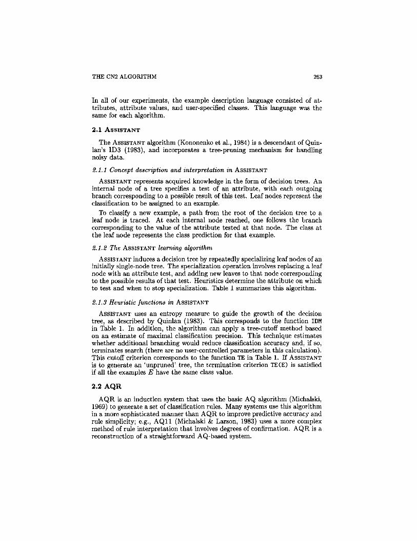
In all of our experiments, the example description language consisted of at-tributes, attribute values, and user-specified classes. This language was thesame for each algorithm.
2.1 ASSISTANT
The ASSISTANT algorithm (Kononenko et al., 1984) is a descendant of Quin-lan's ID3 (1983), and incorporates a tree-pruning mechanism for handlingnoisy data.
2.1.1 Concept description and interpretation in ASSISTANTASSISTANT represents acquired knowledge in the form of decision trees. An
internal node of a tree specifies a test of an attribute, with each outgoingbranch corresponding to a possible result of this test. Leaf nodes represent theclassification to be assigned to an example.
To classify a new example, a path from the root of the decision tree to aleaf node is traced. At each internal node reached, one follows the branchcorresponding to the value of the attribute tested at that node. The class atthe leaf node represents the class prediction for that example.
2.1.2 The ASSISTANT learning algorithmASSISTANT induces a decision tree by repeatedly specializing leaf nodes of an
initially single-node tree. The specialization operation involves replacing a leafnode with an attribute test, and adding new leaves to that node correspondingto the possible results of that test. Heuristics determine the attribute on whichto test and when to stop specialization. Table 1 summarizes this algorithm.
2.1.3 Heuristic functions in ASSISTANTASSISTANT uses an entropy measure to guide the growth of the decision
tree, as described by Quinlan (1983). This corresponds to the function IDMin Table 1. In addition, the algorithm can apply a tree-cutoff method basedon an estimate of maximal classification precision. This technique estimateswhether additional branching would reduce classification accuracy and, if so,terminates search (there are no user-controlled parameters in this calculation).This cutoff criterion corresponds to the function TE in Table 1. If ASSISTANTis to generate an 'unpruned' tree, the termination criterion TE(E) is satisfiedif all the examples E have the same class value,
2.2 AQR
AQR is an induction system that uses the basic AQ algorithm (Michalski,1969) to generate a set of classification rules. Many systems use this algorithmin a more sophisticated manner than AQR to improve predictive accuracy andrule simplicity; e.g., AQ11 (Michalski & Larson, 1983) uses a more complexmethod of rule interpretation that involves degrees of confirmation. AQR is areconstruction of a straightforward AQ-based system.
264 P. CLARK AND T. NIBLETT
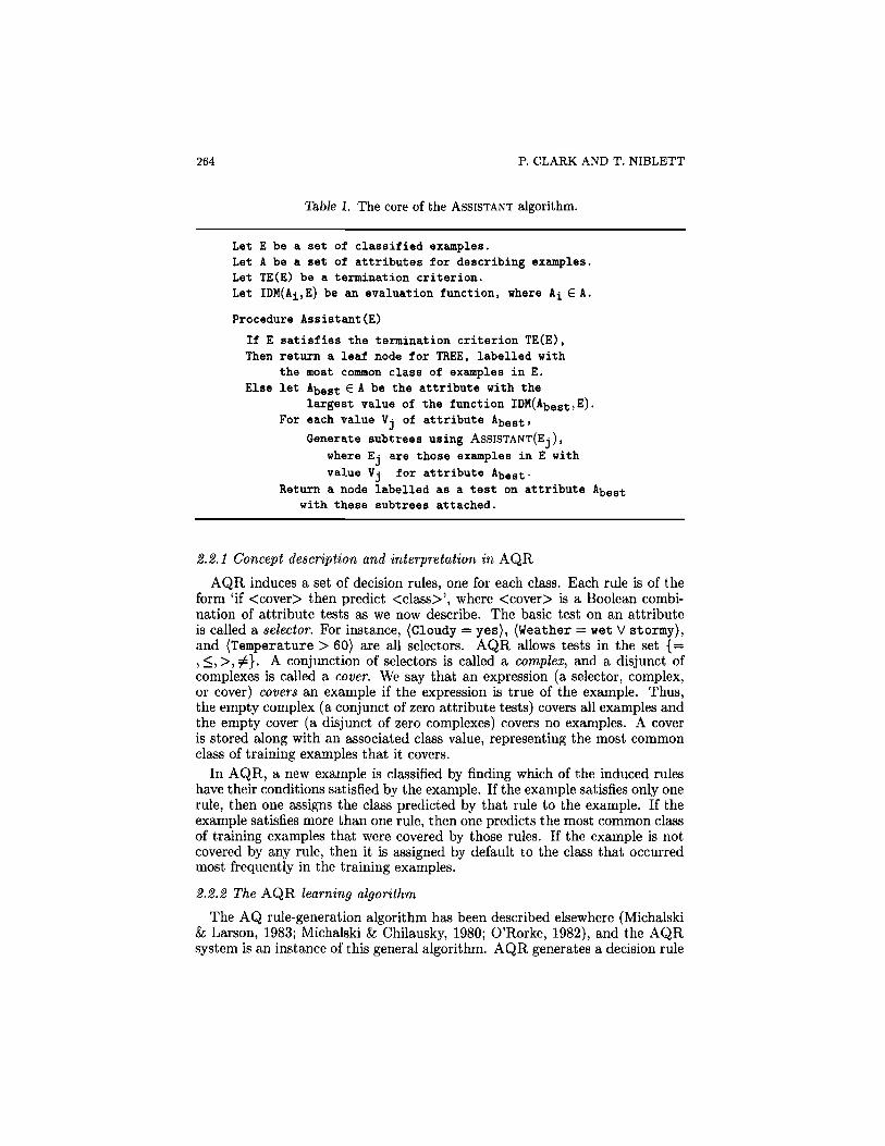
Table 1. The core of the ASSISTANT algorithm.
Let E be a set of classified examples.Let A be a set of attributes for describing examples.Let TE(E) be a termination criterion.Let IDM(Ai,E) be an evaluation function, where Ai 6 A.
Procedure Assistant (E)If E satisfies the termination criterion TE(E) ,Then return a leaf node for TREE, labelled with
the most common class of examples in E.Else let Abest € A be the attribute with the
largest value of the function IDM(Abest,E).For each value Vj of attribute Abest,
Generate subtrees using ASSISTANT(Ej),where Ej are those examples in E withvalue Vj for attribute Abest.
Return a node labelled as a test on attribute Abestwith these subtrees attached.
2.2.1 Concept description and interpretation in AQRAQR induces a set of decision rules, one for each class. Each rule is of the
form 'if <cover> then predict <class>', where <cover> is a Boolean combi-nation of attribute tests as we now describe. The basic test on an attributeis called a selector. For instance, (Cloudy = yes), (Weather = wet V stormy),and (Temperature > 60} are all selectors. AQR allows tests in the set {=,<,>,T^}. A conjunction of selectors is called a complex, and a disjunct ofcomplexes is called a cover. We say that an expression (a selector, complex,or cover) covers an example if the expression is true of the example. Thus,the empty complex (a conjunct of zero attribute tests) covers all examples andthe empty cover (a disjunct of zero complexes) covers no examples. A coveris stored along with an associated class value, representing the most commonclass of training examples that it covers.
In AQR, a new example is classified by finding which of the induced ruleshave their conditions satisfied by the example. If the example satisfies only onerule, then one assigns the class predicted by that rule to the example. If theexample satisfies more than one rule, then one predicts the most common classof training examples that were covered by those rules. If the example is notcovered by any rule, then it is assigned by default to the class that occurredmost frequently in the training examples.
2.2.2 The AQR learning algorithmThe AQ rule-generation algorithm has been described elsewhere (Michalski
& Larson, 1983; Michalski & Chilausky, 1980; O'Rorke, 1982), and the AQRsystem is an instance of this general algorithm. AQR generates a decision rule
THE CN2 ALGORITHM 265
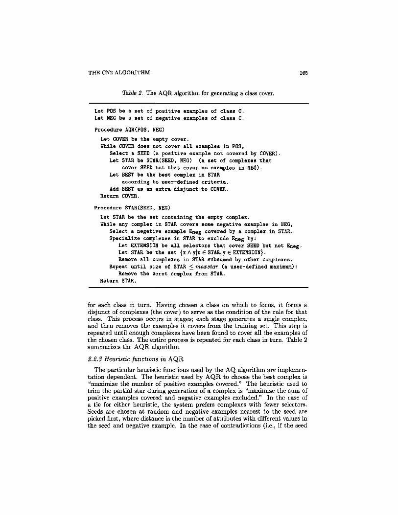
Table 2. The AQR algorithm for generating a class cover.
Let POS be a set of positive examples of class C.Let NEG be a set of negative examples of class C.
Procedure AQR(POS, NEG)Let COVER be the empty cover.While COVER does not cover all examples in POS,
Select a SEED (a positive example not covered by COVER) .Let STAR be STAR (SEED, NEG) (a set of complexes that
cover SEED but that cover no examples in NEG).Let BEST be the best complex in STAR
according to user-defined criteria.Add BEST as an extra disjunct to COVER.
Return COVER.
Procedure STAR(SEED, NEG)Let STAR be the set containing the empty complex.While any complex in STAR covers some negative examples in NEG,
Select a negative example Eneg covered by a complex in STAR.Specialize complexes in STAR to exclude Eneg by:
Let EXTENSION be all selectors that cover SEED but not Eneg.Let STAR be the set {x Ay|x € STAR,y 6 EXTENSION}.Remove all complexes in STAR subsumed by other complexes.
Repeat until size of STAR < max star (a user-defined maximum):Remove the Worst complex from STAR.
Return STAR.
for each class in turn. Having chosen a class on which to focus, it forms adisjunct of complexes (the cover) to serve as the condition of the rule for thatclass. This process occurs in stages; each stage generates a single complex,and then removes the examples it covers from the training set. This step isrepeated until enough complexes have been found to cover all the examples ofthe chosen class. The entire process is repeated for each class in turn. Table 2summarizes the AQR algorithm.
2.2.3 Heuristic functions in AQRThe particular heuristic functions used by the AQ algorithm are implemen-
tation dependent. The heuristic used by AQR to choose the best complex is"maximize the number of positive examples covered." The heuristic used totrim the partial star during generation of a complex is "maximize the sum ofpositive examples covered and negative examples excluded." In the case ofa tie for either heuristic, the system prefers complexes with fewer selectors.Seeds are chosen at random and negative examples nearest to the seed arepicked first, where distance is the number of attributes with different values inthe seed and negative example. In the case of contradictions (i.e., if the seed
266 P. CLARK AND T. NIBLETT
and negative example have identical attribute values) the negative example isignored and a different one is chosen, since the complex cannot be specializedto exclude it but still include the seed.
2.3 The CN2 algorithmNow that we have reviewed ASSISTANT and AQR, we can turn to CN2, a
new algorithm that combines aspects of both methods. We begin by describinghow the general approach arises naturally from consideration of the decision-tree and AQ algorithms and then consider its details.
2.3.1. Relation to ID3 and AQID3 can be easily adapted to handle noisy data by virtue of its top-down
approach to tree generation. During induction, all possible attribute tests areconsidered when 'growing' a leaf node in the tree, and entropy is used to selectthe best one to place at that node. Overfitting of decision trees can thus beavoided by halting tree growth when no more significant information can begained. We wish to apply a similar method to the induction of if-then rules.
The AQ algorithm, when generating a complex, also performs a general-to-specific search for the best complex. However, the method only considersspecializations that exclude some particular covered negative example fromthe complex while ensuring some particular 'seed' positive example remainscovered, iterating until all negative examples are excluded. As a result, AQsearches only the space of complexes that are completely consistent with thetraining data. The basic algorithm employs a beam search, which can beviewed as several hill-climbing searches in parallel.
For the CN2 algorithm, we have retained the beam search method of theAQ algorithm but removed its dependence on specific examples during searchand extended its search space to include rules that do not perform perfectlyon the training data. This is achieved by broadening the specialization processto examine all specializations of a complex, in much the same way that ID3considers all attribute tests when growing a node in the tree. Indeed, with abeam width of one the CN2 algorithm behaves equivalently to ID3 growing asingle tree branch. This top-down search for complexes lets one apply a cutoffmethod similar to decision-tree pruning to halt specialization when no furtherspecializations are statistically significant.
Finally, we note that CN2 produces an ordered list of if-then rules, ratherthan an unordered set like that generated by AQ-based systems. Both repre-sentations have their respective advantages and disadvantages for comprehen-sibility. Order-independent rules require some additional mechanism to resolveany rule conflicts that may occur, thus detracting from a strict logical inter-pretation of the rules. Ordered rules also sacrifice in comprehensibility, in thatthe interpretation of a single rule is dependent on the other rules that precedeit in the list.1
10ne can make CN2 produce unordered if-then rules by appropriately changing the eval-uation function; e.g., one can use the same evaluation function as AQR, then generate a ruleset for each class in turn.

THE CN2 ALGORITHM 267
2.3.2 Concept description and interpretation in CN2Rules induced by CN2 each have the form 'if <complex> then predict
<class>', where <complex> has the same definition as for AQR, namely aconjunction of attribute tests. This ordered rule representation is a version ofwhat Rivest (1987) has termed decision lists. The last rule in CN2's list is a'default rule', which simply predicts the most commonly occurring class in thetraining data for all new examples.
To use the induced rules to classify new examples, CN2 tries each rule inorder until one is found whose conditions are satisfied by the example beingclassified. The class prediction of this rule is then assigned as the class of theexample. Thus, the ordering of the rules is important. If no induced rulesare satisfied, the final default rule assigns the most common class to the newexample.
2.3.3 The CN2 learning algorithmTable 3 presents a summary of the CN2 algorithm. This works in an iterative
fashion, each iteration searching for a complex that covers a large number ofexamples of a single class C and few of other classes. The complex must beboth predictive and reliable, as determined by CN2's evaluation functions.Having found a good complex, the algorithm removes those examples it coversfrom the training set and adds the rule 'if <complex> then predict C' to theend of the rule list. This process iterates until no more satisfactory complexescan be found.
The system searches for complexes by carrying out a pruned general-to-specific search. At each stage in the search, CN2 retains a size-limited set orstar S of 'best complexes found so far'. The system examines only special-izations of this set, carrying out a beam search of the space of complexes. Acomplex is specialized by either adding a new conjunctive term or removing adisjunctive element in one of its selectors. Each complex can be specialized inseveral ways, and CN2 generates and evaluates all such specializations. Thestar is trimmed after completion of this step by removing its lowest rankingelements as measured by an evaluation function that we will describe shortly.
Our implementation of the specialization step is to repeatedly intersect2the set of all possible selectors with the current star, eliminating all the nulland unchanged elements in the resulting set of complexes. (A null complexis one that contains a pair of incompatible selectors, e.g., big = y A big = n.)CN2 deals with continuous attributes in a manner similar to ASSISTANT - bydividing the range of values of each attribute into discrete subranges. Tests onsuch attributes examine whether a value is greater or less (or equal) than thevalues at subrange boundaries. The complete range of values and size of eachsubrange is provided by the user.
2The intersection of set A with set B is the set {x A y|x e A, y 6 B}. For example, {a Ab, aAc, bf\d] intersected with {a,b, c, d} is { a f e , aAfcAc, aA&Ad, aAc, aAcAd, bAd, &AcAd}. Ifwe now remove unchanged elements in this set, we obtain {aAiAc, aAbAd, aAcAd, 6AcAd}.
268 P. CLARK AND T. NIBLETT
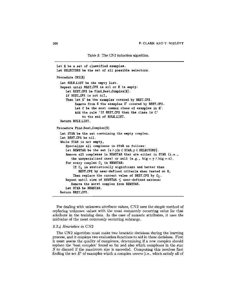
Table 3. The CN2 induction algorithm.
Let E be a set of classified examples.Let SELECTORS be the set of all possible selectors.
Procedure CN2(E)Let RULE-LIST be the empty list.Repeat until BEST.CPX is nil or E is empty:
Let BEST.CPX be Find-Best.Complex(E).If BEST.CPX is not nil,Then let E' be the examples covered by BEST.CPX.
Remove from E the examples E' covered by BEST.CPX.Let C be the most common class of examples in E'.Add the rule 'If BEST.CPX then the class is C'
to the end of RULE-LIST.Return RULE-LIST.
Procedure Find-Best.Complex(E)Let STAR be the set containing the empty complex.Let BEST.CPX be nil.While STAR is not empty,
Specialize all complexes in STAR as follows:Let NEWSTAR be the set {x A y|x 6 STAR, y € SELECTORS}.Remove all complexes in NEWSTAR that are either in STAR (i.e.,
the unspecialized ones) or null (e.g., big = y A big = n).For every complex Ci in NEWSTAR:
If Ci is statistically significant and better thanBEST.CPX by user-defined criteria when tested on E,
Then replace the current value of BEST.CPX by Ci.Repeat until size of NEWSTAR < user-defined maximum:
Remove the worst complex from NEWSTAR.Let STAR be NEWSTAR.
Return BEST.CPX.
For dealing with unknown attribute values, CN2 uses the simple method ofreplacing unknown values with the most commonly occurring value for thatattribute in the training data. In the case of numeric attributes, it uses themidvalue of the most commonly occurring subrange.
2.3.4 Heuristics in CN2The CN2 algorithm must make two heuristic decisions during the learning
process, and it employs two evaluation functions to aid in these decisions. Firstit must assess the quality of complexes, determining if a new complex shouldreplace the 'best complex' found so far and also which complexes in the star5 to discard if the maximum size is exceeded. Computing this involves firstfinding the set E' of examples which a complex covers (i.e., which satisfy all of
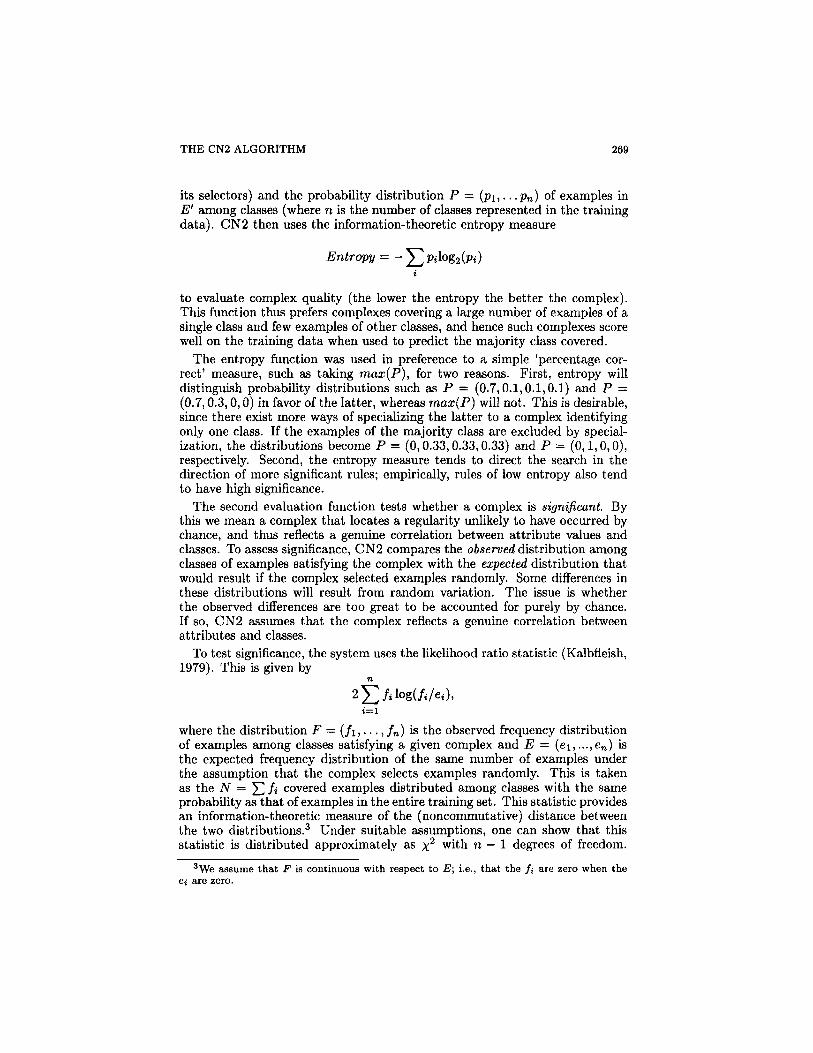
THE CN2 ALGORITHM 269
its selectors) and the probability distribution P = (p1,.. .pn) of examples inE' among classes (where n is the number of classes represented in the trainingdata). CN2 then uses the information-theoretic entropy measure
to evaluate complex quality (the lower the entropy the better the complex).This function thus prefers complexes covering a large number of examples of asingle class and few examples of other classes, and hence such complexes scorewell on the training data when used to predict the majority class covered.
The entropy function was used in preference to a simple 'percentage cor-rect' measure, such as taking max(P), for two reasons. First, entropy willdistinguish probability distributions such as P = (0.7,0.1,0.1,0.1) and P =(0.7,0.3,0,0) in favor of the latter, whereas max(P) will not. This is desirable,since there exist more ways of specializing the latter to a complex identifyingonly one class. If the examples of the majority class are excluded by special-ization, the distributions become P = (0,0.33,0.33,0.33) and P = (0,1,0,0),respectively. Second, the entropy measure tends to direct the search in thedirection of more significant rules; empirically, rules of low entropy also tendto have high significance.
The second evaluation function tests whether a complex is significant. Bythis we mean a complex that locates a regularity unlikely to have occurred bychance, and thus reflects a genuine correlation between attribute values andclasses. To assess significance, CN2 compares the observed distribution amongclasses of examples satisfying the complex with the expected distribution thatwould result if the complex selected examples randomly. Some differences inthese distributions will result from random variation. The issue is whetherthe observed differences are too great to be accounted for purely by chance.If so, CN2 assumes that the complex reflects a genuine correlation betweenattributes and classes.
To test significance, the system uses the likelihood ratio statistic (Kalbfleish,1979). This is given by
where the distribution F — (/1,..., fn) is the observed frequency distributionof examples among classes satisfying a given complex and E = (e1 , . . . ,en) isthe expected frequency distribution of the same number of examples underthe assumption that the complex selects examples randomly. This is takenas the N = ^3 ft covered examples distributed among classes with the sameprobability as that of examples in the entire training set. This statistic providesan information-theoretic measure of the (noncommutative) distance betweenthe two distributions.3 Under suitable assumptions, one can show that thisstatistic is distributed approximately as x2 with n — 1 degrees of freedom.
3We assume that F is continuous with respect to E; i.e., that the fi are zero when theei are zero.
270 P. CLARK AND T. NIBLETT
This provides a measure of indicates significance - the lower the score, themore likely that the apparent regularity is due to chance.
Thus these two functions - entropy and significance — serve to determinewhether complexes found during search are both 'good' (have high accuracywhen predicting the majority class covered) and 'reliable' (the high accuracy ontraining data is not just due to chance). CN2 uses these functions to repeatedlysearch for the 'best' complex that also passes some minimum threshold ofreliability until no more reliable complexes can be found.
2.4 A Bayesian classifierTo establish a reference point, we also implemented a simple Bayesian clas-
sifier and compared its behavior to that of the other algorithms.
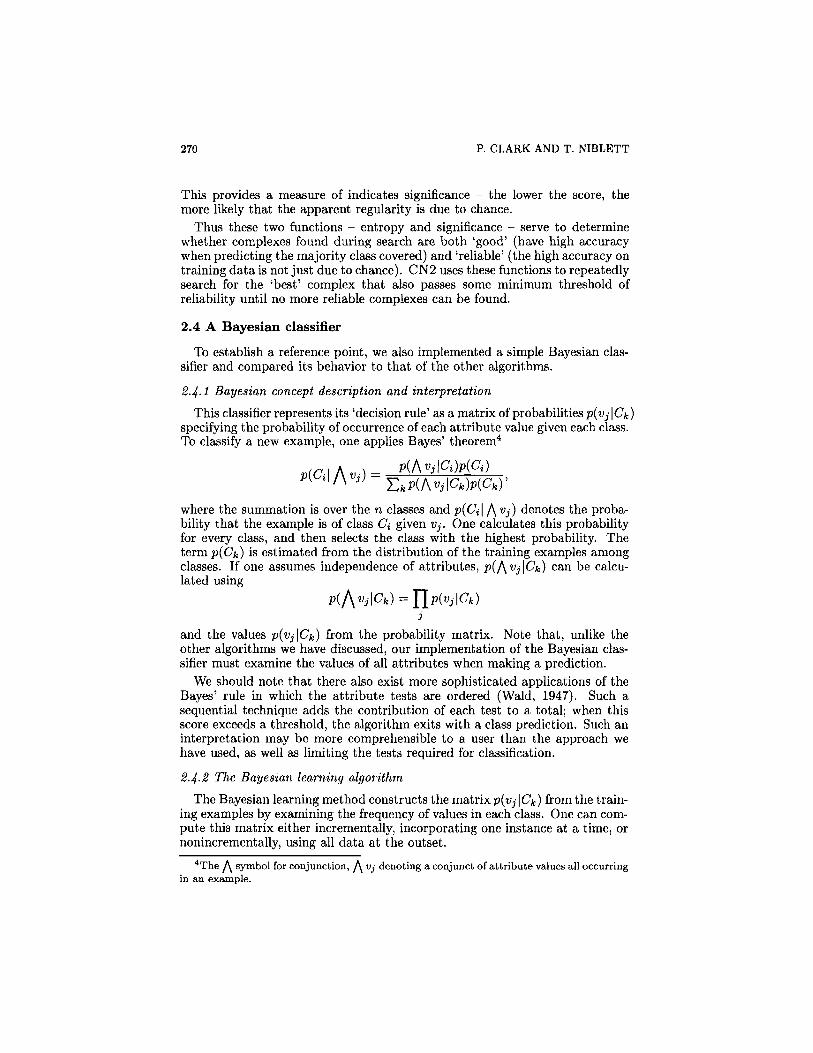
2.4.1 Bayesian concept description and interpretationThis classifier represents its 'decision rule' as a matrix of probabilities P(Vj \Ck)
specifying the probability of occurrence of each attribute value given each class.To classify a new example, one applies Bayes' theorem4
where the summation is over the n classes and p(Ci\ /\Vj) denotes the proba-bility that the example is of class (Ci given Vj. One calculates this probabilityfor every class, and then selects the class with the highest probability. Theterm p(Ck) is estimated from the distribution of the training examples amongclasses. If one assumes independence of attributes, p(f\Vj\Ck) can be calcu-lated using
and the values p(vj\Ck) from the probability matrix. Note that, unlike theother algorithms we have discussed, our implementation of the Bayesian clas-sifier must examine the values of all attributes when making a prediction.
We should note that there also exist more sophisticated applications of theBayes' rule in which the attribute tests are ordered (Wald, 1947). Such asequential technique adds the contribution of each test to a total; when thisscore exceeds a threshold, the algorithm exits with a class prediction. Such aninterpretation may be more comprehensible to a user than the approach wehave used, as well as limiting the tests required for classification.
2.4.2 The Bayesian learning algorithmThe Bayesian learning method constructs the matrix P(Vj \ Ck) from the train-
ing examples by examining the frequency of values in each class. One can com-pute this matrix either incrementally, incorporating one instance at a time, ornonincrementally, using all data at the outset.
4The /\ symbol for conjunction, ^ Vj denoting a conjunct of attribute values all occurringin an example.
THE CN2 ALGORITHM 271
2.4.3 Bayesian heuristicsSometimes a value of zero is calculated from the training data for some
elements of the p(vj\Ck) matrix. Like all elements of the matrix, this num-ber is subject to error due to the finite training data available. However, asclassification of new examples involves multiplying elements together, a zeroelement can have drastic effect, nullifying the effect of all other probabilities inthe multiplication. To avoid this, we assume that zero elements in the matrixwould, given more data, converge on a small, non-zero value and hence replacethe zeros with some appropriate estimate. In our implementation a value ofp(Ck] x (1/N) was used, where N is the number of training examples. Thefactor 1/N represents the increasing certainty that this element must have analmost-zero value with increasing size of training data.
2.5 The default rule
Finally, we examined a fifth 'algorithm' that simply assigns the most com-monly occurring class to all new examples, with no reference to their attributesat all. As we will see in Section 4, this simple procedure produced comparableperformance to that of the other algorithms in one of the domains, and thusprovided another useful reference point.
3. Time complexity of the algorithmsThe ASSISTANT, AQR and CN2 algorithms all search a very large space of
concept descriptions, and all use heuristics to guide this search. Furthermore,all three algorithms attempt to produce structures that are both consistentwith the training examples and as compact as possible. In the design of suchalgorithms, there is a tradeoff between execution speed and the size of theinduced structures. In each case, the exhaustive search for a smallest set ofstructures, although desirable, is computationally infeasible.
A major application of these algorithms is to extract useful information fromvery large databases, perhaps with millions of examples. With this in mind, itis worth examining the complexity of each algorithm. To be practical for verylarge problems, their behavior should be linear, or at least near-linear, in thenumber of examples and attributes.
Since the overall complexity of each algorithm is domain-dependent, we in-stead provide upper bounds for the critical components of the algorithms. Forexample, we do not consider the complexity of the cutoff procedure used byASSISTANT. In our treatment, we will use e to denote the size of the exampleset, a to stand for the number of attributes, and s to represent the maximumstar size (for CN2 and AQR). We also assume that each attribute is binaryvalued and that there are two classes.5
5One might also consider the complexity as a function of the number of distinct attributevalues and classes. We have not done this in our analysis.

272 P. CLARK AND T. NIBLETT
3.1 Time complexity of ASSISTANTThe critical component in ASSISTANT is the process of selecting a test at-
tribute on which to branch. Each such choice involves the following operations:1. For each attribute, example counts are put in an array, indexed by class
and attribute. This takes time O(e-a);2. The entropy function is calculated for each attribute, taking time O(a);3. Once the best attribute is found, the examples are divided into two sets;6
this takes time O(e).Therefore, the overall time for a single attribute choice is O(a.e). The timetaken to construct the complete tree depends very much on the structure of thetree. It seems reasonable to use the first figure only for comparative purposes,as argued above. Thus the amount of time taken by ASSISTANT for the basicattribute selection operation is a linear function of the number of examples,when the number of classes and attributes are held constant.
We should note that extensions to this algorithm that use real-valued at-tributes such as ACLS (Paterson & Niblett, 1982), must sort the examples byattribute value at the first stage. This increases the overall time bound toO(a . eloge).
3.2 Time complexity of CN2
The basic operation in CN2 is the specialization of the complexes in thecurrent star. The number of single-selector complexes without disjuncts is 2a.The number of intermediate complexes generated is at most a-s, and the timetaken to evaluate an example against a complex is bounded by O(a). Threesteps are required for this specialization operation:1. Multiplying each complex in the star by the set of single selector rules;
this takes time O(a .s ) ;2. Evaluation of each complex, taking time O(s.e.a);3. Sorting the complexes by value and then trimming the star, which takes
time O(a.s log(a.s)) .Therefore, the overall time for a single specialization step is bounded byO(a.s(e + log (a . s ) ) ) . As with ASSISTANT, the time required is a linear functionof the number of examples. If we restrict the size of the star to one, the timerequired has the same order as for ASSISTANT. In general, experience indicatesthat the time constants involved are somewhat less for ASSISTANT and othervariants on ID3 than for CN2.
3.3 Time complexity of AQRIn AQR, the basic operation is the specialization of complexes in a star.
This operation is similar to that of CN2, except that one only generates spe-
6With appropriate data structures, it may be possible to do much of this work in thefirst stage, but this does not affect the complexity class. Similarly, one can include anytermination test that is linear in the number of examples.
THE CN2 ALGORITHM 273
cializations that cause a negative example to be uncovered by complexes inAQR's star. We show the complexity of this operation is the same as that ofCN2. For each negative example, the following steps are performed:1. A negative example is found by iterating through the negative set. We
assume that the number of negative examples is not less than some fixedfraction of the entire example set. This takes time O(e.s);
2. The set of selectors that distinguish the negative example from the seedare found; this takes time O(a);
3. Each complex in the star is specialized by intersection with this set ofselectors, taking time O(a.s);
4. The resulting complexes are evaluated, which takes time O(a .s .e ) ;5. The complexes are sorted and the star trimmed, taking time O(a.s log(a.s)).
Thus, for each negative example the time is bounded by O(a.s(e + log(a.s))).This is the same figure as obtained for CN2. Observe that the number ofiterations of this process (making the star disjoint from a negative example) isbounded by the number of attributes, not by the number of examples.
In practice, although the order of time taken by the algorithms for this par-ticular operation of producing a new star is the same, CN2 is faster overallthan AQR. This is because the number of iterations of this operation is lowerin CN2 than in AQR, since CN2 may halt specialization of a complex beforeit performs perfectly on the training examples. Also, CN2 may halt the en-tire search for rules before all the training examples are covered if no furtherstatistically significant rules can be found.
3.4 Time complexity of the Bayesian classifier
The time complexity of the Bayes' classifier for generating a probabilitymatrix is O(a.e) , where a is the number of attributes and e the number ofexamples. This learning algorithm was substantially faster than the otheralgorithms because the run time is independent of the decision 'rule' generated.In addition, this basic operation is performed only once, unlike the abovealgorithms in which the basic operation is repeatedly applied.
3.5 Summary and actual run times
We have shown that the time complexity of the basic learning step for allthe algorithms tested is linear in the number of examples, with O(a • e) forASSISTANT and the Bayes' classifier and O(a • e • s) for AQR and CN2. Thisis an essential requirement for any algorithm that must work with very largedata sets.
However, the time complexity of the entire induction process, requiring iter-ation of the basic learning steps, is also important. With ideal noise-tolerantalgorithms, given a certain minimum number of examples, concept descrip-tions representing only the genuine regularities in the data should be induced.Additional examples should not cause the concept description to grow furtherand become overfitted, hence in this ideal case the above figures also represent
274 P. CLARK AND T. NIBLETT
the time complexity of the overall learning task. When this ideal is not met, aswhen one seeks a concept description that classifies the training data perfectly,the complexity increases. In such cases, CN2 would at worst induce e rulesof length a, giving an overall time complexity of O(a2 • e2 • s) (Chan, 1988).ASSISTANT sorts a total of e examples among a attributes for each level of thetree, giving an overall time complexity of O ( a 2 . e ) as the tree depth is boundedby a. The worst-case time complexity for AQR is similar to that for CN2.
The actual run times are revealing, although it is difficult to make quantita-tive comparisons due to differences in implementation language and method.Run times for each algorithm were obtained for the lymphography domain(Section 4.2.1) using a four-megabyte Sun 3/75. ASSISTANT, implemented inabout 5000 lines of Pascal, took one minute run time. CN2 and AQR, eachimplemented in about 400 lines of Prolog and with a value of fifteen for maxs-tar, took 15 and 170 minutes runtime respectively. The Bayesian classifier,implemented in 150 lines of Prolog, took a few seconds to calculate its prob-ability matrix. Although it is difficult to draw conclusions from the absoluterun times, it is our opinion that the ordering of these run times (Bayes fastest,followed by ASSISTANT, CN2 and AQR) is a fair reflection of the relativecomputation involved in using the algorithms. More detailed empirical com-parisons of time and memory requirements of ID3 and the AQ-based systemAQ11P have been conducted by O'Rorke (1982) and Jackson (1985) in thedomain of chess end games.
4. Experiments with the algorithmsOther aspects of the systems' behaviors lend themselves more to experimen-
tal study than analysis. Below we describe the dependent measures used inour experiments with the algorithms. After this, we describe the results of ourstudies with three natural domains and two artificial domains.
4.1 Dependent measuresIn addition to computational complexity, we are interested in two other
aspects of the algorithms' behaviors - classificational accuracy and syntacticcomplexity of the acquired structure. This twofold evaluation is motivated byconsidering these systems as knowledge-acquisition tools for expert systems.A useful system should induce rules that are accurate, so that they performwell, and comprehensible, so that they can be validated by an expert and usedfor explanation.
We measure each algorithm's classification accuracy by splitting the datainto a training set and a test set, presenting the algorithm with the training setto induce a concept description and then measuring the percentage of correctpredictions made by that concept description on the test set. Quinlan (1983,1987a) and others have taken a similar approach to measuring accuracy.
Cross-algorithm comparisons of the complexity of concept descriptions aredifficult due to the differences in representation and the degree of subjectivityinvolved in judging complexity. Thus, we will only compare the gross fea-tures of the knowledge structures induced by the different algorithms. For
THE CN2 ALGORITHM 275
ASSISTANT'S decision trees, we measure complexity by the number of nodes(including leaves) in the tree. For CN2 and AQR, we measure complexity bythe number of selectors in the final rule list and rule set respectively. Thesemeasures reveal the gross features of the induced decision rules. More detailedmeasures of rule complexity have been made by O'Rorke (1982) but are notused here. We assign a complexity of one to the default rule, based on itsequivalence to a decision tree with a single node.
Assessing the complexity of a Bayesian description is more difficult. Onecould count the number of elements in the p(Vj \Ck) matrix. Thus, for a domainwith n classes and a attributes, each with an average of v possible values, thecomplexity would be a x v x n. However, such a measure is independent ofthe training examples, and it ignores features of the matrix that may makeit more comprehensible (e.g., a few elements may be very large and the restsmall). Still, lacking any better measure, we provide the size of the matrix asa rough guide.
4.2 Experiments on natural domainsThe above algorithms were tested on three sets of medical data, which we
will describe shortly. These data were obtained from the Institute of Oncologyat the University Medical Center in Ljubljana, Yugoslavia (Kononenko et al.,1984). In each test, 70% of the training examples were selected at randomfrom the entire data set, and the remaining 30% of the data were used fortesting. The algorithms were all run on the same training data and theirinduced knowledge structures tested using the same test data. Five such testswere performed for each of the three domains, and the results were averaged.These data are thus identical to those used to test AQ15 in Michalski et al.(1986), though the particular random 70% and 30% samples are different. BothCN2 and AQR were given a value of 15 for maxstar in all runs.
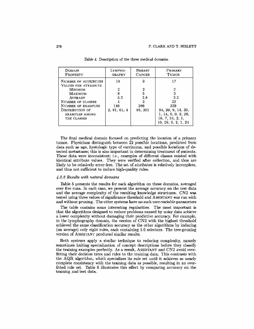
4.2.1 Three medical domainsTable 4 summarizes the characteristics of the three medical domains used
in the experiments. The first of these involved lymphography. For patientswith suspected cancer, it is important for physicians to distinguish betweenpatients that are healthy and those with metastases or malignant lymphoma.Patient data relating to this task were collected from Ljubljana's OncologyInstitute. These data were consistent; i.e., examples of any two classes werealways different. All the tested algorithms produced fairly simple and accuraterules. Unlike the other two domains, this data set was not submitted to adetailed checking after its original compilation by the Medical Center, andthus may contain errors in attribute values.
The second domain involved predicting whether patients who have under-gone breast cancer operations will experience recurrence of the illness withinfive years of the operation. The recurrence rate is about 30%, and hence suchprognosis is important for determining post-operational treatment. These datawere verified after collection, and thus are likely to be relatively free of errors.
276 P. CLARK AND T. NIBLETT
Table 4. Description of the three medical domains.
DOMAINPROPERTY
NUMBER OF ATTRIBUTES
LYMPHO-GRAPHY
18
BREASTCANCER
9
PRIMARYTUMOR
17VALUES PER ATTRIBUTE
MINIMUMMAXIMUMAVERAGE
NUMBER OF CLASSESNUMBER OF EXAMPLESDISTRIBUTION OF
EXAMPLES AMONGTHE CLASSES
283.34
1482, 81, 61, 4
252.82
28685, 201
232.2
22339
84, 20, 9, 14, 39,1, 14, 6, 0, 2, 28,16, 7, 24, 2, 1,10, 29, 6, 2, 1, 24
The final medical domain focused on predicting the location of a primarytumor. Physicians distinguish between 22 possible locations, predicted fromdata such as age, hystologic type of carcinoma, and possible locations of de-tected metastases; this is also important in determining treatment of patients.These data were inconsistent; i.e., examples of different classes existed withidentical attribute values. They were verified after collection, and thus arelikely to be relatively error-free. The set of attributes is relatively incomplete,and thus not sufficient to induce high-quality rules.
4-2.2 Results with natural domainsTable 5 presents the results for each algorithm on these domains, averaged
over five runs. In each case, we present the average accuracy on the test dataand the average complexity of the resulting knowledge structures. CN2 wastested using three values of significance threshold and ASSISTANT was run withand without pruning. The other systems have no such user-variable parameters
The table contains some interesting regularities. The most important isthat the algorithms designed to reduce problems caused by noisy data achievea lower complexity without damaging their predictive accuracy. For example,in the lymphography domain, the version of CN2 with the highest thresholdachieved the same classification accuracy as the other algorithms by inducing(on average) only eight rules, each containing 1.6 selectors. The tree-pruningversion of ASSISTANT produced similar results.
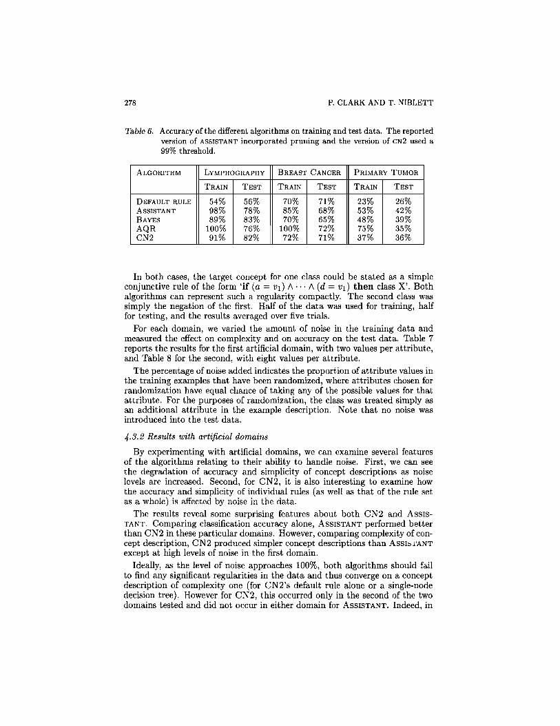
Both systems apply a similar technique to reducing complexity, namelysometimes halting specialization of concept descriptions before they classifythe training examples perfectly. As a result, ASSISTANT and CN2 avoid over-fitting their decision trees and rules to the training data. This contrasts withthe AQR algorithm, which specializes its rule set until it achieves as nearlycomplete consistency with the training data as possible, resulting in an over-fitted rule set. Table 6 illustrates this effect by comparing accuracy on thetraining and test data.

THE CN2 ALGORITHM 27'
T See discussion in Section 4.1 about difficulties in measuring the complexity ofBayesian classifiers.
The results also show that the Bayesian classifier does well, performing com-parably to the more sophisticated algorithms in all three domains and givingthe highest accuracy in the lymphography domain. Table 6 shows that thismethod regularly overfits the training data, but that its performance on thetest set is still good. Even more surprising is the behavior of the frequency-based default rule, which outperforms ASSISTANT and the Bayes' method onthe breast cancer domain. This suggests that there are virtually no significantcorrelations between attributes and classes in these data. This is reflected byCN2's inability to find significant rules in this domain at 99% threshold, sug-gesting that, in this domain at least, the significance test has been effective infiltering out rules representing chance regularities.
In general, the differences in performance seem to be due less to the learningalgorithms than to the nature of the domains; for example the best classifica-tion accuracy for lymphography was barely half as high as that for primarytumor. This suggests the need for additional studies to examine the role ofdomain regularity on learning.
4.3 Experiments on artificial domains
To better understand the effects of overfitting, we experimented with CN2and ASSISTANT on two artificial domains that let us control the amount ofnoise in the data.
4-S.I Two artificial domainsBoth domains contained twelve attributes and 200 examples that were evenly
distributed between two classes. They differed only in the number of valueseach attribute could take (two in the first domain and eight in the second).
Table 5. Accuracy and complexity of knowledge structures acquired by the algo-rithms in three natural domains. (Complexity for the Bayes' classifier isthe size of the probability matrix.)
ALGORITHM
DEFAULT RULEASSISTANT
NO PRUNINGPRUNING
BAYESAQRCN2
90% THRESH.95% THRESH.99% THRESH.
LYMPHOGRAPHYACCUR.
56%
79%78%83%76%
78%81%82%
COMP.
14136
240t76
242212
BREAST CANCERACCUR.
71%
62%68%65%72%
70%70%71%
COMP.1
11244
54ot208
28204
PRIMARY TUMORACCUR.
26%
40%42%39%35%
37%36%36%
COMP.1
17852
465^562
334219
278 P. CLARK AND T. NIBLETT
Table 6. Accuracy of the different algorithms on training and test data. The reportedversion of ASSISTANT incorporated pruning and the version of CN2 used a99% threshold.
ALGORITHM
DEFAULT RULEASSISTANTBAYESAQRCN2
LYMPHOGRAPHYTRAIN
54%98%89%
100%91%
TEST
56%78%83%76%82%
BREAST CANCERTRAIN
70%85%70%
100%72%
TEST71%68%65%72%71%
PRIMARY TUMORTRAIN23%53%48%75%37%
TEST
26%42%39%35%36%
In both cases, the target concept for one class could be stated as a simpleconjunctive rule of the form 'if (a = v1) A • • • A (d = v1) then class X'. Bothalgorithms can represent such a regularity compactly. The second class wassimply the negation of the first. Half of the data was used for training, halffor testing, and the results averaged over five trials.
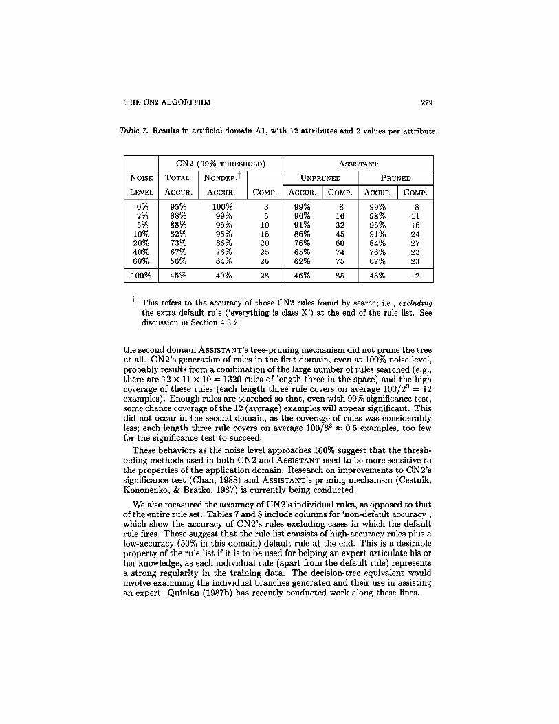
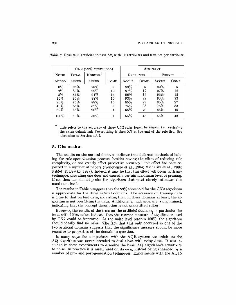
For each domain, we varied the amount of noise in the training data andmeasured the effect on complexity and on accuracy on the test data. Table 7reports the results for the first artificial domain, with two values per attribute,and Table 8 for the second, with eight values per attribute.
The percentage of noise added indicates the proportion of attribute values inthe training examples that have been randomized, where attributes chosen forrandomization have equal chance of taking any of the possible values for thatattribute. For the purposes of randomization, the class was treated simply asan additional attribute in the example description. Note that no noise wasintroduced into the test data.
4.3.2 Results with artificial domainsBy experimenting with artificial domains, we can examine several features
of the algorithms relating to their ability to handle noise. First, we can seethe degradation of accuracy and simplicity of concept descriptions as noiselevels are increased. Second, for CN2, it is also interesting to examine howthe accuracy and simplicity of individual rules (as well as that of the rule setas a whole) is affected by noise in the data.
The results reveal some surprising features about both CN2 and ASSIS-TANT. Comparing classification accuracy alone, ASSISTANT performed betterthan CN2 in these particular domains. However, comparing complexity of con-cept description, CN2 produced simpler concept descriptions than ASSISTANTexcept at high levels of noise in the first domain.
Ideally, as the level of noise approaches 100%, both algorithms should failto find any significant regularities in the data and thus converge on a conceptdescription of complexity one (for CN2's default rule alone or a single-nodedecision tree). However for CN2, this occurred only in the second of the twodomains tested and did not occur in either domain for ASSISTANT. Indeed, in
THE CN2 ALGORITHM 279
Table 7. Results in artificial domain Al, with 12 attributes and 2 values per attribute
NOISELEVEL
0%2%5%
10%20%40%60%
100%
CN2 (99% THRESHOLD)TOTALACCUR.
95%88%88%82%73%67%56%45%
NONDEF.T
ACCUR.100%99%95%95%86%76%64%49%
COMP.
35
101520252628
ASSISTANTUNPRUNED
ACCUR.99%96%91%86%76%65%62%46%
COMP.8
16324560747585
PRUNEDACCUR.
99%98%95%91%84%76%67%43%
COMP.8
11162427232312
T This refers to the accuracy of those CN2 rules found by search; i.e., excludingthe extra default rule ('everything is class X') at the end of the rule list. Seediscussion in Section 4.3.2.
the second domain ASSISTANT'S tree-pruning mechanism did not prune the treeat all. CN2's generation of rules in the first domain, even at 100% noise level,probably results from a combination of the large number of rules searched (e.g.,there are 12x11x10 = 1320 rules of length three in the space) and the highcoverage of these rules (each length three rule covers on average 100/23 — 12examples). Enough rules are searched so that, even with 99% significance test,some chance coverage of the 12 (average) examples will appear significant. Thisdid not occur in the second domain, as the coverage of rules was considerablyless; each length three rule covers on average 100/83 s 0.5 examples, too fewfor the significance test to succeed.
These behaviors as the noise level approaches 100% suggest that the thresh-olding methods used in both CN2 and ASSISTANT need to be more sensitive tothe properties of the application domain. Research on improvements to CN2'ssignificance test (Chan, 1988) and ASSISTANT'S pruning mechanism (Cestnik,Kononenko, & Bratko, 1987) is currently being conducted.
We also measured the accuracy of CN2's individual rules, as opposed to thatof the entire rule set. Tables 7 and 8 include columns for 'non-default accuracy',which show the accuracy of CN2's rules excluding cases in which the defaultrule fires. These suggest that the rule list consists of high-accuracy rules plus alow-accuracy (50% in this domain) default rule at the end. This is a desirableproperty of the rule list if it is to be used for helping an expert articulate his orher knowledge, as each individual rule (apart from the default rule) representsa strong regularity in the training data. The decision-tree equivalent wouldinvolve examining the individual branches generated and their use in assistingan expert. Quinlan (1987b) has recently conducted work along these lines.
280 P. CLARK AND T. NIBLETT
Table 8. Results in artificial domain A2, with 12 attributes and 8 values per attribute
NOISEADDED
0%2%5%
10%20%40%60%
100%
CN2 (99% THRESHOLD)TOTALACCUR.
93%83%86%80%73%68%63%50%
NONDEF.T
ACCUR.98%99%94%98%88%82%90%58%
COMP.
810131015541
ASSISTANTUNPRUNED
ACCUR.99%97%96%93%85%75%66%55%
COMP.6
12152227334043
PRUNEDACCUR.
99%97%96%93%85%75%66%55%
COMP.6
12152227334043
* This refers to the accuracy of those CN2 rules found by search; i.e., excludingthe extra default rule ('everything is class X') at the end of the rule list. Seediscussion in Section 4.3.2.
5. DiscussionThe results on the natural domains indicate that different methods of halt-
ing the rule specialization process, besides having the effect of reducing rulecomplexity, do not greatly affect predictive accuracy. This effect has been re-ported in a number of papers (Kononenko et al., 1984; Michalski et al., 1986;Niblett & Bratko, 1987). Indeed, it may be that this effect will occur with anytechnique, providing one does not exceed a certain maximum level of pruning.If so, then one should prefer the algorithm that most closely estimates thismaximum level.
The results in Table 6 suggest that the 99% threshold for the CN2 algorithmis appropriate for the three natural domains. The accuracy on training datais close to that on test data, indicating that, in these domains at least, the al-gorithm is not overfitting the data. Additionally, high accuracy is maintained,indicating that the concept description is not underfitted either.
However, the results of the tests on the artificial domains, in particular thetests with 100% noise, indicate that the current measure of significance usedby CN2 could be improved. As the noise level reaches 100%, the algorithmshould ideally find no rules. The fact that this only occurred in one of thetwo artificial domains suggests that the significance measure should be moresensitive to properties of the domain in question.
In many ways the comparisons with the AQR system are unfair, as theAQ algorithm was never intended to deal alone with noisy data. It was in-cluded in these experiments to examine the basic AQ algorithm's sensitivityto noise. In practice it is rarely used on its own, instead being enhanced by anumber of pre- and post-generation techniques. Experiments with the AQ15
THE CN2 ALGORITHM 281
system (Michalski et al., 1986) show that with post-pruning of the rules anda probability-based or 'flexible matching' method for rule application, one canachieve results similar to those of CN2 and ASSISTANT in terms of accuracyand complexity.
The principal advantage of CN2 over AQR is that the former algorithmsupports a cutoff mechanism - it does not restrict its search to only thoserules that are consistent with the training data. CN2 demonstrates that onecan successfully control the search through the larger space of inconsistent ruleswith the use of judiciously chosen search heuristics. Second, by including amechanism for handling noise in the algorithm itself, we have achieved a simplemethod for generating noise tolerant if-then rules that is easy to reproduce andanalyze. In addition, interactive approaches to induction, in which the userinteracts with the system during and after rule generation, introduce additionalrequirements, such as the need for good explanation facilities. In such cases,the logical rule interpretation used by CN2 should have practical advantagesover the more complex probabilistic rule interpretation needed to apply order-independent rules (such as those generated by AQR) in which conflicts mayoccur.
Another result of interest is the high performance of the Bayesian classifier.Although the independence assumption of the classifier may be unjustified inthe domains tested, it did not perform significantly worse in terms of accu-racy than other algorithms, and it remains an open question as to how sen-sitive Bayesian methods are to violated independence assumptions. Althoughthe probability matrices produced by the tested classifier are difficult to com-prehend, the experiments suggest that variants of the Bayes' classifier whichproduce more comprehensible decision procedures would be worthy of furtherinvestigation.
6. ConclusionsIn this paper we have demonstrated CN2, an induction algorithm that com-
bines the best features of the ID3 and AQ algorithms, allowing the applicationof statistical methods similar to tree pruning in the generation of if-then rules.The CN2 system is similar to ASSISTANT in its efficiency and ability to handlenoisy data, whereas it partially shares the representation language and flexiblesearch strategy of AQR. By incorporating a mechanism for handling noise intothe algorithm itself, a method for inducing if-then rules has been achieved thatis noise-tolerant, simple to analyze, and easy to reproduce.
The experiments we have conducted show that, in noisy domains, the CN2algorithm has comparable performance to that of ASSISTANT. By inducingconcept descriptions based on if-then rules, CN2 provides a tool for assistingin the construction of knowledge-based systems where one desires classifica-tion procedures based on rules rather than decision trees. The most obviousimprovement to the algorithm, suggested by the results on artificial domains,is an improvement to the significance measure used.
282 P. CLARK AND T. NIBLETT
AcknowledgementsWe thank Donald Michie and Claude Sammut for their careful reading and
valuable comments on earlier drafts of this paper. We also thank Pat Lang-ley and the reviewers for their detailed comments and suggestions about thepresentation. We are grateful to G. Klanjscek, M. Soklic, and M. Zwitterof the University Medical Center, Ljubljana for the use of the medical dataand to I. Kononenko for its conversion to a form suitable for the inductionalgorithms. This work was supported by the Office of Naval Research undercontract N00014-85-G-0243 as part of the Cognitive Science Research Program.
ReferencesCestnik, B., Kononenko, I., & Bratko, I. (1987). ASSISTANT 86: A knowledge-
elicitation tool for sophisticated users. Proceedings of the Second EuropeanWorking Session on Learning (pp. 31-45). Bled, Yugoslavia: Sigma Press.
Chan, P. K. (1988). A critical review of CN2: A polythetic classifier sys-tem (Technical Report CS-88-09). Nashville, TN: Vanderbilt University,Department of Computer Science.
Iba, W., Wogulis, J., & Langley, P. (1988). Trading off simplicity and coveragein incremental concept learning. Proceedings of the Fifth InternationalConference on Machine Learning (pp. 73-79). Ann Arbor, MI: MorganKaufmann.
Jackson, J. (1985). Economics of automatic generation of rules from examplesin a chess end-game (Technical Report UIUCDCS-F 85-932). Urbana:University of Illinois, Computer Science Department.
Kalbfleish, J. (1979). Probability and statistical inference (Vol. 2). New York:Springer-Verlag.
Kononenko, I., Bratko, I., & Roskar, E. (1984). Experiments in automaticlearning of medical diagnostic rules (Technical Report). Ljubljana, Yu-goslavia: E. Kardelj University, Faculty of Electrical Engineering.
Michalski, R. S. (1969). On the quasi-minimal solution of the general coveringproblem. Proceedings of the Fifth International Symposium on Informa-tion Processing (pp. 125-128). Bled, Yugoslavia.
Michalski, R. S., & Chilausky, R. (1980). Learning by being told and learn-ing from examples: An experimental comparison of the two methods ofknowledge acquisition in the context of developing an expert system forsoybean disease diagnosis. International Journal of Policy Analysis andInformation Systems, 4 , 125-160.
Michalski, R. S., & Larson, J. (1983). Incremental generation of VL1 hypothe-ses: The underlying methodology and the description of the program AQl 1(Technical Report ISG 83-5). Urbana: University of Illinois, ComputerScience Department.
Michalski, R. S., Mozetic, I., Hong, J., & Lavrac, N. (1986). The multi-purpose incremental learning system AQl5 and its testing application tothree medical domains. Proceedings of the Fifth National Conference onArtificial Intelligence (pp. 1041-1045). Philadelphia: Morgan Kaufmann.

THE CN2 ALGORITHM 283
Mowforth, P. (1986). Some applications with inductive expert system shells(TIOP 86-002). Glasgow, Scotland: Turing Institute.
Niblett, T. (1987). Constructing decision trees in noisy domains. Proceedingsof the Second European Working Session on Learning (pp. 67-78). Bled,Yugoslavia: Sigma Press.
Niblett, T., & Bratko, I. (1987). Learning decision rules in noisy domains. InM. A. Bramer (Ed.), Research and development in expert systems (Vol. 3).Cambridge: Cambridge University Press.
O'Rorke, P. (1982). A comparative study of inductive learning systems AQ11Pand ID3 using a chess end-game test problem (Technical Report ISG 82-2). Urbana: University of Illinois, Computer Science Department.
Paterson, A., & Niblett, T. (1982). ACLS manual, Version 1 (Technical Re-port). Glasgow, Scotland: Intelligent Terminals Limited.
Quinlan, J. R. (1983). Learning efficient classification procedures and their ap-plication to chess end games. In R. S. Michalski, J. G. Carbonell, & T. M.Mitchell (Eds.), Machine learning: An artificial intelligence approach. LosAltos, CA: Morgan Kaufmann.
Quinlan, J. R. (1987a). Simplifying decision trees. International Journal ofMan-Machine Studies, 27, 221-234.
Quinlan, J. R. (1987b). Generating production rules from decision trees. Pro-ceedings of the Tenth International Joint Conference on Artificial Intelli-gence (pp. 304-307). Milan, Italy: Morgan Kaufmann.
Quinlan, J. R., Compton, P. J., Horn, K. A., & Lazarus, L. (1987). Induc-tive knowledge acquisition: A case study. Applications of expert systems.Wokingham, England: Addison-Wesley.
Rivest, R. L. (1987). Learning decision lists. Machine Learning, 2, 229-246.Wald, A. (1947). Sequential analysis. New York: Wiley.